SECURITIZATION AND OPTIMAL RETENTION UNDER …chairegestiondesrisques.hec.ca/wp-content/uploads/2015/07/Malekan... · Securitization Introduction ... 101 . viii . List of abreviations

HEC MONTRÉAL École affiliée à l’Université de Montréal

SECURITIZATION AND OPTIMAL RETENTION UNDER MORAL HAZARD

Par

Sara Malekan

Thèse présentée en vue de l’obtention du grade de Ph. D. en administration

(option Finance)

Avril 2015

© Sara Malekan, 2015

HEC MONTRÉAL École affiliée à l’Université de Montréal

Cette thèse intitulée :

SECURITIZATION AND OPTIMAL RETENTION UNDER MORAL HAZARD

Présentée par :

Sara Malekan

a été évaluée par un jury composé des personnes suivantes :

Pascal François HEC Montréal

Président-rapporteur

Georges Dionne HEC Montréal

Directeur de recherche

Michèle Breton HEC Montréal

Membre du jury

Marie-Claude Beaulieu Université Laval

Examinateur externe

Fabien Chauny HEC Montréal

Représentant du directeur de HEC Montréal

RÉSUMÉ

La titrisation est l'une des innovations les plus importantes sur les marchés financiers. C’est le

processus de mise en commun des actifs financiers (prêts), de les arranger, de les convertir en

actifs financiers structurés et de les vendre sous forme de tranches correspondant à des

investisseurs ayant des appétits différents pour le risque. La structure des tranches correspond à

des risques de défaut différents et à des rendements différents. Elle ressemble à une structure de

capital donnant un ordre de priorité dans l’allocation des défauts.

En dépit de tous les avantages de la titrisation, elle est souvent soupçonnée d'être l'une des causes

principales de la récente crise financière en raison du problème d'aléa moral qui réduit la

motivation des banques dans le dépistage des prêteurs et dans la surveillance des prêts. Cette forme

de risque moral est maximale lorsque les banques transfèrent tous leurs prêts aux marchés

financiers. La rétention d’une quantité de prêts par la banque semble être une sage solution pour

diminuer le problème d'aléa moral associé à la titrisation. Elle est fréquemment utilisée pour

revitaliser les marchés de titrisation depuis la crise financière.

Méthodes de recherche : Notre objectif est de trouver la forme de rétention optimale pour les

prêts sous l'aléa moral. Nous analyserons la titrisation optimale sous l'aléa moral en appliquant la

méthodologie de la détermination endogène des contrats pour ces produits afin d'obtenir le partage

optimal du risque entre les vendeurs et les acheteurs de ces produits.

Mots-clés: titrisation , rétention optimale , aléa moral , modèle principal-agent , tranching ,

rehaussement de crédit , le risque systémique.

ABSTRACT

Securitization is one of the most important innovations in financial markets. It is the process of

pooling financial assets, packaging and converting them into securities and then selling them in

the form of prioritized capital structure of claims to dispersed investors.

In spite of all the advantages of securitization, it is often suspected to be one of the main causes of

the recent financial crisis due to the moral hazard problem in lender screening and monitoring.

Tranche retention seems to be an optimal solution to solve the moral hazard problem of

securitization and is used frequently to revitalise securitization markets.

Research method: Our objective is to find the optimal amount and form of retention for

securitized products under moral hazard. We analyze the incentive contracting of securitized

products under moral hazard and apply the security design methodology to these products in order

to obtain the optimal risk sharing between sellers and buyers of these products.

Keywords: Securitization, optimal retention, moral hazard, principal-agent model, tranching,

credit enhancement, systemic risk.

v

Table of Contents

RÉSUMÉ ................................................................................................................................................. iv

ABSTRACT .............................................................................................................................................. v

List of figures ......................................................................................................................................... viii

List of abreviations .................................................................................................................................. ix

Dedication ................................................................................................................................................. x

Acknowledgment ..................................................................................................................................... xi

Chapter 1:Literature Review of Securitization in the Banking Industry ..................................................... 1

Securitization Introduction ........................................................................................................................ 2

1.1 "Originate-to-distribute" revolution .................................................................................................... 2

1.2 Problems of securitization ................................................................................................................... 6

1. 2. 1 Adverse selection ..................................................................................................................... 11

1. 2. 2 Moral Hazard ........................................................................................................................... 14

1.3 Solutions ........................................................................................................................................... 18

1. 3. 1 Solutions for adverse selection ................................................................................................ 21

1. 3. 2 Solutions to moral hazard ........................................................................................................ 25

1.4 Design of research on moral hazard .................................................................................................. 31

1. 4. 1 Best contract for principal-agent model ................................................................................... 32

Chapter 2:One Tranche Without Credit Enhancement Procedure ............................................................ 36

Introduction ............................................................................................................................................. 37

2.1 Motivation ......................................................................................................................................... 39

2.2 Contributions..................................................................................................................................... 39

2.3 The model ......................................................................................................................................... 42

2.3.1 Investors’ objective function ...................................................................................................... 44

2.3.2 Participation constraint .............................................................................................................. 45

2.3.3 Incentive compatibility constraint .............................................................................................. 47

vi

2.3.4 Technology constraint ................................................................................................................ 48

2.3.5 Analyzing the result ................................................................................................................... 52

2.4 Conclusion ........................................................................................................................................ 54

Chapter 3:Structured Asset-backed Securitization without Systemic Risk ............................................... 56

Introduction ............................................................................................................................................. 57

3.1 Extension of the model ..................................................................................................................... 59






3.2 Conditional distribution of loss ......................................................................................................... 73


3.3 Conclusion ........................................................................................................................................ 82

Chapter 4:Structured Asset-backed Securitization with Systemic Risk .................................................... 85

Introduction ............................................................................................................................................. 86

4.1 Derivation of the model .................................................................................................................... 87






4.2 Conclusion ...................................................................................................................................... 102

Appendix ................................................................................................................................................... 104

References ................................................................................................................................................. 114

vii

List of figures

Figure 1: Simplified Overview of the Securitization Process…………………………………...…38

Figure 2: Optimal Securitization Contract under Ex Ante Moral Hazard…………………..….…54

Figure 3: Optimal Securitization Contract under credit enhancement procedure…………..……72

Figure 4: Optimal Securitization Contract with conditional distribution of loss and credit enhancement……………………………………………………...……………………………...…...…82

Figure 5: Optimal Securitization Contract with credit enhancement and systemic risk……..…101

viii

List of abreviations

Originate-to-distribute OTD

Credit risk transfer CRT

Special purpose vehicle SPV

Loan-to-value LTV

European Union EU

Collateralized loan obligation CLO

Monotone likelihood ratio property MLRP

ix

Dedication

This thesis is dedicated to my father, who inspired me to pursue doctoral studies,

to my mother and sister, who helped me with my baby,

to my daughter, Sophia, for her patience, and

to my husband who was always there for me.

x

Acknowledgment

First and foremost, I am grateful to my PhD supervisor Prof. Georges Dionne for his valuable

advice and guidance throughout the duration of my studies. His support and ideas were

instrumental in improving the quality of the work.

I would like to thank the administrative staff at HEC, including Ms. Lise Cloutier, Ms. Claire

Boisvert, and Ms. Julie Bilodeau, and Ms. Nathalie Bilodeau.

I am also thankful to all my friends, namely, Ms. Kiana Basiri, Mr. Xiaozhou Zhou, and Mr. Cédric

Okou, who made my time at HEC more enjoyable and more memorable.

xi

Chapter 1:

Literature Review of Securitization in the Banking Industry

Securitization Introduction

Securitization is one of the most important innovations in financial markets. It is a process of

converting illiquid loans that cannot be sold readily to third-party investors into liquid securities

and selling them to dispersed investors.

Because of the attractiveness of securitization for financial market participants, its application has

widely been extended in recent years. In April 2011, the volume of outstanding securitized assets

reached $11 trillion, which is substantially greater than the overall outstanding marketable US

Treasury securities of $8 trillion (US Department of the Treasury, 2011).

In spite of all its advantages and widespread application, securitization is often suspected of being

one of the main reasons for the recent financial crisis. That is why in the following pages we survey

the literature on the revolutions that securitization brings to the market. We focus on major

problems of securitization which are related to the recent financial crisis as well as previously

proposed solutions in order to make our contribution to the literature more clear.

1.1 "Originate-to-distribute" revolution

The dramatic increase in the application of securitization during the last few decades has changed

the traditional role of financial intermediaries from "originating and holding" to "originating and

selling." This transfer to the "originate-to-distribute" model has significant implications for all

market participants, including the originating banks, the borrowing firms, the individuals, the

investors, and the regulators.

2

“Originate-to-distribute” (OTD) model can be “socially desirable” according to the advantages

that it may create. This financial innovation enhances the accessibility of credits and standardizes

origination of the loans. Overall it improves the efficiency of credit market performance by

creating more complete markets and facilitating the liquidity transformation that was the

fundamental role traditionally performed by financial intermediaries (Diamond and Dybvig

(1983)).

As a result, “Originating and selling” has increased liquidity in capital markets and provided the

originating banks with additional sources of financing by allowing originators to remove the issued

loans from their balance sheet and use the proceeds for other purposes or even to originate new

loans (Coval, Jurek and Stafford (2009)).

Accordingly it is no more required for the banks to hold as many illiquid assets on balance sheet

and since they can offer new loans by selling old loans they are not supposed to just relying on

issuing new liabilities. These additional sources of financing increase the capacity of the banks'

loan supply which depends upon business cycle conditions and banks' risk position. These features

possibly lead to an increase in lending and promoting economic growth. Pavel and Phillis (1987)

mention all the above features as issuers’ incentives for securitization. They find that issuers want

to have high risk or leverage as well as to mitigate or diversify risks. All these developments

together help banks to extend credit reaction to the cost of funds of external shocks (Coval, Jurek

and Stafford (2009); Loutskina (2011)).

For example, by using a large sample of European banks, Altunbas, Gambacorta and Marques-

Ibanez (2009) demonstrate that the application of securitization could protect the bank's loan

supply from the consequences of monetary policy shocks. With securitization banks are less

3

dependent on deposits (traditional funding sources) and protected against interest-rate shocks,

whether or not these shocks are derived by monetary policy (Altunbas, Gambacorta and Marques-

Ibanez (2009); Gambacorta and Marques‐Ibanez (2011); Goswami, Jobst and Long (2009)).

This evolution of "originate-to-distribute" model has some positive consequences in borrowers’

relationship by increasing the access to financial markets for all the participants even those who

had no access to the market before. It also alleviates borrower's financial constraints and provides

additional financing (Gande and Saunders (2012 )) as well as increasing access to debt capital for

borrowers (Drucker and Puri (2009)).

As a result borrowers have access to a wide range of loans with better terms and conditions,

because, in the presence of securitization, the risk of borrowing spreads among a dispersed group

of investors that can bear more risk than individual banks. It reduces borrower's cost of capital as

a result of valuable risk-sharing benefits from sale of loans to other investors in the secondary loan

market (Gupta, Singh and Zebedee (2008); Parlour and Winton (2013)).

For the above reasons securitization is considered as one of the most efficient approaches to

dispense credit risk since it improves risk sharing and decreases the cost of capital for lenders by

dropping off the regulated capital. Issuers can also lower their cost of capital by securitizing low

risk assets which protects them against bankruptcy (Ambrose, LaCour-Little and Sanders (2003);

Ayotte and Gaon (2005); Gorton and Souleles (2007); Greenbaum and Thakor (1987); Minton,

Sanders and Strahan (2004)).

4

Improving risk sharing and reducing the bank's cost of capital are extensively mentioned as

benefits of securitization in the literature. In contrast Cheng, Dhaliwal and Neamtiu (2011) indicate

that asset securitization increases cost of capital as a result of higher information uncertainty which

can be seen in higher bid-ask spreads and dispersion. It is because of emergence of credit derivative

markets with loan securitization activity that have transformed credit risk management by banks.

Overall "Originate-to-distribute" model provides this opportunity for the banks to diversify their

asset portfolio, reach parts of the credit spectrum and transfer credit risk from their balance sheets

to other economic agents. Securitization allows an originating bank to earn their fees and then

transfer the interest rate and credit risks to outside investors. A potential advantage is that the

banking system can reduce its exposure to risk that threatens its stability by transferring it to those

most able to bear it (Brunnermeier (2008); Pennacchi (1988)). Therefore banks benefit the healthy

spread due to securitization. Another advantage is that investors’ desire to access a high yield on

rated investments is satisfied.

Credit risk transfer (CRT), however, can have a blurred outcome on the fragility of the financial

system (Allen and Carletti (2006)). On one hand it is helpful specially if the financial system is

fragile and the credit risk is transferred to the non-bank sectors; it allows banks to better diversify

their risks which improve financial stability (Wagner and Marsh (2006)). On the other hand, higher

portfolio diversification caused by credit risk transfer can reduce financial stability and in this

manner confirms the ambiguous implications for total welfare (Wagner (2005)).

Credit risk transfer can lead to contagion across different sectors in the financial system and

thereby to a reduction in total welfare (Kiff and Kisser (2010)). It can also lead to an unprecedented

credit expansion that helped feed recent financial crisis (Brunnermeier (2008)).

5

Wagner (2007) shows that although credit risk transfer improves asset liquidity for banks it also

encourages them to take on higher risks which then offset the positive impact of higher liquidity.

So far some advantages and disadvantages of securitization have been discussed. These have also

been considered in numerous other articles (Dell’Ariccia, Igan and Laeven (2012); Demyanyk and

Van Hemert (2011); Gorton (2009); Gorton and Metrick (2012); Kashyap and Stein (2000); Keys,

Mukherjee, Seru and Vig (2008); Keys, Mukherjee, Seru and Vig (2009); Kothari, Loutskina and

Nikolaev (2006); Loutskina (2006); Loutskina and Strahan (2009); Mian and Sufi (2008);

Morrison (2005); Parlour and Plantin (2008); Rajan, Seru and Vig (2010)).

The disadvantages of securitization are the result of some problems which are discussed next.

1.2 Problems of securitization

The above evidences, taken together, suggest that the secondary loan market has significantly

transformed the nature of the banking activities and the borrower and lender relationship.

Traditionally, banks held the issuing loans until they are repaid; they produced information on the

nature of borrowers (screening) and monitored the borrowers of originated loans. The emergence

of an active secondary market for bank loans in which loans are pooled, tranched, and then resolved

through securitization, possibly diluted screening and monitoring activities carried out by banks

(Diamond (1984); Holmstrom and Tirole (1997)) even if it allows for additional loans to be made.

In this way, although banks uphold a central role in originating loan and evaluating credit risk,

they lose their importance as primary holders of illiquid loans (Altunbas, Gambacorta and

Marques-Ibanez (2009); Gupta, Singh and Zebedee (2008)).

6

This transformation has some negative consequences like increasing complexity and reducing

transparency in loan origination that leads to breakdown of lending relationships. Furthermore, the

securitization process reduces the market participants’ incentive to learn about underlying

collateral information (Park (2013)).

Reduction in monitoring, in addition to breakdown of lending relationship, leads to suboptimal

investment decision and harsher covenants (Drucker and Puri (2009)), as well as creating

difficulties in debt renegotiation (Carey, Prowse, Rea and Udell (1994)). The participating

investors who buy the loans without having a lending relationship with the borrowers are then

expected to be at an information disadvantage when buying a loan originated by a bank. Selling

the loans in the secondary market (securitization) could result in moral hazard and adverse

selection problems (Gorton and Pennacchi (1995); Pennacchi (1988)). Because of securitization

only low quality loans are securitized (adverse selection) and loans that can be sold are not initially

screened, or not subsequently monitored (moral hazard).

Keys et al. (2008), Demyanyk & Van Hemert (2011) and Dell’Ariccia et al. (2012) investigate the

reduction in lending standards due to securitization. Gorton (2010) goes one step further by

considering structure of MBS in order to find out why this reduction happens. Parlour & Plantin

(2008) established a theoretical model to show evidence of some of the above outlined effects.

Nevertheless, from an empirical standpoint, it is not obvious which of these effects dominate.

The emergence of secondary loan market deteriorated the role of the monetary policy.

Securitization provides banks with an additional funding sources and may weaken the impact of

central banks on the lending channel by reducing the efficiency of the traditional interest-rate

policy (Kuttner (2000)). Estrella (2002) suggests that central banks should rely on mechanisms

7

beyond the interest rate, in order to increase the impact of monetary policy. Stein (2011) explains

how monetary policy can affect bank lending and real activity to achieve financial stability.

Another problem within the secondary loan market that is related to securitization process is poor

credit quality of structured products. One reason for this problem is attractiveness of structured

products for rating agencies due to higher collected fees that they bring out for rating agencies

which leads to superior ratings for structured products compared to other bonds and securities

(Brunnermeier (2008)). These credit rating agencies’ incentives to issue higher rating was also

considered as a possible cause of recent financial crisis.

Another reason for poor quality of structured products is that rating agencies were not diligent in

assessing credit risk associated with off-balance sheet securitization activities. Barth, Ormazabal

and Taylor (2011) examines the association source of credit risk with asset securitization and find

that securitizing firms’ credit risk is not only associated with retained portion of the securitized

assets but is also associated with the non-retained portion of the securitized assets which is not

considered in assessment of rating agencies. On the other hand rating agencies perceive that firms’

credit risk exposure is only associated with the contractual retained interest in the securitized assets

and not associated with the non-retained portion of the securitized assets. Rating agencies’

assessment of the firm’s credit risk is based on private information about asset securitization that

can be presented by credit ratings. Credit ratings can be affected by factors other than the credit

risk of the bank, such as rating agency incentives for issuing particular ratings. Credit risk can also

be measured by bond spreads which is based on publicly available information about asset

securitization. Bond spread measurement might be incomplete, but is not likely affected by

incentives for assessing a particular level of risk. As a result credit risk assessments by bond market

can be more reliable than those by rating agencies. Bond market assesses that the firm’s credit risk

8

is associated with both the retained and non-retained portions of securitized assets which indicate

the deficiency of rating agencies in assessing credit risk.

Higher ratings by rating agencies provide firms with opportunity to obtain additional financing at

lower cost which can be used to fund further asset securitization (Morgenson and Story (2010);

Rosenkranz (2009); Sorkin (2009)). On the other hand these higher credit rating, give the banks a

wrong sense of confidence that they are far away from any trouble and encourage them to take on

tail risks through issuing more short term claims rather than long term claims. This tendency

increases the possibility that banks become illiquid and incapable of rolling over financing

(Diamond and Rajan (2009)).

The above situation can become worse by increasing the incentives of levered institutions to

become more illiquid with the expectation that future interest rates would be low (Diamond and

Rajan (2009 )). Now it becomes obvious why banks were willing to take illiquidity risk in case of

a sharp downturn, especially when there was a great possibility of increasing the liquidity and

cutting the interest rates by Federal Reserve (the so-called “Greenspan Put”).

In general the nature of modern banking is unstable and risky. Shleifer and Vishny (2010) present

a model in the context of securitization and leverage and show that a levered bank is naturally

volatile. Gennaioli, Shleifer and Vishny (2012) show that even without leverage, financial

intermediaries can be volatile and fragile, because investors neglect certain unlikely risks.

In summary, the securitized products are affected by deficiencies in the following aspects:

Complexity, Transparency, Contracting, Rating,

9

Pricing, and Regulation

These could lead to major problems, such as adverse selection and moral hazard.

10

1. 2. 1 Adverse selection

The complexity due to the securitization process, which bundles the loans, tranches them into

different risk categories and then sells diverse packages of loans is that it decreases the

transparency of loans' quality to participating investors. This reduction in transparency together

with bank's superior information about the borrowers' quality give rise to information asymmetry

between lenders and investors which leads to an adverse selection problem.

Adverse selection problem results in decreasing the quality of the loans in the securitized pool.

Elul (2011) applies a regression approach to identify the relationship between securitization and

loan performance and he found that securitized mortgages perform worse than portfolio loans. He

attributes this result to adverse selection of poorer loans into securitized pools.

Downing, Jaffee and Wallace (2009) offer a sharp-test to evaluate the adverse selection problem

in the context of federally guaranteed mortgages. Their findings provide strong empirical support

to verify that the quality of securitized assets is lower (“lemons”) compared to assets that are not

sold through special purpose vehicles (SPVs).

There is vast uncertainty over how these securities should be valued which leads to considerable

fear of information asymmetries about the quality of the underlying assets and banks’ exposures

to these securities. The issue of adverse selection raises the question for participating investors if

they can trust the banks, in the sense that banks are not selling lemons. Are banks selling loans of

borrowers about whom they have negative private information that is unobservable by outside

investors or are they selling off the loans due to appropriate motives such as capital relief, risk

diversification, improving balance-sheet liquidity, and reducing financing frictions and their cost

of capital?

11

Akerlof (1970) shows that, in the context of incomplete markets, informational asymmetries may

lead to "lemon problem" that cause the breakdown of used-car market. Hart and Holmstrom (2008)

and Hellwig (2009) pay attention to the same "lemon problem," in the secondary loan market after

the onset of financial crisis. They demonstrate that during financial crisis, there were a lot of

concerns about the quality of the loans due to rise in information asymmetry about the quality of

trading assets. Market participants performed as they expected to do in the perfect market.

Investors pulled out their money and demanded a huge discount on any unknown quality assets.

Uninformed investors did not fear that the sellers were trying to get rid of low quality assets while

keeping the good ones. As a result liquidity in the market decreased and the price declined as the

quantity sold increased (Firla-Cuchra and Jenkinson (2005)).

Decline in the pricing system aggravated the difficulties in the financial market (see Hellwig 2009).

One of the main reasons behind this turndown in the asset valuation of banks was not only the loss

on the underlying assets of securities, but also the general reaction of the market participants to

the lemon problem. As a result of this awareness about the lemon problem and the involving risk

spread among all market participants, all such assets lost their value and this process extended

from a small sector of the market through the rest. Great part of banks' holding assets suddenly

lost much of their value. The pricing system undermined as expectations changed (Colander,

Goldberg, Haas, Juselius, Kirman, Lux and Sloth (2009)).

Colander, Goldberg, Haas, Juselius, Kirman, Lux and Sloth (2009) and Gorton and Souleles (2007)

reinvestigate the pricing of asset backed securities and informational role of financial prices and

financial markets in the presence of the lemon problem. They show that before securitization, asset

trading could transmit information, while in the presence of securitization this information

transmission seems to have broken down. They interpret this as securitization has to somewhat

12

bring about a loss of information by anonymous intermediation (often multiple) between

borrowers and lenders. In his way, the buyer of structured financial products would not have spent

any time and effort to gather information regarding his far away counterparts, and the

informational gathering has been outsourced to rating agencies. This centralized information

processing by rating agencies, rather than the dispersed one in traditional credit relationships,

initiated a severe loss of information. As a result, standard loan default model have fallen short

considerably in recent years (Rajan, Seru and Vig (2010)).

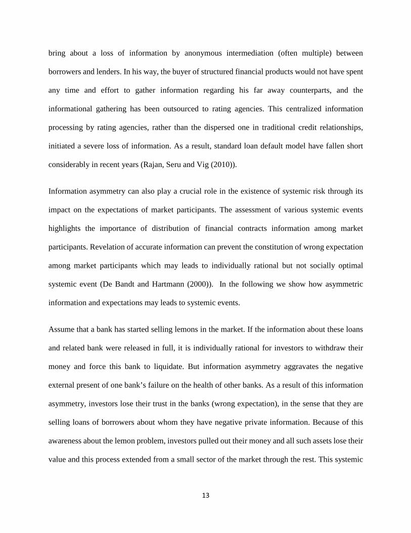
Information asymmetry can also play a crucial role in the existence of systemic risk through its

impact on the expectations of market participants. The assessment of various systemic events

highlights the importance of distribution of financial contracts information among market

participants. Revelation of accurate information can prevent the constitution of wrong expectation

among market participants which may leads to individually rational but not socially optimal

systemic event (De Bandt and Hartmann (2000)). In the following we show how asymmetric

information and expectations may leads to systemic events.

Assume that a bank has started selling lemons in the market. If the information about these loans

and related bank were released in full, it is individually rational for investors to withdraw their

money and force this bank to liquidate. But information asymmetry aggravates the negative

external present of one bank’s failure on the health of other banks. As a result of this information

asymmetry, investors lose their trust in the banks (wrong expectation), in the sense that they are

selling loans of borrowers about whom they have negative private information. Because of this

awareness about the lemon problem, investors pulled out their money and all such assets lose their

value and this process extended from a small sector of the market through the rest. This systemic

13

event might still have been individually rational but it is not socially optimal because it leads to

capital losses due to decline in asset valuation below the normal market level.

The lemon problem can also lead to a volatile financial market because the levered banks which

are depending significantly on investors’ sentiment have to liquidate a fraction of this assets on

balance sheet in order to keep a haircut level (the margin between the actual market value of a

security and the value assessed by investors’ sentiment) even though the actual quality of these

assets is high (Shleifer and Vishny (2010)). The lemon problem decreases the market value of

collateral securities which makes the investor to evaluate these securities as being worth less than

they actually are to give itself a cushion.

Alternatively originate-to-distribute model of credit may persuade banks to originate bad loans to

increase their fee income and then sell them off in the active secondary market which may lead to

underperformance of borrowers in long run along with valuation loss of their total assets in

comparison with their peers (Berndt and Gupta (2009)). Additional detailed discussions of adverse

selection problem can be found in (Ashcraft and Schuermann (2008); Gorton (2009); Rajan, Seru

and Vig (2010)).

1. 2. 2 Moral Hazard

Due to the increase of securitization, credit quality and lending standard have declined. This is

because other financial institutions, rather than the banks, bear the major part of the securitized

risk. Banks basically face only the pipeline risk of holding a loan for some months until the risks

are passed on to investors (Angelides and Thomas (2011)). If banks are not exposed to the default

risk of the originated loans they would not have enough incentive to be vigilant in approving loan

applications and monitoring loans in order to control and uphold the loans' quality. Taking off the

14

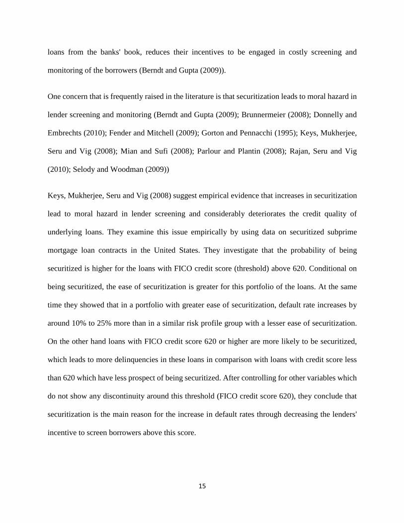
loans from the banks' book, reduces their incentives to be engaged in costly screening and

monitoring of the borrowers (Berndt and Gupta (2009)).

One concern that is frequently raised in the literature is that securitization leads to moral hazard in

lender screening and monitoring (Berndt and Gupta (2009); Brunnermeier (2008); Donnelly and

Embrechts (2010); Fender and Mitchell (2009); Gorton and Pennacchi (1995); Keys, Mukherjee,

Seru and Vig (2008); Mian and Sufi (2008); Parlour and Plantin (2008); Rajan, Seru and Vig

(2010); Selody and Woodman (2009))

Keys, Mukherjee, Seru and Vig (2008) suggest empirical evidence that increases in securitization

lead to moral hazard in lender screening and considerably deteriorates the credit quality of

underlying loans. They examine this issue empirically by using data on securitized subprime

mortgage loan contracts in the United States. They investigate that the probability of being

securitized is higher for the loans with FICO credit score (threshold) above 620. Conditional on

being securitized, the ease of securitization is greater for this portfolio of the loans. At the same

time they showed that in a portfolio with greater ease of securitization, default rate increases by

around 10% to 25% more than in a similar risk profile group with a lesser ease of securitization.

On the other hand loans with FICO credit score 620 or higher are more likely to be securitized,

which leads to more delinquencies in these loans in comparison with loans with credit score less

than 620 which have less prospect of being securitized. After controlling for other variables which

do not show any discontinuity around this threshold (FICO credit score 620), they conclude that

securitization is the main reason for the increase in default rates through decreasing the lenders'

incentive to screen borrowers above this score.

15

After accepting the term of the loan contract by borrowers and signing it between the lender and

borrower, the loan can be sold as part of the securitized pool to investors. When investors buy

these loans as part of a securitized pool, they only notice the "hard information" about the

borrowers (e.g. FICO score) and the contractual terms such as loan-to-value (LTV) ratio and

interest rates (Keys, Mukherjee, Seru and Vig (2008)). "Hard information" is defined as

information that is easy to measure, transmit and contract upon. To rate tranches of the securitized

pool, rating agencies use the same information about the borrowers and loan terms as investors use

to buy the loans. Since securitization increases the distance between the originators and investors,

and "soft information" (e.g., a measure of future income stability, provided years of documentation

and joint income status) about the borrowers is unavailable to third party, lenders choose not to

collect "soft information" about the borrowers. "Soft information", by definition, is something that

is not easy to contract upon and transmit, while the lender has to exert an unobservable effort to

collect soft information (Stein (2002)).

Accordingly, even though there is compensation for lenders to gather "hard information" about the

borrowers, their incentives to collect "soft information" depend on the extent to which they are

supposed to bear the risk of originated loans (Gorton and Pennacchi (1995); Parlour and Plantin

(2008); Rajan, Seru and Vig (2010)).

Keys, Mukherjee, Seru and Vig (2008) proposed that the only way that may persuade lenders to

incur the cost of obtaining "soft information" is that the signal provided by the borrowers' "hard

information" is not as much necessary while there is enough chance that lenders would retain the

loan on its balance sheet.

16

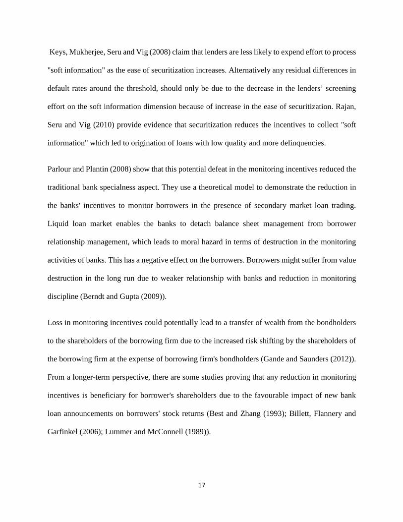
Keys, Mukherjee, Seru and Vig (2008) claim that lenders are less likely to expend effort to process

"soft information" as the ease of securitization increases. Alternatively any residual differences in

default rates around the threshold, should only be due to the decrease in the lenders’ screening

effort on the soft information dimension because of increase in the ease of securitization. Rajan,

Seru and Vig (2010) provide evidence that securitization reduces the incentives to collect "soft

information" which led to origination of loans with low quality and more delinquencies.

Parlour and Plantin (2008) show that this potential defeat in the monitoring incentives reduced the

traditional bank specialness aspect. They use a theoretical model to demonstrate the reduction in

the banks' incentives to monitor borrowers in the presence of secondary market loan trading.

Liquid loan market enables the banks to detach balance sheet management from borrower

relationship management, which leads to moral hazard in terms of destruction in the monitoring

activities of banks. This has a negative effect on the borrowers. Borrowers might suffer from value

destruction in the long run due to weaker relationship with banks and reduction in monitoring

discipline (Berndt and Gupta (2009)).

Loss in monitoring incentives could potentially lead to a transfer of wealth from the bondholders

to the shareholders of the borrowing firm due to the increased risk shifting by the shareholders of

the borrowing firm at the expense of borrowing firm's bondholders (Gande and Saunders (2012)).

From a longer-term perspective, there are some studies proving that any reduction in monitoring

incentives is beneficiary for borrower's shareholders due to the favourable impact of new bank

loan announcements on borrowers' stock returns (Best and Zhang (1993); Billett, Flannery and

Garfinkel (2006); Lummer and McConnell (1989)).

17

On the contrary, Billett, Flannery and Garfinkel (2006) show that the bank loans announcement

resulted in the negative abnormal returns in the long-run for the borrowing firm. From a short-term

perspective, most studies have shown positive abnormal returns for borrower's shareholders in

contrast to the announcement of other forms of corporate financing such as common stock,

preferred stock, straight debt and convertible debt (Berndt and Gupta (2009)). In general the

literature, on the effects of loan sales on the borrower’s stock price is rather controversial. While

Dahiya, Puri and Saunders (2003) recognized a negative effect of lending bank announcement of

the sale of a borrower’s loans, Gande and Saunders (2012) documented the reverse (positive)

announcement effect.

1.3 Solutions

At present, several policy questions arise from the above discussions for regulatory authorities.

The first question is that, in spite of all these benefits and weaknesses mentioned earlier, does the

shift to originate-to-distribute model create value in the financial system or not? Is it socially

desirable? If so, should these authorities put any restriction on these activities of the banks in order

to skip the costs and take more advantage from them that leads to additional value creation? Should

the regulatory authorities put into effect the enhancement of disclosure of the information about

banks’ activities in the loan sales market? What will be the long run effect of these regulations on

the borrowing firms and individuals, the banking system and, overall, the market?

18

Empirical evidence alone is not sufficient to answer all of these questions, as there are both positive

and negative effects of originate-to-distribute model. Ultimately, these issues must also be

considered theoretically which the focus of our research is.

In spite of all the advantages that securitization brings out to the economy and the financial system,

the financial crisis that began in August 2007 drew attention to this fact that advantageous financial

innovation such as securitization can become a source of financial instability if industry practice

and regulation do not keep pace with innovation (Selody and Woodman (2009)).

It is becoming important for regulators and market participants to understand the costs and benefits

of securitization so that they can appropriately improve the incentives and scope of securitization

to mitigate this information cost. Berndt and Gupta (2009) believe that the highly deregulated

nature of the secondary loan market is perhaps one of the main reasons for the occurrence of the

moral hazard and adverse selection problems. Stein (2011) explains the consequence of

unregulated private money creation on establishment of unstable market which make it necessary

to put in force supplementary policy together with open-market operation.

In summary we can mention the general solution for previously mentioned deficiencies:

Complexity: reducing the complexity of securitized products

Transparency: enhancing the availability and quality of information, making

securitization transparent and based on standards

Contracting: improve contractual part of securitization by carefully setting out the criteria

for loan eligibility for a pool

19

Ratings: improving the reliability and use of ratings by imposing new regulations on the

rating agencies, given the great responsibility generally attributed to their perceived failures

to mitigate rating agencies conflicts of interest.

Pricing: improve market functioning, take into consideration the risk premia and liquidity

premia for the pricing of structured products and impose new regulation to oblige banks to

have sufficient funds to satisfy their solvency.

Regulation: propose specific rules addressing both traditional financial institution and other

components of the “shadow banking system” focusing on the reforms to how securitization

should be done

Reviving securitization markets and bringing back investors’ confidence call for a coordinating

effort on all industry participants, investors, and regulators. There must be explicit or implicit

contractual design features to mitigate these obvious problems. Improving the design of securitized

products can result in significant reductions in the uncertainty surrounding credit quality and a

reduced need for monitoring (Selody and Woodman (2009)).

With the intention of achieving the above goal, it is necessary to change the structure of securitized

products in the way that they become less complex and opaque while at the same time they ensure

the alignment of incentives among various participants in the intermediation chain (Fender and

Mitchell (2009a); Paligorova (2009))

20

1. 3. 1 Solutions for adverse selection

The adverse selection issue has been studied extensively in the corporate finance and insurance

literatures. Different solutions can be extended for securitization to convince investors that there

are no incentive problems and reduce the agency problem. For example, DeMarzo and Duffie

(1999) develop a “hidden knowledge” model, in which the issuer earns the knowledge after signing

the contract. In this models, retaining a larger fraction of the issue is viewed as a signal of high

project value for privately informed issuer (DeMarzo and Duffie (1999); Leland and Pyle (1977)).

Implicit contract features such as the part of the loan retention or implicit guarantees against default

may make loan sales possible and in that way reduce the adverse selection problem (Gorton and

Pennacchi (1995)).

Recently some important models of securitization with the focus on asymmetric information issue

were proposed. Glaeser and Kallal (1997) and Riddiough (1997) address the adverse selection

problem in which an informed issuer optimally designs risky asset-backed securities with

asymmetric information and liquidation motives and then sells them in the market. This requires

the creation of low-risk and low information-sensitivity securities.

Dang, Gorton and Holmstrom (2009) support this idea that the issuance of information-insensitive

securities can resolve adverse selection problem. They approve that the attractiveness of security

design come from the fact that it reduces the incentives to privately acquire information. In this

case the value of these securities is independent of the information known only by the informed

issuer. Information-insensitive securities are liquid and can be traded easily in the financial market.

Park (2013) empirically demonstrates that in reality the main reason of applying securitization is

to generate information-insensitive securities. In this case the credit risk of the underlying

21

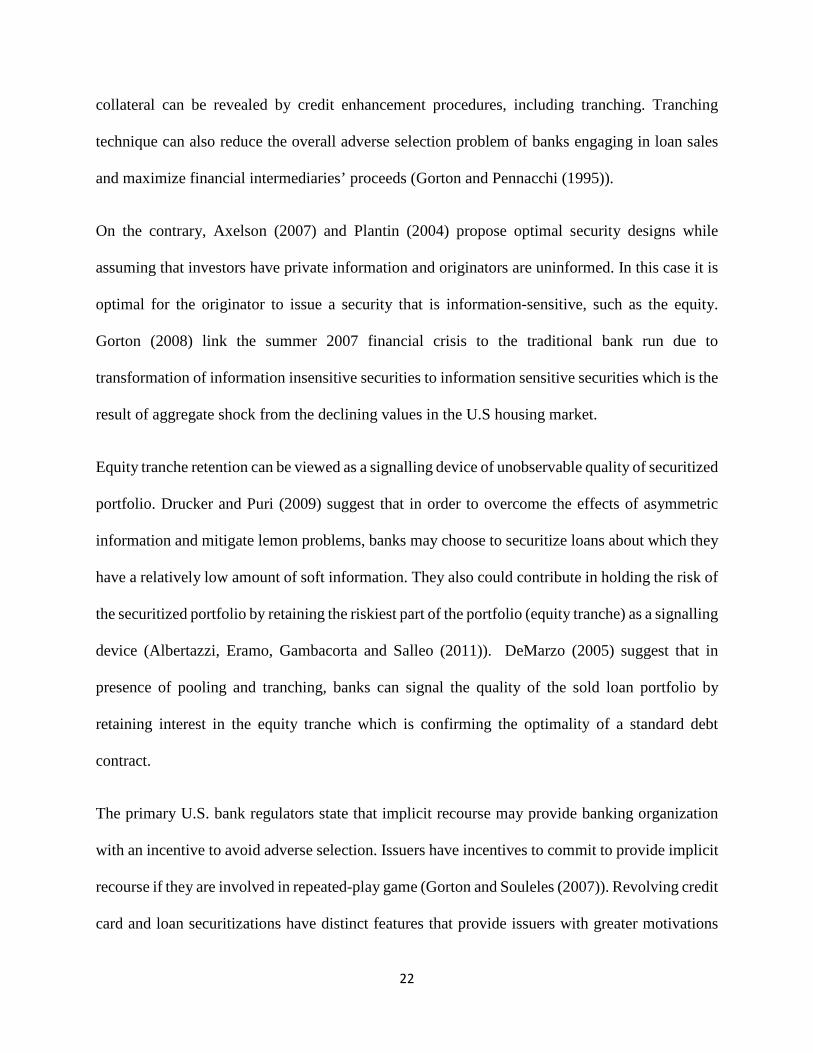
collateral can be revealed by credit enhancement procedures, including tranching. Tranching

technique can also reduce the overall adverse selection problem of banks engaging in loan sales

and maximize financial intermediaries’ proceeds (Gorton and Pennacchi (1995)).

On the contrary, Axelson (2007) and Plantin (2004) propose optimal security designs while

assuming that investors have private information and originators are uninformed. In this case it is

optimal for the originator to issue a security that is information-sensitive, such as the equity.

Gorton (2008) link the summer 2007 financial crisis to the traditional bank run due to

transformation of information insensitive securities to information sensitive securities which is the

result of aggregate shock from the declining values in the U.S housing market.

Equity tranche retention can be viewed as a signalling device of unobservable quality of securitized

portfolio. Drucker and Puri (2009) suggest that in order to overcome the effects of asymmetric

information and mitigate lemon problems, banks may choose to securitize loans about which they

have a relatively low amount of soft information. They also could contribute in holding the risk of

the securitized portfolio by retaining the riskiest part of the portfolio (equity tranche) as a signalling

device (Albertazzi, Eramo, Gambacorta and Salleo (2011)). DeMarzo (2005) suggest that in

presence of pooling and tranching, banks can signal the quality of the sold loan portfolio by

retaining interest in the equity tranche which is confirming the optimality of a standard debt

contract.

The primary U.S. bank regulators state that implicit recourse may provide banking organization

with an incentive to avoid adverse selection. Issuers have incentives to commit to provide implicit

recourse if they are involved in repeated-play game (Gorton and Souleles (2007)). Revolving credit

card and loan securitizations have distinct features that provide issuers with greater motivations

22

and ability to provide implicit recourse than in other securitizations (Calomiris and Mason (2004);

Higgins and Mason (2004)). Chen, Liu and Ryan (2008) believe that implicit recourse is unlikely

to have any significant effect on mortgages and commercial loans securitizations.

Reputational concerns could prevent banks from selling lemons, because they deal with investors

on a continuing basis and securitization process is not a once in a lifetime process (Fender and

Mitchell (2009a)). On the other hand if the present value of the future profits from securitization

would be above the cost of on balance sheet financing, reputational concerns can provide incentive

for the banks to mitigate adverse selection problem by determining the likelihood of loan default

and select which loan to put into the SPV (Gorton and Souleles (2007)). Banks might even choose

to securitize loans of better-than-average (although unobservable) quality, when trying to improve

their reputation (Albertazzi, Eramo, Gambacorta and Salleo (2011)). Gande, Puri, Saunders and

Walter (1997) and Kroszner and Rajan (1994) emphasize the same dynamics for banks who

underwrite the securities that are issued by their borrowing firms.

Albertazzi, Eramo, Gambacorta and Salleo (2011) investigate adverse selection problem of

securitization from the empirical contract theory view point and its alleviation by analyzing the

rich dataset on securitization in Italy. Overall, they suggest the following solutions to alleviate the

adverse selection problem: selling less opaque loans, using signalling devices (i.e. retaining a share

of the equity tranche) and building up a reputation for not undermining the lending standards.

Pooling of assets have an information-destruction effect that may augment adverse selection

problem, but at the same time it can play a role in overcoming this problem faced by uninformed

investors (Firla-Cuchra and Jenkinson (2005)). DeMarzo and Duffie (1999) and DeMarzo (2005)

develop models to demonstrate the trade-offs between adverse selection issue of pooling assets

23

(because it eliminates the advantage of asset-specific private information “information destruction

effect”) against “risk-diversification effect” of pooling (because it creates a potentially large low-

risk pool, and associated securities, that are less sensitive to the seller’s private information) for

informed issuer. They prove how tranching can be optimal together with pooling in presence of

asymmetric information, for large enough pools of assets. The intuition is as follow: as the size of

asset pool increases, the information destruction effect which leads to illiquidity can be outweigh

with the risk diversification effect of pooling.

Axelson (2007), Boot and Thakor (1993), Plantin (2004) and Riddiough (1997) also add some

explanations to the value creation effect of pooling and tranching under asymmetric information

by proposing theoretical models in the presence of various investors with different level of private

information. The basic intuition of their models is that there is a separating equilibrium by creating

an essentially riskless senior tranche which attracts unsophisticated investors who have low ability

to screen the underlying assets. Investors with more private information are attracted to more junior

tranches which allow the banks to re-cycle their capital and to raise the return to their private

information ratio.

On the other hand, the optimal security design allows banks to restructure the lemon pools into

tranched securities and overcome the adverse selection problem between informed investors who

buy the riskier junior tranches and uninformed investors who buy the senior tranches. As

Riddiough (1997) suggest even if asymmetric information steer the creation of a senior tranche,

several junior tranches might be formed to serve particular tastes of different investors with the

aim to facilitate the placement of the information-sensitive tranches in the market.

24

Agency conflicts can also play an important role in amplifying the adverse selection problem.

Drucker and Mayer (2008) point at the exploitation of inside information by underwriters due to

their advantage in secondary loan markets. In association with this finding, Drucker and Puri

(2009), Gorton and Pennacchi (1995) and Sufi (2007) look into the ways to mitigate these agency

conflicts through appropriate contract terms and conditions.

Regulatory supervision in the secondary loan market together with additional disclosure

requirement on all market participants with the aim of better transparency could, to some extent,

reduce agency conflicts and as a result resolve the adverse selection problem (Berndt and Gupta

(2009)).

1. 3. 2 Solutions to moral hazard

Regulatory oversight alone cannot resolve moral hazard problem which is the result of information

asymmetries in the OTD market on the lenders side. Keys, Mukherjee, Seru and Vig (2009) support

this idea by examining the consequences of existing regulations on the quality of mortgage loans

originations in the OTD market with the purpose of mitigating moral hazard problems. They find

that the quality of loan origination varies inversely with the amount of regulation; more regulated

lenders originate loans of worse quality. On the other hand the overall default rates for less

regulated banks were lower than high regulated banks.

As an alternative stronger risk management departments with greater bargaining power inside the

bank may have the power to resolve the moral hazard problem. By measuring the share of risk

manager's compensation from the total compensation which is given to the five highest-paid

executives in the institution, Keys, Mukherjee, Seru and Vig (2009) show that brokers with a

powerful risk management department have lower default rates on the originated mortgages. Ellul

25

and Yerramilli (2013) also provide some evidence that financial institution with a weak risk

management department are more prone to take excessive risk that brought about the financial

crisis.

Having more lenders inside a mortgage pool which is associated to more competition leads to

having a portfolio of loans with higher quality. Higher diversity reduces default rates and provides

this opportunity for the issuer of the pools to benchmark the quality of the loans against each other.

Keys, Mukherjee, Seru and Vig (2009) indicate that more competition among lenders result in

better performance evaluation and consequently to some extent can mitigate the moral hazard

problem. This relative performance evaluation could somewhat mitigate the moral hazard problem

(Gibbons and Murphy (1991)).

Reputational concerns play an important role in mitigating moral hazard problem. Keys,

Mukherjee, Seru and Vig (2009) provide some evidence that recommended banks with higher

reputation tend to be more conservative and try to keep their quality by, for example, keeping more

deposits, or more liquid assets which results in origination of more carefully screened and higher

quality loans in the OTD market. Overall, their evidence suggests that using market forces as an

internal device to align lenders’ incentives with that of the investors (like the one discussed in our

research), is more efficient in mitigating moral hazard in the OTD market than external policies

that impose stricter lender regulations which fail to align lenders’ incentives.

One possible solution for moral hazard problem, as an internal device to align lenders’ incentives,

is to impose restriction on the originated banks by requiring them to keep at least a certain

percentage of those loans on their books or to have skin in the game. This can be interpreted as the

fragility of lightly regulated originators’ capital structure and support the Dodd-Frank Law

26

approach intended to mitigate moral hazard by requiring a minimum level of risk retention by

originators.

Selody and Woodman (2009) propose that retaining a portion of an issue of a new debt with

intention of sharing the default risk of loans can result in the improvement of incentives alignment.

This may prevent banks from originating bad loans and give them more incentive to monitor

borrowers (Berndt and Gupta (2009)).

If participation of banks in risk sharing is sufficient, they would have enough motivation to perform

appropriate due diligence on loan origination, continuously monitor the behaviour of borrowers,

and, perhaps, represent warranties on the quality of loans and the underwriting process (Selody

and Woodman (2009)).

Donnelly and Embrechts (2010) go one step further by proposing that the banks should hold onto

the riskiest part of the loan pool in order to be exposed to the risk of loan defaults and have enough

incentives to control and preserve the quality of the originated loans. In practice, this did not always

take place, and as a result misalignment of incentives may have played a role in reducing the

lending standards and distorting the quality of loans originated in the OTD market (Brunnermeier

(2008); Dell’Ariccia, Igan and Laeven (2012); Keys, Mukherjee, Seru and Vig (2008); Mian and

Sufi (2008); Rajan (2006)).

Overall, tranche retention is considered as one of the most effective ways to align incentives

between originators and investors. There exist different retention mechanisms with considerably

different impact on the originators' efforts and incentives in screening and monitoring the

borrowers. Three general types of tranche retention are as follows:

27

Equity tranche retention

Mezzanine tranche retention

Vertical slice retention

Vertical slice retention is referred to retaining a percentage share of each of the tranches. Different

retention mechanisms have different impact on the screening level, due to different sensitivities to

a systematic risk factor which plays an important role in the determination of borrowers, default

probabilities and asset values (Fender and Mitchell (2009a); Fender and Mitchell (2009b)).

Showing different sensitivities implies that the effectiveness of tranche retention in aligning

incentives will be a function of tranche thickness, the return of assets, the size of the retained

interest, the economy’s position in the cycle (the state of the macro economy) and most importantly

how it is configured.

Vertical slice retention might be suboptimal in aligning incentives to monitor borrowers. Equity

tranche is more sensitive to the realisation of systemic risk than the entire portfolio. Because the

equity tranche will be exhausted when there is a large probability of a systemic risk it could

decrease the originator’s incentive to make a screening effort. In this case it would be better to

hold also mezzanine tranche (Fender and Mitchell (2009b)). Their focus is on associating different

screening effort across different retention mechanism rather than deriving an optimal profit

maximization contract for the originator.

Chen, Liu and Ryan (2008) investigate the determinants of the size of the equity tranche retention

by estimating the association between banks’ equity risk and the characteristics of the securitized

loans. They find that banks must retain larger equity tranche when the pool is riskier or the credit

risk is less externally verifiable to outside investors. In other words the structure of retention is not

28

independent of the risks of the pool (underlying portfolio). Their result is consistent with Dionne

and Harchaoui (2008), Haensel and Krahnen (2007) and Niu and Richardson (2006) who

investigate the relation between the measures of firms’ equity risk to their off-balance sheet

positions arising from securitizations. These papers conclude that the amount of equity risk which

is endured by firms is associated with both the retained and non-retained portions of the securitized

assets. Chen, Liu and Ryan (2008) show that the amount of equity risk associated with asset

securitization varies with the type of asset securitized. Moody’s Investor Service (2002) also

investigates the link of ultimate amount of risk transfer to specific structure of the transaction.

These findings are related to the literature on the equity risk-relevance of other off-balance sheet

positions and suggest that the association of firms’ equity risk with asset securitization can depend

on different characteristic of securitized assets.

Selecting an appropriate type of retention scheme is really critical, because wrong retention

scheme could cause unintended costs and consequently slow down efforts to restart sustainable

securitization markets. It is also really critical to determine the amount of retention requirement

wisely and based on precise calculation which is the focus of our research. When retention

requirements are too low, screening incentives may not be sufficiently high, but if requirements

are too high, securitization may no longer be an economical form of finance (Selody and Woodman

(2009)). The most capital constrained banks securitize the least (Minton, Sanders and Strahan

(2004)).

United States government and the European Union (EU) parliament required 5% of uniform

mandatory risk retention, in the form of vertical slice with a fixed ratio (IMF, 2009). This retention

scheme was criticized in recent papers. Most criticisms focus on the vertical slice retention;

because it is not optimal in aligning incentives of financial intermediaries to monitor borrowers

29

(Fender and Mitchell (2009b); Kiff and Kisser (2010)). Jeon and Nishihara (2012) also point out

the weakness of risk retention requirement from other aspect of the current regulation. They pay

attention to the impact of fixed ratio on risk retention efficiency which is uniformly applied to

every financial institution, without considering features of individual intermediary or business

cycle. Wu and Guo (2010) show the deficiency of flat ratio of risk retention and recommend that

the information disclosure requirement is more efficient than risk retention in this sense. Dugan

(2010) claim that fixed risk retention will worsen the situation and suggest a minimum

underwriting standard requirement instead. Levitin (2013) state that risk retention cannot resolve

the moral hazard problem of credit card securitization but implicit recourse can resolve this issue.

Batty (2011) addresses the current regulation may shrink the issuance of collateralized loan

obligations (CLOs) which most of them are actively managed by third party managers.

Optimal security design also plays an important role in resolving the moral hazard problem which

resulted in reviving the securitization market and assuring the optimality of securitization process

as there is theoretical argument supporting this claim (Albertazzi, Eramo, Gambacorta and Salleo

(2011)). DeMarzo and Duffie (1999) investigate optimal security design focusing on the trade-off

between liquidity costs and retention costs. Hartman-Glaser, Piskorski and Tchistyi (2012) present

an optimal mortgage-backed security design in a continuous basis model.

Finally, if we could find an applicable solution based on appropriate retention scheme to provide

enough incentives for screening and monitoring the borrowers, as it is the focus of our research,

we could guarantee the optimality of securitization process from an optimal security design

perspective.

30

1.4 Design of research on moral hazard

We are among the first ones who investigate the optimal security design of structured products by

analyzing the explicit incentive contracting under moral hazard. Our goal is to address moral

hazard problem using a principal-agent model where investor is the principal and lender is the

agent. Moral hazard is often defined broadly as the conflict of interest between two parties who

are interacting with each other while it is not possible to determine the detail of information

interaction. If investors could design a complete contract that specifies how originators should

screen borrowers and what kind of information they should gather, there would be no moral hazard

problem. Since in the real life screening and monitoring activities are not observed by investors or

they cannot specify these behaviours of originators, then the screening behaviour taken before or

after signing the contract will be distorted by selling loans to investors and removing them from

the lenders’ book, because originator is already paid for the securitized loans, and the amount of

this payment does not depend on the screening and monitoring effort of the originator.

Securitization operates similar to partial risk sharing. Without securitization, all the costs and

benefits of screening and monitoring are internal to the lender and incentive to screen and monitor

is optimal. With securitization, originators sell some parts of their risk to a third party and do not

bear the full cost of loan default. The more the investors contribute in covering the default cost,

the less the incentive of lenders is to carefully screen and monitor borrowers. We show how we

can mitigate moral hazard in screening and monitoring by specifying the optimal amount of the

loan pool that should be kept by lender to maintain its incentive under ex-ante moral hazard.

In order to proceed in developing our model, it would be helpful to be familiar with the banking

system and to know about the basics of principal-agent model as well as the best form of contract

31

for this kind of model. For this purpose we considered the book, "Micro economics of Banking"

(Freixas, Xavier, and Jean-Charles Rochet (1997)) and the papers that will come in the following.

1. 4. 1 Best contract for principal-agent model

In classical principal-agent theory, moral hazard problem discussed in situations like insurance,

labour contracting, and delegation the responsibility to make decision, when principal and agent

engage in risk sharing circumstance however the action of agent which affect the probability

distribution of the outcome is privately taken and unobservable to principal. The source of this

moral hazard or incentive problem is an asymmetry of information between both parties. In such

a situation Pareto-optimal risk sharing is unachievable due to the incentive distortion for taking

correct action under moral hazard. The natural solution to this problem is to monitor the action of

the agent and contract upon it. However in real life it is impossible because it is too costly. In such

situations the best contract would be the second best solution which trades off some of the risk-

sharing benefits for provision of incentives (Hölmstrom (1979)).

Hölmstrom (1979) introduces traditional moral hazard agency model in which the principal is risk

neutral and the agent is risk averse. He suggests that when there is uncertainty in the evaluation of

the manager performance (e.g. talents, exerted effort, and consumption on the job), then risk-

averse manager will always choose to share part of these uncertainty in the measurement of

manager's actions with the firm's risk bearers. He shows the optimal form of contract in this

situation. It is determined through the distribution function that maps the manager actions (e.g. the

importance of his decision and his ability to pay for the cash flow ownership upfront) into his risk-

aversion. The contract will be more convex when the manager is less risk-averse and the

distribution function is more skewed.

32

Innes (1990) investigates the principal-agent problem when effort is not contractible and

observable. He considers a risk neutral entrepreneur with limited liability and access to an

investment project who makes an unobservable effort choice influencing the probability of

investment project' success and an outside investor who provides the required financial support for

the project. He proves that in this situation, debt financing is the optimal contract and a limited

liability restriction can introduce convexity. Based on this classical principal-agent theory while

effort choice is unobservable, non-contactable and costly (screening and monitoring), to make the

manager’s residual claim more sensitive to performance, we should assign the senior claims to

investors. In other words, retention of the securities that are most sensitive to the seller’s private

information is optimal for incentive purposes as a skin in the game. We apply his classical

principal-agent theory in the development of our model for security design analysis to compare

implied screening and monitoring effort across different retention mechanisms.

Gale and Hellwig (1985) show that in the context of information asymmetries, the optimal form

of the contract is a standard debt contract. Diamond (1984) shows that standard debt contract is

the optimal contract of financial intermediation based on delegated monitoring. DeMarzo (2005)

confirms optimality of standard debt contract by showing that banks can signal the quality of the

sold loan by retaining interest in equity tranche.

Morrison (2005) shows that the signalling value of debt can be demolished with credit derivatives

in presence of credit risk transfer, which lead to disintermediation and lower welfare. Credit risk

transfer with limited credit enhancements can improve loan monitoring and increase financial

intermediation which may demolish the optimality of pure debt contract. Since in this case, the

high return is not necessarily the outcome of monitoring but instead it is the outcome of realization

of the favourable credit risk transfer (Chiesa (2008)). Even in the context of credit risk transfer it

33

is still possible for banks to signal their types by using first-to-default contracts (Antonio and

Pelizzon (2005)).

Winter (2000) points out, in the context of insurance shot, moral hazard rises because there is not

a deterministic relation between contractible and non-contractible variables which leads to not

achieving the first best by means of a non-linear contract. He also shows that the optimal form of

the insurance contract in the presence of moral hazard includes a deductible. If an insurance

company covers the full loss, the incentive of insured agents for taking precautions action

decreased. The use of deductibles in insurance contracts restricts the coverage to some part of the

loss not all of them, thus provide incentives to take precautions. On the other hand the higher the

insurance coverage, the lower the level of precaution.

There are two contributions related to our paper. DeMarzo and Duffie (1999) study the optimal

security design problem under private information or adverse selection. They also obtain an

optimal contract with retention (or debt like) but their design is for a better allocation of liquidity

instead of an optimal risk sharing between the bank and the investors. Moreover, in their paper,

the bank is passive and cannot affect the distribution of the cash flows after the securitization is

made.

Osano (1999) considers an incentive problem. He analyzes the problem of security design in the

presence of monitoring done by a large investor to discipline the management of a firm such as a

bank. He also obtains a debt-like contract but does not derive it explicitly since the model has only

two states of nature. There is partial securitization at the optimum in presence of moral hazard but

the endogenous form of the optimal securitization is not derived as in this article.

The outline of our research is as follows:

34

In chapter 2, we propose our principal-agent model without tranching. In chapter 3 with an

example we show how to extend our model for structured-asset backed securitization. In chapter

4, we extend our model to consider structured asset-backed securitization with credit enhancement

procedure in the presence of the correlation between tranches in the original pool.

35

Chapter 2:

One Tranche Without Credit Enhancement Procedure

Introduction

Securitization is the process of pooling financial assets such as debt instruments and individual

loans and then packaging and converting them into securities and selling them in the form of

tranches (prioritized capital structure of claims) or other credit enhancement to third party investors

(Kendall and Fishman (2000)).

In Figure 1, the simplified overview of the basics of securitization is shown. First, the financial

intermediary or the bank, which is referred to as originator, originates the loans that borrowers are

repaying over time. Originator explores lending opportunities either through employing lending

officers or by themselves. It is the originators' responsibility to investigate the quality of borrowers.

The identified pool of loans should satisfy certain features such as underwriting criteria or lending

standards that make them appropriate for securitization. The pool of assets is then sold to a special-

purpose vehicle (SPV), which is a legally separate authorized entity whose management and

ownership are independent from the originator (Gorton (2008); Gorton and Metrick (2012)). A

SPV is an artificial capitalized entity which is not operating and is established as a trust to purchase

the assets and realize the off-balance-sheet treatment for legal and accounting purposes

(Paligorova (2009)). The SPV funds these assets by dividing them into different classes of

securities, called tranches, and then selling them to dispersed investors in the capital market. Each

tranche has its own level of risk and return which is determined through consultation with credit

rating agencies who assign ratings based on the credit risk of the asset pool. Generally speaking

there are three levels of tranches with different seniority and priority ordering with respect to

allocation of losses: equity, mezzanine and senior. The equity tranche is the least senior tranche

which is the riskiest and has the last claim on the asset cash flow with the

37

highest expected rate of returns, while the most senior and least risky tranche, the senior tranche,

is the first to receive proceeds from the income generated by underlying assets (Paligorova (2009)).

This means that the junior tranche is the first tranche affected by defaults in the loan pool.

Figure 1: Simplified Overview of the Securitization Process

Securitization has a lot of advantages for market participants. Because of the attractiveness of

securitization for market participants, its application has widely been extended in financial markets

over the recent years. This increase in the application of securitization is an indication that market

participants have better appetite to absorb risks.

Because of these advantages and the willingness of all market participants, regulators change the

legislations to accommodate securitization and accelerate its process. In spite of all these

advantages and widespread application of securitization, it is often suspected of being one of the

main reasons for the recent financial crisis.

38

2.1 Motivation

There is a growing literature analyzing the causes of recent financial crisis. A key question is

whether securitization played a role in the recent sharp rise in mortgage and assets defaults.

One concern that is frequently raised in the literature is that securitization leads to moral hazard in

lender screening and monitoring. In the context of securitization, moral hazard refers to a decrease

in the incentive of lenders to screen and monitor borrowers. In the absence of securitization they

should keep all their loans in their book, therefore lenders would have more incentives to screen

loan applicants, because they should bear all the cost in case of default. As a consequence of

securitization, originators sell some part of their loans to the investors which lessens their incentive

to screen all the loans especially those parts they will employ for securitization.

Securitization changes screening and monitoring behaviour and raises information asymmetry

between lenders and investors. The resulting information asymmetry may be costly to the

investors, because of the distance between borrowers and investors. The benefits of securitization

are thus limited by information asymmetry between lenders and investors and in particular by the

costs of this non-transparency. It is becoming important for regulators and market participants to

understand the costs and benefits of securitization so that they can appropriately improve the

incentives and scope of securitization to mitigate this information cost.

2.2 Contributions

Traditionally originators were supposed to retain equity tranche. Equity tranche retention is one

39

of the most primary methods of retention that has been applied since the early time of securitization

and recently it has been considered as a way to refresh securitization market in the restorative

period after the financial crisis. In the beginning of securitization, it was usual for originators to

carry on equity part of the tranches, but eventually due to the further investors' appetite for

absorbing risk; banks were capable to dispose of them in the emerging active market for equity

tranche.

Tranche retention seems to be a wise solution to solve the moral hazard problem of securitization.

It is now used frequently by the International Organization of Securities Commissions (IOSCO,

2009), the US Treasury (2009) and the European Parliament (2009) to revitalize securitization

markets. To maintain incentives to screen and monitor loans, it seems logical to require lenders to

retain part of securitized loans in the form of tranches so that they remain exposed to the risk.

There are also other forms of retention like percentage share retention or mezzanine tranche

retention that are offered in these proposals. For example according to the accepted proposal by

the European Union, originators are require to keep at least 5% of the securitized portfolio, while

they have an option to choose the form of retention. This could be any of the three forms: Equity

tranche retention, Mezzanine tranche retention and Vertical slice retention. Vertical slice retention

is referred to retaining a percentage share of each of the tranches.

The reason behind all of these proposed solutions is that the more the fraction of loans that are

sold, the less the incentive is to screen borrowers since cost of the securitization would trigger

investors instead of lenders. To keep incentives to screen and monitor loans, it seems logical to

require lenders to retain some part of securitized loans in order to have some skin in the game that

keep their incentive in the appropriate level to screen and monitor borrowers.

40

All of these solutions can be appropriate in the sense that there should be retention but they are not

necessarily helpful in order to find the solution to get to the bottom of this crisis. One problem is

that the analysis of securitization is very general and suffers from a lack of specific security design

analysis under asymmetric information. In other words, there is not yet in the literature an optimal

model that endogenously specifies the exact form and amount of optimal retention to keep the

lender’ incentive at the optimal level.

The achievement of this research is to introduce modeling for optimal security design of structured

products under moral hazard. Our research consists of three main steps.

As the first step, we investigated whether it was possible to apply the proposed model while for

simplicity we assume that there is no tranching in this step. Since we assume that there is no

tranching, our retention could be a fraction of the only one tranche that we assume to have (there

is no senior or junior (equity) tranche in this step).We concluded that the proposed model is valid

in presence of moral hazard; in the absence of moral hazard, the obtained optimal retention is equal

to zero and in presence of moral hazard, it was greater than zero. As a result we introduce a

platform that creates the capacity to incorporate practical complexities, e.g., tranching and credit

enhancement policy.

The next step will extend this model by incorporating structured asset-backed securitization which

inherently applies tranching and credit enhancement procedure.

We can take one step further by considering structured asset-backed securitization with credit

enhancement procedure in the presence of the correlation between tranches in the original pool.

These correlations were not considered before the recent financial crisis, which led to

41

underestimation of true default probabilities of tranches in the presence of systemic risk. This also

resulted in the inaccurate rating of the financial products associated with different tranches.

2.3 The model

In this chapter, we assume that there is only one tranche (pass through securitization) and there is

no credit enhancement procedure in the securitization. In this case, the special purpose vehicle

issues financial assets that are not prioritized and are simply fractional claims to the payoff on the

underlying portfolio. Because the expected portfolio loss is equal to the mean expected loss on the

underlying securities, the average portfolio’s credit rating is given by the average rating of the

securities in the underlying pool (Coval, Jurek and Stafford (2009 )).

We consider a risk-averse originator or bank that holds a loan pool with a value normalized to 1.

The loan pool is assumed to be large enough to diversify away the idiosyncratic risk. The originator

could keep these loans in the balance sheet or securitize them to risk-neutral and competitive

investors. The risk-free rate of interest is normalized to zero. We assume that the average default

probability of loan pool is ( )p e , which is a function of the screening and monitoring effort [ ]0,∈e e

. Effort e could be undertaken by lenders to decrease the probability of loan default. We assume

( )p e is decreasing and convex in effort:

( ) ( ) ( )0, 0, 0 1′ ′′< > <p e p e p and ( ) 0.>p e (1)

Effort is costly for originators. The cost function is equal to ( )C e and is increasing and convex in

e :

( ) ( ) ( )0 0, 0, 0.′ ′′= > >C C e C e (2)

42

In the case of loan default there is a random conditional loss L, which is in the interval [0, 1]:

0 1≤ ≤L , with distribution function ( )F L and density function ( )f L . F is the distribution of loss,

conditional on default. In this article we assume that effort decreases the probability of default

without changing the conditional distribution ( )F L .

The rate of return on the loan pool is R, which is assumed positive: R>0. In the presence of

securitization, we assume that the originator can securitize part of the loan pool and keep a fraction

α of the loans (retention). We also assume that the originator’s decision to securitize or not is

made at the same time as loan origination. After securitization, originators can choose their

monitoring effort level. Monitoring effort cannot be observed by investors. Another interpretation

would be that the average risk is evaluated by a rating agency that does not observe effort.

Therefore, it cannot be contractible. Our objective is to find the optimal α .

Securitization generates liquidity for the originator prior to the loan’s maturity. As mentioned

previously, we assume that third-party investors are competitive. Thus the amount they are willing

to pay is equal to the expected value of their payoff from the securitized loans. If the originator

securitizes the entire loan pool, it will receive a return equal to 1+ S. S is the rate of return on the

loan pool that takes into account the potential default risk of the loan pool. Therefore S is smaller

than or equal to R. The difference between R and S is considered as the

sum of transferred expected loss to investors plus the risk premium. The risk premium is the

maximum amount that a risk-averse originator is willing to pay above the transferred expected loss

to eliminate the default risk of the loan pool by transferring it to the market. If the originator keeps

aα fraction of the loan pool, it will receive ( )( )1 1− +α S from securitization.

43

2.3.1 Investors’ objective function

The objective of the model is to maximize investors’ expected return under different constraints.

In the non-default state, the investors’ return is equal to (1 )(1 )− +α R , because they have only (1 )−α

fraction of the entire loan pool. If the loan pool defaults, the α fraction kept by the originator

absorbs initial losses until it is completely exhausted. Therefore, if the loss amount is small enough

that it does not consume the entire α fraction, the investor loses nothing. If the loss is large enough

to exhaust the α fraction, investors’ expected loss is equal to 1( )(1 ) ( )− +∫α αL R f L dL .The investors’

objective function net of ( )( )1 1− +α S is then equal to:

( ) ( ) ( ) ( ) ( )1

1 ( ) 1 .≡ − − − − +∫απ α αI R S p e L R f L dL (3)

With full securitization, when 0=α , the investors’ objective function is reduced to:

1

0( ) ( ) (1 ) ( ) .≡ − − +∫π I R S p e L R f L dL (4)

We are looking for the optimal retention in the case of securitization that will keep the originator’s

incentive at the most favorable level. First we assume that there is no securitization and calculate

the originator’s first best effort. Then we assume that there is securitization, while effort is

observable and there is no moral hazard. In this case, given the first best effort level, we determine

the optimal amount of retention. Finally we investigate the optimal amount of retention with moral

hazard. We must consider three kinds of constraints in this model:

participation constraint

incentive compatibility constraint

technology constraint

44

2.3.2 Participation constraint

The originator’s welfare in the case of securitization should be greater than or equal to its welfare

in the case of no securitization. We assume the originator is risk averse, so its marginal utility of

wealth is decreasing in wealth: ( ) 0, ( ) 0′ ′′> <U w U w , where w is final wealth. This assumption is

not critical to the result regarding the optimal form of contract: we obtain similar results when

investors are risk averse or in a limited liability framework (Bolton and Dewatripont (2005);

Winter (2000)).

In the absence of securitization, the originator holds the entire loan pool on its balance sheet and

screens and monitors the loans cautiously. In this case the originator’s payoff when there is no

default will be ( )U R , and if there is default, it will be ( )( ) ( )1

01− +∫ U R L R f L dL . Its expected utility

is given by:

( ) ( ) ( ) ( )( ) ( ) ( )1

01 1 .= − + − + − ∫πO p e U R p e U R L R f L dL C e (5)

From the first-order condition with respect to e , we calculate the first best effort that the originator

can put forth to maximize its expected utility in the absence of securitization. This condition is

equal to:

( ) ( )1

0( (1 )) ( ) ( ) . ′ ′= − + − ∫C e p e U R L R f L dL U R (6)

The solution is ∗∗e . The second-order condition is negative at the optimum. Details are in Appendix

(A.1).Without securitization, the originator exerts the first best effort to maximize the expected

utility that can be calculated by inserting the first best effort level in the originator’s expected utility

as follows:

45

( ) ( ) ( ) ( )( ) ( )1

01 1 ( ) .∗∗ ∗∗ ∗∗ − + − + − = ∫p e U R p e U R L R f L dL C e U (7)

U is the best opportunity when considering securitization. To satisfy the participation constraint,

the originator’s expected utility in the presence of securitization should be at least equal to U .

In the case of securitization, we can write the originator’s expected utility as follows:

( )( ) ( ) ( )( )( ) ( )( ) ( )( ) ( ) ( ) ( ) ( )1

0

1 1

1 1 (1 )( ) (1 ) .

− − − − +

− − − − + + − − − − + − ∫ ∫α

α

α

α α α

p e U R R S

p e U R R S L R f L dL U R R S R f L dL C e

(8)

(1 )( )− − −αR R S is the originator’s payoff in the state of non-default. The expected return on the

entire loan pool is (1+R), but because the originator keeps only theα fraction of the loan pool, it

will receive theα fraction of the return: (1 )+α R . For the rest of the loan pool, the originator will

receive: (1 )(1 )− +α S from securitization. Summing up these returns yields the payoff:

(1 )( )− − −αR R S .

In the case of default, because the α fraction is exhausted first, the expected utility is equal to:

( )( )1

0( 1 (1 )) ( ) ( (1 )( ) (1 )) ( ) .− − − − + + − − − − +∫ ∫

α

αα α αU R R S L R f L dL U R R S R f L dL (9)

If the loss amount is less than α ,the originator loses: (1 )+L R . When the loss amount is greater

thanα , the originator loses (1 ).+α R The probability of the first alternative is equal to:

1( ) 1 ( ) .= − ∫ααF f L dL

46

To obtain the participation constraint, we equate the expected utility in the case of securitization

to the expected utility in the case of no securitization while exerting the first best effort. We assume

that this constraint is binding. We assign λ as the Lagrange multiplier to the originator’s

participation constraint:

( )( ) ( )( )( )( ) ( ) ( ) ( ) ( )1

0

1 1

(1 )( ) (1 ) (1 )( ) (1 ) ( ) .

− − − − +

− − − − + + − − − − + − = ∫ ∫α

α

α

α α α

p e U R R S

p e U R R S L R f L dL U R R S R f L dL C e U

(10)

The left-hand side of this constraint must be evaluated at the optimal effort under securitization.

We now compute the optimal effort by analyzing the incentive compatibility constraint under

securitization.

2.3.3 Incentive compatibility constraint

This constraint ensures the effectiveness of the originator’s screening and monitoring effort under

moral hazard.

By differentiating the originators expected utility in the presence of securitization with respect to

screening and monitoring effort (first-order condition for choice of effort), we can obtain the

incentive compatibility constraint as follows:

( ) ( ) ( ) ( ) ( )( )

( )1

* 0(1 )( ) (1 ) (1 )( ) (1 )

0.(1 )( )

∗ − − − − + + − − − − + ′ ′− = − − − −

∫ ∫α

αα α α

α

U R R S L R f L dL U R R S R f L dLp e C e

U R R S

(11)

We assign µ as a Lagrange multiplier of this constraint. When 0=α (full securitization), the

marginal benefit of effort is equal to zero:

47

( )( )( )( ) ( ) ( ) ( )( )( )( )

1

01 (1 ) (1 )( ) (1 )

0.1

− − − − + + − − − − + ′ = − − − −

∫ ∫α

αα α α

α

U R R S L R f L dL U R R S R f L dLp e

U R R S

(12)

Because the marginal cost ( )∗′C e is positive, the first-order condition is strictly negative; as a result

∗e is equal to zero with full securitization.

2.3.4 Technology constraint

This constraint is used to ensure that there is no over retention. It excludes 1>α . 0≥δ is the

multiplier of this constraint.

0 when 11

0 otherwise.= <

≤ >

δ αα

δ

(13)

48

Optimal securitization

Optimal securitization solves the following principal-agent program:

( )( ) ( ) ( )

( )( )( )( ) ( ) ( )

( )( )( )( )

( )( ) ( )( )( )( ) ( ) ( ) ( )

1

, ,

1

0

1

0

1 ( ) (1 )1

1 (1 ) ( ) (1 )( ) (1 ): 0

1

: 1 1

(1 )( ) (1 ) (1 )( ) (1 ) ( )

= − − − − +

− − − − + + − − − − + ′ ′− = − − − −

− − − − +

− − − − + + − − − − +

∫

∫ ∫

∫ ∫

αα

α

α

α

α

α α

α α αµ

α

λ α

α α α

πS e

R S p e L f L dL R

U R R S L R f L dL U R R S R f L dLp e C e

U R R S

p e U R R S

p e U R R S L R f L dL U R R S R f L dL

Max

( )

: 1

− =

≤δ α

C e U

(14)

49

• No Moral Hazard:µ =0

First we assume that µ =0 when there is no moral hazard and ∗∗=e e . The investor observes e and

sets his level at ∗∗e by using the "take it or leave it" strategy. If we differentiate (14) with respect

to S, we have:

( ) ( )( )

( )( ) ( )( )1

0

: (1 ) 1 ( ) (1 )( ) 1

( ) (1 )( ) (1 ) 1 ( ) (1 )( ) (1 ) 1 ( ) 0.

′− − + − − − − − +

′ ′− − − − + − + − − − − + − = ∫ ∫α

α

α λ α α

λ α α α α α

S p e U R R S

p e U R R S L R f L dL U R R S R f L dL (15)

By solving the above equation, we can isolate 1λ as follows:

( ) ( )

( )1

0

1 1 ( ) (1 )( )

( (1 )( ) (1 )) ( ) ( (1 )( ) (1 )) ( ) .

′= − − − − +

′ ′− − − − + + − − − − + ∫ ∫α

α

αλ

α α α

p e U R R S

p e U R R S L R f L dL U R R S R f L dL

(16)

Differentiating (14) with respect toα yields:

( ) ( )( )( ) ( ) ( )( )

( )( ) ( ) ( ) ( )( )( )0

( ) 1 1 1 ( ) (1 )( )

( ) (1 )( ) (1 ) (1 )( ) (1 ) 1 1 ( ) .

′− − − + = − − − − −

′ ′+ − − − − + − − − − − − + + −∫α

α λ α

λ α λ α α α

R S p e F R p e U R R S R S

p e U R R S L R R S f L dL p e U R R S R S F (17)

By solving this equation for 1λ , we obtain:

( )( ) ( )( )

( )( ) ( )( ) ( )( )

( ) ( )( )( )( ) ( )( )

0

1 ( ) ( (1 )( ))( )( ) 1 ( ) 11

( ) (1 )( ) (1 ) (1 )( ) (1 ) 1 1 ( )( ) 1 ( ) 1 ( ) 1 ( ) 1

′ − − − − − + − − − + =

′ − − − − + − ′ − − − − + + −−

− − − + − − − +

∫α

αα

λ α α α αα α

p e U R R S R SR S p e F R

p e U R R S L R R S f L dL p e U R R S R S FR S p e F R R S p e F R

(18)

By equalizing the two equations (16) and (18) together we get the following equation:

50

0

( (1 )( ) (1 )) (1 ( )) ( (1 )( ))

( ) ( (1 )( ) (1 )) ( ) ( )(1 ( )) ( (1 )( ) (1 ))

′ ′− − − − + = − − − − +

′ ′− − − − + + − − − − − +∫α

α α α

α α α α

U R R S R p e U R R S

p e U R R S L R f L dL p e F U R R S R

(19)

α =0 solves this equation. We can also verify that R>S at the optimum. In this setting, there is no

retention by the bank in the absence of moral hazard.

From the participation constraint we have the following when α =0:

( ) ( ) ( ) ( ) ( ) ( ) ( ) ( )1

0(1 ( ) (1 ) .∗∗ ∗∗ ∗∗ ∗∗ − = − + − + − ∫U S C e p e U R p e U R L R f L dL C e (20)

By applying Taylor’s expansion to both sides of equation (20), we obtain the expected loss and

calculate the risk premium:

1 1 2 20 0

1 ( )( ) (1 ) ( ) ( ) (1 ) ( ) .2 ( )

∗∗ ′′ = − + + + ′∫ ∫U RS R p e R Lf L dL p e L R f L dLU R

(21)

Details are in Appendix (A.2).

Because the risk premium is positive under risk aversion, we can verify that:

( ) ( ) ( ) ( )1

01 .∗∗ − > + ∫R S p e R Lf L dL

The investor uses his power to extract the risk premium from the risk-averse bank. Under risk

neutrality, −R S is equal to the expected loss of the loans.

51

• Moral Hazard : 0≠µ

Now we assume that 0≠µ because there is potential moral hazard. Differentiating (14) with

respect to S, we obtain after simplification:

( )

( )

( ) ( )( )0

1 (1 )( )( ) ( )(1 )( )

.(1 )( ) (1 ) ( ) (1 )( ) (1 ) 1 ( )

′− − − −=

′+

′− − − − ′ ′+ − − − − + + − − − − + − ∫

α

λ αλ µ

α

α α α α

U R R Sp e p e

U R R S

U R R S L R f L dL U R R S R F

(22)

Differentiating (14) with respect to α yields, after simplification:

( )

( )( ) ( ) ( )

( )0

( ) ( )(1 ( ))(1 ) (1 )( ) ( )

(1 )( ) ( ) 1 ( ) (1 )( ) (1 ) (1 )( ) ( ) .

(1 )( ) (1 ) ( ) ( )

′− − − + = − − − − +

′ ′ − − − − − − − − − − − + + ′+ ′+ − − − − + − ∫

α

α λ α

α α α αλ µ

α

R S p e F R U R R S R S

U R R S R S F U R R S R Sp e p e

U R R S L R R S f L dL

(23)

The two first-order conditions can be rewritten as:

[ ]0

( (1 )( ) (1 )) ( (3) ( )) ( (1 )( ))

( ) ( (1 )( ) (1 )) ( ) ( )(1 ( )) ( (1 )( ) (1 ))

′ ′ ′− − − − + = − − − − +

′ ′− − − − + + − − − − − +∫ αα α λ α

α α α α

U R R S R U p e U R R S

p e U R R S L R f L dL p e F U R R S R (24)

2.3.5 Analyzing the result

Writing ( (1 )( ) (1 )) (3)′ ′− − − − + =α αU R R S R U to simplify the notation, we analyze two cases.

First consider 1(3)

<′

λU

:

[ ]0

( (1 )( ) (1 )) (1 ( )) ( (1 )( ))

( ) ( (1 )( ) (1 )) ( ) ( )(1 ( )) ( (1 )( ) (1 )).

′ ′− − − − + < − − − − +

′ ′− − − − + + − − − − − +∫ αα α α

α α α α



(25)

52

Because ′U is decreasing in wealth, this means that α should be smaller than or equal to zero to

solve (25). Becauseα cannot be smaller than zero, this means that there should be full

securitization. By putting 0=α in the above equation we get the following result:

[ ]( ) (1 ( )) ( ) ( )(1 ( )) ( ) ( )′ ′ ′ ′< − + − =αU S p e U S p e F U S U S (26)

Which is a contradiction because (0) 0=F and we reject this possibility.

Now considering 1(3)

>′

λU

, we obtain:

[ ]0

( (1 )( ) (1 )) (1 ( )) ( (1 )( ))

( ) ( (1 )( ) (1 )) ( ) ( )(1 ( )) ( (1 )( ) (1 )).

′ ′− − − − + > − − − − +

′ ′− − − − + + − − − − − +∫ αα α α

α α α α



(27)

Because ′U is decreasing in wealth, this means that α must be greater than zero to solve this

inequality. This implies that full securitization is not optimal and there must be retention under

moral hazard. The optimal solution, * 0>α , means that −L Investor loss = * 0,>α when investor

loss is greater than zero. We also verify that 1* ≤α .Therefore, we obtain that full retention can be

an optimal solution for certain parameters.

Based on the above result, we can draw the relationship between investor and loan portfolio loss

in Figure 2. This contract is like a deductible contract in insurance contracting under moral hazard

(Winter (2000 )).

53

Figure 2: Optimal Securitization Contract under Ex Ante Moral Hazard

When there is full securitization, investor loss is equal to loan portfolio loss. When there is partial

securitization, investor loss equals 0 when *<αL and equals *−αL when *≥αL .

2.4 Conclusion

In this chapter, we applied the security design methodology to securitization to obtain the optimal

risk sharing between sellers and buyers of these products. To the best of our knowledge, this

research is the first to analyze the incentive contracting of securitized products under moral hazard.

We analyse the standard pass through securitization model. To reduce the default probability and

maximize its expected utility, the originator exerts the first best effort in absence of securitization.

However, the presence of securitization introduces moral hazard and reduces the effort level

because it decreases the originator’s incentive to carefully screen and monitor borrowers. If the

originator holds nothing under moral hazard and securitizes the whole loan pool ( 0=α ), he does

not have any incentive to choose an appropriate effort level under moral hazard. However, when

the originator holds a fraction of loan portfolio ( 0>α ), he must incur a part of the default loss,

Investor loss

L 1 Loan portfolio loss

Full securitization Partial

securitization

54

which gives him an incentive to reduce the default probability. In fact we can show that the optimal

effort is strictly positive under retention by the bank.

We prove that the optimal contract must contain a partial retention clause in the presence of moral

hazard. The optimal amount of retention could then be calculated using our model with different

parameter values. We will take one step further by considering structured asset-backed

securitization with both the absence and the presence of the correlation between assets in the

original pool in the next two chapters.

55

Chapter 3:

Structured Asset-backed Securitization without Systemic Risk

http://en.wikipedia.org/wiki/Structured_finance

http://en.wikipedia.org/wiki/Asset-backed_security

Introduction

Structured asset-backed securitization is a kind of securitization that provides various ranges of

securities with different classes of risk and return in the form of tranches to facilitate satisfying

investors’ demand. The Special Purpose Vehicle (SPV) offers a capital structure with prioritized

claims (tranches) which are collateralized by underlying loan pool.

Tranching processes which are accompanied with credit enhancement procedure reflect the

intention of achieving classes of rating higher than the pool's average rating. In order to keep the

same rating mean as the underlying loan pool, other classes of rating are lower than the pool's

average rating.

Generated cash flows from the underlying loan pool will be paid to investors in the prescribed

sequence of tranche seniority. If cash flows are insufficient to pay all its investors, those in the

lower layer (tranche) suffer losses first. The tranches are prioritized based on their losses

absorbance from the underlying loan pool (Coval, Jurek and Stafford (2009)). Here is an example

of tranching:

Equity tranche which absorbs the first losses

Mezzanine tranche which absorbs additional losses

Senior tranche which are expected to be protected from default risk, absorbs the

remaining losses

If assets of the loan pool default, the equity tranche absorbs initial losses until it is completely

exhausted. So if the amount of loss is sufficiently small to not consume equity tranche, the holders

of mezzanine and senior tranches lose nothing, but due to the write down of the principal amount

of the equity tranche, other tranches would suffer from decline in their marked-to-market value,

57

because the smaller equity tranche now offers less credit enhancement in comparison to the prior

to default. If the amount of loss is large enough to exhaust equity tranche, the excess loss will be

absorbed first by mezzanine and then senior tranche. The senior tranche only takes up losses after

the junior claims (equity and mezzanine) have been exhausted. This is why the senior tranche

could acquire credit ratings more than the average rating of the collateral loan pool (Coval, Jurek

and Stafford (2009)). Credit rating of the more senior tranche are derived from the degree of

protection provided by the junior claims, or overcollateralization which determines the maximum

amount of losses that can be absorbed before the senior claims is scratched.

The three different tranches are typically designed for different investors' appetite. The equity

tranche which is more risky and pays the maximum interest rate may be sold to a less risk adverse

investor who is an expert in asset management and have more information about the underlying

loan pool (hedge fund). The mezzanine tranche which is less risky and pays lower interest rate

may be sold to investors who are looking for diversification of their credit risk while they are not

interested in buying the entire underlying loan pool. The senior tranche may be sold to the more

risk averse investors looking for low risk and lower return assets (pension fund). Since the equity

and mezzanine tranches bear the first part of the losses of the entire loan pool, they are more

sensitive to the alteration in the underlying credit spread and also more leveraged than the senior

tranche or the reference loan pool as a whole.

58

3.1 Extension of the model

As stated before in this chapter we will consider structured asset backed securitization in our

modeling. Structured asset-backed securitization is a kind of securitization that accompanied with

different ranges of securities and classes of risk and return in the form of tranches to facilitate

satisfying investors’ demand.

Interest and principal payments are made in order of seniority. Senior tranche securities are

considered as the safest securities and obtain the highest rating among other tranches and

accordingly a lower yield. Junior tranches offer higher interest rates or lower prices to compensate

for additional default risks. In order to understand the mechanism of interest and principal

payments in the presence of having more than one tranche, it would be helpful to understand how

it works based on the situation which provides the possibility of distributing credit risk through

tranching. To explain the procedure, an example is shown below based on the setup of the model

and considers some simplifications to the structure to make the example easy to understand.

We start with the loan pool as a debt portfolio with the value of 100$ and 7% yield. We assume

that the debt portfolio has an average rating of BBB. Suppose we securitize the portfolio as

securities with different classes of risk and interest rates as follows:

Senior tranche: 85$, rated AAA, yields 5.8%

Mezzanine tranche: 10$, rated BB, yields 7.7%

Equity tranche: 5$, rated BBB, yield 26%

We keep equity tranche which consists of 5% of the portfolio. We obtain different ratings because

of the sequence of interest and principal payments, starting with the senior tranche and ending with

the equity tranche.

59

If there is no default, the collateral portfolio pays 7$ (100*7%) in interest per year. 4.93$

(85*5.8%) of this amount goes to senior tranche holder and 0.77$ (10*7.7%) of this amount goes

to mezzanine tranche holders. There is 1.3$ left which passes through to the equity holders. The

interest rate of equity tranche is equal to 26% (1.3/5) which is quite attractive.

Suppose there is a default. The story becomes different. For all investors assume that there is a 1%

default in the debt portfolio. As a result, there is 99$ in the no default portfolio with 7% yield.

Now, we have 6.93$ (99*7%) as total payment in interest instead of 7$ in the case of no default.

Like before, 5.7$ (4.93$+0.77$) is consumed to pay investors (senior and mezzanine tranche

holders) and the rest is 1.23$ to pay for originator (equity tranche holders). The yield rate on equity

in this case is 24.6 % (1.23/5) instead of 26%, which is still attractive. In this case the 1$ default

in the portfolio is sustained by originator since it is still smaller than 5$ share of equity tranche.

Therefore, the first capital loss in collateral and the interest loss in portfolio are sustained by equity

tranche.

If the amount of loss is greater than the amount that can be absorbed by equity tranche, then other

tranches in sequence of seniority would sustain rest of the loss. Now assume that there is 7%

default in the collateral portfolio. Therefore we have 6.51$ (93*7%) payment in interest which is

still greater than the 5.7$ that should be paid to investors. The equity tranche holders will receive

0.81$ as interest payment which is equivalent to 16.2% (0.81/5) interest rate. In this case although

investors loose nothing in interest payment, since 7$ loss in capital is greater than 5$ that can be

sustained by equity tranche, mezzanine tranche holders lose 2$ in capital.

The objective of this section is to show that originator must keep part of the equity tranche under

moral hazard which is interpreted as retention. To simplify the analysis instead of having more

60

than one tranche (senior and mezzanine) to securitize, we assume that there is only one tranche

with the equivalent credit rating and interest rate. For example, instead of having mezzanine and

senior tranches with different credit rating and interest rates, we assume that there is only one

tranche with the credit rating AA and interest rate of 6%. As we will see this assumption does not

make any difference in the result, because like before it is the same amount of interest and principal

that should be paid to investors:

95$ in principal and 5.7$ (95 *6%) in interest goes to holders of securitized loans.

Based on the above example, it becomes clear that the loss on interest and capital are two different

stories that should be distinguished from each other. It is quite possible that investors lose

something on capital without experiencing any loss on the interest payment. That is why in our

model we distinguish these two components from each other by dividing the loss into two

categories: loss on interest, loss on capital. That is the main difference between this model and that

in the previous chapter. Before we assumed that there is only one tranche without credit

enhancement procedure. Here we assume that there is more than one tranches with credit

enhancement procedure. The credit enhancement may affect the optimal retention because it

creates an additional incentive.


The expected return of investors for a given α is equal to:

−+−−−−= ∫ ∫

1 1

211 2)()()()()())(1(

Rr dLLfLdLLfrLRepSr α

ααααπ (28)

61

( α−1 ) is the amount of senior tranches which are securitized. 1r is the expected rate of return of

securitized loan as senior tranches. Compare to the case when there is no tranching, we noticed

that the expected rate of return of securitized loan decreases from R to 1r and, at the same time, its

average rating increases to higher credit rating than the average of the loan pool because the equity

tranche now offers credit enhancement by providing protection against initial losses on both capital

and interest. The originator now keeps anα fraction of the loan pool as an equity tranche with a

lower credit rating and higher interest rate ( 2r ) than the loan pool (R). We now compute the optimal

α .

In the non-default state, investors’ return on a securitized loan is equal to )1)(1( 1r+−α , while

investors pay )1)(1( S+−α . The net return equals ))(1( 1 Sr −−α . If the loan pool defaults, the α

fraction that is kept by the originator absorbs initial losses both on interest and capital until it is

completely exhausted. Consequently, the investors lose something only if the amount of loss on

interest or capital or both will be large enough to exhaust the equity tranche.

Investors will lose something on interest when: 2* rRLoss α> or whenRr

Loss 2α> , and the amount

they will lose is equal to ( )2rLR α− which is the amount that cannot be absorbed by equity tranche.

Therefore investors expected loss on interest is equal to:

∫ −1

22)()(

Rr dLLfrLRα α (29)

Investors will lose something on capital when: α>Loss and the amount that they will lose is equal

to )( α−L . Expected loss on collateral is equal to:

∫ −1

)()(α

α dLLfL (30)

62

With full securitization, when 0=α , there is no equity tranche and investors’ expected profit is

equal to:

∫ +−−≡1

01 )()1()()( dLLfRLepSrIπ (31)


To satisfy the participation constraint, the expected utility of the originator in the presence of

securitization should be at least equal to its expected utility in the case of no securitization, which

is equal toU .U is the best opportunity for the bank when considering securitization.

In the absence of securitization, the originator holds the entire loan pool on its balance sheet, and

screens and monitors the loans cautiously. In this case, the originator’s payoff when there is no

default will be )(RU . When there is default, it will be ( )( ) ( )∫ +−1

01 dLLfRLRU . Its expected utility is

given by:

( )[ ] ( ) ( ) ( )( ) ( ) ( )eCdLLfRLRUepRUepO −+−+−= ∫1

011π (32)

From the first-order condition with respect to e , we calculate the first best effort that the originator

will exert to maximize its expected utility in the absence of securitization. The solution is **e . The

second-order condition is negative at the optimum. Evaluated at **e , the best alternative of the

originator is equal to:

( )[ ] ( ) ( ) ( )( ) ( ) UeCdLLfRLRUepRUep =−+−+− ∗∗∗∗∗∗ ∫1

0)(11 (33)

In case of securitization with tranching and credit enhancement, we can write the originators’

expected utility as follows:

63

( ) ( )( )( ) ( )( )( )

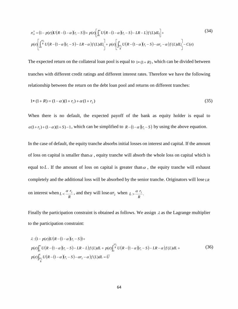
( )( )( ) ( )( )( ) )()(1)()(1)(

)(1)(1)(1

1

211

0 11

2

2

eCdLLfrSrRUepdLLfLRSrRUep

dLLfLLRSrRUepSrRUep

Rr

Rr

SO

−

−−−−−+

−−−−−

+

−−−−−+−−−−=

∫∫

∫

α

α

α

α

ααααα

ααπ

(34)

The expected return on the collateral loan pool is equal to )1(1 R+∗ , which can be divided between

tranches with different credit ratings and different interest rates. Therefore we have the following

relationship between the return on the debt loan pool and returns on different tranches:

)1()1)(1()1(1 21 rrR +++−=+∗ αα (35)

When there is no default, the expected payoff of the bank as equity holder is equal to

1)1)(1()1( 2 −+−++ Sr αα , which can be simplified to ( )( )SrR −−− 11 α by using the above equation.

In the case of default, the equity tranche absorbs initial losses on interest and capital. If the amount

of loss on capital is smaller thanα , equity tranche will absorb the whole loss on capital which is

equal to L . If the amount of loss on capital is greater thanα , the equity tranche will exhaust

completely and the additional loss will be absorbed by the senior tranche. Originators will lose LR

on interest whenRr

L 2α< , and they will lose 2rα when .2

Rr

Lα

>

Finally the participation constraint is obtained as follows. We assign λ as the Lagrange multiplier

to the participation constraint:

( ) ( )( )( )

( )( )( ) ( )( )( )

( )( )( ) UdLLfrSrRUep

dLLfLRSrRUepdLLfLLRSrRUep

SrRUep

Rr

Rr

=−−−−−

+−−−−−+−−−−−

+−−−−

∫∫ ∫

1

21

0 11

1

2

2

)(1)(

)(1)()(1)(

1)(1:

α

α α

α

ααα

ααα

αλ

(36)

64


This constraint ensures the effectiveness of originator’s effort for screening taking into account the

moral hazard problem. By differentiating the originator’s expected utility in the presence of

securitization with respect to screening and monitoring effort (first order condition for choice of

effort), we can calculate the incentive compatibility constraint as follows. We assign µ as the

Lagrange multiplier of this constraint. This constraint is the derivation of the participation

constraint with respect to effort.

( )( )( )( )( )( )

( )( )( ) ( )( )( ) )()(1)()(1)(

)(1)(

1)(:

2

2

1

211

0 1

1


dLLfLLRSrRUep

SrRUep

Rr

Rr ′=−−−−−′+−−−−−′

+−−−−−′

+−−−′−

∫ ∫

∫α

α α

α

ααααα

α

αµ

(37)


This constraint can be applied to ensure that there is no over retention. It excludes 1>α .

=→><→=

≤10101:

αδαδαδ (38)

Optimal securitization contract model

The optimal structured securitization contract with tranching and credit enhancement is attained

by solving the following maximization program:

65

( ) ( )( )( )

( )( )( ) ( )( )( )

( )( )( )

( )( )( )( )( )( )

( )( )( ) ( )( )( )

1:

)()(1)()(1)(

)(1)(

1)(:

)()(1)(

)(1)()(1)(

1)(1:

)()()()()())(1(

2

2

2

2

2

1

211

0 1

1

1

21

0 11

1

1 1

211

≤

′=−−−−−′+−−−−−′

+−−−−−′

+−−−′−

=−−−−−−

+−−−−−+−−−−−

+−−−−

−+−−−−=

∫ ∫

∫

∫∫ ∫

∫ ∫

αδ

ααααα

α

αµ

ααα

ααα

αλ

αααπ

α

αα

α

α

αα

α

αα


dLLfLLRSrRUep

SrRUep

UeCdLLfrSrRUep


SrRUep

dLLfLdLLfrLRepSrMax

Rr

Rr

Rr

Rr

Rr

(39)


First we assume that µ =0 when there is no moral hazard and ∗∗= ee . The investor observes e and

sets its level at the full information level ∗∗e by using the "take it or leave it" strategy. If we

differentiate the design model in (39) with respect to S, we have:

( ) ( )( )

( )( )( ) ( )( )( )

( )( )( ) .0)()1(1)(

)()1(1)()()1(1)(

1))(1()(1)1(:

1

21

0 11

1

2

2

=−−−−−−′

+−−−−−−′+−−−−−−′

+−−−−′−+−−

∫∫ ∫

Rr

Rr

dLLfrSrRUep


SrRUepS

α

α α

α

ααααλ

αααλααλ

ααλα

(40)

By solving the above equation, we can isolateλ

1 as follows:

( ) ( )

( )( )( ) ( )( )( )

( )( )( )∫∫ ∫

−−−−−′

+−−−−−′+−−−−−′

+−−−′−=

1

21

0 11

1

2

2

)(1)(

)(1)()(1)(

))(1()(11

Rr

Rr

dLLfrSrRUep


SrRUep

α

αα

α

ααα

ααα

αλ

(41)

Differentiating the model in (39) with respect toα when µ =0 yields:

66

( ) ( ) ( ) ( ) ( )

( ) ( )

( )( )( )

( )( )( ) .0)()1(1)(

)()1(1)(

)())(1()(

))(1()(1))(1(1)(

1

2121

11

0 11

112

21

2

2

=−−−−−−−−′

+−−−−−−−′

+−−−−−−′

+−−−−′−+−+

−+−−

∫∫

∫

Rr

Rr

dLLfrSrrSrRUep

dLLfSrLRSrRUep

dLLfSrLLRSrRUep

SrSrRUepFepRrFrepSr

α

α

α

α

αααλ

ααλ

αλ

αλαα

(42)

By solving this equation for λ1 , we obtain:

( ) ( ) ( )

( ) ( )

( ) ( )

( ) ( )

( )( )( )

( ) ( )

( )( )( )

( ) ( )

−−

−−−

−−−−−−−−′

+

−−

−−−

−−−−−−−′+

−−

−−−

−−−−−−′

+

−−

−−−

−−−−′−

=

∫

∫∫

))(1(1)(

)()1(1)(

))(1(1)(

)()1(1)(

))(1(1)(

)())(1()(

))(1(1)(

))(1()(1

1

221

1

2121

221

11

221

0 11

221

11

2

2

αα

ααα

αα

αα

αα

α

αα

α

λ

α

α

α

α

FepRr

FrepSr

dLLfrSrrSrRUep

FepRr

FrepSr

dLLfSrLRSrRUep

FepRr

FrepSr

dLLfSrLLRSrRUep

FepRr

FrepSr

SrSrRUep

Rr

Rr

(43)

By equalizing the two equations (41) and (43) together we get the following result:

α =0 solves this equation. We can also verify that Sr >1 at the optimum and calculate the risk

premium (like what it is exactly done in the previous chapter with a modified notation):

premiumriskdLLLfReprS −+−= ∫∗∗ )()1)(( 101

(45)

∫+∗∗ dLLLfRep )()1)(( 10 is the expected loss and the risk premium is equal to (Details are in Appendix

(B.1)):

( )( )( ) ( )( )( )

( )( ) ( ) ( )

( )( )( ) ( )( )( )

−−−−−′+−−−−−′

+−−−−−′+−−−′−

−+

−−

=−−−−−−−′+−−−−−−′

∫∫

∫

∫∫

1

211

0 112

2

1

22121

2

2

2

2

)(1)()(1)(

)())(1()())(1()(1))(1(1

)()1(1)()()(1)(

Rr

Rr

Rr

Rr

dLLfrSrRUepdLLfLRSrRUep

dLLfLLRSrRUepSrRUepF

Rr

Frep

dLLfrrSrRUepdLLfrLRSrRUep

α

α

α

α

α

α

α

ααααα

αααα

ααααα

(44)

67

risk premium ∫ +′′′

−= dLLfRLRURUep )()1(

)()()(

21 221

0

(46)


Now we assume that 0≠µ and there is potential moral hazard. If we differentiate the model in

(39) with respect to S, when 0>µ , we obtain:

( ) ( )( )

( )( )( ) ( )( )( )

( )( )( )

( )( )

( )( )( ) ( )( )( )

( )( )( )0

)()1(1

)()1(1)()1(1)(

1))(1()(

)()1(1

)()1(1)()1(1)(

1))(1()(1)1(:

1

21

0 11

1

1

21

0 11

1

2

2

2

2

=

−−−−−−′

+−−−−−−′+−−−−−−′′

+−−−−′′−

−−−−−−′

+−−−−−−′+−−−−−−′

+−−−−′−+−−

∫∫ ∫

∫∫ ∫

Rr

Rr

Rr

Rr

dLLfrSrRU

dLLfLRSrRUdLLfLLRSrRUep

SrRUep

dLLfrSrRU

dLLfLRSrRUdLLfLLRSrRUep

SrRUepS

α

α α

α

α

α α

α

αααα

αααααµ

ααµ

αααα

αααααλ

ααλα

(47)

By simplifying the above equation, we find:

( ) ( )( )( ) ( )( )( )

( )( )( )

( )))(1(1

)(1

)(1)(1))(1(

)()(1

1

1

21

0 111

2

2

SrRU

dLLfrSrRU

dLLfLRSrRUdLLfLLRSrRUSrRU

epepRr

Rr

−−−′−

−−−−−′

+−−−−−′+−−−−−′+−−−′−

=′+

∫∫ ∫

αλ

ααα

αααα

µλ

α

αα

α

(48)

If we differentiate the model in (39) with respect to α we have:

( ) ( ) ( ) ( ) ( )

( ) ( )

( )( )( )

( )( )( )

( ) ( )

( ) ( )

( )( )( )

( )( )( )

.0

)()1(1

)()1(1

)())(1(

)(

))(1()(

)()1(1

)()1(1

)())(1(

)(

))(1()(1))(1(1)(

1

2121

11

0 11

11

1

2121

11

0 11

112

21

2

2

2

2

=

−−−−−−−−′

+−−−−−−−′

+−−−−−−′

′

+−−−−′′−

−−−−−−−−′

+−−−−−−−′

+−−−−−−′

+−−−−′−+−+

−+−−

∫∫

∫

∫∫

∫

Rr

Rr

Rr

Rr

dLLfrSrrSrRU

dLLfSrLRSrRU

dLLfSrLLRSrRU

ep

SrSrRUep

dLLfrSrrSrRU

dLLfSrLRSrRU

dLLfSrLLRSrRU

ep

SrSrRUepFepRrFrepSr

α

α

α

α

α

α

α

α

ααα

αα

α

µ

αµ

ααα

αα

α

λ

αλαα

(49)

This can be simplified as follow:

68

( ) ( )( )( ) ( )( )( )

( )( )( )

( ) ( )

−+

−−−−−−′−−

−−−−−−−−′

+−−−−−−−′+−−−−−−′+−−−−′−

=′+

∫∫ ∫

))(1(1)())(1()(

)()1(1

)()1(1)()(1)())(1(

)()(1

22111

1

2121

0 111111

2

2

αααλ

ααα

αααα

µλ

α

αα

α

FRrFrepSrSrRUSr

dLLfrSrrSrRU

dLLfSrLRSrRUdLLfSrLLRSrRUSrSrRU

epepRr

Rr

(50)

By equalizing the two equations together we get the following result:

( ) ( )( )( )

( )( )( )

( )( )( )

( ){ }( )( )( )

( )( )( )

+−−−−−′

+−−−−−′−−−′−

=

−−−−−′

+−−−−−′

+−−−−−′+−−−′−

−+

−

∫∫

∫∫

∫

1

221

1

1

1

21

1

0 11

22

2

2

2

2

)()1(1

)(1))(1(1

)(1

)(1

)(1))(1(

))(1(1)(

Rr

Rr

Rr

Rr

dLLfrrSrRU

dLLfLRSrRUSrRU

dLLfrSrRU

dLLfLRSrRU

dLLfLLRSrRUSrRU

FRrFrep

α

α

α

α

α

α

α

ααα

αααλ

ααα

αα

αα

αα

(51)


When there is no moral hazard we have the following particular case:

( )

( )( )( )

( )( )( )( )

( )( )( ) ( )( )( )∫∫

∫∫∫

−−−−−′−−−−−−′

−−−−−−′−

−+

−

+−−−−−′

+−−−−−′

=−−−′−

1

211

0 1

22

1

221

1

1

2

2

2

2

)(1)()(1)(

)())(1()(

))(1(1

)()1(1

)(1

))(1())(1(

Rr

Rr

Rr

Rr


dLLfLLRSrRUep

FRrFr

dLLfrrSrRU

dLLfLRSrRU

SrRUep

α

α

α

αα

α

α

ααααα

α

αα

ααα

αα

α

(52)

We use the following notation to make the above equation simpler:

( )( )( )

( )( )( )

−+

−

+−−−−−′

+−−−−−′

=∫∫

))(1(1

)()1(1

)(1

22

1

221

1

2

2

αα

ααα

αα

α

α

α

FRrFr

dLLfrrSrRU

dLLfLRSrRU

x Rr

Rr

(53)

and

69

( )

( )( )( ) ( )( )( )∫∫

∫−−−−−′+−−−−−′

+−−−−−′=

1

211

0 1

2

2

)(1)()(1)(

)())(1()(

Rr

Rr


dLLfLLRSrRUepy

α

α

α

α

ααααα

α

(54)

Equation (54) becomes:

( ) ( )))(1(

))(1())(1())(1( 11 epyxSrRUyxSrRUep

−−

=−−−′→−=−−−′− αα (55)

With moral hazard we have the following equation using the above notations:

( ) ( )))((

))(1())(1())(( 11 epxyxSrRUyxSrRUepx

−−

=−−−′→−=−−−′−λ

ααλ (56)

To compare (56) with the no moral hazard case, we can write:

x1

=λ , which makes (55) and (56) equivalent.

We now suppose thatx1

<λ . It indicates that ( )))(1( 1 SrRU −−−′ α is higher in (56) than in (55):

( )))(1(

))(1( 1 epyxSrRU

−−

>−−−′ α (57)

Given that U ′ is decreasing in wealth, and, as shown before, Sr >1 , this means that α should be

smaller than or equal to zero to satisfy the inequality. Because α cannot be smaller than zero, this

means that there should be full securitization. By putting 0=α in the above inequality, we get the

following result:

)()( 11 SrRUSrRU −−′>−−′ (58)

which is a contradiction and we reject this possibility. Now considering x1

>λ , we obtain:

( )))(1(

))(1( 1 epyxSrRU

−−

<−−−′ α (59)

70

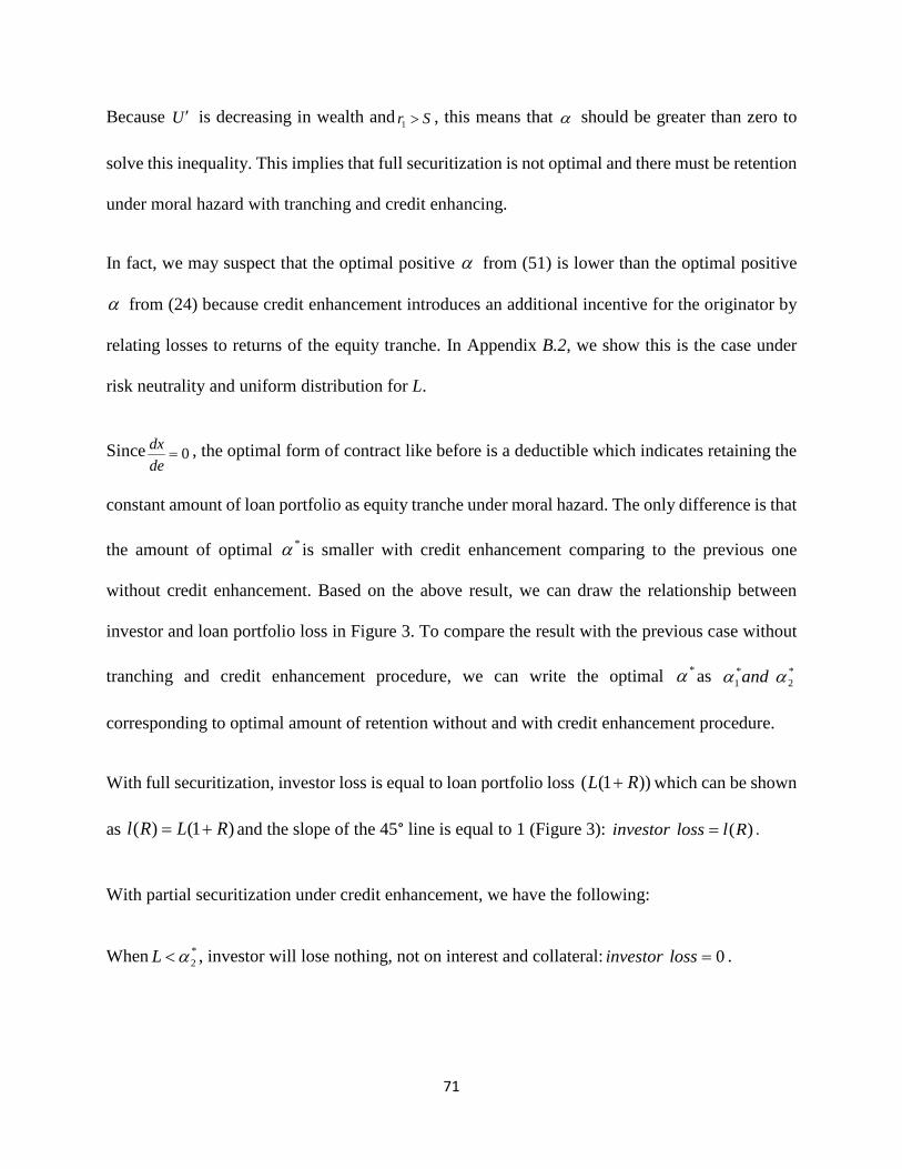
Because U ′ is decreasing in wealth and Sr >1 , this means that α should be greater than zero to

solve this inequality. This implies that full securitization is not optimal and there must be retention

under moral hazard with tranching and credit enhancing.

In fact, we may suspect that the optimal positive α from (51) is lower than the optimal positive

α from (24) because credit enhancement introduces an additional incentive for the originator by

relating losses to returns of the equity tranche. In Appendix B.2, we show this is the case under

risk neutrality and uniform distribution for L.

Since 0=dedx , the optimal form of contract like before is a deductible which indicates retaining the

constant amount of loan portfolio as equity tranche under moral hazard. The only difference is that

the amount of optimal *α is smaller with credit enhancement comparing to the previous one

without credit enhancement. Based on the above result, we can draw the relationship between

investor and loan portfolio loss in Figure 3. To compare the result with the previous case without

tranching and credit enhancement procedure, we can write the optimal *α as *2

*1 αα and

corresponding to optimal amount of retention without and with credit enhancement procedure.

With full securitization, investor loss is equal to loan portfolio loss ))1(( RL + which can be shown

as )1()( RLRl += and the slope of the 45° line is equal to 1 (Figure 3): )(Rllossinvestor = .

With partial securitization under credit enhancement, we have the following:

When *2α<L , investor will lose nothing, not on interest and collateral: 0=lossinvestor .

71

WhenRrL 2*

2*2 αα << , investor will start losing something on collateral, but nothing on interest. In

this case: *2α−= Llossinvestor , which can be rewritten as *

2)1()( α−

+=

RRllossinvestor , compare

to the full securitization, the slope of the line decreased from 1 to )1(

1R+

.

WhenRrL 2*

2α> , investor will lose something both on collateral and interest. In this case:

)1()( 2*2 rRllossinvestor +−= α .

Figure 3: Optimal Securitization Contract under credit enhancement procedure

Investor loss equals 0 when *2α<L , equals )( *

2α−L when RrL 2*

2*2 αα << and equals 2

*2

*2 )( rLRL αα −+− when

RrL 2*

2α>

*2α (Optimal α with credit enhancement) is smaller than *

1α (Optimal α without credit enhancement)(see Appendix B.2) While

Rr2*

2α Could be smaller than or greater than *1α .

Investor loss

0

:

Loan portfolio loss

Full securitization

Partial securitization under credit enhancement

*2α

Partial securitization under moral hazard

*1α

72

3.2 Conditional distribution of loss

In this section, we assume that the originator can affect the distribution function )( eLF and

density function )( eLf of the loss with screening and monitoring effort. In the case of loans default

there is a random conditional loss L which is in the interval [0, 1] : 10 ≤≤ L .

The optimal amount and form of the structured asset-backed securitization contract is obtained by

solving the following maximization program:

( ) ( )( )( )

( )( )( ) ( )( )( )

( )( )( )

( )( )( )( )( )( )

( )( )( ) ( )( )( )

( )( )( ) ( )( )( )

( )( )( )

1:

)()(1)(

)(1)()(1)(

)(1)()(1)(

)(1)(

1)(:

)()(1)(

)(1)()(1)(

1)(1:

)()()()()())(1(

1

21

0 11

1

211

0 1

1

1

21

0 11

1

1 1

211

2

2

2

2

2

2

2

≤

′=−−−−−

+−−−−−+−−−−−

+−−−−−′+−−−−−′

+−−−−−′

+−−−′−

=−−−−−−

+−−−−−+−−−−−

+−−−−

−+−−−−=

∫∫ ∫

∫ ∫

∫

∫∫ ∫

∫ ∫

αδ

ααα

ααα

ααααα

α

αµ

ααα

ααα

αλ

αααπ

α

αα

α

α

αα

α

α

αα

α

αα

eCdLeLfrSrRUep

dLeLfLRSrRUepdLeLfLLRSrRUep

dLeLfrSrRUepdLeLfLRSrRUep

dLeLfLLRSrRUep

SrRUep

UeCdLeLfrSrRUep


SrRUep

dLeLfLdLeLfrLRepSrMax

Rr e

Rr

ee

Rr

Rr

Rr

Rr

Rr

(60)

73

• No Moral Hazard: µ =0



differentiate with respect to S, we have:

( ) ( )( )

( )( )( ) ( )( )( )

( )( )( ) .0)()1(1)(

)()1(1)()()1(1)(

1))(1()(1)1(:

1

21

0 11

1

2

2

=−−−−−−′

+−−−−−−′+−−−−−−′

+−−−−′−+−−

∫∫ ∫

Rr

Rr

dLeLfrSrRUep


SrRUepS

α

αα

α

ααααλ

αααλααλ

ααλα

(61)

By solving the above equation, we can isolate λ1 as follows:

( ) ( )

( )( )( ) ( )( )( )

( )( )( )∫∫ ∫

−−−−−′

+−−−−−−′+−−−−−′

+−−−′−=

1

21

0 11

1

2

2

)(1)(

)()1(1)()(1)(

))(1()(11

Rr

Rr

dLeLfrSrRUep


SrRUep

α

αα

α

ααα

αααα

αλ

(62)

Differentiating with respect toα yields:

( ) ( ) ( ) ( ) ( )

( ) ( )

( )( )( )

( )( )( ) .0)()1(1)(

)()1(1)(

)())(1()(

))(1()(1))(1(1)(

1

2121

11

0 11

112

21

2

2

=−−−−−−−−′

+−−−−−−−′

+−−−−−−′

+−−−−′−+−+

−+−−

∫∫

∫

Rr

Rr

dLeLfrSrrSrRUep

dLeLfSrLRSrRUep

dLeLfSrLLRSrRUep

SrSrRUepFepRr

FrepSr

α

α

α

α

αααλ

ααλ

αλ

αλαα

(63)


74

( ) ( ) ( )

( ) ( )

( ) ( )

( ) ( )

( )( )( )

( ) ( )

( )( )( )

( ) ( )

−−

−−−

−−−−−−−−′

+

−−

−−−

−−−−−−−′+

−−

−−−

−−−−−−′

+

−−

−−−

−−−−′−

=

∫

∫∫

))(1(1)(

)()1(1)(

))(1(1)(

)()1(1)(

))(1(1)(

)())(1()(

))(1(1)(

))(1()(1

1

221

1

2121

221

11

221

0 11

221

11

2

2

αα

αααλ

αα

αα

αα

α

αα

α

λ

α

α

α

α

FepRr

FrepSr

dLeLfrSrrSrRUep

FepRr

FrepSr

dLeLfSrLRSrRUep

FepRr

FrepSr

dLeLfSrLLRSrRUep

FepRr

FrepSr

SrSrRUep

Rr

Rr

(64)


( )( )( ) ( )( )( )

( )( ) ( ) ( )

( )( )( ) ( )( )( )

−−−−−′+−−−−−′

+−−−−−′+−−−′−

−+

−−

=−−−−−−−′+−−−−−−′

∫∫

∫

∫∫

1

211

0 112

2

1

2211

2

2

2

2

)(1)()(1)(

)())(1()())(1()(1))(1(1

)()1(1)()()1(1)(

Rr

Rr

Rr

Rr


dLeLfLLRSrRUepSrRUepF

Rr

Frep

dLeLfrrSrRUepdLeLfLRSrRUep

α

α

α

α

α

α

α

ααααα

αααα

ααααα

(65)

α =0 solves this equation.

75


Now we assume that 0≠µ and there is potential moral hazard. If we differentiate the model with

respect to S, we have:

( ) ( )( )

( )( )( ) ( )( )( )

( )( )( )

( )( )

( )( )( ) ( )( )( )

( )( )( )

( )( )( ) ( )( )( )

( )( )( )0

)()1(1

)()1(1)()1(1)(

)()1(1

)()1(1)()1(1)(

1))(1()(

)()1(1

)()1(1)()1(1)(

1))(1()(1)1(:

1

21

0 11

1

21

0 11

1

1

21

0 11

1

2

2

2

2

2

2

=

−−−−−−′

+−−−−−−′+−−−−−−′+

−−−−−−′

+−−−−−−′+−−−−−−′′

+−−−−′′−

−−−−−−′

+−−−−−−′+−−−−−−′

+−−−−′−+−−

∫∫ ∫

∫∫ ∫

∫∫ ∫

Rr e

Rr

ee

Rr

Rr

Rr

Rr

dLeLfrSrRU

dLeLfLRSrRUdLeLfLLRSrRUep

dLeLfrSrRU


SrRUep

dLeLfrSrRU


SrRUepS

α

αα

α

α

αα

α

α

αα

α

αααα

αααααµ

αααα

αααααµ

ααµ

αααα

αααααλ

ααλα

(66)


( ) ( )( )( ) ( )( )( )

( )( )( )

( )( )( )( ) ( )( )( )

( )( )( )

−−−−−′

+−−−−−′+−−−−−′−−−−′−

−−−−−′

+−−−−−′+−−−−−′+−−−′−

=′+

∫∫ ∫

∫∫ ∫

1

21

0 11

1

1

21

0 111

2

2

2

2

)(1

)(1)(1)())(1(1

)(1

)(1)(1))(1(

)()(1

Rr e

Rr

ee

Rr

Rr

dLeLfrSrRU

dLeLfLRSrRUdLeLfLLRSrRUepSrRU

dLeLfrSrRU

dLeLfLRSrRUdLeLfLLRSrRUSrRU

epep

α

αα

α

α

αα

α

ααα

αααµαλ

ααα

αααα

µλ

(67)

If we differentiate with respect to α we have:

( ) ( ) ( ) ( ) ( )

( ) ( )

( )( )( )

( )( )( )

( ) ( )

( ) ( )

( )( )( )

( )( )( )

( ) ( )

( )( )( )

( )( )( )

0

)()1(1

)()1(1

)())(1(

)(

)()1(1

)()1(1

)())(1(

)(

))(1()(

)()1(1

)()1(1

)())(1(

)(

))(1()(1))(1(1)(

1

2121

11

0 11

1

2121

11

0 11

11

1

2121

11

0 11

112

21

2

2

2

2

2

2

=

−−−−−−−−′

+−−−−−−−′

+−−−−−−′

+

−−−−−−−−′

+−−−−−−−′

+−−−−−−′

′

+−−−−′′−

−−−−−−−−′

+−−−−−−−′

+−−−−−−′

+−−−−′−+−+

−+−−

∫∫

∫

∫∫

∫

∫∫

∫

Rr e

Rr

e

e

Rr

Rr

Rr

Rr

dLeLfrSrrSrRU

dLeLfSrLRSrRU

dLeLfSrLLRSrRU

ep

dLeLfrSrrSrRU

dLeLfSrLRSrRU

dLeLfSrLLRSrRU

ep

SrSrRUep

dLeLfrSrrSrRU

dLeLfSrLRSrRU

dLeLfSrLLRSrRU

ep

SrSrRUepFepRr

FrepSr

α

α

α

α

α

α

α

α

α

α

α

α

ααα

αα

α

µ

ααα

αα

α

µ

αµ

ααα

αα

α

λ

αλαα

(68)

76


( ) ( )( )( ) ( )( )( )

( )( )( )

( ) ( )

( )( )( ) ( )( )( )

( )( )( )

−−−−−−−−′

+−−−−−−−′+−−−−−−′−

−+

−−−−−−′−−

−−−−−−−−′

+−−−−−−−′+−−−−−−′+−−−−′−

=′+

∫∫ ∫

∫∫ ∫

1

2121

0 1111

22111

1

2121

0 111111

2

2

2

2

)()1(1

)()1(1)()(1)(

))(1(1)())(1()(

)()1(1

)()1(1)()(1)())(1(

)()(1

Rr e

Rr

ee

Rr

Rr

dLeLfrSrrSrRU

dLeLfSrLRSrRUdLeLfSrLLRSrRUep

FRrFrepSrSrRUSr

dLeLfrSrrSrRU

dLeLfSrLRSrRUdLeLfSrLLRSrRUSrSrRU

epep

α

αα

α

α

αα

α

ααα

αααµ

αααλ

ααα

αααα

µλ

(69)


( ) ( )( )( )

( )( )( )

( )( )( )

( )( )( ) ( )( )( )

( ){ }( )( )( )

( )( )( )

+−−−−−′

+−−−−−′−−−′−+

+−−−−−′+−−−−−′

=

−−−−−′

+−−−−−′

+−−−−−′+−−−′−

−+

−

∫∫

∫ ∫

∫∫

∫

1

221

1

1

1

2211

1

21

1

0 11

22

2

2

2

2

2

2

)()1(1

)(1))(1(1

)()1(1)(1)(

)(1

)(1

)(1))(1(

))(1(1)(

Rr

Rr

Rr

Rr ee

Rr

Rr

dLeLfrrSrRU

dLeLfLRSrRUSrRU

dLeLfrrSrRUdLeLfLRSrRUep

dLeLfrSrRU

dLeLfLRSrRU

dLeLfLLRSrRUSrRU

FRrFrep

α

α

α

α

αα

α

α

α

α

ααα

αααλ

αααααµ

ααα

αα

αα

αα

(70)

77


We use the following notations to make the comparison possible:

( )( )( )

( )( )( )

( )

( )( )( ) ( )( )( )∫∫

∫

∫∫

−−−−−′+−−−−−′

+−−−−−′=

−+

−

+−−−−−′

+−−−−−′

=

1

211

0 1

22

1

221

1

2

2

2

2

)(1)()(1)(

)())(1()(

))(1(1

)()1(1

)(1

Rr

Rr

Rr

Rr


dLeLfLLRSrRUepy

FRrFr

dLeLfrrSrRU

dLeLfLRSrRU

x

α

α

α

α

α

α

α

ααααα

α

αα

ααα

αα

(71)

When there is no moral hazard we have the following equation using the above notations:

( ) ( )))(1(

))(1())(1())(1( 11 epyxSrRUyxSrRUep

−−

=−−−′→−=−−−′− αα (72)

With moral hazard we have the following equation using above notations:

( ) ( )))(()())(1()())(1())(( 11 epxxepyxSrRUxepyxSrRUepx e

e −+−

=−−−′→+−=−−−′−λ

µαµαλ (73)

To compare the moral hazard case with the no moral hazard one (equations (73) and (72)

correspondingly) and get the global maximum contract to obtain the optimalα , we impose MLRP

(Monotone Likelihood Ratio Property) (see Winter (2000)). MLRP is a property of the ratio)()(

eLfeLfe

when )( eLf is a probability density function and )( eLfe is the derivative of )( eLf with respect

to e . We need to make an assumption about the sign of

)()(

eLfeLf

dLd e to obtain an optimal solution.

Its sign depends on L and the ratio can be >, = or < than 0. Moreover the sign of MLRP changes

78

as L changes. To make an assumption possible we need to analyze the sign of ex . In the following

analysis we consider 4 cases to make a correct assumption:

First we assume that x1

<λ and 0<ex :

In this case the comparison between equations (72) and (73) is impossible, since at the same time

both numerator and the denominator of equation (73) decreases.

Second we assume that x1

<λ and 0>ex :

In this case since the numerator of equation (73) increases and its denominator decreases,

( )))(1( 1 SrRU −−−′ α is increasing:

( )))(1(

))(1( 1 epyxSrRU

−−

>−−−′ α (74)

Since U ′ is decreasing in wealth under risk aversion and as shown before Sr >1 this means that α

must be smaller than or equal to zero to satisfy the inequality. Since α cannot be smaller than

zero, this means that there should be full securitization. By putting 0=α in the above inequality,

we get the following result:

)()( 11 SrRUSrRU −−′>−−′ (75)

Which is a contradiction and we reject this possibility.

Now considering the third case, where x1

>λ and 0>ex :

In this case the comparison is again impossible, since at the same time both numerator and the

denominator of equation (73) increase.

79

Finally we consider the fourth case, where x1

>λ and 0<ex :

In this case since the numerator of equation (73) decreases and its denominator increases, therefore

( )))(1( 1 SrRU −−−′ α is decreasing:

( )))(1(

))(1( 1 epyxSrRU

−−

<−−−′ α (76)



under moral hazard. The optimal solution is 0* >α . In Appendix B.3, we show that under risk

neutrality and exponential distribution for L, ex will be negative which means that these

assumptions are satisfactory to get the result.

The structure of ex determines the structure of the contract. In the previous section when we had

tranching but an unconditional distribution of loss, ex was equal to zero:

( )( )( )

( )( )( )0,

))(1(1

)()1(1

)(1

22

1

221

1

2

2

=

−+

−

+−−−−−′

+−−−−−′

=∫∫

dedx

FRrFr

dLLfrrSrRU

dLLfLRSrRU

x Rr

Rr

αα

ααα

αα

α

α

α

(77)

Because MLRP is constant in that case, therefore the optimal form of the contract indicated

retaining the constant amount of loan portfolio as equity tranche (retention) which was positive

and could be calculated based on the model.

With tranching and conditional distribution of loss, the optimal solution corresponds to the fourth

case (which is the only acceptable case). In the fourth case we have 0<ex , where:

80

( )( )( )

( )( )( )0

))(1(1

)()1(1

)(1

22

1

221

1

2

2

<

−+

−

+−−−−−′

+−−−−−′

==∫∫

αα

ααα

αα

α

α

α

FRrFr

dLeLfrrSrRU

dLeLfLRSrRU

dedxx R

r e

Rr

e

e

(78)

The numerator is representing the loss of the senior tranche, this means that with effort, originator

could decrease the loss of the senior tranche (investor). On the other hand the bank will decrease

the density function by maximizing the effort level which is consistent with the investors’

objective. As a result (like in Winter (2000)) we assume that 0)()(

<

eLfeLf

dLd e , because as L increases

)( eLfe moves from >0 to <0. To obtain the best contract, we want that the ratio decreases when

L increases. Therefore the optimal form of contract in this case, suggesting keeping a fraction of

senior tranches as proportional retention (or coinsurance in insurance literature) in addition to the

equity tranche retention as before (fixed amount retention as a deductible).

With conditional distribution of loss, as shown in fourth case, since 0<dedx , the optimal form of

contract is different from unconditional distribution of loss: the fixed amount of equity retention

plus a fraction of higher losses as proportional retention. In Figure 4, we can draw the relationship

between investor and loan portfolio loss based on the above results. As for a coinsurance contract

the bank’s exposure to risk increases with L.

81

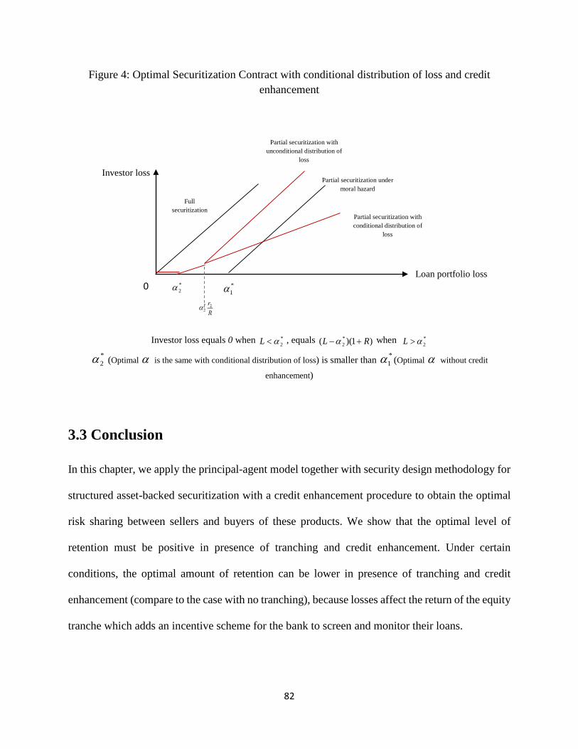
Figure 4: Optimal Securitization Contract with conditional distribution of loss and credit enhancement

Investor loss equals 0 when *

2α<L , equals )1)(( *2 RL +−α when *

2α>L *2α (Optimal α is the same with conditional distribution of loss) is smaller than *

1α (Optimal α without credit

enhancement)

3.3 Conclusion

In this chapter, we apply the principal-agent model together with security design methodology for

structured asset-backed securitization with a credit enhancement procedure to obtain the optimal

risk sharing between sellers and buyers of these products. We show that the optimal level of

retention must be positive in presence of tranching and credit enhancement. Under certain

conditions, the optimal amount of retention can be lower in presence of tranching and credit

enhancement (compare to the case with no tranching), because losses affect the return of the equity

tranche which adds an incentive scheme for the bank to screen and monitor their loans.

Investor loss

0

Loan portfolio loss

Full securitization

Partial securitization with unconditional distribution of

loss

*2α

Partial securitization under moral hazard

*1α

Partial securitization with conditional distribution of

loss

82

The optimal form of retention can be different with conditional and unconditional distribution of

loss. With unconditional distribution of loss, the optimal form of contract is equity tranche

retention, while with conditional distribution of loss it will be proportional to the total loss, which

indicates fixed amount of equity tranche plus a fraction of higher losses as coinsurance. The

optimal amount of retention in both cases is the same while the optimal form of retention would

be different.

The main intuition of our results is the following1(Malekan and Dionne (2014 )): To reduce the

default possibility and ensure the investor’s participation incentive, the originator chooses his

effort and the security price before the uncertainty is realized. Because the security price is

determined in the ex-ante situation, the originator is not given any incentive to choose an

appropriate effort level if it does not hold an equity tranche or vertical slice of all the tranches.

However, if the originator holds an equity tranche or vertical slice of all the tranches, it must partly

incur the default loss. As a result, the existence of the retention part gives the originator an

incentive to reduce the default probability to avoid incurring the default loss.

However, if the equity tranche retention or proportional retention requirements are too high,

securitization may no longer be an economical form of acquiring liquidity from the financial

market because it could cause unintended costs and consequently impede efforts to restart

sustainable securitization markets (Selody and Woodman, 2009). Therefore, it becomes critical to

select an appropriate amount and form of tranche retention based on precise calculations, which

was the focus of our research. The optimal amount and form of tranche retention could then be

calculated using our model with different parameter values.

1 We thank a referee for suggesting this interpretation.

83

A recent empirical study (Casu, Clare, Sarkisyan and Thomas (2011 )) shows that securitization

reduces bank credit risk taking. But the authors admit that this negative effect can be offseted by

the risk arising from the securitized pool. Our contribution shows explicitly how optimal tranche

retention in securitization may reduce the securitized pool risk by increasing the incentives for

banks to monitor their loans. Consequently, the offsetting effect discussed by (Casu, Clare,

Sarkisyan and Thomas (2011 )) can be non-significant when optimal risk-sharing contracts of

securitization are put in place.

For future research, we will take one step further by considering structured asset-backed

securitization with a credit enhancement procedure in the presence of correlation between assets

in the original pool, as observed during the recent financial crisis.

84

Chapter 4:

Structured Asset-backed Securitization with Systemic Risk

http://en.wikipedia.org/wiki/Structured_finance

http://en.wikipedia.org/wiki/Asset-backed_security

Introduction

In this chapter we take one step further by considering structured asset-backed securitization with

credit enhancement procedure in the presence of the endogenous correlation on return between

assets in the original pool. In other words, we assume that there is a systemic risk in this section.

By letting the size of the loan pool to be large enough, we could diversify away the idiosyncratic

risk. But the return on the loan pool does not depend only on the loan-specific factor which

constitutes idiosyncratic risks that could be diversified away by choosing a large size of the loan

pool. It also depends on common factors like macroeconomic conditions that affect the entire

underlying portfolio at the same time. These factors constitute the systemic risk which leads to

correlation between the default risks of underlying loans and consequently different tranches.

These correlations were not considered before the recent financial crisis, which led to

underestimation of true default probabilities of tranches in the presence of systemic risk. This also

resulted in the inaccurate rating and pricing of the financial products associated with different

tranches.

Because of these correlations, this kind of risk cannot be diversified away easily and brings about

more default risk than has been anticipated. That is why it becomes important to take into account

the systemic risk when determining the credit risk and accordingly the rating of the entire loan

pool. Systemic risk does increase the chance of many loans defaulting at the same time.

The more the correlation between defaults risks of different tranches, the more the value of the

equity tranche. Thus the value of equity tranche increases with more correlation. The value of

senior tranche may fall dramatically with correlation. The outcome of correlation on the value of

86

the mezzanine tranche is mixed; it depends on factors like the relative tranche size (Coval, Jurek

and Stafford (2009)).

The objective here is to compute the optimal amount and form of retention under moral hazard

and systemic risk and to compare the impact of systemic risk on the optimal amount of retention

without systemic risk.

4.1 Derivation of the model

We consider a risk-averse originator or bank who detains a loan pool with a value normalized to

1. The loan pool is assumed to be large enough to diversify away the idiosyncratic risk but systemic

risk which leads to correlation between the defaults risks of different loans cannot be diversified

away and brings about more default risk than has been anticipated. We suppose that the average

default probability of loan pool without systemic risk is )(ep which is a function of screening and

monitoring effort .e Effort e could be undertaken by lenders to decrease the probability of loans

default. We assume )(ep is decreasing and convex in effort:

.0)(,0)( >′′<′ epep (80)

Effort is costly for originators. The cost function is equal to )(eC and is increasing and convex ine :

0)(,0)(,0)0( >′′>′= eCeCC (81)

In the case of loans default there is a random conditional loss L which is in the interval [0, 1]:

10 ≤≤ L . )(LF is the distribution function of loss, conditional on having default with density

function )(Lf . )(Lf is not a function of effort in this section.

87

The risk-free rate of interest is normalized to zero. Originator securitizes some part of the loan

pool as senior tranches to risk-neutral and competitive investors. The amount of senior tranches

which are securitized is equal to α−1 with higher credit rating than the average of the loan pool

and a lower interest rate of 1r . The originator can keep α fraction of the loan pool as equity tranche

with lower credit rating and interest rate 2r higher than 1r .

Because of the systemic risk there is a correlation between default probabilities of different assets

in the underlying loan pool. Systemic risk can be interpreted as domino effect in the default

probability of underlying assets. In other words, if one loan defaults, the probability that other

loans defaults increases because of systemic risk. We can explain the effect of systemic risk on

default probabilities by an example. Let us assume a loan pool with two identical securities — call

them “bonds”—both of which have a default probability of 10% and a zero recovery rate. They are

securitized with two tranches as junior (B) and senior (A).The junior tranche defaults if either loan

defaults, while the senior tranche defaults only if both loans default.

If we assume that the two loans are uncorrelated, the default probability of the senior tranche is

1% (10% x 10%)! That of the junior tranche is 19% (10% + 90% x 10%)! We can use )(BPN and

)(APN to identify default probability of junior and senior tranche respectively when there is no

systemic risk.

)(APN = 1%

)(BPN =19%

(82)

88

If both are correlated the default probability of the junior and the senior tranches are calculated as

below, which can be identified by )(BPS and )(APS respectively while there is systemic risk:

)(APS = 1%+ρ10%(1-10%) > )(APN

)(BPS = 19%-ρ10%(1-10%) < )(BPN

(83)

Here ρ is the correlation coefficient. As shown in the above example, the presence of dependence

increases the default probability of senior tranche )()( APAP NS > while at the time decreases that

of junior tranche )()( BPBP NS < . In other words, the systemic transfer of the junior tranche risk to

senior tranche is a function of correlation coefficient. The increment is a product of the correlation

coefficient ρ and the probability that senior tranche defaults.

In our model, the default probability of senior and junior tranches with systemic risk can be shown

as P(A) and P(B) respectively:

))(()()( BPgepAP ρ+=

))(()()( BPgepBP ρ−=

(84)

We assume that effort cannot affect ρ which is a natural assumption. Therefore, similar to the

example, in presence of systemic risk the default probability of the senior tranche will increase as

a function of the correlation coefficient (ρ) and the probability that the senior tranche defaults. The

89

junior tranche absorbs the first part of the loss on interest and capital. Senior tranche can participate

in the default probability of the junior tranche as a function of correlation which was shown before.

As a result, the return of investors will increase correspondingly. Since they absorb the ρ fraction

of the loss which was previously incurred by equity trancheα , their return increases as a ρ

fraction ofα .


The expected return of investors is equal to:

−+−−−−= ∫ ∫

1 1

211 2)()()()()())(1(

Rr LfLdLLfrLRAPSr α α

αααπ (85)

In the non-default state the return of investors is equal to )1)(1( 1r+−α . If the loan pool defaults,

the α fraction that is kept by the originator absorbs initial losses both on interest and capital. So

the investors lose something if the amount of loss on interest or capital or both will be large enough

to exhaust the equity tranche.

Investors will lose something on interest when: 2* rRLoss α> or when Rr

Loss 2α> , and the

amount they will lose is equal to ( )2rLR α− which is the amount that is not absorbed by equity

tranche, therefore investors’ expected loss on interest is equal to:

∫ −1

22)()(

Rr dLLfrLRα α (86)

Investors will lose something on capital when: α>Loss and the amount that they will lose is

equal to )( α−L . The expected loss on capital is equal to:

90

dLLfL∫ −1

)()(α

α (87)

The amount that investors are willing to pay for the securitized loan is equal to their expected value

of their payoff which is equal to: )1()1( S+−α . It is the expected rate of return on the loan pool by

considering the potential default risk of the loan pool. With full securitization, when 0=α , the

expected profit of investor is equal to:

∫ +−−≡ dLLfRLAPSrI )()1()()( 101π (88)


In order to satisfy the participation constraint, the expected utility of originator in the presence of

securitization should be at least equal to U . U is the best opportunity when considering

securitization. In case of securitization, we can write the expected utility of originator as follows:

( ) ( )( )( ) ( )( )( )

( )( )( ) ( )( )( )

−−−−−+

−−−−−

+

−−−−−+−−−−

∫∫

∫1

211

0 11

2

2

)(1)()(1)(

)(1)(1)(1

Rr

Rr

dLLfrSrRUBPdLLfLRSrRUBP

dLLfLLRSrRUBPSrRUBP

α

α

α

α

ααααα

αα

(89)

The expected return on the collateral loan pool when there is no default is equal to: )1(1 R+∗ that

can be divided between tranches with different credit rating and different interest rate. Therefore

we have the following relationship between return on collateral loan pool and return on different

tranches:

)1()1)(1()1(1 21 rrR +++−=+∗ αα (90)

When there is no default the expected payoff of equity holder is equal to 1)1)(1()1( 2 −+−++ Sr αα

that can be simplified by using the above equation to ( )( )SrR −−− 11 α .

91

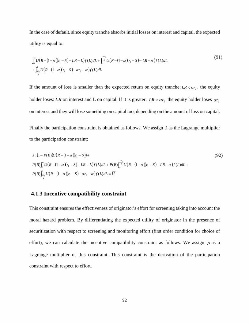
In the case of default, since equity tranche absorbs initial losses on interest and capital, the expected

utility is equal to:

( )( )( ) ( )( )( )

( )( )( )∫∫ ∫

−−−−−+

−−−−−+−−−−−1

21

0 11

2

2

)(1

)(1)(1

Rr

Rr

dLLfrSrRU

dLLfLRSrRUdLLfLLRSrRU

α

αα

α

ααα

ααα (91)

If the amount of loss is smaller than the expected return on equity tranche: 2rLR α< , the equity

holder loses: LR on interest and L on capital. If it is greater: 2rLR α> the equity holder loses 2rα

on interest and they will lose something on capital too, depending on the amount of loss on capital.

Finally the participation constraint is obtained as follows. We assign λ as the Lagrange multiplier

to the participation constraint:

( ) ( )( )( )

( )( )( ) ( )( )( )

( )( )( ) UdLLfrSrRUBP

dLLfLRSrRUBPdLLfLLRSrRUBP

SrRUBP

Rr

Rr

=−−−−−

+−−−−−+−−−−−

+−−−−

∫∫ ∫

1

21

0 11

1

2

2

)(1)(

)(1)()(1)(

1)(1:

α

αα

α

ααα

ααα

αλ

(92)


This constraint ensures the effectiveness of originator’s effort for screening taking into account the

moral hazard problem. By differentiating the expected utility of originator in the presence of

securitization with respect to screening and monitoring effort (first order condition for choice of

effort), we can calculate the incentive compatibility constraint as follows. We assign µ as a

Lagrange multiplier of this constraint. This constraint is the derivation of the participation

constraint with respect to effort.

92

( )( )( )( )( )( )

( )( )( ) ( )( )( ) )()(1)()(1)(

)(1)(

1)(:

2

2

1

211

0 1

1

eCdLLfrSrRUBPdLLfLRSrRUBP

dLLfLLRSrRUBP

SrRUBP

Rr

Rr ′=−−−−−′+−−−−−′

+−−−−−′

+−−−′−

∫ ∫

∫α

αα

α

ααααα

α

αµ

(93)


This constraint is applied to ensure that there is no over retention excluding 1>α .

=→><→=

≤10101:

αδαδαδ (94)

Optimal securitization contract model

The optimal form of the structured asset-backed securitization contract is attained by solving the

following maximization program:

( ) ( )( )( )

( )( )( ) ( )( )( )

( )( )( )

( )( )( )

( )( )( )

( )( )( ) ( )( )( )

1:

)()(1)()(1)(

)(1)(

1)(:

)()(1)(

)(1)()(1)(

1)(1:

)()()()()())(1(

2

2

2

2

2

1

211

0 1

1

1

21

0 11

1

1 1

211

≤

′=−−−−−′+−−−−−′

+−−−−−′

+−−−′−

=−−−−−−

+−−−−−+−−−−−

+−−−−

−+−−−−=

∫ ∫

∫

∫∫ ∫

∫ ∫

αδ

ααααα

α

αµ

ααα

ααα

αλ

αααπ

α

αα

α

α

αα

α

αα

eCdLLfrSrRUBPdLLfLRSrRUBP

dLLfLLRSrRUBP

SrRUBP

UeCdLLfrSrRUBP


SrRUBP

dLLfLdLLfrLRAPSrMax

Rr

Rr

Rr

Rr

Rr

(95)


93



differentiate the design model in (95) with respect to S, we have:

( ) ( )( )

( )( )( ) ( )( )( )

( )( )( ) .0)()1(1)(

)()1(1)()()1(1)(

1))(1()(1)1(:

1

21

0 11

1

2

2

=−−−−−−′

+−−−−−−′+−−−−−−′

+−−−−′−+−−

∫∫ ∫

Rr

Rr

dLLfrSrRUBP


SrRUBPS

α

αα

α

ααααλ

αααλααλ

ααλα

(96)

By solving the above equation, we can isolateλ

1 as follows:

( ) ( )

( )( )( ) ( )( )( )

( )( )( )∫∫ ∫

−−−−−′

+−−−−−′+−−−−−′

+−−−′−=

1

21

0 11

1

2

2

)(1)(

)(1)()(1)(

))(1()(11

Rr

Rr

dLLfrSrRUBP


SrRUBP

α

αα

α

ααα

ααα

αλ

(97)

Differentiating the model in (95) with respect toα when µ =0 yields:

( ) ( ) ( )

( ) ( )

( )( )( )

( )( )( ) .0)()1(1)(

)()1(1)(

)())(1()(

))(1()(1))(1)((1)()(

1

2121

11

0 11

112

21

2

2

=−−−−−−−−′

+−−−−−−−′

+−−−−−−′

+−−−−′−+−+

−+−−

∫∫

∫

Rr

Rr

dLLfrSrrSrRUBP

dLLfSrLRSrRUBP

dLLfSrLLRSrRUBP

SrSrRUBPFAPRrFrAPSr

α

α

α

α

αααλ

ααλ

αλ

αλαα

(98)


94

( ) ( ) ( )

( ) ( ) ( )( )( )

( )( )( )

−−

−−−

−−−−−−−−′

+

−−

−−−

−−−−−−−′+

−−

−−−

−−−−−−′

+

−−

−−−

−−−−′−

=

∫

∫∫

))(1)((1)()(

)()1(1)(

))(1)((1)()(

)()1(1)(

))(1)((1)()(

)())(1()(

))(1)((1)()(

))(1()(1

1

221

1

2121

221

11

221

0 11

221

11

2

2

αα

ααα

αα

αα

αα

α

αα

α

λ

α

α

α

α

FAPRr

FrAPSr

dLLfrSrrSrRUBP

FAPRr

FrAPSr

dLLfSrLRSrRUBP

FAPRr

FrAPSr

dLLfSrLLRSrRUBP

FAPRr

FrAPSr

SrSrRUBP

Rr

Rr

(99)

By equalizing the two equations (97) and (99) together we get the following result:

α =0 solves this equation only when )()( BPAP = which is equivalent to 0=ρ in our model. While

10 << ρ , full securitization is no more an optimal solution even when there is no moral hazard.

( )( )( ) ( )( )( )

( ) ( ) ( )

( )( )( ) ( )( )( )

−−−−−′+−−−−−′

+−−−−−′+−−−′−

−+

−−

=−−−−−−−′+−−−−−−′

∫∫

∫

∫∫

1

211

0 112

2

1

2211

2

2

2

2

)(1)()(1)(

)())(1()())(1()(1))(1(1)(

)()1(1)()()1(1)(

Rr

Rr

Rr

Rr

dLLfrSrRUBPdLLfLRSrRUBP

dLLfLLRSrRUBPSrRUBPF

Rr

FrAP

dLLfrrSrRUBPdLLfLRSrRUBP

α

α

α

α

α

α

α

ααααα

αααα

ααααα

(100)

95


Now we assume that 0≠µ and there is potential moral hazard. If we differentiate (95) with respect

to S, when 0>µ , we obtain:

( ) ( )( )

( )( )( ) ( )( )( )

( )( )( )

( )( )

( )( )( ) ( )( )( )

( )( )( )0

)()1(1

)()1(1)()1(1)(

1))(1()(

)()1(1

)()1(1)()1(1)(

1))(1()(1)1(:

1

21

0 11

1

1

21

0 11

1

2

2

2

2

=

−−−−−−′

+−−−−−−′+−−−−−−′′

+−−−−′′−

−−−−−−′

+−−−−−−′+−−−−−−′

+−−−−′−+−−

∫∫ ∫

∫∫ ∫

Rr

Rr

Rr

Rr

dLLfrSrRU

dLLfLRSrRUdLLfLLRSrRUBP

SrRUBP

dLLfrSrRU

dLLfLRSrRUdLLfLLRSrRUBP

SrRUBPS

α

αα

α

α

αα

α

αααα

αααααµ

ααµ

αααα

αααααλ

ααλα

(101)


( ) ( )( )( ) ( )( )( )

( )( )( )

( )))(1(1

)(1

)(1)(1))(1(

)()(1

1

1

21

0 111

2

2

SrRU

dLLfrSrRU

dLLfLRSrRUdLLfLLRSrRUSrRU

BPBPRr

Rr

−−−′−

−−−−−′

+−−−−−′+−−−−−′+−−−′−

=′+

∫∫ ∫

αλ

ααα

αααα

µλ

α

αα

α

(102)

If we differentiate equation (95) with respect to α we have:

( ) ( ) ( )

( ) ( )

( )( )( )

( )( )( )

( ) ( )

( ) ( )

( )( )( )

( )( )( )

.0

)()1(1

)()1(1

)())(1(

)(

))(1()(

)()1(1

)()1(1

)())(1(

)(

))(1()(1))(1)((1)()(

1

2121

11

0 11

11

1

2121

11

0 11

112

21

2

2

2

2

=

−−−−−−−−′

+−−−−−−−′

+−−−−−−′

′

+−−−−′′−

−−−−−−−−′

+−−−−−−−′

+−−−−−−′

+−−−−′−+−+

−+−−

∫∫

∫

∫∫

∫

Rr

Rr

Rr

Rr

dLLfrSrrSrRU

dLLfSrLRSrRU

dLLfSrLLRSrRU

BP

SrSrRUBP

dLLfrSrrSrRU

dLLfSrLRSrRU

dLLfSrLLRSrRU

BP

SrSrRUBPFAPRrFrAPSr

α

α

α

α

α

α

α

α

ααα

αα

α

µ

αµ

ααα

αα

α

λ

αλαα

(103)


96

( ) ( )( )( ) ( )( )( )

( )( )( )

( )

−+

−−−−−−′−−

−−−−−−−−′

+−−−−−−−′+−−−−−−′+−−−−′−

=′+

∫∫ ∫

))(1(1)()())(1()(

)()1(1

)()1(1)()(1)())(1(

)()(1

22111

1

2121

0 111111

2

2

αααλ

ααα

αααα

µλ

α

αα

α

FRrFrAPSrSrRUSr

dLLfrSrrSrRU

dLLfSrLRSrRUdLLfSrLLRSrRUSrSrRU

BPBPRr

Rr

(104)


( ) ( )( )( )

( )( )( )

( )( )( )

( ){ }( )( )( )

( )( )( )

+−−−−−′

+−−−−−′−−−′−

=

−−−−−′

+−−−−−′

+−−−−−′+−−−′−

−+

−

∫∫

∫∫

∫

1

221

1

1

1

21

1

0 11

22

2

2

2

2

)()1(1

)(1))(1(1

)(1

)(1

)(1))(1(

))(1(1)(

Rr

Rr

Rr

Rr

dLLfrrSrRU

dLLfLRSrRUSrRU

dLLfrSrRU

dLLfLRSrRU

dLLfLLRSrRUSrRU

FRrFrAP

α

α

α

α

α

α

α

ααα

αααλ

ααα

αα

αα

αα

(105)


When there is no moral hazard we have the following particular case:

( )

( )( )( )

( )( )( )( )

( )( )( ) ( )( )( )∫∫

∫∫∫

−−−−−′−−−−−−′

−−−−−−′−

−+

−

+−−−−−′

+−−−−−′

=−−−′−

1

211

0 1

22

1

221

1

1

2

2

2

2

)(1)()(1)(

)())(1()(

))(1(1)(

)()1(1

)(1)(

))(1())(1(

Rr

Rr

Rr

Rr

dLLfrSrRUBpdLLfLRSrRUBp

dLLfLLRSrRUBp

FRrFrAP

dLLfrrSrRU

dLLfLRSrRUBP

SrRUBp

α

α

α

αα

α

α

ααααα

α

αα

ααα

αα

α

(106)

We use the following notation to make the above equation simpler:

( )( )( )

( )( )( )

−+

−

+−−−−−′

+−−−−−′

=∫∫

))(1(1)(

)()1(1

)(1)(

22

1

221

1

2

2

αα

ααα

αα

α

α

α

FRr

FrAP

dLLfrrSrRU

dLLfLRSrRUBP

x Rr

Rr

(107)

and

97

( )

( )( )( ) ( )( )( )∫∫

∫−−−−−′+−−−−−′

+−−−−−′=

1

211

0 1

2

2

)(1)()(1)(

)())(1()(

Rr

Rr

dLLfrSrRUBpdLLfLRSrRUBp

dLLfLLRSrRUBpy

α

α

α

α

ααααα

α (108)

Equation (108) becomes:

( ) ( )))(1(

))(1())(1())(1( 11 BpyxSrRUyxSrRUBp

−−

=−−−′→−=−−−′− αα (109)

With moral hazard we have the following equation using the above notations:

( ) ( )))((

))(1())(1())(( 11 BpxyxSrRUyxSrRUBpx

−−

=−−−′→−=−−−′−λ

ααλ (110)

To compare (110) with the no moral hazard case, we can write:

x1

=λ , which makes (109) and (110) equivalent.

We now suppose thatx1

<λ . It indicates that ( )))(1( 1 SrRU −−−′ α is higher in (110) than in (109):

( )))(1(

))(1( 1 BpyxSrRU

−−

>−−−′ α (111)

Given that U ′ is decreasing in wealth, and, as shown before, Sr >1 this means that α should be

smaller than or equal to zero to satisfy the inequality. Because α cannot be smaller than zero, this

means that there should be full securitization. By putting 0=α in the above inequality, we get the

following result:

)()( 11 SrRUSrRU −−′>−−′ (112)

which is a contradiction and we reject this possibility. Now considering x1

>λ , we obtain:

( )))(1(

))(1( 1 BpyxSrRU

−−

<−−−′ α (113)

98



under moral hazard with tranching and systemic risk.

In fact, we may suspect that the optimal positive α from (105) is greater than the optimal positive

α from (51). Because of the systemic risk, some part of the default probability of equity tranche

which is held by the bank will transfer to investors. This reduction in default probability decreases

bank’s exposure to the risk. Therefore we need an additional incentive for the bank to maintain its

effort at a high level by increasing the amount of retention. In Appendix C.1, we show this is the

case under risk neutrality and uniform distribution for L.

When 0=ρ , the optimal amount of retention from (105) is the same as the optimal amount of

retention from (51) with no systemic risk and unconditional distribution of loss. But when

10 << ρ , the optimal amount of retention with systemic risk is greater than the optimal amount

of retention with no systemic risk. Therefore an increase in optimal retention can offset the extra

insecurity which is the result of systemic risk.

So far, we show that the systemic risk resulted in an increase of optimal amount of retention. But

what is not obvious yet is that if this increase in the optimal amount of retention should be out of

junior tranche or senior tranche. As we mentioned in previous chapter, the sign of ex determines

the structure of the contract. In the previous section when we had tranching but an unconditional

distribution of loss, ex was equal to zero:

99

( )( )( )

( )( )( )0,

))(1(1

)()1(1

)(1

22

1

221

1

2

2

=

−+

−

+−−−−−′

+−−−−−′

=∫∫

dedx

FRrFr

dLLfrrSrRU

dLLfLRSrRU

x Rr

Rr

αα

ααα

αα

α

α

α

(114)

Because MLRP is constant in that case, therefore the optimal form of the contract indicated

retaining the constant amount of loan portfolio as equity tranche (deductible) which was positive

and could be calculated based on the model.

With tranching and systemic risk, we have 0<ex (details are in Appendix C.2), where:

( )( )( )

( )( )( )0

))(1(1)(

)()1(1

)(1)(

))()(

)()(

(2

2

1

221

1

2

2

<

−+

−

+−−−−−′

+−−−−−′

−==∫∫

αα

ααα

αα

α

α

α

FRrFrAP

dLLfrrSrRU

dLLfLRSrRUBP

APAP

BPBP

dedxx R

r

Rr

eee

(115)

The numerator is representing the loss of the senior tranche, this means that with effort, originator

could decrease the loss of the senior tranche (investor). Therefore the optimal form of contract in

this case, suggesting keeping a fraction of senior tranches as proportional retention in addition to

the equity tranche as before (fixed amount retention as a deductible).

With systemic risk, since 0<dedx , the optimal form of contract is different from tranching and

unconditional distribution of loss, may be it suggests to keep some part of mezzanine tranche; the

fixed amount retention of equity plus a fraction of other tranches as coinsurance. In Figure 5, we

can draw the relationship between investor and loan portfolio loss based on the above results.

100

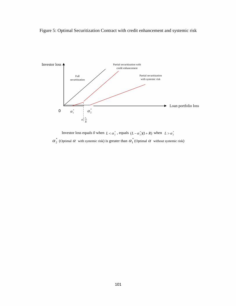
Figure 5: Optimal Securitization Contract with credit enhancement and systemic risk

Investor loss equals 0 when *

2α<L , equals )1)(( *2 RL +−α when *

2α>L *2α (Optimal α with systemic risk) is greater than *

1α (Optimal α without systemic risk)

Investor loss

0

Loan portfolio loss

Full securitization

Partial securitization with credit enhancement

*1α *

2α

Partial securitization with systemic risk

101

4.2 Conclusion

In this chapter, we take one step further by considering structured asset-backed securitization with

a credit enhancement procedure in the presence of correlation between tranches in the original

pool, as observed during the recent financial crisis.

These correlations were not considered by market participants before and during the recent

financial crisis, which led to underestimation of the true default probabilities of all tranches in the

presence of systemic risk. This also resulted in an inaccurate rating of structured financial products

associated with different tranches (Dionne (2009)).

Because of extra insecurity which is the outcome of systemic risk, the optimal amount of retention

should increase to the point that to offset this extra insecurity. The correlation between defaults

risks of different assets in the original pool transfer some part of the default risk of junior tranche

which is held by the bank to investors. It can be interpreted that in this case the default probability

of the bank reduced as a function of correlation coefficient. In order to keep the incentive of the

bank at the optimal level, we need to increase the amount of retention to the point that by

considering this transfer, bank will exert the first best effort as previous case with no systemic risk.

The optimal form of the contract indicates that increase in optimal amount of retention should be

out of senior tranches. One reason for this could be the fact that since default risk of junior tranche

transfer to senior tranche, if we would like to increase the amount of retention out of junior tranche,

the optimal amount of retention should increase too much. As we mentioned before too much

retention can offset the advantage of securitization.

102

This result is consistent with (Fender and Mitchell (2009b)). Because the equity tranche will be

exhausted when there is a large probability of a systemic risk. It could decrease the originator’s

incentive to make a screening effort. In this case it would be better to hold also mezzanine tranche

(Fender and Mitchell (2009b)).

A recent empirical study (Casu et al, 2011) shows that securitization reduces bank credit risk-

taking. However, the authors admit that this negative effect can be offset by the risk arising from

the securitized pool. Our contribution explicitly shows how an optimal tranche in securitization

may reduce the securitized pool risk by increasing banks’ incentives to monitor their loans.

Consequently, the offsetting effect discussed by Casu et al (2011) can be non-significant when

optimal risk-sharing contracts of securitization are put in place.

103

Appendix

Appendix A

A.1 Second-order condition

The second-order condition is negative at the optimum: ( ) 0, ( ) 0′′ ′′> >C e p e and (1 )− + <R L R R

implies that ( )1

0(1 ) ( ) ( )− + −∫ U R L R f L dL U R is negative. As a result we verify the negativity of the

S.O.C:

1

0( ) ( ) ( (1 )) ( ) ( ) 0.∗∗ ∗∗ ′′ ′′− + − + − < ∫C e p e U R L R f L dL U R (A.1)

A.2 Risk premium when there is no moral hazard

We can verify that R>S and by calculating the difference between R and S we can calculate the

risk premium. From the participation constraint we have the following:

( ) ( )

( ) ( )1

0

1 ( ) (1 )( )

(1 )( ) (1 ) ( ) ( (1 )( ) (1 )) ( ) ( ).

= − − − − +

− − − − + + − − − − + − ∫ ∫α

α

α

α α α

U p e U R R S

p e U R R S L R f L dL U R R S R f L dL C e (A.2)

When there is no securitization (α =0), the originator will exert the first best effort level ∗∗e , and

the right-hand side of the above equation is equal to:

( ) ( ).∗∗−U S C e (A.3)

The originator’s expected utility without securitization while the originator exerts the first best

effort is equal to:

104

( ) ( )101 ( ) ( ) ( ) (1 ) ( ) ( ).∗∗ ∗∗ ∗∗− + − + −∫p e U R p e U R L R f L dL C e (A.4)

Equalizing these two equations yields the following equality from the participation constraint:

( ) ( )1

0( ) ( ) 1 ( ) ( ) ( ) (1 ) ( ) ( ).∗∗ ∗∗ ∗∗ ∗∗− = − + − + −∫U S C e p e U R p e U R L R f L dL C e (A.5)

We can calculate the risk premium by applying a Taylor expansion around R to both sides of

equation (A.5). The Taylor expansion of the left side of this equation is equal to:

The Taylor expansion of the right side of equation (A.5) is equal to:

( ) ( ) ( )1 1 22

0 01 ( ) ( ) ( ) ( ) ( ) 1 ( ) ( ) ( ) 1 ( ) .

2′′ ′− + − + + + ∫ ∫

Up e U R p e U R p e L R f L dL U R p e L R f L dL (A.7)

Equalizing these two equations yields the following:

1 1 2 2

0 0

1 ( )( )(1 ) ( ) ( ) (1 ) ( ) ( )2 ( )

′′= − + + +

′∫ ∫U RS R p e R Lf L dL p e L R f L d LU R

(A.8)

where the risk premium = 1 2 20

1 ( )( ) (1 ) ( ) .2 ( )

′′− +

′ ∫U Rp e L R f L dLU R

(A.9)

Under risk aversion, the risk premium is positive because ( ) 0, ( ) 0, ( ) 0′′ ′> < >p e U R U R .Therefore,

we can conclude that R-S is larger than the expected loss. The expected return of originator is then

equal to:

1 1 2 2

0 0

1 ( )1 1 ( ) ( ) (1 ) ( ) (1 ) ( ) ( ).2 ( )

′′ + = − + + + ′∫ ∫U RS p e Lf L dL R p e L R f L d LU R

(A.10)

( ) ( ) ( ) ( ).′= + −U S U R S R U R (A.6)

105

Appendix B

B.1 Risk premium

We can verify that Sr >1 and by calculating the difference between 1r and S we can calculate the

risk premium. From the participation constraint we have the following:

(B.1)

When there is no securitization α =0, the originator will exert the first best effort level ∗∗e , and the

above equation is equal to:

)()( 1∗∗−+−= eCSrRUU (B.2)

On the other hand, U is equal to the expected utility of originator without securitization while

originator exerts the first best effort:

[ ] [ ] )()())1(( )()()(1 10

∗∗∗∗∗∗ −+−+−= ∫ eCdLLfRLRUepRUePU (B.3)

By putting these two equations equal we have the following equality:

[ ] )()())1(()()())(1(()()( 101

∗∗∗∗∗∗∗∗ −+−+−=−+− ∫ eCdLLfRLRUepRUepeCSrRU (B.4)

Now, we have to show that:

premiumriskdLLLfReprS .)()1)(( 101 −+−= ∫∗∗ (B.5)

We can calculate the risk premium by applying a Taylor expansion around R to both sides of above

equation. The Taylor expansion of the left side of this equation is equal to:

)()()()( 11 RUrSRUSrRU ′−+=+− (B.6)

The Taylor expansion of the right side of equation is equal to:

( ) ( )( )( )

( )( )( ) ( )( )( )

( )( )( ) )()(1)(

)(1)()(1)(

1)(1

1

21

0 211

1

2

2

eCdLLfrSrRUep

dLLfLrSrRUepdLLfLLRSrRUep

SrRUepU

Rr

Rr

−−−−−−

+−−−−−+−−−−−

+−−−−=

∫

∫ ∫

α

ααα

ααα

ααα

α

106

[ ] [ ]2

)()1()()()()1()()()()())(1(( 2210

10

UdLLfRLepRUdLLfRLepRUepRUep′′

++′+−+− ∫∫ (B.7)

By putting these two equations equal we have the following:

∫∫ +′′′

++−=1

0

221

01 )()()1()()()(

21)()1)(( LdLfRL

RURUepdLLLfReprS (B.8)

Where the ∫ +′′′

−= dLLfRLRURUeppremiumrisk )()1(

)()()(

21 221

0 (B.9)

The risk premium is positive; because: 0)(,0)(,0)( >′<′′> RURUep ,Therefore, we can conclude that

Sr >1 .

107

B.2 Risk neutrality case

We want to show there is substitution between α and 2r for the bank in presence of tranching and

credit enhancement. For certain levels of 2,r optimal α can be lower when there is tranching

because losses reduce 2r for the bank and creates an additional incentive for screening and

monitoring the loans under moral hazard. Differentiating (39) with respect to α and S yields the

following equilibrium condition, assuming risk neutrality ( ( ) 1)′ =U x and uniform distribution for

L in the interval [0, 1]. The two first order conditions are as follow:

If we differentiate the model in (39) with respect to S we have:

( ) 10)()()()(11: =⇒=′+′−+−+− λµµλλ epepepepS (B.10)


( ) ( ) ( ) ( )

( ) ( ) 01)()1)(()()(

1)()1)(())(()(1)1(1)(:

2211

2211

221

=

−′−−′−−′+−′−

−−−−−+−−+−+

−+−−

Rr

eprepSrepSrep

Rr

eprepSrepSrepepRr

repSr

αµαµµµ

αλαλλλααα (B.11)


0)1)(()1(2

22 =−+−−− ααµλ

Rrrep

(B.12)

Since 1=λ and 0≠µ , It is easy to obtain an explicit value ofα :

01

12

2

2 >

+

+=

Rrrα under moral hazard. (B.13)

108

Differentiating (B.13) with respect to 2r :

222

22

21.

)1()1(

+

+−+=

RrR

rRdrdα

(B.14)

Since )1()1( 22 Rr +>+ then

2drdα < 0.

This means that a high 2r can be a substitute to a highα , so a lower α can be sufficient to maintain

the incentives in presence of credit enhancement when there is tranching.

109

B.3 Conditional distribution

We assume risk neutrality and negative exponential distribution for L. First, we need to calculate

ex to make sure if these are satisfactory assumptions.

Loss distribution function:

ee

e

LLeLF

LeLF−

−

=

=

))(ln()(

)(

(B.15)

Plus risk neutrality:

ee

ee

e

Rrrr

Rr

Rrr

dedxx

−−

−−

−+−

−−==

αα

αααα

1)(

)ln()()ln(

222

222

(B.16)

Since , the numerator is positive but the denominator is negative, which means .

Since 0<ex , is the necessary condition to get the result under conditional distribution of loss, it

means that these assumptions are satisfactory to get the result.

10 2 <<Rrα 0<ex

110

Appendix C

C.1 Risk neutrality case

We want to show that the optimal amount of retention will increase in the presence of systemic

risk, because systemic risk will introduce more uncertainty about the underlying loan pool. With

systemic risk the default probability of junior tranche decreases at the cost of an increase in the

default probability of senior tranche. In this case we expect that the return on the equity tranche (

2r ) decreases as a result of decrease in its default probability. Therefore if we can show there is a

negative substitution between α and 2r in presence of systemic risk, we can show that optimal

amount of α increases (due to decrease in 2r which is the result of systemic risk).

Differentiating (95) with respect to α and S yields the following equilibrium condition, assuming

risk neutrality ( ( ) 1)′ =U x and uniform distribution for L in the interval [0,1]. The two first order

conditions, are as follows:

If we differentiate the model in (95) with respect to S we have:

( ) 10)()()()(11: =⇒=′+′−+−+− λµµλλ BpBpBpBpS (C.1)


( ) ( ) ( ) ( )

( ) ( ) 01)()1)(()()(

1)()1)(())(()(1)1(1)(:

2211

2211

221

=

−′−−′−−′+−′−

−−−−−+−−+−+

−+−−

Rr

BprBpSrBpSrBp

Rr

BprBpSrBpSrBpApRr

rApSr

αµαµµµ

αλαλλλααα (C.2)


111

( ) 0)1()()()(2

22 =−+−′−− ααµλ

RrrBpBpAp (C.3)

In this case we can obtain an explicit value ofα :

01

12

2

2 >

+

+=

Rrrα under moral hazard. (C.4)

Differentiating (C.2) with respect to 2r :

222

22

21.

)1()1(

+

+−+=

RrR

rRdrdα

(C.5)

Since )1()1( 22 Rr +>+ then

2drdα < 0.

This means that the reduction in 2r due to systemic risk can be interpreted as an increase in optimal

α to maintain the originator’s incentives at the optimal level to take care about it.

112

C.2 optimal contract structure based on the sign of the ex

We have the following equation for x with tranching and systemic risk:

( )( )( )

( )( )( )

−+

−

+−−−−−′

+−−−−−′

=∫∫

))(1(1)(

)()1(1

)(1)(

22

1

221

1

2

2

αα

ααα

αα

α

α

α

FRr

FrAP

dLLfrrSrRU

dLLfLRSrRUBP

x Rr

Rr

(C.6)

ex can be calculated as below:

( )( )( )

( )( )( )0

))(1(1)(

)()1(1

)(1)(

))()(

)()((

22

1

221

1

2

2

<

−+

−

+−−−−−′

+−−−−−′

−==∫∫

αα

ααα

αα

α

α

α

FRrFrAP

dLLfrrSrRU

dLLfLRSrRUBP

APAP

BPBP

dedxx R

r

Rr

eee

(C.7)

We can show that ex is negative:

The second part of the above equation is positive, to show that ex is negative, we need to show that the first part is negative:

)()())((

)()())(()

)(1

)(1)((

)()())(()(

)()())(()(

)()(

)()(

APBPBPf

BPBPBPf

APBPep

APBPBPfep

BPBPBPfep

APAP

BPBP ee

′′−

′′−−′

=′′+′

−′′−′

=−

ρρ

ρρ

(C.8)

Since )()( BPAP > then )(

1)(

1APBP

> . We know that 0)( <′ ep so 0))(

1)(

1)(( <−′APBP

ep . As a result

0<ex .

113

References Akerlof, George A, 1970, The market for" lemons": Quality uncertainty and the market

mechanism, The Quarterly Journal of Economics 488-500. Albertazzi, Ugo, Ginette Eramo, Leonardo Gambacorta, and Carmelo Salleo, 2011, Securitization

is not that evil after all, AFA 2012 Chicago Meetings Paper. Allen, Franklin, and Elena Carletti, 2006, Credit risk transfer and contagion, Journal of Monetary

Economics 53, 89-111. Altunbas, Yener, Leonardo Gambacorta, and David Marques-Ibanez, 2009, Securitisation and the

bank lending channel, European Economic Review 53, 996-1009. Ambrose, Brent, Michael LaCour-Little, and Anthony Sanders, 2003, Does regulatory capital

arbitrage or asymmetric information drive securitization, Unpublished Manuscript. Angelides, Phil, and Bill Thomas, 2011. The financial crisis inquiry report: Final report of the

national commission on the causes of the financial and economic crisis in the united states (revised corrected copy) (Government Printing Office).

Antonio, Nicolo', and Loriana Pelizzon, 2005, Credit derivatives: Capital requirements and

strategic contracting, (Dipartimento di Scienze Economiche" Marco Fanno"). Ashcraft, Adam B, and Til Schuermann, 2008. Understanding the securitization of subprime

mortgage credit (Now Publishers Inc). Axelson, Ulf, 2007, Security design with investor private information, The Journal of Finance 62,

2587-2632. Ayotte, Kenneth M, and Stav Gaon, 2005, Asset-backed securities: Costs and benefits of

“bankruptcy remoteness, Columbia Business School. Barth, Mary E, Gaizka Ormazabal, and Daniel J Taylor, 2011, Asset securitizations and credit risk,

The Accounting Review 87, 423-448. Batty, David Line, 2011, Dodd-frank's requirement of skin in the game for asset-backed securities

may scalp corporate loan liquidity, NC Banking Inst. 15, 13. Berndt, Antje, and Anurag Gupta, 2009, Moral hazard and adverse selection in the originate-to-

distribute model of bank credit, Journal of Monetary Economics 56, 725-743. Best, Ronald, and Hang Zhang, 1993, Alternative information sources and the information content

of bank loans, The Journal of Finance 48, 1507-1522.

114

Billett, Matthew T, Mark J Flannery, and Jon A Garfinkel, 2006, Are bank loans special? Evidence on the post-announcement performance of bank borrowers, Journal of Financial and Quantitative Analysis 41, 733-751.

Bolton, Patrick, and Mathias Dewatripont, 2005. Contract theory (MIT press). Boot, Arnoud WA, and Anjan V Thakor, 1993, Security design, The Journal of Finance 48, 1349-

1378. Brunnermeier, Markus K, 2008, Deciphering the liquidity and credit crunch 2007-08, (National

Bureau of Economic Research). Calomiris, Charles W, and Joseph R Mason, 2004, Credit card securitization and regulatory

arbitrage, Journal of Financial Services Research 26, 5-27. Carey, Mark, Stephen Prowse, John Rea, and Gregory Udell, 1994, Economics of the private

placement market, the, Fed. Res. Bull. 80, 5. Casu, Barbara, Andrew Clare, Anna Sarkisyan, and Stephen Thomas, 2011, Does securitization

reduce credit risk taking? Empirical evidence from us bank holding companies, The European Journal of Finance 17, 769-788.

Chen, Weitzu, Chi-Chun Liu, and Stephen G Ryan, 2008, Characteristics of securitizations that

determine issuers' retention of the risks of the securitized assets, The Accounting Review 83, 1181-1215.

Cheng, Mei, Dan S Dhaliwal, and Monica Neamtiu, 2011, Asset securitization, securitization

recourse, and information uncertainty, The Accounting Review 86, 541-568. Chiesa, Gabriella, 2008, Optimal credit risk transfer, monitored finance, and banks, Journal of

Financial Intermediation 17, 464-477. Colander, David, Michael Goldberg, Armin Haas, Katarina Juselius, Alan Kirman, Thomas Lux,

and Brigitte Sloth, 2009, The financial crisis and the systemic failure of the economics profession, Critical Review 21, 249-267.

Coval, Joshua, Jakub Jurek, and Erik Stafford, 2009, The economics of structured finance, The

Journal of Economic Perspectives 3-26. Dahiya, Sandeep, Manju Puri, and Anthony Saunders, 2003, Bank borrowers and loan sales: New

evidence on the uniqueness of bank loans*, The Journal of Business 76, 563-582. Dang, Tri Vi, Gary Gorton, and Bengt Holmstrom, 2009, Opacity and the optimality of debt for

liquidity provision, Manuscript Yale University.

115

De Bandt, Olivier, and Philipp Hartmann, 2000, Systemic risk: A survey, Available at SSRN 258430.

Dell’Ariccia, Giovanni, Deniz Igan, and Luc Laeven, 2012, Credit booms and lending standards:

Evidence from the subprime mortgage market, Journal of Money, Credit and Banking 44, 367-384.

DeMarzo, Peter, and Darrell Duffie, 1999, A liquidity‐based model of security design,

Econometrica 67, 65-99. DeMarzo, Peter M, 2005, The pooling and tranching of securities: A model of informed

intermediation, Review of Financial Studies 18, 1-35. Demyanyk, Yuliya, and Otto Van Hemert, 2011, Understanding the subprime mortgage crisis,

Review of Financial Studies 24, 1848-1880. Diamond, Douglas W, 1984, Financial intermediation and delegated monitoring, The Review of

Economic Studies 51, 393-414. Diamond, Douglas W, and Philip H Dybvig, 1983, Bank runs, deposit insurance, and liquidity,

The economics of structured finance, The Journal of Political Economy 401-419. Diamond, Douglas W, and Raghuram Rajan, 2009, The credit crisis: Conjectures about causes and

remedies, (National Bureau of Economic Research). Diamond, Douglas W, and Raghuram G Rajan, 2009, Illiquidity and interest rate policy, (National

Bureau of Economic Research). Dionne, Georges, 2009, Structured finance, risk management, and the recent financial crisis, Ivey

Business Journal, 7 p. Dionne, Georges, and Tarek M Harchaoui, 2008, Banks' capital, securitization and credit risk: An

empirical evidence for Canada, Insurance and Risk Management 75, 459-485. Donnelly, Catherine, and Paul Embrechts, 2010, The devil is in the tails: Actuarial mathematics

and the subprime mortgage crisis, Astin Bulletin 40, 1-33. Downing, Chris, Dwight Jaffee, and Nancy Wallace, 2009, Is the market for mortgage-backed

securities a market for lemons?, Review of Financial Studies 22, 2457-2494. Drucker, Steven, and Christopher Mayer, 2008, Inside information and market making in

secondary mortgage markets, Manuscript, Columbia University. Drucker, Steven, and Manju Puri, 2009, On loan sales, loan contracting, and lending relationships,

Review of Financial Studies 22, 2835-2872.

116

http://ssrn.com/abstract=258430

Dugan,John.C., 2010,February 2, Securitization,‘skin-in-the-game’ proposals, and minimum mortgage underwriting standards. Remarks before the American Securitization Forum. Retrieved, from http://www.occ.gov/news- issuances/speeches/2010/pub-speech-2010-13.pdf.

Ellul, Andrew, and Vijay Yerramilli, 2013, Stronger risk controls, lower risk: Evidence from us

bank holding companies, The Journal of Finance 68, 1757-1803. Elul, Ronel, 2011, Securitization and mortgage default, Available at SSRN 1484973. Estrella, Arturo, 2002, Securitization and the efficacy of monetary policy, Economic Policy Review

8, 243-255. Fender, Ingo, and Janet Mitchell, 2009a, The future of securitisation: How to align incentives?,

BIS Quarterly Review 3, 25-50. Fender, Ingo, and Janet Mitchell, 2009b, Incentives and tranche retention in securitisation: A

screening model, National Bank of Belgium Working Paper 177 (2009). Firla-Cuchra, Maciej, and Tim Jenkinson, 2005, Security design in the real world: Why are

securitization issues tranched? Working Paper, Oxford University. Freixas, Xavier, and Jean-Charles Rochet. Microeconomics of banking. Vol. 2. Cambridge, MA:

MIT press, 1997. Gale, Douglas, and Martin Hellwig, 1985, Incentive-compatible debt contracts: The one-period

problem, The Review of Economic Studies 52, 647-663. Gambacorta, Leonardo, and David Marques‐Ibanez, 2011, The bank lending channel: Lessons

from the crisis, Economic Policy 26, 135-182. Gande, Amar, Manju Puri, Anthony Saunders, and Ingo Walter, 1997, Bank underwriting of debt

securities: Modern evidence, Review of Financial Studies 10, 1175-1202. Gande, Amar, and Anthony Saunders, 2012, Are banks still special when there is a secondary

market for loans?, The Journal of Finance 67, 1649-1684. Gennaioli, Nicola, Andrei Shleifer, and Robert Vishny, 2012, Neglected risks, financial

innovation, and financial fragility, Journal of Financial Economics 104, 452-468. Gibbons, Robert, and Kevin J Murphy, 1991, Relative performance evaluation for chief executive

officers, (National Bureau of Economic Research). Glaeser, Edward L, and Hedi D Kallal, 1997, Thin markets, asymmetric information, and

mortgage-backed securities, Journal of Financial Intermediation 6, 64-86.

117

http://dx.doi.org/10.2139/ssrn.1484973

Gorton, Gary B, 2008, The panic of 2007, (National Bureau of Economic Research). Gorton, Gary B, 2009, Information, liquidity, and the (ongoing) panic of 2007, (National Bureau

of Economic Research). Gorton, Gary B, 2010. Slapped by the invisible hand: The panic of 2007 (Oxford University Press). Gorton, Gary B, and George G Pennacchi, 1995, Banks and loan sales marketing nonmarketable

assets, Journal of monetary Economics 35, 389-411. Gorton, Gary B, and Nicholas S Souleles, 2007, Special purpose vehicles and securitization, in

The risks of financial institutions (University of Chicago Press). Gorton, Gary, and Andrew Metrick, 2012, Securitization, (National Bureau of Economic

Research). Goswami, Mangal, Andreas A Jobst, and Xin Long, 2009, An investigation of some macro-

financial linkages of securitization, Available at SSRN 1345576. Greenbaum, Stuart I, and Anjan V Thakor, 1987, Bank funding modes: Securitization versus

deposits, Journal of Banking & Finance 11, 379-401. Gupta, Anurag, Ajai K Singh, and Allan A Zebedee, 2008, Liquidity in the pricing of syndicated

loans, Journal of Financial Markets 11, 339-376. Haensel, Dennis, and Jan Pieter Krahnen, 2007, Does credit securitization reduce bank risk?

Evidence from the european cdo market, Evidence from the European CDO Market (January 29, 2007).

Hart, Oliver, and Bengt Holmstrom, 2008, A theory of firm scope, (National Bureau of Economic

Research). Hartman-Glaser, Barney, Tomasz Piskorski, and Alexei Tchistyi, 2012, Optimal securitization

with moral hazard, Journal of Financial Economics 104, 186-202. Hellwig, Martin F, 2009, Systemic risk in the financial sector: An analysis of the subprime-

mortgage financial crisis, De Economist 157, 129-207. Higgins, Eric J, and Joseph R Mason, 2004, What is the value of recourse to asset-backed

securities? A clinical study of credit card banks, Journal of Banking & Finance 28, 875-899.

Hölmstrom, Bengt, 1979, Moral hazard and observability, The Bell Journal of Economics 74-91. Holmstrom, Bengt, and Jean Tirole, 1997, Financial intermediation, loanable funds, and the real

sector, the Quarterly Journal of economics 663-691.

118

Innes, Robert D, 1990, Limited liability and incentive contracting with ex-ante action choices,

Journal of Economic Theory 52, 45-67. Jeon, Haejun, and Michi Nishihara, 2012, Securitization under asymmetric information and risk

retention requirement, Available at SSRN 2116770. Kashyap, Anil K, and Jeremy C Stein, 2000, What do a million observations on banks say about

the transmission of monetary policy?, American Economic Review 407-428. Kendall, Leon T, and Michael J Fishman, 2000. A primer on securitization (MIT press). Keys, Benjamin J, Tanmoy K Mukherjee, Amit Seru, and Vikrant Vig, 2008, Did securitization

lead to lax screening? Evidence from subprime loans, EFA 2008 Athens Meetings Paper. Keys, Benjamin J, Tanmoy Mukherjee, Amit Seru, and Vikrant Vig, 2009, Financial regulation

and securitization: Evidence from subprime loans, Journal of Monetary Economics 56, 700-720.

Kiff, John, and Michael Kisser, 2010. Asset securitization and optimal retention (International

Monetary Fund). Kothari, SP, Elena Loutskina, and Valeri V Nikolaev, 2006, Agency theory of overvalued equity

as an explanation for the accrual anomaly, Available at SSRN 871750. Kroszner, Randall S, and Raghuram G Rajan, 1994, Is the glass-steagall act justified? A study of

the us experience with universal banking before 1933, The American Economic Review 810-832.

Kuttner, Kenneth, 2000, Securitization and monetary policy, Unpublished paper, Federal Reserve

Bank of New York. Leland, E Hayne, and David H Pyle, 1977, Informational asymmetries, financial structure, and

financial intermediation, The journal of Finance 32, 371-387. Levitin, Adam J, 2013, Skin-in-the-game: Risk retention lessons from credit card securitization,

The George Washington Law Review 81, 813. Loutskina, Elena, 2006, The role of securitization in bank financial management, Federal Reserve

Bank of Chicago Proceedings. Loutskina, Elena, 2011, The role of securitization in bank liquidity and funding management,

Journal of Financial Economics 100, 663-684.

119

http://papers.ssrn.com/sol3/papers.cfm?abstractid-1093137%23%23

Loutskina, Elena, and Philip E Strahan, 2009, Securitization and the declining impact of bank finance on loan supply: Evidence from mortgage originations, The Journal of Finance 64, 861-889.

Lummer, Scott L, and John J McConnell, 1989, Further evidence on the bank lending process and

the capital-market response to bank loan agreements, Journal of Financial Economics 25, 99-122.

Malekan, Sara, and Georges Dionne, 2014, Securitization and optimal retention under moral

hazard, Journal of Mathematical Economics 55, 74-85. Mian, Atif, and Amir Sufi, 2008, The consequences of mortgage credit expansion: Evidence from

the 2007 mortgage default crisis, (National Bureau of Economic Research). Minton, Bernadette, Anthony Sanders, and Philip E Strahan, 2004, Securitization by banks and

finance companies: Efficient financial contracting or regulatory arbitrage? Working Paper, Ohio State University.

Morgenson, Gretchen, and Louise Story, 2010, Rating agency data aided wall street in deals, New

York Times. Morrison, Alan D, 2005, Credit derivatives, disintermediation, and investment decisions, The

Journal of Business 78, 621-648. Niu, Flora F, and Gordon D Richardson, 2006, Are securitizations in substance sales or secured

borrowings? Capital‐market evidence, Contemporary Accounting Research 23, 1105-1133.

Osano, Hiroshi, 1999, Security design, insider monitoring, and financial market equilibrium,

European Finance Review 2, 273-302. Paligorova, Teodora, 2009, Agency conflicts in the process of securitization, Bank of Canada

Review 2009, 36-50. Park, Sunyoung, 2013, The design of subprime mortgage-backed securities and information

insensitivity, International Economic Journal 27, 249-284. Parlour, Christine A, and Guillaume Plantin, 2008, Loan sales and relationship banking, The

Journal of Finance 63, 1291-1314. Parlour, Christine A, and Andrew Winton, 2013, Laying off credit risk: Loan sales versus credit

default swaps, Journal of Financial Economics 107, 25-45. Pavel, Christine, and David Phillis, 1987, Why commercial banks sell loans: An empirical

analysis, Federal Reserve Bank of Chicago Economic Perspectives 14, 3-14.

120

Pennacchi, George G, 1988, Loan sales and the cost of bank capital, The Journal of Finance 43, 375-396.

Plantin, Guillaume, 2004, Tranching. London school of economics, (Working Paper April,

London). Rajan, Raghuram G, 2006, Has finance made the world riskier?, European Financial Management

12, 499-533. Rajan, Uday, Amit Seru, and Vikrant Vig, 2010, The failure of models that predict failure:

Distance, incentives and defaults, Chicago GSB Research Paper. Riddiough, Timothy J, 1997, Optimal design and governance of asset-backed securities, Journal

of Financial Intermediation 6, 121-152. Rosenkranz, Robert, 2009, Let’s write the rating agencies out of our law, Wall Street Journal

(January 2). Selody, Jack, and Elizabeth Woodman, 2009, Reform of securitization, Financial System Review

47-52. Shleifer, Andrei, and Robert W Vishny, 2010, Unstable banking, Journal of Financial Economics

97, 306-318. Sorkin, Andrew, 2009, Too big to fail: The inside story of how wall street and washington fought

to save the financial system, (Penguin Group. New York, NY: Penguin Group). Stein, Jeremy C, 2002, Information production and capital allocation: Decentralized versus

hierarchical firms, The Journal of Finance 57, 1891-1921. Stein, Jeremy C, 2011, Monetary policy as financial-stability regulation, (National Bureau of

Economic Research). Sufi, Amir, 2007, Information asymmetry and financing arrangements: Evidence from syndicated

loans, The Journal of Finance 62, 629-668. Wagner, Wolf, 2005, Interbank diversification, liquidity shortages and banking crises, Cambridge:

Cambridge University, unpublished. Wagner, Wolf, 2007, The liquidity of bank assets and banking stability, Journal of Banking &

Finance 31, 121-139. Wagner, Wolf, and Ian W Marsh, 2006, Credit risk transfer and financial sector stability, Journal

of Financial Stability 2, 173-193.

121

Winter, Ralph A, 2000, Optimal insurance under moral hazard, in Handbook of Insurance (Springer).

Wu, Ho-Mou, and Guixia Guo, 2010, Retention ratio regulation of bank asset securitization,

Working paper in National School of Development, Peking University.

122

Documents

SECURITIZATION AND OPTIMAL RETENTION UNDER …chairegestiondesrisques.hec.ca/wp-content/uploads/2015/07/Malekan... · Securitization Introduction ... 101 . viii . List of abreviations