Section 2.7.2 Galerkin Method

E6: Section 2.7.2 The Galerkin Weighted Residual Method

E6-1

2.7.2 The Galerkin Weighted Residual Method Introduction Sections 2.5 and 2.6 discuss the numerical solution to steady-state conduction problems using the finite difference technique. The theory behind finite difference solutions is intuitive and these solutions are easy to understand and straightforward to implement. However, the finite difference technique is most appropriate for problems where the computational domain is regularly shaped and the nodes are positioned in a regular pattern. The finite element technique is an alternative numerical method. The finite element technique is much less intuitive than the finite difference technique to most engineers and the underlying theory is more involved. However, once the theory has been developed the finite element technique can be applied as easily to irregular geometries with an arbitrary arrangement of nodes as it can to a regular geometry with a regular pattern of nodes. There are several books available that discuss the development and application of the finite element method in depth. Interested readers are referred to Myers (1987) and Moaveni (2003). In this section, the finite element solution technique is presented at a level that is sufficient understand the underlying theory and allow the technique to be applied to relatively simple problems. The derivation follows from the explanation provided by Myers (1987) and the solution methodology described here has been used to develop the FEHT software that is presented in Section 2.7.1 and Appendix A.4. Figure E6-1 illustrates a two-dimensional region that is defined by an irregular boundary. A heat transfer problem involving this type of geometry can most easily be addressed using the finite element technique.

area of domain, A

dydx

xq x dxq +

yq

y dyq +

ds

nq′′x

y

boundary of domain, B

Figure E6-1: Two-dimensional region. The governing differential equation is derived using an energy balance on a differential control volume, shown in Figure E6-1. Assuming that the problem is steady state and there is no generation of thermal energy, the energy balance is: x y x dx y dyq q q q+ ++ = + (E6-1) The x+dx and y+dy terms are expanded as usual:


E6-2

yxx y x y

qqq q q dx q dyx y

∂∂+ = + + +

∂ ∂ (E6-2)

and simplified:

0yx qq dx dyx y

∂∂+ =

∂ ∂ (E6-3)

Fourier’s law is substituted into Eq. (E6-3):

0T Tk thdy dx k thdx dyx x y y

⎛ ⎞∂ ∂ ∂ ∂⎛ ⎞− + − =⎜ ⎟ ⎜ ⎟∂ ∂ ∂ ∂⎝ ⎠ ⎝ ⎠ (E6-4)

where th is the thickness of the domain. Equation (E6-4) is simplified to:

0T Tk kx x y y

⎛ ⎞∂ ∂ ∂ ∂⎛ ⎞− + − =⎜ ⎟⎜ ⎟∂ ∂ ∂ ∂⎝ ⎠ ⎝ ⎠ (E6-5)

The Weighted Average Residual Equation The finite element technique relies on identifying functions that represent, approximately, the exact solution. If the exact solution for temperature is substituted into Eq. (E6-5) then the right hand side must be exactly equal to zero anywhere in the computational domain. If an approximate solution for temperature, T , is substituted into Eq. (E6-5) then the right hand side will not exactly equal zero. In this case, Eq. (E6-6) defines the residual:

ˆ ˆ

residualT Tk kx x y y⎛ ⎞ ⎛ ⎞∂ ∂ ∂ ∂− + − =⎜ ⎟ ⎜ ⎟

∂ ∂ ∂ ∂⎝ ⎠ ⎝ ⎠ (E6-6)

The finite element technique does not attempt to make this residual equal to zero. Rather, the finite element technique tries to make the weighted, average residual equal to zero. Equation (E6-5) is multiplied by a weighting function, f(x,y), in order to define the weighted residual:

ˆ ˆ

weighted residualT Tf k kx x y y

⎡ ⎤⎛ ⎞ ⎛ ⎞∂ ∂ ∂ ∂− + − =⎢ ⎥⎜ ⎟ ⎜ ⎟

∂ ∂ ∂ ∂⎢ ⎥⎝ ⎠ ⎝ ⎠⎣ ⎦ (E6-7)

The weighted residual is integrated over the area of the computational domain:

ˆ ˆ

weighted average residualA

T Tf k k dx dyx x y y

⎡ ⎤⎛ ⎞ ⎛ ⎞∂ ∂ ∂ ∂− + − =⎢ ⎥⎜ ⎟ ⎜ ⎟

∂ ∂ ∂ ∂⎢ ⎥⎝ ⎠ ⎝ ⎠⎣ ⎦∫∫ (E6-8)

Equation (E6-8) is split into two integrals:


E6-3

Integral 1 Integral 2

ˆ ˆweighted average residual

A A

T Tf k dx dy f k dx dyx x y y⎛ ⎞ ⎛ ⎞∂ ∂ ∂ ∂− + − =⎜ ⎟ ⎜ ⎟

∂ ∂ ∂ ∂⎝ ⎠ ⎝ ⎠∫∫ ∫∫ (E6-9)

The first integral in Eq. (E6-9) is:

integral

Întegral 1=

max max

min min

y x

y x

x

Tf k dx dyx x

⎡ ⎤⎛ ⎞∂ ∂−⎢ ⎥⎜ ⎟

∂ ∂⎢ ⎥⎝ ⎠⎣ ⎦∫ ∫ (E6-10)

where xmin and xmax are the lower and upper bounds, respectively, on the x-coordinate and ymin and ymax are the lower and upper bounds, respectively, on the y-coordinate. The x integral in Eq. (E6-10) can be integrated by parts. According to the chain rule:

ˆ ˆ ˆT f T Tf k k f k

x x x x x x⎡ ⎤⎛ ⎞ ⎛ ⎞ ⎛ ⎞∂ ∂ ∂ ∂ ∂ ∂

− = − + −⎢ ⎥⎜ ⎟ ⎜ ⎟ ⎜ ⎟∂ ∂ ∂ ∂ ∂ ∂⎢ ⎥⎝ ⎠ ⎝ ⎠ ⎝ ⎠⎣ ⎦

(E6-11)

Integrating Eq. (E6-11) from xmin to xmax leads to:

integralintegral of a derivative

ˆ ˆ ˆmax max max

min min min

x x x

x x x

x

T f T Tf k dx k dx f k dxx x x x x x

−

⎡ ⎤⎛ ⎞ ⎛ ⎞ ⎛ ⎞∂ ∂ ∂ ∂ ∂ ∂− = − + −⎢ ⎥⎜ ⎟ ⎜ ⎟ ⎜ ⎟

∂ ∂ ∂ ∂ ∂ ∂⎢ ⎥⎝ ⎠ ⎝ ⎠ ⎝ ⎠⎣ ⎦∫ ∫ ∫ (E6-12)

The left side of Eq. (E6-12) is the integral of a derivative and the last term in Eq. (E6-12) is the x-integral that is required by Eq. (E6-10):

integral

ˆ ˆ ˆmaxmax max

min minmin

xx x

x xx

x

T T f Tf k dx f k k dxx x x x x

⎡ ⎤⎛ ⎞ ⎛ ⎞ ⎛ ⎞∂ ∂ ∂ ∂ ∂− = − − −⎢ ⎥⎜ ⎟ ⎜ ⎟ ⎜ ⎟

∂ ∂ ∂ ∂ ∂⎢ ⎥⎝ ⎠ ⎝ ⎠ ⎝ ⎠⎣ ⎦∫ ∫ (E6-13)

Substituting Eq. (E6-13) into Eq. (E6-10) leads to:

ˆ ˆ

Integral 1=max

max max

min minmin

xy x

y xx

T f Tf k k dx dyx x x

⎧ ⎫⎡ ⎤⎛ ⎞ ⎛ ⎞∂ ∂ ∂⎪ ⎪− − −⎢ ⎥⎜ ⎟ ⎜ ⎟⎨ ⎬∂ ∂ ∂⎢ ⎥⎝ ⎠ ⎝ ⎠⎪ ⎪⎣ ⎦⎩ ⎭∫ ∫ (E6-14)

Applying the limits of integration leads to:


E6-4

ˆ ˆ ˆ

Integral 1=max max max max

min min min minmax min

y y y x

y y y xx x x x

T T f Tf k dy f k dy k dx dyx x x x

= =

⎡ ⎤ ⎡ ⎤⎛ ⎞ ⎛ ⎞ ⎛ ⎞∂ ∂ ∂ ∂− − − − −⎢ ⎥ ⎢ ⎥⎜ ⎟ ⎜ ⎟ ⎜ ⎟

∂ ∂ ∂ ∂⎢ ⎥ ⎢ ⎥⎝ ⎠ ⎝ ⎠ ⎝ ⎠⎣ ⎦ ⎣ ⎦∫ ∫ ∫ ∫

(E6-15) The heat flux in the x-direction is given by Fourier's law:

ˆ

xTq kx

∂′′ = −∂

(E6-16)


( ) ( )ˆ

Integral 1=max max

max min

min min

y y

x xx x x xy y A

f Tf q dy f q dy k dAx x= =

⎛ ⎞∂ ∂′′ ′′− − −⎜ ⎟∂ ∂⎝ ⎠

∫ ∫ ∫∫ (E6-17)

A similar process carried out on Integral 2 in Eq. (E6-9) leads to:

( ) ( )ˆ

Integral 2=max max

max minmin min

x x

y yy y y yx x A

f Tf q dx f q dx k dAy y= =

⎛ ⎞∂ ∂′′ ′′− − −⎜ ⎟∂ ∂⎝ ⎠

∫ ∫ ∫∫ (E6-18)

where yq′′ is the heat flux in the y-direction. Substituting Eqs. (E6-17) and (E6-18) into Eq. (E6-9) leads to:

( ) ( )

( ) ( )

ˆ

ˆ

weighted average residual

max max

max min

min min

max max

max minmin min

y y

x xx x x xy y A

x x

y yy y y yx x A

f Tf q dy f q dy k dAx x

f Tf q dx f q dx k dAy y

= =

= =

⎛ ⎞∂ ∂′′ ′′− − − +⎜ ⎟∂ ∂⎝ ⎠

⎛ ⎞∂ ∂′′ ′′− − −⎜ ⎟∂ ∂⎝ ⎠

=

∫ ∫ ∫∫

∫ ∫ ∫∫ (E6-19)

The temperature distribution, T , is adjusted numerically by the finite element solution method so that the weighted average residual is zero. Therefore, Eq. (E6-19) can be rearranged:

( ) ( ) ( ) ( )

weak form of the differential equation

weighted value of the

ˆ ˆ

max max max max

max min max minmin min min min

A

y y x x

x x y yx x x x y y y yy y x x

f T f Tk k dAx x y y

f q dy f q dy f q dx f q dx= = = =

⎡ ⎤∂ ∂ ∂ ∂+ =⎢ ⎥∂ ∂ ∂ ∂⎣ ⎦

′′ ′′ ′′ ′′− + − +

∫∫

∫ ∫ ∫ ∫net heat transfer into the region along the boundary

(E6-20)


E6-5

The left side of Eq. (E6-20) is referred to as the weak form of the partial differential equation and the right side of Eq. (E6-20) is the weighted value of the net rate of heat transfer into the boundary of the computational domain. The first two terms on the right side of Eq. (E6-20) are the x-projection of the conduction heat transfer into the left and right sides of the boundary, respectively, and the last two terms are the y-projection of the conduction heat transfer into the bottom and top sides of the boundary, respectively. Equation (E6-20) can be written more concisely as:

ˆ ˆ

nA B

f T f Tk k dA f q dsx x y y

⎡ ⎤∂ ∂ ∂ ∂ ′′+ =⎢ ⎥∂ ∂ ∂ ∂⎣ ⎦∫∫ ∫ (E6-21)

where nq′′ is the heat flux into the computational domain normal to the boundary and ds is the differential length along the boundary (see Figure E6-1Error! Reference source not found.). The Approximate Temperature Function

The approximate temperature distribution, ( )ˆ ,T x y , that is substituted into Eq. (E6-21) and manipulated by the finite element technique is actually the sum of N functions: ( ) ( ) ( ) ( )1 1 2 2

ˆ ˆ ˆ ˆ, , , ... ,N NT x y w x y T w x y T w x y T= + + + (E6-22) Equation (E6-22) can be written as the multiplication of two vectors:

( ) ( ) ( ) ( )

1

21 2

ˆ

ˆ

ˆˆ , , , ... ,...ˆ

T

N

w

N

T

T

TT x y w x y w x y w x y

T

⎡ ⎤⎢ ⎥⎢ ⎥= ⎡ ⎤⎣ ⎦ ⎢ ⎥⎢ ⎥⎢ ⎥⎣ ⎦

(E6-23)

or ( )ˆ ˆ, TT x y w T= (E6-24) where the superscript T indicates the transpose of the vector w . The vector w contains dimensionless functions of x and y:

( )( )

( )

1

2

,

,...

,N

w x y

w x yw

w x y

⎡ ⎤⎢ ⎥⎢ ⎥= ⎢ ⎥⎢ ⎥⎢ ⎥⎣ ⎦

(E6-25)


E6-6

and T is a vector of unknown temperatures (these are, eventually, the temperatures at each of the nodes placed in the computational domain):

1

2

ˆ

ˆˆ...

N

T

TT

T

⎡ ⎤⎢ ⎥⎢ ⎥= ⎢ ⎥⎢ ⎥⎢ ⎥⎣ ⎦

(E6-26)


( ) ( )ˆ ˆT Tn

A B

f fk w T k w T dA f q dsx x y y

⎡ ⎤∂ ∂ ∂ ∂ ′′+ =⎢ ⎥∂ ∂ ∂ ∂⎣ ⎦∫∫ ∫ (E6-27)

The partial derivative of the approximate temperature distribution with respect to x can be evaluated according to:

( ) [ ]

1 1

2 21 21 2

ˆ ˆ

ˆ ˆˆ ˆ... ...... ...ˆ ˆ

TT N

N

N N

T T

T Tww w ww T w w w Tx x x x x x

T T

⎛ ⎞⎡ ⎤ ⎡ ⎤⎜ ⎟⎢ ⎥ ⎢ ⎥⎜ ⎟ ∂∂ ∂∂ ∂ ∂⎢ ⎥ ⎢ ⎥⎡ ⎤= = =⎜ ⎟⎢ ⎥ ⎢ ⎥⎢ ⎥∂ ∂ ∂ ∂ ∂ ∂⎣ ⎦⎜ ⎟⎢ ⎥ ⎢ ⎥⎜ ⎟⎢ ⎥ ⎢ ⎥⎣ ⎦ ⎣ ⎦⎝ ⎠

(E6-28)

A similar process leads to the partial derivative with respect to y:

( )ˆ ˆT

T ww T Ty y∂ ∂

=∂ ∂

(E6-29)

Substituting Eqs. (E6-28) and (E6-29) into Eq. (E6-27) leads to:

ˆ ˆT T

nA B

f w f wk T k T dA f q dsx x y y

⎡ ⎤∂ ∂ ∂ ∂ ′′+ =⎢ ⎥∂ ∂ ∂ ∂⎣ ⎦∫∫ ∫ (E6-30)

Note that the vector T is not a function of x or y since the temperatures in this vector are for specified positions (see Eq. (E6-26)), and therefore T may be removed from the integrand of Eq. (E6-30):

ˆT T

nA B

f w f wk k dA T f q dsx x y y

⎡ ⎤⎛ ⎞∂ ∂ ∂ ∂ ′′+ =⎢ ⎥⎜ ⎟∂ ∂ ∂ ∂⎢ ⎥⎝ ⎠⎣ ⎦

∫∫ ∫ (E6-31)


E6-7

Given a single weighting function f, Eq. (E6-31) represents a single equation in the N unknown temperatures 1T , 2T , ... , NT . To see this clearly, expand the vectors in Eq. (E6-31):

1

21 2 1 2

ˆ

ˆ... ...

...ˆ

N Nn

A B

N

T

Tw ww w w wf fk k dA f q dsx x x x y y y y

T

⎡ ⎤⎢ ⎥

⎡ ⎤⎛ ⎞⎡ ⎤∂ ∂∂ ∂ ∂ ∂∂ ∂ ⎢ ⎥⎡ ⎤ ′′+ =⎢ ⎥⎜ ⎟⎢ ⎥ ⎢ ⎥⎢ ⎥∂ ∂ ∂ ∂ ∂ ∂ ∂ ∂⎣ ⎦⎢ ⎥⎣ ⎦⎝ ⎠⎣ ⎦ ⎢ ⎥⎢ ⎥⎣ ⎦

∫∫ ∫ (E6-32)

and carry out the vector multiplication:

1 1 2 21 2ˆ ˆ ...

ˆ

A A

N NN n

A B

w w w wf f f fk k dA T k k dA Tx x y y x x y y

w wf fk k dA T f q dsx x y y

⎡ ⎤ ⎡ ⎤⎛ ⎞ ⎛ ⎞∂ ∂ ∂ ∂∂ ∂ ∂ ∂+ + + +⎢ ⎥ ⎢ ⎥⎜ ⎟ ⎜ ⎟∂ ∂ ∂ ∂ ∂ ∂ ∂ ∂⎝ ⎠ ⎝ ⎠⎣ ⎦ ⎣ ⎦

⎡ ⎤⎛ ⎞∂ ∂∂ ∂ ′′+ + =⎢ ⎥⎜ ⎟∂ ∂ ∂ ∂⎝ ⎠⎣ ⎦

∫∫ ∫∫

∫∫ ∫ (E6-33)

The result of each of the integrations in square brackets in Eq. (E6-33) is a scalar and therefore Eq. (E6-33) is a single, linear equation in N unknown temperatures 1T through NT . Galerkin's Method Equation (E6-33) is underspecified. In order to obtain N equations of the form of Eq. (E6-33), we will write the equation for N different weighting functions, f1, f2, ..., fN :

1 1 1 1 1 2 1 21 2

1 11

ˆ ˆ ...

ˆ

A A

N NN n

A B

f w f w f w f wk k dA T k k dA Tx x y y x x y y


⎡ ⎤ ⎡ ⎤⎛ ⎞ ⎛ ⎞∂ ∂ ∂ ∂ ∂ ∂ ∂ ∂+ + + +⎢ ⎥ ⎢ ⎥⎜ ⎟ ⎜ ⎟∂ ∂ ∂ ∂ ∂ ∂ ∂ ∂⎝ ⎠ ⎝ ⎠⎣ ⎦ ⎣ ⎦

⎡ ⎤⎛ ⎞∂ ∂∂ ∂ ′′+ + =⎢ ⎥⎜ ⎟∂ ∂ ∂ ∂⎝ ⎠⎣ ⎦

∫∫ ∫∫

∫∫ ∫

2 1 2 1 2 2 2 21 2

2 22

ˆ ˆ ...

ˆ

A A

N NN n

A B

f w f w f w f wk k dA T k k dA Tx x y y x x y y


⎡ ⎤ ⎡ ⎤⎛ ⎞ ⎛ ⎞∂ ∂ ∂ ∂ ∂ ∂ ∂ ∂+ + + +⎢ ⎥ ⎢ ⎥⎜ ⎟ ⎜ ⎟∂ ∂ ∂ ∂ ∂ ∂ ∂ ∂⎝ ⎠ ⎝ ⎠⎣ ⎦ ⎣ ⎦

⎡ ⎤⎛ ⎞∂ ∂∂ ∂ ′′+ + =⎢ ⎥⎜ ⎟∂ ∂ ∂ ∂⎝ ⎠⎣ ⎦

∫∫ ∫∫

∫∫ ∫ (E6-34)

...


E6-8

1 1 2 21 2ˆ ˆ ...

ˆ

N N N N

A A

N N N NN N n

A B

f f f fw w w wk k dA T k k dA Tx x y y x x y y

f w f wk k dA T f q dsx x y y

⎡ ⎤ ⎡ ⎤⎛ ⎞ ⎛ ⎞∂ ∂ ∂ ∂∂ ∂ ∂ ∂+ + + +⎢ ⎥ ⎢ ⎥⎜ ⎟ ⎜ ⎟∂ ∂ ∂ ∂ ∂ ∂ ∂ ∂⎝ ⎠ ⎝ ⎠⎣ ⎦ ⎣ ⎦

⎡ ⎤⎛ ⎞∂ ∂ ∂ ∂ ′′+ + =⎢ ⎥⎜ ⎟∂ ∂ ∂ ∂⎝ ⎠⎣ ⎦

∫∫ ∫∫

∫∫ ∫

Galerkin's method takes the weighting functions, fi, to be equal to the dimensionless functions that are used to specify the approximate temperature distribution, wi: ( ) ( ), , for 1..i if x y w x y i N= = (E6-35) Substituting Eq. (E6-35) into Eq. (E6-34) leads to:

1 1 1 1 1 2 1 21 2

1 11

ˆ ˆ ...

ˆ

A A

N NN n

A B

w w w w w w w wk k dA T k k dA Tx x y y x x y y

w ww wk k dA T w q dsx x y y

⎡ ⎤ ⎡ ⎤⎛ ⎞ ⎛ ⎞∂ ∂ ∂ ∂ ∂ ∂ ∂ ∂+ + + +⎢ ⎥ ⎢ ⎥⎜ ⎟ ⎜ ⎟∂ ∂ ∂ ∂ ∂ ∂ ∂ ∂⎝ ⎠ ⎝ ⎠⎣ ⎦ ⎣ ⎦

⎡ ⎤⎛ ⎞∂ ∂∂ ∂ ′′+ + =⎢ ⎥⎜ ⎟∂ ∂ ∂ ∂⎝ ⎠⎣ ⎦

∫∫ ∫∫

∫∫ ∫

2 1 2 1 2 2 2 21 2

2 22

ˆ ˆ ...

ˆ

A A

N NN n

A B

w w w w w w w wk k dA T k k dA Tx x y y x x y y

w ww wk k dA T w q dsx x y y

⎡ ⎤ ⎡ ⎤⎛ ⎞ ⎛ ⎞∂ ∂ ∂ ∂ ∂ ∂ ∂ ∂+ + + +⎢ ⎥ ⎢ ⎥⎜ ⎟ ⎜ ⎟∂ ∂ ∂ ∂ ∂ ∂ ∂ ∂⎝ ⎠ ⎝ ⎠⎣ ⎦ ⎣ ⎦

⎡ ⎤⎛ ⎞∂ ∂∂ ∂ ′′+ + =⎢ ⎥⎜ ⎟∂ ∂ ∂ ∂⎝ ⎠⎣ ⎦

∫∫ ∫∫

∫∫ ∫ (E6-36)

...

1 1 2 21 2ˆ ˆ ...

ˆ

N N N N

A A

N N N NN N n

A B

w w w ww w w wk k dA T k k dA Tx x y y x x y y

w w w wk k dA T w q dsx x y y

⎡ ⎤ ⎡ ⎤⎛ ⎞ ⎛ ⎞∂ ∂ ∂ ∂∂ ∂ ∂ ∂+ + + +⎢ ⎥ ⎢ ⎥⎜ ⎟ ⎜ ⎟∂ ∂ ∂ ∂ ∂ ∂ ∂ ∂⎝ ⎠ ⎝ ⎠⎣ ⎦ ⎣ ⎦

⎡ ⎤⎛ ⎞∂ ∂ ∂ ∂ ′′+ + =⎢ ⎥⎜ ⎟∂ ∂ ∂ ∂⎝ ⎠⎣ ⎦

∫∫ ∫∫

∫∫ ∫

Given the functions w1, w2, ... , wN, the area integrals in Eq. (E6-36) can be evaluated explicitly in order to provide N linear equations in the unknown temperatures 1T , 2T , ... , NT . Equation (E6-36) can be written more concisely in vector notation:

ˆT T

nA B

qK

w w w wk dA T w q dsx x y y

⎡ ⎤⎛ ⎞∂ ∂ ∂ ∂ ′′+ =⎢ ⎥⎜ ⎟∂ ∂ ∂ ∂⎢ ⎥⎝ ⎠⎣ ⎦

∫∫ ∫ (E6-37)


E6-9

The left side of Eq. (E6-37) is referred to as the conduction matrix K . The conduction matrix

has size N x N and multiplies a vector T of unknown temperatures. The right side of Eq. (E6-37) is a column vector, q . Therefore, Eq. (E6-37) is analogous to the matrix equation that resulted from the finite difference solution to a steady-state two-dimensional conduction problem, A X b= , although the structure of K and A are substantially different. Interpolating Functions In order to complete the finite element solution, it is necessary to specify the functions wi(x, y); this process is guided by the discretization of the computational domain. In Error! Reference source not found., a set of N nodes are distributed across the computational domain that was shown in Error! Reference source not found.. The positioning of the nodes need not be uniform, but nodes are placed in order to provide an approximation of the boundary. Lines drawn between nodes form triangular elements. The element e in Figure E6-2 is defined by the three nodes i, j, and k.

node i

node j

node k

element e

Figure E6-2: Discretization of the computational domain.

The temperatures 1T , 2T , ... , NT are the numerical prediction of the temperature at each of the nodes in the domain and the functions w1, w2, ... , wN are interpolating functions. Recall the form of our assumed temperature function, Eq. (E6-22): ( ) ( ) ( ) ( )1 1 2 2

ˆ ˆ ˆ ˆ, , , ... ,N NT x y w x y T w x y T w x y T= + + + (E6-22) The dimensionless functions wi are interpolating functions; these functions are used to predict the temperature anywhere in the computational domain based the influence of the nodal temperatures. The temperature within any element is assumed to be a linear function of the three nodal temperatures that define that element. For example, the temperature at any location in element e shown in Figure E6-2 is a linear function of the nodal temperatures iT , ˆ

jT , and kT . This is equivalent to assuming that the temperature within element e lies on a plane that is defined by the three points iT at (xi, yi), ˆ

jT at (xj, yj), and kT at (xk, yk) as shown in Figure E6-3.


E6-10

(xi, yi)element e

(xj, yj)

(xk, yk)

iT

ˆjT

kT

x

y

T

Figure E6-3: Temperature distribution in element e is a plane passing through nodal temperatures.

The temperature at any point in element e is obtained by interpolating between the temperatures

iT , ˆjT , and kT . Clearly then, the interpolating function wi should be 1 at (xi, yi) and drop linearly

to 0 at (xj, yj) and (xk, yk). The value of wi should be between 0 and 1 everywhere inside element e (or within any element that is adjacent to node i). Figure E6-4 illustrates the interpolating function wi; the function is a pyramid with height 1 that is centered on node i. The interpolating function wi is zero in any element that is not adjacent to node i because the value of iT does not influence the calculation of the temperature outside of those elements that are adjacent to node i.

node i

x

y

T

wi

Figure E6-4: Interpolating function wi.

Figure E6-5 illustrates the interpolating functions wi, wj, and wk within element e. Note that the value of all of the other interpolating functions must be zero within element e. Therefore, the temperature anywhere within element e ( eT ) is given by:


E6-11

( ) ( ) ( ) ( )ˆ ˆ ˆ ˆ, , , ,e i i j j k kT x y w x y T w x y T w x y T= + + (E6-38) or

1

2

ˆ

ˆˆ 0 ... 0 0 ... 0 0 ... 0 0 ... 0...ˆ

e i j k

N

T

TT w w w

T

⎡ ⎤⎢ ⎥⎢ ⎥⎡ ⎤= ⎢ ⎥⎣ ⎦⎢ ⎥⎢ ⎥⎣ ⎦

(E6-39)

node i

x

y

T

wi in element e

node k

node j

element e

(a)

node i

x

y

T

wj in element e

node k

node j

element e

(b)


E6-12

node i

x

y

T

wk in element e

node k

node j

element e

(c)

Figure E6-5: Interpolating functions (a) wi, (b) wj, and (c) wk within element e. For the triangular elements considered here, the interpolating functions are referred to as a triangular coordinates. The mathematical rules that govern triangular coordinates have been worked out and are presented in various texts, including Myers (1987). The coordinates of nodes i, j, and k that define element e are (xi, yi), (xj, yj), and (xk, yk). The distance between these nodes in the x and y directions are abbreviated according to: ij j ix x x= − (E6-40) ik k ix x x= − (E6-41) jk k jx x x= − (E6-42) ij j iy y y= − (E6-43) ik k iy y y= − (E6-44) jk k jy y y= − (E6-45) The area of element e is then:

2ijk

e

bA = (E6-46)

where bijk is: ijk ij jk jk ijb x y x y= − (E6-47) Provided that nodes i, j, and k are defined in a counterclockwise fashion (as shown in Figure E6-5), the value of bijk will be positive and therefore:


E6-13

2ijk

e

bA = (E6-48)

The partial derivative of the interpolating functions with respect to x and y are:

jki

ijk

ywx b

∂= −

∂ (E6-49)

j ik

ijk

w yx b

∂=

∂ (E6-50)

ijk

ijk

ywx b

∂= −

∂ (E6-51)

jki

ijk

xwy b

∂= −

∂ (E6-52)

j ik

ijk

w xy b

∂=

∂ (E6-53)

ijk

ijk

xwy b

∂= −

∂ (E6-54)

The general formula that provides the integral of the product of triangular coordinates to arbitrary powers a, b, and c is:

( )

! ! ! 22 !

e

a b ci j k e

A

a b cw w w dA Aa b c

=+ + +∫∫ (E6-55)

Assembling the Global Conduction Matrix The area integral in Eq. (E6-37) is evaluated by summing the area integral obtained over each of the elements:

1 1

= area integral evaluated over element

e e

e

e

T T T TN N

e ee iA A

K e

w w w w w w w wK k dA k dA Kx x y y x x y y= =

⎛ ⎞ ⎛ ⎞∂ ∂ ∂ ∂ ∂ ∂ ∂ ∂= + = + =⎜ ⎟ ⎜ ⎟

∂ ∂ ∂ ∂ ∂ ∂ ∂ ∂⎝ ⎠ ⎝ ⎠∑ ∑∫∫ ∫∫

(E6-56)


E6-14

where Ne is the number of elements and ke is the thermal conductivity within element e. If we can evaluate the integral over any element e then it is possible to calculate the element conduction matrix eK and sum these element conduction matrices in order to obtain the global

conduction matrix K . The element conduction matrix is defined by:

e

T T

e eA

w w w wK k dAx x y y

⎛ ⎞∂ ∂ ∂ ∂= +⎜ ⎟

∂ ∂ ∂ ∂⎝ ⎠∫∫ (E6-57)

Within element e, only weighting functions wi, wj, and wk are nonzero in the vector w (see Figure E6-5): 0 ... 0 0 ... 0 0 ... 0 0 ... 0T

i j kw w w w⎡ ⎤= ⎣ ⎦ (E6-58) Equation (E6-57) is split into two area integrals:

Integral 1 Integral 2

e e

T T

e e eA A

w w w wK k dA k dAx x y y

∂ ∂ ∂ ∂= +

∂ ∂ ∂ ∂∫∫ ∫∫ (E6-59)

Equation (E6-58) is substituted into the first integral in Eq.(E6-59):

0...0

0...0

Integral 1 0 ... 0 0 ... 0 0 ... 0 0 ... 0

0...0

0...0

e e

i

T

e e j i j kA A

k

w

w wk dA k w w w w dAx x x x

w

⎡ ⎤⎢ ⎥⎢ ⎥⎢ ⎥⎢ ⎥⎢ ⎥⎢ ⎥⎢ ⎥⎢ ⎥⎢ ⎥⎢ ⎥∂ ∂ ∂ ∂ ⎡ ⎤⎢ ⎥= = ⎣ ⎦∂ ∂ ∂ ∂⎢ ⎥⎢ ⎥⎢ ⎥⎢ ⎥⎢ ⎥⎢ ⎥⎢ ⎥⎢ ⎥⎢ ⎥⎢ ⎥⎢ ⎥⎣ ⎦

∫∫ ∫∫

(E6-60) Substituting Eqs. (E6-49) through (E6-51) into Eq. (E6-60) leads to:


E6-15

2

0...0

0...0

Integral 1 0 ... 0 0 ... 0 0 ... 0 0 ... 00...0

0...0

e

jk

eik jk ik ij

ijk A

ij

y

k y y y y dAb

y

⎡ ⎤⎢ ⎥⎢ ⎥⎢ ⎥⎢ ⎥−⎢ ⎥⎢ ⎥⎢ ⎥⎢ ⎥⎢ ⎥⎢ ⎥

⎡ ⎤⎢ ⎥= − −⎣ ⎦⎢ ⎥⎢ ⎥⎢ ⎥⎢ ⎥⎢ ⎥⎢ ⎥−⎢ ⎥⎢ ⎥⎢ ⎥⎢ ⎥⎢ ⎥⎣ ⎦

∫∫

(E6-61) Carrying out the vector multiplication in Eq. (E6-61) leads to:

2

22

2

. . . . . . .

. . . .

. . . . . . .Integral 1 . . . .

. . . . . . .

. . . .

. . . . . . .

e

jk jk ik jk ik

eik jk ik ik ij

ijk A

ij jk ij ik ij

y y y y y

k dAy y y y yb

y y y y y

⎡ ⎤⎢ ⎥−⎢ ⎥⎢ ⎥⎢ ⎥= − −⎢ ⎥⎢ ⎥⎢ ⎥

−⎢ ⎥⎢ ⎥⎣ ⎦

∫∫ (E6-62)

Note that the matrix in the integrand of Eq. (E6-62) is independent of x and y and can be removed from the integral:

2

22

2

. . . . . . .

. . . .

. . . . . . .Integral 1 . . . .

. . . . . . .

. . . .

. . . . . . .

e

e

jk jk ik jk ik

eik jk ik ik ij

ijk A

A

ij jk ij ik ij

y y y y y

k dAy y y y yb

y y y y y

⎡ ⎤⎢ ⎥−⎢ ⎥⎢ ⎥⎢ ⎥= − −⎢ ⎥⎢ ⎥⎢ ⎥

−⎢ ⎥⎢ ⎥⎣ ⎦

∫∫ (E6-63)


E6-16

Therefore:

2

22

2

. . . . . . .

. . . .

. . . . . . .Integral 1 . . . .

. . . . . . .

. . . .

. . . . . . .

jk jk ik jk ik

e eik jk ik ik ij

ijk

ij jk ij ik ij

y y y y y

A k y y y y yb

y y y y y

⎡ ⎤⎢ ⎥−⎢ ⎥⎢ ⎥⎢ ⎥= − −⎢ ⎥⎢ ⎥⎢ ⎥

−⎢ ⎥⎢ ⎥⎣ ⎦

(E6-64)

A similar sequence of operations provides the second integral in Eq. (E6-59):

2

22

2

. . . . . . .

. . . .

. . . . . . .Integral 2 . . . .

. . . . . . .

. . . .

. . . . . . .

jk jk ik jk ik

e eik jk ik ik ij

ijk

ij jk ij ik ij

x x x x x

A k x x x x xb

x x x x x

⎡ ⎤⎢ ⎥−⎢ ⎥⎢ ⎥⎢ ⎥= − −⎢ ⎥⎢ ⎥⎢ ⎥

−⎢ ⎥⎢ ⎥⎣ ⎦

(E6-65)

Adding Eqs. (E6-64) and (E6-65) provides the element conduction matrix:

column i column j column k

row i

row j

row k

( ) ( ) ( )

( ) ( ) ( )

( ) ( ) ( )

2 2

2 22

2 2

. . . . . . .

. . . .

. . . . . . .

. . . .

. . . . . . .

. . . .

. . . . . . .

jk jk jk ik jk ik jk ij jk ij

e ee ik jk ik jk ik ik ik ij ik ijk

ijk

ij jk ij jk ij ik ij ik ij ij

x y x x y y x x y y

A kK x x y y x y x x y yb

x x y y x x y y x y

⎡ ⎤⎢ ⎥

+ − + +⎢ ⎥⎢ ⎥⎢ ⎥⎢ ⎥= − + + − +⎢ ⎥⎢ ⎥⎢ ⎥

+ − + +⎢ ⎥⎢ ⎥⎣ ⎦

(E6-66) Given the coordinates of the three nodes that define the element, Eq. (E6-66) can be used to calculate the element conduction matrix. These element conduction matrices are summed according to Eq. (E6-56) in order to assemble the global conduction matrix.


E6-17

Assembling the Global Boundary Vector and Convection Matrix

The right side of Eq. (E6-37) is the global boundary vector: n

B

q w q ds′′= ∫ (E6-67)

where nq′′ is the heat flux normal to the boundary, into the domain as shown in Error! Reference source not found.. The heat flux may be a combination of a specified heat flux and a convective heat flux: ( )ˆ

n sq q h T T∞′′ ′′= + − (E6-68)

where sq′′ is the specified heat flux, h is the local heat transfer coefficient, and T∞ is the local ambient temperature. Substituting Eq. (E6-68) into Eq. (E6-67) leads to: ( )ˆ

sB

q w q h T T ds∞⎡ ⎤′′= + −⎣ ⎦∫ (E6-69)

Just as the area integral over the computational domain was divided up by elements, the boundary integral in Eq. (E6-69) is divided up by boundary segment:

( ) ( ), ,1 1

= segment boundary vector

ˆ ˆb b

b

b

N N

s s b b b bb bB B

q

q w q h T T ds w q h T T ds q∞ ∞= =

⎡ ⎤ ⎡ ⎤′′ ′′= + − = + − =⎣ ⎦ ⎣ ⎦∑ ∑∫ ∫ (E6-70)

where Nb is the number of boundary segments, ,s bq′′ , hb, and ,bT∞ are the specified heat flux, heat transfer coefficient and ambient temperature, respectively, that exist for boundary segment b. Boundary segment b is defined by two nodes, i and j, as shown in Figure E6-6.


E6-18

node i

s

boundary segment b

node j

sij

ssij0

0

1w

wi

wj

Figure E6-6: Boundary segment b.

Note that on boundary segment b between nodes i and j, the only weighting functions that are not zero are wi and wj. Therefore, the temperature on boundary segment b ( bT ) is given by: ( ) ( )ˆ ˆ ˆ, ,b i i j jT w x y T w x y T= + (E6-71) or

1

2

ˆ

ˆˆ 0 ... 0 0 ... 0 0 ... 0...ˆ

b i j

N

T

TT w w

T

⎡ ⎤⎢ ⎥⎢ ⎥⎡ ⎤= ⎢ ⎥⎣ ⎦⎢ ⎥⎢ ⎥⎣ ⎦

(E6-72)

As you move along the boundary segment in the s-direction, see Figure E6-6, the value of interpolating function wi goes from 1 (at node i) to 0 (at node j) and wj goes from 0 (at node i) to 1 (at node j). The segment boundary vector, bq , is defined according to: ( ), ,

ˆb

b s b b bB

q w q h T T ds∞⎡ ⎤′′= + −⎣ ⎦∫ (E6-73)

which can be divided into three separate integrals: , ,

Integral 1 Integral 2 Integral 3

ˆb b b

b s b b b bB B B

q q wds h T w ds h w T ds∞′′= + −∫ ∫ ∫ (E6-74)


E6-19

The first integral in Eq. (E6-74) is evaluated according to:

, ,

0...0

0Integral 1 ...

0

0...0

b b

i

s b s bB B

j

w

q wds q ds

w

⎡ ⎤⎢ ⎥⎢ ⎥⎢ ⎥⎢ ⎥⎢ ⎥⎢ ⎥⎢ ⎥

′′ ′′= = ⎢ ⎥⎢ ⎥⎢ ⎥⎢ ⎥⎢ ⎥⎢ ⎥⎢ ⎥⎢ ⎥⎢ ⎥⎣ ⎦

∫ ∫ (E6-75)

The integral of wi and wj over the boundary segment is equal to the area under the curves shown in Figure E6-6:

, , 2b

ijs b i s b

B

sq w ds q′′ ′′=∫ (E6-76)

where sij is the length of the boundary segment. Therefore, Eq. (E6-75) can be written as:

row i

row j

,

0...010

Integral 1 ...2

010...0

s b ijq s

⎡ ⎤⎢ ⎥⎢ ⎥⎢ ⎥⎢ ⎥⎢ ⎥⎢ ⎥

′′ ⎢ ⎥= ⎢ ⎥⎢ ⎥⎢ ⎥⎢ ⎥⎢ ⎥⎢ ⎥⎢ ⎥⎢ ⎥⎣ ⎦ (E6-77)

The second integral in Eq. (E6-74) can be evaluated in a similar manner:


E6-20

row i

row j

,

0...010

Integral 2 ...2

010...0

b b ijh T s∞

⎡ ⎤⎢ ⎥⎢ ⎥⎢ ⎥⎢ ⎥⎢ ⎥⎢ ⎥⎢ ⎥= ⎢ ⎥⎢ ⎥⎢ ⎥⎢ ⎥⎢ ⎥⎢ ⎥⎢ ⎥⎢ ⎥⎣ ⎦ (E6-78)

Equation (E6-72) is substituted into the third integral in Eq. (E6-74):

1

2

0...0

ˆ0 ˆÎntegral 3 ... 0 ... 0 0 ... 0 0 ... 0

...0ˆ

0...0

bb

i

b b b i jB B

Nj

w T

Th w T ds h B w w ds

Tw

⎡ ⎤⎢ ⎥⎢ ⎥⎢ ⎥⎢ ⎥⎢ ⎥ ⎡ ⎤⎢ ⎥ ⎢ ⎥⎢ ⎥ ⎢ ⎥⎡ ⎤= = ⎢ ⎥ ⎢ ⎥⎣ ⎦⎢ ⎥ ⎢ ⎥⎢ ⎥ ⎢ ⎥⎣ ⎦⎢ ⎥⎢ ⎥⎢ ⎥⎢ ⎥⎢ ⎥⎢ ⎥⎣ ⎦

∫ ∫ (E6-79)

Carrying out the matrix multiplication in Eq. (E6-79) leads to:

12

2

2

. . . . . ˆ

. . . Întegral 3 . . . . .

.... . .ˆ

. . . . .

b

i i j

bB

j i j

N

Tw w w

Th dsw w w

T

⎛ ⎞⎡ ⎤ ⎡ ⎤⎜ ⎟⎢ ⎥ ⎢ ⎥⎜ ⎟⎢ ⎥ ⎢ ⎥⎜ ⎟⎢ ⎥= ⎢ ⎥⎜ ⎟⎢ ⎥ ⎢ ⎥⎜ ⎟⎢ ⎥ ⎢ ⎥⎜ ⎟⎢ ⎥ ⎣ ⎦⎣ ⎦⎝ ⎠

∫ (E6-80)

The weighting functions wi and wj along the boundary element b can be written in terms of s as (see Figure E6-6):


E6-21

1iij

sws

= − (E6-81)

jij

sws

= (E6-82)

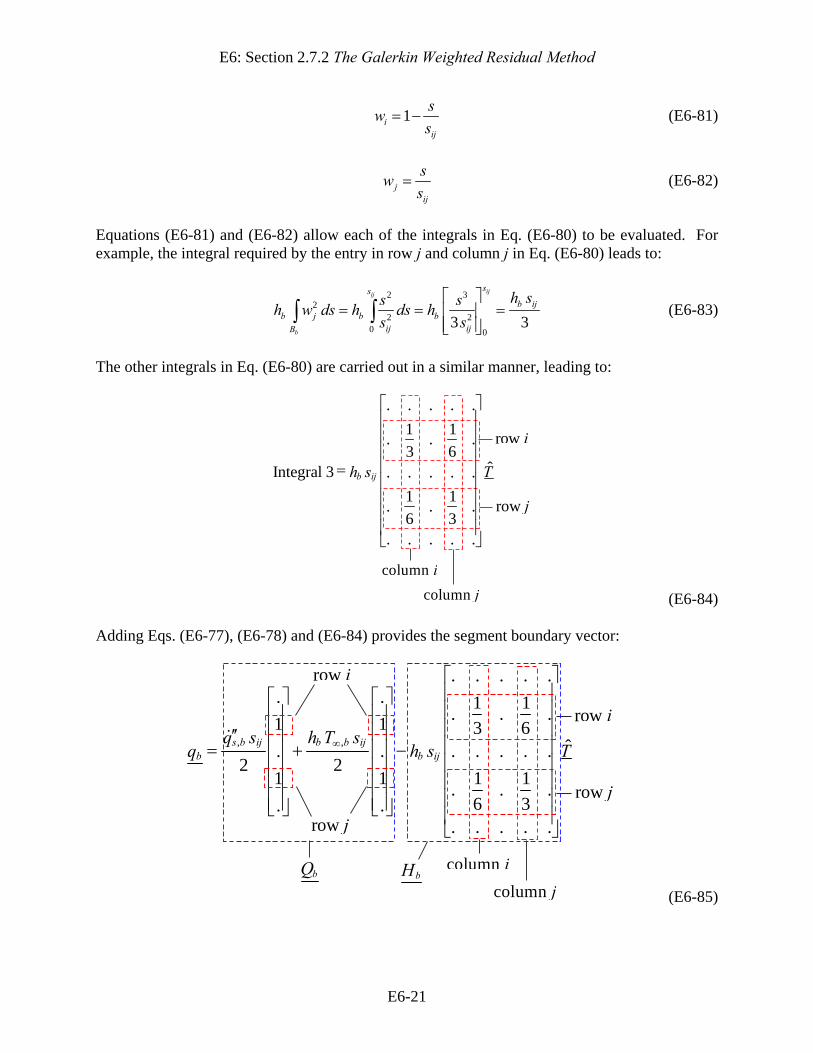
Equations (E6-81) and (E6-82) allow each of the integrals in Eq. (E6-80) to be evaluated. For example, the integral required by the entry in row j and column j in Eq. (E6-80) leads to:

2 3

22 2

0 03 3

ijij

b

ssb ij

b j b bij ijB

h ss sh w ds h ds hs s

⎡ ⎤= = =⎢ ⎥

⎢ ⎥⎣ ⎦∫ ∫ (E6-83)

The other integrals in Eq. (E6-80) are carried out in a similar manner, leading to:

row i

row j

column icolumn j

. . . . .1 1. . .3 6

Întegral 3 . . . . .1 1. . .6 3

. . . . .

b ijh s T

⎡ ⎤⎢ ⎥⎢ ⎥⎢ ⎥⎢ ⎥=⎢ ⎥⎢ ⎥⎢ ⎥⎢ ⎥⎣ ⎦

(E6-84) Adding Eqs. (E6-77), (E6-78) and (E6-84) provides the segment boundary vector:

, ,

. . . . .. . 1 1. . .1 1 3 6

ˆ. . . . . . .2 2

1 1 1 1. . .6 3. .

. . . . .

s b ij b b ijb b ij

q s h T sq h s T∞

⎡ ⎤⎢ ⎥⎡ ⎤ ⎡ ⎤⎢ ⎥⎢ ⎥ ⎢ ⎥⎢ ⎥⎢ ⎥ ⎢ ⎥′′ ⎢ ⎥= + −⎢ ⎥ ⎢ ⎥⎢ ⎥⎢ ⎥ ⎢ ⎥⎢ ⎥⎢ ⎥ ⎢ ⎥⎢ ⎥⎢ ⎥ ⎢ ⎥⎣ ⎦ ⎣ ⎦ ⎢ ⎥⎣ ⎦

row i

row j

column icolumn j

row i

row j

bQ bH (E6-85)


E6-22

Note that the segment boundary vector is composed of a column vector, bQ , and a matrix, bH ,

that multiplies the vector of unknown temperatures. Therefore, the global boundary vector is given by: ˆq Q H T= − (E6-86) where Q and H are assembled from bQ and bH according to:

1

bN

bb

Q Q=

=∑ (E6-87)

and

1

bN

bb

H H=

= ∑ (E6-88)

Substituting Eq. (E6-86) into Eq. (E6-37) leads to the matrix equation that must be solved to obtain the solution to the finite element problem: ˆ ˆK T Q H T= − (E6-89) or ( ) ˆK H T Q+ = (E6-90) Implementing the Solution The finite element problem with linear triangular elements has been reduced to a bookkeeping problem. The information about the problem (e.g., the conductivity and boundary conditions) and the mesh (e.g., the location of the nodal coordinates, elements, and boundary segments) must be used to construct K , H and Q . Once K , H and Q are formed, the matrix equation given

by Eq. (E6-90) is solved to obtain T , the temperature at each node. The process is illustrated in the context of the problem shown in Figure E6-7.


E6-23

2100 W/mq′′ =

2

,

100 W/m -K300 K

t

t

hT∞

==

2

,

50 W/m -K350 K

b

b

hT∞

==

(0,0) (0.25,0)

(0.5,0.25)

(0.5,0.75)(0,0.75)

k = 0.25 W/m-K

Figure E6-7: Two-dimensional conduction problem used to illustrate the finite element solution. The coordinates of points are shown in m. The first step is to define the sub-domains and boundaries that specify the problem. The information about the sub-domains is contained in matrix sd . The number of columns in the matrix sd is equal to the number of sub-domains in the computational domain. The information about each of the sub-domains is contained in the columns. For a more complex problem, the volumetric generation and other parameters might be required. For the simple problem shown in Error! Reference source not found. only the conductivity is required. There is only one sub-domain for the problem, as shown in Figure E6-8, and therefore the matrix sd is setup in the MATLAB script S2p7p2_script according to: clear all; % setup details of computational domain sdm=[0.25]'; % conductivity of each sub-domain The information about the boundary conditions is contained in matrix bc . The number of columns in the matrix bc is equal to the number of boundaries (not boundary elements) in the computational domain. The information about the boundaries is contained in each column: the first row holds the heat transfer coefficient, the second row holds the adjacent fluid temperature, and the third row holds the specified heat flux into the computational domain. There are five boundaries for the problem shown in Figure E6-8 and therefore the matrix bc is setup according to: bcm=[0,0,0; 50,350,0; 0,0,0; 100,300,0; 0,0,100]'; % boundary condition for each boundary which can be examined from the MATLAB command window: >> bcm bcm =


E6-24

0 50 0 100 0 0 350 0 300 0 0 0 0 0 100

2100 W/mq′′ =

2

,

100 W/m -K300 K

t

t

hT∞

==

2

,

50 W/m -K350 K

b

b

hT∞

==

k = 0.25 W/m-K

sub-domain 1

edge 1

edge 4

Figure E6-8: Sub-domains and boundaries that define the problem.

The next step is to define a mesh of triangular elements. A very crude mesh is shown in Figure E6-9.

n1 n2

n3n4n5

n8n7n6

n11 n10 n9

e1e2 e3

e4e5e6

e7

e8e9 e10

e11

b1

b2

b3

b4

b5b6

b7

b8

b9 n = node#e = element #b = boundary segment #

Figure E6-9: A crude mesh. The mesh shown in Figure E6-9 is defined by Nn = 11 nodes. Information about the nodes is stored in the point matrix, p . There are Nn columns in the point matrix. The first row of each

column contains the x-coordinate of the corresponding node and the second row contains the y-coordinate. The point matrix is setup for the grid shown in Figure E6-9 (refer to Figure E6-7 for the dimensions of the problem): % setup details of the grid N_n=11; % number of nodes % setup point matrix - coordinates of each node pm=[0,0; 0.25,0; 0.5,0.25; 0.25,0.25; 0,0.25; 0,0.5; 0.25,0.5; 0.5,0.5; 0.5,0.75; 0.25,0.75; 0,0.75]'; which leads to: >> pm


E6-25

pm = 0 0.2500 0.5000 0.2500 0 0 0.2500 0.5000 0.5000 0.2500 0 0 0 0.2500 0.2500 0.2500 0.5000 0.5000 0.5000 0.7500 0.7500 0.7500 The mesh is defined by Nb = 9 boundary segments. Information about the boundary segments is stored in the edge matrix, e . There are Nb columns in the edge matrix. The first two rows of each column contain the indices of the nodes that define the boundary segment. The third row contains the index of the boundary that the boundary segment lies on (as seen in Figure E6-8). The edge matrix is setup for the mesh shown in Figure E6-9: N_b=9; % number of boundary segments % setup edge matrix - nodes that define each segment and boundary em=[1,2,1; 2,3,2; 3,8,3; 8,9,3; 9,10,4; 10,11,4; 11,6,5; 6,5,5; 5,1,5]'; which leads to: >> em em = 1 2 3 8 9 10 11 6 5 2 3 8 9 10 11 6 5 1 1 2 3 3 4 4 5 5 5 The mesh is defined by Ne = 11 elements. Information about the edge is stored in the triangle matrix, t . There are Ne columns in the triangle matrix. The first three rows contain the indices of the three nodes that define the elements, given in clockwise order. The fourth row contains the number of the sub-domain that the element lies in. The triangle matrix is setup for the mesh shown in Error! Reference source not found.: N_e=11; % number of elements % setup triangle matrix - nodes that define each element and subdomain tm=[5,1,4,1; 1,2,4,1; 4,2,3,1; 4,3,8,1; 7,4,8,1; 6,4,7,1; 6,5,4,1; 11,6,10,1; 6,7,10,1; 10,7,8,1; 10,8,9,1]'; which leads to: >> tm tm = 5 1 4 4 7 6 6 11 6 10 10 1 2 2 3 4 4 5 6 7 7 8 4 4 3 8 8 7 4 10 10 8 9 1 1 1 1 1 1 1 1 1 1 1 The element conduction matrix is derived in Eq. (E6-66), which is repeated below:


E6-26

column i column j column k

row i

row j

row k

( ) ( ) ( )

( ) ( ) ( )

( ) ( ) ( )

2 2

2 22

2 2

. . . . . . .

. . . .

. . . . . . .

. . . .

. . . . . . .

. . . .

. . . . . . .

jk jk jk ik jk ik jk ij jk ij

e ee ik jk ik jk ik ik ik ij ik ijk

ijk

ij jk ij jk ij ik ij ik ij ij

x y x x y y x x y y

A kK x x y y x y x x y yb

x x y y x x y y x y

⎡ ⎤⎢ ⎥

+ − + +⎢ ⎥⎢ ⎥⎢ ⎥⎢ ⎥= − + + − +⎢ ⎥⎢ ⎥⎢ ⎥

+ − + +⎢ ⎥⎢ ⎥⎣ ⎦

(E6-66) The elements associated with the element conduction matrix are added, element by element, to the global conduction matrix according to Eq. (E6-56):

1

eN

ei

K K=

= ∑ (E6-91)

The global conduction matrix is initialized: K=zeros(N_n,N_n); % global conduction matrix initialization The global conduction matrix is constructed element-by-element within a for loop: for e=1:N_e The indices of the three nodes that define the element and the subdomain that the element belongs to are obtained from the triangle matrix: i=tm(1,e); % index of node i j=tm(2,e); % index of node j k=tm(3,e); % index of node k d=tm(4,e); % subdomain of element The x- and y-distances separating the nodes (xij, xik, etc.) are computed using Eqs. (E6-40) through (E6-45); the coordinates of the nodes are obtained from the point matrix: xij=pm(1,j)-pm(1,i); % x-distance between nodes j and i in element e xik=pm(1,k)-pm(1,i); % x-distance between nodes k and i in element e xjk=pm(1,k)-pm(1,j); % x-distance between nodes k and j in element e yij=pm(2,j)-pm(2,i); % y-distance between nodes j and i in element e yik=pm(2,k)-pm(2,i); % y-distance between nodes k and i in element e yjk=pm(2,k)-pm(2,j); % y-distance between nodes k and j in element e


E6-27

The parameter bijk and the area of the element are computed using Eqs. (E6-47) and (E6-46), respectively: bijk=xij*yjk-xjk*yij; Ae=abs(bijk)/2; % area of element e The conductivity of the element is obtained from the matrix sd and the elements of the element conduction matrix are added to the global conduction matrix according to Eq. (E6-66). % add element conduction matrix to global conduction matrix ke=sdm(1,d); % conductivity of element K(i,i)=K(i,i)+Ae*ke*(xjk^2+yjk^2)/bijk^2; K(i,j)=K(i,j)-Ae*ke*(xjk*xik+yjk*yik)/bijk^2; K(i,k)=K(i,k)+Ae*ke*(xjk*xij+yjk*yij)/bijk^2; K(j,i)=K(j,i)-Ae*ke*(xik*xjk+yik*yjk)/bijk^2; K(j,j)=K(j,j)+Ae*ke*(xik^2+yik^2)/bijk^2; K(j,k)=K(j,k)-Ae*ke*(xik*xij+yik*yij)/bijk^2; K(k,i)=K(k,i)+Ae*ke*(xij*xjk+yij*yjk)/bijk^2; K(k,j)=K(k,j)-Ae*ke*(xij*xik+yij*yik)/bijk^2; K(k,k)=K(k,k)+Ae*ke*(xij^2+yij^2)/bijk^2; end The vector bQ and matrix bH are derived in Eq. (E6-85), which is repeated below:

, ,

. . . . .. . 1 1. . .1 1 3 6

ˆ. . . . . . .2 2

1 1 1 1. . .6 3. .

. . . . .

s b ij b b ijb b ij

q s h T sq h s T∞

⎡ ⎤⎢ ⎥⎡ ⎤ ⎡ ⎤⎢ ⎥⎢ ⎥ ⎢ ⎥⎢ ⎥⎢ ⎥ ⎢ ⎥′′ ⎢ ⎥= + −⎢ ⎥ ⎢ ⎥⎢ ⎥⎢ ⎥ ⎢ ⎥⎢ ⎥⎢ ⎥ ⎢ ⎥⎢ ⎥⎢ ⎥ ⎢ ⎥⎣ ⎦ ⎣ ⎦ ⎢ ⎥⎣ ⎦

row i

row j

column icolumn j

row i

row j

bQ bH (E6-84)

These variables are initialized: Q=zeros(N_n,1); % global boundary vector initialization H=zeros(N_n,N_n); % global convection matrix initialization and constructed boundary segment-by-boundary segment using a for loop: for b=1:N_b


E6-28

The indices of the two nodes that define the boundary segment and the boundary that the segment belongs to are obtained from the edge matrix: i=em(1,b); % index of node i j=em(2,b); % index of node j bndry=em(3,b); % boundary of boundary segment The x- and y-distance separating the nodes and the linear distance between the nodes, sij, are computed: xij=pm(1,j)-pm(1,i); % x-distance between nodes j and i on boundary segment b yij=pm(2,j)-pm(2,i); % y-distance between nodes j and i on boundary segment b sij=sqrt(xij^2+yij^2); % length of boundary segment b The specified heat flux, heat transfer coefficient, and ambient temperature associated with the boundary segment is obtained from the matrix bc and the elements of bQ and bH are added to

the global vector Q and matrix H according to Eq. (E6-85). qfsb=bcm(3,bndry); % specified heat flux (W/m^2) hb=bcm(1,bndry); % heat transfer coefficient (W/m^2-K) Tinfb=bcm(2,bndry); % ambient temperature (K) % add segment boundary vector to global boundary vector Q(i,1)=Q(i,1)+qfsb*sij/2+hb*Tinfb*sij/2; Q(j,1)=Q(j,1)+qfsb*sij/2+hb*Tinfb*sij/2; % add segment convection matrix to global convective matrix H(i,i)=H(i,i)+hb*sij/3; H(i,j)=H(i,j)+hb*sij/6; H(j,i)=H(j,i)+hb*sij/6; H(j,j)=H(j,j)+hb*sij/3; end The temperatures at each node are obtained from Eq. (E6-90): T=(K+H)\Q; % obtain temperatures at each node which leads to: >> T T = 456.9587 353.6660 349.3872 381.2069 460.2514 421.6331 361.5230 343.2677


E6-29

300.6376 299.9842 303.2351 The organization of the mesh information is nearly the same as is used by the PDE toolbox in MATLAB. Therefore, the tools and commands that are available in the PDE toolbox can be used to manipulate and investigate this solution. If your version of MATLAB includes the PDE toolbox, then the solution can be plotted using the pdeplot command: pdeplot(pm,em,tm,'xydata',T,'contour','on'); which leads to Figure E6-10.

Figure E6-10: Contour plot of the finite element solution.

The PDE toolbox has a graphical user interface that can be used to quickly setup a computational domain and generate a mesh. From the command window, type: >> pdetool to open the graphical user interface. Specify the computational domain shown in Figure E6-7 using the polygon tool. Set the application to Heat Transfer from the Options menu. Select Initialize Mesh and Refine Mesh from the Mesh menu (Figure E6-11).


E6-30

Figure E6-11: Mesh generated by the PDE toolbox.

Select Export Mesh from the Mesh menu and the point matrix, edge matrix, and triangle matrix associated with the mesh generated by the PDE toolbox are exported to the command space. The refined mesh can be used in place of the coarse mesh that was generated manually by commenting out the specified values of p , e , and t . %clear all; % setup details of computational domain sdm=[0.25]'; % conductivity of each sub-domain bcm=[0,0,0; 50,350,0; 0,0,0; 100,300,0; 0,0,100]'; % boundary condition for each boundary % % setup details of the grid % N_n=11; % number of nodes % % setup point matrix - coordinates of each node % pm=[0,0; 0.25,0; 0.5,0.25; 0.25,0.25; 0,0.25; 0,0.5; 0.25,0.5; 0.5,0.5; 0.5,0.75; 0.25,0.75; 0,0.75]'; % % N_b=9; % number of boundary segments % % setup edge matrix - nodes that define each segment and boundary % em=[1,2,1; 2,3,2; 3,8,3; 8,9,3; 9,10,4; 10,11,4; 11,6,5; 6,5,5; 5,1,5]'; % % N_e=11; % number of elements % % setup triangle matrix - nodes that define each element and subdomain % tm=[5,1,4,1; 1,2,4,1; 4,2,3,1; 4,3,8,1; 7,4,8,1; 6,4,7,1; 6,5,4,1,; 11,6,10,1; 6,7,10,1; 10,7,8,1; 10,8,9,1]';


E6-31

The structure of the point matrix and triangle matrix is identical to the ones that were generated manually: [g,N_n]=size(p); % number of nodes pm=p; % point matrix is equal to the one produced by pdetool [g,N_e]=size(t); % number of elements tm=t; % triangle matrix is equal to the one produced by pdetool The first two rows of the edge matrix generated by MATLAB's PDE toolbox are identical to ours. The index of the boundary is contained in row five of the edge matrix generated by the PDE toolbox: [g,N_b]=size(e); % number of boundary segments em=zeros(3,N_b); % initialize edge matrix em(1,:)=e(1,:); % index of node i em(2,:)=e(2,:); % index of node j em(3,:)=e(5,:); % boundary Otherwise, the script S2p7p2_script remains unchanged. The solution generated with the more refined mesh is shown in Figure E6-12.

Figure E6-12: Contour plot of the finite element solution with the refined mesh generated by the PDE toolbox.

Documents

Section 2.7.2 Galerkin Method