Second Young Researchers Workshop · Second Young Researchers Workshop ... Daniel Hernandez The Flavour of Seesaw ... Estimate of the GUT-favoured region for the universal case, X

Second Young Researchers Workshop “Physics Challenges in the LHC Era”

2010

II

FRASCATI PHYSICS SERIES Series Editor Danilo Babusci Technical Editor Luigina Invidia Cover by Claudio Federici

Volume LI

Istituto Nazionale di Fisica Nucleare – Laboratori Nazionali di Frascati Divisione Ricerca SIDS – Servizio Informazione e Documentazione Scientifica Ufficio Biblioteca e Pubblicazioni P.O. Box 13, I–00044 Frascati Roma Italy email: [email protected]

III

IV

FRASCATI PHYSICS SERIES Second Young Researchers Workshop “Physics Challenges in the LHC Era” 2010 Copyright © 2010 by INFN All rights reserved. No part of this publication may be reproduced, stored in a retrieval system or transmitted, in any form or by any means, electronic, mechanical, photocopying, recording or otherwise, without the prior permission of the copyright owner. IS BN 978–88–86409–60–5

V

FRASCATI PHYSICS SERIES

Volume LI

Second Young Researchers Workshop “Physics Challenges in the LHC Era”

2010

Editor Enrico Nardi

Frascati, May 10th and May 13th, 2010

VI

International Advisory Committee G. Altarelli Università Roma Tre W. Buchmuller DESY F. Ceradini Università Roma Tre A. Di Ciaccio Università Roma Tor Vergata J. Ellis CERN B. Grinstein University of California San Diego R. Fiore Università della Calabria Local Organizing Committee M. Antonelli INFN Frascati, D. Aristizabal INFN Frascati & Université de Liège O. Cata INFN Frascati V. Del Duca INFN Frascati R. Faccini Università Roma La Sapienza & INFN Roma G. Isidori INFN Frascati J. F. Kamenik INFN Frascati & JSI E. Nardi INFN Frascati (School Director) M. Palutan INFN Frascati T. Spadaro INFN Frascati

VII

PREFACE

The second Young Researcher Workshop “Physics Challenges in the LHC Era” was held in the Frascati Laboratories during May 10th and 13th 2010, in conjunction with the 15th edition of the Frascati Spring School ”Bruno Touschek”.

The Frascati Young Researcher Workshop provides an opportunity for the students attending the Spring School to complement the scientific program by giving short lectures to their colleagues on their specific research topics. The Workshop also constitutes an important step in the scientific formation of our students: they learn how to organize a presentation on a specialistic subject that should be understandable for a general audience of young physicists in the training stage, and how to condense the results of their work within a fifteen minutes talk. They get a training in preparing a write up of their speech for the Workshop Proceedings, and they also experience how to interact with the Scientific Editor and with the Editorial Office of the Frascati Physics Series. Eventually, they also learn how to prepare a submission of their preprint to the arXive database. Helping to develop these skills is an integral part of the scientific formation the Frascati Spring School is aiming to.

The second edition of the Young Researcher Workshop confirmed the success of the first edition. We received a number of applications larger than what could be allotted within the two afternoons of the Workshop, and regrettedly we could not satisfy all the requests to give a talk. The resulting scientific program of the workshop was rich and quite interesting, covering a large variety of actual topics both in theoretical and experimental particle physics.

These proceedings, that collect the joint efforts of the speakers of the Young Researchers Workshop, testify the remarkably high professional level of all the contributions, and give a benchmark for the scientific level required to participate in future editions of the Workshop. They can also provide useful guidelines for structuring the presentations of our future young lecturers.

Too many people contributed to the success of the Young Researcher Workshop "Physics Challenges in the LHC Era" and of the joint XV Frascati Spring

VIII

School "Bruno Touschek" to give here a complete list. However, a special acknowledgment must be given to the Workshop secretariat staff and backbones of the Frascati Spring School Maddalena Legramante, Silvia Colasanti and Angela Mantella. To Claudio Federici, that put a special effort in realizing the graphics of the Workshop and School posters, to Luigina Invidia for the technical editing of these proceedings, and to the Director of the Frascati Laboratories Mario Calvetti for his support. Frascati, July 2010 Enrico Nardi

IX

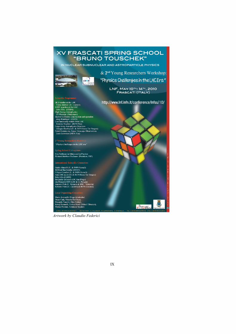
Artwork by Claudio Federici

X

XI

CONTENTS

Preface ............................................................................................ VII Ennio Salvioni Minimal Z' Models and the Early LHC ..............................1 Jure Drobnak Model Independent Analysis of FCNC Top Quark Decays ........................................................................ 7 Roberto Barceló Higgs Bosons in

!

tt Production ..................................... 13 Paolo Lodone Increasing the Lightest Higgs Mass Bound of the MSSM .......................................................................19 Maria Ilaria Besana Study of W+Jets Background to Top Quark Pair Production Cross Section in ATLAS at the LHC ......... 25 Roberto Iuppa Monitoring The Mrk421 Flaring Activity by the ARGO-YBJ Experiment .....................................................31 Izabela Balwierz Study of the Decoherence of Entangled Kaons by the Interaction with Thermal Photons .....................................37 Tomasz Twaróg Investigations of the Time Interval Distributions between the Decays of Quantum Entangled Neutral Kaons................................................................................... 43 Rodrigo A. De Pablo MINSIS & Minimal Flavour Violation .......................... 49 Daniel Hernandez The Flavour of Seesaw ..................................................... 55 Jackson M. S. Wu Natural Dirac Neutrinos from Warped Extra Dimension ......................................................................... 61 Chee Sheng Fong Flavour in Soft Leptogenesis............................................. 67 Pablo Villanuevra-Pérez Model Independent and Genuine First Observation of Time Reversal Violation ...............................................73 Marc Ramon Measuring sin φS From New Physics Polluted B Decays...............................................................................79

Frascati Physics Series Vol. LI (2010), pp. 1-62nd Young Researchers Workshop: Physics Challenges in the LHC Era

Frascati, May 10 and 13, 2010

MINIMAL Z ′ MODELS AND THE EARLY LHC

Ennio SalvioniDipartimento di Fisica, Universita di Padova and INFN, Sezione di Padova

Via Marzolo 8, I-35131 Padova, Italy

Abstract

We consider a class of minimal extensions of the Standard Model with an extramassive neutral gauge boson Z ′. They include both family-universal models,where the extra U(1) is associated with (B − L), and non-universal modelswhere the Z ′ is coupled to a non-trivial linear combination of B and the leptonflavours. After giving an estimate of the range of parameters compatible with aGrand Unified Theory, we present the current experimental bounds, discussingthe interplay between electroweak precision tests and direct searches at theTevatron. Finally, we assess the discovery potential of the early LHC.

1 Introduction

Extra neutral gauge bosons, known in the literature as Z ′, appear in many

proposals for Beyond-the-Standard Model (BSM) physics; for a review, see for

1

instance 1). Here we focus on minimal Z ′, previously studied in 2), which

stand out both for their simplicity, and because they could arise in several

of the above mentioned BSM scenarios, such as, e.g., Grand Unified Theories

(GUTs) and string compactifications.

2 Theory

Following 3), we consider a minimal extension of the SM gauge group that

includes an additional Abelian factor, labeled U(1)X , commuting with SU(3)c×

SU(2)L × U(1)Y . The fermion content of the SM is augmented by one right-

handed neutrino per family. We require anomaly cancellation, as this allows us

to write a renormalizable Lagrangian. If family-universality is imposed, then

the anomaly cancellation conditions yield a unique solution: X = (B − L),

where B and L are baryon and lepton number respectively 1. However, if the

requirement of family-universality is relaxed, it can be shown that the following

set of family-dependent charges satisfy the anomaly cancellation conditions:

X =∑

a=e, µ, τ (λa/3)(B − 3La) , where La are the lepton flavours, and λa are

arbitrary coefficients. We will consider a specific example of such non-universal

Z ′ in the following.

In the basis of mass eigenstates for vectors, and with canonical kinetic

terms, the neutral current Lagrangian reads

LNC = eJµemAµ + gZ

(ZµJµ

Z + Z ′

µJµZ′

), (1)

where Aµ is the photon field coupled to the electromagnetic current, while

(Zµ, Z ′

µ) are the massive states, which couple to the currents (JµZ , Jµ

Z′) respec-

tively, obtained from Jµ

Z0 =∑

f

[T3L(f) − sin2 θW Q(f)

]fγµf and Jµ

Z′ 0 =∑f [gY Y (f) + gX X(f)] fγµf via a rotation of the Z−Z ′ mixing angle θ′. The

explicit expression of the latter reads tan θ′ = −(gY /gZ)M2Z0/(M2

Z′ − M2Z0) .

Thus, under our minimal assumptions, only three parameters beyond the SM

ones are sufficient to describe the Z ′ phenomenology: the physical mass of the

extra vector, MZ′ , and the two coupling constants (gY , gX). In the follow-

ing discussion, we normalize these couplings to the SM Z0 coupling, namely

gY,X = gY,X/gZ .

1The most general solution to the anomaly cancellation conditions is X =a Y + b (B − L), with a, b arbitrary coefficients. However, the Y componentcan be absorbed in the kinetic mixing in the class of models we consider.

2

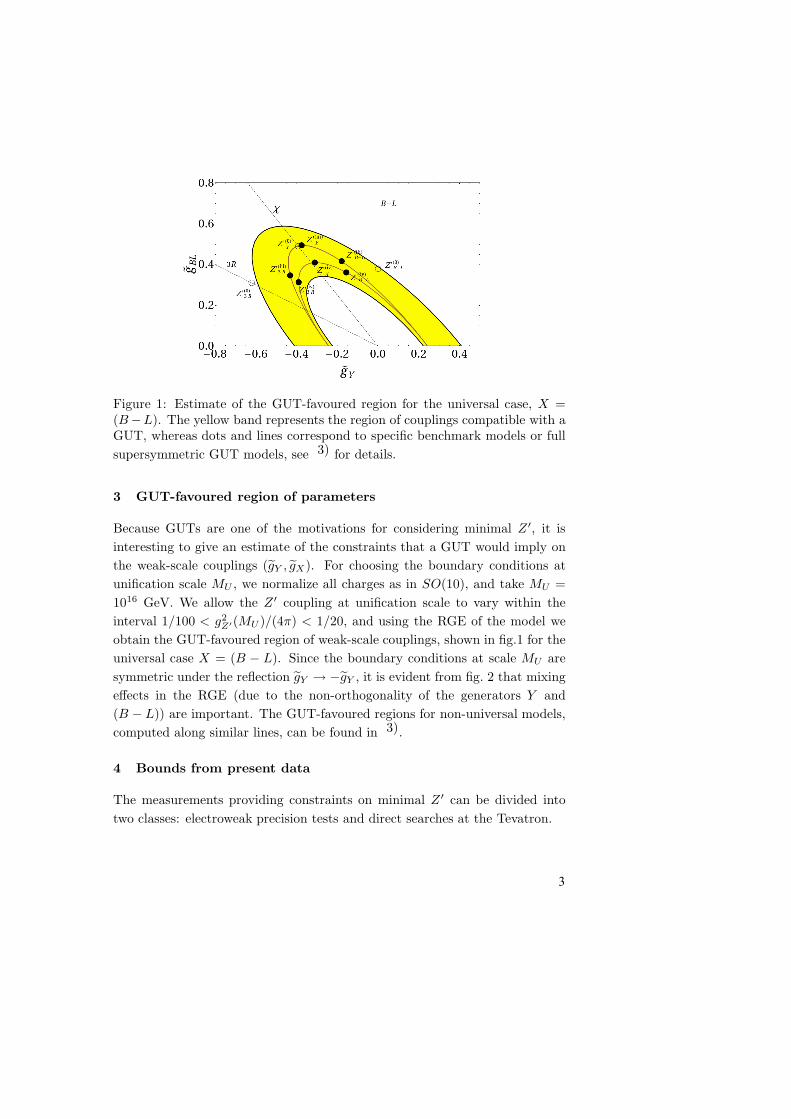
Figure 1: Estimate of the GUT-favoured region for the universal case, X =(B−L). The yellow band represents the region of couplings compatible with aGUT, whereas dots and lines correspond to specific benchmark models or full

supersymmetric GUT models, see 3) for details.

3 GUT-favoured region of parameters

Because GUTs are one of the motivations for considering minimal Z ′, it is

interesting to give an estimate of the constraints that a GUT would imply on

the weak-scale couplings (gY , gX). For choosing the boundary conditions at

unification scale MU , we normalize all charges as in SO(10), and take MU =

1016 GeV. We allow the Z ′ coupling at unification scale to vary within the

interval 1/100 < g2Z′(MU )/(4π) < 1/20, and using the RGE of the model we

obtain the GUT-favoured region of weak-scale couplings, shown in fig.1 for the

universal case X = (B − L). Since the boundary conditions at scale MU are

symmetric under the reflection gY → −gY , it is evident from fig. 2 that mixing

effects in the RGE (due to the non-orthogonality of the generators Y and

(B − L)) are important. The GUT-favoured regions for non-universal models,

computed along similar lines, can be found in 3).

4 Bounds from present data

The measurements providing constraints on minimal Z ′ can be divided into

two classes: electroweak precision tests and direct searches at the Tevatron.

3

4.1 Electroweak precision tests

Measurements performed at LEP1 and at low energy mainly constrain Z − Z ′

mixing, whereas data collected at LEP2 (above the Z pole) constrain effective

four-fermion operators. To compute the bounds from EWPT on minimal Z ′, we

integrate out the heavy vector and use the effective Lagrangian thus obtained

to perform a global fit to the data. The results are shown in fig. 1, for the

universal ‘χ model’, corresponding to a particular direction in the (gY , gX)

plane often considered in the literature.

4.2 Tevatron direct searches

The CDF and D0 collaborations have derived, from the non-observation of

discrepancies with the SM expectations, upper limits on σ(pp → Z ′)×Br(Z ′ →

ℓ+ℓ−) (ℓ = e, µ), 4). To extract bounds on minimal Z ′, we compute the same

quantity at NLO in QCD, and compare it with the limits published by the

experimental collaborations. The comparison between bounds from EWPT

and from the Tevatron is most clear if we plot them in (coupling vs. mass),

for a chosen direction in the (gY , gBL) plane, as it is done in fig. 2 for the

χ model. We see that bounds from EWPT have a linear behaviour, because

all the effects due to the Z ′ in the low-energy effective Lagrangian depend on

the ratio gZ′/MZ′ , whereas bounds from the Tevatron become negligible above

a kinematic limit, which is of the order of 1 TeV. Thus for low masses the

Tevatron data give the strongest limits, while above a certain value of MZ′

(which is of the order of 500 GeV for the χ model), bounds from EWPT are

stronger. In particular, for models compatible with GUTs the strongest bounds

are those given by EWPT.

5 Early LHC reach

The present schedule foresees that in 2010/2011 the LHC will run at 7 TeV in

the center of mass, collecting up to 1 fb−1 of integrated luminosity L. Therefore,

it is interesting to ask whether there are any minimal Z ′ which are both allowed

by present constraints and accessible for discovery in such early phase. To

answer this question, we have performed a NLO analysis similar to the one

used in extracting bounds from Tevatron data, requiring the Z ′ signal to be

at least a 5σ fluctuation over the SM-Drell Yan background. The results are

4

Figure 2: (left) Comparison of bounds from EWPT (red), Tevatron (blue), anddiscovery reach of the early LHC (green curves, from left to right: 50, 100, 200,400 and 1000 pb−1 at 7 TeV, and 400 pb−1 at 10 TeV) for the χ model. (right)Present bounds and discovery prospects of the LHC at 7 TeV and 50 pb−1 forthe muonphilic model with gY = 0. For gX > 0.3 , both the bounds from theTevatron and the LHC reach are indeed weaker, because of finite-width effectsnot included in the figure, but the general message is unaffected. The yellowbands correspond to the GUT-favored region, see Section 3.

displayed for the χ model in fig. 2, where a comparison with present bounds is

made. We see that for L ∼ 100 pb−1 (the luminosity approximately foreseen

at the end of 2010), no discovery is possible. On the other hand, for L ∼ 1 fb−1

some unexplored regions become accessible; however, Z ′ compatible with GUTs

are still out of reach, and more energy and luminosity will be needed to test

them.

5.1 The muonphilic model

We have seen that universal models are strongly constrained by present data.

On the other hand, when we consider non-universal couplings to leptons, the

bounds can be significantly altered. In particular, let us consider the case where

X = B − 3Lµ, which we called ‘muonphilic Z ′ ’. Let us further assume that

kinetic mixing is negligible, i.e. gY ≈ 0. In this case, the Z ′ has no coupling

to the first and third leptonic families, in particular it has no coupling to the

electron. As a consequence, bounds from EWPT are strongly relaxed, the only

surviving constraints coming from (g − 2)µ and ν-N scattering (NuTeV). On

the other hand, the Tevatron reach is limited, as already noted in Section 4,

to MZ′ ≤ 1 TeV: therefore the LHC has access to a wide region of unexplored

5

parameter space already with a very low integrated luminosity at 7 TeV, as

shown in fig. 2.

6 Summary

We have discussed the present experimental bounds and the early LHC reach

on minimal Z ′ models, showing that present constraints cannot be neglected

when assessing the discovery potential of the early LHC. In particular, we have

found that exploration of universal models, coupled to (B − L), may need

more energy and luminosity than those foreseen for 2010/2011, in particular

for values of the couplings compatible with GUTs. On the other hand, some

non-universal models which are weakly constrained by present data, such as

the muonphilic Z ′, could be discovered at the LHC with very low integrated

luminosity.

7 Acknowledgements

I am indebted to my collaborators F. Zwirner, G. Villadoro, and A. Strumia. I

would also like to thank the organizers of the 2nd Young Researchers Workshop

Physics Challenges in the LHC Era for giving me the possibility to present this

work.

References

1. P. Langacker, Rev. Mod. Phys. 81 (2008) 1199, arXiv:0801.1345 [hep-ph].

2. T. Appelquist, B. A. Dobrescu and A. R. Hopper, Phys. Rev. D 68 (2003)

035012, arXiv:hep-ph/0212073.

3. E. Salvioni, G. Villadoro and F. Zwirner, JHEP 0911 (2009) 068,

arXiv:0909.1320 [hep-ph]; E. Salvioni, A. Strumia, G. Villadoro and

F. Zwirner, JHEP 1003 (2010) 010, arXiv:0911.1450 [hep-ph].

4. T. Aaltonen et al. [CDF Collaboration], Phys. Rev. Lett. 102 (2009)

031801, arXiv:0810.2059 [hep-ex]; T. Aaltonen et al. [CDF Collabo-

ration], Phys. Rev. Lett. 102 (2009) 091805, arXiv:0811.0053 [hep-

ex]; [D0 collaboration], D0 note 5923-CONF (July 2009), http://www-

d0.fnal.gov/Run2Physics/WWW/results/np.htm.

6



MODEL INDEPENDENT ANALYSIS OF FCNC

TOP QUARK DECAYS

Jure DrobnakJozef Stefan Institute, Jamova cesta 39, 1000 Ljubljana, Slovenia

Svjetlana Fajfer and Jernej F. KamenikJozef Stefan Institute, Jamova cesta 39, 1000 Ljubljana, Slovenia

Abstract

We study flavor changing neutral current decays of the top quark, t → cZ andt → cγ. These decays are highly suppressed in the standard model. Numerousextensions of the standard model however, still allow significant enhancementof the branching ratios for such processes. Using model independent effectiveLagrangian approach, we perform a full next-to-leading order QCD analysisand the impact it may have on the observability of such FCNC processes. Wealso study t → cℓ+ℓ− decays and observables that could help to discriminateamong variety of new physics scenarios.

1 Introduction

The standard model (SM) predicts highly suppressed flavour changing neutral

current (FCNC) processes of the top quark (t → cV, V = Z, γ, g) while new

7

physics beyond the SM (NP) in many cases lifts this suppression (for a recent

review c.f. 1)).

Top quark FCNCs can be probed both in production and in decays.

Present experimental upper bounds on branching ratios are at a precent

level 2, 3, 4). The LHC will be producing about 80, 000 tt events per day

at the luminosity L = 1033cm−2s−1 and will be able to access rare top decay

branching ratios at the 10−5 level with 10fb−1 5).

We present two of our recent works in treating FCNC top quark decay in a

model independent way. First 6) is dedicated to the two-body final state decays,

where we perform a full next-to-leading order (NLO) QCD analysis. We study

operator renormalization effects as well as finite matrix element corrections.

The second 7) is dedicated to the three-body final state decays t → cℓ+ℓ− where

the Z boson or the virtual photon emerging from the FCNC vertex is considered

to further decay into a lepton pair. Exploring this decay channel offers the

advantage to consider more observables – in particular angular asymmetries

among the final lepton and jet directions. Our goal is to discriminate different

types of FCNC couplings.

2 Effective Lagrangian

In writing the effective top FCNC Lagrangian we follow roughly the notation

of ref. 1, 8). Hermitian conjugate and chirality flipped operators are implicitly

contained in the Lagrangian

Ltceff =

v

Λ2

∑

V =g,γ,Z

bVLRO

VLR +

v2

Λ2aZ

LOZL + (L ↔ R) + h.c. , (1)

where OVLR,RL = gV V a

µν qL,RT aσµνtR,L, OZL,R = gZZµqL,RγµtL,R, q = c(u),

qR,L = (1 ± γ5)q/2, σµν = i[γµ, γν ]/2, gZ = 2e/ sin 2θW , gγ = e, gg =√

αs4π.

Furthermore V (A, Z)µν = ∂µVν − ∂νVµ, Gaµν = ∂µGa

ν − ∂νGaµ + gfabcG

bµGc

ν ,

and T a are the Gell-Mann matrices in the case of the gluon and 1 for the γ, Z.

Finally v = 246 GeV is the electroweak condensate and Λ is the effective scale

of NP. The lepton couplings to the Z, γ bosons in the t → cℓ+ℓ− analysis are

considered to be SM-like.

8

3 NLO QCD corrections to t → cZ, γ

3.1 Renormalization effects

QCD virtual corrections to effective operators in eq.(1) involve ultra violet

(UV) divergencies. These are cancelled exactly in the matching procedure

to the underlying NP theory. The remaining logarithmic dependence on the

matching scale can be resumed using renormalization group (RG) methods.

The effective couplings are evolved from the high scale Λ down to the top

quark mass scale µt.

We investigate the values of bγ,Z1 at the top mass scale µt ≃ 200 GeV

induced solely by the mixing of the gluonic dipole contribution produced at the

UV scale Λ. We find that for Λ above 2 TeV these contributions are around

10% of bg(Λ) for bγ , but much smaller (below 1 %) for bZ .

3.2 Matrix element corrections

To consistently describe rare top decays at NLO in αs one has to take into

account finite QCD loop corrections evaluated at the top mass scale as well as

single gluon bremsstrahlung corrections, which cancel the associated infrared

divergencies in the decay rates. In ref. 9) we give these results in a complete

analytical form. In the case of the photon we also investigate the influence of

the experimentally motivated kinematical cuts on the photon energy Ecutγ and

the angle between the photon and the c-jet δr = 1−pγ ·pj/EγEj . We analyze

the change of decay rates and branching ratios when going from leading order

(LO) to NLO in QCD, where branching ratio for the top quark is defined as

Br(t → cZ, γ) = Γ(t → cZ, γ)/Γ(t → bW ). The results for the Z case are

summarized in tab.1. The change in the decay width is of the order 10%.

Due to the cancellation of NLO corrections to t → cZ decay rates and the

main decay channel rate, the change in branching ratios are only at a promile

level for bg = 0. However, setting bg to be equal to aZ or bZ , the change is

increased by an order of magnitude and reaches a few percent. The results for

the photon case are summarized by fig.1. We observe a significant dependence

of the relative change of Br on the kinematical cuts. It can reach 10 − 15%

1Chirality assignments are implicit so bi stands for biLR or bi

RL, for i =Z, γ, g.

9

Table 1: Ratios between NLO and LO decay rates and branching ratios given

for certain values and relations between FCNC coefficients for t → cZ. SM

inputs used are: mt = 172.3 GeV, mZ = 91.2 GeV, sin2 θW = 0.231.

bZ = 0 aZ = 0 aZ = bZ bZ = 0 aZ = 0bg = 0 bg = 0 bg = 0 aZ = bg bZ = bg

ΓNLO/ΓLO 0.92 0.91 0.92 0.95 0.94

BrNLO/BrLO 1.001 0.999 1.003 1.032 1.022

Figure 1: Relative size of αs corrections to the Br(t → cγ) at representative

ranges of δr and Ecutγ . Contours of constant correction values are plotted for

bg = 0 (gray, dotted), bg = bγ (red) and bg = −bγ (blue, dashed).

when bg ∼ bγ . Consequently, a bound on Br(t → cγ) can, depending on the

experimental cuts, probe both bg,γ couplings.

4 Angular asymmetries in t → cℓ+ℓ−

We define two angles θj and θl. The first one is defined in the ℓ+ℓ− rest-frame

zj = cos θj and measures the relative direction between the positively charged

lepton and the light quark jet. Conversely, in the rest-frame of the positive

lepton and the quark jet, we can define zℓ = cos θℓ to measure the relative

directions between the two leptons. In terms of these variables, we can define

two asymmetries (i = j, ℓ) as

Ai =Γzi>0 − Γzi<0

Γzi>0 + Γzi<0

, (2)

10

where we have denoted Γzi<0, Γzi>0 as the integrated decay rates with an upper

or lower cut on one of the zi variables. We can then identify Aj ≡ AFB as the

commonly known forward-backward asymmetry and define Al ≡ ALR as the

left-right asymmetry.

In 7) we present analytical formulae for the two asymmetries and explore

the possible ranges and correlations between the two asymmetries. Fixing the

total decay rate we scan over the FCNC coupling parameter space plotting

points in (AFB, ALR) plane. Two such plots are shown in fig.2.

-0,15 -0,10 -0,05 0,00 0,05 0,10 0,150,00

0,05

0,10

0,15

0,20

0,25

0,30

0,35

All couplings aZ

L = 0

bZLR = bZ

RL = 0

aZL = aZ

R = 0

ALR

AFB

-0,15 -0,10 -0,05 0,00 0,05 0,10 0,150,00

0,06

0,12

0,18

0,24

0,30

0,36

0,42

0,48 Photon and Z Z only bZ

LR = bZRL = 0

A

LR

AFB

Figure 2: Left: The correlation of AFB and ALR in Z mediated transition.

Right: The correlation of AFB and ALR in Z and γ mediated transition.

We see that AFB cannot exceed ∼ 10 % even when the interference of

t → cZ and t → cγ is considered. This interference can, however, increase ALR

by more then 10 %.

5 Conclusions

We have found that especially in the t → cγ decay we can expect the effects of

NLO QCD corrections to be significant. Furthermore effects of the kinematical

cuts of the nontrivial photon spectrum should be taken into account. We

have found two angular asymmetries that can be used in t → cℓ+ℓ− decay to

discriminate between different couplings governing the FCNC decay.

11

References

1. J. A. Aguilar-Saavedra, Acta Phys. Polon. B 35, 2695 (2004) [arXiv:hep-

ph/0409342].

2. T. Aaltonen et al. [CDF Collaboration], Phys. Rev. Lett. 101, 192002

(2008) [arXiv:0805.2109 [hep-ex]].

3. S. Chekanov et al. [ZEUS Collaboration], Phys. Lett. B 559, 153 (2003)

[arXiv:hep-ex/0302010].

4. T. Aaltonen et al. [CDF Collaboration], Phys. Rev. Lett. 102 (2009) 151801

[arXiv:0812.3400 [hep-ex]].

5. J. Carvalho et al. [ATLAS Collaboration], Eur. Phys. J. C 52, 999 (2007)

[arXiv:0712.1127 [hep-ex]].

6. J. Drobnak, S. Fajfer and J. F. Kamenik, arXiv:1004.0620 [hep-ph].

7. J. Drobnak, S. Fajfer and J. F. Kamenik, JHEP 0903 (2009) 077

[arXiv:0812.0294 [hep-ph]].

8. J. A. Aguilar-Saavedra, Nucl. Phys. B 812, 181 (2009) [arXiv:0811.3842

[hep-ph]].

9. J. Drobnak, S. Fajfer and J. F. Kamenik, in preparation.

12



HIGGS BOSONS IN tt PRODUCTION

Roberto BarceloCAFPE and Departamento de Fısica Teorica y del Cosmos,

Universidad de Granada, E-18071 Granada, Spain.

Abstract

The top quark has a large Yukawa coupling with the Higgs boson. In theusual extensions of the standard model the Higgs sector includes extra scalars,which also tend to couple strongly with the top quark. Unlike the Higgs,these fields have a natural mass above 2mt, so they could introduce anomaliesin tt production at the LHC. We study their effect on the tt invariant massdistribution at

√s = 7 TeV. We focus on the bosons (H ,A) of the minimal

SUSY model and on the scalar field (r) associated to the new scale f in LittleHiggs (LH) models. We show that in all cases the interference with the standardamplitude dominates over the narrow-width contribution. As a consequence,the mass difference between H and A or the contribution of an extra T -quarkloop in LH models become important effects in order to determine if these fieldsare observable there. We find that a 1 fb−1 luminosity could probe the regiontanβ ≤ 3 of SUSY and v/(

√2f) ≥ 0.3 in LH models.

13

1 Introduction

The main objective of the LHC is to reveal the nature of the mechanism break-

ing the electroweak symmetry. This requires not only a determination of the

Higgs mass and couplings, but also a search for additional particles that may

be related to new dynamics or symmetries present at the TeV scale. The top-

quark sector appears then as a promising place to start the search, as it is there

where the EW symmetry is broken the most. Generically, the large top-quark

Yukawa coupling with the Higgs boson (h) also implies large couplings with

the extra physics. For example, in SUSY extensions h comes together with

neutral scalar (H) and pseudoscalar (A) fields 1). Or in Little Higgs (LH)

models, a global symmetry in the Higgs and the top-quark sectors introduces

a scalar singlet and an extra T quark 2, 3). In all cases these scalar fields have

large Yukawa couplings that could imply a sizeable production rate in hadron

collisions and a dominant decay channel into tt.

2 Top quarks from scalar Higgs bosons

The potential to observe new physics in mtt at hadron colliders has been dis-

cussed in previous literature 4, 5). In general, any heavy s–channel resonance

with a significant branching ratio to tt will introduce distortions. In the dia-

gram depicted in fig.1 the intermediate scalar is produced at one loop, but the

gauge and Yukawa couplings are all strong.

t

tg

g fφ

t

t

g

g

Figure 1: Diagrams that interfere in tt production.

In 6) we give the expressions for the leading-order differential cross section

for gg → tt through a scalar and a pseudoscalar, φ. To have an observable effect

it is essential that the width Γφ is small. This is precisely the reason why the

effect on mtt of a very heavy standard Higgs h would be irrelevant. A 500

GeV Higgs boson would couple strongly to the top quark, but even stronger to

14

itself. Its decay into would-be Goldstone bosons would then dominate, implying

a total decay width of around 60 GeV.

To have a smaller width and a larger effect the mass of the resonance

must not be EW. In particular, SUSY or LH models provide a new scale and

massive Higgses with no need for large scalar self-couplings.

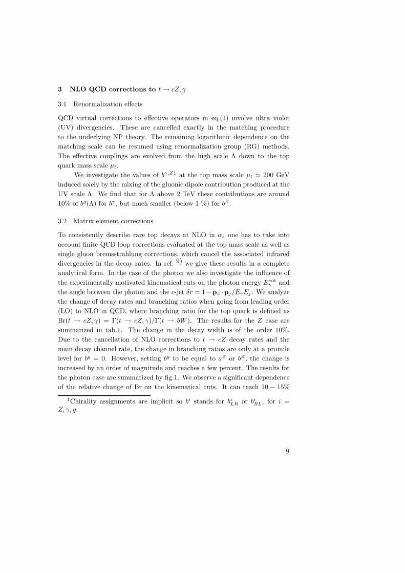
3 SUSY neutral bosons

SUSY incorporates two Higgs doublets, and after EWSB there are two neutral

bosons (H and A) in addition to the light Higgs. The mass of these two fields

is not EW, so they are naturally heavy enough to decay in tt. Their mass

difference depends on the µ parameter and the stop masses and trilinears in

addition to tanβ 7). Varying these parameters, for mA = 500 GeV we obtain

typical values of mH − mA between −2 and +10 GeV.

400 450 500 550 60015

16

17

18

19

20

21

22

�!!!!!s HGeVL

ΣHp

bL

400 450 500 550 60015

16

17

18

19

20

21

22

�!!!!!s HGeVL

ΣHp

bL

Figure 2: σ(gg → tt) for tanβ = 2 and SUSY bosons of mass mA = mH = 500GeV (left) or mA = 500, mH = 505 GeV (right). Dashes provide the narrow-

width approximation and dots the standard model cross section.

In fig.2-left we observe an average 5.5% excess and 8.1% deficit in the 5

GeV intervals before and after√

s = 500 GeV, respectively. There the position

of the peaks and dips caused by H and A overlap constructively. In contrast,

in fig.2-right their mass difference implies a partial cancellation between the

dip caused by A and the peak of H .

15

qq��

gg

-1.0 -0.5 0.0 0.5 1.00.0

0.2

0.4

0.6

0.8

1.0

cos Θ

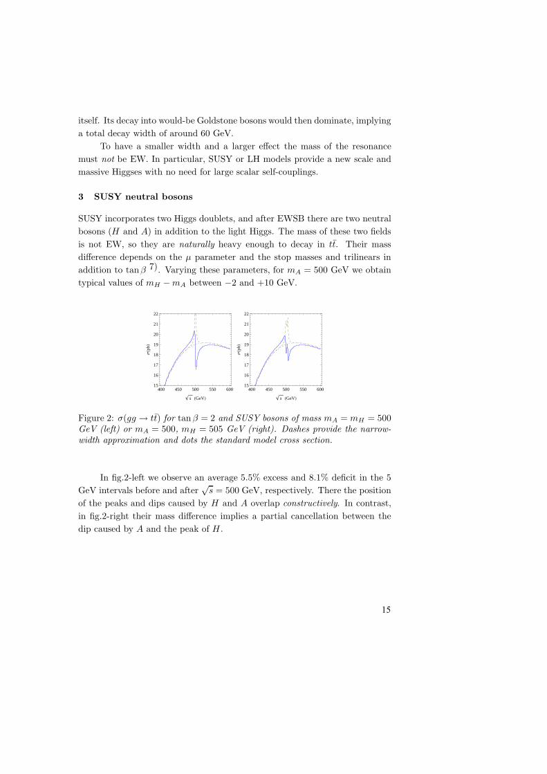
Figure 3: Standard angular distribution for the t quarks from qq and gg colli-

sions at√

s = 500 GeV. We include (dashes) the distribution from gg at the

peak and the dip of fig.2-left.

From fig.3 we argue that different cuts could be applied to reduce the

background for tt production at the LHC or even to optimize the contribution

from gg versus qq, but not to enhance the relative effect of the scalars on

σ(gg → tt).

4 Little Higgs boson

In LH models the Higgs appears as a pseudo-Goldstone boson of a global sym-

metry broken spontaneously at the scale f > v/√

2 = 174 GeV. The global

symmetry introduces an extra T quark and a massive scalar singlet r, the

Higgs of the symmetry broken at f . Once the electroweak VEV is included the

doublet and singlet Higgses mix 8, 9).

The extra Higgs r is somehow similar to the heavier scalar in a doublet

plus singlet model, with the doublet component growing with sθ = v/(√

2f).

If sθ is sizeable so is its coupling to the top quark. The coupling to the extra

T quark is stronger, but if r is lighter than 2mT then its main decay mode

will be into tt. Therefore, r is a naturally heavy (mr ≈ f) but narrow scalar

resonance with large couplings to quarks and an order one braching ratio to tt.

In 6) we examine this case in detail. The results are similar to the ones

obtained for SUSY bosons of the same mass.

16

5 Signal at the LHC

Let us now estimate the invariant mass distribution of tt events (mtt) in pp

collisions at the LHC. We will take a center of mass energy of 7 TeV and 1

fb−1 luminosity and we will not apply any cuts . At these energies the cross

section pp → tt is dominated by gg fusion (90%).

In fig.4 we observe a 5% excess followed by a 9% deficit, with smaller

deviations as mtt separates from the mass of the extra Higgs bosons. In fig.5

we find that changing the binning is important in order to optimize the effect.

.

.

Ev

en

ts

mtt [GeV]

540520500480460

3000

2800

2600

2400

2200

2000

1800

1600

1400

Figure 4: Number of tt events in pp collisions at 7 TeV and 1 fb−1 for mA =mH = 500 GeV and tanβ = 2 distributed in 5 GeV bins.

.

.

∆

mtt [GeV]

540520500480460

4

3

2

1

0

-1

-2

-3

-4

-5

.

.

∆

mtt [GeV]

540520500480460

4

3

2

1

0

-1

-2

-3

-4

-5

Figure 5: Deviation ∆ = (N − NSM)/√

NSM in the number of events respect

to the standard prediction for two different binning (mA = mH = 500 GeV and

tanβ = 2).

17

6 Summary and discussion

In models with an extended Higgs sector the extra bosons tend to have large

couplings with the top quark that imply a sizeable one-loop production rate at

hadron colliders. If the mass of these bosons is not EW but comes from a new

scale (e.g., the SUSY or the global symmetry-breaking scales), then they may

decay predominantly into tt. We have studied their effect on the tt invariant

mass distribution at 7 TeV and 1 fb−1. We have considered the deviations due

to the neutral bosons A and H of the MSSM, and to the scalar r associated to

the scale f in LH models. In all cases the interference dominates, invalidating

the narrow-width approximation.

References

1. A. Djouadi, Phys. Rept. 459 (2008) 1 [arXiv:hep-ph/0503173].

2. M. Schmaltz and D. Tucker-Smith, Ann. Rev. Nucl. Part. Sci. 55 (2005)

229.

3. M. Perelstein, Prog. Part. Nucl. Phys. 58 (2007) 247.

4. D. Dicus, A. Stange and S. Willenbrock, Phys. Lett. B 333 (1994) 126

[arXiv:hep-ph/9404359].

5. R. Frederix and F. Maltoni, JHEP 0901 (2009) 047 [arXiv:0712.2355 [hep-

ph]].

6. R. Barcelo and M. Masip, Phys. Rev. D 81 (2010) 075019 [arXiv:1001.5456

[hep-ph]].

7. W. de Boer, R. Ehret and D. I. Kazakov, Z. Phys. C 67 (1995) 647


8. R. Barcelo and M. Masip, Phys. Rev. D 78 (2008) 095012 [arXiv:0809.3124

[hep-ph]].

9. R. Barcelo, M. Masip and M. Moreno-Torres, Nucl. Phys. B 782 (2007)

159 [arXiv:hep-ph/0701040].

18



INCREASING THE LIGHTEST HIGGS MASS BOUNDOF THE MSSM

Paolo LodoneScuola Normale Superiore and INFN,

Piazza dei Cavalieri 7, 56126 Pisa, Italy

Abstract

In the MSSM the Higgs boson mass at tree level cannot exceed the Z bosonmass. One could then ask himself: should we throw away low energy Super-symmetry if we don’t see the Higgs boson at the LHC? To answer this questionit makes sense to consider extensions of the MSSM in which the Higgs bosoncan be relatively heavier. An additional motivation for looking in this direc-tion comes from flavour physics, since a heavier Higgs boson would relax thenaturalness bound on the masses of the sfermions of the first two generations,allowing them to be heavier and thus in better agreement with the absence ofany signal so far. We consider three possibile models from a bottom-up pointof view, and briefly discuss the phenomenological consequences.

19

1 Introduction

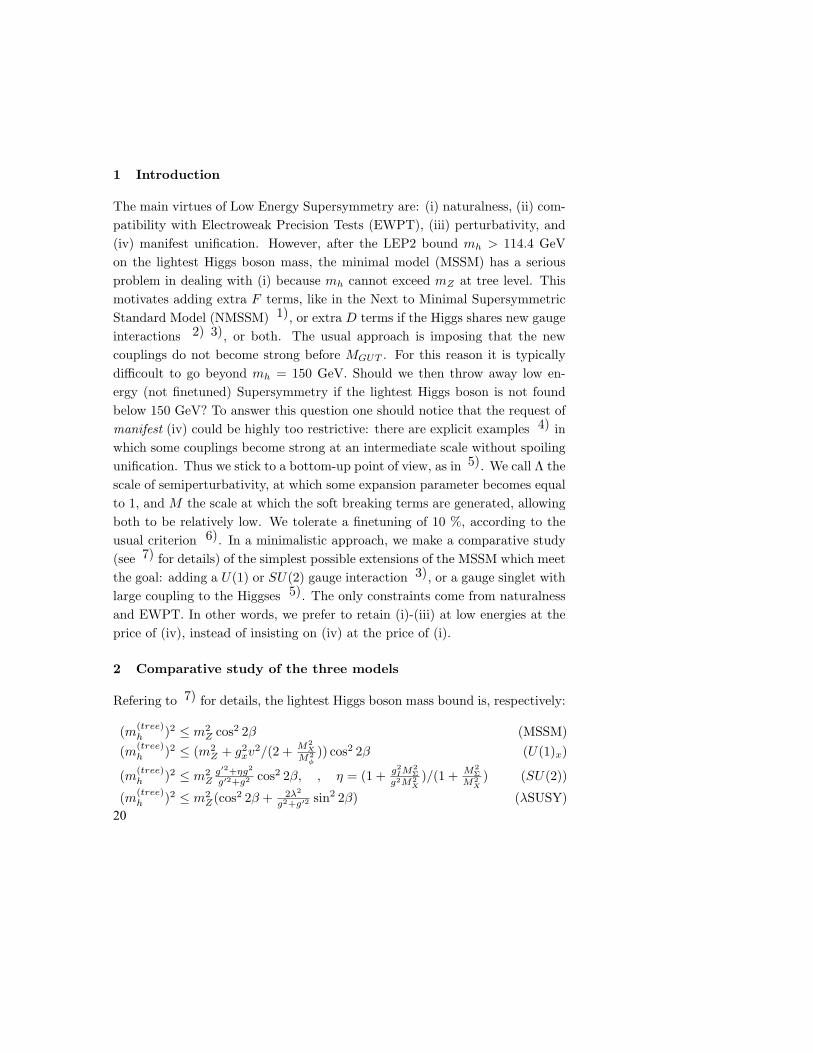
The main virtues of Low Energy Supersymmetry are: (i) naturalness, (ii) com-patibility with Electroweak Precision Tests (EWPT), (iii) perturbativity, and(iv) manifest unification. However, after the LEP2 bound mh > 114.4 GeVon the lightest Higgs boson mass, the minimal model (MSSM) has a seriousproblem in dealing with (i) because mh cannot exceed mZ at tree level. Thismotivates adding extra F terms, like in the Next to Minimal SupersymmetricStandard Model (NMSSM) 1), or extra D terms if the Higgs shares new gaugeinteractions 2) 3), or both. The usual approach is imposing that the newcouplings do not become strong before MGUT . For this reason it is typicallydifficoult to go beyond mh = 150 GeV. Should we then throw away low en-ergy (not finetuned) Supersymmetry if the lightest Higgs boson is not foundbelow 150 GeV? To answer this question one should notice that the request ofmanifest (iv) could be highly too restrictive: there are explicit examples 4) inwhich some couplings become strong at an intermediate scale without spoilingunification. Thus we stick to a bottom-up point of view, as in 5). We call Λ thescale of semiperturbativity, at which some expansion parameter becomes equalto 1, and M the scale at which the soft breaking terms are generated, allowingboth to be relatively low. We tolerate a finetuning of 10 %, according to theusual criterion 6). In a minimalistic approach, we make a comparative study(see 7) for details) of the simplest possible extensions of the MSSM which meetthe goal: adding a U(1) or SU(2) gauge interaction 3), or a gauge singlet withlarge coupling to the Higgses 5). The only constraints come from naturalnessand EWPT. In other words, we prefer to retain (i)-(iii) at low energies at theprice of (iv), instead of insisting on (iv) at the price of (i).

2 Comparative study of the three models

Refering to 7) for details, the lightest Higgs boson mass bound is, respectively:

(m(tree)h )2 ≤ m2

Z cos2 2β (MSSM)(m(tree)

h )2 ≤ (m2Z + g2

xv2/(2 + M2

X

M2φ

)) cos2 2β (U(1)x)

(m(tree)h )2 ≤ m2

Zg′2+ηg2

g′2+g2 cos2 2β, , η = (1 + g2IM

2Σ

g2M2X

)/(1 + M2Σ

M2X

) (SU(2))

(m(tree)h )2 ≤ m2

Z(cos2 2β + 2λ2

g2+g′2 sin2 2β) (λSUSY)20

where gx, gI and λ are new gauge and Yukawa couplings, MX is the mass ofthe new heavy vectors, and Mφ, MΣ are new soft masses.

First of all there must be compatibility with the EWPT. In the U(1) case,from the analysis 8) one can deduce MX & 5 TeV. For the SU(2) model weimpose MX/(5 TeV) & gX/g, where gX is the coupling of the triplet of heavyvectors. The case of λSUSY is thoroughly studied in 5) and shown to becompatible with data for low tanβ (≤ 3).

On the other hand there are constraints from the naturalness of the break-ing scale of the new gauge groups and of the Fermi scale. For the former wefix some ratios among parameters so that there is a tuning of no more than 10% at tree level, for the latter the amount of tuning can be shown to be given,in the interesting cases, by:

δm2Hu ≤

(m(tree)h )2

2×∆ (1)

where 1/∆ is the finetuning as defined by 6), and we accept ∆ = 10 atmost. From these conditions one obtains respectively lower bounds on theratios MX/Mφ,Σ and upper bounds on the soft masses Mφ and MΣ.

Putting all together one obtains the upper bound on mh at tree levelwhich is shown in Figure 1.

3 Phenomenological consequences

A unified discussion of the phenomenological consequences of this models ispresented in 9). Let us briefly mention some important points:

• Collider signatures: At least at the early stages of the LHC, taking Teva-tron into account, the most interesting signals come from gluino pairproduction. An effective way to characterize these signals is to considerthe semi-inclusive branching ratios:

BR(g → q1q2χ) (2)

where q1,2 stand for third generation quarks and χ stands for LSP plusW and/or Z bosons, real or virtuals. The final state would then be:

pp→ gg → q q q q + χχ (3) 21

2 4 6 8 10 120

100

200

300

400

log10HL�TeVL

mhm

axHG

eVL

Figure 1: Tree level bound on mh as a function of the scale Λ at which gI or λ orgX equals

√4π; for SU(2) (dashed), λSUSY (solid), and U(1) (dotdashed). For

λSUSY one needs tanβ . 3, in the other cases tanβ � 1 and 10% finetuningat tree level in the scalar potential which determines the new breaking scale. Inthe SU(2) case naturalness disfavours mh ≥ 270 GeV.

with q = top or bottom quarks. A particularly interesting signal are theequal sign dileptons from semi-leptonic decays.

An additional very much non-MSSM like signal would be the appearenceof the ‘golden mode’ h→ ZZ.

• Relic Dark Matter abundance: As is well known 10), after the LEP2bounds for the LSP to reproduce the observed dark matter abundanceone needs special relations among the parameters, which take the name of“well temperament”. For example for large SU(2) gaugino mass M2 �M1 one needs M1 ≈ µ, which looks like a finetuning problem. It isinteresting to notice that these special relations are significantly distortedin these models, mainly because of the increased lightest Higgs bosonmass.

• Flavour physics: Without degeneracy nor alignement the bounds that themasses of the squarks of the first two generations would have to satisfyare in the range of hundreds of TeV. Assuming an amount of degeneracyand alignement of the order of the Cabibbo angle and δRR � δLL, δLR orvice versa, one can see that even the strongest bounds can be satisfied if22

Table 1: Summary of the “performance” of the three models, see text.

Model mmaxh /mZ Price to pay

U(1) 2 (1),(2),(3)SU(2) 2 (3)SU(2) 3 (2),(3),(4)λSUSY 2 −λSUSY 3 (1)

mq1,2 & 10−20 TeV. In the MSSM this would introduce an unacceptablefinetuning on the Fermi scale. On the contrary, if the lightest Higgsboson mass is significantly increased at tree level, there can be room forthese values compatibly with naturalness. From this respect, the mostpromising possibility is λSUSY.

4 Conclusions

From a bottom-up point of view, the lightest Higgs boson mass can be sig-nificantly raised at tree level. Constraints come from the interplay betweennaturalness and experimental constraints. The maximum possible mh that onecan obtain is shown in Figure 1 as a function of the scale of semiperturbativity.In the SU(2) case it seems difficoult to be consistent with both the EWPTand naturalness if mh is beyond 270 GeV. The prices that one may have topay are the following: (1) low semiperturbativity scale Λ; (2) low “messenger”scale M at which the soft terms are generated; (3) presence of different scalesof soft masses; (4) need for extra positive contributions to T . With low scalewe mean . 100 TeV, with (3) we mean that, besides the usual soft masses oforder of hundreds of GeV, one may need some new soft masses of order 10 TeV.The “performance” of the three models is summarized in Table 1. A unifiedviewpoint on the Higgs mass and the flavor problem for this kind of modelsand other phenomenological consequences are discussed in 9).

5 Acknowledgments

I thank Enrico Bertuzzo, Marco Farina, and especially Riccardo Barbieri.

23

References

1. P. Fayet, Nucl. Phys. B 90, 104 (1975).J. R. Ellis et al, Phys. Rev. D 39, 844 (1989).M. Drees, Int. J. Mod. Phys. A 4, 3635 (1989).

2. H. E. Haber and M. Sher, Phys. Rev. D 35, 2206 (1987).J. R. Espinosa and M. Quiros, Phys. Lett. B 279, 92 (1992).J. R. Espinosa and M. Quiros, Phys. Rev. Lett. 81, 516 (1998) arXiv:hep-ph/9804235.

3. P. Batra et al, JHEP 0402, 043 (2004) arXiv:hep-ph/0309149.

4. R. Harnik et al, Phys. Rev. D 70, 015002 (2004) arXiv:hep-ph/0311349.S. Chang et al, Phys. Rev. D 71, 015003 (2005) arXiv:hep-ph/0405267.A. Birkedal et al, Phys. Rev. D 71, 015006 (2005) arXiv:hep-ph/0408329.

5. R. Barbieri et al, Phys. Rev. D 75, 035007 (2007) arXiv:hep-ph/0607332.

6. R. Barbieri and G. F. Giudice, Nucl. Phys. B 306, 63 (1988).

7. P. Lodone, JHEP 1005 (2010) 068 arXiv:1004.1271.

8. E. Salvioni et al, arXiv:0911.1450; .E. Salvioni et al, JHEP 0911, 068 (2009) arXiv:0909.1320.

9. R. Barbieri et al, arXiv:1004.2256.

10. N. Arkani-Hamed et al, Nucl. Phys. B 741 (2006) 108, arXiv:0601041.

24



STUDY OF W+JETS BACKGROUND TO TOP QUARK PAIR

PRODUCTION CROSS SECTION IN ATLAS AT THE LHC

Maria Ilaria BesanaUniversita degli Studi di Milano and INFN Milano

Abstract

The measurement of top quark pair production cross section in p-p collisionsat center-of-mass energy of 7 TeV is one of the first measurements that will bemade by ATLAS at the LHC. The most promising channel is the semileptonicfinal state, where one of the top decays into a W decaying into hadrons andthe other top into a W decaying leptonically. The dominant background tothis channel of top quark pairs is given by direct p-p production of W+jets.Monte Carlo predictions for the rate of this background have large uncertain-ties; however it will be important to know it with precision in order to makean accurate measurement of top quark pair production cross section. In thefollowing, a data-driven technique developed in order to reduce this uncertaintyis presented and first results on real data are discussed.

25

1 Introduction

The top quark discovery at Fermilab in 1995 completed the three generation

structure of the Standard Model (SM) and opened the new field of top quark

physics. After QCD jets, W and Z bosons, the production of top quarks is the

dominant process in p-p collisions at multi-TeV energies. The LHC would be a

top quark factory: top quark pair production cross section at LHC is expected

to be enhanced by a factor 20 with respect to Tevatron even at 7 TeV. Top

quark physics is a rich subject. Top quark events are indeed very useful for

detector commissioning and they can provide a consistency test of Standard

Model. The knowledge of top quark production cross section is also crucial,

because it can be a significant background to events predicted by some models

beyond the Standard Model.

This report will concentrate on the measurement of top quark pair pro-

duction cross section in the early stage of data taking, i.e. with the amount of

data expected to be collected in 2010. Event selection cuts and expected num-

bers of candidate events with an integrated luminosity of 10 pb−1 are reported

in Section 2. A data-driven technique for the estimation of the dominant back-

ground process, W+jets, is discussed in Section 3. Finally first results on 7

TeV data collected by ATLAS detector are reported in Section 4.

2 Selection of top quark pairs events

In Standard Model, top quarks decay takes place almost exclusively through

the t → Wb decay mode. A W-boson decays in about 1/3 of the cases into

a charged lepton and a neutrino. All three lepton flavors are produced at an

approximately equal rate. In the remaining 2/3 of the cases, the W+-boson

decays into an up-type quark and a down-type anti-quark pair 1. Since the

CKM matrix suppresses decays involving b-quarks as |Vcb|2 ≃ 1.7 10−5, W-

boson decay can be considered as a clean source of light quarks (u,d, s,c). Top

quark pairs decay modes are then classified into:

• fully leptonic, if both W’s decay leptonically,

• fully hadronic, if both W’s decay into hadrons,

• semileptonic, if a W decays into leptons and the other one into hadrons.

1Charge coniugate states are implicitly included through the paper.

26

Table 1: Expected number of selected events at 7 TeV with an integrated lumi-

nosity of 10 pb−1 both of signal and main backgrounds.

Sample Electron channel Muon channel

top quark pairs 53 65W+jets 29 40

single top 5 5other backgrounds 6 6

Semileptonic channel is very interesting, because of good branching ratio

(45%) and clear experimental signature. The final state is indeed characterized

by one energetic lepton, at least four energetic jets (initial and final state gluon

radiation often increases the number of final state jets) and missing transverse

energy (EmissT ), because of the neutrino. Finally invariant mass of three of

these jets is equal to top quark mass. Top quark pairs events in semileptonic

channel are selected requiring exactly one lepton (electron or muon 2) with

transverse momentum pT > 20 GeV and absolute value of pseudorapidity

|η| < 2.5, EmissT > 20 GeV and at least 4 jets with transverse momentum

pT > 20 GeV and |η| < 2.5. Finally we require that 3 of these jets have

transverse momentum pT > 40 GeV. Electrons and jets are measured using

calorimeters and inner tracker. Missing transverse energy is a complex quantity,

because of the use of information from the whole detector. It is calculated from

the sum of energy of all particles seen in the detector:

EmissT =

√(Emiss

x )2 + (Emissy )2 Emiss

i = −ΣEi with i = x, y (1)

2.1 Expected number of selected events with an integrated luminosity of 10pb−1

The signal and major backgrounds have been estimated from Monte Carlo

simulations which include a full simulation of the ATLAS detector. Table

1 summarises the expected numbers of signal and background events for the

electron and muon channel analysis, namely the direct W+jets production

from p-p collisions, single top production and other backgrounds as Z+jets

production, dibosons production and top quark pair decaying fully hadronically.

The dominant expected background is W+jets direct production from

p-p collision and it is very dangerous. W+jets events can have indeed the

2Single lepton channel with tau lepton needs a dedicated analysis.

27

same experimental signature of top quark pairs events. The cross section for

associated production of W and 4 hadronic jets is non negligible at the LHC

(≃350 pb at 7 TeV). W+jets cross section has a big uncertainty, up to 100%

for W+4jets. There is not indeed NLO calculation for the cross section of this

process and Monte Carlo predictions are based on parameters estimated for

energy 4 times lower than the LHC one. Finally, it is very difficult to measure

it directly from data because of big top quark contamination. Estimation of

this background is however crucial in order to have a precise measurement of

top quark pair production cross section. A data-driven technique, described in

the next section, has been developed for this purpose.

3 Data-driven technique for W+jets background estimation

W+jets can be estimated with a data-driven technique based on the fact that W

to Z ratio is predicted with a much smaller uncertainty 1) 2) than W+jets cross

section. Since the jet multiplicity distribution for Z events can be measured

with data, this observation can be used to reduce the Monte Carlo uncertainty

on the fraction of W+jets present in the selected sample of candidate top events.

The idea is to extrapolate from a control region (CR) with one jet into the top

signal region (SR) with four or more jets and estimate the number of W+jets

background events using the formula:

WSR = CMC ∗ZSR

ZCR∗ WCR where CMC =

(ZCR

WCR

)

MC

(2)

where WCR and ZCR represent the number of W and Z candidates re-

constructed in the low jet multiplicity control region. ZSR is the number of

candidate Z events which pass the same selection criteria as those imposed in

the top-antitop analysis (top quark signal region). CMC is a coefficient deter-

mined from Monte Carlo, which takes into account mass difference between W

and Z bosons. Z → ee (Z → µµ) candidate events are selected (after the trig-

ger) by requiring two electrons (muons) of opposite charge, with an invariant

mass between 80 GeV and 100 GeV. ZSR sample is selected by applying the

default baseline analysis selection, i.e. requiring three jets with pT above 40

GeV, a fourth with pT greater than 20 GeV and |η| < 2.5. Events in control

region are selected asking exactly one jet of transverse momentum pT >20 GeV

and |η| < 2.5.

28

3.1 Main sources of uncertainty

There are three main sources of uncertainty for this method. The first one is

the uncertainty on CMC. This has been estimated comparing different Monte

Carlo generators and varying their parameters and was found to be 12% both in

electron and muon channel. Another source of uncertainty comes from back-

ground contamination to WCR. The dominant background is QCD di-jets

production. Estimation of its contribution from data is ongoing. At present a

conservative assumption was done that it will be possible to estimate it with

an accuracy of 50%. Its contribution on W+jets background estimation uncer-

tainty is 16% in electron channel and 13% in muon channel. Finally statistical

uncertainty is dominated by the number of expected Z events in signal re-

gion. It is reduced combining electron and muon channels for Z events , since

ZSR/ZCR is independent from lepton flavor. The number of W events in top

quark signal region can be estimated as:

WSR = CMC ∗ZSR → ee + ZSR → µµ

ZCR → ee + ZCR → µµ∗ WCR (3)

Taking into account all these sources of uncertainty, W+jets background

uncertainty will be reduced to 50% with first 10 pb−1; this is a significant

improvement with respect to Monte Carlo predictions. The contribution of the

W+jets background uncertainty to the uncertainty on top quark cross section

measurement will be 25%. After an integrated luminosity of 100 pb−1, the

uncertainty on W+jets background estimation will be reduced to 20%.

4 Analysis on real data

ATLAS detector started to take collision data at 7 TeV on March 30th, 2010.

At the time of this report (June 2010) with data corrisponding to integrated

luminosities of 6.7 nb−1 and 6.4 nb−1 in the electron and muon channels re-

spectively, 17 W → eν and 40 W → µν candidates were selected. One Z → ee

and two Z → µµ candidates were also observed, resulting from total integrated

luminosities of 6.7 nb−1 and 7.9 nb−1, respectively. W and Z candidate events

were selected as reported in Section 3. An higher cut on EmissT was applied for

W candidates selection in order to suppress QCD background contamination

(25 GeV instead of 20 GeV). No requirements on associated jets were applied.

Figures 1 shows transverse mass (mT) of W candidates and compares it to

signal and background Monte Carlo samples. It is clear the presence of signal

over the background. Analysis on real data is ongoing. With a luminosity of

29

few nb−1, W/Z ratio can be studied at low jet multiplicity and QCD di-jets

contamination to WCR sample can be estimated

[GeV] Tm

0 20 40 60 80 100 120

Ent

ries

/ 5 G

eV

-210

-110

1

10

210

310 = 7 TeV )sData 2010 (

ν e→W

QCD

ντ →W

PreliminaryATLAS

-1

L = 6.7 nb∫

0 20 40 60 80 100 120-210

-110

1

10

210

310

0 20 40 60 80 100 120-210

-110

1

10

210

310

(a)

[GeV]Tm

0 20 40 60 80 100 120

Ent

ries

/ 5 G

eV-110

1

10

210

310

[GeV]Tm

0 20 40 60 80 100 120

Ent

ries

/ 5 G

eV-110

1

10

210

310ATLAS Preliminary

-1 L = 6.4 nb∫

= 7 TeV)sData 2010 (

νµ →W

QCD

ντ →W

µµ →Z

(b)

Figure 1: Transverse mass of W candidates in electron (a) and muon (b) chan-

nel. Expectation from Monte Carlo are compared with data.

5 Conclusions

It is crucial for the measurement of the top quark cross section to reduce the

uncertainty on the expected number of W+jets background events. The data-

driven technique presented here allows to reduce this uncertainty by a factor

two even with first 10 pb−1. Selection cut optimization is ongoing in order to

reduce the systematic uncertainty coming from QCD di-jets contamination to

WCR and statistical uncertainty coming from the number of Z events in signal

region.

References

1. F. A. Berends, W. T. Giele, H. Kuijf, R. Kleiss, W. J. Stirling, Physics

Letters B 224, (1989) 237.

2. E. Abouzaid, H. Frisch, Phys. Rev. D 68 (2003) 033014.

30



MONITORING THE Mrk421 FLARING ACTIVITY

BY THE ARGO-YBJ EXPERIMENT

Roberto IuppaINFN, Sezione Roma Tor Vergata

Dipartimento di Fisica, Universita di Roma Tor Vergataon behalf of the ARGO-YBJ collaboration

Abstract

ARGO-YBJ is an extensive air shower detector exploiting the full coverageapproach at high altitude (4300 m a.s.l.), designed for gamma-ray astronomyand cosmic-ray physics in the 300 GeV - 30 TeV energy range. One of the mostintense gamma-ray sources detected by ARGO-YBJ is Mrk421. It is a blazarclose to the Earth (redshift: z = 0.031), intensively studied because of itshighly varying flaring activity. During the last four years, three major flaringperiods have been observed by ARGO-YBJ, in July 2006, in June 2008 and inFebruary 2010. Thsee flares show interesting spectral features, mostly as faras the relation between the X-ray and the gamma-ray emissions is concerned.The status of the observation of Mrk421 is reported.

31

1 Introduction

In 1992 the blazar Markarian 421 (Mrk421) became the first extragalactic

source observed at gamma-ray energy E > 500GeV 1). It is classified as a

radio-loud active galactic nucleus (AGN), a subclass of BL Lacertae objects

(BL Lac), characterized by a non-thermal spectrum extending up to high en-

ergies and by rapid flux variability at nearly all wavelengths. So far, Mrk421

is the closest BL Lac detected above 100 GeV (z = 0.031), making it the most

studied TeV-emitting AGN and the main benchmark for each model on the

emission processes in AGNs and the attenuation of TeV gamma rays propagat-

ing through extragalactic space.

The flaring activity of Mrk421 spans over twelve decades of energy (from

optical to TeV) and has been observed with variability timescales ranging from

minutes to months. Such physical properties require data merging from differ-

ent experiments in order to get observations as complete as possible.

TeV detection is especially challenging, because of the low emission rate

and the short duration of most flares. Nonetheless, many efforts have been

spent to observe Mrk421 at TeV energies, because these measurements provide

important indications on the source properties and the radiation processes.

Recently, several multiwavelength campaigns have revealed a strong correlation

of gamma rays with X-rays, that can be easily interpreted in terms of the

Synchrotron Self-Compton model 2) 3). Altough significant variations of the

TeV spectrum slope during different activity phases still remain unexplained,

some hints have been found of the correlation between the spectral hardness

and the flux intensity 4).

Since the emission flux at Very High Energy (VHE, above 100 GeV) is

rather low, detections must be carried out with ground-based experiments, with

large effective area. In addition, the strong variability of the flaring phenomena

demands high duty-cycle and large field of view.

The ARGO-YBJ experiment, located at the Yangbajing Cosmic Ray Lab-

oratory (Tibet, 4300 m a.s.l., 30◦ 0′38′′N, 90◦ 3′50′′E), since 2007 December has

been performing a continuous monitoring of the sky in the declination band

from −10◦ to 70◦. The detector was taking data also during summer 2006, and

the ARGO-YBJ dataset represents a unique chance to report on the Mrk421

activity during the last four years.

32

2 The ARGO-YBJ experiment

The ARGO-YBJ detector, located at the Yangbajing Cosmic Ray Laboratory

(Tibet, P.R. China, 4300 m a.s.l.), is the only experiment exploiting the full

coverage approach at very high altitude. The detector is composed of a central

carpet ∼74×78 m2, made of a single layer of Resistive Plate Chambers (RPCs)

with ∼92% of active area, enclosed by a partially instrumented guard ring that

extends the detector surface up to ∼100×110 m2, for a total active surface of

∼6700 m2. The apparatus has a modular structure, described in 5).

The spatial coordinates and the arrival time of any detected particle are

used to reconstruct the position of the shower core and the arrival direction of

the primary 6).

The ARGO-YBJ experiment started recording data with the whole cen-

tral carpet in June 2006. Since 2007 November the full detector has been in

stable data taking (trigger particle multiplicity Ntrig =20) with a duty cycle

∼ 90%. The trigger rate is about 3.6 kHz.

3 Signal maps

Showers induced by VHE photons coming from Mrk421 are collected when the

source zenith angle with respect to Yangbajing is less than 40◦. Extending

the analysis beyond such limit would slightly increase the exposure time, but

a general worsening of the angular resolution should be faced and the energy

resolution would be poorer. Since the ratio signal/noise within 1◦ from the

source is about 10−4 ÷ 10−5, a reliable method of background estimation is

needed. The ARGO-YBJ successfully applied different background estimation

techniques, each of them giving results consistent with the others.

In order to resolve the primary photons energy, the dataset is divided into

multiplicity ranges, according to how many pads the induced shower fires on

the central carpet. Fig. 1 reports the cumulative signal detected by ARGO

until February 2010, obtained with showers having multiplicity greater than 60.

As anticipated in the introduction, the importance of Mrk421 rests basically

in the strong variability of its emission. During the last four years, several

flares lasting up to tens of days occurred. A short description of the results

concerning each flare follows.

33

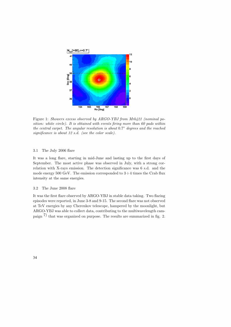
Figure 1: Showers excess observed by ARGO-YBJ from Mrk421 (nominal po-

sition: white circle). It is obtained with events firing more than 60 pads within

the central carpet. The angular resolution is about 0.7◦ degrees and the reached

significance is about 12 s.d. (see the color scale).

3.1 The July 2006 flare

It was a long flare, starting in mid-June and lasting up to the first days of

September. The most active phase was observed in July, with a strong cor-

relation with X-rays emission. The detection significance was 6 s.d. and the

mode energy 500 GeV. The emission corresponded to 3÷4 times the Crab flux

intensity at the same energies.

3.2 The June 2008 flare

It was the first flare observed by ARGO-YBJ in stable data taking. Two flaring

episodes were reported, in June 3-8 and 9-15. The second flare was not observed

at TeV energies by any Cherenkov telescope, hampered by the moonlight, but

ARGO-YBJ was able to collect data, contributing to the multiwavelength cam-

paign 7) that was organized on purpose. The results are summarized in fig. 2.

34

Figure 2: Energy spectrum of Mrk421 emission as measured by ARGO-YBJ. It

is compared with recent theoretical predictions and previous measurements 8).

3.3 The February 2010 flare

On February, 16th 2010, it took ARGO-YBJ only 6 hours to detect a 5 s.d.

significant signal from Mrk421. Positive detections occurred in the following

three days too. It was the first time an array-like EAS experiment reached such

sensitivities in γ-ray astronomy. Altough further analyses are needed to take

conclusions, the energy spectrum looked exceptionally softer, thus feeding the

discussion in 4).

4 Correlations with X-ray emission

Fig. 3 illustrates the correlation between the TeV emission from Mrk421 ob-

vserved by ARGO-YBJ and the X-rays fluxes reported by satellites in the same

time. Both plots report the cumulative event rate from ARGO-YBJ as a func-

tion of time (red points). Integral fluxes in soft (left plot) and hard X-ray (right

plot) are also reported (black lines). There is evidence that the VHE signal

is more correlated with the hard X component than with the soft X. Deeper

studies are in progress to understand the implications of such observations on

the emission models.

5 Conclusions

ARG0-YBJ successfully monitored the VHE emission of Mrk421 over the last

four years. In this period, three major flaring phases were observed, down to

daily timescale, completing the experimental dataset available to the scientific

35

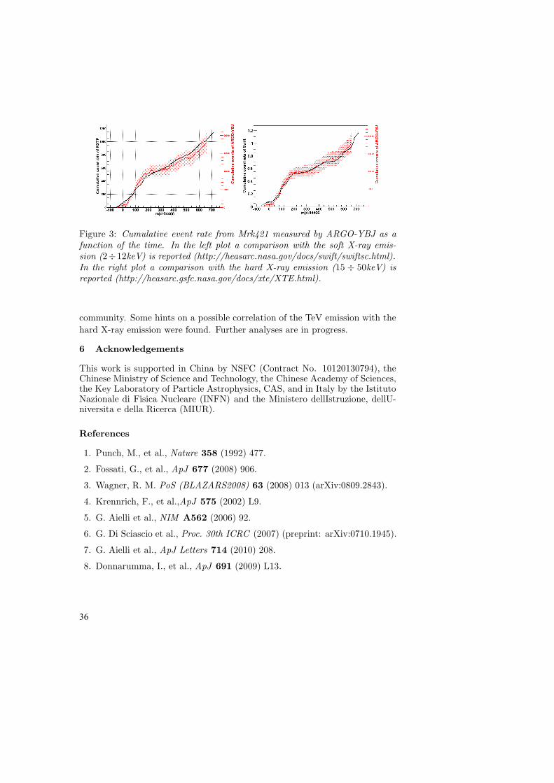
Figure 3: Cumulative event rate from Mrk421 measured by ARGO-YBJ as a

function of the time. In the left plot a comparison with the soft X-ray emis-

sion (2÷12keV) is reported (http://heasarc.nasa.gov/docs/swift/swiftsc.html).

In the right plot a comparison with the hard X-ray emission (15 ÷ 50keV) is

reported (http://heasarc.gsfc.nasa.gov/docs/xte/XTE.html).

community. Some hints on a possible correlation of the TeV emission with the

hard X-ray emission were found. Further analyses are in progress.

6 Acknowledgements

This work is supported in China by NSFC (Contract No. 10120130794), theChinese Ministry of Science and Technology, the Chinese Academy of Sciences,the Key Laboratory of Particle Astrophysics, CAS, and in Italy by the IstitutoNazionale di Fisica Nucleare (INFN) and the Ministero dellIstruzione, dellU-niversita e della Ricerca (MIUR).

References

1. Punch, M., et al., Nature 358 (1992) 477.

2. Fossati, G., et al., ApJ 677 (2008) 906.

3. Wagner, R. M. PoS (BLAZARS2008) 63 (2008) 013 (arXiv:0809.2843).

4. Krennrich, F., et al.,ApJ 575 (2002) L9.

5. G. Aielli et al., NIM A562 (2006) 92.

6. G. Di Sciascio et al., Proc. 30th ICRC (2007) (preprint: arXiv:0710.1945).

7. G. Aielli et al., ApJ Letters 714 (2010) 208.

8. Donnarumma, I., et al., ApJ 691 (2009) L13.

36



STUDY OF THE DECOHERENCE OF ENTANGLED KAONS

BY THE INTERACTION WITH THERMAL PHOTONS

Izabela BalwierzJagiellonian University, Institute of Physics, Krakow, Poland

Wojciech WislickiA. Soltan Institute for Nuclear Studies, Warszawa, Poland

Pawel MoskalJagiellonian University, Institute of Physics, Krakow, Poland

Abstract

The KLOE-2 detector is a powerful tool to study the temporal evolution ofquantum entangled pairs of kaons. The accuracy of such studies may in princi-ple be limited by the interaction of neutral kaons with thermal photons presentinside the detector. Therefore, it is crucial to estimate the probability of thiseffect and its influence on the interference patterns. In this paper we intro-duce the phenomenology of the interaction of photons with neutral kaons andpresent and discuss the obtained quantitative results.

1 The interaction frequency between thermal photons

and neutral kaons

Interaction between K0 meson and thermal photons may remain undetected

inside the KLOE-2 detector and constitute the background process where quan-

tum coherence is destroyed.

37

To estimate the probability of this interaction, we assume in the calcula-

tions that photons are in a room temperature and K0 is moving with respect

to the laboratory frame with the energy obtained in the φ → K0K0 decay.

Meson K0 is electrically neutral but it has inner electromagnetic structure

so it can interact with photons. We are interested in interactions in which K0 is

observed in a final state. The main process is the inverse Compton effect, that

is photon scattering on kaon in which photon’s energy increases and kaon’s

decreases. The total number of photons scattered on a kaon in time unit is

given by:

dN

dt=

1

γ

dN∗

dt∗=

c

γ

∫dn∗σ∗

γK(k∗), (1)

where γ is the Lorentz factor, c the velocity of light and σγK denotes the cross

section for γK0 Compton scattering. Superscript ,,∗” indicates the rest frame

of K0 meson. We denote by dn number of photons in unit of volume in the dk

energy interval, given by:

dn =1

4π3·k2dkdφ sin θdθ

ek

kB T − 1. (2)

The above formula was obtained assuming that the photon distribution is given

by the Planck’s law of black-body radiation in the temperature T. Here θ stands

for the polar angle between the incoming photon and the velocity of kaon, and

kB is the Boltzmann constant.

The cross section σγK for the γK0 Compton scattering can be obtained

from the cross section for the radiative scattering of the kaon in electromagnetic

fields of nuclei, known as the Primakoff effect, and is given by 1):

dσ∗

γK(k∗, θ∗)

d cos θ∗=

2παf

mK

k∗2

(αK(1 + cos2 θ∗) + 2βK cos θ∗

)

(1 + k∗

mK

(1 − cos θ∗))3

, (3)

where mK is the K0 mass and αf the fine-structure constant. The αK and

βK stand for the electric and magnetic polarizability of K0. These quantities

characterize susceptibility of the K0 to the electromagnetic field. Taking into

account the Lorentz transformation of the photon energy from the laboratory

frame to the rest frame of K0:

k∗ = γk(1 − β cos θ)) (4)

38

and the Lorentz invariance of dn/k, one gets the transformation of the density

of photons:

dn∗ = dn(1 − β cos θ)γ, (5)

where β is the velocity of K0 with respect to the laboratory frame. Using

consecutively equations (5), (2) and (4) and knowing that∫ 2π

0dφ = 2π, the

formula for the interaction frequency (1) reads (where u = cos θ):

dN

dt=

c

2π2

∫∞

0

dkk2

ek

kB T − 1

∫ 1

−1

du · (1 − βu) · σ∗

γK(γk(1 − βu)). (6)

2 Units and values of parameters

Numerical values of parameters αK and βK used in equations in the last para-

graph are equal to αK = 2.4 · 10−49 m3 and βK = 10.3 · 10−49 m3 2). Values

for αf , mK , kB and c are taken from Particle Data Group 3). Temperature is

assumed to be 300K.

In natural units, the conversion eV → m should be done in the following

way: eV = (197.33 · 10−9 m)−1, so the unit of (6) is:

[dN

dt

]= m4

· eV4·1

s= 6.595 · 1026 1

s. (7)

In the case of the φ → K0K0 decay the kinetic energy of kaons in the

laboratory frame is equal to ca. E = 12 MeV, corresponding to:

γ = E+mK

mK

= 1.02412, β =√

1 − 1

γ2 = 0.21573.

3 Calculation of the cross section for inverse Compton scattering

of γ on K0

The total cross section σγK may be obtained by integrating (3) over the cos θ∗.

In order to simplify the calculations we will introduce the notation cos θ∗ = x

and u = −m − k∗ + k∗x:

σ∗

γK(k∗, u) = 2παfm2

(αK

∫−k∗2 − (m + k∗)2 − u2 − 2u(m + k∗)

k∗u3du +

+ 2βK

∫−m− k∗ − u

u3du

). (8)

39

After calculating σ∗

γK(k∗, u) and replacing u = −m−k∗+k∗x, we integrate

it over x in the interval [−1, 1]. As a result we get:

σ∗

γK(k∗) = σ∗

γK(k∗, x |1−1) =

2παf

k∗(m + 2k∗)2

(2k∗(2(αK + βK)k∗3 +

− 3αKm2k∗− αKm3) + αKm2(2k∗ + m)2(ln

m + 2k∗

m)). (9)

4 Calculation of interaction frequency

Now we put equation (9) from the previous section into formula for dNdt

(6).

The integrand for dNdt

, multiplied by the unit conversion constant (7), is shown

in Figure 1.

0.1 0.2 0.3 0.4photon energy @eVD

5.´10-31

1.´10-30

1.5´10-30

2.´10-30

2.5´10-30

integrand for dN�dt HkL

Figure 1: Integrand for dNdt

(k)

Finally integrating numerically dNdt

over k we obtain:

dN

dt= 3.7 · 10−31 1

s

4.1 Numerical stability

Integral calculated in this chapter is quite sensitive to the numerical accuracy

and have to be treated with caution. The graph below shows the value of

the whole integral dNdt

(6) with respect to the numerical precision (number of

significant digits). One can see from it, that when we reach sufficient precision,

the result stabilizes.

40

28 30 32 34 36number of significant digits

5.´10-32

1.´10-31

1.5´10-31

2.´10-31

2.5´10-31

3.´10-31

3.5´10-31

value of intergal dN�dt

Figure 2: Value of integral dN/dt

4.2 Investigation on systematic errors

Although the interaction probability is small, the systematic error on it was

estimated. Obvious sources of systematics are uncertainty of αK and βK and

variation of temperature.

The first one was estimated using values of αK and βK , derived using

different methods in papers 4) and 5). The result obtained in this paragraph

was calculated using kaon polarizabilities taken from the paper 2). Points on

the graph 3a correspond to the different combinations of αK and βK . Figure

3b illustrates how the result changes due to the room temperature variations

in the range of 20K around value of 300K.

0 2 4 6 8No.

2.´10-31

4.´10-31

6.´10-31

value of intergal dN�dt

290 295 300 305 310T @KD

3.2´10-31

3.4´10-31

3.6´10-31

3.8´10-31

4.´10-31

4.2´10-31

4.4´10-31value of intergal dN�dt

Figure 3: a) Values of integral for different αK and βK parameters. b) Values

of integral as a function of temperature.

Depending on the assumed values of αK , βK and temperature, the dNdt

varies from about 5·10−32 to 7.5·10−31 so by more than one order of magnitude.

However, as we will see in the next paragraph, this difference is not significant

for the parameters of decoherence of kaon pairs at KLOE-2 detector.

41

5 Physical interpretation

Kaon is moving with velocity equal to ca. v = 0.6 · 108 ms with respect to the

laboratory frame. From the place of its creation to the calorimeter it moves

through about 2.5m so it needs for it about 4.2 · 10−8s. Because the frequency

of the Compton interaction is 3.7 · 10−31 1

s so probability of the interaction is:

P = 1.5 · 10−38

This background stays small with respect to the statistical uncertainty of de-

coherence parameters expected in KLOE-2 6).

6 Acknowledgements

We acknowledge support by Polish Ministry of Science and Higher Education

through the Grant No. 0469/B/H03/2009/37.

References

1. M.A. Moinester, V. Steiner, e-Print: arXiv:hep-ex/9801008v3, 7 (1998).

2. D. Ebert, M.K. Volkovy, T. Feldmann, Intern. Journal of Modern Phys. A

12, 4408 (1997).

3. Particle Data Group: http://pdg.lbl.gov

4. J. Christensen, W. Wilcox, F.X. Lee, L. Zhou, Phys. Rev. D 72, 9-10

(2005).

5. M. A. Ivanov, T. Mizutani, Phys. Rev. D 45, 1590 (1992).

6. G. Amelino-Camelia et al., e-Print: arXiv:1003.3868v3 [hep-ex], 14 (2010).

42



INVESTIGATIONS OF THE TIME INTERVAL

DISTRIBUTIONS BETWEEN THE DECAYS OF QUANTUM

ENTANGLED NEUTRAL KAONS

Tomasz TwarógJagiellonian University, Institute of Physics, Kraków, Poland

Abstract

One of the physics issues to be investigated in KLOE-2 experiment 1) is the timeevolution of quantum entangled neutral kaons. Studies of kaons’ decay timesdistributions enable us to test CPT symmetry and quantum mechanics (QM).In this article it is shown how these distributions can be obtained on the basis ofQM. It is also discussed how CPT and QM violations can manifest themselvesin the interference patterns of entangled kaons which will be measured by meansof the KLOE-2 detector setup.

1 Introduction

Neutral kaons were particles for which CP 2) and T 3) violations were first

observed. Then it should not come as a surprise that they are promising can-

didates in the search of CPT noninvariance. At the same time neutral kaons

enable us to test QM, for instance through decoherence tests.

43

2 Hamiltonian

Neutral kaon’s time evolution can be described as:

|K (t)〉 = a (t)∣∣K0

⟩+ b (t)

∣∣K0⟩

+∑

j

cj (t) |fj〉 , (1)

where the sum is over all final states |fj〉 a kaon may decay to and functions a

and b obey the Schrödinger-like equation with effective Hamiltonian H: 4)

i∂

∂t

(a (t)b (t)

)= H

∂

∂t

(a (t)b (t)

). (2)

H can be divided into its hermitian and antihermitian parts:

H = M −i

2Γ =

(M11 M12

M∗

12 M22

)−

i

2

(Γ11 Γ12

Γ∗

12 Γ22

), (3)

where M and Γ are hermitian and are called mass and decay matrices. The

eigenvectors of H are found to be: 4)

|KS〉 =1√

2 (1 + |ǫ2S |)·[(1 + ǫS)

∣∣K0⟩

+ (1 − ǫS)∣∣K0

⟩],

|KL〉 =1√

2 (1 + |ǫ2L|)·[(1 + ǫL)

∣∣K0⟩− (1 − ǫL)

∣∣K0⟩]

.

(4)

Here ǫS and ǫL are two small parameters measuring CP violation. One can

define another two variables:

ǫdef==

ǫS + ǫL

2, δ

def==

ǫS − ǫL

2. (5)

Parameter ǫ measures average CP violation for KL and KS, while δ is a CPT -

violating parameter.

3 Final states amplitudes and double decay rate

At KLOE, neutral kaons are produced in Φ meson decay, JPC = 1−−. To

conserve the eigenvalues of P and C, the (normalized) initial state of the two

kaons, written in the Φ rest frame, has to be:

|i〉 =1√

2{∣∣K0 (−~p)

⟩ ∣∣K0 (+~p)⟩−

∣∣K0 (−~p)⟩ ∣∣K0 (+~p)

⟩} = (6)

=N√

2{|KS (+~p)〉 |KL (−~p)〉 − |KL (+~p)〉 |KS (−~p)〉}, (7)

44

where N is a normalization factor and is close to 1.

Given eq.(7), one can calculate a general formula for the double decay

rate. Following QM rules, the decay amplitude of the two kaons forming the

state (7) into final states f1 and f2 at times t1 and t2 and directions +~p and

−~p respectively can be expressed as:

A (f1, t1; f2, t2) =N√

2{〈f1 |T |KS (t1)〉〈f2 |T |KL (t2)〉+

− 〈f1 |T |KL (t1)〉〈f2 |T |KS (t2)〉} =

=N√

2{〈f1 |T |KS〉〈f2 |T |KL〉 e−imSt1e−

1

2ΓSt1e−imLt2e−

1

2ΓLt2+

− 〈f1 |T |KL〉〈f2 |T |KS〉 e−imLt1e−1

2ΓLt1e−imSt2e−

1

2ΓSt2},

(8)

where T is an operator whose explicit form is unknown, but also not needed

here. From (8) one finds the double decay rate into f1, f2 at times t1, t2:

I (f1, t1; f2, t2) = A (f1, t1; f2, t2) A∗ (f1, t1; f2, t2) =

= C12{|η1|2 e−ΓLt1−ΓSt2 + |η2|

2 e−ΓSt1−ΓLt2+

− 2 |η1| |η2| e−

ΓS+ΓL

2(t1−t2)cos [∆m (t1 − t2) + φ2 − φ1]},

(9)

where the parameters ηi and the constant C12 are:

ηi = |ηi| eiφi ≡

〈fi |T |KL〉

〈fi |T |KS〉, C12 =

|N |2

2|〈f1 |T |KS〉〈f2 |T |KS〉|

2 . (10)

The double decay rate may be easier to compare to data when difference ∆t =

t1 − t2 is used instead of decay times t1 and t2:

I (f1, f2, ∆t ≥ 0) =C12

ΓS + ΓL

{|η1|2 e−ΓL∆t + |η2|

2 e−ΓS∆t+

− 2 |η1| |η2| e−

ΓS+ΓL

2∆tcos [∆m∆t + φ2 − φ1]},

(11)

and for ∆t < 0 we get a similar formula, only with ∆t replaced by |∆t| and

subscripts 1 and 2 interchanged.

4 Quantum mechanics test

In the case when final states f1 and f2 are the same, eq.(11) is simplified:

I (f1 = f2, ∆t ≥ 0) = I (f1 = f2, ∆t ≤ 0) =

=C12 |η|

2

ΓS + ΓL

{e−ΓL|∆t| + e−ΓS|∆t| − 2e−ΓS+ΓL

2|∆t| cos (∆m |∆t|)} ,

(12)

45

where eta’s subscript is omitted for simplicity. One easily checks that within

the scope of quantum mechanics no events are expected in ∆t = 0. This is very

counterintuitive, as the two decays at the same time are space-like separated

events and one could think that each kaon should behave independently of the

other one. A behaviour like that is of the type first mentioned by Einstein et

al. 5) This motivates an introduction of a decoherence parameter ζ:

I (f1, t1; f2, t2) = C12{|η1|2e−ΓLt1−ΓSt2 + |η2|

2e−ΓSt1−ΓLt2 +

− 2 (1 − ζ) |η1| |η2| e−

ΓS+ΓL

2(t1−t2)cos [∆m (t1 − t2) + φ2 − φ1]}.

(13)

As it turns out, the parameter ζ is basis-dependent. 6) Current values of ζ in

the two main bases, {|KS〉 , |KL〉} and {∣∣K0

⟩,∣∣K0

⟩}, are: 7)

ζSL =(0.3 ± 1.8stat ± 0.6syst

)· 10−2, ζ00 =

(1.4 ± 9.5stat ± 3.8syst

)· 10−7.

(14)

Fig.1 illustrates the difference between the double decay rates for two values of

ζSL: ζSL = 0 (QM case) and ζSL = 0.05. From these plots one concludes that

nonzero ζSL would manifest itself mainly in the region close to ∆t = 0.

Figure 1: Decay rate as a function of ∆t for eq.(13). The solid and dashedlines are for ζSL = 0 and ζSL = 0.05, respectively. The biggest discrepancybetween these two functions is for ∆t close to 0.

46

5 CPT invariance test

Let us now consider final states f1 = π−l+ν and f2 = π+l−ν. We assume

that kaons obey a ∆S = ∆Q rule, where ∆S is the difference of strangeness

between final and initial states and ∆Q in this case is the charge of a pion.

This assumption is justified, as the violation of this rule is predicted on the

level of 10−7, 8) which is unmeasureable for current experiments. Commonly

amplitudes for semileptonic decays (obeying ∆S = ∆Q) are defined as:⟨π−l+ν |T |K0

⟩= a + b,

⟨π+l−ν |T | K0

⟩= a∗ − b∗. (15)

Combining eqs. (4), (10) and (15) one finds:

ηl+ ≈ 1 − 2δ, ηl− ≈ −1 − 2δ, (16)

with δ defined in eq.(5). The plot of decay intensity for chosen f1 and f2 is

shown in Fig.2. The curves are for δ = 0 and δ = 5 · 10−4 + 0.05i.

Figure 2: Double decay rate for semileptonic final states with the choice f1 =π−l+ν and f2 = π+l−ν. Solid and dashed lines correspond to δ = 0 andδ = 5 · 10−4 + 0.05i, respectively.

The compilation of δ measurements from PDG 9) is compatible with no CPT

violation:

ℜδ = (2.3 ± 2.7) · 10−4, ℑδ = (0.4 ± 2.1) · 10−5. (17)

47

6 Remarks

Two simple tests, one of quantum mechanics and one of CPT invariance, have

been described in this paper. This is just a small fraction of all the tests

one can think of for quantum entangled kaons. There are numerous possible

sources of this yet unknown physics. Examples are CPT noninvariance due

to Lorentz symmetry breaking 10) or simultaneous CPT and QM violation

through evolution of pure states into mixed states. 11) A very good review

is provided in handbook from ref. 4. A system of quantum entangled kaons

proves to be very effective in investigations of these phenomena.

7 Acknowledgements

I am indebted to Antonio Di Domenico, Paweł Moskal and Wojciech Wiślicki for

the help in broadening my understanding of the physics of kaons. I acknowledge

support by Polish Ministry of Science and Higher Education through the Grant

No. 0469/B/H03/2009/37.

References

1. G. Amelino-Camelia et al., ePrint: arXiv:1003.3868[hep-ex].

2. J.H. Christenson et al., Phys. Rev. Lett. 13, 138 (1964).

3. A. Angelopoulos et al. (CPLEAR coll.), Phys. Lett. B 444, 43 (1998)

4. A. Di Domenico, in Handbook on neutral kaon interferometry at a Φ-

factory, ed. A. Di Domenico, Frascati Physics Series Vol. XLIII, 1 (2007).

5. A. Einstein et al., Phys. Rev. 48, 73 (1935).

6. R.A. Bertlmann et al., Phys. Rev. D 60, 114032 (1999).

7. A. Di Domenico et al. (KLOE coll.), Found. Phys. 40, 852 (2010).

8. M. Luke, Phys. Lett. B 256, 265 (1991).

9. C. Amsler et al. (Particle Data Group), Phys. Lett. B 667, 1 (2008).

10. R. Lehnert, in handbook from ref. 4, p. 131

11. P. Huet, M.E. Peskin, Nucl. Phys. B 434, 3 (1995) and references therein.

48



MINSIS & MINIMAL FLAVOUR VIOLATION

Rodrigo Alonso de PabloDepartamento de Fısica Teorica

Universidad Autonoma de Madrid ,28049 Cantoblanco, Madrid, Spain

Abstract

We explore the reach of future near detectors sensitive to ντ appearance, suchas the recently proposed MINSIS project, to further constrain neutrino massmodels. A particularly simple neutrino Minimal Flavour Violation model willbe analyzed in detail.

1 Short-Baseline Detectors

Neutrino oscillations are the first manifest evidence of physics beyond the Stan-

dard Model. The discovery of neutrino oscillations came through long-baseline

experiments like Super-Kamiokande, a fact that made the scientific community

abandon the short-baseline experiments for, with the measured mass difference,

oscillations are unobservable at so short distances. The bounds on a signal from

the first generation of short-baseline experiments (NOMAD, CHORUS) were

49

stablished with a sensitivity ∼ 10−4, and so they remain to date. The technol-

ogy for a second generation of improved sensitivity experiments was actually

available at the time but, as we said, abandoned.

The reason for this drawback for short-baseline experiments may however

turn into its main advantage. In general, extensions of the Standard Model

predict flavour violating processes other than oscillations that would appear

at such experiments with negligible ”oscillation background”. In particular we

will talk about MINSIS (Main Injector Non Standard Interacions Search), a

project for a short-baseline experiment sensitive to νµ → ντ appearance at

Fermilab. MINSIS would improve the sensitivity by two or three orders of

magnitude.

2 Minimal Flavour Violation Seesaw Model

In our study of processes beyond the standard phenomenology we will use a

simple Seesaw Model 1) that accommodates the neutrino masses and also leads

to successful leptogenesis 2). It is a Minimal Flavour Violation model for, as

we will see, all the flavour violating processes can be traced back to the Yukawa

couplings. We will not present it in detail for there is another discussion of it

within this volume. Let us remind you the Lagrangian:

L = LSM + LK + LI (1)

LK = iNR /∂NR + iN ′

R/∂N ′

R (2)

LI = −([NRY φ†lL + N ′

RǫY ′φ†lL + Λ

2N c

RN ′

R] + h.c.) (3)

Here the lL are the lepton weak doublets and φ is the Higgs doublet. We

have omitted the flavour indices in the Lagrangian, each lepton has an index

and the Yukawa couplings also carry a flavour index, they are three-component

vectors.

In this model we add to the matter content the two heavy right handed

neutrinos NR, N ′

R only, with a mass scale Λ not necessarily in the GUT scale,

but may be as low as the TeV scale. The simultaneous presence of both Yukawa

couplings and the majorana mass term breaks global lepton number. The

Yukawa Y ′ interaction is regarded as a small term characterising the breaking

of such symmetry and giving rise to neutrino masses.

After integrating out the heavy right handed neutrino fields we obtain

50

a series of non-renormalizable operators. The first of them is Weinberg’s Op-

erator, with flavour structure given by the Yukawas. Such flavour structure

determines the mass matrix (up to a constant), and can be related to the

UPMNS matrix. One of the most remarkable features of this model is that the

connection of high and low energy parameters determines the Yukawa couplings

almost (up to a constant again) completely. Explicitly:

Ye

Yµ

Yτ

≃ y

eiδs13 + e−iαs12r1/4

s23(1 −√

r

2) + e−iαr1/4c12c23

c23(1 −√

r

2) − e−iαr1/4c12s23

(4)

With r =∆m2

solar

∆m2

atm

and for normal hierarchy. This will be of great use

when we study the phenomenology of the theory; our parameter space has

reduced to the θ13 angle, the majorana phase α, the CP-violating phase δ, and

the scale y/Λ, where y is the undetermined constant in the Yukawa couplings.

3 Dimension 6 Operator and Non-Unitarity

But the relevant phenomenology in this study comes from higher dimension

operators. The next operator generated is a dimension 6 operator which, after

Electro-Weak symmetry breaking, has the form1:

δLd=6 =v2

Λ2YαY ∗

β ναLi/∂νβ

L (5)

This is a correction for the kinetic term of the neutrions for, of course, we

already had a kinetic term for them in LSM . To see what it implies let us start

from the mass basis (ν′) and make a transformation to the flavour (ν) basis:

να = Nαiν′

i.

iν′

L/∂ν′

L → iνL(N−1)† /∂N−1νL (6)

NN † ≃ 1−v2

Λ2Y Y † ⇒ N ≃ UPMNS

(1−

v2

2Λ2Y Y †

)(7)

The dimension 6 operator induces non-unitarity in the leptonic mixing

matrix. But such prediction is constrained because the mixing matrix is unitary

as far as we know. The strongest constraint in this regard comes from (the null

results on) the rare decay µ → eγ. This is because non-unitarity prevents the

usual G.I.M. cancellation for the amplitude of such process.

1v stands for the Higgs vacuum expectation value

51

4 MINSIS

It is straightforward to calculate our model’s predictions for an experiment

such as MINSIS. If unitarity is no longer preserved the flavour eigenstates are

no longer orthogonal, this means that the flavour eigenstate µ has a small but

nonzero projection on the τ eigenstate. Then a simple algebraic computation

gives us the result for νµ → ντ appeareance at zero distance:

Pµτ (L = 0) =

∣∣NN †

µτ

∣∣2∣∣∣NN †

µµNN †

ττ

∣∣∣≃

∣∣NN †

µτ

∣∣2 (8)

In our model, non-unitarity is given by the Yukawa couplings, so we can

write it in terms of the free parameters: yv/Λ, θ13 ,α, δ. We will look at how

MINSIS would restrict the scale Λ/y for different values of the other parameters.

By doing so we find that there are regions (for θ13 > 0) in the parameter space

where MINSIS would better constrain the model. This is shown on figure 1

where we plot the upper bounds on the inverse scale yv/Λ squared and a region

in the α − δ plane where MINSIS would improve the present data.

Figure 1: The left figure is a comparison of the bounds on R = y2v2/Λ2 comingfrom µ → eγ (lower sheet in most of the plot) and the expected bound fromMINSIS plotted for the allowed values of θ13 and the majorana phase. To theright we see in green the unexplored region in the α-δ plane that MINSIS wouldreach (for θ13 = 6.8 ± 3.6 ◦)

52

The reason for MINSIS surpassing the strong bounds from the rare decay

µ → eγ is that in these regions there is a vanishing Ye, a fact that restores

unitarity for the e leptons, such that any zero distance flavour violating process

involving an e lepton is further supressed. This unexpected feature may be

strange but showed us that such a setup is an open possibility.

5 Conclusion

Our study of the prospects for near detectors, in particular MINSIS, lead us

to conclude that they stand as reasonable candidates to discover non standard

phenomena. They represent an ideal setup for the appeareance of new flavour

violating phenomena, predicted not only in our model but in most of the Stan-

dard Model extensions. Within this frame, MINSIS would explore a transition

with large room for improvement, lowering two or three orders of magnitude

the present measurement’s precision. Furthermore, as our study showed us,

it may be an accesible window for new physics competitive with other higher

sensitivity experiments.

6 Acknowledgements

I would like to thank Belen Gavela for introducing me to the subject. I would

also like to thank Pilar Hernandez and Tracey Li for useful discussions. I am

grateful with the organization of the 2nd Young Researchers Workshop for

having me.

References

1. M. B. Gavela, T. Hambye, D. Hernandez and P. Hernandez, JHEP 0909,

038 (2009) [arXiv:hep-ph/0906.1461].

2. S. Blanchet, T. Hambye and F. Josse-Michaux JHEP 1004, 023

(2010)[arXiv:hep-ph/0912.3153].

3. M.C. Gonzalez-Garcıa, M. Maltoni and J. Salvado, JHEP 1004, 056 (2010)

[arXiv:hep-ph/1001.4524].

53

54



THE FLAVOUR OF SEESAW

Daniel HernandezTheoretical Physics Department, Universidad Autnoma de Madrid

Abstract

Minimal Flavour Violation in the lepton sector is presented. It is exploredwhether it is compatible with a) neutrino mass generation at tree level (See-saw models) and b) a separation of the scales at which lepton number andflavour violation occur. We present an extremely simple model of neutrinomasses, compatible with MFV, in which the full high-energy couplings can bereconstructed from the low energy observables, including CP-violating phases.

1 Neutrino masses and Minimal Flavour Violation

Neutrino masses constitute the first evidence of physics beyond the Standard

Model (SM) testable in the laboratories. New physics leading to neutrino

masses is also necessarily new flavour physics. It is interesting then to assess

whether it is possible to predict other types of new flavour physics in the lepton

55

sector beyond neutrino oscillations. However, new effects are expected to be

undetectable if the scale of new physics is orders of magnitude above the TeV,

as it is generally required for neutrino mass generation.

In the other hand, it is possible for a theory of new physics to have two

different fundamental energy scales: one responsible for the suppression of the

dimension five (d = 5) Weinberg’s effective operator that leads to neutrino

masses and a second one suppressing the d = 6 operators responsible for exotic

flavour processes. This is represented in an effective Lagrangian of the form

L = LSM +αd=5

ΛLN

Od=5 +

∑

i

αd=6i

Λ2FL

Od=6i + ... (1)

where the effective scales ΛFL and ΛLN take care of the suppressions of each

type of contribution and ΛLN ≫ ΛFL is required to obtain simultaneuosly tiny

neutrino masses and sizable flavour processes. Since the d = 5 operator violates

global Lepton Number (LN) symmetry, it is plausible that ΛFL is protected

from corrections of order ΛLN .

However, generic d = 6 coefficients are very well constrained leading to

bounds ΛFL & 102−4 TeV. This contradicts the fact that the Hierarchy Prob-

lem points to new physics around the TeV. This issue can be adressed by adding

the so called Minimal Flavour Violation hypothesis into the game which effec-

tively lowers the scale of new flavour physics down to the TeV 1). Minimal

Flavour Violation (MFV) is the assumption that all the flavour dynamics in

the fundamental theory is carried precisely by the Yukawas of the SM, instead

of the latter just being the manifestation of flavour at low energies. The coef-

ficients of any flavour charged effective operator in the low energy theory, such

as αd=5 and αd=6, must then be formed by a combination of those Yukawas.

Therefore, we get more than what we asked for. MFV not only lowers the

scale of new flavour physics but also implies that relations must exist between

neutrino masses and mixings and rare flavour processes.

2 MFV in scalar mediated seesaw models

The scalar seesaw mechanism of neutrino mass generation illustrates the MFV

separation of scales. This model in its basic form adds only one scalar ∆, triplet

of SU(2). The most general Lagrangian that can be written with ∆ and the

56

SM fields is

L∆ = (Dµ∆)†

(Dµ∆) +(LLY∆(τ · ∆)LL + µ∆φ†(τ · ∆)†φ + h.c.

)− ∆†M∆

2∆

−λ2

2

(∆†∆

)2− λ3

(φ†φ

) (∆†∆

)−

λ4

2

(∆†T i∆

)2− λ5

(∆†T i∆

)φ†τ iφ , (2)

with φ ≡ iτ2φ, Ti being the three-dimensional representation of the SU(2)

generators and τi the Pauli matrices. The coexistence of Y∆ and µ∆ explicitly

breaks lepton number, inducing at low energies the Weinberg operator:

δLd=5 = cd=5αβ

(Lc

Lαφ∗

)(φ† LLβ

)+ h.c. , (3)

with

cd=5αβ = 2Y∆ αβ

µ∆

M2∆

, (4)

As for the generated d = 6 operators, there is only one at tree level which

involves leptons

δLd=6 = cd=6αβγδ

(LLβγµLLδ

) (LLαγµLγ

), (5)

with

cd=6αβγδ = −

1

M2∆

Y∆†

αβY∆δγ . (6)

The scalar seesaw is a concrete model whose low-energy effective theory is such

that if we know the flavour structure of the d = 5 coefficient, then the d = 6

one is completely determined 2). This is well known.

The flavour breaking scale ΛFL is simply the mass of the triplet. The

lepton number violating scale ΛLN is a bit subtler since it doesn’t correspond

to the mass of any new particle. The ΛLN scale in eq. (1) would correspond

instead to the combination ΛLN ∼ M2∆

/µ∆. Furthermore, a small value for

µ∆ is stable since setting it to zero restores the lepton number symmetry. This

allows for ΛFL ∼ TeV and protects ΛLN ≫ ΛFL as desired.

3 MFV in fermionic seesaws. A simple model

If we consider enlarging the SM with fermions then, in order to achieve a model

that successfully yields small neutrino masses and sizable flavour processes, it

is necessary to introduce two right-handed neutrinos 3). Consider the mass

terms:

Lmass = −(

LαL N c

R N ′cR

)

0 Y TN v ǫY ′T

N vYNv µ′ ΛǫY ′

Nv Λ µ

LcαL

NR

N ′

R

, (7)

57

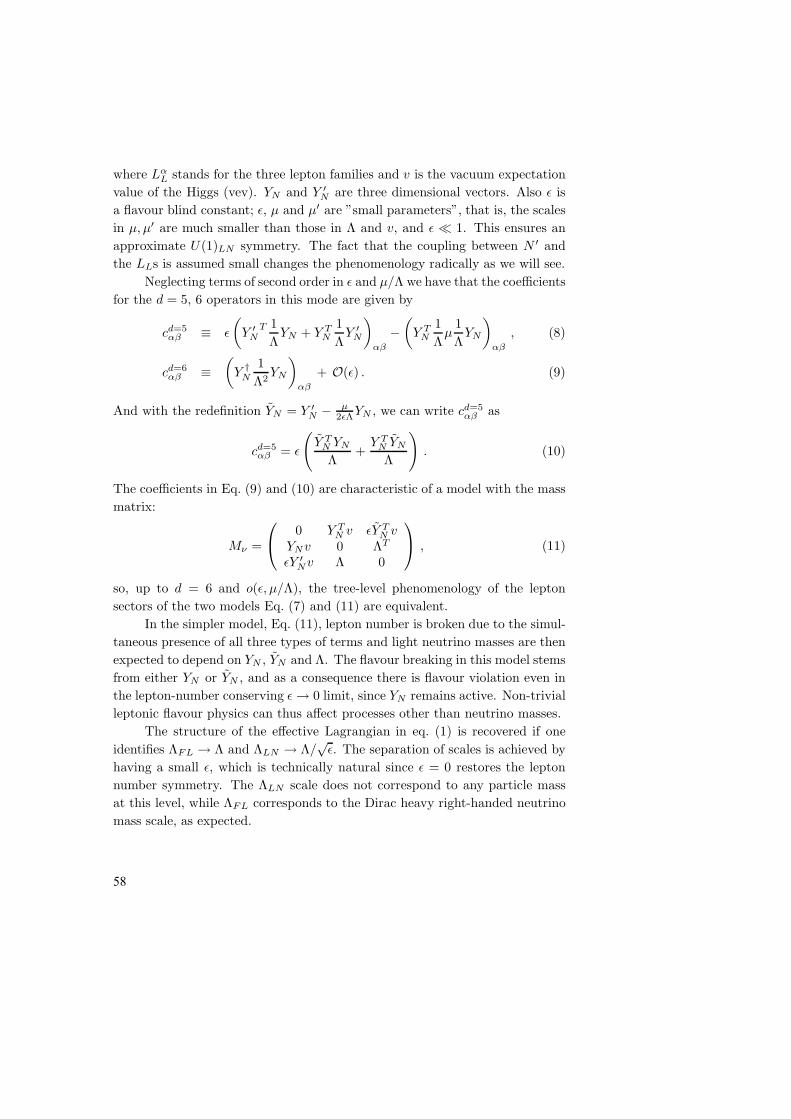
where LαL stands for the three lepton families and v is the vacuum expectation

value of the Higgs (vev). YN and Y ′

N are three dimensional vectors. Also ǫ is

a flavour blind constant; ǫ, µ and µ′ are ”small parameters”, that is, the scales

in µ, µ′ are much smaller than those in Λ and v, and ǫ ≪ 1. This ensures an

approximate U(1)LN symmetry. The fact that the coupling between N ′ and

the LLs is assumed small changes the phenomenology radically as we will see.

Neglecting terms of second order in ǫ and µ/Λ we have that the coefficients

for the d = 5, 6 operators in this mode are given by

cd=5αβ ≡ ǫ

(Y ′

N

T 1

ΛYN + Y T

N

1

ΛY ′

N

)

αβ

−

(Y T

N

1

Λµ

1

ΛYN

)

αβ

, (8)

cd=6αβ ≡

(Y †

N

1

Λ2YN

)

αβ

+ O(ǫ) . (9)

And with the redefinition YN = Y ′

N −µ

2ǫΛYN , we can write cd=5

αβ as

cd=5αβ = ǫ

(Y T

N YN

Λ+

Y TN YN

Λ

). (10)

The coefficients in Eq. (9) and (10) are characteristic of a model with the mass

matrix:

Mν =

0 Y T

N v ǫY TN v

YNv 0 ΛT

ǫY ′

Nv Λ 0

, (11)

so, up to d = 6 and o(ǫ, µ/Λ), the tree-level phenomenology of the lepton

sectors of the two models Eq. (7) and (11) are equivalent.

In the simpler model, Eq. (11), lepton number is broken due to the simul-

taneous presence of all three types of terms and light neutrino masses are then

expected to depend on YN , YN and Λ. The flavour breaking in this model stems

from either YN or YN , and as a consequence there is flavour violation even in

the lepton-number conserving ǫ → 0 limit, since YN remains active. Non-trivial

leptonic flavour physics can thus affect processes other than neutrino masses.

The structure of the effective Lagrangian in eq. (1) is recovered if one

identifies ΛFL → Λ and ΛLN → Λ/√

ǫ. The separation of scales is achieved by

having a small ǫ, which is technically natural since ǫ = 0 restores the lepton

number symmetry. The ΛLN scale does not correspond to any particle mass

at this level, while ΛFL corresponds to the Dirac heavy right-handed neutrino

mass scale, as expected.

58

As it turns out, the d = 5 coefficient in this case has also enough informa-

tion to reconstruct both Yukawa vectors up to a global renormalization, and

therefore, also the flavour structure of cd=6αβ

3). Let U be the PMNS matrix,

found by diagonalizing cd=5αβ , and let

Y TN ≡ yu Y T

N ≡ yv, (12)

where y and y are real numbers 〈u, u〉 = 〈v, v〉 = 1. Then, after choosing a

particular hierarchy, normal or inverted, the Yukawa couplings can be recon-

structed as linear combinations of the columns of the PMNS matrix. For the

normal (inverted) hierarchy we find 3)

YN i =y√

2

[f1(r) U∗

i3(i2) + f2(r) U∗

i2(i1)

], (13)

YNi=

y√

2

[f1(r) U∗

i3(i2) − f2(r) U∗

i2(i1)

]. (14)

where

r ≡|∆m2

solar|

|∆m2atmos|

=|∆m2

12|

|∆m223|

. (15)

and f1,2 are well determined functions 3). Moreover, since one neutrino

is massless, the absolute values of the masses can also be determined from

∆m2solar and ∆m2

atmos. Finally, using all low energy observables we can find

the value of the combination

ǫyy

Λ

∣∣∣ ∼ 4.9(8.1)× 10−13 TeV−1. (16)

From Eq. (13) we obtain the coefficient cd=6 and hence, predictions for the

rare decays. We show in Fig. 1 the result for the ratios Beµ/Beτ , Beµ/Bµτ ,

etc, as a function of θ13. One feature to be noted about these ratios for this

particular model is the strong dependence on the Majorana phase α as well as

on the CP phase for higher values of θ133).

4 Conclusions

In this work we identified an extremely simple model of neutrino masses that

requires only 2 heavy neutrinos. The Yukawa couplings of this model can

be determined in terms of the light neutrino mass matrix and, therefore, a

relation exists between the coefficient of the d = 5 Weinberg operatos and the

59

0.05 0.1 0.15 0.2 0.25s13

1

2

3

4

5

α=Π�4

α =0

0.05 0.1 0.15 0.2 0.25s13

0.20.40.60.8

11.21.4

α=Π�4

α =0

Figure 1: Ratio Beµ/Beτ for different values of the CP phase δ = 0 (solid) and

δ = π/2 (dashed), with α = 0, π/4 as denoted. Left: Normal hierarchy. Right:

Inverse hierarchy .

coefficients of the d = 6 operators involved in flavour processes. The flavour

violating rates induced by the d = 6 couplings can be reconstructed - including

CP phases - from the parameters in the light neutrino mass matrix.

In general, if new flavour physics in the lepton sector is to be accessible

and we stick to the Majorana paradigm of neutrino masses, then two scales

must be embedded in the fundamental theory ΛFL ≪ ΛLN . This should be

regarded as a guiding line for phenomenologically promising MFV models of

neutrino masses.

5 Acknowledgements

This work was made in collaboration with B. Gavela, T. Hambye and P. Her-

nandez. D. Hernandez has been partially supported by CICYT through the

project FPA2009-09017 and by MEC through FPU grant AP-2005-3603.

References

1. G. Isidori, Y. Nir and G. Perez, arXiv:1002.0900 [hep-ph].

2. V. Cirigliano, B. Grinstein, G. Isidori and M. B. Wise, Nucl. Phys. B 728

(2005) 121 [arXiv:hep-ph/0507001].

3. M. B. Gavela, T. Hambye, D. Hernandez and P. Hernandez, JHEP 0909

(2009) 038 [arXiv:0906.1461 [hep-ph]].

4. E. J. Chun, K. Y. Lee and S. C. Park, Phys. Lett. B 566 (2003) 142


60



NATURAL DIRAC NEUTRINOS FROM WARPED

EXTRA DIMENSION

Jackson M. S. WuAlbert Einstein Center for Fundamental Physics,

Institute for Theoretical Physics, University of Bern,Sidlerstrasse 5, 3012 Bern, Switzerland

Abstract

Dirac neutrinos arising from gauged discrete symmetry a la Krauss-Wilczekare implemented in the minimal custodial Randall-Sundrum model. In thecase of a normal hierarchy, all lepton masses and mixing pattern can be nat-urally reproduced at the TeV scale set by the electroweak constraints, whilesimultanously satisfy bounds from lepton flavour violation. A nonzero neutrinomixing angle, θ13, is generic in the scenario, as well as the existence of sub-TeVright-handed Kaluza-Klein neutrinos, which may be searched for at the LHC.

1 Introduction

Despite that the nature of neutrino remains unknown, most efforts has been

directed at Majorana neutrinos. One common reason cited against the Dirac

scenario is that it is hard to make realistic without excessive fine-tuning.

61

Recently, the Randall-Sundrum (RS) extra-dimensional scenario has be-

come a novel and powerful framework to understand flavour. The crucial fea-

ture is that the mass hierarchy of the Standard Model (SM) charged fermions

can arise naturally from their “geography” in the warped AdS5 bulk 1). The

Yukawa couplings need not be fine-tuned, and can be fully “anarchic” (i.e. all

naturally of order one and patternless). It was seen that the observed quark

mass and mixing pattern can be accurately reproduced in this approach 2), and

it is reasonable to expect the same can for Dirac neutrinos with appropriate

bulk localisations, which is indeed found to be the case 3).

2 The framework

The setting used is that of the Minimal Custodial RS (MCRS) model 4). The

bulk gauge group is SU(2)L × SU(2)R × U(1)B−L, which incorporates the

custodial symmetry protecting the ρ parameter. It is broken down to the SM

at the boundaries by the IR-localised SM Higgs, H1, and by UV boundary

conditions (BCs) and scalar vaccum expectation value (VEV).

Concentrating on the lepton sector, the leptons are embedded as

Li =

(νiL [+, +]eiL [+, +]

), Ei =

(νiR [−, +]eiR [+, +]

), νiR [+, +] , (1)

where i is a generation index, L, E denote SU(2)L,R doublets respectively,

and νR the right-handed (RH) neutrino singlet under SU(2)L,R. The parity

assignment + (−) denotes Neumann (Dirichlet) BCs applied to the spinors on

the boundary branes. Only fields with the [+,+] parity contain zero-modes

that are part of the low energy spectrum of the 4D effective theory after the

Kaluza-Klein (KK) reduction.

SM lepton masses arise as usual from Yukawa interactions with the SM

Higgs. To generate Dirac masses for the neutrinos, a second Higgs doublet,

H2, transforming only under the SU(2)L is introduced on the IR brane. After

electroweak symmetry breaking, the lepton mass matrices in the 4D effective

theory take the form

(MRSe,ν )ij =

vW

krcπλe,ν

5,ijf0L(π, ce,ν

iL )f0R(π, ce,ν

jR ) , (2)

where krcπ ≈ 37π is the warp factor solving the hierarchy problem, the Higgs

VEVs, v1 = v2 = vW = 174/√

2 GeV, are taken equal for simplicity, λe,ν5

62

are the complex dimensionless 5D Yukawa matrice for the charged leptons and

neutrinos, f0L,R are the zero-mode wavefunctions, and cL,R are the localisation

parameters (see 3) for more details).

3 Dirac neutrinos from a gauged discrete ZN

To have Dirac neutrinos, one needs to forbid Majorana mass terms, which can

be easily accomplished via a U(1) symmetry. Now if this U(1) is global, it

can be violated by quantum gravity effects. But if it is gauged, it has to be

broken to avoid any new massless gauge bosons appearing. However, a gauged

discrete ZN symmetry can survive from a gauged U(1) broken at some very

high scale 5), which is enough for Dirac neutrinos, as is well-known.

To implement this in the MCRS model, one extends the bulk gauge group

by a U(1)X , and add a scalar UV-localised, φ, charged under it:

Dµφ = (∂µ − ig5XXµ) φ , (3)

where Xµ is the U(1)X gauge field, and g5X the coupling constant. The U(1)X

is spontanously broken when φ acquires a VEV, vφ. Parametrising the scalar

as φ = (vφ + ρ)eiη/vφ , one sees that the Goldstone field, η, can be removed by

a gauge transformation and a concomitant fermion field redefinition:

Xµ → Xµ −1

g5X

∂µη

vφ

, f → f exp

(i

η

vφ

QX

). (4)

The ZN symmetry then emerges if QX , the fermion charge under the U(1)X ,

is rational but nonintegral.

4 Viability

To see if the Dirac neutrinos thus implemented can be realistic and natural, a

parameter space scan is performed searching for configurations that give rise to

the observed lepton mass (at a running scale of 1 TeV) and the bi-large mixing

pattern while satisfying the current lepton flavour bounds at the same time.

For the search, the KK scale is set to 3 TeV to satisfy electroweak pre-

cision test constraints. The 5D Yukawas are taken to be |λ5,ij | ∈ [0.5, 2.0] for

perturbativity. It is found that viable configurations compatible with all cur-

rent data and bounds arise only for the case of neutrino the normal hierarchy.

63

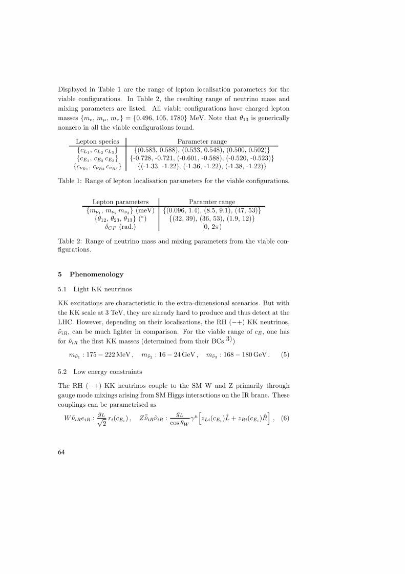
Displayed in Table 1 are the range of lepton localisation parameters for the

viable configurations. In Table 2, the resulting range of neutrino mass and

mixing parameters are listed. All viable configurations have charged lepton

masses {me, mµ, mτ} = {0.496, 105, 1780} MeV. Note that θ13 is generically

nonzero in all the viable configurations found.

Lepton species Parameter range{cL1

, cL2cL3

} {(0.583, 0.588), (0.533, 0.548), (0.500, 0.502)}{cE1

, cE2cE3

} {-0.728, -0.721, (-0.601, -0.588), (-0.520, -0.523)}{cνR1

, cνR2cνR3

} {(-1.33, -1.22), (-1.36, -1.22), (-1.38, -1.22)}

Table 1: Range of lepton localisation parameters for the viable configurations.

Lepton parameters Paramter range{mν1

, mν2mν3

} (meV) {(0.096, 1.4), (8.5, 9.1), (47, 53)}{θ12, θ23, θ13} (◦) {(32, 39), (36, 53), (1.9, 12)}

δCP (rad.) [0, 2π)

Table 2: Range of neutrino mass and mixing parameters from the viable con-figurations.

5 Phenomenology

5.1 Light KK neutrinos

KK excitations are characteristic in the extra-dimensional scenarios. But with

the KK scale at 3 TeV, they are already hard to produce and thus detect at the

LHC. However, depending on their localisations, the RH (−+) KK neutrinos,

νiR, can be much lighter in comparison. For the viable range of cE , one has

for νiR the first KK masses (determined from their BCs 3))

mν1: 175 − 222 MeV , mν2

: 16 − 24 GeV , mν3: 168 − 180 GeV . (5)

5.2 Low energy constraints

The RH (−+) KK neutrinos couple to the SM W and Z primarily through

gauge mode mixings arising from SM Higgs interactions on the IR brane. These

couplings can be parametrised as

WνiReiR :gL√

2ri(cEi

) , Z ¯νiRνiR :gL

cos θW

γµ[zLi(cEi

)L + zRi(cEi)R

], (6)

64

where gL ≡ e/ sin θW , θW the Weinberg angle, and L, R the usual chiral

projectors. The quantities ri, zLi and zRi involve gauge couplings and products

of wavefunction overlap integrals. For simplicity gL = gR is assumed.

With mν1> mπ, the charged kaon decay K+ → e+ν1 sets the most

stringent limit with the bound |r1|2 < 10−6 for a 160 to 220 MeV neutrino 6).

Another limit comes from the LEP invisible Z decay measurement, which gives

Nν = Γinv/ΓSMν = 2.9840 ± 0.0082 7). Since only ν1 is light enough to escape

the detector without leaving tracks, this sets a bound on Γ(Z → ¯ν1ν1) and

thus z2L1

+ z2R1

≤ 0.096 (95%CL). For the viable range of cE , these constraints

turns out to be very weak, as r1 ∼ O(10−6), while zL1 ∼ zR1 ∼ O(10−2).

5.3 Decay modes and LHC production

The decay modes of the RH (−+) KK neutrinos depends crucially on their

masses. For the heaviest O(100) GeV ν3, a decay predominantly into τ W is

expected with a width Γν3∼ 1.5 × 10−6 GeV for the viable range of cE .

For the (much) lighter ν1,2, three body decays are dominant. For ν1,

the dominant decay channel is the charged current (CC) decay ν1 → ee+νe1

with a width ΓCC1 ∼ 0.73 × 10−17|r1|

2 GeV, corresponding to a lifetime of

τν1∼ 2.3×104 s for the viable range of cE . For ν2, the main decays channels are

ν2 → µlνl, µud, µcs. The total width is estimated to be ΓCC2 ∼ 0.027|r2|

2 GeV,

and so a lifetime τν2∼ 1.2 × 10−15 s for the viable range of cE .

At the LHC, due to the large background ν1 is not expected to be

seen given that mν1≪ 1 GeV. For ν2, it can be detected via the process

ud → ν2µ+ → µ+µ−e(τ)ν. The final state will involve apparent lepton flavor

violation plus missing energy with the µ+µ− pair not in resonance, character-

istic of heavy neutrino signatures. Similarly, ν3 can be detected via the process

ud → τ+ν3 → τ+τ−W , where a W jet plus τ jets are expected with the τ jets

not in resonance. For the viable range of cE , the total production cross section

at√

s = 14 TeV is estimated to be ∼ 0.3 fb and ∼ 10−3 fb for ν2,3 respectively.

1The ν1 → eµ+νµ contribution is phase space suppressed, the e π mode isnegligible, while the virtual Z mediated amplitudes are unimportant.

65

6 Conclusion

It is shown that Dirac neutrinos can be naturally implemented in the MCRS

setting with a SU(2)L × SU(2)R × U(1)B−L × U(1)X bulk gauge symmetry

group a la Krauss-Wilczek. For normal neutrino hierarchy only, lepton masses

and mixing patterns can be successfully reproduced with just the RS anarchic

5D flavour structure, at the TeV scale, and at the same time still satisfy the

lepton flavour bounds.

In the Dirac neutrino scenario presented, θ13 is generially neither zero nor

small, which can be tested at the upcoming long-baseline experiments. There

are also light KK neutrinos in the spectrum, of which the O(200) MeV ν1 is too

light to be picked out at the LHC but has a long life time of O(104) s, the heavy

O(200) GeV ν3 has to small a production rate, leaving only the O(20) GeV ν2

possible to be searched for at the LHC.

7 Acknowledgements

JW thank LNF for the hospitality and support provided during the 2nd Young

Researchers Workshop.

References

1. N. Arkani-Hamed and M. Schmaltz, Phys. Rev. D 61, 033005 (2000),

Y. Grossman and M. Neubert, Phys. Lett. B 474, 361 (2000).

2. W. F. Chang, J. N. Ng and J. M. S. Wu, Phys. Rev. D 78, 096003 (2008);

79, 056007 (2009).

3. W. F. Chang, J. N. Ng and J. M. S. Wu, Phys. Rev. D 80, 113013 (2009).

4. K. Agashe, A. Degado, M. J. May and R. Sundrum, JHEP 0308, 050

(2003).

5. L. M. Krauss and F. Wilczek, Phys. Rev. Lett. 62, 1221 (1989).

6. C. Amsler et al., Phys. Lett. B 667 (2008) 1.

7. ALEPH Collaboration et al., Phys. Rept. 427, 257 (2006).

66



FLAVOUR IN SOFT LEPTOGENESIS∗

Chee Sheng FongC. N. Yang Institute for Theoretical Physics, Stony Brook University

Abstract

Successful Soft Leptogenesis (SL) requires a relatively low mass scale for theSU(2) singlet neutrinos of 105 − 108 GeV. However, conventional SL (un-flavoured) requires an unnaturally small soft supersymmetry(SUSY)-breakingbilinear B ≪ O(TeV) coupling for successful leptogenesis. On the other hand,in this regime, the interactions mediated by τ , µ (and even e) charged leptonYukawa interactions are in equilibrium, making the lepton number asymme-tries and the washouts flavour dependent. Hence, it is crucial to take intoaccount the flavour effects. Considering a general soft SUSY-breaking trilinearA couplings, it is possible to enhance the efficiency up to O(1000) comparedto the unflavoured case. With the enhanced efficiency, we can raise the B upto TeV scale for successful leptogenesis. Taking into account the low energyconstraints, we verify that the fast lepton flavour violation processes inducedby the soft SUSY-breaking slepton masses would not destroy the enhancement.

∗Work done in collaboration with M. C. Gonzalez-Garcia, Enrico Nardiand Juan Racker. Based on hep-ph/1004.5125.

67

1 Soft Leptogenesis Lagrangian and CP Asymmetries

The type-I SUSY seesaw model can be described by the superpotential:

W = WMSSM +1

2MijNiNj + YikǫαβNiL

αk Hβ , (1)

where WMSSM is the superpotential for the Minimal Supersymmetric Standard

Model (MSSM), k = 1, 2, 3 are the lepton flavour indices, Mij are the Majorana

masses of the right-handed singlet neutrinos with generation indices i, j, and

Ni, Lk, H are the chiral superfields for the right-handed singlet neutrinos,

the left-handed lepton doublets and the Higgs doublets, with ǫαβ = −ǫβα and

ǫ12 = +1.

The relevant soft SUSY-breaking terms are given by

−Lsoft = AZikǫαβNiℓαkhβ +

1

2BijMijNiNj + meℓkl

ℓk ℓl + h.c. (2)

The singlet sneutrino and anti-sneutrino states mix, giving rise to the

mass eigenstates:

N+i =1√

2(eiΦ/2Ni + e−iΦ/2N∗

i ),

N−i =−i√

2(eiΦ/2Ni − e−iΦ/2N∗

i ), (3)

where Φ ≡ arg(BM), that correspond to the mass eigenvalues

M2ii± = M2

ii ± |BiiMii|. (4)

For simplicity, we will concentrate on SL arising from a single sneutrino

generation i = 1 and in what follows we will drop that index. After superfield

phase rotations, we have three independent physical phases, they are

φAk = arg(ZkY ∗

k AB∗), (k = 1, 2, 3) (5)

Eq. (2) leads to CP asymmetries ǫk(T ) arising from self-energy diagrams

induced by the bilinear B term,

ǫk (T ) = −Pk

Zk

Yk

sinφAk

A

M

4BΓ

4B2 + Γ2∆BF (T ) , Pk ≡

Y 2k∑

j

Y 2j

, (6)

68

where

∆BF (T ) =cs(T ) − cf (T )

cs(T ) + cf (T ), (7)

is the thermal factor associated to the difference between the phase-space, Bose-

enhancement and Fermi-blocking factors for the scalar and fermionic channels,

that vanishes in the zero temperature limit ∆BF (T =0) = 0 2, 3).

2 Flavour Structure

Regarding the flavour structure of the soft terms relevant for flavoured SL, we

can distinguish two general possibilities:

1. Universal soft SUSY-breaking terms. This case is realized in supergrav-

ity and gauge mediated SUSY-breaking models (neglecting the renormalization

group running of the parameters), in our notations corresponds to

Zk = Yk. (8)

In this case the only flavour structure arises from the Yukawa couplings and

both the CP asymmetries ǫk and the corresponding washout terms are pro-

portional to the same Pk, resulting in mild enhancement of O(30) in efficiency

from one-flavour approximation 4). We refer to this case as Universal Trilinear

Scenario (UTS).

2. General soft SUSY-breaking terms. The most general form for the

soft-SUSY breaking terms is allowed, only subject to the phenomenological

constraints from limits on flavour changing neutral currents (FCNC) and from

lepton flavour violating (LFV) processes. To simplify the analysis while still

capture some of the main features of the general case, we choose

Zk =

∑

j

|Yj |2

3Y ∗

k

, (9)

such that the CP asymmetries become flavour independent, ǫk = ǫ/3 for each

flavour. In what follows we will refer to this case as the Simplified Misaligned

Scenario (SMS). With this choice, since it is possible to reduce the washout in

a particular flavour direction while keeping the corresponding CP asymmetry

fixed, a much greater enhancement than the UTS becomes possible.

In both the UTS and SMS, from (5), we see that we only have one unique

phase φA = arg(AB∗).

69

3 Results

We numerically solved the relevant Boltzmann Equations 1 to obtain the final

amount of B − L asymmetry generated in the decay of the singlet sneutrinos

(assuming no pre-existing asymmetry) which can be parametrized as:

YB−L(z → ∞) = −2η ǫ Y eq

eN(T ≫ M), η ≡

∑

k

ηk. (10)

After conversion by the sphaleron transitions, the final baryon asymmetry

is related to the B − L asymmetry by

YB =8

23YB−L(z → ∞). (11)

We also define the N± decay parameter, meff ≡∑

k Y 2k v2

u/M which is

related to the washout parameter K as K = Γ eN/H(M) = meff/m∗ where Γ eN

is the total singlet sneutrino decay width, vu = v sin β (with v = 174 GeV),

m∗ =√

πg∗

45×

8π2v2

u

mP

∼ 10−3 eV with g∗s the total number of relativistic degrees

of freedom (g∗ = 228.75 in the MSSM) and mP the Planck mass.

In the left panel of Fig. (1), we plot the efficiencies as a function of meff for

both the scenarios UTS and SMS. Deviating from the flavour equipartition case

P1 = P2 = P3 = 1/3, in the SMS, we can obtain an enhancement up to O(1000)

compared to the one-flavoured approximation. With this enhancement, it is

possible to push the values of B up to natural values at TeV scale for successful

leptogenesis as shown in the right panel of Fig. (1).

unflavoured

∑ kη

k

meff(eV)

P3=

0.99,SM

S

P3=

1/3,U

TS/SM

S

P1 = P2P3 = 0.99, UTS

, SMS

, SMS

, UTS

, UTS

Bm

ax

P3

1−P

3

P3

1 − P3

P1 = P2

Figure 1: Left: The dependence of the efficiencies on meff . Right: Maximumvalues of B which can lead to successful leptogenesis as a function of P3 and1 − P3. The figures correspond to A sin φA=1 TeV and tanβ = 30.

1For more details, please refer to Ref. 1)

70

4 Low Energy Constraints

As has been highlighted in Ref. 5), at sufficiently low temperatures the off-

diagonal soft-SUSY breaking slepton masses can give rise to lepton flavour

equilibration (LFE), effectively damping all dynamical flavour effects. In the

left panel of Fig. (2), we show the dependence of the efficiencies (normalized to

the flavour equipartition case) on the off-diagonal soft slepton mass parameter

mod which for simplicity, we assume to be flavour independent. We see that

there is a cut-off value of mod for each M such that the enhancement is totally

damped out. In the right panel of Fig. (2), we show that in most part of

the SUSY parameter space that is relevant for SL, subjecting to low energy

constraints, the large flavour enhancements can survive the LFE effects.

GeV

GeV

∣ ∣ ∣ ∣η/η

1/3

∣ ∣ ∣ ∣

mod (GeV)

M=

105

M=

106

P = (0.005, 0.005, 0.99)

meff = 0.1eV

m∼od

/ GeV

MSUSY/TeV

Figure 2: Left: The dependence of the efficiencies (normalized to the flavourequipartition case) on the off-diagonal soft slepton mass parameter mod. Right:Excluded region (shaded in yellow) of mod versus mSUSY arising from thepresent bound of BR(µ → eγ) ≤ 1.2 × 10−11, together with the minimumvalue of mod for which LFE effects start damping out flavour effects. Threelines shown corresponds to M = 105 GeV, M = 106 GeV and M = 107 GeV.The vertical dashed line represents the value of mSUSY/(30)

1

2 required to ex-plain the discrepancy between the Standard Model (SM) prediction and the

measured value of muon anomalous magectic moment aµ6). In the plots, we

assume tanβ = 30.

5 Acknowledgements

The speaker thanks Concha Gonzalez-Garcia, Enrico Nardi and Juan Racker

with whom he collaborated with in this work. He is also grateful to the 2nd

71

Young Researchers Workshop (in conjuction with XV Frascati Spring School

“Bruno Touschek”) organizing committee for the hospitality during his stay in

beautiful Frascati.

References

1. C. S. Fong, M. C. Gonzalez-Garcia, Enrico Nardi, and J. Racker, To appear

[arXiv:1004.5125 [hep-ph]].

2. Y. Grossman, T. Kashti, Y. Nir and E. Roulet, Phys. Rev. Lett. 91 (2003)

251801 [arXiv:hep-ph/0307081].

3. G. D’Ambrosio, G. F. Giudice and M. Raidal, Phys. Lett. B 575, 75 (2003)


4. C. S. Fong and M. C. Gonzalez-Garcia, JHEP 0806 (2008) 076

[arXiv:0804.4471 [hep-ph]].

5. D. Aristizabal Sierra, M. Losada and E. Nardi, JCAP 0912, 015 (2009)

[arXiv:0905.0662 [hep-ph]].

6. S. Davidson, J. Garayoa, F. Palorini and N. Rius, JHEP 0809, 053 (2008)

[arXiv:0806.2832 [hep-ph]].

72



MODEL INDEPENDENT AND GENUINE FIRST

OBSERVATION OF TIME REVERSAL VIOLATION

Jose BernabeuDepartment of Theoretical Physics, University of Valencia

IFIC Joint Center Univ.Valencia-CSIC

TH Unit, CERN, Geneva

Fernando Martınez-VidalIFIC (Valencia University)

Pablo Villanueva-PerezIFIC (Valencia University)

Abstract

This document discusses the proposal and feasibility studies to perform for thefirst time a separate and independent experimental test of Tviolation usingB-factory data.

1 Theoretical Motivation

The violation of CP invariance has been observed in the K0− K0 and B0− B0

systems. Up to now, the experimental results are in agreement with the

Cabibbo-Cobayashi-Maskawa (CKM) mechanism. On the other hand, CPT

invariance imposed by any local quantum field theory with Lorentz invariance,

is confirmed by all avaliable data. A direct evidence for time-reversal violation

(TRV) in a single experiment, independent of CP violation and CPT invari-

ance, would be of great interest. There is no existing result 1) that clearly

73

demonstrates TRV in this sense. Sometimes the Kabir asymmetry K0 → K0

vs. K0 → K0 has been presented 2) as a proof for TRV. This process has,

however, besides the drawbacks discussed in 1), the feature that K0 → K0

is a CPT-even transition, so that it is impossible to separate T violation from

CP violation.

There are effects in particle physics that are odd under time t, but they

are not genuine T-violating, because do not correspond to an interchange of

”in” into ”out” states. In fact, the t-asymmetry can only be connected 4) to

T-asymmetry under the assumptions of CPT invariance plus the absence of an

absorptive part difference between the initial and final states of the transition.

As a consequence, we have to disregard these t-asymmetries as direct evidence

for T violation.

As shown in Refs. 4, 5), B-factories offer a unique opportunity to show

separate evidence for T violation (and CP violation) and measure the corre-

sponding effects. The proposal has been scrutinized by Lincoln Wolfenstein 1)

and Helen Quinn 3) with the conclusion that it appears to be a true TRV-

effect. The crucial role played by B-factories is the EPR entanglement 6)

between the neutral B-mesons produced by the Υ(4S) decay.

Although this coherence imposed by Bose statistics has only been used

for flavor tagging up to now, one has to emphasize, following what quantum

mechanics dictates, that the individual state of the neutral meson is not defined

before its collapse as a filter imposed by the observation of the decay process of

its companion. Similarly to the writing of the physical state of the two particles

in terms of Bose-correlated orthogonal B0 and B0, which allows to infer the

flavor of the still alive meson by observing the specific flavor decay of the other

(and first decaying) meson, one can rewrite the two particle state in terms of

any pair of orthogonal states of individual neutral B-mesons. In particular, let

us consider the pair of orthogonal states B+ andB− of neutral B-mesons, where

B− is the state that decays to J/ψK+, K+ being the neutral K+ → ππ, and

B+ is the orthogonal state to B−, i.e., not connected to J/ψK+. We may call

the filter imposed by a first observation of one of these decays a “CP-tag” 6),

because B+ and B− are approximately, up to terms of Re(ǫK) giving the non-

orthogonality of KL and KS , the neutral B-mesons associated with final states

of their decays which are CP-eigenstates, with the identification of K+ ≡ KS.

As we are going to discuss much larger expected effects, one is authorized to

74

use the language of identifying B− by J/ψKS , and B+ by J/ψKL. To clarify

the point, B− and B+ should not be associated with CP-eigenstates of the

neutral B mesons themselves.

The theoretical ingredient to be used for this proposal is the EPR en-

tanglement. Let us consider the two particle state of the neutral B-mesons

produced by the Υ(4S) decay:

|i >=1√

2[B0(t1)B

0(t2)− B0(t1)B

0(t2)] =1√

2[B+(t1)B−(t2)−B−(t1)B+(t2)],

(1)

where the states 1 and 2 are defined by the time of their decay with t1 < t2. We

may proceed to a partition of the complete set of events into four categories,

defined by the tag in the first decay as B+ , B− , B0 or B0. Let us take as

process I B0 → B+, through the observation of a negatively charged lepton

l− first (produced by the semileptonic decay of the opposite B0 meson) and

J/ψKL later, denoted as (l−,J/ψKL), and consider:

• I.i) Its CP transformed B0 → B+ (l+,J/ψKL), so that B0 → B+ and

B0 → B+, as a function of ∆t = t2 − t1, provide a genuine CP-violating

asymmetry.

• I.ii) Its T transformed B+ → B0 (J/ψKS, l+), so that B0 → B+ and

B+ → B0, as a function of ∆t = t2 − t1, provide a genuine T-violating

asymmetry.

• I.iii) Its CPT transformed B+ → B0 (J/ψKS , l−), so that B0 → B+and

B+ → B0, as a function of ∆ = t2 − t1, provide a genuine CPT-violating

asymmetry.

One may check, a fortiori, that the events used for the asymmetries I.i),

I.ii) and I.iii) are completely independent. Furthermore, the expectation is

that the asymmetry described by I.ii) will prove and measure, for the first

time, T violation with a large significance. Similarly, one may take as reference

processes II (B0 → B−), III (B0 → B+) and IV (B0 → B−).

On purpose, up to now there is no reference to the results expected for

all these genuine asymmetries in the Weisskopf-Wigner effective Hamiltonian

approach for the time evolution of the B0 − B0 system, as well as within the

standard CKM mechanism for CP violation 4, 5). We proceed in this way

75

since our goal is to demonstrate and measure the violation of time reversal

invariance without using the procedure of fitting parameters in a given theory.

The outcome will be a model-independent observation of T violation.

2 Monte Carlo Study

In this section we describe the procedure we have followed to generate the

simulated samples of the required decays, as discussed previously. In the second

part, we estimate the T violation asymmetry and its expected significance with

the size of currently available B-factory data samples.

Concerning to the Monte Carlo simulation, it has been done using an

standard probability density function (PDF) which contains effects of T, CP

and CPT violation and is based on the Wigner-Weiskopff formalism 8). Ne-

glecting effects from mistags, CPT violation (complex parameter z set to zero),

and taking ∆Γ = 0, |q/p| = 1, the decay rate g± from a neutral B meson to a

CP eigenstate (B+, B−) is given by equation 2 taken from 8, 9) 8, 7). To

generate our samples we have set the parameter Im(λf ) (i.e. the well known

CP-violating parameters sin 2β) to 0.672 and |λf | = 1, so Sf = 0.672 and

Cf = 0 (i.e. no direct CP violation in the B+, B− decays), taken from 9):

g±(∆t) =e

−|∆t|

τB0

4τB0

{1 ± [Sfsin(∆md∆t) − Cf cos(∆md∆t)]} (2)

With this PDF we generate the eight subsamples, from which we evaluate

our asymmetries.

The T asymmetry (AT (∆t)) is built counting the number of entries in

each generated subsample (Na) and its T transformed (Nb). Then we subtract

bin by bin in ∆t the entries from the two subsamples, correcting by efficiency

effects. Taking as example the BaBar experiment, we consider 3255 J/ψKL and

7750 J/ψKS signal events, obtaining the data points in the T asymmetry plots

(figure 1). The red dotted curves are obtained after setting Im(λCP ) = 0, which

in practice correspond to the integration over the bin size of the curve without

T violation. These curves have been produced generating 1 million events (i.e.

a virtually infinite statistics). We perform this comparison since our final goal

is to compare the asymmetries with T violation and the corresponding ones

without T violation with all the experimental effects included. This comparison

will be done through a χ2 test.

76

t (ps)∆0 2 4 6 8 10 12 14 16 18 20

TA

-1

-0.5

0

0.5+ B→ 0B

t (ps)∆0 2 4 6 8 10 12 14 16 18 20

TA

-0.5

0

0.5

1 - B→ 0B

t (ps)∆0 2 4 6 8 10 12 14 16 18 20

TA

-1

-0.5

0

0.5

+ B→ 0

B

t (ps)∆0 2 4 6 8 10 12 14 16 18 20

TA

-1

-0.5

0

0.5

- B→ 0

B

Figure 1: T asymmetries for each reference process with proper-time resolu-

tion, mistags, efficiency effects (black dots) and curves without T violation

(red dashed curves)

In our exercise we have included approximate ∆t resolution, mistags and

reconstruction efficiencies as observed at the B factories.

Finally, we perform a χ2 test for each of the four statistically independent

T asymmetries, using the χ2 ansatz given by

χ20 =

∑

∆ti

(AexpT (∆ti) − ANoT−V iolation

T (∆ti))2

σ2

Aexp

T

(∆ti) + σ2

ANoT−V iolation

T

(∆ti), (3)

from which a confidence level (or equivalently a significance of the T violation

effect) can be computed. For this study we assume a χ2-distributed variable,

although in the experimental analysis a careful study of the true distribution

will have to be pursued.

Assuming a χ2 distribution, the results of the χ2 test for T asymmetry

with proper-time resolution, mistags, and efficiency effects for our simulated

samples are summarized in Table 1. We can compute that χ2/dof ≈ 14 for

the TRV test, so we can anticipate to establish directly for the first time T

violation with a significance above 10 standard deviations.

77

Table 1: χ2 test of the T asymmetries.

T asymmetries Test B0→ B+ B0

→ B−

B0→ B+ B0

→ B−

χ2

0326.7, 21 bins 361.0, 21 bins 327.9, 22 bins 278.8, 22 bins

Prob(χ2 > χ2

0) 1.12 · 10−56 1.04 · 10−63 2.55 · 10−56 2.32 · 10−46

3 Acknowledgments

This research has been supported in part by the MICINN, Grant FPA 2008-

02878 and the Generatitat Valenciana Grant PROMETEO 2008/004.

References

1. L. Wolfenstein, Int. J. Mod. Phys. E 8, 501 (1999).

2. T. Nakada, Discrete’08 Conference, Valencia 2008, J. Phys. Conf. Ser. 171,

011001 (2009).

3. H. R. Quinn, Discrete’08 Conference, Valencia 2008, J. Phys. Conf. Ser.

171, 011001 (2009).

4. M. C. Banuls and J. Bernabeu, Phys. Lett. B 464, 117 (1999), [arXiv:hep-

ph/9908353].

5. M. C. Banuls, J. Bernabeu, Nucl. Phys. B 590, 19 (2000), [arXiv:hep-

ph/0005323].

6. M. C. Banuls, J. Bernabeu, JHEP 032, 9906 (1999), [arXiv:hep-

ph/9807430].

7. B. Aubert et al. (BaBar Collaboration), Phys. Rev. D 66, 032003 (2002);

K. Abe et al. (Belle Collaboration), Phys. Rev. D 66, 032007 (2002).

8. B. Aubert et al. (BaBar Collaboration), Phys. Rev. Lett. 92, 181801 (2004);

Phys. Rev. D 70, 012007 (2004).

9. B. Aubert et al. (BaBar Collaboration), Phys. Rev. D 79, 072009 (2009);

K.F. Chen et al. (Belle Collaboration), Phys. Rev. Lett. 98, 031802 (2007).

78



MEASURING sin φs FROM NEW PHYSICS

POLLUTED B DECAYS

Marc RamonUnitat de Fısica Teorica, Universitat Autonoma de Barcelona

Edifici Cn., 08193 Bellaterra (Barcelona), Spain.

Abstract

We discuss an alternative approach to measure the weak mixing angle φs of theB0s − B0

s system, using a theoretical input which is short-distance dominated inQCD factorisation and thus free of IR-divergencies at O(αs). We also present anew expression that allow to obtain directly sinφNPs if there is only a significantcontribution of New Physics in the mixing.

1 Introduction

An intensive research has been performed on the phenomenology of hadronic Bd

decays for the past 20 years, mainly at the B-factories BaBar and Belle working

around the Υ ressonance. The analysis of the data collected has proven that

the CKM mechanism is accurate enough to describe most of CP and flavour

violation phenomena observed in the energy range explored so far. Only the D0

79

and CDF experiments at Fermilab have been able to make some measurements

on the Bs system, namely the mass difference ∆Ms, other mixing parameters

and some decay modes. However, this situation is going to change with the

starting of LHCb, the upgrade of Belle and the future building of a Super-B

factory, so the list of observables measured for Bs decays will grow to constitute

a good place to look for New Physics (NP).

From a theoretical point of view, the study of non-leptonic B-decays

is rather involved, due to the presence of important long-distance strong in-

teraction effects. Having them under control is crucial to be able to resolve

small NP contributions. Two methods have been used in the literature to han-

dle these low-energy effects: flavour symmetries and direct computations from

QCD. Flavour symmetries suffer from big uncertainties, mainly due to poorly

estimated SU(3) breaking, while the direct computations from QCD, appear-

ing for instance in QCD factorisation (QCDf), are based on factorisation and

the 1/mb expansion, and may suffer from uncertainties due to non-factorisable

chirally enhanced 1/mb corrections and long distance charm loops.

2 Theoretical inputs from QCDf

2.1 The amplitudes

If there is no NP entering the amplitude, the unitarity of the CKM matrix

λ∗(s)u + λ∗(s)

c + λ∗(s)t = 0, (1)

allows us to write the amplitude of a B meson decaying into two light mesons

as

A(Bs → M1M2) = λ∗(s)u T

(s)

M1M2+ λ∗(s)

c P(s)

M1M2, (2)

where λ(s)q = V ∗

qsVqb. Using QCDf for B → PP decays, the amplitudes can be

rewritten as

A(Bs → M1M2) = AM1M2f1(a

(p)i ) + BM1M2

f2(bj), (3)

where p = u, c quarks, f1 (f2) denotes a linear combination of a(p)i (bj) and

a(p)i =

(Ci +

Ci±1

NC

)Ni(M2) +

Ci±1

NC

CFαs4π

[Vi(M2) +

4π2

NC

Hi(M1, M2)

]

+P(p)i (M2), (4)

bj ∝ f3(CjΦj ⊗ Tj). (5)

80

Eq. 3 gives the structure of the amplitude in QCDf, while the exact expressions

can be found in 1). Ci,j are the Wilson coefficients of the effective Hamiltonian

associated to these processes. The meson functions appearing in a(p)

i corre-

spond, respectively, to the single leading order diagram (Ni(M2)), to the four

hard-vertex correction diagrams (Vi(M2)), to the two hard-spectator scatter-

ing (HSS) diagrams (Hi(M1, M2)) and to the two penguin diagrams (P(p)i (M2))

appearing in the B decays into light mesons. The bj terms, are given by linear

combinations of light-cone distribution amplitudes (Φj) convoluted with hard-

scattering kernels (Tj), and are related to the four weak annihilation (WA)

diagrams.

2.2 The divergencies

The HSS terms are proportional to 1)

Hi(M1M2) ∝AM1M2

BM1M2

∫ 1

0

dx

∫ 1

0

dy

[ΦM2

(x)ΦM1(y)

xy+ rM1

χ

ΦM2(x)Φm1

(y)

xy

],

(6)

where x and y are the quark momentum fractions inside the mesons and rM1χ ∼

ΛQCD/mb. The y part of the second term in eq. 6 can be expressed 1)

∫ 1

0

dy

yΦm1

(y) = Φm1(1)

∫ 1

0

dy

y+

∫ 1

0

dy

y[Φm1

(y) − Φm1(1)] (7)

and, since the first integral is divergent as y → 0, an IR-divergence arises in

Hi(M1, M2); the same kind of divergent integrals come from the WA contri-

butions around the regions x, y ∼ 1. Each divergent contribution have been

parametrised in the literature 1) introducing a model-dependent parameter

XMl

k = (1 + ρkeiψl)ln(mb/ΛQCD), where k = H, A accounts for the origin of

the divergency (HSS or WA) and l for the final-state meson involved.

3 Construction of a theoretically clean input

3.1 A nice example: the decay B → K0K0

The T and P contributions for this exclusive process can be computed in QCDf,

obtaining 1)

T 0s = AKK [α

(u)

4 − (1/2)α(u)

4,EW + β3 + 2β4 − (1/2)β3,EW − β4,EW ], (8)

P 0s = AKK [α

(c)4 − (1/2)α

(c)

4,EW + β3 + 2β4 − (1/2)β3,EW − β4,EW ], (9)

81

with α(p)4 = a

(p)4 + rM2

χ a(p)6 and βk ∝ bk. It is straightforward to see that in the

quantity ∆ ≡ T −P 2), all β terms cancel and, with them, the IR-divergencies

coming from the weak annhilition terms. As the only term in eq. 4 that

actually depends on the final up-type quark (u or c) is P(p)i (M2), which can be

computed perturbatively, we get (neglecting the EW penguins)

∆ = T 0s − P 0

s ≃

[P

(u)

4 (K0) − P(c)4 (K0)

]+ rK

0

χ

[P

(u)

6 (K0) − P(c)6 (K0)

], (10)

so we have also gotten rid of the IR-divergencies coming from the HSS terms.

Thus, in some kinds of penguin mediated decays ∆ is free from IR-

divergencies at O(αs) in QCDf. This will lead to smaller uncertainties and

safer predictions than the full amplitude computed directly using QCDf.

3.2 The vectorial partner: Bs → K∗0K∗0

The magnitude ∆ has been derived for B → PP , but can also be applied

to the longitudinal component of the polarisation of final vector mesons in

B → V V decays. The advantages of doing so are the following: (1) larger

branching ratios, Br(Bs → K∗0K∗0) ∼ O(10−6), make them easier to measure

in hadronic machines; (2) the final decay products are charged (K∗0 → K+π−

and K∗0 → K−π+) and thus easier to identify, and have CP -eigenstates in

the final state; (3) the longitudinal observables are better behaved (H0 is not

suppressed, while H− is suppressed by 1/mb and H+ by 1/m2b

3)).

4 The sum rule

4.1 The building blocks

The longitudinal CP -asymmetries can be defined as 2, 4)

Alongdir ≡

|A0|2 − |A0|

2

|A0|2 + |A0|

2, A

longmix ≡ −2ηf

Im(e−iφsA∗

0A0

)

|A0|2 + |A0|

2,

Along∆Γ

≡ −2ηfRe

(e−iφsA∗

0A0

)

|A0|2 + |A0|

2, (11)

fulfilling |Alongdir |2 + |A

longmix |

2 + |Along∆Γ

|2 = 1, and the CP -averaged longitudinal

branching ratio

Brlong =< Γlongi >

CP∑i Γi

= τBΓlongB0

→f+ Γlong

B0→f

2= gPS

|A0|2 + |A0|

2

2. (12)

82

where A0 labels the longitudinally polarised V amplitude, ηf = ±1 is the

CP -eigenvalue of the final state f and gPS contains the phase-space factors.

From now on the superscript “long” will be dropped to simplify the notation,

although we will keep dealing with longitudinal observables.

4.2 Derivation of the sum rule

From the longitudinal component of eq. 2 and its CP -conjugated partner it

can be found

∆s =(λ

(s)u + λ

(s)c )A0 − (λ

∗(s)u + λ

∗(s)c )A0

λ∗(s)u λ

(s)c − λ

(s)u λ

∗(s)c

. (13)

Taking its modulus squared and substituting the building blocks (eqs. 11 and

12), it can be obtained 2)

|∆s|2 =

2Br

gPS

{x1 + [x2 sinφs − x3 cosφs]

Amix

ηf− [x2 cosφs + x3 sinφs]

A∆Γ

ηf

},

(14)

here x1, x2 and x3 are functions of just |λ(s)u |, |λ

(s)c | and γ.

5 Consistency test of the Standard Model

In the SM, eq. 1 can be rearranged into (|λ(s)u |/|λ

(s)c |)eiγ−(|λ

(s)t |/|λ

(s)c |)e−iβ

SM

s =

−1 and the B0s − B0

s mixing angle φSMs = 2βSMs +O(λ6). These two conditions

make x2 sin φs − x3 cosφs = 0, which cancels the second term in eq. 14.

Now, transforming |∆s|2 conveniently one can get 4)

sin(βSMs ) =Br/gPS

2|λ(s)c |2|∆s|

2

[1 −

1

ηf

√1 − (Adir)2 − (Amix)2

]. (15)

This is a consistency test of the SM : measuring the Br, Adir and Amix and

computing |∆s|, the value of βSMs can be predicted. Therefore, if a value of βs

incompatible with βSMs is measured, it would constitute a signal of NP. Alter-

natively, and since A∆Γ =√

1 − (Adir)2 − (Amix)2, if A∆Γ can be determined

experimentally, the Br will be the only other observable needed to extract βs.

This can be done measuring the time-dependent longitudinal untagged rate

Γ(Bs(t) → V V ) + Γ(Bs(t) → V V ) ∝ RHe−ΓH

st + RLe−Γ

L

st, from where A∆Γ

can be obtained:

A∆Γ(Bs → V V ) =RH − RL

RH + RL

. (16)

83

6 Extraction of sin φs in presence of New Physics in the mixing

If NP enters only the B0s − B0

s mixing, then φs = 2βSMs + φNPs , and the sum

rule can be written as

sin φNPs =1

ηf

Amix(1 − C) − sign(Amix)|A∆Γ|√

1 − (Adir)2 − (1 − C)2

1 − (Adir)2, (17)

where C ≡ 2|λ(s)c |2 sin2 βSMs gPS |∆|2/Br and, given that NP enters only via the

mixing angle, Adir = ASMdir . The interpretation of eq. 17 is simple: computing

two theoretical inputs (|∆s| and |λ(s)c |) and measuring three observables (Adir,

Amix and Br) a value for sinφNPs can be obtained. Of course, if there is no

NP 1 − C = |ASM∆Γ

| and sinφNPs = 0.

7 Conclusion

To conclude, we would like to add a few comments about the method proposed.

It can only be applied to those processes for which ∆ does not receive contribu-

tions from HSS or WA diagrams (like B → K(∗)K(∗)), but in these situations

∆ is the most reliable theoretical input that can be built using QCDf for B

decaying into two light mesons.

We are currently working to get a sinφs formula for the more general case

where there is NP both in the mixing and in the amplitude, and show the size

of the uncertainties one would have when applying it to a particular NP model.

8 Acknowledgments

I would like to thank the organisers of the XV LNF Spring School “Bruno

Touschek” at Frascati for their hospitality. This work has been supported by

Universitat Autonoma de Barcelona.

References

1. M. Beneke and M. Neubert, Nucl. Phys. B 675 (2003) 333.

2. S. Descotes-Genon, J. Matias, J. Virto, Phys. Rev. Lett. 97 (2006) 061801.

3. M. Suzuki, Phys. Rev. D 65 (2002) 097501.

4. S. Descotes-Genon, J. Matias, J. Virto, Phys. Rev. D 76 (2007) 074005.

84

FRASCATI PHYSICS SERIES VOLUMES

Volume IHeavy Quarks at Fixed TargetEds.: S. Bianco and F.L. FabbriFrascati, May 31–June 2, 1993ISBN—88–86409–00–1

Volume II – Special IssueLes Rencontres de Physique de la Vallee d’Aoste –Results and Perspectives in Particle PhysicsEd.: M. GrecoLa Thuile, Aosta Valley, March 5 –11, 1995ISBN—88–86409–03–6

Volume IIIHeavy Quarks at Fixed TargetEd.: B. CoxUniversity of Virginia, CharlottesvilleOctober 7–10, 1994, 11ISBN—88–86409–04–4

Volume IVWorkshop on Physics and Detectors for DAΦNEEds.: R. Baldini, F. Bossi, G. Capon, G. PancheriFrascati, April 4–7, 1995ISBN—88–86409–05–2

Volume V – Special IssueLes Rencontres de Physique de la Vallee d’Aoste –Results and Perspectives in Particle PhysicsEd.: M. GrecoLa Thuile, Aosta Valley, March 3–9, 1996ISBN—88–86409–07–9

Volume VICalorimetry in High Energy PhysicsEds.: A. Antonelli, S. Bianco, A. Calcaterra, F.L. FabbriFrascati, June 8–14, 1996ISBN—88–86409–10–9

85

Volume VIIHeavy Quarks at Fixed TargetEd.: L. KopkeRhinefels Castle, St. Goar, October 3–6, 1996ISBN—88–86409–11–7

Volume VIIIADONE a milestone on the particle wayEd.: V. Valente 1997ISBN—88–86409–12–5

Volume IX – Special IssueLes Rencontres de Physique de la Vallee d’Aoste –Results and Perspectives in Particle PhysicsEd.: M. GrecoLa Thuile, Aosta Valley, March 2–8, 1997ISBN–88–86409–13–3

Volume XAdvanced ICFA Beam DynamicsWorkshop on Beam Dynamics Issue for e+e− FactoriesEds.: L. Palumbo, G. VignolaFrascati, October 20–25, 1997ISBN—88–86409–14–1

Volume XIProceedings of the XVIII International Conference onPhysics in CollisionEds.: S. Bianco, A. Calcaterra, P. De Simone, F. L. FabbriFrascati, June 17–19, 1998ISBN—88–86409–15–X

Volume XII – Special IssueLes Rencontres de Physique de la Vallee d’Aoste –Results and Perspectives in Particle PhysicsEd.: M. GrecoLa Thuile, Aosta Valley, March 1–7, 1998ISBN—88–86409–16–8

86

Volume XIIIBruno Touschek and the Birth of thee+e−Ed.: G. IsidoriFrascati, 16 November, 1998ISBN—88–86409–17–6

Volume XIV – Special IssueLes Rencontres de Physique de la Vallee d’Aoste –Results and Perspectives in Particle PhysicsEd.: M. GrecoLa Thuile, Aosta Valley, February 28–March 6, 1999ISBN—88–86409–18–4

Volume XVWorkshop on Hadron SpectroscopyEds.: T. Bressani, A. Feliciello, A. FilippiFrascati, March 8 2 1999ISBN—88–86409–19–2

Volume XVIPhysics and Detectors for DAΦNEEds.: S. Bianco, F. Bossi, G. Capon, F.L. Fabbri,P. Gianotti, G. Isidori, F. MurtasFrascati, November 16 –19, 1999ISBN—88–86409–21–4

Volume XVII – Special IssueLes Rencontres de Physique de la Vallee d’Aoste –Results and Perspectives in Particle PhysicsEd.: M. GrecoLa Thuile, Aosta Valley, February 27 March 4, 2000ISBN—88–86409–23–0

Volume XVIIILNF Spring SchoolEd.: G. PancheriFrascati, 15–20 May, 2000ISBN—88–86409–24–9

87

Volume XIXXX Physics in CollisionEd.: G. BarreiraLisbon June 29–July1st. 2000ISBN—88–86409–25–7

Volume XXHeavy Quarks at Fixed TargetEds.: I. Bediaga, J. Miranda, A. ReisRio de Janeiro, Brasil, October 9–12, 2000ISBN—88–86409–26–5

Volume XXIIX International Conference on Calorimetry inHigh Energy PhysicsEds.: B. Aubert, J. Colas, P. Nedelec, L. PoggioliAnnecy Le Vieux Cedex, France, October 9–14, 2000ISBN—88–86409–27–3

Volume XXII – Special IssueLes Rencontres de Physique de la Vallee d’Aoste –Results and Perspectives in Particle PhysicsEd.: M. GrecoLa Thuile, Aosta Valley, March 4–10, 2001ISBN—88–86409–28–1

Volume XXIIIXXI Physics in CollisionEd.: Soo–Bong KimSeoul, Korea, June 28 30, 2001ISBN—88–86409–30–3

Volume XXIVInternational School of Space Science – 2001 Course on:Astroparticle and Gamma–ray Physics in SpaceEds.: A. Morselli, P. PicozzaL’Aquila, Italy, August 30 September 7, 2000ISBN—88–86409–31–1

88

Volume XXVTRDs for the 3rd Millennium Workshop onAdvanced Transition Radiation Detectors forAccelerator and Space ApplicationsEds. N. Giglietto, P. SpinelliBari, Italy, September 20–23, 2001ISBN—88–86409–32–X

Volume XXVIKAON 2001 International Conference on CP ViolationEds.: F. Costantini, G. Isidori, M. SozziPisa Italy, June 12th 17th, 2001ISBN—88–86409–33–8

Volume XXVII – Special IssueLes Rencontres de Physique de la Vallee d’Aoste –Results and Perspectives in Particle PhysicsEd.: M. GrecoLa Thuile, Aosta Valley, March 3–9, 2002ISBN—88–86409–34–6

Volume XXVIIIHeavy Quarks at Leptons 2002Eds.: G. Cataldi, F. Grancagnolo, R. Perrino, S. SpagnoloVietri sul mare (Italy), May 27th June 1st, 2002ISBN—88–86409–35–4

Volume XXIXWorkshop on Radiation Dosimetry: Basic Technologies,Medical Applications, Environmental ApplicationsEd.: A. ZaniniRome, Italy, February 56, 2002ISBN—88–86409–36–2

Volume XXIX – Suppl.Workshop on Radiation Dosimetry: Basic Technologies,Medical Applications, Environmental ApplicationsEd.: A. ZaniniRome, Italy, February 56, 2002ISBN—88–86409–36–2

89

Volume XXX – Special IssueLes Rencontres de Physique de la Vallee d’Aoste –Results and Perspectives in Particle PhysicsEd.: M. GrecoLa Thuile, Aosta Valley, March 9–15, 2003ISBN—88–86409–39–9

Volume XXXIFrontier Science 2002 – Charm, Beauty and CP,First International Workshop on Frontier ScienceEds.: L. Benussi, R. de Sangro, F.L. Fabbri, P. ValenteFrascati, October 6–11, 2002ISBN—88–86409–37–0

Volume XXXII19th International Conference on x–ray and Inner–Shell ProcessesEds.: A. Bianconi, A. Marcelli, N.L. SainiUniversita di Roma La Sapienza June 24–28, 2002ISBN—88–86409–39–07

Volume XXXIIIBruno Touschek Memorial LecturesEd.: M. Greco, G. PancheriFrascati, May 11, 1987ISBN—88–86409–40–0

Volume XXXIV – Special IssueLes Rencontres de Physique de la Vallee d’Aoste –Results and Perspectives in Particle PhysicsEd.: M. GrecoLa Thuile, Aosta Valley, February 29 – March 6, 2004ISBN—88–86409–42–7

Volume XXXVHeavy Quarks And Leptons 2004Ed.: A. LopezSan Juan, Puerto Rico, 1–5 June 2004ISBN—88–86409–43–5

90

Volume XXXVIDAΦNE 2004: Physics At Meson FactoriesEds.: F. Anulli, M. Bertani, G. Capon, C. Curceanu–Petrascu,F.L. Fabbri, S. MiscettiFrascati, June 7–11, 2004ISBN—88–86409–53–2

Volume XXXVIIFrontier Science 2004, Physics and Astrophysics in SpaceEds.: A. Morselli, P. Picozza, M. RicciFrascati, 14–19 June, 2004ISBN—88–86409–52–4

Volume XXXVIIIII Workshop Italiano sulla Fisica di ATLAS e CMSEds.: Gianpaolo Carlino and Pierluigi PaolucciNapoli, October 13 – 15, 2004ISBN—88–86409–44–3

Volume XXXIX – Special IssueLes Rencontres de Physique de la Vallee d’Aoste –Results and Perspectives in Particle PhysicsEd.: M. GrecoLa Thuile, Aosta Valley, February 27 – March 5, 2005ISBN—88–86409–45–1

Volume XLFrontier Science 2005 – New Frontiers in Subnuclear PhysicsEds.: A. Pullia, M. PaganoniMilano, September 12 - 17, 2005ISBN—88–86409–46–X

Volume XLIDiscoveries in Flavour Physics at e+e− CollidersEds.: L. Benussi, S. Bianco, C. Bloise, R. de Sangro, C. Gatti,G. Isidori, M. Martini, F. Mescia, S. MiscettiFrascati, February 28th - March 3rd, 2006ISBN—88–86409–51–6

91

Volume XLII – Special IssueLes Rencontres de Physique de la Vallee d’Aoste –Results and Perspectives in Particle PhysicsEd.: M. GrecoLa Thuile, Aosta Valley, March 5 March 11, 2006ISBN—88–86409–47–8

Volume XLIII – Special IssueNeutral Kaon Interferometry at A Phi-Factory: from Quantum Mechanics toQuantum GravityEd.: A. Di DomenicoFrascati, March 24th 2006ISBN 978—88–86409–50–8

Volume XLIV– Special IssueLes Rencontres de Physique de la Vallee d’Aoste –Results and Perspectives in Particle PhysicsEd.: M. GrecoLa Thuile, Aosta Valley, February 28, 2 March 5, 2007ISBN 978—88–86409–49–4

Volume XLV Frontier Science – Science with the New GenerationHigh Energy Gamma-ray ExperimentsEds.: A. Lionetto, A. MorselliVilla Mondragone, Monteporzio, Italy, June 18 -20, 2007ISBN–978—88–86409–54–0

Volume XLVIXII International Conference on Hadron SpectroscopyEds.: L. Benussi, M. Bertani, S. Bianco, C. Bloise, R. de Sangro, P. de Simone,P. di Nezza, P. Giannotti, S. Giovanella, M.P. Lombardo, S. PacettiLaboratori Nazionali di Frascati, October 713, 2007ISBN—978–88–86409–55–1

Volume XLVII – Special IssueLes Rencontres de Physique de la Vallee d’Aoste –Results and Perspectives in Particle PhysicsEd.: M. GrecoLa Thuile, Aosta Valley, February 24, 2 March 1st, 2008ISBN 978–88–86409–56–8

92

Volume XLVIIIThe XIV LNF Spring School “Bruno Touschek” in Nuclear,Subnuclear and Astroparticle PhysicsYoung Researchers Workshop “Physics Challenges in the LHC Era”Ed. E. NardiLaboratori Nazionali di Frascati, Frascati, May 11th - May 14th, 2009ISBN 978–88–86409–57-5

Volume XLIXWorkshop on Monte Carlo’s, Physics and Simulations at the LHCEd. P. NasonLaboratori Nazionali di Frascati, Frascati, February 27-28, 2006ISBN 978–88–86409–58-2

Volume L – Special IssueLes Rencontres de Physique de la Vallee d’Aoste –Results and Perspectives in Particle PhysicsEd.: M. GrecoLa Thuile, Aosta Valley, March 1 7, 2009ISBN 978–88–7438–053–4

93

FRASCATI PHYSICS SERIES VOLUMES – Italian Collection

Collana: Scienza Aperta Vol. I (2006) - ComunicareFisica2005Atti 1 Convegno ”Comunicare Fisica e altre Scienze”,Frascati, 24-27 Ottobre, 2005Eds: Franco L. Fabbri, Piero PatteriISBN – 88-86-409-48-6

94

Documents

Second Young Researchers Workshop · Second Young Researchers Workshop ... Daniel Hernandez The Flavour of Seesaw ... Estimate of the GUT-favoured region for the universal case, X