SEASONAL PATTERNS OF ANABOLISM AND CATABOLISM IN JUVENILE

STEELHEAD: ENERGY PARTITIONING IN GROWTH

by

Michele Wheeler

A Thesis

Presented to

The Faculty of Humboldt State University

In Partial Fulfillment

Of the Requirements for the Degree

Master of Science

In Natural Resources: Fisheries Biology

December 2009

ii

iii

ABSTRACT

Seasonal Patterns of Anabolism and Catabolism in Juvenile Steelhead: Energy Partitioning in Growth

Michele Wheeler

I examined growth patterns in young of the year steelhead trout in two northern

California streams with different temperature regimes. Carr Creek served as the warm

water stream and Barker Creek served as the cold water stream. Measurements of

steelhead length, weight and lipid content were recorded on 7 sampling events over a 1

year period. The relationship between growth rates and several environmental variables

(photoperiod, stream discharge and temperature) were investigated. Early spring was

identified as a period of rapid anabolism in all types of growth, with preference to weight

allocations. It appeared that high water temperatures imparted stress on steelhead in Carr

Creek, as evidenced by the use of lipid stores, population declines and limited somatic

growth during summer. In contrast, steelhead in the cooler water of Barker Creek

exhibited summer growth in length, weight and lipid stores at some of the highest rates

observed during the study in that stream. In the mild winter climate of northern

California, water temperatures averaged 6o C and rarely dipped below 4o C. During early

winter, steelhead trout in both streams showed no somatic growth and loss of lipid stores.

Models investigated in this study suggest that the combination of regular flood events,

lower water temperatures and shortened day length may draw upon energy reserves

during winter.

iv

ACKNOWLEDGEMENTS

As it seems to be with all things, the collective energy, effort and insight of all

involved really define the project. And so it goes for this thesis. Thanks so much to the

California Cooperative Fisheries Unit for providing support. Thanks to Kay Brisby for

her warmth and laughter. And thanks to all of the field technicians and fellow graduate

students, especially those who helped in data collection for this research: Deb Parthree,

Melissa Mata, Brent Redd, Mariah Talbot, Mike Carnie, and Aaron Bliesner. Special

thanks go to Kasey Bleisner for her help in taking the lead after the girls were born. You

rock Kasey – no way it would have happened without you. Thanks to Sharon Frazey, for

being such a great friend and also for being such a great schoolmate – again.

Thanks to the faculty at Humboldt State University, especially to my committee

members Dave Hankin, Helen Mulligan and Bret Harvey for taking the time to review

and comment. Special thanks to my major advisor Walt Duffy for his prolonged

assistance throughout the effort. All of your suggestions and guidance have been

extremely helpful in turning out a quality thesis.

Thanks to the Trinity Alps and the redwoods just for being there, and thanks to

the fish for taking the repeated shock. Most importantly, thanks to my family for their

continued support – for continuing to ask how it’s going. Thanks for the knowing smile

and encouragement from the super fine Mr. Jon Wheeler. Thanks to and for Lily and

Caitlin for keeping it real, insisting that I be present, and crawling up on my lap and

asking, “So what’s a thesis Mom?”

v

TABLE OF CONTENTS

Page

ABSTRACT ……………………………………………………………………………...iii

ACKNOWLEDGMENTS ……………………………………………………...……….iv

LIST OF TABLES ……………………………………………………………………....vii

LIST OF FIGURES ………………………………………………………………………ix

LIST OF APPENDICIES …………………………………………………………………x

INTRODUCTION ……………………………………………………………………….1

STUDY AREA…………………………………………………………………………….5

MATERIALS AND METHODS ...…………………………………………………….....7

Study Design …………..…………………………………………………….……7

Stream Measurements …………………………………………………………….7

Abundance Estimation …………………………………………………………..8

Fish Sampling ………………………………………………………………….10

Statistical Analysis ………………………………………………………………14

RESULTS ...……………………………………………………………………………19

Habitat ………………………………………………………………………..…19

Environmental Variables ………………………………………………………19

Steelhead Abundance ………………………………………………………….23

Patterns of Growth ………………………………………………………………23

Relative Growth Rates …………………………………………………………32

vi

TABLE OF CONTENTS (CONTINUED)

Production ………………………………………………………………………34

Relations to Environmental Variables …………………………………………34

Condition Factor …………………………………………………………………37

DISCUSSION ……………………………………………………………………………39

LITERATURE CITED ………………………………………………………………….45

vii

LIST OF TABLES Table Page

1 Models used to assess the relationship between lipid content and environmental variables in 2002 cohort steelhead in Barker and Carr creeks, Trinity County, California. Input parameters are abbreviated as MT - Mean Temperature, RANG - Mean daily range in temperature, HR - Mean hours of daylight, MQ - Mean estimated discharge.

17

2 Comparison of Barker Creek and Carr Creek watersheds, Trinity County, California, from topographic maps and summer habitat typing. Watershed metrics provided describe basin conditions above study reaches.

20

3 Summary statistics of environmental variables considered in Barker and Carr creeks, Trinity County, California. . Interval periods are: 1 = July – September 2002, 2 = September – November 2002, 3 = November 2002 – January 2003, 4 = January – April 2003, 5 = April – June 2003 and 6 = June – August 2003.

22

4 Density (number/m2) of steelhead trout (all ages) in runs, pools and riffles in Barker and Carr creeks, Trinity County, California during 2002 and 2003.

24

5 Mean length (mm) of 2002 cohort steelhead selected for lipid analysis and all other 2002 cohort steelhead measured in Barker and Carr creeks, Trinity County, California, during 2002-2003. P-values are results of a T-test to compare steelhead size in the two categories.

26

6 Results of Student Newman-Keuls multiple comparison test performed on log transformed fork length (FL) and weight (WT) for 2002 cohort steelhead in Barker and Carr creeks, Trinity County, California during 2002-2003. Horizontal bars indicate groups with no significant difference.

28

7 Mean wet weight (g) of 2002 cohort steelhead selected for lipid analysis and all other 2002 cohort steelhead measured in Barker and Carr creeks, Trinity County, California during 2002-2003. P-values are results of t-test to compare steelhead size in the two categories.

29

8 Mean biomass per area sampled and production estimates during the study for 2002 cohort of steelhead in Barker and Carr creeks, Trinity County, California, 2002-2003.

35

viii

LIST OF TABLES (CONTINUED)

Table Page 9 Model results of relationships between lipid weight and environmental

variables in Barker and Carr creeks, Trinity County, California during 2002-2003. For selected models, the influence of independent variables on lipid content (+) (-), R-square (R2), AIC, change in AIC (Δi), and relative Akaike weights (wi) are shown.

36

10 Sample size (N), slope, Condition factors, and adjusted R2 (Adj. R2) of the fitted linear regression of loge(W) versus loge(L) for 2002 cohort of steelhead in Barker and Carr creeks, Trinity County, California during 2002 and 2003.

38

ix

LIST OF FIGURES

Figure Page 1 Location of study sites in Barker Creek and Carr Creek in the upper

South Fork Trinity River basin in northern California. One kilometer study reaches are indicated as bolded segments. The lower end of the sample reach in Barker Creek was 40o 36’ 09.94” N, 123 o 06’ 52.99” W, and in Carr Creek was 40 o 35’ 02.65” N, 123 o 04 25.15” W.

6

2 Number of steelhead sampled and number of steelhead aged as 0+ or 1+

cohorts in 2 millimeter size classes during September 2002 and August 2003 sampling periods in Barker Creek, Trinity County, California.

12

3 Number of steelhead sampled and number of steelhead aged in 0+ or 1+

cohorts in 2 millimeter size classes during September 2002 and August 2003 sampling periods in Carr Creek, Trinity County, California.

13

4 Mean daily temperature, daily range in temperature, photoperiod, and

estimated mean daily discharge measured in Barker and Carr creeks, Trinity County, California during 2002-2003. Vertical lines indicate sampling periods.

21

5 Population estimates for the 2002 cohort and all other age classes of

steelhead trout population estimates in Barker and Carr creeks, Trinity County, California 2002-2003.

25

6 Whole body lipid content (mg/fish) and percentage lipids for 2002 cohort

steelhead in Barker and Carr creeks, Trinity County, California during 2002-2003. Error bars depict the 95 percent confidence intervals on estimated means.

31

7 Relative growth calculations for length, weight and lipid content in 2002

cohort steelhead in Barker and Carr creeks, Trinity County, California during 2002-2003.

33

x

LIST OF APPENDICIES

Appendix Page

A Pearson correlation coefficients examining correlation between environmental predictor variables in general linear model analysis in Barker Creek, Trinity County, California 2002-2003. Relationships with a coefficient less than 0.75 (shown in bold) were considered adequately free of multicollinearity to be used in modeling. Parameter abbreviations are listed in Table 1.

49

B Pearson correlation coefficients examining correlation between

environmental predictor variables in general linear model analysis in Carr Creek, Trinity County, California 2002-2003. Relationships with a coefficient less than 0.75 (shown in bold) were considered adequately free of multicollinearity to be used in modeling. Parameter abbreviations are listed in Table 1.

50

INTRODUCTION

The energetics of fish reflect the compilation of environmental opportunities and

constraints with inherent and adapted tactics to maximize survival. Energy consumed by

stream fishes is partitioned into various components. These include standard and active

metabolism, digestion, somatic growth or energy storage (i.e. lipids) and waste. The

allocation of consumed energy is a function of pre-determined behavioral and

developmental strategies, and tactics in response to environmental conditions (Wootton

1984). There are trade-offs in the allocation of energy consumed by fish, energy devoted

to one function or behavior, such as predator avoidance, is not available to other

functions such as somatic growth or lipid storage. Varying seasonal environmental

conditions impose differing stresses and resource limitations on stream fishes. Energy

allocation strategies change throughout the year in response to local environmental

conditions, prey availability and predation pressures (Forsman and Lindell 1991, Berg et

al. 2000, Berg and Bremset 1998) with corresponding changes in physiology.

Pacific salmon physiology has been examined (Groot et al. 1995) most

extensively in production or experimental hatcheries. Denton and Yousef (1976)

observed specific periods of fat and protein increases in rainbow trout over a 14 month

hatchery experiment, with rapid initial decreases in fat stores during 45-days of

starvation. Hatchery experiments have documented positive relationships between

feeding and temperature (Larsen et al. 2001). Other studies have shown that lipid

metabolism may be related to the size of fish under stressful conditions (Connolly and

Petersen 2003).

1

Detailed information on the seasonal energetics of wild fish is limited, with much

of the work for salmonids focused in climates with harsh winter conditions and long

periods of ice cover (Berg et al. 2000, Berg and Bremset 1998, Post and Parkinson 2001,

Cunjak et al. 1987, Rikardsen and Elliott 2000). Although population-specific patterns

are locally determined, lipids and protein are generally accumulated during warmer

months and lipids are depleted during harsher winter months. Energy allocations to

growth and lipid stores are size dependent, with implications for survival. The conflict

among ways to allocate growth energy is greatest for the smallest fish of the youngest age

groups during their first growing season. These small fish are most vulnerable to

predation pressures that can be offset by greater size, but have the least amount of stored

energy. It appears that, in spring, smaller fish give priority to increases in size, therefore

reducing predation risk, rather than devoting energy to fat for energy storage (Post and

Parkinson 2001). Larger fish tend to have greater lipid and protein stores than smaller

fish, and therefore experience greater losses of protein and fat during winter (Berg and

Bremset 1998). With the onset of spring, all sizes of fish are quick to resume growth.

Energy allocations to growth and lipid stores are also growth rate dependent. Post and

Parkinson (2001) found that slower growing individuals have lower lipid stores than

faster growing fish of the same size.

It is clear that juvenile salmonids exhibit marked differences in proximate

composition through the year, and that these differences are determined by environmental

and population characteristics. Beckman et al. (2000) described the integrated seasonal

pattern of physiological states in juvenile Chinook salmon to include four distinct phases:

2

1) anabolism in summer-fall in which fish gain size and increase lipid concentrations, 2)

catabolism in winter in which growth ceases and lipids are depleted, 3) anabolism in

early spring in which growth replenishes energy reserves and 4) a combination of

anabolism and catabolism during late spring in which size increases but lipids decrease.

Most studies on the topic report this general pattern, yet differ in the timing and

magnitude of physiological changes.

In the more southern portion of their range, both summer and winter may be

stressful periods for juvenile steelhead trout. In northern California streams, three

periods of growth (in terms of change in mean fish length over time) have been described

for juvenile steelhead: high initial spring growth, slowed growth during low flow summer

months, and increased growth following fall rains (Reeves 1979, Allen 1986). It is

believed that winter growth is minimal in northern California. Little information is

available about the physiological condition of salmonids throughout summer and winter

in this area.

The objectives of this descriptive field study were to describe seasonal changes in

body size and lipid stores of young-of-the-year steelhead trout in two streams with

differing thermal regimes and relate these changes to differences in environmental

conditions. I hypothesized that higher summertime water temperatures in Carr Creek

would be more taxing on juvenile steelhead trout than cooler summertime water

temperatures of Barker Creek. I hypothesized that physiology would reflect this stress

through limited somatic growth and depletion of lipid stores. I also hypothesized that

3

shortened day length of winter months, combined with high-flows and low-temperatures

would impart stress on young-of-the-year steelhead in both streams.

4

STUDY AREA

This study was carried out on Carr and Barker creeks. These streams are located

in neighboring watersheds in the upper South Fork Trinity Basin of northern California

(Figure 1). This region is characterized by cool, wet winters and hot, dry summers.

Steelhead trout abundance was high in the region in the early 20th century, but has since

declined. Study reaches were selected in these two streams because they are similar in

watershed characteristics, yet differ in summertime water temperature regime. Carr

Creek (19.0 oC maximum mean weekly temperature, Jim Fitzgerald, 2001 US Forest

Service unpublished data) was selected as representative of high water temperature

streams in the region. Barker Creek (14.1 oC maximum mean weekly temperature, Jim

Fitzgerald, 2001 US Forest Service unpublished data) was selected as representative of

low water temperature streams in the region. A water diversion below the study reach on

Carr Creek withdraws most of the stream’s flow during later summer and most likely

prevents fish movement at that time. During the study, steelhead trout dominated the

fish community in both streams. Other species commonly observed in both streams

include lamprey ammocetes (Lampetra spp.), yellow-legged frog (Rana boylii), pacific

giant salamanders (Dicamptodon tenebrosus), and crayfish species.

5

Figure 1. Location of study sites in Barker Creek and Carr Creek in the upper South Fork Trinity River basin in northern California. One kilometer study reaches are indicated as bolded segments. The lower end of the sample reach in Barker Creek was 40o 36’ 09.94” N, 123 o 06’ 52.99” W, and in Carr Creek was 40 o 35’ 02.65” N, 123 o 04 25.15” W.

.

Barker Creek

Carr Creek

Hayfork Creek

6

MATERIALS AND METHODS

Study Design

One kilometer stream segments selected as study reaches in each stream were

sampled in July, September, and November of 2002 and January, April, June and August

of 2003. Sampling periods were based on photoperiod, expected flow conditions and

water temperature. Data collected during each sampling period consisted of habitat

typing, steelhead trout abundance estimation, fish size measurements and selection of

individual fish to sacrifice for lipid analysis.

High winter flows prevented implementing the full sampling protocol during

January. Stream measurements and abundance estimates were not conducted during the

January sampling, but steelhead were collected for lipid analysis to examine the

possibility of an early winter metabolic deficit (Cunjak et al. 1987). Steelhead were

collected from throughout the reach where flows allowed safe access to the stream.

Length and weight of collected steelhead were recorded.

Stream Measurements

Stream temperature was monitored in each stream for the duration of the study

with temperature data loggers (Onset Corporation, Pocase, Massachusetts). Water

temperature metrics calculated include total degree days and mean daily range in

temperature for each stream during each sampling interval. Discharge was measured

during each sampling interval at both creeks. Stream flow for each creek was then

7

estimated using the Maintenance of Variance Extension, Type 1 (MOVE.1) equation

(Hirsch, 1982) with Grass Valley Creek serving as the long term dataset. Equations used

in this method are set to maintain the sample mean and variance and have been found to

minimize bias in comparison with other methods (Hirsch 1982). Stream flow metrics

calculated included mean discharge and variance of discharge for each sampling interval.

Daily photoperiod was estimated at 40.5 degrees latitude using a Java Applet available at

http://www.geoastro.de/astro/astroJS/decEoT/index.htm.

During each sampling period, stream habitat units were classified into one of four

habitat strata. Runs, riffles, or pools were separated using methodologies outlined in

Bison et al. (1982). Units considered unsuitable for electrofishing due to extreme large

woody debris, or shallow cascades were classified as “complex”. Habitat units were

numbered sequentially beginning at the downstream end of the reach to allow for

individual identification. Small habitat units with a width to depth ratio less than 1 were

included in the upstream habitat unit. The thalweg length, maximum depth, and the

width and average depth at 1/3 and 2/3 of the unit length were recorded.

Abundance Estimation

Within one week of habitat typing, multiple pass depletion electrofishing was

used to determine steelhead abundance in pools, runs and riffles. Habitat units were

randomly selected in each habitat strata and at least 25% of the units in each stratum were

sampled. Selected habitat units were blocked with 6 mm mesh netting at the upstream

and downstream boundaries. Units were electrofished with a Smith Root Model 12

8

(Smith-Root, Inc., Seattle, Washington) backpack electrofisher starting at the

downstream end and shocking up to the top and back again to complete one pass. Each

unit was electrofished with at least two passes. If the number of steelhead caught on the

second pass was greater than 25% of the number caught on the first pass, a third pass was

performed. The amount of time spent on each subsequent pass was at least 90% of the

first pass to ensure equal effort among passes. The number of steelhead caught on each

pass was recorded. Abundance was estimated in each habitat type using the bias adjusted

jackknife estimator:

where Jy is steelhead abundance in each unit, Ci denotes the number of steelhead caught

on pass i, m refers to the number of passes p is an estimate of capture probability, which

was estimated as:

where Cik is the number of steelhead caught on all passes, C1k is the number caught on

the first pass, Cmk is the number caught on the final pass and k is the number of habitat

units (1,2,3….n).

Fish abundance in each strata in the reach was estimated using surface area as an

auxiliary variable with the equation:

,ˆ

ˆ1

1 pC

Cy mm

iiJ += ∑

−

=

,1ˆ

111

1 11

1

∑∑∑

∑ ∑∑

===

= ==

−

−−= n

kmk

m

iik

n

k

m

i

n

kkik

n

k

CC

CCp

9

∑

∑

=

== n

kk

n

kJ

zy

z

ytt

1

1

ˆˆ

where yt is the total number of fish in each strata, zt is the total surface area of all units in

the reach in that strata, and zk is the sum of the area of the units sampled in each strata.

Variance for the yt estimator was calculated using the equation:

∑∑

=

= +−

−−

=n

kk

n

kkk

y yVnN

n

yyz

nNnNtV

1

1

22

2 ),ˆ(ˆ1

)ˆˆ()/1()ˆ(ˆ

where N equals the total number of units in each strata in the reach, n equals the number

of units sampled in each strata, kk zyy ˆ/ˆˆ = , ∑∑==

=n

kk

n

kk zyy

11/ˆˆ , and mk CmmyV )1()ˆ(ˆ −= .

The total number of fish in the reach, ,t was estimated as the sum of yt for all strata. The

variance for the reach was estimated as the sum of )ˆ(ˆytV for all strata. Confidence

intervals for the population estimate were estimated as )ˆ(ˆ2ˆyy tVt ± .

Fish Sampling

Biological data were collected on all steelhead trout captured. For all fish

captured, fork length was measured to the nearest mm and wet weight measured to the

nearest 0.01 g. Scales were collected from a total of 530 steelhead, or 33% of the 1,619

steelhead captured during the study. Scale samples for age determination were collected

from approximately 50 steelhead in each stream during each sample period. Systematic

random sampling was used to select fish for scale collection. The interval for scale

collection was based upon the number of fish collected from the previous sample period.

10

Additional scales were collected from fish that were at the expected tail ends of the age

class histogram, estimated from the distribution of steelhead from the previous sampling

period. Age determination from scales was as outlined in Devries and Frie (1996). A

second individual confirmed ages on 25% of all scales read.

To assign unaged fish to the appropriate age class, length histograms were created

that included all fish sampled and aged fish for each sampling period in each stream

(Figures 2, 3). Upper and lower length limits were assigned to an age class based on

histograms. These length limits were used to assign un-aged fish to an age class. Length

histograms were good estimators of age class because they showed fairly discrete age

classes that were confirmed by aged fish. During some sampling periods, the length

frequency distributions overlapped at the upper and lower ends of an age class. However,

scales were collected from all steelhead at the tail ends of the length distribution when

overlap occurred.

During each sampling period, a minimum of six steelhead were selected for lipid

analysis at each site using systematic random sampling. Scales were collected on all

sacrificed steelhead. Sacrificed steelhead were immediately placed on ice in the field and

then stored in a super cooled freezer at –80 oC until analysis. Lipid analysis was

conducted by ABC Research Corporation, Gainesville, Florida. Lipid analysis was

determined using an acid hydrolysis method for determining total fat in steelhead

(Association of Official Analytical Chemists, 1975). Whole steelhead samples were

pulverized to uniform consistency. Samples were dried and then weighed (W1).

Petroleum spirits were added to the Soxhlet Extraction Apparatus and heated to boiling

11

0

5

10

15

20

25

30

35 43 51 59 67 75 83 91 99 107

115

123

131

139

147

155

163

Aged 0+ Aged 1+Aged 2+ All Sampled fish

0

5

10

15

20

25

27 36 45 54 63 72 81 90 99108 11

7126 135 14

4153 162

Aged 0+ Aged 1+

Aged 2+ All sampled fish

Figure 2. Number of steelhead sampled and number of steelhead aged as 0+ or 1+ cohorts in 2 millimeter size classes during September 2002 and August 2003 sampling periods in Barker Creek, Trinity County, California.

Length (mm)

Num

ber o

f Ste

elhe

ad

Length (mm)

Num

ber o

f Ste

elhe

ad

August 2003 sampling period

Sept 2002 sampling period

12

0

5

10

15

20

25

30

40 48 56 64 72 80 88 96 104

112

120

128

136

144

152

Aged 0+ Aged 1+

Aged 2+ All sampled fish

0

2

4

6

8

10

12

14

48 56 64 72 80 88 96 104

112

120

128

136

144

152

160

Aged 0+ Aged 1+All sampled fish Aged 2+

Figure 3. Number of steelhead sampled and number of steelhead aged in 0+ or 1+ cohorts in 2 millimeter size classes during September 2002 and August 2003 sampling periods in Carr Creek, Trinity County, California.

Length (mm)

Num

ber o

f Ste

elhe

ad

August 2003 sampling period

Length (mm)

Num

ber o

f Ste

elhe

ad

Sept 2002 sampling period

13

so that the solvent dripped from the condenser into the sample. Extraction of the sample

continued for 6 hours. Samples were then dried and weighed again (W2). Total lipid

content was then calculated as (W2/W1)*100.

Statistical Analysis

I investigated growth patterns for the 2002 cohort throughout the study. All data

were loge transformed prior to analysis. Length measurements were assumed to be

accurate. The weight measurements on a small number of fish appeared to not be

accurate. To examine if these data points should be rejected as outliers, I first fit a linear

regression of log weight verses log length for each stream during each sample period.

Data points were considered outlier candidates if predicted values of log weight given log

length exceeded the 95% predicted confidence intervals. I then calculated studentized

residual values and R-student values (Kuehl, 2000) for each data point. All fish removed

from length and weight analysis exceeded the 95% confidence interval for predicted log

weight given log length, had studentized residual values greater than 4 or less than -4,

and R-student values greater than 4 or less than -4.

A two tailed t-test was used, following a two sample F-test for equality of

variance, to determine if the length and weight distributions of lipid analysis steelhead

trout were similar to the sampled population for each age class. For the 2002 cohort,

patterns of growth in mean length and mean weight were examined with ANOVA and

Student-Newman-Keuls multiple comparison test (Kuehl, 2000).

14

Relative growth rates were calculated as:

zz t

ZZZRG 100*)]/)[( 112 −=

where Z1 and Z2 are the mean of the length, weight or lipid growth parameters at the

beginning and end of the period, respectively. Since sampling intervals varied in

duration, relative growth rates were divided by the number of days (tz) in the interval to

allow for comparison among intervals. Analysis of variance was used at a significance

level of 0.05 with season nested within stream to determine if mean length, mean biomass

and mean lipid measures differed significantly between streams for each sampling period.

Student-Newman-Keuls analysis was used to identify differences among specific

sampling periods within streams. Lipid content of juvenile steelhead trout was presented

as lipid weight to consider absolute lipid reserves. Lipid content was also presented as

percent lipid to consider relative lipid stores.

Production estimates between streams were compared. Production for the age-0

cohort during each sampling interval was estimated using the instantaneous growth

method (Warren and Doudoroff (1971). The instantaneous growth method estimates

production from the product of daily instantaneous growth and mean population biomass:

iii BGP *=

where

( ) ( )12

lnln 12

ttWtWt

G tti −

−=

15

Wt = the average weight of an age 0 steelhead at time t and B = the mean of population

biomass measured at time t1 and t2. Population biomass of age 0 steelhead trout was

calculated as the product of average weight and abundance, as described on page 8.

Production was calculated for each sampling interval. To eliminate potential bias

in the amount of habitat sampled between the two streams, production estimates were

divided by surface area of the study reach measured during each sampling period in each

stream and as expressed as g/d/m2. In Barker Creek, one sampling unit 4 feet long was

considered complex during habitat typing and was excluded from this analysis.

The relationship between lipid and environmental variables was examined using an

information-theoretic approach suggested by Burnham and Anderson (2002). Seven

multiple regression models relating lipid content with environmental variables were

examined (Table 1). All data were loge transformed for analysis. Summary statistics of

environmental conditions for a sampling interval were independent variables used to

predict lipid weight for the sampling period at the end of the sampling interval (e.g.

summary statistics for environmental variables from July – September were matched with

lipid values from the September sampling period). Significant multicollinearity existed

among many of the environmental variables. Thus, variables were considered for

inclusion in a model only when Pearson’s correlation coefficients were less than 0.75

(Appendices A, B). R-squared values, Akaike’s Information Criterion (AIC) and relative

AIC weights (wi) were used to assess the relative merits of models describing the

relationship between fat reserves and environmental conditions.

16

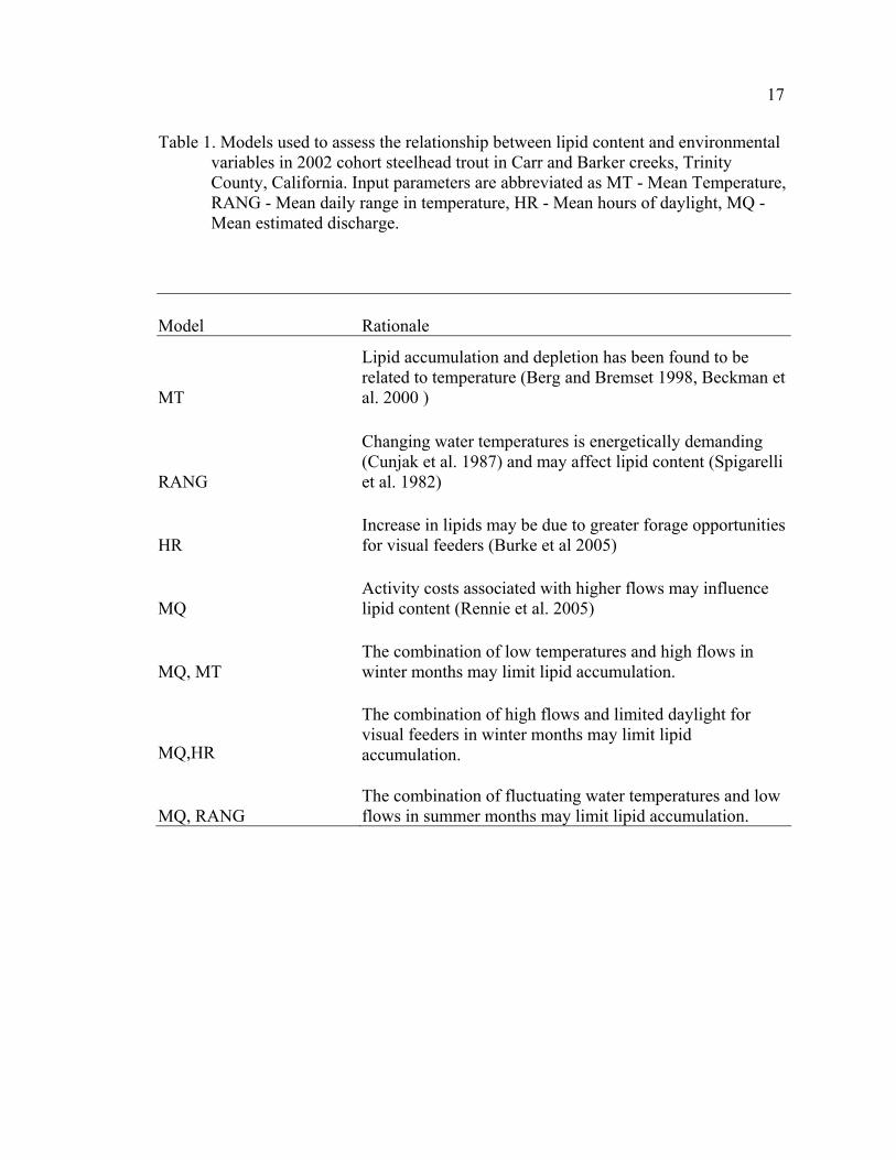
Table 1. Models used to assess the relationship between lipid content and environmental variables in 2002 cohort steelhead trout in Carr and Barker creeks, Trinity County, California. Input parameters are abbreviated as MT - Mean Temperature, RANG - Mean daily range in temperature, HR - Mean hours of daylight, MQ - Mean estimated discharge.

Model Rationale

MT

Lipid accumulation and depletion has been found to be related to temperature (Berg and Bremset 1998, Beckman et al. 2000 )

RANG

Changing water temperatures is energetically demanding (Cunjak et al. 1987) and may affect lipid content (Spigarelli et al. 1982)

HR Increase in lipids may be due to greater forage opportunities for visual feeders (Burke et al 2005)

MQ Activity costs associated with higher flows may influence lipid content (Rennie et al. 2005)

MQ, MT The combination of low temperatures and high flows in winter months may limit lipid accumulation.

MQ,HR

The combination of high flows and limited daylight for visual feeders in winter months may limit lipid accumulation.

MQ, RANG The combination of fluctuating water temperatures and low flows in summer months may limit lipid accumulation.

17

Length-weight relationships of young of the year steelhead trout were investigated

with condition factor, calculated as:

x 105

where a is the condition factor, W is weight, L is length and b is the slope of the fitted

linear regression of loge(W) versus loge(L). To test the isometric growth assumptions in

Fulton’s condition factor, a t-test was used to determine if slopes did not significantly

differ from 3. If slopes did differ from 3.0, comparisons were made to determine if slopes

differed from each other using Analysis of covariance. When a common slope was

achieved, condition factor of 2002 cohort steelhead trout was compared between streams

for each sampling period. An alpha level of 0.05 was used to detect significance in all

statistical analyses. All analyses were conducted using SAS software version 6.12 (SAS

Institute Inc., Cary, North Carolina).

be

e

LWa

)(log)(log

=

18

RESULTS

Habitat

Carr Creek and Barker Creek are both 3rd order streams similar in watershed size,

elevation and slope (Table 2). From habitat measurements taken during the study, Barker

Creek had a greater proportion of riffles (72.3%) and a smaller proportion of runs

(17.4%) and pools (10.3%), than Carr Creek (56.2% riffles, 28.8% runs, and 15.0%

pools). The mean maximum pool depth was similar in Carr Creek and Barker Creek

(0.60 m and 0.66 m respectively).

Environmental Variables

The variation in discharge throughout the study was similar in Carr and Barker

creeks (Figure 4). Five distinct storms occurred during sampling intervals 3, 4 and 5.

The most important difference between sites was in temperature regime (Table 3). The

mean temperatures recorded were warmer in Carr Creek than in Barker Creek during the

summer months (sampling intervals 1 and 6). Temperature varied on a daily basis to a

greater extent in Carr Creek than in Barker throughout the year. Maximum daily

temperature recorded in the early summer (June-August 2003) was on average 5.3

degrees warmer in Carr Creek than in Barker Creek.

19

Table 2. Comparison of Barker Creek and Carr Creek watersheds, Trinity County, California, from topographic maps and summer habitat typing. Watershed metrics provided describe basin conditions above study reaches.

Characteristic Barker Creek Carr Creek

Stream order 3 3

Drainage area (km2) 13.4 16.1

Mean slope in study reach (%) 2 2

Elevation (m) 800 - 920 830 - 940

Mean wetted width (m) 3.7 3.6

Area in pools (%) 10.3 15.0

Mean maximum pool depth (m) 0.66 0.60

Area in riffles (%) 72.3 56.2

Mean riffle depth (m) 0.18 0.15

Area in runs (%) 17.4 28.8

Mean run depth (m) 0.20 0.18

Number of units 60 69

Pool:Riffle Ratio 0.14 0.27

20

4

6

8

10

12

14

16

18

Day

light

(Hrs

)

Figure 4. Mean daily temperature, daily range in temperature, photoperiod, and estimated

mean daily discharge measured in Barker and Carr creeks, Trinity County, California during 2002-2003. Vertical lines indicate sampling periods.

0

2

4

6

8

10

12

14

16

18

20Te

mpe

ratu

reoC

BarkerMean

BarkerRange

CarrMean

CarrRange

0

1

2

3

4

5

6

7

8

7/25/20

02

8/25/20

02

9/25/20

02

10/25/2

002

11/25/2

002

12/25/2

002

1/25/20

03

2/25/20

03

3/25/20

03

4/25/20

03

5/25/20

03

6/25/20

03

7/25/20

03

Date

Dis

char

gem

3s-

1

Barker

Carr

Sampling Period

1 2 4 5 6 3

21

Table 3. Summary statistics of environmental variables included in models of Barker and Carr creeks, Trinity County, California. Interval periods are: 1 = July – September 2002, 2 = September – November 2002, 3 = November 2002 – January 2003, 4 = January – April 2003, 5 = April – June 2003 and 6 = June – August 2003.

Barker Creek

Interval 1 2 3 4 5 6

Days/ interval 51 55 64 83 54 65

Mean temperature oC 12.3 8.4 6.6 6.7 7.9 12

Degree days 627 1088 1512 2179 2599 3379 Mean daily range in temperature oC 2.2 1.7 0.4 1.2 2 2.2 Mean daily maximum temperature oC 13.4 8.9 6.7 7.3 9.2 13.2

Mean hours daylight 13.2 10.9 9.3 10.8 14 14.6

Mean discharge (m3/s) 0.01 0.02 0.63 0.4 0.68 0.07 Standard deviation discharge (m3/s) 0.00 0.02 1.12 0.39 0.71 0.04

Carr Creek

Interval 1 2 3 4 5 6

Days/ interval 59 49 63 84 51 66

Mean temperature oC 14.7 7.9 6 7.8 9.2 15.7

Degree days 868 1264 1638 2294 2752 3802 Mean daily range in temperature oC 4.3 3.8 1.3 2.3 3.5 5.4 Mean daily maximum temperature oC 16.8 9.9 4.9 7.6 11.3 18.5

Mean hours daylight 13.1 10.7 9.3 11.2 14 14.6

Mean discharge (m3/s) 0.01 0.014 0.54 0.23 0.58 0.06 Standard deviation discharge (m3/s) 0.00 0.01 0.98 0.16 0.62 0.03

22

Steelhead Abundance

Density of juvenile steelhead trout varied among habitat types in both Barker and

Carr creeks (Table 4). In Barker Creek, the highest density observed throughout the study in

run habitats (0.75 fish/m2) was recorded in July 2002. Steelhead were generally observed at

higher densities in run habitats than in pools or riffles in Barker Creek. However during the

November sampling period, pools had a higher density of steelhead (0.49 fish/m2) than runs

(0.27 fish/m2) or riffles (0.21 fish/m2). In Carr Creek, the highest density of juvenile

steelhead in was recorded in pool habitats (1.12fish/m2) in August 2003. There was no clear

pattern in steelhead density among the habitat units throughout the study in Carr Creek.

In Barker Creek, one sampling unit 4 feet long was considered complex and excluded

from the population estimate during each sampling period. At the beginning of the study, the

estimated total number of juvenile steelhead in sampled study reaches was higher in Barker

Creek (962) than in Carr Creek (840). In 2002, however, cohort populations were similar in

the two streams (730 and 767, respectively). Abundance in Barker Creek was similar at the

next sampling event in September, but declined in Carr Creek (Figure 5). At the end of the

study, the estimated population of the 2002 cohort was 105 in Carr Creek and 128 in Barker

Creek.

Patterns of Growth

Mean length of 2002 cohort steelhead increased throughout the study period in both

Carr and Barker creeks (Table 5). In Barker Creek, steelhead increased in fork length from

51.8 to 106.0 mm during the study. Absolute growth in Barker Creek was least (9.3 mm)

between the July and September 2002 and greatest (24.1 mm) between April and June 2003.

23

Table 4. Density (number/m2) of steelhead trout (all ages) in runs, pools and riffles in Barker and Carr creeks, Trinity County, California during 2002 and 2003.

Barker Creek

Sampling Period Runs Pools Riffles

Jul-02 0.75 0.56 0.48

Sep-02 0.75 0.61 0.27

Nov-02 0.27 0.48 0.21

Apr-03 0.09 0.06 0.04

Jun-03 0.12 0.11 0.12

Aug-03 0.35 0.31 0.17

Carr Creek

Sampling Period Runs Pools Riffles

Jul-02 0.50 0.52 0.36

Sep-02 0.22 0.39 0.16

Nov-02 0.16 0.14 0.13

Apr-03 0.04 0.03 0.05

Jun-03 0.09 0.07 0.11

Aug-03 0.55 1.12 0.39

24

0

200

400

600

800

1000

1200

1400

July Sept Nov April June Aug

Month

Num

ber o

f Ste

elhe

adBarker Creek total PEAge 0+ Cohort

0

200

400

600

800

1000

1200

1400

July Sept Nov April June Aug

Month

Num

ber o

f Ste

elhe

ad

Carr Creek total PEAge 0+ Cohort

Figure 5. Population estimates for the 2002 cohort and all other age classes of steelhead trout population estimates in Barker and Carr creeks, Trinity County, California 2002-2003.

25

Table 5. Mean length (mm) of 2002 cohort steelhead selected for lipid analysis and all other 2002 cohort steelhead measured in Barker and Carr creeks, Trinity County, California, during 2002-2003. P-values are results of a T-test to compare steelhead size in the two categories.

Lipid samples All remaining steelhead

Date n Mean (mm) σ2 n

Mean (mm) σ2 P-value

Barker Creek

Aug 1, 2002 12 50.4 61.2 109 51.8 59.7 0.553

Sept 21, 2002 13 58.8 29.6 155 61.1 38.5 0.212

Nov 15, 2002 10 62.8 73.7 103 62.1 55.2 0.776

Jan 17, 2003a 5 63.7 9.4

Apr 11, 2003 8 73.1 156.1 46 70.8 94.1 0.490

Jun 3, 2003 8 104.4 545.4 31 94.9 303.7 0.211

Aug 6, 2003 6 106.8 147.4 24 106.0 214.7 0.904

Carr Creek

Jul 30, 2002 13 60.8 56.6 149 64.4 72.6 0.148

Sept 27, 2002 12 66.8 36.8 69 66.4 47.4 0.871

Nov 16, 2002 11 72.5 54.3 49 72.2 98.5 0.915

Jan 17, 2003a 7 63.6 5.9

Apr 12, 2003 14 83.8 165.1 42 84.8 241.1 0.821

Jun 1, 2003 6 101.7 151.5 20 105.1 299.6 0.600

Aug 7, 2003 6 101.7 27.5 19 120.1 299.0 < 0.001* a All steelhead collected during the January sampling period were used for lipid analysis.

26

Post comparison of means in Barker Creek revealed no significant increase in length between

the September and November sampling periods, but increases were significant between all

other sampling periods (Table 6). Year 2002 cohort steelhead were consistently longer in

Carr Creek than in Barker Creek, but not significantly so (ANOVA df = 11, p-value = 0.52).

In Carr Creek, steelhead increased in fork length from 64.4 mm in July 2002 to 120.1 mm in

August 2003. Absolute growth in Carr Creek was least (2.0 mm) between the July and

September 2002 and greatest (20.3 mm) between April and June 2003. Post comparison of

means in Carr Creek revealed that there was no significant increase in length between July

2002 and September 2002 or between June 2003 and August 2003 (Table 6).

Mean weight of 2002 cohort steelhead increased throughout the study period in both

Carr and Barker creeks (Table 7). In Barker Creek, steelhead increased in weight from 1.70

to 15.50 g during the study. Absolute growth in weight in Barker Creek was also least (0.20

g) between September and November 2002 and greatest (6.76 g) between April and June

2003. The weight of 2002 cohort steelhead differed among sampling periods in Barker

Creek (df = 5, p=0.001) and post comparison of means revealed that there was no significant

increase in weight between the September 2002 to November 2002 sampling interval (Table

6). Mean weight of year 2002 cohort steelhead was consistently greater in Carr Creek than in

Barker Creek, but not significantly so (ANOVA df = 11, p = 0.54). In Carr Creek, steelhead

increased in weight from 3.29 g in July 2002 to 20.80 g in August 2003. Absolute growth in

Carr Creek was least (0.08 g) between the July and September 2002 and greatest (6.65 g)

between April and June 2003. The weight of 2002 cohort 0+ steelhead differed among

sampling periods in Carr Creek (df=5, p=0.001) and post comparison of means revealed

27

Table 6. Results of Student Newman-Keuls multiple comparison test performed on log transformed fork length (FL) and weight (WT) for 2002 cohort steelhead in Barker and Carr creeks, Trinity County, California during 2002-2003. Horizontal bars indicate groups with no significant difference.

Barker Creek July Sept Nov Apr June Aug FL (mm) P < 0.01

WT (g) P < 0.01

Carr Creek FL (mm) P < 0.01

WT (g) P < 0.01

28

Table 7. Mean wet weight (g) of 2002 cohort steelhead selected for lipid analysis and all other 2002 cohort steelhead measured in Barker and Carr creeks, Trinity County, California during 2002-2003. P-values are results of t-test to compare steelhead size in the two categories.

Lipid samples All remaining fish measured

Date N Mean Wt (g) σ2 n

Mean Wt (g) σ2 P-value

Barker Creek

Aug 1, 2002 12 1.52 0.44 109 1.70 0.57 0.436

Sept 21, 2002 13 2.13 0.34 155 2.50 0.56 0.083

Nov 15, 2002 10 2.74 1.12 103 2.70 0.89 0.907

Jan 17, 20031 7 3.22 1.21

Apr 11, 2003 8 5.28 7.76 46 4.96 4.83 0.337

Jun 3, 2003 8 15.84 100.91 31 11.72 48.51 0.182

Aug 6, 2003 6 15.50 31.24 24 15.35 50.19 0.963

Carr Creek

Jul 30, 2002 13 2.66 0.96 149 3.29 1.52 0.074

Sept 27, 2002 12 3.26 0.85 69 3.37 1.20 0.739

Nov 16, 2002 11 4.07 1.80 49 4.38 3.25 0.598

Jan 17, 20031 7 3.10 0.99

Apr 12, 2003 14 7.69 9.12 42 8.96 27.85 0.274

Jun 1, 2003 6 12.55 19.23 20 15.61 86.16 0.340

Aug 7, 2003 6 12.19 3.68 19 20.80 74.22 0.001*

1 All steelhead collected during the January sampling period were used for lipid analysis.

29

that there was no significant increase in weight between the July 2002 to September 2002

sampling interval (Table 6).

Following an F-test for equality of sample variances, the appropriate t-test (assuming

equal variance or assuming unequal variance) was used to compare the length (Table 5) and

weight (Table 7) of 2002 cohort lipid steelhead to the rest of 2002 cohort measured steelhead

for each sampling period in each stream. Length and weight measurements of steelhead

collected for lipid analysis were significantly different from the measured steelhead in Carr

Creek during August 2003. No significant differences occurred during the remaining

sampling periods in Carr Creek. In Barker Creek, length and weight of steelhead collected

for lipid analysis were not significantly different than the measured steelhead during any of

the sampling periods.

Whole body lipid content of 2002 cohort steelhead increased throughout the study in

both creeks (Figure 6). In Barker Creek, lipid content increased from a mean of 28 mg/fish

in July 2002 to 751 mg/fish in August 2003. In Carr Creek, lipid content increased from a

mean of 132 mg/fish in July 2002 to 852 mg/fish in August 2003. The lipid content of 2002

cohort steelhead in Barker Creek increased during the first sampling interval from 28 mg/fish

in July 2002 to 47 mg/fish in September 2002. In contrast, lipid content in Carr Creek

remained relatively steady during the first sampling interval. Mean lipid content remained

steady from September 2002 to January 2003 in both creeks, and then increased through the

rest of the study. The period of greatest increase in whole body lipid content occurred during

the April 2003 to June 2003 for both Barker Creek (632 mg/fish increase) and Carr Creek

(432 mg/fish increase).

30

Figure 6. Whole body lipid content (mg/fish) and percentage lipids for 2002 cohort steelhead

in Barker and Carr creeks, Trinity County, California during 2002-2003. Error bars depict the 95 percent confidence intervals on estimated means.

0

2

4

6

8

10

July Sept Nov Jan April June AugMonth

Perc

ent L

ipid

Barker Creek % lipid

Carr Creek % lipid

0

200

400

600

800

1000

1200

July Sept Nov Jan April June Aug

Month

Tota

l Lip

id C

onte

nt (m

g/fis

h)

Barker Creek lipid weight

Carr Creek lipid weight

31

Percentage lipid increased overall throughout the study in both creeks (Figure 6). In

Barker Creek, percentage lipid increased from 1.84% in July 2002 to 4.63% in August 2003.

In Carr Creek, percentage lipid increased from 4.87% in July 2002 to 6.98% in August 2003.

During the first sampling period, mean percentage lipids increased from 1.84% to 2.17% in

Barker Creek, while mean percentage lipids decreased from 4.87% to 2.82% in Carr Creek.

In Barker Creek, lipids increased from September 2002 to November 2002, and then

decreased from November 2002 to January 2003. In Carr Creek, lipids remained steady from

September 2002 to January 2003. From April 2003 to August 2003, percentage lipids

increased in both streams. Percentage lipid was higher in Carr Creek than in Barker Creek

during most sampling periods.

Relative Growth Rates

The general pattern of relative growth rates for 2002 cohort steelhead was similar in

the two streams throughout the study, but differences did occur (Figure 7). During the July

to September sampling interval in Barker Creek, relative growth in weight and lipids

increased at the second highest rates observed during the study. Lipid weight decreased in

Carr Creek during the July to September interval without relative growth in length or weight.

Lipids increased during the next sampling interval in both streams. An early winter decline

in lipids was observed during the November to January interval in both Barker and Carr

creeks. April through June was a period of high relative growth in length, weight and lipid in

both streams. During the April 2003 to June 2003 sampling interval, the lipid relative growth

rate for Barker Creek (6.7%/day) was over twice that of Carr Creek (3.0%/day).

32

-1

0

1

2

3

4

5

6

7

8

Jul - Sept Sept - Nov Nov - Jan Jan - Apr Apr - Jun Jun - Aug

Barker relative growth length

Barker relative growth weight

Barker relative growth lipid

-3

-2

-1

0

1

2

3

4

5

6

7

8

Jul - Sept Sept - Nov Nov - Jan Nov/Jan - Apr Apr - Jun Jun - Aug

Carr relative growth length

Carr relative growth weight

Carr relative growth lipid

Figure 7. Relative growth calculations for length, weight and lipid content in 2002 cohort steelhead in Barker and Carr creeks, Trinity County, California during 2002-2003.

33

Production

Total production during the study was higher in Carr Creek (63.2 kg/ha) than in

Barker Creek (55.0 kg/ha) (Table 8). During the July to September interval, production in

Barker Creek was ten times higher than in Carr Creek. Production was lowest in Barker

Creek during the September to November interval. Production was lowest in Carr Creek

during the July to September interval. The April to June interval was the period of highest

productivity for 2002 cohort steelhead in both streams.

Relations to Environmental Conditions

January sampling data were included in this analysis to examine early winter impacts

on lipid reserves. The five 2002 cohort steelhead collected from Barker Creek in January had

a mean of 2.05 percent lipid (Figure 6). The seven 2002 cohort lipid steelhead collected from

Carr Creek in January had a mean of 2.70 percent lipid. These steelhead were included in

general linear models examining lipid content relations to environmental variables.

As is typical of the Pacific Northwest region, Carr and Barker creeks underwent

significant seasonal changes in flow and temperature. Water temperatures and temperature

variation were highest during summer and lowest during winter. Discharge was highest

during winter with concurrent increases in variability. As a result, predictor variables in

many models were correlated in Barker Creek (Appendix A) and Carr Creek (Appendix B).

Of the models without significant multicollinearity, variation in total lipid content was best

modeled as a positive relationship for both mean discharge and day length in Barker Creek

(R2 = 0.595, Table 9) and as a positive relationship for both mean discharge and range in

daily temperature in Carr Creek (R2 = 0.697).

34

Table 8. Mean biomass per area sampled and production estimates during the study for 2002 cohort of steelhead in Barker and Carr creeks, Trinity County, California, during 2002-2003.

Barker Creek Carr Creek

Sampling Interval

Mean biomass/area

(kg/ha) Production

(kg/ha)

Mean biomass/area

(kg/ha) Production

(kg/ha)

Jul – Sept 6.6 5.3 9.0 0.5

Sept - Nov 7.0 1.4 5.1 5.0

Nov – Apr 3.9 8.9 4.0 17.4

Apr – Jun 2.9 22.4 3.4 24.4

Jun – Aug 5.5 17.0 5.3 16.0

Total Production (kg/ha) 55.0 63.2

35

Table 9. Model results of relationships between lipid weight and environmental variables in Barker and Carr creeks, Trinity County, California during 2002-2003. For selected models, the influence of independent variables on lipid content (+) (-), R-square (R2), AIC, change in AIC (Δi), and relative Akaike weights (wi) are shown.

Stream R2 p-value (Δi) AIC wi

Barker Creek

MQ (+), HR (+) 0.595 0.0001 -28.94 0.9369

MQ (+), RANG (+) 0.551 0.0001 5.40 -23.53 0.0628

MQ (+), MT (+) 0.441 0.0001 11.36 -12.18 0.0002

HR (+) 0.248 0.0002 13.39 1.22 2.83E-07

MQ (+) 0.193 0.0011 3.70 4.91 4.46E-08

RANG (+) 0.054 0.0978 8.26 13.17 7.17E-10

MT (-) 0.001 0.8639 2.85 16.02 1.73E-10

Carr Creek

MQ (+), RANG (+) 0.697 0.0001 -59.00 0.9999

MQ (+), HR (+) 0.579 0.0001 18.33 -40.67 0.0001

MQ (+), MT (+) 0.438 0.0001 16.22 -24.45 3.15E-08

HR (+) 0.254 0.0001 13.83 -10.63 3.14E-11

MQ (+) 0.172 0.0015 5.85 -4.78 1.69E-12

RANG (+) 0.049 0.1000 7.75 2.97 3.5E-14

MT (+) 0.025 0.2460 1.42 4.39 1.72E-14

36

Condition Factor

Condition of steelhead trout varied between streams, but also exhibited a common

seasonal pattern of biological interest. Maximum condition of steelhead was recorded in

both streams in November at the beginning of the winter period. In Barker Creek, condition

increased from summer through fall. After November, it declined through spring and

summer. In Carr Creek, condition recorded in both summer sampling periods was only

slightly less than in November, while being low in spring and fall.

Length and weight relationships of steelhead trout were not isometric (slope = 3) in

the two streams on all sampling dates (Table 10). In Barker Creek, the slope of the length

weight relation differed from 3 during the July and November sampling events. In Carr

Creek, the slope differed from 3 during the July sampling event. ANCOVA analysis did not

provide a common slope for 2002 cohort steelhead between streams during the July sampling

period. And therefore, condition factor was not compared between streams for this time

period.

37

Table 10. Sample size (N), slope, condition factors, and adjusted R2 (Adj. R2) of the fitted linear regression of loge(W) versus loge(L) for 2002 cohort of steelhead in Barker and Carr creeks, Trinity County, California during 2002 and 2003.

Barker Creek Carr Creek

Month N Slope Condition

Factor Adj. R2 N Slope Condition

Factor Adj. R2

July 121 3.10a 0.524 0.98 162 2.831 2.416 0.94

Sept 168 3 1.407 0.92 81 3 0.883 0.96

Nov 112 2.82a 2.262 0.95 60 3 2.965 0.96

Apr 54 3 1.060 0.92 56 3 1.007 0.95

Jun 19 3 1.037 0.95 20 3 1.397 0.96

Aug 30 3 0.570 0.97 30 3 2.167 0.97

a Slopes were significantly different from 3 using a t-test, and no common slope was achieved for the two streams in one season using ANCOVA.

38

DISCUSSION

Patterns of growth in fish are influenced by the interplay of overlapping

environmental conditions, which vary seasonally. The growth strategies employed with

available resources and limitations, in combination with behavioral tactics, have strong

implications for survival. In this study, selection of two watersheds similar in environmental

setting, but with different temperature regimes, allowed for a description of observed growth

strategies in response to different thermal patterns. In addition, changes in photoperiod and

stream flow were investigated to examine which environmental condition influences growth

patterns and, in particular, lipid stores for young of the year steelhead trout throughout the

year. Both similarities and differences in growth patterns and population characteristics were

observed between the two streams.

Water temperature has a great effect on poikilothermic organisms. Higher water

temperatures increase rates of development from egg to fry and elevate metabolic activity,

increasing rates at which consumed food is converted to somatic or energetic growth. When

temperatures are within the range of physiological tolerance and an ample food supply is

available, greater size can be achieved. The 2002 cohort of steelhead in Carr Creek were

longer, heavier and had larger lipid reserves than their Barker Creek counterparts at the start

of the first sampling period. Higher mean temperatures and a greater range in daily

temperature during early development of the Carr Creek 2002 cohort may have resulted in

the greater size and lipid stores by the start of the first summer sampling period.

Throughout their first summer, however, it does appear that environmental conditions

were not favorable for growth for Carr Creek steelhead, as evidenced by the significant use

of lipid reserves and very limited somatic growth during summer months. In addition, the

39

population decline in Carr Creek during summer months, as mortality or emigration, was the

greatest observed throughout the study (Forseth et al. 1999). Production estimates during the

first sampling interval in Carr Creek were the lowest observed throughout the study. These

observations suggest that summertime conditions are taxing for young of the year steelhead.

Biomass during that interval was the highest observed during the study. Zorn and Muhfer

(2007) observed that biomass density of brook and brown trout within a year class to have a

negative “density dependent” effect on growth of those species.

In contrast, Barker Creek steelhead trout exhibited summer growth in length and

weight during their first summer. This somatic growth during the July- August sampling

period occurred at the expense of lipid reserves, consistent with the findings of Post and

Parkinson (2001). Production estimates were ten times higher in Barker Creek than in Carr

Creek during this time period. Barker Creek steelhead started out much smaller and with

lower lipid content than the Carr Creek steelhead, emphasizing the importance of the first

summer growing season in Barker Creek.

Lipid anabolism continued in Carr Creek throughout the fall, while there was a slight

increase in lipid content in Barker Creek steelhead. Acclimatization to declining water

temperatures can be energetically demanding (Cunjak et al. 1987). The rate of water

temperature decline was more substantial in Carr Creek. If food supplies were limited, lipid

reserves may have been utilized to meet the increased energy demand to adjust to declining

water temperatures. yet percent lipid in Carr still remained higher than in Barker Creek

However, ample food supplies may offset increased energy demands to adjust to cooler water

temperatures. Collecting information on food supply was beyond the scope of this study and

so the reason for lipid declines is unknown.

40

Neither population demonstrated the fall period of growth observed by Reeves

(1979). However, Reeves described rain events as the trigger for fall growth, and there were

no significant rain events prior to the November sample period in this study. Steelhead from

both streams entered winter with similar lipid stores.

The factors that limit over winter survival have been studied for a number fish

species. Early winter energy depletions observed by Cunjak et al. (1987) in brook trout

populations were attributed to acclimatization to cooling water temperatures and energy

intake insufficient to meet metabolic activity. This may have been the cause of declines in

lipid reserves for Barker Creek during the early winter period from November to January

In areas with sustained harsh winter conditions, the accumulation of energy stores is

essential to sustain individuals though periods of starvation. Many authors have reported

increased over winter survival with increased fish length (Thompson et al. 1991, Hunt 1969,

Oliver et al. 1979) because the smaller fish use energy reserves at a faster rate than larger fish

(Miranda and Hubbard 1994). Cunjak et al. (1987) suggested that metabolic deficiencies are

a result of an inability to assimilate food rather than prey availability during low water

temperatures. However his studies were conducted in a region with prolonged minimum

winter temperatures of 0.1 to 1.5 oC. In this study, winter water temperatures rarely dipped

below 4 oC, and were usually near 6 oC. Warmer water temperatures increase standard

metabolic rates. Limited food availability during winter combined with increased sustained

metabolic costs at warmer temperatures may present physiological challenges to steelhead

trout, particularly to the larger individuals (Connolly and Peterson 2003).

Beckman et al. (2000) found that average body lipid levels increased in February –

March in Yakima River juvenile Chinook salmon at some sites. An effort was made in my

41

study to sample each creek earlier in the spring, however high flows prevented capturing

enough steelhead trout for an adequate sample. From January to April, lipid content of

steelhead trout in Carr Creek increased by an average of 1 percent, and in Barker Creek lipid

content increased to a lesser extent (0.2 percent). Other researchers have found increased

lipid content during late winter/early spring when temperatures are still low (Cunjak et al.

1987), and have attributed these anabolic processes to changing photoperiod (Beckman et al.

2000). The results from Barker Creek in this study agree with those findings,, the top model

shows a positive relationship between hours of daylight and lipid content.

This study identified early spring as a period of rapid anabolism as reflected in all

types of growth, with preference to somatic growth. This is similar to the research of Berg

and Bremset (1998), who found increases in percentage body lipid from April to June in

populations of Atlantic salmon and brown trout. Throughout the study, the 2002 cohort in

Carr Creek had generally faster growth rates than Barker Creek, and lipid content in Carr

Creek steelhead trout was overall higher than that of Barker Creek. This is consistent with

the work of Post and Parkinson (2001) who proposed that rainbow trout of the same size tend

to have higher lipid content in aquatic systems that support faster growth rates.

Model results for both Carr and Barker creeks in this study show a positive

relationship between mean discharge and lipid content in both streams in top models. This

was not what I expected. I thought that greater discharge in winter months would tax young

steelhead because of the energy expended to maintain their position and feed at high water

levels. These model results appear to be a result of the April to June 2003 interval that had

the highest increase in lipid content observed throughout the study and also highest mean

flow. Perhaps high flow and flood events provided a greater food supply for young of the

42

year steelhead by dislodging macroinvertebrates from instream substrate or riparian habitats

(White and Harvey 2007).

Condition factor indices have been widely used as an index of the health and

robustness of fish with the assumption that increases in weight are reflective of increases in

fat tissue. Some researchers have found relatively high correlations between condition factor

and percent fat (Herbinger and Friars 1991). This would support the steady increases in both

Fulton’s condition factor and percentage lipid that was observed in Carr Creek. However,

other researchers have found low correlations between Fulton’s condition factor and

percentage fat (Simpson et al. 1992). In Barker Creek, increases were not consistent between

percentage lipid and condition factor. The reason for this is unknown,, however, the weak

correlation of water weight of fish to fat weight (Sutton et al. 2000) could contribute to these

findings.

Some researchers consider production rate to be a powerful indicator of a species

ecological success (Le Cren 1969, O’Connor and Power 1976). Production rates are

influenced by water quality of the system, and are the combined result of a population’s

recruitment, growth, total biomass and mortality. Production rates in this study loosely

followed relative growth rates for weight, with population size driving the differences in the

discrete increment summation production calculations. The productive April to June interval

in Barker Creek was influenced largely by growth, while in Carr Creek, high productivity

calculations were influenced by greater biomass due to the larger size of the steelhead.

Carr and Barker creeks produced a similar number of fish at the end of the study.

However, Carr Creek fish were longer, heavier and with greater lipid reserves than their

Barker Creek counterparts, indicating a generally heartier cohort. Condition factor and

43

production metrics support this claim as well. Model results show that diel temperature

fluctuations were positively related to lipid stores, consistent with Spigerelli et al. (1982).

Diel fluctuations were greatest during summer. From field observations, I attribute these

fluctuations in Carr Creek to low flows and limited riparian cover. Although temperature

fluctuations appear to benefit steelhead overall during the study period, there was evidence of

stress during the first summer for young of the year fish. Continued increases in temperature

may have a negative impact on steelhead.

This study provided data that can be useful in understanding survival of steelhead in

the region by identifying periods of anabolism and catabolism in wild populations of juvenile

steelhead over the course of one year. A multi-year project would reveal variability in

physical factors over time and would yield greater insights into growth patterns and their

drivers, as would identification of growth patterns in individual steelhead. Additional studies

that include measurements of available food supply will be able to further narrow the causes

of lipid anabolism and catabolism. Further research should include these elements.

44

LITERATURE CITED

Association of Official Analytical Chemists. 1975. Official methods of analysis. 12th edition. Association of Official Analytical Chemists, Washington DC.

Allen, M. A. 1986. Population dynamics of juvenile steelhead trout in relation to density and

habitat characteristics. Master’s Thesis, Department of Fisheries, Humboldt State University, Arcata California.

Beckman, B. R., D. A. Larsen, C. Sharpe, B. Lee-Pawlak, C. B. Schreck, and W. W.

Dickhoff. 2000. Physiological status of naturally reared juvenile spring Chinook salmon in the Yakima River: Seasonal dynamics and changes associated with smolting. Transactions of the American Fisheries Society 129:727-753.

Berg, O. K., E. Thronaes, and G. Bremset. 2000. Seasonal cycle of body composition and

energy of brown trout (Salmo trutta) in a temperate zone lake. Ecology of Freshwater Fish 9:163-169.

Berg, O. K and G. Bremset. 1998. Seasonal changes in the body composition of young

riverine Atlantic salmon and brown trout. Journal of Fish Biology 52:1272-1288. Bisson, P.A., J.L. Nielsen, R.A. Palmason, and L.E. Grove. 1982. A system of naming

habitat types in small streams, with examples of habitat utilization by salmonids during low streamflow. Pages 62-73 in N.B. Armantrout, editor. Acquisition and utilization of aquatic habitat inventory information. American Fisheries Society, Western Division, Bethesda, Maryland.

Burke, M. G., M. R. Kirk, N. A. MacBeth, D. J. Bevan, and R. D. Moccia. 2005. Influence of

photoperiod and feed delivery on growth and survival of first-feeding Arctic char. North American Journal of Aquaculture 67:344-350.

Burnham, K. P. and D. R. Anderson. 2002. Model selection and multimodel inference: a

practical information–theoretic approach. Second Edition. Springer, New York, New York.

Connolly, P. J., and J. H. Peterson. 2003. Bigger is not always better for overwintering

young-of-the-year steelhead. Transactions of the American Fisheries Society, 132:262-274.

Cunjak, R.A., R.A. Curry, and G. Power. 1987. Seasonal energy budget of brook trout in

streams: Implications of a possible deficit in early winter. Transactions of the American Fisheries Society 116:817-828.

Denton, J. E. and M. K. Yousef. 1976. Body composition and organ weights of rainbow

trout, Salmo gairderi. Journal of Fish Biology 8:489-499.

45

DeVries, D. R. and R. V. Frie. 1996. Determination of age and growth. B. Murphy and D.

Willis, editors. Fisheries techniques. Second Edition. American Fisheries Society, Bethesda, Maryland.

Forseth, T., T.F. Naesje, B. Jonsson and K. Haraker. 1999. Juvenile migration in brown

trout: a consequence of energetic state. Journal of Animal Ecology 68:783-793. Forsman, A. and L.E. Lindell. 1991. Tradeoff between growth and energy storage in male

Vipera berus (L.) under different prey densities. Functional Ecology 5:717-723. Groot, C., L. Margolis, and W.C. Clarke. 1995. Physiological ecology of Pacific salmon.

University of British Columbia Press, Vancouver, British Columbia, Canada. Herbinger, C. M. and G. W. Friars. 1991. Correlation between condition factor and total

lipid content in Atlantic salmon, Salmo salar L parr. Aquaculture and Fisheries Management 22:527-529.

Hirsch, R. M. 1982. A Comparison of four streamflow record extension techniques. Water

Resources Research 18:1081-1088. Hunt, R. L. 1969. Overwinter survival of wild fingerling brook trout in Lawrence Creek,

Wisconsin. Journal of the Fisheries Research Board of Canada 26:1473-1483. Kuehl, R. O. 2000. Design of experiments: statistical principles of research design and

analysis. Second Edition. Duxbury Press, Pacific Grove, California. Larsen, D.A., B. R. Beckman, and W. W. Dickhoff. 2001. The effect of low temperature

and fasting during the winter on growth and smoltification of Coho salmon. North American Journal of Aquaculture 63: 1-10.

Le Cren, E. D. 1969. Estimates of fish populations and production in small streams in

England. Pages 269-280 in T.G. Northcote, editor. Symposium on salmon and trout in streams. H.R. MaxMillan Lectures in Fisheries, University of British Columbia, Vancouver, British Columbia, Canada.

Miranda, L.E. and W. D. Hubbard. 1994. Length dependent winter survival and lipid

composition of Age-0 largemouth bass in Bay Springs Reservoir, Mississippi. Transactions of the American Fisheries Society 123:80-87.

Mohr, M. S. and D. G. Hankin. 2005. Two-phase survey designs for estimation of fish

abundance in small streams. Technical Memorandum, National Oceanic Atmospheric Administration Fisheries, Southwest Fisheries Science Center, Santa Cruz, California. Unpublished.

46

O’Connor, J. F. and G. Power. 1976. Production by brook trout (Salvelinus fontinalis) in four streams in the Matamek watershed, Quebec. Journal of the Fisheries Research Board of Canada 33:6-18.

Oliver, J. D., G. F. Holeton, and K. E. Chua. 1979. Overwinter mortality of fingerling

smallmouth bass in relation to size, relative energy stores, and environmental temperature. Transactions of the American Fisheries Society 108:130-136.

Post, J. R. and E. A. Parkinson. 2001. Energy allocation strategy in young fish: allometry

and survival. Ecology 82:1040-1051. Rand, P. S., B. F. Lantry, R. O'Gorman, R. W. Owens, and D. J. Stewart. 1994. Energy

density and size of pelagic prey fishes in Lake Ontario, 1978-1990: Implications for salmonine energetics. Transactions of the American Fisheries Society 123:519-534.

Reeves, G. H. 1979. Population dynamics of juvenile steelhead trout in relation to density

and habitat characteristics. Master’s Thesis, Department of Fisheries, Humboldt State University, Arcata California.

Rennie, M. D., N. C. Collins, B. J. Shuter, J. W. Rajotte, and P. Couture. 2005. A

comparison of methods for estimating activity costs of wild fish populations: more active fish observed to grow slower. Canadian Journal of Fisheries and Aquatic Science 62: 767-780.

Rikardsen, A. H. and J. M. Elliott. 2000. Variations in juvenile growth, energy allocation

and life-history strategies of two populations of Arctic charr in north Norway. Journal of Fish Biology 56:328-346.

Simpson, A. L., N. B. Metcalfe, and J. E. Thorpe. 1992. A simple non-destructive

biometric method for estimating fat levels in Atlantic salmon, Salmo salar L. parr. Aquaculture and Fisheries Management 23:23-29.

Spigarelli, S. A., M. M. Thommes, and W. Prepejchal. 1982. Feeding, growth, and fat

deposition by brown trout in constant and fluctuating temperatures. Transactions of the American Fisheries Society 111:199-209.

Sutton, S. G., T. P. Bult, and R. L. Haedrich. 2000. Relationships among fat weight, body

weight, water weight and condition factors in wild Atlantic salmon parr. Transactions of the American Fisheries Society 129:527-538.

Thompson, J. M., E. P. Bergersen, C A Carlson, L.R. Kaeding. 1991. Role of size condition

and lipid content in the overwinter survival of age-0 Colorado squawfish. Transactions of the American Fisheries Society 120:346-353.

47

Warren, C. E. and P. Doudoroff. 1971. Biology and water pollution control. W. B. Saunders Co., Philadelphia, Pennsylvania.

White, J. L. and B. C. Harvey. 2007. Winter feeding success of stream trout under different

streamflow and turbidity conditions. Transactions of the American Fisheries Society 136:1187-1192.

Wootton, R. J. 1984. Introduction: strategies and tactics in fish reproduction. In: G. W. Potts

and R. J. Wootton, editors. Fish reproduction: strategies and tactics. Academic Press, London, United Kingdom.

48

Appendix A. Pearson Correlation Coefficients examining correlation between environmental predictor variables in general linear model analysis in Barker Creek, Trinity County, California 2002-2003. Relationships with a coefficient less than 0.75 (shown in bold) were considered adequately free of multicollinearity to be used in modeling. Parameter abbreviations are listed in Table 1.

Barker Creek

MT RANG HR MQ

MT 1 -0.7114 0.7231 -0.7738

RANG 0.7114 1 0.8391 -0.5806

HR 0.7231 0.8391 1 -0.2599

MQ -0.7738 -0.5806 -0.2599 1

49

Appendix B. Pearson Correlation Coefficients examining correlation between environmental predictor variables in general linear model analysis in Carr Creek, Trinity County, California 2002-2003. Relationships with a coefficient less than 0.75 (shown in bold) were considered adequately free of multicollinearity to be used in modeling. Parameter abbreviations are listed in Table 1.

Carr Creek

MT RANG HR MQ

MT 1 0.8195 0.8625 -0.6073

RANG 0.8195 1 0.8049 -0.7042

HR 0.8625 0.8049 1 -0.2668

MQ -0.6073 -0.7042 -0.2668 1

50