SCHRIFTENREIHE ZUR WASSERWIRTSCHAFT

TECHNISCHE UNIVERSITÄT GRAZ

Joerg Koelbl

Process Benchmarking in Water Supply Sector:Management of Physical Water Losses

56

Herausgeber: Univ.-Prof. DDipl.-Ing. Dr.techn. Dr.h.c. Harald Kainz

Technische Universität Graz, Stremayrgasse 10, A-8010 Graz

Tel. +43(0)316 / 873-8371, Fax +43(0)316 / 873-8376 Email: office@sww.tugraz.at, Internet: www.sww.tugraz.at

Verlag der Technischen Universität Graz www.ub.tugraz.at/Verlag ISBN 978-3-85125-055-8

Bibliografische Information der Deutschen Bibliothek: Die Deutsche Bibliothek verzeichnet diese Publikation in der Deutschen Nationalbibliografie; detaillierte bibliografische Daten sind im Internet über http://dnb.ddb.de abrufbar.

Printed by TU Graz / Büroservice

Vorwort des Herausgebers

Wasserverluste aus Trinkwasserversorgungssystemen stellen weltweit eines der größten Probleme hinsichtlich Versorgungssicherheit, aber auch hinsichtlich der hygienischen Qualität des Trinkwassers dar. Auch für Rohrnetze in gutem Zustand ist das Wissen über die Wasserverluste und das Management von Wasserverlusten essentiell. Neben Schadens-raten liefert die Kenntnis über die Höhe der Wasserverluste eines Ver-sorgungssystems wichtige Informationen für die Instandhaltungsplanung.

Dipl.-Ing. Dr. techn. Joerg Koelbl hat in seiner Dissertation ein Bench-markingsystem für den Prozess des Wasserverlustmanagements in Trinkwassernetzen entwickelt. Dieses System ermöglicht die Analyse der verschiedenen Aufgaben des Wasserverlustmanagements in qualitativer und quantitativer Hinsicht und unterstützt im Erkennen von Stärken und Schwächen und in der Ableitung von Verbesserungsmaßnahmen.

Die Arbeit von Dipl.-Ing. Dr. techn. Joerg Koelbl lieferte auch Beiträge zur ÖVGW Richtlinie W 63 (in Druck), welche parallel zu dieser Disserta-tion überarbeitet wurde. Unter anderem wurde ein neu entwickeltes Klassifikationsschema für Wasserverluste in diese Richtlinie aufgenom-men.

Graz, im Juli 2009

Harald Kainz

3

Acknowledgement This thesis has been developed with the support of several persons to whom I would like to express special thanks. First of all I would like to thank Professor Kainz for giving me the chance to join the University of Technology in 2002. He encouraged me to write this thesis, supervised it and gave helpful input in this work. Special thanks also to Professor Haberl for being the 2nd referee of this thesis and for his comments. Moreover I would like to thank Heimo Theuretzbacher-Fritz for several exciting and informative years of work – especially in the benchmarking projects - and for all his inputs in this thesis. I would like to express thanks to Roland Liemberger for arousing my interest in water loss management and for inspiring me with his stories about water loss management in several parts of the world. Roland has also supported my participation in the IWA Water Loss Task Force (WLTF) as well as the IWA LAMIC Task Force – thereby creating very valuable contacts for this thesis. Beside Roland I also would like to thank Dewi Rogers for the work in the NRW Management Process Mapping Initiative of the WLTF. Some aspects of this initiative have been used in this thesis. I would also like to thank Allan Lambert for numerous emails discussing the challenges in calculating the Infrastructure Leakage Index. Special thanks also to David Main and Peter Stahre for sharing information about benchmarking projects in Canada and in Scandinavia. Thanks are also expressed to Peter Martinek and Dieter Martinek for their support and for sharing information about multi-parameter measurements. Also I would like to express thanks to the Austrian Association for Gas and Water (OVGW) and all participating water utilities for enabling and supporting the Austrian benchmarking projects in the water supply sector. Together with my project colleagues from University of Natural Resources and Applied Life Sciences in Vienna several benchmarking projects have been carried out - fruitful years of work, for which I would like to thank Roman Neunteufel, Ernest Mayr and Reinhard Perfler. Also I would like to thank all members of the working group for the OVGW directive W 63 about water losses for their critical comments and the exciting discussions. Special thanks are expressed to my former employers Christian Kaiser and Thomas Mach who gave me the opportunity to practice planning of water supply and sewerage systems. I would like to thank all members of our Institute for their colleagueship. I will treasure countless discussions with Professor Kauch, Daniela Fuchs-Hanusch, Gerald Gangl and Franz Friedl and others. Special thanks to Gerryshom Munala from Kenya for proof reading this thesis and for sharing information about the challenges in water management in Africa. The person who has been mainly responsible for my way back from the private sector to university in 2002 is my uncle Franz Mascher – I would like to thank him for his support. Last but not least I would like especially thank my parents for their support over all the years.

4

Preface of Author Water losses from drinking water supply systems are one of the greatest problems worldwide not only regarding supply safety (quantity) but also regarding the provision of safe potable drinking water (quality). Many water supply systems are in such a bad condition that only an intermittent supply with water is possible and more than the half of the water is often lost on the way to the customer. Intermittent supply causes an especially high risk of contamination by entering the water distribution system through leaks. Decision makers often tend to try solving the problem by opening up new resources but this is a fight against the symptoms and not against the real causes. Figure 1 humorously aids understanding of the crucial point of the problem. But the knowledge about water losses and the management of water losses is also still very important if the supply network is in good condition. Water losses are the only directly measureable indicator for the condition of a pipe network and are, therefore, an important basis for maintenance and rehabilitation planning. Due to different frame conditions (e.g. the structure of supply network or resources available), but also due to the rapid development of technical equipment for leakage monitoring and leak detection, it is difficult for a single water utility to find the best water loss management strategy and to adopt the own strategy. Therefore, the need for a system that enables a comparison of the process of water loss management regarding effectiveness and efficiency has become apparent. This is one of the motivations for this work, which has the purpose of developing a process benchmarking system for the process of water loss management. This system should support process analyses and the derivation of optimisation measures to achieve best practices in water loss management for individual utilities.

Figure 1: Understanding the problem of leakage (source: Water and Sanitation Program of the World Bank, in LIEMBERGER 2007)

5

Vorwort des Autors Wasserverluste aus Trinkwasserversorgungssystemen stellen weltweit eines der größten Probleme hinsichtlich Versorgungssicherheit (Quantität der Versorgung), aber auch hinsichtlich hygienischer Qualität des Wassers dar. Viele Wasserver-sorgungssysteme sind in einem derart schlechten Zustand, dass keine kontinuierliche Versorgung mit Trinkwasser möglich ist. Häufig geht in solchen Systemen mehr als die Hälfte des Wassers am Weg zum Kunden verloren. Diskontinuierliche Versorgung bringt auch ein enormes hygienisches Risiko mit sich, da über Leckagen Verunreinigungen ins Rohrnetz gelangen können. Entscheidungsträger erkennen das wahre Problem der Wasserverluste häufig nicht und tendieren oft dazu, eher die Symptome als die Ursachen zu bekämpfen. Figure 1 bringt das wahre Problem in einer lustigen Art und Weise auf den Punkt. Aber auch für Rohrnetze in gutem Zustand ist das Wissen über die Wasserverluste und das Management von Wasserverlusten essentiell. Denn Wasserverluste sind der einzig wirklich direkt messbare Indikator für den Zustand der Rohrnetze. Daher stellen Wasserverluste ein wichtiges Entscheidungskriterium für die Instandhaltungs- und Rehabilitationsplanung dar. Aufgrund unterschiedlicher Rahmenbedingungen (z.B. Struktur des Versorgungs-systems oder Verfügbarkeit von Ressourcen) aber auch aufgrund rasant fort-schreitender Entwicklungen neuer Technologien für die Überwachung von Wasser-verlusten und für die Leckortung, ist es für einzelne Wasserversorgungsunternehmen oft schwierig, die individuell optimale Strategie für das Wasserverlustmanagement abzuleiten. Für einen Vergleich des Prozesses des Wasserverlustmanagements hinsichtlich Effektivität und Effizienz fehlen aber bislang geeignete Systeme. Das ist eine der Motivationen für diese Arbeit, die das Ziel hat, ein Prozess-Benchmarking System für den Prozess des Wasserverlustmanagements zu entwickeln. Dieses System soll Prozessanalysen und die Ableitung von Optimierungsmaßnahmen unterstützen, um für Wasserversorgungsunternehmen individuell optimale Strategien für das Wasserverlustmanagement zu erreichen.

6

Abstract In this PhD thesis a benchmarking system for the process of water loss management in drinking water supply systems has been developed. The system is limited to physical (real) water losses. Non-revenue water management is not considered. The process benchmarking system enables analyses of various tasks of water loss management like leakage monitoring, leak detection, analyses and planning as well as infrastructure management and staff qualification. The comparison of water supply utilities allows the identification of strengths and weaknesses of different water loss management strategies and technologies as well as operational approaches. The analyses are based on technical (qualitative) and economical criteria. Exchange of experience between utilities supports the derivation of measures for improvement. Beside some general methodological aspects regarding benchmarking, especially process benchmarking, this PhD thesis provides actual information about water loss management. One aspect is a new classification scheme for water losses which was implemented to the OVGW directive W 63 (in press), which has been revised parallel to this PhD thesis. Kurzfassung In dieser Dissertation wurde ein Benchmarkingsystem für den Prozess des Wasser-verlustmanagements in Trinkwassernetzen entwickelt. Das System beschränkt sich auf die tatsächlichen (realen) Wasserverluste. Das Management der nicht in Rechnung gestellten Wassermengen (engl. non-revenue water) wird nicht berück-sichtigt. Das entwickelte Prozess-Benchmarkingsystem ermöglicht die Analyse der verschiedenen Aufgaben des Wasserverlustmanagements. Dazu gehören die Wasserverlustüberwachung, die Leckortung, Analyse- und Planungsaufgaben sowie das Infrastrukturmanagement und die Mitarbeiterqualifikation. Durch den Vergleich von Wasserversorgungsunternehmen können die Stärken und Schwächen der verschiedenen Strategien im Wasserverlustmanagement, der eingesetzten Technologien und der jeweiligen Arbeitsweisen sowohl in wirtschaftlicher Hinsicht, aber auch hinsichtlich der technischen Qualität untersucht werden. Ein Erfahrungsaustausch zwischen den Unternehmen unterstützt das Ableiten von Verbesserungsmaßnahmen. Neben grundsätzlichen methodischen Aspekten zum Benchmarking, insbesondere dem Prozess-Benchmarking, liefert die gegenständliche Arbeit auch aktuelle Beiträge zum Wasserverlustmanagement. Unter anderem wird ein neu entwickeltes Klassifikationsschema für Wasserverluste auch in die ÖVGW Richtlinie W 63 (in Druck) aufgenommen, welche parallel zu dieser Dissertation überarbeitet wurde.

7

Content 1.  Introduction ...................................................................................................... 14 

1.1.  Challenge .................................................................................................... 14 1.2.  Aim of this thesis ......................................................................................... 16 1.3.  Methodology used ....................................................................................... 17 1.4.  Structure of this thesis ................................................................................. 18 

2.  General framework .......................................................................................... 19 2.1.  EU - Water Framework Directive 2000/60/EC ............................................. 20 2.2.  IWA .............................................................................................................. 23 2.3.  COST Action C18 ........................................................................................ 24 2.4.  ISO TC 224 ................................................................................................. 24 2.5.  Global water loss situation ........................................................................... 25 2.6.  Instruments for performance assurance ...................................................... 26 

2.6.1.  Training programmes .......................................................................... 26 2.6.2.  Laws, standards, directives and guidelines ......................................... 26 2.6.3.  Regulation ........................................................................................... 27 2.6.4.  Performance comparisons and benchmarking .................................... 27 

3.  Performance assessment in water supply sector ......................................... 28 3.1.  IWA Performance Indicator System ............................................................. 28 

3.1.1.  Elements of the PI system ................................................................... 28 3.1.1.1.  Variables ...................................................................................... 28 3.1.1.2.  Performance indicators ................................................................ 29 3.1.1.3.  Context information ...................................................................... 30 3.1.1.4.  Explanatory factors ...................................................................... 30 3.1.1.5.  Data reliability and accuracy ........................................................ 30 

3.1.2.  Structure of the PI system ................................................................... 31 3.1.3.  Relevance for process benchmarking of water loss management ...... 33 

3.2.  Benchmarking in the water supply sector .................................................... 33 3.2.1.  Corporate benchmarking ..................................................................... 34 

3.2.1.1.  Objectives of corporate benchmarking ......................................... 34 3.2.1.2.  Methodology in corporate benchmarking ..................................... 34 

3.2.2.  Process benchmarking ........................................................................ 35 3.2.2.1.  What is process benchmarking? .................................................. 36 3.2.2.2.  Objectives of process benchmarking ........................................... 37 

8

3.2.2.3.  Methodologies in process benchmarking ..................................... 37 3.2.2.4.  Different process benchmarking concepts ................................... 38 

3.2.3.  International experiences in benchmarking ......................................... 39 3.2.3.1.  Australia (IWA/WSAA) ................................................................. 39 3.2.3.2.  Canada ........................................................................................ 40 

3.2.3.2.1.  Canadian process benchmarking on Water Loss Management 41 3.2.3.3.  Germany ...................................................................................... 43 

3.2.3.3.1.  Bavarian benchmarking project EffWB ...................................... 47 3.2.3.4.  The Six-Cities Group Benchmarking (Scandinavia) ..................... 48 

3.2.3.4.1.  The Six-Cities Group process benchmarking on water losses .. 50 3.2.3.5.  Netherlands .................................................................................. 52 3.2.3.6.  North European Benchmarking Co-Operation (NEBC) ................ 53 

3.2.4.  The Austrian OVGW benchmarking initiative ...................................... 55 3.2.4.1.  OVGW Corporate Benchmarking ................................................. 56 

3.2.4.1.1.  Stage A (pilot project) ................................................................ 56 3.2.4.1.2.  Stage B (2004 project) .............................................................. 57 

3.2.4.2.  OVGW Process Benchmarking 2007 ........................................... 58 3.2.4.2.1.  Process 1: Customer meter reading .......................................... 59 3.2.4.2.2.  Process 2: Customer meter replacement .................................. 60 3.2.4.2.3.  Process 3: Construction of new mains ...................................... 60 3.2.4.2.4.  Process 4: Construction of new service connections ................ 60 3.2.4.2.5.  Process 5: Rehabilitation of mains ............................................ 60 3.2.4.2.6.  Process 6: Rehabilitation of service connections ...................... 61 3.2.4.2.7.  Process 7: Water loss management .......................................... 61 3.2.4.2.8.  Process 8: Network inspection .................................................. 61 

4.  Basics of Water Loss Management ................................................................ 62 4.1.  Why Water Loss Management? .................................................................. 62 4.2.  IWA Blue Pages – definitions and standardised water balance ................... 63 4.3.  Four basic methods for managing physical water losses ............................ 68 4.4.  Quantification of Water Losses with Performance Indicators ...................... 70 

4.4.1.  Water Loss Ratio (%) .......................................................................... 70 4.4.2.  Real Losses per Mains Length (m³/km·h) ............................................ 71 4.4.3.  Real Losses per Connection per Day (l/conn·d) .................................. 72 4.4.4.  Real Losses per Connection per Day per Metre Service Pressure

Head (l/conn·d·m) ................................................................................ 72 

9

4.4.5.  Infrastructure Leakage Index (ILI) ........................................................ 72 4.4.6.  Non-Revenue-Water (NRW, %, m³/km·d, l/conn·d) ............................. 77 4.4.7.  Recommended classification schemes ................................................ 78 

4.4.7.1.  ILI (Infrastructure Leakage Index) classification ........................... 78 4.4.7.2.  Classification for real losses per connection per day ................... 79 

4.5.  Active Leakage Control ............................................................................... 82 4.5.1.  Management of District Metered Areas (DMAs) .................................. 82 4.5.2.  Leakage Monitoring without DMAs ...................................................... 84 

4.5.2.1.  Principles of multiparameter measurements ................................ 84 4.5.2.1.1.  Flow and noise measurements.................................................. 85 4.5.2.1.2.  Positioning of multiparameter measurements ........................... 86 4.5.2.1.3.  Interpretation of multiparameter measurements ........................ 86 

4.5.3.  Leak detection ..................................................................................... 87 4.5.3.1.  Leak localising ............................................................................. 89 4.5.3.2.  Leak location (pinpointing) ........................................................... 89 

4.5.3.2.1.  Acoustic techniques .................................................................. 89 4.5.3.2.2.  Non-acoustic techniques ........................................................... 90 

4.6.  Pressure Management ................................................................................ 91 4.7.  Infrastructure Management ......................................................................... 93 

5.  The process benchmarking system for managing physical water losses .. 95 5.1.  General remarks .......................................................................................... 95 5.2.  Process mapping of physical water loss management ................................ 96 

5.2.1.  Sub processes of physical water loss management .......................... 100 5.2.1.1.  Leakage Monitoring ................................................................... 100 5.2.1.2.  Leak detection ............................................................................ 101 5.2.1.3.  Analyses & Planning .................................................................. 102 

5.2.2.  Supporting Processes ....................................................................... 103 5.2.2.1.  Infrastructure Management (Physical Asset Management) ........ 103 

5.2.2.1.1.  Leak Repair ............................................................................. 103 5.2.2.2.  Qualification of staff (Intangible Asset Management) ................. 104 

5.3.  Data collection system ............................................................................... 104 5.3.1.  Data accuracy.................................................................................... 105 5.3.2.  Contact details ................................................................................... 105 5.3.3.  Basis data .......................................................................................... 105 5.3.4.  Water supply system data ................................................................. 106 

10

5.3.5.  Water balance data ........................................................................... 106 5.3.6.  Process specific data ......................................................................... 106 

5.3.6.1.  Data of sub process leakage monitoring .................................... 108 5.3.6.2.  Data of sub process leak detection ............................................ 108 5.3.6.3.  Data of sub process analyses and planning ............................... 108 5.3.6.4.  Data of supporting process infrastructure management ............ 108 

5.3.6.4.1.  Data of supporting process leak repair .................................... 109 5.3.6.5.  Data of supporting process qualification of staff ......................... 109 

5.4.  Process performance indicators ................................................................ 109 5.4.1.  Water loss PIs ................................................................................... 111 5.4.2.  Main process PIs ............................................................................... 111 5.4.3.  PIs of leakage monitoring sub process .............................................. 113 5.4.4.  PIs of leak detection sub process ...................................................... 113 5.4.5.  PIs of analyses & planning sub process ............................................ 115 5.4.6.  Sub-PIs of leak repair supporting process ......................................... 116 5.4.7.  Quality indices ................................................................................... 116 

5.4.7.1.  QI of leakage monitoring sub process ........................................ 116 5.4.7.2.  QI of leak detection sub process ................................................ 118 5.4.7.3.  QI of analyses & planning sub process ...................................... 118 5.4.7.4.  QI of infrastructure management supporting process ................ 119 5.4.7.5.  QI of leak repair supporting process .......................................... 120 5.4.7.6.  QI of staff qualification supporting process ................................ 121 5.4.7.7.  QI of the main process ............................................................... 122 

5.5.  The Process Quality Matrix ....................................................................... 124 5.6.  Verbal descriptions .................................................................................... 135 5.7.  Exchange of experiences and derivation of measures for improvement ... 135 

6.  Field test - the 2007 OVGW process benchmarking ................................... 136 6.1.  Frame conditions ....................................................................................... 136 6.2.  Summary of results .................................................................................... 137 

6.2.1.  Water Loss PIs .................................................................................. 137 6.2.2.  Main process results .......................................................................... 142 6.2.3.  Leakage monitoring sub process results ........................................... 145 6.2.4.  Leak detection sub process results ................................................... 147 6.2.5.  Analyses & planning sub process results .......................................... 150 6.2.6.  Leak repair supporting process results .............................................. 151 

11

6.2.7.  Quality indices results ........................................................................ 153 6.2.8.  Best-practices workshop ................................................................... 156 

6.3.  Methodical experiences of the field test ..................................................... 158 7.  Summary and conclusions ........................................................................... 160 8.  Outlook on future research ........................................................................... 163 References ............................................................................................................ 164 Appendix ............................................................................................................... 171 A1.  Data collection system ............................................................................... 172 

A1.1.  Contact details ...................................................................................... 172 A1.2.  Basis data ............................................................................................. 173 A1.3.  Water supply system data .................................................................... 174 A1.4.  Water balance data ............................................................................... 175 A1.5.  Process specific data ............................................................................ 181 

A1.5.1.  Data of leakage monitoring sub process ........................................... 182 A1.5.2.  Data of sub process leak detection .................................................... 184 A1.5.3.  Data for analyses and planning sub process ..................................... 188 A1.5.4.  Data for infrastructure management supporting process ................... 191 

A1.5.4.1.1.  Data for leak repair supporting process ................................ 192 A1.5.5.  Data for qualification of staff supporting process ............................... 196 

12

Abbreviations ATT Association of Drinking Water from Reservoirs AWWA American Water Works Association BDEW German Association of Energy and Water Industries BGBl. Federal Law Gazette (Bundesgesetzblatt) BMLFUW Austrian Ministry of Agriculture, Forestry, Environment and Water Management CARL Current Annual Real Losses CI Cast Iron (pipe material) CIS Commonwealth of Independent States (former USSR) COST European Cooperation in the field of Scientific and Technical Research DBVW German Alliance of Water Management Associations DMA District Metered Area DVGW German Technical and Scientific Association for Gas and Water DWA German Association for Water, Wastewater and Waste EC European Commission EffWB Investigation of efficiency and quality of communal water supply services in Bavaria (Bavarian benchmarking project in water supply sector) EU European Union Eurostat Statistical Office of the European Communities GIS Geographic Information System GRP Glass-fibre Reinforced Plastic (pipe material) idgF in its current version (used for laws) ILI Infrastructure Leakage Index (water loss performance indicator) ISO International Organisation for Standardisation IWA International Water Association LMSVG Austrian Law on Food Security and Protection of Consumers NEBC North European Benchmarking Co-Operation NRW Non-Revenue Water (water loss performance indicator) OECD Organisation for Economic Co-operation and Development OFWAT Office of Water Services (Regulatory Body in England and Wales) OVGW Austrian Association for Gas and Water PCS Process Control System PE Polyethylene (pipe material)

13

PI Performance Indicator PTKA-WTE Project Management Agency Forschungszentrum Karlsruhe Water Technology and Waste Management Division PVC Polyvinyl Chloride (pipe material) SCADA Supervisory Control and Data Acquisition SGI Services of General Interest TC Technical Committee TWV Austrian Drinking Water Ordinance (Trinkwasserverordnung) UARL Unavoidable Annual Real Losses ÜBV Interplant performance comparison of metropolitan utilities VBGW DVGW regional group “Bavaria” VEWIN Association of Dutch Water Companies VKU Association of Local Utilities WLTF Water Loss Task Force WRG Austrian Water Law (Wasserrechtsgesetz) WSAA Water Services Association of Australia

14

1. Introduction

1.1. Challenge As explained in the preface, water losses represent one of the greatest challenges for water utilities worldwide. A possibility to assess water loss management strategies of water utilities and implemented technologies is the methodology of benchmarking, especially of process benchmarking. In the European Union and worldwide, performance assessment has become one of the most important topics in water supply sector in the past decade. Driven by various frame conditions at a national or international level, e.g. the EU water framework directive 2000/60/EC (EUROPEAN PARLIAMENT 2000), the need for more transparency and modernisation strategies in the monopolistic sector of water supply has become increasingly evident. To enable performance assessments on a standardised frameset of performance indicators, the International Water Association (IWA) published a performance indicator (PI) system (ALEGRE et al. 2000 and 2006), which is the basis for many performance comparisons and benchmarking projects all over the world. Many of the existing benchmarking projects use benchmarking systems on utility level, which analyse the entire performance of a water supply company (note: instead of the term “metric benchmarking” the term “corporate benchmarking” should be used for benchmarking systems on utility level). International experiences have shown that corporate benchmarking is a good detection instrument for hidden optimisation potentials. But it is often difficult to derive measures for improvement on the basis of these data. Therefore it may be necessary to make detailed analyses of various processes. Thus, process benchmarking should display how potentials for improvement can be tapped. Because many of the first approaches of process benchmarking in European countries have been based on global economic considerations but lack a demonstrative analysis of technical aspects, there is a need to develop process performance indicators for the technical tasks of the water supply sector (e.g. OVERATH & MERKEL 2004). One process which so far has not been sufficiently considered in process benchmarking projects is the process of “water loss management”. In fact, water losses are an important indicator for the condition of a pipe network, and water loss management is an important process not only for water utilities with high water losses but also for water utilities with small leakage rates as we often find in Austria or other Central European countries. The IWA “Efficient Operation and Management” Specialists Group is very active in performance assessment and benchmarking but a lot of research in the field of managing water losses has also been done in the past few decades with its Water Loss Task Force (WLTF). Beside providing definitions of a standardised water balance and different water loss performance indicators within the IWA Blue Pages (LAMBERT & HIRNER 2000), many publications describe modern methods of leakage monitoring and leak detection techniques like active leakage control, pressure management, asset management

15

and many other topics (e.g. LAMBERT 2002, BROTHERS 2002, FARLEY & TROW 2003, PILCHER et al. 2007 or MORRISON et al. 2007). It is important for water companies to find the right strategy in water loss management. The costs as well as the benefits for each activity and methodology have to be known to enable the right decisions to be made. Therefore each sub process and each single activity in the field of water loss management has to be analysed in detail. Clearly defined sub processes and activities with a measurable input (e.g. costs for personnel and instruments) and a measurable output (e.g. reduction of losses or detection of water losses) are needed. It is necessary to find indicators – technical and economical - for measuring the input and the output of each process. While water companies have to be effective (this means doing the right things), they also have to be efficient (this means doing the things in the right way with minimal effort). To reach this aim the instrument of process benchmarking can be very helpful. Two existing initiatives on benchmarking the process of water loss management have a strong focus on qualitative comparisons of the process (Canada and the Scandinavian Six-Cities Group project). But, up to now, no systems with systematic quantification of the performance of the process of physical water loss management have been developed. However, such quantification of process performances is absolutely necessary when larger groups of participants are benchmarked. A standardised process performance assessment is also useful for international comparisons. Therefore a challenge that should be solved within this thesis is to work out a system that enables the comparison of the main process as well as of the sub processes of physical water loss management. The quantification of the process performance should take place on the basis of such measurable indicators as those described above. The main parts of this thesis were developed within a process benchmarking project of the Austrian Association for Gas and Water (OVGW). The OVGW started their benchmarking initiative with a pilot project on corporate (metric) benchmarking in 2003/2004. This pilot project was followed by a second project on corporate (metric) benchmarking with 72 water supply utilities representing the half of the water supplied in Austria. In 2007 an initiative on process benchmarking was started, and one of the analysed processes was the management of physical water losses. Beside the OVGW process benchmarking, an initiative of the IWA WLTF deals with mapping the process of non-revenue water (NRW) management. The approach worked out within this initiative is much broader than the OVGW approach, which solely focuses on physical water loss management. The work in the WLTF initiative is still ongoing as this thesis is being written, but has given inspiration for this work, and, further, synergies could be used.

16

1.2. Aim of this thesis The aim of this PhD thesis is to work out a process benchmarking system for the process of water loss management with the focus on the management of physical water losses. The topic of managing non-revenue water (NRW) requires a much broader analyses of many additional activities, but these are not part of this thesis. The process benchmarking system has to be based on recent developments in performance assessment and should cover all aspects of modern water loss management. The process benchmarking system should allow the assessment of the performance of water supply utilities from an economic point of view, as well as from technical quality aspects. It should facilitate finding out whether the strategy used in water loss management is effective or not. If not, the system should give support in finding the right strategy. The system should also show where there is room for improvements within the process operation. This means detecting inefficiencies but also potentials for technical (qualitative) optimisations. Beside this, the process benchmarking system for water loss management has to fulfil the following criteria:

• Clear process structure: The process structure has to be well understandable and all parts of the process (sub processes, supporting processes) have to be well defined.

• Hierarchical process structure: The process structure has to be hierarchical, so that both the overall performance and the performance in single parts of the process can be assessed.

• Practical applicability: The system of process benchmarking has to be in step with actual practices and therefore it has to be developed closely with water supply utility experts.

• For all structures: The system has to be applicable for all structures and all sizes of water supply utilities.

• Simple data gathering: The allocation of costs and other data should be simple. The query of context-information should be accomplished with selective lists to keep the effort as low as possible.

• Transparency: The system has to be a transparent one; “black-box” solutions have to be avoided.

• Data quality: The accuracy and reliability of variables has to be considered.

• Structural parameters: The system should consider different frame conditions of water supply systems to allow a performance comparison in “comparable” groups (clusters).

• Voluntary and anonymous system: The system should be used for voluntary benchmarking and should allow anonymous evaluations.

• Field test: The system has to pass a field test within the Austrian water supply sector. Therefore, a case study with eleven water supply utilities was worked out and the results of this field test are described in this thesis.

17

1.3. Methodology used The first steps within this work were the analyses of common practices in water loss management, which are mainly defined by the IWA Water Loss Task Force, and the analyses of the applicability and benefits of existing (process) benchmarking systems. Two projects which deal with water loss management were analysed in special detail. These are the Canadian benchmarking project and the Scandinavian Six-Cities Group project. The second step was a process mapping to define the process structure of physical water loss management. Next, the process benchmarking system was worked out on basis of the process structure. This includes the definition of variables, context information and performance indicators. Quality indices had to be defined and a quality matrix was created for the evaluation of quality in process operation, which helps to identify performance gaps. Afterwards the process benchmarking system was tested in a field test within the Austrian water supply sector. Eleven utilities participated in the 2007 OVGW process benchmarking. This field test provided useful information about weaknesses within the benchmarking system. Finally, improvements on the basis of the experiences of the field test were implemented into the process benchmarking system (Figure 2).

Figure 2: Course of action

investigation

applicability and benefits of existing 

(process) benchmarking systems

common practices  in water loss management

process mapping

processbenchmarking

system

variables

context information

performance  indicators

quality indices

quality matrix

field test

system improvements

OVGW processbenchmarking 200711 water utilities

definition of processstructure

implementation of experiences of the

field test 

18

1.4. Structure of this thesis The first part of the work (chapter 2) gives a short overview about the general framework in managing water supply utilities in the European Union with reference to the EU water framework directive (Directive 2000/60/EC, EUROPEAN PARLIAMENT 2000) and to the COST C18 Action (note: COST is the acronym for European COoperation in the field of Scientific and Technical Research). Parallel to the COST C18 Action, the ISO (International Organisation for Standardisation) has created an international standardisation for service activities relating to drinking water supply systems and wastewater systems by describing the quality criteria of the service and performance indicators. The second part (chapter 3) focuses on performance assessment in the water supply sector. As well as a short description of the IWA PI-system (ALEGRE et al. 2006) chapter 3 also includes an overview about the basics of benchmarking. The differences between corporate (metric) benchmarking and process benchmarking are explained and existing process benchmarking systems are described. Methodical differences and advantages and disadvantages of various approaches in process benchmarking are worked out (holistic strategy vs. selective strategy). This chapter also includes a description of the Austrian benchmarking activities in the water supply sector. The last theoretical chapter (chapter 4) gives an overview of the state of the art in water loss management. Beside a short description of the IWA Water Loss Task Force standards there are also references to the German standard DVGW W 392 (2003) and to various Austrian standards like OeNorm B 2539 – OVGW W 59 (2005), OVGW W 63 (1993), OVGW W 100 (2007), etc. Chapter 5 is the central part of this thesis, where the developed process benchmarking system for the management of physical water losses is described in detail. The first part of this chapter describes the process structure with definitions of the sub- and supporting-processes. The input- and output-factors and quality criteria of all sub processes are also described. Afterwards, the process benchmarking system with its variables, context information and performance indicators are described in detail (note a detailed description of all variables and context information is shown in the appendix). An essential part of the system is the assessment of the quality of process operation. Therefore all the context information is summarised in a structured quality matrix which allows orientation on where there are potentials for improvement and what measures can be derived. Chapter 6 describes a field test of the new system within the Austrian water supply sector and details the lessons learned in this first project run. Finally, (chapter 7) some conclusions about the new system and the first project run in Austria are made and an outlook (chapter 8) on future research like the extension of this process benchmarking system on the diversified topic of non-revenue water management is given. The appendix includes a detailed description of the data collection system.

19

2. General framework After some decades of building public water supply systems in compliance with high quality standards regarding accessibility, water quality and supply safety, a new aspect has become more important: the performance and the standards of water supply should be attained with less use of resources, which means as efficiently as possible (NEUNTEUFEL et al. 2004). The economic optimisation of the water supply sector under guarantee or optimisation of high quality standards and in compliance with ecological targets can give support in (NEUNTEUFEL et al. 2004):

• easing the burden on public households

• increasing the customer satisfaction regarding water quality, supply safety and customer service.

Therefore increasing pressure from various interest groups in the water supply sector (as a part of services of general interest) was seen during the last decade of the 20th century. The European Commission with its intentions and discussions about liberalisation, modernisation and performance of services of general interests was an especially strong driving force for the development of performance evaluation systems for the water supply sector. The understanding of quality, efficiency, standards and demands for the water supply sector strongly depends on the point of view of different observers. Table 1 gives an example:

Table 1: Standards and demands for water supply utilities (according to GIRSBERGER 2003 in THEURETZBACHER-FRITZ et al. 2006)

who understanding for quality frame of reference

politicians low water price

public interest sustainable use of water effective administration

managing director

satisfied customers and authorities

performance assignment less complaints

good staff enough budget

technical director ensured water quality

efficient and unproblematic operation sufficient pressure and volume of water

no interruptions of supply

quality manager fulfilment of quality standards

all business objectives measures for improvement

chemistry compliance with parameter and indicator parameter values food law

Whereas the European Commission is still thinking about the possibilities for liberalisation, the European Parliament refused the liberalisation of the drinking water supply sector with its decision from December 2003 (EUROPEAN PARLIAMENT 2003, COM(2003) 270 – (2003/2152(INI), A5 0484/2003, Pte. 48-49) to the Green Paper on services of general interests (EUROPEAN COMMISSION 2003). Beside other measures,

20

chiefly performance comparisons, like benchmarking, should be implemented to ensure modernisation and to increase the efficiency of the drinking water supply sector (EUROPEAN PARLIAMENT 2003):

A5 0484/2003: The European Parliament… 48)…considers that liberalisation of water supply (including wastewater disposal) should not be carried out in view of the distinctive regional characteristics of the sector and local responsibility for provision of drinking water as well as various other conditions relating to drinking water; calls, however, without going as far as liberalisation, for water supply to be 'modernised' and for the principle of equal treatment of public and private companies to be enforced by means of a variety of individual measures involving limited market opening and the removal of restrictions on competition. 49)…takes the view that benchmarking, economic-efficiency testing, cooperation and efficiently structured undertakings should also be sought in water management, and that a good many specific measures providing limited openings to the market short of full liberalisation will impact favourably on security of supply, price structures and the protection of ground water and the environment.

It is necessary to implement measuring systems with a feedback function in order to evaluate the fulfilment of various demands on the water supply sector in an understandable way and to enable learning from better performing utilities. Benchmarking is such a measuring system with a feedback function (THEURETZBACHER-FRITZ et al. 2006). Several European countries, e.g. Germany, consider benchmarking to be an efficient instrument for identifying, getting acquainted with, and adopting successful methods and processes from benchmarking partners. Therefore, the benchmarking concept of the German water sector is part of the modernisation strategy for the regulatory framework of the German federal government. In 2005 several German Associations of the water sector signed the extended “Statement of the Associations of the Water Industry on Benchmarking in the Water Sector” and thus defined for themselves the support of benchmarking to be an integral part of their self-administration (PROFILE OF THE GERMAN WATER INDUSTRY 2008). The Austrian water supply utilities and their umbrella organisation OVGW also decided to implement the methodology benchmarking as a suitable instrument for performance evaluation, performance presentation and for improving quality and efficiency.

2.1. EU - Water Framework Directive 2000/60/EC In October 2000 the European Parliament and the Council of the European Union enacted the most important law for the European water sector – directive 2000/60/EC (water framework directive) establishing a framework for Community action in the field of water policy. The purpose of the water framework directive is to establish a framework for the protection of inland surface waters, transitional waters, coastal waters and groundwater which (EUROPEAN PARLIAMENT 2000):

21

(a) prevents further deterioration and protects and enhances the status of aquatic ecosystems and, with regard to their water needs, terrestrial ecosystems and wetlands directly depending on the aquatic ecosystems; (b) promotes sustainable water use based on a long-term protection of available water resources… and thereby contributes to:

• the provision of the sufficient supply of good quality surface water and groundwater as needed for sustainable, balanced and equitable water use,

• a significant reduction in pollution of groundwater… The article 4 of the water framework directive deals with environmental objectives and explains how to handle the river basin management plans. Concerning ground water one of the objectives is:

…member states shall protect, enhance and restore all bodies of groundwater, ensure a balance between abstraction and recharge of groundwater, with the aim of achieving good groundwater status at the latest 15 years after the date of entry into force of this directive…

In article 5 the member states are called on to ensure that for each river basin district within its territory:

• an analysis of its characteristics,

• a review of the impact of human activity on the status of surface waters and on groundwater, and

• an economic analysis of water use is undertaken according to the technical specifications set out in Annexes II and III and that it is completed at the latest four years after the date of entry into force of this directive. Annex III of the water framework directive describes the economic analysis:

The economic analysis shall contain enough information in sufficient detail (taking account of the costs associated with collection of the relevant data) in order to: (a) make the relevant calculations necessary for taking into account under Article 9 the principle of recovery of the costs of water services, taking account of long term forecasts of supply and demand for water in the river basin district and, where necessary:

• estimates of the volume, prices and costs associated with water services, and

• estimates of relevant investment including forecasts of such investments;

(b) make judgements about the most cost-effective combination of measures in respect of water uses to be included in the programme of measures under article 11 based on estimates of the potential costs of such measures.

22

Article 9 of the water framework directive is very important for the water supply sector, as it claims cost recovery for water services:

… member states shall take account of the principle of recovery of the costs of water services, including environmental and resource costs, having regard to the economic analysis conducted according to Annex III, and in accordance in particular with the polluter pays principle. Member states shall ensure by 2010:

• that water-pricing policies provide adequate incentives for users to use water resources efficiently, and thereby contribute to the environmental objectives of this directive,

• an adequate contribution of the different water uses, disaggregated into at least industry, households and agriculture, to the recovery of the costs of water services, based on the economic analysis conducted according to annex III and taking account of the polluter pays principle.

Member states may in so doing have regard to the social, environmental and economic effects of the recovery as well as the geographic and climatic conditions of the region or regions affected…

On the basis of the results of analysis specified in article 5 of the directive, the member states have to ensure the establishment of programmes of measures in order to achieve the objectives established under article 4. According to article 11, each programme of measures shall include the “basic” measures and, where necessary, “supplementary” measures. “Basic measures” are the minimum requirements to be complied with and shall consist of:

(a) those measures required to implement Community legislation for the protection of water, including measures required under the legislation specified in article 10 and in part A of annex VI; (b) measures deemed appropriate for the purposes of article 9 (cost recovery); (c) measures to promote an efficient and sustainable water use in order to avoid compromising the achievement of the objectives specified in article 4; (d) measures to meet the requirements of Article 7 (waters used for the abstraction of drinking water), including measures to safeguard water quality in order to reduce the level of purification treatment required for the production of drinking water…

To sum up, the water framework directive represents the legislative basis for a sustainable management of water resources within the European Union. Beside various aspects of protection of water resources, economic aspects are also considered within the directive. Member states are instructed to analyse the economic situation of the water sector and to set measures for cost recovery. The objectives of the water framework directive correspond with the content of this thesis: the minimisation of water losses supports the aim of a sustainable use of resources and the methodology of benchmarking is seen as a key instrument for economic analyses in many member states.

23

2.2. IWA The International Water Association is a global network of water specialists, spanning the continuum between research and practice and covering all facets of the water cycle. The Vision of IWA is to connect water professionals worldwide to lead the development of effective and sustainable approaches to water management (IWA 2008). Concerning the focus of this thesis (water loss management, benchmarking) two of the 60 IWA Specialist Groups are of special importance:

• Efficient Operation and Maintenance Specialist Group

• Statistics and Economics Specialist Group The Efficient Operation and Maintenance Specialist Group focuses on the operation, maintenance and rehabilitation of water supply systems. It considers performance indicators for distribution systems, non-revenue water and leakage control and methods for the renovation and replacement of pipelines (IWA 2008). Within the Specialist Group six Task Forces are active:

• Benchmarking

• Efficient Water Management

• International Demand Management Framework

• Operation and Maintenance Network

• Performance Indicators for Water Supply

• Water Loss One of the most active Task Forces within this Specialist Group is the Water Loss Task Force (WLTF). Therefore thought has been given to promoting the WLTF to the status of Specialist Group. Beside various basic publications like Manuals of Best Practices, e.g., ALEGRE et al. (2000 and 2006) about performance indicators or Guidance Notes in water loss management (e.g. PILCHER et al. 2007 or MORRISON et al. 2007), the Specialist Group (or its Task Forces) organises International Specialist Conferences (e.g. Efficient 2007, Water loss 2005, 2007 or PI08). The scope of the Statistics and Economics Specialist Group is to provide a forum to debate how utilities are financed, their various water tariff structures and the measurement of performance. The Group provides water sector statistics on countries water facts updating abstraction, consumption and water charging figures through periodical worldwide surveys. In 2005, this Specialist Group organised a Specialist Conference on Statistics and Economics in Crete. Another one will follow in 2009. LARSSON et al. (2002) published a manual on process benchmarking in the series of Manuals of Best Practices. Within a Joint Task Group on Benchmarking the two Specialist Groups are engaged to publish a Benchmarking Manual (in progress). At the World Water Congress 2008 in Vienna the joint Task Group, under the leadership of Heimo Theuretzbacher-Fritz (Graz University of Technology) and Enrique Cabrera (Instituto Technologico del Agua, Spain), organised a workshop on benchmarking. In March 2009 the “PI09” Specialist Conference was held.

24

2.3. COST Action C18 COST is an intergovernmental framework for European Cooperation in the field of Scientific and Technical Research, allowing the co-ordination of nationally funded research on a European level. COST Actions cover basic and pre-competitive research as well as activities of public utility. The goal of COST is to ensure that Europe holds a strong position in the field of scientific and technical research for peaceful purposes, by increasing European cooperation and interaction in this field (COST 2008). The COST Action C18 “Performance assessment of urban infrastructure services: the case of water supply, wastewater and solid waste” had the objective from 2004 to 2008 to increase the knowledge and to promote the use of effective, scientifically robust and well devised methodologies for decision-making based on the use of performance indicators for urban infrastructure services, able to attract utilities to use them as routine management tools (COST C18 2008). The final stage of the COST Action C18 was the International Conference on Performance Assessment of Urban Infrastructure Services (PI08) in Valencia 2008, which was organised together with the IWA Efficient Operation and Maintenance Specialist Group.

2.4. ISO TC 224 The International Organisation for Standardisation (ISO) is a worldwide federation of national standards bodies (ISO member bodies). The work of preparing international standards is normally carried out through ISO technical committees (TC). In 2007 the ISO TC 224 published the international standard series ISO 24512 (2007). ISO 24512 is one of a series of standards addressing water services. The full series consists of the following international standards:

• ISO 24510 (2007): Activities relating to drinking water and wastewater services — Guidelines for the assessment and for the improvement of the service to users

• ISO 24511 (2007): Activities relating to drinking water and wastewater services — Guidelines for the management of wastewater utilities and for the assessment of wastewater services (note: no relevance for this thesis)

• ISO 24512 (2007): Activities relating to drinking water and wastewater services — Guidelines for the management of drinking water utilities and for the assessment of drinking water services

The objective of these international standards series is to provide the relevant stakeholders with guidelines for assessing and improving the service to users, and with guidance for managing water utilities, consistent with the overarching goals set by the relevant authorities and by international intergovernmental organisations. ISO 24510 (2007) addresses the following topics:

• a brief description of the components of the service relating to the users

• core objectives for the service, with respect to users’ needs and expectations

• guidelines for satisfying users’ needs and expectations

25

• assessment criteria for service to users in accordance with the provided guidelines

• examples of performance indicators linked to the assessment criteria that can be used for assessing the performance of the service

ISO 24512 (2007) addresses the following topics:

• a brief description of the physical/infrastructural and managerial/institutional components of water supply utilities

• core objectives for water supply utilities, considered to be globally relevant at the broadest level

• guidelines for the management of the water supply utilities

• guidelines for the assessment of the water services with service assessment criteria related to the objectives, and performance indicators linked to these criteria

The relevance of the ISO 24512 series for this work can be seen in its approach of defining standards for water supply and giving guidelines for the management and for the assessment of water services on an international level. The central aim of these standards is to provide safe drinking water for customers. In the context of operation and maintenance of water transportation and distribution systems, ISO 24512 (2007) states:

Leak detection and repair programmes should be implemented in order to protect the drinking water against any possible hygienic risks and to prevent any deterioration in the hydraulic efficiency of the network, taking into account the utility's economic and environmental constraints.

Benchmarking the process of water loss management can support the objectives of ISO 24512.

2.5. Global water loss situation A recent study of the World Bank published by KINGDOM et al. (2006) estimates the worldwide volumes of physical water losses at about 33 billion m³ per year. About half of this volume occurs in developing countries (16 billion m³/a). About 10 billion m³/a is lost in developed countries and about 7 billion m³/a in Eurasia (CIS). The costs of these physical water losses are estimated (on basis of marginal costs of 0.20 US$/m³ in developing countries and 0.30 US$ in developed countries and CIS) at about 8 billion US$ worldwide, with about 3 billion US$ in developing countries, 3 billion US$ in developed countries and 2 billion US$ in Eurasia (CIS). KINGDOM et al. (2006) mention that these estimations are conservative. Faced with a tremendous increasing rate of the world’s population and decreasing available water resources due to contamination, overuse and climate change the water lost through leakage is aggravating the global water crisis. Beside these aspects of water stress, CHARALAMBOUS (2008) mentions the importance of an effective and efficient water loss management for solving this water crisis.

26

2.6. Instruments for performance assurance To reach the objective of modernisation of the water supply sector it is necessary to ensure performance standards. Therefore different methodologies with different aims and different interests (e.g. regulators, stakeholders, customers) are common. The following sub-chapters give a brief description of some common measures for performance assurance, especially in water loss management.

2.6.1. Training programmes Training programmes are often organised by national organisations and associations like, e.g., the OVGW, which offers educational programmes (water master) and special training programmes, e.g., for water loss management. But on the international level training programmes are also becoming more and more important especially for countries with weak structured water supply sectors. Therefore, e.g., the IWA Water Loss Task Force has an initiative on training programmes (compare DICKINSON 2008). In general, training programmes are voluntary, even if there is some (weak) pressure in the form of public, stakeholder or funders interests.

2.6.2. Laws, standards, directives and guidelines Laws are binding on national and international level. In Austria there is no law directly referring to water losses. However, the Austrian LMSVG (BGBl. 13/2006), the Austrian Law on Food Security and Protection of Consumers, the TWV (BGBl. II Nr. 304/2001 idgF), the Austrian Drinking Water Ordinance, and the WRG 1959 (BGBl. Nr. 215/1959 idgF), the Austrian Water Law, indirectly influence the water loss management in the way that drinking water must fulfil the high quality standards of these laws (e.g., parameter and indicator parameter values). §50 of WRG 1959 (BGBl. Nr. 215/1959 idgF) deals with maintenance and states that systems have to be kept in conditions that correspond to their function. Therefore high water losses can be seen as a risk for the function of a water supply system. The codex chapter B1 of the LMSVG (BGBl. 13/2006) and the WRG 1959 (BGBl. Nr. 215/1959 idgF) regulate the drinking water in Austria concerning the quality of the product water and the allowed use of water. Detailed requirements on the quality of water are defined in the TWV (BGBl. II Nr. 304/2001 idgF). The TWV represents the implementation of the directive 98/83/EC (EUROPEAN COUNCIL 1998), which concerns the quality of water intended for human consumption. In general, standards and directives represent the state of the art and are binding for planners and operators. Guidelines provide additional and/or innovative information about specific topics. International standards e.g. ISO 24510-24512 (2007) need to be ratified into national standards before they are binding at national level. In Austria there are several national standards and directives concerning or just referring to water losses: e.g., OeNorm B 2539 – OVGW W 59 (2005), OVGW W 63 (1993 and in press), OVGW W 100 (2007) or OVGW W 85 (2007). It is usually necessary to generate comparable data for different structures of water supply utilities to enable the definition of standard values within standards, directives and guidelines. Often voluntary performance comparisons are used for that purpose. As an example, the OVGW used benchmarking data to define standard values for failure rates within the OVGW W 100 (2007).

27

2.6.3. Regulation According to WIKIPEDIA (2008) regulation can be considered as:

…legal restrictions promulgated by government authority. One can consider regulation as actions of conduct imposing sanctions (such as a fine). This action of administrative law, or implementing regulatory law, may be contrasted with statutory or case law. Regulation mandated by a state attempts to produce outcomes which might not otherwise occur, produce or prevent outcomes in different places to what might otherwise occur, or produce or prevent outcomes in different timescales than would otherwise occur. Common examples of regulation include attempts to control market entries, prices, wages, pollution effects, employment for certain people in certain industries, standards of production for certain goods, the military forces and services. The economics of imposing or removing regulations relating to markets is analysed in regulatory economics.

Different forms of regulation are common in the water supply sector. England and Wales, for example, are strictly regulated by OFWAT (Office of Water Services) which uses the methodology of yardstick competition. The regulation concentrates on aspects of price setting in private monopoly organisations. The price regulation is based on Price Cap-Regulation (RPI-X). CLAUSEN & SCHEELE (2001) describe this approach in detail. But “weaker” regulation forms are also used within the water supply sector, e.g. in the Netherlands. The Dutch approach follows the principle of “naming and shaming” what is also called “sunshine regulation”. The state is not willing to impose sanctions on water supply utilities but with the publication of performance comparisons the utilities are exposed to public pressure, which should be an incentive for improvements (compare CLAUSEN & SCHEELE 2001). In any case performance indicators also play an important role for regulation purposes.

2.6.4. Performance comparisons and benchmarking Performance comparisons and benchmarking projects can be organised on a voluntary basis but can also be obligatory. Depending on the purpose, these projects are initiated by different organisations, e.g. associations, consultants or government agencies. Performance comparisons provide useful information about the water supply sector and are, therefore, of the highest interest for deducing standard values for the sector. The following chapters describe the methodologies of performance comparisons and benchmarking in detail.

28

3. Performance assessment in water supply sector Performance indicator systems (short: PI systems) and benchmarking are instruments for internal corporate management but also for comparisons of utilities on a regional, national and international scale (MERKEL 2001). The basis for corporate benchmarking are standardised performance indicator systems, which evaluate all the tasks of a sustainable water supply sector holistically, considering supply safety, supply quality, customer service, sustainability and efficiency. Such a “quasi-competition” on a voluntary basis can display the performance, but also enables the derivation of measures for improvement (HIRNER & MERKEL 2002). According to these principles a large number of benchmarking projects have been carried out all over the world in the water supply sector over the last few years.

3.1. IWA Performance Indicator System At the end of the 1990`s a committee of the International Water Association developed a system of performance indicators for the water supply services (ALEGRE et al. 2000) and carried out several national field tests in order to adapt the system to practical applications. Six years later, after a field test with more than 70 undertakings worldwide, an updated, improved version of the manual of best practise was published by ALEGRE et al. (2006). Undoubtedly, the IWA PI system is the state of the art for performance indicator systems in the water supply sector and is the basis for many projects worldwide, although individual adaptations (e.g. additional PIs) for the frame conditions of single countries may be useful. The main objective of the manual is to provide guidelines for the establishment of a management tool for water supply utilities based on the use of performance indicators. Further objectives are to provide a coherent framework of indicators for benchmarking initiatives but also for regulatory agencies and international statistics collected by the IWA (ALEGRE et al. 2006). This chapter gives an overview of the IWA performance indicator system for water supply services described by ALEGRE et al. (2006).

3.1.1. Elements of the PI system The PI system consists of four types of data elements, each of them with different rules within the system:

• variables

• performance indicators

• context information

• explanatory factors

3.1.1.1. Variables Variables are the data elements of which the performance indicators are calculated from. The variables are values (resulting from a measurement or record) expressed in a specific unit (e.g. “length of mains”, unit: km; “average service pressure head”,

29

unit: m; “total sub process costs”, unit: €/a). Confidence grades indicate the data quality for each variable. Variables should fulfil the following requirements:

• univocal definitions

• reasonably achievable

• refer to the same geographical area and the same assessment period as the PI they are used for

• be as reliable and accurate as the decision made based on them requires

3.1.1.2. Performance indicators PIs are measures of the efficiency and effectiveness that result from the combination of several variables. Each PI should express the level of performance achieved in a certain area and during a given assessment period (e.g. one year). A clear processing rule should be defined for each performance indicator to specify all the variables required and their algebraic combination. As with variables, the performance indicators also consist of values expressed in specific units and confidence grades indicate the quality of data represented by the indicator. Performance indicators are typically expressed as ratios between variables. These ratios may be commensurate (e.g., “non-revenue water”, unit: %) or non-commensurate (e.g. “total process costs”, unit: €/km or €/100 service connections; “real losses per connection per day”, unit: l/conn·d). In general, the latter case allows a better performance comparison due to the fact the denominators represent the dimension of the water supply system (e.g. number of service connections or total mains length). THEURETZBACHER-FRITZ et al. (2008) discuss aspects of the right choice of denominators and the influence of different denominators on the comparability of performance indicators. Performance indicators should fulfil the following requirements. They should be:

• clearly defined with a concise meaning

• reasonably achievable (depends on the related variables)

• auditable

• as universal as possible and provide a measure which is independent from the particular condition of the utility

• simple and easy to understand

• quantifiable so as to provide an objective measurement of the service, avoiding any personal or subjective appraisal

• every PI should provide information significantly different from other PIs

• only PIs which are deemed essential for effective performance evaluation should be established

30

3.1.1.3. Context information These data elements provide information on the characteristics of an undertaking and account for differences between water supply systems. There are two possible types of context information:

• External factors that can not be changed by management decisions. These information describes the frame conditions of a system (e.g. geographics, demographics), which are relatively constant through time.

• Data elements that are not modifiable by management decisions in a short or medium term, but the management policies can influence them in the long term (e.g. the condition of the infrastructure of a supply system, pipe material).

Context information is necessary when comparing different structured systems and gives support in cause analyses. The requirements for context information are, in general, the same as for performance indicators and variables. If the level of detail and confidence grading is not the same, they should be:

• univocal definitions

• reasonably achievable

• if external, be collected whenever possible from official survey departments

• fundamental for the interpretation of PIs

• as few as possible

3.1.1.4. Explanatory factors Explanatory factors are key elements of PI systems that are used to explain PI values but they are also used for the grouping of comparable water supply systems. Explanatory factors may be context information, variables or PIs (e.g. average age of network, service connection density or network delivery rate).

3.1.1.5. Data reliability and accuracy To fulfil high quality standards in performance comparison, knowledge about data reliability and accuracy is absolutely necessary. Data of insufficient accuracy could be misleading and may result in wrong decisions by the utility management. The reliability expresses how trustworthy the source of the data is. The IWA system recommends following bands for the reliability of a data source (Table 2):

Table 2: Recommended bands for the reliability of the data source (ALEGRE et al. 2006)

reliability band Definition

+ + + highly reliable data source: data based on sound records, procedures, investigations or analyses that are properly documented and recognised as the best available assessment methods

+ + fairly reliable data source: worse than + + + but better than +

+ unreliable data source: data based on extrapolation from limited reliable samples or on informed guess

31

The accuracy accounts for measurement errors and expresses possible error margins for input data (e.g. possible metering errors of system input volume). Further, the accuracy has to be considered in the calculation of performance indicators. The IWA system recommends the following accuracy bands (Table 3):

Table 3: Recommended accuracy bands (ALEGRE et al. 2006)

data accuracy accuracy band associated uncertainty A 0 – 5 % better than or equal to ± 5% B 5 – 20 % worse than ± 5%, but better than or equal to ± 20% C 20 – 50 % worse than ± 20%, but better than or equal to ± 50% D > 50 % worse than ± 50%

For single input data, especially for water balance data, a more detailed consideration of data accuracy seems to be useful. Therefore the data accuracy of water balance data is considered by direct error margins (e.g. ±0,5% or ±1,5% for the system input volume) within the process benchmarking system described in this thesis (see chapter 5.3.5).

3.1.2. Structure of the PI system Within the IWA PI system the performance indicators are structured into six main groups (Table 4): water resources (WR), personnel (Pe), physical (Ph), operational (Op), quality of service (QS) and economic and financial (Fi). These main groups are divided into subgroups and some of the indicators are broken down into sub-indicators.

32

Table 4: IWA PI system structure

group code

main PI group subgroup

number of PIs subgroup

(sub-indicators)

number of PIs main group

(sub-indicators)

WR water resources no subgroup - 3 (+1)

Pe personnel

total personnel 2

20 (+6)

personnel per main function 5 (+2) technical services personnel per

activity 6

personnel qualification 3 personnel training 1 (+2)

personnel health and safety 2 (+2) overtime work 1

Ph physical

water treatment 1

11 (+4)

water storage 2 pumping 4

valve, hydrant and meter availability 2 (+4)

automation and control 2

Op operational

inspection and maintenance 6

31 (+13)

instrumentation and calibration 5 electrical and signal transmission

equipment inspection 3

vehicle availability 1 rehabilitation 2 (+5)

operational water losses 3 (+4) failure 6

water metering 4 water quality monitoring 1 (+4)

QS quality of service

service coverage 3 (+2)

24 (+10)

public taps and standpipes 4 pressure and continuity of supply 8

quality of supplied water 1 (+4) service connection and meter

installation and repair 3

customer complaints 5 (+4)

Fi economic and financial

revenue 1 (+2)

23 (+24)

cost 1 (+2) composition of running costs per

type of costs (+5)

composition of running costs per main function of the water

undertaking (+5)

composition of running costs per technical function activity (+6)

composition of capital costs (+2) investment 1 (+2)

average water charges 2 efficiency 9 leverage 2 liquidity 1

profitability 4 economic water losses 2

total number of PIs (sub-indicators) 112 (+58)

33

3.1.3. Relevance for process benchmarking of water loss management The IWA PI system (ALEGRE et al. 2006) describes a PI system for corporate (metric) benchmarking purposes. Therefore the indicators described within this system are often too general to be used for process benchmarking. There are, however, some aspects which are relevant for benchmarking the process of physical water loss management:

• general valid requirements for performance indicators, variables, context information and explanatory factors

• the IWA water balance

• various relevant PIs especially of the group of operational indicators water losses inspection and maintenance of physical assets rehabilitation failures water metering instrumentation calibration

In fact the process of physical water loss management is an integrative process which is influenced by many different tasks of a water utility (compare chapter 5.2) aspects of almost all other PI groups are also relevant. Of more relevance for process benchmarking than the manual of ALEGRE et al. (2006) is the IWA manual of best practice about process benchmarking by LARSSON et al. (2002), which is described in chapter 3.2.2.4.

3.2. Benchmarking in the water supply sector According to KOUZMIN et al. (1999), benchmarking can be seen as an important management tool of total quality management (TQM). The methodology was first developed by Xerox Corporation in 1979, when severe quality and costs problems became visible in the face of the extremely low price of Canon copier machines (HORVATH & HERTER 1992). Today, this instrument is used by a large number of companies of various industry sectors worldwide. The term “benchmarking” was originally used by land surveyors to compare elevations. Today benchmarking has a narrower meaning in the management lexicon since the benchmark is industry best-practice and is not in any sense a standard. CAMP (1989) defines benchmarking as:

…the continuous process of measuring products, services and practices against the toughest competitors or those companies recognised as industry leaders, (that is) ... the search for industry best practices that will lead to superior performance.

The aim of benchmarking is to identify competitive targets which render the weak points of the benchmarking organisation visible and to establish measures of improvement. This means, the basic idea behind benchmarking is not to find out “by how much others are doing better but, rather, how they make it to do better in certain areas” (HORVATH & HERTER 1992).

34

Depending on the benchmarking object, there are two different types of benchmarking methodologies:

• corporate benchmarking (utility level)

• process benchmarking (process level). Whereas the corporate benchmarking focuses on an evaluation of utilities overall performance, process benchmarking goes more into detail by analysing single working flows (e.g. customer meter reading, customer meter replacement, water treatment, construction of pipes, network inspection, physical water loss management).

3.2.1. Corporate benchmarking

3.2.1.1. Objectives of corporate benchmarking Corporate benchmarking analyses a broad spectrum of a utility’s success factors and gives an overview about the utility’s overall performance (benchmarking on utility level). Quantitative comparisons of utilities performances are possible on the basis of performance indicators. For groups with comparable frame conditions it is possible to evaluate benchmarks (best values) for each performance indicator. Deviations from benchmarks represent optimisation potentials which have to be analysed regarding possible measures under the existing frame conditions. The aim of corporate benchmarking is the identification of areas for optimisation within the whole field of activities of a water supply utility. Depending on the detailedness, benchmarking projects are organised as single performance comparisons (note: and therefore these projects should not be called “benchmarking projects”), which may represent just a part of the whole field of tasks of a benchmarking cycle, up to systematic, holistic (considering supply safety, supply quality, customer service, sustainability and efficiency) and periodical, “real” benchmarking activities. Corporate benchmarking does not go into as much detail as process benchmarking, but with a holistic approach a good overview about strengths and weaknesses of utilities can be found out. Therefore the results of corporate benchmarking projects are often the basis for more detailed analyses such as process benchmarking.

3.2.1.2. Methodology in corporate benchmarking By definition, benchmarking is a continuous und systematic measuring process which compares the performance of an utility with the “best in class” in order to derive measures for improvements (CAMP 1989). Performance indicator systems and benchmarking are management instruments for internal purposes as well as for company comparisons on a regional, national and an international level (MERKEL 2001). The aim is to arrange a quasi competition. In Austria benchmarking is based upon the principles of voluntary and anonymous participation. Figure 3 shows the workflow of a benchmarking process. The first step is a comparison of performance indicators of different water utilities. The variation of the individual value from the optimum value represents a theoretical potential for improvement. However, the best possible homogeneous data collection and largest

35

possible sampling of similar participants are crucial criteria for achieving good comparability.

Figure 3: Benchmarking process (SCHULZ in HIRNER & MERKEL 2002, amended)

Causes for variations from the optimum value, which are related to local characteristics, stay unchangeable. Some causes are not explainable at the moment and thus have to be analysed. Concrete measures can be defined for those causes which are known. In a next step, these measures are realised in order to gain a future value of the amount of the optimum level plus unchangeable elements. To complete the benchmarking process, an effectivity check-up in the form of a new comparison of performance indicators is necessary (KOELBL et al. 2006).

3.2.2. Process benchmarking Process benchmarking goes into more detail than corporate benchmarking by analysing single working flows (e.g. customer meter reading, customer meter replacement or water loss management). Due to the more detailed analyses compared to corporate benchmarking it is (rather) possible to identify concrete optimisation potentials and to set measures for improvement. Various international experiences (compare PICCININ 2006 or OTTILINGER 2004) as well as also experiences within the Austrian OVGW Benchmarking project (KOELBL et al. 2008b) show that:

• Corporate benchmarking is a good instrument for detecting where optimisation potentials are hidden.

• Process benchmarking displays how these potentials can be tapped. Figure 4 gives an overview of the characteristics of corporate and process benchmarking.

variationfrom

optimum value

optimumvalue

ownvalue

comparison ofperformance

indicators

causes knownconcrete measuresshort, middle, long-term

causes not explainablemore analyses required

unchangeable

theoreticalpotential

analysisof cause

realisation

futurevalue

effectivity checkup

benchmarking

36

Figure 4: From corporate to process benchmarking (KOELBL et al. 2007a, amended)

3.2.2.1. What is process benchmarking? According to SIEBERT & KEMPF (1998), process benchmarking is the comparison of similar processes with the aim of process optimisation. Although when there are many water supply process benchmarking projects in different countries all over the world, clear definitions of process benchmarking and its steps are often missing. This has already led to some misunderstandings in the “process benchmarking community”. A central question in this discussion is whether the performance comparison of single processes should be done in a more qualitative or a more quantitative way. Some “benchmarkers” are of the opinion that the calculation of PIs is part of metric (corporate) benchmarking and not of process benchmarking (note: this is one of the reasons why the term “metric” should be displaced by the term “corporate”). Thus in this case the process analysis has to be done in a solely qualitative way. Other approaches focus on the calculation of financial PIs without considering the qualitative criteria of process operations. Chapter 3.2.3 describes international experiences in process benchmarking. After reviewing all these approaches, the following definition of process benchmarking seems to be practicable:

Process benchmarking is a management methodology to compare and to optimise the performance in process operation. The basis of such a performance comparison is a well defined and clear process structure with a division of a process into sub processes and single tasks. Process performance indicators should be calculated for the overall process as well as for several sub processes and tasks to enable a comparison on a quantitative basis. In addition to the calculation of process performance indicators it is useful to describe the process operation in a written form. Beside economic aspects, the quality of process operation also has to be analysed. A central part in process benchmarking is the exchange of experiences, preferably in workshops. After cause analyses and implementation of measures the success in optimisation is verified within a new performance comparison.

OVERVIEW corporate (metric) benchmarking

DETAILEDANALYSES

of selected work flows

proc

ess

1

proc

ess

2

proc

ess

3

etc.

WHEREare optimisationpotentials hidden ?

WHY ?HOW should it be

worked out ?process benchmarking

37

3.2.2.2. Objectives of process benchmarking As mentioned above, the objective of process benchmarking has a stronger focus on concrete optimisation potentials than corporate benchmarking. A precondition for the derivation of concrete measures for improvement of operating procedures is the knowledge about the performance in process operation. Therefore process analyses have to give answers to the following:

• How are the processes, the single sub processes or tasks operated?

• What are the main process and sub process costs?

• What is the working time for the main process and for the sub processes?

• Are the defined quality criteria fulfilled?

• How do the other utilities perform and why are they better or worse? Hence the operational benefits of process benchmarking for water utilities are lower costs for the same quality in process operation or a higher quality in process operation for the same costs. The macroeconomic benefit of process benchmarking within this sector can be seen in increasing efficiency and quality of the water supply sector and pushing modernisation. In combination with corporate benchmarking, the objectives of a modern water supply (supply safety, supply quality, customer service, sustainability and efficiency) should be assured for the future.

3.2.2.3. Methodologies in process benchmarking A precondition for high-quality process benchmarking is a diligent and clear hierarchical process structure. Hence, the input and output factors need to be specified for each process and the sub processes to clearly confine the whole process as well as the sub processes. This step is called process mapping. In order to benchmark both technical and economical aspects, quality criteria for each process step have to be determined. Also a lot of background information about the individual frame conditions (e.g. structure of the water supply system) and about the differences in operation is necessary. Because existing cost accounting systems of utilities often do not reflect the requirements of collecting costs for process benchmarking, an applicable cost allocation system has to be formulated. It makes sense to use a bottom-up approach for data collection and a top-down approach to control the sum of collected data. This means collecting data on the level of sub processes or for single tasks and controlling the sum of costs for the whole process. The overall process costs have to be plausible within the whole operational and capital costs of the utility. After creating a process performance indicator system, the second step is the process comparison within a group of participating utilities. The results of the performance comparison should be analysed internally within the utilities before coming to the most important step within process benchmarking: the exchange of experiences and learning from each other.

38

Experience has shown that this exchange can be done preferably in “best practices” workshops where the results of the performance comparison can be discussed and analysed and best practices can be worked out. Of course, further actions like bi-lateral analyses of two utilities or workshops in small groups can (and should!) follow. To reach the aim of becoming “best in class” it is necessary to work out best practices of process operation and to implement these best practices into the process operation and water loss management policies of the participating utilities. The procedure of process benchmarking as described above is shown graphically in Figure 5.

Figure 5: Procedure of process benchmarking

3.2.2.4. Different process benchmarking concepts In the IWA manual of best practise about process benchmarking in the water sector LARSSON et al. (2002) describe a holistic approach to process benchmarking as practised, e.g., in the Netherlands or Scandinavia. The idea of that system is to analyse all the duties of a water supply utility, beginning with the extraction and ending at the sales to customers. The so-called processes are highly aggregated sequences of single tasks dealing with, e.g., the process of water treatment. However this holistic IWA approach only results in a very coarse division (Table 5). Another approach can be seen in the selective strategies of process benchmarking which are used in various countries, e.g. Australia (PICCININ 2006) or Bavaria in Germany (KIESL & SCHIELEIN 2005). The selective strategy seems to be more

process mapping

definition of a process PI system

calculation of process performance indicators

exchange of experiences e.g. workshops

realisation of measures

internal analyses of results

process benchmarking

39

practicable for Austrian requirements as Austrian process benchmarking is seen as a complement to the metric benchmarking activities.

Table 5: Holistic approach vs. selective process benchmarking approach

holistic approach selective approach • IWA manual of practice:

Process Benchmarking in the Water Industry (LARSSON et al. 2002)

• practised e.g. in the Netherlands and Scandinavia

• analyses of all duties from water extraction to the sales process

+ closed cost allocation system - highly aggregated sequences of single tasks - very coarse division

• practised e.g. in Australia, Germany and Austria

• analyses of selected processes out of the whole field of duties

• seen as a complement to corporate benchmarking activities

+ simple cost allocation system - no closed cost allocation system

+ more detailed analyses possible than in the holistic approach

3.2.3. International experiences in benchmarking This chapter includes descriptions of selected international benchmarking projects. Beside some important examples of corporate benchmarking projects the focus is on process benchmarking projects. The list does not claim to be complete.

3.2.3.1. Australia (IWA/WSAA) Until the year 2000 the Water Services Association of Australia (WSAA) organised several cycles of corporate benchmarking. Due to the fact that the process of exchanging experiences and derivating optimisation measures on basis of corporate benchmarking results was exhausted, the participants wished to go more into detail and to start process benchmarking (compare PICCININ 2006). Since May 2000 a number of process benchmarking projects have been carried out in Australia with participation of Australian utilities but also with international participation. In a rolling programme of process benchmarking exercises, one process is analysed each year. The programme has consisted of civil, mechanical and electrical maintenance practices, customer service, shared services and asset management (IWA/WSAA 2006):

2000 – Civil Maintenance Practices (13 WSAA Members) 2001 – Mechanical and Electrical Maintenance Practices (14 WSAA Members) 2002 – Customer Service (12 WSAA Members, plus international

comparisons) 2003 – Shared Services (10 WSAA Members, plus limited UK data) 2004 – Asset Management (19 WSAA Members, plus 2 USA) 2005 – Civil Maintenance Practices (17 WSAA Members, 1 USA, 1 Canada) 2006 – Mechanical and Electrical 2007 – Customer Service 2008 – Asset Management 2009 – Civil Maintenance

40

Since 2008 the International Water Association has supported the WSAA process benchmarking activities and a worldwide IWA/WSAA process benchmarking is now initiated. The IWA/WSAA process benchmarking approach not only uses a quantitative assessment of data, but also links the metric results to the observed qualitative practices of a utility to provide a meaningful improvement plan and discussion of relative performance. The quantitative assessment is considered from three perspectives (IWA/WSAA 2006):

• What are the costs of undertaking the activity?

• What is the service level at which the activity is delivered?

• What cost and service level tradeoffs are being made by the utility? The qualitative assessment includes interviewing each of the participants to understand how the activities are undertaken. When the two assessments are drawn together the utilities should be provided with an understanding of their relative performance with respect to service levels and costs against their peers, and with a detailed roadmap that provides improvement opportunities (IWA/WSAA 2006). From the methodical point of view, the OVGW process approach is similar to the Australian approach. Both systems use a selective approach, focusing on different topics drawn from the whole value chain of a water supply utility. And both systems use metric elements for a quantitative assessment of process economics and use qualitative methodologies (interviews, context information) to assess the quality in process operation. The differences between the Australian and the Austrian benchmarking project are the intensity of analysing the single processes, which is proably higher in the Australian project, but also in project costs, which are more than 10 times higher in the Australian project. The processes analysed are also different and the IWA/WSAA does not benchmark the process of water loss management.

3.2.3.2. Canada The Canadian National Water and Wastewater Benchmarking Initiative started a pilot project in 1997 for four participating cities on corporate benchmarking for the waste water sector. In 2001 the project was extended to the water supply sector. The current project has been joined by 42 utilities from the water supply and waste water sector. The Canadian benchmarking project is considered to be one of the leading public sector benchmarking projects of its kind in the world (MCCORMACK 2005, MAIN et al. 2008). Process benchmarking activities have been carried out together with corporate benchmarking activities since 2001 because process benchmarking is seen as a tool to bridge the gap between corporate benchmarking and utility goal attainment. Process benchmarking activities are worked out by various Process Benchmarking Task Forces which consist of members of participating utilities. These task forces identify process related issues that are common to many utilities and refine process-specific performance measures. The aim is to identify related “Best Practice“ sources (e.g. methodologies of participating utilities, AWWA, IWA etc.) and to set a specific “Action Plan” for participating utilities according to adopted Best Practices. Other functions of these Task Forces are building up networks with experts and peers,

41

piloting the implementation of the processes in a few utilities and refining for the Best Practices for general use (MAIN 2008a). Currently process benchmarking activities are being undertaken on the following topics (MAIN 2008a):

• Water Loss Management

• Maintenance Planning (Collection, Distribution, Drainage)

• Complex Facilities Maintenance Planning

• Sustainable Funding Through Asset Management

• Wastewater Treatment Plant Optimisation

• Energy Management

• Inflow and Infiltration

• Succession Planning

• Attendance Management

• Stormwater Management

3.2.3.2.1. Canadian process benchmarking on Water Loss Management According to MAIN (2008b), following objectives are pursued within the Canadian process benchmarking on Water Loss Management (compare to Figure 6):

• Calculation of the international best practice performance indicator for water losses, the Infrastructure Leakage Index (ILI)

• Comparison of estimates for unmetered water consumption volumes and development of standard methods for these estimates (e.g. main flushing)

• Investigation of water loss management policies, measures, tools and approaches of the benchmarking participants and leveraging this practical experience and knowledge for the benefit of all participants

• Investigation of costs and benefits of water loss management measures, and determination of which initiatives provide the best results

42

Figure 6: Canadian water loss management strategies (MCCORMACK 2005, amended)

The idea of the Canadian process benchmarking on Water Loss Management is to calculate only a few performance indicators. The focus is laid on the calculation of the IWA water balance, water loss PIs and the estimation of Non-Revenue-Water (NRW), especially unbilled consumption. According to water losses, the following PIs were calculated in the Canadian 2005 project (data from 2005): Non-Revenue Water

• % of supply

• litres per connection per day

• costs of NRW Real Losses

• ILI To estimate the costs of NRW for apparent losses and for the unbilled authorised consumption the typical water rate per m³ (Canadian $/m³) was taken into account. The variable production unit costs were considered for real losses. These were calculated by unit cost of bulk water purchased plus unit cost of treatment chemicals plus unit pumping costs and unit cost of distribution. Other aspects were the costs and amount of leak detection but also the influence of the average mains’ age and the pipe material on water losses were analysed. Within a workshop, and as central part of the project, the results were presented and analysed by the participants. Utilities that are more advanced could share the benefit

Water LossManagement

The International Standard Water Audit

Water Metering, Testing and Replacement

Leak Detection

Pricing

Bylaw Enforcement & Design Standards

Infrastructure Renewal

Pressure Management

Water Efficiency / Conservation

Operation & Maintenance Practices

Distribution System Modelling

SCADA

Public Relations Management

District Metered Areas

Water LossManagement

The International Standard Water Audit

Water Metering, Testing and Replacement

Leak Detection

Pricing

Bylaw Enforcement & Design Standards

Infrastructure Renewal

Pressure Management

Water Efficiency / Conservation

Operation & Maintenance Practices

Distribution System Modelling

SCADA

Public Relations Management

District Metered Areas

43

of their lesson learned, and mostly, the errors they made along the way (MAIN 2008b). To sum up the aspects of the Canadian benchmarking described in this work, it has to be mentioned that the Canadian benchmarking initiative is one of the first in the water supply sector worldwide. With an annual benchmarking workshop and a quite stable number of more than 40 utilities participating in this benchmarking project a central objective of benchmarking has been fulfilled: continuity! The Canadian benchmarking initiative can look back at more than 10 successful years in this business. The crucial factors of success seem to be the focus on exchange of experiences (workshops) and to make the benchmarking systems not too complex (low effort in data collection). All in all, the Canadian process benchmarking approach is similar to the approach of the Six-Cities Group (Scandinavia), which is described in chapter 3.2.3.4. Contrary to process benchmarking systems with detailed process performance indicator systems the Canadian approach focuses on working out best practices on basis of qualitative analyses of the process operation and comparable international examples. With the calculation of only a few performance indicators regarding the amount of water losses and some cost indicators, this approach is quite different than, e.g., the Austrian process benchmarking approach. The main part of the project is the annual workshop where an intensive exchange of experiences is enabled and new aims for further benchmarking activities are defined.

3.2.3.3. Germany A very good overview about benchmarking activities in Germany is given in the PROFILE OF THE GERMAN WATER INDUSTRY (2008). The following descriptions derive from this publication of the German Associations of the water sector (ATT - Association of Drinking Water from Reservoirs, BDEW - German Association of Energy and Water Industries, DBVW - German Alliance of Water Management Associations, DVGW - German Technical and Scientific Association for Gas and Water, DWA - German Association for Water, Wastewater and Waste, VKU - Association of Local Utilities). The German water sector considers benchmarking to be an efficient instrument for identifying, getting acquainted with, and adopting successful methods and processes from benchmarking partners. As in many other countries, in Germany the principle of benchmarking is also based upon two prerequisites which make an essential contribution to success: voluntary participation and confidential treatment of information. In 2005 the German Associations of the water sector signed the extended “Statement of the Associations of the Water Industry on Benchmarking in the Water Sector” and thus defined for themselves the support of benchmarking to be an integral part of their self-administration. The benchmarking concept of the German water industry is part of the modernisation strategy for the regulatory framework of the German federal government. This concept was developed and promoted by the water sector itself in consultation with the political partners. The aim of the concept is to optimise processes and open potentials for improvement. It is mentioned that these aims can not be realised by compulsory benchmarking based on statutory provisions.

44

The different German benchmarking projects are carried out by independent private providers which, on the one hand, should ensure a high quality standard of the projects through free market and, on the other hand, the competition and free selection of providers should lead to projects optimally adjusted to the particular issues to be addressed. Germany-wide, more than 27 different benchmarking projects are being currently carried out (Table 6). These projects range from mere comparisons of performance indicators and the examination of entire companies (corporate benchmarking) to individual process analyses (e.g. construction of service connections). In all these benchmarking activities the aspects of supply safety, quality, customer service, sustainability and efficiency are considered. Up to the end of 2007, more than 750 German companies, representing about 60 % of the water output of the public water supply, participated in benchmarking. Beside optimisation measures carried out within the companies, methodical developments within the different benchmarking projects are also described within the PROFILE OF THE GERMAN WATER INDUSTRY (2008), e.g. the development of hierarchical and compatible performance indicator systems (note: many of them based on the IWA PI-System), criteria for building peer groups for the comparison or methods for the quantification of external influences like the degree of outsourcing. Currently 11 process benchmarking projects are realised in the drinking water sector of Germany. These projects focus particularly on human resources management, the operation of the pipeline network, construction of mains and service connections, the billing of consumption and metering, water abstraction and water treatment, customer service and operation of impounding reservoirs (PROFILE OF THE GERMAN WATER INDUSTRY 2008). Additional to the projects in Table 6, HEIN et al. (2008) describe a process benchmarking for drinking water production which is executed by the IWW Water Centre. Even though are many process benchmarking projects organised in Germany none of them analyses the process of water loss management.

45

Table 6: Performance comparisons and benchmarking projects in Germany (PROFILE OF THE GERMAN WATER INDUSTRY 2008, amended) part 1

No. Project name Project organising/ executing organisation Project type Period

Part

ici-

pant

s Sy

stem

in

put

volu

me

(mill

. m³/a

)

1

Process indicators for water

management, abstraction and

treatment

German Federal Ministry of Education and Research;

project management: PTKA-WTE*

• research project • process benchmarking

2005 to 2008

2nd cycle 12

2

Comparison of indicators in

Mecklenburg-Western Pomerania

different utilities at initiative of the association of water supply and waste water

disposal utilities of Mecklenburg-Western

Pomerania within BDEW and the BDEW “Northern

Germany regional section”

• indicator comparison since 2003

3rd cycle 36 143

3 Indicator comparison project

The different utilities; for participants of Lower Saxony,

the project initiator is the Wasserverbandstag e.V. Bremen, Lower Saxony, Saxony-Anhalt (WVT)

• indicator comparison since 2000

5th cycle 57 344

4

Indicator comparison of the

Wasserverbandstag e.V. of Lower

Saxony

Wasserverbandstag e.V. Bremen, Lower Saxony, Saxony-Anhalt (WVT)

• indicator comparison since 2001

3rd cycle 22 171

5 Benchmarking

initiative of the Land Rhineland-Palatinate

Ministry for Environment, Forestry and Consumer Protection; Cooperation partners: Association of

municipalities and cities in Rhineland-Palatinate, Federation of towns in

Rhineland-Palatinate, VKU, DWA, DVGW, LGW

• corporate benchmarking

since 2004 96 162

6 Benchmarking on

water supply in Hessen

BDEW and DVGW regional section of Hesse, in cooperation with the

association of cities and municipalities in Hesse and the federation of towns in

Hesse

• corporate benchmarking

since 2005 34 223

7

Associations’ model of performance

indicators comparison in

Baden-Wuertemberg

Federation of towns in Baden-Württemberg, Association of

municipalities in Baden-Württemberg, DVGW B.-W.,

VGW B.-W., VKU B.-W.

• corporate benchmarking

since 2005

2nd cycle

75 / 102

150 / 373

8

Inter-utility performance

benchmarking of metropolitan supply

utilities

ÜBV** (represented by the ÜBV office – Stadtwerke

Münster)

• corporate benchmarking

since 1949 24 785

9

Corporate benchmarking on

drinking water supply

• corporate benchmarking

since 2000

7th cycle 10 1.444

10 EffWB (Bavaria)

Bavarian State Ministry for the Environment, Health and

Consumer Protection, VBGW (DVGW regional group

“Bavaria”), Bavarian Association of municipalities, Bavarian Federation of towns

• corporate benchmarking

since 2000

3rd cycle started

95 / 84

324 / 196

46

Table 6 continued: Performance comparisons and benchmarking projects in Germany (PROFILE OF THE GERMAN WATER INDUSTRY 2008, amended) part 2

11 Project of the Land NRW

Ministry of economics, medium-sized businesses and energy of

the Land North-Rhine-West-phalia (NRW), Ministry of the

Interior of NRW, Ministry for the Environment and Nature Con-servation, Agriculture and Con-sumer Protection of NRW, VKU, BDEW regional section of NRW

• corporate benchmarking

on the point of starting

12 Benchmarking on

water supply in Saarland (fed.state)

Association of the Saarland gas and water industry

• corporate benchmarking • process benchmarking

from 2007 29 63

13 BkV*** /

benchmarking of VKU – Water

Association of municipal utilities • corporate benchmarking • process benchmarking

since 1953 54th

cycle

179 693

14

BkV*** / benchmarking of VKU – special

purpose associations

Association of municipal utilities • corporate benchmarking • process benchmarking

11th cycle 8 293

15 Benchmarking on the water supply in

Thuringia

• corporate benchmarking • process benchmarking

since 2003

2nd cycle

21 /16

64 / 40

16 BKWasser • corporate benchmarking • process benchmarking

since 2000

6th cycle 50 45

17 Benchmarking Aggerverband and Wupperverband

• corporate benchmarking • process benchmarking

since 2004 2 155

18

Benchmarking on operation of impounding reservoirs

Association of Drinking Water from Reservoirs

• corporate benchmarking • process benchmarking

since 2005 4 578

19

Process benchmarking on water supply in

Rhineland-Palatine

Federation of towns in Rhineland-Palatinate,

Association of municipalities and cities in Rhineland-Palatinate, Ministry for Environment, and Forestry in R.-P., DVGW,VKU,

DWA, LGW

• process benchmarking on the point of starting

20 Benchmarking on implementation of

consumption billing

the different utilities (the project executing organisation was

“KOWAB – Kooperation Wasser und Abwasser Brandenburg-

Ost”)

• process benchmarking since 2001

4th cycle 38 263

21 Benchmarking on customer surveys

the different utilities (the project executing organisation was

KOWAB) • process benchmarking

since 2002

7th cycle 26 212

22 Benchmarking on house connection

provision the different utilities • process benchmarking

since 2001

3rd cycle 32 235

23 Benchmarking on support processes the different utilities • process benchmarking since

2006 12 60

24 Benchmarking on pipeline network

operation the different utilities • process benchmarking

since 2001

3rd cycle 38 186

25 Benchmarking on human resources

management • process benchmarking

since 2005

2nd cycle 2

26 Competitive water supply • process benchmarking 50 270

27 Benchmarking on

drinking water laboratories

six major water laboratories belonging to or working on

behalf of drinking water suppliers ****

• process benchmarking since 2006 6 855

47

* Project Management Agency Forschungszentrum Karlsruhe Water Technology and Waste Management Division

** Interplant performance comparison of metropolitan utilities

*** Operational cost comparison

**** According to KLEIN et al. (2008)

In the following one project out of this large range of German benchmarking project is described more in detail. It is the EffWB Bavarian benchmarking project which has been very important for the Austrian benchmarking activities because of the cooperation between OVGW and the Bavarian project organisers. THEURETZBACHER-FRITZ et al. (2005) describe a first cross-border comparison of Austria and Bavaria.

3.2.3.3.1. Bavarian benchmarking project EffWB The Bavarian State Ministry for the Environment, Health and Consumer Protection, the VBGW (DVGW regional group “Bavaria”), the Bavarian Association of municipalities and the Bavarian Federation of towns together with water suppliers initiated the EffWB Bavarian benchmarking in 2001. The purpose of the EffWB project is to enhance efficiency and ensure the quality of the municipal water suppliers in Bavaria. The Bavarian water sector is similarly structured to the Austrian water sector, around 2500 water utilities supplying 12 million inhabitants in rural, urban and metropolitan areas. 95 utilities from the 1350 utilities with more than 100,000 m³ supplied water per year took part in the first round of the benchmarking exercise from 2001 to 2002 (KIESL & SCHIELEIN 2002). The size of participating utilities in terms of water supplied was between 0.1 and 116 million m³/a. The Free State of Bavaria sponsored the project, which is part of a number of measures aimed at stabilising fees and charges relating to drinking water supplies, while at the same time the requirements and services are also increasing (THEURETZ-BACHER-FRITZ et al. 2005). The project was repeated in 2004 with 84 participants (KIESL & SCHIELEIN 2005) and also in 2007 with 89 participants (KIESL 2008). The project objectives for participating utilities are (THEURETZBACHER-FRITZ et al. 2005):

• to analyse the efficiency and quality of the services

• to clearly define the position compared to other companies

• to detect their own deficiencies

• to identify the reason for such deficiencies and possible alternatives for improvement

• to initiate – if necessary – targeted measures for optimisation The Bavarian benchmarking system represents a corporate benchmarking, but, in addition, some processes are also analysed. The structure of the benchmarking system corresponds with the IWA system (ALEGRE et al. 2000 and 2006). The tasks and operating processes are analysed in detail and made comparable for various types of companies. This ensures that the position of the individual water suppliers in the whole sector and within a comparable group of companies can be assessed. Furthermore, the reasons for any deviation and the alternatives for improvement are determined. According to the IWA approach, the analysis focuses on the following aspects: efficiency of the supplier, reliability of the supplying system, quality of the supplies, sustained activities of the supplier and customer support provided by the supplier (THEURETZBACHER-FRITZ et al. 2005).

48

A third aspect of the analysis focuses on some core processes of the whole value chain of the water supplier. Six processes are analysed within the EffWB project together with the corporate benchmarking activities. The six processes selected are processes which occur in every utility and are representative. The process analyses focus on the topics construction of new pipelines, the installation of private service connections, replacement of meters and the accounting and invoicing of the water consumed (Table 7). Two of the six processes are obligatory for all participants and four processes are facultative (KIESL & SCHIELEIN 2002).

Table 7: Bavarian EffWB processes (KIESL & SCHIELEIN 2002)

Process 1 (obligatory) Construction of new mains in development areas

Process 2 (obligatory) Planable maintenance of the supply network Part 1: Renovation and renewal of mains and service connections

Process 3 (facultative) Planable maintenance of the supply network Part 2: Inspection and maintenance of mains and service connections

Process 4 (facultative) Construction of new service connections Process 5 (facultative) Customer meter replacement Process 6 (facultative) Customer meter reading and accounting

The process analysis is mainly focused on a cost analysis of each process and the sub processes. Qualitative aspects of process operation are generally not considered. KIESL & SCHIELEIN (2005) mention that the result of these process analyses enable only a first orientation of the process performance and that the results are only the basis for discussions and detailed individual analyses within the participating companies. The topics of the EffWB processes formed the starting point for the OVGW process benchmarking, which is described in detail in Chapter 3.2.4.2.

3.2.3.4. The Six-Cities Group Benchmarking (Scandinavia) In 1995 six Scandinavian cities - Copenhagen, Oslo, Helsinki, Stockholm, Gothenburg and Malmo - decided to start a benchmarking co-operation project. Beside yearly corporate benchmarking projects since 1996, a number of process benchmarking projects have also been carried out. The first trial for process benchmarking in selected topics was started in 1998. STAHRE & ADAMSON (2002) give the following definition for process benchmarking:

Process benchmarking focuses on selected processes in the business and not on the business as a whole. The aim of process benchmarking is to improve the processes and to increase the efficiency by “learning from others”. By comparing performance indicators and work processes in different cities the best practices are identified. The benchmarking includes comparisons and evaluations of goals, best practices, routines, basic data, performance indicators etc. for the processes studied. As a base for the process benchmarking one has to go into more detail in the work processes. The use of process charts can be of great help here.

Figure 7 gives an overview of the different stages in benchmarking and performance assessment in the Six-Cities Group. According to STAHRE & ADAMSON (2002), the

49

corporate benchmarking activities were supplemented by joint projects, including inventories of some practices that had already been applied in the six cities in the first years of the work. The aim of some of these projects was to explain differences observed in the corporate benchmarking and to suggest new routines. Some examples of such joint projects are:

• Construction of tariffs for water supply services

• Development of a model for assessing the urban water balance in order to increase the accuracy in calculation of water losses

So the first step in the direction of process benchmarking was done from the very beginning.

Figure 7: Overview of benchmarking and performance assessment in the Scandinavian Six-Cities Group (STAHRE & ADAMSON 2002, amended)

After some cycles of process benchmarking with additional analyses of single working routines, a new type of process benchmarking project was initiated in 2001, focusing on network operation and maintenance processes. The aim was to clarify in depth how performance indicators should be interpreted when comparing the different cities and how to identify the significance of relevant explanation factors. Therefore in the sector of water supply the following three process benchmarking projects were initiated (STAHRE & ADAMSON 2002):

• Water losses

• Interruption in delivery of drinking water to the customer

• Rehabilitation of networks The single projects are organised in such a way that each of these benchmarking projects is performed by two participating cities, which in general are the best and worst in class (Figure 8). The results are documented in a report and a third city visits the two benchmarking utilities and carries out an audit of the project. The project is discussed and evaluated within a workshop together with the people working in the areas studied from all the utilities. Further outcomes of the projects, besides getting a better understanding of relevant explanation factors, are also the highlighting of

Time

Process development

Improvements

Performance assessment

Process benchmarking

Corporate benchmarking

50

examples of good performance and examples of objectives, strategies, criteria, routines, organisation, equipment etc. (STAHRE & ADAMSON 2002).

Figure 8: Working model for process benchmarking in the Six-Cities Group (STAHRE & ADAMSON 2005, amended)

3.2.3.4.1. The Six-Cities Group process benchmarking on water losses Leakage from the water distribution network was one of the topics that attracted interest at an early stage of the Six-Cities Group Benchmarking. The basis for the process analysis was the calculation of the amount of water losses. Instead of the misleading “water loss ratio” performance indicator expressed in percentages, the group decided to use the PI “real losses per mains length” expressed in m³ per km of water main per day. For further analyses, the ILI (Infrastructure Leakage Index) was also calculated. As a first outcome, the necessity for improving accuracy of water balance data was realised. Therefore a new model for the collection of basic data regarding water balance was introduced (STAHRE & ADAMSON 2002). In 2001, two of the six cities started a process benchmarking project on leakage in the water distribution system with the objective of clarifying the relevant explanatory factors for leakage and also illustrating good practice for reducing leakage. Those two cities have about the same leakage level per km of water main. One city has severe geological conditions and has to work hard to keep the leakage under control. In the other city the network leakage is not seen as a problem. Beside the performance in leakage, additional performance indicators and background information (e.g. pipe material and average age of pipes, geological conditions) were also analysed. The following PIs were calculated for each of the years from 1996 to 2000 (STAHRE & ADAMSON 2002):

• Water leakage in m³ per kilometre of water mains per day

• Number of bursts on water mains per 10 kilometre and year

• Number of bursts per 1000 service connections

• Interruptions of water service in minutes per customer and year

• Net cost for operation and maintenance in Euro per meter water mains

Extended Corporate

Bench-marking

EvaluationPerformance benchmarking

Best/worst in class

Audit city6 Cities

WorkshopAudit process

51

• Pipe renewal rate in ‰ of the total length of water mains On basis of the calculated PIs the following most important explanatory factors were found out (STAHRE & ADAMSON 2002):

• Geologic and topographic conditions

• Population density

• Pressure in the network

• Long term planning for maintenance and renewal

• Design and construction aspects

• Level of resource allocation for leakage control Recommendations based on the conducted benchmarking study and mainly on the experiences from one of the participating cities can be summarised as follows (STAHRE & ADAMSON 2002):

• Clear objectives need to be defined and a strategy to keep leakage under control has to be formulated.

• Realistic and measurable targets need to be defined.

• If the geological conditions are severe it is necessary to have a special group for systematic leakage control.

• The leakage control must cover the whole system from water abstraction (or water treatment plant) to consumer.

• Accuracy in water metering is crucial.

• District metering gives the base for prioritising the leak detection efforts.

• Methods and routines for systematic leakage control and leak detection need to be implemented.

• To highlight the results from leakage control in the whole organisation helps to make the leakage problem understandable for the whole staff.

To summarise the Six-Cities Group approach in process benchmarking on water losses from the methodical point of view, it becomes clear that the main focus of the project is not on the calculation of a lot of performance indicators on basis of a rigid process structure but on a more or less qualitative analyses of good practises in process operation. This approach is much different to, e.g., the Austrian approach with a detailed process performance indicator system. An advantage of the Six-Cities Group approach is that the individual possibilities of process operation can be better displayed than by a given process structure. This is accomplished through the use of process charts and oral or written descriptions of the process operation. The Six-Cities Group approach may be more suitable for the comparison of only a very few participants (in the case described two cities took part in the 2001 project). For larger groups of participants it may become difficult to quantify the effort or the quality in process operation and maybe a lot of additional questions will have to be answered at a later stage of the project. Another aspect (which may also occur in projects with more participants) is the risk that the “real” best-practice-utility does not

52

participate in the process benchmarking project. So it has to be assumed that the outcome of a process benchmarking between utilities with a poor or medium performance can not lead to “real” best practices. However, the aspect of choosing the right benchmarking partners is another topic that often can not be solved because the partner of choice is not known before the start of a project or a potentially good partner is not interested in a benchmarking project. All in all, the Six -Cities-Group process benchmarking approach is a very interesting one and was one of the first projects in the world using this methodology in water supply sector. The approach is similar to the Canadian approach which is described in chapter 3.2.3.2.

3.2.3.5. Netherlands Until the1970s more than 110 communal water utilities existed in the Netherlands. Increasing problems with water quality and supply safety lead to a reorganisation of the Dutch water supply sector (ACHTIENRIBBE 1997 in CLAUSEN & SCHEELE 2001). At the end of the 1990s the number of water supply utilities in the Netherlands was reduced to about 20 after a consolidation process. In 1997 the Dutch Ministry for Economic Affairs ordered a study about the performance of the Dutch water supply sector, which stated the high technical standards but also mentioned cost inefficiencies. The implementation of benchmarking was suggested to decrease these inefficiencies and to gain further information about the sector (DIJKGRAAF et al. 1997 in CLAUSEN & SCHEELE 2001). In the same year the roof organisation of the Dutch water supply utilities (VEWIN) started a voluntary nationwide benchmarking project which covered 85 % of the supplied water in the Netherlands. The project was repeated in the year 2000 (VEWIN 2001) with 15 participating utilities, in the year 2003 (VEWIN 2004) and also in 2006 (VEWIN 2007). The VEWIN approach represents a corporate benchmarking system which focuses on the analyses of

• finances and efficiency

• supply quality

• product quality and

• environmental quality. To make the operational costs transparent at a detailed level, a process model is used in which five processes are distinguished:

• production

• distribution

• process-support

• sales and

• general. At the beginning the VEWIN benchmarking approach was a form of “sunshine-regulation” because the results of the studies were openly published and available to all. Therefore the participating utilities were, of course under public pressure

53

(including their customers) to optimise their performance. This approach has proved to be counterproductive and meanwhile the Dutch benchmarking has been changed to an anonymous system. Process benchmarking is not implemented in the VEWIN benchmarking, but the Dutch benchmarking project was one of the first benchmarking projects in the water sector in Europe and was also the basis for the North European Benchmarking Co-Operation (NEBC).

3.2.3.6. North European Benchmarking Co-Operation (NEBC) The NEBC benchmarking system is almost a corporate benchmarking system. During the work for this thesis there were some lively discussions with some members of NEBC project team about the question: What is process benchmarking? This is one of the reasons why the NEBC benchmarking project has to be described within this work. The North European Benchmarking Co-Operation started in 2004 on the basis of a decision by the national water associations and several utilities of Denmark, Finland, the Netherlands, Norway and Sweden to co-operate on benchmarking performances of water services (NEBC 2007). The objective of the North European Benchmarking Co-operation is to improve efficiency and transparency by

• exchange of knowledge on benchmarking

• development of a common, international benchmarking programme

• exchange of best practices of management and operations After a comparison of different national benchmarking programmes of NEBC partners a first pilot international project on benchmarking costs of water supply was organised in 2005/2006. Using the existing Dutch VEWIN model for benchmarking at the level of business processes, 15 utilities from three countries participated in this pilot project. After an evaluation of this pilot project, NEBC partners decided to continue their international benchmarking programme for water as well as for wastewater activities and to focus not only on costs, but on all the relevant performance areas (NEBC 2007). The NEBC benchmarking system focuses on 5 target areas:

• water quality

• reliability

• service

• sustainability

• finance and efficiency Three different benchmarking levels enable a participation in different detailedness (Figure 9).

54

Figure 9: NEBC benchmarking levels (NEBC 2007, amended)

The advanced level includes a comparison of costs at the level of business processes (Figure 10). The process structure is deduced from the Dutch VEWIN benchmarking model for drinking water (NEBC 2007). The costs per m³ are calculated for the different process steps but there is no direct evaluation of the process quality.

Figure 10: NEBC Process structure (NEBC 2007)

Advancedlevel

Metric level

Basic level

finance & efficiency

general statisticswater quality

reliabilityservice qualitysustainability

finance & efficiency

general statisticssustainability

finance & efficiency

Drinking water Waste water

finance & efficiency

general statisticswater quality

reliabilityservice qualitysustainability

finance & efficiency

general statisticsservice quality

finance & efficiency

• more profound analysis ofperformances at utility level

• analysis of costs at the levelof business processes

• for enhanced comparisonand business improvement

• performance indicators (PI's) atutility level

• for transparency, comparisonand business improvement

• general characteristics

• for transparency and first comparison

Operation and maintenance, planning & construction, research & development

General process

Production process

Distribution process

Water quality control process

Water catchment area management process

Customer services process

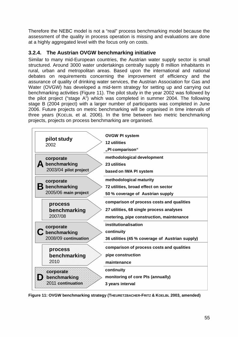
55

Therefore the NEBC model is not a “real” process benchmarking model because the assessment of the quality in process operation is missing and evaluations are done at a highly aggregated level with the focus only on costs.

3.2.4. The Austrian OVGW benchmarking initiative Similar to many mid-European countries, the Austrian water supply sector is small structured. Around 3000 water undertakings centrally supply 8 million inhabitants in rural, urban and metropolitan areas. Based upon the international and national debates on requirements concerning the improvement of efficiency and the assurance of quality of drinking water services, the Austrian Association for Gas and Water (OVGW) has developed a mid-term strategy for setting up and carrying out benchmarking activities (Figure 11). The pilot study in the year 2002 was followed by the pilot project (“stage A”) which was completed in summer 2004. The following stage B (2004 project) with a larger number of participants was completed in June 2006. Future projects on metric benchmarking will be organised in time intervals of three years (KOELBL et al. 2006). In the time between two metric benchmarking projects, projects on process benchmarking are organised.

Figure 11: OVGW benchmarking strategy (THEURETZBACHER-FRITZ & KOELBL 2003, amended)

pilot study2002

corporate benchmarking2003/04 pilot project

A

corporate benchmarking2008/09 continuation

C

corporate benchmarking 2005/06 main project

Bprocess benchmarking2007/08

36 utilities (45 % coverage of Austrian supply)continuityinstitutionalisation

metering, pipe construction, maintenance

comparison of process costs and qualities

50 % coverage of Austrian supply72 utilities, broad effect on sector methodological maturity

based on IWA PI system23 utilitiesmethodological development

„PI comparison“12 utilitiesOVGW PI system

27 utilities, 68 single process analyses

process benchmarking2010 maintenance

comparison of process costs and qualities

pipe construction

D3 years intervalmonitoring of core PIs (annually)continuitycorporate

benchmarking2011 continuation

56

3.2.4.1. OVGW Corporate Benchmarking

3.2.4.1.1. Stage A (pilot project) The Austrian “Benchmarking and Best Practices of Austrian Water Supply Enterprises – Stage A” pilot project (NEUNTEUFEL et al. 2004), in which 23 water supply enterprises (from 40,000 m³ up to 140 million m³ supplied water per year) participated, was launched and conducted by OVGW and largely funded by the Austrian Ministry of Agriculture, Forestry, Environment and Water Management (BMLFUW). The OVGW commissioned three academic institutes to operationally run the pilot project from an external, objective and confidential point of view: Graz University of Technology, the Vienna University of Natural Resources and Applied Life Sciences and the Wiener Neustadt University of Applied Sciences (THEURETZBACHER-FRITZ et al. 2005). Some of the participating enterprises joined the OVGW benchmarking working group for project supervision and to incorporate practice needs into the indicator system. Thus, the OVGW system can be called a system by water suppliers for water suppliers. The co-operation with the Bavarian (Germany) EffWB project (KIESL & SCHIELEIN 2002 and 2005), which is also based on the IWA performance indicator system, has been important for the development of the OVGW system. Due to the similar water supply structure of Austria and Bavaria, a cross border co-operation was defined to develop a compatible system and to conduct trans-national comparisons. The Bavarian-Austrian co-operation can be seen as an innovative application and further development of the IWA system generating the chance of large participation (200 participants and more) in these benchmarking activities (THEURETZBACHER-FRITZ et al. 2005). The main aim of the pilot project was to implement a benchmarking system in Austria's drinking water sector in line with the following sub-objectives. The project strongly emphasises the utilisation of benchmarking for internal purposes, serving as a controlling instrument for continual improvement (“learning from the best”). It also provides public transparency of the sector’s performance and shows the sector’s free will to arrange a quasi competition, based upon the principles of voluntary and anonymous participation. A strong focus is laid on aspects of comparability (homogeneous data collection, data verification including company visits, classification of similar enterprises etc.), on a holistic approach (according to the IWA performance indicator system, ALEGRE et al. 2000) and on data security and confidentiality. Based on the five-columns-model (compare HIRNER & MERKEL 2002, Figure 12), the OVGW corporate benchmarking system is a holistic system considering the five target categories supply safety, supply quality, customer service, sustainability and efficiency but also the task fulfilment, outsourcing and organisation. The OVGW pilot project system consists of 120 performance indicators calculated from 150 variables. In addition to these variables, 100 questions about task fulfilment and outsourcing, 80 questions about organisation and 150 facts as background information for high comparability complete the system. Although the aim of a working benchmarking system was reached, a need for an optimisation of this system was seen before starting the next stage.

57

Figure 12: Target categories of OVGW benchmarking system (HIRNER & MERKEL 2002, amended, in NEUNTEUFEL et al. 2004)

3.2.4.1.2. Stage B (2004 project) The aim of the 2004 project was the further improvement and the use of the system to achieve a broad effect on the water sector. One of the main improvements was the reduction of the number of performance indicators to 75 performance indicators instead of 120 and the concentration on 90 facts as background information instead of 150. To benchmark the level of customer services 30 questions concerning three different topics were defined (“Service Quality”, “Tariffs & Billing”, “Customer Information & Relationship”). Other innovations which are not covered by the current IWA PI system (ALEGRE et al. 2006) are an “Average Network Age Index” (NEUNTEUFEL et al. 2007), which takes life-cycles of material groups into account and is used for comparisons of rehabilitation rates, water losses and failure rates. Also the “ILI - Infrastructure Leakage Index”, a very important water loss PI, was implemented in the OVGW Benchmarking system. A homogeneous collection of personnel figures is crucial for comparable results. Besides outsourcing of tasks to external organisations, the fulfilment of tasks by overhead service units is taken into consideration. Water utilities in Austria are either embedded in larger organisations like city works and municipal administrations or have to fulfil their tasks “stand-alone” like water co-operations and water co-operatives. Therefore an index value for in-house outsourcing was developed in order to confine the employees of the water supply unit from overhead units and to better assess PIs like personnel costs and outsourcing costs (THEURETZBACHER-FRITZ et al. 2007). With a respectable amount of 72 water supply enterprises participating in the OVGW 2004 project, a high representativeness is given (about 332 million m³ water intake per year or about 50 % of water supplied in Austria). The Austrian experience shows that voluntary and anonymous participation is an essential precondition for motivated participants and, therefore, good data quality. Company visits by the project team also proved to be necessary for the project success.

58

The results of this corporate benchmarking project were published in two reports, one individually for each company and a public report (THEURETZBACHER-FRITZ et al. 2006) and are not discussed within this work. Generally speaking, the results confirm the high quality and efficiency of the Austrian water supply sector even if there are potentials for improvements.

3.2.4.2. OVGW Process Benchmarking 2007 As in other countries, process benchmarking is seen in Austria as the logical continuation and complement of the accomplished corporate benchmarking. Therefore the OVGW started its process benchmarking initiative in 2006. The aim of the OVGW process benchmarking is a comparative analysis and the optimisation of different working processes of water undertakings. The frame conditions of the OVGW process benchmarking are similar to the OVGW corporate benchmarking:

• The Austrian benchmarking is a voluntary and anonymous comparison of company performances.

• The project is conducted by the OVGW (Austrian Association for Gas and Water). The OVGW in the rule of project executing organisation is the strategic project coordinator and represents the interests of water undertakings.

• Strong focus is put on data security and data confidentiality. All company-data are governed and interpreted confidentially by a neutral and objective project team.

• The project team consists of two academic institutes: Graz University of Technology, Institute of Urban Water Management and Water Landscape Engineering and the Vienna University of Natural Resources Applied Life Sciences - Institute of Sanitary Engineering and Water Pollution Control.

• The Austrian system of process benchmarking was developed by the project team, which works closely with water suppliers. This approach was also successful in the corporate benchmarking project and enables practical applicability.

• The OVGW process benchmarking system is a modular system. Therefore it is not necessary to participate in all the processes.

• Participants have to pay a participation fee, depending on the size of the water company and the complexity of the analysed process.

• It is important that the effort for data collection is in due proportion to the benefits expected. Therefore process analyses are based on characteristic random samples.

Based upon a best practice approach, the results of the comparison are discussed in workshops. Thus, the participants can exchange experiences and derive measures for improvements of each process (KOELBL et al. 2007a). The OVGW process benchmarking focuses on three subject areas. In the first attempt, six of the eight offered processes were analysed (Table 8). Depending on companies needs, others can follow.

59

Table 8: Processes of OVGW process benchmarking 2007

Sales Process Customer meter reading

Customer meter replacement

Construction of pipes

Construction of new mains

Construction of new service connection (not realised)

Rehabilitation of mains

Rehabilitation of service connections

Mains network operation and maintenance

Water loss management

Network inspection (not realised) The following sub-chapters give a short overview about the single processes.

3.2.4.2.1. Process 1: Customer meter reading The aim of benchmarking this process is to analyse all the activities for customer meter reading and billing regarding costs and quality of execution. A specific challenge in benchmarking customer meter reading is the evaluation of three possible variants in process operation: meter reading by water supply utility personnel (variant 1), reading by customers (variant 2) and remote meter reading (RMR, variant 3). The process structures of the different variants are shown in Figure 13.

Figure 13: Process structure of customer meter reading (KOELBL et al. 2008b)

Depending on the variants, the process includes customer information about the meter reading (fixing a date), the meter reading itself (by water company personnel or outsourced personnel, by customer or with remote meter reading) but also additional meter readings and processing of meter readings by customers (postcards, online data management). Furthermore, accounting and debtor management are analysed. The aim is the comparison of different meter reading and accounting methods in order to find an optimal (most efficient) approach for each company, depending on individual frame conditions (KOELBL et al. 2008b).

preparation meter reading billing

q u a l i t y o f p r o c e s s o p e r a t i o n

- invoicing- debtor management- accounting

costs, time costs, timecosts, time

variant 2reading by customer

variant 1personnel of water utility

variant 3remote meter

reading

- planning meter reading

- customer information- personnel organisation

- customer information

- planning meter reading

- personnel organisation

- travel- meter reading- evaluation

- evaluation

- travel- meter reading- evaluation

- invoicing- debtor management- accounting

60

3.2.4.2.2. Process 2: Customer meter replacement To benchmark this process, all the activities for routine meter replacements (in accordance with Austrian law every 5 years) are analysed. The first step is customer information and fixing a date (by postcard or telephone call). Changing meters can be done by water utility personnel or by external companies. But the management of customer meters and storage or disposals of used meters is also part of this process (see Figure 14). To avoid a comparison of apples with oranges, three different variants have to be considered: replacement of conventional meters, replacement of remote meters and installation of new remote meters (KOELBL et al. 2008b).

Figure 14: Process structure of customer meter replacement (KOELBL et al. 2008b)

3.2.4.2.3. Process 3: Construction of new mains All the activities and costs for constructing new mains are analysed in this process. The first steps of this process are the planning and tender processes (e.g. done by a civil engineer). After the awarding of a contract, the construction process follows. One aim is the evaluation of costs per meter mains dependent on different frame conditions (open land or city) and different materials and diameters. For costing it does not matter whether the construction is done by company personnel or by external companies (often digging and rebuilding of streets is done by external companies whereas piping is done by personnel of the water undertakings). The documentation of constructed mains in maps and GIS (geographic information systems) and in accounting is also part of the process.

3.2.4.2.4. Process 4: Construction of new service connections (Note: not realised in the 2007 project due to less participants) All the activities and costs for constructing new service connections are analysed in this process. The process starts with customer information and fixing a date. Next, the water undertaking builds the service connection or connects the pipe (which was laid by the customer) to the main and installs the meter at the end of the service connection. The last steps are the documentation of service connections in maps and GIS (geographic information systems) and in the accounting system.

3.2.4.2.5. Process 5: Rehabilitation of mains The process starts with rehabilitation planning and determining mid-term and long-term rehabilitation measures. The experiences have shown that this step is done in many different ways. Whereas larger water undertakings use IT-based programs which work on the basis of failure statistics, smaller companies often act “on personal experience” or in correlation with other constructions (for example gas pipes or

preparation meter replacement additional activities

q u a l i t y o f p r o c e s s o p e r a t i o n

- internal organisation- purchase or gauging of

meters- time scheduling- customer information

- preparation of replacement- travel- meter replacement- other services

- customer meter management- internal optimisations- storage or disposal

costs, time costs, time costs, time

61

sewers) by defining which pipes to be renewed. The next steps are similar to process 3 (Construction of new mains). After analysing costs for planning and the tender process, the costs per meter mains dependent on different frame conditions (open land or city) and different materials and diameters and different methods (for example new pipe or relining) are evaluated. But the documentation of rehabilitated mains in maps and GIS (geographic information systems) and in accounting systems is also part of the process.

3.2.4.2.6. Process 6: Rehabilitation of service connections In this process all the activities and costs for rehabilitation of service connections are analysed. The process starts with rehabilitation planning and determining mid-term and long-term rehabilitation measures for service connections. Rehabilitations of service connections often occur simultaneously with mains rehabilitation, but also in separated programs (for example replacement of lead pipes). In addition to planning and construction, the documentation of rehabilitated service connections in maps and GIS (geographic information systems) and in the accounting system is also analysed.

3.2.4.2.7. Process 7: Water loss management The process of water loss management probably represents one of the most complex processes within the OVGW 2007 project. The process of physical water management is a highly integrative process which is influenced by many single tasks of almost all the operating duties of a water supply utility (see chapter 5). The objectives of benchmarking the process of water loss management are qualitative and quantitative comparisons of different strategies and methodologies in water loss management (leakage monitoring, leak detection). Thereby not only different methods with the associated costs but also the success of these methods are analysed. The calculation of the IWA water balance is necessary as a basis for the process comparison, and one aspect is the accuracy of water balance. Chapter 6 describes the results and experiences of benchmarking the process of water loss management within the 2007 OVGW process benchmarking.

3.2.4.2.8. Process 8: Network inspection (Note: not realised in the 2007 project due to less participants) Network inspections are preventative and routine measures (for example visual checkups on the existence and readability of warning and information signs, functional checks of valves, hydrants etc., status checks of shafts or smaller maintenance like cleaning or lubricating). The activities analysed are adapted to the ÖNORM B 2539 - OVGW W 59 guideline (2005). The process starts with the planning of inspection and maintenance activities on basis of a network analysis. Besides the activities of inspection, the management of these activities within a database for planning future measures is also part of this process. Not only the activities themselves but also the associated costs are analysed.

62

4. Basics of Water Loss Management Within the last two decades many developments in the sector of water loss management have been made. Many of these developments have been driven by problems with water losses in developing countries, which in general have much higher water losses in their water supply systems than networks in central Europe like those in Austria, Germany or Switzerland. Experts from the UK, where the water infrastructure is often in a worse condition in comparison to Austria, or from countries with limited resources like Australia or Cyprus have made especially substantial contributions. But some Austrian experts are also very active in the international water loss scene. Since 1996 a separate task force within the IWA Efficient Operation and Management of Urban Water Distribution Systems Specialist Group has been dealing with this topic – the Water Loss Task Force (WLTF). The aim of this group is to bring experts from all over the world together to develop effective and sustainable international “best practises” in the management of water losses. A main concern of the WLTF is sharing information with a broad user stratum (especially water supply utilities in developing countries). Therefore many publications, e.g. guidelines, are free available from the WLTF website. Other important information platforms are the Specialist Conferences which are organised biannually. In September 2007 the Water Loss 2007 took place in Bucharest (Romania) and before this there were conferences in Halifax (Canada, 2005) and Lemesos (Cyprus, 2002). One of the first important duties of the WLTF was to work out a consistent terminology, a standardised water balance and various performance indicators for the comparison of water losses. In 2000 the IWA Blue Pages of “Losses in Water Supply Systems” were published (LAMBERT & HIRNER 2000). The terminology, the water balance and the performance indicators described in the Blue Pages were implemented to the IWA “Performance Indicators for Water Supply Services” Manual of Best Practices (ALEGRE et al. 2000 and 2006). A short overview about the most important aspects of the IWA methodology in water loss management and the earliest developments in this field is given in the following pages. References to the DVGW W 392 (2003) German standard – “Network inspections and water losses – activities, procedures and assessment” and several Austrian standards are made.

4.1. Why Water Loss Management? Unlike the situation in countries with high water losses, it seems to be quite unattractive to undertake extensive water loss management for a typical Austrian water utility. Often the water production costs are very low in cases no treatment is necessary. Many Austrian water works are in the lucky situation that a high amount of their water does not have to be pumped (e.g. natural springs with gravitation pipes) and therefore also the costs for distributing the water can be very low. The installation of leakage monitoring systems and leak detection are expensive and time consuming. The repair of leaks is expensive, too. So if the costs of lost water are compared with the effort for the minimisation of leakage only from an economic point of view, water loss management does not seem to make sense for many Austrian water supply utilities.

63

But beside these economic aspects there are many reasons to keep the level of water losses low. In the OVGW W 63 Austrian standard (1993 and in press) – “Water Losses in Water Supply Systems” and in DVGW W 392 (2003), the following aspects are described:

• hygienic aspects o each leak represents a risk of contamination by entering water from

outside in the distribution system (e.g. in case of pressure decline)

• aspects of supply techniques and supply safety o leakage can lead to quantitative problems (e.g. in situations of peak

supply) o leakage can cause decrease of service pressure and can lead to

customer complaints

• ecological aspects o water losses contravene recent ecological concepts o low water losses reduce the energy demand of pumps, treatment

stations etc. and reduce therefore the CO2 emissions o low water losses help saving resources

• economic aspects o in general high water losses cause higher running costs (e.g. energy

costs, treatment chemicals, higher maintenance costs) o low water losses prevent (or postpone) the exploitation of new

resources It is stated in DVGW W 392 (2003) that economical aspects only play a role at high levels of water losses. This strategy is completely different from that of the privatised English water sector, where economic aspects are most relevant (compare LIEMBERGER 2005). The OVGW W 100 Austrian directive (2007) – “Water supply pipes – operation and maintenance” also urges for low leakage levels. Furthermore, in DVGW W 392 (2003) the importance of low water loss levels as decisive indicator for the condition of the pipe network and the fact that low water losses lead to a reduced effort for the maintenance of the pipe network are described. Therefore the calculation of water loss PIs not only for the whole water supply system but also for single network zones provides important information about the condition of the pipe network. This information is essential for an effective maintenance and rehabilitation planning and shows the importance of water loss management even in water supply systems with low leakage levels. Beside these technical criteria legal aspects are also relevant e.g. claims for indemnification after settlements in consequence of washouts.

4.2. IWA Blue Pages – definitions and standardised water balance The objectives of the “Losses from Water Supply Systems: Standard Terminology and Recommended Performance Measures” IWA Blue Pages (LAMBERT & HIRNER 2000) are to prepare a recommendation for a basic standard terminology for the

64

calculation of real and apparent losses and to recommend preferred performance indicators of water losses for international comparisons.

Figure 15: Definition of water supply system inputs and outputs (LAMBERT & HIRNER 2000)

Water intake

Raw water mains

Treatment

Transmission

Storage

Distribution

Imported raw water (*)

Exported raw water (*)

Imported treatedwater (**)

Exported treatedwater (**)

Water abstracted

Treatment input

Water produced

Transmission input

Distribution input

Water supplied

Raw water consumptionand losses

Treatment, operational consumption and losses

Transmission, consumptionand losses

Storage tanks, operational consumption and losses

Distribution, consumptionand losses

Meter

District

metering

(*) –can

belocated

anywhere

between

thew

aterintakeand

thetreatm

ent(**) –

canbe

locatedanyw

heredow

nstreamtreatm

ent

65

According to LAMBERT & HIRNER (2000), reliable metering of all water volumes should and must be an integral component of the water supply, water demand management and loss determination. The most important part of determining how much water is being lost in a system is to accurately quantify the volume of water which is entering that system. Metering of source meters for abstraction, treatment works production, imported and exported water, input volumes and inflows to sectorised distribution systems is essential for water balance calculations (Figure 15). The DVGW W 392 (2003) also claims that exact definitions of all components of a water balance are a precondition for discussions about water losses. It is also mentioned that all the inputs and outputs of a water supply system need to be measured. ALEGRE et al. (2006) describe following definitions:

Water abstracted: the volume of water obtained for input to water treatment plants (or directly to the transmission and distribution systems) that was abstracted from raw water sources during the assessment period.

Raw water, imported or exported: the volume of bulk transfers of raw water across operational boundaries during the assessment period. The transfer can occur anywhere between the abstraction point and the treatment plant.

Treatment input: the volume of raw water input to treatment works during the assessment period.

Water produced: the volume of water treated for input to water transmission lines or directly to the distribution system during the assessment period. (The volume of water that is distributed to consumers without previous treatment shall be also accounted for in water produced).

Treated water, imported or exported: the volume of bulk transfers of treated water across operational boundaries during the assessment period. The transfer can occur anywhere downstream treatment. (The volume of water – if any – that is abstracted and delivered to consumers without any treatment shall be also accounted for as treated water in scope of the water balance).

Transmission input: the volume of treated water input to a transmission system during the assessment period.

Distribution input: the volume of treated water input to a distribution system during the assessment period.

Supplied water: the distribution input minus treated water exported. (When it is not possible to separate transmission from distribution, supplied water is the transmission input minus treated water exported).

System input: the volume input to water supply system during the assessment period.

Authorised consumption: the volume of metered and/ or non-metered water taken by registered customers, the water supplier and others who are implicitly or explicitly authorised to do so by the water supplier, for residential, commercial and industrial purposes, during the assessment period. It includes water exported. (Note: Authorised consumption may

66

include items such as fire fighting and training, flushing of mains and sewers, street cleaning, watering of municipal gardens, public fountains, frost protection, building water, etc. These may be billed or unbilled, metered or unmetered, according to local practice. Authorised consumption also includes leakage and waste by registered customers that are unmetered.).

Real losses: physical water losses from the pressured system, up to the point of measurement of customer use during the assessment period. The volume lost through all types of leaks, bursts and overflows depends on frequencies, flow rates and average duration of individual leaks. (Note: Although physical losses after the point of customer flow measurement are excluded from the assessment of real losses, they are often significant - particularly where customers are unmetered – and worthy of attention for demand management purposes.).

Apparent losses: accounts for all types of inaccuracies associated with production metering and customer metering, plus unauthorised consumption (theft or illegal use). (Note: Under-registration of production meters, and over-registration of customer meters, leads to under-estimation of real losses and the opposite way around.).

Non-revenue water: the difference between the volumes of system input and billed authorised consumption. Non-revenue water includes not only the real losses and apparent losses, but also the unbilled authorised consumption.

Table 9: Components of IWA water balance (LAMBERT & HIRNER 2000)

Note: All parameters in m³ per year (m³/year)

Based on these system definitions a standardised water balance is described within the IWA Blue Pages (Table 9). Meanwhile, this type of water balance described by IWA is being used in many countries all over the world, e.g., Australia, Germany, Canada, New Zealand, South Africa and by the American Water Works Association (LIEMBERGER 2006). It was implemented into the IWA PI-system (ALEGRE et al. 2006)

Apparent Losses

Real Losses

(= Physical Losses)

Leakage on Transmission and/or Distribution Mains

Leakage and Overflows at Utility`s Storage Tanks

System Input Volume

Revenue Water

Non-revenue Water

Water Losses

Authorised Consumption

Leakage on Service Connections up to Point of Customer Metering

Billed Authorised

Consumption

Unbilled Authorised

Consumption

Billed Metered Consumption

Billed Unmetered Consumption

Unbilled Metered Consumption

Unbilled Unmetered Consumption

Unauthorised Consumption

Customer Metering Inaccuracies

67

and also into the DVGW W 392 worksheet of the German Association for Gas and Water, which is the valid standard for German water utilities. The Austrian Association for Gas and Water uses also this system within the OVGW benchmarking project (compare NEUNTEUFEL et al. 2004) and it is implemented in the new OVGW W 63 directive (in press). An exact metering of the system input and the authorised consumption are essential for a meaningful water balance. Inexact metering leads to an inexact result and the amount of physical losses can then be over or under estimated (compare DVGW W 392, 2003). Therefore LAMBERT & HIRNER (2000) point out the importance of an accurate metering of the system input but also of consumption. Another important point for calculating a water balance is the determination of “unbilled unmetered consumption”, e.g. water for fire fighting, washing streets or public gardening. These consumptions are often not metered and in many cases not documented. So a special focus should be laid on training how to meter and document the unbilled consumption. To confine the system input correctly it is necessary to deduct “returned water” from the system input (see Table 10). For the water supply sector “returned water” can be defined as water that is consciously taken from the water supply system at another point than before the system input (e.g. spring collection shafts), e.g. unused water that is abstracted of reservoirs or water used for producing electricity at drinking water power stations, which are very common in the alpine regions of Austria. The points of water abstraction can be situated in the transport or the distribution system. This definition must not be mistaken for “returned water” as defined by NAGY et al. (2007) for the OECD/Eurostat Joint Questionnaire on Inland Waters where returned water is water abstracted from any fresh water source and discharged into fresh waters without use, or before use. This occurs primarily during mining and construction activities. Discharges to the sea are excluded.

Table 10: Water balance including consideration of returned water

Returned Water

Water Losses before Treatment

Abstracted Water

System Input Volume

Authorised Consumption

Unbilled Authorised

Consumption

Unbilled Metered Consumption

Non-revenue Water

Unbilled Unmetered Consumption

Billed Authorised

Consumption

Billed Metered ConsumptionRevenue

WaterBilled Unmetered Consumption

Water Losses

Apparent Losses

Unauthorised Consumption

Customer Metering Inaccuracies

Real Losses

(= Physical Losses)

Leakage on Transmission and/or Distribution Mains

Leakage and Overflows at Utility`s Storage Tanks

Leakage on Service Connections up to Point of Customer Metering

68

4.3. Four basic methods for managing physical water losses Beside other publications on this topic, FARLEY & TROW (2003) describe the IWA methodology in water loss management very clearly. Figure 16 shows an overview of the basic correlations. The white rectangle in Figure 16 represents the unavoidable annual real losses (UARL). These are losses which usually can not be prevented even with an optimal water loss management system. The surrounding grey rectangle represents potentially recoverable physical (= real) water losses. These potential savings change with the strength of the arrows acting on this square. The double arrow (pressure management) above the square indicates that the water losses decrease by reducing the service pressure and also the other way round. The burst frequency can also be decreased significantly with pressure reduction (see chapter 4.6). There are also many international examples for high savings of water through temporary pressure reduction over the night hours (e.g. MCKENZIE et al. 2007).

Figure 16: The four basic methods for managing physical water losses (FARLEY & TROW 2003, amended)

The type and extent of leakage control are very important for the amount of water losses. The term Active Leakage Control includes not only measures of leakage detection (e.g. step testing, common sounding surveys, noise logging or gas checks) but also measures of leakage monitoring. This means monitoring the system input and also single zones or DMAs (District Metered Areas) and managing all the technical equipment for these measurements (see chapter 4.5). Depending on the existing technical equipment of a water supply utility, two different strategies in leakage detection are possible:

• “cause based” leak detection or • leak detection “on rotational basis” (in fixed intervals, e.g. annual leak

detection campaigns without a concrete guess for failures). Infrastructure management covers various tasks which directly or indirectly influence the amount of water losses. Beside the technical equipment of a water

speed and quality of repair

active leakage control

pressure manage-

ment

infra-structure manage-

ment

UARL

potentially recoverable

physical losses

69

supply utility, the rehabilitation management (including analyses of pipe group based failure statistics), the management of maintenance (fittings, pumps, flow meters, valves etc.) but also the customer meter management (average age of customer meters, methodology of meter reading etc.) and hydraulic modelling of the supply system are part of this topic. In general, infrastructure management covers long-term measures which can not be influenced over short time periods. The speed and quality of repair is also essential for the amount of water losses. The repair time is the time taken from locating a leak to the recovery of the functionality of the pipe. The amount of water lost at a single leak is calculated by the product of the flow rate and the run time of the leak. Formula 1: Calculation of volume lost

volume lost (m³ or l) = flow rate (m³/d or l/h) x run time (d or h)

For the total volume lost at leaks this means that small leaks, which are often not recognised by leakage monitoring and therefore have a long run time, might lead to high water losses (Figure 17). Unreported leaks which are found in the course of leak detection campaigns (subject to interval and methodology) often have middle flow rates and lead to middle or high losses. On the other hand, reported leaks usually have high flow rates but due to a short run time the total volumes of losses are relatively small.

Figure 17: Effect of burst duration on total leakage (MORRISON et al. 2007)

It also has to be mentioned that one of the most important criteria in water loss management is the qualification of the staff. All the tasks described in this chapter (pressure management, active leakage control, infrastructure management or repair of leaks) require well trained, motivated and experienced personnel to achieve success.

run time

run time

flow

rate

3 days 2 days 1 day

distribution main burst with flow rate of 4 m³/h

awareness location repair

total run time of leak = 6 days

total loss of water = 576 m³

flow

rate

60 days 14 days 1 day

service pipe leak with flow rate of 0.4 m³/h

awareness location repair

total run time of leak = 75 days

total loss of water = 720 m³

70

4.4. Quantification of Water Losses with Performance Indicators Defined performance indicators (PIs) are required to quantify the amount of water losses in order to compare them for internal purposes (e.g. monitoring the development of leakage or comparison of different DMAs) or external purposes (comparison with other water utilities). One problem in the use of PIs is the influence of frame conditions of different water supply systems. Different PIs favour or penalise certain structures. Therefore it is very important to consider the frame conditions of the utilities compared (e.g. KOELBL et al. 2007b). The most important influencing factors on the amount of water losses are:

• the structure of the distribution system (the urbanity – rural, small city or large city; note: within the OVGW benchmarking system the urbanity considers the network delivery rate, the service connection density and the consumption per customer meter, compare NEUNTEUFEL et al. 2004),

• the condition of the water supply network (proportion, age and condition of single pipe groups),

• the average service pressure but also

• the soil conditions (compare DVGW W 392, 2003). The following discussion of various water loss PIs should help finding out the appropriate PIs for the comparisons of water losses. The following PIs are discussed:

• water loss ratio (%)

• real losses per mains length (m³/km·h)

• real losses per connection and day (l/conn·d)

• real losses per connection and day per metre service pressure (l/conn·d·m)

• Infrastructure Leakage Index

• non-revenue-water (%),(m³/km·h) or (l/conn·d)

4.4.1. Water Loss Ratio (%) The water loss ratio represents the percentages of the real losses related to the system input. This PI is still very common although it is definitely unsuitable for the assessment of water losses (compare LAMBERT & HIRNER 2000 or DVGW W 392, 2003). Formula 2: Water loss ratio

)/³(100*)/³((%)aminputsystemannual

amlossesrealannualratiolosswater =

This performance indicator should only act as a first reference value for discussing water losses. This PI is insufficient for a technical interpretation of water losses because the structure of the supply system (length of mains, number of service connections etc.) is not considered. Furthermore, within the calculation there is a division by the system input, a value that changes every year depending on the weather conditions but also from the consumption of large consumers (industry). So it is possible that the actual losses of a certain year are higher than those of another

71

year whereas the water loss ratio is smaller because the system input and the consumption have also increased (see example in Table 11).

Table 11: Example of a comparison of water loss ratios for two years

year 1 year 2

system input 1,400.000 m³ 1,000.000 m³

consumption (households) 880.000 m³ 880.000 m³

consumption (industry) 385.000 m³ 0 m³ (industry closed)

apparent losses 20.000 m³ 20.000 m³

real losses 115.000 m³ 100.000 m³

water loss ratio 8 % 10 %

4.4.2. Real Losses per Mains Length (m³/km·h) Unlike the water loss ratio this PI has the advantage that the structure of the supply system is considered with the total mains length. The mains length is a more or less statically denominator. Therefore this PI can be used to watch the development of water losses within a supply system or a single DMA. Formula 3: Real losses per mains length

)/(8760)()/³()·/³(

ahxkmlengthmainstotalamlossesrealannualhkmmlengthmainsperlossesreal =

In DVGW W 392 (2003) the real losses per mains length are the decisive PI and assessments in subject to the structure of the distribution network (rural, urban or metropolitan) can be done (see Table 12; note: in contrast to the OVGW benchmarking system DVGW W 392 classifies the structure of a water supply system on basis of the network system input rate).

Table 12: Standard values for real water losses per mains length in water distribution networks in m³/km·h according to DVGW W 392 (2003)

assessment of water losses

structure of distribution network

area 1 (metropolitan)spec. network

system input rate >15.000 m³/km·a

area 2 (urban) spec. network

system input rate 5.000-15.000

m³/km·a

area 3 (rural) spec. network

system input rate <5.000 m³/km·a

low water losses < 0.10 < 0.07 < 0.05

medium water losses 0.10 - 0.20 0.07 - 0.15 0.05 - 0.10

high water losses > 0.20 > 0.15 > 0.10

The differentiated classification scheme of DVGW W 392 (2003) determines that comparisons of this PI are only allowed within a group of comparable and similar structured water utilities. The real losses per mains length of a rural water utility cannot be compared with those of a metropolitan one. The IWA Water Loss Task Force (WLTF) criticises the decision of DVGW to select this indicator as the decisive PI because experience shows that the majority of water losses usually appear at service connections. Therefore the PI “real losses per

72

connection and day” described below should have been preferred (compare LIEMBERGER 2005, LAMBERT et al. 1999 and LAMBERT & HIRNER 2000). Nevertheless, the WLTF (LIEMBERGER 2007) and also ALEGRE et al. (2006) recommend using this PI for supply systems with service connection densities smaller than 20 per kilometre.

4.4.3. Real Losses per Connection per Day (l/conn·d) The main origins of water losses are considered with the number of service connections. Formula 4: Real losses per connection and day

)/(365)/³()·./³(

adxsconnectionserviceofnumberamlossesrealannualdconnmdayperconnectionperlossesreal =

Concerning the comparability of this PI, similar constraints to those for real losses per mains length have to be made. So comparisons have to be done within a group of supply systems with the same structure. The IWA, WLTF (LIEMBERGER 2007) and also ALEGRE et al. (2006) recommend using this PI for supply systems with service connection densities higher than 20 per kilometre.

4.4.4. Real Losses per Connection per Day per Metre Service Pressure Head (l/conn·d·m)

Beside the service connection density this PI considers the average service pressure. The average service pressure head is a very important parameter because the flow rate of leaks is mainly influenced by the pressure. Formula 5: Real losses per connection and day per metre service pressure head

)(..)/(365...1000)/³(......

mheadpressserviceavxadxconnservofnbxamlossesrealannualheadpressservpdaypconnplossesreal =

Up to now the use of this PI has not been very common in Austria.

4.4.5. Infrastructure Leakage Index (ILI) Compared to other water loss PIs like “real losses per mains length” or “real losses per connection and day”, the Infrastructure Leakage Index (ILI) also includes essential influencing factors like the average network pressure and the service connection density as well as the mains length and the length of service connections (Formula 6). Therefore the ILI is the only PI that enables performance comparisons of different structured water supply systems. To calculate the ILI the Current Annual Real Losses (CARL) are divided by the so-called Unavoidable Annual Real Losses (UARL). The ILI indicates the multiple by which the real losses are higher than the unavoidable annual real losses. The unavoidable annual real losses are a theoretical (reference) value which was developed and calibrated by the IWA WLTF on basis of statistical analysis of international data, including 27 different water supply systems in 20 countries (LAMBERT & HIRNER 2000). The ILI is also part of the IWA PI system (ALEGRE et al. 2006).

73

Formula 6: ILI – Infrastructure Leakage Index

ILI = CARL / UARL CARL = Current Annual Real Losses (litre/connection·day)

UARL = Unavoidable Annual Real Losses (litre/connection·day)

Formula 7: UARL – Unavoidable Annual Real Losses

PLpNcLmUARL ×⎟

⎠⎞

⎜⎝⎛ ×++×= 025,08,018

Lm = length of mains (km)

Nc = number of service connections

Lp = average length of service connections from property boundary to measurement point (m)

P = metre of average service pressure (m)

Even if, on the first view, ILI represents a quite complex indicator, this PI has been implemented for water loss calculations in many countries all over the world. International experiences show that the calculation of this indicator works quite well and therefore also cross-border comparisons are possible without further groupings (e.g. urbanity). In the Austrian drinking water sector this PI was not common until the beginning of the OVGW benchmarking activities. First the ILI was implemented into the OVGW benchmarking system for the purpose of testing. Experiences with ILI within the OVGW benchmarking are almost all positive, even if this highly aggregated indicator seems to be too complex for some participants in the first instance (THEURETZ-BACHER-FRITZ et al. 2006 and KOELBL et al. 2007b). However there are some limitations on applying the UARL formula. Originally the equation should not have been used for systems with less than 5000 service connections, less than 20 connections per km of mains, and less than 25 metres of service pressure head (LAMBERT & MCKENZIE 2002). On the basis of the following research, the lower limits for number of service connections have been reduced to 3000 and the lower limit on the density of service connections has been removed. The lower limit of 25 metres for pressure was introduced to avoid significant errors from extrapolating the assumption of a linear pressure : leakage relationship to systems with 100 % flexible pipes at low pressures, where the N1 exponent would be close to 1.5 (note: leakage varies with pressureN1, compare Formula 11 in chapter 4.6), (LIEMBERGER & MCKENZIE 2005). Recent experiences with the calculation of ILIs show that lower limits for the number of service connections are not necessary in developed countries. GANGL & KOELBL (2009) describe the relationship between ILI and real losses per mains length for 34 Austrian water utilities, which participated in the OVGW corporate benchmarking 2008 (data of 2007). Figure 18 shows the maximal possible values for ILI and real losses per mains length. These values consider the possible error margins for real losses and for the mains’ length. Therefore, the values shown are probably a little bit too high; in fact the “true value” for each utility has to be anywhere between the value calculated directly from the variables and the maximum possible value. But this aspect is irrelevant for the purpose of showing that there is a good correlation of these two PIs and that no influence of the system size is evident.

74

Figure 18: Comparison of maximal possible values of ILI with real losses per mains length (GANGL & KOELBL 2009; data source: OVGW benchmarking 2008 – stage C)

The same is valid for the correlation between ILI and real losses per connection per day (Figure 19).

Figure 19: Comparison of maximal possible values of ILI with real losses per connection per day (data source: OVGW corporate benchmarking 2008 – stage C)

Because practical experiences show that it is possible (under special frame conditions, e.g., no unreported leaks, young network) to achieve ILI values smaller than 1.0 (note: values down to 0.7 are known, compare LAMBERT, in press; e.g. for very well managed systems in Australia and in Austria), it is discussed to rename the

0.0

0.1

0.2

0.3

0.4

0.5

0.6

0.7

0.8

0 1 2 3 4 5 6 7 8 9 10 11 12

ILI

real lo

sses per m

ains leng

th (m

³/km

.h)

<3000 service connections >3000 service connections

0

200

400

600

800

1000

1200

0 1 2 3 4 5 6 7 8 9 10 11 12

ILI

real lo

sses per con

nection pe

r da

y(l/conn

.d)

<3000 service connections >3000 service connections

75

UARL from “unavoidable annual real losses” to any kind of reference value (note: the World Bank Institute uses the term “Minimal Achievable Annual Physical Losses”, MAAPL). The results of the 2008 OVGW corporate benchmarking show that even under consideration of all possible error margins for single water balance and supply system data some of the utilities have ILIs under 1 (Figure 18). Such an adaptation of the UARL definition might increase the acceptance of the ILI in developed countries where the water supply systems are in a very good condition. But it also has to be mentioned, that recent investigations show, that small ILI values are often a result of inappropriate water balance data. When the real losses are very low, systematic failures (e.g. accuracy of system input meters) in the water balance can lead to large possible error margins. LAMBERT (in press) agrees that “unavoidable” is not a precisely accurate term when applied to annual real losses (UARL) but it has its merits of simplicity and is well established after 10 years of use. Therefore a change in the terminology might lead to more confusion than the original term “unavoidable annual real losses”. It also has to be mentioned that the calculation of ILIs for water supply systems with very low service pressure and / or intermittent supply (e.g. in developing countries) can result in very high ILI values. So other reference values are necessary for these systems than for systems in developed countries and it does not make sense to compare such different systems with each other (e.g. MCKENZIE et al. 2007) Meanwhile, several international standard values for ILI have become available. Table 13 gives an overview of Australian ILI standard values, which are quite rigorous in comparison to the more tolerant standard values of the American Water Works Association (AWWA) in Table 14.

Table 13: Draft version of Australian ILI standard values (LIEMBERGER 2005)

ILI Description

1,0 - 1,5 excellent

1,5 - 2,0 good

2,0 - 2,5 reasonable

2,5 - 3,0 fair

3,0 - 3,5 poor

3,5 - 4,0 unacceptable

76

Table 14: ILI standard values of AWWA (2003) in LIEMBERGER (2005)

Target ILI range

Water resources considerations

Operational considerations

Financial considerations

1 – 3

Available resources are greatly limited and are very difficult and/or

environmentally unsound to develop

Operating with system leakage above this level would require

expansion of existing infrastructure and/or

additional water resources to meet the

demand

Water resources are costly to develop or

purchase Ability to increase

revenues via water rates is greatly limited

due to regulation or low ratepayer affordability

3 – 5

Water resources are believed to be

sufficient to meet long term needs, but

demand management interventions (leakage management, water

conservation) are included in the long-

term planning

Existing infrastructure capability is sufficient

to meet long-term demand as long as reasonable leakage

management controls are in place

Water resources can be developed or

purchased at reasonable expense

Periodic water increases can be

feasibly effected and are tolerated by

customer population

5 - 8 Water resources are plentiful, reliable and

easily extracted

Superior reliability capacity and integrity

of water supply infrastructure make it relatively immune to

supply shortages

Cost to purchase of obtain/treat water is

low, as are rates charged to customers

> 8

While operational and financial considerations may allow a long-term ILI greater than 8, such a level of leakage is not an effective utilization of water

as a resource. Setting a target greater than 8 – other than as an incremental goal to a smaller long-term target – is discouraged.

< 1 Either world class performance or error in data

Table 15 shows the physical loss target matrix from the World Bank Institute`s Non-Revenue-Water training program. There is a differentiation of target values for developed and developing countries. Beside the ILI values there is also a classification scheme for real losses per connection per day for various average service pressure heads. The band for the classification of the technical performance is from A (“very good”) to D (“very poor”). The values in Table 15 are calculated for a service connection density of 40 per km and for an average length of service connections (from property boundary to measurement point) of 0 m.

77

Table 15: Physical Loss Target Matrix from World Bank Institute (in LIEMBERGER 2006)

10 m 20 m 30 m 40 m 50 m

A 1 - 2 < 50 < 75 < 100 < 125

B 2 - 4 50-100 75-150 100-200 125-250

C 4 - 8 100-200 150-300 200-400 250-500

D > 8 > 200 > 300 > 400 > 500

A 1 - 4 < 50 < 100 < 150 < 200 < 250

B 4 - 8 50-100 100-200 150-300 200-400 250-500

C 8 - 16 100-200 200-400 300-600 400-800 500-1000

D > 16 > 200 > 400 > 600 > 800 > 1000

litres/connection/day (when the system is pressurised)

at an average pressure of:de

velo

ped

coun

trie

sde

velo

ping

co

untr

ies

technical performance

categoryILI

A Further loss reduction may be uneconomic unless there are shortages; careful analyses needed to identify cost effective improvement.

B Potential for marked improvements; consider pressure management; better active leakage control practices, and better network maintenance.

C Poor leakage record; tolerable only if water is plentiful and cheap; even then analyse level and nature of leakage and intensify leakage reduction efforts.

D Horrendously inefficient use of resources; leakage reduction programs imperative and of high priority

4.4.6. Non-Revenue-Water (NRW, %, m³/km·d, l/conn·d) NRW expressed in percentages represents the portion of the system input that is not billed. According to LIEMBERGER (2007), it is absolutely necessary to subtract exported water from the system input when calculating NRW. Formula 8: NRW (%)

)/³(exp100*)/³((%)

amwaterortedannualinputsystemannualamwaterrevenuenonannualwaterrevenuenon

−−−

=−−

The IWA Water Loss Task Force disapproves of using NRW expressed in percentages as a technical indicator. This PI only can be used as financial PI, but even then it is better to compare the marginal costs of NRW with the total operational costs (LIEMBERGER 2007). For technical assessment it is necessary to calculate NRW in litre per connection per day (Formula 9) or in m³ per kilometre per day (Formula 10) because the system input (Formula 8) is not a stable denominator (LIEMBERGER 2007). This problem was also discussed for the water loss ratio in chapter 4.4.1. Formula 9: NRW (l/conn·d)

)/(3651000)/³()·/(

adxsconnectionserviceofnumberxamwaterrevenuenonannualdconnlwaterrevenuenon −−

=−−

Formula 10: NRW (m³/km·d)

)/(365)()/³()·/³(

adxkmlengthmainsamwaterrevenuenonannualdkmmwaterrevenuenon −−

=−−

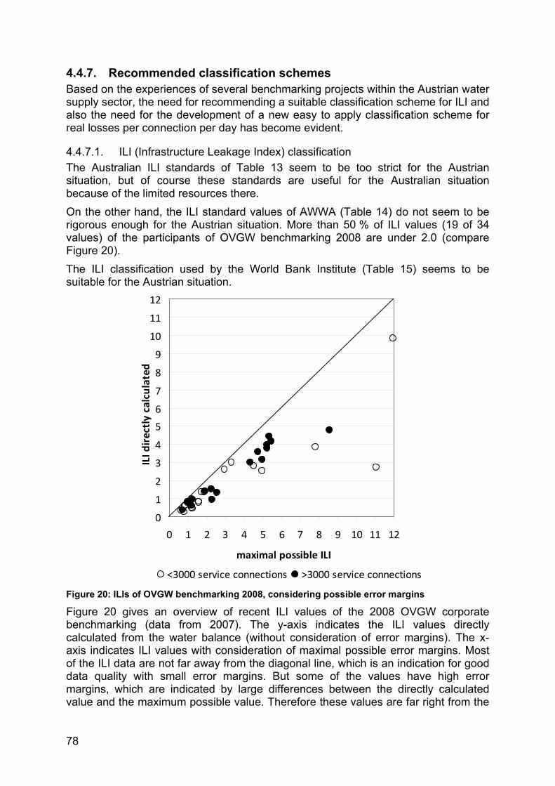
78

4.4.7. Recommended classification schemes Based on the experiences of several benchmarking projects within the Austrian water supply sector, the need for recommending a suitable classification scheme for ILI and also the need for the development of a new easy to apply classification scheme for real losses per connection per day has become evident.

4.4.7.1. ILI (Infrastructure Leakage Index) classification The Australian ILI standards of Table 13 seem to be too strict for the Austrian situation, but of course these standards are useful for the Australian situation because of the limited resources there. On the other hand, the ILI standard values of AWWA (Table 14) do not seem to be rigorous enough for the Austrian situation. More than 50 % of ILI values (19 of 34 values) of the participants of OVGW benchmarking 2008 are under 2.0 (compare Figure 20). The ILI classification used by the World Bank Institute (Table 15) seems to be suitable for the Austrian situation.

Figure 20: ILIs of OVGW benchmarking 2008, considering possible error margins

Figure 20 gives an overview of recent ILI values of the 2008 OVGW corporate benchmarking (data from 2007). The y-axis indicates the ILI values directly calculated from the water balance (without consideration of error margins). The x-axis indicates ILI values with consideration of maximal possible error margins. Most of the ILI data are not far away from the diagonal line, which is an indication for good data quality with small error margins. But some of the values have high error margins, which are indicated by large differences between the directly calculated value and the maximum possible value. Therefore these values are far right from the

0

1

2

3

4

5

6

7

8

9

10

11

12

0 1 2 3 4 5 6 7 8 9 10 11 12

maximal possible ILI

ILI d

irectly calculated

<3000 service connections >3000 service connections

79

diagonal line, e.g. the value on the lower right side with a directly calculated ILI of 2.7 and an ILI of more than 11 when considering error margins. In this special case the system input volume is not metered (estimation on basis of the delivery of springs) and therefore the error margin for real losses is very high (>400 %). Nevertheless 16 of 34 ILI values of the 2008 OVGW corporate benchmarking (data from 2007) are under 2.0 even if maximal possible error margins are considered. Therefore following ILI classification (Table 16) depending on the Physical Loss Target Matrix from World Bank Institute (Table 15) is recommended for Austria:

Table 16: Recommended ILI classification scheme (on basis of World Bank Institute)

ILI category assessment

< 2 A low water losses, further loss reduction may be uneconomic unless there are shortages

2 – 4 B medium level of water losses, potential for marked improvements, consider pressure management, better active leakage control practices and better network maintenance

4 – 8 C high level of water losses, analyse level and nature of leakage and intensify leakage reduction efforts, tolerable only if water is plentiful and cheap

> 8 D very high water losses, horrendously inefficient use of resources, leakage reduction programs imperative and of high priority

4.4.7.2. Classification for real losses per connection per day Additional to an ILI classification the Physical Loss Target Matrix of the World Bank Institute also enables a classification for real losses per connection and day depending on the average system pressure (Table 15). This matrix is calculated on basis of the ILI formula (Formula 6 and Formula 7) for the following frame conditions:

• a service connection density of 40 connections per km

• an average length of service connection of 0 m. Therefore this matrix is not applicable for all supply structures without additional calculations which would include these important frame conditions. The matrix in Table 17 was developed to enable an easy use of a classification scheme for real losses per connection and day for all utilities, depending on the average system pressure and the service connection density on basis of the ILI classification from Table 16 (categories A to D). To simplify the matrix the average length of service connections (from property boundary to measurement point) was estimated at 5 m, which represents an average value for the Austrian situation (on basis of the experiences within the OVGW benchmarking). The matrix is divided into three parts depending on the average service pressure head (20 m to 100 m). Each row of the matrix stands for a certain service connection density. To determine values for the service connection densities between two rows, an interpolation has to be done. Each of the three parts of the matrix is divided into three large columns for average service pressures. Further, each of these columns is subdivided into 4 sub-columns which indicate the categories A to D with the corresponding values for real losses per connection per day. For values between two given service pressures it is necessary to interpolate.

80

Table 17: New classification scheme for real losses per connection per day

This matrix, which is also implemented to the new OVGW W 63 Austrian directive (in press), enables a quick estimation of the water loss situation. For an exact assessment and classification it is recommended to calculate the ILI directly because the ILI formula considers exact values of pressure, service connection density and average service connection length. Figure 21 shows the application of this classification scheme described in Table 17 on the data of the 2008 OVGW corporate benchmarking. The numbers in Figure 21 indicate the average service pressure. It becomes clear that lower service pressures at the same level of real losses per connection and day lead to a worse classification, and vice versa. 19 out of the 34 data sets are classified to category “A” (low water

<110 110-220 220-435 >435 <165 165-325 325-655 >655 <220 220-435 435-870 >870

A B C D A B C D A B C D<85 85-170 170-340 >340 <130 130-255 255-510 >510 <170 170-340 340-680 >680

A B C D A B C D A B C D<75 75-145 145-290 >290 <110 110-220 220-440 >440 <145 145-290 290-585 >585

A B C D A B C D A B C D<60 60-120 120-245 >245 <90 90-185 185-365 >365 <120 120-245 245-490 >490A B C D A B C D A B C D

<55 55-110 110-220 >220 <85 85-165 165-330 >330 <110 110-220 220-440 >440A B C D A B C D A B C D

<50 50-105 105-205 >205 <75 75-155 155-310 >310 <105 105-205 205-410 >410

A B C D A B C D A B C D

<275 275-545 545-1090 >1090 <325 325-655 655-1310 >1310 <380 380-765 765-1525 >1525

A B C D A B C D A B C D<215 215-425 425-850 >850 <255 255-510 510-1020 >1020 <300 300-595 595-1190 >1190

A B C D A B C D A B C D<185 185-365 365-730 >730 <220 220-440 440-875 >875 <255 255-510 510-1020 >1020

A B C D A B C D A B C D<155 155-305 305-610 >610 <185 185-365 365-730 >730 <215 215-425 425-855 >855

A B C D A B C D A B C D<140 140-275 275-550 >550 <165 165-330 330-660 >660 <195 195-385 385-770 >770

A B C D A B C D A B C D<130 130-255 255-515 >515 <155 155-310 310-615 >615 <180 180-360 360-720 >720

A B C D A B C D A B C D

<435 435-870 870-1745 >1745 <490 490-980 980-1960 >1960 <545 545-1090 1090-2180 >2180

A B C D A B C D A B C D<340 340-680 680-1360 >1360 <385 385-765 765-1530 >1530 <425 425-850 850-1700 >1700

A B C D A B C D A B C D<290 290-585 585-1170 >1170 <330 330-655 655-1315 >1315 <365 365-730 730-1460 >1460

A B C D A B C D A B C D<245 245-490 490-975 >975 <275 275-550 550-1100 >1100 <305 305-610 610-1220 >1220

A B C D A B C D A B C D<220 220-440 440-880 >880 <250 250-495 495-990 >990 <275 275-550 550-1100 >1100

A B C D A B C D A B C D<205 205-410 410-820 >820 <230 230-465 465-925 >925 <255 255-515 515-1030 >1030

A B C D A B C D A B C D

90 m 100 m

real losses per connection per day (l/conn∙d) at an average service pressure head of

real losses per connection per day (l/conn∙d) at an average service pressure head of

real losses per connection per day (l/conn∙d) at an average service pressure head of

50 m 60 m 70 m

40

20

30

20 m 30 m 40 m

20

10

15

80 m

15

20

30

service connection

density (No./km)

50

10

40

15

Note: The calculation is based on the assumption of an average lenght of service connections (from property boundary to measurement point) of 5 m. Typical classification values for the Austrian situation are in bold letters (service connection density of 30 to 40 per km and average service pressure head of 40 to 60 m).

50

service connection

density (No./km)

30

service connection

density (No./km)

40

10

50

81

losses), 9 are in category “B” (medium level of water losses), 5 are in category “C” (high water losses) and only one utility has very high water losses (category “D”).

Figure 21: Real losses per connection per day in subject to service connection density and average service pressure (data of 2008 OVGW corporate benchmarking, data of year 2007)

There is no significant influence of the service connection density. As Figure 21 shows, very low or very high service connection densities do not result in another classification (higher or lower category). But a strong influence of the average service pressure becomes evident. On the one hand there is one utility with a very high average service pressure of 10.0 bar (real losses per connection per day: 230 l/conn·d; service connection density: 42 per km) which is classified to category “A” but has higher losses per connection per day than those utilities with lower service pressures. Therefore the average service pressure has to be considered in data interpretation. In the case of this utility a potential for reducing leakage by reducing the service pressure to an acceptable service pressure level can be derived. On the other hand a low average service pressure leads to a worse classification for the same amount of leakage. For example a utility with an average service pressure of 3.0 bar (real losses per connection per day: 190 l/conn·d; service connection density: 41 per km) is classified to category “C” but the real losses are lower than those of the utility described above. In case this utility would have a higher service pressure, also the water losses would be higher.

82

4.5. Active Leakage Control According to PILCHER (2007), Active Leakage Control can be described as follows:

In principle, two different strategies in Active Leakage Control can be differentiated:

• leak detection as a routine survey on a rotational basis (e.g. annual leak detection campaigns) and without educated guesses (e.g. an basis of district metered areas, DMAs)

• cause related leak detection e.g. on basis of DMAs Mixed strategies are also common if parts of the network are developed as measuring zones or DMAs (e.g. outskirts, pressure zones). For the “routine survey strategy”, DVGW W 392 (2003) recommends inspection intervals for the test for leakage (Table 18) and describes possible measures for inspections and leak detection.

Table 18: Recommended inspection intervals for networks according to DVGW W 392 (2003)

classification of water losses

(compare Table 12)

recommended inspection intervals

high water losses once a year

medium water losses once in 3 years

low water losses at least all 6 years (1) (1) if there are no other reasons for leak detection

4.5.1. Management of District Metered Areas (DMAs) The basic principle of measuring zone management is to divide the water supply network into various sectors (zones) and DMAs and to permanently monitor the input into these zones with meters (Figure 22). By monitoring the minimum night flow it is possible to become aware of occurring leaks (increase of minimum night flow). Consequently, systematic leak detection measures can be initiated (Figure 23). In general, DMAs are suited for keeping levels of leakage low and also making systematic leakage reduction easier in systems with high losses. In systems with high losses the leak detection measures should be focused on the zones with the highest losses. In February 2007 the DMA Team of the IWA WLTF published a guideline for DMA Management, the “District Metered Areas – Guidance Notes” (MORRISON et al. 2007). The purpose of these guidance notes is to give practitioners an introduction to the benefits, design and management of active leakage control activities based on the use of DMAs. The appendix of this guideline includes some case studies of successful implementations of DMAs.

Active Leakage Control is a proactive strategy to reduce physical water loss by the detecting and pinpointing of non-visible leaks using highly trained engineers and technicians with specialised equipment followed by a prompt and good quality repair of these leaks. Best practice also includes the prompt repair of visible leaks.

83

Figure 22: Typical DMA configuration (MORRISON et al. 2007)

Figure 23: Variation in minimum night flow over time (MORRISON et al. 2007)

The optimal size of a DMA depends on the individual frame conditions of the zone (natural borders, e.g. rivers, geodetic situation, pressure conditions, conditions of infrastructure or fire fighting capacities). Practical experiences show that in urban areas DMAs should include 500 to 3000 properties. In DMAs with more than 5000 properties it is very difficult or even impossible to recognise single small leaks by monitoring minimum night flows. Leak detection also takes longer in larger zones. In networks where the infrastructure is in a poor condition it can be useful to have zones smaller than 500 properties (compare MORRISON et al. 2007).

water abstraction and/or treatment worksmain system input meter

storage tank

trunk maindistribition main

closed valve

main system input meter

DMA metersector meterDMA boundary

zones seperated by closed valves

physically seperated zone

water abstraction and/or treatment worksmain system input meter

storage tank

trunk maindistribition main

closed valve

main system input meter

DMA metersector meterDMA boundary

zones seperated by closed valves

physically seperated zone

time in days

nigh

t flo

w (m

³/h)

small variations in customers night use

unreported bursts

reported burst unreported bursts located and repaired

0 20 40 60 80 100 120 140 160 180

84

Austrian water utilities often argument that DMAs also have some disadvantages:

• supply safety: closed valves might cause quantitative problems in peak situations, e.g., high water demand for dousing fire

• water quality: qualitative problems (hygiene) in stagnation zones at DMA boundaries

Therefore it might be useful to control the closing valves at DMA boundaries for zone separation (compare Figure 22) during short measurement periods in the night hours. During the night hours, e.g. from 2:00 a.m. to 4:00 a.m., the valves can be closed for a 2-hours night minimum flow measurement to the DMA. After the measurements the valves are opened again and the network is not hydraulically separated any more. Of course, this solution of automated temporary DMAs might be more expensive than common DMAs.

4.5.2. Leakage Monitoring without DMAs Contrary to leakage monitoring in DMAs, which is mainly done by montoring the system input into DMAs, leakage monitoring in large network zones is more difficult. Due to the fact that the absolute system input volume of large zones is not significant for leakage monitoring, other methodologies need to be used. One possibility is to measure relative flows at selected measurement points in the network. The objective of relative flow measuring is to build up “virtual measuring zones” to acquire information about relative variations of flows in the network which can be an indicator of leakage (compare Figure 24). Another possibility is the installation of permanent noise measurements. But an area wide noise measurement has not so far proven to be cost efficient. Recent developments provide combined measurements of various parameters (e.g. flow, pressure, noise). The technology of multiparameter measurements for the purpose of network monitoring (by virtual measuring zones) described in the following sub chapters (compare KOELBL et al. submitted) should enable area wide leakage monitoring. Even if this methodology is not widely-used nowadays, it is thought to play an essential rule in the future. In addition to leakage monitoring, multiparameter measurements (eventually combined with step-testing) give also support in leak detection.

4.5.2.1. Principles of multiparameter measurements Multiparameter measurements used for physical water loss management are combined measurements of more than one of following parameters at selected locations of a water distribution network:

• flow (bidirectional)

• pressure

• noise It is possible to combine two of these parameters, e.g. flow and pressure or flow and noise, but combinations of all three parameters are advantageous. There are sensors available containing all these parameters, but it is also possible to use single instruments to measuring the parameters separately.

85

Water lost at leaks causes an increase in system input, but the hydraulic conditions (flow, pressure) within the distribution network may also change. Practical experiences show that variations of flow and pressure due to leakage or other extractions can be tracked over large ranges of the distribution network, especially during times of low consumption (note: the size of this “detection” range depends on the leak rate and the hydraulically sensitivity of the distribution network). Therefore, flow measurements within the distribution network provide an indication for the area of the leak position. It is possible to create “virtual measuring zones” within the distribution network (Figure 24). Virtual measuring zones are parts of the distribution network which are not physically separated from the rest of the distribution network or from the rest of a district metered area (DMA). Variations in the hydraulic conditions or other parameters (noise) can be detected by surrounding measuring points in these virtual measuring zones.

Figure 24: Schematic diagram of virtual and physical measuring zones

Due to additional measurements of (leak) noise, further information about the location of the leak can be obtained. Depending on the spatial density of multiparameter measurement points, radii of single noise measurements either overlap each other or do not. In any case, if one or more noise recorders detect a leak noise signal, a direct indication of the leak location is provided. If none of the measuring points detects a leak noise signal, the area of leak location can be narrowed down indirectly since the existence of a leak can be ruled out in a certain area around each measuring point (depending on the frame conditions pipe material, pipe diameter, soil etc.). For pinpointing the leaks various leak detection technologies can be used (see chapter 4.5.3.2).

4.5.2.1.1. Flow and noise measurements The following types of flow meters are suitable for continuous flow measurements at measuring points within the distribution network:

• magnetic inductive flow meters of full-bore type

• magnetic inductive flow meters of insert type

• ultrasonic flow meters

well

reservoir

multiparameter measurements

physical measuring zone (DMA)

leak noise detecting radius

virtual measuring zones

well

reservoir

multiparameter measurements

physical measuring zone (DMA)

leak noise detecting radius

virtual measuring zones

86

The disadvantage of magnetic inductive flow meters of the full-bore type and, in general, of ultrasonic flow meters is that these types can only be installed in common shafts or measuring chambers, whereas magnetic inductive flow meters of the insert type can also be installed in cost-saving special shafts. Noise recorders can be situated on the outside of pipes, on fittings or directly in the water medium. Noise measurements in the water medium can increase the “detection” radius since the sound propagation within the water is usually better than in the pipe wall, especially in plastic pipes. Continuous noise loggings over the whole day have the advantage that leaks may be detected more easily than with noise measurements only during night hours. This is due to typical noise development of leaks. Usually the most intensive noise appears at the moment the leak occurs and the pipe bursts. After a certain time, the hollow space in the ground around the leak is filled with water and then the leak noise decreases. Therefore, the likelihood of detecting a leak noise is much higher using a continuous noise recording (Figure 25).

4.5.2.1.2. Positioning of multiparameter measurements An adequate spatial density of measurement points is necessary for significant multiparameter measurements. The positioning of the multiparameter measurements is done on basis of hydraulical aspects. As mentioned above, these measurements can be used in non-divided networks or large measuring zones, as well as in DMAs. The single measurement points should be equipped with data loggers and be connected to a SCADA system.

4.5.2.1.3. Interpretation of multiparameter measurements Multiparameter measurements provide information about hydraulic and/or acoustic variations in water distribution systems due to leakage, but also due to changed positions of closing valves or water abstractions of hydrants (SAX & SCHREITMÜLLER 2007). In general, the interpretation of multiparameter measurement data should be done by comparing current data with previous data from comparable hydraulic conditions. Figure 25 gives an example of how to interpret such measurements.

87

Figure 25: Example of multiparameter measurements (schematic diagram)

4.5.3. Leak detection In March 2007 the IWA WLTF Leak Detection Practices, Techniques and Repair Team published a guideline for leak detection and repair, the “Leak Location and Repair Guidance Notes” (PILCHER et al. 2007). The purpose of these guidance notes is to give newcomers in leak detection an introduction to that topic and to inform experienced practitioners of recent technologies. To give a detailed description of all recent leak detection technologies would be beyond the scope of this thesis. Therefore the aim of this chapter is to give a short overview of the current leak detection technologies described by PILCHER et al. (2007) and in additional literature. In general, leak detection can be divided into two separate activities: leak localising and leak location, also called “pinpointing”. Table 19 gives an overview of the most common, but also some specific, leak detection methodologies. Most of the descriptions of these methodologies are based on the definitions of PILCHER et al. (2007), PILCHER (2007), FARLEY & TROW (2003) and FARLEY (2007).

time

pressure flownoise

pressureflownoise

flow = 0

noise level before „break trough“

noise level at „break through“

noise level when hollow space filled with water

repair

noise level after repair

change of flow direction

decrease of pressure when leak occurs

time

pressure flownoise

pressureflownoise

flow = 0

noise level before „break trough“

noise level at „break through“

noise level when hollow space filled with water

repair

noise level after repair

change of flow direction

decrease of pressure when leak occurs

88

Table 19: Leak detection methodologies

Use Type Methodology Description of methodology and field of use

leak localising

acoustic

permanent noise loggers

noise loggers are fixed with strong magnets on fittings and are programmed to detect typical leakage noise

used in areas which are difficult to inspect with other technologies (city centres, roads with heavy traffic)

temporary noise loggers

used in short leak detection campaigns noise loggers are situated in parts of the network over short periods

listening stick (stethoscope)

placed at fittings (valves, stopcocks or hydrants), leak noise is transferred from the fitting to the ear

electronic leak locator

placed at fittings (valves, stopcocks or hydrants), leak noise is transferred from the fitting to a microphone

non-acoustic

visual checks visual checks for leaking water

step testing

temporary successive valve closures for short duration (to reduce the size of district) whilst simultaneous flow mea-surements; a reduction in flow rate following the closure of a particular valve indicates the section with the leak

com-bined

combined multi-

parameter measurements

with multiparameter measurements (flow and/or pressure and/or noise) on several points in the supply system the area of a leak can be identified; a combination with step testing is useful; instead of multiparameter measurements also only flow measurements (virtual zones) are common, but this has the disadvantage of missing noise information

leak location

(pin-pointing)

acoustic

ground microphone

direct sounding: fixing it on a fitting indirect sounding: used on the ground surface directly above the pipeline

leak noise correlator

very common (esp. for metallic pipes); the sound of a leak is picked up by sensors at two locations e.g. two fittings, with the knowledge of the pipe material and the diameter combined with the difference between the two arrival times of the leak noise at the two sensors the leak position can be calculated by the correlator

leak finder

listens to leak sound travelling through water by using hydrophones connected to fire hydrants; sound propagation in water is much higher than in pipe walls; enables location of leaks even in plastic pipes

internal noise/leak indicator

a noise recorder is deployed into the water within the pipe, the velocity of the water carries the equipment along; even smallest leaks can be located

non-acoustic

tracer gas

used when acoustic techniques fail; mainly industrial hydrogen (approximately 95 % nitrogen and 5 % hydrogen) are filled into the pipe, the hydrogen escapes at the leak and can be detected with a “sniffing” probe at the surface

ground penetrating radar (GPR)

used when acoustic techniques fail; this geophysical methodology can detect pipes, cables and leakage in fact of the disturbed underground and eventually existing cavities around the leakage; used especially at transportation mains at which a regular sounding survey is not possible because of the rare fittings

intelligent pig

in-pipe methodology; test control units use ultrasonic measurements to detect wall thickness, corrosion, deformation or cracks and bursts; used for transportation pipes without any fittings

89

4.5.3.1. Leak localising One of the most time consuming activities in finding leaks is the “leak localising” phase. The aim of leak localising is to narrow down the location of a leak to an individual road or length of main. Leak localising can be undertaken as a routine survey of the network but it also can be carried out in target areas (e.g. DMAs with increased night flow). Two methodologies for leak localising are currently state of the art: step testing (see Table 19) during times of low consumption (usually at night) and noise logging (PILCHER 2007). Noise loggers are fixed with strong magnets on fittings and are programmed to detect typical leakage noise. Two different strategies are common for the use of noise loggers (PILCHER 2007):

• strategic basis: this is the use of noise logger in areas which are difficult to inspect with other technologies (e.g. city centres, roads with heavy traffic etc.), it is often a permanent insertion of the noise loggers

• tactical basis: noise loggers are situated in parts of the network over short periods (temporary), after locating leaks the loggers are situated in other areas; these kind of employment is used in short leak detection campaigns and in “crises”

Visual checks on leaks or other acoustic techniques like listening sticks or electronic leak locators, which are the electronic version of listening sticks, are used for leak localising. According to PILCHER et al. (2007), these two methodologies belong to leak location (pinpointing) techniques but practical experience has shown that listening sticks and electronic leak locators are also often used for leak localising. FARLEY & TROW (2003) describe the use of these techniques for leak localising. Listening sticks and electronic leak locators are placed on fittings like valves, stopcocks or hydrants. The leak noise is transferred from the fitting to the ear or to a microphone (PILCHER et al. 2007).

4.5.3.2. Leak location (pinpointing) Leak location (or pinpointing) is the identification of the exact position of the leak. Most of the common leak location techniques are based on noise detection but there are also some non-acoustic techniques like tracer gas, ground penetrating radar (GPR) or infrared thermography (PILCHER 2007).

4.5.3.2.1. Acoustic techniques There are a number of devices used for detecting the sound created by a leak or burst. Two traditional devices are the listening stick (stethoscope) and the electronic leak locator, which are described in Table 19. A ground microphone can be used for locating leaks by fixing it to a fitting (direct sounding) or it can be used on the ground surface directly above the pipeline (indirect sounding), (PILCHER et al. 2007). The use of leak noise correlators is also very common, (especially for metallic pipe materials). The sound of a leak is picked up by sensors at two locations, e.g. two fittings. The leak noise travels along the pipe at a constant velocity. The velocity of the leak noise depends on the diameter and the material of the pipe. So if the knowledge of the pipe material and the diameter is combined with the difference

90

between the two arrival times of the leak noise at the two sensors, the leak position can be calculated by the correlator. The pinpointing can be done with an accuracy of a few centimetres, depending on the local conditions (PILCHER et al. 2007). A further development of the leak noise correlator is the “leak finder”. This new instrument listens to the leak sound travelling through the water by using hydrophones connected to fire hydrants. Because the sound propagation in water is much higher than in the wall of the pipe this technique enables the location of leaks even in plastic pipes (PILCHER et al. 2007). Another methodology, which is preferably used in transportation mains, is an internal noise/leak indicator. This system works with a noise recorder which is deployed into the water within the pipe and uses the velocity of the water to carry the equipment along. Even the smallest leaks can be located with this device. The first of the systems working with this technology was the SAHARA system (PILCHER et al. 2007).

4.5.3.2.2. Non-acoustic techniques The tracer gas methodology is used when acoustic techniques do not lead to success (e.g. low pressure mains or small leaks at small diameter non-metallic pipes). Therefore (mainly) industrial hydrogen (approximately 95 % nitrogen and 5 % hydrogen or helium) is pumped into the pipe. The hydrogen escapes at the point of leakage and can be detected with a “sniffing” probe at the surface (note: hydrogen is the smallest and lightest element and helium the second lightest). This specialised methodology requires special know-how and is therefore almost carried out by experts (PILCHER et al. 2007). Another special methodology is infrared thermography, which tries to detect temperature differences underground. The first trials have been carried out in the United States. Experiences show that this methodology is only efficiently applicable for long transportation mains which can be overflown by planes equipped with infrared scanners (compare FARLEY 2007). The ground penetrating radar (GPR) method can be used when a leak creates no or very little noise so that a location with acoustic techniques is not possible: e.g., because of other influences like traffic noise, noise of pumps or pressure reduction valves or others (PILCHER et al. 2007). This geophysical methodology has now been in existence for more than 30 years and was primarily developed to detect various objects underground (e.g. bunkers, cavities or walls). But also pipes, cables and leakage can be found by using this methodology because of the disturbed soil and cavities around the leakage. FARLEY (2007) describes the use of this methodology for finding “difficult” leaks, especially at transportation mains at which a regular sound survey is not possible because of rarely installed fittings. In such situations it is possible to walk or drive with a GPR-monitor car (15-30 km/h) along the main. The DWA-M 149-4 technical bulletin (draft version from November 2007) describes this technology for the use on drainage systems. Another less common leak detection methodology for water supply systems are intelligent pigs. Pigs are test control units using ultrasonic measurements to detect wall thickness, corrosion, deformation or cracks and bursts while pipes are operational. In general, this methodology only can be used for transportation pipes without any fittings because the pig has to be inserted into the pipe and travels along the pipe with a velocity up to more than 1 m/sec.

91

4.6. Pressure Management The amount of water lost from a leak very much depends on the service pressure. Therefore pressure management is an essential part of water loss management. LAMBERT (2001) describes the relevant interactions of pressure and leakage and the basics of pressure management. A basic principle in pressure management is to avoid strong variations in pressure over a short time because this may lead to higher failure rates (note: there is a higher risk for systems without high level tanks which are supplied only over pumps). Formula 11 can be used for simple analyses and estimations of pressure : leakage relationships. Formula 11: Pressure : leakage relationship

L1/L0 = (P1/P0)N1 L0…leakage rate at pressure P0 L1…leakage rate at pressure P1

P0…initial service pressure P1…changed service pressure The leakage rate varies with PN1, whereby N1 especially depends on the pipe material and the type of leakage (background losses or detectable losses), (Figure 26). Typical values of N1 are in the range of 0.5 and 1.5 (THORNTON & LAMBERT 2005).

Figure 26: General relationships between pressure and leakage rates using the N1 approach (LAMBERT 2001)

According to Formula 11 it becomes clear that water losses decrease with a reduction in the service pressure. Another aspect of permanent pressure reductions are reduced burst frequencies. There are several examples where an acceptable (from the point of view of supply technology and customer service) reduction of the service pressure results in significantly lower burst rates at distribution mains and also at service connections. Beside other international examples, THORNTON &

Ratio of Pressures P1/P0

Rat

io o

f Lea

kage

Rat

es L

1/L0

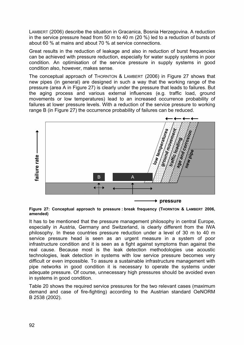
92

LAMBERT (2006) describe the situation in Gracanica, Bosnia Herzegovina. A reduction in the service pressure head from 50 m to 40 m (20 %) led to a reduction of bursts of about 60 % at mains and about 70 % at service connections. Great results in the reduction of leakage and also in reduction of burst frequencies can be achieved with pressure reduction, especially for water supply systems in poor condition. An optimisation of the service pressure in supply systems in good condition also, however, makes sense. The conceptual approach of THORNTON & LAMBERT (2006) in Figure 27 shows that new pipes (in general) are designed in such a way that the working range of the pressure (area A in Figure 27) is clearly under the pressure that leads to failures. But the aging process and various external influences (e.g. traffic load, ground movements or low temperatures) lead to an increased occurrence probability of failures at lower pressure levels. With a reduction of the service pressure to working range B (in Figure 27) the occurrence probability of failures can be reduced.

Figure 27: Conceptual approach to pressure : break frequency (THORNTON & LAMBERT 2006, amended)

It has to be mentioned that the pressure management philosophy in central Europe, especially in Austria, Germany and Switzerland, is clearly different from the IWA philosophy. In these countries pressure reduction under a level of 30 m to 40 m service pressure head is seen as an urgent measure in a system of poor infrastructure condition and it is seen as a fight against symptoms than against the real cause. Because most is the leak detection methodologies use acoustic technologies, leak detection in systems with low service pressure becomes very difficult or even impossible. To assure a sustainable infrastructure management with pipe networks in good condition it is necessary to operate the systems under adequate pressure. Of course, unnecessary high pressures should be avoided even in systems in good condition. Table 20 shows the required service pressures for the two relevant cases (maximum demand and case of fire-fighting) according to the Austrian standard OeNORM B 2538 (2002).

B A

pressure

failu

re ra

te

93

Table 20: Minimum service pressure in distribution mains according to OeNORM B 2538 (2002)

number of floors

required service pressure in bar required service pressure head in m

case 1: maximum demand

case 2: fire-fighting

case 1: maximum demand

case 2: fire-fighting

up to 3 3.0 1.7 30 17

4 3.6 2.2 36 22

5 4.2 2.7 42 27

6 4.8 3.2 48 32

4.7. Infrastructure Management Infrastructure management includes a very broad field of duties. One aspect is the configuration of the supply system and the technical equipment in use. The central tasks of infrastructure management are the duties of maintaining various objects (storage tanks, pumping stations etc.) and of the supply network, including all kinds of fittings, hydrants and flow meters. Figure 28 gives an overview of the maintenance duties. Rehabilitation planning is especially important for water loss management (including strategic rehabilitation planning, analyses of failure rates, long and mid term planning, etc.). Another topic is the customer meter management (type and age of customer meters, automatic meter reading or meter reading by personnel of water supply utility over larger periods of the year, key date problem) which has a great influence on the accuracy of water balance input-data. In general, infrastructure management activities are long term measures.

Figure 28: Maintenance duties (OVGW W 100, 2007)

When translating Figure 28 from German into English a problem occurred with the terms “rehabilitation” and “renovation”. In English the term “renovation” also stands for renewal, rehabilitation, refurbishment and sanitation. In our case “renovation” stands for the German word “Sanierung”. ALEGRE et al. (2006) uses the term “renovation” with the same meaning. The renovation of mains can be done with epoxy resine, cement mortar or other materials.

maintenance

inspectionservice reconditioning

rehabilitation repair

cleaning renovation renewal

failure

94

5. The process benchmarking system for managing physical water losses

5.1. General remarks After the introductory chapters about performance indicators, benchmarking, and water loss management, chapter 5 and chapter 6 represent the core of this PhD thesis: the process benchmarking system for the management of physical water losses. The challenge is to apply the methodology of process benchmarking to the topic of physical water loss management. To reach this aim the first step is the definition of a clear process structure (Figure 29). The process benchmarking system was created on the basis of the process structure described in chapter 5.2. This system consists of a part system for data collection (basis data, variables, context information) and a part system for data evaluation (performance indicators, quality matrix).

Figure 29: Methodology in developing the process benchmarking system

A big advantage for the successful development of this process benchmarking system was the possibility of a field test of the system developed within the 2007 OVGW process benchmarking project. Eleven water supply utilities in Austria with different supply structures and very different strategies in water loss management participated in this first project. The methodology chosen, with an extensive and hierarchical system of performance indicators, is a worldwide innovation. Selected results of this case study were first published by KOELBL et al. (2008a). Chapter 6 includes a detailed summary of the 2007 OVGW process benchmarking on physical water loss management. Many important methodological findings were realised during the field test. The process benchmarking system described in this work varies in some points from the 2007/08 OVGW system because the experiences of the field test were implemented to the process benchmarking system for the management of physical water losses. Some very important improvements made after the field test are discussed in the following chapters which describe the process structure and the process benchmarking system.

definition of process structure

development of benchmarking system

implementation of experiences of field test

field test of system

95

Before starting with the description of the process benchmarking system the criteria for the process benchmarking system described in chapter 1.2 should be summarised:

• Clear process structure: The process structure has to be easy to understand and all parts of the process (sub processes, supporting processes) have to be well defined.

• Hierarchical process structure: The process structure has to be hierarchical, so that both the overall performance and the performance in single parts of the process can be assessed.

• Practical applicability: The system of process benchmarking has to be in step with actual practice and, therefore, it has to be developed closely with water supply utility experts.

• For all structures: The system has to be applicable for all structures and all sizes of water supply utilities.

• Simple data gathering: The allocation of costs should be simple. The query of context-information should be done with selective lists to keep the effort as low as possible.

• Transparency: The system has to be a transparent one: “black-box” solutions have to be avoided.

• Data quality: The accuracy and reliability of variables has to be considered.

• Structural parameters: The system should consider different frame conditions of water supply systems to allow a performance comparison in “comparable” groups (clusters).

• Voluntary and anonymous system: The system should be used for voluntary benchmarking and should allow anonymous evaluations.

• Field test: The system has to stand a field test in the Austrian water supply sector.

5.2. Process mapping of physical water loss management As mentioned before, the process structure has to be easy to understand and all the parts of the process (sub processes, supporting processes) have to be well defined. Thus, first of all definitions of which duties a water supply utility has in the whole value chain have to be considered in the process of physical water loss management. Figure 30 gives an overview about all the different tasks that influence physical water loss management. It becomes clear that the process of physical water loss management is a highly integrative process which is influenced by many single tasks of almost all the operating duties of a water supply utility. Therefore it is not possible to handle this process as a part of a holistic process benchmarking system which covers the whole value chain. It is especially important to define the borders a process starts and ends for the definition of a selective process. The characteristics of this process and all the input and output factors of all the sub processes also need to be defined. It has to be specified what can be measured and how costs can be allocated. At the end of the

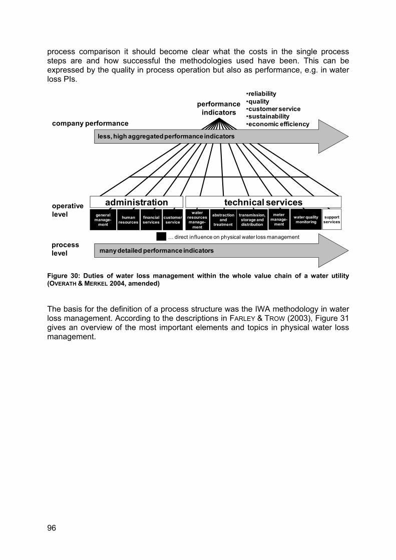
96

process comparison it should become clear what the costs in the single process steps are and how successful the methodologies used have been. This can be expressed by the quality in process operation but also as performance, e.g. in water loss PIs.

Figure 30: Duties of water loss management within the whole value chain of a water utility (OVERATH & MERKEL 2004, amended)

The basis for the definition of a process structure was the IWA methodology in water loss management. According to the descriptions in FARLEY & TROW (2003), Figure 31 gives an overview of the most important elements and topics in physical water loss management.

administration technical servicesgeneral

manage-ment

human resources

financial services

customer service

water resources manage-

ment

abstraction and

treatment

transmission, storage and distribution

meter manage-

ment

water quality monitoring

support services

less, high aggregated performance indicators

many detailed performance indicators

company performance

operative level

process level

performanceindicators

•reliability•quality•customer service•sustainability•economic efficiency

… direct influence on physical water loss management

97

Figure 31: Elements of physical water loss management (on basis of FARLEY & TROW 2003, amended)

Ann

ual L

osse

s •

accu

racy

of w

ater

bal

ance

dat

a •

PIs

(%, m

³/km

·h, l

/con

n·d,

ILI)

• ec

onom

ic le

vel o

f lea

kage

(ELL

) •

polic

ies

(cus

tom

er m

eter

ing,

tarif

f st

ruct

ure,

unb

illed

con

sum

ptio

n)

Pres

sure

Man

agem

ent

Act

ive

Leak

age

Con

trol

(A

LC)

Spee

d an

d Q

ualit

y of

R

epai

r

Infr

astr

uctu

re M

anag

emen

t re

habi

litat

ion

of m

ains

and

ser

vice

con

nect

ions

: •

aver

age

age

of m

ains

(pip

e gr

oups

) •

aver

age

age

of s

ervi

ce c

onne

ctio

ns (p

ipe

grou

ps)

• fa

ilure

sta

tistic

s (e

.g. b

urst

rate

s)

• cu

rren

t reh

abili

tatio

n ra

tes

(last

10

year

s)

mai

nten

ance

and

reha

bilit

atio

n of

oth

er in

frast

ruct

ural

faci

litie

s:

• pu

mps

, val

ves

and

flow

met

ers

• st

orag

e ta

nks

netw

ork

mod

ellin

g:

• an

alys

e th

e pr

esen

t and

futu

re c

apac

ity o

f the

wat

er d

istri

butio

n sy

stem

•

iden

tify

curre

nt a

nd fu

ture

hyd

raul

ic w

eak

poin

ts a

nd s

tagn

atio

n zo

nes

awar

enes

s tim

e:

• tim

e to

bec

ome

awar

e th

at b

urst

ex

ists

•

depe

ndin

g on

tech

nolo

gy

o

less

than

24

h o

3-

4 da

ys o

r eve

n m

uch

long

er

loca

tion

time:

•

num

ber o

f sta

ff av

aila

ble

• te

chno

logy

•

capa

bilit

ies

and

effic

ienc

y of

leak

lo

catio

n st

aff

repa

ir tim

e:

• so

me

hour

s up

to m

onth

s re

pair

cost

s:

• av

erag

e co

sts

of b

urst

repa

ir

effe

cts

(ben

efits

): •

redu

ctio

n of

leak

age

• re

duct

ion

of p

ress

ure

rela

ted

cons

umpt

ion

(e.g

. sho

wer

) •

redu

ctio

n of

freq

uenc

y of

bur

sts

• pr

otec

tion

of lo

ng-te

rm li

fe o

f ass

ets

(e.g

. joi

nts,

fitti

ngs)

pe

rman

ent o

r tem

pora

ry (d

urin

g ni

ght h

ours

) pre

ssur

e re

duct

ion

pres

sure

mon

itorin

g (p

erm

anen

t and

tem

pora

ry d

ata

logg

ers)

flow

met

erin

g (le

akag

e m

onito

ring)

: •

type

s of

met

ers

(acc

urac

ies)

o

m

echa

nica

l o

el

ectro

mag

netic

o

ul

traso

nic

o

poin

t vel

ocity

met

ers

(inse

rtion

met

ers)

•

data

logg

ers,

tele

met

ry

• ni

ght f

low

mon

itorin

g m

ulti-

para

met

er m

easu

rem

ents

•

flow

, pre

ssur

e, n

oise

D

MA

s (d

istri

ct m

eter

are

as):

• 10

.000

-50.

000

prop

ertie

s o

flo

w m

easu

rem

ent

• up

to 3

.000

pro

perti

es

o

perm

anen

t flo

w m

onito

ring

• 50

0-1.

000

conn

ectio

ns

o

tem

pora

ry z

ones

whi

le A

LC

leak

det

ectio

n:

• st

ep-te

stin

g •

nois

e lo

ggin

g •

soun

ding

sur

vey

o

soun

ding

stic

k (b

asic

, el

ectro

nic)

o

gr

ound

mic

roph

one

o

leak

noi

se c

orre

lato

r •

gas

inje

ctio

n (S

F 6, i

ndus

trial

hy

drog

en, H

e)

• ty

pes

of c

ontra

ct

o

paym

ent b

y re

sult

or ti

me

98

The process structure developed for the 2007 OVGW process benchmarking foresees a subdivision of the overall process into four sub processes and two supporting processes (Figure 32). The four sub processes are:

• leakage monitoring,

• leak detection,

• leak repair and

• analyses & planning. The two supporting processes are

• infrastructure management and the

• qualification of staff.

Figure 32: Original 2007 OVGW process structure for managing physical water losses

It can be seen that there is no sub process of pressure management. Pressure management is “only” considered as a part within the supporting process of infrastructure management. The reason for this is that pressure management in Austria is not as big a topic as it is internationally. In general, the Austrian water supply networks are operated with average service pressures between 3 and 5 bar. Due to aspects of customer service a reduction of service pressure under 3 bars has to be avoided. From the Austrian point of view, pressure reduction should only be a short-term measure and the aim of each utility should be to make adequate – but not unnecessary high - service pressures available. The precondition is an infrastructure in good condition. Concerning assessment of efficiency and process quality, the idea was to calculate costs and working times for all of the sub processes and to ask for a lot of context information regarding sub processes and supporting processes for the assessment of

 

Leakage Monitoring

Leak Detection

Leak Repair

Analyses & Planning

1) process quality ofeach sub-process

2) results qualityof overall process

- PIs- background

informationQ U A L I T Y

Infrastructure Management / (Physical) Asset Management- network instrumentation - inspection & maintenance - pressure management- rehabilitation - customer meter management

supporting processes

- system input- night minimum monitoring- DMA`s- …- awareness time

- step testing- sounding stick- leak noise correlator- …- location time

- repair technology- failure documentation- condition of pipes- … - repair time

Qualification of staff / (Intangible) Asset Management

- overall analyses- water loss PIs- optimisations in WLM- …

Costs TimeEFFICIENCY

99

the quality in process operation. No costs and working times are analysed for the supporting processes because the allocation of cost would be too difficult and the result would also be distorted. In fact, these supporting processes are often much more cost intensive (e.g. the process of rehabilitation) than the process of physical water loss management itself. This problem was also realised with the leak repair sub process. A participating utility mentioned that the costs for the sub process leak repair in the company are nearly ten times higher than the costs for the rest of the process of physical water loss management. Therefore no costs for this sub process are considered in the overall process. However, for questions like the long-term economic level of leakage the costs for leak repair and also costs of other supporting processes like rehabilitation have to be taken into account (e.g. FARLEY & TROW 2003). Therefore for this sub process, as well as for some infrastructural management tasks, annual costs (e.g. depreciation costs for investments) are considered as context information. This information is available for additional analyses but these costs are not part of the overall performance in physical water loss management. In fact, the sub process leak repair should better be defined as a supporting process and, therefore, the process structure changes to a subdivision of three sub processes (Figure 33).

Figure 33: Adapted process structure for managing physical water losses

5.2.1. Sub processes of physical water loss management

5.2.1.1. Leakage Monitoring The aim of the leakage monitoring sub process is to become aware of a failure caused increasing of the system input and / or recognising the exceeding of quantitative thresholds (flow, pressure, noise) and receiving the first information “where” the leakage is located (e.g. which district).

100

The following technologies are part of this sub process:

• flow measurements of system input (e.g. at wells, springs or storage tanks)

• zonal flow measurements (flow meters of DMAs)

• pressure measurements

• noise loggers (permanently installed in the network)

• combined (mulitparameter) measurements of flow, pressure and noise Other aspects of this sub process are process control systems (SCADA) and their functionality for the purposes of water loss management and software tools for leakage monitoring. Figure 34 shows the input and output criteria and quality criteria for the input and output of this sub process.

Figure 34: Leakage monitoring sub process

5.2.1.2. Leak detection The aim of the sub process leak detection is the localisation of failures (leakage) in the supply network. The sub process starts due to advance information from the sub process leakage monitoring (caused based leak detection strategy) or is undertaken in routine leak detection campaigns on a rotational basis (e.g. once a year or larger intervals). The sub process results in the localisation of failures (leakages) and, if possible, information about the condition of pipes should also be generated (e.g. number of failures or the volume of water lost on a pipe section). This information can support the decision to repair or rehabilitate the affected pipe section (Figure 35). Various leak detection methodologies belong to this sub process:

• step testing

• sounding surveys o sounding stick o ground microphone

OUTPUT• recognition of a failure caused

increasing of system input• exceeding of quantitative thresholds

(flow, pressure, noise)• first information about leak location

INPUT• system-input metering• district meter areas (DMAs)• SCADA system• leakage monitoring software• pressure and noise loggers• combined measurements (flow,

pressure, noise)• personnel

leakagemonitoring

QUALITY CRITERIA• awareness time• accuracy of system and DMA input-data• significance of night minimum consumption• potential in narrowing down the area of leak

location on basis of monitoring data

QUALITY CRITERIA• type of meter, date of calibration• size of DMAs• functions of SCADA system (data transmission

interval, connected objects)• automated quantitative thresholds• evaluation night minimum consumption• density of flow, noise and pressure

measurements• qualification of staff

OUTPUT• recognition of a failure caused

increasing of system input• exceeding of quantitative thresholds

(flow, pressure, noise)• first information about leak location

INPUT• system-input metering• district meter areas (DMAs)• SCADA system• leakage monitoring software• pressure and noise loggers• combined measurements (flow,

pressure, noise)• personnel

leakagemonitoring

QUALITY CRITERIA• awareness time• accuracy of system and DMA input-data• significance of night minimum consumption• potential in narrowing down the area of leak

location on basis of monitoring data

QUALITY CRITERIA• type of meter, date of calibration• size of DMAs• functions of SCADA system (data transmission

interval, connected objects)• automated quantitative thresholds• evaluation night minimum consumption• density of flow, noise and pressure

measurements• qualification of staff

101

o leak noise correlator o noise loggers (temporarily installed)

• gas injection Often smaller water utilities do not have personnel resources and adequate leak detection equipment. Therefore this sub process, or parts of it, is often outsourced to external specialists.

Figure 35: Leak detection sub process

5.2.1.3. Analyses & Planning The aim of the analyses and planning sub process is to analyse the whole process of physical water loss management regarding efficiency and effectiveness at regular intervals, and to also define measures for improvement in infrastructure (e.g., metering systems, DMAs) as well as in process operation (e.g., staff education programmes, optimisation of operating instructions) (Figure 36). But the calculation of performance indicators, failure statistics and analyses and preparation of data for supporting processes (e.g. rehabilitation planning) are also part of this sub process.

OUTPUT• localisation of failures• information about condition of pipes• decision support:

- repair or rehabilitation

INPUT• leak detection equipment• strategy

- cause related leak detection- routine survey on a rotational

basis (mains and/or service connections)

• personnel of water utility• external specialists

leak detection

QUALITY CRITERIA• location time• accuracy of leak detection• hit rate (all leaks founds?)• documentation of leak detection (where,

when, what methodology)

QUALITY CRITERIA• available equipment

- temporary noise loggers- listening stick, ground microphone- leak noise correlator- tracer gas etc.

• advance information of leakage monitoring• qualification of staff• type of contract of external specialists

(e.g. performance based)

OUTPUT• localisation of failures• information about condition of pipes• decision support:

- repair or rehabilitation

INPUT• leak detection equipment• strategy

- cause related leak detection- routine survey on a rotational

basis (mains and/or service connections)

• personnel of water utility• external specialists

leak detection

QUALITY CRITERIA• location time• accuracy of leak detection• hit rate (all leaks founds?)• documentation of leak detection (where,

when, what methodology)

QUALITY CRITERIA• available equipment

- temporary noise loggers- listening stick, ground microphone- leak noise correlator- tracer gas etc.

• advance information of leakage monitoring• qualification of staff• type of contract of external specialists

(e.g. performance based)

102

Figure 36: Analyses & planning sub process

5.2.2. Supporting Processes Beside the three sub processes, the two supporting processes of infrastructure management (e.g. repair, inspection and maintenance, rehabilitation, pressure management or customer meter management) and qualification of staff are also very important for the process of physical water loss management.

5.2.2.1. Infrastructure Management (Physical Asset Management) Infrastructure management covers various tasks which directly or indirectly influence the amount of water losses. Beside a water supply utility’s technical equipment, the rehabilitation management (including analyses of failure statistics based on pipe groups), the management of maintenance (fittings, pumps, flow meters, valves etc.) and also the customer meter management (average age of customer meters, methodology of meter reading etc.), hydraulic modelling of the supply system and the repair of failures are part of this supporting process. In general, infrastructure management covers long-term measures and many of them can not be influenced over short time periods.

5.2.2.1.1. Leak Repair Because of its importance for the overall process of physical water loss management and the former status as a sub process, the supporting process of leak repair is briefly described. Faults are repaired, the operating function of the affected pipe sections is re-established and water losses should be reduced within the supporting process of leak repair (Figure 37). The supporting process of leak repair starts after the localisation of failures and contains all the working steps of the leak repair. Another important aspect of leak repair is the failure documentation which gives:

• information about the condition of pipes

• a decision support for rehabilitation planning (repair or replace)

• and is the basis for the adaptation of the inspection and maintenance strategy

OUTPUT• performance indicators • failure statistics • effectiveness and efficiency of whole

process• derivation of measures (system

adjustments)• database for maintenance and

rehabilitation planning

INPUT• data of leakage monitoring and leak

detection• failure documentation• costs for sub processes leakage

monitoring and leak detection• costs for leak repair• personnel

analyses & planning

QUALITY CRITERIA• type of used performance indicators (e.g. ILI,

pipe-group based failure rates)• period under consideration (annual, monthly)• appropriation of data for other processes

QUALITY CRITERIA• data accuracy of system and DMA input

measurements• quality of failure documentation• accuracy of costs (e.g. documentation of working

time)• qualification of staff

OUTPUT• performance indicators • failure statistics • effectiveness and efficiency of whole

process• derivation of measures (system

adjustments)• database for maintenance and

rehabilitation planning

INPUT• data of leakage monitoring and leak

detection• failure documentation• costs for sub processes leakage

monitoring and leak detection• costs for leak repair• personnel

analyses & planning

QUALITY CRITERIA• type of used performance indicators (e.g. ILI,

pipe-group based failure rates)• period under consideration (annual, monthly)• appropriation of data for other processes

QUALITY CRITERIA• data accuracy of system and DMA input

measurements• quality of failure documentation• accuracy of costs (e.g. documentation of working

time)• qualification of staff

103

Figure 37: Leak repair supporting process

5.2.2.2. Qualification of staff (Intangible Asset Management) A well qualified staff is important for almost all the duties of water supply utilities. But for the process of physical water loss management these intangible assets are of especially great relevance. High technological leak detection equipment requires know-how and experience. Because this process covers so many aspects of many different fields of duties it is necessary to train the staff to think in “terms of water loss management”, meaning keeping their eyes open and building up integrative understanding of the complexity of water supply systems, especially of pipe networks.

5.3. Data collection system The data collection system developed consists of five parts (Table 21):

• contact details

• basis data

• water supply system data

• water balance data

• process specific data There are three different types of collected data:

• variables

• supporting information and

• context information Variables are data used for the calculation of performance indicators whereas context information is generally used for the evaluation of the process quality within the quality matrix and as background information for data interpretation. Some variables are aggregated data which are calculated of the supporting data gathering tables, e.g. within the water balance or basis data. All the elements of the data collection system (except supporting data) are indicated by a code. If the definitions of data elements are the same as those in the IWA-PI

OUTPUT• cleared fault• restoration of operativeness• failure documentation• information about condition of pipes • decision support:

- rehabilitation (yes/no)• adaptation of inspection and

maintenance strategy

INPUT• information about leak location• material (pipe clamp or pipe section)• personnel of water utility• external service (e.g. digging)

leak repair

QUALITY CRITERIA• repair time• reduction of leakage• quality of repair• failure documentation (documentation criteria,

kind and cause of damage)

QUALITY CRITERIA• product quality of repair material• qualification of staff

OUTPUT• cleared fault• restoration of operativeness• failure documentation• information about condition of pipes • decision support:

- rehabilitation (yes/no)• adaptation of inspection and

maintenance strategy

INPUT• information about leak location• material (pipe clamp or pipe section)• personnel of water utility• external service (e.g. digging)

leak repair

QUALITY CRITERIA• repair time• reduction of leakage• quality of repair• failure documentation (documentation criteria,

kind and cause of damage)

QUALITY CRITERIA• product quality of repair material• qualification of staff

104

system (ALEGRE et al. 2006) the IWA-codes are also described within squared brackets in the tables of the appendix, where the whole data collection system is described in detail.

Table 21: Structure of data collection system

data element variables supporting information

context information total

contact data - - 20 20

basis data - ≥ 3 7 ≥10

water supply system data 21 - - 21

water balance data 22 ≥ 53 2 ≥ 77

process specific data 85 - 168 253

total 128 ≥ 56 197 ≥ 381

5.3.1. Data accuracy Knowledge about data accuracy is essential for all types of performance comparisons. Therefore this process benchmarking system also includes data accuracy and reliability. There are two different kinds of indication of data accuracy and reliability:

• direct indication of the error margin as percentages of the input value

• indirect indication using the indicators A to D o A: very reliable data, error margin ± < 5 % o B: reliable data, error margin ± 5 to 25 % o C: unreliable data, error margin ± 25 to 100 % o D: very unreliable data, error margin ± > 100 %

Direct indications of error margins are used, for example, for water balance data and for some water supply system data like distribution mains length or the average service connection length.

5.3.2. Contact details Beside the company’s name, address and fax number the contact data (first and second name, title, sex, telephone number, email address) of the responsible person for the process benchmarking within the company and of a representative are also collected (Table 49 in appendix).

5.3.3. Basis data Basis data include background information about a given water supply utility and supporting information about hourly rates of employees. This is used for the calculation of personnel costs for each sub process by multiplying the working time for a sub process of each employee or each employee group with the hourly rates (Table 50 and Table 51 in appendix).

105

5.3.4. Water supply system data Water supply system data include variables about the structure (mains length, number of service connections, service pressure) and the instrumentation (number of DMAs, metering systems, pressure and noise loggers and pressure reduction valves) of the water supply system (Table 52 in appendix). The data accuracy is specified with the indirect indication A to D for all water supply system data except for the “average service pressure head”, “distribution mains length” and “average service connection length” variables which are indicated directly (with possible error margins in percentages).

5.3.5. Water balance data All the water balance data are variables or supporting data for the calculation of aggregated variables (Table 53 to Table 63 in appendix) except for two single data of context information. The water balance data collection system is designed along a flow chart from water abstraction to water treatment to water consumption and water losses like those described in LAMBERT & HIRNER (2000). It is possible to give detailed answers for each single relevant point of the supply system for almost all water balance data (e.g. for abstracted water it is possible to describe each single well and each natural spring) which are generated to summarised variables. The total amount of abstracted water is generated by summing up all single data and the data accuracy for the total amount of abstracted water is calculated by weighted data (according to abstracted volumes) from single data sets. The data accuracy for all water balance data is indicated directly by error margins in percentages. The assessment period for water balance data is one year.

5.3.6. Process specific data Process specific data include variables and context information for the three sub processes of leakage monitoring, leak detection and analyses and planning and for the supporting processes of infrastructure management and qualification of staff. A data collection matrix for cost and working time data for each of the sub processes is used to evaluate the (sub-) process efficiencies (Table 22). Three years of summarised data are collected for this purpose, to avoid pure comparability due to annual variations in process operation. The working hours are given for each single employee or each group of employees (e.g., engineers, plumbers). Together with basis data about the hourly rate of Table 51 (in appendix), the personal costs of the utility’s internal personal is calculated. Other running costs and material costs are declared in an extra field. If it is not possible to gather information about the working hours in an alternative field the summarised personal costs can be given. However, then a comparison of working hours is not possible. Beside the internal costs of a utility, outsourcing costs also have to be considered. Therefore costs of outsourcing in-house and external outsourcing are collected. If it is possible, working hours should be given but personal costs and material costs should be differentiated for these two types of costs.

106

The sum of these single cost types (internal, outsourcing in-house, outsourcing externally) gives the total running costs for a sub process. The working times are also summarised for the sub process. Beside the data itself, the reliability and accuracy of the data also needs to be specified.

Table 22: Data collection matrix for running costs and working time of sub processes

0,00

0,00

relia

bilit

y an

d ac

cura

cy o

f the

se d

ata

A

2.50

0,00

tota

l wor

king

tim

e of

sub

-pro

cess

[hh:

mm

]67

0:00

tota

l run

ning

cos

ts o

f sub

-pro

cess

[E

uro]

35.0

00,0

0

mat

eria

l co

sts:

sum

per

sona

l cos

ts u

tility

in

tern

28

.500

,00

othe

r run

ning

cos

ts a

nd m

ater

ial c

osts

util

ity in

tern

[E

uro]

mat

eria

l co

sts:

0,00

pers

onal

co

sts:

4.00

0,00

pers

onal

co

sts:

wor

king

tim

e:10

0:00

wor

king

tim

e:00

:00

sum

wor

king

tim

e ut

ility

inte

rn

570:

00

cost

s fo

r out

sour

cing

in

-hou

se(a

ppor

tionm

ent o

f per

sona

l an

d m

ater

ial c

osts

)

cost

s fo

r out

sour

cing

ex

tern

(per

sona

l and

mat

eria

l co

sts)

engi

neer

150:

00

4.00

0,00

0,00

tech

nici

an42

0:00

runn

ing

cost

s an

d w

orki

ng ti

me

of s

ub p

roce

ss

sum

of l

ast 3

yea

rs

(e.g

. 200

4, 2

005

und

2006

)

nam

e or

gro

up o

fem

ploy

ees

wor

king

tim

e[h

h:m

m]

e.g.

: 18:

35

pers

onal

cos

tsut

ility

inte

rn

(alte

rnat

ive,

if w

orki

ng-ti

me

base

d ca

lcul

atio

n of

pe

rson

al c

osts

is n

ot

poss

ible

)

107

5.3.6.1. Data of sub process leakage monitoring According to the data collection matrix described in Table 22, the variables for the sub process leakage monitoring are listed in Table 64 (in appendix). In addition to these variables, many data for background information and for quality assessment are collected (Table 65 in appendix). Investment costs for leakage monitoring equipment (e.g. flow meters, SCADA system) are not considered for efficiency evaluation in the 2007 OVGW process benchmarking system. The reason is that almost all the participants in the benchmarking working group were of the opinion that the definition of these costs is not clear enough because almost all of the leakage monitoring equipment is also used for other purposes like process control. Further, data gathering can be difficult because these systems were often installed together with other measures. However, experiences within the field test showed that there is a need to consider investment costs of monitoring systems for reasons of comparability. Therefore the two variables v114 and v115 in Table 64 (in appendix) are used to calculate depreciation costs for an assumed depreciation period of 10 years, which are added to the total costs of sub process leakage monitoring (v101). Another aspect which is not considered in the 2007 OVGW process benchmarking system is the methodology of multiparameter measurements described in chapter 4.5.2. Therefore an additional question as context information was implemented (ci107 in Table 65, in appendix).

5.3.6.2. Data of sub process leak detection Data gathering for running costs and working hours also follows the scheme described in Table 22. The variables for costs and working time are described in Table 66 (in appendix). Table 67 (in appendix) contains information about the current leak detection equipment and the investment cost for this equipment. On the basis of the original investment costs, depreciation costs for an assumed depreciation period of 10 years are calculated, which are added to the total costs for these sub process. Table 68 and Table 69 (in appendix) give an overview of the variables for assessment of leak detection measures and detected failures in the assessment period. Possible answers to context information data (Table 70 in appendix) with code ci201 to ci205 are described in detail in chapter 5.5.

5.3.6.3. Data of sub process analyses and planning Data of working hours and sub process costs are collected as for the other sub processes (Table 71 in appendix). There are no further cost data in this sub process except for some context information for process quality assessment, like questions about time intervals in which various analyses are operated or about which performance indicators are calculated for internal purposes or for publication, e.g. in annual reports (Table 72 and Table 73 in appendix).

5.3.6.4. Data of supporting process infrastructure management As mentioned before, no economic performance indicators are calculated for supporting processes but various kinds of context information is considered in the quality matrix, and a quality index for the supporting process is calculated.

108

Beside context information about network inspection, hydraulic modelling, pressure management, rehabilitation and customer meter management (Table 74 in appendix) activities in leak repair are also considered within this supporting process.

5.3.6.4.1. Data of supporting process leak repair For the leak repair supporting process, which is part of the infrastructure management supporting process, the following data are gathered (Table 75 to Table 79 in appendix):

• variables about number of repairs and about repair costs

• context information about repair time and information for planning

• context information about failure documentation

• context information about type of failures and

• context information about cause of failures.

5.3.6.5. Data of supporting process qualification of staff The last part of process specific data is some context information about the water supply utilities’ employees’ qualifications (Table 80 in appendix).

5.4. Process performance indicators Chapter 5.3 described the subsystem for data collection (variables, context information). As with the subsystem for data collection, the subsystem for data evaluation (performance indicators, quality matrix) is also based on the process structure. Figure 38 gives an overview of the number of variables, context information and the calculated performance indicators.

Figure 38: Process performance indicator system

The whole system of performance indicators for the process of physical water loss management consists of 66 PIs and 7 quality indices. Figure 39 shows the structure of performance indicators for the process of physical water loss management and gives an overview about the performance indicators calculated for the single sub- and supporting processes and for the main process (overall process).

water loss PIs     6main process PIs              10sub process PIs                 41supporting process PIs      9total                                    66

197context information

128 variables

7 quality indices

+ quality matrix

data collection evaluation

109

Figure 39: Structure of performance indicators

6 water loss PIs

10 main process PIs &

1 quality index

41sub process

PIs&

3 quality indices

sub processleakage

monitoring10 PIs &

1 quality index

sub processleak detection

21 PIs &1 quality index

sub processanalyses &

planning10 PIs &

1 quality index

supporting processes3 qualityindices

supportingprocess

leak repair9 sub-PIs

supportingprocesses

3 qualityindices

&9 sub-PIs

• water loss ratio• real losses per connection per day• real losses per connection per day per meter service pressure head• real losses per km per hour• ILI• non-revenue water

• total process costs per km mains• total process costs per 100 service conn.• utility internal costs per km mains• utility internal costs per 100 service conn.• outsourcing in-house costs per km mains• outsourcing in-house costs per 100 s. conn.

• outsourcing extern costs per km mains• outsourcing extern costs per 100 s. conn.• total working time per km mains• total working time per 100 service conn.

• quality index main process

• sub-process costs per km mains• sub-process costs per 100 service conn.• utility internal costs per km mains• utility internal costs per 100 service conn.• outsourcing in-house costs per km mains• outsourcing in-house costs per 100 s. conn.• outsourcing extern costs per km mains

•outsourcing extern costs per 100 s. conn.• working time per km mains• working time per 100 service conn.

• quality index leakage monitoring

• sub-process costs per km mains• sub-process costs per 100 service conn.• utility internal costs per km mains• utility internal costs per 100 service conn.• outsourcing in-house costs per km mains• outsourcing in-house costs per 100 s. conn.• outsourcing extern costs per km mains• outsourcing extern costs per 100 s. conn.• working time per km mains• working time per 100 service conn.• proportion of transportation mains annually

inspected by leak detection methodologies• proportion of distribution mains annually

inspected by leak detection methodologies• proportion of service connections annually

inspected by leak detection methodologies

• cause based leak detection:• localised leaks at transmission mains• localised leaks at distribution mains• localised leaks at service connections• portion of costs for cause based leak

detection

routine survey:• localised leaks at transmission mains• localised leaks at distribution mains• localised leaks at service connections• portion of costs for routine surveys

• quality index leak detection

• sub-process costs per km mains• sub-process costs per 100 service conn.• utility internal costs per km mains• utility internal costs per 100 service conn.• outsourcing in-house costs per km mains• outsourcing in-house costs per 100 s. conn.• outsourcing extern costs per km mains• outsourcing extern costs per 100 s. conn.

• working time per km mains• working time per 100 service conn.

• quality index analyses & planning

• quality index infrastructure management• quality index leak repair• quality index qualification of staff

• average repair costs of pipe failures / fitting failures at transmission mains• average repair costs of pipe failures / fitting failures at distribution mains• average repair costs of pipe failures / fitting failures at service connections• failure rate transmission mains• failure rate distribution mains• failure rate service connections

110

For both the main process and the sub processes, the costs and also the working time are calculated. Outsourcing (in-house and external) of tasks is also considered, and separately visualised. Except water loss PIs, which are calculated for a single year, all performance indicators are average values for the assessment period of three years.

5.4.1. Water loss PIs Table 23 gives an overview of the water loss PIs (note: abbreviation “WL” stands for Water Loss), which are calculated for the whole water supply system. Because the accuracy is specified in percentages of possible error margins for all water flow data, the accuracy of water loss PIs is also expressed in percentages. The codes used in row “calculation” are the variable codes (see appendix). A detailed description of all water loss PIs is given in chapter 4.4.

Table 23: Water loss PIs

code performance indicator calculation unit accuracy WL01 Water loss ratio (wb20 * 100) / wb07 % ± in %

WL02 Real losses per (total) mains length Wb20 / (v004 * 8760) m³/km·h ± in %

WL03 [Op27]

Real losses per connection and day (wb20 * 1000) / (v005 * 8760) [l/conn·d] ± in %

WL04 Real losses per connection and day per metre service pressure

(wb20 * 1000) / (v005 * 8760 * v007)

l/conn·d·m ± in %

WL05 [Op29]

Infrastructure Leakage Index (ILI)

[CARL / UARL] definition see chapter 4.4.5 [-] ± in %

WL06 [Fi46] Non-revenue water (NRW) [(wb21 * 100) / wb07] [%] ± in %

[IWA Code], [IWA definition] and [IWA unit]…according to ALEGRE et al. (2006)

5.4.2. Main process PIs The ten economic main process PIs (M01-M10) are summarised values of the three sub processes of leakage monitoring, leak detection and analyses & planning, which are structured in the same way as the main process PIs (Table 24). The economic indicators (for the main process and for the sub processes) are structured into the 5 different topics:

• total process (or sub process) cost

• utility internal costs

• outsourcing in-house costs

• outsourcing extern costs

• working time and each of these PIs is expressed as:

• Euro per kilometre of distribution mains per year (€/km·a) and as

• Euro per service connection per year (€/conn·a). The data accuracy for economic indicators is expressed in categories A-D.

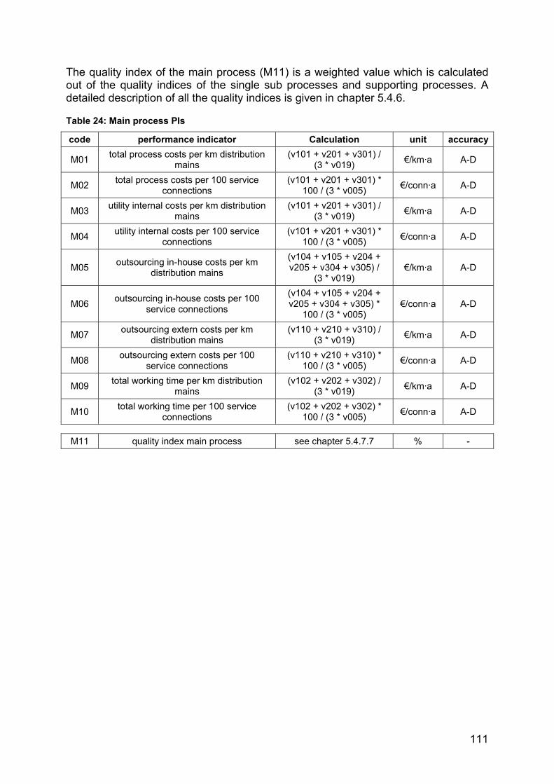
111

The quality index of the main process (M11) is a weighted value which is calculated out of the quality indices of the single sub processes and supporting processes. A detailed description of all the quality indices is given in chapter 5.4.6.

Table 24: Main process PIs

code performance indicator Calculation unit accuracy

M01 total process costs per km distribution mains

(v101 + v201 + v301) / (3 * v019) €/km·a A-D

M02 total process costs per 100 service connections

(v101 + v201 + v301) * 100 / (3 * v005) €/conn·a A-D

M03 utility internal costs per km distribution mains

(v101 + v201 + v301) / (3 * v019) €/km·a A-D

M04 utility internal costs per 100 service connections

(v101 + v201 + v301) * 100 / (3 * v005) €/conn·a A-D

M05 outsourcing in-house costs per km distribution mains

(v104 + v105 + v204 + v205 + v304 + v305) /

(3 * v019) €/km·a A-D

M06 outsourcing in-house costs per 100 service connections

(v104 + v105 + v204 + v205 + v304 + v305) *

100 / (3 * v005) €/conn·a A-D

M07 outsourcing extern costs per km distribution mains

(v110 + v210 + v310) / (3 * v019) €/km·a A-D

M08 outsourcing extern costs per 100 service connections

(v110 + v210 + v310) * 100 / (3 * v005) €/conn·a A-D

M09 total working time per km distribution mains

(v102 + v202 + v302) / (3 * v019) €/km·a A-D

M10 total working time per 100 service connections

(v102 + v202 + v302) * 100 / (3 * v005) €/conn·a A-D

M11 quality index main process see chapter 5.4.7.7 % -

112

5.4.3. PIs of leakage monitoring sub process The PIs of leakage monitoring sub process are in the same structure as the main PIs (Table 25).

Table 25: PIs of leakage monitoring sub process

code performance indicator Calculation unit accuracy

S101 sub process leakage monitoring costs per km distribution mains v101 / (3 * v019) €/km·a A-D

S102 sub process leakage monitoring costs per 100 service connections v101 * 100 / (3 * v005) €/conn·a A-D

S103 sub process leakage monitoring utility internal costs per km distribution mains (v104 + v105) / (3 * v019) €/km·a A-D

S104 sub process leakage monitoring utility internal costs per 100 service connections

(v104 + v105) * 100 / (3 * v005) €/conn·a A-D

S105 sub process leakage monitoring

outsourcing in-house costs per km distribution mains

v106 / (3 * v019) €/km·a A-D

S106 sub process leakage monitoring

outsourcing in-house costs per 100 service connections

v106 * 100 / (3 * v005) €/conn·a A-D

S107 sub process leakage monitoring outsourcing extern costs per km

distribution mains v110 / (3 * v019) €/km·a A-D

S108 sub process leakage monitoring

outsourcing extern costs per 100 service connections

v110 * 100 / (3 * v005) €/conn·a A-D

S109 sub process leakage monitoring working time per km distribution mains v102 / (3 * v019) €/km·a A-D

S110 sub process leakage monitoring working time per 100 service connections v102 * 100 / (3 * v005) €/conn·a A-D

S111 quality index leakage monitoring sub process see chapter 5.4.7.1 % -

5.4.4. PIs of leak detection sub process For the sub process of leak detection, beside the ten economic PIs and the quality index (Table 26), technical PIs about the leak detection activities (Table 27) and localised leaks at transmission, distribution mains and at service connections (Table 28) in the assessment period are also calculated.

113

Table 26: Economic PIs and quality index of leak detection sub process

code performance indicator Calculation unit accuracy

S201 sub process leak detection costs per km distribution mains v201 / (3 * v019) €/km·a A-D

S202 sub process leak detection costs per 100 service connections v201 * 100 / (3 * v005) €/conn·a A-D

S203 sub process leak detection utility internal costs per km distribution mains (v204 + v205) / (3 * v019) €/km·a A-D

S204 sub process leak detection utility internal costs per 100 service connections

(v204 + v205) * 100 / (3 * v005) €/conn·a A-D

S205 sub process leak detection outsourcing in-house costs per km distribution mains v206 / (3 * v019) €/km·a A-D

S206 sub process leak detection outsourcing in-house costs per 100 service connections v206 * 100 / (3 * v005) €/conn·a A-D

S207 sub process leak detection outsourcing extern costs per km distribution mains v210 / (3 * v019) €/km·a A-D

S208 sub process leak detection outsourcing extern costs per 100 service connections v210 * 100 / (3 * v005) €/conn·a A-D

S209 sub process leak detection working time per km distribution mains v202 / (3 * v019) €/km·a A-D

S210 sub process leak detection working time per 100 service connections v202 * 100 / (3 * v005) €/conn·a A-D

S211 quality index leak detection sub process see chapter 5.4.7.2 % - Table 27: Leak detection activities in assessment period

code performance indicator calculation unit accuracy

S212 proportion of transmission mains annually

inspected by leak detection methodologies

(v234a + v234b) * 100 / (3 * v018) % A-D

S213 proportion of distribution mains annually

inspected by leak detection methodologies

(v234c + v234d) * 100 / (3 * v019) % A-D

S214 proportion of service connections annually

inspected by leak detection methodologies

(v237 + v237a) * 100 / (3 * v005) % A-D

S215 portion of costs for routine surveys v235 * 100 / v201 % A-D

S216 portion of costs for cause based leak detection v236 * 100 / v201 % A-D

114

Table 28: Localised leaks in relation to the inspected pipe length rather number of inspected service connections

code performance indicator calculation Unit accuracy

S217 localised leaks at transmission mains by routine surveys v239 * 100 / (3 * v234a) No./100 km·a A-D

S218 localised leaks at transmission mains by cause based leak detection v240 * 100 / (3 * v234b) No./100 km·a A-D

S219 localised leaks at distribution mains by routine surveys v242 * 100 / (3 * v234c) No./100 km·a A-D

S220 localised leaks at distribution mains by cause based leak detection v243 * 100 / (3 * v234d) No./100 km·a A-D

S221 localised leaks at service connections by routine surveys v245 * 1000 / (3 * v237) No./1000

conn·a A-D

S222 localised leaks at service connections by cause based leak detection

v246 * 1000 / (3 * v237a)

No./1000 conn·a A-D

5.4.5. PIs of analyses & planning sub process Ten economic PIs and a quality index are calculated for this sub process (Table 29).

Table 29: PIs of analyses & planning sub process

code performance indicator definition/calculation unit accuracy

S301 sub process analyses & planning costs per km distribution mains v301 / (3 * v019) €/km·a A-D

S302 sub process analyses & planning costs per 100 service connections v301 * 100 / (3 * v005) €/conn·a A-D

S303 sub process analyses & planning utility internal costs per km distribution mains (v304 + v305) / (3 * v019) €/km·a A-D

S304 sub process analyses & planning utility internal costs per 100 service connections

(v304 + v305) * 100 / (3 * v005) €/conn·a A-D

S305 sub process analyses & planning

outsourcing in-house costs per km distribution mains

v306 / (3 * v019) €/km·a A-D

S306 sub process analyses & planning

outsourcing in-house costs per 100 service connections

v306 * 100 / (3 * v005) €/conn·a A-D

S307 sub process analyses & planning outsourcing extern costs per km

distribution mains v310 / (3 * v019) €/km·a A-D

S308 sub process analyses & planning

outsourcing extern costs per 100 service connections

v310 * 100 / (3 * v005) €/conn·a A-D

S309 sub process analyses & planning working time per km distribution mains v302 / (3 * v019) €/km·a A-D

S310 sub process analyses & planning working time per 100 service connections v302 * 100 / (3 * v005) €/conn·a A-D

S311 quality index analyses & planning sub process see chapter 5.4.7.3 % -

115

5.4.6. Sub-PIs of leak repair supporting process Six performance indicators about average repair costs and three indicators about average failure rates of the three year assessment period are calculated for the leak repair supporting process (Table 30).

Table 30: PIs of leak repair supporting process

code performance indicator definition/calculation Unit accuracy

R101 average repair costs of pipe failures at transmission mains v507 / v501 € A-D

R102 average repair costs of pipe failures at distribution mains v508 / v502 € A-D

R103 average repair costs of pipe failures at service connections v509 / v503 € A-D

R104 average repair costs of fitting failures at transmission mains v510 / v504 € A-D

R105 average repair costs of fitting failures at distribution mains v511 / v505 € A-D

R106 average repair costs of fitting failures at service connections v512 / v506 € A-D

R107 failure rate transmission mains v501 / (3 * v018) No./100 km·a A-D R108 failure rate distribution mains v502 * / (3 * v019) No./100 km·a A-D

R109 failure rate service connections v503 / (3 * v005) No./1000 conn·a A-D

5.4.7. Quality indices The aim of quality indices (QI) is to quantify the quality in process operation. Therefore many individual questions are asked for each sub and supporting process (see chapter 5.3.6 and chapter 5.5). Most of these questions allow five possible answers (from low to high performance). Beside quality indices for sub and supporting processes, a quality index for the main process (chapter 5.4.7.7) is also calculated. The systematic for the calculation of the quality indices for the leakage monitoring sub process is described in chapter 5.4.7.1.

5.4.7.1. QI of leakage monitoring sub process Table 31 shows the quality index for the sub process of leakage monitoring. The calculation of the quality indices is discussed in the following section on the basis of this example.

116

Table 31: Quality index of leakage monitoring sub process

A maximum of 4 points can be attained for each single criterion (column D). These points are weighted (column E), which leads to a maximum number of points for the whole sub or supporting process by multiplying the points of D with the weighting of E and summing up all these values. In the example of sub process leakage monitoring a maximal number of 296 points can be reached (column F). The quality index for this sub process (column H) is calculated by dividing the points reached (column G) by the maximum possible number of points (column F). Practices in system metering, functions of SCADA systems, practises in pressure and noise logging and the size of measuring zones are especially relevant criteria for the quality of sub process leakage monitoring. On the basis of these criteria it should be possible to determine how well the supply system can be monitored regarding leakage.

A B C D E F G H

sub or supporting

processCode Criteria

maximum points for

single criteria

weighting within sub or supporting

process

max. points of sub or

supporting process

reached points

quality index of sub or

supporting process

1.1 system input metering 4 5

1.2 district metered areas (DMA) 4 5

1.3 evaluation of night minimum consumption 4 5

1.4 SCADA system 4 2

1.4.1 functions of SCADA system 4 1

1.4.1.1 data transmission interval system input data 4 1

1.4.1.2 data transmission interval DMA input data 4 1

1.4.1.3 data transmission interval pressure data 4 1

1.4.1.4 data transmission interval reservoir level 4 1

1.4.1.5 data transmission interval pumping station data 4 1

1.4.2 automated evaluation of night minimum consumption 4 1

1.4.3 automated alarm when tresholds exceeded 4 1

1.5 pressure monitoring 4 51.6 permanent noise loggers 4 51.7 virtual measuring zones 4 5

1.8 recognition of leakage 4 5

1.9 first information about leak location 4 5

1.10 accuracy of system input metering 4 5

1.11 max. zone size (according mains length) 4 2

1.12 max. zone size (according No. of service connections) 4 5

1.13 average zone size (weighted onto No. of service connections) 4 5

1.14 average zone size (weighted onto mains length) 4 2

1.15 portion of DMA of whole supply system (according mains length) 4 5

leakage monitoring

S111

296

Σ (D * E)G / F * 100

No. of points

(points of single critera * weighting)

117

5.4.7.2. QI of leak detection sub process The quality of the leak detection sub process is characterised by the general procedure in leak detection, which means which leak detection strategy is used (routine surveys in different intervals, cause based leak detection). Other quality aspects are the leak location time (time from being aware there is a leak to leak location), the hit rate which expresses if leaks are found, (meaning how successful the leak detection is), or the accuracy in pinpointing leaks as a measure of how accurately leaks can be located (Table 32).

Table 32: Quality index of leak detection sub process

Another aspect is the documentation of leak detection measures. The success achievable in detecting leaks also depends on the available leak detection equipment. An often discussed aspect is the efficiency and effectiveness of routine leak detection surveys at service connections, e.g. together with meter replacement or meter reading activities.

5.4.7.3. QI of analyses & planning sub process The general procedure in analyses and planning takes into account if such analyses are done and what aspects are considered. The procedures in calculating water balances and water loss performance indicators give information about the general frequency of calculation and about the type of water balance (IWA water balance or other) and the different water loss PIs (Table 33). In addition to this general information, a series of detailed questions is considered in the calculation of the quality index for this sub process, e.g., the time interval different aspects are analysed or what kind of PIs are calculated for internal purposes and which PIs are published in annual reports. Also the accuracy of information about unbilled consumption, apparent loss data and the question of returned water are quality criteria for this sub process because these criteria indicate how well a water supply system is planned and analysed.

A B C D E F G H

sub or supporting

processCode Criteria

maximum points for

single criteria

weighting within sub or supporting

process

max. points of sub or

supporting process

reached points

quality index of sub or

supporting process

2.1 general procedure in leak detection (strategy) 4 2

2.2 leak location time 4 2

2.3 hit rate (success in leak detection) 4 1

2.4 accuracy in pinpointing leaks 4 12.5 documentation of leak detection 4 2

2.6 existing leak detection equipment 4 2

2.7 routine leak detection at service connections 4 2

No. of points

(points of single critera * weighting)

G / F * 100

leak detection

S211

48

Σ (D * E)

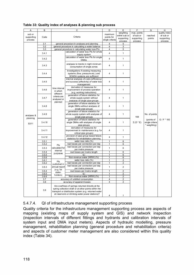
118

Table 33: Quality index of analyses & planning sub process

5.4.7.4. QI of infrastructure management supporting process Quality criteria for the infrastructure management supporting process are aspects of mapping (existing maps of supply system and GIS) and network inspection (inspection intervals of different fittings and hydrants and calibration intervals of system input and DMA input meters). Aspects of hydraulic modelling, pressure management, rehabilitation planning (general procedure and rehabilitation criteria) and aspects of customer meter management are also considered within this quality index (Table 34).

A B D E F G H

sub or supporting

processCode

maximum points for

single criteria

weighting within sub or supporting

process

max. points of sub or

supporting process

reached points

quality index of sub or

supporting process

3.1 4 53.2 4 33.3 4 5

3.4.1 calculation of water loss PIs for whole supply system 4 1

3.4.2calculation of water loss PIs for single

DMAs 4 1

3.4.3analyses to trends in night minimum

consumption of single zones 4 1

3.4.4investigations if existing measuring systems (flow, pressure etc.) and

SCADA systems are sufficient 4 1

3.4.5internal analyses of costs (efficiency) and success (affectivity) of water loss

management4 1

3.4.6derivation of measures for

improvement of process operation (e.g. working instructions)

4 1

3.4.7generation of failure statistics for

whole supply system without analyses of single pipe-groups

4 1

3.4.8generation of failure statistics for single DMAs without analyses of

single pipe-groups4 1

3.4.9generation of failure statistics for

whole supply system with analyses of single pipe-groups

4 1

3.4.10generation of failure statistics for

single DMAs with analyses of single pipe-groups

4 1

3.4.11derivation of measures for

improvement in maintenance (e.g. for critical pipe groups)

4 1

3.4.12 provision of pipe-group based failure statistics for rehabilitation planning 4 1

3.5.1 water loss ratio (%) 1 63.5.2 real losses per connection per day 1 6

3.5.3 real losses per connection per day per metre pressure 1 6

3.5.4 real losses per mains length 1 63.5.5 ILI 1 63.5.6 Non-revenue water (NRW) (%) 1 63.6.1 water loss ratio (%) 1 23.6.2 real losses per connection per day 1 2

3.6.3 real losses per connection per day per metre pressure 1 2

3.6.4 real losses per mains length 1 23.6.5 ILI 1 23.6.6 Non-revenue water (NRW) (%) 1 23.7 4 23.8 4 2

3.9

4 1

G / F * 100

general procedure in calculating water loss PIs

general procedure in analyses and planning

analyses & planning

S311

168

Σ (D * E)

No. of points

(points of single critera * weighting)

Are overflows of springs returned directly at the spring collection shaft or at other points within the

transport or distribution system (e.g. returned water at reservoirs or drinking water power stations)?

time interval in which different

criteria are analysed or

planned

PIs calculated for

internal purposes

PIs published in annual report

(e.g. for stake-

holders)

accuracy of unbilled consumptionaccuracy of apparent losses

C

Criteria

general procedure in calculating a water balance

119

Table 34: Quality index of infrastructure management supporting process

5.4.7.5. QI of leak repair supporting process The quality of the process operation of the leak repair supporting process is mainly expressed by the repair time (time from locating a leak to the recovery of the functionality of the pipe) for distribution mains and service connections and by the modality of failure documentation (Table 35). The information provided by failure documentation is an essential basis for the rehabilitation planning.

Table 35: Quality index of leak repair supporting process

The “product” quality of the repair itself (quality of material used and working quality) is not considered because no serious and comparable data can be expected due to

A B D E F G H

sub or supporting

processCode

maximum points for

single criteria

weighting within sub or supporting

process

max. points of sub or

supporting process

reached points

quality index of sub or

supporting process

4.1 4 54.2.1 4 14.2.2 4 14.2.3 4 14.2.4 4 14.2.5 4 14.3 4 2

4.4 4 1

4.5 4 24.6 4 54.7 4 14.8 4 2

4.9.1 experience of network engineer 1 0,84.9.2 on basis of failure rates 1 0,84.9.3 on basis of water losses 1 0,8

4.9.4 coordination with other construction sites 1 0,8

4.9.5 with special software 1 0,84.10 metering equipment 4 24.11 meter age and replacement interval 4 24.12 time frame for meter readings 4 1

4.13 theft of water, illegal connections, bypasses, manipulations

4 1

general procedure in rehabilitation planning

rehabilitation criteria

inspection interval closing valvesinspection interval hydrants

G / F * 100

C

Criteria

customer meter

management

infrastructure management

H001

Were optimisation potentials in pressure management investigated by hydraulic modelling?

general procedure in pressure managementaverage service pressure headmaximal service pressure head

mapping / GIS

120

Σ (D * E)

No. of points

(points of single critera * weighting)

inspection interval pressure reduction valvescalibration interval system input meters

calibration interval DMA metersaccomplishment of hydraulic modelling

A B D E F G H

sub or supporting

processCode

maximum points for

single criteria

weighting within sub or supporting

process

max. points of sub or

supporting process

reached points

quality index of sub or

supporting process

5.1 4 15.2 4 15.3 4 15.4 4 1

5.5 4 1

5.6 4 15.7 4 1

5.8.1 name of documenting person 1 15.8.2 place and time of failure 1 15.8.3 year of construction 1 15.8.4 pipe diameter 1 1

5.8.5 type of pipe (transportation or distribution main, service connection) 1 1

5.8.6 pipe material 1 15.8.7 pipe connection 1 15.8.8 corrosion protection 1 1

5.8.9 affected part (pipe, fitting, connection) 1 1

5.8.10 condition of pipe and bedding 1 15.8.11 type of failure (burst, fitting…) 1 15.8.12 cause of failure (e.g. corrosion) 1 1

5.8.13 sketch of position, photo documentation 1 1

5.8.14 process of failure elimination 1 15.8.15 type of repair / maintenance 1 15.8.16 costs of repair 1 1

leak repair

H002

information for maintenance and rehabilitation planning

44

Σ (D * E)

No. of points

(points of single critera * weighting)

G / F * 100

modality of failure documentation

criteria of failure docu-

mentation

(according to OVGW

guidelineW 100)

Does it happen that leaks are located but repaired weeks or month later?

C

Criteria

repair time for reported leaks at distribution mainsrepair time for unreported leaks at distribution mainsrepair time for reported leaks at service connections

repair time for unreported leaks at service connections

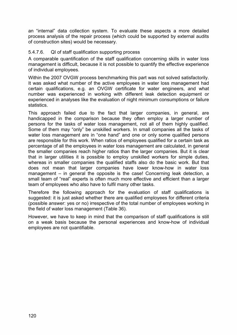
120

an “internal” data collection system. To evaluate these aspects a more detailed process analysis of the repair process (which could be supported by external audits of construction sites) would be necessary.

5.4.7.6. QI of staff qualification supporting process A comparable quantification of the staff qualification concerning skills in water loss management is difficult, because it is not possible to quantify the effective experience of individual employees. Within the 2007 OVGW process benchmarking this part was not solved satisfactorily. It was asked what number of the active employees in water loss management had certain qualifications, e.g. an OVGW certificate for water engineers, and what number was experienced in working with different leak detection equipment or experienced in analyses like the evaluation of night minimum consumptions or failure statistics. This approach failed due to the fact that larger companies, in general, are handicapped in the comparison because they often employ a larger number of persons for the tasks of water loss management, not all of them highly qualified. Some of them may “only” be unskilled workers. In small companies all the tasks of water loss management are in “one hand” and one or only some qualified persons are responsible for this work. When ratios of employees qualified for a certain task as percentage of all the employees in water loss management are calculated, in general the smaller companies reach higher ratios than the larger companies. But it is clear that in larger utilities it is possible to employ unskilled workers for simple duties, whereas in smaller companies the qualified staffs also do the basic work. But that does not mean that larger companies have lower know-how in water loss management – in general the opposite is the case! Concerning leak detection, a small team of “real” experts is often much more effective and efficient than a larger team of employees who also have to fulfil many other tasks. Therefore the following approach for the evaluation of staff qualifications is suggested: it is just asked whether there are qualified employees for different criteria (possible answer: yes or no) irrespective of the total number of employees working in the field of water loss management (Table 36). However, we have to keep in mind that the comparison of staff qualifications is still on a weak basis because the personal experiences and know-how of individual employees are not quantifiable.

121

Table 36: Quality index of staff qualification supporting process

5.4.7.7. QI of the main process The quality index of the main process is calculated by weighting the single quality indices of the sub and supporting processes. Of course this “overall quality performance” has to be seen critically, because a lot of (sometimes) soft single criteria, which are weighted within the sub quality indices, are behind this value. These sub indices are then weighted for the calculation of the main process quality index. Anyone who has ever worked with weightings knows that weightings are not always 100% objective and others may define other weightings. The experiences with the 2007 OVGW process benchmarking show that the weightings used and the criteria considered may not lead to the full truth (Table 37). In chapter 6.3, the problems that occurred with the quality index are described. The missing consideration of water loss PIs was identified as the main problem. For some utilities, the quality performance did not correlate with their water loss PIs, which means that although the water losses are of a medium or high level, a high level in process quality is reached. Therefore it can be disputed that the right questions were asked for the quality assessment and the weightings for the quality index calculation were correct. Further, the consideration of water loss PIs also seems to be necessary. The quality index in Table 38 represents an adapted version with adjusted weighting but also with the consideration of the amount of water losses in form of the ILI. Nevertheless it is recommended to be cautious in using the main process quality

A B C D E F G H

sub or supporting

processCode Criteria

maximum points for

single criteria

weighting within sub or supporting

process

max. points of sub or

supporting process

reached points

quality index of sub or

supporting process

6.1 employees who are proved water engineers (y/n) 1 2

6.2employees with special training

course an water loss management (y/n)

1 2

6.3employees with experience in using listening sticks and stethoscopes

(y/n)1 2

6.4 employees with experience in using ground microphones (y/n) 1 2

6.5 employees with experience in using leak noise correlators (y/n) 1 2

6.6 employees with experience in using noise loggers (y/n) 1 2

6.7 employees with experience in using tracer gas (y/n) 1 2

6.8employees with experience in evaluation of zonal (or DMA)

measurements (y/n)1 2

6.9employees with experience in evaluation of night minimum

consumption (y/n)1 2

6.10 employees with experience in pipe group based failure statistics (y/n) 1 2

6.11 operation of hydraulic modelling with own staff (y/n) 1 2

6.12 procedure in advanced staff training 4 1

qualification of staff

26

Σ (D * E)

No. of points

(points of single critera * weighting)

G / F * 100

122

index. Instead of the main process quality index only the single quality indices of the sub and supporting processes should be used for quality assessment.

Table 37: Quality index of 2007 OVGW process benchmarking

Table 38: Quality index main process (adapted)

A B C D E F

sub or supporting process type of process

quality index of sub or

supporting process(PI No.)

weighting of sub or

supporting process

max. points of sub or

supporting process

reached points of sub or supporting

process

leakage monitoring S111 2 2 C * D

leak detection S211 2 2 C * D

analyses & planning S311 2 2 C * D

infrastructure management H001 1 1 C * D

leak repair H002 2 2 C * D

qualification of staff H003 1 1 C * D

sum ∑E(max. 10)

∑F

quality index main processM11

sub process

supporting process

∑F / ∑E

A B C D E F

sub or supporting process type of process

quality index of sub or

supporting process(PI No.)

weighting of sub or

supporting process

max. points of sub or

supporting process

reached points of sub or supporting

process

leakage monitoring S111 4 4 C * D

leak detection S211 4 4 C * D

analyses & planning S311 3 3 C * D

infrastructure management H001 3 3 C * D

leak repair H002 2 2 C * D

qualification of staff H003 1 1 C * D

ILIcategories A (3 points) - D (0 points) Wl05 3 9 C * D

sum ∑E(max. 26) ∑F

quality index main processM11

sub process

supporting process

∑F / ∑E

123

5.5. The Process Quality Matrix The quality indices described in the previous chapter represent highly aggregated indices which are not very transparent on a first view. Therefore the derivation of measures directly on the basis of these indices is not possible. For the purposes of transparency regarding the individual criteria which lay behind the indices, but more for obtaining an overview about strengths and weaknesses in process operation, a process quality matrix was developed. The idea of this quality matrix is to give a fast overview of optimisation potentials. Therefore each of the single criteria of the matrix is categorised into five different performance levels (from low to high). The different performance levels are indicated by different colours within the matrix (Table 39). Some questions are answered by “yes” (light blue) or “no” (red), and some questions enable more than one answer (e.g. leak detection equipment, 2.6 in Table 41). In these cases those fields which are accepted as “true” are indicated by a dark green colour.

Table 39: Indication of performance levels in the quality matrix

performance level colour 1 low performance red 2 orange 3 medium performance yellow 4 green 5 high performance light blue

equivalent answers (for questions with more than one possible answer) dark green (answer: true or yes)

The whole quality matrix is split into six tables (Table 40 to Table 45) due to the lack of space. The individual criteria are equal to the criteria for the quality indices in Table 31 to Table 36, but here also the possible answers (of the participating water supply utilities) are shown in detail.

124

Table 40: Quality matrix for leakage monitoring sub process (part 1)

low

med

ium

high

red

oran

geye

llow

gree

nlig

ht b

lue

12

34

51 1.1

syst

em in

put m

eter

ing

Mos

t of o

ur s

yste

m in

put i

s no

t met

ered

Not

all,

but

> 5

0% o

f our

sy

stem

inpu

t is

met

ered

Our

sys

tem

inpu

t is

met

ered

bu

t we

are

not s

ure

abou

t the

ac

cura

cy o

f the

se (p

artly

old

) m

eter

s

Our

sys

tem

inpu

t is

met

ered

w

ith m

echa

nica

l and

/or

mag

netic

flow

met

ers

that

are

ra

rely

cal

ibra

ted

Our

sys

tem

inpu

t is

met

ered

w

ith m

agne

tic fl

ow m

eter

s th

at a

re re

gula

rly c

alib

rate

d

1.2

dist

rict

met

ered

are

as

(DM

A)W

e ha

ve n

o D

MA

s an

d ha

ve

no p

lans

to e

stab

lish

DM

As

We

plan

to in

stal

l DM

As

and

have

sta

rted

to e

stab

lish

the

first

DM

As

The

first

DM

As

are

esta

blis

hed

and

we

have

al

read

y th

e fir

st re

sults

We

have

sev

eral

DM

As

and

chec

k an

d an

alys

e in

flow

dat

a sp

orad

ical

ly

We

have

sev

eral

DM

As

and

mon

itor f

low

and

pre

ssur

e on

a

regu

lar b

asis

1.3

eval

uatio

n of

nig

ht

min

imum

con

sum

ptio

n

Up

to n

ow w

e di

d no

t eva

luat

e th

e ni

ght m

inim

um

cons

umpt

ion

The

nigh

t min

imum

co

nsum

ptio

n is

met

ered

and

an

alys

ed s

pora

dica

lly w

ith

exte

rnal

inst

rum

ents

The

nigh

t min

imum

co

nsum

ptio

n is

met

ered

dai

ly

but e

valu

ated

onl

y in

larg

er

inte

rval

ls (e

.g. o

nce

in a

wee

k or

mon

th)

We

anal

yse

the

nigh

t m

inim

um c

onsu

mpt

ion

of th

e w

hole

sys

tem

eve

ry d

ay

We

anal

yse

the

nigh

t m

inim

um c

onsu

mpt

ion

of

each

DM

A e

very

day

1.4

SCAD

A sy

stem

(SC

ADA

)W

e do

not

hav

e a

SC

AD

A

syst

emW

e ha

ve s

tarte

d to

pla

n (o

r in

stal

l) a

SC

AD

A s

yste

m

We

have

a S

CA

DA

sys

tem

bu

t not

all

of o

ur s

yste

m in

put

met

ers

or z

onal

met

ers

are

impl

emen

ted

All

of o

ur s

yste

m in

put m

eter

da

ta o

r zon

al m

eter

dat

a ar

e tra

nsm

itted

to a

con

trol r

oom

pe

rman

ently

All

of o

ur s

yste

m in

put m

eter

da

ta o

r zon

al m

eter

dat

a ar

e tra

nsm

itted

to a

con

trol r

oom

pe

rman

ently

and

ther

e ar

e au

tom

atic

ala

rms

if lim

its a

re

exce

eded

1.4.

1fu

nctio

ns o

f SC

ADA

syst

em(m

ore

than

1 a

nsw

er

poss

ible

)

Tran

smis

sion

of s

yste

m in

put

data

(spr

ings

, wel

ls)

Tran

smis

sion

of z

onal

inpu

t da

ta (D

MA

inpu

ts)

Tran

smis

sion

of p

ress

ure

mea

sure

men

tsTr

ansm

issi

on o

f wat

er le

vels

in

rese

rvoi

rsTr

ansm

issi

on o

f flo

ws

of

pum

ping

sta

tions

1.4.

1.1

data

tran

smis

sion

inte

rval

sy

stem

inpu

t dat

aon

ce a

day

or l

ess

>15

min

.1-

15 m

in.

each

min

ute

perm

anen

t

1.4.

1.2

data

tran

smis

sion

inte

rval

D

MA

inpu

t dat

aon

ce a

day

or l

ess

>15

min

.1-

15 m

in.

each

min

ute

perm

anen

t

1.4.

1.3

data

tran

smis

sion

inte

rval

pr

essu

re d

ata

once

a d

ay o

r les

s>1

5 m

in.

1-15

min

.ea

ch m

inut

epe

rman

ent

1.4.

1.4

data

tran

smis

sion

inte

rval

re

serv

oir l

evel

once

a d

ay o

r les

s>1

5 m

in.

1-15

min

.ea

ch m

inut

epe

rman

ent

1.4.

1.5

data

tran

smis

sion

inte

rval

pu

mpi

ng s

tatio

n da

taon

ce a

day

or l

ess

>15

min

.1-

15 m

in.

each

min

ute

perm

anen

t

1.4.

2

1.4.

3

topi

cqu

estio

n

perf

orm

ance

leve

l

sub

proc

ess

leak

age

mon

itorin

g (p

art 1

)

auto

mat

ed e

valu

atio

n of

nig

ht m

inim

um c

onsu

mpt

ion

noye

s

auto

mat

ed a

larm

whe

n tre

shol

ds e

xcee

ded

(e.g

. inc

reas

e in

sys

tem

inpu

t or d

ecre

ase

of s

ervic

e pr

essu

re)

noye

s

125

Table 40 continued: Quality matrix for leakage monitoring sub process (part 2)

low

med

ium

high

red

oran

geye

llow

gree

nlig

ht b

lue

12

34

51 1.5

pres

sure

mon

itorin

gW

e do

not

hav

e an

y pr

essu

re

mon

itorin

g sy

stem

s in

stal

led

We

have

a fe

w p

ress

ure

mon

itorin

g sy

stem

s at

pum

ping

st

atio

ns a

nd tr

eatm

ent p

lant

s

We

have

a fe

w p

ress

ure

mon

itorin

g sy

stem

s at

pum

ping

st

atio

ns a

nd tr

eatm

ent p

lant

s an

d sp

orad

ical

ly w

e m

easu

re

the

pres

sure

with

in th

e di

strib

utio

n sy

stem

(with

mob

ile

man

omet

ers)

We

have

a fe

w p

ress

ure

mon

itorin

g sy

stem

s at

pum

ping

st

atio

ns a

nd tr

eatm

ent p

lant

s an

d sp

orad

ical

ly w

e m

easu

re

the

pres

sure

with

in th

e di

strib

utio

n sy

stem

with

pr

essu

re lo

gger

s

We

have

per

man

ent i

nsta

lled

pres

sure

logg

ers

and

reco

rd

the

pres

sure

with

in th

e di

strib

utio

n sy

stem

co

ntin

uous

ly

1.6

perm

anen

t noi

se lo

gger

s

We

do n

ot h

ave

any

perm

anen

t noi

se lo

gger

s an

d w

e w

ill no

t use

suc

h lo

gger

s in

th

e fu

ture

At th

e m

omen

t we

do n

ot h

ave

any

perm

anen

t noi

se lo

gger

s bu

t may

be

we

will

use

suc

h lo

gger

s in

the

futu

re

We

have

a fe

w p

erm

anen

t no

ise

logg

ers

but w

e do

not

th

ink

abou

t an

area

-wid

e us

e

We

have

sta

rted

with

an

area

-w

ide

use

of p

erm

anen

t noi

se

logg

ers

in s

ome

dist

ricts

of o

ur

supp

ly s

yste

m a

nd a

im fo

r a

cove

rage

of t

he w

hole

di

strib

utio

n sy

stem

We

have

an

area

-wid

e us

e of

pe

rman

ent n

oise

logg

ers

in o

ur

dist

ribut

ion

syst

em a

nd

eval

uate

noi

se d

ata

regu

larly

(s

ever

al ti

mes

a y

ear)

1.7

virt

ual m

easu

ring

zone

sW

e do

not

hav

e a

leak

age

mon

itorin

g in

larg

e zo

nes

In p

arts

of o

ur s

uppl

y sy

stem

w

e st

arte

d to

impl

emen

t virt

ual

mea

siru

ng z

ones

(by

flow

m

easu

rem

ents

onl

y)

In p

arts

of o

ur s

uppl

y sy

stem

w

e st

arte

d to

impl

emen

t virt

ual

mea

siru

ng z

ones

usi

ng

mul

itpar

amet

er m

easu

rem

ents

We

have

an

area

-wid

e sy

stem

of

virt

ual m

easu

ring

zone

s bu

t w

e us

e on

ly fl

ow

mea

sure

men

ts

We

have

an

area

-wid

e us

e of

m

ultip

aram

eter

mea

sure

men

ts

in o

ur d

istri

butio

n sy

stem

with

an

aut

omat

ical

leak

det

ectio

n so

ftwar

e

1.8

reco

gniti

on o

f lea

kage

We

only

get

aw

are

of b

urst

s w

hen

the

rese

rvoi

r is

sudd

enly

em

pty,

sin

gle

smal

l lea

k ar

e no

t rec

ogni

sed

Exis

ting

leak

s w

hich

do

not

com

e to

the

surfa

ce a

re o

nly

reco

gnis

ed in

the

cour

se o

f le

ak d

etec

tion

cam

paig

ns

Exis

ting

leak

s w

hich

do

not

com

e to

the

surfa

ce a

re

reco

gnis

ed o

n ba

sis

of m

onth

ly

eval

uatio

ns o

f the

sys

tem

inpu

t vo

lum

e

Exis

ting

leak

s w

hich

do

not

com

e to

the

surfa

ce a

re

reco

gnis

ed o

n ba

sis

of w

eekl

y ev

alua

tions

of t

he s

yste

m in

put

volu

me

Beca

use

of d

aily

nig

ht

min

imum

con

sum

ptio

n ev

alua

tions

als

o sm

alle

r lea

ks

are

reco

gnis

ed w

ithin

24

hour

s

1.9

first

info

rmat

ion

abou

t lea

k lo

catio

n

With

the

exis

ting

leak

age

mon

itorin

g sy

stem

it is

not

po

ssib

le to

get

any

info

rmat

ion

abou

t the

loca

tion

of a

leak

Just

a ro

ugh

estim

atio

n in

wha

t di

stric

t of t

he s

uppl

y sy

stem

th

e le

ak is

loca

ted

is a

vaila

ble

With

our

leak

age

mon

itorin

g sy

stem

bur

sts

can

be

spat

ialis

ed to

sin

gle

DM

As

With

our

leak

age

mon

itorin

g sy

stem

bur

sts

can

be

spat

ialis

ed to

pip

e se

ctio

ns

with

less

than

1.0

00 m

leng

ht

(with

out a

dditi

onal

leak

de

tect

ion

mea

sure

s)

With

our

leak

age

mon

itorin

g sy

stem

bur

sts

can

be

spat

ialis

ed to

pip

e se

ctio

ns

with

less

than

300

m le

nght

(w

ithou

t add

ition

al le

ak

dete

ctio

n m

easu

res)

1.10

accu

racy

of s

yste

m in

put

met

erin

g+/

- >1

00%

+/-

25-1

00%

+/-

5-25

%+/

- 2-

5%+/

- 2%

1.11

max

. zon

e si

ze (a

ccor

ding

m

ains

leng

th)

> 50

0 km

100-

500

km50

-100

km

25-5

0 km

< 25

km

1.12

max

. zon

e si

ze (a

ccor

ding

N

o. o

f ser

vice

con

nect

ions

)>

50.0

00 s

ervi

ce c

onne

ctio

ns10

.000

-50.

000

serv

ice

conn

ectio

ns3.

000-

10.0

00 s

ervi

ce

conn

ectio

ns1.

000-

3.00

0 se

rvic

e co

nnec

tions

< 1.

000

serv

ice

conn

ectio

ns

1.13

aver

age

zone

siz

e (w

eigh

ted

onto

No.

of s

ervi

ce

conn

ectio

ns)

> 10

.000

ser

vice

con

nect

ions

3.00

0-10

.000

ser

vice

co

nnec

tions

1.00

0-3.

000

serv

ice

conn

ectio

ns50

0-1.

000

serv

ice

conn

ectio

ns<

500

serv

ice

conn

ectio

ns

1.14

aver

age

zone

siz

e (w

eigh

ted

onto

mai

ns le

ngth

)>

200

km10

0-20

0 km

50-1

00 k

m25

-50

km<

25 k

m

1.15

port

ion

of D

MA

of w

hole

su

pply

sys

tem

(acc

ordi

ng

mai

ns le

ngth

)0%

0% to

30%

30%

to 7

0%70

% to

100

%10

0%

topi

cqu

estio

n

perf

orm

ance

leve

l

sub

proc

ess

leak

age

mon

itorin

g (p

art 2

)

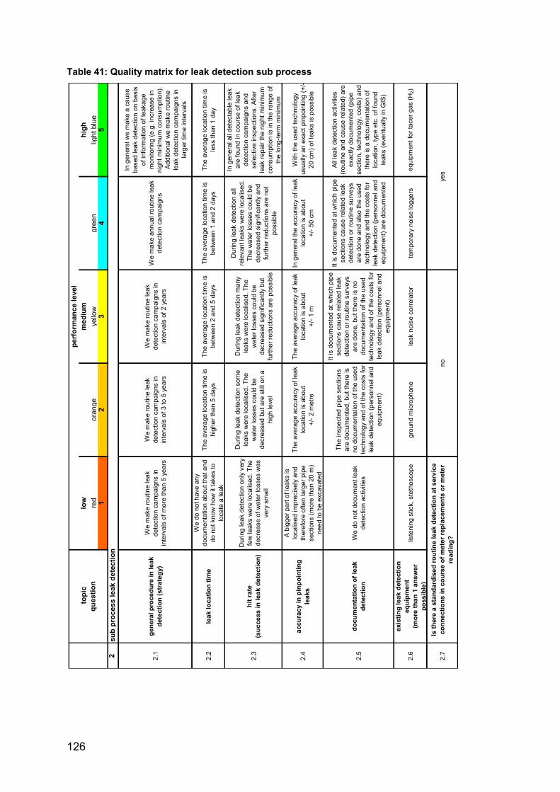
126

Table 41: Quality matrix for leak detection sub process

low

med

ium

high

red

oran

geye

llow

gree

nlig

ht b

lue

12

34

52 2.1

gene

ral p

roce

dure

in le

ak

dete

ctio

n (s

trat

egy)

We

mak

e ro

utin

e le

ak

dete

ctio

n ca

mpa

igns

in

inte

rval

s of

mor

e th

an 5

yea

rs

We

mak

e ro

utin

e le

ak

dete

ctio

n ca

mpa

igns

in

inte

rval

s of

3 to

5 y

ears

We

mak

e ro

utin

e le

ak

dete

ctio

n ca

mpa

igns

in

inte

rval

s of

2 y

ears

We

mak

e an

nual

rout

ine

leak

de

tect

ion

cam

paig

ns

In g

ener

al w

e m

ake

a ca

use

base

d le

ak d

etec

tion

on b

asis

of

info

rmat

ion

of le

akag

e m

onito

ring

(e.g

. inc

reas

e in

ni

ght m

inim

um c

onsu

mpt

ion)

. Ad

ditio

nal w

e m

ake

rout

ine

leak

det

ectio

n ca

mpa

igns

in

larg

er ti

me

inte

rval

s

2.2

leak

loca

tion

time

We

do n

ot h

ave

any

docu

men

tatio

n ab

out t

hat a

nd

do n

ot k

now

how

it ta

kes

to

loca

te a

leak

The

aver

age

loca

tion

time

is

high

er th

an 5

day

sTh

e av

erag

e lo

catio

n tim

e is

be

twee

n 2

and

5 da

ysTh

e av

erag

e lo

catio

n tim

e is

be

twee

n 1

and

2 da

ysTh

e av

erag

e lo

catio

n tim

e is

le

ss th

an 1

day

2.3

hit r

ate

(suc

cess

in le

ak d

etec

tion)

Dur

ing

leak

det

ectio

n on

ly v

ery

few

leak

s w

ere

loca

lised

. The

de

crea

se o

f wat

er lo

sses

was

ve

ry s

mal

l

Dur

ing

leak

det

ectio

n so

me

leak

s w

ere

loca

lised

. The

w

ater

loss

es c

ould

be

decr

ease

d bu

t are

stil

l on

a hi

gh le

vel

Dur

ing

leak

det

ectio

n m

any

leak

s w

ere

loca

lised

. The

w

ater

loss

es c

ould

be

decr

ease

d si

gnifi

cant

ly b

ut

furth

er re

duct

ions

are

pos

sibl

e

Dur

ing

leak

det

ectio

n al

l re

leva

nt le

aks

wer

e lo

calis

ed.

The

wat

er lo

sses

cou

ld b

e de

crea

sed

sign

ifica

ntly

and

fu

rther

redu

ctio

ns a

re n

ot

poss

ible

In g

ener

al a

ll de

tect

able

leak

ar

e fo

und

in c

ours

e of

leak

de

tect

ion

cam

paig

ns a

nd

sele

ctiv

e in

spec

tions

. Afte

r le

ak re

pair

the

nigh

t min

imum

co

nsum

ptio

n is

in th

e ra

nge

of

the

long

-term

min

imum

2.4

accu

racy

in p

inpo

intin

g le

aks

A bi

gger

par

t of l

eaks

is

loca

lised

impr

ecis

ely

and

ther

efor

e of

ten

larg

er p

ipe

sect

ions

(mor

e th

an 2

0 m

) ne

ed to

be

exca

vate

d

The

aver

age

accu

racy

of l

eak

loca

tion

is a

bout

+/

- 2 m

etre

The

aver

age

accu

racy

of l

eak

loca

tion

is a

bout

+/

- 1 m

In g

ener

al th

e ac

cura

cy o

f lea

k lo

catio

n is

abo

ut

+/- 5

0 cm

With

the

used

tech

nolo

gy

usua

lly a

n ex

act p

inpo

intin

g (+

/-20

cm

) of l

eaks

is p

ossi

ble

2.5

docu

men

tatio

n of

leak

de

tect

ion

We

do n

ot d

ocum

ent l

eak

dete

ctio

n ac

tiviti

es

The

insp

ecte

d pi

pe s

ectio

ns

are

docu

men

ted,

but

ther

e is

no

doc

umen

tatio

n of

the

used

te

chno

logy

and

of t

he c

osts

for

leak

det

ectio

n (p

erso

nnel

and

eq

uipm

ent)

It is

doc

umen

ted

at w

hich

pip

e se

ctio

ns c

ause

rela

ted

leak

de

tect

ion

or ro

utin

e su

rvey

s ar

e do

ne, b

ut th

ere

is n

o do

cum

enta

tion

of th

e us

ed

tech

nolo

gy a

nd o

f the

cos

ts fo

r le

ak d

etec

tion

(per

sonn

el a

nd

equi

pmen

t)

It is

doc

umen

ted

at w

hich

pip

e se

ctio

ns c

ause

rela

ted

leak

de

tect

ion

or ro

utin

e su

rvey

s ar

e do

ne a

nd a

lso

the

used

te

chno

logy

and

the

cost

s fo

r le

ak d

etec

tion

(per

sonn

el a

nd

equi

pmen

t) ar

e do

cum

ente

d

All l

eak

dete

ctio

n ac

tiviti

es

(rou

tine

and

caus

e re

late

d) a

re

exac

tly d

ocum

ente

d (p

ipe

sect

ion,

tech

nolo

gy, c

osts

) and

th

ere

is a

doc

umen

tatio

n of

lo

catio

n, ty

pe e

tc. o

f fou

nd

leak

s (e

vent

ually

in G

IS)

2.6

exis

ting

leak

det

ectio

n eq

uipm

ent

(mor

e th

an 1

ans

wer

po

ssib

le)

liste

ning

stic

k, s

teth

osco

pegr

ound

mic

roph

one

leak

noi

se c

orre

lato

rte

mpo

rary

noi

se lo

gger

seq

uipm

ent f

or ta

cer g

as (H

2)

2.7

topi

cqu

estio

n

perf

orm

ance

leve

l

sub

proc

ess

leak

det

ectio

n

Is th

ere

a st

anda

rdis

ed ro

utin

e le

ak d

etec

tion

at s

ervi

ce

conn

ectio

ns in

cou

rse

of m

eter

repl

acem

ents

or m

eter

re

adin

g?no

yes

127

Table 42: Quality matrix for analyses & planning sub process (part 1)

low

med

ium

high

red

oran

geye

llow

gree

nlig

ht b

lue

12

34

53 3.1

gene

ral p

roce

dure

in

anal

yses

and

pla

nnin

g

We

do n

ot m

ake

any

anal

yses

ac

cord

ing

wat

er lo

ss

man

agem

ent

The

anal

yses

are

lim

ited

to th

e ca

lcul

atio

n of

an

annu

al w

ater

ba

lanc

e

The

anal

yses

are

lim

ited

to th

e ca

lcul

atio

n of

an

annu

al w

ater

ba

lanc

e an

d of

var

ious

wat

er

loss

PIs

We

calc

ulat

e a

wat

er b

alan

ce

and

vario

us w

ater

loss

PIs

an

nual

y. A

naly

ses

of th

e w

ater

lo

ss m

anag

emen

t its

elf w

ith

deriv

atio

n of

opt

imis

atio

n m

easu

res

are

done

in la

rger

tim

e in

terv

als

Besi

de c

alcu

latio

n of

a w

ater

ba

lanc

e an

d w

ater

loss

PIs

we

anal

yse

the

proc

ess

of w

ater

lo

ss m

anag

emen

t (co

st-b

enef

it an

alys

es, r

ehab

ilitat

ion

plan

ning

etc

.) an

d if

nece

ssar

y op

timis

atio

ns a

re im

plem

ente

d

3.2

gene

ral p

roce

dure

in

calc

ulat

ing

a w

ater

bal

ance

Up

to n

ow w

e di

d no

t cal

cula

te

a w

ater

bal

ance

We

tried

to c

alcu

late

a w

ater

ba

lanc

e bu

t had

to g

ive

up,

beca

use

we

do n

ot m

easu

re

the

syst

em in

put

Up

to n

ow w

e ca

lcul

ated

a

wat

er b

alan

ce o

f an

othe

r sc

hem

e th

an th

e IW

A w

ater

ba

lanc

e

We

alre

ady

use

the

IWA

wat

er

bala

nce

for a

n an

nual

ca

lcul

atio

n

We

alre

ady

use

the

IWA

wat

er

bala

nce

for a

n an

nual

ca

lcul

atio

n an

d us

e co

nfid

ence

in

terv

als

to e

stim

ate

the

accu

racy

of w

ater

bal

ance

dat

a

3.3

gene

ral p

roce

dure

in

calc

ulat

ing

wat

er lo

ss P

IsU

p to

now

we

did

not c

alcu

late

w

ater

loss

PIs

The

only

PI w

e ca

lcul

ate

is th

e w

ater

loss

ratio

(%)

We

calc

ulat

e va

rious

tech

nica

l w

ater

loss

PIs

regu

larly

We

calc

ulat

e va

rious

tech

nica

l an

d ec

onom

ical

wat

er lo

ss P

Is

regu

larly

(e.g

. re

al lo

sses

per

m

ains

leng

th, I

LI, r

eal l

osse

s pe

r con

nect

ion

per d

ay, n

on-

reve

nue

wat

er)

We

calc

ulat

e va

rious

tech

nica

l an

d ec

onom

ical

wat

er lo

ss P

Is

regu

larly

(e.g

. IL

I, re

al lo

sses

pe

r con

nect

ion

per d

ay, n

on-

reve

nue

wat

er) a

nd p

ublis

h th

e re

sults

e.g

. in

an a

nnua

l rep

ort

3.4

3.4.

1ca

lcul

atio

n of

wat

er lo

ss P

Is

for w

hole

sup

ply

syst

emne

ver d

one

mor

e th

an 5

yea

rs2-

5 ye

ars

ever

y si

x m

onth

or a

nnua

lm

onth

ly o

r qua

terly

3.4.

2ca

lcul

atio

n of

wat

er lo

ss P

Is

for s

ingl

e D

MAs

neve

r don

em

ore

than

5 y

ears

2-5

year

sev

ery

six

mon

th o

r ann

ual

mon

thly

or q

uate

rly

3.4.

3an

alys

es to

tren

ds in

nig

ht

min

imum

con

sum

ptio

n of

si

ngle

zon

es

neve

r don

em

ore

than

5 y

ears

2-5

year

sev

ery

six

mon

th o

r ann

ual

mon

thly

or q

uate

rly

3.4.

4

inve

stig

atio

ns if

exi

stin

g m

easu

ring

syst

ems

(flow

, pr

essu

re e

tc.)

and

SCAD

A sy

stem

s ar

e su

ffici

ent

neve

r don

em

ore

than

5 y

ears

2-5

year

sev

ery

six

mon

th o

r ann

ual

mon

thly

or q

uate

rly

3.4.

5

inte

rnal

ana

lyse

s of

cos

ts

(effi

cien

cy) a

nd s

ucce

ss

(affe

ctiv

ity) o

f wat

er lo

ss

man

agem

ent

neve

r don

em

ore

than

5 y

ears

2-5

year

sev

ery

six

mon

th o

r ann

ual

mon

thly

or q

uate

rly

topi

cqu

estio

n

perf

orm

ance

leve

l

sub

proc

ess

anal

yses

& p

lann

ing

(par

t 1)

time

inte

rval

in w

hich

diff

eren

t crit

eria

are

ana

lyse

d or

pla

nned

128

Table 42 continued: Quality matrix for analyses & planning sub process (part 2)

low

med

ium

high

red

oran

geye

llow

gree

nlig

ht b

lue

12

34

53

3.4.

6

deriv

atio

n of

mea

sure

s fo

r im

prov

emen

t of p

roce

ss

oper

atio

n (e

.g. w

orki

ng

inst

ruct

ions

)

neve

r don

em

ore

than

5 y

ears

2-5

year

sev

ery

six

mon

th o

r ann

ual

mon

thly

or q

uate

rly

3.4.

7

gene

ratio

n of

failu

re

stat

istic

s fo

r who

le s

uppl

y sy

stem

with

out a

naly

ses

of

sin g

le p

ipe-

grou

ps

neve

r don

em

ore

than

5 y

ears

2-5

year

sev

ery

six

mon

th o

r ann

ual

mon

thly

or q

uate

rly

3.4.

8

gene

ratio

n of

failu

re

stat

istic

s fo

r sin

gle

DM

As

with

out a

naly

ses

of s

ingl

e pi

pe-g

roup

s

neve

r don

em

ore

than

5 y

ears

2-5

year

sev

ery

six

mon

th o

r ann

ual

mon

thly

or q

uate

rly

3.4.

9

gene

ratio

n of

failu

re

stat

istic

s fo

r who

le s

uppl

y sy

stem

with

ana

lyse

s of

si

n gle

pip

e-gr

oups

neve

r don

em

ore

than

5 y

ears

2-5

year

sev

ery

six

mon

th o

r ann

ual

mon

thly

or q

uate

rly

3.4.

10

gene

ratio

n of

failu

re

stat

istic

s fo

r sin

gle

DM

As

with

ana

lyse

s of

sin

gle

pipe

-gr

oups

neve

r don

em

ore

than

5 y

ears

2-5

year

sev

ery

six

mon

th o

r ann

ual

mon

thly

or q

uate

rly

3.4.

11de

rivat

ion

of m

easu

res

for

impr

ovem

ent i

n m

aint

enan

ce

(e.g

. for

crit

ical

pip

e gr

oups

)ne

ver d

one

mor

e th

an 5

yea

rs2-

5 ye

ars

ever

y si

x m

onth

or a

nnua

lm

onth

ly o

r qua

terly

3.4.

12pr

ovis

ion

of p

ipe-

grou

p ba

sed

failu

re s

tatis

tics

for

reha

bilit

atio

n pl

anni

ngne

ver d

one

mor

e th

an 5

yea

rs2-

5 ye

ars

ever

y si

x m

onth

or a

nnua

lm

onth

ly o

r qua

terly

wat

er lo

ss ra

tio (%

)re

al lo

sses

per

con

nect

ion

per

day

real

loss

es p

er c

onn.

per

day

pe

r met

re p

ress

ure

real

loss

es p

er m

ains

leng

thIL

IN

on-r

even

ue w

ater

(NR

W) (

%)

wat

er lo

ss ra

tio (%

)re

al lo

sses

per

con

nect

ion

per

day

real

loss

es p

er c

onn.

per

day

pe

r met

re p

ress

ure

real

loss

es p

er m

ains

leng

thIL

IN

on-r

even

ue w

ater

(NR

W) (

%)

3.7

accu

racy

of u

nbill

ed

cons

umpt

ion

+/- 1

00%

+/- 5

0 bi

s 10

0%+/

- 25

bis

50%

+/- 1

0 bi

s 25

%+/

- <=1

0%

3.8

accu

racy

of a

ppar

ent l

osse

s+/

- 100

%+/

- 50

bis

100%

+/- 2

5 bi

s 50

%+/

- 10

bis

25%

+/- <

=10%

3.9

topi

cqu

estio

n

perf

orm

ance

leve

l

3.6

PIs

publ

ishe

d in

ann

ual r

epor

t (e

.g. f

or s

take

-hol

ders

)(m

ore

than

1 a

nsw

er p

ossi

ble)

Are

over

flow

s of

spr

ings

retu

rned

dire

ctly

at t

he s

prin

g co

llect

ion

shaf

t or a

t oth

er p

oint

s w

ithin

the

supp

ly s

yste

m

(e.g

. ret

urne

d w

ater

at r

eser

voirs

or p

ower

sta

tions

)?re

turn

ed a

t poi

nt w

ithin

the

trans

port

or d

istri

butio

n sy

stem

retu

rned

at s

prin

g co

llect

ion

shaf

t

3.5

PIs

calc

ulat

ed fo

r int

erna

l pur

pose

s(m

ore

than

1 a

nsw

er p

ossi

ble)

sub

proc

ess

anal

yses

& p

lann

ing

(par

t 2)

129

Table 43: Quality matrix for infrastructure management supporting process (part 1)

low

med

ium

high

red

oran

geye

llow

gree

nlig

ht b

lue

12

34

54 4.1

map

ping

/ G

ISW

e do

not

hav

e m

aps

of o

ur

wat

er s

uppl

y sy

stem

The

exis

ting

map

s ar

e no

t up

date

dO

ur m

aps

are

upda

ted

but n

ot

impl

emen

ted

into

a G

IS

Our

map

s ar

e up

date

d bu

t up

to n

ow o

nly

a pa

rt of

it is

im

plem

ente

d in

to a

GIS

We

have

a G

IS b

ased

m

appi

ng w

hich

is re

gula

rly

upda

ted

4.2

4.2.

1in

spec

tion

inte

rval

clo

sing

va

lves

no in

spec

tion

(or c

alib

ratio

n)

plan

ed6

to 1

0 ye

ars

3 to

5 y

ears

1 to

2 y

ears

ever

y si

x m

onth

or m

ore

ofte

n

4.2.

2in

spec

tion

inte

rval

hyd

rant

sno

insp

ectio

n (o

r cal

ibra

tion)

pl

aned

6 to

10

year

s3

to 5

yea

rs1

to 2

yea

rsev

ery

six

mon

th o

r mor

e of

ten

4.2.

3in

spec

tion

inte

rval

pre

ssur

e re

duct

ion

valv

esno

insp

ectio

n (o

r cal

ibra

tion)

pl

aned

6 to

10

year

s3

to 5

yea

rs1

to 2

yea

rsev

ery

six

mon

th o

r mor

e of

ten

4.2.

4ca

libra

tion

inte

rval

sys

tem

in

put m

eter

sno

insp

ectio

n (o

r cal

ibra

tion)

pl

aned

6 to

10

year

s3

to 5

yea

rs1

to 2

yea

rsev

ery

six

mon

th o

r mor

e of

ten

4.2.

5ca

libra

tion

inte

rval

DM

A m

eter

sno

insp

ectio

n (o

r cal

ibra

tion)

pl

aned

6 to

10

year

s3

to 5

yea

rs1

to 2

yea

rsev

ery

six

mon

th o

r mor

e of

ten

4.3

acco

mpl

ishm

ent o

f hyd

raul

ic

mod

ellin

gU

p to

now

no

hydr

aulic

m

odel

ling

was

car

ried

out

Man

y ye

ars

ago

a hy

drau

lic

mod

ellin

g w

as c

arrie

d ou

tW

e pl

an to

car

ry o

ut a

hy

drau

lic m

odel

ling

soon

We

have

an

actu

al h

ydra

ulic

m

odel

l (m

ax. s

ome

year

s ol

d),

larg

er re

habi

litat

ions

and

ex

pans

ions

are

mod

elle

d be

fore

real

isat

ion

We

do h

ydra

ulic

mod

ellin

g co

ntin

uous

ly (e

.g. e

xpan

sion

s,

reha

bilit

atio

n, h

ydra

ulic

op

timis

atio

ns) a

nd o

ur m

odel

is

upda

ted

cont

inuo

usly

4.4

4.5

gene

ral p

roce

dure

in

pres

sure

man

agem

ent

We

are

unco

ncer

ned

abou

t the

pr

essu

re c

ondi

tions

with

in a

re

supp

ly s

yste

m

The

max

imum

ser

vice

pr

essu

res

are

mor

e th

an 1

0 ba

r but

pre

ssur

e re

duct

ions

ar

e no

t pla

nned

The

max

imum

ser

vice

pr

essu

res

are

betw

een

7 an

d 10

bar

, eve

ntua

lly w

e w

ill re

duce

the

pres

sure

in fu

ture

We

know

abo

ut th

e pr

essu

re

cond

ition

s w

ithin

our

sup

ply

syst

em, o

ptim

isat

ions

are

pl

anne

d bu

t not

fully

im

plem

ente

d ye

t

We

know

abo

ut th

e pr

essu

re

cond

ition

s w

ithin

our

sup

ply

syst

em (e

.g. d

ue to

per

man

ent

or te

mpo

rary

pre

ssur

e m

easu

rem

ents

and

/or

hydr

aulic

mod

ellin

g), w

e ha

ve

redu

ced

the

serv

ice

pres

sure

to

an

acce

ptab

le m

inim

um

4.6

aver

age

serv

ice

pres

sure

he

ad>

75 m

55-7

5 m

45-5

5 m

35-4

5 m

< 35

m

4.7

max

imal

ser

vice

pre

ssur

e he

ad>

90 m

70-9

0 m

50-7

0 m

40-5

0 m

< 40

m

supp

ortin

g pr

oces

s in

fras

truc

ture

man

agem

ent (

part

1)

netw

ork

insp

ectio

n

Wer

e op

timis

atio

n po

tent

ials

in p

ress

ure

man

agem

ent

inve

stig

ated

by

hydr

aulic

mod

ellin

g?no

yes

topi

cqu

estio

n

perf

orm

ance

leve

l

130

Table 43 continued: Quality matrix for infrastructure management supporting process (part 2)

low

med

ium

high

red

oran

geye

llow

gree

nlig

ht b

lue

12

34

54 4.8

gene

ral p

roce

dure

in

reha

bilit

atio

n pl

anni

ng

We

do n

ot h

ave

a re

al

reha

bilit

atio

n pl

anni

ng in

our

ut

ility,

reha

bilta

tions

of p

ipes

an

d ar

mar

ture

s ar

e ca

rrie

d ou

t du

e to

rece

nt o

ccur

renc

es a

nd

if th

e ne

cess

ary

mon

ey is

av

aila

ble

The

mai

n re

habi

litat

ion

crite

ria

is th

e pi

pe a

ge

Reh

abilit

atio

n pl

anni

ng is

don

e on

bas

is o

f fai

lure

rate

s an

d un

der c

onsi

dera

tion

of th

e ex

perie

nce

of th

e ne

twor

k en

gine

er (o

r wat

er m

aste

r)

Reh

abilit

atio

n pl

anni

ng is

don

e on

bas

is o

f fai

lure

rate

s an

d un

der c

onsi

dera

tion

of th

e ex

perie

nce

of th

e ne

twor

k en

gine

er (o

r wat

er m

aste

r), t

he

hydr

aulic

per

form

ance

of p

ipes

an

d w

e try

to u

se s

yner

gies

w

ith c

ombi

ned

cons

truct

ion

site

s (e

.g. g

as p

ipes

)

Reh

abilit

atio

n pl

anni

ng is

su

ppor

ted

by s

peci

al s

oftw

are

and

is d

one

on b

asis

of f

ailu

re

rate

s an

d un

der c

onsi

dera

tion

of th

e ex

perie

nce

of th

e ne

twor

k en

gine

er (o

r wat

er

mas

ter)

, the

hyd

raul

ic

perfo

rman

ce o

f pip

es a

nd w

e try

to u

se s

yner

gies

with

co

mbi

ned

cons

truct

ion

site

s

4.9

reha

bilit

atio

n cr

iteria

(mor

e th

an 1

ans

wer

po

ssib

le)

expe

rienc

e of

net

wor

k en

gine

er (o

r wat

er m

aste

r)fa

ilure

rate

sde

velo

pem

ent o

f wat

er lo

sses

othe

r con

stru

ctio

n si

tes

(e.g

. ga

s pi

pes,

stre

ets)

spec

ial p

ipe

reha

bilit

atio

n so

ftwar

e

4.10

cust

omer

met

erin

g eq

uipm

ent

we

do n

ot h

ave

cust

omer

m

eter

sO

nly

larg

e cu

stom

ers

are

met

ered

We

have

sta

rted

to m

eter

all

cust

omer

s bu

t hav

e no

t co

mpl

eted

this

pro

cess

yet

Nea

rly a

ll cu

stom

ers

are

met

ered

, pub

lic ta

ppin

g po

ints

ar

e no

t met

ered

100%

of o

ur c

usto

mer

s ar

e m

eter

ed

4.11

met

er a

ge a

nd re

plac

emen

t in

terv

al

We

do n

ot h

ave

relia

ble

info

rmat

ion

abou

t the

age

of

cust

omer

met

ers

We

only

cha

nge

met

ers

if th

ey

are

obvi

ousl

y de

fect

A lo

t of t

he c

usto

mer

met

ers

are

olde

r tha

n 10

yea

rs, u

p to

no

w w

e di

d no

t wor

k ou

t a

cust

omer

met

er re

plac

emen

t pr

ogra

mm

e

We

have

a c

usto

mer

met

er

repl

acem

ent p

rogr

amm

e bu

t w

e w

ere

not a

ble

to re

plac

e al

l m

eter

s ol

der t

han

10 y

ears

yet

We

repl

ace

all c

usto

mer

m

eter

s in

5 y

ears

inte

rval

s

4.12

time

fram

e fo

r met

er

read

ings

Met

er re

adin

gs a

re u

nder

take

n ov

er th

e w

hole

yea

r (se

vera

l se

pera

ted

time

perio

ds),

ther

efor

e th

e co

nsum

ptio

n da

ta

can

not b

e re

fere

d ex

act t

o a

spec

ific

valid

atio

n da

te

Met

er re

adin

gs a

re u

nder

take

n ov

er th

e w

hole

yea

r (un

iform

ly

dist

ribut

ed),

ther

efor

e th

e co

nsum

ptio

n da

ta c

an n

ot b

e re

fere

d ex

act t

o a

spec

ific

valid

atio

n da

te

Met

er re

adin

gs a

re u

nder

take

n ov

er a

sho

rt tim

e pe

riod,

whi

ch

is th

e sa

me

each

yea

r

All c

usto

mer

met

ers

are

equi

pped

with

a d

ata

logg

er

whi

ch lo

gs th

e an

nual

co

nsum

ptio

n da

ta a

t a s

peci

fic

valid

atio

n da

te

All c

usto

mer

met

ers

are

equi

pped

with

a d

ata

logg

er

whi

ch lo

gs th

e co

nsum

ptio

n da

ta a

t var

ious

spe

cific

va

lidat

ion

date

s

4.13

thef

t of w

ater

, ille

gal

conn

ectio

ns, b

ypas

ses,

m

anip

ulat

ions

We

did

not m

ake

any

inve

stig

atio

n ab

out t

hese

topi

c an

d ha

ve n

o pr

ogra

mm

es

agai

n th

eft o

f wat

er

Occ

assi

onal

ly il

lega

l co

nnec

tions

are

foun

d

Occ

assi

onal

ly il

lega

l co

nnec

tions

or o

ther

frau

ds

(e.g

. the

ft ou

t of h

ydra

nts)

are

fo

und

We

have

a s

yste

mat

ic

prog

ram

e ag

ains

t ille

gal

conn

ectio

ns

We

have

a s

yste

mat

ic

prog

ram

e ag

ains

t ille

gal

conn

ectio

ns, f

or fi

ndin

g by

pass

es a

nd to

avo

id th

eft o

f w

ater

topi

cqu

estio

n

perf

orm

ance

leve

l

supp

ortin

g pr

oces

s in

fras

truc

ture

man

agem

ent (

part

2)

cust

omer

met

er m

anag

emen

t (cu

stom

er m

eter

ing)

131

Table 44: Quality matrix for leak repair supporting process (part 1)

low

med

ium

high

red

oran

geye

llow

gree

nlig

ht b

lue

12

34

55 5.1

repa

ir tim

e fo

r rep

orte

d le

aks

at d

istr

ibut

ion

mai

ns(ti

me

from

loca

ting

a le

ak to

th

e re

cove

ry o

f the

fu

nctio

nalit

y of

the

pipe

)

We

do n

ot h

ave

any

docu

men

tatio

n of

leak

repa

ir,

ther

efor

e w

e do

not

kno

w h

ow

long

it ta

kes

to re

pair

the

leak

The

aver

age

repa

ir tim

e is

m

ore

than

24

hour

sTh

e av

erag

e re

pair

time

is

betw

een

12 a

nd 2

4 ho

urs

The

aver

age

repa

ir tim

e is

be

twee

n 6

and

12 h

ours

The

aver

age

repa

ir tim

e is

less

th

an 6

hou

rs

5.2

repa

ir tim

e fo

r unr

epor

ted

leak

s at

dis

trib

utio

n m

ains

We

do n

ot h

ave

any

docu

men

tatio

n of

leak

repa

ir,

ther

efor

e w

e do

not

kno

w h

ow

long

it ta

kes

to re

pair

the

leak

The

aver

age

repa

ir tim

e is

m

ore

than

7 d

ays

The

aver

age

repa

ir tim

e is

be

twee

n 3

and

7 da

ysTh

e av

erag

e re

pair

time

is

betw

een

1.5

and

3 da

ysTh

e av

erag

e re

pair

time

is le

ss

than

1.5

day

s

5.3

repa

ir tim

e fo

r rep

orte

d le

aks

at s

ervi

ce c

onne

ctio

ns

We

do n

ot h

ave

any

docu

men

tatio

n of

leak

repa

ir,

ther

efor

e w

e do

not

kno

w h

ow

long

it ta

kes

to re

pair

the

leak

The

aver

age

repa

ir tim

e is

m

ore

than

48

hour

sTh

e av

erag

e re

pair

time

is

betw

een

24 a

nd 4

8 ho

urs

The

aver

age

repa

ir tim

e is

be

twee

n 12

and

24

hour

sTh

e av

erag

e re

pair

time

is le

ss

than

12

hour

s

5.4

repa

ir tim

e fo

r unr

epor

ted

leak

s at

ser

vice

con

nect

ions

We

do n

ot h

ave

any

docu

men

tatio

n of

leak

repa

ir,

ther

efor

e w

e do

not

kno

w h

ow

long

it ta

kes

to re

pair

the

leak

The

aver

age

repa

ir tim

e is

m

ore

than

14

days

The

aver

age

repa

ir tim

e is

be

twee

n 7

and

14 d

ays

The

aver

age

repa

ir tim

e is

be

twee

n 2

and

7 da

ysTh

e av

erag

e re

pair

time

is le

ss

than

2 d

ays

5.5

topi

cqu

estio

n

perf

orm

ance

leve

l

supp

ortin

g pr

oces

s le

ak re

pair

(par

t 1)

Doe

s it

happ

en th

at le

aks

are

loca

ted

but r

epai

red

wee

ks

or m

onth

late

r?ye

sno

132

Table 44 continued: Quality matrix for leak repair supporting process (part 2)

low

med

ium

high

red

oran

geye

llow

gree

nlig

ht b

lue

12

34

55 5.6

gene

ral p

roce

dure

in o

f fa

ilure

doc

umen

tatio

nW

e do

not

doc

umen

t fai

lure

sTh

e on

ly p

ossi

bilit

y to

eva

luat

e th

e nu

mbe

r of f

ailu

res

is to

co

unt t

he re

pair

orde

rs

We

only

hav

e a

very

sim

ple

docu

men

tatio

n w

hich

allo

ws

a cl

assi

ficat

ion

of fa

ilure

s at

m

ains

or a

t ser

vice

co

nnec

tions

We

have

a d

etai

led

failu

re

docu

men

tatio

n (e

.g. l

ocat

ion,

di

amet

er, m

ater

ial,

type

of

failu

re e

tc.)

We

have

a d

etai

led

failu

re

docu

men

tatio

n (e

.g. l

ocat

ion,

di

amet

er, m

ater

ial,

type

of

failu

re e

tc.)

and

the

failu

res

are

impl

emen

ted

into

a G

IS

5.7

info

rmat

ion

for m

aint

enan

ce

and

reha

bilit

atio

n pl

anni

ng

The

info

rmat

ion

abou

t fai

lure

s is

not

con

side

red

in

mai

nten

ance

and

reha

bilit

atio

n pl

anni

ng

The

info

rmat

ion

abou

t fai

lure

s is

onl

y pa

rtwis

e co

nsid

ered

in

mai

nten

ance

and

reha

bilit

atio

n pl

anni

ng

In g

ener

al th

e in

form

atio

n ab

out f

ailu

res

is u

sed

in

reha

bilit

atio

n an

d m

aint

enan

ce

plan

ning

, but

som

etm

es th

e in

form

atio

n is

not

con

side

red

The

info

rmat

ion

abou

t fai

lure

s is

ver

y im

porta

nt fo

r our

re

habi

litat

ion

and

mai

nten

ance

pl

anni

ng.

The

info

rmat

ion

abou

t fai

lure

s is

ver

y im

porta

nt fo

r our

re

habi

litat

ion

and

mai

nten

ance

pl

anni

ng. W

ith s

tand

ardi

sed

proc

edur

es th

e in

form

atio

n is

co

nsid

ered

regu

larly

in

reha

bilit

atio

n an

d m

aint

enan

ce

plan

ning

nam

e of

doc

umen

ting

pers

onpl

ace

and

time

of fa

ilure

year

of c

onst

ruct

ion

pipe

dia

met

er

type

of p

ipe

(tran

spor

tatio

n or

di

strib

utio

n m

ain,

ser

vice

co

nnec

tion)

pipe

mat

eria

lpi

pe c

onne

ctio

nco

rros

ion

prot

ectio

n

affe

cted

par

t (pi

pe, f

ittin

g,

conn

ectio

n)co

nditi

on o

f pip

e an

d be

ddin

gty

pe o

f fai

lure

(bur

st, f

ittin

g…)

caus

e of

failu

re (e

.g. c

orro

sion

)

sket

ch o

f pos

ition

, pho

to

docu

men

tatio

npr

oces

s of

failu

re e

limin

atio

nty

pe o

f rep

air /

mai

nten

ance

cost

s of

repa

ir

supp

ortin

g pr

oces

s le

ak re

pair

(par

t 2)

topi

cqu

estio

n

perf

orm

ance

leve

l

5.8

crite

ria o

f fai

lure

doc

umen

tatio

n

(acc

ordi

ng to

OVG

W g

uide

line

W 1

00)

133

Table 45: Quality matrix for staff qualification supporting process

low

med

ium

high

red

oran

geye

llow

gree

nlig

ht b

lue

12

34

56 6.1

6.2

6.3

6.4

6.5

6.6

6.7

6.8

6.9

6.10

6.11

6.12

proc

edur

e in

adv

ance

d st

aff

trai

ning

We

do n

ot tr

ain

our s

taff

Onc

e in

a w

hile

our

em

ploy

ees

atte

nd s

emin

ars,

inte

rnal

sta

ff tra

inin

g do

not

take

pla

ce o

ften

Som

e of

our

em

ploy

ees

have

at

tend

ed s

ever

al c

ours

es a

nd

sem

inar

s, in

futu

re a

ll of

our

em

ploy

ess

shou

ld a

ttend

fu

rther

edu

catio

n se

min

ars

The

leve

l of e

duca

tion

of o

ur

staf

f is

high

. At l

east

onc

e a

year

eac

h of

our

em

ploy

ess

atte

nds

at c

ours

es, s

emin

ars

or c

onfe

renc

es (e

.g. o

f the

As

soci

atio

n fo

r Gas

and

W

ater

). At

leas

t onc

e a

year

in

tern

al s

taff

train

ings

are

or

gani

sed

The

leve

l of e

duca

tion

of o

ur

staf

f is

very

hig

h. T

o ho

ld th

is

high

leve

l our

em

ploy

ees

atte

nd s

ever

al c

ours

es,

sem

iars

etc

. eac

h ye

ar a

nd

addi

tiona

l int

erna

l tra

inin

gs a

re

orga

nise

d se

vera

l tim

es

Is h

ydra

ulic

mod

ellin

g op

erat

ed w

ith o

wn

pers

onne

l or b

y ex

tern

al c

ompa

nies

?ex

tern

al c

ompa

nyow

n pe

rson

nel

empl

oyee

s w

ith e

xper

ienc

e in

eva

luat

ion

of n

ight

min

imum

co

nsum

ptio

nno

yes

empl

oyee

s w

ith e

xper

ienc

e in

pip

e gr

oup

base

d fa

ilure

st

atis

tics

noye

s

empl

oyee

s w

ith e

xper

ienc

e in

usi

ng tr

acer

gas

noye

s

empl

oyee

s w

ith e

xper

ienc

e in

eva

luat

ion

of z

onal

(or D

MA)

m

easu

rem

ents

noye

s

empl

oyee

s w

ith e

xper

ienc

e in

usi

ng le

ak n

oise

cor

rela

tors

noye

s

empl

oyee

s w

ith e

xper

ienc

e in

usi

ng n

oise

logg

ers

noye

s

empl

oyee

s w

ith e

xper

ienc

e in

usi

ng li

sten

ing

stic

ks a

nd

stet

hosc

opes

noye

s

empl

oyee

s w

ith e

xper

ienc

e in

usi

ng g

roun

d m

icro

phon

esno

yes

empl

oyee

s w

ho a

re p

rove

d w

ater

eng

inee

rsno

yes

empl

oyee

s w

ith s

peci

al tr

aini

ng c

ours

e an

wat

er lo

ss

man

agem

ent

noye

s

topi

cqu

estio

n

perf

orm

ance

leve

l

supp

ortin

g pr

oces

s qu

alifi

catio

n of

sta

ff

134

5.6. Verbal descriptions Beside the “hard facts” in the form of variables and performance indicators, additional verbal descriptions about the process operation of single sub and supporting processes can provide useful information. Of course, it is not possible to build up each single activity of the process operation in a fixed process scheme, and such a fixed process can not claim to be the one and only truth. Therefore verbal descriptions are useful for two aspects:

• to enable a better illustration of the process operation and to support deriving measures for improvements

• to identify common practises which should be implemented into the process benchmarking system

Such verbal descriptions were missing in the OVGW field test, but it was seen that this is essential information which has to be used in later projects.

5.7. Exchange of experiences and derivation of measures for improvement

The objectives of process benchmarking are improvements in the performance of process operation. These improvements can be increases in efficiency but also increases in the quality of the process operation. The process benchmarking described in the previous chapters does not represent the whole solution to achieve these objectives. In fact, this performance indicators and quality criteria system represents the basis for further analyses and for the exchange of experiences with other utilities. Of course, the performance indicators give an overview about strengths and weaknesses of a single utility in operating the process of water loss management. But to derive measures for improvement it is necessary to analyse these results. Therefore the first step after the performance comparison should be utility internal analyses of the results to obtain an overview about their own performance and to identify performance gaps. A plausibility check of the (basis) data should also be done at this stage. Questionable data have to be critically analysed before discussions with other utilities. “Best-in-class” workshops can be a good start for the exchange of experiences with other utilities. The results of the process comparison can be presented to all the participating utilities at these workshops and first analyses not only within the whole field of utilities but also within groups with comparable frame conditions can be carried out. The depth of analyses will vary, depending on the duration of the workshops. Experience within the OVGW project shows that one single workshop day is a good start for exchanging views, but following workshops or discussions and analyses, maybe in smaller groups, or even between two utilities, are often necessary to derive concrete measures for improvement.

135

6. Field test - the 2007 OVGW process benchmarking Between February 2007 and April 2008 the OVGW organised a process benchmarking project for the Austrian water supply sector which was initiated and operated by Graz University of Technology and by University of Natural Resources and Applied Life Sciences Vienna. In fact it was the first process benchmarking in the Austrian water supply sector this project also had the character of a field test. Benchmarking the process of water loss management in that form also represents a worldwide innovation. The successful development of a process benchmarking system and an interesting field test with many important experiences was possible with the support of eleven participating water utilities. But the first trial on benchmarking the process of water loss management was more than just a field test: according to the participants’ feedback the project succeeded in comparing the different procedural methods in water loss management for different structures and sizes of utilities and it was possible to derive measures for improvement.

6.1. Frame conditions The process benchmarking system used in the field test differs in some points from the system described within this thesis. The improvements which were implemented to the system were described in the chapters about the process benchmarking system and are described in chapter 6.3. An assessment period of three years (2004, 2005 and 2006) was used for most of the data to give better comparability. The PIs calculated represent average values of the three years which are broken down on a single year. The water balance and water loss PIs were calculated for the single year 2006. Table 46 gives an overview about the frame conditions and the different strategies in water loss management used by the participating utilities of the 2007 OVGW process benchmarking. The utilities with the numbers 1, 3 and 11 represent rural structures. Utilities 5, 7, 9 and 10 are smaller cities with about 2000 to about 15000 inhabitants. The utilities 2, 4, 6 and 8 are larger cities with about 50000 to 200000 inhabitants.

Table 46: Frame conditions and strategies of participating utilities in 2007 OVGW process benchmarking (part 1)

utility nr. urbanity grouping system

input volumestrategy in leak

detectionexisting DMAs

night minimum monitoring

use of noise loggers

1 rural > 5 Mio. m³/a cause based yes yes no2 large city > 5 Mio. m³/a mixed yes yes no3 rural < 5 Mio. m³/a cause based yes yes no4 large city > 5 Mio. m³/a routine surveys yes yes no5 small city < 5 Mio. m³/a mixed yes yes no6 large city > 5 Mio. m³/a routine surveys planned no no7 small city < 5 Mio. m³/a no strategy yet planned no no8 large city > 5 Mio. m³/a mixed yes yes yes9 small city < 5 Mio. m³/a mixed yes yes yes

10 small city < 5 Mio. m³/a mixed no yes no11 rural < 5 Mio. m³/a cause based planned yes no

136

Table 46 continued: Frame conditions and strategies of participating utilities in 2007 OVGW process benchmarking (part 2)

The urbanity as an indicator for the structure of the water supply system is one of the most important grouping criteria beside the strategy in leak detection (whether this is done cause-based or in form of routine surveys, compare chapter 4.5.3).

6.2. Summary of results In this chapter the most important and most significant results of the 2007 OVGW process benchmarking project in Austria are described. The focus is on project results, which are important from a methodological point of view. The description follows the structure of the PI system, starting with water loss PI, next the results of the main process and afterwards the results of the sub- and supporting processes. Last but not least, results about quality indices and outcomes of the best-practice workshop are explained. Please note that all results shown for the 2007 OVGW process benchmarking are results based on the process benchmarking system used in this OVGW 2007 project. Some adaptations of this process benchmarking system, in particular of the process structure, are described in this thesis (compare chapters 5 and 6.3). These improvements in the process benchmarking system are not reflected within the project results shown! Those results which represent the adapted process benchmarking system with the implemented improvements are indicated clearly.

6.2.1. Water Loss PIs The performance within the water loss PIs shows how successful a water utility operates its water loss management. It also has to be mentioned that it is very important to watch the trend of water loss PIs and not only data of a single year in order to evaluate the success in water loss management. The importance of considering data accuracy of water balance data should also be mentioned. The “min.” and “max.” values in Figure 40 to Figure 44 represent confidence intervals in the form of maximal possible error margins. These error margins are calculated on the basis of the error margins of each single water balance data and the error margins of basic data like mains length, number of service connections or average service pressure head. For the “min.” and “max.” values the best and the worst case for each water loss PI was calculated. Therefore, except for the ILI, the “min.” and “max.” values are symmetric under and above the “directly

utility nr.

routine leak detection at

service connections

dominating pipe material

at service connections

hydraulic modelling

own measuring

vehicle

proportion of distribution mains annually inspected

by leak detection methodologies

service connection

density (conn./km)

average service

pressure head (m)

1 no plastic planned no 0.4% (using DMAs) 27.3 522 yes plastic planned yes 17% 31.4 493 no plastic old no 7.6% (using DMAs) 21.3 544 no plastic & metal planned no 107% 30.4 405 no plastic & metal actual no 36% 28.7 506 yes plastic actual yes 27% 29.9 407 no plastic planned no 9.5% 36.3 508 yes plastic actual yes 101% 38.3 449 no metal actual no 117% 21.4 60

10 yes plastic old no 53% 23.3 5011 yes plastic actual no 1.8% (using DMAs) 34.7 55

137

calculated” value, which is calculated directly from the input data. Experience shows that the “right” value usually is anywhere between the directly calculated value and the maximum value because over registration normally does not occur at system input meters. Therefore the system input volume tends to be underestimated what leads to an underestimation of real losses. Small error margins for the system input volume can also lead to high error margins for the volume of real water losses when the real losses are at a low level, some of values of single utilities have error margins of about 100 % or even more: e.g., utility number 3 and utility number 8. The water loss ratio (Figure 40) represents the percentages of the real losses of the system input. This PI is still very common although it is definitely not qualified for the assessment of water losses (compare chapter 4.4.1). But this PI is calculated within the process benchmarking project to show the unserviceableness in comparison with other PIs.

Figure 40: Water loss ratio (source: 2007 OVGW process benchmarking in KOELBL et al. 2008a)

For the technical assessment of water losses it is necessary to use PIs which consider structural parameters like the mains length, the number of service connections or the average service pressure. In DVGW W 392 (2003), real losses per mains length are the decisive PI whereby an assessment subject to the structure of the distribution network (rural, urban or metropolitan) can be made (Figure 41 and Table 12). On the basis of Table 12, the following classification on basis of the different structures can be made: high level of water losses: utility number: 2, 4, 6, 7 medium level of water losses: utility number: 1, 3, 5, 10, 11 low level of water losses: utility number: 8, 9 As mentioned in chapter 4.4.2 it is recommended to use this PI for supply systems with service connection densities smaller than 20 per kilometre. But all eleven participating water utilities have a service connection density of more than 20. Only

12,9%

15,3%

8,9%

12,7%

9,9%

7,9%

27,3%

2,0%3,4%

9,9%

6,6%

0%

5%

10%

15%

20%

25%

30%

1 2 3 4 5 6 7 8 9 10 11

wat

er lo

ss ra

tio (%

)

utility number

large city

small city

rural

min., max.

138

the utilities number 3, 9 and 10 are in that range with service connection densities of 21 to about 23 (see Table 46).

Figure 41: Real losses per mains length (source: 2007 OVGW process benchmarking in KOELBL et al. 2008a, amended)

For supply systems with a service connection density higher than 20 connections per kilometre the IWA WLTF (LIEMBERGER 2007) and ALEGRE et al. (2006) recommend using the PI “real losses per connection per day” (Figure 42).

Figure 42: Real losses per connection per day (source: 2007 OVGW process benchmarking)

According to the scheme for real losses per connection per day (Table 17), which was developed within this work, it is possible to classify the utilities for this PI into four possible categories: A to D (compare Table 16). Table 47 gives an overview of

0,098

0,290

0,054

0,222

0,111

0,347

0,519

0,0590,039

0,114

0,070

0,0

0,1

0,2

0,3

0,4

0,5

0,6

1 2 3 4 5 6 7 8 9 10 11

real

loss

es p

er m

ains

leng

th (m

³ / k

m·h

)

utility number

large city

small city

rural

min., max.

86

222

62

176

93

279

343

37 43

118

48

0

50

100

150

200

250

300

350

1 2 3 4 5 6 7 8 9 10 11

real

loss

es p

er c

onne

ctio

n pe

r day

(l /

conn

·d)

utility number

large city

small city

rural

min., max.

139

this classification for the data of the 2007 OVGW process benchmarking. Due to the fact that Table 17 is calculated for an average length of service connections (from property boundary to measurement point) of 5 m, the classification is only significant for the utilities 4, 5, 7 and 8 (bold text in Table 47). The other utilities should preferably calculate the ILI directly and use the classification for ILI. The utilities number 5 and 8 are classified with “low water losses”, utility number 4 has a medium level of water losses and utility 7 is classified with “high water losses”.

Table 47: Classification of real losses per connection per day on basis of Table 17

utility number

service connection

density (conn./km)

average service

pressure head (m)

average length of service connections

(from property boundary to measurement point)

(m)

real losses per connection per

day (l/conn.d)

classification on basis of

Table 17

1 27.3 52 10.0 86 A

2 31.4 49 10.0 222 B

3 21.3 54 20.8 62 A

4 30.4 40 5.0 176 B 5 28.7 50 5.0 93 A 6 29.9 40 11.6 279 C

7 36.3 50 5.0 343 C 8 38.3 44 6.2 37 A 9 21.4 60 15.0 43 A

10 23.3 50 20.0 118 A

11 34.7 55 10.5 48 A According to Table 16: A…low water losses B…medium level of water losses

C…high water losses D…very high water losses

Figure 43 shows the results for the Infrastructure Leakage Index (ILI). According to the definition of this PI, the ILI should only be calculated for water utilities with more than 3000 service connections. Therefore the utilities with less than 3000 service connections are marked within the figure. The ILI is the preferable performance indicator for a classification of water losses because this PI considers many structural criteria like length of mains, number and length of service connections and the average service pressure. On the basis of Table 16, the following classification for the ILI’s of the OVGW process benchmarking 2007 can be made: C high water losses: utility number: 6, 7 B medium level of water losses: utility number: 2, 4 A low water losses: utility number: 1, 3, 5, 8, 9, 10, 11

140

Figure 43: ILI (source: 2007OVGW process benchmarking in Koelbl et al. 2008a, amended)

Figure 44 gives an overview of the non-revenue water expressed in percentages of the system input volume.

Figure 44: Non-revenue water (source: OVGW process benchmarking 2007)

A comparison of the different classification schemes in Table 48 shows that the DVGW W 392 (2003) classification for real losses per connection per day is stricter than the ILI classification, which is based on the World Bank Institute classification scheme. According to the classification for real losses per connection per day the utilities 1, 3, 5, 10 and 11 have a medium level of water losses. But on basis of the ILI classification these utilities are in the range of low water losses. The utilities 2 and 4,

1,1

2,8

0,6

3,1

1,2

4,3

5,0

0,60,4

1,2

0,6

0

1

2

3

4

5

6

1 2 3 4 5 6 7 8 9 10 11

ILI

utility number

less than 3000 service connections

less than 3000 service connections

large city

small city

rural

min., max.

ILI –

Infr

astr

uctu

re L

eaka

geIn

dex

17,0%

19,9% 18,5%

23,6%

21,3%

10,0%

36,7%

2,4%

5,5%

16,6%15,6%

0%

5%

10%

15%

20%

25%

30%

35%

40%

1 2 3 4 5 6 7 8 9 10 11

non-

reve

nue w

ater

(%)

utility number

large city

small city

rural

min., max.

141

which are classified as systems with high water losses on basis of losses per mains length, have a medium level of losses according to the ILI scheme. The utilities 6 and 7 are classified as systems with high water losses in both classification schemes, and the systems with low water losses according to losses per mains length (utilities number 8 and 9) also have low losses according to the ILI scheme. The classification for real losses per connection per day is based on the ILI classification scheme, but as Table 17 is calculated for an average length of service connections (from property boundary to measurement point) of 5 m this scheme only enables an estimation of the classification, especially for utilities with service connection lengths other than 5 m. However, Table 48 shows that the influence of the length of service connection is not that high. For the eleven values of 2007 OVGW process benchmarking the classifications are all the same as those of the classification for the ILI. Nevertheless, for values near categories’ borders a more exact classification on basis of ILI is recommended.

Table 48: Comparison of different classifications

Classification utility

number water loss ratio real losses per mains length

real losses per connection per day ILI

1 12.9% medium A low A low 2 15.3% high B medium B medium 3 8.9% medium A low A low 4 12.7% high B medium B medium 5 9.9% medium A low A low 6 7.9% high C high C high 7 27.3% high C high C high 8 2.0% low A low A low 9 3.4% low A low A low 10 9.9% medium A low A low 11 6.6% medium A low A low

The aspect of misleading interpretations of water loss ratios expressed in percentages of the system input volume becomes clear with utility number 6. Comparing the performance of water utility number 6 on the basis of the classifications of the other three PIs in Table 48, it becomes clear that the water loss ratio leads to a completely wrong interpretation of the situation. With only about 8 % of water losses this utility would probably be classified as a system with low water losses, but on the basis of the indicators which consider the structure of the supply system (real losses per mains length, real losses per connection per day and ILI) this utility is classified as a system with high water losses. Therefore the water loss ratio should not be used for technical assessment.

6.2.2. Main process results Beside evaluations of all sub processes the overall performance of the main process is also analysed. Therefore the costs and also the effort in working time per kilometre of distribution mains and per 100 service connections are calculated. These values are compared with an overall quality index which is calculated from the single quality indices of all the sub processes and supporting processes.

142

Figure 45 shows the overall performance of the whole process of water loss management. The range of costs per kilometre mains is very broad, from about 50 € per km up to about 360 € per km. This broad range shows that there may be a large potential to increase the efficiency at some utilities which has to be analysed to identify the right strategy for leakage monitoring and leak detection for each utility. For example, water utility number 4 does a lot of leak detection on a rotational basis (compare Figure 50) but the ILI of this utility is about 3 (compare Figure 43), which is not that bad in comparison with international examples. However, for the Austrian situation there is room for improvement. On the left side of Figure 45 are the water utilities 1 and 11, which use DMAs for leakage monitoring (note: The costs for installing the monitoring system are not included in Figure 45).

Figure 45: Total costs (excl. investment cost for leakage monitoring) and quality index of main process (the numbers represent the participating water works), (source: 2007 OVGW process benchmarking in KOELBL et al. 2008a)

Investment costs for leakage monitoring systems are an essential aspect for discussing the efficiency of water loss management. Often it is difficult to allocate investment costs for leakage monitoring systems because in general these systems are used also for other purposes like controlling pumps and valves. This was one reason for excluding the investment costs in the 2007 OVGW project. Nevertheless, these costs need to be considered for an objective discussion. Figure 46 shows the total costs of the main process inclusive of investment costs for leakage monitoring systems, where that proportion of costs for measurement systems and SCADA systems which can be attributed to leakage monitoring is considered. The investment costs are considered as depreciation costs (depreciation period: 10 years). Because the investment costs have been collected as context information (note: no accuracy considered) in the 2007 OVGW project, the results in Figure 46 have to be seen as a first trial to test the methodology but the data are not proved to be reliable.

40%

45%

50%

55%

60%

65%

70%

75%

80%

€ 0 € 50 € 100 € 150 € 200 € 250 € 300 € 350 € 400 € 450 € 500

Qua

lity

Inde

x M

ain

Proc

ess

Total Costs excl. Investments (€ per km distribution mains)

3

5

61

4

2

10

11

8

7

9

25% Percentile

75% Percentile

Median

large city

small city

rural

Aimlow costs

high quality

143

Figure 46: Total costs (incl. investment costs for leakage monitoring) and quality index of main process (source: 2007 OVGW process benchmarking)

Figure 47 gives an example for the evaluation of working hours. In this case the denominator is 100 service connections. The effort in working hours is, as with the costs, quite different and varies over a huge range. Especially utility number 4 spends more than double the time of the other participants.

Figure 47: Working time per 100 service connections and quality index of main process (source: 2007 OVGW process benchmarking)

The interpretation of the main process results needs to be done cautiously because the frame conditions of the participating eleven utilities of the 2007 OVGW process benchmarking are very heterogeneous and a multi-criteria clustering is not possible due to the low number of participants. Therefore the comparability is much better on the level of sub processes. Nevertheless the background knowledge about the

40%

45%

50%

55%

60%

65%

70%

75%

80%

€ 0 € 50 € 100 € 150 € 200 € 250 € 300 € 350 € 400 € 450 € 500

Total Costs (€ per km distribution mains)

Qua

lity

Inde

x M

ain

Proc

ess

3

5

61

4

Median

25% Perzentile

75% Perzentile

Median

25% Perzentile

75% Perzentile

2

10

11

8

7

9

25% Percentile

75% Percentile

Median

large city

small city

rural

Aimlow costs

high quality

40%

45%

50%

55%

60%

65%

70%

75%

80%

00:00 04:00 08:00 12:00 16:00 20:00 24:00 28:00 32:00 36:00 40:00 44:00 48:00

Qua

lity

Inde

x

Working time per 100 service connections (minutes)

3

5

6

1

4

2

11

9

8

7

25% Percentile

75% Percentile

Median

large city

small city

rural

7

5

144

utilities frame conditions (also from previous corporate benchmarking projects) allows an interpretation on the level of the overall process. The lowest main process costs per km distribution mains (excl. investment costs) have the utilities 1 and 11. Both of them achieve a moderate quality index level. Utility 1 is a supra-regional supplier with many DMAs. Of course the geographical frame conditions of utility 1 for installing DMAs are favourable and are therefore not comparable with the frame conditions of large cities. Nevertheless the DMA system of utility 1 is probably the largest and one of the best DMA systems in Austria. Utility 11 is a relatively small rural water supply system which has only one system input point (a well with a storage tank). Therefore the leakage monitoring is very simple (low depreciation costs). Due to the relatively low average age of the pipe network, the failure rates are quite low (6.8 per 100 km distribution mains) and therefore the effort in leak detection is also very low. On the other side of the spectrum, utility 4 has the highest main process costs. This utility is a large city with a high average network age. The reason for the high costs might be the rotational leak detection strategy. Experiences in other cities show that recent technologies like noise loggers are much more cost efficient than common sounding campaigns like it is practiced by utility 4. Although the quality index for the main process is not very reliable and significant, it becomes clear that utility 7 achieves the lowest quality index on the main process level. This corresponds with the high leakage level (ILI of 5). The low total costs of utility 7 are due to less effort in leak detection and in leakage monitoring. This utility has large potential for improvements but needs to build up a water loss management strategy first of all. The utilities 2 and 8 which use mixed leak detection strategies (DMAs and rotational leak detection) achieve the highest quality indices at a moderate cost level (160 to 170 €/km). Considering the investment costs (Figure 46) the utilities 1, 7 and 11 have the lowest total costs (under 160 €/km). Most of the utilities have costs between 200 €/km and 300 €/km (utilities 2, 5, 6, 8, 9 and 10). The highest total costs have the utilities 4 (about 390 €/km) and 3 (about 430 €/km). Utility 3 is a small, rural structured water supply system with several system input point (some springs) and several zones. Therefore the investment costs but also the running costs are higher than in other larger and less complex structured utilities. For more significant interpretations more accurate data about investment costs would be necessary. But also the number of participants with similar frame conditions should be higher to enable a clustering of utilities with same frame conditions. As already mentioned, the interpretation of quality indices should be done on the sub process level. Also for the economic performance indicators the comparability is much better on the level of sub processes.

6.2.3. Leakage monitoring sub process results The effort in working hours for leakage monitoring strongly depends on the leakage monitoring systems installed and on the size of the utility. Small utilities with complex systems (e.g. many system input points and several measurement zones) have higher costs per kilometre distribution mains or per 100 service connections than larger utilities and utilities with less complex systems. Depending on the functionality

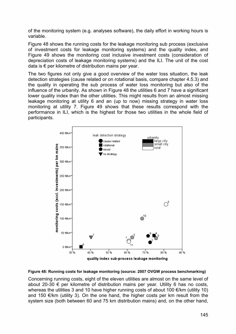
145

of the monitoring system (e.g. analyses software), the daily effort in working hours is variable. Figure 48 shows the running costs for the leakage monitoring sub process (exclusive of investment costs for leakage monitoring systems) and the quality index, and Figure 49 shows the monitoring cost inclusive investment costs (consideration of depreciation costs of leakage monitoring systems) and the ILI. The unit of the cost data is € per kilometre of distribution mains per year. The two figures not only give a good overview of the water loss situation, the leak detection strategies (cause related or on rotational basis, compare chapter 4.5.3) and the quality in operating the sub process of water loss monitoring but also of the influence of the urbanity. As shown in Figure 48 the utilities 6 and 7 have a significant lower quality index than the other utilities. This might results from an almost missing leakage monitoring at utility 6 and an (up to now) missing strategy in water loss monitoring at utility 7. Figure 49 shows that these results correspond with the performance in ILI, which is the highest for those two utilities in the whole field of participants.

Figure 48: Running costs for leakage monitoring (source: 2007 OVGW process benchmarking)

Concerning running costs, eight of the eleven utilities are almost on the same level of about 20-30 € per kilometre of distribution mains per year. Utility 6 has no costs, whereas the utilities 3 and 10 have higher running costs of about 100 €/km (utility 10) and 150 €/km (utility 3). On the one hand, the higher costs per km result from the system size (both between 60 and 75 km distribution mains) and, on the other hand,

146

from a relatively complex water supply system with some system input points, several assets (storage tanks, bulk delivery points etc.), several DMAs and the fact that the monitoring system is not fully completed (utility 3). Some of the utilities use DMAs (utilities 1, 3, 8 and utilities 9, 10 and 11 partly). Utility number 1 probably has the most diligent DMA system of all the participants with more than 60 DMAs and practicable analysis software. The running costs are quite low and the investment costs for this system are not out of range.

Figure 49: Leakage monitoring costs inclusive investment costs for leakage monitoring systems (source: 2007 OVGW process benchmarking)

One of the larger cities (utility 8) uses a mixed strategy (with some DMAs) and has therefore higher costs for leakage monitoring. This can be seen in Figure 49 where the investment costs are considered, and which are higher than those of the other three large cities (utilities 2, 4 and 6). As we can see in Figure 48, the running costs for leakage monitoring are nearly the same for utilities 2, 4 and 8 but the level of leakage is quite different between utility 8 and the other large cities. This difference is probably not just a result of a more advanced leakage monitoring. In fact the leak detection and the infrastructure management also have a large influence.

6.2.4. Leak detection sub process results The main criteria for the sub process of leak detection are the leak detection strategy (cause related or on a rotational basis, compare chapter 4.5.3), the leak detection technology used and the amount of leak detection.

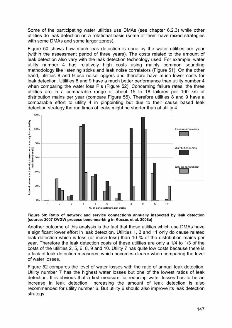
147

Some of the participating water utilities use DMAs (see chapter 6.2.3) while other utilities do leak detection on a rotational basis (some of them have mixed strategies with some DMAs and some larger zones). Figure 50 shows how much leak detection is done by the water utilities per year (within the assessment period of three years). The costs related to the amount of leak detection also vary with the leak detection technology used. For example, water utility number 4 has relatively high costs using mainly common sounding methodology like listening sticks and leak noise correlators (Figure 51). On the other hand, utilities 8 and 9 use noise loggers and therefore have much lower costs for leak detection. Utilities 8 and 9 have a much better performance than utility number 4 when comparing the water loss PIs (Figure 52). Concerning failure rates, the three utilities are in a comparable range of about 15 to 18 failures per 100 km of distribution mains per year (compare Figure 55). Therefore utilities 8 and 9 have a comparable effort to utility 4 in pinpointing but due to their cause based leak detection strategy the run times of leaks might be shorter than at utility 4.

Figure 50: Ratio of network and service connections annually inspected by leak detection (source: 2007 OVGW process benchmarking in KOELBL et al. 2008a)

Another outcome of this analysis is the fact that those utilities which use DMAs have a significant lower effort in leak detection. Utilities 1, 3 and 11 only do cause related leak detection which is less (or much less) than 10 % of the distribution mains per year. Therefore the leak detection costs of these utilities are only a 1/4 to 1/3 of the costs of the utilities 2, 5, 6, 8, 9 and 10. Utility 7 has quite low costs because there is a lack of leak detection measures, which becomes clearer when comparing the level of water losses. Figure 52 compares the level of water losses with the ratio of annual leak detection. Utility number 7 has the highest water losses but one of the lowest ratios of leak detection. It is obvious that a first measure for reducing water losses has to be an increase in leak detection. Increasing the amount of leak detection is also recommended for utility number 6. But utility 6 should also improve its leak detection strategy.

0%

20%

40%

60%

80%

100%

120%

1 2 3 4 5 6 7 8 9 10 11Nr. of participating water works

Ratio

of n

etw

ork

and

serv

ice

conn

ectio

ns a

nnua

lly in

spec

ted

by

leak

det

ectio

n (%

)

P7S212_A nte il m itte lsLeckortungsverfahrenunters uc hterZubringerlei tungen

P7S213_A nte il m itte lsLeckortungsverfahrenunters uc hter Haupt- undVersorgungslei tungen

P7S214_A nte il h insichtl ic hWasserverluste untersuchteHaus anschluss le itungen

transmission mains

distribution mains

service connections

148

Figure 51: Costs of leak detection and ratio of network and service connections annually inspected by leak detection (source: 2007 OVGW process benchmarking)

Figure 52: ILI and proportion of distribution mains annually inspected by leak detection (source: 2007 OVGW process benchmarking)

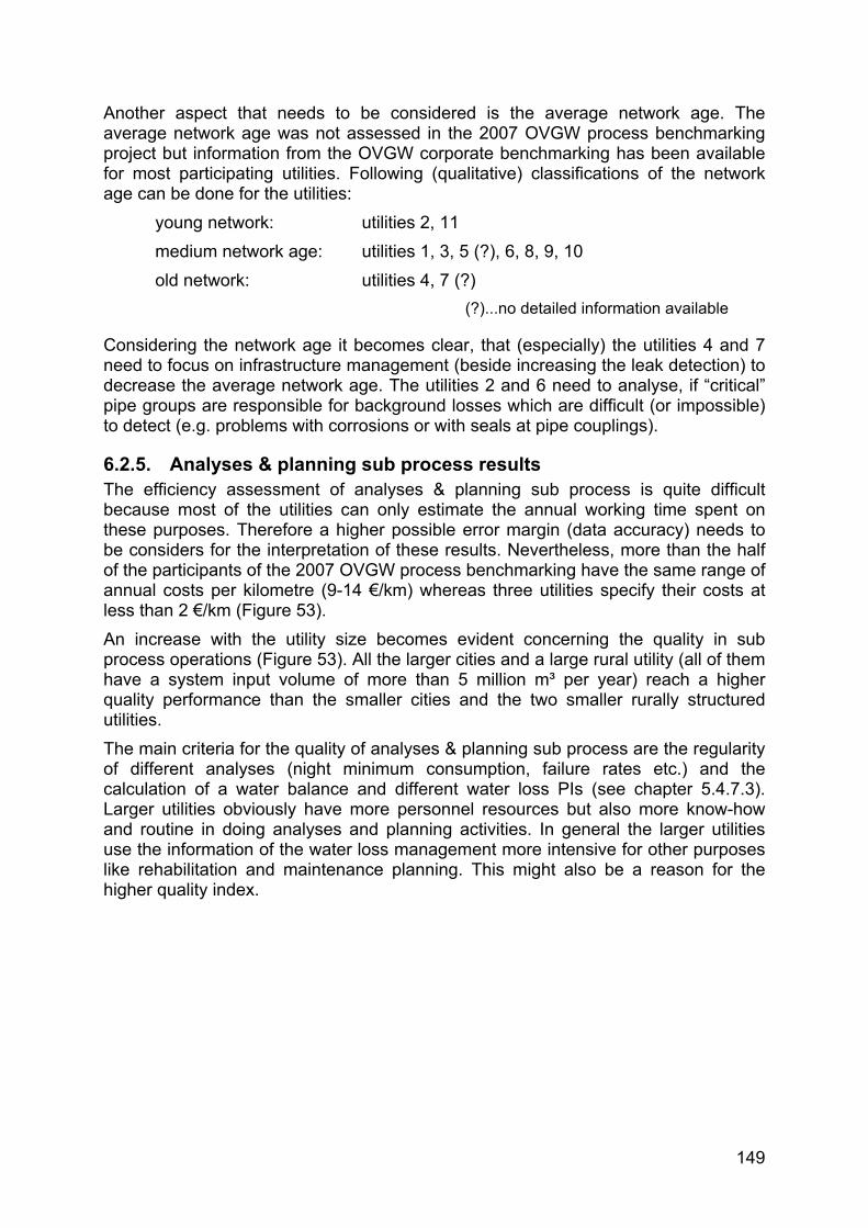
149

Another aspect that needs to be considered is the average network age. The average network age was not assessed in the 2007 OVGW process benchmarking project but information from the OVGW corporate benchmarking has been available for most participating utilities. Following (qualitative) classifications of the network age can be done for the utilities:

young network: utilities 2, 11 medium network age: utilities 1, 3, 5 (?), 6, 8, 9, 10 old network: utilities 4, 7 (?)

(?)...no detailed information available

Considering the network age it becomes clear, that (especially) the utilities 4 and 7 need to focus on infrastructure management (beside increasing the leak detection) to decrease the average network age. The utilities 2 and 6 need to analyse, if “critical” pipe groups are responsible for background losses which are difficult (or impossible) to detect (e.g. problems with corrosions or with seals at pipe couplings).

6.2.5. Analyses & planning sub process results The efficiency assessment of analyses & planning sub process is quite difficult because most of the utilities can only estimate the annual working time spent on these purposes. Therefore a higher possible error margin (data accuracy) needs to be considers for the interpretation of these results. Nevertheless, more than the half of the participants of the 2007 OVGW process benchmarking have the same range of annual costs per kilometre (9-14 €/km) whereas three utilities specify their costs at less than 2 €/km (Figure 53). An increase with the utility size becomes evident concerning the quality in sub process operations (Figure 53). All the larger cities and a large rural utility (all of them have a system input volume of more than 5 million m³ per year) reach a higher quality performance than the smaller cities and the two smaller rurally structured utilities. The main criteria for the quality of analyses & planning sub process are the regularity of different analyses (night minimum consumption, failure rates etc.) and the calculation of a water balance and different water loss PIs (see chapter 5.4.7.3). Larger utilities obviously have more personnel resources but also more know-how and routine in doing analyses and planning activities. In general the larger utilities use the information of the water loss management more intensive for other purposes like rehabilitation and maintenance planning. This might also be a reason for the higher quality index.

150

Figure 53: Costs per km distribution mains for analyses & planning (source: 2007 OVGW process benchmarking)

6.2.6. Leak repair supporting process results Due to its status as a “former” sub process and its special role within infrastructure management, some performance indicators are calculated for the leak repair supporting process.

Figure 54: Average repair costs for leak repair at distribution mains (source: 2007 OVGW process benchmarking)

151

One aspect is the assessment of average repair costs at distribution mains (for failures with leakage). Whereas the rural utilities have average repair costs of less than 2000 € per failure, larger cities have higher repair costs of about 3000 to 3500 € per failure due to the usually more complex situations in larger cities (e.g. pipes of other media e.g. gas; traffic, etc.). Therefore the construction costs are lower in rural regions (note: also the rebuilding of the road surface is in general more expensive in urban situations). Two of the smaller cities lie between these two groups; one of them has higher costs and one of them has costs comparable with rural systems (Figure 54). Another interesting aspect is the correlation of failure rates with the level of water losses. Figure 55 allows a bold interpretation of the situation within the utilities regarding the condition of infrastructure, strategy in leakage monitoring and leak detection and also regarding the effectiveness of water loss management.

Figure 55: Failure rates and ILI (source: 2007 OVGW process benchmarking)

There are four utilities with significantly higher water losses than the other utilities, which have ILIs around 1. The utilities with higher losses are 2, 4, 6 and 7, which use a leak detection strategy on a rotational basis (except utility 2 which uses a mixed strategy) and do not have intensive leakage monitoring. Utility number 7 has high water losses but a very low failure rate. The low failure rate is probably due to a lack of leak detection (compare Figure 52). There may be many undetected leaks within this supply system. A decrease in leakage can be expected with an increase in leak detection. Utilities 2 and 6 have medium failure rates and a medium to high level of water losses. The ratio of mains annually inspected by leak detection of these two utilities is about 20-25 %. Beside an increase in leak detection, optimisations of leakage monitoring and of the leak detection (strategy and technology) are also recommended.

152

Utility number 4 seems to be in a more difficult situation (higher average age of network). Although a lot of leak detection is done and many failures are repaired, the amount of water losses is relatively high. Beside intensive leak detection measures, other infrastructure measures like an effective rehabilitation planning, should also be taken into consideration. All the utilities with lower water losses use a cause based or mixed leak detection strategy. It is evident that intensive leakage monitoring enables short awareness times and, combined with cause based leak detection, the run times of leaks are kept short. Of course, it has to be taken into consideration that most of these systems (except utility number 8) are small cities or rural water supply systems, which makes the situation easier. Nevertheless, the example of utility number 8 shows that it is possible to achieve a good level of leakage even in large and historic cities.

6.2.7. Quality indices results The problems in assessing process quality and calculating quality indices has already been discussed in chapter 5.4.7. Figure 56 shows the quality indices of all the sub and supporting processes and also of the main process (overall process), as calculated in the 2007 OVGW process benchmarking. The results of the quality indices are plausible regarding their performance in water loss management for almost all the utilities. E.g., utility number 6 has high quality indices in leak repair (e.g. good documentation of failures) and in infrastructure management (e.g. good rehabilitation planning) and, on the other hand, a weak performance in leakage monitoring. This corresponds with the results discussed in the previous chapters. There is also good (or quite good) correlation for the utilities 3, 4, 5, 7, 8, 9, 10 and 11. For the utilities 1 and 2 it seems that the quality indices do not reflect their “real” performance in water loss management. Utility number 1 probably has one of the most diligent monitoring systems of all the participants and a quite low level of water losses but attains only an average quality level. Utility 2 has the highest quality index for the main process but has higher water losses than utility 8. Therefore the quality indices were adapted on the basis of these experiences. Following adaptations have been implemented (compare chapter 5.4.7):

• consideration of water losses (ILI)

• adaptation of assessment of qualification of staff

• adaptation of weightings for the main process quality index Figure 57 shows a comparison of the quality index for the qualification of staff calculated within the 2007 OVGW process benchmarking with the adapted index described in chapter 5.4.7. Larger utilities (e.g. utilities 1, 2, 6, 8) especially benefit from this adaptation and reach higher quality indices for this supporting process because it is not the proportion of staff that fulfils various qualification criteria. There is only an evaluation if there is staff with these qualifications (but not the proportion of staff).

153

Figure 56: Summary of quality indices (source: 2007 OVGW process benchmarking)

0%10%

20%

30%

40%

50%

60%

70%

80%

90%

100%

12

34

56

78

910

11

quality index (%)

utili

ty n

umbe

r

P7H

11_Q

ualit

ätsi

ndex

Hau

ptpr

ozes

s

P7S1

11_Q

ualit

ätsi

ndex

SP

1 W

asse

rver

lust

über

wac

hung

P7S2

11_Q

ualit

ätsi

ndex

SP

2 Le

ckor

tung

P7S4

11_Q

ualit

ätsi

ndex

SP

4 An

alys

e &

Pla

nung

P7H

001_

Qua

lität

sind

ex

Hilf

spro

zess

Infr

astr

uktu

r-M

anag

emen

t

P7S3

01_Q

ualit

ätsi

ndex

SP

3 R

epar

atur

von

Sch

äden

P7H

002_

Qua

lität

sind

ex

Hilf

spro

zess

Mita

rbei

terq

ualif

ikat

ion

mai

npr

oces

s

leak

age

mon

itorin

g

leak

dete

ctio

n

anal

yses

& p

lann

ing

infra

stru

ctur

em

anag

emen

t

leak

repa

ir

qual

ifica

tion

ofst

aff

ILI c

lass

ifica

tion:

A B C

154

Figure 57: Comparison of quality indices for qualification of staff

The adaptation of the quality indices also has an influence on the quality index of the main process. Utilities with low water losses benefit from the consideration of the level of water losses whereas utilities with high water losses achieve a lower main process quality index. In Figure 58 the adapted quality index for the main process is compared with the original one. The utilities with low water losses (utilities 1, 3, 5, 8, 9, 10 and 11) now reach a higher level of main process quality, whereas the utilities number 2, 4, 6 and 7 stay almost at the same quality level. Utility 2 reaches a higher quality index of staff but due to the ILI of about 3 the main process quality index does not change.

Figure 58: Comparison of quality indices for main process

0%

20%

40%

60%

80%

100%

1 2 3 4 5 6 7 8 9 10 11

QI q

ualif

icat

ion

of s

taff

utility number

QI qualification of staff (adopted) QI qualification of staff (OVGW 2007)

0%

20%

40%

60%

80%

100%

1 2 3 4 5 6 7 8 9 10 11

QI m

ain

proc

ess

utility number

QI main process (adopted) QI main process (OVGW 2007)

155

6.2.8. Best-practices workshop A one-day best-practices workshop with the objectives of analysing the results of the process comparison and giving an exchange of experiences to derive measures for improvement was the last “official” step in the field test. After an introduction of the most important results of the process comparison, three utilities presented different strategies and technologies in water loss monitoring and leak detection:

• utility number 1: leakage monitoring on the basis of DMAs and cause based leak detection

• utility number 6: leak detection on a rotational basis (no DMAs)

• utility number 9: leak detection with noise loggers The discussion about these different strategies was followed by analyses of the results of single utilities in comparison with the other utilities. The quality matrix was very helpful for this purpose. On the basis of the eleven quality matrixes, which were printed next to each other on large posters (Figure 59), it was very easy to get an overview about the strengths and weaknesses of each utility. The derivation of concrete measures for improvement was also made easier by this matrix.

Figure 59: Analyses of the quality matrix within the best-practice workshop (source: 2007 OVGW process benchmarking)

Concerning leakage monitoring following improvements could have been derived (selected examples):

• increasing of accuracy of system input metering

• implementation of DMAs

• implementation or optimisation of minimum night flow analyses

156

• modernisation of SCADA system (combination with leakage monitoring software)

• implementation of pressure monitoring

• data gathering for first information about leak location For the sub process of leak detection following optimisation potentials could have been identified (selected examples):

• change of leak detection strategy (e.g. cause based instead of leak detection on rotational basis)

• optimisation of the location time

• documentation of leak detection activities (where, when, what methodology)

• use of temporary noise loggers Following examples of improvement potentials in analyses & planning have been identified:

• failure statistics for single zones and for single pipe groups

• internal analyses of efficiency in water loss management (cost – benefit analyses)

• extended publication of water loss performance indicators (several PIs) in annual reports

• improvement of accuracy of unbilled consumption and other water balance input data

Frequently mentioned improvement potentials for the infrastructure management are for example:

• adaptation of inspection intervals (according OeNORM B 2539 - OVGW W 59)

• hydraulic modelling

• optimisation of rehabilitation planning (on basis of failure rates)

• decrease of maximum service pressure (in some cases)

• failure documentation

• optimisation of repair times Some of the utilities might have potential for increasing staff qualification in water loss management. For the improvement of the qualification of staff e.g. the OVGW offers training courses on leak detection. Finally experiences about the following topics were exchanged in detailed discussions:

• different aspects of flow metering and customer meter reading

• zone measurements in large networks (permanent and temporary)

• advantages and disadvantages of different leak detection technologies

157

• H2-tracer gas technology

• use of measuring vehicles

• leak detection at plastic pipes

• pressure monitoring The feedback of the utilities to the workshop was very positive and all of them said they had benefitted from the process benchmarking project and, in particular, the best-practices workshop. As an outcome of the project, and on basis of the workshop results, the utilities can optimise their water loss management. Some utilities expressed the wish to change their water loss management strategy due to the experiences from this project.

6.3. Methodical experiences of the field test The most important outcome of the field test from the 2007 OVGW process benchmarking is that the process benchmarking system developed for the process of physical water loss management works. Following the feedback of the eleven participating water supply utilities, the field test was more than just a test run. In fact the utilities already had a useful outcome of the project. The process benchmarking system fulfilled most of the requirements for such an instrument and, therefore, the benefit for the utilities was satisfactory. But, of course, the field test also provided important information about optimisation potentials of the process benchmarking system itself and was therefore essential for the quality of the process benchmarking system described in this PhD thesis. Concerning data availability, it was found that most of data can be provided from the utilities with an adequate effort, even if some data need to be estimated. Some utilities had problems submitting accurate data about the working hours for several process steps. Therefore it makes sense to implement (or adapt existing) work time documentation systems within the utilities to gather more detailed information about the effort in work time. Concerning cost allocation, adaptations of documentation system within the utilities are useful for making future comparisons and utility internal management easier. An important adaptation within the process structure was the change of leak repair from a sub process to a supporting process (compare chapter 5.2). The structure of variables and also the structure of performance indicators changed essentially due to this modification. Regarding comparability, it was found that a comparison at the level of sub processes or even at the level of single tasks works well, whereas a performance comparison of the main process of physical water loss management is difficult. Therefore it is very important to consider the frame conditions of the participating companies. The condition of the infrastructure is very important (age of pipes, level of water losses) but also the general network instrumentation. The average age of the pipe network was not assessed in the 2007 process benchmarking project but this information is essential for the interpretation of water loss management data and should therefore be assessed in future projects (as context information).

158

On the basis of the results from the single sub processes the question what is the right strategy in leakage monitoring and leak detection can be answered. Under consideration of the frame conditions it is possible to reveal the advantages and disadvantages of each strategy in a qualitative but also from an economic point of view. For better comparability of leakage monitoring costs and the total costs of the main process it is necessary to consider the investment costs of leakage monitoring systems (e.g. measurement equipment, SCADA systems). The experience in allocating these costs showed that it is difficult to estimate the portion of investment costs which is related to leakage monitoring. The problem is that these systems are not only used for leakage monitoring in general but also for controlling the water supply system (e.g. control of pumps). In chapter 6.2 the influence of investment costs for leakage monitoring systems was discussed on the basis of the results for the main process and the leakage monitoring sub process. The comparability of highly aggregated quality indices must be valued critically. The quality index for staff qualifications had to be overworked, because larger utilities were disadvantaged due to the consideration of the proportion of staff qualified for different tasks (see chapter 5.4.7 and 6.2.7). The consideration of the level of water losses was implemented for the quality index of the main process. These measures lead to a better comparability of quality indices. The need for some minor modifications of definitions like the change of the status of a variable to context information (e.g. “ci201a, leak detection during meter reading”) is not discussed here. The implementation of additional verbal descriptions as a complement to the “hard facts” in form of variables and performance indicators seems to be important from a methodical point of view. These verbal descriptions about the process operation of single sub and supporting processes should provide useful information for two aspects: to enable a better illustration of the process operation and to identify common practises which should be implemented into the process benchmarking system (compare chapter 5.6). The experience with the quality matrix was very positive. Together with the performance indicators, the structured quality matrix enables a good overview of the strengths and weaknesses in process operation and it is easily possible to derive measures for improvement. Another very positive experience of the field test was the best-practices workshop in which the results were discussed in detail and the utilities had the opportunity to exchange their experiences. Experiences with the OVGW project show that one single workshop day is a good start for exchanging experience. However, due to the many aspects which have to be considered in water loss management, further workshops and/or discussions and analyses, maybe in smaller groups or even bilaterally between two utilities are useful and sometimes necessary to derive concrete measures for improvement and to reach the aim of benchmarking: learning from each other.

159

7. Summary and conclusions The objective of this PhD thesis was to create a process benchmarking system for the process of physical water loss management. Aspects of managing non-revenue water (NRW) were not part of this thesis. The process benchmarking system developed is based on recent developments in performance assessment and covers aspects of modern water loss management. The process benchmarking system enables an assessment of the performance of water supply utilities in physical water loss management from an economic point of view as well as from technical quality aspects. The system meets the demands made on performance assessment tools (compare chapter 1.2).

• In the course of a mapping the process the process of physical water loss management a diligent, clear process structure was worked out. The process structure is easy to understand and all parts of the process (sub processes, supporting processes) are described in detail. Due to the hierarchical structure the performance assessment can be done for different process levels: for the main process as well as for sub processes or even single tasks.

• The process benchmarking system has been developed on the basis of recent developments in water loss management and benchmarking. Beside information from publications of the IWA Water Loss Task Force and many personnel discussions with international experts in the field of water loss management, the latest developments in benchmarking were also considered. Experts from the Austrian water supply utilities were also involved in the system development. The merging of latest scientific developments with practical experiences guaranties an up-to-date system with a good practical applicability.

• The objective of simple data gathering was perhaps not fully fulfilled. Endeavours were made to work out a simple cost allocation system. However, because, in general, the cost data needed are not directly available from common cost documentations within the utilities, more effort in data collection is necessary. The query of context-information happens with selective lists, which keeps the effort as low as possible. The average time for data collection in the field test was about 3 person-days per utility, which can be seen as an arguable expenditure of time.

• A central point in data comparisons is the consideration of data quality. Therefore the accuracy and reliability was considered for all the variables and all performance indicators were indicated by a possible error margin (expressed in percentages or by a data quality classification from A-D, see chapter 5.3.1).

• Another important objective was to create a transparent process benchmarking system without using “black-box” solutions. Most of the performance indicators are quite simple, e.g., costs per kilometre or working hours per 100 service connections. It is more difficult to give full transparency with the highly aggregated quality indices. The calculation of the quality indices with all its weightings is described in detail within these PhD thesis but it is difficult to provide that information in a “user friendly” way. Nevertheless, it

160

is possible to understand the criteria behind the indices in combination with the quality matrix.

• The system developed is applicable for all structures and all sizes of water supply systems for direct supply – rural, urban and metropolitan structures. An application of this process benchmarking system for bulk supply systems is not foreseen. Therefore, adaptations would be necessary due to other demands in water loss management of bulk supply systems than in those systems with a direct supply to customers.

• Of course it is necessary to consider the different structural parameters of different water supply systems in the performance comparison and data interpretation. Therefore a lot of context information is necessary and various grouping criteria and explanatory factors need to be defined (e.g., urbanity or the strategy in leak detection). A meaningful performance comparison is only possible in “comparable” groups” (clusters) of similarly structured utilities.

• Concerning the demand of creating a voluntary and anonymous system, the experiences of the field test show that it makes sense to use synonyms (e.g. numbers or letters) in data illustration to preserve anonymity (especially for publications), but when exchanging experiences within the workshops all utilities were of the opinion that it makes sense to abolish the restriction of anonymity within the field of participants. Voluntary participation is a must for process benchmarking as it is a fundamental idea of benchmarking in general. It is not possible to attain success by forcing utilities to participate in process benchmarking. Therefore this instrument is not appropriate for regulating water utilities. Other instruments (e.g. yardstick-competitions) are necessary for this purpose (compare chapter 2.6.3).

• The system stood a field test in the Austrian water supply sector. Eleven water supply utilities of different sizes and relevant structures (rural, small city, large city) participated in this first project run. The field test was essential for the quality of the process benchmarking system because the field test provided important information about optimisation potentials of the process benchmarking system itself. Nevertheless, the process benchmarking system already fulfilled most of the requirements during the field test and therefore the utilities were satisfied with the benefits they gained.

The process benchmarking system for physical water loss management has many benefits for water supply utilities and can be used for several purposes:

• finding a strategy

• finding a methodology

• improvement in efficiency

• improvement in quality of process operation

• modernisation The main process results can be helpful for the purpose of finding the right strategy in water loss management. General aspects of economic performance, but also the level of water losses can vary between different strategies. The system enables to

161

determine whether the strategy used in water loss management is effective or not. If not, the system provides decision support to find the best strategy for a utility. E.g., one outcome of the field test is the fact that utilities with a strong focus on leakage monitoring in general achieve a lower level of water losses than utilities without leakage monitoring. The total costs in water loss management of utilities with focus on monitoring are not higher because the effort in leak detection is usually much lower than with leak detection only on a rotational basis. Another aspect is the use of the process benchmarking system as a decision support system for an optimal mix of methodologies in leakage monitoring (e.g., functions of SCADA systems) and technical equipment for leak detection (e.g., cost and benefit of noise loggers). Of course the system supports an improvement in efficiency and quality of process operation. The system should show where there is room for improvements within the process operation. This means detecting inefficiencies but also identifying potentials for technical (qualitative) optimisations. The methodologies of corporate benchmarking and process benchmarking, and hence also the process benchmarking system for physical water loss management, are instruments which support modernisation and an increase of efficiency in the water supply sector, which is an important objective of the European Commission and the European Parliament. Beside the practical applicability, this PhD thesis provides some interesting input for scientific progress in the field of performance assessment in the water supply sector. The PhD thesis can be seen as a further developmental step in the methodology of benchmarking at process level. Whereas many process benchmarking activities are based on almost qualitative process comparisons, this thesis describes the approach of a structured process analyses. Comprehensible performance comparisons are made possible due to the use of “metric” elements in process benchmarking in the form of a hierarchical process structure with performance indicators according to this structure. This is the basis for a process benchmarking with larger groups of participants. It opens the possibility for gathering a larger quantity of process performance data which are the basis for the definition of significant benchmarks. The use of “metric” elements in process benchmarking leads to a discussion of the definition of process benchmarking. Up to now the IWA terminology has distinguished between “metric” and “process” benchmarking, whereas in Germany the term “corporate” instead of “metric” has been used in recent publications. The approach of this process benchmarking systems is a further argument that supports the term “corporate” instead of “metric” benchmarking. In addition to these general aspects regarding the methodology of benchmarking, this work represents an innovation concerning a process analysis of physical water loss management on a quantitative basis. Whereas other process benchmarking projects of water loss management (e.g. Canada or the Scandinavian Six-Cities Group project) have used a qualitative approach up to now, the approach developed in this thesis is based on a structured process mapping that enables quantitative process comparisons of the process of physical water loss management.

162

A further innovation is the quality matrix developed for the assessment of the quality in process operation and for the derivation of concrete measures for improvement. The matrix includes about 100 single criteria of the three sub processes and the supporting processes and was a central element for the exchange of experiences in the best-practices workshop. The function of the system as a decision support system for the physical water loss management has already been discussed above, but this aspect also seems to be important from the scientific point of view.

8. Outlook on future research As an outlook on future research, an enlargement of the process benchmarking system from physical water loss management to non-revenue water management can be foreseen. In 2007 the IWA Water Loss Task Force, under the leadership of Roland Liemberger, started an initiative on mapping the process of non-revenue water management. The aim of this initiative is the development of a standardised process structure as a basis for future international process comparisons and benchmarking activities. An intermediate result of this work was presented at the IWA World Water Congress 2008 in Vienna (KOELBL et al. 2008c). For an international use (especially in developing countries) of this process benchmarking system an enlargement of the system for the methodology of pressure management will be necessary. This aspect was not considered in the Austrian OVGW process benchmarking system because the classical pressure management methodologies are not practiced in Austria (compare chapter 4.6). Another aspect that could be interesting to implement is the analysis of the economic level of leakage (e.g. LAMBERT & FANTOZZI 2005), which was also not considered in this work. The economic level of leakage is reached, when further water loss reductions are uneconomical. Due to the fast development of new leak detection and leakage monitoring equipment it will be necessary to adapt the existing process benchmarking system after a certain time. In parallel with the generation of this PhD thesis the Austrian Association for Gas and Water (OVGW) has revised the OVGW W 63 (1993) guideline which deals with water losses in water distribution systems. Parts of this thesis were incorporated into the new OVGW W 63 (in press) like descriptions of performance indicators, the classification scheme for real losses per connection per day and a description of leak detection methodologies. As a final comment there should be a reminder that the successful operation of process benchmarking projects at a high quality level requires a qualified and experienced project team and, in particular, motivated participants. I hope that this work gives support in the battle against water losses and will help many water utilities to improve their water loss management.

163

References ACHTIENRIBBE, G.E. (1997): Die Trinkwasserversorgung in den Niederlanden –

strukturelle Veränderungen. – gwf Wasser Abwasser 138. Jg., Nr. 11, p. 548-550, Germany.

ALEGRE, H, HIRNER, W, BAPTISTA, J. M. AND PARENA, R (2000): Performance indicators for water supply services. - IWA Manual of Best Practice, IWA Publishing, London, UK. ISBN: 1900222272.

ALEGRE, H., BAPTISTA, J.M., CABRERA, E., CUBILLO, F., DUARTE, P., HIRNER, W., MERKEL, W. & R. PARENA (2006): Performance Indicators for Water Supply Services. - Second Edition, Manual of Best Practice, IWA Publishing, London, UK. ISBN 1843390515.

AWWA (2003): AWWA Water Loss Control Committee Report. - AWWA Journal, 98/8, Denver, USA.

BROTHERS, K. (2002): DMA Design & Application for Non-Revenue Water Reduction in Canada. - IWA Conference “Leakage Management – A Practical Approach”, Conference Proceedings, Cyprus.

CAMP, R. (1989): Benchmarking: The Search for Best Practices that Lead to Superior Performance, ASQC Quality Press, Milwaukee, USA.

CHARALAMBOUS, B. (2008): Bridging the water crisis gap: the role of water loss management. – Water21, October 2008, IWA Publishing, London, UK. ISSN 1561-9508.

CLAUSEN, H. & U. SCHEELE (2001): Benchmarking und Yardstick Competition – Ansätze vergleichenden Wettbewerbs in der Wasserwirtschaft. - Wirtschaftswissenschaftlicher Diskussionsbeitrag V-232-01, Institut für Volkswirtschaftslehre I, Carl von Ossietzky Universität Oldenburg.

COST (2008): www.cost.esf.org, 24th of October 2008. COST C18 (2008): www.costc18.org, 24th of October 2008. DICKINSON, M. A. (2008): How important is structured training in achieving maximum

benefits? Is it overlooked by utilities and is there a need for further development in a continuously changing environment? - Presentation at IWA World Water Congress 2008. Vienna, Austria.

DIJKGRAAF, E., DE JONG, R., VAN DE MORTEL & others (1997): Moeglijkheden tot Marktwerking in de Nederlandse watersector. – Study in order of Ministry of Economic Affairs. Ocfeb Erasmus Universiteit Rotterdam, Netherlands.

DVGW - Guideline W 392 (2003): Network inspection and water losses – activities, procedures and assessment. – DVGW, Bonn, Germany.

DWA-Regelwerk Merkblatt DWA-M 149-4 (Draft Version from November 2007): Zustandserfassung und –beurteilung von Entwässerungssystemen außerhalb von Gebäuden; Teil 4: Detektion von Lagerungsdefekten und Hohlräumen in der Umgebung erdverlegter Leitungen. – DWA, Hennef, Germany.

EUROPEAN COMMISSION (2003): Green Paper on services of general interest. COM (2003) 270. – Brussels, Luxemburg.

164

EUROPEAN COUNCIL (1998): Directive 98/83/EC of 3 November 1998 on the quality of water intended for human consumption. - Official Journal of the European Communities, Brussels, Belgium.

EUROPEAN PARLIAMENT (2000): Directive 2000/60/EC of the European Parliament and of the Council of 23rd of October 2000 establishing a framework for Community action in the field of water policy, Luxembourg.

EUROPEAN PARLIAMENT (2003): Resolution of the European Parliament on the Green Paper on services of general interest. Plenary session document A5-0484/2003 to COM (2003) 270 – (2003/2152(INI)), Strasbourg, Luxemburg.

FARLEY, M. & S. TROW (2003): Losses in Water Distribution Networks – A Practitioner’s Guide to Assessment, Monitoring and Control. – IWA Publishing, London. ISBN 1900222116.

FARLEY, M. (2007): Finding the “difficult” leaks. – Water 21, December 2007, IWA Publishing, London, UK. ISSN 1561-9508.

GANGL, G. & J. KOELBL (2009): Anwendbarkeit des Infrastructure Leakage Index - ILI für kleinere Versorger und Messzonen (DMAs). – gwf Wasser Abwasser 150. Jg., Heft 4/2009, Germany.

GIRSBERGER W. (2003): HACCP – Hazard Analysis and Critical Control Points in Modern Management Systems of Water Suppliers. – SVGW Swiss Association for Gas and Water, Switzerland.

HEIN, A., LÉVAI, P. & W. MERKEL (2008): Process Indicators for drinking water production – a unified approach and its pilot application in Germany. - Performance Assessment of Urban Infrastructure Services. IWA Publishing, London, UK. ISBN 978-18-433-9191-3.

HIRNER, W. & W. MERKEL (2002): Benchmarking als Mittel des organisierten Wettbewerbs. – 26. Wassertechnisches Seminar. Berichte aus Wassergüte- und Abfallwirtschaft, Nr.173/2002, S.1-30, TU München, Germany.

HORVATH, P. & N.R. HERTER (1992): Benchmarking: Vergleich mit den Besten der Besten (Benchmarking: comparison with the best of the best). - Controlling, Vol. 4 No. 1, January-February, pp. 4-11.

ISO 24510 (2007): Activities relating to drinking water and wastewater – Guidelines for the improvement and for assessment of the services to users. – International Organisation for Standardisation, Geneva, Switzerland.

ISO 24511 (2007): Activities relating to drinking water and wastewater – Guidelines for the management of wastewater utilities and for the assessment of wastewater services. – International Organisation for Standardisation, Geneva, Switzerland.

ISO 24512 (2007): Activities relating to drinking water and wastewater – Guidelines for the management of drinking water utilities and for the assessment of drinking water services. – International Organisation for Standardisation, Geneva, Switzerland.

IWA (2008): www.iwahq.org, 24th of October 2008. IWA/WSAA (2006): Background to the IWA/WSAA process benchmarking project. –

Information provided by IWA/WSAA process benchmarking. London, UK.

165

KIESL H. & J. SCHIELEIN (2002): Effizienz- und Qualitätsuntersuchung der kommunalen Wasserversorgung in Bayern (EffWB), Final Report for year 2000. Rödl & Partner, Nuremberg, Germany.

KIESL H. & J. SCHIELEIN (2005): Effizienz- und Qualitätsuntersuchung der kommunalen Wasserversorgung in Bayern (EffWB) 2004. – Final Public Report on Bavarian project 2004/05). Rödl & Partner, Nuremberg, Germany.

KIESL H. (2008): Effizienz- und Qualitätsuntersuchung der kommunalen Wasserversorgung in Bayern (EffWB) 2007. – Final Public Report on Bavarian project 2007). Rödl & Partner, Nuremberg, Germany.

KINGDOM B., LIEMBERGER R. & P. MARIN (2006): The Challenge of Reducing Non-Revenue Water (NRW) in Developing Countries - How the Private Sector Can Help: A Look at Performance-Based Service Contracting. - Water Supply and Sanitation Sector Board Discussion Paper Series No. 8, The World Bank, Washington, DC, USA.

KLEIN, D., PETERSOHN, D. & B. PAETSCH (2008): Benchmarking Laboratory Processes for Drinking-Water Quality Monitoring. - Performance Assessment of Urban Infrastructure Services. IWA Publishing, London, UK. ISBN 978-18-433-9191-3.

KOELBL, J., LIEMBERGER, R., ROGERS, D., THEURETZBACHER-FRITZ, H., NEUNTEUFEL, R., MAYR, E. & R. PERFLER (2008c): Process Mapping of Non-Revenue Water Management. - Poster at IWA World Water Congress 2008, Vienna, Austria.

KOELBL, J., MARTINEK, D., MARTINEK, P., WALLINGER, CH., FUCHS-HANUSCH, D., ZANGL, H. & A. FUCHS (submitted): Multiparameter Measurements for Network Monitoring and Leak Localising. – Paper submitted for IWA conference Water Loss 2009, Cape Town, South Africa in April 2009.

KOELBL, J., MAYR, E., THEURETZBACHER-FRITZ, H., NEUNTEUFEL, R. & R. PERFLER (2008a): Austrian Case Study on Process Benchmarking of Water Loss Management. - Conference Proceedings Water Loss Management, Telemetry and SCADA in Water Distribution Systems, Ohrid, Macedonia.

KOELBL, J., NEUNTEUFEL, R., THEURETZBACHER-FRITZ, H. & R. PERFLER (2007a): Benchmarking in Österreich – Leistungsverbesserung durch Prozess-Benchmarking. – OVGW Symposium 2007, Conference Proceedings. OVGW, Vienna, Austria.

KOELBL, J., THEURETZBACHER-FRITZ, H., NEUNTEUFEL, R., MAYR, E. & R. PERFLER (2008b): Benchmarking the Processes of Customer Meter Reading and Customer Meter Replacement. – Performance Assessment of Urban Infrastructure Services. IWA Publishing, London, UK. ISBN 978-18-433-9191-3.

KOELBL, J., THEURETZBACHER-FRITZ, H., NEUNTEUFEL, R., PERFLER, R. & R. KRENDELSBERGER (2006): Benchmarking in the Austrian Water Supply Sector: Objectives, Development, Structure and First Results of the 2004 Project. - Water and Environmental Management Series, 12, 197-204, London, UK. ISBN 1843395134.

KOELBL, J., THEURETZBACHER-FRITZ, H., NEUNTEUFEL, R., PERFLER, R., GANGL, G., KAINZ, H. & R. HABERL (2007b): Experiences with Water Loss PIs in the Austrian Benchmarking Project. - Proceedings Water Loss 2007 Volume I, Bucharest, Romania. ISBN 978-973-7681-25-6.

166

KOUZMIN, A., LOEFFLER, E., KLAGES, H. & N. KORAC-KAKABADSE (1999): Benchmarking and performance measurement in public sectors - Towards learning for agency effectiveness. - The International Journal of Public Sector Management, Vol. 12 No. 2, 1999, pp. 121-144. MCB University Press, UK.

LAMBERT, A. & R. D. MCKENZIE (2002): Practical Experience in using the Infrastructure Leakage Index. - IWA Conference “Leakage Management – A Practical Approach”, Conference Proceedings, Cyprus.

LAMBERT, A. & W. HIRNER (2000): Losses from water supply systems: Standard terminology and recommended performance measures. IWA Blue Pages, London.

LAMBERT, A. (2001): What do we know about pressure:leakage relationships?. - Proceedings IWA Conference “System Approach to Leakage Control and Water Distribution Systems Management”, Brno, Czech Republic. ISBN 80-7204-197-5.

LAMBERT, A. (2002): International Report on Water Loss Management and Techniques. – Water Science and Technology: Water Supply, 2(4) (2002), 1-20, London, UK.

LAMBERT, A. (in press): Ten Years Experience in using the UARL Formula to calculate Infrastructure Leakage Index. – IWA Water Loss 2009 Conference Proceedings, Cape Town, South Africa in April 2009.

LAMBERT, A., BROWN, T.G., TAKIZAWA, M. & D. WEIMER (1999): A Review of Performance Indicators for Real Losses from Water Supply Systems. AQUA, Vol. 48 No 6. ISSN 0003-7214.

LAMBERT, A. & M. FANTOZZI (2005): Recent advances in calculating economic intervention frequency for active leakgage control, and implications for calculation of economic leakage levels. – IWA Conference on Water Economics, Statistics, and Finance, Conference Proccedings, Rethymno, Greece.

LARSSON, M., PARENA, R., SMEETS, E. & I. TROQUET (2002): Process benchmarking in the water industry. - IWA Manual of Best Practice, IWA-Publishing, London, UK. ISBN 1-84339-010-8.

LIEMBERGER, R. & R. MCKENZIE (2005): Accuracy Limitations of the ILI - Is it an Appropriate Indicator for Developing Countries?. - IWA Leakage 2005, Conference Proceedings, Halifax, Canada.

LIEMBERGER, R. (2005): The new German water loss regulations in context with other international applications of the IWA water balance and real loss performance indicators. – Conference Proceedings IWA Conference Efficient 2005, Santiago de Chile, Chile.

LIEMBERGER, R. (2006): Das neue IWA-System zur Beurteilung von Wasserverlusten. - Proceedings Symposium Wasserversorgung 2006, OVGW, Vienna, Austria.

LIEMBERGER, R. (2007): Foreword of Conference Proceedings.- Proceedings Water Loss 2007 Volume I, Bucharest, Romania. ISBN 978-973-7681-25-6.

LIEMBERGER, R., BROTHERS, K., LAMBERT, A., MCKENZIE, R., RIZZO, A. & T. WALDRON (2007): Water Loss Performance Indicators.- Proceedings Water Loss 2007 Volume I, Bucharest, Romania. ISBN 978-973-7681-25-6.

LMSVG (BGBL 13/2006): Lebensmittelsicherheits- und Verbraucherschutzgesetz. – Austrian law, Austria.

167

MAIN, D. (2008a): How to Use 10 Years of Benchmarking Data to Guide Performance Improvement. – Presentation at IWA Conference PI08 – Performance Assessment of Urban Infrastructure Services, Valencia, Spain.

MAIN, D. (2008b): Personal information to the Canadian benchmarking project. May and June 2008. Canada.

MAIN, D., NG, L. & A NORTH (2008): The Canadian national water and wastewater benchmarking initiative: Using process to drive improvement. Strategic Management of Water in Urban Areas. – Performance Assessment of Urban Infrastructure Services. IWA Publishing, London, UK. ISBN 978-18-433-9191-3.

MCCORMACK, CH. (2005): Canadian Utilities Learn to Fly through Benchmarking of Water Loss Management. - IWA Leakage 2005, Conference Proceedings, Halifax, Canada.

MCKENZIE, R. S., WEGELIN, W., MOHAJANE, P. & S. SHABALALA (2007): Hidden benefits of smale scale performance based public private partnerships. – Proceedings Water Loss 2007 Volume III, Bucharest, Romania. ISBN: 978-973-7681-27-0.

MERKEL, W. (2001): Performance assessment in the water industry. IWA International Report “Kennzahlen und Benchmarking”, 2. IWA World Water Congress, Berlin, Germany.

MORRISON, J., TOOMS, S. & D. ROGERS (2007): District Metered Areas Guidance Notes. – Guideline of IWA Water Loss Task Force (free available at www.iwaom.org/wltf/).

NAGY, M., LENZ, K., WINDHOFER, G., FÜRST, J. & B. FRIBOURG-BLANC (2007): Data Collection Manual for the OECD/Eurostat Joint Questionnaire on Inland Waters Tables 1-7 - Concepts, definitions, current practices, evaluations and recommendations. –Eurostat, European Commission.

NEBC (2007): The North European Benchmarking Model. Version 1.2, North European Benchmarking Co-Operation, C/o Vewin, The Netherlands.

NEUNTEUFEL, R., PERFLER, R., THEURETZBACHER-FRITZ, H. & J. KOELBL (2007): Explanatory Factor “Average Network Age Index” (NAX) for Mains Failures and Water Losses. Conference Proceedings of LESAM 2007, 2nd Leading Edge Conference on Strategic Asset Management, Lisbon, Portugal.

NEUNTEUFEL, R., THEURETZBACHER-FRITZ, H., TEIX, P., KOELBL, J. & R. PERFLER (2004): Benchmarking und Best Practices in der österreichischen Wasserversorgung – Stufe A. Final Report of OVGW pilot project 2003/04, OVGW, Vienna, Austria.

OeNorm B 2538 (2002): Transport-, Versorgungs- und Anschlussleitungen von Wasserversorgungsanlagen – Ergänzende Bestimmungen zu ÖNORM EN 805 (engl.: Long-distance, district and supply pipelines of water supply systems – Additional specifications concerning ÖNORM EN 805). - Austrian standard, Österreichisches Normungsinstitut, Vienna, Austria.

OeNorm B 2539 – OVGW W 59 (2005): Technische Überwachung von Trinkwasser-versorgungsanlagen. – Austrian standard for technical inspection of water supply systems, Österreichisches Normungsinstitut, Vienna, Austria.

168

OTTILINGER, F. (2004): EffWB-Untersuchung – Nutzen der Untersuchung für die interne Kosten-/Leistungsrechnung und Steuerung. – Conference Proceedings Benchmarking Fachsymposium Effizienz- und Qualitätsuntersuchung der Kommunalen Wasserversorgung in Bayern (EffWB), Nuremberg, Germany.

OVERATH, H. & W. MERKEL (2004): Kennzahlen für die Wasserversorgung: Feldtest des Kennzahlensystems der IWA – Nationales Teilprojekt Deutschland. IWW-Rheinisch-Westfälisches Institut für Wasserforschung GmbH, Mühlheim an der Ruhr.

OVGW W 63 (1993): Wasserverluste in Versorgungsnetzen, Anschlussleitungen und Verbrauchsleitungen – Feststellungen, Beurteilungen und Maßnahmen zur Verminderung. – OVGW directive, OVGW, Vienna, Austria.

OVGW W 63 (in progress): Water Losses in Water Supply Systems. – Update of OVGW directive W 63 (1993), OVGW, Vienna, Austria.

OVGW W 85 (2007): Operation manual for water supply companies. - OVGW directive, OVGW, Vienna, Austria.

OVGW W 100 (2007): Water Supply Pipelines – Operation and Service. – OVGW directive, OVGW, Vienna, Austria.

PICCININ C. (2006): From metric benchmarking to process benchmarking. – Presentation on IWA Conference “Benchmarking Water Supply, Waste Management and Water Control” in Amsterdam, Netherlands.

PILCHER, R. (2007): Leak Location and Repair Guidance Notes and…. The Never Ending War against Leakage. - Proceedings Water Loss 2007 Volume II, Bucharest, Romania. ISBN: 978-973-7681-26-3.

PILCHER, R., HAMILTON, S., CHAPMAN, H., FIELD, D., RISTOVSKI, B. & S. STAPELY (2007): Leak Location and Repair Guidance Notes. – Guideline of IWA Water Loss Task Force (free available at www.iwaom.org/wltf/).

PROFILE OF THE GERMAN WATER INDUSTRY (2008). – published by ATT (Association of Drinking Water from Reservoirs), BDEW (German Association of Energy and Water Industries), DBVW (German Alliance of Water Management Associations), DVGW (German Technical and Scientific Association for Gas and Water), DWA (German Association for Water, Wastewater and Waste), VKU (Association of Local Utilities). wvgw Wirtschafts- und Verlagsgesellschaft Gas und Wasser mbH, Bonn, Germany.

SAX, CH. & M. SCHREITMÜLLER (2007): Monitoring System for the close meshed Water-pipe network to the City of CRAILSHEIM - Germany. – Poster at IWA Specialists Conference Water Loss 2007, Bucharest, Romania.

SIEBERT, G. & S. KEMPF (1998): Benchmarking: Leitfaden für die Praxis. Carl Hanser Verlag Munich Vienna. ISBN 3-446-19342-1.

STAHRE P. & J. ADAMSON (2002): Performance benchmarking – a powerful management tool for water and wastewater utilities.- Watermarque 3 (5) [Online-Journal]. <http://www.pbngroup.com/members_area/3.5/3.5-6cities.pdf> on 26nd of November 2003.

STAHRE P. & J. ADAMSON (2005): Performance assessment as a management tool - Experiences from the Scandinavian Six-Cities Group. – Presentation at COST Action C18 Meeting in February 2005, Catania, Italy.

169

THEURETZBACHER –FRITZ, H., KOELBL, J., KAINZ, H., NEUNTEUFEL, R., PERFLER, R. & R. HABERL (2007): New PI`s and explanatory index factors in the austrian water supply benchmarking system. - EFFICIENT 2007 - The 4th IWA Specialist Conference on Efficient Use and Management of Urban Water Supply, Jeju, Korea.

THEURETZBACHER-FRITZ H. & J. KOELBL (2003). Benchmarking und Best Practices in der österreichischen Wasserversorgung – Methodische Überlegungen zum laufenden Forschungsprojekt. - Schriftenreihe zur Wasserwirtschaft, 41, 241-248, Graz University of Technology, Austria.

THEURETZBACHER-FRITZ, H., NEUNTEUFEL, R., KOELBL, J., PERFLER, R. & E. MAYR (2008): The Right Choice of Denominators and Grouping Factors in Water Supply Metric Benchmarking. – Performance Assessment of Urban Infrastructure Services. IWA Publishing, London, UK. ISBN 978-18-433-9191-3.

THEURETZBACHER-FRITZ, H., NEUNTEUFEL, R., KOELBL, J., PERFLER, R., UNTERWAINIG, M. & R. KRENDELSBERGER (2006): Benchmarking und Best Practices in der österreichischen Wasserversorgung – Stufe B. – Final Report of OVGW project 2005/06, Graz-Wien-Wiener Neustadt, Austria.

THEURETZBACHER-FRITZ, H.,SCHIELEIN, J., KIESL, H., KOELBL, J., NEUNTEUFEL, R. & R. PERFLER (2005): Trans-National Water Supply Benchmarking: The Cross-Border Co-operation of The Bavarian EffWB Project and The Austrian OVGW Project. - Water Science & Technology: Water Supply 6 (2005), 273-280, London, UK.

THORNTON, J. & A. LAMBERT (2005): Progress in practical prediction of pressure:leakage, pressure:burst frequency and pressure:consumption relationships. – Proceedings IWA Konferenz “Leakage 2005”, Halifax, Canada.

THORNTON, J. & A. LAMBERT (2006): Managing pressures to reduce new breaks. – Water 21, December 2006, IWA Publishing, London, UK. ISSN 1561-9508

TWV (BGBl. II Nr. 304/2001 idgF): 304. Verordnung des Bundesministers für soziale Sicherheit und Generationen über die Qualität von Wasser für den menschlichen Gebrauch (Trinkwasserverordnung – TWV). – Austrian Drinking Water Ordinance, Austria.

VEWIN (2001): Reflections of Performance 2000 – Benchmarking in the Dutch Drinking Water Industry. – VEWIN, Rijswijk, Netherlands.

VEWIN (2004): Reflections of Performance 2003 – Benchmarking in the Dutch Drinking Water Industry. – VEWIN, Rijswijk, Netherlands.

VEWIN (2007): Reflections of Performance 2006 – Benchmarking in the Dutch Drinking Water Industry. – VEWIN, Rijswijk, Netherlands.

WIKIPEDIA (2008): www.wikipedia.org, 14th of November 2008. WRG 1959 (BGBl. Nr. 215/1959 idgF): Wasserrechtsgesetz 1959 - WRG 1959 BGBl

1959/215 (Wv). – Austrian law, Ministry of Agriculture, Forestry, Environment and Water Management and Food, Vienna, Austria.

Web site of OVGW benchmarking project: www.trinkwasserbenchmarking.at

170

Appendix

A1. Data collection system 171 A1.1. Contact details 171 A1.2. Basis data 172 A1.3. Water supply system data 173 A1.4. Water balance data 174 A1.5. Process specific data 180

A1.5.1. Data of leakage monitoring sub process 181 A1.5.2. Data of sub process leak detection 183 A1.5.3. Data for analyses and planning sub process 187 A1.5.4. Data for infrastructure management supporting process 190

A1.5.4.1.1. Data for leak repair supporting process 191 A1.5.5. Data for qualification of staff supporting process 195

171

A1. Data collection system All the elements of the data collection system (except supporting data) are indicated by codes. If the definitions of data elements are the same as those in the IWA-PI system (ALEGRE et al. 2006) the IWA-codes are also described within the squared brackets.

A1.1. Contact details Table 49: Contact details (context information)

context information code

utility contact

data

full company name ci01

street and house number ci02

postal code ci03

city ci04

county ci05

fax number ci06

contact person

last name ci07

first name ci08

sex ci09

(academic) title ci10

telephone number ci11

mobile phone number ci12

email address ci13

proxy person

last name ci14

first name ci15

sex ci16

(academic) title ci17

telephone number ci18

mobile phone number ci19

email address ci20

172

A1.2. Basis data Table 50: Basis data (context information)

undertaking profile

context information code Definition value

geographical scope

ci01 [CI1]

[scope of activity of the organisation as a whole]

[nation state

region local]

type of activity ci02 [CI2]

[scope of activity of the organisation as a whole, beyond the water supply]

water supply only water and waste water

multi-utility

type of asset ownership

ci03 [CI3]

[ownership of the water supply infrastructure]

[public private mixed]

legal form ci04 legal form of the organisation as a whole

municipal utility capital company water association water cooperative

accounting system ci05 accounting system used

within the organisation

double-entry accounting fiscal accounting

cash basis accounting

cost accounting

system ci06

is there an existing cost accounting system within the

organisation

yes no n/a

urbanity ci07 structure of the water distribution system

rural small city large city

[IWA Code], [IWA definition] and [IWA unit]…according to ALEGRE et al. (2006)

Table 51: Basis data (supporting information)

employees

supporting information code definition unit

name or group of employee no code name of single employee or name of group of

employees with the same hourly rate -

hourly rate no code personnel costs per hour for the employee or employee group €/h

portion of overhead costs no code portion of overhead costs within the hourly

rates of employees %

173

A1.3. Water supply system data Table 52: Water supply system data (variables)

water supply system

variable code definition unit

measuring zones v001 number of measuring zones within the supply system (pressure zones and/or DMAs) No.

pressure zones v002 number of pressure zones within the supply system No.

DMAs v003 number of DMAs within the supply system No.

mains length v004 [C8]

[total transmission and distribution mains length (service connections not included)] [km]

service connections

v005 [C24] [total number of service connections] [No.]

maximum service pressure head

v006 [CI17]

[maximum target service pressure at any delivery point of the network]

m [kPa]

average service pressure head

v007 [D34]

[average operating pressure at the delivery points], weighted for service connections

m [kPa]

minimum service pressure head

v008 [CI16]

[minimum target service pressure at any delivery point of the network]

m [kPa]

system input meters v009 total number of system input meters within the

whole water supply system No.

system input meters (PCS) v010

total number of system input meters within the whole water supply system which are connected to

a process control system (PCS) No.

district meters v011 [C11]

total number of water metering points permanently equipped for district metering [No.]

district meters (PCS) v012 total number of district meters which are connected

to a process control system No.

pressure meters v013 total number of permanent installed pressure meters within the water supply system No.

pressure meters (PCS) v014

total number of permanent installed pressure meters within the water supply system which are connected

to a process control system No.

noise loggers v015 total number of permanent installed noise loggers within the water supply system No.

readout interval of noise loggers v016 average readout interval of noise loggers d

pressure reduction valves v017 total number of number of pressure reduction valves

within the whole water supply system No.

transmission mains length v018 total transmission mains length km

distribution mains length

v019 [C9] [total distribution mains length] [km]

length of service connections v020 distribution length of km

average service connection length

v020a [C25]

[average length (metres) from the property boundary (delivery point) to the measurement point] [m]

[IWA Code], [IWA definition] and [IWA unit]…according to ALEGRE et al. (2006)

174

A1.4. Water balance data The data accuracy is indicated directly by error margins in percentages for all water balance data. The assessment period for water balance data is one year. Table 53: Water abstraction data

name and definition variable / supporting data code unit

point of abstraction (e.g. well, natural spring) supp. data no code -

abstracted volume of single point of abstraction supp. data no code m³/a

type of meter of single point of abstraction supp. data no code -

diameter of meter of single point of abstraction supp. data no code mm

year of meter installation of single point of abstraction supp. data no code -

year of last meter calibration of single point of abstraction supp. data no code -

error margin of abstracted volume of single point of abstraction supp. data no code %

abstracted water (summarised value of annual abstracted volumes of

all points of abstraction) variable wb01 m³/a

The experience with the OVGW benchmarking showed that there are no imports and exports of raw water in Austria but, for the sake of completeness, these two variables are described in Table 54 and Table 55.

175

Table 54: Import of raw water data

name and definition variable / supporting data code unit

point of raw water import supp. data no code -

imported raw water volume of single point of import supp. data no code m³/a

type of meter of single point of raw water import supp. data no code -

diameter of meter of single point of raw water import supp. data no code mm

year of meter installation of single point of raw water import supp. data no code -

year of last meter calibration of single point of raw water import supp. data no code -

error margin of abstracted volume of single point of raw water import supp. data no code %

imported raw water (summarised value of annual imported raw water

volumes of all points of raw water import) variable wb02 m³/a

Table 55: Export of raw water data

name and definition variable / supporting data code unit

point of raw water export supp. data no code -

exported raw water volume of single point of export supp. data no code m³/a

type of meter of single point of raw water export supp. data no code -

diameter of meter of single point of raw water export supp. data no code mm

year of meter installation of single point of raw water export supp. data no code -

year of last meter calibration of single point of raw water export supp. data no code -

error margin of abstracted volume of single point of raw water export supp. data no code %

exported raw water (summarised value of annual exported raw water

volumes of all points of raw water export) variable wb03

[A5] m³/a

[IWA Code], [IWA definition] and [IWA unit]…according to ALEGRE et al. (2006)

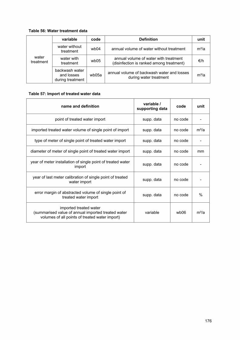
176

Table 56: Water treatment data

water treatment

variable code Definition unit

water without treatment wb04 annual volume of water without treatment m³/a

water with treatment wb05 annual volume of water with treatment

(disinfection is ranked among treatment) €/h

backwash water and losses

during treatment wb05a annual volume of backwash water and losses

during water treatment m³/a

Table 57: Import of treated water data

name and definition variable / supporting data code unit

point of treated water import supp. data no code -

imported treated water volume of single point of import supp. data no code m³/a

type of meter of single point of treated water import supp. data no code -

diameter of meter of single point of treated water import supp. data no code mm

year of meter installation of single point of treated water import supp. data no code -

year of last meter calibration of single point of treated water import supp. data no code -

error margin of abstracted volume of single point of treated water import supp. data no code %

imported treated water (summarised value of annual imported treated water

volumes of all points of treated water import) variable wb06 m³/a

177

Table 58: Returned water data

name and definition variable / supporting data code unit

point of returned water discharge supp. data no code -

returned water volume of single point of returned water discharge supp. data no code m³/a

type of meter of single point of returned water discharge supp. data no code -

diameter of meter of single point of returned water discharge supp. data no code mm

year of meter installation of single point of returned water discharge supp. data no code -

year of last meter calibration of single point of returned water discharge supp. data no code -

error margin of abstracted volume of single point of returned water discharge supp. data no code %

returned water (summarised value of annual returned water volumes of

all points of returned water discharge) variable wb22 m³/a

The system input volume (Table 59) is calculated out the previous described data: + total volume of abstracted water (wb01) + total volume of imported raw water (wb02) - volume of exported raw water (wb03) - backwash water and losses during treatment (wb05a) + volume of imported treated water (wb06) - volume of returned water (wb22) = system input volume (wb07) Table 59: System input data

variable code Definition unit

system input volume

wb07 [A3] annual volume of system input m³/a

[IWA Code], [IWA definition] and [IWA unit]…according to ALEGRE et al. (2006)

178

Table 60: Billed water consumption data

name and definition variable /

supporting data / context information

code unit

annual volume of unmetered exported treated water supp. data no code m³/a

point of treated water export supp. data no code -

treated exported water volume of single point of export supp. data no code m³/a

type of meter of single point of treated water export supp. data no code -

diameter of meter of single point of treated water export supp. data no code mm

year of meter installation of single point of treated water export supp. data no code -

year of last meter calibration of single point of treated water export supp. data no code -

error margin of abstracted volume of single point of treated water export supp. data no code %

exported treated water (summarised value of annual exported treated water volumes of all points of treated water export) variable wb08

[A7] m³/a

annual billed metered consumption (direct supply) supp. data no code m³/a

annual billed unmetered consumption (direct supply) supp. data no code m³/a

billed consumption (direct supply), (total amount of annual billed authorised consumption, only direct supply) variable wb09 m³/a

billed metered consumption [total amount of annual billed metered authorised

consumption (including exported water)] variable wb23

[A8] m³/a

billed unmetered consumption [total amount of annual billed unmetered authorised

consumption (including exported water)] variable wb24

[A9] m³/a

billed authorised consumption [total amount of annual billed authorised consumption

(including exported water)] variable wb16

[A10] m³/a

bulk water consumption (exported water to other water undertakings)

context information

ci21 [CI69] [%]

direct supply (residential, commercial, public and industrial consumption)

context information ci22 %

[IWA Code], [IWA definition] and [IWA unit]…according to ALEGRE et al. (2006)

179

Table 61: Unbilled water consumption data

name and definition variable / supporting data code unit

description of each unbilled metered consumption supp. data no code -

annual volume of each single unbilled metered consumption supp. data no code m³/a

unbilled metered consumption [total amount of annual unbilled metered consumption (including exported water)]

variable wb25 [A11] m³/a

description of each unbilled unmetered consumption supp. data no code -

annual volume of each single unbilled unmetered consumption supp. data no code m³/a

unbilled unmetered consumption [total amount of annual unbilled unmetered

authorised consumption (including exported water)] variable wb26

[A12] m³/a

unbilled authorised consumption [total amount of annual unbilled authorised

consumption (including exported water)] variable wb17

[A13] m³/a

[IWA Code], [IWA definition] and [IWA unit]…according to ALEGRE et al. (2006)

The annual authorised consumption (Table 62) is calculated out the previous described data: + billed authorised consumption (wb16) + unbilled authorised consumption (wb17) = authorised consumption (wb15) Table 62: Authorised consumption data

variable code Definition unit

authorised consumption

wb15 [A14]

annual volume of metered and/or non-metered water that is taken by registered customers, by the water

supplier itself or by others who are implicitly or explicitly authorised to do so by the water supplier,

for residential, commercial, industrial or public purposes; it includes water exported

m³/a

[IWA Code], [IWA definition] and [IWA unit]…according to ALEGRE et al. (2006)

180

The last part of water balance data deals with water losses. The volume of real (physical) water losses is calculated by: system input volume (wb07) - authorised consumption (wb15) - apparent losses (wb19) = real losses (wb20) Table 63: Water loss data

name and definition variable / supporting data code unit

possible meter errors of customer meters supp. data no code %

description of each type of unauthorised consumption supp. data no code -

volume of unauthorised consumption for each type of unauthorised consumption supp. data no code m³/a

total volume of authorised consumption (summarised value of authorised consumption

volumes of all types of unauthorised consumption) supp. data no code m³/a

water losses [difference between system input volume and

authorised consumption] variable wb18

[A15] m³/a

apparent losses (summarised value of annual volume of authorised

consumption and customer meter inaccuracies) variable wb19

[A18] m³/a

real losses [total amount of annual physical water losses up to

the point of customer metering] variable wb20

[A19] m³/a

Non-revenue water [difference between system input volume and

authorised consumption] variable wb21

[A21] m³/a

[IWA Code], [IWA definition] and [IWA unit]…according to ALEGRE et al. (2006)

A1.5. Process specific data In general, the assessment period for process specific data is three years to avoid pure comparability due to annual variations in process operation.

181

A1.5.1. Data of leakage monitoring sub process Table 64: Variables of leakage monitoring sub process

Variable Code Definition unit

total costs of sub process leakage monitoring v101

annual costs (personal and material) including costs for

outsourcing in-house and extern and fictive depreciation costs

€/a

total working time of sub process leakage monitoring v102

annual working time including working time of outsourcing

in-house and extern hours/a

working time utility intern of sub process leakage monitoring v103 annual working time for

sub process excluding outsourcing hours/a

personal costs utility intern of sub process leakage monitoring v104

annual utility intern personal costs for sub process excluding

outsourcing €/a

other costs utility intern for sub process leakage monitoring v105

annual other running costs and material costs utility intern for

sub process €/a

costs for outsourcing in-house for sub process leakage monitoring v106

annual costs (apportionments) for outsourcing in-house for

sub process €/a

working time outsourcing in-house of sub process leakage monitoring v107 annual working time of outsourcing

in-house for sub process hours/a

personal costs outsourcing in-house of sub process leakage monitoring v108

annual personal of costs outsourcing in-house for

sub process €/a

material costs outsourcing in-house of sub process leakage monitoring v109 annual material costs of outsourcing

in-house for sub process €/a

costs for outsourcing extern for sub process leakage monitoring v110

annual costs (apportionments) for outsourcing extern for

sub process €/a

working time outsourcing extern of sub process leakage monitoring v111 annual working time of outsourcing

extern for sub process hours/a

personal costs outsourcing extern of sub process leakage monitoring v112

annual personal of costs outsourcing extern for

sub process €/a

material costs outsourcing extern of sub process leakage monitoring v113 annual material costs of outsourcing

extern for sub process €/a

investment costs for leakage monitoring equipment v114

estimated costs of measurement equipment and SCADA system for those components or those parts of the SCADA system which accord to

leakage monitoring

€

average age of leakage monitoring system v115

estimated average age of leakage monitoring equipment and SCADA

system

a (years)

182

Table 65: Context information of leakage monitoring sub process

context information code definition / possible answer unit

system input metering ci101* 5 possible answers (low to high performance), see chapter 5.5 -

district metered areas (DMA) ci102* 5 possible answers (low to high performance), see chapter 5.5 -

evaluation of night minimum consumption ci103*

5 possible answers (low to high performance), see chapter 5.5 -

SCADA system ci104* 5 possible answers (low to high performance), see chapter 5.5 -

pressure monitoring ci105* 5 possible answers (low to high performance), see chapter 5.5 -

permanent noise loggers ci106* 5 possible answers (low to high performance), see chapter 5.5 -

virtual measuring zones ci107* 5 possible answers (low to high performance), see chapter 5.5 -

recognition of leakage ci108* 5 possible answers (low to high performance), see chapter 5.5 -

first information about leak location ci109* 5 possible answers (low to high performance), see chapter 5.5 -

function of SCADA system: transmission of system input data ci110* yes / no -

function of SCADA system: transmission interval of system input data ci111* 5 possible answers (low to high

performance), see chapter 5.5 -

function of SCADA system: transmission of DMA input data ci112* yes / no -

function of SCADA system: transmission interval of DMA input data ci113* 5 possible answers (low to high

performance), see chapter 5.5 -

function of SCADA system: transmission of pressure data ci114* yes / no -

function of SCADA system: transmission interval of pressure data ci115* 5 possible answers (low to high

performance), see chapter 5.5 -

function of SCADA system: transmission of reservoir water level ci116* yes / no -

function of SCADA system: transmission interval of reservoir water level ci117* 5 possible answers (low to high

performance), see chapter 5.5 -

function of SCADA system: transmission of pumping station data ci118* yes / no -

function of SCADA system: transmission interval of pumping station data ci119* 5 possible answers (low to high

performance), see chapter 5.5 -

function of SCADA system: evaluation of night minimum consumption ci120* yes / no -

function of SCADA system: automatic alarm when threshold values exceeded ci121* yes / no -

* considered in quality matrix

183

A1.5.2. Data of sub process leak detection Table 66: Variables to costs and working time of leak detection sub process

variable Code Definition unit

total costs of sub process leak detection v201

annual costs (personal and material) including costs for

outsourcing in-house and extern and fictive depreciation costs for

leak detection equipment

€/a

total working time of sub process leak detection v202

annual working time including working time of outsourcing

in-house and extern hours/a

working time utility intern of sub process leak detection v203 annual working time for

sub process excluding outsourcing hours/a

personal costs utility intern of sub process leak detection v204

annual utility intern personal costs for sub process excluding

outsourcing €/a

other costs utility intern for sub process leak detection v205

annual other running costs and material costs utility intern for

sub process €/a

costs for outsourcing in-house for sub process leak detection v206

annual costs (apportionments) for outsourcing in-house for

sub process €/a

working time outsourcing in-house of sub process leak detection v207 annual working time of outsourcing

in-house for sub process hours/a

personal costs outsourcing in-house of sub process leak detection v208

annual personal of costs outsourcing in-house for

sub process €/a

material costs outsourcing in-house of sub process leak detection v209 annual material costs of outsourcing

in-house for sub process €/a

costs for outsourcing extern for sub process leak detection v210

annual costs (apportionments) for outsourcing extern for

sub process €/a

working time outsourcing extern of sub process leak detection v211 annual working time of outsourcing

extern for sub process hours/a

personal costs outsourcing extern of sub process leak detection v212

annual personal of costs outsourcing extern for

sub process €/a

material costs outsourcing extern of sub process leak detection v213 annual material costs of outsourcing

extern for sub process €/a

184

Table 67: Variables for existing leak detection equipment

Variable code Definition unit

listening sticks and stethoscopes v216

number of leak detection equipment within the utility

-

ground microphones v217 -

leak noise correlators v218 -

temporary noise loggers v219 -

equipment for tracer gas v220 -

measuring vehicles v221 -

other leak detection equipment v222 -

description of other leak detection equipment v223 - -

investment costs for leak detection equipment v224 estimated investment costs of leak

detection equipment €

depreciation costs for leak detection equipment v225

annual fictive depreciation costs calculated on basis of a

depreciation period of 10 years €/a

Table 68: Variables for localised leaks

variable code unit

localised leaks in assessment

period (3 years)

leaks at transmission mains (routine survey) v239 -

leaks at transmission mains (cause based) v240 -

leaks at distribution mains (routine survey) v242 -

leaks at distribution mains (cause based) v243 -

leaks at service connections (routine survey) v245 -

leaks at service connections (cause based) v246 -

185

Table 69: Variables for leak detection measures in assessment period

variable code definition unit

leak detection equipment used in assessment

period (3 years)

listening sticks and stethoscopes v226

Was this leak detection equipment used in the assessment period?

-

ground microphones v227 -

leak noise correlators v228 -

temporary noise loggers v229 -

equipment for tracer gas v230 -

step testing v231 -

Other leak detection equipment v232 -

description of other leak detection equipment v233 - -

leak detection measures in assessment

period (3 years)

leak detection on transmission mains (routine survey) v234a

length of transmission / distribution mains

inspected by leak detection measures in routine

surveys / cause related during assessment period

km

leak detection on transmission mains (cause related) v234b km

leak detection on distribution mains (routine survey) v234c km

leak detection on distribution mains (cause related) v234d km

cost of routine leak detection survey v235

part of sub process running costs (without depreciation

costs for leak detection equipment) for routine

surveys

€

cost of cause related leak detection v236

part of sub process running costs (without depreciation

costs for leak detection equipment) for cause related leak detection

€

inspected service connections (routine survey) v237

number of service connections inspected for leakage by routine surveys during assessment period

-

inspected service connections (cause related) v237a

number of service connections inspected for

leakage cause related during assessment period

-

186

Table 70: Context information for leak detection sub process

context information code definition / possible answer unit

general procedure in leak detection (strategy) ci201* 5 possible answers (low to high

performance), see chapter 5.5 -

routine leak detection at service connections ci201a*

Is routine leak detection at service connections done together with

customer meter reading (or meter replacement)?

-

leak location time ci202* 5 possible answers (low to high performance), see chapter 5.5 -

hit rate (success in leak detection) ci203* 5 possible answers (low to high performance), see chapter 5.5 -

accuracy in pinpointing leaks ci204* 5 possible answers (low to high performance), see chapter 5.5 -

documentation of leak detection ci205* 5 possible answers (low to high performance), see chapter 5.5 -

service connection plastic material ci206 service connections of material PVC, Pe or GRP %

service connection metallic material ci207 service connections of material steel, GG, GGG, (lead) %

Your personal opinion: Do routine inspections on leakage at service

connections together with meter readings (or meter replacement) pay off?

ci208 yes / no -

Are those materials suitable for detecting leaks?

PVC ci210 4 possible answers:

very suitable, high hit rate moderate suitable, average hit rate

not very suitable, low hit rate not suitable at all, no leaks found

-

PE ci211 -

Steel ci212 -

CI ci213 -

others ci214 -

name of “other” material ci215 description of “other material” of k214 -

payment criteria for contracted leak detection companies ci216

5 possible answers: flat sum for whole leak detection

inspected mains length working time

success of leak detection others

-

soil conditions

cohesive (clay, silt) ci218 ratio of mains in cohesive soil %

cohesionless (sand, gravel) ci219 ratio of mains in cohesionless soil %

leaks coming to surface ci220 estimation of percentage of leaks

coming to surface due to soil conditions

%

* considered in quality matrix

187

A1.5.3. Data for analyses and planning sub process Table 71: Variables for costs and work time of analyses and planning sub process

Variable code definition unit

total costs of sub process analyses and planning v301

annual costs (personal and material) including costs for

outsourcing in-house and extern for sub process

€/a

total working time of sub process analyses and planning v302

annual working time including working time of outsourcing

in-house and extern hours/a

working time utility intern of sub process analyses and planning v303 annual working time for

sub process excluding outsourcing hours/a

personal costs utility intern of sub process analyses and planning v304

annual utility intern personal costs for sub process excluding

outsourcing €/a

other costs utility intern for sub process analyses and planning v305

annual other running costs and material costs utility intern for

sub process €/a

costs for outsourcing in-house for sub process analyses and planning v306

annual costs (apportionments) for outsourcing in-house for

sub process €/a

working time outsourcing in-house of sub process analyses and planning v307 annual working time of outsourcing

in-house for sub process hours/a

personal costs outsourcing in-house of sub process analyses and planning v308

annual personal of costs outsourcing in-house for

sub process €/a

material costs outsourcing in-house of sub process analyses and planning v309 annual material costs of outsourcing

in-house for sub process €/a

costs for outsourcing extern for sub process analyses and planning v310

annual costs (apportionments) for outsourcing extern for

sub process €/a

working time outsourcing extern of sub process analyses and planning v311 annual working time of outsourcing

extern for sub process hours/a

personal costs outsourcing extern of sub process analyses and planning v312

annual personal of costs outsourcing extern for

sub process €/a

material costs outsourcing extern of sub process analyses and planning v313 annual material costs of outsourcing

extern for sub process €/a

188

Table 72: Context information for analyses and planning (part 1)

context information code definition / possible answer unit

general procedure in analyses and planning ci301* 5 possible answers (low to high performance), see chapter 5.5 -

time interval in

which different

criteria are analysed

or planned

calculation of water loss PIs for whole supply system ci302*

5 possible answers:

never done up to now more than 5 years each 2 to 5 years

annual or every half year quarterly, monthly or more often

-

calculation of water loss PIs for single DMAs ci303* -

analyses to trends in night minimum consumption of

single zones ci304* -

investigations if existing measuring systems (flow, pressure etc.) and SCADA

systems are sufficient

ci305* -

internal analyses of costs (efficiency) and success (affectivity) of water loss

management

ci306* -

derivation of measures for improvement of process operation (e.g. working

instructions)

ci307* -

generation of failure statistics for whole supply system

without analyses of single pipe-groups

ci308* -

generation of failure statistics for single DMAs without

analyses of single pipe-groups ci309*

generation of failure statistics for whole supply system with

analyses of single pipe-groups ci310* -

generation of failure statistics for single DMAs with analyses

of single pipe-groups ci311* -

derivation of measures for improvement in maintenance (e.g. for critical pipe groups)

ci312* -

provision of pipe-group based failure statistics for

rehabilitation planning ci313* -

* considered in quality matrix

189

Table 73: Context information for analyses and planning (part 2)

context information code definition / possible answer unit

calculation of water loss performance indicators ci314* 5 possible answers (low to high

performance), see chapter 5.5 -

PIs calculated for

internal purposes

water loss ratio (%) ci315* yes / no -

real losses per connection per day ci316* yes / no -

real losses per connection per day per metre pressure ci317* yes / no -

real losses per mains length ci318* yes / no -

ILI ci319* yes / no -

non-revenue water (NRW) (%) ci320* yes / no -

PIs published in annual

report (e.g. for

stakeholders)

water loss ratio (%) ci321* yes / no -

real losses per connection per day ci322* yes / no -

real losses per connection per day per metre pressure ci323* yes / no -

real losses per mains length ci324* yes / no -

ILI ci325* yes / no -

non-revenue water (NRW) (%) ci326* yes / no -

calculation of a water balance ci327* 5 possible answers (low to high performance), see chapter 5.5 -

* considered in quality matrix

190

A1.5.4. Data for infrastructure management supporting process Table 74: Context information for infrastructure management supporting process

context information code definition / possible answer unit

mapping / GIS ci401* 5 possible answers (low to high performance), see chapter 5.5 -

network inspection

inspection intervals

closing valves ci402*

5 possible answers (low to high performance), see chapter 5.5

-

hydrants ci403* -

pressure reduction valves ci404* -

calibration interval system input meters ci405* -

calibration interval DMA meters ci406* -

hydraulic modelling

accomplishment of hydraulic modelling ci407* 5 possible answers (low to high

performance), see chapter 5.5 -

Were new leaks found due to results of hydraulic modelling? ci408 yes / no -

Were optimisation potentials in pressure management investigated

by hydraulic modelling? ci409* yes / no -

pressure management ci410* 5 possible answers (low to high performance), see chapter 5.5 -

rehabilitation

rehabilitation planning ci411* 5 possible answers (low to high performance), see chapter 5.5 -

rehabili-tation criteria

experience of network engineer ci412* yes / no -

failure rates ci413* yes / no -

water losses ci414* yes / no -

other underground work ci415* together with other measures

e.g. street renewal -

IT support ci416* yes / no -

average age of distribution mains ci417 average age -

average rehabilitation rate of distribution mains ci418 average rehabilitation rate within

the last 10 years %

average age of service connections ci419 average age -

average rehabilitation rate of service connections ci420 average rehabilitation rate within

the last 10 years %

customer meter

management

metering equipment ci421*

5 possible answers (low to high performance), see chapter 5.5

-

meter age and replacement interval ci422* -

time frame for meter readings ci423* -

theft of water, illegal connections, bypasses, manipulations ci424* -

* considered in quality matrix

191

A1.5.4.1.1. Data for leak repair supporting process Table 75: Variables about number of repairs and repair costs

context information code definition / possible answer unit

number of repairs of

pipe failures

at transportation mains v501

total number of repairs for failures at pipes or fittings (with

leakage) during assessment period

-

at distribution mains v502 -

at service connections v503 -

number of repairs of

fitting failures

at transportation mains v504 -

at distribution mains v505 -

at service connections v506 -

total repair costs of pipe

failures

at transportation mains v507

total costs (earthwork, installation, material etc.) of repairs of failures at pipes or fittings (with leakage) during

assessment period

€

at distribution mains v508 €

at service connections v509 €

total repair costs of fitting

failures

at transportation mains v510 €

at distribution mains v511 €

at service connections v512 €

Table 76: Context information about repair time and information for planning

context information code definition / possible answer unit

repair time

reported leaks at distribution mains ci501* time from locating a leak to the recovery of the functionality of

the pipe 5 possible answers (low to high performance), see chapter 5.5

-

unreported leaks at distribution mains ci502* -

reported leaks at service connections ci503* -

unreported leaks at service connections ci504* -

Does it happen that leaks are located but repaired weeks or month later? ci505* yes / no -

information for maintenance and rehabilitation planning ci506* 5 possible answers (low to high

performance), see chapter 5.5 -

* considered in quality matrix

192

Table 77: Context information about failure documentation

context information code definition / possible answer unit

modality of failure documentation ci507* 5 possible answers (low to high performance), see chapter 5.5 -

criteria of failure

documentation

(according to OVGW

guideline W 100)

name of documenting person ci508*

yes / no

Which of these single criteria are documented for each single

repair?

-

place and time of failure ci509* -

year of construction ci510* -

pipe diameter ci511* -

type of pipe (transportation or distribution main, service

connection) ci512* -

pipe material ci513* -

pipe connection ci514* -

corrosion protection ci515* -

affected part (pipe, fitting, connection) ci516* -

condition of pipe and bedding ci517* -

type of failure (burst, fitting…) ci518* -

cause of failure (e.g. corrosion) ci519* -

sketch of position, photo documentation ci520* -

process of failure elimination ci521* -

type of repair / maintenance ci522* -

costs of repair ci523* -

* considered in quality matrix

193

Table 78: Context information about type of failures

context information code definition / possible answer unit

type of failures (only failures with leakage)

transportation mains

burst ci524

percentages for type of failures with leakage at

transportation mains (sum has to be 100%)

%

crack ci525 %

hole ci526 %

connection failure ci527 %

fitting failure ci528 %

others ci529 %

distribution mains

burst ci530

percentages for type of failures with leakage at

distribution mains (sum has to be 100%)

%

crack ci531 %

hole ci532 %

connection failure ci533 %

fitting failure ci534 %

others ci535 %

service connections

burst ci536

percentages for type of failures with leakage at

service connections (sum has to be 100%)

%

crack ci537 %

hole ci538 %

connection failure ci539 %

fitting failure ci540 %

others ci541 %

194

Table 79: Context information about cause of failures

context information code definition / possible answer unit

cause of failure

(only failures with leakage)

transportation mains

corrosion ci542

percentages of causes for failures with leakage at

transportation mains (sum has to be 100%)

%

settlings ci543 %

material or installation failure ci544 %

freezing ci545 %

fatigue of material ci546 %

external forces ci547 %

others ci548 %

distribution mains

corrosion ci549

percentages of causes for failures with leakage at

distribution mains (sum has to be 100%)

%

settlings ci550 %

material or installation failure ci551 %

freezing ci552 %

fatigue of material ci553 %

external forces ci554 %

others ci555 %

service connections

corrosion ci556

percentages of causes for failures with leakage at

service connections (sum has to be 100%)

%

settlings ci557 %

material or installation failure ci558 %

freezing ci559 %

fatigue of material ci560 %

external forces ci561 %

others ci562 %

195

A1.5.5. Data for qualification of staff supporting process Table 80: Context information about qualification of staff

context information code definition / possible answer unit

employees who are proved water masters ci601*

y/n

-

employees with special training course an water loss management ci602* -

employees with experience in using listening sticks and stethoscopes ci603* -

employees with experience in using ground microphones ci604* -

employees with experience in using leak noise correlators ci605* -

employees with experience in using noise loggers ci606* -

employees with experience in using tracer gas ci607* -

employees with experience in evaluation of zonal (or DMA) measurements ci608* -

employees with experience in evaluation of night minimum consumption ci609* -

employees with experience in pipe group based failure statistics ci610* -

operation of hydraulic modelling ci611* personnel of utility / external personal -

procedure in advanced staff training ci612* 5 possible answers (low to high performance), see chapter 5.5 -

* considered in quality matrix

Veröffentlichungen

I

Mitteilungen des Institutes für Wasserwirtschaft und Konstruktiven Wasserbau der Technischen Universität Graz

Bisher erschienene Hefte: Heft 1 (1959) VEDER, Ch.: Neue Verfahren zur Herstellung von untertägigen Wän-

den und Injektionsschirmen in Lockergesteinen und durchlässigem Fels (vergriffen)

Heft 2 (1959) BEER, O.: Hochwasserentlastungsanlagen österreichischer Talsperren Heft 3 (1960) WEHRSCHÜTZ, F.: Wasserentnahme aus alpinen Abflüssen Heft 4 (1961) TSCHADA, H.: Die Spiralenauslässe des Kraftwerkes St.Pantaleon Heft 5 (1962) GRENGG, H.: Funktion, Ordnung und Gestalt im konstruktiven Was-

serbau Heft 6 (1962) PIRCHER, W.: Wehreichungen an der Enns Heft 7 (1962) WEHRSCHÜTZ, F.: Füll- und Entleerungssysteme von Schiffs-

schleusen mit großen Fallhöhen Heft 8 (1962) REITZ, A.: Das Stauwerk im Bogen Heft 9 (1963) PIRCHER, W.: Die Bautypen der Wasserkraft Heft 10 (1964) WEHRSCHÜTZ, F.: Kritische Betrachtung der Modellgesetze Heft 11 (1965) SIMMLER, H.: Das neue Institut für Wasserbau Heft 12 (1964) RADLER, S.: Die Berechnung der Abflüsse im natürlichen Gerinne Heft 13 (1965) ALTENBURGER, H.: Der Spiralauslaß als Hochwasserentlastung bei

Donaukraftwerken Heft 14 (1965) KRESNIK, E.: Kunststoffe im wasserbaulichen Versuchswesen und

deren rauhigkeitsmäßige Erfassung Heft 15 (1970) SVEE, R.: Untersuchungen über die Stabilität bei Wasserkraftanlagen

mit idealer Regelung Heft 16 (1971) DROBIR, H.: Die Registrierung eines zeitlich rasch veränderlichen

Wasserspiegels mit kapazitiven Meßsonden ROTH, G.: Meßanlage zum Studium instationärer Vorgänge mit Hilfe

eines Digitalcomputers Heft 17 (1971) DROBIR, H.: Der Ausfluß aus einem Speicher beim Bruch einer Tal-

sperre Heft 18 (1972) GRENGG, H.: Wörterbuch der Wasserkraftnutzung; Französisch – Deutsch, Deutsch – Französisch Heft 19 (1973) DRAXLER, A.: Mathematisches Modell für die Zuflußprognose als

Hilfsmittel zur Optimierung des KW-Betriebes Heft 20 (1974) GRENGG, H.: Die Technisierung großer Ströme in Verbindung mit

der Wasserkraft Heft 21 (1975) GRENGG, H.: Die großen Wasserkraftanlagen des Weltbestandes Heft 22 (1977) GRENGG, H.: Die großen Wasserkraftanlagen des Weltbestandes, 2.

Teil KRAUSS, H.: Lufteinzug durch den Wasserabfluß in Vertikalrohren

Veröffentlichungen

II

Heft 23 (1979) LIEBL, A.: Die Lehre aus der Katastrophe beim Aufstau des Tarbela-Dammes in Pakistan aus der Sicht der Stahlwasserbauer

(1980) KRÖLL, A.: Die Stabilität von Steinschüttungen bei Sohlen- und Uferbefestigungen in Wasserströmungen

Heft 24 (1981) TSCHERNUTTER, P.: Grundsatzüberlegungen zur Rentabilität und zum Ausbau von Kleinwasserkraftwerken

Heft 25 (1984) Helmut Simmler – Zur Vollendung seines 65.Lebensjahres gewidmet von seinen ehemaligen und derzeitigen Mitarbeitern an der TU Graz

Publikation des Institutes für Hydromechanik, Hydraulik und Hydrologie der Technischen Universität Graz

Bisher erschienene Bände: SACKL, B. (1987) Ermittlung von Hochwasser - Bemessungsganglinien in

beobachteten und unbeobachteten Einzugsgebieten

Veröffentlichungen des Institutes für Siedlungs- und Industriewasser-wirtschaft, Grundwasserhydraulik, Schutz- und Landwirtschaftlichen Wasserbau der Technischen Universität Graz

Bisher erschienene Bände: Band 1 (1977) RENNER, H.: Die Berücksichtigung nichtbindiger überdeckender

Schichten bei der Bemessung von Wasserschutzgebieten Band 2 (1977) KAUCH, E.P.: Untersuchung des Bewegungsgesetzes für die Filter-

strömung, im besonderen bei höheren Geschwindigkeiten ein-schließlich der teilturbulenten Strömung

Band 3 (1977) PONN, J.: Geschwindigkeitsverteilungen in radial durchströmten Nachklärbecken – Verwendung einer neu entwickelten Thermosonde

Band 4 (1978) Festschrift zum 60. Geburtstag von E.P. Nemecek Band 5 (1979) RENNER, H.: Die Entwicklung einer biologischen Kläranlage für

kleinste Verhältnisse Band 6 (1980) Forschungsberichte 1979/80 Band 7 (1980) KAUCH, E.P.: Der Pumpversuch im ungespannten Grundwasserleiter Band 8 (1982) DITSIOS, M.: Untersuchungen über die erforderliche Tiefe von

horizontal durchströmten rechteckigen Nachklärbecken von Belebungsanlagen

Band 9 (1982) GEIGER, D.: Einfluß der Schlammräumung im Nachklärbecken auf die erreichbare Feststoffkonzentration im Belebungsbecken

Band 10 (1984) Forschungsbericht 1983/84 (vergriffen) Band 11 (1984) Beeinträchtigung der Grundwasservorkommen in qualitativer und

quantitativer Hinsicht Band 12 (1986) KOTOULAS, K.: Natürliche Entwicklung der Längen- und Quer-

profilform der Flüsse - ein Beitrag zum naturnahen Flußbau

Veröffentlichungen

III

Band 13 (1987) KAUCH, E.P., M. DITSIOS: Schlammbilanz in Belebungsanlagen - Einfluß der hydraulischen Betriebsparameter für Trockenwetter- und Regenwetterfall

Band 14 (1988) Festschrift zum 70. Geburtstag von Ernst P. Nemecek Band 15 (1988) Vorträge über Siedlungs- und Industriewasserbau Band 16 (1991) KAINZ, H.: Auswirkungen von Stoßbelastungen auf den Feststoff-

haushalt einer Belebungsanlage Band 17 (1991) KLAMBAUER, B.: Grundwasserschutz und Landwirtschaft –

Situation in Mitteleuropa

Schriftenreihe zur Wasserwirtschaft Technische Universität Graz

Bisher erschienene Bände: Band 1 (1992) Hermann Grengg – zum 100. Geburtstag 1) Band 2 (1992) ZITZ, W.: Die Mitbehandlung angefaulter Sammelgrubenabwässer in

einer kommunalen, schwach belasteten Belebungsanlage 2), vergriffen Band 3 (1992) ÜBERWIMMER, F.: Untersuchung der Ressourcen gespannter

Grundwassersysteme mit hydraulischen und hydrologischen Modellen 1), 2)

Band 4 (1992) Hochwasserrückhaltebecken – Planung, Bau und Betrieb 1), 2) Band 5 (1992) MOLNAR, T.: Rechnerunterstütztes Projektieren von Bewässerungs-

systemen 1), 2) Band 6 (1993) Klärschlammentsorgung in der Steiermark 2) Band 7 (1993) FRIEDRICH, Ch., WINDER, O.: Lebensraum Grazer Murböschun-

gen – Zoologisch-botanische Untersuchungen einschließlich Planungsvorschläge 2)

Band 8 (1993) REICHL, W.: Mehrdimensionale Optimierung quantitativ und qualitativ bewertbarer Zielfunktionen in der Wasserwirtschaft 1)

Band 9 (1993) WELLACHER, J.: Instationäre Strömungsvorgänge in Hochwasser-rückhaltebecken 1)

Band 10 (1993) STUBENVOLL, H. : Analyse der zeitlichen Struktur von Niederschlagsereignissen auf der Grundlage zeitvariabler Daten-aufzeichnung;

ZEYRINGER, T.: Untersuchung des räumlichen Verhaltens von Niederschlagsereignissen auf zeitvariabler Datengrundlage 1), 2)

Band 11 (1993) Ingenieurbiologie im Schutzwasserbau 2) Band 12 (1994) Ländlicher Raum: Abwasserentsorgung in der Sackgasse? 2)

(vergriffen) Band 13 (1994) SACKL, B.: Ermittlung von Hochwasser-Bemessungsganglinien in

beobachteten und unbeobachteten Einzugsgebieten 1), 2) Band 14 (1995) Leben mit dem Hochwasser – Gefahr und Anpassung 2) Band 15 (1995) Betrieb, Erhaltung und Erneuerung von Talsperren und

Hochdruckanlagen – Symposium 1) Band 16 (1995) RICHTIG, G.: Untersuchungen zur Abflußentstehung bei

Hochwasserereignissen in kleinen Einzugsgebieten 2)

Veröffentlichungen

IV

Band 17 (1995) KNOBLAUCH, H.: Dissipationsvorgänge in Rohrleitungssystemen 1) Band 18 (1995) Fremdwasser in Abwasseranlagen 2) Band 19/1 (1996) XVIII. Konferenz der Donauländer über hydrologische Band 19/2 Vorhersagen und hydrologisch-wasserwirtschaftliche Grundlagen 1), 2) Band 20 (1996) STRANNER, H.: Schwallwellen im Unterwasser von

Spitzenkraftwerken und deren Reduktion durch flußbauliche Maßnahmen 1)

Band 21 (1996) DUM, T.: Verifikation eines numerischen Strömungsmodells anhand physikalischer Modelle 1)

Band 22 (1996) VASVÁRI, V.: Ein numerisches Modell zur Bewirtschaftung gespannter Grundwasservorkommen am Beispiel des Mittleren Safentales 1), 2)

Band 23 (1996) HYDROLOGISCHE MONOGRAPHIE des Einzugsgebietes der Oberen Raab 1), 2)

Band 24 (1997) Niederwasser 1), 2) Band 25 (1997) KRALL, E.: Untersuchung der Gesamtwahrscheinlichkeit von

Hochwasserereignissen in kleinen, unbeobachteten Einzugsgebieten Österreichs auf der Grundlage von Gebietskennwerten 1), 2)

Band 26 (1997) Abwasserentsorgung bei fehlenden Vorflutern 2) Band 27 (1997) Festschrift anläßlich des 60. Geburtstages von Herrn O.Univ.-Prof.

Dipl.-Ing. Dr. techn. Günther Heigerth 1) Band 28 (1997) MEDVED, N.: Simulation und systematische Erfassung von

Spülvorgängen in verlandeten Flussstauräumen 1) Band 29 (1998) Festschrift anläßlich des 65. Geburtstages von Herrn O.Univ.-Prof.

Dipl.-Ing. Dr. techn. Dr.h.c. Heinz Bergmann 1), 2) Band 30 (1998) Festschrift anläßlich des 80. Geburtstages von Herrn em.O.Univ.-Prof.

Dipl.-Ing. Dr.h.c. Dr. techn. Ernst P. Nemecek 2) Band 31 (1999) BEUTLE, K.: Untersuchungen zur Schlammstabilisierung bei

diskontinuierlich belüfteten Belebungsanlagen 2) Band 32 (1999) REINHOFER, M.: Klärschlammvererdung mit Schilf 2) Band 33 (1999) GRUBER, G.: Der biologisch abbaubare Kohlenstoffgehalt in der

Abwassertechnik, BTOC und BDOC als Alternative zum BSB 2) Band 34 (2000) Betrieb und Überwachung wasserbaulicher Anlagen - Symposium 1) Band 35 (2001) FUCHS, D.: Decision Support Systeme für die Rehabilitationsplanung

von Wasserrohrnetzen 2) Band 36 (2001) Untersuchungen im Einzugsgebiet der Oberen Raab über

hydrologische Folgen einer möglichen Klimaänderung 1), 2) Band 37 (2001) HABLE, O.: Multidimensional probabilistic design concept for the

estimation of the overtopping probability of dams 1), 2)

Band 38 (2001) VASVÁRI, V.: Geohydraulische und bohrlochgeophysikalische Untersuchungen in geklüfteten Grundwasserleitern 1), 2)

Band 39 (2002) SCHATZL, R.: Skalenabhängiger Vergleich zwischen Wetterradar-daten und Niederschlagsmessungen 2)

Veröffentlichungen

V

Band 40 (2002) GUNDACKER, F.: Untersuchungen zur Schlammstabilisierung bei diskontinuierlich belüfteten Belebungsanlagen bei tiefen Temperaturen 2)

Band 41 (2003) Wasserbau neu – Die Wasserbauschule an der Technischen Universität Graz 2)

Band 42 (2004) Innovative Messtechnik in der Wasserwirtschaft – Konzeption und Praxiserfahrungen mit einem modularen Monitoringnetzwerk zur universellen Anwendung in der Wasserwirtschaft 2)

Band 43 (2005) 7. Treffen junger Wissenschaftlerinnen und Wissenschaftler deutschsprachiger Wasserbauinstitute 1)

Band 44 (2005) HOCHEDLINGER, M.: Assessment of Combined Sewer Overflow Emissions 2)

Band 45 (2006) NEMECEK, E.P., H.HAERTL, H.GERNEDEL und H.NICKL: Horizontalfilterbrunnen 2)

Band 46 (2006) WASSERBAUSYMPOSIUM GRAZ 2006 Stauhaltungen und Speicher – Von der Tradition zur Moderne 1)

Band 47 (2006) KAN((¦))FUNK – Überprüfung, Bewertung und Sicherstellung der Funktionsfähigkeit von Kanalisationsanlagen in Österreich 2)

Band 48 (2007) PATZIGER, M.: Untersuchung der Schlammbilanz in Belebungsstufen aufbauend auf den Prozessen im Nachklärbecken 2)

Band 49 (2007) Abwassergebührensplitting, ÖWAV – TU Graz Seminar 2)

Band 50 (2007) dex Fachsymposium 2007 – Abwasserableitung, Abwasser- und Klärschlammbehandlung 2)

Band 51 (2008) BADURA, H.: Feststofftransportprozesse während Spülungen von Flussstauräumen am Beispiel der oberen Mur 1)

Band 52 (2008) ARCH, A.: Luftein- und Austragsprozesse bei Anlagen mit Peltonturbinen im Gegendruckbetrieb 1)

Band 53 (2008) GANGL, G.: Rehabilitationsplanung von Trinkwassernetzen 2)

Band 54 (2008) Instandhaltung von Trinkwasser- und Abwasserleitungen; ÖWAV –TU Graz Symposium 2)

Band 55 (2009) Optimierte Bemessung von Mischwasserentlastungsanlagen, Erfahrungen mit der Anwendung des neuen ÖWAV-Regelblattes 19; ÖWAV – TU Graz Seminar 2)

Band 56 (2009) KOELBL, J.: Process Benchmarking in Water Supply Sector: Management of Physical Water Losses 2)

Die Bände sind zu beziehen bei: 1) Institut für Wasserbau und Wasserwirtschaft

Technische Universität Graz, Stremayrgasse 10/II, A-8010 Graz Tel. +43(0)316/873-8361, Fax +43(0)316/873-8357 E-Mail: hydro@tugraz.at

2) Institut für Siedlungswasserwirtschaft und Landschaftswasserbau Technische Universität Graz, Stremayrgasse 10/I, A-8010 Graz Tel. +43(0)316/873-8371, Fax +43(0)316/873-8376 E-Mail: office@sww.tugraz.at