Scheduling learning dependent jobs in customised assembly lines

This article was downloaded by: [University of California, Riverside Libraries]On: 08 October 2014, At: 14:39Publisher: Taylor & FrancisInforma Ltd Registered in England and Wales Registered Number: 1072954 Registeredoffice: Mortimer House, 37-41 Mortimer Street, London W1T 3JH, UK

International Journal of ProductionResearchPublication details, including instructions for authors andsubscription information:http://www.tandfonline.com/loi/tprs20

Scheduling learning dependent jobs incustomised assembly linesM.J. Anzanello a & F.S. Fogliatto ba Industrial and Systems Engineering Department , RUTGERSUniversity , 793 Bevier Road, Piscataway, NJ, 08854, USAb Industrial Engineering Department , Federal University of RioGrande do Sul , Avenida Osvaldo Aranha, 99, 5 andar, PortoAlegre, RS, 90035-90, BrasilPublished online: 09 Dec 2009.

To cite this article: M.J. Anzanello & F.S. Fogliatto (2010) Scheduling learning dependent jobs incustomised assembly lines, International Journal of Production Research, 48:22, 6683-6699

To link to this article: http://dx.doi.org/10.1080/00207540903307599

PLEASE SCROLL DOWN FOR ARTICLE

Taylor & Francis makes every effort to ensure the accuracy of all the information (the“Content”) contained in the publications on our platform. However, Taylor & Francis,our agents, and our licensors make no representations or warranties whatsoever as tothe accuracy, completeness, or suitability for any purpose of the Content. Any opinionsand views expressed in this publication are the opinions and views of the authors,and are not the views of or endorsed by Taylor & Francis. The accuracy of the Contentshould not be relied upon and should be independently verified with primary sourcesof information. Taylor and Francis shall not be liable for any losses, actions, claims,proceedings, demands, costs, expenses, damages, and other liabilities whatsoever orhowsoever caused arising directly or indirectly in connection with, in relation to or arisingout of the use of the Content.

This article may be used for research, teaching, and private study purposes. Anysubstantial or systematic reproduction, redistribution, reselling, loan, sub-licensing,systematic supply, or distribution in any form to anyone is expressly forbidden. Terms &Conditions of access and use can be found at http://www.tandfonline.com/page/terms-and-conditions

http://www.tandfonline.com/loi/tprs20

http://dx.doi.org/10.1080/00207540903307599

http://www.tandfonline.com/page/terms-and-conditions

http://www.tandfonline.com/page/terms-and-conditions

International Journal of Production ResearchVol. 48, No. 22, 15 November 2010, 6683–6699

Scheduling learning dependent jobs in customised assembly lines

M.J. Anzanelloa* and F.S. Fogliattob

aIndustrial and Systems Engineering Department, RUTGERS University, 793 Bevier Road,Piscataway, NJ, 08854, USA; bIndustrial Engineering Department, Federal University of RioGrande do Sul, Avenida Osvaldo Aranha, 99, 5 andar, Porto Alegre, RS, 90035-90, Brasil

(Received 7 February 2009; final version received 31 August 2009)

The large variety of product models required by customised markets implies lotsize reduction. This strongly affects manual-based production activities, sinceworkers need to promptly adapt to the specifications of the next model to beproduced. Completion times of manual-based activities tend to be highly variableamong workers, and are difficult to estimate. This affects the scheduling of thoseactivities since scheduling precision depends on reliable estimates of jobcompletion times. This paper presents a method that combines learning curvesand job scheduling heuristics aimed at minimising the total weighted earliness andtardiness. Workers performance data is collected and modelled using learningcurves, enabling a better estimation of the completion time of jobs with differentsize and complexity. Estimated completion times are then inputted in newscheduling heuristics for unrelated parallel workers, equivalent to machines in thisstudy, created by modifying heuristics available in the literature. Performance ofthe proposed heuristics is assessed analysing the difference between the optimalschedule objective function value and that obtained using the heuristics, as well asthe workload imbalance among workers. Some contributions in this paper are:(i) use of learning curves to estimate completion times of jobs with different sizesand complexities from different teams of workers; and (ii) use of a more complexscheduling objective function, namely the total weighted earliness and tardiness,as opposed to most of the developments in the current scheduling literature.A shoe manufacturing application illustrates the developments in the paper.

Keywords: learning curves; scheduling; unrelated parallel machines

1. Introduction

In mass customised environments a large variety of product models are manufacturedwith reduced lot sizes, demanding high flexibility of productive resources to enable fastadaptation to the new model to be produced (Da Silveira et al. 2001). Small lot productionof different products may generate losses in manual-based operations, as workers’ skillsmust promptly adapt to the features of the new model to minimise production disruptions.In such a context job scheduling becomes particularly difficult since the time to lotcompletion when the learning process is taking place is usually unknown. That creates aproduction scenario that could potentially benefit from the integration of learning curve(LC) modelling and scheduling techniques.

*Corresponding author. Email: [email protected]

ISSN 0020–7543 print/ISSN 1366–588X online

� 2010 Taylor & Francis

DOI: 10.1080/00207540903307599

http://www.informaworld.com

Dow

nloa

ded

by [

Uni

vers

ity o

f C

alif

orni

a, R

iver

side

Lib

rari

es]

at 1

4:39

08

Oct

ober

201

4

LCs are non-linear regression models associating workers performance, usually givenin terms of units produced per time interval, to task characteristics. LC modelling aims atdescribing the learning profile of workers (or teams of workers), depicting how efficiencyimproves as an operation is continuously repeated (Uzumeri and Nembhard 1998).

Job scheduling in manufacturing and in the service industry is an important researchtopic in the literature. In short it aims at allocating jobs to resources by optimising anobjective (Pinedo 2008). However, it seems that understanding the impacts of workerslearning on the scheduling framework has only recently become a research topic. Pioneerinvestigation was developed by Biskup (1999) analysing the effects of learning on theposition of jobs in a single machine. More recently Mosheiov and Sidney (2003) integratedjob dependent LCs, which are LCs displaying different parameters for each job, toscheduling formulations. The goal was to minimise simple objective functions such asflow-time and makespan on a single machine, as well as flow-time in unrelated parallelmachines.

In Mosheiov and Sidney (2003) job completion times were simulated assuming auniform distribution. However, probability distributions may not properly reflectprocessing times that present a functional pattern, as in learning situations. The needfor a better method to estimate job completion times in those situations becomes evidentif more efficient scheduling schemes are desired. A second drawback in Mosheiov andSidney’s (2003) work must also be addressed: they approached the scheduling problemusing simple scheduling objective functions, such as flow-time and makespan minimisa-tion. In real applications simultaneous optimisation with respect to earliness and tardinessis virtually mandatory, since delivering an item much earlier or later than its due dateincurs penalties (Adamopoulos and Pappis 1998).

This paper deals with scheduling problems where job completion times are dependenton the workers learning process, and where a total weighted earliness and tardinessobjective function is to be optimised. We first use a hyperbolic LC model to quantitativelyassess workers’ adaptation to a given set of jobs, with different complexities. Workers’learning profiles are then used to estimate processing times of new jobs. In our approacheach worker is considered as an unrelated parallel machine, since the rate of job executiondiffers independently among workers. We assume a common due date d for all jobs,leading to a Rmjdj ¼ d j

Pw0Eþ w00T problem in the standard scheduling representation.

Here Rm denotes an unrelated parallel machine environment with m teams of workers,earliness is estimated by E ¼ maxð0, d� Cj Þ, and tardiness by T ¼ maxð0,Cj � d Þ, whereCj is the completion time of job j.

Next we create 12 simple heuristics combining modified stages of existing heuristicsfor the Rmjdj ¼ d j

Pw0Eþ w00T problem, and then identify the one with the best

performance. Scheduling heuristics for unrelated parallel machines are usually performedin two stages (Bank and Werner 2001), but here they are deployed in three stages to allow abroader analysis. In the first stage an initial job distribution order is defined according to apredefined rule; we propose three practical rules for this. In the second stage we decide onjobs to be performed by each of the m teams such that workload balance among them ismaintained; two rules are tested for this. In the third stage jobs assigned to each team aresequenced to minimise the sum of weighted earliness and tardiness; we use two algorithmsfor this, treating the problem as a single team problem and keeping the same constraintsand objective function as before (i.e., 1jdj ¼ d j

Pw0Eþ w00T ).

The 12 heuristics created combining courses of action in each stage are testedsimulating jobs with different lot size and complexity. Results are then compared with

6684 M.J. Anzanello and F.S. Fogliatto

Dow

nloa

ded

by [

Uni

vers

ity o

f C

alif

orni

a, R

iver

side

Lib

rari

es]

at 1

4:39

08

Oct

ober

201

4

optimal schedules for two teams of workers obtained by complete enumeration, withrespect to two criteria: (i) deviation between the objective function value for each heuristicand the optimal value obtained by complete enumeration; and (ii) workload imbalanceamong teams of workers. The heuristic with the best performance is finally applied to areal shoe manufacturing application consisting of three teams and 110 jobs of distinctlot sizes and complexity levels.

There are three main contributions in this paper. First we systematise the use of LCs toestimate the processing time required by different teams of workers to complete a job,depending on its size and complexity. As in Mosheiov and Sidney (2003) we assumelearning effects that are job dependent; however, in our work we (i) present a strategy toclusterise jobs according to their learning pattern; (ii) propose choosing the LC model tobe used based on a goodness-of-fit criterion, in opposition to using a simplified model thatmay not provide the best job completion time estimates; and (iii) test our LC modellingand scheduling approach on real data, giving a clear view of the challenges to be faced bypractitioners applying our propositions.

The second contribution is the combination and testing of several modified stages ofscheduling heuristics that deal with unrelated parallel machine environments available in theliterature. The approach we propose captures workers’ learning effects as reflected in theirprocessing times, leading to more realistic scheduling schemes in customised manufacturingapplications. We also use a more complex objective function in our scheduling heuristics,namely the total weighted earliness and tardiness, as opposed tomost of the developments inthe current scheduling literature; e.g., Mattfeld and Bierwirth (2004), and Leonardi andRaz (2007). This agrees with the just-in-time philosophy underlying mass customisation,and is viewed as the third relevant contribution in this paper.

The rest of this paper is organised as follows. In Section 2 we give a basic description ofLCs and scheduling in unrelated parallel machines environments. In Section 3 we presentthe method for scheduling jobs when workers’ learning takes place. Section 4 presentsa simulation using the proposed heuristics on data from a case study in the shoemanufacturing industry. Section 5 gives the conclusion.

2. Background

2.1 Learning curves (LCs)

LCs are mathematical representations of workers’ performance when repeatedly exposedto a manual task or operation. Workers require less time to perform a task as repetitionstake place due to familiarity with the task and tools required to perform it, or becauseshortcuts to task completion are discovered (Wright 1936, Teplitz 1991). There are severalLC models proposed in the literature, most notably power models such as Wright’s, andhyperbolic models.

Wright’s model is the best known LC function in the literature, mostly due to itssimplicity and efficiency in describing empirical data. The mathematical representationof the model is given by:

t ¼ U1zb, ð1Þ

where z represents the number of units produced, t denotes the average accumulated timeor cost to produce z units, U1 is the time or cost to produce the first unit, and b is the slopeof the curve (�1� b� 0).

International Journal of Production Research 6685

Dow

nloa

ded

by [

Uni

vers

ity o

f C

alif

orni

a, R

iver

side

Lib

rari

es]

at 1

4:39

08

Oct

ober

201

4

The hyperbolic LC model allows a more precise description of the learning process,if compared to Wright’s model. The 3-parameter hyperbolic model originally proposed byThurstone in 1919 and improved by Kientzle (1946) is given by:

y ¼ k xþ p=xþ pþ rð Þ: ð2Þ

In Equation (2) y describes worker’s performance in terms of units produced afterx time units of cumulative practice (y� 0 and x� 0), k gives the upper limit of y(k� 0),p denotes previous experience in the task given in time units ( p� 0), r is the operation timedemanded to reach k/2, which is half the maximum performance, and it is assumed thatpþ r40.

The hyperbolic LC model enables a better understanding of workers’ learning profiles,potentially optimising the assignment of jobs to workers (Uzumeri and Nembhard 1998).In Anzanello and Fogliatto (2007) jobs are assigned to workers according to theparameters of the hyperbolic LC, such that more productive teams receive longer jobsand faster learners receive jobs with smaller lot sizes. However, no additional effort wasdevoted to the scheduling of jobs to teams in that study.

2.2 Scheduling in unrelated parallel machines

Scheduling under parallel machines has received attention in the literature in works suchas Chen and Sin (1990), Leonardi and Raz (2007), and Pinedo (2008). A special class ofthis problem is named unrelated parallel machine problem. This is the case when theprocessing time of a job depends on the machine where the job is processed, and there isno association between machines (Pinedo 2008). According to Yu et al. (2002) unrelatedparallel machines are among the most difficult problems to be solved under thedeterministic scheduling assumption. In fact most problems in this category are NP-hard,requiring exponential processing time to be solved.

Here are some approaches to solve unrelated parallel machines scheduling problems.Mokotoff and Jimeno (2002) presented several heuristics using partial enumeration tosolve makespan minimisation problems. Chen and Wu (2006) proposed a heuristic tominimise total tardiness with secondary constraints such as setup times, resourcelimitations and process restrictions. Additional approaches for tardiness minimisationon unrelated parallel machines are reported by Suresh and Chaudhuri (1994), andRandahwa and Kuo (1997).

Due to the just-in-time concept’s industrial significance a growing number of heuristicshave aimed at penalising earliness and tardiness that impact on inventory costs andcustomer satisfaction, respectively. Adamopoulos and Pappis (1998) suggested a heuristicto minimise the total weighted earliness and tardiness when due date is assumed to be adecision variable. A comparison of heuristics for the same problem is reported by Bankand Werner (2001) for situations with job release time greater than zero. In addition,Yu et al. (2002) proposed a heuristic to choose constraints to be relaxed in an integerprogramming model to schedule unrelated parallel machines in a printed wiring boardmanufacturing line.

Research on the impact of the learning process on scheduling problems is somewhatincipient. Biskup (1999) assumed learning as a function of the job position in the schedulein single machine applications; the objective was to minimise flow-time and weightedcompletion time considering a common due date. Mosheiov (2001a, 2001b) extended


Dow

nloa

ded

by [

Uni

vers

ity o

f C

alif

orni

a, R

iver

side

Lib

rari

es]

at 1

4:39

08

Oct

ober

201

4

Biskup’s (1999) results for applications comprising identical parallel machines using a LCmodel in which parameters were the same, regardless of the job. In a more recent workMosheiov and Sidney (2003) incorporated job dependent LCs, with different LCparameters for each job, to evaluate how distinct learning patterns affected job sequence.Such LC parameters were inputted into integer programming formulations to minimisesimple objective functions such as flow-time and makespan on a single machine, as well asflow-time in unrelated parallel machines. To the best of our knowledge the literaturerelating LCs to scheduling problems are restricted to the aforementioned works.

3. Method

The method we propose allows the scheduling of manual-based jobs in highly customisedproduction environments characterised by small size lots. In customised manufacturingoperations worker’s learning rate and steady-state performance dictate the processing timeof each job, therefore affecting job scheduling.

The proposed method consists of two steps, each comprising a number of operationalstages. In what follows machine, worker and team of workers will have the same meaning;lots, product models and jobs will also be treated as synonyms.

Step 1 follows the procedure presented in Anzanello and Fogliatto (2007). Relevantproduct models are described in terms of classification variables, and grouped inhomogeneous families through cluster analysis. Families are then assigned to predefinedassembly lines, and performance data is collected from teams of workers performing oneor more bottleneck operations. Hyperbolic LC models are fitted to each combination offamily model and worker team, and the area under the curve is used to estimate theprocessing time of each job.

In Step 2 heuristics for job scheduling are tested using processing time estimatesobtained from the LC analysis in Step 1. Worker teams are deemed as a set of unrelatedparallel machines with processing times that are assumed to be independent. We thenmodify and integrate stages of scheduling heuristics proposed by Adamopoulos andPappis (1998), Bank and Werner (2001), and Pinedo (2008) for the minimisation of totalearliness and tardiness, generating 12 new choices of heuristics. Results from the heuristicsare compared with the optimal schedule determined when all scenarios comprising twoteams of workers are enumerated.

The proposed heuristics are based on the following assumptions: (i) there is a commondue date d for all jobs; (ii) all jobs are available for processing at time zero; (iii) pre-emption and job splitting are not allowed at any time; and (iv) teams do not process two ormore jobs simultaneously.

3.1 Step 1

Select teams of workers from which learning data will be collected. Teams must compriseworkers familiar with the operations to be analysed. Teams of workers are denoted byi¼ 1, . . .,m. Next, select product models to be analysed. Products presenting a demand forcustomisation, which will be reflected in small lot sizes, are a natural choice. Models mustbe described in terms of their relevant characteristics, such as physical aspects of theproduct and complexity of its manufacturing operations, which may be objectively orsubjectively assessed. A cluster analysis is performed on product models using product


Dow

nloa

ded

by [

Uni

vers

ity o

f C

alif

orni

a, R

iver

side

Lib

rari

es]

at 1

4:39

08

Oct

ober

201

4

characteristics as clustering variables. The objective is to identify model families from

which learning data will be collected. The clustering procedure gives statistical significance

to the families (Jobson 1992, Hair et al. 1995) such that LC data collected from a model

may be extended to others in the same family. Model families are denoted by f¼ 1, . . .,F.Collect LC data from teams performing bottleneck manufacturing operations in each

model family. Here bottleneck operations are complex manual operations that demand

more from workers in terms of learning and ability. All combinations of i and f are to be

sampled, and replications are recommended. Performance data for each combination must

be collected from the beginning of the operation, and should last until no major

modifications are perceived on the data being collected. This operation is performed

counting the number of units processed in each time interval.Analyse performance data collected from the process using the three-parameter

hyperbolic model in Equation (2). The hyperbolic model is chosen due to its superior

performance in empirical studies reported by Nembhard and Uzumeri (2000), and

Anzanello and Fogliatto (2007); however, other models may also be tested. LC parameter

estimates are obtained using non-linear regression routines available in most statistical

packages. Performance data is modelled as a variable (y) dependent on the accumulated

operation time (x). Thus, associated to a given product family f there will be a set of

parameters kif, pif and rif estimated using performance data from the ith team of workers.

For convenience, parameters from replications are averaged yielding �kif, �pif and �rif;

parameter �kif will be later used to represent the final performance per minute of the

operation analysed. Finally, generate f sets of graphs containing i LCs per set; those curves

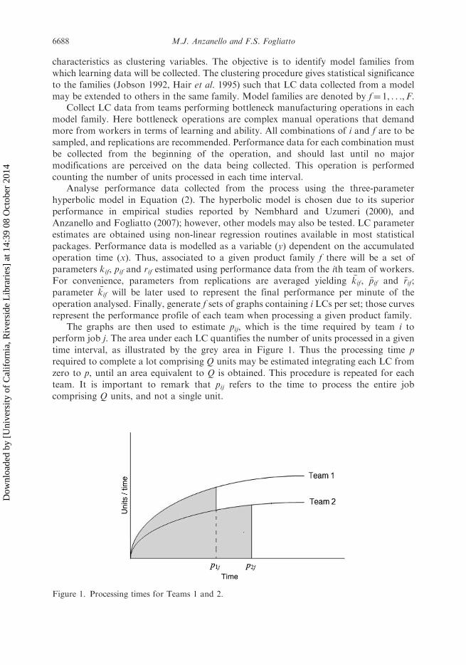
represent the performance profile of each team when processing a given product family.The graphs are then used to estimate pij, which is the time required by team i to

perform job j. The area under each LC quantifies the number of units processed in a given

time interval, as illustrated by the grey area in Figure 1. Thus the processing time p

required to complete a lot comprising Q units may be estimated integrating each LC from

zero to p, until an area equivalent to Q is obtained. This procedure is repeated for each

team. It is important to remark that pij refers to the time to process the entire job

comprising Q units, and not a single unit.

Figure 1. Processing times for Teams 1 and 2.


Dow

nloa

ded

by [

Uni

vers

ity o

f C

alif

orni

a, R

iver

side

Lib

rari

es]

at 1

4:39

08

Oct

ober

201

4

3.2 Step 2

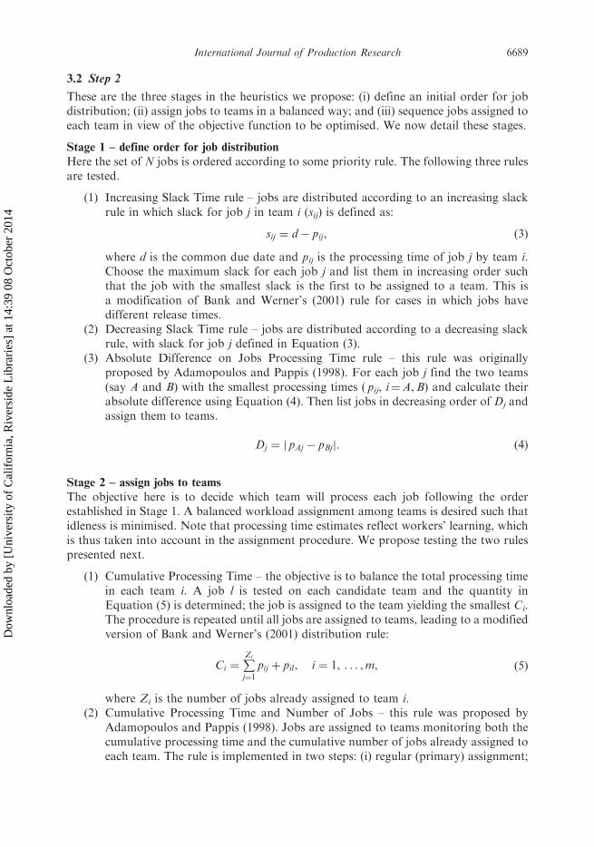
These are the three stages in the heuristics we propose: (i) define an initial order for jobdistribution; (ii) assign jobs to teams in a balanced way; and (iii) sequence jobs assigned toeach team in view of the objective function to be optimised. We now detail these stages.

Stage 1 – define order for job distribution

Here the set of N jobs is ordered according to some priority rule. The following three rulesare tested.

(1) Increasing Slack Time rule – jobs are distributed according to an increasing slackrule in which slack for job j in team i (sij) is defined as:

sij ¼ d� pij, ð3Þ

where d is the common due date and pij is the processing time of job j by team i.Choose the maximum slack for each job j and list them in increasing order suchthat the job with the smallest slack is the first to be assigned to a team. This isa modification of Bank and Werner’s (2001) rule for cases in which jobs havedifferent release times.

(2) Decreasing Slack Time rule – jobs are distributed according to a decreasing slackrule, with slack for job j defined in Equation (3).

(3) Absolute Difference on Jobs Processing Time rule – this rule was originallyproposed by Adamopoulos and Pappis (1998). For each job j find the two teams(say A and B) with the smallest processing times ( pij, i¼A,B) and calculate theirabsolute difference using Equation (4). Then list jobs in decreasing order of Dj andassign them to teams.

Dj ¼ j pAj � pBjj: ð4Þ

Stage 2 – assign jobs to teams

The objective here is to decide which team will process each job following the orderestablished in Stage 1. A balanced workload assignment among teams is desired such thatidleness is minimised. Note that processing time estimates reflect workers’ learning, whichis thus taken into account in the assignment procedure. We propose testing the two rulespresented next.

(1) Cumulative Processing Time – the objective is to balance the total processing timein each team i. A job l is tested on each candidate team and the quantity inEquation (5) is determined; the job is assigned to the team yielding the smallest Ci.The procedure is repeated until all jobs are assigned to teams, leading to a modifiedversion of Bank and Werner’s (2001) distribution rule:

Ci ¼PZi

j¼1

pij þ pil, i ¼ 1, . . . ,m, ð5Þ

where Zi is the number of jobs already assigned to team i.(2) Cumulative Processing Time and Number of Jobs – this rule was proposed by

Adamopoulos and Pappis (1998). Jobs are assigned to teams monitoring both thecumulative processing time and the cumulative number of jobs already assigned toeach team. The rule is implemented in two steps: (i) regular (primary) assignment;


Dow

nloa

ded

by [

Uni

vers

ity o

f C

alif

orni

a, R

iver

side

Lib

rari

es]

at 1

4:39

08

Oct

ober

201

4

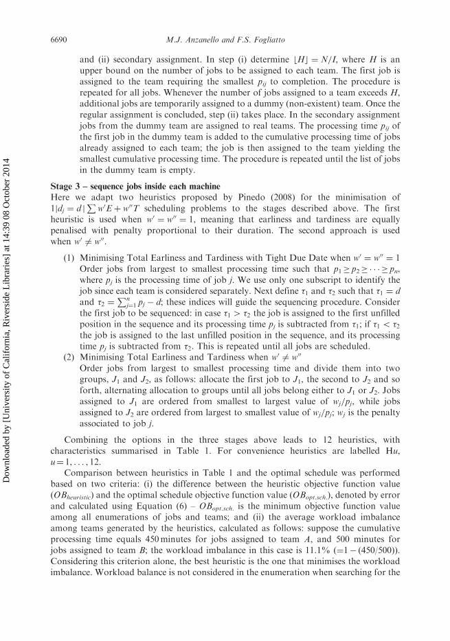
and (ii) secondary assignment. In step (i) determine Hb c ¼ N=I, where H is anupper bound on the number of jobs to be assigned to each team. The first job isassigned to the team requiring the smallest pij to completion. The procedure isrepeated for all jobs. Whenever the number of jobs assigned to a team exceeds H,additional jobs are temporarily assigned to a dummy (non-existent) team. Once theregular assignment is concluded, step (ii) takes place. In the secondary assignmentjobs from the dummy team are assigned to real teams. The processing time pij ofthe first job in the dummy team is added to the cumulative processing time of jobsalready assigned to each team; the job is then assigned to the team yielding thesmallest cumulative processing time. The procedure is repeated until the list of jobsin the dummy team is empty.

Stage 3 – sequence jobs inside each machine

Here we adapt two heuristics proposed by Pinedo (2008) for the minimisation of1jdj ¼ d j

Pw0Eþ w00T scheduling problems to the stages described above. The first

heuristic is used when w0 ¼ w00 ¼ 1, meaning that earliness and tardiness are equallypenalised with penalty proportional to their duration. The second approach is usedwhen w0 6¼ w00.

(1) Minimising Total Earliness and Tardiness with Tight Due Date when w0 ¼ w00 ¼ 1Order jobs from largest to smallest processing time such that p1� p2� � � � � pn,where pj is the processing time of job j. We use only one subscript to identify thejob since each team is considered separately. Next define �1 and �2 such that �1 ¼ dand �2 ¼

Pnj¼1 pj � d; these indices will guide the sequencing procedure. Consider

the first job to be sequenced: in case �1 4 �2 the job is assigned to the first unfilledposition in the sequence and its processing time pj is subtracted from �1; if �1 5 �2the job is assigned to the last unfilled position in the sequence, and its processingtime pj is subtracted from �2. This is repeated until all jobs are scheduled.

(2) Minimising Total Earliness and Tardiness when w0 6¼ w00

Order jobs from largest to smallest processing time and divide them into twogroups, J1 and J2, as follows: allocate the first job to J1, the second to J2 and soforth, alternating allocation to groups until all jobs belong either to J1 or J2. Jobsassigned to J1 are ordered from smallest to largest value of wj=pj, while jobsassigned to J2 are ordered from largest to smallest value of wj=pj; wj is the penaltyassociated to job j.

Combining the options in the three stages above leads to 12 heuristics, withcharacteristics summarised in Table 1. For convenience heuristics are labelled Hu,u¼ 1, . . . , 12.

Comparison between heuristics in Table 1 and the optimal schedule was performedbased on two criteria: (i) the difference between the heuristic objective function value(OBheuristic) and the optimal schedule objective function value (OBopt.sch.), denoted by errorand calculated using Equation (6) – OBopt.sch. is the minimum objective function valueamong all enumerations of jobs and teams; and (ii) the average workload imbalanceamong teams generated by the heuristics, calculated as follows: suppose the cumulativeprocessing time equals 450minutes for jobs assigned to team A, and 500 minutes forjobs assigned to team B; the workload imbalance in this case is 11.1% (¼1� (450/500)).Considering this criterion alone, the best heuristic is the one that minimises the workloadimbalance. Workload balance is not considered in the enumeration when searching for the


Dow

nloa

ded

by [

Uni

vers

ity o

f C

alif

orni

a, R

iver

side

Lib

rari

es]

at 1

4:39

08

Oct

ober

201

4

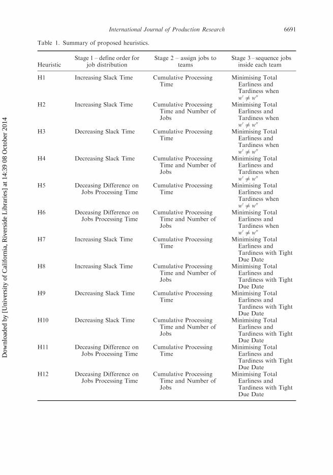
Table 1. Summary of proposed heuristics.

HeuristicStage 1 – define order for

job distributionStage 2 – assign jobs to

teamsStage 3 – sequence jobs

inside each team

H1 Increasing Slack Time Cumulative ProcessingTime

Minimising TotalEarliness andTardiness whenw0 6¼ w00

H2 Increasing Slack Time Cumulative ProcessingTime and Number ofJobs


H3 Decreasing Slack Time Cumulative ProcessingTime


H4 Decreasing Slack Time Cumulative ProcessingTime and Number ofJobs


H5 Deceasing Difference onJobs Processing Time

Cumulative ProcessingTime



Cumulative ProcessingTime and Number ofJobs


H7 Increasing Slack Time Cumulative ProcessingTime

Minimising TotalEarliness andTardiness with TightDue Date

H8 Increasing Slack Time Cumulative ProcessingTime and Number ofJobs


H9 Decreasing Slack Time Cumulative ProcessingTime


H10 Decreasing Slack Time Cumulative ProcessingTime and Number ofJobs



Cumulative ProcessingTime



Cumulative ProcessingTime and Number ofJobs



Dow

nloa

ded

by [

Uni

vers

ity o

f C

alif

orni

a, R

iver

side

Lib

rari

es]

at 1

4:39

08

Oct

ober

201

4

optimal solution; however, it is an intuitive result that the minimal objective function valuecorresponds to a job sequence that balances the workload among the teams.

error ¼OBheuristic �OBopt:sch:

OBopt:sch:: ð6Þ

4. Case example

The method was applied in a shoe manufacturing plant in the south of Brazil. Shoeproducers have faced decreasing lot sizes in the past decade, forcing their mass productionconfiguration to adapt to an increasingly customised market. Shoes are assembledfollowing a number of operations; independent of the type of shoe produced the sewingoperation is the bottleneck in the plant analysed, being highly dependent on workers’manual skills.

Twenty shoe models were considered in the study. Models were characterised withrespect to manufacturing complexity through the following clustering variables: overallcomplexity, parts complexity (deployed into four categories), number of parts in themodel, and type of shoe. The first six variables were subjectively assessed by companyexperts using a 3-point scale, where 3 denotes the highest complexity or number of parts.The variable type of shoe has two levels: 1 for shoes and sandals, and 2 for boots, whichtend to be more complex in terms of assembly. A k-means cluster analysis on the 20 modelsled to three complexity families labelled as Easy, Medium, and Difficult.

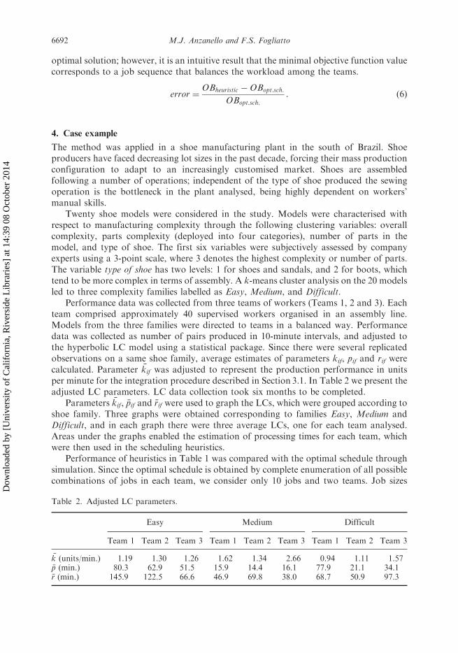
Performance data was collected from three teams of workers (Teams 1, 2 and 3). Eachteam comprised approximately 40 supervised workers organised in an assembly line.Models from the three families were directed to teams in a balanced way. Performancedata was collected as number of pairs produced in 10-minute intervals, and adjusted tothe hyperbolic LC model using a statistical package. Since there were several replicatedobservations on a same shoe family, average estimates of parameters kif, pif and rif werecalculated. Parameter �kif was adjusted to represent the production performance in unitsper minute for the integration procedure described in Section 3.1. In Table 2 we present theadjusted LC parameters. LC data collection took six months to be completed.

Parameters �kif, �pif and �rif were used to graph the LCs, which were grouped according toshoe family. Three graphs were obtained corresponding to families Easy, Medium andDifficult, and in each graph there were three average LCs, one for each team analysed.Areas under the graphs enabled the estimation of processing times for each team, whichwere then used in the scheduling heuristics.

Performance of heuristics in Table 1 was compared with the optimal schedule throughsimulation. Since the optimal schedule is obtained by complete enumeration of all possiblecombinations of jobs in each team, we consider only 10 jobs and two teams. Job sizes

Table 2. Adjusted LC parameters.

Easy Medium Difficult

Team 1 Team 2 Team 3 Team 1 Team 2 Team 3 Team 1 Team 2 Team 3

�k (units/min.) 1.19 1.30 1.26 1.62 1.34 2.66 0.94 1.11 1.57�p (min.) 80.3 62.9 51.5 15.9 14.4 16.1 77.9 21.1 34.1�r (min.) 145.9 122.5 66.6 46.9 69.8 38.0 68.7 50.9 97.3


Dow

nloa

ded

by [

Uni

vers

ity o

f C

alif

orni

a, R

iver

side

Lib

rari

es]

at 1

4:39

08

Oct

ober

201

4

(in units) were assumed to follow a N�ð�, �2Þ distribution. We tested three job sizes

frequently demanded in practice: N� (500,100), N� (300,75) and N� (150,25). A due date

d for each set of jobs was defined using expert opinion: 25 hours for a set of 10 jobs

generated using N� (500,100), 15 hours using N� (300,75), and 10 hours using

N� (150,25). In addition, each job was randomly inserted into a complexity family. For

that we used a uniform distribution on the interval [1,3], where 1 corresponds to Easy, 2 to

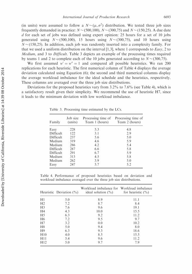
Medium, and 3 to Difficult. Table 3 depicts an example of the processing times required

by teams 1 and 2 to complete each of the 10 jobs generated according to N� (300,75).We first assumed w0 ¼ w00 ¼ 1 and compared all possible heuristics. We ran 200

replications for each heuristic. The first numerical column of Table 4 displays the average

deviation calculated using Equation (6); the second and third numerical columns display

the average workload imbalance for the ideal schedule and the heuristics, respectively.

These columns are averaged over the three job size distributions.Deviations for the proposed heuristics vary from 3.2% to 7.6% (see Table 4), which is

a satisfactory result given their simplicity. We recommend the use of heuristic H7, since

it leads to the minimum deviation with low workload imbalance.

Table 4. Performance of proposed heuristics based on deviation andworkload imbalance averaged over the three job size distributions.

Heuristic Deviation (%)Workload imbalance for

ideal solution (%)Workload imbalancefor heuristic (%)

H1 5.0 8.9 11.1H2 7.2 8.7 8.4H3 7.6 9.6 19.1H4 4.3 10.0 15.5H5 6.3 9.2 11.2H6 7.2 9.5 9.7H7 3.2 0.0 10.2H8 5.0 9.4 8.0H9 6.3 9.3 18.6H10 4.0 8.5 15.5H11 5.4 9.6 11.2H12 5.0 9.7 7.9

Table 3. Processing time estimated by the LCs.

FamilyJob size(units)

Processing time ofTeam 1 (hours)

Processing time ofTeam 2 (hours)

Easy 228 5.3 4.8Difficult 122 3.1 2.9Difficult 237 5.6 5.0Medium 319 4.6 5.9Medium 286 4.2 5.4Difficult 287 6.6 5.8Difficult 291 6.7 5.9Medium 313 4.5 5.8Medium 262 3.9 5.0Easy 247 5.7 5.2


Dow

nloa

ded

by [

Uni

vers

ity o

f C

alif

orni

a, R

iver

side

Lib

rari

es]

at 1

4:39

08

Oct

ober

201

4

Additionally, we conduct a performance analysis on each stage of the heuristics. Values

for one stage are based on the average of the other two, e.g., performance of rules for Stage 1

was averaged over Stages 2 and 3. As depicted in Table 5, the Increasing Slack Time rule

is the best with respect to deviation and workload imbalance when Stage 1 is considered.

For Stage 2, the rules tested are equivalent in terms of deviation, but we recommend

the Cumulative Processing Time due to its simplicity (see Table 6). The algorithm for

Minimising Total Earliness and Tardiness with Tight Due Date is the best option for

Stage 3, since it leads to significantly smaller deviation (see Table 7).There are no significant differences or perceptible trends in the heuristics’ performance

as a function of job size, as depicted in Table 8. Heuristic H7 performs consistently better

for all job size distributions considered in the simulation.Simulations considering w0 6¼ w00 were performed using all rules of Stages 1 and 2, but

only the algorithm for Minimising Total Earliness and Tardiness when w0 6¼ w00 in Stage 3

(corresponding to heuristics H1 to H6 in Table 1). Weights w0 and w00 were randomly

generated using a uniform distribution on the interval [1,3]. Table 9 displays slightly higher

deviations than those observed when weights were all set to 1. When w0 6¼ w00, H2 is the

recommended heuristic since it provides a better compromise of percentage deviation and

workload imbalance among teams. Note that the workload imbalance generated by the

Table 7. Performance of algorithms for Stage 3 (averaged over Stages 1 and 2).

Algorithms for Stage 3 Deviation (%)Wordload imbalance for

ideal solution (%)Wordload imbalancefor heuristic (%)

Minimising Total Earlinessand Tardiness whenw0 6¼ w00

6.3 9.5 12.2

Minimising Total Earlinessand Tardiness with TightDue Date

4.8 9.2 12.1

Table 5. Performance of rules for Stage 1 (averaged over Stages 2 and 3).

Rules for Stage 1 Deviation (%)Wordload imbalance for


Increasing Slack Time 5.1 9.0 9.4Decreasing Slack Time 5.5 9.3 17.2Decreasing Difference on

Jobs Processing Times6.0 9.5 10.0

Table 6. Performance of rules for Stage 2 (averaged over Stages 1 and 3).

Rules for Stage 2 Deviation (%)Wordload imbalance for


Cumulative Processing Time 5.6 9.4 13.7Cumulative Processing Time

and Number of Jobs5.4 9.4 10.5


Dow

nloa

ded

by [

Uni

vers

ity o

f C

alif

orni

a, R

iver

side

Lib

rari

es]

at 1

4:39

08

Oct

ober

201

4

heuristic can be smaller than that obtained in the optimal solution, since the optimal

solution is objective function driven.We then apply heuristic H7 to a shoe manufacturing scenario consisting of 110 jobs

and three teams. The situation where w0 ¼ w00 ¼ 1 is adequate for this case, according to

company experts. The Appendix depicts job sizes and complexity; d is set to 200 hours in

this analysis. Here we decided to measure the workload in terms of busy time rather than

imbalance, since it is more intuitive when more than two teams are considered. Table 10

Table 8. Deviations under different job size distributions.

Heuristic

Job size distribution (in units)

N� (500,100) N� (300,75) N� (150,25)

H1 4.6 4.9 5.5H2 6.7 6.1 8.8H3 6.9 8.9 7.1H4 3.6 3.2 5.9H5 5.5 6.3 7.0H6 6.3 7.0 8.4H7 3.6 3.4 2.7H8 6.0 4.6 4.4H9 7.5 6.5 4.9H10 4.3 4.5 3.3H11 5.4 5.9 4.9H12 5.1 3.9 5.9

Table 9. Performance of proposed heuristics when w0 6¼ w00.

Heuristic Deviation (%)Workload imbalance for

ideal solution (%)Workload imbalancefor heuristic (%)

H1 11.3 10.6 11.6H2 11.3 10.3 7.4H3 14.7 11.3 17.9H4 11.1 10.8 13.3H5 13.6 10.4 11.7H6 12.2 10.6 7.7

Table 10. Job sequence and busy time for the shoe manufacturing scenario.

Team Job order (identified by ID) Busy time (%)

Team 1 93 77 109 61 52 41 75 60 54 68 40 22 108 102 56 16 92 2 91 80 33 49 123 70 10 32 45 24 63 4 64

100

Team 2 89 50 67 15 105 30 88 35 6 94 62 21 65 101 76 8 81 11 106 17 5 85 7186 55 34 19 23 46 84 48 26 69 110

99.3

Team 3 97 72 18 79 37 47 7 73 100 59 82 95 103 44 83 90 9 43 38 31 107 27 7887 25 1 99 28 96 57 39 14 36 98 51 58 29 74 42 53 20 13 66 104

99.9


Dow

nloa

ded

by [

Uni

vers

ity o

f C

alif

orni

a, R

iver

side

Lib

rari

es]

at 1

4:39

08

Oct

ober

201

4

displays the job scheduling and percentage of busy time for each team. More jobs areassigned to Team 3 due to its higher final performance and faster learning rate, expressedby parameters k and r, respectively, in Table 2. In addition, the recommended heuristicleads to a remarkable balance between teams’ busy times.

5. Conclusion

We proposed a method to schedule jobs in highly customised applications where workers’learning takes place. The method integrates learning curves to new scheduling heuristicsaimed at minimising the total weighted earliness and tardiness. Learning curves enabledestimating the processing time required by teams of workers to complete jobs of differentsize and complexity. Such times were used in 12 heuristics created by combining availableheuristics for the unrelated parallel machine problem. The best heuristic determined basedon a simulation study yielded an average deviance of 3.2% compared to the optimalschedule, and led to satisfactory workload balance among teams. When applied to a shoemanufacturing case study the recommended heuristic prioritised job allocation to thefastest team and led to remarkable workload balance among teams.

We now present some future research directions using the developments in this paperas a starting point. The first relates to the prediction error associated with LC modelling.Estimates of job completion times are affected by the LC goodness-of-fit, as reportedby Finch and Luebbe (1991, 1995). Imprecise estimates from LCs lead to unreliablescheduling results, particularly when the time to complete a batch of jobs is considered.LC goodness-of-fit may be assessed by the model’s coefficient of determination, R2. Weenvision the use of these coefficients to reorganise jobs in the scheduling procedure suchthat those with early due dates and completion times obtained from LCs with high R2

coefficients are prioritised.Imprecision in LC estimates motivates our second envisioned future research issue.

We would like to investigate multivariate LC models that take into account theeffect of other independent variables, in addition to time (see Badiru 1992, for anintroduction on multivariate LCs). One such variable could be different varieties oftraining procedures.

The third future research deployment deals with the analysis of more complexscheduling problems where workers’ learning takes place, such as pure mass customisedjob shop environments. In those production systems LC modelling becomes quitechallenging due to the high variety of products involved and their small lot sizes. Theplanning and optimisation of LC data collection in environments of potential data scarcitysuch as these is a key research problem.

References

Adamopoulos, G. and Pappis, C., 1998. Scheduling under a common due-date on parallel unrelated

machines. European Journal of Operational Research, 105 (3), 494–501.

Anzanello, M. and Fogliatto, F., 2007. Learning curve modeling of work assignment in

mass customized assembly lines. International Journal of Production Research, 45 (13),

2919–2938.Badiru, A., 1992. Computational survey of univariate and multivariate learning curve models.

IEEE Transactions on Engineering Management, 39 (2), 176–188.


Dow

nloa

ded

by [

Uni

vers

ity o

f C

alif

orni

a, R

iver

side

Lib

rari

es]

at 1

4:39

08

Oct

ober

201

4

Bank, J. and Werner, F., 2001. Heuristic algorithms for unrelated parallel machine scheduling witha common due date, release dates, and linear earliness and tardiness penalties. Mathematicaland Computer Modelling, 33 (4), 363–383.

Biskup, D., 1999. Single-machine scheduling with learning considerations. European Journal of

Operational Research, 115 (1), 173–178.Cheng, T. and Sin C., 1990. A state-of-the-art review of parallel-machine scheduling research.

European Journal of Operational Research, 47 (33), 271–292.

Chen, J. and Wu, T., 2006. Total tardiness minimization on unrelated parallel machine schedulingwith auxiliary equipment constraints. Omega, 34 (1), 81–89.

Da Silveira, G., Borestein, D., and Fogliatto, F., 2001. Mass customization: literature review and

research direction. International Journal of Production Economics, 72 (1), 1–13.Finch, B. and Luebbe, R., 1991. Risk associated with learning curve estimates. Production and

Inventory Management Journal, 32 (1), 73–76.

Finch, B. and Luebbe, R., 1995. The impact of learning rate and constraints on system performance.International Journal of Production Research, 33 (3), 631–642.

Jobson, J., 1992. Applied Multivariate Data Analysis, Volume II: Categorical and MultivariateMethods. New York: Springer-Verlag.

Kientzle, M., 1946. Properties of learning curves under varied distributions of practice. Journal ofExperimental Psychology, 36 (1), 187–211.

Hair, J.F., et al., 1995. Multivariate data analysis with readings. Englewood Cliffs, NJ: Prentice-Hall.

Leonardi, S. and Raz, D., 2007. Approximating total flow time on parallel machines. Journal ofComputer and System Sciences, 73 (6), 875–891.

Mattfeld, D. and Bierwirth, C., 2004. An efficient genetic algorithm for job shop scheduling with

tardiness objectives. European Journal of Operations Research, 155 (3), 616–630.Mokotoff, E. and Jimeno, J., 2002. Heuristics based on partial enumeration for the

unrelated parallel processor scheduling problem. Annals of Operations Research, 117 (1–4),133–150.

Mosheiov, G., 2001a. Scheduling problems with learning effect. European Journal of OperationalResearch, 132 (3), 687–693.

Mosheiov, G., 2001b. Parallel machine scheduling with learning effect. Journal of the Operational

Research Society, 52 (1), 391–399.Mosheiov, G. and Sidney, J., 2003. Scheduling with general job-dependent learning curves. European

Journal of Operational Research, 147 (3), 665–670.

Nembhard, D.A. and Uzumeri, M.V., 2000. An individual-based description of learning withinan organization. IEEE Transactions on Engineering Management, 47 (3), 370–378.

Pinedo, M., 2008. Scheduling, theory, algorithms and systems. New York: Springer.

Randahwa, S. and Kuo, C., 1997. Evaluating scheduling heuristics for non-identical parallelprocessors. International Journal of Production Research, 35 (4), 969–981.

Suresh, V. and Chaudhuri, D., 1994. Minimizing maximum tardiness for unrelated parallelmachines. International Journal of Production Economics, 34 (22), 223–229.

Teplitz, C.J., 1991. The learning curve deskbook: a reference guide to theory, calculations andapplications. New York: Quorum Books.

Thurstone, L., 1919. The Learning curve equation. California: Psychological Review Company.

Uzumeri, M. and Nembhard, D., 1998. A population of learners: a new way to measureorganizational learning. Journal of Operations Management, 16 (5), 515–528.

Wright, T., 1936. Factors affecting the cost of airplanes. Journal of the Aeronautical Sciences, 3 (1),

122–128.Yu, L, et al., 2002. Scheduling of unrelated parallel machines: an application to PWB

manufacturing. IIE Transactions, 34 (11), 921–931.


Dow

nloa

ded

by [

Uni

vers

ity o

f C

alif

orni

a, R

iver

side

Lib

rari

es]

at 1

4:39

08

Oct

ober

201

4

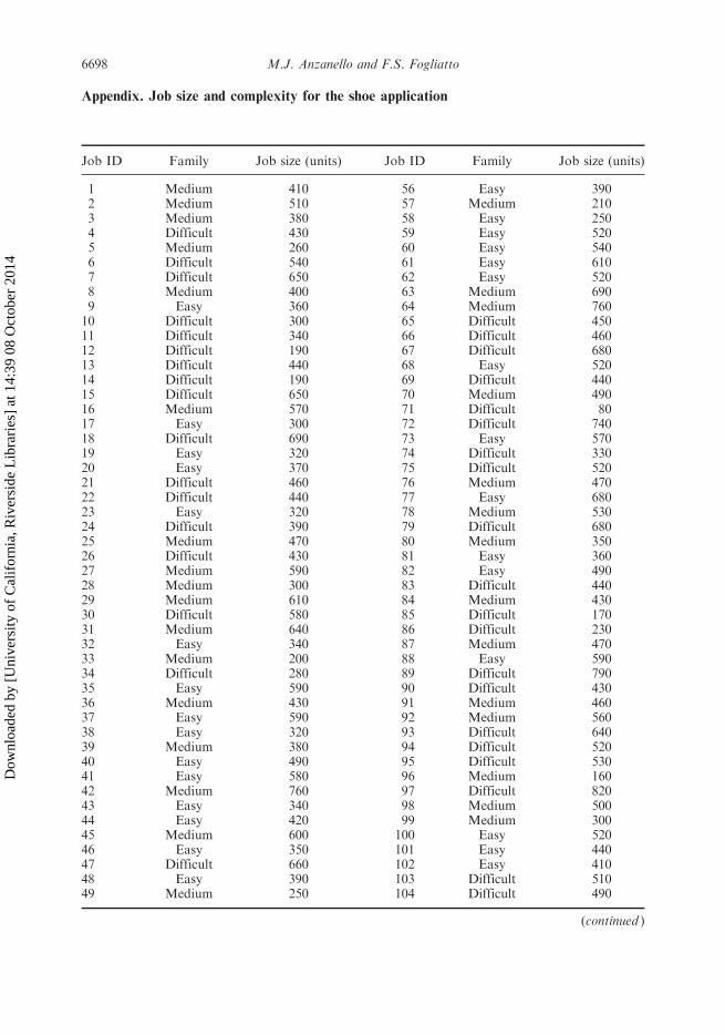
Appendix. Job size and complexity for the shoe application

Job ID Family Job size (units) Job ID Family Job size (units)

1 Medium 410 56 Easy 3902 Medium 510 57 Medium 2103 Medium 380 58 Easy 2504 Difficult 430 59 Easy 5205 Medium 260 60 Easy 5406 Difficult 540 61 Easy 6107 Difficult 650 62 Easy 5208 Medium 400 63 Medium 6909 Easy 360 64 Medium 76010 Difficult 300 65 Difficult 45011 Difficult 340 66 Difficult 46012 Difficult 190 67 Difficult 68013 Difficult 440 68 Easy 52014 Difficult 190 69 Difficult 44015 Difficult 650 70 Medium 49016 Medium 570 71 Difficult 8017 Easy 300 72 Difficult 74018 Difficult 690 73 Easy 57019 Easy 320 74 Difficult 33020 Easy 370 75 Difficult 52021 Difficult 460 76 Medium 47022 Difficult 440 77 Easy 68023 Easy 320 78 Medium 53024 Difficult 390 79 Difficult 68025 Medium 470 80 Medium 35026 Difficult 430 81 Easy 36027 Medium 590 82 Easy 49028 Medium 300 83 Difficult 44029 Medium 610 84 Medium 43030 Difficult 580 85 Difficult 17031 Medium 640 86 Difficult 23032 Easy 340 87 Medium 47033 Medium 200 88 Easy 59034 Difficult 280 89 Difficult 79035 Easy 590 90 Difficult 43036 Medium 430 91 Medium 46037 Easy 590 92 Medium 56038 Easy 320 93 Difficult 64039 Medium 380 94 Difficult 52040 Easy 490 95 Difficult 53041 Easy 580 96 Medium 16042 Medium 760 97 Difficult 82043 Easy 340 98 Medium 50044 Easy 420 99 Medium 30045 Medium 600 100 Easy 52046 Easy 350 101 Easy 44047 Difficult 660 102 Easy 41048 Easy 390 103 Difficult 51049 Medium 250 104 Difficult 490

(continued )


Dow

nloa

ded

by [

Uni

vers

ity o

f C

alif

orni

a, R

iver

side

Lib

rari

es]

at 1

4:39

08

Oct

ober

201

4

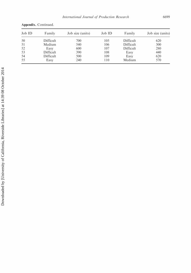
Appendix. Continued.

Job ID Family Job size (units) Job ID Family Job size (units)

50 Difficult 700 105 Difficult 62051 Medium 540 106 Difficult 30052 Easy 600 107 Difficult 28053 Difficult 390 108 Easy 44054 Difficult 500 109 Easy 62055 Easy 240 110 Medium 570


Dow

nloa

ded

by [

Uni

vers

ity o

f C

alif

orni

a, R

iver

side

Lib

rari

es]

at 1

4:39

08

Oct

ober

201

4

Documents

Scheduling learning dependent jobs in customised assembly lines