Embed Size (px)
Citation preview

UNIVERSITY OF POTSDAM
Institute of Physics and AstronomyAPPLIED CONDENSED MATTER PHYSICS
P H D – T H E S I S
Scattering Effects in the Sound
Wave Propagation of Instrument
Soundboards
Presented by
Marcel Kappel
Thesis Supervisor: Prof. Dr.-Ing. Reimund Gerhard
Second Supervisor: Prof. Dr. rer. nat. Markus Abel

This work is licensed under a Creative Commons License: Attribution - Noncommercial - Share Alike 3.0 Germany To view a copy of this license visit http://creativecommons.org/licenses/by-nc-sa/3.0/de/ Published online at the Institutional Repository of the University of Potsdam: URL http://opus.kobv.de/ubp/volltexte/2012/6267/ URN urn:nbn:de:kobv:517-opus-62676 http://nbn-resolving.de/urn:nbn:de:kobv:517-opus-62676

Die Normalität ist eine gepflasterte Straße;
man kann gut darauf laufen,
doch es wachsen keine Blumen auf ihr.
(Vincent van Gogh)


Acknowledgments
Firstly, I would like to express my thanks to everyone who supported meduring my PhD time.
Most of all I want to thank my supervisor Prof. Dr. ReimundGerhard for the great opportunity to write my PhD thesis at the AppliedCondensed-Matter Physics (ACMP) group and all the support he gave meduring my work. Also I want to thank my advisor Prof. Dr. Markus Abelas he always took the time for me, even if he had no time due to his variousother duties.I am truly indebted to the piano manufacturer ’C. Bechstein Pianofortefabrik’for the opportunity to perfom measurements on one of their upright pianos.In particular, I would like to give special thanks to Werner Albrecht, forgiving me a lot of his attention and time during these measurements.I also thank Michael Winkler and Jost Fischer for the good teamworkregarding the Schuke project.Many thanks to the people from the ACMP, who increased my understanding,by valuable talks and discussions during the last three years, not only inpolymer physics but also in acoustics. In particular, I thank Gunnar, René,Matthias, Lars, Werner, Alex and Peter for all the great support they gave meand I apologize for the time they spent with me to discuss various problems.Also many thanks to Steffen, Marc, Mareike, Daniel, André, Peter, Lena,Sebastian, Alena, Nika for enriching my life with their friendship. My deepestthanks and respect go to Matthias and Andreas who have been good friendsall the time at the university.
Finally, I want to thank and acknowledge my parents and my brother fortheir support by any means. Without their help I would not have been whereI am now.
... many, many thanks to Konstanze for everything ...


Abstract
In the western hemisphere, the piano is one of the most important instruments.While its evolution lasted for more than three centuries, and the mostimportant physical aspects have already been investigated, some parts in thecharacterization of the piano remain not well understood. Considering thepivotal piano soundboard, the effect of ribs mounted on the board exertedon the sound radiation and propagation in particular, is mostly neglegted inthe literature. The present investigation deals exactly with the sound wavepropagation effects that emerge in the presence of an array of equally-distantmounted ribs at a soundboard. Solid-state theory [Ziman 1972, Ashcroft 1976]proposes particular eigenmodes and -frequencies for such arrangements, whichare comparable to single units in a crystal. Following this ’linear chain model’(LCM), differences in the frequency spectrum are observable as a distinct bandstructure. Also, the amplitudes of the modes are changed, due to differencesof the damping factor.
These scattering effects were not only investigated for a well-understoodconceptional rectangular soundboard (multichord), but also for a genuinepiano resonance board manufactured by the piano maker company ’C.Bechstein Pianofortefabrik’. To obtain the possibility to distinguish betweenthe characterizing spectra both with and without mounted ribs, the typicalassembly plan for the Bechstein instrument was specially customized. Spectralsimilarities and differences between both boards are found in terms of dampingand tone.
Furthermore, specially prepared minimal-invasive piezoelectric polymersensors made from polyvinylidene fluoride (PVDF) [Kappel 2011] were usedto record solid-state vibrations of the investigated system. The essentialcalibration and characterization of these polymer sensors was performedby determining the electromechanical conversion, which is represented bythe piezoelectric coefficient d33. Therefore, the robust ’sinusoidally varyingexternal force’ method [Altafim 2009, Kressmann 2001] was applied, where adynamic force perpendicular to the sensor’s surface, generates movable chargecharriers. Crucial parameters were monitored, with the frequency responsefunction as the most important one for acousticians.
Along with conventional condenser microphones, the sound was measuredas solid-state vibration as well as airborne wave. On this basis, statementscan be made about emergence, propagation, and also the overall radiation

iv Chapter 0. Abstract
of the generated modes of the vibrating system. Ultimately, these resultsacoustically characterize the entire system.
Deutsche Zusammenfassung
Betrachtet man den westlichen Kulturkreis, ist der Flügel bzw. das Klavierwohl eines der bedeutendsten Instrumente. Trotz einer stetigen, empirischenWeiterentwicklung dieses Instrumentes in den letzten drei Jahrhunderten unddes Wissens um die wichtigsten physikalischen Effekte, sind viele Teile derCharakterisierung des Klaviers (sowohl akustisch als auch physikalisch) immernoch nicht vollständig verstanden. Nehmen wir nur den Resonanzboden – das
entscheidende Bauteil für die Akustik eines Klaviers – und betrachten dieAuswirkung, den die Berippung auf die Schallausbreitung des Instrumentshat. Bis auf wenige Ausnahmen ([Wogram 1980, Giordano 1997]) wirddieser Struktur-Aspekt in der Literatur weitestgehend übergangen. Dievorliegende Arbeit untersucht genau diese Ausbreitungscharakteristiken undStreueffekte, welche dadurch entstehen, dass Rippen, die denselben Abstandzueinander haben, auf dem Resonanzboden angebracht werden. DieFestkörperphysik stellt ein einfaches Modell ([Ziman 1972, Ashcroft 1976])über die Eigenfrequenzen für solche Anordnungen bereit. Dafür werden dieRippen und deren Abstände wie Einheitszellen eines Kristalls betrachtet.Ausgehend vom sogenannten ’Modell der linearen Ketten’, werden gemesseneFrequenzbänder im Spektrum erklärbar. Zusätzlich ändern sich auch diespektralen Amplituden des Resonanzbodens durch das Anbringen der Rippen.
Diese Streueffekte wurden nicht nur an einem konzeptionellenrechteckigen Resonanzboden untersucht, sondern auch an einem originalenKlavier-Resonanzboden, welcher von dem Klavierbauer ’C. BechsteinPianofortefabrik’ hergestellt wurde und auch später in einem fertigen Klavierzum Einsatz kommen wird. Der traditionelle Zusammenbau des Klavierswurde speziell für diese Untersuchung abgeändert, um die Möglichkeit zuhaben, die Berippung des Resonanzbodens spektral zu charakterisieren. Allegefundenen Eigenschaften des konzeptionellen und des originalen Bodenswurden verglichen. Für die Dämpfung und für die Brillianz des Tons wurdenÜbereinstimmungen, aber auch Unterschiede gefunden.
Ein großer Teil dieser Untersuchung erforderte den Einsatz vonspeziell angefertigten piezoelektrischen Polymer-Beschleunigungsaufnehmernaus Polyvinylidenfluorid [Kawai 1969]. Direkt fest eingeklebt imInstrument, wurden diese eingesetzt, um die Körperschwingungen desvibrierenden Systems aufzunehmen [Kappel 2011]. Die essentielleKalibrierung und Charakterisierung dieser Sensoren wurde durchgeführt,

vi Chapter 0. Deutsche Zusammenfassung
indem die elektromechanische Umwandlung bestimmt wurde, die durch denpiezoelektrischen Koeffizienten d33 gegeben ist. Durch eine sinusförmigvariierende, externe Kraft und die dadurch entstehenden Ladungsträgeran den Oberflächen des Sensormaterials kann d33 sehr genau bestimmtwerden. In Abhängigkeit entscheidender physikalischer Größen, z.B. derFrequenz-Antwort-Funktion, wurde das Verhalten des piezoelektrischenKoeffizienten untersucht.
Die erzeugten Vibrationen als Körperschall (aufgenommen durch diePiezopolymere) und als Luftschallwelle (aufgenommen durch konventionelleKondensator-Mikrophone) wurden simultan gemessen und dann untersucht.Daraus kann man Aussagen über Entstehung, Ausbreitung und Abstrahlungder erzeugten Moden in das umgebende Medium ableiten. Letztlichcharakterisieren diese Ergebnisse das gesamte vibrierende System akustisch.

Contents
Acknowledgments i
Abstract iii
Deutsche Zusammenfassung v
1 Introduction 1
2 Background 5
2.1 The Piano . . . . . . . . . . . . . . . . . . . . . . . . . . . . . 52.1.1 Short History of Evolution . . . . . . . . . . . . . . . . 52.1.2 General Functioning . . . . . . . . . . . . . . . . . . . 72.1.3 Soundboard and Ribs . . . . . . . . . . . . . . . . . . . 92.1.4 Scattering generated by the Ribs . . . . . . . . . . . . 13
2.2 Piezoelectric Polymer Sensors . . . . . . . . . . . . . . . . . . 162.2.1 Piezoelectricity . . . . . . . . . . . . . . . . . . . . . . 172.2.2 Material: Why Polyvinylidene Fluoride? . . . . . . . . 182.2.3 PVDF Morphology & Piezoelectricity . . . . . . . . . . 19
3 Measurement Techniques 23
3.1 Characterization of the Measurement Room . . . . . . . . . . 233.1.1 Geometry & Material . . . . . . . . . . . . . . . . . . . 243.1.2 Sound Wave Absorption . . . . . . . . . . . . . . . . . 253.1.3 Reverberation Time . . . . . . . . . . . . . . . . . . . . 28
3.2 Preparation of the Polymer Sensors . . . . . . . . . . . . . . . 313.2.1 Sensor Production . . . . . . . . . . . . . . . . . . . . 313.2.2 Calibration & Characterization . . . . . . . . . . . . . 343.2.3 External Dynamic Force . . . . . . . . . . . . . . . . . 44
3.3 Condenser Microphones . . . . . . . . . . . . . . . . . . . . . 453.4 Chapter Conclusion . . . . . . . . . . . . . . . . . . . . . . . . 45
4 Multichord as a Conceptional Soundboard 47
4.1 LCM Model Projection to the Ribbed Soundboard . . . . . . . 474.2 Construction & Experimental Setup . . . . . . . . . . . . . . . 504.3 Rib Scattering . . . . . . . . . . . . . . . . . . . . . . . . . . . 53
4.3.1 Results . . . . . . . . . . . . . . . . . . . . . . . . . . . 534.3.2 Frequency-dependent Damping Factor . . . . . . . . . 604.3.3 Comparison: Scattering Model vs. Experimental Data 62

viii Contents
4.4 Chapter Conclusion . . . . . . . . . . . . . . . . . . . . . . . . 66
5 The Real Piano: Bechstein ’Zimmermann Z.3/116’ 69
5.1 Piano Assembly . . . . . . . . . . . . . . . . . . . . . . . . . . 695.2 Mounting the Polymer Sensors . . . . . . . . . . . . . . . . . . 715.3 Results . . . . . . . . . . . . . . . . . . . . . . . . . . . . . . . 73
5.3.1 Pulse Amplitude . . . . . . . . . . . . . . . . . . . . . 765.3.2 Normalized Spectra . . . . . . . . . . . . . . . . . . . . 785.3.3 Damping Factor . . . . . . . . . . . . . . . . . . . . . . 80
5.4 Chapter Conclusion . . . . . . . . . . . . . . . . . . . . . . . . 83
6 Conclusion and Outlook 85
A Appendix 89
A.1 Technical Background . . . . . . . . . . . . . . . . . . . . . . 89A.1.1 Microphones . . . . . . . . . . . . . . . . . . . . . . . . 89A.1.2 Acoustic Laboratory and Ambient Noise . . . . . . . . 91
A.2 Additional Theoretical Background . . . . . . . . . . . . . . . 92A.2.1 Levenberg-Marquardt Method . . . . . . . . . . . . . . 92A.2.2 Correlation Function . . . . . . . . . . . . . . . . . . . 93A.2.3 Fourier Transform . . . . . . . . . . . . . . . . . . . . . 93A.2.4 Tone Generation by a String . . . . . . . . . . . . . . . 95A.2.5 Propagation of Sound Waves in Gases . . . . . . . . . . 96A.2.6 Resonance Spectrum . . . . . . . . . . . . . . . . . . . 97A.2.7 Signal-to-Noise Ratio . . . . . . . . . . . . . . . . . . . 97A.2.8 Acoustic Dipole Radiation . . . . . . . . . . . . . . . . 98A.2.9 Impedance . . . . . . . . . . . . . . . . . . . . . . . . . 98A.2.10 Sound Pressure Quantity . . . . . . . . . . . . . . . . . 100
B Curriculum Vitæ 101
Bibliography 105
Selbstständigkeitserklärung 117

Chapter 1
Introduction
’Gravicembalo col piano e forte’, translated from Italian as ’soft and loudharpsichord’, is the original name of the piano, which is one of the mostrelevant western instruments today [Fletcher 1993]. Its functioning andcharacteristics were investigated and theoretically understood to a reasonablelevel. However, tonal differences between manufacturers and even betweensame types exist [Conklin Jr. 1996c], which are hard to explain. Regardingthe physical aspects of the instrument, many details and effects remainpoorly understood. From the perspective of sound wave radiation, the mostdelicate part of the instrument is certainly its ’loudspeaker’ – the resonanceboard or rather the soundboard1 [Wogram 1980, Giordano 1997]. But whyis it necessary to include such a board, when there are already vibratingpiano strings? The strings are not able to radiate a loud airborne soundwave directly by themselves. A larger object – the soundboard – is neededfor an efficient sound radiation. The vibrational energy generated by thestrings is transferred through the piano bridge into the soundboard, whichis, compared to piano strings, much more efficient in the airborne soundradiation2 [Suzuki 1986, Giordano 1998a, Conklin Jr. 1990].
Apart from pianos, the sound radiation of surfaces and the sound wavepropagation within a material are important to a wider class of instruments.They are also among the most important research issues considering theacoustics, because almost every stringed instrument follows the same processin the generation of a sound tone. The string vibrations are transmittedthrough a bridge to a vibrational amplification structure. Ever sincethe inauguration of stringed instruments, uncountable modifications frominstrument makers evolved these radiation bodies to the very special formsthat we know today. There are basically two amplification principles: eitherthe radiation structure exhibits a particulary complicated setup where thewhole instrument is part of the amplification surface, which is the case forviolins and guitars [Bissinger 2008, Gren 2006]. Or only few parts of the
1Both terms will be used as synonyms throughout this study.2Due to the high difference between the mass of the strings and the soundboard, which
is marked by a large mismatch of their respective impedances, the vibration is ’trapped’
within the string and is slowly leaking into the soundboard [Wogram 1980]. In detail, this
will be explained later.

2 Chapter 1. Introduction
instrument will contribute to that, which is the case for pianos. Consideringthe latter type, a specially shaped and flat resonance board amplifies the stringvibrations. In most cases, ribs are attached to the instrument soundboard.The ribs of the piano construction will have a dual function. On the one hand,they enhance the mechanical stability of the soundboard. On the other hand,they prestress the board and thus act as an energy reservoir ready to release.Although some studies on the ribs and their radiation effects have been carriedout in the past (e.g. [Wogram 1980, Giordano 1997]), the physical impact ofthis specific mechanical construction on sound radiation and propagation hasmainly been neglected in the literature.
The present investigation deals with these soundboards, their spectralradiation, and the propagation of the generated sound waves. In particular,the scattering effects originating from the ribs are studied. It is well-knownthat regular arrays of scattering obstacles, which are comparable to singleunits in a crystal, result in a band structure in the frequency spectrum(see section 2.1.4). Solid state theory [Ziman 1972, Ashcroft 1976] proposeseigenmodes and -frequencies for such arrangements. Actually only havingcoupled ocillators will also yield these band structures [Goldstein 1980].The individual scatterers for the soundboard construction are the ribs andthe board itself, featuring different cross sections (due to the ribs andother mountings), will represent the soundwave path. Given the scatteringcharacteristics of the soundboard (or crystal), the ’passing’ frequencies willarrange each other in a recognizable band structure in the frequency spectrum.
But investigation of these special effects is difficult, when the particularlyshaped resonance board of a piano is considered: the emerging eigenmodesheavily depend on the specific shape. Nevertheless, a theoretical configurationof a surface structured with ribs in a regular array, can be mapped to the realsoundboard. Under mild restrictions, the frequency spectrum between theoryand experiment will be similar. Consequently, it was decided to additionallybuild rectangular conceptual soundboard [Kappel 2010] as a dedicated setup,which topologically mimicks a piano soundboard. It is easily understood,cheap, and well controllable. The impact of the mounted ribs on theradiated spectrum of a multichord (chapter 4) and on a real piano soundboardmanufactured by Bechstein (chapter 5) is systematically studied. Regardingthe measurements on the real Bechstein soundboard, the traditional assemblysequence of the piano was customized3. Similarities and differences betweenboth boards (multichord and Bechstein soundboard) will be represented in
3Usually, the bridge and the ribs of the piano are mounted onto the soundboard at once.
In order to distinguish between the characteristic spectra both with and without mounted
ribs, this step was subdivided.

3
terms of damping and tone.At this point, the question arises, what is the best way to measure the
sound wave propagation and the scattering effects? To distinguish betweenradiated airborne sound and sound waves propagated inside the board,piezoelectric accelerometers were used throughout this investigation. Thesespecially prepared solid-state vibrational sensors represent a class of innovativeand minimal-invasive recording sensors, which are also highly flexible andrelatively inexpensive. The complete preparation and the characterizationprocess of these measurement devices are documented and discussed (seeSec. 3.2 and [Kappel 2011]). Under external force, the calibration of thepolymer relaxation was of major concern over short and long term scales.The main procedure utilized for the probe characterization and calibrationis the determination of the piezoelectric coefficient d33 as described by[Altafim 2009, Kressmann 2001] and also in Sec. 3.2. From the perspective ofvibrational measurements, the most important parameters from the inside ofa setup were monitored, namely the static force, the amplitude of the dynamicforce, the frequency response, and the long-term stability. Moreover, it willbe shown in this study that it is possible to compensate these effects of theparameter drift resulting from external stress.
Additionally, a new acoustic recording procedure will be presented. Itis a result of the combination of measurements of solid-state vibrations(piezoelectric polymer) and radiated airborne sound (conventional condensermicrophones). Both data acquisitions will be performed simultaneously. Thisprocedure can be recommended as an optimal method for investigation ofthe temporal distribution of vibrational energy in a system to be measured.
The presented thesis consists of three main parts:
• The detailed description of the piano tone generating mechanism as wellas the commonly used theory of piano physics is summarized in the firstchapter. Furthermore, the ’linear chain model’ (LCM), a ’mass-spring’scattering model, is provided from the solid state physics explaining therib influence on sound wave propagation.
• In the second chapter the measurements of the room characteristics ofthe recording room in which the multichord measurements had takenplace are provided. Also, the detailed preparation, calibration, andcharacterization of the piezoelectric polymer devices are given here.
• The main part of the study will be presented in chapters 4 and 5,which finally explain the investigations performed at the conceptualsoundboard and the Bechstein upright piano ’Z.3/116’ soundboard.

4 Chapter 1. Introduction
The obtained results, spectral differences and similarities as well as thecomparison to the LCM are presented and discussed in these chapters.
The thesis concludes with the summary and outlook.

Chapter 2
Background
In section 2.1 the piano evolution, the mechanical sequence of the tonegeneration and the underlying physics are introduced. Different pianomanufacturers produce different instruments, which can result in missingbrilliance or increased sound radiation for certain frequencies. Thesedifferences may be attributed to the geometry and restrictions in theconstruction of the soundboard which acts as the last acoustical filter beforethe sound is radiated towards the audience listening. Because it is one of themajor investigation part of the thesis, the role of the soundboard and the ribsfor the sound wave propagation of the piano is highlighted in particular. Amodel (see Sec. 2.1.4) proposed by solid-state-physics, the ’linear chain model’(LCM), can be applied for the frequency radiation and propagation patternof the soundboard, dependent on the mounted ribs of the resonance board.
Since it is used as sensor material throughout this investigation, thesecond part of this chapter describes the morphology and related materialproperties of polyvinylindene fluoride (PVDF). For the understanding ofthe piezoelectricity of PVDF it is important to distinguish between thedifferent crystal phases and the amorphous phase, because they directly affectpivotal parameters of the material. Knowing that, the piezoelectric coefficientperpendicular to the surface of the polymer material and the stability areinvestigated.
2.1 The Piano
2.1.1 Short History of Evolution
The evolution of the piano (see Fig. 2.1 for the two common types nowadays)originates back to the beginning of the 18th century. 1709 is commonlyaccepted as the pianos’ year of birth as Bartolomeo Cristofori [Pollens 1995,Parakilas 1999], an italian instrument maker, was able to construct a hammeraction, which initially enables the piano making. The advantage of thehammer technique compared to the existing harpsichord mechanism wasrepresented by the sensitivity of the momentum amplitude given to the pianokeys. Independent of the way one excites the harpsichord keys, the string will

6 Chapter 2. Background
Figure 2.1: The two
common piano types
nowadays: the upright
(left : Zimmermann
Z1/125) and the grand
piano (right : C.
Bechstein D 282 concert
grand piano). (Pictures
by courtesy of C.
Bechstein Berlin).
be plucked with the same initial displacement, resulting in the same soundvolume for every played tone. Contrary to that, pianos are able to varythe tone volume with the speed of the striking hammer by the modulationof the key excitation. The new Cristofori invention was the prototype of agrand piano, but it takes many intermediate steps and almost two additionalcenturies until the grand piano received the form we know today. Somedecades after the development of the Cristofori piano another constructionalternative was evolved – the first satisfactory upright pianos were introducedaround 1800. This compact form had the advantage, that the strings ranvertical to the floor and therefore the utility space was reduced to a minimumcompared to the broad design of a grand piano. The two types common inour days are displayed in Fig. 2.1, with an upright piano on the left (Bechstein’Z1/125’) and a grand piano on the right (Bechstein ’D 282’). One importantstep in the evolution of the piano affecting the stability of the tone frequencywas the introduction of the full cast iron plate, which was able to withstandhigher tension of the strings over longer time. In this way, the big problem ofthe tuning stability of the strings in early wood constructions was reduced toa minimum [Conklin Jr. 1996c].
A typical modern grand piano (and also an upright piano) covers morethan seven octaves and comprises 88 keys (from A0 = 27.5Hz to C8 =4186Hz)1, comparing to about 4 and a half octaves and 54 keys (C2 =65.4Hz to C6 = 1046.5Hz) for the Cristofori piano [Conklin Jr. 1996a].Also the sound of the Cristofori piano differs significantly from the moderninstrument, having a timbre, which is closer to the harpsicord than a grandpiano [Conklin Jr. 1996c]. Generally, a piano tone can be described to someextent by its spectrum, comprising the frequencies of the fundamental string
1There are special piano types, which have more than the common 88 keys. For example,
extended-range pianos with 102 keys (tonal range from C0 to F8) are manufactured more
recently. But also lightweight upright acoustical pianos with less than 88 keys are produced
these days.

2.1. The Piano 7
vibration and its respective harmonics and their amplitudes (see A.2.3 for thegoverning equations of the Fourier Transform). The specific relations betweenthe harmonic amplitudes and their decay behavior is important for the specialperception of the piano tone.
2.1.2 General Functioning
The functioning of the piano and the physics behind it [Fletcher 1993] aretightly correlated and always need to be explained side by side.
The birth of the piano is commonly accepted with the constructionof the Cristofori piano as already mentioned earlier in this chapter. Butthe beginning of the investigation of the piano acoustics goes back to thesecond part of the 19th century with the scientific studies of Hermann vonHelmholtz (1821 – 1894). At this time the overall piano evolution wasmainly finished, except for details concerning the tonal perception2. Basedon his hearing impressions and the usage of so-called Helmholtz resonators3,he contributed significantly to the understanding of the tonal characteristicsof musical instruments and he was able to develop theoretical studies, forexample the interaction between the hammer and the strings of the piano[v. Helmholtz 1863]. Follow-up studies were made around the beginningand middle of the 20th century about further individual aspects of the tonegeneration and its physics [Schuck 1943].
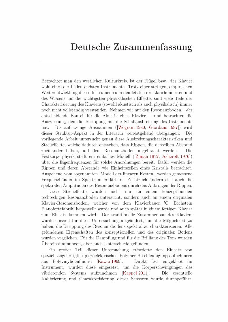
To generate a piano tone, a sequence of individual steps needs to be carriedout successively [Fletcher 1993, Conklin Jr. 1990] (schematic view of a pianois shown in Fig. 2.2): The initial step is pressing down one of the pianokeys. Since it is pressed, the string damper is raised and a hammer is directlyaccelerated to the string [Askenfelt 1993, Hall 1992a, Chaigne 1994b]. Whenit is thrown against the string [Suzuki 1987], a large amount of force in a shorttime is transferred to excite the string by that single pulse. That means, thedelivery of momentum from the hammer to the strings initializes the chain ofprocesses, which is needed for the generation of a piano tone. Not to interferewith the vibration, the hammer quickly departs from the string and if thepiano player wants to end the tone, he simply releases the key to drop thedamper against the string again, stopping the vibration and the respectiveradiation. Striking the key harder (i.e. increasing the force) over the sametime, the momentum and the vibration amplitude will increase. On the otherhand, a softer key excitation will result in a lower momentum and thereforea smaller amplitude of the string vibration. Because of that, the piano tone
2[Conklin Jr. 1996b] investigated tonal differences of historic and present soundboards.3With Helmholtz resonators one can investigate spectral fractions of a tone
[v. Helmholtz 1863].
8 Chapter 2. Background
Figure 2.2: Cross Section of a Piano with its most important parts for the sound
generation [Conklin Jr. 1990].
becomes minor and softer [Suzuki 2007]. The loudest acoustic output of apiano in units of power P is in the order of P = 0.1W, which seems to berelatively small, but is nevertheless the most of all compared to the majorityof all stringed instruments.
Depending on the frequency, a certain number of strings with (almost) thesame tuning contribute to one tone [Weinreich 1977, Fletcher 1993]. Thesestrings are hit by the same felt hammer. The higher the fundamentalfrequency of the piano tone, the higher the number of excited strings; rangingfrom one string for the low pitched sound, over two strings for the middlerange to three strings for the high pitch range. As indicated above, thestrings for the same tone are slightly detuned in order to extend the tonedecay [Weinreich 1977]. Once the momentum is transfered, the stringsbegin to couple their vibrations using the bridge for the connection. Thegentle tone generated by the string has to be magnified, because it is justuneffective concerning the sound radiation. When the string is actuallyexcited, the vibration is transfered from the string via the piano bridge tothe resonance board, which is a more efficient radiator of sound and actsas a loudspeaker for the string vibrations [Conklin Jr. 1996b, Giordano 1996,Giordano 1998b]. But during this process, another problem occurs: there isa significant difference in the mechanical impedance4 between the string andthe soundboard [Giordano 1998a]. From the perspective of the string, thesoundboard is just to heavy to be moved – the string vibrations are repeatedlyreflected at the bridge and they are slowly leaking into the soundboard. Butthis mismatch can be reduced by increasing the weight or the tension of thestrings [Conklin Jr. 1996d], which is practically being done by the commoncopper wrapping of the steel core strings (increasing the weight) and also bythe above mentioned ’multiple stringing’ per tone (increasing the tension).With these design modifications the transfer of the vibrations towards theresonance board becomes more efficient.
4The mechanical impedance describes the level of motional resistance of an object
exposed to an external force (see A.2.9.1).
2.1. The Piano 9
The sound radiation and the characteristics of a vibrating resonanceboard, which is one of the main parts of this investigation, is described in[Moore 2006, Conklin Jr. 1996b, Giordano 1998a, Suzuki 1986, Wogram 1980,Bork 1993, Giordano 2006] and will be he highlighted in the next section.
Another important aspect and a further longstanding goal in thepiano physics was the development of theoretical models, which areable to compute the sound characteristics or even mimicking theradiation. These models typically cover single individual steps in thetone generation sequence: the hammer motion [Hayashi 1999], thehammer-string interaction [Hall 1992b, Vyasarayani 2009, Komano 1994,Chaigne 1994a, Chaigne 1994c], the string vibration [Young 1952,Tufillaro 1995, Tufillaro 1989, Tanaka 1996, Ducasse 2005, Bensa 2003],and the soundboard vibration [Mamou-Mani 2008, Bensa 2005]. In the end,they help to provide important understanding of how the performance ofthe piano is changed by different modifications of individual instrumentparameters.
2.1.3 Soundboard and Ribs
The soundboard is typically a thin panel (thickness between 6 – 10mm) madeout of Norway spruce or Sitka spruce [Conklin Jr. 1996c, Yoshikawa 2007],underlying the piano strings and resting upon the wooden frame of thepiano. Dried to a very low moisture content [Fukada 1950], the wood is cuttype-dependently into strips with a width from 5cm to 15cm. Then the edgesof the stripes are glued together, preferring one direction for the wood grain.
The whole soundboard comprises not only the thin wooden panel, but alsothe supporting ribs mounted on its rear side and the two bridges (treble andbass) on the front side, which are the connections between the board and thestrings [Fletcher 1993, Conklin Jr. 1996b]. Acting as a natural resonator, thematerial and the design of the soundboard makes it very stiff concerning itsweight, and therefore it can be excited by the strings due to its lightness[Giordano 1998a]. Typically, the soundboard is curved with the highestpoint in the middle of the board; the form is then called ’the crown of thesoundboard’ [Mamou-Mani 2008]. Also made out of spruce and cut along thewood grain, the specially fitted ribs are the reason for this curvature. They aremounted perpendicular to the wood grain of the soundboard and glued to theboard with a rib press, which also accurately fixes their positions during thisprocedure. Finally mounted, they force the board into the above mentionedcrown form. Furthermore, the placed ribs will not only have the effect ofan increase of stiffness of the board [Giordano 1997]. They also pre-stressthe soundboard, which acts as an energy reservoir, releasing the vibrational

10 Chapter 2. Background
Figure 2.3: (Graph
taken from
[Conklin Jr. 1996c].)
Six different vibration
modes nicely presented
as Chladni figures on a
grand piano
soundboard. From top
left to bottom left:
first mode (49 Hz),
second mode (66.7 Hz)
and third mode (89.4
Hz). From top right to
bottom right: fourth
mode (112.8 Hz),
eighth mode (184 Hz)
and eleventh mode
(306 Hz).
energy in case. They additionally have the purpose to ’homogenize’ the boardin terms of stiffness parallel and perpendicular to the grain. The increasing ofthe stiffness will typically happen in two different ways: If the ribs’ Young’smodulus is larger than that of the soundboard, the overall modulus willenhance. Secondly, they increase the thickness of the soundboard h, whichyields a higher rigidity (see Eq. 2.1) and therefore the stiffness.
The treble and bass bridges transmit the string vibrations along theirwhole lengths to the soundboard. While the long treble bridge crossesthe high pitch strings, the bass bridge connects the bass strings withthe soundboard. The requirements for the bridges comprise a wide field:Going parallel to the grain of the soundboard, they also have to followthe crown form of the board. Moreover, the level of the upper end of thebridge is slightly higher than the string niveau, because the bridges haveto support the strings in the down-bearing process of the soundboard crown[Mamou-Mani 2008, Moore 2006]. Otherwise the tone produced by the stringswould drop. Therefore, to withstand the generated pressure between stringsand board, the bridge material is made of rigid solid blocks of wood, typicallymaple or beech.
The structure of the soundboard, considering the wood grain and itsdirections, is highly anisotropic and the equations of motion of a simple
2.1. The Piano 11
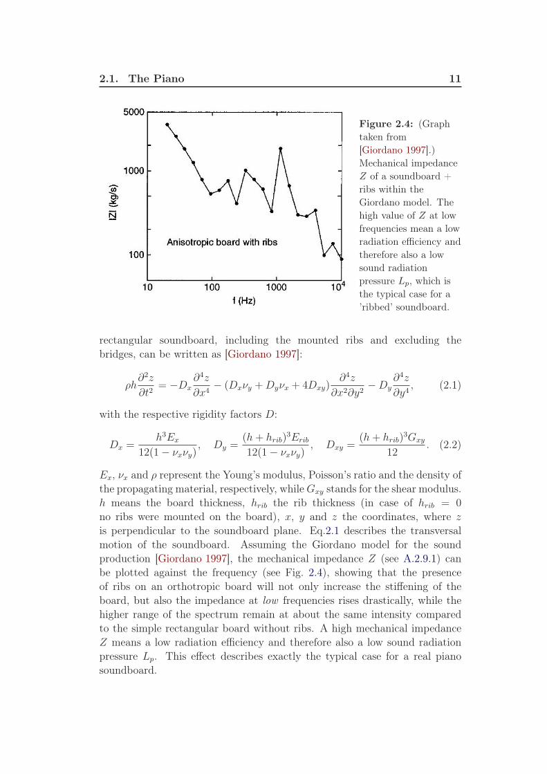
Figure 2.4: (Graph
taken from
[Giordano 1997].)
Mechanical impedance
Z of a soundboard +
ribs within the
Giordano model. The
high value of Z at low
frequencies mean a low
radiation efficiency and
therefore also a low
sound radiation
pressure Lp, which is
the typical case for a
’ribbed’ soundboard.
rectangular soundboard, including the mounted ribs and excluding thebridges, can be written as [Giordano 1997]:
ρh∂2z
∂t2= −Dx
∂4z
∂x4− (Dxνy +Dyνx + 4Dxy)
∂4z
∂x2∂y2−Dy
∂4z
∂y4, (2.1)
with the respective rigidity factors D:
Dx =h3Ex
12(1− νxνy), Dy =
(h+ hrib)3Erib
12(1− νxνy), Dxy =
(h+ hrib)3Gxy
12. (2.2)
Ex, νx and ρ represent the Young’s modulus, Poisson’s ratio and the density ofthe propagating material, respectively, whileGxy stands for the shear modulus.h means the board thickness, hrib the rib thickness (in case of hrib = 0
no ribs were mounted on the board), x, y and z the coordinates, where zis perpendicular to the soundboard plane. Eq.2.1 describes the transversalmotion of the soundboard. Assuming the Giordano model for the soundproduction [Giordano 1997], the mechanical impedance Z (see A.2.9.1) canbe plotted against the frequency (see Fig. 2.4), showing that the presenceof ribs on an orthotropic board will not only increase the stiffening of theboard, but also the impedance at low frequencies rises drastically, while thehigher range of the spectrum remain at about the same intensity comparedto the simple rectangular board without ribs. A high mechanical impedanceZ means a low radiation efficiency and therefore also a low sound radiationpressure Lp. This effect describes exactly the typical case for a real pianosoundboard.

12 Chapter 2. Background
But how does the small radiation efficiency for the low spectral range comefrom, when it was already mentioned in the last section that a soundboard canbe a significantly efficient radiator of airborne sound waves? The reason canbe found indeed by the frequency dependence of the efficiency. Typically, lowfrequencies (see Fig 2.4) are less efficiently radiated, because the wavelengthis just long enough to be acoustically ’short-circuited’ around the board[Bork 1993, Fletcher 1999, Wogram 1980], i.e. the compressed air on one sideof the soundboard has enough time to be moved to the other side of theboard with the reduced pressure. By neutralizing this difference through theexchange of air, the radiation efficiency drops drastically5. But even at higherfrequencies a similar effect can occur when certain vibrational modes (SeeFig. 2.3 for exemplary modes) cancel out each other [Wogram 1980]. Theseeigenmodes vibrate in an opposite phase, i.e. one area of the soundboardis moving upwards, while a neighbour region is moving downwards. Hence,the radiation efficiency at these specific modes, which are the ’valleys’ in thespectrum, are significantly reduced by the air exchange of the neighbouringregions. However, if the vibrational transfer is too efficient, the piano tonewill decay too early. That would mean the tone is too loud and too short. Toachieve a compromise, a relatively large part of the vibrational energy needsto be reflected back into the strings.
There are certain rib parameters concerning the spectral radiation, whichcan be varied. [Wogram 1980] performed investigations on the influence ofthe rib height and their numbers on the soundboard. When the rib heightwas reduced gradually, he found at the upper end of the treble bridge nosignificant change in the input impedance. However, the central region of thesoundboard revealed the evolution of pronounced resonances of the impedancebelow 200 Hz. Also the resonant frequencies are shifted downwards when therib height was decreased, while their extrema become more sharply defined.Nevertheless, no uniform correlation relating the rib height and the impedancevariation was found. He finally concluded, that the bending stiffness exertsa greater influence on the sound radiation than the mass of the ribs andtherefore it is more fortunate for the radiation characteristic of a soundboardto use narrow, high ribs than low and broad ones (i.e. increasing the stiffnesswithout increasing the mass in the same magnitude). He also investigatedthe occuring differences if the rib number on the rear side of the soundboardvaries and concluded that a change in the number of ribs has less influence onthe input impedance and the sound radiation than a change in rib height.
[Chaigne 2011] presented results at the ’Acoustical Society of America’
5This specific effect can be reduced by a closed sound box, which is realized for the
guitar and the violine [Fletcher 1999, Elejabarrieta 2002]

2.1. The Piano 13
(ASA) meeting 2011 about the ribbing influence of the soundboard radiation.He found that an aperiodicity of the ribs would result in a reduction of thespectral peak sharpness. The presence of the ribs would also result in adirectivity of the sound radiation, but the main findings are again that theribs will enhance the stiffening of the soundboard.
2.1.4 Scattering generated by the Ribs
In the course of this investigation ribs will be placed onto a radiatingsoundboard, i.e. a regular assembly is added to the radiator. Consideringthese specific add-ons, a model about the sound radiation and the frequencyselection by scattering will be necessary. The solid-state physics canhold for such a model – the so-called linear chain model (LCM). Sinceit is very important for the explanation of the later occuring scatteringeffects, the LCM model will be presented in this section. It highlightsthe evolving dispersion relation and distinguishes between ’allowed’ and’forbidden’ frequencies (In this case ’allowed’ means the frequencies arepart of the solution of the LCM model; ’forbidden’ refers to no solution),if a given setup is excited. The propagating ’pass band’ frequencies,allowed by the external scattering circumstances, are travelling waves.
(a)
(b)
Figure 2.5: (a): 1-dim infinitely extended linear
chain of masses with the respective dispersion
relation in (b). This represents the basis for the
LCM model, where only the nearest-neighbor
forces are considered.
One of the pivotaladvantages to referringto this model is thatin constrast to surfacevibrations, which followa fourth order waveequation (see Eq. 2.1),body vibrations along acertain direction can bedescribed by a secondorder wave equation,reducing the complexityof the problem significantly.A description of thatscattering model, whichsets each individualrib as a scattereris described in thissection. A more profunddescription is provided in[Ashcroft 1976, Morse 1987, Ziman 1972, Kittel 1953].
14 Chapter 2. Background
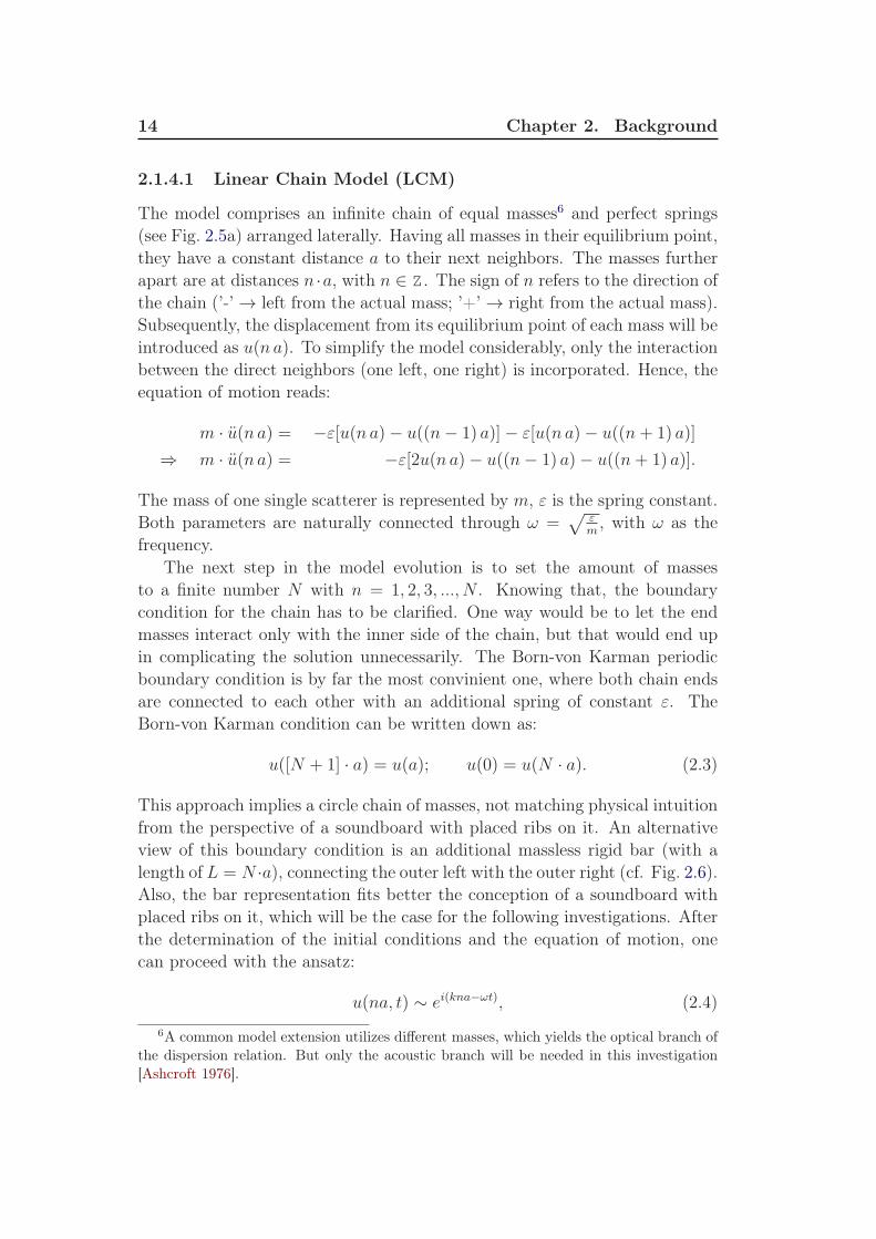
2.1.4.1 Linear Chain Model (LCM)
The model comprises an infinite chain of equal masses6 and perfect springs(see Fig. 2.5a) arranged laterally. Having all masses in their equilibrium point,they have a constant distance a to their next neighbors. The masses furtherapart are at distances n ·a, with n ∈ Z. The sign of n refers to the direction ofthe chain (’-’ → left from the actual mass; ’+’ → right from the actual mass).Subsequently, the displacement from its equilibrium point of each mass will beintroduced as u(n a). To simplify the model considerably, only the interactionbetween the direct neighbors (one left, one right) is incorporated. Hence, theequation of motion reads:
m · u(n a) = −ε[u(n a)− u((n− 1) a)]− ε[u(n a)− u((n+ 1) a)]
⇒ m · u(n a) = −ε[2u(n a)− u((n− 1) a)− u((n+ 1) a)].
The mass of one single scatterer is represented by m, ε is the spring constant.Both parameters are naturally connected through ω =
√
εm
, with ω as thefrequency.
The next step in the model evolution is to set the amount of massesto a finite number N with n = 1, 2, 3, ..., N . Knowing that, the boundarycondition for the chain has to be clarified. One way would be to let the endmasses interact only with the inner side of the chain, but that would end upin complicating the solution unnecessarily. The Born-von Karman periodicboundary condition is by far the most convinient one, where both chain endsare connected to each other with an additional spring of constant ε. TheBorn-von Karman condition can be written down as:
u([N + 1] · a) = u(a); u(0) = u(N · a). (2.3)
This approach implies a circle chain of masses, not matching physical intuitionfrom the perspective of a soundboard with placed ribs on it. An alternativeview of this boundary condition is an additional massless rigid bar (with alength of L = N ·a), connecting the outer left with the outer right (cf. Fig. 2.6).Also, the bar representation fits better the conception of a soundboard withplaced ribs on it, which will be the case for the following investigations. Afterthe determination of the initial conditions and the equation of motion, onecan proceed with the ansatz:
u(na, t) ∼ ei(kna−ωt), (2.4)
6A common model extension utilizes different masses, which yields the optical branch of
the dispersion relation. But only the acoustic branch will be needed in this investigation
[Ashcroft 1976].

2.1. The Piano 15
Figure 2.6: Born-von Karman boundary condition: A rigid massless bar connects
both ends of the mass chain, which fits the conception of a soundboard with
mounted ribs in a better way.
having in mind that the periodic7 boundary condition needs to fulfill:
eikNa = 1. (2.5)
That, on the other hand, restricts k to
k =2π
a· nN, (2.6)
where n has to be an integer. The range of −π/a < k < π/a fully comprisesthe first Brillouin zone. Any change by 2π/a has no effect on the displacementu(na). Therefore, only N distinguishable solutions exist for this equation ofmotion.
The following step is to insert the ansatz into the equation of motion.Hence,
−mω2ei(kna−ωt) =− ε[2− e−ika − eika] · ei(kna−ωt)
⇒ ω2 =ε
m· [2− 2 cos(ka)]
⇒ ω(k) =2 ·√
ε
m· | sin(ka/2)|.
The ’acoustic branch’ solution for the eigenmodes will emerge (see[Ziman 1972, Ashcroft 1976]), if k (Eq. 2.6) is considered:
ω(n) = 2 ·√
ε
m· | sin(π · n/N)|. (2.7)
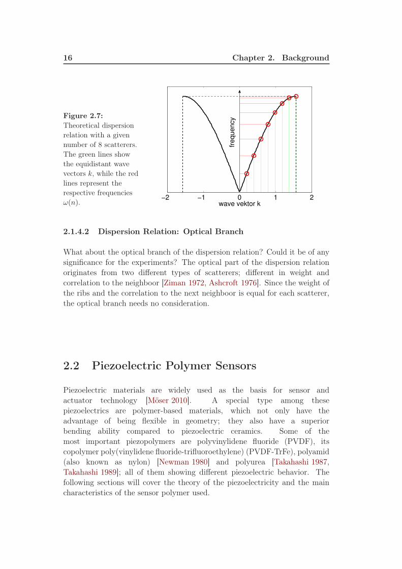
The frequency ω vs. wave vektor k is plotted in the range of the first Brillouinzone (cf. Fig. 2.7), showing the frequency distribution of the allowed ’passbands’.
7Despite the bar repesentation of the chain, there is of course a periodic boundary
condition.
16 Chapter 2. Background
Figure 2.7:
Theoretical dispersion
relation with a given
number of 8 scatterers.
The green lines show
the equidistant wave
vectors k, while the red
lines represent the
respective frequencies
ω(n).−2 −1 0 1 2
wave vektor k
fre
qu
en
cy
2.1.4.2 Dispersion Relation: Optical Branch
What about the optical branch of the dispersion relation? Could it be of anysignificance for the experiments? The optical part of the dispersion relationoriginates from two different types of scatterers; different in weight andcorrelation to the neighboor [Ziman 1972, Ashcroft 1976]. Since the weight ofthe ribs and the correlation to the next neighboor is equal for each scatterer,the optical branch needs no consideration.
2.2 Piezoelectric Polymer Sensors
Piezoelectric materials are widely used as the basis for sensor andactuator technology [Möser 2010]. A special type among thesepiezoelectrics are polymer-based materials, which not only have theadvantage of being flexible in geometry; they also have a superiorbending ability compared to piezoelectric ceramics. Some of themost important piezopolymers are polyvinylidene fluoride (PVDF), itscopolymer poly(vinylidene fluoride-trifluoroethylene) (PVDF-TrFe), polyamid(also known as nylon) [Newman 1980] and polyurea [Takahashi 1987,Takahashi 1989]; all of them showing different piezoelectric behavior. Thefollowing sections will cover the theory of the piezoelectricity and the maincharacteristics of the sensor polymer used.
2.2. Piezoelectric Polymer Sensors 17
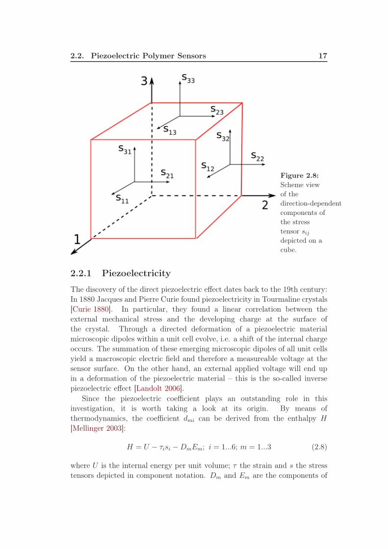
Figure 2.8:
Scheme view
of the
direction-dependent
components of
the stress
tensor sijdepicted on a
cube.
2.2.1 Piezoelectricity
The discovery of the direct piezoelectric effect dates back to the 19th century:In 1880 Jacques and Pierre Curie found piezoelectricity in Tourmaline crystals[Curie 1880]. In particular, they found a linear correlation between theexternal mechanical stress and the developing charge at the surface ofthe crystal. Through a directed deformation of a piezoelectric materialmicroscopic dipoles within a unit cell evolve, i.e. a shift of the internal chargeoccurs. The summation of these emerging microscopic dipoles of all unit cellsyield a macroscopic electric field and therefore a measureable voltage at thesensor surface. On the other hand, an external applied voltage will end upin a deformation of the piezoelectric material – this is the so-called inversepiezoelectric effect [Landolt 2006].
Since the piezoelectric coefficient plays an outstanding role in thisinvestigation, it is worth taking a look at its origin. By means ofthermodynamics, the coefficient dmi can be derived from the enthalpy H
[Mellinger 2003]:
H = U − τisi −DmEm; i = 1...6; m = 1...3 (2.8)
where U is the internal energy per unit volume; τ the strain and s the stresstensors depicted in component notation. Dm and Em are the components of

18 Chapter 2. Background
the electric displacement D and the electric field E. The full representationfor τ and s are 3 x 3 matrices τkl and skl with all components of the stresstensor depicted on a cube in Fig. 2.8. Both tensors are symmetric with only6 independent components: s = (s11, s22, s33, s23, s12, s12). The notation canbe simplifyed by the so-called 1-dimensional Voigt notation: si with i = 1...6.Thus, the adiabatic piezoelectric strain coefficient dmi reads:
dmi = −(
∂2H
∂Em∂si
)
S
(2.9)
The index S denotes that the entropy remains constant. The derivation ofthe enthalpy is complete and can be written as:
dH = −τidsi −DmdEm + TdS (2.10)
Since this differential can be taken in arbitrary order, the adiabaticpiezoelectric strain coefficient dmi is represented by:
dmi =
(
∂Dm
∂si
)
E,S
=
(
∂τi∂Em
)
s,S
(2.11)
The left-hand side of Eq. 2.11 describes the direct piezoelectric effect, i.e. anelectric displacement caused by mechanical stress. The ( ∂τi
∂Em)s,S term shows
the inverse piezoelectric effect, where a dimensional change is caused by anelectric field.
2.2.2 Material: Why Polyvinylidene Fluoride?
Polyvinylidene fluoride (PVDF) (see Fig. 2.9) has a wide range of applicationsdue to its specific mechanical and electrical properties ([Sessler 1999b,Bauer 2004, Zhang 2002, Vinogradov 2002, Tasaka 1981, Nix 1986]). Itconsists of a repeat unit with the molecular formula (CH2 − CF2)n and exibits,after external poling (see Fig. 2.11c.), one of the strongest piezoelectricbehavior within all known polymers (Tab. 2.1 shows several characteristicscompared with other materials) [Sessler 1981]. Since the discovery ofits piezoelectricity [Kawai 1969], PVDF has become one of the workinghorses in sensor applications as acoustic transducer and electromechanicalactuator. Other crucial advantages for using PVDF are based on itsbending ability, ultra-thin dimensions (few micrometers; typical thicknessof 30µm) and the high geometric flexibility to fit in every desired form.

2.2. Piezoelectric Polymer Sensors 19
Sensor material [g/cm3] v [m/s] d [pC/N] Z [103 · Ns/m3]PVDF (β-phase) 1.78 2300 d33 = 20− 30 ∼ 4PVDF (δ-phase) 1.78 2300 d33 = 10− 15 ∼ 4
PZT 7.5 2700 d31 = 100− 300 ∼ 20barium titanate 6.0 3200 d31 = 80 ∼ 19
quartz 2.7 3750 d31 = 2 ∼ 10
Table 2.1: Typical characteristics (physical and piezoelectric) for common sensor
materials [MSI 2006]. Density , longitudinal velocity vc, piezoelectric coefficient d
and the acoustic impedance Z (see Sec. A.2.9.1, enlisted respectively. PZT refers
to lead zirconate titanate, a commonly used piezoelectric ceramic.
Figure 2.9: Chemical
formula of
polyvinylidene fluoride
as a repeat unit
[Kawai 1969].
In addition, PVDF is predestined to be used formeasuring solid-state sound vibrations in wood andsynthetics due to the specific acoustic impedanceZ (see Sec. A.2.9.1 and Tab. 2.1 for the specificvalues) because Zwood is just a half magnitude belowZPVDF [Bucur 2006, MSI 2006]. ZPVDF is closer toZwood compared to the acoustic impedance of othertypical piezoelectric materials (see again Tab. 2.1).Therefore, internal sound wave reflections at thematerial interfaces are reduced to a minimum andthese effects can be safely neglected for the smallobstacles used in this investigation. It should benoted here, that PVDF has a negative piezoelectriceffect, meaning that it will compress instead ofexpand when exposed to the same electric field[Pu 2010]. This behavior is different in contrast to other piezoelectricmaterials like PZT, which have a positive piezoelectric effect.
2.2.3 PVDF Morphology & Piezoelectricity
PVDF is one of the most important fluoropolymers, having four differentcrystallite modifications, know as the α, β, γ and δ phase, which areadditionally referred as form I (β phase), form II (α phase), form IIp (δ phase,which is actually the polar form II) and form III (γ phase) (see Fig. 2.10a& b). Since it is the thermodynamically most stable form of PVDF, thenon-polar α phase makes up the biggest share in melt-processed films. Thephases α and δ actually have the same molecular configuration, but theycrystallize in a different manner. While the α phase is arranged such thatthe dipole moment of the different molecular chains is zero (cf. Fig. 2.10b
20 Chapter 2. Background
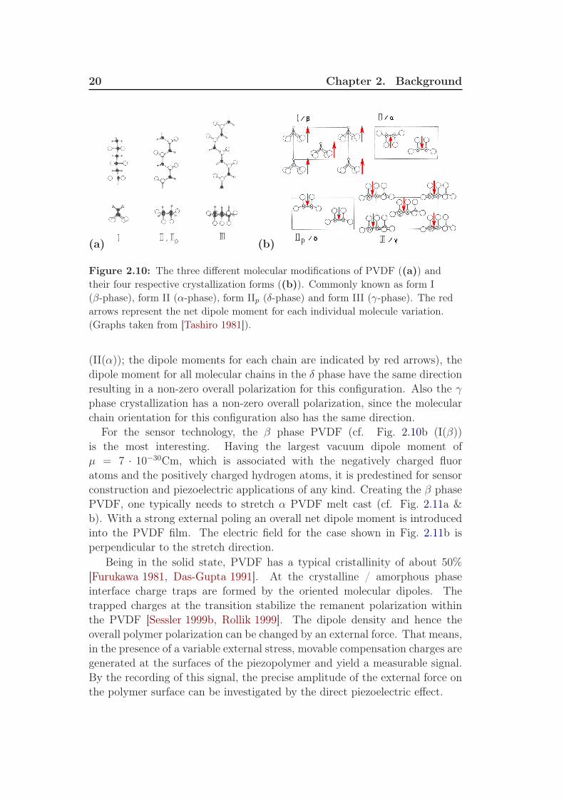
(a) (b)
Figure 2.10: The three different molecular modifications of PVDF ((a)) and
their four respective crystallization forms ((b)). Commonly known as form I
(β-phase), form II (α-phase), form IIp (δ-phase) and form III (γ-phase). The red
arrows represent the net dipole moment for each individual molecule variation.
(Graphs taken from [Tashiro 1981]).
(II(α)); the dipole moments for each chain are indicated by red arrows), thedipole moment for all molecular chains in the δ phase have the same directionresulting in a non-zero overall polarization for this configuration. Also the γphase crystallization has a non-zero overall polarization, since the molecularchain orientation for this configuration also has the same direction.
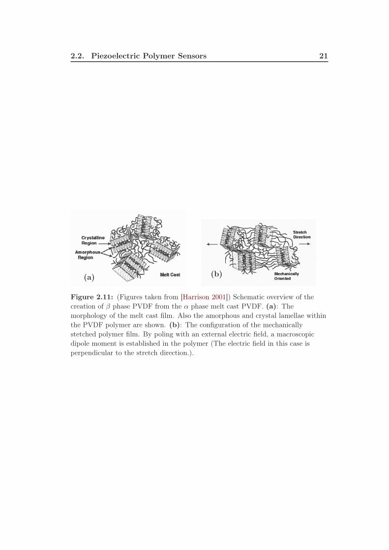
For the sensor technology, the β phase PVDF (cf. Fig. 2.10b (I(β))is the most interesting. Having the largest vacuum dipole moment ofµ = 7 · 10−30Cm, which is associated with the negatively charged fluoratoms and the positively charged hydrogen atoms, it is predestined for sensorconstruction and piezoelectric applications of any kind. Creating the β phasePVDF, one typically needs to stretch α PVDF melt cast (cf. Fig. 2.11a &b). With a strong external poling an overall net dipole moment is introducedinto the PVDF film. The electric field for the case shown in Fig. 2.11b isperpendicular to the stretch direction.
Being in the solid state, PVDF has a typical cristallinity of about 50%[Furukawa 1981, Das-Gupta 1991]. At the crystalline / amorphous phaseinterface charge traps are formed by the oriented molecular dipoles. Thetrapped charges at the transition stabilize the remanent polarization withinthe PVDF [Sessler 1999b, Rollik 1999]. The dipole density and hence theoverall polymer polarization can be changed by an external force. That means,in the presence of a variable external stress, movable compensation charges aregenerated at the surfaces of the piezopolymer and yield a measurable signal.By the recording of this signal, the precise amplitude of the external force onthe polymer surface can be investigated by the direct piezoelectric effect.
2.2. Piezoelectric Polymer Sensors 21
(a) (b)
Figure 2.11: (Figures taken from [Harrison 2001]) Schematic overview of the
creation of β phase PVDF from the α phase melt cast PVDF. (a): The
morphology of the melt cast film. Also the amorphous and crystal lamellae within
the PVDF polymer are shown. (b): The configuration of the mechanically
stetched polymer film. By poling with an external electric field, a macroscopic
dipole moment is established in the polymer (The electric field in this case is
perpendicular to the stretch direction.).


Chapter 3
Measurement Techniques
The present chapter consists of two sections. The conceptional soundboardmeasurements (described in chapter 4) were carried out inside an anechoicchamber. Therefore, the characterization and classification of the recordingroom will be discussed in the first part of this chapter. The second partis about specially prepared piezoelectric polymer sensors, which are able torecord solid-state vibrations. This section comprises the full description andthe pivotal calibration and characterization. Finally, there is a brief sectionat the end of this chapter about condenser microphones, which were used forthe airborne sound measurements throughout this investigation.
3.1 Characterization of the Measurement
Room
Within a measurement room an acoustic wave can be perturbated by twoeffects [Möser 2007]: Interferences with ambient noise from outside the roomand reflected sound waves within the room are possible. Both effects shouldbe minimized, because they can have a huge impact on the time signal and thespectrum. Naturally, it is impossible to eliminate these perturbation effectscompletely, but they should be limited to a certain niveau within the spectraldata acquisition range. Only in this case one can obtain scientific statementsabout the investigated signal with some certainty.
For the reduction of the reflected sound waves [Möser 2007] we need anattenuation material on the inner surface of the measurement chamber, whichwas done by a layer of mineral wool and additional specially manufacturedpyramid foam, which is described below. Special material at the outer wall ofthe room reduces the influence of the external ambient noise by soundproofing.Both mechanisms rely on different physical principles: While by soundproofingthe external perturbation sound waves are reflected more efficiently from themeasurement chamber, the absorption layer depletes the amplitude of thesignal via friction within the material. All characterization measurements ofthe recording chamber will be given in the following. With these investigatedparameters the room is fully acoustically classified according to the DIN e.V.norm ([DIN e.V. 2005a, DIN e.V. 2005b]).

24 Chapter 3. Measurement Techniques
3.1.1 Geometry & Material
The acoustic laboratory consists of a normal room (without soundproofingand absorption layer) in which most of the recording devices are located andinstalled. Within this room another room is built (see Fig. 3.1a), whichis the actual acoustic measurement chamber. It stands 0.57m away fromthe surrounding walls of the outer room. Because these two chambers arenot interconnected – except for the floor naturally – possible influences frombuilding vibrations, which certainly exist and are measureable (e.g. closingdoors, ventilation or even a person passing by), are reduced to a minimum.
The outer wall of the recording room is 23cm in thickness (without innerabsorption layer) and consists of two individual gypsum plaster boards 2.65cmin thickness. They are 17.5cm in distance from each other. The gap betweenthose boards is completely filled with mineral wool. Gypsum plaster boardsare easy to handle for constructions, but unfortunately their density is prettylow (gypsum = 2.3g/cm3) compared to other material, which is used for roomconstruction. Typically, the higher the density, the higher the ability toreflect airborne sound waves, due to the larger acoustic impedance mismatch(see A.2.9.1). Nevertheless one can assume, due to the big mineral-wool-filledcavity between the two plates, a certainly good damping factor for the outerambient noise. The inner surface of the recording room is permanently coveredwith a combination of two different damping materials: the basis is formed bya 8cm thick mineral wool layer (see Fig. 3.1b), whereas the top layer is madeof special acoustic pyramid foam (see Fig. 3.1c). The floor is also covered witha mineral wool layer and to be able to enter the room a metal grid is installed.
The dimension of the recording room (without the absorption layers) is3.075m x 3.13m x 3.23m in width, length, and height respectively. Thereforeone has a volume of V ≃ 31m3 and a surface area of S ≃ 60m2. If asound source is placed in the middle of the room, the distance between thesource and the wall is 1.46m (subtracting the absorber layer). The literature[DIN e.V. 2005a, DIN e.V. 2005b] defines the lower frequency confidence levelof a measurement room as the minimum distance of one wavelength (fromsound source to the inner wall). For the air temperature of 20C that can becalculated by:
fconf ≈ cairλ
=343m
s
1, 46m≈ 230Hz (3.1)
fconf represents the lower limit for trustworthy results obtained in thismeasurement room. On a later point this will be verified by the roomcharacterization measurement (see 3.1.2.2).

3.1. Characterization of the Measurement Room 25
a) b)
c)
Figure 3.1: a): Overview of the acoustic measurement room seen through the
door. The metal grid used for the entering of the room is seen beside some
equipment. b): Side view of the 8cm thick absorption material made out of
mineral wool.
c): Showing the finally attached pyramid aborption layer of the anechoic chamber
(See Sec. 3.1.1 for description.).
3.1.2 Sound Wave Absorption
3.1.2.1 Specification
The pivotal aim of sound wave absorption is to reduce the field of soundwaves on a wide frequency range within the recording room. Due to innerfriction within the absorption foam the amplitude of the reflected sound waveis reduced. In Eq. 3.1 the lower confidence level of the measurement chamberwas found at about 230Hz. For higher frequencies, the absorption of the innerlayers is very good.
For the special pyramid foam on top of the mineral wool layer, thefrequency-dependent sound wave absorption coefficient α was provided fromthe manufacturer ’Pinta Acoustics GmbH’. Regarding the overall absorptionlayer (including the underlying 8cm mineral wool), this setup is very close tothe ’pinta pyramid 100/50’ configuration in terms of thickness and material,having absoption coefficient values given in Tab. 3.1.
26 Chapter 3. Measurement Techniques
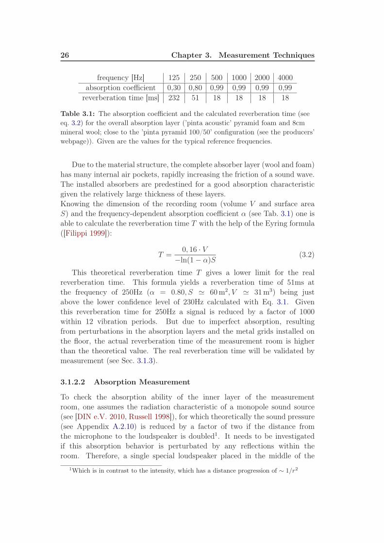
frequency [Hz] 125 250 500 1000 2000 4000absorption coefficient 0,30 0,80 0,99 0,99 0,99 0,99
reverberation time [ms] 232 51 18 18 18 18
Table 3.1: The absorption coefficient and the calculated reverberation time (see
eq. 3.2) for the overall absorption layer (’pinta acoustic’ pyramid foam and 8cm
mineral wool; close to the ’pinta pyramid 100/50’ configuration (see the producers’
webpage)). Given are the values for the typical reference frequencies.
Due to the material structure, the complete absorber layer (wool and foam)has many internal air pockets, rapidly increasing the friction of a sound wave.The installed absorbers are predestined for a good absorption characteristicgiven the relatively large thickness of these layers.Knowing the dimension of the recording room (volume V and surface areaS) and the frequency-dependent absorption coefficient α (see Tab. 3.1) one isable to calculate the reverberation time T with the help of the Eyring formula([Filippi 1999]):
T =0, 16 · V
−ln(1− α)S(3.2)
This theoretical reverberation time T gives a lower limit for the realreverberation time. This formula yields a reverberation time of 51ms atthe frequency of 250Hz (α = 0.80, S ≃ 60m2, V ≃ 31m3) being justabove the lower confidence level of 230Hz calculated with Eq. 3.1. Giventhis reverberation time for 250Hz a signal is reduced by a factor of 1000within 12 vibration periods. But due to imperfect absorption, resultingfrom perturbations in the absorption layers and the metal grids installed onthe floor, the actual reverberation time of the measurement room is higherthan the theoretical value. The real reverberation time will be validated bymeasurement (see Sec. 3.1.3).
3.1.2.2 Absorption Measurement
To check the absorption ability of the inner layer of the measurementroom, one assumes the radiation characteristic of a monopole sound source(see [DIN e.V. 2010, Russell 1998]), for which theoretically the sound pressure(see Appendix A.2.10) is reduced by a factor of two if the distance fromthe microphone to the loudspeaker is doubled1. It needs to be investigatedif this absorption behavior is perturbated by any reflections within theroom. Therefore, a single special loudspeaker placed in the middle of the
1Which is in contrast to the intensity, which has a distance progression of ∼ 1/r2
3.1. Characterization of the Measurement Room 27
0 5 10 15
10−6
10−5
10−4
10−3
frequency [kHz]
inte
nsity [a.u
.]
20cm
40cm
80cm
0 5 10 15
10−6
10−5
10−4
10−3
frequency [kHz]
inte
nsity [a.u
.]
30cm
60cm
120cm
(a) (b)
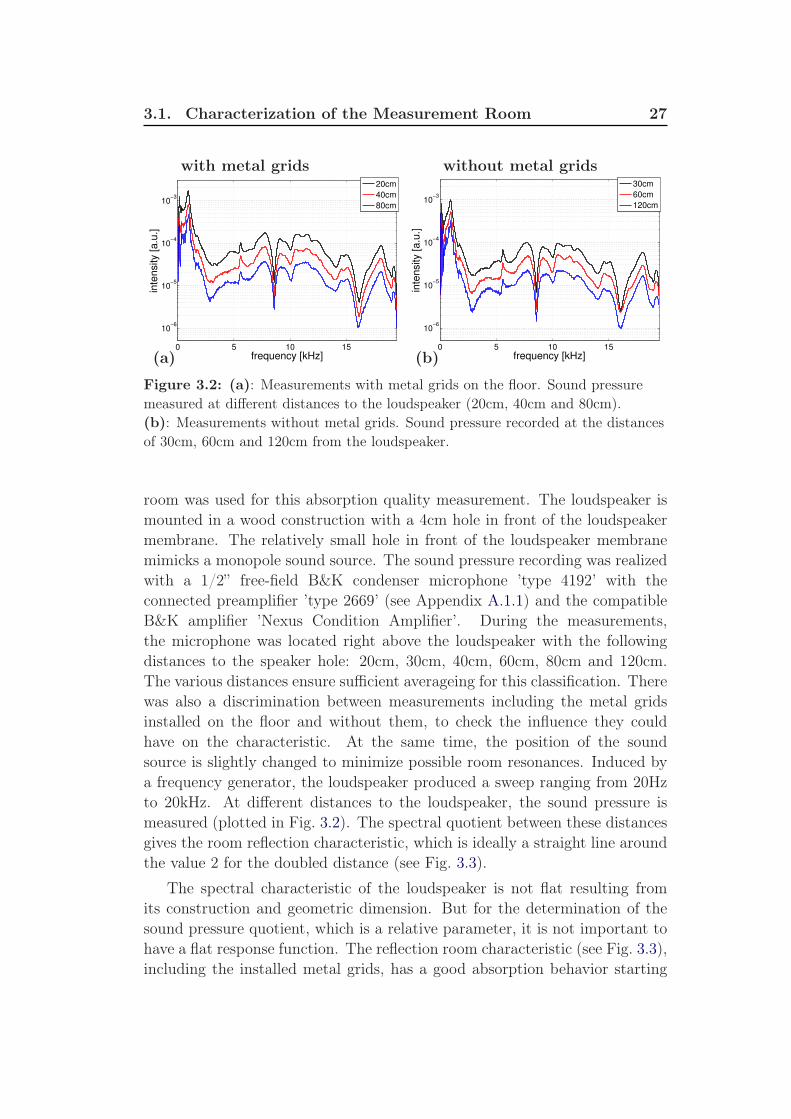
with metal grids without metal grids
Figure 3.2: (a): Measurements with metal grids on the floor. Sound pressure
measured at different distances to the loudspeaker (20cm, 40cm and 80cm).
(b): Measurements without metal grids. Sound pressure recorded at the distances
of 30cm, 60cm and 120cm from the loudspeaker.
room was used for this absorption quality measurement. The loudspeaker ismounted in a wood construction with a 4cm hole in front of the loudspeakermembrane. The relatively small hole in front of the loudspeaker membranemimicks a monopole sound source. The sound pressure recording was realizedwith a 1/2” free-field B&K condenser microphone ’type 4192’ with theconnected preamplifier ’type 2669’ (see Appendix A.1.1) and the compatibleB&K amplifier ’Nexus Condition Amplifier’. During the measurements,the microphone was located right above the loudspeaker with the followingdistances to the speaker hole: 20cm, 30cm, 40cm, 60cm, 80cm and 120cm.The various distances ensure sufficient averageing for this classification. Therewas also a discrimination between measurements including the metal gridsinstalled on the floor and without them, to check the influence they couldhave on the characteristic. At the same time, the position of the soundsource is slightly changed to minimize possible room resonances. Induced bya frequency generator, the loudspeaker produced a sweep ranging from 20Hzto 20kHz. At different distances to the loudspeaker, the sound pressure ismeasured (plotted in Fig. 3.2). The spectral quotient between these distancesgives the room reflection characteristic, which is ideally a straight line aroundthe value 2 for the doubled distance (see Fig. 3.3).
The spectral characteristic of the loudspeaker is not flat resulting fromits construction and geometric dimension. But for the determination of thesound pressure quotient, which is a relative parameter, it is not important tohave a flat response function. The reflection room characteristic (see Fig. 3.3),including the installed metal grids, has a good absorption behavior starting
28 Chapter 3. Measurement Techniques
0 5 10 150
1
2
3
4
5
6
frequency [kHz]
sp
ectr
al d
iffe
ren
ce
with metal grid
without metal grid
0 0.2 0.4 0.6 0.8 10
1
2
3
4
5
6
frequency [kHz]
sp
ectr
al d
iffe
ren
ce
with metal grid
without metal grid
(a) (b)
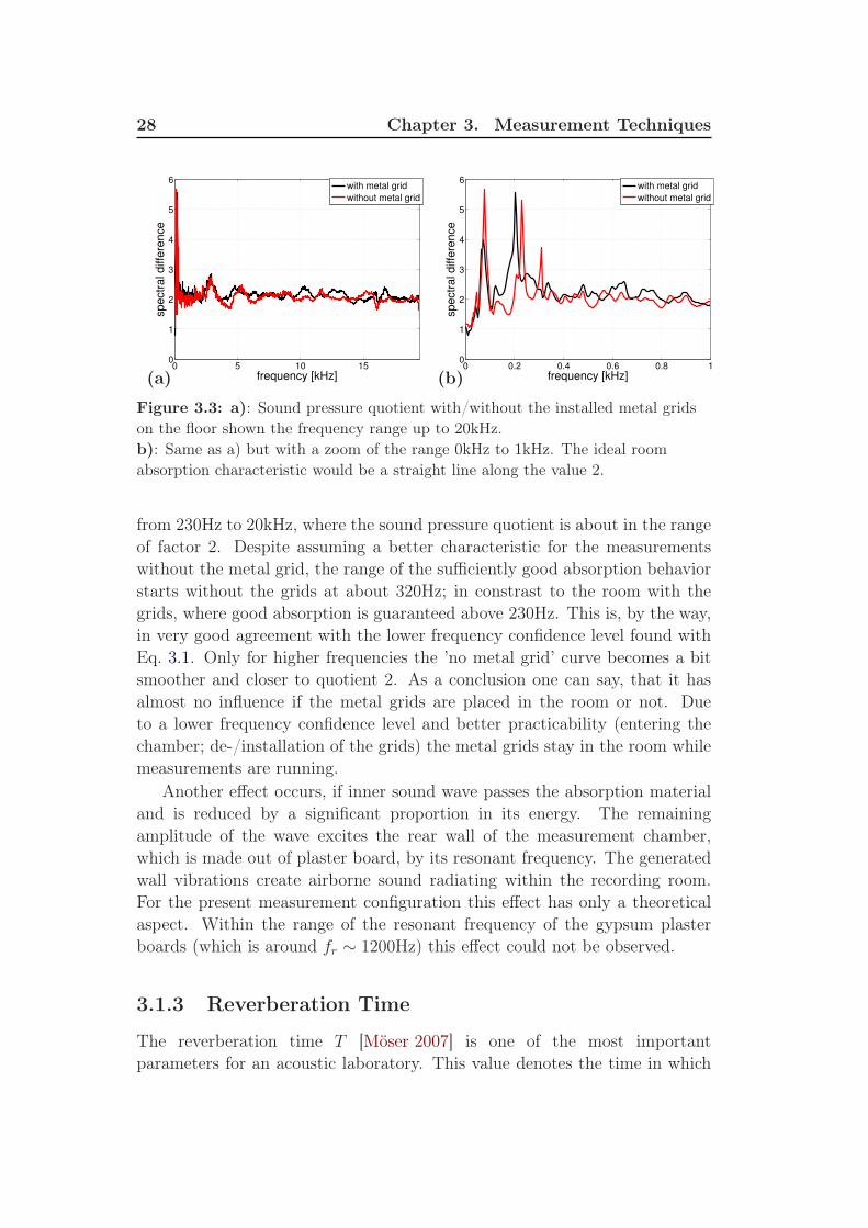
Figure 3.3: a): Sound pressure quotient with/without the installed metal grids
on the floor shown the frequency range up to 20kHz.
b): Same as a) but with a zoom of the range 0kHz to 1kHz. The ideal room
absorption characteristic would be a straight line along the value 2.
from 230Hz to 20kHz, where the sound pressure quotient is about in the rangeof factor 2. Despite assuming a better characteristic for the measurementswithout the metal grid, the range of the sufficiently good absorption behaviorstarts without the grids at about 320Hz; in constrast to the room with thegrids, where good absorption is guaranteed above 230Hz. This is, by the way,in very good agreement with the lower frequency confidence level found withEq. 3.1. Only for higher frequencies the ’no metal grid’ curve becomes a bitsmoother and closer to quotient 2. As a conclusion one can say, that it hasalmost no influence if the metal grids are placed in the room or not. Dueto a lower frequency confidence level and better practicability (entering thechamber; de-/installation of the grids) the metal grids stay in the room whilemeasurements are running.
Another effect occurs, if inner sound wave passes the absorption materialand is reduced by a significant proportion in its energy. The remainingamplitude of the wave excites the rear wall of the measurement chamber,which is made out of plaster board, by its resonant frequency. The generatedwall vibrations create airborne sound radiating within the recording room.For the present measurement configuration this effect has only a theoreticalaspect. Within the range of the resonant frequency of the gypsum plasterboards (which is around fr ∼ 1200Hz) this effect could not be observed.
3.1.3 Reverberation Time
The reverberation time T [Möser 2007] is one of the most importantparameters for an acoustic laboratory. This value denotes the time in which
3.1. Characterization of the Measurement Room 29
0.01 0.02 0.03 0.04 0.05 0.06−0.1
0
0.1
time [s]
am
plit
ude [a.u
.]
0.01 0.02 0.03 0.04 0.05 0.06
−40
−20
0
time [s]
sound p
ressure
[dB
]
0.01 0.015 0.02 0.025 0.03 0.035 0.04 0.045−0.2
0
0.2
time [s]
am
plit
ude [a.u
.]
0.01 0.015 0.02 0.025 0.03 0.035 0.04 0.045
−40
−20
0
time [s]
sound p
ressure
[dB
]
(a) (b)
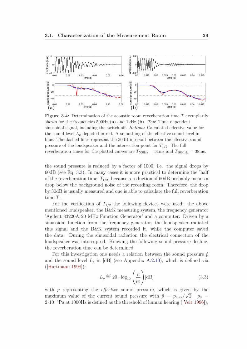
Figure 3.4: Determination of the acoustic room reverberation time T exemplarily
shown for the frequencies 500Hz (a) and 1kHz (b). Top: Time dependent
sinusoidal signal, including the switch-off. Bottom: Calculated effective value for
the sound level Lp depicted in red. A smoothing of the effective sound level in
blue. The dashed lines represent the 30dB intervall between the effective sound
pressure of the loudspeaker and the intersection point for T1/2. The full
reverberation times for the plotted curves are T500Hz = 51ms and T1000Hz = 38ms.
the sound pressure is reduced by a factor of 1000, i.e. the signal drops by60dB (see Eq. 3.3). In many cases it is more practical to determine the ’halfof the reverberation time’ T1/2, because a reduction of 60dB probably means adrop below the background noise of the recording room. Therefore, the dropby 30dB is usually measured and one is able to calculate the full reverberationtime T .
For the verification of T1/2 the following devices were used: the abovementioned loudspeaker, the B&K measuring system, the frequency generator’Agilent 33220A 20 MHz Function Generator’ and a computer. Driven by asinusoidal function from the frequency generator, the loudspeaker radiatedthis signal and the B&K system recorded it, while the computer savedthe data. During the sinusoidal radiation the electrical connection of theloudspeaker was interrupted. Knowing the following sound pressure decline,the reverberation time can be determined.
For this investigation one needs a relation between the sound pressure pand the sound level Lp in [dB] (see Appendix A.2.10), which is defined via([Hartmann 1998]):
Lp =def 20 · log10
(
p
p0
)
[dB] (3.3)
with p representing the effective sound pressure, which is given by themaximum value of the current sound pressure with p = pmax/
√2. p0 =
2·10−5Pa at 1000Hz is defined as the threshold of human hearing ([Veit 1996]),
30 Chapter 3. Measurement Techniques
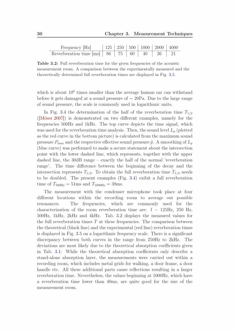
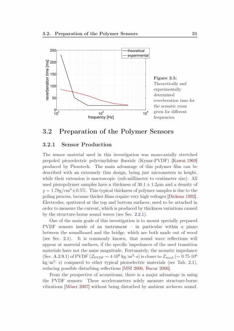
Frequency [Hz] 125 250 500 1000 2000 4000Reverberation time [ms] 86 75 60 40 26 21
Table 3.2: Full reverberation time for the given frequencies of the acoustic
measurement room. A comparison between the experimentally measured and the
theoretically determined full reverberation times are displayed in Fig. 3.5.
which is about 106 times smaller than the average human ear can withstandbefore it gets damaged at a sound pressure of ∼ 20Pa. Due to the large rangeof sound pressure, the scale is commonly used in logarithmic units.
In Fig. 3.4 the determination of the half of the reverberation time T1/2([Möser 2007]) is demonstrated on two different examples, namely for thefrequencies 500Hz and 1kHz. The top curve depicts the time signal, whichwas used for the reverberation time analysis. Then, the sound level Lp (plottedas the red curve in the bottom picture) is calculated from the maximum soundpressure Pmax and the respective effective sound pressure p. A smoothing of Lp
(blue curve) was performed to make a secure statement about the intersectionpoint with the lower dashed line, which represents, together with the upperdashed line, the 30dB range – exactly the half of the normal ’reverberationrange’. The time difference between the beginning of the decay and theintersection represents T1/2. To obtain the full reverberation time T1/2 needsto be doubled. The present examples (Fig. 3.4) exibit a full reverberationtime of T500Hz = 51ms and T1000Hz = 38ms.
The measurement with the condenser microphone took place at fourdifferent locations within the recording room to average out possibleresonances. The frequencies, which are commonly used for thecharacterization of the room reverberation time are: f = 125Hz, 250 Hz,500Hz, 1kHz, 2kHz and 4kHz. Tab. 3.2 displays the measured values forthe full reverberation times T at these frequencies. The comparison betweenthe theoretical (black line) and the experimental (red line) reverberation timesis displayed in Fig. 3.5 on a logarithmic frequency scale. There is a significantdiscrepancy between both curves in the range from 250Hz to 2kHz. Thedeviations are most likely due to the theoretical absorption coefficients givenin Tab. 3.1: While the theoretical absorption coefficients only describe astand-alone absorption layer, the measurements were carried out within arecording room, which includes metal grids for walking, a door frame, a doorhandle etc. All these additional parts cause reflections resulting in a largerreverberation time. Nevertheless, the values beginning at 1000Hz, which havea reverberation time lower than 40ms, are quite good for the size of themeasurement room.
3.2. Preparation of the Polymer Sensors 31
102
103
104
0
50
100
150
200
250
frequency [Hz]
reve
rbe
ratio
n t
ime
[m
s]
theoretical
experimental
Figure 3.5:
Theoretically and
experimentally
determined
reverberation time for
the acoustic room
given for different
frequencies.
3.2 Preparation of the Polymer Sensors
3.2.1 Sensor Production
The sensor material used in this investigation was mono-axially stretchedprepoled piezoelectric polyvinylidene fluoride (Kynar-PVDF) [Kawai 1969]produced by Piezotech. The main advantage of this polymer film can bedescribed with an extremely thin design, being just micrometers in height,while their extension is macroscopic (sub-millimeter to centimeter size). Allused piezopolymer samples have a thickness of 30.1± 1.2µm and a density of = 1.78g/cm3±0.5%. This typical thickness of polymer samples is due to thepoling process, because thicker films require very high voltages [Dickens 1992].Electrodes, sputtered at the top and bottom surfaces, need to be attached inorder to measure the current, which is produced by thickness variations causedby the structure-borne sound waves (see Sec. 2.2.1).
One of the main goals of this investigation is to mount specially preparedPVDF sensors inside of an instrument – in particular within a pianobetween the soundboard and the bridge, which are both made out of wood(see Sec. 2.1). It is commonly known, that sound wave reflections willappear at material surfaces, if the specific impedances of the used transitionmaterials have not the same magnitude. Fortunately, the acoustic impedance(Sec. A.2.9.1) of PVDF (ZPVDF ∼ 4·106 kg/m2· s) is closer to Zwood (∼ 0.75·106kg/m2· s) compared to other typical piezoelectric materials (see Tab. 2.1),reducing possible disturbing reflections [MSI 2006, Bucur 2006].
From the perspective of acousticans, there is a major advantage in usingthe PVDF sensors: These accelerometers solely measure structure-bornevibrations [Möser 2007] without being disturbed by ambient airborne sound.

32 Chapter 3. Measurement Techniques
Figure 3.6: Photo of the sputtering
device nicely showing the chromium
and gold targets.
Thus, they can be used for measurements in almost every environment, aslong as the measured setup is decoupled from structure surroundings, e.g. thebasement.
Sputtering Electrodes: Due to the piezoelectric effect (see Sec. 2.2.1),an external force will generate compensation charges, which appear on bothsurfaces of the thin polymer film. To detect these charges, thin metalelectrodes are attached on the top and bottom surfaces of the PVDF sensors.Sputtering thin metal films (chromium and gold) to the PVDF film is afast, easy and relatively inexpensive method of applying electrodes to asensor surface. The samples were sputtered with the Sputter Coater Emitech’K575XD’ (see Fig. 3.6) attaching a chromium and gold layer with an overallthickness of 56nm (chromium layer with 24nm and gold layer with 32nm).The chromium serves as a stabilizer for the final gold layer, rendering it moredurable on the piezopolymer film.
For the sensor design (sketch drawn in Fig. 3.7a), it needs to be taken intoaccount that the generated electric signal depends on the sputtered conductionlayer on the PVDF film. Only the ’both side sputtered area’ of the sensorfilm (the ’active recording’ area [MSI 2006]; marked by the slightly reddishsquare in Fig. 3.7a) will contribute to the measurement signal, if an externalvarying force is applied. Lacking a metal layer, the ’wings’ of the electrodesare not able to establish a clear electric field. Therefore, these areas will notsignificantly contribute to the overall signal. This has to be taken into account,when the film area is determined for the reconstruction of the external force.Another aspect of the actually used design was the relatively long distancebetween both electrode ’wings’. This certain form was choosen to reduce

3.2. Preparation of the Polymer Sensors 33
(a)
top electrode
PVDF filmactive recording area
bottom electrode
(b)
(c)
Figure 3.7: (a): Sketch of the specially designed PVDF sensors, which are used
for the Bechstein measurements, including the PVDF film as the basis and the top
and bottom electrodes (main recording area (reddish square) and the ’wings’).
Further descriptions in the text. (b): One side of the masked and already
sputtered PVDF film. (c): After removing the mask and cutting the PVDF sheet
closely to the gold electrodes.
distracting signal interactions between them.
In the next paragraph, it will be explained that the sensor structure wasnot clear from the beginning. Moreover, the current design was the result ofa long evolution. For a certain time, a completely different sensor design wasunder consideration, with the electrode ’wings’ on opposing sides (in contrastto only one side) to achieve an entirely symmetric arrangement. That way,possible signal perturbations between the electrode ’wings’ would be reducedto a minimum. But the design ends up in having the electrodes at one singleside due to constructional reasons, especially for the Bechstein measurements(see Sec 5.2). Of course, if one only has the intention to just place sensorsin the final constructed instrument, the symmetric arrangement would bethe perfect design, because the connection to the amplifier needs to be doneonly once. But the purpose of this investigation was always to determinethe differences in the sound-wave propagation depending on the constructionsteps and hence, the connections to the sensors needed to be removable allthe time.
During the sputtering process of the electrodes, specially cut masks needto be fixed on both sides of the sensor to produce a defined recording area[MSI 2006]. The usual mode of operation for the sputtering is as follows: i) cutmasks from polyethylene (PE ) pieces; ii) cut PVDF samples slightly smallerthan the masks, iii) glue them together, sandwiching the PVDF film between

34 Chapter 3. Measurement Techniques
the PE-masks; iv) afterwards, the chromium and gold layers are sputtered ontoboth sides (see Fig. 3.7b); v) removing carefully the masks from the PVDFfilm, avoiding short-circuits (top to bottom electrode) by damaging the fragilePVDF sensor; vi) the last step includes a final cut of the PVDF film closelyalong the electrodes without striking them (see Fig. 3.7c). This cut, whichwas also a recommendation from the piano makers, minimizes unnecessarysensor surface. The less film material is glued into the instrument, the betterthe investigation follows the minimal-invasive approach.
An example for a fully sputtered PVDF film is shown in Fig. 3.7c. Thesesensors are used for the Bechstein measurement program and have a recordingarea of about A = 3.6 · 10−5m2 and a side length of the main electrode areaof l = 0.006m.
3.2.2 Calibration & Characterization
The following calibration and characterization of the PVDF films are fullydescribed in [Kappel 2011] and below.
To use the PVDF sensors as measurement devices with a sufficientaccuracy, the calibration and the characterization were performed with respectto pivotal key parameters. There were calibration investigations towards thedependence of the piezoelectric coefficient2 on the initial pressure and thedynamical force amplitude. Also the long-term stability and the frequencyresponse, which is probably the most important parameter for acousticians,were documented for the characterization.
The data analysis throughout this investigation, comprising the whole dataprocessing and the respective plotting, was performed with ’matlab R2008a’[The MathWorks, Inc. ].
3.2.2.1 Setup
The direct piezoelectric effect (see Sec. 2.2.1) is defined as the response of thematerial to an external force [Mellinger 2003, Wada 1981]:
dij =
(
∂Di
∂σj
)
E
(3.4)
with D as the electric displacement, σ as the stress and the constant electricfield E; dij is the tensor describing the piezoelectric coefficient of the material.With D = Q/A and σ = F/A (with A describing the same area), Eq. 3.4 can
2PVDF has a negative d33 value, meaning that it will compress instead of expand
[Pu 2010]
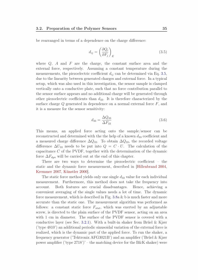
3.2. Preparation of the Polymer Sensors 35
be rearranged in terms of a dependence on the charge difference:
dij =
(
∂Qi
∂Fj
)
E
(3.5)
where Q, A and F are the charge, the constant surface area and theexternal force, respectively. Assuming a constant temperature during themeasurements, the piezoelectric coefficient dij can be determined via Eq. 3.5,due to the linearity between generated charges and external force. In a typicalsetup, which was also used in this investigation, the sensor sample is clampedvertically onto a conductive plate, such that no force contribution parallel tothe sensor surface appears and no additional charge will be generated throughother piezoelectric coefficients than d33. It is therefore characterized by thesurface charge Q generated in dependence on a normal external force F , andit is a measure for the sensor sensitivity:
d33 =∆Q33
∆F33
(3.6)
This means, an applied force acting onto the sample/sensor can bereconstructed and determined with the the help of a known d33 coefficient anda measured charge difference ∆Q33. To obtain ∆Q33, the recorded voltagedifference ∆U33 needs to be put into Q = C · U . The calculation of thecapacitance C of the PVDF, together with the determination of the dynamicforce ∆Fdyn will be carried out at the end of this chapter.
There are two ways to determine the piezoelectric coefficient – thestatic and the dynamic force measurement, described in [Hillenbrand 2004,Kremmer 2007, Künstler 2000].
The static force method yields only one single d33 value for each individualmeasurement. Furthermore, this method does not take the frequency intoaccount. Both features are crucial disadvantages. Hence, achieving aconvenient averaging of the single values needs a lot of time. The dynamicforce measurement, which is described in Fig. 3.8a & b is much faster and moreaccurate than the static one. The measurement algorithm was performed asfollows: a constant static force Fstat, which was exerted by an adjustablescrew, is directed to the plain surface of the PVDF sensor, acting on an areawith 1 cm in diameter. The surface of the PVDF sensor is covered with aconductive layer (see Sec. 3.2.1). With a built-in shaker from Brüel & Kjær(’type 4810’) an additional periodic sinusoidal variation of the external force isrealized, which is the dynamic part of the applied force. To run the shaker, afrequency generator (’Tektronix AFG3021B’) and an amplifier (’Brüel & Kjærpower amplifier (’type 2718’)’ – the matching device for the B&K shaker) were

36 Chapter 3. Measurement Techniques
shaker
force sensor
generatorfunction−
oscilloscope
amplifier
amplifier
amplifier
voltage−PVDF sensor
PC
0 0.5 1 1.5 2
−2
0
2
4
6
dynam
ic forc
e [N
]
time [s]
−20
−10
0
10
20
30
40
50
60
ch
arg
e [
pC
]−20 −10 0 10 20
−1
0
1
2
charge [pC]
dyn. fo
rce [N
](a)
(b)
(c)
PPP
PPP
PPP
Figure 3.8: (a): Picture of the dynamical d33 measurement setup. (b): Dynamic
force configuration for determing the d33 coefficient: With a constant initial
pressure, a periodic sinusoidal force (produced by the shaker Brüel & Kjær (’type
4810’)) generates a periodic electrical signal. Both signals are measured and
analyzed by an oscilloscope, which plots the two parameters against each other.
The resulting regression line gives a slope, being exactly d33 (see Eq. 3.9). (c):
Measured charge [pC] and force [N] captured with the dynamic force method in
the big frame. The determination of d33 by averaging with a regression line in the
inset frame. d33 = 13.5pC/N for this example.
included in the measurement setup. The force is recorded by the force sensor’Burster – type 8435’, which is located right below the PVDF sensor.
The overall, time-dependent applied force can be expressed by:
Fdyn = Famp · cos(2πft) + Fstat (3.7)
Through the dynamic part of the force, the polarization of the piezoelectricpolymer film is varying. This polarization change induces the generation of
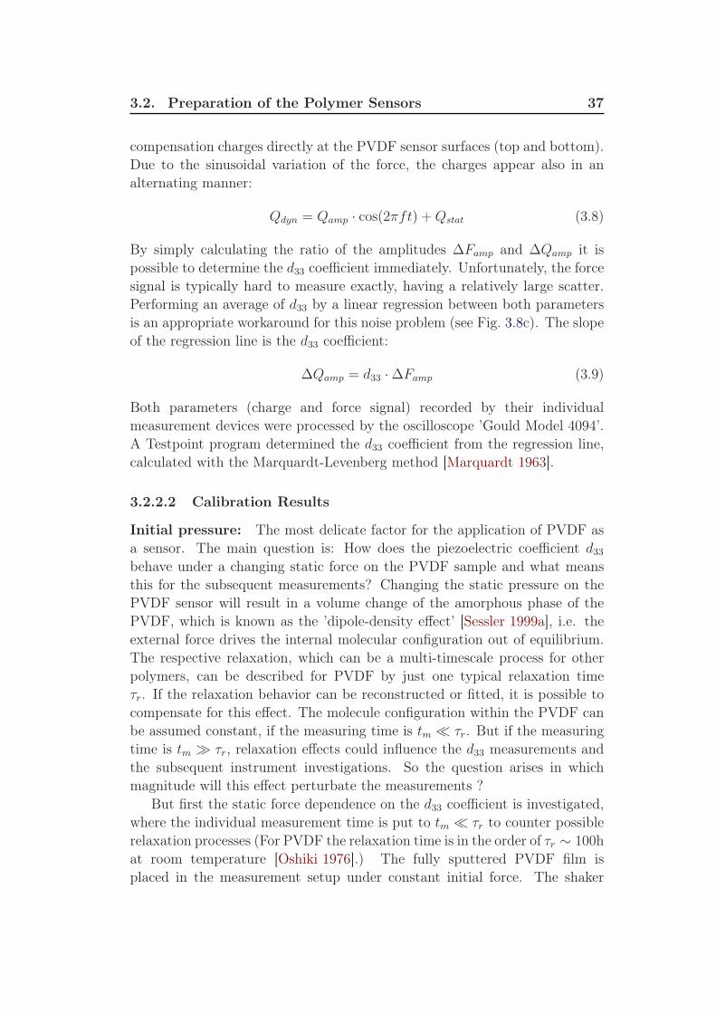
3.2. Preparation of the Polymer Sensors 37
compensation charges directly at the PVDF sensor surfaces (top and bottom).Due to the sinusoidal variation of the force, the charges appear also in analternating manner:
Qdyn = Qamp · cos(2πft) +Qstat (3.8)
By simply calculating the ratio of the amplitudes ∆Famp and ∆Qamp it ispossible to determine the d33 coefficient immediately. Unfortunately, the forcesignal is typically hard to measure exactly, having a relatively large scatter.Performing an average of d33 by a linear regression between both parametersis an appropriate workaround for this noise problem (see Fig. 3.8c). The slopeof the regression line is the d33 coefficient:
∆Qamp = d33 ·∆Famp (3.9)
Both parameters (charge and force signal) recorded by their individualmeasurement devices were processed by the oscilloscope ’Gould Model 4094’.A Testpoint program determined the d33 coefficient from the regression line,calculated with the Marquardt-Levenberg method [Marquardt 1963].
3.2.2.2 Calibration Results
Initial pressure: The most delicate factor for the application of PVDF asa sensor. The main question is: How does the piezoelectric coefficient d33behave under a changing static force on the PVDF sample and what meansthis for the subsequent measurements? Changing the static pressure on thePVDF sensor will result in a volume change of the amorphous phase of thePVDF, which is known as the ’dipole-density effect’ [Sessler 1999a], i.e. theexternal force drives the internal molecular configuration out of equilibrium.The respective relaxation, which can be a multi-timescale process for otherpolymers, can be described for PVDF by just one typical relaxation timeτr. If the relaxation behavior can be reconstructed or fitted, it is possible tocompensate for this effect. The molecule configuration within the PVDF canbe assumed constant, if the measuring time is tm ≪ τr. But if the measuringtime is tm ≫ τr, relaxation effects could influence the d33 measurements andthe subsequent instrument investigations. So the question arises in whichmagnitude will this effect perturbate the measurements ?
But first the static force dependence on the d33 coefficient is investigated,where the individual measurement time is put to tm ≪ τr to counter possiblerelaxation processes (For PVDF the relaxation time is in the order of τr ∼ 100hat room temperature [Oshiki 1976].) The fully sputtered PVDF film isplaced in the measurement setup under constant initial force. The shaker

38 Chapter 3. Measurement Techniques
2 4 6 8 10 12 1412
13
14
15
16
17
18
static force [N]
d33−
coeffic
ient [p
C/N
]
PVDF sensor 1
PVDF sensor 2
1 2 3 4 5 610
10.5
11
11.5
12
12.5
13
13.5
14
14.5
force amplitude (peak−to−peak) [N]
d33−
coeffic
ient [p
C/N
]
sensor 1 time 1
sensor 1 time 2
sensor 1 time 3
sensor 2 time 1
sensor 2 time 2
sensor 2 time 3
linear regression
(a) (b)
Figure 3.9: (a): d33 coefficient hysteresis loop over the static force Fstat. The
amplitude of the dynamic force was constant at 2N ± 0.1N (peak-to-peak).
Indicated by the arrows, the increasing and decreasing of Fstat is documented.
(b): d33 coefficient vs. the dynamic force amplitude, where the static force was
held constant at 6N ± 0.1N. Three independent measurements are obtained for
each investigated sample at different times (black curves). The d33 behavior can be
assumed as linear, indicated by the red regression lines, over this amplitude range.
For both samples the same slope m ∼ (0.15± 0.016)pC/N2 was measured,
justifying the linear regression.
generates a sinusoidal varying dynamic force Famp · cos(2πft) additionallyto the static force Fstat (see Eq. 3.7), which is produced by the adjustablescrew. The resulting varying electric signal, recorded by an oscilloscope, isfurther processed by a computer, which determines the regression line betweenboth parameters and the subsequently resulting slope – the d33 coefficient.To obtain an appropriate averaging, for each initial pressure value severalmeasurements are carried out and the d33 coefficient is determined. The d33outcome for the investigated sensors, shown in Fig. 3.9a, follows a hysteresisloop for increasing and decreasing static force, which is indicated by theinserted arrows. The amplitude of the dynamic part of the force is set toa constant value of 2N ± 0.1N (peak-to-peak). Initially, from 1N to 4N, theconnection to the force sensor is not ideal by reason of a relatively largedynamic part of the force compared to the static force. This effect generatesa ’threshold force’ actually only for these measurements, where the measuredforce value is too small. Hence, a too high d33 value is determined in thisrange as a consequence.
Using exactly this data acquisition setup, this threshold effect becomesminimal in the range from 4N to 11N, indicated by the relatively constantd33 behavior. Unfortunately, the used measurement setup is only designed forstatic forces up to 11N. Any forces beyond that point will affect the accuracy

3.2. Preparation of the Polymer Sensors 39
of the recording setup, especially the B&K shaker. That could result in a toohigh piezoelectric coefficient (as seen also in Fig. 3.9a for static force valuesbeyond 11N), when the static force is not properly transfered to the forcesensor. When the force is slowly released, the existing polymer configurationtemporarily stays this way and begins to relax to its initial state. This willalso end up in a seemingly higher d33 coefficient (see also Fig. 3.9a).
All investigated PVDF samples show exactly the same behavior, buton different initial levels. For each sensor, which will be used for furthermeasurements, a separate d33 determination has to be made. The observeddeviation in the piezoelectric coefficient can be explained by fluctuationswithin the polymer material and also by the size variation of the sputteredelectrodes, caused during the sputtering process by the attached masks[Kappel 2011].
Excitation amplitude: An additional important parameter is the d33dependence on the excitation force amplitude. During these measurements,the static force was held at 6N ± 0.1N. Shown exemplarily in Fig. 3.9b, twoPVDF samples were independently analyzed at three different times. Theirbehavior can be appropriately described by a linear correlation, shown asthe red lines. Both PVDF sensors have the same slope of m ≈ (0.15 ±0.016)pC/N2.
Signal-to-Noise Ratio: The signal-to-noise ratio (S/N ratio)[Guillaume 2006] was determined with the help of strings mounted onto themultichord and measuring the first harmonic of a tone with the fundamentalfrequency of fS/N = 200Hz. The observed piezopolymer S/N ratio at thisfrequency is Lp = 78dB, representing a good S/N ratio.
3.2.2.3 Other notable parameters
Temperature and Humidity: The temperature variations within a singlemeasurement run are not significant and are all in the range of one ortwo degree Celsius. The maximum temperature range considering severalweeks did not extend below 20C and above than 28C. Exemplarily shownin Fig. 3.10b during the d33 long-term measurement, the temperature wasmonitored over the whole time range. It has been found that the variabilityof the temperature is rather small and has no significant correlation (see A.2.2)with the d33 coefficient behavior (Ctemp = 0.016).
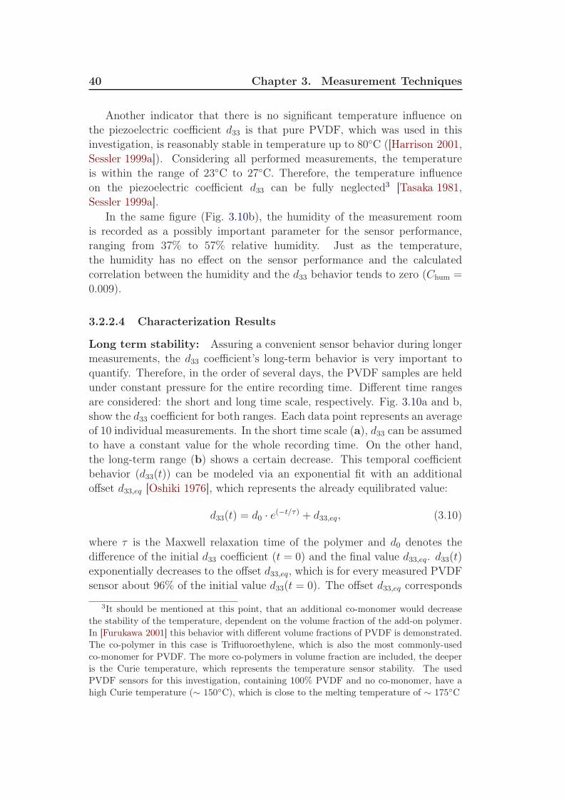
40 Chapter 3. Measurement Techniques
Another indicator that there is no significant temperature influence onthe piezoelectric coefficient d33 is that pure PVDF, which was used in thisinvestigation, is reasonably stable in temperature up to 80C ([Harrison 2001,Sessler 1999a]). Considering all performed measurements, the temperatureis within the range of 23C to 27C. Therefore, the temperature influenceon the piezoelectric coefficient d33 can be fully neglected3 [Tasaka 1981,Sessler 1999a].
In the same figure (Fig. 3.10b), the humidity of the measurement roomis recorded as a possibly important parameter for the sensor performance,ranging from 37% to 57% relative humidity. Just as the temperature,the humidity has no effect on the sensor performance and the calculatedcorrelation between the humidity and the d33 behavior tends to zero (Chum =
0.009).
3.2.2.4 Characterization Results
Long term stability: Assuring a convenient sensor behavior during longermeasurements, the d33 coefficient’s long-term behavior is very important toquantify. Therefore, in the order of several days, the PVDF samples are heldunder constant pressure for the entire recording time. Different time rangesare considered: the short and long time scale, respectively. Fig. 3.10a and b,show the d33 coefficient for both ranges. Each data point represents an averageof 10 individual measurements. In the short time scale (a), d33 can be assumedto have a constant value for the whole recording time. On the other hand,the long-term range (b) shows a certain decrease. This temporal coefficientbehavior (d33(t)) can be modeled via an exponential fit with an additionaloffset d33,eq [Oshiki 1976], which represents the already equilibrated value:
d33(t) = d0 · e(−t/τ) + d33,eq, (3.10)
where τ is the Maxwell relaxation time of the polymer and d0 denotes thedifference of the initial d33 coefficient (t = 0) and the final value d33,eq. d33(t)exponentially decreases to the offset d33,eq, which is for every measured PVDFsensor about 96% of the initial value d33(t = 0). The offset d33,eq corresponds
3It should be mentioned at this point, that an additional co-monomer would decrease
the stability of the temperature, dependent on the volume fraction of the add-on polymer.
In [Furukawa 2001] this behavior with different volume fractions of PVDF is demonstrated.
The co-polymer in this case is Trifluoroethylene, which is also the most commonly-used
co-monomer for PVDF. The more co-polymers in volume fraction are included, the deeper
is the Curie temperature, which represents the temperature sensor stability. The used
PVDF sensors for this investigation, containing 100% PVDF and no co-monomer, have a
high Curie temperature (∼ 150C), which is close to the melting temperature of ∼ 175C

3.2. Preparation of the Polymer Sensors 41
0 5 10 15 20 25 3012
13
14
15
16
17
time [min]
d33−
coeffic
ient [p
C/N
]
13
14
15
16
17
d3
3−
co
eff
icie
nt
[pC
/N]
sensor 1 (fit)
sensor 2 (fit)
0 50 100 150 200
40
50
60
Hu
mid
ity [
% R
s]
time [h]
24
26
28
Te
mp
era
ture
[C
els
ius]
(a) (b)
Figure 3.10: (a): d33 coefficient over a short time range. Several measurements
of two sensors are included in this plot and show a significantly flat d33 behavior
over 30 minutes.
(b): A longer time range (up to 235 hours) for the d33 coefficient evolution in the
upper plot. Fitted with d33(t) = d0 ∗ exp (−t/τ) + d33,eq both curves are slightly
decreasing towards the equilibrated value d33,eq. Supplemental, the evolution of
humidity (black) and temperature (red) are observed in the lower frame during the
sensor 1 measurements. The calculated correlations of these parameters with the
d33 evolution give values of Chum = 0.009 for the humidity and Ctemp = 0.016 for
the temperature. Hence, no significant correlation has been found.
to the already relaxed molecule configuration; the relaxation time τ for bothplotted curves (see Fig. 3.10b) have a value of τ ≈ 77h, which is in goodagreement with [Oshiki 1976], who finds a value of about τ ∼ 100h for roomtemperature. For the investigated PVDF sensors 1 and 2, the equilibratedpiezoelectric coefficients are d33,eq1 = 13.2pC/N and d33,eq2 = 15.5pC/N,respectively. During these measurements, the values for temperature andhumidity are simultaneously recorded and have already been discussed inSec. 3.2.2.3.
Taking into account that the investigation on the instruments includemeasurements, which last only few minutes at maximum, it is possibleto conclude, that the d33 coefficient is constant during one recording.Furthermore, assuring a mounting of the PVDF sensors at least some daysbefore the actual measurements begin, the coefficient behavior can also beassumed constant after this time. Even a data acquisition having the finalvalue of the d33,eq coefficient, gives only a decrease of 4%, which is sufficientlysmall.
Frequency response: Fig. 3.11 describes two different measurementmethods to investigate the frequency response of the PVDF sensors. The
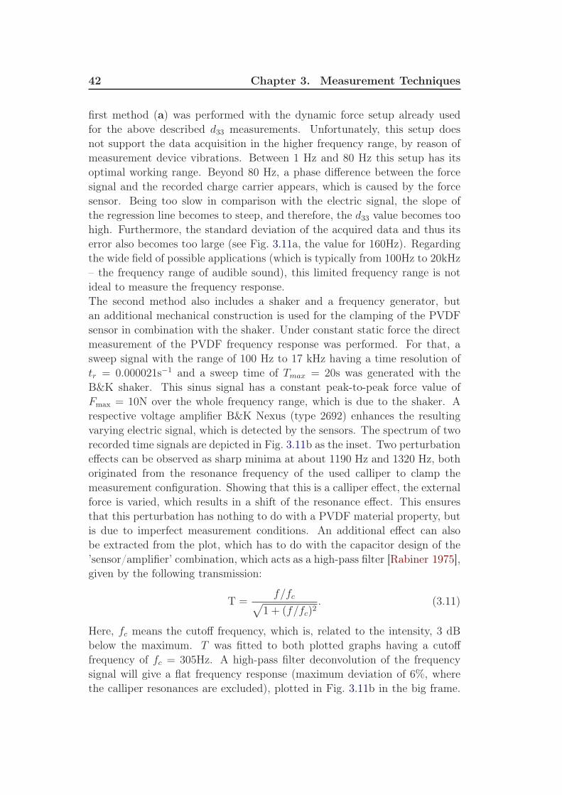
42 Chapter 3. Measurement Techniques
first method (a) was performed with the dynamic force setup already usedfor the above described d33 measurements. Unfortunately, this setup doesnot support the data acquisition in the higher frequency range, by reason ofmeasurement device vibrations. Between 1 Hz and 80 Hz this setup has itsoptimal working range. Beyond 80 Hz, a phase difference between the forcesignal and the recorded charge carrier appears, which is caused by the forcesensor. Being too slow in comparison with the electric signal, the slope ofthe regression line becomes to steep, and therefore, the d33 value becomes toohigh. Furthermore, the standard deviation of the acquired data and thus itserror also becomes too large (see Fig. 3.11a, the value for 160Hz). Regardingthe wide field of possible applications (which is typically from 100Hz to 20kHz– the frequency range of audible sound), this limited frequency range is notideal to measure the frequency response.The second method also includes a shaker and a frequency generator, butan additional mechanical construction is used for the clamping of the PVDFsensor in combination with the shaker. Under constant static force the directmeasurement of the PVDF frequency response was performed. For that, asweep signal with the range of 100 Hz to 17 kHz having a time resolution oftr = 0.000021s−1 and a sweep time of Tmax = 20s was generated with theB&K shaker. This sinus signal has a constant peak-to-peak force value ofFmax = 10N over the whole frequency range, which is due to the shaker. Arespective voltage amplifier B&K Nexus (type 2692) enhances the resultingvarying electric signal, which is detected by the sensors. The spectrum of tworecorded time signals are depicted in Fig. 3.11b as the inset. Two perturbationeffects can be observed as sharp minima at about 1190 Hz and 1320 Hz, bothoriginated from the resonance frequency of the used calliper to clamp themeasurement configuration. Showing that this is a calliper effect, the externalforce is varied, which results in a shift of the resonance effect. This ensuresthat this perturbation has nothing to do with a PVDF material property, butis due to imperfect measurement conditions. An additional effect can alsobe extracted from the plot, which has to do with the capacitor design of the’sensor/amplifier’ combination, which acts as a high-pass filter [Rabiner 1975],given by the following transmission:
T =f/fc
√
1 + (f/fc)2. (3.11)
Here, fc means the cutoff frequency, which is, related to the intensity, 3 dBbelow the maximum. T was fitted to both plotted graphs having a cutofffrequency of fc = 305Hz. A high-pass filter deconvolution of the frequencysignal will give a flat frequency response (maximum deviation of 6%, wherethe calliper resonances are excluded), plotted in Fig. 3.11b in the big frame.

3.2. Preparation of the Polymer Sensors 43
100
101
102
12
12.5
13
13.5
14
14.5
15
frequency [Hz]
d33−
coeffic
ient [p
C/N
]
102
103
104
0.5
1
1.5
2
2.5
frequency [Hz]
response function
102
103
104
frequency [Hz]
(a) (b)
Figure 3.11: (a): Measured frequency response gathered with the dynamic force
measurement setup (see Fig. 3.8). Not ideal for a broad frequency range, but
sufficient for 1 Hz to 80 Hz.
(b): Alternative method to check the independence of d33 from the frequency by
measuring the resulting PVDF response function of a sweep from 100Hz to 17
kHz. A high pass effect occurs for the original data (see the inset), which can be
modeled with the red graph (see Eq. 3.11). A deconvolution by this effect yields a
flat PVDF frequency response function (bigger graph).
All subsequent PVDF recording signals are corrected for this high-pass effect.
Usually a further important parameter would be the thickness extensionresonance spectrum of the polymer film, in particular the superelevation atthe resonance frequency. But considering a thickness of about 30µm, and thesound wave velocity within PVDF of vPVDF = 2.3km/s the lowest resonancefrequency can be determined by:
fr =vPVDF
2 · dfilm(3.12)
which comes from the condition that half of the wavelength of thestructure-borne sound wave fits exactly to the thickness of the PVDF film.This yields a lower-limit resonance frequency of about fr = 37MHz, farbeyond the parameter range in this investigation with a maximum of 20 kHz.Therefore, all measurements are located completely within the constant rangeof the mechanical resonance spectrum (see Appendix A.2.6 and [Möser 2010]).
Additionally, the piezoelectric resonance effect [Mellinger 2003] should benoted here, although its resonance frequency is even larger compared to themechanical resonance. For corona charged PVDF with a thickness of 24 µm,a piezoelectric resonance of about 50 MHz was found [Kulek 2002], which isalso far beyond the audible range.

44 Chapter 3. Measurement Techniques
parameter value [unit] commentε0 8.86 · 10−12 As/Vm physical constantεr ∼ 9 relative permittivity for
β-PVDF ([Hahn 1985])A 3.6 · 10−5 m2 (Bechstein) active surface area of PVDF
1.69 · 10−4 m2 (Multichord) sensor (±30% [Kappel 2011])d33 (14± 0.5) · 10−12 C/N measured piezoelectric constantd (30.1± 1.2) · 10−6 m thickness PVDF film
Table 3.3: Listed values, either calculated or constant, for the determination of
the external dynamic force routed to the surface of the PVDF film.
3.2.3 External Dynamic Force
Having done the complete characterization and calibration of the PVDFsensors, the calculation of a dynamic part of the external force acting onthe sensor plane can be determined. By configuration, there is no forcecontribution of a static part within the measurement signal. Certainly,this particular characteristic qualifies these thin polymer sensors as a dataacquisition device for sound vibrations. The knowledge of relation Eq. 3.9and the behavior of the piezoelectric coefficient for the investigated sensorsgives the possibility of the direct determination of the dynamic part of theexternal force, where Eq. 3.9 marks the starting point:
∆Qdyn = d33 ·∆Fdyn (3.13)
Due to the fact, that eventually a voltage U , generated by the PVDF film, ismeasured, the well known relation Q = C · U will be further used. The twosputtered electrodes, which encase the dielectric PVDF, represent a capacitorwith the respective capacitance C:
C = ε0 · εr ·A
d(3.14)
at which A is the area with the acting force (see 3.2.1) of the gold sputteredpolymer, d the film thickness, ε0 the vacuum permittivity and εr the relativepermittivity. The three formulas in combination yield an expression, which ispractical for the measurement analysis:
∆Fdyn = ε0 · εr ·A
d33 · d·∆U (3.15)
The values for the polymer accelerometers are listed in table Tab. 3.3.With Eq. 3.15, the absolute value of the dynamic force can be calculated.
All the following instrument measurements, recorded by the PVDF sensors,
3.3. Condenser Microphones 45
are calibrated in this way providing the result in units of Newton [N]. A typicalvalue for this investigation is FBechst. ∼ 0.3N (Fig. 5.7) for the Bechsteinmeasurements and FMultich. ∼ 1.5N for the multichord recordings. Theobvious difference in the dynamic force is solely due to the different areascovered by the mounted bridges. For the multichord, the covered area of thebridge is smaller and due to the same excitation mechanism for both recordingseries, the dynamic force is therefore larger than in the Bechstein case.
3.3 Condenser Microphones
Since there is an extensive use of microphones in the present investigation,in particular capacitor microphones ([Eargle 2004, Ballou 2009, Wong 1997]),a description of the most important features is justified. But as acommon standard technique, where the characteristics are completelyknown and provided by the microphone manufacturer Brüel & Kjær, thedocumentation about the functionality and the characteristics are providedin the appendix A.1.1.
3.4 Chapter Conclusion
The first part of this chapter introduces the acoustic characterization of theanechoic chamber in terms of dimension, absorption, soundproofing, andreverberation time. Knowing these parameters will yield reliable and secureairborne measurements within the recording room, which have been takenplace for the multichord investigation described in the next chapter.
It was also demonstrated above that carefully prepared piezoelectricpolymer sensors (which are produced from mono-axially stretched PVDF inthis case) can be used as integrated force sensors to record body vibrationswith minimal invasion of the investigated system. This recording procedureapplies to many vibrational systems, such as the monitoring of buildings,vehicles, machinery, alarm systems, etc. There are enormous advantages inusing these polymer materials: namely their relatively low cost and theirminimal dimensions so that they can be used in large quantity withoutdisturbing the monitored system.
Despite having many advantages, one fundamental challenge withpolymers is their relaxation under external stress. Therefore, it is extremelyimportant to understand and characterize the sensor response on short andlong time scales. It was demonstrated that a careful calibration will takeinto account a slow drift of parameters. The piezoelectric coefficient d33,representing the vertical electromechanical conversion, was determined with

46 Chapter 3. Measurement Techniques
respect to the following crucial parameters: initial force Fstat, amplitude of thedynamical force Fdyn, frequency response, and long-term stability. The exactknowledge of the sensor behavior under specific parameter variations providesthe possibility of a secured and calibrated body-vibration measurement, whichis shown in the next two chapters. Along with the airborne measurementsof a conventional condenser microphone, statements can be made about thevibrational energy distribution during the excitation of the system.

Chapter 4
Multichord as a Conceptional
Soundboard
The basic theory for some of the acoustic effects occuring in the soundgeneration of solid-state vibrations and the emerging dispersion relation wasprovided by the LCM model in chapter 2.1.4. A further evolution of thismodel towards an underlying obstacle pattern for the propagating material isprovided in the first section.
The investigation of these theoretical effects is difficult when theparticularly shaped sound board of an upright piano or even grand piano isconsidered – the eigenmodes heavily depend on the specific shape. However,a surface structured with regular ribs can be mapped to the soundboard.Therefore, it was decided to build a dedicated setup by a rectangularmultichord, which is easily understood, cheap and well controllable. Thismultichord can be adopted as a simplified piano model and to render itas similar as possible to a real piano, the instrument will be equippedwith all neccessary genuine parts important for the spectral radiation of theboard. The spectral change of the propagating sound waves in the board (seeadditionally [Kappel 2010] for the multichord investigations) is measured bymeans of condensor microphones and state-of-the-art piezopolymer sensors,described in detail in [Kappel 2011] and in chapter 3.2.
The chapter goes on with the explanation of the construction, geometryand measurement setup of the multichord in Sec. 4.2. In Sec. 4.3, the acquireddata and the respective results are presented. Finally, in Sec. 4.3.3, the datais fitted to the above-mentioned adjusted LCM model and discussed in detail.
4.1 LCM Model Projection to the Ribbed
Soundboard
The LCM model (see Sec. 2.1.4) will be further developed and described inthis section. This advancement of the model describes the structure-bornesound-wave propagation through a patterned material. This materialshould be infinitely extended towards one direction, assuming an asymptotic

48 Chapter 4. Multichord as a Conceptional Soundboard
situation. The bonding of the material is arranged in a row. This, in principle,can be summed up to a simplification as a quasi-1D system with unit cells(ribs with distance a) starting an infinite series with a periodic boundarycondition. The next step in the model is a sound wave scattered forward andbackward by the first obstacle (the first rib). This scattering process dependson the relative phase of the incoming wave and its wavelength, of course. Thesecond rib will do the same, and so on.
Now consider a non-infinite series by a further evolution of the modelto fit better the reality: a finite number of ribs (N + 1) shall be infinitelyheavy and infinitely thin, while the soundboard has a finite size of N · a.Solving the model with the given boundary conditions yields standing waveswith a wavelength given by the constraint λn = 2a/n, where n is a positiveinteger. These conditions describe obviously the only solution for thissystem. Furthermore, N -fold degenerate respective frequencies for an elasticmembrane with νn = c(ν)/λn are introduced, where c(ν) represents the speedof sound in dependence of the wavelength.
To advance the model, the weight of the ribs remains large but finite,which results in a coupling between the former independent individualinter-rib sections, described by a coupling constant ε. This also yields aremoval of the former degeneration and consequently the frequency spectrumwill consist of N separate eigenfrequencies having a band width of 2ε
and located at the harmonics for the elastic membrane νn. Hence, anadaption was realized from an extended system including elasticity to aset of coupled oscillators with frequencies νn. Following the LCM model[Ashcroft 1976, Morse 1987, Ziman 1972, Kittel 1953], the equation of motion(including the harmonics of the elastic membrane νn) can be written down as:
uj = −ν2n + ε(uj+1 − 2uj + uj−1) (4.1)
with integer j = 1, . . . , N and u representing the displacement. Again, thecoupling is restricted to the nearest neighbors only and the speed of soundis neglected. With the ansatz uj ∼ eikjj/N , kj = 2π/λj and the periodicboundary condition u([N + 1] · a) = u(a); u(0) = u(N · a), the frequencyspectrum will include allowed ’pass bands’:
νj = ± νn ± 2ε sin(kj/(2N)) (4.2)
In essence, located at each resonance frequency νn of the soundboard, astructure of ’pass-band’ frequencies emerges, given by the dispersion relationin Eq. 2.7. Changing the boundary conditions to a fixed one would yieldfrequencies only shifted within the ’pass band’. Therefore, the result remainsthe same qualitatively.
4.1. LCM Model Projection to the Ribbed Soundboard 49
The rib distance or the coupling could easily be varied by changing therespective entries of the parameters νn or ε. Theoretically, this would resultin a shift of the individual frequencies in the ’band pass’. Even the completedestruction of the band structure can be achieved through a fully disorderedsystem [Condat 1986, Crisanti 1993, Bayer 1993].
Since this configuration is fully symmetric, as shown by Eq. 4.2, theabove-explained situation is clearly valid for positive and negative frequencies.Even though the negative frequencies are solutions to Eq. 4.2, they do not haveany meaning in reality. This effect is linear and holds for any coupling. Withan increase of the coupling factor, the sharpness of the peaks in the frequencyspectrum will decrease, while the overlap of the sound waves between theinter-rib distances increases.
In the following, the limits of the model are discussed: The multichordused in the experiment has a finite length, thus imposing fixed boundaryconditions. The finite size and mass of the ribs, the change in cross section ofthe soundboard, as well as the material imperfections, lead to deviations of thefrequency response from the the above-discussed adjusted LCM model. Thequestion arises, what are the observable effects in the spectrum concerningthese imperfections? At least, one can expect a strong damping of frequenciesin the spectrum, which means that these sound waves are not allowed topropagate through the material limited by the rib distances. They are reflectedby the rib (acting as the scatterer) in such a way that the incoming waveinterferes destructively with the reflected wave. As a result, large regions inthe spectrum should be damped and bands of allowed frequencies – the ’passbands’ – should be observed, approximately within the intervals [±νn; ±νn±2ε].
The specific eigenmodes of the studied multichord should be mentionedhere as a short preview on the special structure of the investigated instrument(see Sec. 4.3). The two most important ones are LSB, which is the firstlongitudinal mode and corresponds to the major part of the soundboardlength, and LBR, which is the second one in longitudinal direction and ismarked by the distance between the excitation bridge and the end of thesoundboard (see Fig. 4.6; see Fig. 4.2 for a complete description of themultichord dimension). Therefore, any generated spectral feature from thescattering could only appear on top of existing resonances νSB and νRB ofthe unperturbated (i.e. rib-free) resonance board. What actually can beexpected from the measurements are peaks with respective band structureat about ν0,long ≃ c/(2LSB) and ν0,long ≃ c/2LBR including all of theirharmonics. Again, the configuration is fully symmetric, including left and
right propagating sound waves. Hence, the banded scattering structure on the’positive’ side of the respective resonances νSR,n is completely mirrored on the

50 Chapter 4. Multichord as a Conceptional Soundboard
’negative’ side of νSR,n. That can be expressed with νSR,n ± νk, k = 1, ..., N .This is exactly the spectral behavior that will be described in the resultssection.
There is an alternative perspective of the theoretical explaination of thiseffect. So far, the board with infinite-mass ribs (ε = 0) is the starting point ofthe consideration. Then, ε becomes small, allowing to emerge the ’pass band’effects in the frequency spectrum. The alternative view comprises a situation,which is closer to the experiment. Assume an unperturbated board with nospecific modes and where the correlation is ε = ∞. For an increasing numberof attached ribs, the unperturbated modes, which are the allowed resonancesadditionally to the main board resonances, begin to emerge. This descriptionis closer to the experimental situation due to the subsequent mounting of theribs, and perfectly analogous to the picture above. Both considerations resultin a band of natural symmetric eigenfrequencies on top of the fundamentalresonances due to the dimensions of the soundboard.
4.2 Construction & Experimental Setup
The multichord, intended as a conceptional soundboard, was constructed forseveral reasons. On the one hand, it is possible to test the newly calibrated& characterized PVDF sensors (see Sec. 3.2.2) on a ’real’ vibrating andsound-radiating object and on the other hand to optimize the procedure.With the multichord recording experiences, the handling of the sensors,mounted in a genuine piano (see Sec. 5) becomes easier and more familiar.Nevertheless, a multichord is a stand-alone instrument worth to investigatepossibly occuring physical effects. Due to the simplified geometry, whichhas significant difference to a real piano, scattering effects should be on adifferent level compared to the piano setup, which is much more complex.To investigate the unique sound-wave propagation characteristics betweenboth vibrating constructions and even differences between certain constructionsteps is one of the major aims. The main objective is the investigation ofthe spectral characteristics of the sound propagated in and radiated from asoundboard with mounted ribs.
A rectangular multichord (1.2 m x 0.28 m) fully equipped with boundarybridges (for a defined length of the strings), the excitation bridge, tuningpegs and piano strings was constructed (see Fig. 4.1). Commercially availablewood glue was used for the adhesive bonding of the individual parts. Thisis quite common even for real pianos. Ribs are significant for the pianoand its sound radiation (discussed in 2.1.3). A number of equidistant ribs(seen also in Fig. 4.2) was successively placed under the soundboard. After
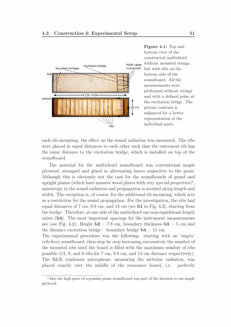
4.2. Construction & Experimental Setup 51
Figure 4.1: Top and
bottom view of the
constructed multichord
without mounted strings,
but with ribs on the
bottom side of the
soundboard. All the
measurements were
performed without strings
and with a defined pulse at
the excitation bridge. The
picture contrast is
enhanced for a better
representation of the
individual parts.
each rib mounting, the effect on the sound radiation was measured. The ribswere placed in equal distances to each other such that the outermost rib hasthe same distance to the excitation bridge, which is installed on top of thesoundboard.
The material for the multichord soundboard was conventional mapleplywood, arranged and glued in alternating layers respective to the grain.Although this is obviously not the case for the soundboards of grand andupright pianos (which have massive wood plates with very special properties)1,anisotropy in the sound radiation and propagation is avoided along length andwidth. The exception is, of course, for the additional rib mounting, which actsas a restriction for the sound propagation. For the investigation, the ribs hadequal distances of 7 cm, 9.8 cm, and 14 cm (see b1 in Fig. 4.2), starting fromthe bridge. Therefore, at one side of the multichord one non-equidistant lengthexists (b4). The most important spacings for the instrument measurementsare (see Fig. 4.2): Height b2 = 7.8 cm, boundary thickness b3 = 5 cm andthe distance excitation bridge – boundary bridge b4 = 11 cm.The experimental procedure was the following: starting with an ’empty’(rib-free) soundboard; then step by step increasing successively the number ofthe mounted ribs until the board is filled with the maximum number of ribspossible (13, 9, and 6 ribs for 7 cm, 9.8 cm, and 14 cm distance respectively).The B&K condenser microphone, measuring the airborne radiation, wasplaced exactly over the middle of the resonance board, i.e. perfectly
1Also the high price of a genuine piano soundboard was part of the decision to use maple
plywood.

52 Chapter 4. Multichord as a Conceptional Soundboard
Figure 4.2: Overview of the multichord setup with mounted ribs (b1 represents
the distance between ribs). The hammering device is sketched on the right-hand
side and excites the resonance board via the sound bridge with a single pulse. The
airborne soundwaves were recorded by a B&K condensor microphone right above
the arrangement and by PVDF piezopolymer sensors glued between the bridge and
the board. Further dimensions are: height b2 = 7.8 cm, boundary thickness b3 =
5 cm and distance from excitement bridge to boundary bridge, b4 = 11 cm.
perpendicular to the board’s surface2. This microphone location provides thecomplete soundboard radiation (see Sec. A.2.8), because the radiation of aboard has a specific characteristic – a dipole radiation pattern [Russell 1998],which varies over the angle between the recording device and the surface ofthe sound radiator. The distance to the middle of the soundboard was 62 cm.
PVDF mounting: The complete description of the PVDF sensors, theircomposition, preparation, characterization and calibration can be found inchapter 3.2.2. The piezoelectric coefficient for the recording transducer inthe multichord investigation is d33PVDF
= 16.3pC/N. The PVDF sensor wasmounted between the sound bridge and the resonance board with a definedpressure of 55 kPa. Normal wood glue, as it is used also for the constructionof professional piano instruments, was used for the adhesive bonding.
The further setup comprises an amplifier for the PVDF-sensor signal(’Brüel & Kjær Nexus signal conditioner type 2692’), the external soundcard’MOTU PCIex 24 I/O’ and the processing PC. Moreover, the sensors haveto be connected to the Nexus amplifier with an additional cable. Therefore,silver conductive paste was used for the adhesive bonding between the cableand the electrodes of the solid-state sensors.
2Other angles were tested, but the ’rectangular recording’ of the microphone was
re-established.
4.3. Rib Scattering 53
4.3 Rib Scattering
4.3.1 Results
The main objective in this section is to investigate scattering effects in thesound propagation (time and frequency domain), which the mounted ribswill create. The best case would be the measurement of scattering features(’mirrored pass bands’ around the eigenmodes of the multichord) in thefrequency spectrum, as it was described in the theory section (see Sec. 4.1).To make a clear statement about their influence, it is advantageous to run theinvestigation by only changing one parameter between single recordings, i.e.performing a measurement after each single rib mounting. By finishing thedata acquisition, it will be possible to compare:
• the solid-state soundwaves in the soundboard vs. the airborne sound(PVDF sensor vs. condenser microphone)
• the sound wave propagation and the occuring scattering effects forincreasing rib number (same distances)
• the sound generated for equal rib number (different distances)
As an introduction, a spectral rib effect typical for this investigation is shown.A comparison between a ’clean’ (rib-free) and a fully mounted soundboard isshown in Fig. 4.3, for both measurement techniques: PVDF sensor (bottom)and condenser microphone (top). Depicted in red is the case of 13 ribs, havinga distance of 7 cm to each other, while the black curves where measuredon the rib-free soundboards. All the spectra (also the subsequent in thisinvestigation, if not indicated otherwise) are normalized to have equal totalpower. It should be noted, that the complete frequency range is plotted(even the negative range on the left side); the spectral pass bands of bothranges being solutions (see Eq. 4.2) for the differential equation of motion(see Eq. 4.1). The linear chain model (Sec. 2.1.4), developed and applied insolid-state physics, will be used for this case and will explain the pass-bandeffects in the spectrum.
The data depicted in Fig. 4.3 show an obvious change in the radiationcharacteristic depending on whether if there are ribs mounted or not. Butwhile a clear scattering feature in the spectrum appears when the ribs areattached, it is probably more important that whole frequency ranges aresuppressed.
This dramatic spectral effect (unperturbated pass-band structures andsurpressed modes) is introduced by the presence of ribs. Finding thisspectral rib characteristic so clearly, justifies the idea of comparing the ribbed
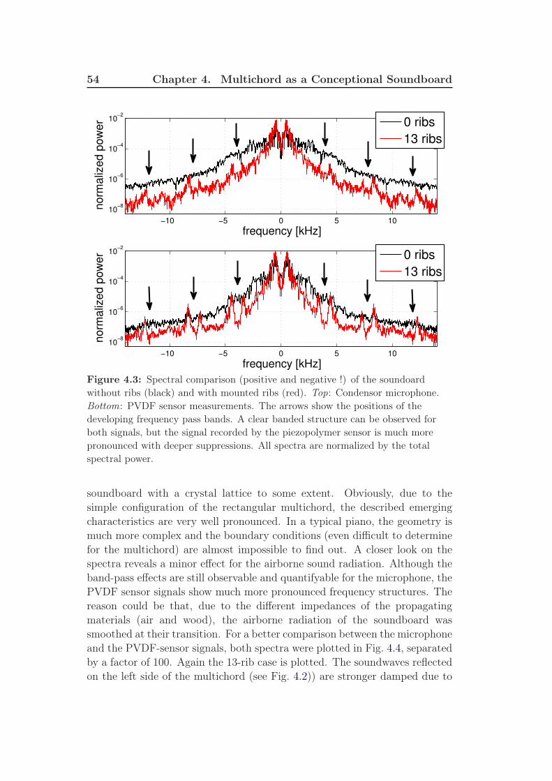
54 Chapter 4. Multichord as a Conceptional Soundboard
−10 −5 0 5 10
10−8
10−6
10−4
10−2
frequency [kHz]
norm
aliz
ed p
ow
er
0 ribs
13 ribs
−10 −5 0 5 10
10−8
10−6
10−4
10−2
frequency [kHz]
norm
aliz
ed p
ow
er
0 ribs
13 ribs
Figure 4.3: Spectral comparison (positive and negative !) of the soundoard
without ribs (black) and with mounted ribs (red). Top: Condensor microphone.
Bottom: PVDF sensor measurements. The arrows show the positions of the
developing frequency pass bands. A clear banded structure can be observed for
both signals, but the signal recorded by the piezopolymer sensor is much more
pronounced with deeper suppressions. All spectra are normalized by the total
spectral power.
soundboard with a crystal lattice to some extent. Obviously, due to thesimple configuration of the rectangular multichord, the described emergingcharacteristics are very well pronounced. In a typical piano, the geometry ismuch more complex and the boundary conditions (even difficult to determinefor the multichord) are almost impossible to find out. A closer look on thespectra reveals a minor effect for the airborne sound radiation. Although theband-pass effects are still observable and quantifyable for the microphone, thePVDF sensor signals show much more pronounced frequency structures. Thereason could be that, due to the different impedances of the propagatingmaterials (air and wood), the airborne radiation of the soundboard wassmoothed at their transition. For a better comparison between the microphoneand the PVDF-sensor signals, both spectra were plotted in Fig. 4.4, separatedby a factor of 100. Again the 13-rib case is plotted. The soundwaves reflectedon the left side of the multichord (see Fig. 4.2)) are stronger damped due to

4.3. Rib Scattering 55
0 2 4 6 8 10 12frequency [kHz]
norm
aliz
ed p
ow
er
condenser microphone
PVDF sensor
Figure 4.4: Direct comparison (only the positive frequency range) of the
piezopolymer (red) and microphone (black) measurements, with 13 mounted ribs.
The curves are normalized and seperated by a factor of 100 for a better
comparison.
the longer propagation length. This is clearly reflected by the less pronounced’left hand’ pass bands, nicely shown in Fig. 4.4, where both pass bands at ∼8kHz have different intensities.
Repeatability and Point of Attack of the Soundboard Excitation Inthe first part of the measurements, mounted strings were excited by controlledhammering (only gravity was the driving force). But then there was, of course,always a preference of the frequency modes matching the harmonics of thestrings. Since all relevant frequencies should be excited at once with the sameintensity, the strings were removed from the multichord, and a pulse excitation(also only driven by gravity) was performed. The most convenient results wereobtained by directly hitting the bridge. This also corresponds to the musicalexcitation, because the piano bridge is the ’soundboard entrance’ for thestring-generated soundwaves. Nevertheless, to check the occuring differencesby changing the excitation location, the point of attack was changed fromcentral on the bridge to decentral right within a void space between tworibs. There are observable differences, which are displayed in Fig. 4.5a. Nodeviations larger than 3% in peak position are found, instead one can expectlarge changes known from a piano string. While the bridge attack shows someadditional structure apart from the pass bands, the direct soundboard attackturns out to be smoother. The multichord bridge excitation was performedalways in the same manner, meaning that a specific mass was falling alwaysfrom the same height, developing a defined momentum. The reproducibility

56 Chapter 4. Multichord as a Conceptional Soundboard
0.45 0.46 0.47 0.48 0.49time [s]
am
plit
ude [a.u
.]
0 2 4 6 8frequency [kHz]
no
rma
lize
d p
ow
er
between−rib excitation
bridge excitation
(a) (b)
Figure 4.5: (a): The different excitation points with their spectral differences.
The bridge excitation (which is used throughout this investigation) as the red
curve, and the decentral excitation located in the middle of a void rib space as the
blue curve. The plots are also normalized and separated by a factor of 100 for a
better comparability. Beside that the pass-band structures of interest are basically
identical, the bridge excitation appears musically relevant, if the piano excitation
is considered.
(b): 15 independent excitations at the bridge of the multichord covering the same
time range. An almost perfect correlation (C = 0.995) between these curves secure
the reproducibility of the excitation.
of this excitation method is nicely shown in Fig. 4.5b, where 13 differentexcitations on the same location at the bridge are shown for the same timerange. An almost perfect correlation of C = 0.995 (see A.2.2) proves thatthe pulse excitation is almost perfectly reproducible, which is essential forthe measurements. Furthermore, the excitation amplitude was measured ina series of successive experiments, where the amplitude was found constantwith slight deviations. As we focus on the frequency analysis, the amplitudeof the hammering shall not be discussed here.
The next step in this investigation is to take a closer look at the positionsof the band edges and to analyze the underlying mode structure of thesoundboard. Examining a rib-free soundboard, two eigenmodes could befound: first the mode of the vibration along the string direction (which willbe then the ’ribbed’ part of the soundboard) and second the mode of thevibration along the length b4 (see Fig. 4.6 and Fig. 4.2) on the other side.Hence, the frequencies should be located at about ν1,n = c/(n · 2LSB) andν2,n = c/(n · 2LBR). Unfortunately, the frequencies are hard to identify,because the boundary conditions of the soundboard are not well defined(neither completely fixed, nor completely free). Since the material parameters

4.3. Rib Scattering 57
Figure 4.6: The
most important
longitudinal modes
of the investigated
multichord – LSB
and LBR.
are not known exactly either, the determination of the eigenmodes is left tothe measurements. To calculate the resonant frequencies, one needs the soundvelocity in the rib-free soundboard. With the help of two accelerometers,manufactured by Brüel & Kjær, which are commonly used, the sound velocitywithin the board was determined. There are two different kinds of velocities:the group velocity, which combines all frequencies within a wave, and the phasevelocity, which includes one single frequency. The excitation was performendby a single pulse, including all possible frequencies. Therefore, knowing thedistance between both accelerometers and the measured time delay of theexcitation, the group velocity can be determined. In the case of a ’rib-free’soundboard, the velocity was v0 ribs = 1145m/s. The ’ribbed’ soundboardexibits a value of v13 ribs = 773m/s. Hence, the sound velocity is reducedif ribs are mounted. The intuition is fully confirmed: Including scattererswill hinder the propagation of the sound wave, yielding a reduced soundvelocity. With the known lengths LSB = 0.99 m and LBR = 0.11 m (seeFig. 4.6), the resonant frequencies can be determined as ν1,1 = 578 Hz andν2,1 = 5205 Hz. In the measured spectrum of the ’rib-free’ soundboard themain characteristics appears between 250 Hz and 1050 Hz, which is, in verygood agreement with the resonant frequency ν1,1 = 578 Hz of the model. Theother resonant frequency ν2,1 = 5205 Hz from the model was not observed.
Given the assumptions above, 13 peaks within a pass band should befound. Actually only 10 peaks are well distinguishable (see Fig. 4.7) due tothe relatively simple modeling with LCM, where the ribs act as the masses andthe void spaces between the ribs act as the springs. The findings neverthelessare quite good and very convincing. It should be noted, that the frequenciesnear the pass-band edges are sensitive to any perturbations and can fall out ofthe band easily. This leads to a strong damping which makes them probablyhard to find in the frequency spectrum.
The second pass band is found in the frequency range from 4150 Hz to4865 Hz, the third from 8065 Hz to 8765 Hz and the forth from 11950 Hz to12665 Hz. The spectrum reveals no higher pass band, which means that theyare probably damped. Taking a closer look to the exact peak positions fromthe measurements and comparing these between the different bands, one finds,that these positions are exactly the same, only shifted by ν2 = 3900 Hz, which
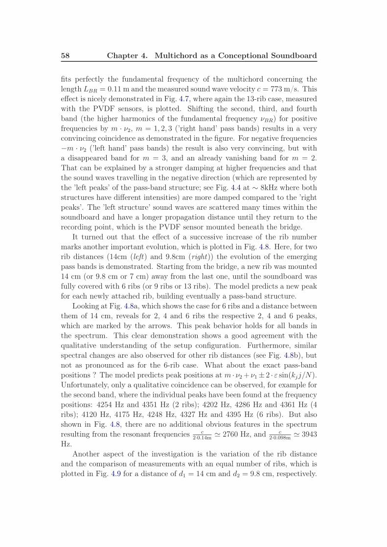
58 Chapter 4. Multichord as a Conceptional Soundboard
fits perfectly the fundamental frequency of the multichord concerning thelength LBR = 0.11 m and the measured sound wave velocity c = 773 m/s. Thiseffect is nicely demonstrated in Fig. 4.7, where again the 13-rib case, measuredwith the PVDF sensors, is plotted. Shifting the second, third, and fourthband (the higher harmonics of the fundamental frequency νBR) for positivefrequencies by m · ν2, m = 1, 2, 3 (’right hand’ pass bands) results in a veryconvincing coincidence as demonstrated in the figure. For negative frequencies−m · ν2 (’left hand’ pass bands) the result is also very convincing, but witha disappeared band for m = 3, and an already vanishing band for m = 2.That can be explained by a stronger damping at higher frequencies and thatthe sound waves travelling in the negative direction (which are represented bythe ’left peaks’ of the pass-band structure; see Fig. 4.4 at ∼ 8kHz where bothstructures have different intensities) are more damped compared to the ’rightpeaks’. The ’left structure’ sound waves are scattered many times within thesoundboard and have a longer propagation distance until they return to therecording point, which is the PVDF sensor mounted beneath the bridge.
It turned out that the effect of a successive increase of the rib numbermarks another important evolution, which is plotted in Fig. 4.8. Here, for tworib distances (14cm (left) and 9.8cm (right)) the evolution of the emergingpass bands is demonstrated. Starting from the bridge, a new rib was mounted14 cm (or 9.8 cm or 7 cm) away from the last one, until the soundboard wasfully covered with 6 ribs (or 9 ribs or 13 ribs). The model predicts a new peakfor each newly attached rib, building eventually a pass-band structure.
Looking at Fig. 4.8a, which shows the case for 6 ribs and a distance betweenthem of 14 cm, reveals for 2, 4 and 6 ribs the respective 2, 4 and 6 peaks,which are marked by the arrows. This peak behavior holds for all bands inthe spectrum. This clear demonstration shows a good agreement with thequalitative understanding of the setup configuration. Furthermore, similarspectral changes are also observed for other rib distances (see Fig. 4.8b), butnot as pronounced as for the 6-rib case. What about the exact pass-bandpositions ? The model predicts peak positions at m · ν2+ ν1± 2 · ε sin(kjj/N).Unfortunately, only a qualitative coincidence can be observed, for example forthe second band, where the individual peaks have been found at the frequencypositions: 4254 Hz and 4351 Hz (2 ribs); 4202 Hz, 4286 Hz and 4361 Hz (4ribs); 4120 Hz, 4175 Hz, 4248 Hz, 4327 Hz and 4395 Hz (6 ribs). But alsoshown in Fig. 4.8, there are no additional obvious features in the spectrumresulting from the resonant frequencies c
2·0.14m≃ 2760 Hz, and c
2·0.098m≃ 3943
Hz.Another aspect of the investigation is the variation of the rib distance
and the comparison of measurements with an equal number of ribs, which isplotted in Fig. 4.9 for a distance of d1 = 14 cm and d2 = 9.8 cm, respectively.

4.3. Rib Scattering 59
−1000 −800 −600 −400 −200 0 200 400 600 800 1000
frequency [Hz]
inte
nsity [dB
]
−1000 −800 −600 −400 −200 0 200 400 600 800 1000
frequency [Hz]
inte
nsity [dB
]
0 Hz
3.9 kHz
7.8 kHz
11.7 kHz
Figure 4.7: Structure comparison of the shifted pass bands measured at the
multichord. Top: PVDF sensor beneath the bridge, and bottom: microphone
measurement.
The first band structure (−1000 Hz to 1000 Hz) is shown as the black line; the
second structure shifted by 3900 Hz depicted as red curve right below; the third
band shifted by 7800 Hz (blue) and the forth band with a shift of 11700 Hz
(green). Independent of the number of the mounted ribs and the distance between
them, the shift is always m · 3900 Hz, m = 1, 2, 3. The coincidence of the
individual peaks (e.g., at ±280Hz, ±400Hz, ±460Hz, ±540Hz etc.) within the
specific bands is highly significant. The red, blue and green curves are enhanced
by a factor of 100 for a better comparability.
Looking at the peak positions, actually only little changes can be observed.The basic structure of the pass bands remains constant.
Finally, the lifetime of the pass-band modes is also discussed. Therefore,a time-dependent frequency analysis with short time slices of 5 ms has beenperformed. It can be concluded from Fig. 4.10, that the above-mentioned’pass bands’ have significantly longer decay time within the instrument.Considering the airborne sound measurements, this effect can also be observed,without being that clear. To investigate this lifetime behavior in particular,the decay factor γ is determined for all frequencies in the next chapter.
In conclusion, frequency ’pass bands’ with a bandwith of 2ε were found
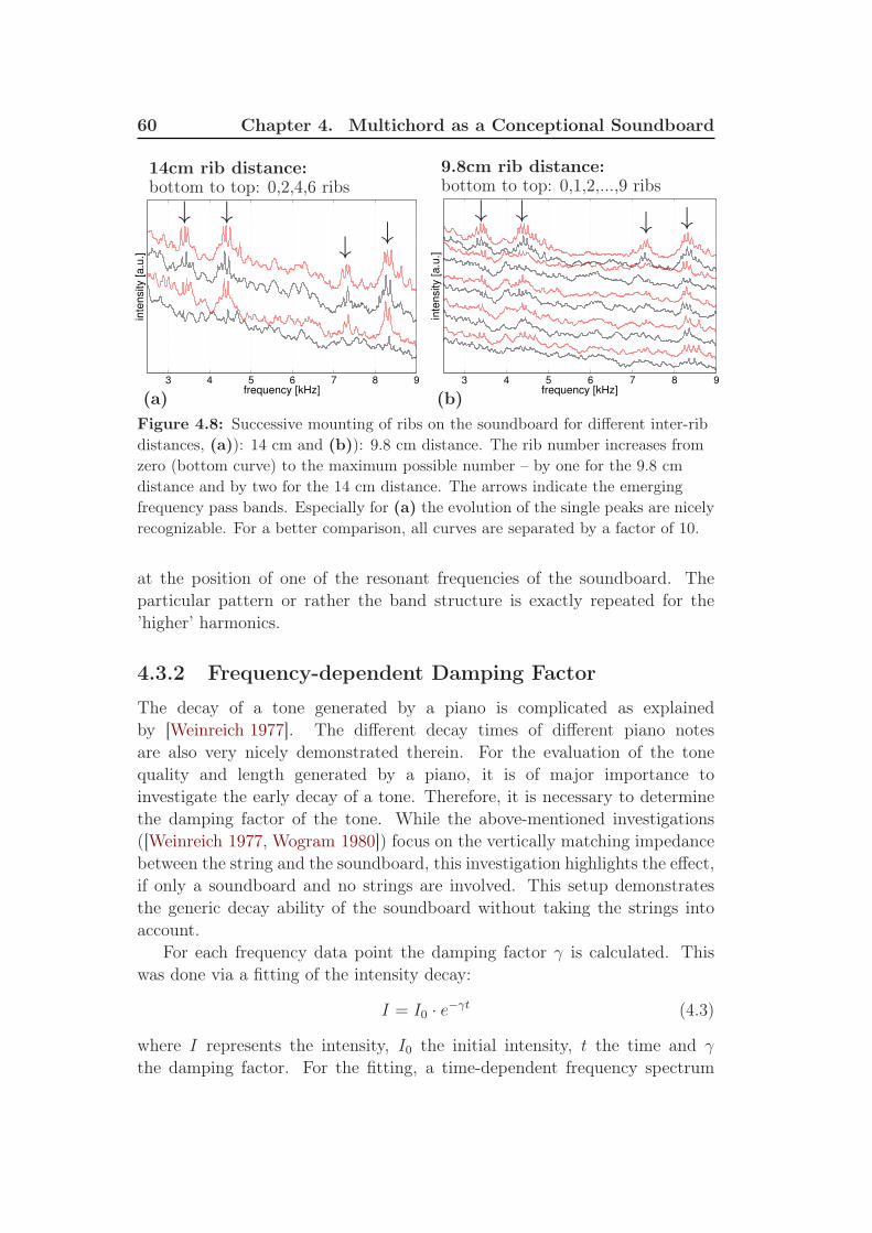
60 Chapter 4. Multichord as a Conceptional Soundboard
3 4 5 6 7 8 9frequency [kHz]
inte
nsity [a.u
.]
3 4 5 6 7 8 9frequency [kHz]
inte
nsity [a.u
.]
14cm rib distance: 9.8cm rib distance:bottom to top: 0,2,4,6 ribs bottom to top: 0,1,2,...,9 ribs
(a) (b)
↓ ↓↓ ↓
↓ ↓ ↓ ↓
Figure 4.8: Successive mounting of ribs on the soundboard for different inter-rib
distances, (a)): 14 cm and (b)): 9.8 cm distance. The rib number increases from
zero (bottom curve) to the maximum possible number – by one for the 9.8 cm
distance and by two for the 14 cm distance. The arrows indicate the emerging
frequency pass bands. Especially for (a) the evolution of the single peaks are nicely
recognizable. For a better comparison, all curves are separated by a factor of 10.
at the position of one of the resonant frequencies of the soundboard. Theparticular pattern or rather the band structure is exactly repeated for the’higher’ harmonics.
4.3.2 Frequency-dependent Damping Factor
The decay of a tone generated by a piano is complicated as explainedby [Weinreich 1977]. The different decay times of different piano notesare also very nicely demonstrated therein. For the evaluation of the tonequality and length generated by a piano, it is of major importance toinvestigate the early decay of a tone. Therefore, it is necessary to determinethe damping factor of the tone. While the above-mentioned investigations([Weinreich 1977, Wogram 1980]) focus on the vertically matching impedancebetween the string and the soundboard, this investigation highlights the effect,if only a soundboard and no strings are involved. This setup demonstratesthe generic decay ability of the soundboard without taking the strings intoaccount.
For each frequency data point the damping factor γ is calculated. Thiswas done via a fitting of the intensity decay:
I = I0 · e−γt (4.3)
where I represents the intensity, I0 the initial intensity, t the time and γ
the damping factor. For the fitting, a time-dependent frequency spectrum

4.3. Rib Scattering 61
8 8.5
no
rma
lize
d p
ow
er
8 8.5frequency [kHz]
8 8.5
10cm rib distance
14cm rib distance
2 ribs 4 ribs 6 ribs
Figure 4.9: PVDF
spectral comparison for
equal rib number (left
– 2 ribs; middle – 4
ribs; right – 6 ribs)
with different rib
distances (red – 14cm;
black – 9.8cm). The
third pass band (8 kHz
to 8.9 kHz) is shown.
Curves are normalized
to spectral power.
Figure 4.10:
Time-dependent
frequency
spectrum of the
resonance board
with 0 ribs (top)
and with 13 ribs
(bottom). The
soundboard is
excited once and
the decay of the
signal is observed
by the
piezopolymer
(left) and the
microphone
(right).

62 Chapter 4. Multichord as a Conceptional Soundboard
Figure 4.11:
Demonstrating the
algorithm for the
determination of the
damping factor at a certain
frequency. The plotted
curves are separated by a
factor of 10 for a better
comparability. Shown is
the case for 6150 Hz. The
decay with ribs and
without ribs is fitted with
Eq. 4.3. Comparing the fits
yields the difference in the
damping factor.0 0.05 0.1 0.15 0.2
time [s]
inte
nsity [a.u
.]
intensity decay at 6150 Hz (with ribs)
fitting (with ribs)
intensity decay at 6150 Hz (without ribs)
fitting (without ribs)
was calculated (e.g. Fig. 4.10). An exemplary calculation is performed inFig. 4.11 at 6150 Hz, including the difference for the damping factor withribs and without. The determined values for γ were γnone = 156.21/s andγribs = 92.71/s, meaning a faster intensity decay without ribs, compared tothe ’ribbed’ case.
This analysis is extended consequently to the audible frequency spectrumas depicted in Fig. 4.12. As can be seen from the graph, the damping factorand the respective decay factor vary drastically with frequency. Consistently,a drop in the damping factor between 3 kHz and about 10 kHz can be seen– the soundboard radiates longer in this range if the ribs are attached. Thiseffect becomes more pronounced, when a larger number of ribs are mountedto the soundboard.
4.3.3 Comparison: Scattering Model vs. Experimental
Data
Using the adjusted LCM model explained in chapter 2 and the section above,the theoretical peaks of the pass bands will be fitted to the measured peakpositions. Therefore, the ribs represent the masses in the model, while thespaces between the ribs represent the springs.
The acoustic dispersion relation (see Eq. 2.7) is given by
ωk = 2 · ω0 ·∣
∣
∣
∣
sin
(
π
2· nN
)∣
∣
∣
∣
(4.4)
ωk represents the frequency of mode k = (2πn)/(aN) with a as the ribdistance, ω0 is the fundamental vibrating frequency of the soundboard. n
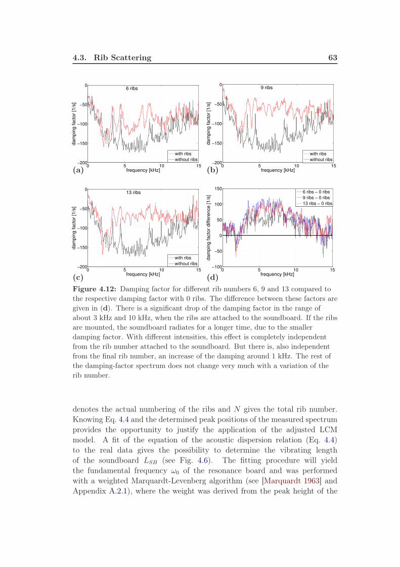
4.3. Rib Scattering 63
0 5 10 15−200
−150
−100
−50
0
frequency [kHz]
dam
pin
g facto
r [1
/s]
6 ribs
with ribs
without ribs
0 5 10 15−200
−150
−100
−50
0
frequency [kHz]
dam
pin
g facto
r [1
/s]
9 ribs
with ribs
without ribs
0 5 10 15−200
−150
−100
−50
0
frequency [kHz]
dam
pin
g facto
r [1
/s]
13 ribs
with ribs
without ribs
0 5 10 15−100
−50
0
50
100
150
frequency [kHz]
dam
pin
g facto
r diffe
rence [1/s
]
6 ribs − 0 ribs
9 ribs − 0 ribs
13 ribs − 0 ribs
(a) (b)
(c) (d)
Figure 4.12: Damping factor for different rib numbers 6, 9 and 13 compared to
the respective damping factor with 0 ribs. The difference between these factors are
given in (d). There is a significant drop of the damping factor in the range of
about 3 kHz and 10 kHz, when the ribs are attached to the soundboard. If the ribs
are mounted, the soundboard radiates for a longer time, due to the smaller
damping factor. With different intensities, this effect is completely independent
from the rib number attached to the soundboard. But there is, also independent
from the final rib number, an increase of the damping around 1 kHz. The rest of
the damping-factor spectrum does not change very much with a variation of the
rib number.
denotes the actual numbering of the ribs and N gives the total rib number.Knowing Eq. 4.4 and the determined peak positions of the measured spectrumprovides the opportunity to justify the application of the adjusted LCMmodel. A fit of the equation of the acoustic dispersion relation (Eq. 4.4)to the real data gives the possibility to determine the vibrating lengthof the soundboard LSB (see Fig. 4.6). The fitting procedure will yieldthe fundamental frequency ω0 of the resonance board and was performedwith a weighted Marquardt-Levenberg algorithm (see [Marquardt 1963] andAppendix A.2.1), where the weight was derived from the peak height of the
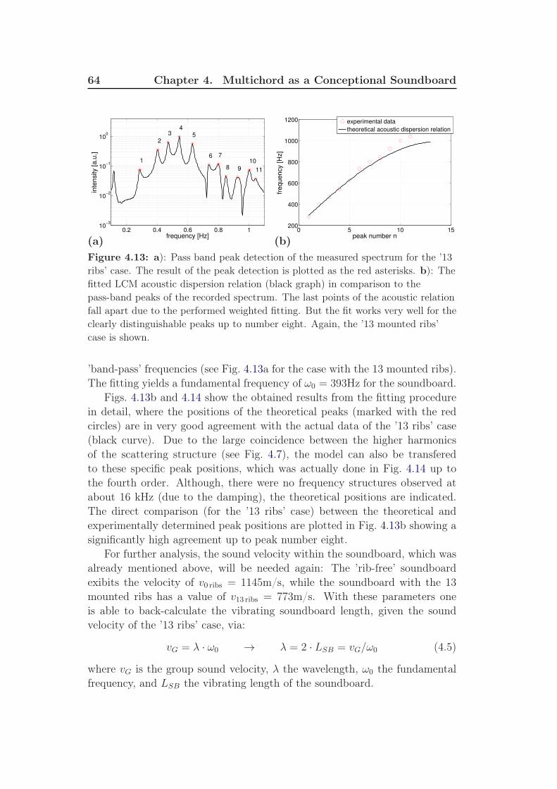
64 Chapter 4. Multichord as a Conceptional Soundboard
0.2 0.4 0.6 0.8 110
−3
10−2
10−1
100
1
2
34
5
6 7
8 9
10
11
frequency [Hz]
inte
nsity [
a.u
.]
0 5 10 15200
400
600
800
1000
1200
fre
qu
en
cy [
Hz]
peak number n
experimental data
theoretical acoustic dispersion relation
(a) (b)
Figure 4.13: a): Pass band peak detection of the measured spectrum for the ’13
ribs’ case. The result of the peak detection is plotted as the red asterisks. b): The
fitted LCM acoustic dispersion relation (black graph) in comparison to the
pass-band peaks of the recorded spectrum. The last points of the acoustic relation
fall apart due to the performed weighted fitting. But the fit works very well for the
clearly distinguishable peaks up to number eight. Again, the ’13 mounted ribs’
case is shown.
’band-pass’ frequencies (see Fig. 4.13a for the case with the 13 mounted ribs).The fitting yields a fundamental frequency of ω0 = 393Hz for the soundboard.
Figs. 4.13b and 4.14 show the obtained results from the fitting procedurein detail, where the positions of the theoretical peaks (marked with the redcircles) are in very good agreement with the actual data of the ’13 ribs’ case(black curve). Due to the large coincidence between the higher harmonicsof the scattering structure (see Fig. 4.7), the model can also be transferedto these specific peak positions, which was actually done in Fig. 4.14 up tothe fourth order. Although, there were no frequency structures observed atabout 16 kHz (due to the damping), the theoretical positions are indicated.The direct comparison (for the ’13 ribs’ case) between the theoretical andexperimentally determined peak positions are plotted in Fig. 4.13b showing asignificantly high agreement up to peak number eight.
For further analysis, the sound velocity within the soundboard, which wasalready mentioned above, will be needed again: The ’rib-free’ soundboardexibits the velocity of v0 ribs = 1145m/s, while the soundboard with the 13mounted ribs has a value of v13 ribs = 773m/s. With these parameters oneis able to back-calculate the vibrating soundboard length, given the soundvelocity of the ’13 ribs’ case, via:
vG = λ · ω0 → λ = 2 · LSB = vG/ω0 (4.5)
where vG is the group sound velocity, λ the wavelength, ω0 the fundamentalfrequency, and LSB the vibrating length of the soundboard.

4.3. Rib Scattering 65
−1000 −500 0 500 1000frequency [Hz]
inte
nsity [a.u
.]
0 2 4 6 8 10 12 14 16 18frequency [Hz]
inte
nsity [a.u
.]
theoretical peaks
experimental data
peak detection
Figure 4.14: The fitted theoretical peaks (red cicles) from the passband (LCM
model) in comparison with the peaks of the experimental data shown for different
frequency ranges. Top: A close-up for the identification of the individual peaks
(-1.2 kHz to 1.2 kHz). Bottom: The broad range to show the position of the other
pass bands in comparison with the theoretical peak locations (1.2 kHz to 18 kHz).
Knowing Eq. 4.5, the sound velocity v13 ribs = 773m/s and the fundamentalfrequency ω0 = 393Hz will provide the length of the vibrating soundboard viaback-calculation, which is Lvibr = 0.98m. This is in very good agreement withthe ’rib-mounted’ vibrating length of the resonance board with LSB = 0.99m(Whole multichord length (1.2m) minus boundaries (2x0.05m) minus distancebetween boundary bridge and excitation bridge (LBR = 0.11m; see Fig. 4.2)),justifying the use of the adjusted LCM not only for the understanding of thescattering effects of the sound-wave propagation in patterned materials, butalso for the exact position of the emerging peaks in the spectrum.
Also a qualitative discrimination of the acoustic dispersion relationbetween the different rib distances could be drawn, which is plotted inFig. 4.15. The specific relations for rib distances 7cm (blue), 9.8cm (red),and 14cm (green) are compared, while the inset of the same figure shows thetheoretical trend for the mounted 13 ribs. A successively better agreementbetween theory and measurement can be observed with an increasing ribnumber. This result also fully confirms the intuition, because many obstaclesare closer to the LCM model, which was actually proposed for the acoustic

66 Chapter 4. Multichord as a Conceptional Soundboard
2 4 6 80
200
400
600
800
1000
1200p
ositio
n in
Hz
# peaks
6 ribs
9 ribs
13 ribs
po
sitio
n in
Hz
# peaks
theo. dispersion (13 ribs)
Figure 4.15: Large plot : The different measured dispersion relations for the
various rib distances: ’6 ribs’ – green, ’9 ribs’ – red, ’13 ribs’ – blue. Inset : The
theoretical dispersion relation for the ’13 ribs’ case
dispersion relation on an atomic level.Possible alternatives to the LCM, such as FEM (finite-element method)
simulations, were not employed due to the time-consuming procedure. TheLCM is a simple approach indeed, but due to the very good agreement ofthe peak positions between this model and the measured data with variationssmaller than 3%, it is sufficient to make predictions about the positions of theemerging peaks.
4.4 Chapter Conclusion
In this chapter, the dramatic effect obstacles mounted on a multichordsoundboard may have on the propagation of sound waves is demonstrated.To some extent, the results hold for any vibrating body with a regularlystructured surface which radiates sound when excited. From generalarguments, it follows that the spectrum of the multichord and the piano hasmany similarities as can be seen later in the ’Bechstein piano’ chapter 5.Nevertheless, the piano soundboard geometry used is different and the modalstructure is not as clear as on the rectangular multichord soundboard.
A specifically designed setup with minimal parameter variations was used

4.4. Chapter Conclusion 67
to have full control of the reproducibility of the results3. The number ofribs mounted and the spacing between the ribs were varied, and as a result,a heavy influence of even few ribs on the sound radiation and propagationhas been found. The position of the passing frequencies found are theeigenmodes of the structured soundboard, which correspond with qualitativeband theory (see Sec. 4.1), analogous to the theory of phonons in solidstate physics – the so called LCM model. These certain eigenfrequencies aredetermined experimentally and verified theoretically. Knowing the positions ofthe pass-band peaks, the ’length’ of the chain (which is the ’ribbed’ vibratinglength of the multichord) could be back-calculated.
The question arises how to circumvent the unwanted suppression orincrease of certain frequencies, if ribs must be mounted to strengthen thesoundboard mechanically. As explained in the next chapter for the piano, astructured band can be easily eliminated, if disorder is introduced into thesystem.
3The exception was the sucessive mounting of the ribs.

Chapter 5
The Real Piano: Bechstein
’Zimmermann Z.3/116’
One of the main aims of this investigation was the application of the PVDFsensors in a genuine instrument. A cooperation with the piano manufacturer’C. Bechstein Pianofortefabrik’ [Bechstein 2005] provided the opportunity tomount these sensors in one of their pianos.The structure of this chapter is as follows: First, the design and constructionof an upright piano is explained (Sec. 5.1). Then, every step of the assemblyof the piano is described. The PVDF sensors are mounted within the Pianostructure from the beginning of the assembly process.
5.1 Piano Assembly
The upright piano ’Zimmermann Z.3/116 ’ (see Fig. 5.1), which is thesmallest model in the Zimmermann series, manufactured by ’C. BechsteinPianofortefabrik’, was the investigated object. The assembly of a piano1
comprises several individual construction steps (see Tab. 5.1 and theadditional pictures in Fig. 5.3b&c and Fig. 5.4 for each stage), using acombination of automated machinery and hand crafting. Following the listingin Tab. 5.1, the bridges (treble and bass bridge) on one side and 11 ribs onthe other side are glued to the empty soundboard, which has a dimension ofwidth x height x depth: 146cm x 93cm x 0.8cm (step no. 1a & 1b). Aftera drying time of about two hours, the back of the board was varnished (stepno. 2). To provide stability and the basis for further mountings, the wholesoundboard was attached at a wooden frame (step no. 3). With the finalvarnishing on the front side (step no. 4), the moisture level within the boardis fixed. The next step in the course of the construction process comprises theattachment of the metal frame, which includes the mounted strings already(step no. 5). The last two steps2 in the piano assembly are the installation
1The description of the construction relies solely on personal experience of the
investigator. A detailed reference of the typical assembly workflow has not been found.
This expert knowledge was acquired during several visits of the Bechstein manufacturing
center.2Beside the individual tuning of the strings.
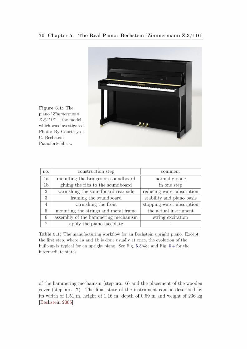
70 Chapter 5. The Real Piano: Bechstein ’Zimmermann Z.3/116’
Figure 5.1: The
piano ’Zimmermann
Z.3/116 ’ – the model
which was investigated.
Photo: By Courtesy of
C. Bechstein
Pianofortefabrik.
no. construction step comment
1a mounting the bridges on soundboard normally done1b gluing the ribs to the soundboard in one step2 varnishing the soundboard rear side reducing water absorption3 framing the soundboard stability and piano basis4 varnishing the front stopping water absorption5 mounting the strings and metal frame the actual instrument6 assembly of the hammering mechanism string excitation7 apply the piano faceplate -
Table 5.1: The manufacturing workflow for an Bechstein upright piano. Except
the first step, where 1a and 1b is done usually at once, the evolution of the
built-up is typical for an upright piano. See Fig. 5.3b&c and Fig. 5.4 for the
intermediate states.
of the hammering mechanism (step no. 6) and the placement of the woodencover (step no. 7). The final state of the instrument can be described byits width of 1.51 m, height of 1.16 m, depth of 0.59 m and weight of 236 kg[Bechstein 2005].
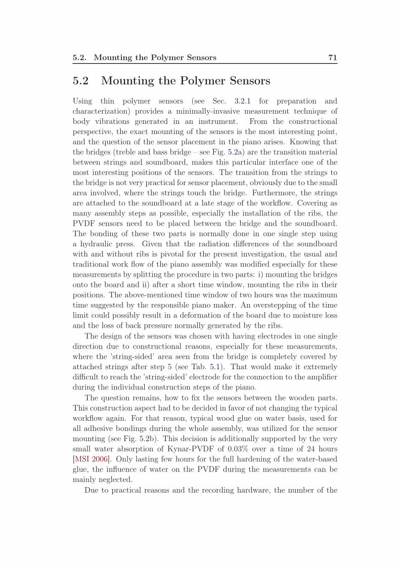
5.2. Mounting the Polymer Sensors 71
5.2 Mounting the Polymer Sensors
Using thin polymer sensors (see Sec. 3.2.1 for preparation andcharacterization) provides a minimally-invasive measurement technique ofbody vibrations generated in an instrument. From the constructionalperspective, the exact mounting of the sensors is the most interesting point,and the question of the sensor placement in the piano arises. Knowing thatthe bridges (treble and bass bridge – see Fig. 5.2a) are the transition materialbetween strings and soundboard, makes this particular interface one of themost interesting positions of the sensors. The transition from the strings tothe bridge is not very practical for sensor placement, obviously due to the smallarea involved, where the strings touch the bridge. Furthermore, the stringsare attached to the soundboard at a late stage of the workflow. Covering asmany assembly steps as possible, especially the installation of the ribs, thePVDF sensors need to be placed between the bridge and the soundboard.The bonding of these two parts is normally done in one single step usinga hydraulic press. Given that the radiation differences of the soundboardwith and without ribs is pivotal for the present investigation, the usual andtraditional work flow of the piano assembly was modified especially for thesemeasurements by splitting the procedure in two parts: i) mounting the bridgesonto the board and ii) after a short time window, mounting the ribs in theirpositions. The above-mentioned time window of two hours was the maximumtime suggested by the responsible piano maker. An overstepping of the timelimit could possibly result in a deformation of the board due to moisture lossand the loss of back pressure normally generated by the ribs.
The design of the sensors was chosen with having electrodes in one singledirection due to constructional reasons, especially for these measurements,where the ’string-sided’ area seen from the bridge is completely covered byattached strings after step 5 (see Tab. 5.1). That would make it extremelydifficult to reach the ’string-sided’ electrode for the connection to the amplifierduring the individual construction steps of the piano.
The question remains, how to fix the sensors between the wooden parts.This construction aspect had to be decided in favor of not changing the typicalworkflow again. For that reason, typical wood glue on water basis, used forall adhesive bondings during the whole assembly, was utilized for the sensormounting (see Fig. 5.2b). This decision is additionally supported by the verysmall water absorption of Kynar-PVDF of 0.03% over a time of 24 hours[MSI 2006]. Only lasting few hours for the full hardening of the water-basedglue, the influence of water on the PVDF during the measurements can bemainly neglected.
Due to practical reasons and the recording hardware, the number of the

72 Chapter 5. The Real Piano: Bechstein ’Zimmermann Z.3/116’
(a)
(b)
(c)
Figure 5.2: (a): The stand-alone bridges of the upright piano (left : treble bridge;
right : bass bridge). (b): The bridge covered with wood glue. The PVDF sensors
are already in place, right before the brigde is glued onto the soundboard. (c):
Finally after the mounting: The sensor electrodes (red ellipse) can be seen very
nicely.
body vibration sensors is limited to six. The selected locations (see Fig. 5.3aas the filled red squares) were chosen for several reasons; on the one handto cover as well as possible the whole length of the treble piano bridge andtherefore a wide range of the tone pitch, and on the other hand, to be able torecord differences that possibly occur, if a sensor is placed right under a ribor not (see Fig. 5.3, especially the locations of PVDF1 / PVDF2 and PVDF4/ PVDF5). After the polymer sensors are fully installed, only two small partsof the sputtered electrodes (top and bottom) are sticking out as the ’onlyevidence’ of the sensors’ presence. The possible PVDF perturbation of thesound propagation within the piano can also be mainly neglected by reason ofthe matching impedances of wood and PVDF [MSI 2006, Bucur 2006]. Givena width of 3cm for the treble bridge, the piezoelectric sensors (see Fig. 3.7b)are placed symmetrically with regard to the sputtered rectangular area, i.e.the middle of the squared electrode surface is located right under the middle
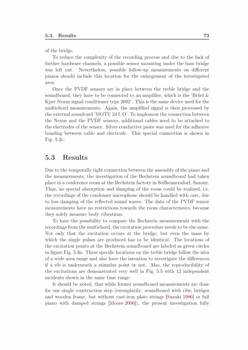
5.3. Results 73
of the bridge.To reduce the complexity of the recording process and due to the lack of
further hardware channels, a possible sensor mounting under the bass bridgewas left out. Nevertheless, possible follow-up measurements on differentpianos should include this location for the enlargement of the investigatedarea.
Once the PVDF sensors are in place between the treble bridge and thesoundboard, they have to be connected to an amplifier, which is the ’Brüel &Kjær Nexus signal conditioner type 2692’. This is the same device used for themultichord measurements. Again, the amplified signal is then processed bythe external soundcard ’MOTU 24 I/O’. To implement the connection betweenthe Nexus and the PVDF sensors, additional cables need to be attached tothe electrodes of the sensor. Silver conductive paste was used for the adhesivebonding between cable and electrode. This special connection is shown inFig. 5.2c.
5.3 Results
Due to the temporally tight connection between the assembly of the piano andthe measurements, the investigation of the Bechstein soundboard had takenplace in a conference room at the Bechstein factory in Seifhennersdorf, Saxony.Thus, no special absorption and damping of the room could be realized, i.e.the recordings of the condenser microphone should be handled with care, dueto less damping of the reflected sound waves. The data of the PVDF sensormeasurements have no restrictions towards the room characteristics, becausethey solely measure body vibrations.
To have the possibility to compare the Bechstein measurements with therecordings from the multichord, the excitation procedure needs to be the same.Not only that the excitation occurs at the bridge, but even the mass bywhich the single pulses are produced has to be identical. The locations ofthe excitation points at the Bechstein soundboard are labeled as green circlesin figure Fig. 5.3a. These specific locations on the treble bridge follow the ideaof a wide area range and also have the intention to investigate the differencesif a rib is underneath a stimulus point or not. Also, the reproducibility ofthe excitations are demonstrated very well in Fig. 5.5 with 12 independentincidents shown in the same time range.
It should be noted, that while former soundboard measurements are donefor one single construction step (exemplarily: soundboard with ribs, bridgesand wooden frame, but without cast-iron plate strings [Suzuki 1986] or fullpiano with damped strings [Moore 2006]), the present investigation fully

74 Chapter 5. The Real Piano: Bechstein ’Zimmermann Z.3/116’
(a)
(b) (c)
Figure 5.3: (a):Design drawing of the Bechstein ’Z.3/116’ soundboard, including
all parts on the front and back; units given in [mm]. Also depicted in the graph
are the excitation points at the bridge (six green cicles) and the positions of the
PVDF sensors (six red squares). The numbers 1 and 11 clarify the rib numbering.
(b): Front side of the soundboard with the PVDF sensors already mounted in
their respective positions. (c): The same for the rear side of the soundboard
including the bonded ribs.
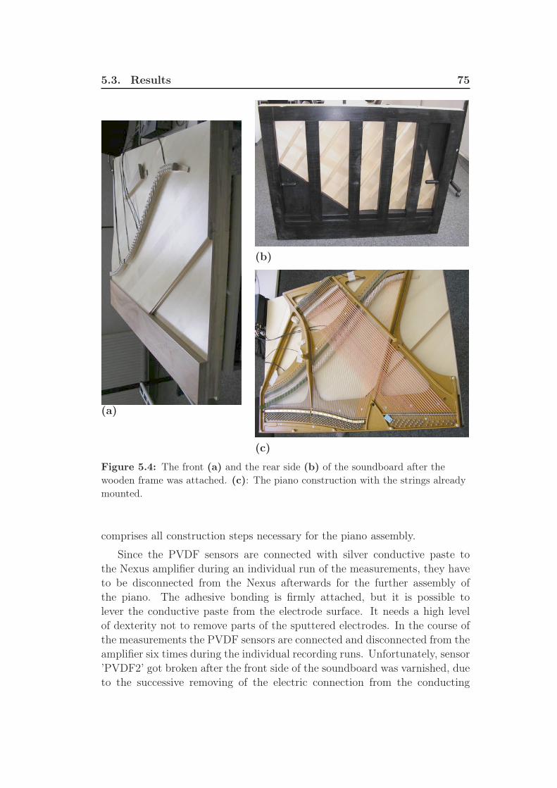
5.3. Results 75
(a)
(b)
(c)
Figure 5.4: The front (a) and the rear side (b) of the soundboard after the
wooden frame was attached. (c): The piano construction with the strings already
mounted.
comprises all construction steps necessary for the piano assembly.
Since the PVDF sensors are connected with silver conductive paste tothe Nexus amplifier during an individual run of the measurements, they haveto be disconnected from the Nexus afterwards for the further assembly ofthe piano. The adhesive bonding is firmly attached, but it is possible tolever the conductive paste from the electrode surface. It needs a high levelof dexterity not to remove parts of the sputtered electrodes. In the course ofthe measurements the PVDF sensors are connected and disconnected from theamplifier six times during the individual recording runs. Unfortunately, sensor’PVDF2’ got broken after the front side of the soundboard was varnished, dueto the successive removing of the electric connection from the conducting

76 Chapter 5. The Real Piano: Bechstein ’Zimmermann Z.3/116’
Figure 5.5: 12
different excitations
for the same time
range (0.006 s to
0.027 s),
demonstrating the
repeatability of the
excitation
mechanism.0.01 0.015 0.02 0.025
time [s]
am
plit
ude [a.u
.]
Figure 5.6: One individual
excitation recorded by two
different PVDF sensors –
’PVDF2’ and ’PVDF3’. The
location of the excitation in
this case was ’EX 2’ (see
Fig. 5.3a), which is situated
exactly above ’PVDF2’. This
demonstrates that the
maximum amplitude is not
neccessarily related to the
initial amplitude. Details in
the text.7.2 7.3 7.4 7.5 7.6
−0.2
−0.1
0
0.1
0.2
0.3
0.4
time in [s]
dyn. fo
rce in [N
]
sensor PVDF2sensor PVDF3
layer. Since the metal frame with the strings are in place (step 5 in Tab. 5.1),it is more practical in the further assembly process to keep the connection tothe PVDF sensors permanently. This will also prevent further damage of theelectrodes.
5.3.1 Pulse Amplitude
An important and interesting aspect of the measurements is the evolutionof the dynamic force amplitude at the bridge-soundboard transition and thequestion of its rib dependency. Therefore, the maximum amplitude for eachexcitation and for each PVDF sensor was determined. Measurements showthat the initial amplitude is not mandatorily the overall maximum amplitude.As one takes a look at Fig. 5.6, this behavior is exactly demonstrated.
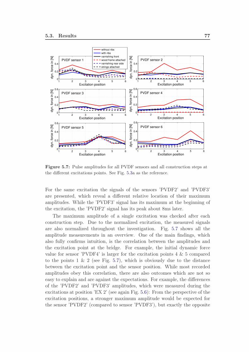
5.3. Results 77
1 2 3 4 5 60
0.2
0.4
PVDF sensor 1
Excitation position
dyn
. fo
rce
in
[N
]
without ribs
with ribs
varnishing front
wood frame attached
varnishing rear side
strings attached
1 2 3 4 5 60
0.2
0.4
PVDF sensor 2
Excitation position
dyn
. fo
rce
in
[N
]
1 2 3 4 5 60
0.2
0.4
0.6
PVDF sensor 3
Excitation position
dyn
. fo
rce
in
[N
]
1 2 3 4 5 60
0.2
0.4
0.6
PVDF sensor 4
Excitation position
dyn
. fo
rce
in
[N
]
1 2 3 4 5 60
0.2
0.4
0.6
PVDF sensor 5
Excitation position
dyn
. fo
rce
in
[N
]
1 2 3 4 5 60
0.2
0.4
0.6
PVDF sensor 6
Excitation position
dyn
. fo
rce
in
[N
]
Figure 5.7: Pulse amplitudes for all PVDF sensors and all construction steps at
the different excitations points. See Fig. 5.3a as the reference.
For the same excitation the signals of the sensors ’PVDF2’ and ’PVDF3’are presented, which reveal a different relative location of their maximumamplitudes. While the ’PVDF3’ signal has its maximum at the beginning ofthe excitation, the ’PVDF2’ signal has its peak about 8ms later.
The maximum amplitude of a single excitation was checked after eachconstruction step. Due to the normalized excitation, the measured signalsare also normalized throughout the investigation. Fig. 5.7 shows all theamplitude measurements in an overview. One of the main findings, whichalso fully confirms intuition, is the correlation between the amplitudes andthe excitation point at the bridge. For example, the initial dynamic forcevalue for sensor ’PVDF4’ is larger for the excitation points 4 & 5 comparedto the points 1 & 2 (see Fig. 5.7), which is obviously due to the distancebetween the excitation point and the sensor position. While most recordedamplitudes obey this correlation, there are also outcomes which are not soeasy to explain and are against the expectations. For example, the differencesof the ’PVDF2’ and ’PVDF3’ amplitudes, which were measured during theexcitations at position ’EX 2’ (see again Fig. 5.6): From the perspective of theexcitation positions, a stronger maximum amplitude would be expected forthe sensor ’PVDF2’ (compared to sensor ’PVDF3’), but exactly the opposite

78 Chapter 5. The Real Piano: Bechstein ’Zimmermann Z.3/116’
has been found. In that case depicted in Fig. 5.6 the ’PVDF3’ maximumamplitude is 1.5 times stronger then the ’PVDF2’ signal. One explanationfor this effect could be the positive interference of scattered waves within thesoundboard, but more likely is another explanation: A large value recorded bythe PVDF sensors means a large acceleration between the soundboard and thebridge, not neccessarily a large net force. Therefore, two signals with the sameenergy content are able to generate amplitudes, which can be quite different.The present case with an excitation at position ’EX 2’ shows the maximumamplitude at the position of ’PVDF3’. A good picture for an explanation ofthis effect is a stroke of the whip, where the outer end of the whip is much moreaccelerated compared to the starting point. But nevertheless, it is noticeablethat the overall signal envelope (see Fig. 5.6) for both signals (except for somesingle peak values) have the same appearence.
Furthermore, except for sensor ’PVDF5’, it was found that there is alarge difference regarding the amplitudes between steps 1a and 1b (referenceTab. 5.1). The mounting of additional ribs onto the soundboard results in asignificant damping of the amplitude. For example, the largest difference wasfound for the sensor ’PVDF2’ at excitation position ’EX 3’, where a factorof 2.7 (0.40 N (rib-free) to 0.15 N (ribbed)) was determined (see Fig. 5.7).The average of the force amplitude for all sensors changed from 0.23 N(without ribs) to 0.14 N (with ribs). This amplitude drop at the measurementpoints can be explained by scattering of the acoustic sound wave at the ribs,which yield a more equally distributed energy of the excitation within thesoundboard. Also, the increase of the soundboard rigidity due to the ribs willdecrease the movability of the resonance board perpendicular to its surface.
5.3.2 Normalized Spectra
The spectra in the following have been determined via averaging over atleast 12 individual excitations, which results in a significant reduction ofthe signal-to-noise ratio. Due to the large quantity of determined spectra, arepresentative selection is depicted in Fig. 5.8: (a) shows the spectral evolutionof the soundboard during the six investigated piano assembly steps (bottom(step 1a) to top (step 5) (see Tab. 5.1)). For this, the resonance board wasexcited at position ’EX 1’ and only the ’PVDF1’ sensor signals are shown.(b) on the other hand shows the spectral signal for all sensors (from bottomto top: ’PVDF1’, ’PVDF2’, ’PVDF3’, ’PVDF4’, ’PVDF5’, ’PVDF6’, andmicrophone) measured during one single excitation at the position ’EX 1’.
Essentially, no qualitative evolution, in particular no emerging pass bandsbetween an empty and a ribbed soundboard as known from the multichordmeasurements, can be observed. There are several reasons for this outcome:

5.3. Results 79
2 4 6 8 10 12
PVDF sensor 1Excitation position 2
frequency [kHz]
no
rma
lize
d in
ten
sity
without ribs
with ribs
varnishing front
wood frame attached
varnishing rear side
strings attached
2 4 6 8 10 12
after varnishing the frontExcitation position 1
frequency [kHz]
no
rma
lize
d in
ten
sity
2 4 6 8 10 12
PVDF sensor 5Excitation position 5
no
rm.
inte
nsity
without ribs
with ribs
with ribs (rear varnished)
2 4 6 8 10 12−40
−20
0
20
40
frequency [kHz]
diffe
ren
ce
in
[d
B]
with ribs / without ribs
with ribs (rear varnished) / without ribs
(a) (b)
(c)
Figure 5.8: (a): PVDF sensor 1: The spectral evolution over the six construction
steps (recorded at the same excitation point ’EX 2’). Curves are separated by a
factor of 10 for a better comparability. (b): Output for all measurement devices
for one excitation event (from top to bottom: ’PVDF1’ via ’PVDF6’ to
Microphone). Curves separated by 100. (c): Rib influence on the spectrum (top)
with the spectral differences (bottom).
The distances between the mounted ribs are successively increasing (from 83mm to 112.5 mm (see Fig. 5.3a) starting from the high tone pitch side of thesoundboard. Also the lengths of the ribs are not equal (ranging from 284.0mm (rib no. 1) to 1012.0 mm (rib no. 6)), as well as their heights (from18mm (no.1) to 27mm (no.6)) and their widths (25mm for all ribs, except26mm for no. 7 and 27mm for no. 6). Furthermore, the geometry of thesoundboard is far from being rectangular. All these listed variations of theassembly parts are perturbations towards the LCM model we know from thebackground chapter (see Sec. 2.1.4). This leads to the elimination of thepass-band structure, which was found for the conceptional soundboard (seeSec. 4.3). But these variations of the assembly parts could be the initial point
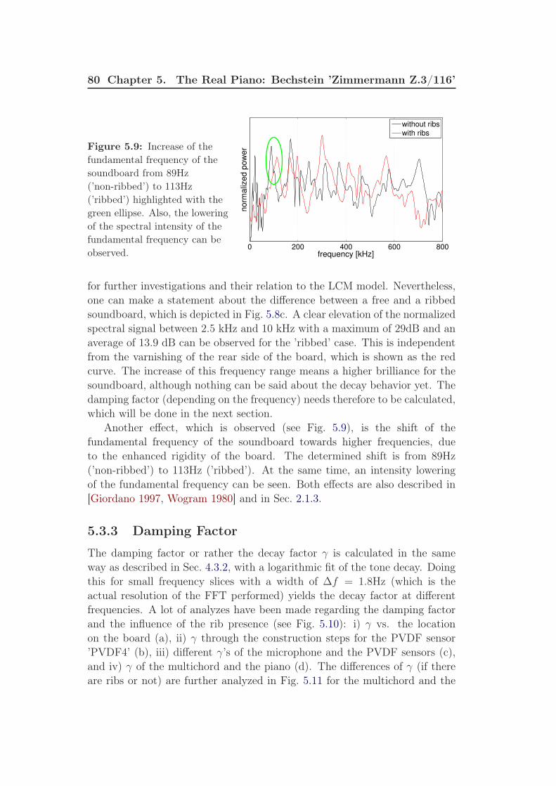
80 Chapter 5. The Real Piano: Bechstein ’Zimmermann Z.3/116’
Figure 5.9: Increase of the
fundamental frequency of the
soundboard from 89Hz
(’non-ribbed’) to 113Hz
(’ribbed’) highlighted with the
green ellipse. Also, the lowering
of the spectral intensity of the
fundamental frequency can be
observed.0 200 400 600 800
frequency [kHz]
norm
aliz
ed p
ow
er
without ribswith ribs
for further investigations and their relation to the LCM model. Nevertheless,one can make a statement about the difference between a free and a ribbedsoundboard, which is depicted in Fig. 5.8c. A clear elevation of the normalizedspectral signal between 2.5 kHz and 10 kHz with a maximum of 29dB and anaverage of 13.9 dB can be observed for the ’ribbed’ case. This is independentfrom the varnishing of the rear side of the board, which is shown as the redcurve. The increase of this frequency range means a higher brilliance for thesoundboard, although nothing can be said about the decay behavior yet. Thedamping factor (depending on the frequency) needs therefore to be calculated,which will be done in the next section.
Another effect, which is observed (see Fig. 5.9), is the shift of thefundamental frequency of the soundboard towards higher frequencies, dueto the enhanced rigidity of the board. The determined shift is from 89Hz(’non-ribbed’) to 113Hz (’ribbed’). At the same time, an intensity loweringof the fundamental frequency can be seen. Both effects are also described in[Giordano 1997, Wogram 1980] and in Sec. 2.1.3.
5.3.3 Damping Factor
The damping factor or rather the decay factor γ is calculated in the sameway as described in Sec. 4.3.2, with a logarithmic fit of the tone decay. Doingthis for small frequency slices with a width of ∆f = 1.8Hz (which is theactual resolution of the FFT performed) yields the decay factor at differentfrequencies. A lot of analyzes have been made regarding the damping factorand the influence of the rib presence (see Fig. 5.10): i) γ vs. the locationon the board (a), ii) γ through the construction steps for the PVDF sensor’PVDF4’ (b), iii) different γ’s of the microphone and the PVDF sensors (c),and iv) γ of the multichord and the piano (d). The differences of γ (if thereare ribs or not) are further analyzed in Fig. 5.11 for the multichord and the

5.3. Results 81
Bechstein soundboard.Starting with Fig. 5.10a, it can be observed that γ is not significantly
different at the rim of the soundboard both with ribs or without (see ’PVDF1’and ’PVDF6’). But in contrast to that, the middle of the soundboard (at’PVDF4’), shows a significant γ variation where the minimum changes itsposition from 2 kHz to 6.7 kHz (with a maximum variation from -50 [1/s](rib-free) to -100 [1/s] (ribbed) at about 6.7 kHz). Thus, the γ variance ofthe soundboard center is higher compared to the rim of the resonance board.The curves for one individual sensor are additionally separated by a factor of100 for a better comparison.
Fig. 5.10b shows the measurements of only one single PVDF sensor(’PVDF4’), through all the construction steps of the piano. The zoom ofthe lower part of the frequency spectra reveals a range between 1 kHz and3 kHz with a large variation of the damping factor. This frequency range,approximately beginning with the piano tone C6 (1046.50 Hz), is not onlyimportant for the higher notes, but also for the sound or rather the brillianceof the lower notes. This variability of γ for the solid-state vibrations in thisrange has not yet been reported to our knowledge. The largest γ differencewhich is at about 2 kHz corresponds to a factor of 5 between step no. 4 and5 (see Tab. 5.1). Hence, the maximum change of γ was observed when themetal frame with the strings is attached to the wooden frame of the piano.
A further analysis comprises the different acquisition techniques(condenser microphone and body vibration sensor) and their influence on thedamping factor, shown in Fig. 5.10c. Simultaneous measurements reveal largedeviations of the γ distribution dependent on the recording technique. Whileγ of the PVDF sensors shows a maximal damping around 2 kHz, the γ curvefor the condenser microphone follows a smooth decreasing trend. One of thereasons for the difference of γ between both acquisition techniques could bethe influence of the recording room on the microphone spectrum, due to lessdamping for all frequencies.
One of the most interesting parts of the analysis concerns the directcomparison of γ for the two investigated instruments (Multichord vs.Bechstein piano), which is depicted in Fig. 5.10d and Fig. 5.11. The absolutedamping factor (without ribs and with ribs) is shown in the first plot, while thelatter depicts the direct difference (’ribs’ - ’without ribs’) for each instrument.The Bechstein curves in 5.10d are enhanced by an additional factor of 100for a better comparability. Within the frequency range from 2 kHz to 8 kHzthe multichord damping factor γM reveals a slower vibrational decay with theribs mounted onto the soundboard. This results in a longer sounding of theintrument. The decay factor of the Bechstein soundboard γB has a differentoverall trend than γM , if the ribs are mounted: While in the frequency range

82 Chapter 5. The Real Piano: Bechstein ’Zimmermann Z.3/116’
0 5 10 15−200
−150
−100
−50
0
50
100
150
frequency [kHz]
dam
pin
g facto
r [1
/s]
without ribs
with ribs
0 1 2 3 4
−100
−80
−60
−40
−20
0
20
frequency [kHz]
dam
pin
g facto
r [1
/s]
without ribs
with ribs
varnishing rear side
wood frame
varnishing front
strings attached
0 2 4 6 8−100
−80
−60
−40
−20
0
frequency [kHz]
dam
pin
g facto
r [1
/s]
PVDF sensor 4
PVDF sensor 5
microphone
0 2 4 6 8
−100
−50
0
50
100
150
frequency [kHz]
dam
pin
g facto
r [1
/s]
Bechstein without ribs
Bechstein with ribs
Multichord without ribs
Multichord with ribs
(a)
PVDF 1
PVDF 4
PVDF 6
(b)
PVDF 4
(c) (d)Figure 5.10: (a): Damping factor γ for 3 different PVDF sensors (both with and
without ribs): Not many changes of γ at the rim of the soundboard, in contrast to
the middle of the board. Curves are separated by an additional factor of 100 for a
better comparability. (b): The damping factor for ’PVDF4’ excited at position
’EX 4’ followed through the assembly steps of the piano. A large parameter
variation occurs in the frequency range from about 1 kHz to 3 kHz. (c): The
difference of the damping factor between microphone and two PVDF sensor
signals. This difference is due to the different sensor technology and radiation
pattern. (Measurements after step 4 are plotted, when the rear of soundboard is
varnished (see Tab. 5.1)). (d): Bechstein vs. Multichord: Direct comparision of γ
dependent on the rib presence. Curves separated by additional factor of 100.
from 1 kHz to 3 kHz a similar behavior to the multichord can be observedwith a slower vibrational decay, the range between 3 kHz and 8 kHz showsin contrast to that a faster decay. Despite having a higher overall brilliancebetween 2.5 kHz and 10 kHz (see Fig. 5.8c), the faster vibrational decay meansa very effective radiation of the Bechstein resonance board compared to theconceptional soundboard.
The results of the investigation from [Chaigne 2011] about the rib effects
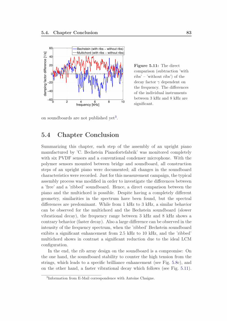
5.4. Chapter Conclusion 83
0 2 4 6 8 10−60
−40
−20
0
20
40
60
frequency [kHz]
dam
pin
g facto
r diffe
rence [1/s
]
Bechstein (with ribs − without ribs)
Multichord (with ribs − without ribs)
Figure 5.11: The direct
comparison (subtraction ’with
ribs’ – ’without ribs’) of the
decay factor γ dependent on
the frequency. The differences
of the individual instruments
between 3 kHz and 8 kHz are
significant.
on soundboards are not published yet3.
5.4 Chapter Conclusion
Summarizing this chapter, each step of the assembly of an upright pianomanufactured by ’C. Bechstein Pianofortefabrik’ was monitored completelywith six PVDF sensors and a conventional condenser microphone. With thepolymer sensors mounted between bridge and soundboard, all constructionsteps of an upright piano were documented; all changes in the soundboardcharacteristics were recorded. Just for this measurement campaign, the typicalassembly process was modified in order to investigate the differences betweena ’free’ and a ’ribbed’ soundboard. Hence, a direct comparison between thepiano and the multichord is possible. Despite having a completely differentgeometry, similarities in the spectrum have been found, but the spectraldifferences are predominant. While from 1 kHz to 3 kHz, a similar behaviorcan be observed for the multichord and the Bechstein soundboard (slowervibrational decay), the frequency range between 3 kHz and 8 kHz shows acontrary behavior (faster decay). Also a large difference can be observed in theintensity of the frequency spectrum, when the ’ribbed’ Bechstein soundboardexibits a significant enhancement from 2.5 kHz to 10 kHz, and the ’ribbed’multichord shows in contrast a significant reduction due to the ideal LCMconfiguration.
In the end, the rib array design on the soundboard is a compromise: Onthe one hand, the soundboard stability to counter the high tension from thestrings, which leads to a specific brilliance enhancement (see Fig. 5.8c), andon the other hand, a faster vibrational decay which follows (see Fig. 5.11).
3Information from E-Mail correspondence with Antoine Chaigne.
84 Chapter 5. The Real Piano: Bechstein ’Zimmermann Z.3/116’
Due to the large number of the perturbations regarding the LCM model (see2.1.4; namely the varying rib distance, the gradual thinning of the rib endings,etc.) the sound of the resonance board becomes more homogeneous. Havingthese boundary conditions, no pass-band structures, which were shown in themultichord investigation, are able to emerge. Hence, the radiation of thesoundboard is optimized in a way which is most suitable for our listeningneeds.

Chapter 6
Conclusion and Outlook
The present thesis treats the question of the generation, radiation, and thepropagation of sound waves regarding instrument soundboards. It consists oftwo parts: the development of experimental techniques in order to measureinternally propagated and radiated sound (see Chapter 3) and a comparisonof measured sound between a conceptual soundboard and a genuine Bechsteinresonance board with simple theoretical approaches (see Chapter 4 & 5).
The first part fully describes the preparation, calibration, andcharacterization of specially prepared structure-born vibration sensors, whichare made out of piezoelectric polyvinylidene fluoride (PVDF) [Kappel 2011].It is demonstrated that these special probes can be used as integrated dynamicforce sensors. The specific application of these probes for the measurementof solid-state vibrations was one of the main challenges in this investigation.The piezopolymer sensors have many practical advantages, like their variablegeometry, their flexible handling, the relatively low cost of the material, andthat they exclusively measure solid-state vibrations without perturbationsfrom airborne sound, to name just a few. The main advantage from theperspective of scientific recording, is the extremely small probe thickness,which allows minimally invasive measurements inside of a vibrating systemwith minimum perturbation. The relatively high signal-to-noise ratio andthe fast recording speed, which implies an insignificant signal delay, arecomparable to microphones.
Concerning the calibration, the relaxation of the polymer sensor underan external force was of major interest. Much effort was put into theunderstanding and the characterization of the probe efficiency both on shortand long term scales. It has been shown in this work that a careful calibrationcan compensate the impact of the parameter drift resulting from externalstress. The determination of the vertical electromechanical conversion,which is represented by the piezoelectric coefficient d33, was the importantprocedure throughout the technical part of this investigation. Its behaviorwas monitored with respect to several important parameters, such as thestatic force, the amplitude of the dynamic force, the frequency response, andthe long-term stability. Knowing these values and their evolution will yield a
86 Chapter 6. Conclusion and Outlook
reliable and calibrated measurement of the structure-born vibrations.
The second part of the study not only brought forward the applicationof these specially prepared PVDF sensors, which are mounted within musicalinstruments. Also, the investigation of scattering effects within instrumentsoundboards in the presence of a regular array are examined. The arrayconsists of uniform ribs attached to a soundboard. It was demonstrated, whichdramatic impact on the soundboard radiation and sound-wave propagationthis could have. Moreover, the acquired results and their effects can be appliedacoustically to any regularly structured surface. Only few investigations of the’ribbing’ effect of soundboards have been made [Wogram 1980, Chaigne 2011],and the obtained results are either limited in frequency range and resolution,or the results were not published yet.
The acoustic scattering effects mentioned above were investigated withtwo different setups : i) a multichord, which represents a conceptualsoundboard ([Kappel 2010]), and ii) a genuine upright piano manufactured by’C. Bechstein Pianofortefabrik’. The rectangular multichord (i) was speciallydesigned with minimal parameter variation, except for the rib mounting.Hence, a fully controllable setup was achieved, ensuring the reproducibility ofthe measured results. Governed by the question: ’What is the effect of soundwave propagation when ribs are mounted onto a soundboard?’, the number ofthe ribs as well as their distance were varied in the course of the investigation.It was found, that even just a few ribs strongly modify the sound radiation andpropagation. A banded structure of passing frequencies (and their harmonics)emerges, which can be only explained by the presence of the ribs. These ’passbands’ correspond to the eigenmodes of the structured soundboard. Theyare in perfect agreement with qualitative band theory (’linear-chain model’),analogous to the eigenmodes of phonons in solid-state physics. It was alsoobserved that the effect becomes more prominent with increasing rib number.
In addition, the assembly of an upright piano (ii) was scientificallycomplemented by mounted PVDF sensors. They were inserted between thebridge and the soundboard at the beginning of the piano build-up. Eachsingle construction step was documented, and the soundwave propagationcharacteristics of the soundboard were recorded. The traditional pianoconstruction process was modified in order to study the differences betweena ’free’ and a ’ribbed’ soundboard. Based on these results, it was possibleto make a qualitative comparison between the piano and the conceptualsoundboard. Naturally, the multichord geometry is completely different froma real piano, and thus the modal structure is much more complex for thepiano soundboard. But some similarities in the spectrum should be expected,following general arguments. Besides the fact that the additionally mounted
87
ribs in each case changed the frequency spectrum, it was found that thedamping factor γ of most Bechstein and all multichord measurements followthe same overall behavior in the frequency range from 1 to 3 kHz withhaving a minimum (i.e. the largest damping) around 2 kHz. (An exceptionrepresents the central area of the Bechstein soundboard. There, a differentbehavior concerning the damping factor γ was found, where the decay factorchanged its minimum from 2 kHz (without ribs) to 6.5 kHz (with ribs)).The spectral range from 3 to 8 kHz shows a large difference of γ betweenBechstein soundboard and multichord. While the multichord has a slowervibrational decay, the Bechstein soundboard exibits an increasing dampingfactor γ. It is clear that the different geometries and rib configurations arecausing these differences of the damping behavior. Obviously, due to thespecial design of the Bechstein piano and its deviations from the LCM model,the pass-band structure is smeared out and the radiation of the soundboardis therefore homogenized to optimize it in a way that is more suitable toour listening needs. Eventually, the specific rib design of the genuine pianocan be regarded as a compromise: The stability of the soundboard, whichis needed to withstand the high pressure generated from the strings and thespectral intensity enhancement from 3 to 10 kHz on the one hand, and onthe other hand a faster vibrational decay between 3 and 8 kHz, resultingfrom a more efficient radiation of the soundboard. The present rib designand its arrangement is the result of an evolution of the best possible listeningcharacteristics over the last three centuries.
By combining the monitoring of body vibrations with the customizedpiezoelectric PVDF sensors and the measurement of radiated airborne soundby conventional methods (e.g. condenser microphones), one is able todeduce the temporal distribution of the vibrational energy in the investigatedstructure. This acoustic recording procedure can therefore be recommendedas an optimal measurement method: PVDF sensors record the solid-statevibrations inside, and one or more condenser microphones placed outside ofthe structure acquire the airborne sound waves, simultaneously.
But many aspects concerning this topic were not yet investigated andremain open. A systematic study of the radiated and propagated sound independence on the measuring angle as well as further piezopolymer locationsfor the structure-born vibrations, could be helpful in verifying the obtainedresults. Also, the influence of different materials, geometries, and sizes for theconceptual soundboard is another starting point for follow-up measurements.But the major achievement in the future would be the exploration of the grandpiano characteristics. In particular, a long-term radiation monitoring of thesoundboard would be an interesting issue. For piano makers, the radiation
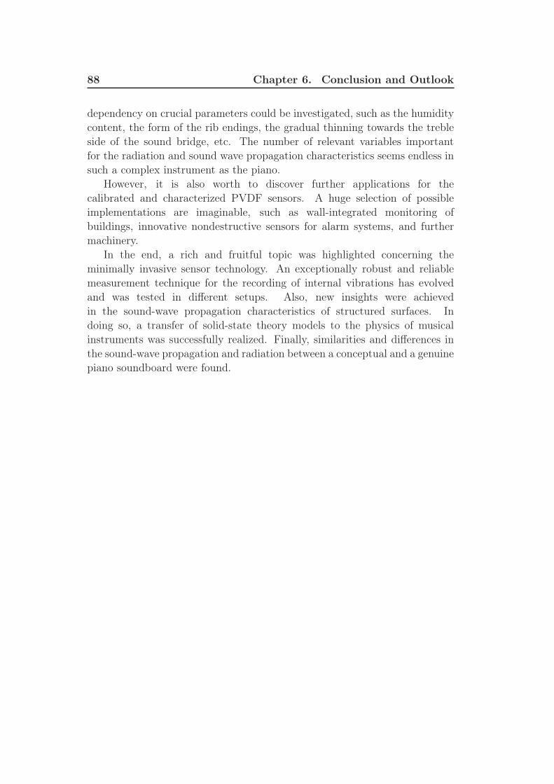
88 Chapter 6. Conclusion and Outlook
dependency on crucial parameters could be investigated, such as the humiditycontent, the form of the rib endings, the gradual thinning towards the trebleside of the sound bridge, etc. The number of relevant variables importantfor the radiation and sound wave propagation characteristics seems endless insuch a complex instrument as the piano.
However, it is also worth to discover further applications for thecalibrated and characterized PVDF sensors. A huge selection of possibleimplementations are imaginable, such as wall-integrated monitoring ofbuildings, innovative nondestructive sensors for alarm systems, and furthermachinery.
In the end, a rich and fruitful topic was highlighted concerning theminimally invasive sensor technology. An exceptionally robust and reliablemeasurement technique for the recording of internal vibrations has evolvedand was tested in different setups. Also, new insights were achievedin the sound-wave propagation characteristics of structured surfaces. Indoing so, a transfer of solid-state theory models to the physics of musicalinstruments was successfully realized. Finally, similarities and differences inthe sound-wave propagation and radiation between a conceptual and a genuinepiano soundboard were found.

Appendix A
Appendix
A.1 Technical Background
A.1.1 Microphones
The use of microphones, in particular capacitor microphones (see Fig. A.1aand b), as recording devices is a standard technique, commonly used foracoustical measurements and well described in the literature [Eargle 2004,Ballou 2009, Wong 1997].
A.1.1.1 Physical Background of Capacitor Microphones
A condenser microphone consists of one diaphragm and a backplate with asmall cavity of air (for design see Fig. A.1c). A voltage V , supplied eitherby a battery in the microphone or by external power, is applied betweenthe planes. As a further development of this concept, the electret capacitormicrophone has a special material for the diaphragm or the backplate, whichis permanently charged. Nevertheless, a preamplifier is needed in the modeof operation.The plate at the outside of the microphone, which is used as a ’diaphragm’,
is made of very light and thin material (a few microns thick). Compared todynamic microphones, the characteristics of the plate material is the reasonwhy capacitor microphones have such an outstanding frequency response,which is shown specifically for the Brüel & Kjær 1/2“ free-field microphone’type 4191’ in the next subsection (see Fig. A.2). Deformations of theouter membrane generated by a sound wave temporarily change the widthof the air cavity, resulting in a capacitance change of the charged plates.A minor distance increases the capacitance and hence a current flows,which can be measured. With an increasing distance, the capacitance isreduced and a current can be measured, too, but in the opposite direction.Therefore, a sound signal normally produces an alternating current. Capacitormicrophones are able to measure at very high audio frequencies, and they areusually much more sensitive than their dynamic counterparts. Therefore, theyrequire less amplification to produce the same level of output in comparisonto the dynamic microphones. Not only does that make them more suitable for

90 Appendix A. Appendix
(a) (b)
(c)
Figure A.1: (a): Brüel & Kjær 1/2“ free-field microphone type 4191 used for the
measurements of the airborne sound throughout this investigation.
(b): Shown is the same microphone as in (a), but with additional pre-amplifier,
which is needed for the measurements.
(c): Sketch of the condenser microphone assembly.
Figure A.2: The Brüel & Kjær 1/2“ free-field microphone ’type 4191’ frequency
response (black solid line) as given from the manufacturer.
very weak signal sources, but there is also the advantage of the linear frequencyresponse, which is an outstanding feature, de facto simplifying the process ofdata acquisition. The frequency response of the capacitor microphone is much

A.1. Technical Background 91
flatter than of the dynamic ones and therefore much easier to handle in thedata analysis.
A.1.1.2 Brüel & Kjær Condenser Microphone
Throughout this investigation the 1/2“ freefield Brüel & Kjær condensermicrophone ’type 4191’ with the preamplifier ’type 2669L’ was used. Thesignal from the microphone is then further amplified by the fitting Brüel &Kjær amplifier ’Nexus type 2690’. The frequency response function for thewhole setup, given by the manufacturer, is presented in Fig. A.2, showing aperfect flat behavior in the important frequency range 20Hz to 20kHz.
A.1.2 Acoustic Laboratory and Ambient Noise
Within the recording room, the absorption occurs at the same time as thedamping/reflection of ambient noise by the outer room walls. Consideringthe reflection, the sound wave from outside is hindered to radiate into therecording room. The damping coefficient R of a free standing wall can bedetermined theoretically by [Möser 2010]:
R ≈ 10 · lg(
ωm′′
2 · Z0
)2
, (A.1)
whereas ω, m′′ and Z0 represent the frequency, the mass of the wall in relationto its surface area and the characteristic acoustic impedance of the gas behindthe wall (which in this case is air with an impedance value of Zair = 413, 5
Ns/m3 at a temperature of 20C and a pressure of 1 atm), respectively. Thecharacteristic acoustic impedance Z0 is a material property and given by thematerial density and the sound velocity c:
Z0 = · c (A.2)
The theoretical progression of R is displayed in Fig. A.3 for three differenttemperatures (0C, 20C and 35C). It is nicely shown that there is hardly adifference in the damping coefficient R for different temperatures.
Therefore, a temperature dependence of the measurement can be safelyneglected. To measure the damping coefficient one needs two reverberationrooms – a sending room and a measurement room [Möser 2007, Veit 1996].Unfortunately, both rooms are difficult to realize for different reasons. On theone hand, the absorption material is already placed in the recording room,while on the other hand the actual acoustic laboratory is no reverberationroom at all, due to the whole measurement equipment, which acts as anabsorber. Therefore, the measurement of this characteristic is not possiblewithout destroying important parts of the recording room.

92 Appendix A. Appendix
Figure A.3: Theoretical
characteristic acoustic
impedance of the gypsum
plaster board walls of the
recording room. The sensitivity
to temperature is displayed
with three different curve
progressions. Temperatures
plotted are 0C, 20C and
35C. As can be seen from the
curves, the differences for the
three temperatures are
minimal.0 5 10 15 20
100
101
102
frequency [kHz]
dam
pin
g f
acto
r [d
B]
0°C
20°C
35°C
A.2 Additional Theoretical Background
A.2.1 Levenberg-Marquardt Method
The Levenberg-Marquardt algorithm (LMA) [Marquardt 1963] provides anumerical solution to the mathematical problem of minimizing a function,which is generally nonlinear, over a space of parameters of the function. Thisminimization problem arises especially in least-squares curve fitting. TheLMA is a modification of the Gauss-Newton algorithm (GNA), but the LMAis more robust than the GNA, which means that in many cases it generatesa solution even if the initial values are very far off the final values. Butnevertheless the convergence to a solution is not guaranteed with the LMA,due to possibly bad initial values. It could also happen, with these bad initialguesses, that the LMA just finds a local minimum and not the global one.That makes the definition of the initial guesses an important point within theprocedure.For the function F (x) : Rm → R
nm < n the minimization problem
minx∈Rm
‖F (x)‖22 (A.3)
is to be solved with the initial value x0. If it is done in the GNA, F (x) isapproximated in every step through a linearization and the alternate problem
minx∈Rm
‖F (xk) + J(xk)(x− xk)‖22 (A.4)
is observed. In that equation J represents the Jacobian of the function F .Additionally, it is required for the LMA that
‖x− xk‖22 < rk (A.5)

A.2. Additional Theoretical Background 93
Due to this additional constraint it is possible to force the decay of ‖F (xk)‖22in every step. For that the parameter rk is always adjusted.The Levenberg-Marquardt procedure descends locally to the Newtonprocedure, so the convergence is locally quadratic.
A.2.2 Correlation Function
In the data signal processing, the correlation function ξ(τ) [Smith 1997,Rodgers 1988, Hartmann 1998] between two parameters x and y is animportant mathematical method to check possible dependencies. Usualcases of ’hidden’ dependencies, for example as a function of time, spaceor temperature, will be eleminated through this function. The correlationfunction ξ(τ) of two parameters x(t) and y(t) can be written as:
ξ(τ) =
∫
∞
−∞
x(t)y(t+ τ)dt.
with ξ ∈ [−1, 1]; ξ = −1 means perfect anti-correlation, 0 no correlation atall and 1 perfect correlation. Therefore, it is needed here to normalize bothparameters in such a way, that the correlation function ξ(τ) remain in thegiven range [−1, 1]. The most practical normalization is the L2 normalization,which is defined by
‖f‖2 :=
(∫
Ω
‖f(t)‖2 dt)1/2
!= 1
Ω here represents the domain of the function. Applying the L2 normalization,ξ(τ) will always be between -1 and 1. The correlation function characterizes(similar to the transfer function) the change of shape of a wave over a timeinterval τ , or distance ∆x, respectively.
A.2.3 Fourier Transform
The Fourier transform [Smith 1997, Rabiner 1975, Guillaume 2006,Hartmann 1998] is a reversible transform of a time-dependent signalx(t) into a frequency-dependent signal x(ν). Thereby, the signal x(ν) can bedescribed bijectively as a superposition of the fundamental frequency and itsharmonics for a periodic function:
f(t) = f(t+ T0) ∀t ∈ R
and
T0 =2π
ω0
.

94 Appendix A. Appendix
where T0 represents the function period. The Fourier analysis is practical inparticular for these periodic functions.
Furthermore, x(t) needs to be continuous in the complex range and theFourier series expansion, which decomposes the periodic signals into a sum ofsimple oscillating functions, can be written as:
f(t) =∑
n∈Z
cn(f)e−inω0t ∀t ∈ R
with the respective Fourier coefficients cn(f):
cn(f) =ω0
2π
∫ π/ω0
−π/ω0
f(t)einω0tdt ∀n ∈ Z
Here, cn needs to be unique. If a complex continuous function f(t) ∈ R isfurthermore absolutely integrable (i.e. limT→∞
∫ T
−T|f(t)|dt <∞), the Fourier
transform F, which expresses the time-dependent signal x(t) as a function offrequency, will look like:
F(f(t)) =1√2π
∫
∞
−∞
f(t)e+iωtdt ∀ω ∈ R
while the back transform appears as
f(t) =1√2π
∫
∞
−∞
f(ω)e−iωtdω ∀t ∈ R
According to the Nyquist theorem [Smith 1997, Guillaume 2006], an increaseof the signal sampling rate (samples/time) will expand the frequency spectrumtowards higher frequencies. With a known sampling frequency SR, an upperfrequency bound fmax is given by: fmax < SR/2. Below this specific frequencyfmax, the whole signal can be perfectly reconstructed.
A.2.3.1 Fast Fourier Transform
The Fast Fourier transform (FFT) is the ’working horse’ in the spectralanalysis and an efficient algorithm to determine the discrete Fourier transform.The Cooley-Tukey algorithm [Cooley 1965] is the most commonly usedalgorithm. Recursively, it breaks down the discrete Fourier transform intosmaller parts, which are faster to compute. Owing to the available computingpower today, the fast Fourier transform can be done in an appropriate timespan.

A.2. Additional Theoretical Background 95
A.2.4 Tone Generation by a String
Since this investigation deals with the physics of pianos, the generation ofa tone by string vibration [Guillaume 2006] should be shortly mentioned.An ideal piano tone f(t) consist of many single sinusoidal tones, which aresuperimposed on each other:
fn(t) = An sinωnt+ ϕn, An ≥ 0, ϕn ∈ R
with T = 2πω0
as the period of the first harmonic. The lowest angularfrequency ω0 is also the smallest divisor of all frequencies concerning thistone description. This ω0, which is the fundamental frequency of the tone,is decisive for the tone pitch. The intensity distribution of the harmonics isresponsible for the tone timbre.
A.2.4.1 The 1-dim vibrating String
Generally, a string can be vibrated perpendicular (transversal) and in direction(longitudinal) of the string. The longitudinal vibration, which corresponds todensity vibrations within the string [Möser 2010], is typically not considered inthe sound analysis due to its relatively low intensity. Only accounting for thetransversal modes, it can be observed that the strings are fixed at their ends,having a velocity that equals zero – vE = 0. With these assumptions, one cansolve the one-dimensional homogeneous wave equation [Guillaume 2006]:
∂2u
∂x2− 1
c2∂2u
∂t2= 0,
with the following d’Alembert solution:
u(x, t) = ϕ(x+ ct) + ψ(x− ct)
and the two arbitrary functions ϕ and ψ, which must be differentiable.With the known boundary condition vE = 0, one obtains the followingrepresentation:
u(x, t) = asin(
2πn · xL
)
· eiωt.
This solution describes standing waves with a wave length of λ = L2n
; theseare also the only possible modes of an ideal vibrating string. Assuming thecomplete chain, which is needed to play a stringed instrument, this is of coursea very basic model. Non-linear effects, such as damping and transfer functionsthrough the instrument, are not easy to implement into the model, but theyall contribute to the individual timbre.

96 Appendix A. Appendix
A.2.5 Propagation of Sound Waves in Gases
Airborne sound waves are longitudinal waves and they can be described viathe sound wave elongation d(x, t). This is the position vector of the particleat the time t and at the position x. Under stationary condition one can statein first order, that [Möser 2007]:
rot(d(x, t)) = 0
That would mean, the rotation of the sound waves over the edge of anarea is always zero. ’Translated’ it would be: What goes in, comes out.Furthermore, one can write the vector wave equation (also in the first order)as [Guillaume 2006, Möser 2007]:
(
1
c· ∂∂t
)2
d(x, t)−∆d(x, t) = 0
with c as the sound wave velocity, fulfilling c = 1/√
〈κ〉 〈µ〉. The averagecompressibility is 〈κ〉 and 〈µ〉 represents the average density of the gas. Theseparameters are also dependent on the temperature T and the pressure p. If thesolution of the wave equation furthermore has the condition rot(d(x, t)) = 0,the solutions will be longitudinal waves.
In the following some other important parameters for the propagation ofsound waves, which can also be found in [Guillaume 2006, Möser 2007], arepresented. First of all, there is the sound particle velocity, which is describedby the sound-wave displacement:
u(x, t) =∂
∂td(x, t)
Secondly, the sound pressure p = P − 〈P 〉 can also be defined via thesound-wave displacement:
p(x, t) = − 1
〈κ〉div(d(x, t))
The sound wave velocity is dependent on the temperature:
c(T ) ≈√
T
T0c(T0)
where T0 = 273, 15 K. Therefore, the velocity of the sound wave increases forhigher temperatures. That is due to the larger mobility of the sound particlesand arises from thermodynamics.

A.2. Additional Theoretical Background 97
Figure A.4: (Graph taken from
[Hillenbrand 2004].) The resonance
spectrum of cellular polypropylene
with a thickness of 70µm. At
300kHz, the thickness resonance
and a significant enhancement of
the piezoelectric coefficient d33 can
be seen.
A.2.6 Resonance Spectrum
The resonance can be described by the behavior of a system to oscillateat different amplitudes for different frequencies. Where the oscillatingamplitudes become locally and/or globally large, resonance occurs; namely atthe resonance frequencies. Even very small driving forces could then lead toresonance catastrophe, because the system stores to much of the vibrationalenergy. The vibrational intensity I for a specific resonance frequency ω0 isgiven through the formula [Hartmann 1998]:
I(ω) ∝ 1
|(1− ( ωω0)2)|
where ω means the driving frequency. In Fig. A.4 the behavior of a thinpolymer film under an external driving voltage is shown as an example for aresonance spectrum.
A.2.7 Signal-to-Noise Ratio
The signal-to-noise ratio (SNR) [Smith 1997, Hartmann 1998,Guillaume 2006] is a measure for the quality of a signal, which is overlayedby noise. It is defined by the ratio of the average power of the signal to thatof the noise source:
SNR =PS
PN
while the power is defined via the effective voltage being the root mean squareof the time varying value:
SNRdB = 10 lg
(
PS
PN
)
= 10 lg
(
u2eff,Su2eff,N
)
.
98 Appendix A. Appendix
Figure A.5: Figure taken
from [Russell 1998].
Radiation characteristics of
an acoustic dipole at 250
Hz.
Moreover, one can define the SNR in [dB] by:
SNRdB = 20 lg
(
Var(Signal)
Var(Noise)
)
Simply by the determination of the variances (the measure of the averagedistance of an random value to its expected value), the SNR [dB] can alsobe reconstructed. With the help of these equations, the SNR of the speciallyprepared piezopolymer can be determined with SNRdB = 78dB measured atthe first harmonic of the multichord.
A.2.8 Acoustic Dipole Radiation
An acoustic dipole can be associated as two monopole sources [Russell 1998],which have an opposite phase and equal strength. The dipole radiates nothomogeneously. There is a specific directivity (see Fig. A.5), which is alsofrequency-dependent compared to the monopole [Russell 1998].
A.2.9 Impedance
Generally, two kinds of impedances can be distinguished: the electrical andthe acoustical or rather the specific mechanical impedance.
A.2. Additional Theoretical Background 99
A.2.9.1 Acoustic Impedance
The acoustical impedance [Morse 1936, Veit 1996, Möser 2010, Bucur 2006,Giordano 1998a] in the free sound field is the multiplication of density andlongitudinal velocity vc and describes the resistance against the propagatingsound wave:
Za = · vc (A.6)
Within a material, the acoustical impedance can be represented by thematerial constants: sound-wave pressure p and sound-wave flux q:
Za =p
q
A.2.9.2 Electrical Impedance
Since the sound vibrations in this investigation are always electricallyrecorded, it is worth to take a look at the electrical impedance ze[Alexander 2006], because every change of the conducting material will changeze. This will result in additional reflections at the junctions, which will bepresent in the frequency spectrum. But these device effects can be deconvolvedfrom the measured signal in order to have a ’device function’-free spectrum.
The electrical impedance ze, which is also called the alternating current(AC) resistance, is the quotient of the complex alternating voltage u and thecomplex alternating current i:
ze =u
i.
But ze can also be expressed by the active resistance R and the reactance X:
ze = R + i ·X.with i as the imaginary unit. X is dependent on the frequency: either itruns ahead (concerning the inductivity of a coil) or behind (concerning thecapacitance of a condensor) a signal. Therefore, in the present case, wherethe measurements were performed with a cable (with a condensor setup), Xis running behind the signal and can be expressed with:
Z = |Z| · expiϕ .
φ is here the phase angle. The absolute value of the apparent impedance Z isgiven by the effective values of the voltage and the current:
Z =Ueff
Ieff
The ideal setup for electrical recordings to avoid reflections at the transitionpoints can be summarized with: input resistance Ri equals output resistanceRo.
100 Appendix A. Appendix
A.2.10 Sound Pressure Quantity
An average human ear can withstand a sound pressure of ∼ 20Pa before itgets damaged [Veit 1996], which is about 106 times the threshold of humanhearing (p0 = 2·10−5Pa at 1000Hz). Due to its wide range, the sound pressureLp is commonly given on logarithmic scale [Veit 1996, Möser 2007]:
Lp =def 20 · log10
(
p
p0
)
[dB] (A.7)
p represents the effective sound pressure and is given through the maximumvalue of the sound pressure: ⇒ p = pmax/
√2. For example, a normal
conversation at a distance of 1m has a sound pressure of about Lp = 1µbar= 74 dB.Giving the sound-wave energy density ρ(x, t):
ρ(x, t) =def〈κ〉2
(
∂
∂td(x, t)
)2
+1
2〈κ〉(div(d(x, t)))2 (A.8)
and the sound intensity or the energy flux density of the sound wave (x, t):
(x, t) =def p(x, t)u(x, t) (A.9)
the continuity equation is then given by:
∂
∂tρ+ div = 0 (A.10)

Appendix B
Curriculum Vitæ
Personal Data
Name: Marcel Kappel
Birth: 02.12.1981 in Nauen
Address: An der Petersburg 8, 49082 Osnabrück
Email: [email protected]
Education
Aug. 2008 – present Member of Research Staff; PhD-Thesis at theACMP Group (University Potsdam) under theSupervision of Prof. R. Gerhard
Oct. 2006 – Nov. 2007 Diploma Thesis at the Astrophysical Institute ofPotsdam
Oct. 2002 – Mar.2008
Study of Physics at the University of Potsdam
July 2001 – Apr. 2002 Civil Service at the Office for Environment inKetzin
June 2001 ’Abitur’ at the ’Goethe-Gymnasium’ in Nauen
June 1998 ’Mittlere Reife’ at the Comprehensive School inKetzin
102 Appendix B. Curriculum Vitæ
Employment & Practical Experience
2009 – 2012 4 Contributions at the Long Night of Science
2008 – 2011 5 Semester of weekly Tutorials for ExperimentalPhysics
2008 – 2010 Participation in the Project: SEPHA –Didaktische Konzepte für die strukturierteStudieneingangsphase
March – August 2006 Student Assistant for the Maintaining of a DataReduction Pipeline
Publications
2010 M. Kappel, M. Abel und R. Gerhard’Sound Generation in a Piano: Multichannel
Measurements’ Conference Proceedings ’DAGA2010’
2010 M. Kappel, M. Abel und R. Gerhard ’Comparison
of Measurements on a Simplified Piano Model
with a Condenser Microphone and a Piezoelectric
Polymer Sensor’ Conference Proceedings ’DAGA2011’
2011 M. Kappel, M. Abel und R. Gerhard’Characterization and Calibration of Piezoelectric
Polymer: in-situ Measurements of Body
Vibrations’ Rev. Sci. Instrum. 82, 075110(2011)
2012 Co-Author of a Chapter in: Kossak, Peter;Lehmann, Uta; Ludwig, Joachim (Ed.) ’Die
Studieneingangsphase - Analyse, Gestaltung und
Entwicklung.’ (ISBN-10: 3937026770)
103
Conference Contributions
2010 DAGA 2010 Berlin, Poster: ’Sound Generation
in a Piano: Multichannel Measurements’
2011 DPG 2011 Dresden, Poster: ’Acoustic
Calibration and Characterization of PVDF: in-situ
Measurements of Body Vibrations’
2011 DAGA 2011 Düsseldorf, Oral Prasentation:’Scattering Effects: Ribs on Soundboard’

Bibliography
[Alexander 2006] C. Alexander and M. Sadiku. Fundamentals of electriccircuits. McGraw-Hill; 3. revised edition, 2006.
[Altafim 2009] R. A. P. Altafim, X.Qiu, W. Wirges, R. Gerhard,R. A. C. Altafim, H. C. Basso, W. Jenninger and J. Wagner.Template-based fluoroethylenepropylene piezoelectrets with tubular
channels for transducer applications. J. Appl. Phys, vol. 106, 2009.
[Ashcroft 1976] N. W. Ashcroft and N. D. Mermin. Solid state physics. BrooksCole, 1976.
[Askenfelt 1993] A. Askenfelt and E. V. Jansson. From touch to string
vibrations. I to III. J. Acoust. Soc. Am., 1990 –1993.
[Ballou 2009] G. Ballou. Electroacoustic devices: Microphones andloudspeakers. Focal Press, 2009.
[Bauer 2004] S. Bauer, R. Gerhard-Multhaupt and G. M. Sessler.Ferroelectrets: Soft Electroactive Foams for Transducers. PhysicsToday, vol. 57 (2), pages 37–43, 2004.
[Bayer 1993] G. Bayer and T. Niederdränk. Weak localization of acoustic
waves in strongly scattering media. Phys. Rev. Lett., vol. 70, pages3884–3887, 1993.
[Bechstein 2005] C. Bechstein. The world of pianos - fascination with aninstrument. Nicolai-Verlag, 2005.
[Bensa 2003] J. Bensa, S. Bilbao, R. Kronland-Martinet and J. O. Smith.The simulation of piano string vibration: From physical models to
finite difference schemes and digital waveguides. J. Acoust. Soc. Am.,vol. 114, pages 1095–1107, aug 2003.
[Bensa 2005] J. Bensa, O. Gipouloux and R. Kronland-Martinet. Parameter
fitting for piano sound synthesis by physical modeling. J. Acoust. Soc.Am., vol. 118, pages 495–504, jul 2005.
[Bissinger 2008] G. Bissinger. Structural acoustics of good and bad violins. J.Acoust. Soc. Am., vol. 124, pages 1764–1773, 2008.
[Bork 1993] I. Bork. Abstrahlung des Anschlaggeräuschs beim Flügel. Berichtder 17. Tonmeistertagungen, pages 751–764, 1993.

106 Bibliography
[Bucur 2006] V. Bucur. Acoustics of wood. Springer, 2006.
[Chaigne 1994a] A. Chaigne and A. Askenfelt. Numerical simulations of piano
strings. I. A physical model for a struck string using finite difference
methods. J. Acoust. Soc. Am., vol. 95, pages 1112–1118, feb 1994.
[Chaigne 1994b] A. Chaigne and A. Askenfelt. Numerical simulations of piano
strings. I and II. J. Acoust. Soc. Am., 1994.
[Chaigne 1994c] A. Chaigne and A. Askenfelt. Numerical simulations of
piano strings. II. Comparisons with measurements and systematic
exploration of some hammer-string parameters. J. Acoust. Soc. Am.,vol. 95, pages 1631–1640, mar 1994.
[Chaigne 2011] A. Chaigne, R. Vuillez and R. Viggiano. Influence of ribs on
the radiation of a piano soundboard. In Proceedings: 161st Meeting:Acoustical Society of America, Aspen, USA, 2011.
[Condat 1986] C. A. Condat and T. R. Kirkpatrick. Localization and resonant
transmission of third-sound waves on a random substrate. Phys. Rev.B, vol. 33, pages 3102 – 3114, 1986.
[Conklin Jr. 1990] H. A. Conklin Jr., A. Askenfelt, E. Janson, D. E. Hall,G. Weinreich and K. Wogram. Five lectures on the acoustics of the
piano, 1990. Royal Swedish Academy of Music ISBN-10: 9185428620.
[Conklin Jr. 1996a] H. A. Conklin Jr. Design and tone in the mechanoacoustic
piano. Part I. Piano hammers and tonal effects. J. Acoust. Soc. Am.,vol. 99, pages 3286–3296, jun 1996.
[Conklin Jr. 1996b] H. A. Conklin Jr. Design and tone in the mechanoacoustic
piano. Part I to III. J. Acoust. Soc. Am., 1996.
[Conklin Jr. 1996c] H. A. Conklin Jr. Design and tone in the mechanoacoustic
piano. Part II. Piano structure. J. Acoust. Soc. Am., vol. 100, pages695–708, aug 1996.
[Conklin Jr. 1996d] H. A. Conklin Jr. Design and tone in the mechanoacoustic
piano. Part III. Piano strings and scale design. J. Acoust. Soc. Am.,vol. 100, pages 1286–1298, sep 1996.
[Cooley 1965] J. W. Cooley and J. W. Tukey. An algorithm for the machine
calculation of complex Fourier series. Math. Comput., vol. 19, no. 90,pages 297 – 301, 1965.

Bibliography 107
[Crisanti 1993] A. Crisanti, G. Paladin and A. Vulpiani. Products of randommatrices in statistical physics, pages pp. 87–115. Springer Series inSolid-State Sciences, 1993.
[Curie 1880] J. Curie and P. Curie. Développement par compression de
l’électricité polaire dans les cristaux hémièdres à faces inclinées. Bull.Soc. Min. France, pages 90 – 93, 1880.
[Das-Gupta 1991] D. K. Das-Gupta. Pyroelectricity in Polymers.Ferroelectrics, vol. 118, pages 165 – 189, 1991.
[Dickens 1992] B. Dickens, E. Balizer, A. S. DeReggi and S. C. Roth.Hysteresis measurements of remanent polarization and coercive field
in polymers. J. Appl. Phys., vol. 72, pages 4258 – 4264, 1992.
[DIN e.V. 2005a] DIN e.V. Akustik - Messung der Schalldämmung inGebäuden und von Bauteilen - Teil 1 (DIN EN ISO 140-1). BeuthVerlag GmbH, 2005.
[DIN e.V. 2005b] DIN e.V. Akustik - Messung der Schalldämmung inGebäuden und von Bauteilen - Teil 3 (DIN EN ISO 140-3). BeuthVerlag GmbH, 2005.
[DIN e.V. 2010] DIN e.V. Bestimmung der Schallleistungs- undSchallenergiepegel von Geräuschquellen aus Schalldruckmessungen(DIN EN ISO 3745). Beuth Verlag GmbH, 2010.
[Ducasse 2005] E. Ducasse. On waveguide modeling of stiff piano strings. J.Acoust. Soc. Am., vol. 118, pages 1776–1781, sep 2005.
[Eargle 2004] J. Eargle. The microphone book, second edition: From monoto stereo to surround - a guide to microphone design and application.Focal Press, 2004.
[Elejabarrieta 2002] M. J. Elejabarrieta, A. Ezcurra and C. Santamaria.Coupled modes of the resonance box of the guitar. J. Acoust. Soc.Am., vol. 111, pages 2283–2292, may 2002.
[Filippi 1999] P. Filippi, D. Habault, J. P. Lefebvre and A.Bergassoli.Acoustics: Basic physics, theory and methods. Academic Press, 1999.
[Fletcher 1993] N. H. Fletcher and T. D. Rossing. The physics of musicalinstruments. Springer-Verlag, 1993.

108 Bibliography
[Fletcher 1999] N. H. Fletcher. The nonlinear physics of musical instruments.Rep. Prog. Phys., vol. 62, pages 723–764, may 1999.
[Fukada 1950] E. Fukada. Vibrational study of the wood used for the sound
boards of pianos. Nature, vol. 166, pages 772 – 773, 1950.
[Furukawa 1981] T. Furukawa, G. E. Johnson, H. E. Bair, Y. Tajitsu,A. Chiba and E. Fukada. Ferroelectric Phase Transition
in a Copolymer of Vinylidene Fluoride and Trifluoroethylene.Ferroelectrics, vol. 32, pages 61 – 67, 1981.
[Furukawa 2001] T. Furukawa and Y. Takahashi. Ferroelectric and
antiferroelectric transitions in random copolymers of vinylidene
fluoride and trifluoroethylene. Ferroelectrics, vol. 264, page 1739, 2001.
[Giordano 1996] N. Giordano and A. J. Korty. Motion of a piano string:
Longitudinal vibrations and the role of the bridge. J. Acoust. Soc.Am., vol. 100, pages 3899–3908, dec 1996.
[Giordano 1997] N. Giordano. Simple model of a piano soundboard. J. Acoust.Soc. Am., vol. 102, pages 1159–1168, aug 1997.
[Giordano 1998a] N. Giordano. Mechanical impedance of a piano soundboard.J. Acoust. Soc. Am., vol. 103, pages 2128–2133, apr 1998.
[Giordano 1998b] N. Giordano, H. Gould and J. Tobochnik. The physics of
vibrating strings. Comput. Phys., vol. 12, pages 138–145, mar 1998.
[Giordano 2006] B. Giordano and S. McAdams. Material identification of
real impact sounds: Effects of size variation in steel, glass, wood and
plexiglass plates. J. Acoust. Soc. Am., vol. 119, pages 1171–1181, feb2006.
[Goldstein 1980] H. Goldstein. Classical mechanics. Addison-WesleyPublishing Company, 1980.
[Gren 2006] P. Gren, K. Tatar, J. Granström, N. E. Molin and E. V. Jansson.Laser vibrometry measurements of vibration and sound fields of a bowed
violin. Measur. Sci. Technol., vol. 17, pages 635–644, apr 2006.
[Guillaume 2006] P. Guillaume. Music and acoustics. ISTE Ltd, London,2006.
Bibliography 109
[Hahn 1985] B. Hahn and J. Wendorff. Dielectric relaxation of the
crystal-amorphous interphase in poly (vinylidene fluoride) and its
blends with poly (methyl methacrylate). Macromolecules, vol. 18, pages718 – 721, 1985.
[Hall 1992a] D. E. Hall. Piano string excitation I to VI (series). J. Acoust.Soc. Am., 1987-1992.
[Hall 1992b] D. E. Hall. Piano string excitation. VI: Nonlinear modeling. J.Acoust. Soc. Am., vol. 92, pages 95–105, jul 1992.
[Harrison 2001] J. S. Harrison and Z. Ounaies. Piezoelectric Polymers. ICASEReport, no. 2001-43, 2001.
[Hartmann 1998] W. Hartmann. Signals, sound, and sensation. Springer,1998.
[Hayashi 1999] E. Hayashi, M. Yamane and H. Mori. Behavior of piano-action
in a grand piano. I. Analysis of the motion of the hammer prior to
string contact. J. Acoust. Soc. Am., vol. 105, pages 3534–3544, jun1999.
[Hillenbrand 2004] J. Hillenbrand and G. M. Sessler. Quasistatic and
Dynamic Piezoelectric Coefficients of Polymer Foams and Polymer
Film Systems. IEEE Transactions on Dielectrics and ElectricalInsulation, vol. 11, pages 72 – 79, 2004.
[Kappel 2010] M. Kappel, M. Abel and R. Gerhard. The effect of Mounted
Ribs on the Radiation of a Soundboard. arXiv:1011.5372v1, 2010.
[Kappel 2011] M. Kappel, M. Abel and R. Gerhard. Characterization and
calibration of piezoelectric polymers: In situ measurements of body
vibrations. Rev. Sci. Instrum., vol. 82, page 075110, 2011.
[Kawai 1969] H. Kawai. The piezoelectricity of polyvinylidene fluoride. Jpn.J. Appl. Phys., vol. 8, pages 975–976, 1969.
[Kittel 1953] C. Kittel. Introduction to solid state physics. Wiley, 1953.
[Komano 1994] T. Komano and T. Kunimoto. Electronic musical instrument
which simulates physical interaction of piano string and hammer. J.Acoust. Soc. Am., vol. 96, page 621, jul 1994.
[Kremmer 2007] A. Kremmer. Untersuchungen der Struktur von Polyamid11-Filmen und ihres Einflusses auf deren piezo- und ferroelektrischenEigenschaften, pages 16 – 23. PhD thesis (in german), 2007.

110 Bibliography
[Kressmann 2001] R. Kressmann. Linear and Nonlinear Piezoelectric
Response of Charged Cellular Polypropylene. J. Acoust. Soc. Am.,vol. 104, pages 3489 – 3496, 2001.
[Kulek 2002] J. Kulek, Cz. Pawlaczyk and E. Markiewicz. Influence of poling
and ageing on high-frequency dielectric and piezoelectric response of
PVDF-type polymer foils. Journal of Electrostatics, vol. 56, pages 135– 141, 2002.
[Künstler 2000] W. Künstler, Z. Xia, T. Weinhold, A. Pucherand R. Gerhard-Multhaupt. Piezoelectricity of porous
polytetrafluoroethylene single- and multiple-film electrets containing
high charge densities of both polarities. Appl. Phys. A, vol. 70, no. 1,pages 5 – 8, 2000.
[Landolt 2006] H. Landolt and R. Börnstein. Ferroelectrics and relatedsubstances. Springer, 2006.
[Mamou-Mani 2008] A. Mamou-Mani, J. Frelat and C. Besnainou. Numerical
simulation of a piano soundboard under downbearing. J. Acoust. Soc.Am., vol. 123, pages 2401–2406, 2008.
[Marquardt 1963] D. W. Marquardt. An algorithm for least squares
estimation of nonlinear parameters. SIAM J. Appl. Math., vol. 11,pages 431 – 441, 1963.
[Mellinger 2003] A. Mellinger. Dielectric Resonance Spectroscopy: a Versatile
Tool in the Quest for Better Piezoelectric Polymers. IEEE Transactionson Dielectrics and Electrical Insulation, vol. 10, pages 842 – 861, 2003.
[Moore 2006] T. R. Moore and S. A. Zietlow. Interferometric studies of a
piano soundboard. J. Acoust. Soc. Am., vol. 119, pages 1783–1793,2006.
[Morse 1936] P. M. Morse. Vibration and sound. AIP for ASA, 1936.
[Morse 1987] P. M. Morse and K. U. Ingard. Theoretical acoustics, pages pp.175–227. Princeton University Press, 1987.
[Möser 2007] M. Möser. Technische Akustik. Springer, 2007.
[Möser 2010] M. Möser and W. Kropp. Körperschall. Springer, 2010.
Bibliography 111
[MSI 2006] Measurements Specialities, Inc. MSI. Piezo
Film Sensors – Technical Manual, 2006.http://www.media.mit.edu/resenv/classes/MAS836/Readings/MSI-techman.pdf.
[Newman 1980] B. A. Newman, P. Chen, K. D. Pae and J. I. Scheinbeim.Piezoelectricity in Nylon-11. J. Appl. Phys., vol. 51 (10), pages 5161– 5164, 1980.
[Nix 1986] E. L. Nix and I. M. Ward. The measurement of the shear
piezoelectric coefficients of polyvinylidene fluoride. Ferroelectrics,vol. 67, pages 137 – 141, 1986.
[Oshiki 1976] M. Oshiki and E. Fukada. Piezoelectric Effect in Stretched and
Polarized Polyvinylidene Fluoride Film. Jpn. J. Appl. Phys., vol. 15,pages 43 – 52, 1976.
[Parakilas 1999] J. Parakilas. Piano roles: Three hundred years of life withthe piano. Yale University Press, 1999.
[Pollens 1995] S. Pollens. The early pianoforte. Cambridge University Press,1995.
[Pu 2010] J. Pu, X. Yan, Y. Jiang, C. Chang and L. Lin. Piezoelectric
actuation of direct-write electrospun fibers. Sensors and Actuators A,vol. 164, pages 131 – 136, 2010.
[Rabiner 1975] L. R. Rabiner and B. Gold. Theory and application of digitalsignal processing. Englewood Cliffs, N.J., Prentice-Hall, Inc., 1975.
[Rodgers 1988] J. L. Rodgers and W. A. Nicewander. Thirteen ways to look
at the correlation coefficient. Am. Statist., vol. 42, pages 59–66, 1988.
[Rollik 1999] D. Rollik, S. Bauer and R. Gerhard-Multhaupt. Separate
contributions to the pyroelectricity in polyvinylidene fluoride from the
amorphous and crystalline phases as well as their interfaces. J. Appl.Phys., vol. 85, pages 3282 – 3288, 1999.
[Russell 1998] D. A. Russell, J. P. Titlow and Y.-J. Bemmen. Acoustic
monopoles, dipoles, and quadrupoles: An experiment revisited. Am.J. Phys., vol. 67, pages 660 – 664, 1998.
[Schuck 1943] O. H. Schuck and R. W. Young. Observations on the Vibrations
of Piano Strings. J. Acoust. Soc. Am., vol. 15, pages 1–11, 1943.
112 Bibliography
[Sessler 1981] G. M. Sessler. Piezoelectricity in polyvinylidenefluoride. J.Acoust. Soc. Am., vol. 70 (6), pages 1596 – 1608, 1981.
[Sessler 1999a] G. M. Sessler and R. Gerhard-Multhaupt. Electrets, ThirdEdition in two Volumes, 1999.
[Sessler 1999b] G. M. Sessler and R. Gerhard-Multhaupt. Electrets, thirdedition in two volumes, cap. Laplacian Press, Morgan Hill, CA, 1999.
[Smith 1997] S. W. Smith. The Scientist and Engineer’s Guide to Digital
Signal Processing, 1997. ISBN-10: 0966017633.
[Suzuki 1986] H. Suzuki. Vibration and sound radiation of a piano
soundboard. J. Acoust. Soc. Am., vol. 80, pages 1573–1582, dec 1986.
[Suzuki 1987] H. Suzuki. Model analysis of a hammer-string interaction. J.Acoust. Soc. Am., vol. 82, pages 1145–1151, oct 1987.
[Suzuki 2007] H. Suzuki. Spectrum analysis and tone quality evaluation of
piano sounds with hard and soft touches. Acoust. Sci. Techn., vol. 28,pages 1–6, 2007.
[Takahashi 1987] Y. Takahashi, M. Iijima, K. Inagawa and A. Itoh. Synthesis
of Aromatic Polyamide Film by Vacuum Deposition Polymerization.J. Vac. Sci. Technol. A, vol. 5, page 2253, 1987.
[Takahashi 1989] Y. Takahashi, M. Iijima and E. Fukada. Pyroelectricity in
Poled Thin Films of Aromatic Polyurea Prepared by Vapor Deposition
Polymerization. Jpn. J. Appl. Phys., vol. 28, pages L408 – L410, 1989.
[Tanaka 1996] H. Tanaka, K. Mizutani and K. Nagai. Two-dimensional
motion of a single piano string. J. Acoust. Soc. Am., vol. 100, page2843, oct 1996.
[Tasaka 1981] S. Tasaka and S. Miyata. The origin of piezoelectricity in
poly(vinylidene fluoride). Ferroelectrics, vol. 32, pages 17–23, 1981.
[Tashiro 1981] K. Tashiro, H. Tadokoro and M. Kobayashi. Structure and
piezoelectricity of poly(vinylidene fluoride). Ferroelectrics, vol. 32, page167, 1981.
[The MathWorks, Inc. ] The MathWorks, Inc. MATLAB - The Language Of
Technical Computing.
[Tufillaro 1989] N. B. Tufillaro. Nonlinear and chaotic string vibrations. Am.J. Phys., vol. 57, pages 408–414, may 1989.
Bibliography 113
[Tufillaro 1995] N. B. Tufillaro, P. Wyckoff, R. Brown, T. Schreiber andT. Molteno. Topological time series analysis of a string experiment and
its synchronized model. Phys. Rev. E, vol. 51, no. 1, pages 164–174,1995.
[v. Helmholtz 1863] H. v. Helmholtz. Die Lehre von Tonempfindungen alsphysiologische Grundlage für die Theorie der Musik. Friedrich Viewegund Sohn, 1863.
[Veit 1996] I. Veit. Technische Akustik. Vogel Fachbuch; Kamprath-Reihe,1996.
[Vinogradov 2002] A. Vinogradov and M. Schwartz. Piezoelectricity inpolymers, pages 780 – 792. Encyclopedia of Smart Materials, Volumes1-2. John Wiley and Sons, 2002.
[Vyasarayani 2009] C. P. Vyasarayani, S. Birkett and J. McPhee. Modeling the
dynamics of a compliant piano action mechanism impacting an elastic
stiff string. J. Acoust. Soc. Am., vol. 125, pages 4034–4042, 2009.
[Wada 1981] Y. Wada and R. Hayakawa. A Model of Piezo- and
Pyroelectricity of Poly(Vinylidene Fluoride) Electret. Ferroelectrics,vol. 32, pages 115 – 118, 1981.
[Weinreich 1977] G. Weinreich. Coupled piano strings. J. Acoust. Soc. Am.,vol. 62, pages 1474–1484, dec 1977.
[Wogram 1980] K. Wogram. Acoustical Research on Pianos: Vibrational
Characteristics of the Soundboard. Das Musikinstrument, vol. 24, pages694–702, 1980.
[Wong 1997] G. S. K. Wong and T. F. W. Embleton. AIP handbook ofcondenser microphones: Theory, calibration and measurements. AIPSeries in Modern Acoustics and Signal Processing. Springer, Berlin,1997.
[Yoshikawa 2007] S. Yoshikawa. Acoustical classification of woods for string
instruments. J. Acoust. Soc. Am., vol. 122, pages 568–573, 2007.
[Young 1952] R. W. Young. Inharmonicity of Plain Wire Piano Strings. J.Acoust. Soc. Am., vol. 24, pages 267–273, 1952.
[Zhang 2002] Q. M. Zhang, V. Bharti, G. Kavarnos and M. Schwartz.Poly(vinylidene fluoride) (PVDF) and its copolymers, pages 807–825.

114 Bibliography
Encyclopedia of Smart Materials, Volumes 1-2. John Wiley and Sons,2002.
[Ziman 1972] J. Ziman. Principles of the theory of solids. CambridgeUniversity Press, 1972.
List of Figures
2.1 The upright and the grand piano. . . . . . . . . . . . . . . . . 62.2 Cross Section of a Piano . . . . . . . . . . . . . . . . . . . . . 82.3 Piano Soundboard Modes . . . . . . . . . . . . . . . . . . . . 102.4 Mechanical impedance of a soundboard (numeric solution) . . 112.5 Dispersion relation of the LCM model . . . . . . . . . . . . . . 132.6 Born-von Karman boundary condition . . . . . . . . . . . . . 152.7 Theoretical dispersion relation . . . . . . . . . . . . . . . . . . 162.8 Stress Tensor Components . . . . . . . . . . . . . . . . . . . . 172.9 Chemical formula of PVDF . . . . . . . . . . . . . . . . . . . 192.10 PVDF morphology . . . . . . . . . . . . . . . . . . . . . . . . 202.11 Poling Process for the PVDF . . . . . . . . . . . . . . . . . . 21
3.1 Photos of the recording room + absorption material . . . . . . 253.2 Sound pressure measured at different distances to the loudspeaker 273.3 Sound pressure quotient with/without floor metal grid . . . . 283.4 Reverberation Time Determination . . . . . . . . . . . . . . . 293.5 Plotted Reverberation Time . . . . . . . . . . . . . . . . . . . 313.6 Sputtering setup . . . . . . . . . . . . . . . . . . . . . . . . . 323.7 Preparation steps for the PVDF sensors . . . . . . . . . . . . 333.8 Dynamic force measurement setup . . . . . . . . . . . . . . . . 363.9 d33-coefficient vs. initial force and d33 coefficient vs. dynamical
force . . . . . . . . . . . . . . . . . . . . . . . . . . . . . . . . 383.10 d33-coefficient short and long term evolution . . . . . . . . . . 413.11 PVDF frequency response . . . . . . . . . . . . . . . . . . . . 43
4.1 Multichord picture and overview . . . . . . . . . . . . . . . . . 514.2 Multichord overview sketch . . . . . . . . . . . . . . . . . . . 524.3 Spectrum: rib effects (13 ribs – 0 ribs) . . . . . . . . . . . . . 544.4 Direct comparison: PVDF vs. microphone spectrum . . . . . . 554.5 Different excitation points at the multichord . . . . . . . . . . 564.6 The most important longitudinal modes of the investigated
multichord. . . . . . . . . . . . . . . . . . . . . . . . . . . . . 574.7 Shifted pass bands of the multichord . . . . . . . . . . . . . . 594.8 Rib effect: successive rib mountening . . . . . . . . . . . . . . 604.9 Equal rib number with different rib distances . . . . . . . . . . 614.10 Time dependent frequency spectrum – PVDF and microphone 614.11 Damping factor algorithm . . . . . . . . . . . . . . . . . . . . 62

116 List of Figures
4.12 Damping factor for different rib numbers . . . . . . . . . . . . 634.13 Fitting the theoretical peaks of the pass band to the recorded
data . . . . . . . . . . . . . . . . . . . . . . . . . . . . . . . . 644.14 Comparing theoretical and experimental pass band peaks . . . 654.15 The different dispersion relations between the various rib
distances. . . . . . . . . . . . . . . . . . . . . . . . . . . . . . 66
5.1 Piano ’Zimmermann Z.3/116 ’ . . . . . . . . . . . . . . . . . . 705.2 Process of the PVDF mounting in the piano . . . . . . . . . . 725.3 Design drawing of the Bechstein ’Z.3/116’ soundboard and
resonance board pictures (front and back) . . . . . . . . . . . 745.4 Steps in the constructing of the upright piano – part 2 (Until
the strings are placed.) . . . . . . . . . . . . . . . . . . . . . . 755.5 Repeatability of the excitation mechanism . . . . . . . . . . . 765.6 Location of the maximal amplitudes . . . . . . . . . . . . . . . 765.7 Pulse amplitudes for all PVDF sensors and all sessions . . . . 775.8 Spectra form the Bechstein Sessions . . . . . . . . . . . . . . . 795.9 Change of the fundamental frequency of the ’non-ribbed’ and
’ribbed’ soundboard . . . . . . . . . . . . . . . . . . . . . . . . 805.10 Frequency depending damping factors for the Bechstein
soundboard . . . . . . . . . . . . . . . . . . . . . . . . . . . . 825.11 Direct comparison of the decay factors between the multichord
and the Bechstein soundboard. . . . . . . . . . . . . . . . . . 83
A.1 Condenser microphone (picture & sketch) . . . . . . . . . . . . 90A.2 Brüel & Kjær 1/2“ free-field microphone ’type 4191’ frequency
response. . . . . . . . . . . . . . . . . . . . . . . . . . . . . . . 90A.3 Theoretic characteristic acoustic impedance of the recording
room walls. . . . . . . . . . . . . . . . . . . . . . . . . . . . . 92A.4 Interferometric resonance spectrum of thin films. . . . . . . . . 97A.5 Radiation characteristics of an acoustic dipole . . . . . . . . . 98
Selbstständigkeitserklärung
Hiermit erkläre ich an Eides Statt, dass ich die vorliegende Dissertation selbstund ohne unzulässige Hilfe Dritter verfasst, die benutzte Literatur sowieHilfsmittel vollständig erwähnt habe und die Dissertation noch von keineranderen Fakultät abgelehnt worden ist.
Marcel Kappel


![Absorption et diffusion optique · New contributions to the optics of intensely light-scattering materials. JOSA, 38 :448–457, 1948. [6] A. Ishimaru, Wave Propagation and Scattering](https://img.dokumen.tips/doc/110x75/612318f014da990f1a654c07/absorption-et-diffusion-optique-new-contributions-to-the-optics-of-intensely-light-scattering.jpg)