Embed Size (px)
Citation preview
Page 1!
Scan Matching
Pieter Abbeel UC Berkeley EECS
TexPoint fonts used in EMF. Read the TexPoint manual before you delete this box.: AAAAAAAAAAAAA
n Problem statement:
n Given a scan and a map, or a scan and a scan, or a map and a map, find the rigid-body transformation (translation+rotation) that aligns them best
n Benefits:
n Improved proposal distribution (e.g., gMapping)
n Scan-matching objectives, even when not meaningful probabilities, can be used in graphSLAM / pose-graph SLAM (see later)
n Approaches:
n Optimize over x: p(z | x, m), with: n 1. p(z | x, m) = beam sensor model --- sensor beam full readings <-> map n 2. p(z | x, m) = likelihood field model --- sensor beam endpoints <-> likelihood field n 3. p(mlocal | x, m) = map matching model --- local map <-> global map
n Reduce both entities to a set of points, align the point clouds through the Iterative Closest Points (ICP)
n 4. cloud of points <-> cloud of points --- sensor beam endpoints <-> sensor beam endpoints
n Other popular use (outside of SLAM): pose estimation and verification of presence for objects detected in point cloud data
Scan Matching Overview
Page 2!
n 1. Beam Sensor Model n 2. Likelihood Field Model
n 3. Map Matching
n 4. Iterated Closest Points (ICP)
Outline
4
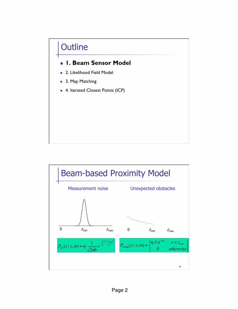
Beam-based Proximity Model
Measurement noise
zexp zmax 0
bzz
hit eb
mxzP2
exp )(21
21),|(
−−
=π
η⎭⎬⎫
⎩⎨⎧ <
=−
otherwisezz
mxzPz
0e
),|( expunexp
λλη
Unexpected obstacles
zexp zmax 0
Page 3!
5
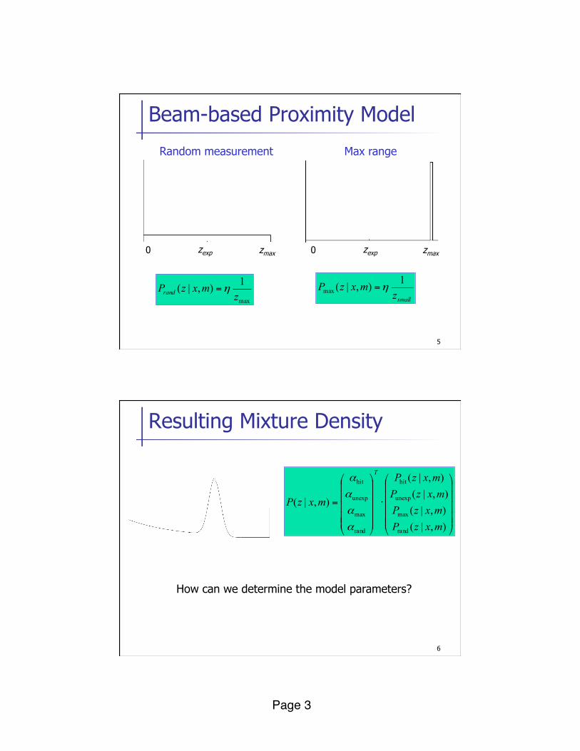
Beam-based Proximity Model
Random measurement Max range
max
1),|(z
mxzPrand η=smallz
mxzP 1),|(max η=
zexp zmax 0 zexp zmax 0
6
Resulting Mixture Density
⎟⎟⎟⎟⎟
⎠
⎞
⎜⎜⎜⎜⎜
⎝
⎛
⋅
⎟⎟⎟⎟⎟
⎠
⎞
⎜⎜⎜⎜⎜
⎝
⎛
=
),|(),|(),|(),|(
),|(
rand
max
unexp
hit
rand
max
unexp
hit
mxzPmxzPmxzPmxzP
mxzP
T
α
α
α
α
How can we determine the model parameters?
Page 4!
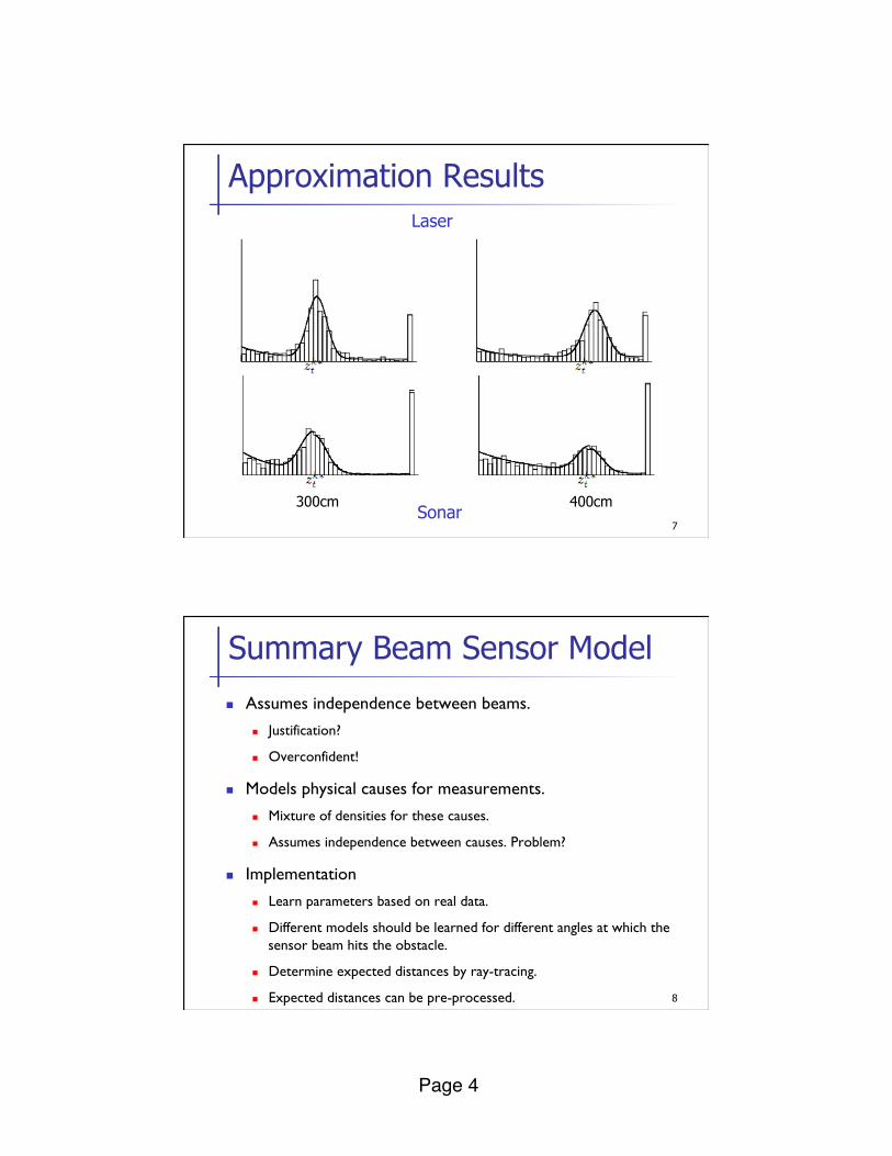
7
Approximation Results
Sonar
Laser
300cm 400cm
8
Summary Beam Sensor Model
n Assumes independence between beams. n Justification?
n Overconfident!
n Models physical causes for measurements.
n Mixture of densities for these causes.
n Assumes independence between causes. Problem?
n Implementation n Learn parameters based on real data.
n Different models should be learned for different angles at which the sensor beam hits the obstacle.
n Determine expected distances by ray-tracing.
n Expected distances can be pre-processed.
Page 5!
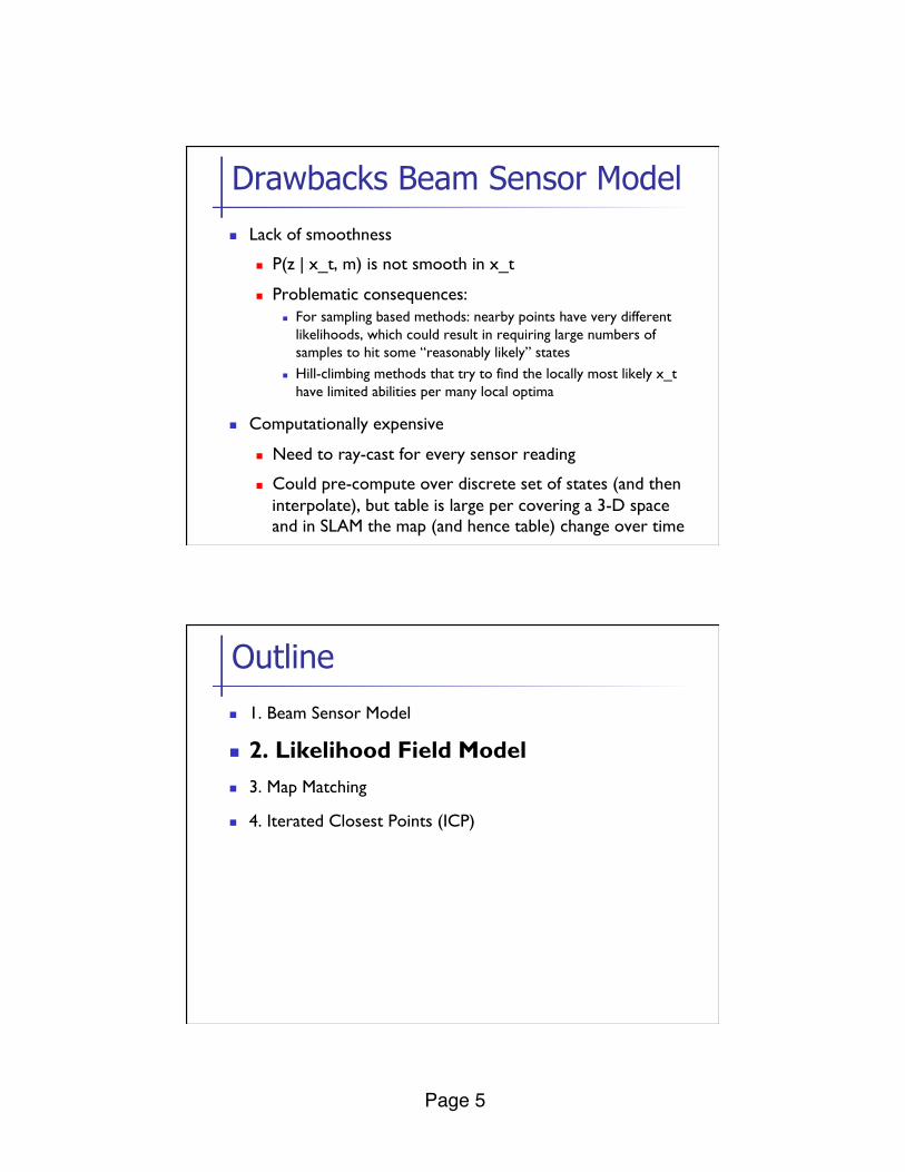
n Lack of smoothness
n P(z | x_t, m) is not smooth in x_t
n Problematic consequences: n For sampling based methods: nearby points have very different
likelihoods, which could result in requiring large numbers of samples to hit some “reasonably likely” states
n Hill-climbing methods that try to find the locally most likely x_t have limited abilities per many local optima
n Computationally expensive
n Need to ray-cast for every sensor reading
n Could pre-compute over discrete set of states (and then interpolate), but table is large per covering a 3-D space and in SLAM the map (and hence table) change over time
Drawbacks Beam Sensor Model
n 1. Beam Sensor Model
n 2. Likelihood Field Model n 3. Map Matching
n 4. Iterated Closest Points (ICP)
Outline
Page 6!
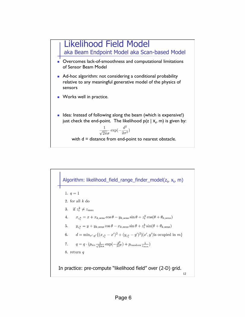
n Overcomes lack-of-smoothness and computational limitations of Sensor Beam Model
n Ad-hoc algorithm: not considering a conditional probability relative to any meaningful generative model of the physics of sensors
n Works well in practice.
n Idea: Instead of following along the beam (which is expensive!) just check the end-point. The likelihood p(z | xt, m) is given by:
with d = distance from end-point to nearest obstacle.
Likelihood Field Model aka Beam Endpoint Model aka Scan-based Model
12
Algorithm: likelihood_field_range_finder_model(zt, xt, m)
In practice: pre-compute “likelihood field” over (2-D) grid.
Page 7!
13
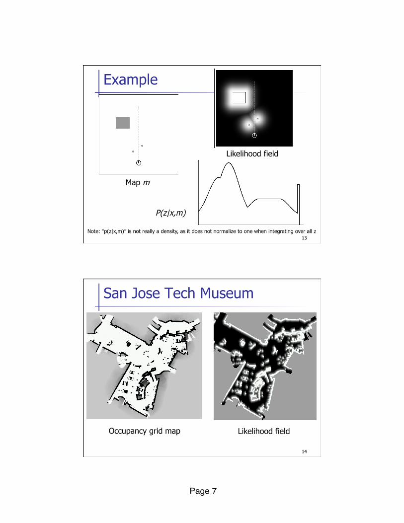
Example
P(z|x,m)
Map m
Likelihood field
Note: “p(z|x,m)” is not really a density, as it does not normalize to one when integrating over all z
14
San Jose Tech Museum
Occupancy grid map Likelihood field
Page 8!
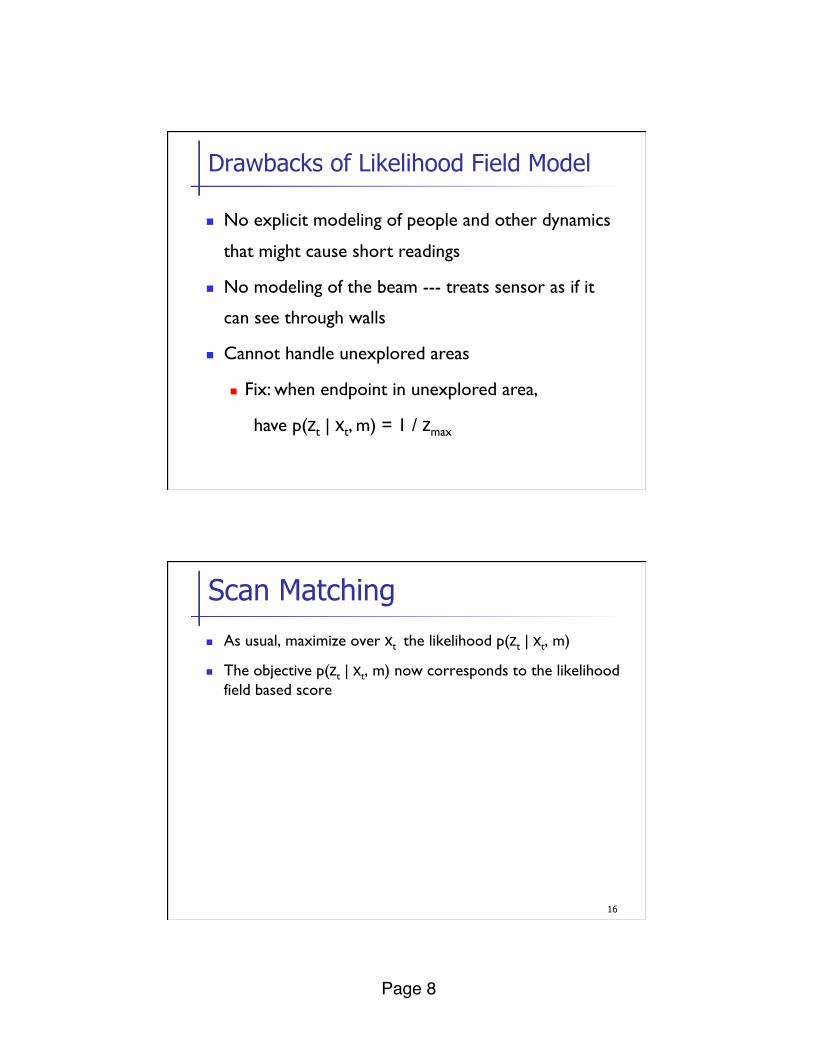
Drawbacks of Likelihood Field Model
n No explicit modeling of people and other dynamics
that might cause short readings
n No modeling of the beam --- treats sensor as if it
can see through walls
n Cannot handle unexplored areas
n Fix: when endpoint in unexplored area,
have p(zt | xt, m) = 1 / zmax
16
Scan Matching
n As usual, maximize over xt the likelihood p(zt | xt, m)
n The objective p(zt | xt, m) now corresponds to the likelihood field based score

Page 9!
17
Scan Matching
n Can also match two scans: for first scan extract likelihood field (treating each beam endpoint as occupied space) and use it to match the next scan. [can also symmetrize this]
18
Scan Matching
n Extract likelihood field from first scan and use it to match second scan.
~0.01 sec
Page 10!
19
Properties of Scan-based Model
n Highly efficient, uses 2D tables only.
n Smooth w.r.t. to small changes in robot position.
n Allows gradient descent, scan matching.
n Ignores physical properties of beams.
n 1. Beam Sensor Model
n 2. Likelihood Field Model
n 3. Map Matching n 4. Iterated Closest Points (ICP)
Outline
Page 11!
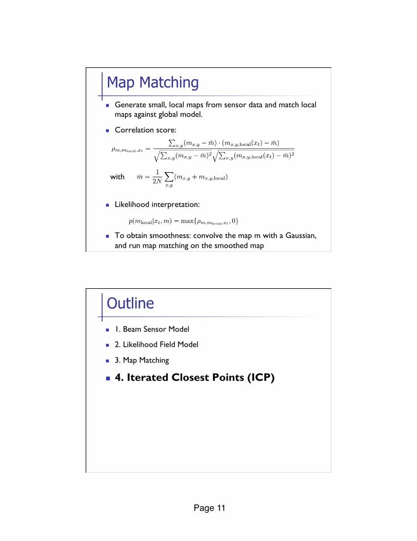
n Generate small, local maps from sensor data and match local maps against global model.
n Correlation score:
with
n Likelihood interpretation:
n To obtain smoothness: convolve the map m with a Gaussian, and run map matching on the smoothed map
Map Matching
n 1. Beam Sensor Model
n 2. Likelihood Field Model
n 3. Map Matching
n 4. Iterated Closest Points (ICP)
Outline
Page 12!
23
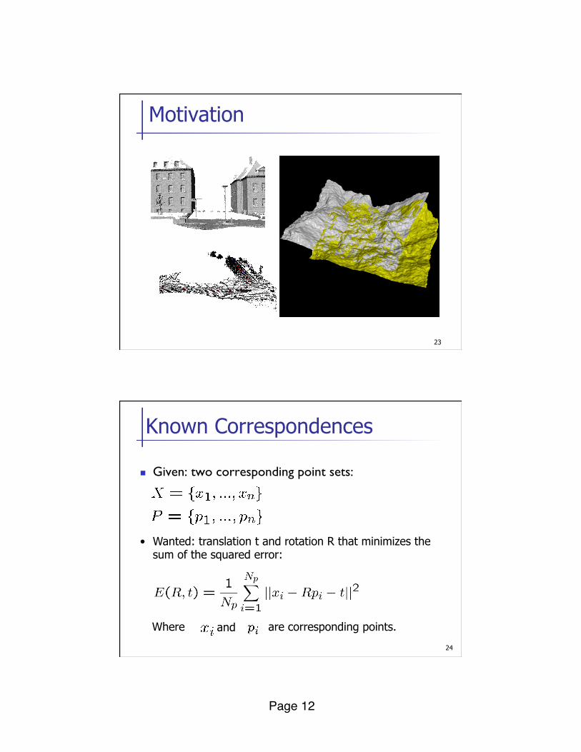
Motivation
24
Known Correspondences
n Given: two corresponding point sets:
• Wanted: translation t and rotation R that minimizes the sum of the squared error:
Where
are corresponding points. and
Page 13!
25
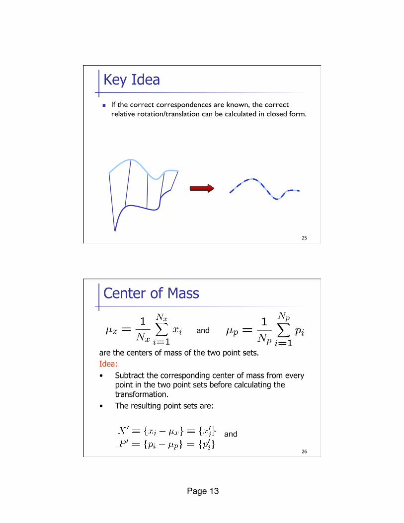
Key Idea
n If the correct correspondences are known, the correct relative rotation/translation can be calculated in closed form.
26
Center of Mass
and
are the centers of mass of the two point sets. Idea: • Subtract the corresponding center of mass from every
point in the two point sets before calculating the transformation.
• The resulting point sets are:
and
Page 14!
27
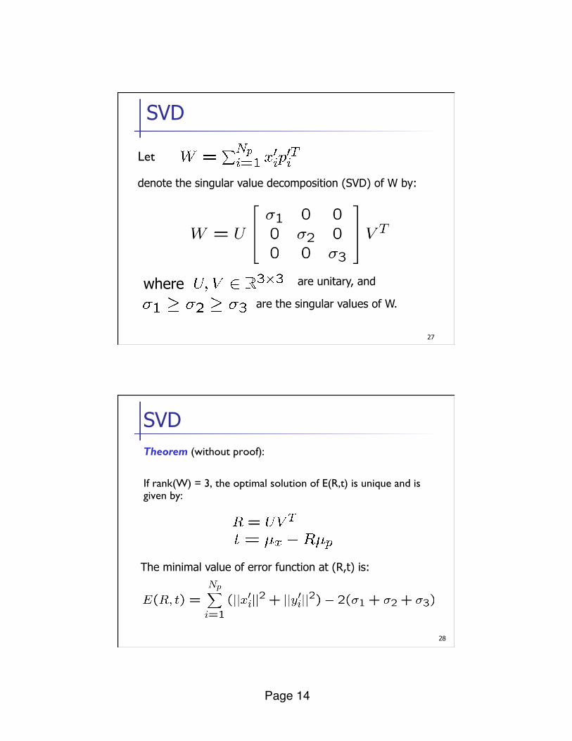
SVD
Let
denote the singular value decomposition (SVD) of W by:
where are unitary, and
are the singular values of W.
28
SVD Theorem (without proof): If rank(W) = 3, the optimal solution of E(R,t) is unique and is given by:
The minimal value of error function at (R,t) is:
Page 15!
29
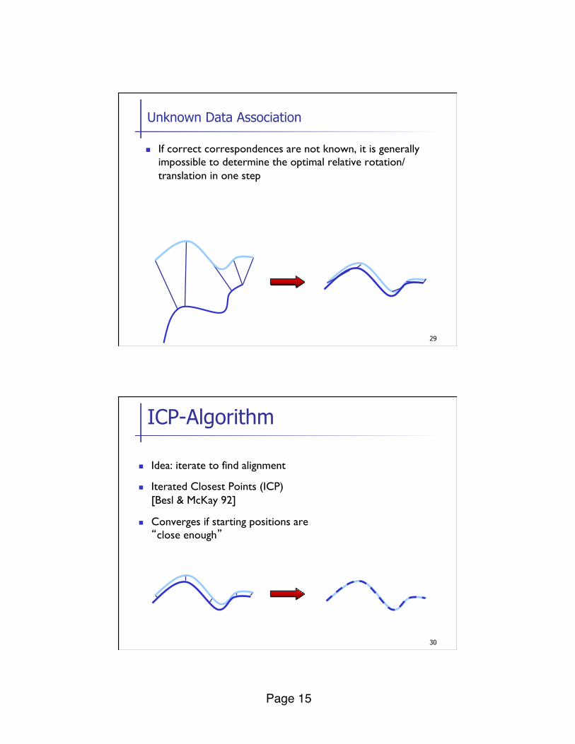
Unknown Data Association
n If correct correspondences are not known, it is generally impossible to determine the optimal relative rotation/translation in one step
30
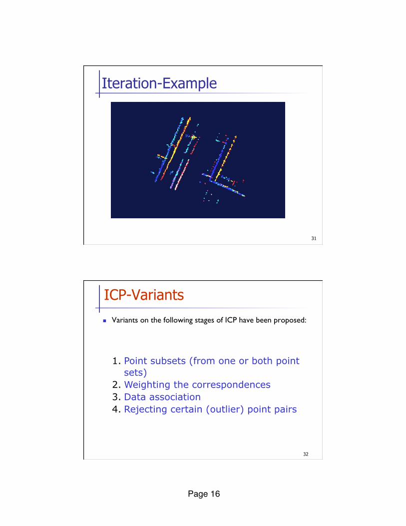
ICP-Algorithm
n Idea: iterate to find alignment
n Iterated Closest Points (ICP) [Besl & McKay 92]
n Converges if starting positions are “close enough”
Page 16!
31
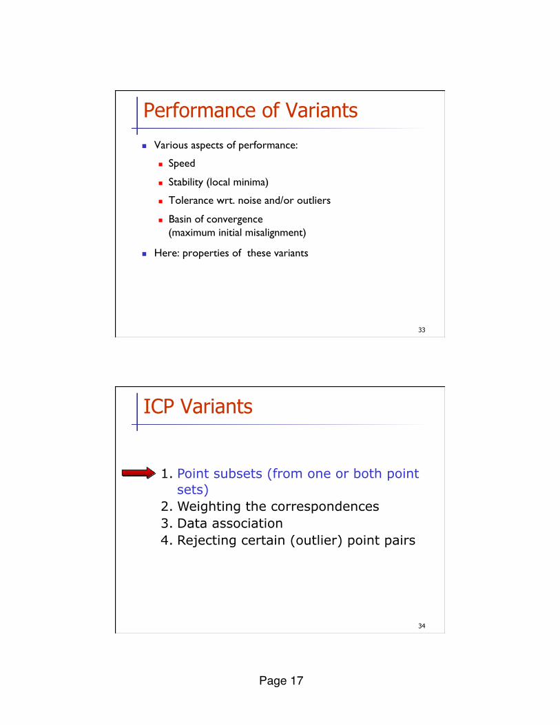
Iteration-Example
32
ICP-Variants
n Variants on the following stages of ICP have been proposed:
1. Point subsets (from one or both point sets)
2. Weighting the correspondences 3. Data association 4. Rejecting certain (outlier) point pairs
Page 17!
33
Performance of Variants
n Various aspects of performance:
n Speed
n Stability (local minima)
n Tolerance wrt. noise and/or outliers
n Basin of convergence (maximum initial misalignment)
n Here: properties of these variants
34
ICP Variants
1. Point subsets (from one or both point sets)
2. Weighting the correspondences 3. Data association 4. Rejecting certain (outlier) point pairs
Page 18!
35
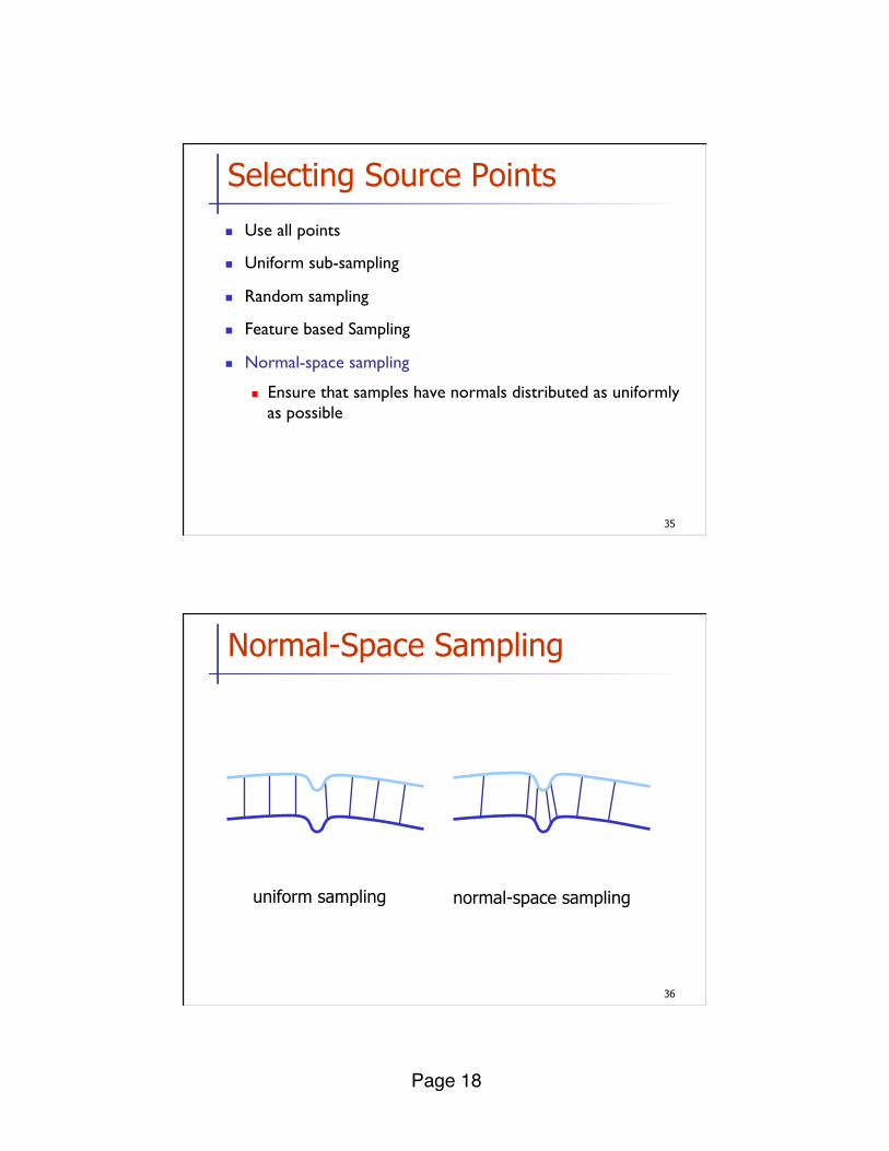
Selecting Source Points
n Use all points
n Uniform sub-sampling
n Random sampling
n Feature based Sampling
n Normal-space sampling
n Ensure that samples have normals distributed as uniformly as possible
36
Normal-Space Sampling
uniform sampling normal-space sampling
Page 19!
37
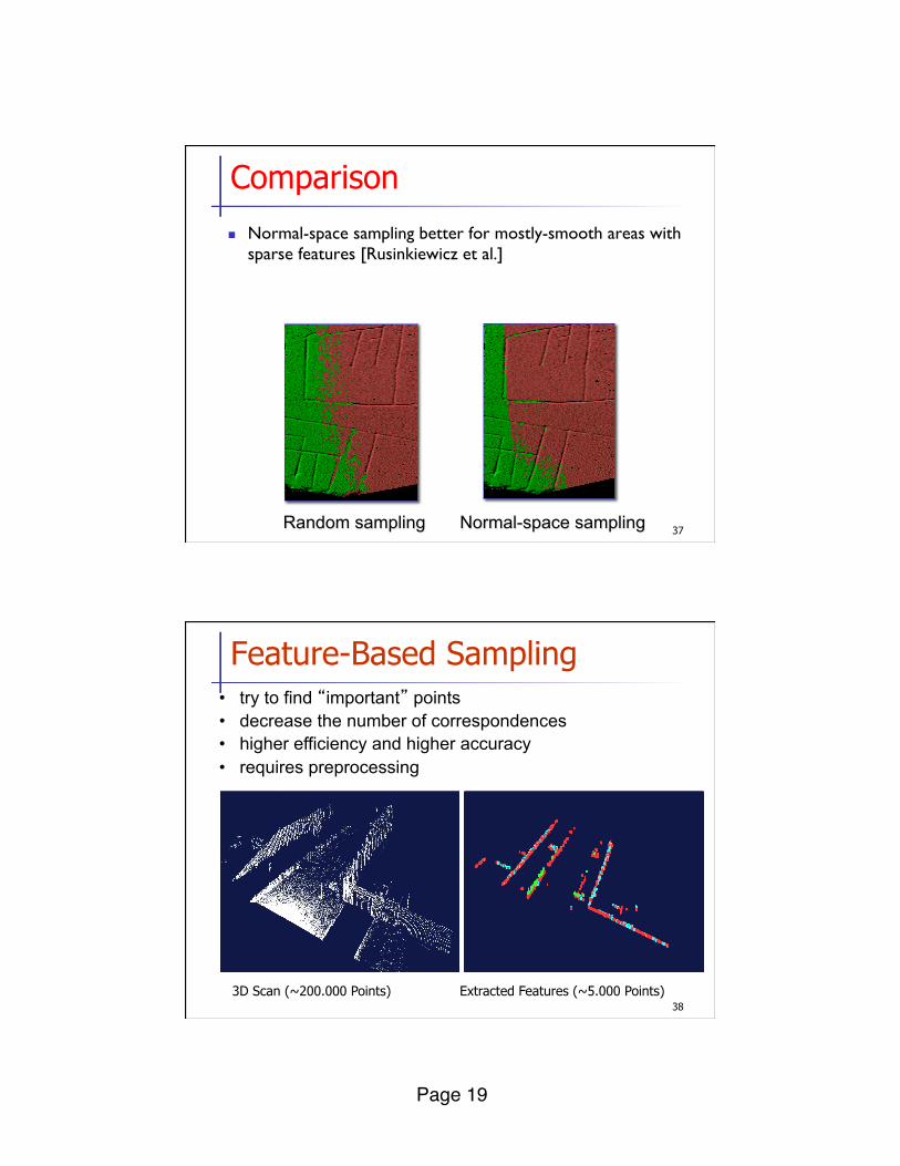
Comparison
n Normal-space sampling better for mostly-smooth areas with sparse features [Rusinkiewicz et al.]
Random sampling Normal-space sampling
38
Feature-Based Sampling
3D Scan (~200.000 Points) Extracted Features (~5.000 Points)
• try to find “important” points • decrease the number of correspondences • higher efficiency and higher accuracy • requires preprocessing
Page 20!
39
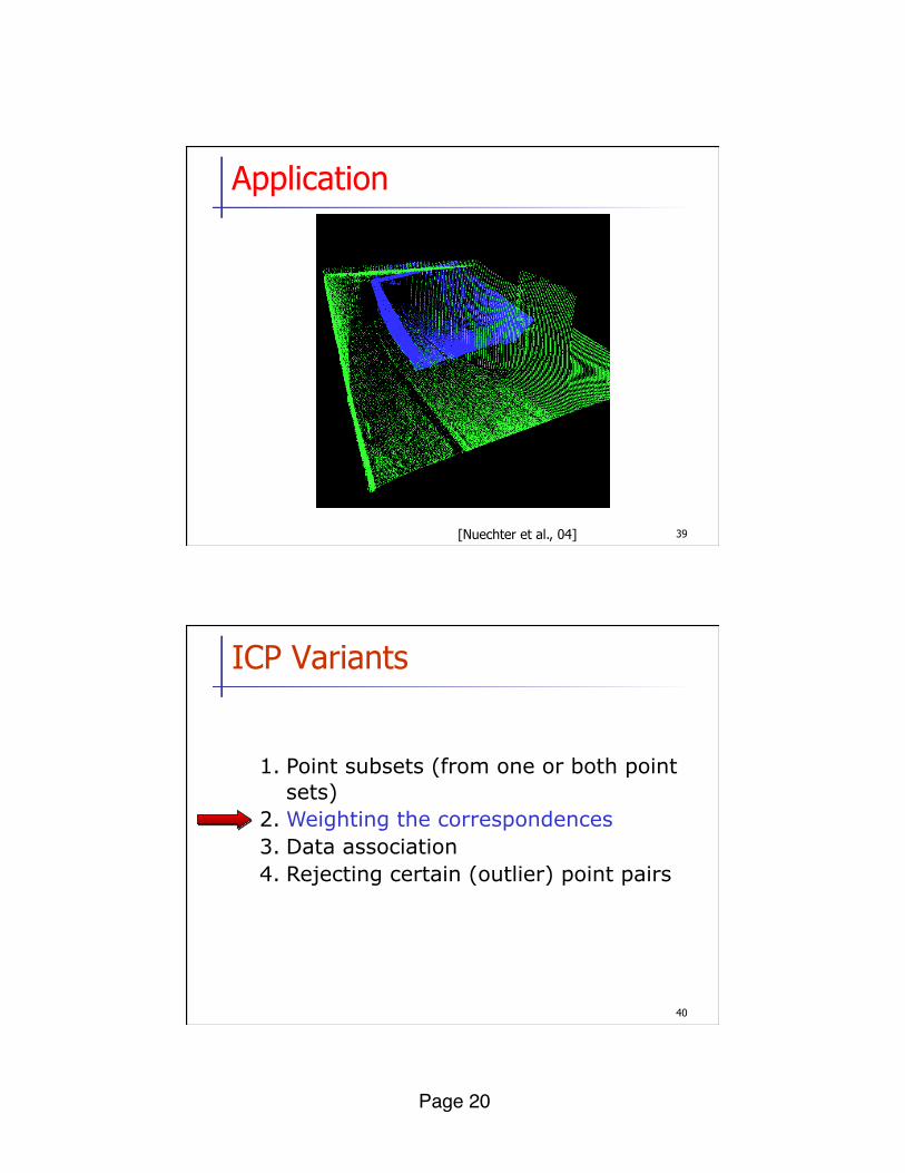
Application
[Nuechter et al., 04]
40
ICP Variants
1. Point subsets (from one or both point sets)
2. Weighting the correspondences 3. Data association 4. Rejecting certain (outlier) point pairs

Page 21!
41
Selection vs. Weighting
n Could achieve same effect with weighting
n Hard to guarantee that enough samples of important features except at high sampling rates
n Weighting strategies turned out to be dependent on the data.
n Preprocessing / run-time cost tradeoff (how to find the correct weights?)
42
ICP Variants
1. Point subsets (from one or both point sets)
2. Weighting the correspondences 3. Data association 4. Rejecting certain (outlier) point pairs
Page 22!
43
Data Association
n has greatest effect on convergence and speed
n Closest point
n Normal shooting
n Closest compatible point
n Projection
n Using kd-trees or oc-trees
44
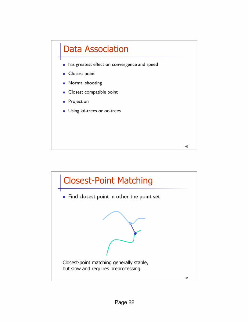
Closest-Point Matching
n Find closest point in other the point set
Closest-point matching generally stable, but slow and requires preprocessing
Page 23!
45
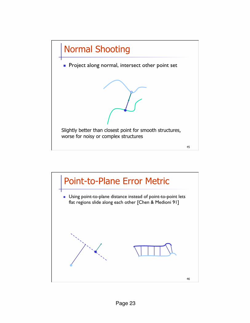
Normal Shooting
n Project along normal, intersect other point set
Slightly better than closest point for smooth structures, worse for noisy or complex structures
46
Point-to-Plane Error Metric
n Using point-to-plane distance instead of point-to-point lets flat regions slide along each other [Chen & Medioni 91]
Page 24!
47
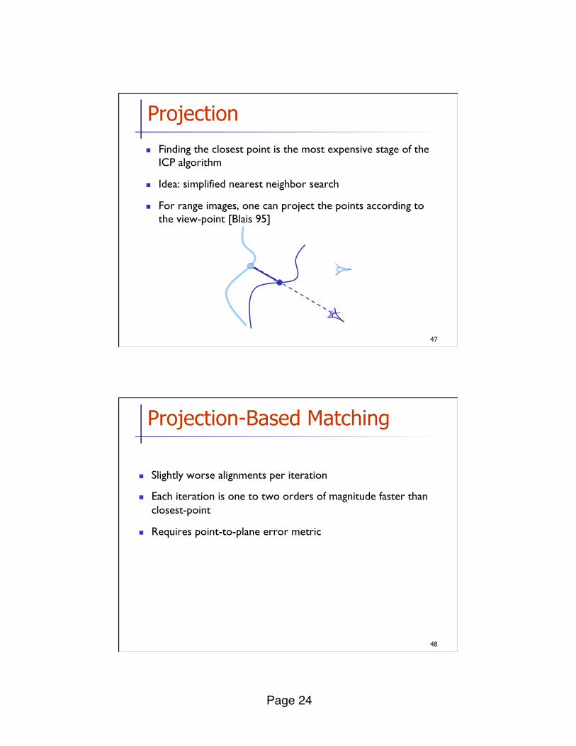
Projection
n Finding the closest point is the most expensive stage of the ICP algorithm
n Idea: simplified nearest neighbor search
n For range images, one can project the points according to the view-point [Blais 95]
48
Projection-Based Matching
n Slightly worse alignments per iteration
n Each iteration is one to two orders of magnitude faster than closest-point
n Requires point-to-plane error metric

Page 25!
49
Closest Compatible Point
n Improves the previous two variants by considering the compatibility of the points
n Compatibility can be based on normals, colors, etc.
n In the limit, degenerates to feature matching
50
ICP Variants
1. Point subsets (from one or both point sets)
2. Weighting the correspondences 3. Nearest neighbor search 4. Rejecting certain (outlier) point pairs
Page 26!
51
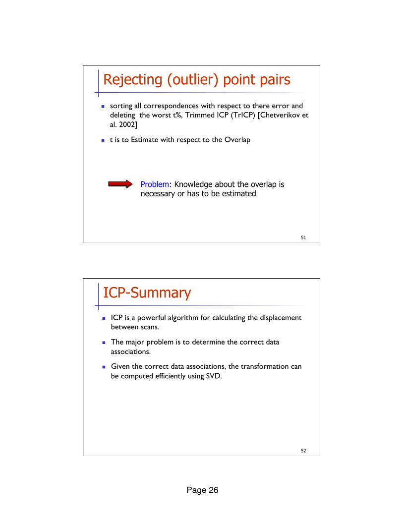
Rejecting (outlier) point pairs
n sorting all correspondences with respect to there error and deleting the worst t%, Trimmed ICP (TrICP) [Chetverikov et al. 2002]
n t is to Estimate with respect to the Overlap
Problem: Knowledge about the overlap is necessary or has to be estimated
52
ICP-Summary
n ICP is a powerful algorithm for calculating the displacement between scans.
n The major problem is to determine the correct data associations.
n Given the correct data associations, the transformation can be computed efficiently using SVD.