Scalar Network Analysis with U2000 Series USB … Network Analysis with U2000 Series USB Power Sensors Application Note Overview The Agilent U2000 Series USB power sensor is a compact,

Scalar Network Analysis with U2000 Series USB Power Sensors

Application Note

Overview The Agilent U2000 Series USB power sensor is a compact, light weight instru-

ment that performs accurate RF and microwave power measurements. Used with

a power splitter, coupler, and signal source, the U2000 provides scalar network

analysis (SNA) capability. This SNA capability allows you to perform stimulus-

response measurements such as gain, insertion loss, frequency response, and

return loss. These measurements are made to characterize the transmission or

reflection coefficient of devices such as cables, filters, amplifiers, and complex

systems encompassing multiple components, devices, and cables.

Some examples of stimulus-response measurements are:

• 3 dB bandwidth of a bandpass filter

• gain and return loss of an amplifier

• return loss of an antenna

• flatness of a low pass filter

• frequency response of a cable

Stimulus-response measurements require a source to stimulate the device

under test (DUT) and a receiver (in this case, a power sensor) to analyze the

DUT’s frequency response characteristics. While other Agilent power meters

and sensors may also be used for operations above 26.5 GHz, for simplicity, this

application note only focuses on the use of USB sensors.

This application note shows how to make accurate stimulus-response measure-

ments using:

• U2000 Series USB power sensors

• ESG/MXG/PSG signal generators

• broadband couplers

• power splitters

This application note also highlights the features of the U2000 Series for SNA

and compares its functionality with other test alternatives. It illustrates how the

U2000 Series addresses transmission, reflection, simultaneous transmission and

refection, and power sweep measurements. The uncertainties of transmission

and reflection measurement are also discussed.

2

Overview .................................................................................................... 1Comparing Test Equipment .................................................................... 3Transmission Measurements ................................................................ 6Transmission Measurement Uncertainties ....................................... 10Reflection Measurements .................................................................... 14Reflection Measurement Uncertainty ................................................ 17Simultaneous Transmission and Reflection Measurements ......... 22Transmission and Reflection Measurement Uncertainty ............... 25Power Sweep Measurement ............................................................... 26Optimizing Measurement Speed ......................................................... 27Summary ................................................................................................. 28Ordering Information ............................................................................. 29References .............................................................................................. 31Related Agilent Literature .................................................................... 31Appendix .................................................................................................. 32Agilent Advantage Services ..................................................Back coverContact Agilent .......................................................................Back cover

Table of Contents

3

Comparing Test Equipment

There are many test instruments capable of performing stimulus-response mea-

surements, including a USB sensor based scalar measurement setup, network

analyzers, and spectrum analyzers with tracking generators.

Network analyzers There are two types of network analyzers: vector or scalar. If phase information

is required, a vector network analyzer (VNA) is required. A VNA makes the most

accurate stimulus-response measurements by using vector error correction

algorithms. Swept tuned spectrum analyzers, scalar network analyzers (SNA),

and power meters are scalar instruments. Scalar network analyzers (like the dis-

continued Agilent 8757D) are the most popular instrument for measuring scalar

stimulus-response. Features offered by the scalar network analyzer include:

• Wide frequency coverage from 10 MHz to 110 GHz (detector dependent)

• Fast sweep time of 40 to 400 ms per sweep

• Multiple input ports for making simultaneous transmission and reflection

measurements without having to reconfigure or recalibrate the measurement

setup

• Flexible display formats, selectable from the front panel and calculated

inside the scalar network analyzer to allow visual analysis of the measured

transmission and reflection parameters

USB sensor based SNAs Comparatively, a USB sensor based SNA also has some attractive features.

The USB sensor based SNA offers a wide power range of –60 to +44 dBm

depending on the selected power sensor. It provides superior accuracy due to

its fully calibrated sensor, which provides an absolute measurement accuracy

of 3%. The frequency response uncertainty is minimized to within ±0.1 dB and

the calibration factor correction is stored inside the sensor’s memory. Perhaps

the most important feature is its dual use; apart from performing accurate power

measurements, USB sensors can also be setup to perform accurate scalar

power measurements with low overall setup cost.

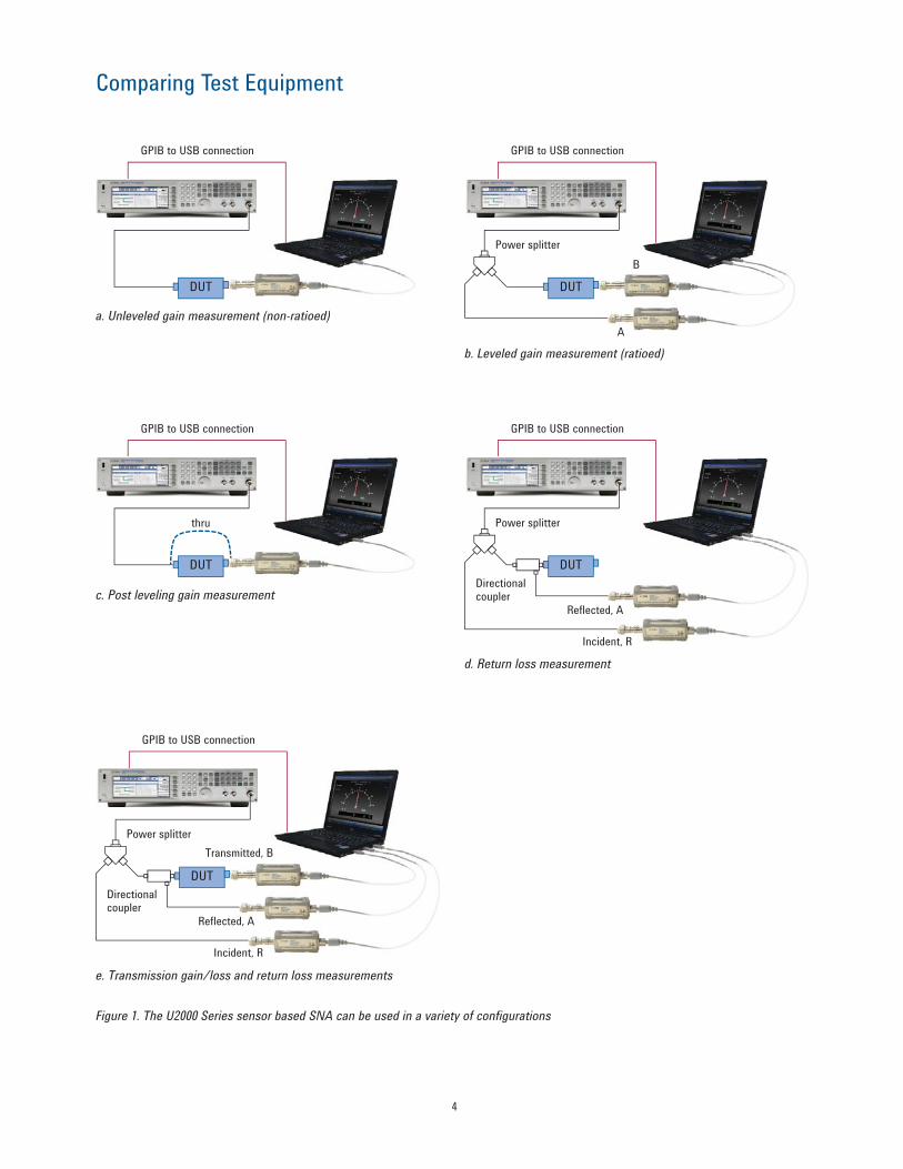
When U2000 Series USB sensors are used together with a signal source, power

splitter, and coupler, they can be transformed into a SNA to perform transmis-

sion gain or loss, and return loss measurements. Figure 1 shows a few different

configurations of a U2000 Series sensor based SNA. Free demonstration soft-

ware is available for download from Agilent’s Web site for each of the setups

shown in this application note. The demonstration software is compatible with

all Agilent EPM, EPM-P, P-Series power meters, and USB sensors.

www.agilent.com/find/SNAsoftware_download

4


Figure 1. The U2000 Series sensor based SNA can be used in a variety of configurations

e. Transmission gain/loss and return loss measurements

GPIB to USB connection

Incident, R

Reflected, A

Transmitted, B

Directional coupler

Power splitter

DUT

a. Unleveled gain measurement (non-ratioed)


DUT


A

B

Power splitter

DUT

b. Leveled gain measurement (ratioed)

d. Return loss measurement


Incident, R

Reflected, A

Directional coupler

Power splitter

DUT


DUT

thru

c. Post leveling gain measurement

5


Prior to performing actual SNA measurements using a U2000 Series device,

calibration is required in order to adjust the losses and mismatches due to the

power splitter, coupler, cables and adapters. The following section discusses

transmission power measurements and what calibrations are required.

Table 1 provides an overview comparing the different type of instrument capable

of performing scalar network analysis, including the discontinued Agilent 8757D

SNA and the next-generation U2000 series USB sensor based SNA.

Table 1. Test equipment options for stimulus-response measurements

8757D, detector and 85027x directional bridge

U2000 Series sensor based SNA

Dynamic range –60 to +16 dBm –60 to +20 dBm (U2000A)

–50 to +30 dBm (U2000H)

–30 to +44 dBm (U2000B)

Frequency range 10 MHz to 110 GHz (detector-dependent) 9 kHz to 26.5 GHz (sensor dependent)

(Frequency range up to 110 GHz is

available with Agilent power meter and

sensor combinations. Refer to ‘Ordering

Information’ section for millimeter wave

sensors)

Linearity Not specified 3%

Directivity 40 dB to 20 GHz

36 dB to 26.5 GHz

30 dB to 40 GHz

25 dB to 50 GHz

(bridge-dependent)

Coupler/bridge dependent

Example: 86205A bridge

40 dB to 2 GHz

30 dB to 3 GHz

20 dB to 5 GHz

16 dB to 6 GHz

Transmission measurement accuracy ~0.5 to 2.3 dB1

(dynamic accuracy + mismatch uncertainty)

~0.3 to 0.5 dB

(mismatch uncertainty + linearity)

Reflection measurement accuracy Mainly depend on the directivity of the

coupler/bridge

Mainly depend on the directivity of the

coupler/bridge

Return loss of detector/sensor (typical) at

2 GHz

18 GHz

20 dB

20 dB

40 dB

26 dB

Frequency response uncertainty to 18 GHz ±0.35 dB for precision detector

(up to ±2 dB for other detectors)

±0.1 dB

Measurement speed 40 to 400 ms per sweep

(75 ms for 2 traces with 201 points)

~50 ms per reading

(~10 second per sweep for 201 points)2

Price 8757D (discontinued): $21,000

Detector: $1,800 to $2,600

Total solution (18 GHz):

~$67,000 (including source)

~$35,000 (excluding source)

Total solution (18 GHz):

~$40,000 (including source)

~$14,000 (excluding source)

1. Extract from 8757D data sheet (literature number 5091-2471E).

2. Speed down to 15 ms per reading is available with Agilent P-Series power meters and sensors with external triggering sweep measurement

capability. For details, please refer to “Optimizing Measurement Speed” section.

6

Transmission Measurements

What are transmission measurements?

A scalar transmission measurement determines the gain or loss of a DUT. Let’s

take a look at some of the commonly used terms for transmission measurements.

EIncident

EReflected

DUT

ETransmitted

Figure 2. Common terms used in scalar network measurements

Terms used to define the transmission coefficient include:

Transmission coefficient (linear):

=

ETransmitted

EIncident

Transmission gain/loss (dB) = 20 log (gain)

= −20 log (loss)

= 20 log (ETransmitted

) – 20 log (EIncident

)

The transmission coefficient, , is equal to the transmitted voltage, ETransmitted

,

divided by the incident voltage, EIncident

. Since many displays are logarithmic,

transmission coefficient needs to be displayed in dB. This coefficient can be

applied to different transmission measurements. Attenuation, insertion loss, and

gain measurements can be expressed as follows:

Attenuation or Insertion loss (dB) = Pincident

(dBm) – Ptransmitted

(dBm)

Gain (dB) = Ptransmitted

(dBm) – Pincident

(dBm)

Where

Pincident

is incident power

Ptransmitted

is transmitted power

7


Making transmission measurement with U2000 Series sensor based SNA

There are a few methods of measuring transmission using the U2000 Series

sensor based SNA:

1. Unleveled transmission measurement

2. Leveled transmission measurement

3. Post leveling transmission measurement

Unleveled transmission measurement

Leveled transmission measurement Leveled transmission measurement uses a power splitter to split the source

power between the DUT and Sensor A (Figure 4). With the equal tracking

characteristic of a power splitter, the input power of the DUT is equal to the

measured power of Sensor A. Thus the transmission coefficient can be calcu-

lated as:

(Sensor_B_power) – (Sensor_A_power)

As its name implies, unleveled transmission measurements assume the output

power from the signal source is accurate and that there is minimum cable loss

from the source to the DUT (Figure 3). Thus the transmission coefficient can be

calculated as:

Sensor measured power – Signal source output power

Figure 3. Unleveled transmission measurement


DUT


A

B

Power splitter

DUT

Figure 4. Leveled transmission measurement

8


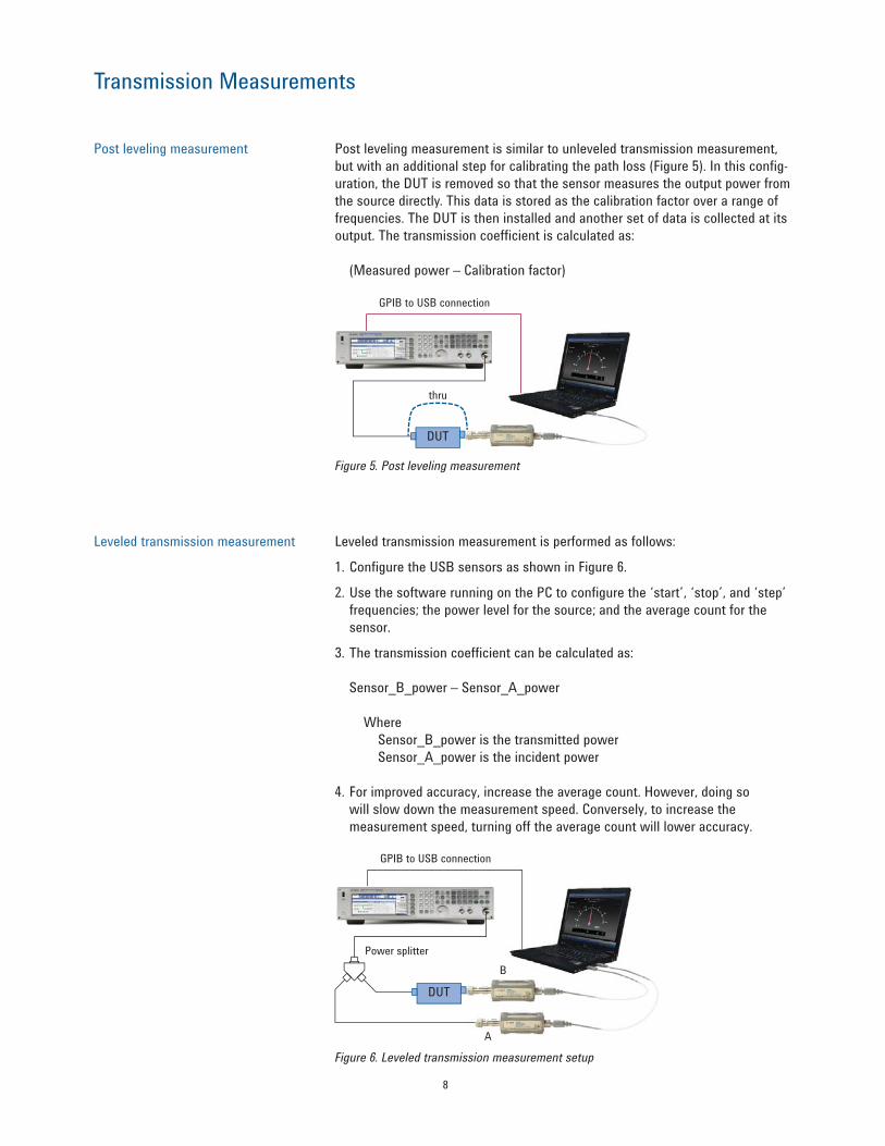
Post leveling measurement Post leveling measurement is similar to unleveled transmission measurement,

but with an additional step for calibrating the path loss (Figure 5). In this config-

uration, the DUT is removed so that the sensor measures the output power from

the source directly. This data is stored as the calibration factor over a range of

frequencies. The DUT is then installed and another set of data is collected at its

output. The transmission coefficient is calculated as:

(Measured power – Calibration factor)

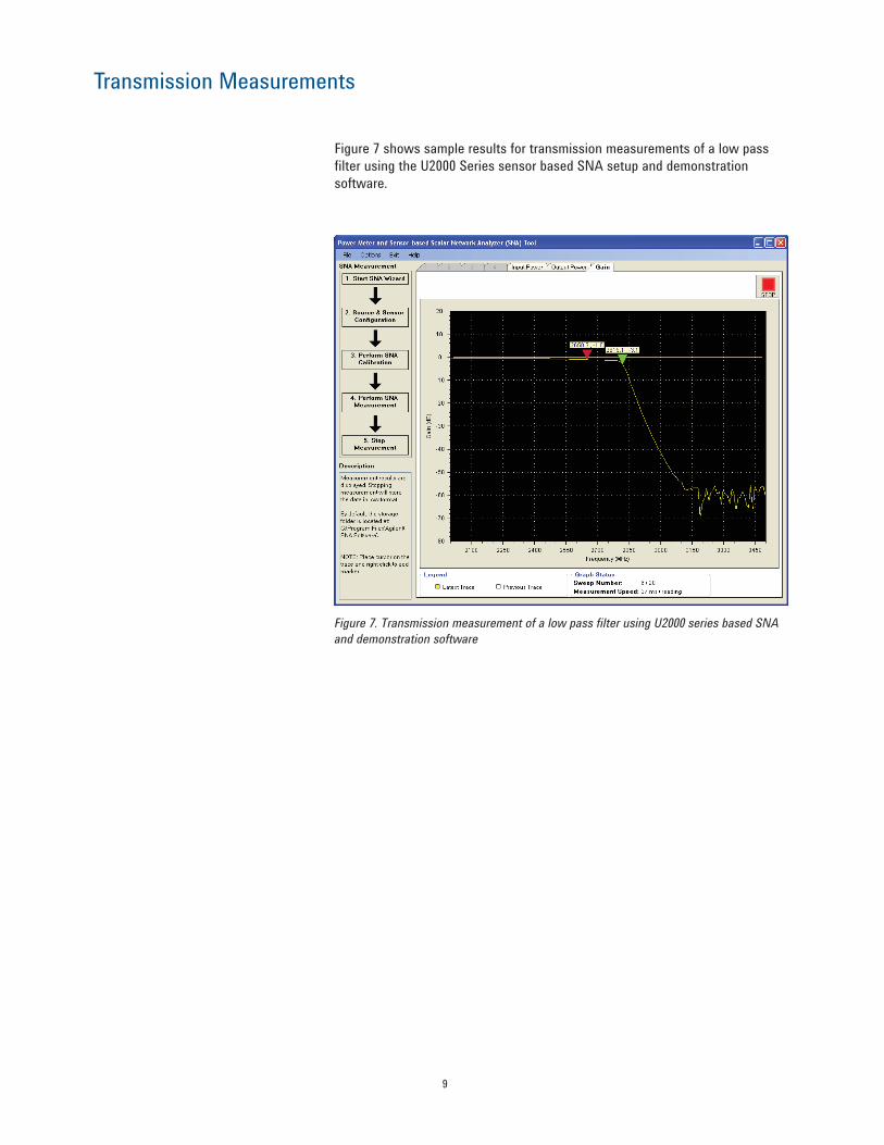
Leveled transmission measurement Leveled transmission measurement is performed as follows:

1. Configure the USB sensors as shown in Figure 6.

2. Use the software running on the PC to configure the ‘start’, ‘stop’, and ‘step’

frequencies; the power level for the source; and the average count for the

sensor.

3. The transmission coefficient can be calculated as:

Sensor_B_power – Sensor_A_power

Where

Sensor_B_power is the transmitted power

Sensor_A_power is the incident power

4. For improved accuracy, increase the average count. However, doing so

will slow down the measurement speed. Conversely, to increase the

measurement speed, turning off the average count will lower accuracy.


DUT

thru

Figure 5. Post leveling measurement


A

B

Power splitter

DUT

Figure 6. Leveled transmission measurement setup

9


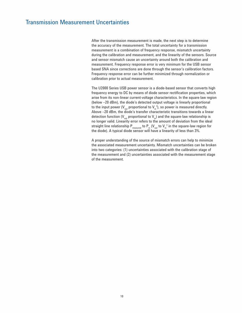
Figure 7 shows sample results for transmission measurements of a low pass

filter using the U2000 Series sensor based SNA setup and demonstration

software.

Figure 7. Transmission measurement of a low pass filter using U2000 series based SNA

and demonstration software

10

Transmission Measurement Uncertainties

After the transmission measurement is made, the next step is to determine

the accuracy of the measurement. The total uncertainty for a transmission

measurement is a combination of frequency response, mismatch uncertainty

during the calibration and measurement, and the linearity of the sensors. Source

and sensor mismatch cause an uncertainty around both the calibration and

measurement. Frequency response error is very minimum for the USB sensor

based SNA since corrections are done through the sensor’s calibration factors.

Frequency response error can be further minimized through normalization or

calibration prior to actual measurement.

The U2000 Series USB power sensor is a diode-based sensor that converts high

frequency energy to DC by means of diode sensor rectification properties, which

arise from its non-linear current-voltage characteristics. In the square-law region

(below –20 dBm), the diode’s detected output voltage is linearly proportional

to the input power (Vout

proportional to Vin

2), so power is measured directly.

Above –20 dBm, the diode’s transfer characteristic transitions towards a linear

detection function (Vout

proportional to Vin) and the square-law relationship is

no longer valid. Linearity error refers to the amount of deviation from the ideal

straight line relationship Pmeasured

to Pin (V

out to V

in2 in the square-law region for

the diode). A typical diode sensor will have a linearity of less than 3%.

A proper understanding of the source of mismatch errors can help to minimize

the associated measurement uncertainty. Mismatch uncertainties can be broken

into two categories: (1) uncertainties associated with the calibration stage of

the measurement and (2) uncertainties associated with the measurement stage

of the measurement.

11

Mismatch uncertainties for calibration

Mismatch uncertainties for calibration are due to the impedance mismatch

between the source and the sensor. A portion of the incident signal is reflected

back towards the source because of the sensor’s input match. This reflected

signal is then re-reflected by the source impedance mismatch, resulting in an

uncertainty vector related to the incident signal at some unknown phase. This

uncertainty vector can add or subtract from the actual measured amplitude,

causing an error in the calibration measurement.

For uncertainties associated with the calibration stage (Figure 8), when the sen-

sor is connected to the source, the incident signal first encounters the sensor

impedance, where part of the incident signal is reflected. This reflected signal

is then re-reflected by the source mismatch, resulting in an uncertainty vector

of ρs x ρ

d at some unknown phase relationship to the incident signal. The worst

case of the signal seen by the sensor would be 1 ± ρs x ρ

d.

Figure 8. Mismatch uncertainties for calibration (post leveling

transmission measurement)



1.4SWR

1.13SWR

EIncident

ρd

1 ± ρs ρ

d

ρs ρ

d

12


Mismatch uncertainties for measurement

Mismatch uncertainties during the measurement of the DUT are caused by the

source/device input mismatch and device output/sensor mismatch (Figure 9).

Uncertainties in the measurement stage are due to source/DUT input mismatch

(1 ± ρs x ρ

1) and DUT output/sensor mismatch (1 ± ρ

d x ρ

2).

Because the transmission coefficient of the device is the difference between the

calibration value and the measured value, the overall mismatch uncertainties

are a combination of the mismatch during calibration and measurement.

Figure 9. Mismatch uncertainties for measurement (post leveling

transmission measurement)

Calculating transmission measurement errors

To get a feel for the errors associated with transmission measurement, let’s cal-

culate typical worst case uncertainties based on the post leveling transmission

measurement previously described.

To calculate the mismatch errors, the standing wave ratio (SWR) needs to be

converted to the reflection coefficient, ρ.

ρ =

SWR – 1

SWR + 1

At 1 GHz, the MXG output SWR is 1.4 while the U2000A SWR is 1.13. Assuming

the DUT input and output SWR is 1.2, the reflection coefficient can be calcu-

lated as:

ρs = 0.167; ρ

d = 0.061; ρ

1 = 0.091; ρ

2 = 0.091


1.4SWR

1.13SWR

DUT

1.2 SWR

1.2 SWR

ρs

ρdρ

1ρ

2

EIncident

1 ± ρd ρ

2

ρs ρ

1ρ

d ρ

2

1 ± ρs ρ

1

13


The U2000A’s linearity is less than 3%. The worst case transmission measure-

ment uncertainty can be calculated as:

Transmission uncertainty = ±{[calibration mismatch uncertainties] +

[measurement mismatch uncertainties] +

[2 x linearity]}

Transmission uncertainty (dB) = [20 log(1 ± (ρs x ρ

d))] + [20 log(1 ± (ρ

s x ρ

1)) +

20 log(1 ± (ρd x ρ

2)) + 2 x 10 log (1 ± 3%)]

= 0.527 dB, –0.530 dB

This is the worst case uncertainty for transmission measurement of a USB

sensor based SNA. In this example, it is assumed that the DUT has an input-

to-output isolation of better than 3 dB so that multiple reflections have a

negligible effect on the uncertainty. For a low loss, bidirectional device, the

term “20 log (1 ± ρs x ρ

d)” will be part of the measurement uncertainties and

therefore will occur twice in the maximum mismatch error equation.

To further improve the transmission measurement uncertainties, the ratio tech-

nique can be used to improve the source match.

Source match can be improved by calculating the ratio of the incident and

reflected signals (Figure 6). With this technique, any variation in the incident

signal is being ratioed out. Any re-reflections are seen by both sensors and

when the ratio of transmission/reflected signal is obtained, the effect of source

match is cancelled. A power splitter is a good choice for ratio technique due to

its small size and broadband response. The source match in this case will be

replaced by the output match of the power splitter.

At 1 GHz, a power splitter output SWR is 1.10(ρs’= 0.0476). The transmission

measurement uncertainty can be improved to:

Transmission uncertainty (dB) = [20 log (1 ± ρs’ x ρ

d)] + [20 log (1 ± ρ

s’ x ρ

1) +

20 log (1 ± ρd x ρ

2) + 2 x 10 log (1 ± 3%)]

= 0.371 dB, –0.371 dB

With ratio technique, the transmission uncertainty has been improved from

around ±0.53 to ±0.37 dB. This is the worst case uncertainty for transmission

measurement.

An attenuation pad is frequently used to improve the mismatch between the

detector of SNA and DUT. The attenuator pad is used because of the poor input

match of the detector. U2000 Series USB power sensors have good input match

thus the addition of attenuation pad is typically not required.

14

Reflection Measurements

What are reflection measurements?

A scalar reflection measurement is concerned with how efficiently energy is

transferred to a DUT (Figure 10). It is a measure of the amount of mismatch

between a DUT and a Zo transmission line (Z

o = characteristic impedance,

typically 50 Ω). Not all the energy incident upon a device is absorbed by the

device, and the portion not absorbed is reflected back towards the source. The

efficiency of energy transfer can be determined by comparing the incident and

reflected signals.

The reflection coefficient, ρ, is equal to the ratio of reflected voltage wave,

EReflected

, to the incident voltage wave, EIncident

. For a transmission line of charac-

teristic impedance, Zo, terminated with a perfectly matched load, all the energy

is transferred to the load and none is reflected: EReflected

= 0 then ρ = 0. When the

same transmission line is terminated with an open or short circuit, all the energy

is reflected back: EReflected

= EIncident

then ρ = 1. Therefore, the possible values for

ρ are 0 to 1.

Reflection coefficient, ρ =

EReflection

EIncident

Since many displays are logarithmic, a term to express the reflected coefficient

in dB is needed. Return loss is the logarithmic expression of the relationship

between the reflected signal and the incident signal. Return loss can be

calculated as –20 log ρ. Thus the range of values for return loss is infinity (for a

matched load) to 0 (for an open or short circuit).

Return loss = –20 log ρ

Another term commonly used is standing-wave-ratio (SWR). Standing waves are

caused by the interaction of the incident and reflected waves along a transmis-

sion line. The SWR equals the maximum envelope voltage of the combined trav-

elling waves over the minimum envelope voltage. SWR can also be calculated

from the reflection coefficient: SWR = (1 + ρ)/(1 – ρ) and ranges from 1 (for a

matched load) to infinity (open or short circuit).

SWR =

1 + ρ

1 – ρ

Figure 11. Reflection measurement relationships between matched load and

open/short circuit

Match load Open/short

SWR1 Infinity

Return lossInfinity 0 dB

ρ0 1

EIncident

EReflected

DUT

ETransmitted

Figure 10. Overview of scalar reflection measurement concept

15


Directional coupler or bridge Before we discuss reflection measurements in detail, let’s try to understand

more about signal separation devices, such as a coupler or a bridge, which are

crucial for accurate reflection measurements (Figure 12 and Figure 13).

A directional coupler, or bridge, will couple a portion of the signal flowing

through the main arm to the auxiliary arm. The coupling factor is the relationship

between the coupled path, or the auxiliary arm, to the through-path or main arm,

expressed in dB. If the coupler is turned around and the signal is allowed to flow

in the reverse direction through the coupler, ideally there will be no power in the

auxiliary arm. However, some energy will leak through the coupler. A measure of

this leakage signal is defined as isolation of the coupler.

Another term frequently associated with couplers is directivity. Directivity is

the ability of the coupler to separate signals flowing in the opposite directions.

Directivity is defined as the ratio of power measured in the auxiliary arm with

a coupler connected in the forward direction, to the power measured in the

auxiliary arm with a coupler connected in the reverse direction. In both cases,

the coupler output will have to be terminated with a Zo load with the same input

power level being applied:

Directivity =

Coupling factor

Isolation

Directivity (in dB) = Isolation (dB) – Coupling factor (dB)

Where

Coupling factor (dB) = –10 log [P(coupling factor, forward direction)]

P(in)

Isolation (dB) = –10 log [P(coupling factor, reverse direction)]

P(in)

Linear term directivity = 10

–Directivity (dB)

20

The sources of imperfect directivity are leakages, internal coupler load reflec-

tions, and connector reflections.

In general, a broadband coupler has insertion loss in the order of 1 dB. On the

other hand, a directional bridge has insertion loss of at least 6 dB. This loss will

directly subtract from the dynamic range of the measurements.

Figure 12. Agilent 86205A and 86207A

directional bridge

Figure 13. Agilent 773D directional coupler

16


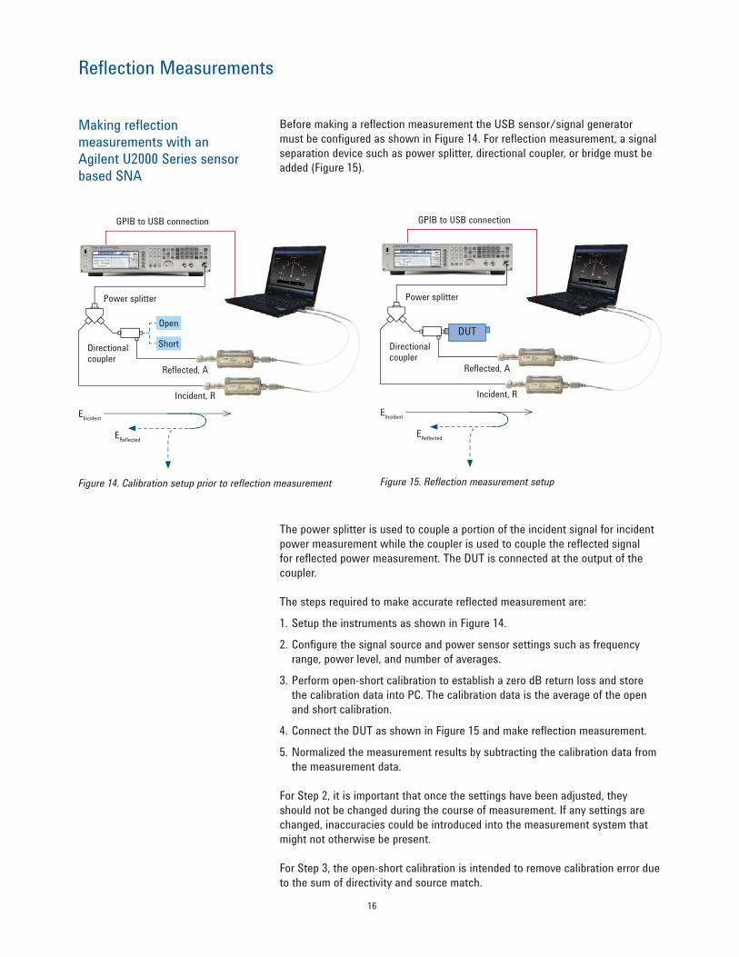
Making reflection measurements with an Agilent U2000 Series sensor based SNA

Before making a reflection measurement the USB sensor/signal generator

must be configured as shown in Figure 14. For reflection measurement, a signal

separation device such as power splitter, directional coupler, or bridge must be

added (Figure 15).

The power splitter is used to couple a portion of the incident signal for incident

power measurement while the coupler is used to couple the reflected signal

for reflected power measurement. The DUT is connected at the output of the

coupler.

The steps required to make accurate reflected measurement are:

1. Setup the instruments as shown in Figure 14.

2. Configure the signal source and power sensor settings such as frequency

range, power level, and number of averages.

3. Perform open-short calibration to establish a zero dB return loss and store

the calibration data into PC. The calibration data is the average of the open

and short calibration.

4. Connect the DUT as shown in Figure 15 and make reflection measurement.

5. Normalized the measurement results by subtracting the calibration data from

the measurement data.

For Step 2, it is important that once the settings have been adjusted, they

should not be changed during the course of measurement. If any settings are

changed, inaccuracies could be introduced into the measurement system that

might not otherwise be present.

For Step 3, the open-short calibration is intended to remove calibration error due

to the sum of directivity and source match.

Figure 14. Calibration setup prior to reflection measurement


Incident, R

Reflected, A

Directional coupler

Power splitter

EIncident

EReflected

Figure 15. Reflection measurement setup


Incident, R

Reflected, A

Directional coupler

Power splitter

DUT

EIncident

EReflected

Open

Short

17

Reflection Measurement Uncertainty

Now that the reflection measurement has been made, the accuracy of the mea-

surement must be determined. The measurement uncertainty associated with

reflection measurement is comprised of three terms:

∆ρ = A + Bρ + Cρ2

This equation is a simplification of a complex flow-graph analysis. ∆ρ is the

worst case uncertainty for the reflection measurement where ρ is the measured

reflection coefficient of the device. A, B, and C are linear terms and an explana-

tion of each term follows.

Term A: Directivity Directivity is the ability of the bridge or coupler to separate signals flowing in

opposite directions. Since no signal separation device is perfect, some of the

incident energy flowing in the main arm of the coupler may leak across the

auxiliary arm, causing an error in the signal level measured by the sensor. This

directivity signal is independent of the reflection coefficient of the DUT and

adds (worst case) directly to the total uncertainty. If the signal reflected from

the DUT is large, for example for a short circuit, then the directivity will be small

compared to the reflected signal. The effect of directivity will be insignificant. If

the signal reflected from the DUT is small (high return loss), then the directivity

signal will be significant compare to the reflected signal. Thus the uncertainty

due to directivity will be significant in this case (Figure 16). Therefore, the signal

separation device selected is extremely important to the accuracy of the reflec-

tion measurement. A recommended bridge is the Agilent 86205A which has

directivity of up to 40 dB. Since the impact of directivity cannot be removed, it is

important to select a separation device with high enough directivity.

Directivity error (dB) vs. reflection uncertainty

5

3

1

–1

–3

–5

Max

imum

err

or

(dB

)

0 10 20 30 40

DUT return loss (dB)

Directivity = 30

Directivity = 40

Directivity = 20

Figure 16. Effect of coupler directivity to the reflection

measurement uncertainty

18

Term B: Calibration error When calibrating the system with a standard (open or short), some error terms

will also be measured. Directivity and source match are the error terms that

always present and will be measured. If it is assume that no other errors are

present, then the best case calibration error (B) is equal to the sum of directivity

and source match:

B = A + C

Figure 17 shows the frequency response of a open standard. Notice the ripple

caused by source match and directivity error vectors. Another standard, short

circuit could also be used as a calibration standard. Notice that the ripple is still

present, but the phase is different (Figure 18). The calibration error due to the

sum of the directivity and source match errors can be removed by averaging the

short and open circuit responses. Though the reflection from an open circuit is

180 degrees out of phase compared to a short circuit, the errors due to the sum

of directivity and source match do not change phase when the load is changed

from an open to a short. Thus open/short average then averages out calibration

error thus making B = 0. Figure 18 shows the open/short average. Notice that

the ripples are removed.


Open/short average could be calculated as:

Open/short average =

Copen + C

short

2

Where

Copen

is the linear term reflection coefficient for an open standard

Cshort

is the linear term reflection coefficient for a short standard

Open/short average (in dB) = 20 log ( 10

–Copen(dB)

+ 10

–Cshort(dB)

) 20 20

2

Where

Copen(dB)

is the reflection coefficient in dB for an open standard

Cshort(dB)

is the reflection coefficient in dB for a short standard

18.4

18.2

18

17.8

17.6

17.4

17.2

17

50 200

350

500

650

800

950

1100

1250

1400

1550

Frequency (MHz)

Open

18.4

18.2

18

17.8

17.6

17.4

17.2

17

50 210

370

530

690

850

1010

1170

1330

1490

Frequency (MHz)

Open/short

average

Short

Open

Figure 17. Frequency response of a short standard Figure 18. Frequency response of a short standard (red) and

open/short average (green)

19


Term C: Effective source match A perfect source match would deliver a constant power to the load regardless

of the reflection from the load. If the source match is not perfect, signals will be

re-reflected, adding to the incident signal at some unknown phase, and causing

an error in the measurement. Figure 19 shows that the first reflection from the

DUT is ρL. This is the signal to measure (reflection coefficient of the DUT). This

signal flows towards the source, where it is re-reflected if the source match is

not perfect. This results in a signal ρLρ

S flowing back toward the DUT where it

is again re-reflected and sampled as ρL2ρ

S. When the reflected signal, ρ

L, is large

(low return loss), source match will cause a significant error. If ρL is small, then

the effect of source match is insignificant (Figure 20). Recall that this is directly

opposite with the effect of directivity, whereby directivity effect is significant for

high return loss and less significant for low return loss.

Source match error (dB) vs. reflection uncertainty

5

4

3

2

1

0

–1

–2

–3

–4

–5

Max

imum

err

or

(dB

)

0 10 20 30 40

DUT return loss (dB)

VSWR = 1.25

VSWR = 2.0

VSWR = 1.25

VSWR = 2.0

Figure 20. Effect of source match to the reflection measurement uncertainty

ρL ρ

S

Figure 19. Ratio measurement technique is used to improve source match


Incident, R

Reflected, A

Directional coupler

Power splitter

DUT

EIncident

ρL

ρL2 ρ

S

ρL2 ρ

S

ρL

20


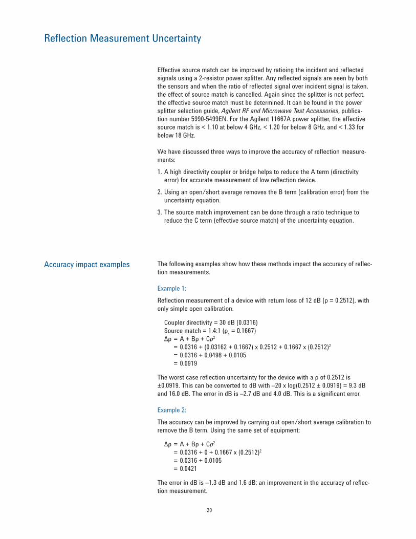
Effective source match can be improved by ratioing the incident and reflected

signals using a 2-resistor power splitter. Any reflected signals are seen by both

the sensors and when the ratio of reflected signal over incident signal is taken,

the effect of source match is cancelled. Again since the splitter is not perfect,

the effective source match must be determined. It can be found in the power

splitter selection guide, Agilent RF and Microwave Test Accessories, publica-

tion number 5990-5499EN. For the Agilent 11667A power splitter, the effective

source match is < 1.10 at below 4 GHz, < 1.20 for below 8 GHz, and < 1.33 for

below 18 GHz.

We have discussed three ways to improve the accuracy of reflection measure-

ments:

1. A high directivity coupler or bridge helps to reduce the A term (directivity

error) for accurate measurement of low reflection device.

2. Using an open/short average removes the B term (calibration error) from the

uncertainty equation.

3. The source match improvement can be done through a ratio technique to

reduce the C term (effective source match) of the uncertainty equation.

Accuracy impact examples The following examples show how these methods impact the accuracy of reflec-

tion measurements.

Example 1:

Reflection measurement of a device with return loss of 12 dB (ρ = 0.2512), with

only simple open calibration.

Coupler directivity = 30 dB (0.0316)

Source match = 1.4:1 (ρs = 0.1667)

∆ρ = A + Bρ + Cρ2

= 0.0316 + (0.03162 + 0.1667) x 0.2512 + 0.1667 x (0.2512)2

= 0.0316 + 0.0498 + 0.0105

= 0.0919

The worst case reflection uncertainty for the device with a ρ of 0.2512 is

±0.0919. This can be converted to dB with –20 x log(0.2512 ± 0.0919) = 9.3 dB

and 16.0 dB. The error in dB is –2.7 dB and 4.0 dB. This is a significant error.

Example 2:

The accuracy can be improved by carrying out open/short average calibration to

remove the B term. Using the same set of equipment:

∆ρ = A + Bρ + Cρ2

= 0.0316 + 0 + 0.1667 x (0.2512)2

= 0.0316 + 0.0105

= 0.0421

The error in dB is –1.3 dB and 1.6 dB; an improvement in the accuracy of reflec-

tion measurement.

21

Example 3:

Ratio technique with a power splitter can further improve the accuracy. Source

match can be improved from 1.4 to 1.10 with the use of power splitter:

∆ρ = A + Bρ + Cρ2

= 0.0316 + 0 + 0.0476 x (0.2512)2

= 0.0346

The error is now improved to –1.1 dB and 1.3 dB.

Example 4:

A good directivity coupler can be used to further improve the accuracy. Below is

the improvement for a coupler with 40 dB of directivity:

∆ρ = A + Bρ + Cρ2

= 0.01 + 0 + 0.0476 x (0.2512)2

= 0.013

The error is now improved to –0.44 dB and 0.46 dB, a significant improvement

compared to 4 dB of error in Example 1.

Steps for accurate reflection measurement

In summary, to make an accurate reflection measurement using USB sensor

based SNA, perform the following steps:

1. Setup the measurement using the ratio technique with power splitter and

directional coupler or bridge.

2. Choose a coupler or bridge with good directivity (e.g. Agilent 86205A.)

3. Setup the frequency range, power level, and average count.

4. Perform open/short average calibration. Do not change settings after

calibration.

5. Make measurement by connecting the DUT.


the measurement data.


22

Simultaneous Transmission and Reflection Measurements

It is possible to setup three U2000 Series USB sensors for simultaneous

transmission and reflection measurements. Figure 21 and Figure 22 show the

calibration and measurement configurations.

The power splitter is used to couple a portion of the incident signal for measure-

ment while the coupler is used to couple the reflected signal for measurement.

The DUT is connected to the output of the coupler. Output of the DUT is

connected to another sensor for transmitted power measurement. Prior to the

measurement, user is required to perform open, short, and thru calibration.

Open/short calibration is required for an accurate reflection measurement as

explained previously. Thru calibration is required for accurate transmission

measurement to compensate for path loss.

The steps required to make accurate transmission and reflected measurement

are:

1. Setup the instruments as shown in Figure 21.

2. Configure the signal source and power sensor settings such as frequency

range, power level, and number of averages.

3. Perform open-short calibration to establish a zero dB return loss and store

the open/short calibration data on a PC. The calibration data is the average of

the open and short calibration.

4. Perform thru calibration to establish a zero dB transmission measurement

and store thru calibration data on a PC.

5. Connect the DUT as in Figure 22 and make simultaneous transmission and

reflection measurements.


the measurement data. Subtract open/short calibration data from reflection

measurement and subtract thru calibration data from the transmission

measurement.

Figure 22. Measurement setup for simultaneous gain and return

loss measurements


Incident, R

Reflected, A

Transmitted, B

Directional coupler

Power splitter

DUT

Figure 21. Calibration setup for simultaneous gain and return loss

measurements


Incident, R

Reflected, A

Transmitted, BDirectional coupler

Power splitter

Open

Short

Thru

23


Figure 23. Simultaneous transmission and reflection measurements of a low pass filter

using U2000 Series based SNA and demonstration software

Figure 23 shows simultaneous transmission and reflection measurements of

a low pass filter using U2000 Series based SNA and demonstration software.

Figures 24 and 25 show a comparison of the transmission and reflection measure-

ment using a low pass filter using the U2000 Series based SNA versus an 8757D.

The measurement results are very similar for these two different setups. Note

that the delta at around 600 MHz is due to directivity error of the coupler used.

Improvement can be made by using a coupler with better directivity. The results

also show that a USB sensor based SNA provides better noise performance.

24


10

0

–10

–20

–30

–40

–50

–60

–70

Gai

n/re

turn

loss

(dB

)

0 200 400 600 1000 1200 1400 1600 1800

Frequency (MHz)

8757D transmission gain/loss (dB)

USB sensor SNA transmission gain/loss (dB)

8757D return loss (dB)

USB sensor based SNA return loss (dB)

800

1

0.5

0

–0.5

–1

–1.5

–2

Gai

n/re

turn

loss

(dB

)

Frequency (MHz)

8757D transmission gain/loss (dB)

USB sensor SNA transmission gain/loss (dB)

8757D return loss (dB)

USB sensor based SNA return loss (dB)

0 200 400 600 1000 1200 1400 1600 1800800

Figure 24. Low pass filter measurement comparison of 8757D and USB sensor based SNA

Figure 25. Low pass filter measurement comparison of 8757D and USB sensor based SNA

(zoomed into 0 dB level in order to view transmission measurement accuracy)

8757D and USB sensor based SNA measurement comparison of a low pass filter

8757D and USB sensor based SNA measurement comparison of a low pass filter

25

Transmission and Reflection Measurement Uncertainty

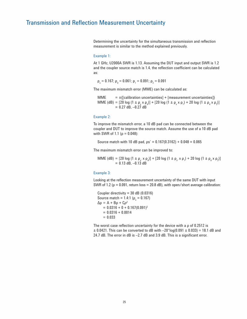
Determining the uncertainty for the simultaneous transmission and reflection

measurement is similar to the method explained previously.

Example 1:

At 1 GHz, U2000A SWR is 1.13. Assuming the DUT input and output SWR is 1.2

and the coupler source match is 1.4, the reflection coefficient can be calculated

as:

ρs = 0.167; ρ

d = 0.061; ρ

1 = 0.091; ρ

2 = 0.091

The maximum mismatch error (MME) can be calculated as:

MME = ±{[calibration uncertainties] + [measurement uncertainties]}

MME (dB) = [20 log (1 ± ρs x ρ

d)] + [20 log (1 ± ρ

s x ρ

1) + 20 log (1 ± ρ

d x ρ

2)]

= 0.27 dB, –0.27 dB

Example 2:

To improve the mismatch error, a 10 dB pad can be connected between the

coupler and DUT to improve the source match. Assume the use of a 10 dB pad

with SWR of 1.1 (ρ = 0.048):

Source match with 10 dB pad, ρs’ = 0.167(0.3162) + 0.048 = 0.065

The maximum mismatch error can be improved to:

MME (dB) = [20 log (1 ± ρs’ x ρ

d)] + [20 log (1 ± ρ

s’ x ρ

1) + 20 log (1 ± ρ

d x ρ

2)]

= 0.13 dB, –0.13 dB

Example 3:

Looking at the reflection measurement uncertainty of the same DUT with input

SWR of 1.2 (ρ = 0.091, return loss = 20.8 dB), with open/short average calibration:

Coupler directivity = 30 dB (0.0316)

Source match = 1.4:1 (ρs = 0.167)

∆ρ = A + Bρ + Cρ2

= 0.0316 + 0 + 0.167(0.091)2

= 0.0316 + 0.0014

= 0.033

The worst case reflection uncertainty for the device with a ρ of 0.2512 is

± 0.0421. This can be converted to dB with –20*log(0.091 ± 0.033) = 18.1 dB and

24.7 dB. The error in dB is –2.7 dB and 3.9 dB. This is a significant error.

26

Transmission and Reflection Measurement Uncertainty

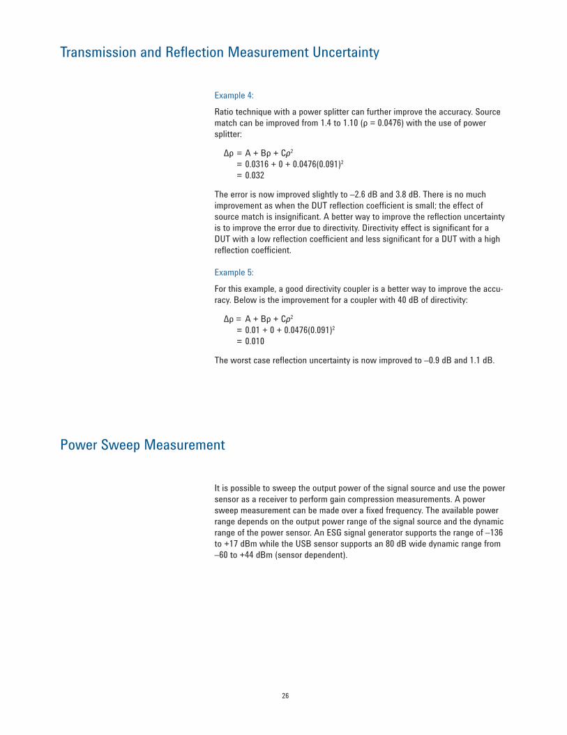
Example 4:

Ratio technique with a power splitter can further improve the accuracy. Source

match can be improved from 1.4 to 1.10 (ρ = 0.0476) with the use of power

splitter:

∆ρ = A + Bρ + Cρ2

= 0.0316 + 0 + 0.0476(0.091)2

= 0.032

The error is now improved slightly to –2.6 dB and 3.8 dB. There is no much

improvement as when the DUT reflection coefficient is small; the effect of

source match is insignificant. A better way to improve the reflection uncertainty

is to improve the error due to directivity. Directivity effect is significant for a

DUT with a low reflection coefficient and less significant for a DUT with a high

reflection coefficient.

Example 5:

For this example, a good directivity coupler is a better way to improve the accu-

racy. Below is the improvement for a coupler with 40 dB of directivity:

∆ρ = A + Bρ + Cρ2

= 0.01 + 0 + 0.0476(0.091)2

= 0.010

The worst case reflection uncertainty is now improved to –0.9 dB and 1.1 dB.

Power Sweep Measurement

It is possible to sweep the output power of the signal source and use the power

sensor as a receiver to perform gain compression measurements. A power

sweep measurement can be made over a fixed frequency. The available power

range depends on the output power range of the signal source and the dynamic

range of the power sensor. An ESG signal generator supports the range of –136

to +17 dBm while the USB sensor supports an 80 dB wide dynamic range from

–60 to +44 dBm (sensor dependent).

27

Optimizing Measurement Speed

For applications that require fast measurement speed, it is possible to achieve

15 ms per reading using P-Series power meters and sensors with external

triggering power or frequency sweep capability. This feature allows the signal

source to trigger the power meter via an external TTL signal for measurement

capture. After measurement is captured, the power meter outputs a trigger sig-

nal to the signal source to continue with the next step point. This sequence is

repeated for every step point. The two way communication via hardwire connec-

tions between these two instruments helps to reduce communication overhead

between these two instruments, resulting in overall test time improvement.

Figure 26 illustrates the configuration for this test setup. Please refer to Agilent

application note “Maximizing Measurement Speed Using P-Series Power

Meters” (literature number 5989-7678EN) for more details on how to enable this

feature. The demonstration software also provides step-by-step instructions on

how to setup this measurement.

Figure 26. Fast scalar network analysis using Agilent P-Series power meters and sensors

GPIB to GPIB connection

Transmitted, B

Directional coupler

Power splitter

DUT


Trig Out Trig In

Trig OutTrig In

Trig In

GPIB to GPIB connection

Incident, R

Reflected, A

28

Summary

The U2000 Series sensor based scalar network analyzer offers the ability to per-

form accurate transmission and reflection measurements in addition to general

purpose power measurements. The USB sensor offers wide dynamic range and

provides accuracy up to 3%. The frequency response is less than 0.1 dB with

calibration factor corrections. When used together with a power splitter and

coupler, it enables accurate scalar power measurements with low overall setup

cost.

Transmission measurements such as 3 dB bandwidth of a bandpass filter, gain,

and return loss of an amplifier, return loss of an antenna, flatness of a low pass

filter, and frequency response of a cable can be easily made with the U2000

Series based SNA with the help of a simple software.

29

Agilent power metersN1913A/14A EPM Series power meters

E4416A/17A EPM-P Series power meters

N1911A/12A P-Series power meters

U2000 Series USB power sensors

Agilent power sensors

POWER METERS

E441

6/17

A

N19

13/

14A

N19

11/

12A

N82

62A

Product Description /Sensor Tech.

FrequencyRange Power Range

PO

WER

SEN

SO

RS

N8480 / 8480 Series Thermocouple and Diode sensors

N848xA √ √ √ Thermocouple Power Sensor 100 kHz to 67 GHz –35 dBm (316 µW) to +20 dBm (100 mW)

N848xB/H √ √ √ High Power Thermocouple Sensor 100 kHz to 18 GHz –15 dBm (100 µW) to +44 dBm (25 W)

848xD √ √ √ Diode Power Sensor 100 kHz to 50 GHz –70 dBm (100 pW) to –20 dBm (10µW)

CW sensors E441xA √ √ √ Diode Power Sensor 10 MHz to 33 GHz –70 dBm (100 pW) to +20 dBm (100 mW)

E9300 Series average sensorsE930xA √ √ √ Diode Power Sensor 9 kHz to 24 GHz –60 dBm (1 nW) to +20 dBm (100 mW)

E930xB/H √ √ √ Diode Power Sensor 10 MHz to 18 GHz –50 dBm (10 nW) to +44 dBm (25 W)

E9320 Series peak and average sensors E932xA √ – √ Diode Power Sensor 50 MHz to 18 GHz –60 dBm (1 nW) to +20 dBm (100 mW)

P-Series wideband sensorsN1921A – – √ Diode Power Sensor 50 MHz to 18 GHz –35 dBm (316 nW) to +20 dBm (100 mW)

N1922A – – √ Diode Power Sensor 50 MHz to 40 GHz –35 dBm (316 nW) to +20 dBm (100 mW)

U2000 USB sensors

U200xA – √ – Diode Power Sensor 9 kHz to 26.5 GHz –60 dBm (1 nW) to +20 dBm (100 mW)

U200xB – √ – Diode Power Sensor 10 MHz to 18 GHz –30 dBm (1 µW) to +44 dBm (25 W)

U200xH – √ – Diode Power Sensor 10 MHz to 24 GHz –50 dBm (10 nW) to +44 dBm (25 W)

8480 waveguide sensors

R8486D √ √ √ Waveguide Power Sensor 26.5 GHz to 40 GHz –70 dBm (100 pW) to –20 dBm (10 µW)

Q8486D √ √ √ Waveguide Power Sensor 33 GHz to 50 GHz –70 dBm (100 pW) to –20 dBm (10 µW)

N8486AR √ √ √ Thermocouple Waveguide Power Sensor 26.5 GHz to 40 GHz –35 dBm (316 µW) to +20 dBm (100 mW)

N8486AQ √ √ √ Thermocouple Waveguide Power Sensor 33 GHz to 50 GHz –35 dBm (316 µW) to +20 dBm (100 mW)

V8486A √ √ √ V-band Power Sensor 50 GHz to 75 GHz –30 dBm (1 µW) to +20 dBm (100 mW)

W8486A √ √ √ Waveguide Power Sensor 75 GHz to 110 GHz –30 dBm (1 µW) to +20 dBm (100 mW)

Ordering Information

30

Ordering Information

Agilent power splitters11667A DC to 18 GHz power splitter

11667B DC to 26.5 GHz power splitter

11667C DC to 50 GHz power splitter

Agilent signal generatorsAgilent ESG, MXG and PSG signal generators

Agilent couplers and bridges

Model Frequency range Directivity Nominal coupling Insertion loss86205A 300 kHz to 6 GHz < 30 dB to 5 MHz

< 40 dB to 2 GHz

< 30 dB to 3 GHz

< 20 dB to 5 GHz

< 16 dB to 6 GHz

16 dB < 1.5 dB

86207A 300 kHz to 3 GHz < 30 dB to 5 MHz

< 40 dB to 1.3 GHz

< 35 dB to 2 GHz

< 30 dB to 3 GHz

15 dB < 1.5 dB

87300B 1 to 20 GHz > 16 dB 10 ± 0.5 dB < 1.5 dB

87300C 1 to 26.5 GHz > 14 dB to 12.4 GHz

> 12 dB to 26.5 GHz

10 ± 1.0 dB < 1.2 dB to 12.4 GHz

< 1.7 dB to 26.5 GHz

87300D 6 to 26.5 GHz > 13 dB 10 ± 0.5 dB < 1.3 dB

87301B 10 to 46 GHz > 10 dB 10 ± 0.7 dB < 1.9 dB

87301C 10 to 50 GHz > 10 dB 10 ± 0.7 dB < 1.9 dB

87301D 1 to 40 GHz > 14 dB to 20 GHz

>10 dB to 40 GHz

13 ± 1.0 dB < 1.2 dB to 20 GHz

< 1.9 dB to 40 GHz

87301E 2 to 50 GHz > 13 dB to 26.5 GHz

>10 dB to 50 GHz

10 ± 1.0 dB < 2.0 dB

773D 2 to 18 GHz > 30 dB to 12.4 GHz

> 27 dB to 18 GHz

20 ± 0.9 dB < 0.9 dB

Broadband couplers are also available from manufacturers belowNarda Microwave-East. www.nardamicrowave.com

Krytar. www.krytar.com

Quinstar Technology Inc. www.quinstar.com

Agilent calibration kitsAgilent offers a variety of mechanical calibration kits ranging from DC to 110GHz. For more information, refer to URL:

www.home.agilent.com/agilent/product.jspx?cc=US&lc=eng&ckey=1000000298:epsg:pgr&nid=-536902686.0.00&id=1000000298:epsg:pgr&pselect=SR.GENERAL#16

31

References

[1] Agilent Application Note 183 High Frequency Swept Measurements, December 1978

[2] Scalar Measurement Fundamentals, Hewlett Packard’s Scalar Measurement Seminar

[3] Scalar Measurements with the ESA-L1500A 1.5 GHz Spectrum Analyzer and Tracking Generator, Product Note,

literature number 5966-1650E

Related Agilent Literature

Publication title Pub number

Agilent N1911A/N1912A P-Series Power Meters and N1921A/N1922A Wideband Power Sensors

Data Sheet5989-2471EN

Agilent U2000 Series USB Power Sensors Data Sheet 5989-6278EN

Agilent E4416A/E4417A EPM-P Series Power Meters and E-Series E9320 Peak and Average

Power Sensors Data Sheet5980-1469E

Agilent N1913A and N1914A EPM Series Power Meters Data Sheet 5990-4019EN

Agilent E4418B/E4419B EPM Series Power Meters, E-Series and 8480 Series Power Sensors

Data Sheet5965-6382E

Agilent N8480 Series Thermocouple Power Sensors Data Sheet 5989-9333EN

Agilent Choosing the Right Power Meter and Sensor Product Note 5968-7150E

Agilent Fundamentals of RF and Microwave Power Measurements Application

Notes 1449-1/2/3/45988-9213/4/5/6EN

Agilent P-Series Power Sensor Internal Zeroing and Calibration for RF Power Sensors

Application Note5989-6509EN

Agilent Maximizing Measurement Speed Using P-Series Power Meters Application Note 5989-7678EN

Agilent RF and Microwave Test Accessories Selection Guide 5990-5499EN

32

Appendix

For your reference, this appendix shows the SCPI commands used in the demonstration software to control the signal

generator and power meter for automated scalar network analysis.

Configure the U2000 Series USB sensor:

SYST:PRES //Preset the sensor

Wait for 1s

INIT:CONT OFF //Set to single trigger

SENS:MRATE NORM //Set to normal measurement rate

SENS:AVER:COUN 1 //Set filter length to one

SENS:AVER ON //Turn on averaging

CAL:ZERO:TYPE EXT //Set to external zeroing

CAL //Zeroing the sensor

while value not equals to zero

{

value = STAT:OPER:CAL:COND? //Return 0 when zeroing completed

}

Configure signal generator:

SYST:PRES //Preset the instrument

Wait for 1s

POW:LEVEL 10DBM //Set source power to 10 dBm

OUTP:STAT ON //Turn on source power

Step through a range of frequency using these commands to perform scalar frequency sweep measurement:

FREQ 1GHz //Send this command to source to set source frequency to 1 GHz

SENS:FREQ 1GHz //Send this command to sensor to set sensor frequency to 1 GHz

READ? //Send this command to sensor to read the input power of sensor

Move to next frequency point and repeat above steps.

www.agilent.com

Agilent Email Updates

www.agilent.com/find/emailupdates

Get the latest information on the

products and applications you select.

www.lxistandard.org

LAN eXtensions for Instruments puts

the power of Ethernet and the Web

inside your test systems. Agilent

is a founding member of the LXI

consortium.

Agilent Channel Partners

www.agilent.com/find/channelpartners

Get the best of both worlds: Agilent’s

measurement expertise and product

breadth, combined with channel

partner convenience.

www.axiestandard.org

AdvancedTCA® Extensions for

Instrumentation and Test (AXIe) is

an open standard that extends the

AdvancedTCA® for general purpose

and semiconductor test. Agilent

is a founding member of the AXIe

consortium.

http://www.pxisa.org

PCI eXtensions for Instrumentation

(PXI) modular instrumentation

delivers a rugged, PC-based high-

performance measurement and

automation system.

Agilent Advantage Services is com-

mitted to your success throughout

your equipment’s lifetime. We share

measurement and service expertise

to help you create the products that

change our world. To keep you com-

petitive, we continually invest in tools

and processes that speed up calibra-

tion and repair, reduce your cost of

ownership, and move us ahead of

your development curve.

www.agilent.com/quality

www.agilent.com/find/advantageservices

For more information on Agilent Technologies’ products, applications or services, please contact your local Agilent

office. The complete list is available at:

www.agilent.com/find/contactus

AmericasCanada (877) 894 4414 Brazil (11) 4197 3500Mexico 01800 5064 800 United States (800) 829 4444

Asia PacificAustralia 1 800 629 485China 800 810 0189Hong Kong 800 938 693India 1 800 112 929Japan 0120 (421) 345Korea 080 769 0800Malaysia 1 800 888 848Singapore 1 800 375 8100Taiwan 0800 047 866Other AP Countries (65) 375 8100

Europe & Middle EastBelgium 32 (0) 2 404 93 40 Denmark 45 70 13 15 15Finland 358 (0) 10 855 2100France 0825 010 700* *0.125 €/minute

Germany 49 (0) 7031 464 6333 Ireland 1890 924 204Israel 972-3-9288-504/544Italy 39 02 92 60 8484Netherlands 31 (0) 20 547 2111Spain 34 (91) 631 3300Sweden 0200-88 22 55United Kingdom 44 (0) 118 9276201

For other unlisted Countries: www.agilent.com/find/contactusRevised: October 14, 2010

Product specifications and descriptions in this document subject to change without notice.

© Agilent Technologies, Inc. 2011Printed in USA, April 28, 20115990-7540EN

Documents

Scalar Network Analysis with U2000 Series USB … Network Analysis with U2000 Series USB Power Sensors Application Note Overview The Agilent U2000 Series USB power sensor is a compact,