SATELLITE APPLICATION FACILITY ON SUPPORT TO OPERATIONAL HYDROLOGY AND WATER MANAGEMENT

(H-SAF)

VISITING SCIENTIST ACTIVITY IN SUPPORT OF WP 2400 VS 310 PROGRAMME

ACTIVITY REPORT

Generation of an European Cloud-Radiation Database to be used for PR-OBS-1

(Precipitation Rate at Ground by MW Conical Scanners)

Alberto Mugnai, Daniele Casella, Marco Formenton, Paolo Sanò

Istituto di Scienze dell’Atmosfera e del Clima (ISAC) Consiglio Nazionale delle Ricerche (CNR)

Roma, Italy

Gregory J. Tripoli, Wing Yee Leung

Department of Atmospheric and Oceanic Sciences The University of Wisconsin Madison, Wisconsin, USA

Eric. A. Smith, Amita Mehta

NASA / Goddard Space Flight Center Greenbelt, Maryland, USA

2

INDEX

FOREWORD 3 1. INTRODUCTION 4 2. METHODOLOGY 6

2.1 Description of the Models 6 2.1.1 Cloud Resolving Model 6 2.1.2 Radiative Transfer Model 6

Radiometer Model 8 Surface Emissivity Models 8 Single-Scattering Models 8

2.2 Generation of the CRD / CDRD Databases 9 2.3 The CDRD Retrieval Algorithm 13

3. ANALYSIS 17 3.1 Database Content and Statistics 17

3.1.1 Microphysical Quantities 17 3.1.2 Upwelling Brightness Temperatures 20 3.1.3 Relationships between Microphysical Quantities and Upwelling Brightness Temperatures 24 3.1.4 Comparison of Measured and Simulated Brightness Temperatures 25

3.2 An Application of the CDRD Algorithm 30 4. SUMMARY AND CONCLUSIONS 35 5. REFERENCES 37

3

FOREWORD The activity that is described in this Report was made possible and supported by the Visiting Scientist Programme of the Development Phase of EUMETSAT’s Project “Application Facility on Support to Operational Hydrology and Water Management” (H-SAF). The activity was planned by the three principal investigators of the Cloud Dynamics and Radiation Database (CDRD) project – Dr. Alberto Mugnai of the Institute of Atmospheric Sciences and Climate (ISAC) of the Italian National Research Council (CNR) of Rome, Italy; Prof. Eric Smith of the NASA / Goddard Space Flight Center (GSFC) of Greenbelt, Maryland, USA; and Prof. Gregory Tripoli of the University of Wisconsin (UW) of Madison, Wisconsin, USA. All details were examined and established in May-June 2008 during a visit of Prof. Tripoli and Ms. Wing Yee Leung of UW to the CNR-ISAC Group of Satellite Meteorology in Rome (Dr. Mugnai, Dr. Daniele Casella, Dr. Marco Formenton and Dr. Paolo Sanò) which is responsible for developing H-SAF product PR-OBS-1. The necessary model simulations were initiated at that time, then continued by the ISAC-Roma Group of Satellite Meteorology, and finally further enhanced during a second visit of Ms. Leung during November-December 2009. All subsequent analyses that are discussed in this Report have been carried out by the ISAC-Roma Group of Satellite Meteorology in cooperation with Prof. Tripoli and Ms. Leung of UW and with Prof. Smith and Dr. Amita Mehta of NASA/GSFC. The objective of the Visiting Scientist activity was to generate a statistically significant Cloud-Radiation Database (CRD) / Cloud Dynamics and Radiation Database (CDRD) for the European region to be used within the H-SAF project as an input to a physical-statistical profile-based Bayesian algorithm (the CDRD Algorithm) for precipitation retrieval from conically-scanning microwave radiometers – H-SAF product PR-OBS-1. To this end, a large number (sixty) of simulations of different precipitation events over the European area for the March 2006 – February 2007 one-year period have been performed by means of the cloud resolving model University of Wisconsin – Non-hydrostatic Modeling System (UW-NMS), in such a way to take into account the various climatic regions, types of precipitation and seasonal variations. The activity consisted of a development phase and an operational phase. In the development phase – that basically took place during the afore-mentioned visits – the UW-NMS model was implemented at CNR-ISAC and the European CRD was expanded so as to cover a full year period. In addition, tests on the dynamical/environmental variables to be included in the CDRD were performed. In the operational phase – that basically lasted one year – generation of the European CRD was completed. In addition, the studies on the dynamical/environmental variables to be included in the CDRD were concluded. The new version of the European CRD was delivered together with version 2 of the algorithm for product PR-OBS-1. On the other hand, the European CDRD will need further studies, model simulations and precipitation retrieval tests and analyses, before it can be delivered for operational use within H-SAF.

4

1. INTRODUCTION Determining precipitation rate at the ground from the few channels of SSM/I is an extremely ill-conditioned problem. Precipitation at the ground can not be directly observed from space, however, in principle it can be derived from knowledge of the cloud microphysical structure along the direction of sight. SSMIS includes more information on the atmospheric structure, but not as cloud microphysics is concerned. Consequently, information relating cloud microphysics to observations from satellite-borne microwave (MW) radiometers needs to be input from external sources. For PR-OBS-1 we proposed to derive such microphysical information from a Cloud Resolving Model (CRM). A shortcoming of this approach is that it is currently not possible to run these models in-line with the flow of satellite data. It is therefore necessary to run the CRM off-line for a number of well-documented events (generally, results of re-analysis exercises) and collect the results in a database. Then, in a post analysis phase, a detailed Radiative Transfer Model (RTM), as it is particularly necessary when ice is involved in the precipitation event, is applied to the CRM output to compute the upwelling brightness temperatures (TBs) that would be measured by a satellite-borne MW radiometer. The collection of cloud and precipitation microphysical profiles for a series of different CRM simulations and of the associated TBs at the instrument (SSM/I & SSMIS) channel frequencies constitutes the Cloud-Radiation Database (CRD). Precipitation retrieval for PS-OBS-1 is performed by means of a physical-statistical profile-based Bayesian algorithm that has been developed and is continuously being improved at CNR-ISAC. The algorithm makes use of the CRD to search for the most probable profile(s) according to the proximity of measured and modelled TBs and on a priori probabilities of occurrence of the various profile structures. Surface rain rates are computed by means of the model rain rates for the solution hydrometeor profiles. The first version of the CNR-ISAC algorithm that has been used within the H-SAF project, was published with the name of Bayesian Algorithm for Microwave Precipitation Retrieval (BAMPR) – see Mugnai et al. (2001); Di Michele et al. (2003, 2005); Tassa et al. (2003, 2006). The BAMPR algorithm was characterized by a detailed description of the estimation uncertainties, a careful coupling of the forward and inverse problem and a quantitative evaluation of the representativeness of the cloud-radiation database. As shown by Panegrossi et al. (1998), precision and accuracy of the precipitating cloud structure estimation, and hence of the surface rainfall rate retrieval, are strictly related to the appropriate generation of the cloud profile dataset associated to the typology of the observed precipitation event more than to an a-posteriori statistical treatment of uncertainties. Thus, it is important to use several cloud model simulations for different types of precipitation systems and to generate the corresponding cloud-radiation databases, in order to specialize the algorithm to different storm structures. In essence, the algorithm performance can be improved by generating a statistically significant CRD by means of a large number of different CRM simulations representing all precipitation regimes that occur in the zone and season under investigation. Despite some reasonable successes with the CRD and the Bayesian approach, there is a considerable reservoir of potential information available that is not usually tapped. This ancillary information exists in the knowledge of the “synoptic situation” of the

5

considered event and the geographical and temporal location of the event. This knowledge renders some entries into the CRD more relevant than others by virtue of how similar the circumstances of the simulated event are to those of the event for which the database is applied. We can capture this information in the form of “dynamical tags” which can be used to link a satellite-observed event to a subset of the entire CRD using an independent estimate of these tags always available from short-term model forecast products, such as the Global Forecasting System (GFS) model of the National Oceanic and Atmospheric Administration (NOAA). Here the term “dynamical tags” actually refers not only to ancillary dynamics information such as geostrophic forcing or frontal lifting, but also thermodynamic, hydrodynamic and geographical information. To accomplish this, the CRD must be expanded to include these “dynamical tags”. The expanded CRD is called the Cloud Dynamics and Radiation Database (CDRD) (Mugnai et al., 2006). We are presently testing a new passive microwave precipitation retrieval algorithm which employs these tags – thus, called the CDRD Algorithm.

To generate the CRD (or CDRD) to be used for PR-OBS-1, we make use of the CRM University of Wisconsin – Non-hydrostatic Modeling System (UW-NMS), developed by Prof. Gregory J. Tripoli – see Tripoli (1992) and Tripoli and Smith (2008). The ultimate goal is to generate a CRD / CDRD that covers all climatic regions, types of precipitation and seasonal variations that can occur in the European area. Thus, the European CRD / CDRD that we have developed for use in the H-SAF project is formed by a large number (60) of UW-NMS simulations over the European area and the associated upwelling TBs at SSM/I and SSMIS frequencies. In addition, in order to cover all possible precipitation regimes in the European area and not to generate any bias towards preferential precipitation regimes, time and position of every simulation have been chosen by an analysis of the synoptic situation over the European area within the one-year period March 2006 – February 2007.

6

2. METHODOLOGY

2.1 Description of the Models

2.1.1 Cloud Resolving Model The UW-NMS is a three-dimensional (3-D), time-dependent cloud/mesoscale numerical model capable of simulating atmospheric phenomena with horizontal scales ranging from the microscale (turbulence) to the synoptic scale (extratropical cyclones, fronts, etc.). It is based on the non-Boussinesq quasi-compressible dynamical equations. Model thermodynamics are based on the prediction of a moist ice-liquid entropy variable, designed to be conservative over all ice and liquid adiabatic process (Tripoli and Cotton, 1981). Dynamic properties of flow such as vorticity, kinetic energy and potential enstrophy are conserved by the advection scheme in the UW-NMS. The model uses variable step topography capable of capturing steep topographical slopes, while at the same time accurately representing subtle topography variations. Conservation equations for the specific humidity of total water and several ice and liquid water hydrometeor categories are also included. The model is formulated on a two-way multiply nested Arakawa “C” grid system, cast on a rotated spherical grid system. The grid system includes multiple 2-way nesting capability to allow locally enhanced resolutions. The nesting system mod can be programmed to move along a specified trajectory or to move with a predicted variable such as a surface pressure minimum. The microphysical module used in the UW-NMS version utilized within H-SAF, is a modified form of the scheme described by Flatau et al. (1989) and Cotton et al. (1986). Specifically, in UW-NMS the treatment of ice categories and specifics of the precipitation physics tendencies have been modified from the original published works to enhance their performance. The microphysics is a bulk microphysics parameterization, which includes six hydrometeor categories labelled as: 1) suspended cloud droplets, 2) precipitating rain drops, 3) suspended pristine ice crystals, and precipitating 4) ice aggregates, 5) low-density graupel particles (or snow) and 6) high density graupel particles. Depending on the application, all or some of these categories may be selected. Any combination of frozen and liquid hydrometeors can coexist within the same grid volume at any given time to allow hydrometeor category interaction to take place.

2.1.2 Radiative Transfer Model In order to simulate the upwelling brightness temperatures (TBs) to be included in the database, we have to apply a radiative transfer (RT) code to the microphysical outputs of the simulated precipitation events and compute the upwelling radiances over the simulated satellite footprints. To this end, fully 3-D RT schemes should be used. However, these schemes are computationally heavy, and fully rely on the macrophysical structure of the cloud model simulation. Thus, it is customary to resort to simpler one-dimensional (1-D) plane-parallel schemes, which are much faster – though less accurate. We have used a 3-D adjusted plane parallel RT scheme, which has been developed by

7

Roberti et al. (1994) (see also Liu et al., 1996; Bauer et al., 1998; Tassa et al., 2003). In this approach, the plane-parallel cloud structures are generated from the cloud model paths along the radiometer direction of sight, rather then from the vertical cloud model columns. The RT is therefore performed along a slanted profile in the direction of observation of the radiometer. Remarkably, the downward flux is computed through the cloud structure along the specular line reflected at the surface, a fact that may have a significant effect at cloud edges at low frequencies. This method is computationally efficient, and accounts for the geometrical errors that a complete 1-D RT scheme is prone to, partially reducing errors in radiative transfer modelling. However, pure 3-D radiative effects are neglected, since the radiation is still trapped inside the slanted (and reflected) column, and in case of enhanced horizontal inhomogeneities, the scheme may produce significant discrepancies with the results obtained with a fully 3D model. The performances of the slanted-path plane-parallel RT approximation have been deeply investigated by several authors (Roberti et al., 1994; Bauer et al., 1998; Kummerow, 1993) who generally agree on the errors being limited to a few K on average scenes, even though local values may be important in case of large horizontal gradients (e.g., at the cloud edges) (see Liu et al., 1996; Czekala et al., 2000; Olson et al., 2001). Once the monochromatic upwelling radiances have been computed at high resolution (i.e., at the resolution of the CRM model – 2 km) for the full cloud model domain, the upwelling TBs at sensor resolution (i.e., that would be observed by a real radiometer) are computed for each channel using the instrument transfer function: i.e., by first integrating the monochromatic upwelling radiances over the channel-width, taking into account the channel spectral responsivity, and then integrating the channel upwelling radiances over the field of view (i.e., over all cloud-model pixels that are contained in the field of view), taking into account the radiometer antenna pattern and radiometric noise. Then, the corresponding high-resolution hydrometeor liquid/ice water content profiles, as well as the corresponding precipitation rate profiles for both rain and ice, are extracted from the cloud model simulation and averaged over the field of view to produce the same quantities at sensor resolution. A key point of this process concerns the definition of the cloud structures which have to be associated to the simulated TBs. In principle, for each channel a different cloud structure – (basically) filling up the slanted elliptical cylinder with sizes corresponding to the cross-track and along-track resolutions of the considered channel – should be associated with each TB point of the database. This strategy, however, would make the multi-frequency retrieval rather complex and not univocal. The simplest choice is therefore to choose a common single resolution for the microphysical parameters belonging to the cloud-radiation database. We usually associate slanted cloud structures corresponding to the resolution of the 89 GHz frequency as a reasonable compromise. Some of the outputs of the CRM simulations are inputs for the radiative transfer model (RTM) in order to generate the upwelling TBs. In detail, these quantities are the vertical profiles of the liquid/ice water contents (LWC and IWC, respectively) of the various hydrometeors, together with the surface temperature and the temperature / moisture profiles.

8

Other inputs to the RTM are: the radiometer model, the surface emissivity model, and the single-scattering model.

Radiometer model The radiometer model is a secondary input to the RT model and specifies all characteristics of the radiometer that has to be simulated – i.e. frequency, polarization and width of the candidate channels; viewing angle of the radiometer; field of view and antenna pattern of the various channels. In principle, an Instrument Transfer Function has to be defined for each channel in order to compute the upwelling TBs from the upwelling monochromatic radiances. For this study, we have used the channel characteristics of the following conically-scanning radiometers:

• Special Sensor Microwave Imager (SSM/I) • Special Sensor Microwave Imager (SSMIS) • TRMM Microwave Imager (TMI) • Advanced Microwave Scanning Radiometer-EOS (AMSR-E)

Surface Emissivity Models Surface emissivity impacts the upwelling TBs especially at the lower window frequencies. It depends on frequency and polarization, observation geometry, and surface characteristics (land / ocean, surface roughness, type of soil and soil cover, soil humidity, etc.). Thus, we have selected three different surface emissivity models to best represent the different surface backgrounds of the selected CRM simulations. The three surface emissivity models that have been implemented, are: • For land surfaces, the forest and agricultural land surface emissivity by Hewison

(2001); • For a sea surface, the fast and accurate ocean emissivity model of English and

Hewison (1998) (see also Hewison and English, 2000 and Schluessel et al, 1998), which provides accurate estimates of surface emissivity between 10 and 200 GHz for view angles up to 60° and wind speeds from 0 to 20 m/s;

• For snow covered surfaces, the snow emissivity model that has been empirically derived by Hewison (1999) from satellite retrievals and ground-based measurements; in particular, five different snow cover types have been considered that cover the full range of snow emissivity presented by the previous authors – i.e., forest +snow, deep dry snow, fresh wet snow, frozen soil, first year ice, compact snow.

Single-Scattering Models Computation of the single-scattering properties of the various hydrometeor species is straightforward if only pure water and ice spheres are considered (i.e., for Mie scattering), but can be a major challenge for natural ice hydrometeors (especially for snowflakes and ice aggregates) due to their wide variety of sizes, densities, and shapes. Since information on shape is not available from the UW-NMS microphysical parameterization scheme, we have to take some assumptions; i.e.: • Liquid (cloud and rain) particles are assumed to be spherical and homogeneous, and

9

therefore their scattering properties are computed by means of Mie theory (Bohren and Huffman, 1983) using an efficient code developed by Wiscombe (1980).

• Graupel particles are assumed to be spherical with densities nearly that of pure ice (0.9 g cm-3); they are assumed to be “equivalent homogeneous spheres” having an effective dielectric function obtained by combining the dielectric functions of ice and air (or water, in case of melting) according to the effective medium Maxwell-Garnett mixing theory for a two-component mixture of inclusions of air (water) in an ice matrix (see Bohren and Huffman 1983). As a consequence, Mie theory is used even in this case.

• Pristine ice particles are highly non-spherical, and we chose to use the Grenfell and Warren (1999) approximation (see also Neshyba et al. 2003). The single-scattering properties of each nonspherical ice particle are computed by means of a collection of ns equal-size solid-ice spheres having a diameter determined by the volume to cross-sectional area ratio (V/A) of the original nonspherical ice particle. The volume (V) is provided by the UW-NMS simulations. For calculating the cross-sectional area (A), we use the observational relationship A / (πD2/4) = C0 DC that has been published by Heymsfield and Miloshevich (2003) for several different individual particle habits – here, D (in cm) is the maximum diameter of the particle, while the coefficients C0 and C (in appropriate cgs units) depend on ice particle habit. For pristine ice crystals we use values C0 = 0.18 and C = 0.2707, that are indicated by the same authors as appropriate averages for midlatitude, continental mixed-habit cirrus clouds. As a result, the diameter (Ds) and the number (ns) of the equivalent solid-ice spheres are given by:

C 0ice

s D CD

ρρD =

3s

C30

s D D

C1Cn

+

−=

where, ρice = 0.916 g cm-3 while the density ρ of the pristine ice crystals is usually equal to 0.1 g cm-3.

• Snowflakes and ice aggregates are low-density, fluffy ice particles (as long as they are completely frozen) that can not be modelled according to Maxwell-Garnett mixing theory – the resulting “equivalent homogeneous soft-ice spheres” would have, according to Mie theory, very large asymmetry factors (> 0.9) at the higher microwave frequencies and would not adequately “cool” the upwelling radiation. To overcome this problem, we used the Surussavadee (2006) model in which non-spherical scattering results were fitted using Mie calculations for spheres having a density that is a function of the wavelength.

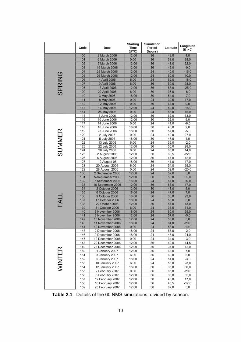
2.2 Generation of the CRD / CDRD Databases To generate the CRD / CDRD databases for the European region to be used within the H-SAF project, sixty simulations of different precipitation events over the European area for the March 2006 – February 2007 one-year period were performed by means of the cloud resolving model UW-NMS, in such a way to take into account the various climatic regions, types of precipitation and seasonal variations. Table 2.1 provides the details of all simulations. Figure 2.1 shows their inner domains.

10

Code Date

Starting Time (UTC)

Simulation Period (hours)

Latitude Longitude (E > 0)

100 2 March 2006 12.00 36 48,0 4,0 101 6 March 2006 0.00 36 38,0 28,0 102 9 March 2006 12.00 36 48,0 22,0 103 19 March 2006 12.00 36 42,0 -9,0 104 25 March 2006 12.00 24 40,0 -15,0 105 26 March 2006 12.00 24 50,0 10,0 106 4 April 2006 6.00 24 62,0 -18,0 107 9 April 2006 6.00 36 59,0 28,0 108 13 April 2006 12.00 36 65,0 -25,0 109 22 April 2006 6.00 30 36,0 -6,0 110 3 May 2006 18.00 30 54,0 -7,0 111 8 May 2006 0.00 24 30,5 17,0 112 12 May 2006 0.00 36 63,0 0,0 113 16 May 2006 12.00 24 50,0 -15,0

SP

RIN

G

114 25 May 2006 0.00 24 55,0 15,0 115 5 June 2006 12.00 36 62,0 33,0 116 10 June 2006 12.00 30 35,0 9,0 117 14 June 2006 0.00 24 41,0 -6,0 118 16 June 2006 18.00 30 46,0 2,0 119 23 June 2006 18.00 30 57,0 -5,0 120 2 July 2006 0.00 24 42,0 27,0 121 5-July 2006 18.00 30 47,0 1,0 122 13 July 2006 6.00 24 35,0 -2,0 123 22 July 2006 12.00 36 50,0 28,0 124 28 July 2006 0.00 24 63,0 14,0 125 2 August 2006 12.00 30 60,5 -22,0 126 6 August 2006 12.00 30 47,0 12,0 127 12 August 06 18.00 36 41,0 17,0 128 20 August 2006 6.00 24 54,0 25,0

SU

MM

ER

129 28 August 2006 0.00 24 52,0 -20,0 130 2 September 2006 12.00 24 57,0 5,0 131 5-September 2006 12.00 30 53,0 35,0 132 7 September 2006 18.00 24 57,0 30,0 133 16 September 2006 12.00 36 68,0 17,0 134 2 October 2006 12.00 30 48,0 5,0 135 6 October 2006 18.00 24 47,0 7,0 136 9 October 2006 18.00 36 36,0 23,0 137 17 October 2006 18.00 24 55,0 5,0 138 22 Ocober 2006 12.00 30 57,0 13,0 139 31 October 2006 6.00 24 36,5 31,0 140 5 November 2006 18.00 24 60,0 25,0 141 6 November 2006 12.00 24 57,0 -5,0 142 10 November 2006 12.00 24 53,0 5,0 143 11 November 2006 18.00 24 64,0 -20,0

FALL

144 19 November 2006 0.00 24 53,0 -10,0 145 2 December 2006 18.00 24 53,0 -2,0 146 9 December 2006 18.00 24 45,0 24,0 147 12 December 2006 0.00 24 34,0 -3,0 148 20 December 2006 12.00 36 40,0 14,5 149 23 December 2006 12.00 36 37,0 12,0 150 1 January 2007 12.00 36 63,0 7,0 151 3 January 2007 6.00 36 60,0 5,0 152 5 January 2007 18.00 24 51,0 -3,0 153 10 January 2007 6.00 24 58,0 23,0 154 12 January 2007 18.00 30 35,0 30,0 155 2 February 2007 0.00 36 65,0 -20,0 156 5 February 2007 12.00 36 33,0 35,0 157 12 February 2007 12.00 30 45,0 17,0 158 16 February 2007 12.00 36 43,5 -17,0

WIN

TER

159 23 February 2007 12.00 30 67,0 5,0

Table 2.1: Details of the 60 NMS simulations, divided by season.

11

Figure 2.1: Inner domains of the 60 NMS simulations, divided by season.

In essence, we have generated CRD and CDRD databases for the European region, that cover one entire year from March 1, 2006 to February 28, 2007 and are divided by seasons and equally distributed over them – specifically, for each season there are 15 simulations that are selected in order to make the database as complete as possible (see previous Table 2.1). For each simulation, three nested, concentric and steady grids were used – as schematically shown in Figure2.2. The first and outer grid was set at 50 km resolution, covering a large region of 4550 km x 4550 km (Domain A). The second and intermediate grid was set at 10 km resolution, covering a 910 km x 910 km region (Domain B). The third and inner grid was set at 2 km resolution, covering a 502 km x 502 km region (Domain C). For all grids, 35 vertical levels were used up to about 18 km. Each simulation was run for 24 or 36 hours with a 12-hour spin-up time. This initial period is necessary to better initialize the model by adapting the initial data to the maximum resolution of the model. The NOAA National Centers for Environmental Prediction (NCEP) Global Forecasting System (GFS) gridded analysis fields at about 100 km resolution were used as initial conditions and to nudge the boundaries of the outer grid every six hours throughout the simulation period. After the first 12 hours, the model extracts hydrometeor profiles over the inner domain C – this is done every hour of the remaining simulation time. As an example, Figure 2.3 shows some details of the simulation of an oceanic storm that occurred near the Azores islands on March 25, 2006 (simulation number 104 – see Table 2.1). It is evident that in the synoptical wind pattern of the outer domain (Domain A); a large scale wind convergence triggers strong convection that is aligned along the convergence line itself. Once convection has developed, it exalts convergence with a positive feedback and produces intense convective clouds in the inner grid (Domain C).

12

Figure 2.2: Example of grid nesting design (3 grids for each NMS simulation).

Figure 2.3: NMS simulation of a storm over the Atlantic Ocean (case 104). Left panel:

sea-level wind field in a portion of outer Domain A. Right panel: sea-level wind field and cloud field within inner Domain C.

Then, the simulated upwelling brightness temperatures were computed, following the procedures explained in Section 2.1.1, on the basis of all high-resolution (Domain C) atmospheric and hydrometeor profiles at all one-hour time steps of all 60 simulations.

Domain A Domain C

13

On the other hand, the corresponding dynamical/environmental quantities were extracted at 50 km resolution. In this preliminary version of the CDRD database, we have considered the following dynamical/thermodynamical/microphysical/environmental quantities (hereafter, referred to a “dynamical tags”):

• Freezing Level • Vertical Wind at 700 mb • Vertical Moisture Flux near the Surface (50 mb above the surface) • Convective Available Potential Energy (CAPE) • Positive Vorticity Advection (PVA) at 550 mb • Wind Shear at 300 mb • Surface Height • Lightning Thresholds

2.3 The CDRD Retrieval Algorithm Physically-based (in particular, Bayesian) algorithms for the retrieval of precipitation from satellite-borne microwave radiometers, make use of Cloud Radiation Databases (CRDs) that are composed of thousands of detailed microphysical cloud profiles, obtained from Cloud Resolving Model (CRM) simulations, coupled with the corresponding brightness temperatures (TBs), calculated by applying radiative transfer schemes to the CRM outputs. Usually, CRD’s are generated on the basis of CRM simulations of past precipitation events and then utilized for the analysis of satellite observations of new events. One shortcoming of this CRD approach is that the retrieval of cloud structure and precipitation from a set of multi-frequency TBs is not a unique solution problem. This is because more than one possible configuration of ice and liquid hydrometeors in the horizontal and vertical directions can generate the observed set of TBs – i.e., the simulated cloud structures cannot be distinguished as long as the corresponding TBs remain within the resolution distance from the measured TBs. As an example of this CRD ambiguity, Figure 2.4 shows that many different cloud microphysical structures in the European CRD of previous Section 2.2 have similar TBs at 150 GHz – and therefore can not be distinguished on the basis of this frequency only. Another example is given in Figure 2.5, which shows a 150 GHz vs. 91 GHz scatterplot of all multi-frequency TB vectors of the European CRD. Evidently, several different rain rate values can be found even in small areas of the multi-frequency TB space. Thus, since it is customary to perform some kind of average of all simulated cloud structures that are compatible with the TB measurements, the retrieved microphysical quantities are characterized by large uncertainties and variances. Obviously, this problem depends on the approach itself (the measured TBs do not provide sufficient information) and can be only alleviated by improving the radiometer characteristics or by reducing the approximations and uncertainties that are contained in the cloud model and in the radiative transfer model that have been used to build the database.

14

Figure 2.4: Rain rate (top left), ice rate (top right), columnar liquid water content (bottom left), and columnar ice water content (bottom right) as a function of simulated TBs at 150

GHz in the European CRD database. To facilitate the interpretation of this figure, all different microphysical values corresponding to TB values of 250 ± 10 K are highlighted.

Figure 2.5: 150 GHz vs. 91 GHz scatterplot of all SSMIS simulated TBs in the European CRD (top left). Different colors are used to indicate the rain rate values of the cloud structures corresponding to the 91-150 GHz couples (see color bar). Bottom right

panel emphasizes the ± 10 K region around the point 210 K – 220 K.

15

In addition, when using CRDs that are generated from CRM simulations of past events, microphysical profiles that do not correspond to the actual dynamical/thermodynamical state of the atmosphere at the time of retrieval, may contribute to the retrieval solution – thus, decreasing retrieval accuracy (both in terms of average and variance). In other words, retrieval precision and accuracy is strictly related to the appropriate generation of the cloud profile datasets associated to the typologies of the observed precipitation events more than to an a-posteriori statistical treatment of uncertainties. Thus, the retrieval performance can be improved by generating a statistically significant CRD by means of a large number of different CRM simulations representing all precipitation regimes that are of interest for the zone(s) and season(s) under investigation. However, the non-uniqueness problem remains. This could be further alleviated if MW precipitation retrieval algorithms were designed in such a way to take into account the hydro-thermo-dynamical state of the atmosphere at the time of retrieval. However, this is not usually done by algorithms that are based on the CRD approach. This is quite surprising because despite some reasonable successes with the CRD and the Bayesian approach, there is a considerable reservoir of potential information available that has not been yet tapped. This ancillary information exists in the knowledge of the “synoptic situation” of the considered event and the geographical and temporal location of the event. This knowledge renders some entries into the CRD more relevant than others by virtue of how similar the circumstances of the simulated events are to those of the event for which the database is applied. We can capture this information in the form of “dynamical tags” which can be used to link a satellite-observed event to a subset of the entire CRD using an independent estimate of these tags. To accomplish this, we have expanded the CRD approach so as to include these “dynamical tags”, and have developed a new passive MW precipitation retrieval algorithm which employs these tags, in addition to the upwelling TBs, as further constraints in the selection of profiles from the CRD, that can consequently reduce the retrieval uncertainties. We call these the Cloud Dynamics and Radiation Database (CDRD) approach and the CDRD Algorithm, respectively. The block diagram of our CDRD Bayesian algorithm is shown in Figure 2.6. Specifically: • The TBs measured by SSM/I or SSMIS are first processed (data processing block) in

order to estimate the TB measurements by all different channels at the same geographical position (latitude and longitude) – this is necessary because the low-frequency channels (19, 22, and 37 GHz) have larger footprints than the higher-frequency channels, and therefore a lower number of TBs is measured for them during each swath. Thus, an interpolation procedure is used for the low resolution channels.

• Subsequently, all data are analyzed with a “screening procedure” in order to reject areas (pixels) either having incorrect TB values due to sensor errors, or recognized as areas without rain or with a very low probability of rain.

• Then, the inversion algorithm is applied to each selected pixel. Namely: - a ”Bayesian distance” between the measured multi-frequency TB vector and all

simulated multi-frequency TB vectors of the CDRD database is computed; - in the CDRD version, the Bayesian distance is computed considering not only the

16

TBs but also the values of the dynamical tags; - finally, all selected CDRD profiles are used, with their different Bayesian weights,

to compute the average value of the retrieved surface rain rate and the associated rain rate Bayesian variance.

Figure 2.6: Block diagram of the CDRD Bayesian algorithm.

17

3. ANALYSIS

3.1 Database Content and Statistics The 60 NMS simulations produced about 70 million different high-resolution (2 km) profiles, with about 1 million rainy profiles. These profiles and the associated TBs have been averaged to produce the sensor-resolution (15 km) profiles and the associated TBs that simulate the SSM/I – SSMIS observations. There are about 300.000 of these profiles that contain at least one high-resolution rainy profile. These are the profiles that enter, together with the associated TBs and dynamical tags, in the database. As an example, Table 3.1 shows the components of each profile in the CRD database for SSM/I.

TB19.35V (K) TB37.00H (K) TB19.35H (K) TB85.00V (K) TB22.24V (K) TB85.00H(K) TB37.00V (K) Vert-integrated cloud water path (kg/m**2) Vert-integrated rain water path (kg/m**2) vert-integrated graupel water path (kg/m**2) vert-integrated pristine water path (kg/m**2) vert-integrated snow water path (kg/m**2) vert-integrated aggregates water path (kg/m**2) Surface rain rate (mm/hr) Surface pristine (mm/hr ) Surface aggregate (mm/hr ) Surface graupel (mm/hr ) Surface snow (mm/hr ) Profile number Latitude Longitude Percent land Percent snow Percent ice Height of surface (km) Iztop

Table 3.1: Components of each profile in the CRD database for SSM/I.

3.1.1 Microphysical Quantities Table 3.2 and Figures 3.1 and 3.2 provide some simple statistics of the microphysical properties of the cloud structures of the CRD / CDRD database. It is quite evident that even though the cases of low water/ice contents and low precipitation are the majority, there is a large variability in the cloud microphysical properties which is related to the fact that our simulations attempt to cover the different climatic regions, types of precipitation and seasonal variations that can occur in the European area. Additional brief comments are inserted at the end of table and figure captions.

18

mean variance spread

Cloud Columnar Content (Kg m-2) 0,26 0,12 0 - 5,66 Rain Columnar Content (Kg m-2) 0,34 0,53 0 - 32,95

Graupel Columnar Content (Kg m-2) 0,06 0,18 0 - 18,57 Pristine Ice Columnar Content (Kg m-2) 0,74 2,51 0 - 22,38

Snow Columnar Content (Kg m-2) 0,54 0,56 0 - 5,31 Aggregate Columnar Content (Kg m-2) 0,07 0,04 0 - 10,02

Surface Rain Rate (mm hr-1) 1,11 7,00 0 - 130,69

Table 3.2: Statistics indexes of simulated TBs over land.

Figure 3.1: Probability Distribution Functions (PDFs) of the columnar contents (CC) of

liquid and frozen hydrometeors within the CRD / CDRD European database. Note that all quantities are strongly peaked near 0 kg/m2.

19

Figure 3.2: PDFs of liquid (bottom) and solid (top) precipitation rates at the surface within the CRD / CDRD European database. As observed also in Table 3.2, liquid

precipitation may have very high rates, while solid precipitation is always low.

20

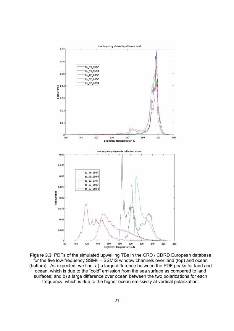
3.1.2 Upwelling Brightness Temperatures Tables 3.3 and 3.4 and Figures 3.3 to 3.5 provide the same statistics for the simulated upwelling TBs for all relevant SSM/I – SSMIS channels within the CRD / CDRD database. Again, large variations may be observed, which are due to the wide range of different meteorological and environmental conditions of the simulated events. Again, additional brief comments are inserted at the end of table and figure captions.

Over land polarization mean variance spread mode tb 19.35GHz V 275 41 220 - 294 279tb 19.35GHz H 271 207 164 - 294 279tb 22.235GHz V 275 24 232 - 293 277tb 37 GHz V 274 25 224 - 293 276tb 37 GHz H 271 104 193 - 293 276tb 85 GHz V 269 85 110 - 294 271tb 85 GHz H 268 106 110 - 294 272tb 91.66 GHz V 269 93 105 - 294 273tb 91.66 GHz H 268 112 105 - 294 273tb 150 GHz V 266 158 92 - 290 273tb 150 GHz H 266 161 92 - 290 273tb 183.31±7 H 242 19 133 - 261 240tb 183.31±3 H 253 31 107 - 272 252tb 183.31±1 H 261 80 96 - 281 263tb 50.3 GHz H 268 39 188 - 285 271tb 52.8 GHz H 258 15 198 - 268 260tb 53.596 GHz H 245 9 210 - 251 246

Table 3.3: Statistics indexes of simulated TBs over land.

Over Ocean polarization mean variance spread mode tb 19.35GHz V 196 122 178 - 266 185tb 19.35GHz H 136 348 98 - 251 118tb 22.235GHz V 219 249 189 - 273 203tb 37 GHz V 222 121 165 - 263 210tb 37 GHz H 170 536 127 - 260 149tb 85 GHz V 256 69 60 - 279 260tb 85 GHz H 232 470 60 - 273 256tb 91.66 GHz V 258 68 59 - 282 259tb 91.66 GHz H 235 453 59 - 274 247tb 150 GHz V 267 80 66 - 290 266tb 150 GHz H 259 144 66 - 289 270tb 183.31±7 H 242 21 81 - 261 239tb 183.31±3 H 253 24 73 - 271 250tb 183.31±1 H 262 45 70 - 282 260tb 50.3 GHz H 235 131 121 - 266 225tb 52.8 GHz H 253 31 135 - 266 247tb 53.596 GHz H 242 23 159 - 252 239

Table 3.4: Statistics indexes of simulated TBs over ocean.

21

Figure 3.3 PDFs of the simulated upwelling TBs in the CRD / CDRD European database

for the five low-frequency SSM/I – SSMIS window channels over land (top) and ocean (bottom). As expected, we find: a) a large difference between the PDF peaks for land and

ocean, which is due to the “cold” emission from the sea surface as compared to land surfaces; and b) a large difference over ocean between the two polarizations for each

frequency, which is due to the higher ocean emissivity at vertical polarization.

22

Figure 3.4: Same as Figure 3.3, but for the high-frequency window channels. As expected,

the differences between land and ocean and between the two polarizations are considerably lower than for the low-frequency channels because of the much larger

atmospheric contribution to the upwelling TBs.

23

Figure 3.5: PDFs of the simulated TBs for the three lower SSMIS channels in the 50-60

GHz oxygen band over land (top) and for the three SSMIS channels in the 183 GHz water vapor line over ocean (bottom). In both cases, the corresponding results for the other

background are not shown because at these absorption frequencies the atmosphere has a much larger effect than the background. As expected, in each panel the PDF peak position is colder for channels that have a weighting function peaked at higher atmospheric levels. In the lower panel, a cold tail is found for the 183.31±7 channel since it is more external to

the absorption band and therefore more influenced from ice scattering.

24

3.1.3 Relationships between Microphysical Quantities and Upwelling Brightness Temperatures

The high window frequencies are most responsive to cloud microphysics – especially, to ice characteristics and content. Thus, Figures 3.6 and 3.7 show the behavior of the simulated TBs at the two high-frequency SSMIS window frequencies (91 and 150 GHz) in relation to the columnar contents of the various hydrometeor species of the UW-NMS model, and to the total water and ice columnar contents and the surface precipitation rate, respectively. In all panels, both temperatures tend to decrease when the hydrometeor concentrations increase. However, interpretation of these results is more complex and requires some care. Large concentrations of the various liquid and ice particles are associated with deep convective clouds having large graupel concentrations, and it is the scattering from the dense graupel particles (and, to a lesser extent, from less dense snow particles) that controls the general behavior of these results.

Figure 3.6: 91 GHz vs. 150 GHz scatterplot of all SSMIS simulated TBs in the

European CRD. The six panels refer to the six hydrometeor species of the UW-NMS model. In each panel: a) different colors are used to indicate the columnar values (Kg m-2) of the selected hydrometeor species for the cloud structures that generate to the

91-150 GHz couples (see color bar); and b) the black line encloses the area containing all 91-150 GHz couples – thus, when part of this area looks empty (white), the

corresponding microphysical quantity is very low.

25

Figure 3.7: Same as Figure 3.6, but the three panels now refer to the columnar liquid

and ice contents (Kg m-2) and to the surface rain rate (mm hr-1).

We also note that the area enclosed by the black line (i.e., the area containing all 91-150 GHz couples) tends to be above the diagonal: namely, the upwelling TBs at 150 GHz tend to be colder than the corresponding TBs at 91 GHz – as suggested by the scattering properties of graupel and snow particles. Nevertheless, there is a small region in correspondence of warm temperatures at both frequencies, in which the TBs at 150 GHz are slightly warmer than those at 91 GHz. This result can be explained by considering that this region is characterized by very low hydrometeor contents and that emission by atmospheric water vapor is larger at 150 GHz than at 91 GHz.

3.1.4 Comparison of Measured and Simulated Brightness Temperatures Once a CRD database has been generated, it is necessary to check its “consistency” with the satellite measurements – i.e.: a) if similar correlations are found among the measured and simulated TBs for the various channels; and b) if the n-dimensional space of the simulated TBs contains the n-dimensional space of the measured TBs (here, n is the number of different channels). To this end, we have compared our European CRD / CDRD database with a database of satellite measurements that we have generated by collecting the upwelling TBs measured from a large number of SSM/I and SSMIS overpasses over the European region – specifically, 9976 SSM/I and 1011 SSMIS overpasses. Results are shown in Figures 3.8 to 3.11 for several couples of SSM/I and/or SSMIS frequencies. While brief comments are inserted at the end of each figure caption, we just wish to point out here that: a) this analysis has been useful to determine the most appropriate ice scattering parameterizations – i.e., those that maximize the “matching” between the simulated and measured TBs; b) it has been also useful to determine the weights of the various channels in the Bayesian retrieval procedure – i.e., lower weights have been assigned to channels that show lower matching; and c) given all assumptions and uncertainties within the database generation procedure, the simulated TBs of the European CRD / CDRD database are generally consistent with the measured TBs.

26

Figure 3.8: 19.35 GHz vs. 37 GHz scatterplot of the simulated TBs in the European

CRD / CDRD database (top left) and of the measured TBs in the SSM/I – SSMIS measurements database (top right) – in both case, over land only. Different colors are used to indicate the “density” of the two databases around each 19-37 GHz “point”, in terms of the log of occurrences of all 19-37 GHz couples (see color bar). To facilitate

checking the overlapping of the two databases, the bottom panel shows the areas containing all 19-37 GHz couples in the simulations (black line) and measurements (red line) databases. Evidently, the simulations database tends to be “consistent” with the

measurements – except for the long tail (especially at 19 GHz) in the simulations database, which is due to the wide variety of surface emissivities that have been used.

27

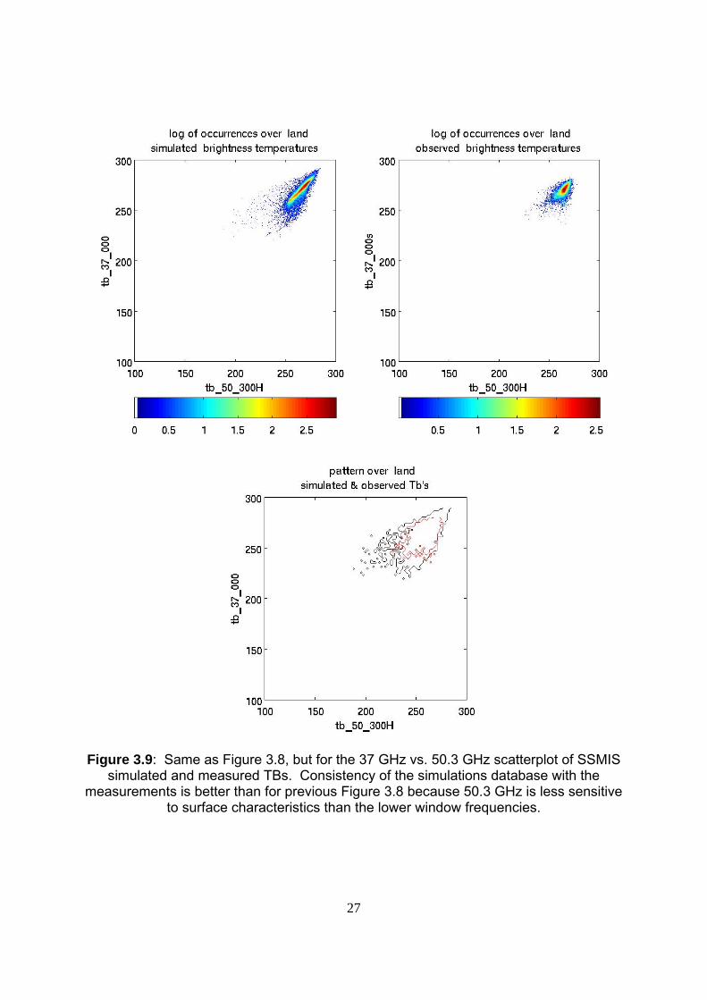
Figure 3.9: Same as Figure 3.8, but for the 37 GHz vs. 50.3 GHz scatterplot of SSMIS simulated and measured TBs. Consistency of the simulations database with the

measurements is better than for previous Figure 3.8 because 50.3 GHz is less sensitive to surface characteristics than the lower window frequencies.

28

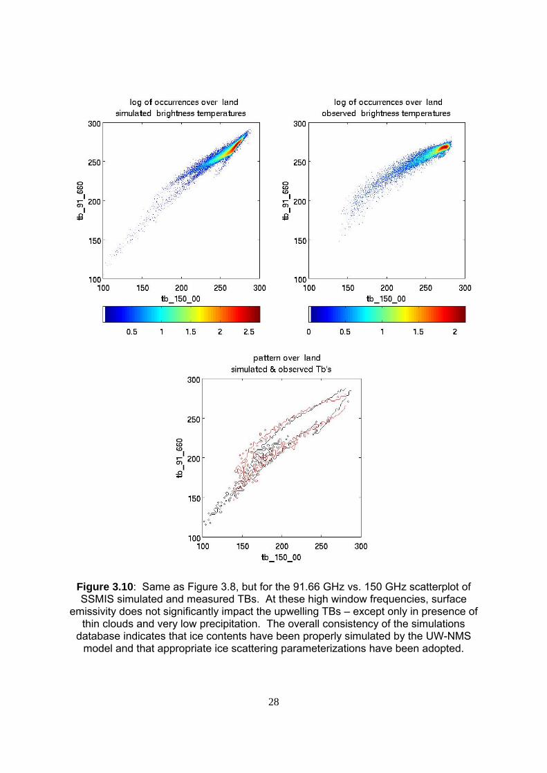
Figure 3.10: Same as Figure 3.8, but for the 91.66 GHz vs. 150 GHz scatterplot of SSMIS simulated and measured TBs. At these high window frequencies, surface

emissivity does not significantly impact the upwelling TBs – except only in presence of thin clouds and very low precipitation. The overall consistency of the simulations

database indicates that ice contents have been properly simulated by the UW-NMS model and that appropriate ice scattering parameterizations have been adopted.

29

Figure 3.11: Same as Figure 3.8, but for the 183.31±3 GHz vs. 183.31±7 GHz

scatterplot of SSMIS simulated and measured TBs. At these absorption frequencies of the intense water vapor line at 183.31 GHz, the impact of surface emissivity is always

negligible. As in Figure 3.10, the overall consistency of the simulations database indicates that ice contents have been properly simulated by the UW-NMS model and

that appropriate ice scattering parameterizations have been adopted – especially for the higher cloud portions.

30

3.2 An Application of the CDRD Algorithm We show here an application of the CDRD Algorithm using the European CRD / CDRD database developed for the H-SAF project. Specifically, we consider a case study over the Rome area, Italy, for which there are detailed ground validation measurements provided by the C-band polarimetric Doppler radar Polar 55C that is operated by the CNR-ISAC Radarmeteorology Group in Rome (see http://polar55c.artov.isac.cnr.it/). On July 2, 2009, a heavy storm hit the the Lazio region of central Italy, and particularly the area around the city of Rome. During the last days of June 2009, a cold pool descended from central Europe to the Balkans producing a cyclonic circulation over Eastern Europe. Consequently, an eastern flux developed over Italy carrying relatively cold air in the middle-level atmosphere. More in detail, a cold tongue at 850 mb developed over the Balkans on June 29, that generated, two days later, a strong cold advection over Italy. In addition, the summer solar irradiation triggered strong and diffuse convection along the Apennines mountain chain. As a result, thunderclouds were carried toward south-west by upper level winds – as shown in the Meteosat Second Generation (MSG) images of Figure 3.12.

Figure 3.12: High-Resolution-Visible (HRV) MSG images of the Italian region on 2 July 2009, 11:00 UTC (left) and 16:15 UTC (right), with superimposed contours of lightning

activity as detected by the ZEUS network during the previous 15 minutes. The red circle in the left panel indicates the Rome area observed by the CNR-ISAC Polar 55C radar.

Figure 3.13 shows the rainfall map over Rome area at 16:15 UTC, as measured by the Polar 55C radar. Figure 3.14 shows the brightness temperatures at 85 GHz, horizontal polarization, measured at 16:15 UTC by the SSM/I radiometer on board satellite DMSP F-15 of the of the U.S. Defense Meteorological Satellite Program (DMSP). In both figures, the heavy storm over the Rome area is quite evident.

31

Figure 3.13: Rainfall rates measured on 2 July 2009 at 16:15 UTC by the CNR-ISAC C-band polarimetric Doppler radar Polar 55C – note that the Rome area is represented by

the red circle.

Figure 3.14: Microwave brightness temperatures at 85 GHz, horizontal polarization, as measured by the SSM/I radiometer onboard the DMSP F-15 satellite on July 2, 2009,

16:15 UTC.

32

Figure 3.15 shows the corresponding retrieval results of our CDRD Algorithm, when applied in its CRD version (i.e., without dynamical tags). The most important features of these results are: a) heavy rain rates up to about 15 mm/hr are estimated over the Rome area; b) for each pixel, a large number of profiles from the European CRD database may be used by the Bayesian retrieval – and especially so for the low rain rates given their overwhelming number in the database; as a consequence, c) the retrieval uncertainty, as measured by the relative Bayesian variance, may be as large as the retrieved rain rate – thus, calling for a more constrained retrieval (such as in the CDRD approach).

Figure 3.15: Top panel: surface rain rates, RR (mm hr-1), obtained by the CDRD Algorithm in its CRD version from the upwelling TBs measured by the SSM/I radiometer

onboard DMSP F-15 satellite on 2 July 2009, 16:15 UTC. Bottom-left panel: corresponding number of profiles, np (logarithmic scale), from the European CRD

database that contributed, with their different Bayesian weights, to the Bayesian retrieval. Bottom-right panel: corresponding relative Bayesian variance, σ/RR (mm hr-1), of the retrieved surface rain rates (for each pixel, the Bayesian variance σ is computed from

the surface rain rates, with their different Bayesian weights, of all np profiles).

33

Figure 3.16 compares the satellite retrievals over the Rome area with the corresponding radar measurements of Figure 3.13 – note that to this end, we found it convenient to reduce radar measurements and satellite retrievals to a common resolution of about 50 km that was obtained by applying a 3x3 filter to the satellite retrievals. Evidently, there is a good agreement both in terms of precipitation path and rain rate values. Note, however, that while the fit of the scatterplot is close to the bisector, there is an high spread of the data.

Figure 3.16: Average (see text for more details) surface rain rates measured by the

Polar 55C radar (top left) and estimated by the CDRD Algorithm (top right) for the case study of 2 July 2009, 16:15 UTC. Bottom panel: scatterplot of satellite rainfall retrievals of top-right panel vs. corresponding radar measurements of top-left panel, with several

statistical indexes.

In order to check the performance of the CDRD version of our retrieval algorithm, we have performed the satellite retrievals for this case study using two dynamical tags (the Vertical Wind Velocity at 700 mb and the Near-surface Moisture Flux) in addition to the SSM/I TBs. Figure 3.17 shows the comparison with the radar data in a similar fashion than previous Figure 3.16. Obviously, the CDRD approach produces a better agreement with the radar measurements. This is especially evident by comparing the two satellite-radar scatterplots: the fit is now closer to the bisector and the spread of the data is significantly reduced. This improvement of the satellite retrieval by means of the CDRD approach is confirmed by the results of Figure 3.18, which shows that using

34

dynamical tags tends to increase the surface rain rates and decrease the Bayesian variance.

Figure 3.17: Same as Figure 3.16, but using the CDRD version of the satellite retrieval

algorithm (see text for more details).

Figure 3.18: Left panel: scatterplot of surface rain rates, RR (mm hr-1), estimated by the CRD version of the CDRD Algorithm vs. corresponding values estimated by the

CDRD version using two dynamical tag (see text for more details). Right panel: corresponding scatterplot of the relative Bayesian variances, σ/RR (mm hr-1).

35

4. SUMMARY AND CONCLUSIONS Within the H-SAF project – and particularly by means of its Visiting Scientist Programme –, we have generated a statistically significant Cloud-Radiation Database / Cloud Dynamics and Radiation Database for the European region to be used within the H-SAF project itself as an input to our physical-statistical profile-based Bayesian CDRD Algorithm for the retrieval of precipitation from conically-scanning microwave radiometers – H-SAF product PR-OBS-1. To this end, a large number (sixty) of simulations of different precipitation events over the European area for the March 2006 – February 2007 one-year period were performed by means of the cloud resolving model University of Wisconsin – Non-hydrostatic Modeling System, in such a way to take into account the various climatic regions, types of precipitation and seasonal variations. Then, an appropriate radiative transfer scheme was applied to the outputs of the UW-NMS simulations so as to simulate the upwelling brightness temperatures that would be measured by the conically-scanning SSM/I and SSMIS radiometers onboard DMSP satellites. As a result, about 300.000 different cloud structures at 15 km resolution, each containing at least one high-resolution (2 km) rainy profile, enter in the CRD / CDRD databases together with the associated upwelling TBs and the selected dynamical tags. In this Report, after discussing the CDRD approach and the generation of the European CRD / CDRD databases, we have presented some simple statistics for the microphysical properties of the cloud structures of the two databases, as well as for the simulated upwelling TBs for all relevant SSM/I – SSMIS channels. In both cases, we find large variations, which are due to the wide range of different meteorological and environmental conditions of the simulated events. Then, we have checked and discussed the “consistency” of the simulated TBs with the radiometric measurements from a large number of SSM/I and SSMIS overpasses over the European region. We find that in spite of all assumptions and uncertainties within the database generation procedure, the simulated TBs are generally consistent with the measured ones. We point out that this analysis has been useful to determine the most appropriate ice scattering parameterizations, as well as the weights of the various channels in the Bayesian retrieval procedure. Finally, we have shown an application of the algorithm using both the CRD and CDRD databases for a case study of heavy precipitation over the Rome area, Italy, for which there are detailed ground validation measurements provided by the CNR-ISAC C-band polarimetric Doppler radar Polar 55C. We find that there is a good agreement, both in terms of precipitation path and rain rate values, between the satellite retrievals using either the CRD or CDRD approach and the radar measuremens. We note, however, that the CDRD approach produces a better agreement by increasing the surface rain rates and decreasing the Bayesian variance. During Summer 2009, the CRD version of the CDRD Algorithm has been made available, together with the CRD database, to the H-SAF project and is now participating to the H-SAF Ground Validation and Hydrological Validation Activities. The full CDRD Algorithm will be made available during the first period of H-SAF Continuous

36

Development and Operations Phase (CDOP-1) that has been recently proposed to EUMETSAT for the September 2010 – February 2012 time frame. The CDRD approach has been presented since 2006 at several International meetings and conferences (e.g., Mugnai et al., 2006). We are now preparing two manuscripts on the CDRD approach (Smith et al., 2010) and on its application to a series of precipitation events (Sanò et al., 2010), that will be submitted soon to the Natural Hazards and Earth System Sciences (NHESS) journal of the European Geosciences Union (EGU) for publication on a special issue dedicated to the 11th EGU Plinius Conference on Mediterranean Storms, that was held last September in Barcelona, Spain.

37

5. REFERENCES Bauer, P., L. Schanz and L. Roberti, 1998: Correction of the three-dimensional effects

for passive microwave remote sensing of convective clouds. J. Appl. Meteor., 37, 1619-1632.

Bohren, C.F., and D.R. Huffman, 1983: Absorption and Scattering of Light by Smal particles. John Wiley & Sons, 530 pp.

Cotton, W.R., G.J. Tripoli, R.M. Rauber and E.A. Mulvihill, 1986: Numerical simulation of the effects of varying ice crystal nucleation rate and aggregation processes on orographic snowfall. J. Clim. Apl. Meteor. 25: 1658-1680.

Czekala, H., P. Bauer, D. Jones, F. Marzano, A. Tassa, L. Roberti, S. English, J.P.V. Poiares Baptista, A. Mugnai and C. Simmer, 2000: Clouds and Precipitation. Radiative Transfer Models for Microwave Radiometry (C. Matzler, Ed.), COST Action 712, Directorate-General for Research, European Commission, Brussels, Belgium, 37-72.

Di Michele S., A. Tassa, A. Mugnai, F.S. Marzano, P. Bauer and J.P.V. Poiares Baptista, 2005: The Bayesian Algorithm for Microwave-based Precipitation Retrieval: Description and application to TMI measurements over ocean. IEEE Trans. Geosci. Remote Sens., 43, 778-791.

Di Michele S., F.S. Marzano, A. Mugnai, A. Tassa and J.P.V. Poiares Baptista, 2003: Physically-based statistical integration of TRMM microwave measurements for precipitation profiling. Radio Sci., 38, 8072-8088.

English, S.J., and T.J. Hewison, 1998: A fast generic millimetre wave emissivity model. Proc. SPIE on Microwave Remote Sensing of the Atmosphere and Environment, 22-30.

Flatau P., G.J. Tripoli, J. Berlinde and W. Cotton, 1989: The CSU RAMS Cloud Microphysics Module: General Theory and Code Documentation. Technical Report 451, Colorado State University, 88 pp.

Grenfell, T.C., and S.G. Warren, 1999: Representation of a nonspherical ice particle by a collection of independent spheres for scattering and absorption of radiation. J. Geophys. Res., 104, 31697-31709.

Hewison, T.J., and S.J. English, 1999: Airborne retrievals of snow and ice surface emissivity at millimetre wavelengths. IEEE Trans. Geosci. Remote Sens., 37, 1871-1879.

Hewison, T.J., and S.J. English, 2000: Fast models for land surface emissivity. Radiative Transfer Models for Microwave Radiometry (C. Matzler, Ed.), COST Action 712, Directorate- General for Research, European Commission, Brussels, Belgium, 117-127.

Hewison, T.J., 2001: Airborne measurements of forest and agricultural land surface emissivity at millimeter wavelengths. IEEE Trans. Geosci. Remote Sens., 39, 393-400.

Heymsfield, A.J., and L. M. Miloshevich, 2003: Parameterizations for the cross-sectional area and extinction of cirrus and stratiform ice cloud particles. J. Atmos. Sci., 60, 936-956.

38

Kummerow, C.D., 1993: On the accuracy of the Eddington-approximation for the radiative transfer in microwave frequencies. J. Geophys. Res., 98, 2757–2765.

Liu, G., C. Simmer and E. Ruprecht, 1996: Three-dimensional radiative transfer effects of clouds in the microwave spectral range. J. Geophys. Res., 101, 4289-4298.

Mugnai, A., F. Baordo, J. Hoch, C.M. Medaglia, A. Metha, E.A. Smith and G.J. Tripoli, 2006: Precipitation retrieval and analysis of severe storm events based on Cloud Dynamics and Radiation Database (CDRD) approach. Geophysical Research Abstracts, Volume 8, ISSN:1029-7006, EGU General Assembly 2006, Vienna, Austria, 2-7 April 2006.

Mugnai, A., S. Di Michele, F.S. Marzano and A. Tassa, 2001: Cloud-model based Bayesian techniques for precipitation profile retrieval from TRMM microwave sensors. ECMWF/EuroTRMM Workshop on Assimilation of Clouds and Precipitation, ECMWF, Reading, U.K., 323-345.

Neshyba, S.P., T.C. Grenfell and S.G. Warren, 2003: Representation of a nonspherical ice particle by a collection of independent spheres for scattering and absorption of radiation: 2. Hexagonal columns and plates. J. Geophys. Res., 108, 4448-4465.

Olson, W.S., P. Bauer, N.F. Viltard, D.E. Johnson, W.K. Tao, R. Meneghini and L. Liao, 2001: A melting layer model for passive/active microwave remote sensing applications. Part II: Simulation of TRMM observations. J. Appl. Meteor., 40, 1164-1179.

Panegrossi, G., S. Dietrich, F.S. Marzano, A. Mugnai, E.A. Smith, X. Xiang, G.J. Tripoli, P.K. Wang and J.P.V. Poiares Baptista, 1998: Use of cloud model microphysics for passive microwave-based precipitation retrieval: Significance of consistency between model and measurement manifolds. J. Atmos. Sci., 55, 1644-1673.

Roberti, L., J. Haferman and C. Kummerow, 1994: Microwave radiative transfer through horizontally inhomogeneous precipitating clouds. J. Geophys. Res., 99, 707-716.

Sanò, P., D. Casella, S. Dietrich, F. Di Paola, M. Formenton, W.-Y. Leung, A. Mehta, A. Mugnai, E.A. Smith and G.J. Tripoli, 2010: Bayesian estimation of precipitation from space using the Cloud Dynamics and Radiation Database (CDRD) approach: Application to case studies of FLASH and H-SAF Projects. Nat. Hazards Earth Syst. Sci., to be submitted.

Schluessel, P.; and H. Luthardt, 1998: Surface wind speeds over the North Sea from Special Sensor Microwave/Imager observations. J. Geophys. Res., 96, 4845–4853.

Smith, E.A., A. Mugnai and G.J. Tripoli, 2010: A new paradigm for satellite retrieval of hydrologic variables: The CDRD methodology. Nat. Hazards Earth Syst. Sci., to be submitted.

Surussavadee, C., 2006: Passive millimeter-wave retrieval of global precipitation utilizing satellites and a numerical weather prediction model. Ph.D. dissertation, Dept. Elect. Eng. and Comput. Sci., MIT, Cambridge, MA.

Tassa, A., S. Di Michele, A. Mugnai, F.S. Marzano, P. Bauer and J.P.V. Poiares Baptista, 2006: Modeling uncertainties for passive microwave precipitation retrieval: Evaluation of a case study. IEEE Trans. Geosci Remote Sens., 44, 78-89.

39

Tassa, A., S. Di Michele, A. Mugnai, FS. Marzano and J.P.V. Poiares Baptista, 2003: Cloud-model based Bayesian technique for precipitation profile retrieval from the Tropical Rainfall Measuring Mission Microwave Imager. Radio Sci., 38, 8074-8086.

Tripoli G.J. and E.A. Smith, 2009: Scalable nonhydrostatic cloud/mesoscale model featuring variable-stepped topography coordinates: Formulation and performance on classic obstacle flow problems. Mon. Wea. Rev., submitted.

Tripoli, G.J., and W.R. Cotton, 1981: The use of ice-liquid water potential temperature as a thermodynamic variable in deep atmospheric models. Mon. Wea. Rev., 109, 1094-1102.

Tripoli, G.J., 1992: A nonhydrostatic model designed to simulate scale interaction. Mon. Wea. Rev., 120, 1342-1359.

Wiscombe, W.J., 1980: Improved Mie scattering algorithms. Appl. Opt., 19, 1505-1509.