Sampling design optimization for spatial functions of observation...Mathematical Geology, Vol. 16, No. 4, 1984 Sampling Design Optimization for Spatial Functions Ricardo A. Oiea 2

Mathematical Geology, Vol. 16, No. 4, 1984

Sampling Design Optimization for Spatial Functions

R i c a r d o A. Oiea 2

A new procedure is presented for minimizing the sampling requirements necessary to estimate a mappable spatial function at a specified level o f accuracy. The technique is based on universal kriging, an estimation method within the theory o f regionalized variables. Neither actual implementation o f the sampling nor universal kriging estimations are necessary to make an optimal design. The average standard error and maximum standard error of estimation over the sampling domain are used as global indices o f sampling efficiency. The procedure optimally selects those parameters controlling the magnitude o f the indices, including the density and spatial pattern o f the sample elements and the number o f nearest sample elements used in the estimation. As an illustration, the network o f observation wells used to monitor the water table in the Equus Beds o f Kansas is analyzed and an improved sampling pattern suggested. This example demonstrates the practical utility o f the procedure, which can be applied equally well to other spatial sampling problems, as the procedure is not limited by the nature o f the spatial function.

KEY WORKS: spatial funetion, sampling, sample element, universal kriging, standard error, contour mapping.

INTRODUCTION

A spatial function is an association of numbers to a domain of geographic coor- dinates. Spatial functions may be one dimensional, such as a petrophysical well log, two dimensional, such as a contour map, or three dimensional, such as the variation in grade of ore within a mine. Spatial functions are continuous and uniquely defined over sizeable domains. Although fluctuations may be erratic and unpredictable in detail from one location to another, usually an underlying trend in the fluctuations precludes regarding the variable as completely random. Typically, observations which are closely spaced are autocorrelated.

Some spatial functions, for example, geothermal gradients, are not easily measured and their accurate characterization presents an expensive and time- consuming problem. Most spatial functions of a geologic nature can be known

1Manuscript received 15 November 1982; revised 31 May 1983. eKansas Geological Survey, 1930 Avenue A, Lawrence, Kansas 66044 U.S.A. Present ad-

dress: Empresa Nacional del Petr61eo, Casilla 3556, Santiago, Chile. 369

0020-5958/84/0500-0369503.50/0 © 1984 Plenum Publishing Corporation

370 Olea

only partially through scattered sets of expensively gathered measurements. Ob- servations of a spatial function constitute a statistical sample. However, because spatial functions possess continuity and each location is unique, classical statistical theory and sampling procedures are not applicable. Rather, we must turn to a special statistical theory which explicitly considers spatial properties, the theory of regionalized variables.

Although regionalized variable theory has been extensively described in the geomathematical and statistical literature, almost all discussions focus on either the problem of estimation or on simulation, while only a few studies have marginally addressed the question of the efficient arrangement of the sample elements (Alldredge and Alldredge, 1978; Ripley, 1981, p. 214-241). This paper treats the specific problem of sampling mappable geologic properties, the large class of regionalized variables whose observations can be regarded as points in two-dimensional space.

OPTIMUM SAMPLING

Estimation Method

The estimation method selected for this study is universal kriging, an unbiased linear estimator with minimum estimation variance properties, based upon the theory of regionalized variables (Matheron, 1971 ; Olea, 1975). Region- alized variable theory is a set of statistical principles which mathematically considers spatial function properties but which neglects the physical nature of the phenomenon under study. This makes the theory extremely general and accounts for its great range of applicability (Matheron, 1965; Journel and Huijbregts, 1978).

Regionatized variable theory uses random variables to model spatial functions. The standard deviation of an unbiased estimator of a random variable is the standard error (James and James, 1976). Since the standard error is given in the same units as the estimated value itself, it is useful as a measure of uncertainty in the estimate. A basic reason for selecting universal kriging is because it is a well-established estimation method for spatial functions that provides the standard error of the estimate.

Measures of Sampling Performance

The global performance of samples over the sampling domain of a spatial function can be judged by two indices: the average standard error and the maximum standard error. These measures depend upon:

1. Unmanageable factors a. The semivariance b. The drift

Sampling Optimization for Spatial Functions 371

2. Manageable factors a. The size of the sample subset of nearest neighbors considered by the

estimate b. The sample pattern c. The sample density

Of the factors that influence the sampling efficiency indices, two have nothing to do with sampling and a third is only partially related to sampling. The semivariance and drift are inherent in the spatial function. The investi- gator designing a sampling program is limited to selecting models that provide the best fits to the true semivariogram and the drift. Specification of the size of the sample subset used in universal kriging calculations is primarily a problem in computational efficiency, with some sampling implications. This leaves sample pattern and sample density as the only two factors offering wide flexibility in the design of the sampling scheme.

Sensitivity Analysis

The semivariance of a regionalized variable depends upon the drift, and vice versa, but all other factors are independent from one another (Olea, in prep.). This analysis is restricted to a consideration of a linear model through the origin for the semivariance and polynomial models up to degree two for the drift. These restrictions result from the decision to develop a general procedure that is suf- ficiently simple to be applied to a wide variety of sampling and mapping problems.

"Pattern" refers to the geometrical configuration of the sample elements in space. Unfortunately, pattern is a nominal characteristic of discrete categories which have no implicit order. A distance index and the maximum number of symmetry axes through a point were computed for several configurations of sample points. The distance index of a set of points in two-dimensional space is defined as the ratio of the average distance to each observed nearest neighbor, over the average distance to a nearest neighbor in a random set of points (Clark and Evans, 1954). The arrangement of the 12 patterns shown in Fig. 1 indicates that those selected for analysis cover the spectrum of possibilities.

As pattern is a nominal variable and the size of the sample subset considered is an integer variable, the sampling efficiency indices are not continuously defined. Only the third factor, sample density, can be expressed as a continuous variable. A function of three variables is difficult tO represent graphically; standard practice is to set one variable to a selected value and to present the family of surfaces defined by the other two variables. Since pattern is by nature discrete, it was selected as the parameter to be held constant. For ease of presenta- tion, the number of nearest neighbors is shown as a continuous variable. Figure 2 is an example, diagrammatically representing the average standard error for two patterns.

372 Olea

2.0

1.6

--=1.2

._~

0.8

-~.. '..... ® , . ' . . . %

.( ; ; . . ,...

® :: £2727

2::::::{::::

. . . . . . I

• :, } ' : ' ' : . ®

. . . , - - - . . ,

, . . % , . . . .

( ' . . . . ® ~ i @

. : " 4 i " ' . . : . . . " '" ' . @ : . , . . ' . / ' - , - . < . . . . . . . . : . . . .

7 " ' " ' 7" "'." , . . . . , . • . . . .

. , . . . 4 . , , , . .

0.4 ~ ® , , @

¢:

= i @ . . . .

O

0 2 4 6 Maximum Number Of Symmetry Axes Through A Point

Fig. 1. Two-dimensional point patterns at a fixed density. (t) Hexagonal; (2) square; (3) triangular; (4) and (8) orthogonal traverses; (5) stratified hexagonal; (6) random; (7) and (10) bisymmetric; (9) and (12) clustered; (11) regular cluster.

The following assertions are given here without proof. Extensive discussion of these points, with formal proofs where appropriate, are given by Olea (in prep.).

1. The square of the standard error varies linearly with the slope of the semivariogram. The effect of semivariogram slope can be analyzed independently of other factors.

2. If all other factors are the same, significant differences in the indices will result from different sampling patterns, summarized in Table 1. The absence of units for standard error in tables in this report is intended to emphasize the


O

C r~

~2

J J

J

\ !°

0 / / I O / f

/ . / / /

/ /

/ / ~,a@

(Density)-2

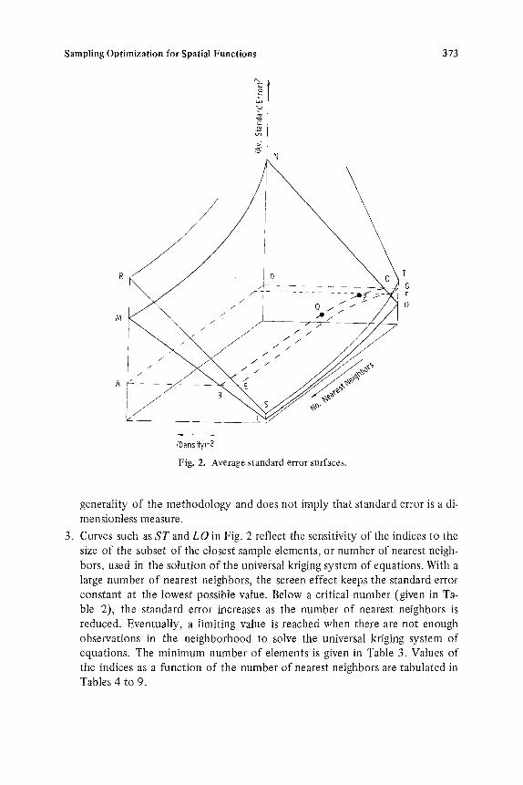
Fig. 2. Average standard error surfaces.

generality of the methodology and does not imply that standard error is a di- mensionless measure.

3. Curves such as ST and LO in Fig. 2 reflect the sensitivity of the indices to the size of the subset of the closest sample elements, or number of nearest neighbors, used in the solution of the universal kriging system of equations. With a large number of nearest neighbors, the screen effect keeps the standard error constant at the lowest possible value. Below a critical number (given in Ta- ble 2), the standard error hlcreases as the number of nearest neighbors is reduced. Eventually, a limiting value is reached when there are not enough observations in the neighborhood to solve the universal kriging system of equations. The minimum number of elements is given in Table 3. Values of the indices as a function of the number of nearest neighbors are tabulated in Tables 4 to 9.

374 Olea

Table 1. Sensitivity of the Sampling Efficiency Indices to Pattern, Assuming Unit Density, Unit Linear Semivariogram Slope, and 32 Nearest Neighbors a

Average standard Maximum standard error drift error drift

Distance Symmetry Pattern index axes 0 1 2 0 1 2

Hexagonal(i) 2.15 6 0.63 0.63 0.63 0.72 0.72 0.72 Square (2) 2.00 4 0.64 0.64 0.64 0.74 0.74 0.74 Triangular (3) 1.75 6 0.66 0.66 0.66 0.80 0.80 0.80 Traverses every

two points (4) 1.41 4 0.68 0.68 0.68 0.89 0.89 0.89 Hexagonal strati-

fication (5) 1.26 - 0.69 0.69 0.69 0.86 0.86 0.86 Random (6) 0.91 - 0.71 0 .71 0.71 1.05 1.05 1.05 Bisymmetrical

random(7) 0.82 2 0.72 0.72 0.72 0.98 0.98 0.98 Traverses every

eight points (8) 0.92 4 0.81 0 .81 0.84 1.23 1.23 1.45 Five clusters (9) 0.34 - 0.98 0.99 1.06 1.33 1.49 2.33 Bisymmetrical

clusters(10) 0.33 2 1.03 1 .03 1.11 1.22 1.22 1.38 Sixteen points

per regular cluster (11) 0.40 4 1.13 1 .17 1.53 1.51 1.85 5.13

One cluster(12) 0.13 - 2.19 5.01 61.50 2.94 8.27 148.00

aNurnbers in parentheses correspond to the pattern identification number in Fig. 1.

. Sampling efficiency indices vary with the fourth root of the pattern density p

2V I(1, 1)3 4 (1)

where co is the slope of the linear semivariogram; I(1, 1) is the efficiency in-

dex in Table 1 for the given pattern at a density of one point per square mile (0.39 points/kin 2) and a semivariogram slope of 1 ; and I(co, P) is the level

specified for the sampling efficiency index. Equation 1 is a new formula that expresses the interrelation of each of the sampling efficiency factors, as these factors are not explicit in the general estimation variance formulas. In addi- tion, eq. 1 deals with global rather than point estimates of estimation variance.

A Systematic Approach to Sampling

A trivial solution to the sampling problem is to select an infinite density of points, insuring efficiency indices equal to zero. When continuous sampling is not feasible, seeking the best sampling procedure becomes an operations re-


Table 2. Minimum Number of Sample Elements Required to Obtain Constant Values for the Sampling Efficiency Indices

Average standard Maximum standard error drift error drift

Pattern 0 1 2 0 1 2

Hexagonal 3 5 10 3 5 10 Square 4 5 10 10 10 14 Triangular 8 8 11 11 12 12 Traverses every two points 12 12 20 14 15 26 Hexagonal stratification 6 6 16 7 8 25 Random 12 12 32+ 12 14 32+ Bisymmetrical random 8 8 32+ 20 28 32+ Traverses every eight points 28 32+ 32+ 28 32+ 32+ Five clusters 32+ 32+ 32+ 32+ 32+ 32+ Bisymmetrical clusters 20 20 32+ 26 28 32+ Sixteen points per regular

cluster 32+ 32+ 32+ 32+ 32+ 32+ One cluster 32+ 32+ 32+ 32+ 32+ 32+

Table 3. Minimum Number of Sample Elements Required to Solve the Universal Kriging System of Equations

Drift

Pattern 0 1 2

Hexagonal 1 3 6 Square 1 3 7 Triangular 1 3 7 Traverses every two points 1 3 9 Hexagonal stratification 1 3 6 Random 1 '3 6 Bisymmetrical random 1 3 9 Traverses every eight points 1 5 9 Five clusters t 3 6 Bisymmetrical clusters 1 5 12 Sixteen points per regular

cluster 1 5 9 One cluster 1 3 7

search problem: For a given sampling eff ic iency index level, minimize the sam-

pling requirements . Specif icat ion o f the level o f the sampling eff ic iency index is

external to the sampling p rob lem itself. The sampling eff ic iency index levels

should be de termined according to such requi rements as economics of data col-

lect ion, fur ther uses o f the col lected informat ion , and the acceptable level o f uncer ta in ty .

376 Olea

Table 4. Average Standard Error When the Drift is a Constant, Assuming Unit Density and Unit Semivariogram Slope

Number of nearest neighbors

Pattern 1 2 3 4 6 8 12 16 32

Hexagonal Square Triangular Orthogonal traverses

every two points Hexagonal stratification Random Bisymmetrical random Orthogonal traverses

every eight points Five clusters Bisymmetrical clusters Sixteen points per

regular cluster One cluster

0.83 0.67 0.63 0.63 0.63 0.63 0.63 0.63 0.63 0.86 0.68 0.65 0.64 0.64 0.64 0.64 0.64 0.64 0.88 0.74 0.69 0.68 0.67 0.66 0.66 0.66 0.66

0.92 0.78 0.73 0.71 0.70 0.69 0.69 0.68 0.68 0.90 0.76 0.72 0.70 0.69 0.69 0.69 0.69 0.69 0.93 0.82 0.78 0.76 0.73 0.72 0.72 0.71 0.71 0.95 0.82 0.78 0.75 0.73 0.72 0.72 0.72 0.72

1.08 0.99 0.95 0.93 0.88 0.86 0.84 0.83 0.81 1.27 1.21 1.17 1.14 1.12 1.08 1.05 1.03 0.98 1.37 1.30 1.28 1.27 1.20 1.19 1.06 1.04 1.03

1.49 1.39 1.37 1.36 1.35 1.32 1.27 1.24 1.13 2.26 2.25 2.24 2.23 2,22 2.22 2.20 2.20 2.19

Table 5. Average Standard Error Assuming First-Degree Polynomial Drift, Unit Density, and Unit Semivariogram Slope


Pattern 3 4 5 6 8 12 16 32

Hexagonal Square Triangular Orthogonal traverses

every two points 1.02 0.77 Hexagonal stratification 1.47 0.74 Random 1.91 0.96 Bisymmetrical random 21.92 0.84 Orthogonal traverses

every eight points - - Five clusters 3.69 2.71 Bisymmetrical clusters - - Sixteen points per

regular cluster - - One cluster 148.00 33.87

0.65 0.64 0.63 0,63 0.63 0.63 0.63 0.63 0.66 0.65 0.64 0.64 0.64 0.64 0.64 0.64 0.80 0.69 0.67 0,67 0.66 0.66 0.66 0.66

0.72 0.70 0.69 0.69 0.68 0.68 0.70 0.69 0.69 0.69 0.69 0.69 0.82 0.77 0.73 0.72 0.71 0.71 0.77 0.74 0.72 0.72 0.72 0.72

1.24 1.14 1.02 0.88 0.83 0.81 2.20 1.98 1.60 1.33 1.18 0.99 2.50 2.24 1.93 1.18 1.07 1.03

2.96 2.75 2.29 1.83 1.62 1.17 19.74 13.92 9.17 7.15 6.31 5.01

Sampling Opt imizat ion for Spatial Funct ions 377

Table 6. Average Standard Error Assuming Second-Degree Polynomial Drift, Unit Density, and Unit Linear Semivariogram Slope


Pat tern 6 7 8 9 12 16 32

Hexagonal 0.68 0.67 0.66 0.65 0.63 0.63 0.63 Square - 0.67 0.67 0.66 0.64 0.64 0.64 Triangular - 0.77 0.72 0.69 0.66 0.66 0.66 Orthogonal traverses

every two points - - - 0.76 0.71 0.69 0.68 Hexagonal stratification 1.55 0.86 0.77 0.74 0.70 0.69 0.69 Random 26.71 1.42 1.06 0.88 0.77 0.74 0.71 Bisymmetr ica random - - - 0.85 0.76 0.73 0.72 Orthogonal traverses

every eight points - - - 1.69 1.30 1.16 0.84 Five clusters 88.99 17.76 12.80 9.68 4.90 2.71 1.07 Bisymmetrical r andom - - - - 9.92 1.62 1.I1 Sixteen points per

regular cluster - - 12.94 7.25 4.78 1.53 One cluster - 2214.00 936.00 547.00 275.00 171.00 61.50

Table 7. Maximum Standard Error When the Drift is a Constant , Assuming Unit Density and Unit Linear Semivariogram Slope


Pat tern 1 2 3 4 6 8 12 16 32

Hexagonal 1.11 0.84 0.72 0.72 0.72 0.72 0.72 0.72 0.72 Square 1.19 0.88 0.80 0.75 0.75 0.75 0.74 0.74 0.74 Triangular 1.32 1.14 0.98 0.88 0.81 0.81 0.80 0.80 0.80 Orthogonal traverses

every two points 1.50 1.27 1.14 1.05 0.93 0.91 0.90 0.89 0.89 Hexagonal stratification 1.30 1.07 1.02 0.94 0.87 0.86 0.86 0.86 0.86 Random 1.48 1.34 1.34 1.23 1.16 1.06 1.06 1.05 1.05 Bisymmetrical random 1.60 1.45 1.33 1.32 1.05 1.00 0.99 0.99 0.98 Orthogonal traverses

every eight points 2.01 1.94 1.80 1.76 1.31 1.39 1.29 1.24 1.23 Five clusters 1.83 1.82 1.75 1.74 1.70 1.67 1.64 1.46 1.33 Bisymmetrical clusters 1.92 1.83 1.83 1.83 1.76 1.76 1.40 1.39 1.22 Sixteen points per

regular cluster 2.19 2.06 2.06 2.05 2.05 1.90 1.90 1.74 1.51 One cluster 2.99 2.98 2.98 2.98 2.97 2.96 2.96 2.95 2.94

378 Olea

Table 8. Maximum Standard Error Assuming First-Degree Polynomial Drift, Unit Density, and Unit Semivariogram Slope


Pattern 3 4 5 6 8 12 16 32

Hexagonal 0.73 0.73 0.72 0.72 0.72 0.72 0.72 0.72 Square 0.84 0.75 0.75 0.75 0.75 0.74 0.74 0.74 Triangular 1.47 0.93 0.83 0.81 0.81 0.80 0.80 0.80 Orthogonal traverses

every two points 2.45 1.40 1.02 0.94 0.91 0.90 0.89 0.89 Hexagonal stratification 15.39 1.30 0.89 0 1 8 7 0.86 0.86 0.86 0.86 Random 19.74 3.26 1.84 1.58 1.11 1.06 1.05 1.05 Bisymmetrical random 307.00 3.02 1.36 1.14 1.00 0.99 0.99 0.98 Orthogonal traverses

every eight points - - 2.58 2.21 1.77 1.45 1.25 1.23 Five clusters 12.35 11.76 5.33 5.23 4.24 3.26 2.28 1.49 Bisymmetfical clusters - - 6.04 5.12 4.22 2.26 1.98 1.22 Sixteen points per

regular cluster - - 5.80 5.48 4.17 3.72 2.90 1.85 One cluster 793.00 118.00 98.19 46.45 18.47 12.55 10.13 8.27

Table 9. Maximum Standard Error Assuming Second-Degree Polynomial Drift, Unit Density, and Unit Linear Semivariograrn Slope


Pattern 6 7 8 9 12 16 32

Hexagonal 0.78 0.76 0.76 Square - 0.79 0.78 Triangular - 1.07 0.99 Orthogonal traverses

every two points - - - Hexagonal

stratification 39.91 1.57 1.14 Random 2690.00 11.60 7.90 Bisymmetrical

random - - - Orthogonal traverses

every eight points - - - Five clusters 986.00 142.00 101.00 Bisymmetrical

clusters - - - Sixteen points per

regular cluster - - - One cluster

0.74 0.72 0.72 0.72 0.77 0.75 0.74 0.74 0.87 0.80 0.80 0.80

1.27 0.97 0.90 0.89

1.07 0.90 0.87 0.86 2.03 1.32 1.15 1.05

1.96 1.25 1.07 0.98

8.84 4.48 3.27 1.45 101.00 32.87 12.30 2.33

- 107.00 10.03 1.38

33.47 23.71 12.10 5.13 10425.00 8763.00 1956.00 815.00 535.00 148.00


Let us assume that the desired average standard error is D in Fig. 2. A hori- zontal plane through D intersects the average standard error surfaces along lines BQPC and EF. Points along arc QPC on the lowest surface will provide the required average standard error. A solution such as P requires the minimum number of nearest neighbors for a given density. Given a density, no other pattern requires fewer nearest neighbors to produce the specified average standard error. Should LMNO be the surface corresponding to a hexagonal pattern of sampling points, the optimum found would be an absolute optimum. Otherwise, the curve QPC is an optimum solution relative to the subset of feasible sampling patterns.

This graphic solution to the sampling problem can be organized as a systematic procedure which will yield an optimal solution if one is feasible. Due to the assumptions made in the analysis, the procedure is subject to the following constraints: (a) the residuals satisfy the intrinsic hypothesis; (b) the physical size of the support of the sample elements and the estimated value are the same; (c) the sampling space is two dimensional; (d) the semivariogram of the residuals is linear, isotropic, and without nugget effect.

Constraint (b) is the strongest and excludes certain spatial functions which are of interest in ore reserve estimation. Constraint (c) is satisfied in all mapping problems. Even in studies of three-dimensional space, samples may be collected in a series of two-dimensional planes, which helps to satisfy the constraint (b). The semivariance is a monotonically increasing function close to the origin. Be- cause even complex functions can be approximated by linear piecewise inter- polation procedures, the problem of satisfying constraint (d) becomes one of determining how large a portion of the semivariogram can be approximated by a single straight line. The shape of the semivariogram beyond the range is imma- terial if the nearest neighbors in the subset used in the estimations are all statis- tically correlated; that is, if their relative distances are never larger than the range.

Algorithm 1

The following is a procedure for finding the optimal sampling design for a specified sampling efficiency index.

1. Perform a structural analysis.

2. Decide whether the average standard error or the maximum standard error is the deciding criterion.

3. Enter Table 1 for the specified index and appropriate drift. Choose the pattern with the lowest index in the table. In case of a tie, use the pattern with the minimum alternative index.

4. Specify a value for the sampling efficiency index.

5. Use eq. 1 to compute the required density using the minimum index of step 2.

380 Olea

6. Calculate the number of sample elements within the neighborhood for which the models in the structural analysis are valid.

7. Compare the number of sample elements inside the neighborhood with the minimum number of points necessary to achieve a solution of the universal kriging system of equations in Table 3. Should the number of points inside the neighborhood be insufficient, the solution is unfeasible. In case a solution is required, go back to step 1 and redefine parameters. Otherwise, stop. If there are enough sample elements inside the neighborhood, proceed to the next step.

8. Enter Table 2 and determine the minimum number of sample elements required to obtain constant values for the index, which is the point of no return.

9. Compare the sample elements inside the neighborhood to the point of no return. In case the point of no return is smaller than the number of points that can be placed inside the neighborhood, use a number of nearest neighbors equal to the point of no return and stop. Otherwise, use a number of nearest neighbors equal to the number of points inside the neighborhood.

10. Find in Tables 4 through 9 the selected index and appropriate drift. Take the pattern that minimizes the index for the number of nearest neighbors computed in the previous step.

11. Enter the minimum index selected on the preceding step into eq. 1 to re- compute the optimal density. Stop.

The procedure requires a priori knowledge of the spatial characteristics of the function as provided by structural analysis. But notice that neither actual implementation of the sampling procedure nor universal kriging estimations are necessary. The algorithm will provide a sampling design through the use of a few simple calculations and the tables.

CASE STUDY

The inadequacies of a haphazardly developed sampling pattern are illus- trated by the network used to monitor the water table elevation in the Equus Beds aquifer of central Kansas (Fig. 3). As a demonstration of the economic and scientific advantages of a rationally designed sampling scheme, an optimized alternative observation network is presented.

The Equus Beds

The Equus Beds aquifer produces groundwater through more than 2000 in- dustrial, municipal, and irrigation wells in Harvey, Sedgwick, McPherson, and Reno counties in south-central Kansas. The Equus Beds are stream-laid deposits of the Pliocene Blanco and the Pleistocene Meade and Sanborn formations


b- ÷

I/ ,A

';i iiiilil ii iiii i

] SEDGWICK 0 10 l i

I miles

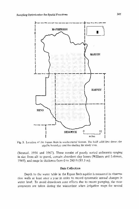
Fig. 3. Location of the Equus Beds in south-central Kansas. The bold solid line shows the aquifer boundary and the shading the study area.

(Stramel, 1956 and 1967). These consist of poorly sorted sediments ranging in size from silt to gravel, contain abundant clay lenses (Williams and Lohman, 1949), and range in thickness from 0 to 280 ft (85.3 m).

Data Collection

Depth to the water table in the Equus Beds aquifer is measured in observation wells at least once a year in order to record systematic annual changes in water level. To avoid drawdown cone effects due to recent pumping, the measurements are taken during the wintertime when irrigation stops for several

382 Olea

Fig. 4. Water-table elevation in the Equus Beds as perceived by the present network of 244 wells. Locations of observation wells are shown by crosses.

months. Data used were the latest available at the outset of the study and consist of measurements made from December 1980 to March 1981. The measure-

ments used here are only a fraction of a statewide survey (Olea, 1982). Figure 4 is a contour map of the water table in the Equus Beds, based on these data. Fig- ure 5 is the corresponding standard error map, and Fig. 6 is a histogram showing the relative frequency of the standard errors of the water table in Fig. 5.


130- ? z! ÷ D ÷ + ¢ + + . + ~ 4- 4-

4- 4- 4-4- + 4- 4- + */ 4- 4- 4 - ; + ~ 4- + 4 - * 4- 4- h

4- 4- +++ , 4 - * * + . , 4-4- 4-+ 4- 4- 4- 4- + t +

+ ~+ + 4-~- + + + + 4-+ ~ t + 4- l 4- + 4- +

A 4- / ~ 4- 4-4- 4- ~4-+# 4- 4-4- "<9_J f + + + ~ , + + + +4-+ + -~-~-+~+* +

4- ++e ~: +

~ , + +

'0 5 + + +

I N + 0 + m i l e s +

Fig. 5. Standard error of the water-table elevation in the Equus Beds as perceived by the present network of 244 wells. Locations of observation wells are shown by crosses.

Critical Analysis

The present observat ion n e t w o r k i n t h e Equus Beds has deficiencies be-

cause observa t ion wells have been added to the n e t w o rk in a haphazard fashion

over t ime. We first note tha t the sampling pa t t e rn is no t opt imal . As the Equus

Beds n e t w o r k includes 244 observa t ion wells in an area o f 800 square miles

384

25

Olea

2O

E i -

. 15

c

g 10

5

0 0 I0 20 30

Slandard Error, Ft.

Fig. 6. Relative frequency of the standard error of the water-table elevation in the Equus Beds as perceived by the present network of 244 wells. The mean is 9.98 ft and the standard deviation is 4.77 ft.

(2071 km2), the sampling density is 0.305 wells per square mile (0.12 wells/km2). Since the average nearest-neighbor distance between wells is 0.91 miles (1.46 km), the distance index is 1.0. Overall, the pattern of wells in the network is indistinguishable from a random arrangement (Clark and Evansl 1954). Random patterns do not compare favorably to other patterns in terms of their sampling efficiency indices (see Table 1). Observation wells arranged in a regular pattern, in stratified patterns, or along closely spaced profiles would produce equivalent results more efficiently than the present network.

We also note that sampling density is not homogeneous. About 80% of the observation wells are located in the southern half of the area, and so the accuracy of the contour map is spatially uneven. The concentration of observation wells results in standard errors mostly below 8 ft (2.4 m) in the southern part of the map while larger standard errors predominate in the northern part of the map. This is the cause of the bimodal distribution of standard errors shown in Fig. 6.

Design of an Alternative Network

An alternative network of observation wells for the Equus Beds can be designed to illustrate the use of Algorithm 1. The new network will be designed to the following constraints and specifications:

a. No new observation wells are to be added to the network. The alternative network must consist entirely of existing observation wells.


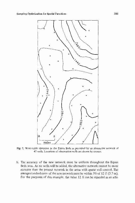
Fig. 7. Water-table elevation in the Equus Beds as perceived by an alternative network of 47 wells. Locations of observation wells are shown by crosses.

b. The accuracy of the new network must be uniform throughout the Equus Beds area. As no wells will be added, the alternative network cannot be more accurate than the present network in the areas with sparse well control. The average standard error of the new network must be within 5% of 12 ft (3.7 m). For the purposes of this example, the value 12 ft can be regarded as an arbi-

386 Olea

4"

4- 4"

4" 4-

4"

4-

+ +

4"4- 4- 4" "P4"

4" 4- + 4-4- 4"

4" 4- 4- 4" 4-4" 4"

41- 4" 4- 4- +

+ *+'+ ( : * f f 4- / g , .v, 4 - 4 " + 4-

4- 4. 4- 4- @ + +

4- 4- + 4- 4 - ' " " " " ~ 4 - 4 - 4- 4" 4" 4.

4- 4 " 4 - 4. + a,l" 4- 4- 4" + 4-

4- 4- + 4- "t-4- 4- 4-

4" , 2 4", 4"4"

4- 4" 4" 4 " + + 4"

4" + 4" 4 - -

4" + 4- 4-

4" 4"

4" 4- 4.

0 5 4"4" + 4"

I J + 4- 4"4" + 4-4"

m i l e s +

4-

+

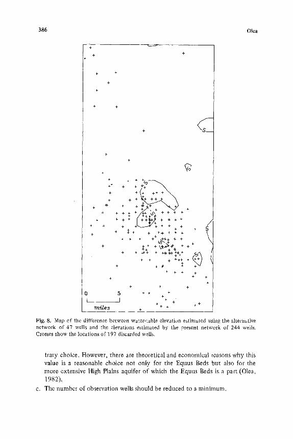
Fig. 8. Map of the difference between water-table elevation estimated using the alternative network of 47 wells and the elevations estimated by the present network of 244 wells. Crosses show the locations of 197 discarded wells.

trary choice. However, there are theoretical and economical reasons why this value is a reasonable choice not only for the Equus Beds but also for the more extensive High Plains aquifer of which the Equus Beds is a part (Olea, 1982).

c. The number of observation wells should be reduced to a minimum.


d. The area estimated by the alternative network should be at least 99% of the area estimated using the present network.

From Table 1, and provided the spatial function is isotropic, the absolute best arrangement of samples is a regular hexagonal pattern. However, the random location o f the existing observation wells precludes a hexagonal pattern or any of the other regular patterns. The next most effective arrangement is a stratified hexagonal pattern. Because it is partly irregular, it has the flexibility required to maximize the use of existing wells.

The alternative network should be designed to have an average standard error somewhat smaller than 12 ft (3.7 m) in most areas to compensate for higher than average standard errors in the areas near the boundaries of the aquifer where no wells exist. The Appendix contains the details of a design with a 10% penalty on the 12 ft (3.7 m) average standard error.

The final sampling design requires the random selection of an observation well from inside each of the 16-square-mile hexagons that cover the Equus Beds area in a regular pattern. Notice that prior structural analysis of the elevation of the water table in the map area was required, but no actual sampling or universal kriging calculations were necessary to design the improved sampling scheme.

Design Verification

Figure 7 shows the sampling design for the alternative network for the Equus Beds. The new network has only 47 observation wells and represents an 81% reduction from the original number of wells. Although the reduction in number of wells is substantial, a comparison of the isolines on maps in Figs. 4

Fig. 9. Relative frequency of the differences between water-table elevations estimated using the alternative network of 47 wells and elevations estimated by the present network of 244 wells. The mean is zero and the standard deviation is 2.6 ft.

40

30

25

20

15

5

I ¸ ~ ....... I.. -]0 -5 0 5 ]0 Difference Between Maps, Ft

388 Olea

and 7 shows that the amount of information lost is minimal, as corresponding isolines are almost identical. The similarity between the maps is emphasized by Fig. 8 which shows that the differences do not exceed 10 ft (3 m) and by Fig. 9 which shows that 95% of the values in the two contour map grids differ by less than 5 ft (1.5 m).

The average standard error increased to 0nly 11.74 ft (3.5 m) in the alternative network, which is within 2.2% of the specified error level of 12 ft (3.7 m).

y.+

x,_

t

Fig. 10. Standard error of the water-table elevation in the Equus Beds as perceived by an alternative network of 47 wells. Locations of observation wells are shown by crosses.


25

Fig. 11. Relative frequency of the standard error of the water-table elevation in the Equus Beds as perceived by the alternative network of 47 wells. The mean is 11.74 ft and the standard deviation is 3.85 ft.

L .

g_ g- C

g

g~

20

15

10

5

/ 0 C

0 lO 20 30 Standard Error, Ft

The improvement in sampling homogenei ty is indicated by the more uniform pat tern o f isolines in Fig. 10 and by the unimodal distribution of the standard error shown in Fig. 11. Note on Fig. 10 that 68.7% of the values are within the interval between 5 ft (1.5 m) and 15 ft (4.5 m). In addit ion there is a 35% reduction in the error variance from 22.8 ft 2 (1.51 m 2) to 14.8 ft 2 (2.11 m2). Table 10 summarizes the characteristics of the present and alternative networks.

RECOMMENDATIONS

Ideally, a sampling pattern should be planned before any measurements are taken, in order to insure that the most efficient design is selected. The absolutely best discontinuous sampling pattern for an isotropic spatial function is a regular hexagonal pattern. If all other factors are held constant, a regular hexagonal pattern possesses the minimum average standard error, the lowest maximum stan-

Table 10. Comparison Between the Present and Alternative Networks

Present Alternative Change

Hexagonal Pattern Random stratified

Number of wells 244 47 -80.7% Average standard error (ft) 9.98 11.74 17.6% Standard error variance (ft 2) 22.8 14.8 -34.9% Nodes estimated 819 823 0.05%

390 Olea

dard error, the maximum screen effect, and requires the minimum number of nearest neighbors to assure a stable solution to the universal kriging system of equations.

Practical considerations may force the use of a regular square pattern, which in certain aspects is marginally inferior to the regular hexagonal pattern, but may be easier to implement. A regular hexagonal pattern will outperform a regular square pattern by 1% in average standard error, and by 3% in maximum standard error. However, a square pattern requires three times more nearest neighbors to reach the point of no additional return in maximum standard error.

Regular sampling should be favored whenever possible and should be a prime objective in the design of new sampling systems. A random pattern, for instance, requires 4.5 times more sampling elements than a regular hexagonal pattern to achieve the same maximum standard error over the sampling domain. The additional data requirements for clustered patterns may be one order of magnitude larger.

CONCLUSIONS

The average and the maximum values of standard error provided by universal kriging can be used as indices of sampling efficiency. These indices depend on unmanageable factors, including the drift and the semivariance of residuals, which are inherent in the spatial variable. The indices also depend upon three factors under control of the experimenter. These are the number of nearest neighbors used in the estimation procedure, the spatial pattern of the sample points, and the density of the points across the mapped area.

The indices decrease slowly and monotonically by increasing the density of sample elements. If other factors remain unchanged, the sample patterns ranked by decreasing level of efficiency are:

1. Regular

2. Stratified

3. Random

4. Clustered

Selection of the best combination of the manageable factors is an operations research problem, which can be solved through a simple systematic procedure. In a practical test, the procedure successfully corrected a case of over- sampling and uneven density of control points.

Determination of the most appropriate levels of sampling efficiency is a decision that should be external to the statistics of sampling. The index level must be selected according to the economics of data gathering, the further uses of the collected information, and the amount of uncertainty that is acceptable in the study.


APPENDIX: SAMPLING DESIGN EXAMPLE

Problem: Find the best sampling procedure for the Equus Beds aquifer which will produce estimates of the water-table elevation having an average standard error of 10.8 ft (3.3 m). The solution must be restricted to a subset of the existing observation wells. Border effects will be ignored.

Solution using Algorithm 1 :

1. From the structural analysis of water-table elevations (Olea, 1982, Appen- dix A), the relevant parameters are: a. co = 60 ft2/mile (3,5 m2/km). b. The drift model is a first-degree polynomial within a neighborhood of

28 miles (45 km).

2. From the statement of the problem, the sampling efficiency index is the average standard error.

3. From the statement of the problem, regular patterns are not feasible. From Table 1, the class of irregular patterns with lowest average standard error are stratified patterns. A hexagonal stratified pattern is preferable over a square stratified pattern because it has a lower maximum standard error. The value I(1, 1) is 0.69 ft (0.21 m).

4. From the statement of the problem, I(co, p) is equal to 10.8 ft (3.3 m).

5. From eq. 1 and the steps above

p = 602(0.69/10.8) 4

= 0.06 points per square mile (0.023 points/km a)

6. The number of points inside a circle with a diameter of 28 miles (45 km), at a density of 0.06 point per square mile (0.023 point/km=), is

N = (zrd2/4) p

= (3.14159 X 282 X 0.06)/4

= 36 points

7. From Table 3, the minimum number of nearest neighbors required to solve the universal kriging system of equations is 3, which is an order of magnitude smaller than the number of points that can be contained inside the neighborhood for which structural analysis models are valid.

8. From Table 2, the point of no return is 6.

9. Since the 36 points that can be placed inside the structural analysis neighborhood is a larger number than the point of no return, 6 nearest neighbors should be used in the solution of the universal kriging system of equations.

Hence, the best irregular sampling pattern for the water-table elevation in the Equus Beds aquifer is a hexagonal stratified pattern. A density of 0.06 points

392 Olea

per square mile (0.023 points /kin 2) assures an average standard error o f 10.8 ft

(3.3 m). The number o f sample elements to be used in the universal kriging sys-

tem of equat ions should be 6.

REFERENCES

Albert, C. D. and Stramel, G. J., 1966, Fluvial sediments in the Little Arkansas River Basin, Kansas: U.S. Geological Survey Water-Supply Paper 1798-B, 30 p.

Alldredge, J. R. and Alldredge, N. G., 1978, Geostatistics: A bibliography: Internal. Stat. Rev., v. 46, p. 77-88.

Clark, P. J. and Evans, R. C., 1954, Distance to nearest neighbors as a measure of spatial relationships in populations: Ecology, v. 35, no. 4, p. 445-453.

James, G. and James, R. C., 1976, Mathematics Dictionary: Van Nostrand Reinhold Com- pany, New York, 509 p.

Journel, A. G. and Huijbregts, C. J., 1978, Mining Geostatistics: Academic Press, London, 600 p.

Matheron, G., 1965, Les variables r6gionalise6s et leur estimation: Masson et Cie, Editeurs, Paris, 305 p.

Matheron, G., 1971, The theory of regionalized variables and its applications: Les Cahiers du Centre de Morphologie Math6matique de Fontainebleau, Fascicule 5, Edit6 par l'Ecole National Sup6rieure des Mines de Paris, 211 p.

Olea, R. A., 1975, Optimum mapping techniques using regionalized variable theory: Karts. Geol. Surv. Series on Spatial Analysis No. 2, University of Kansas, Lawrence, Kansas, 137 p.

Olea, R. A., 1982, Optimization of the High Plains aquifer observation network, Kansas: Kans. Geol. Surv. Ground Water Series No. 7, University of Kansas, Lawrence, Kansas, 73p.

Olea, R. A., (in preparation), Systematic sampling of spatial functions: Kans. Geol. Surv., Series on Spatial Analysis No. 7, University of Kansas, Lawrence, Kansas.

Petri, L. R., Lane, C. W., and Furness, L. W., 1964, Water resources of the Wichita area, Kansas: U.S. Geological Survey Water-Supply Paper 1499-I, 69 p.

Ripley, B. D., 1981, Spatial Statistics: John Wiley & Sons, New York, 252 p. Stramel, G. J., 1956, Progress report on the ground-water hydrology of the Equus Beds

area, Kansas: Kans. Geol. Surv. Bull. 119, Pt. 1, 59 p. Stramel, G. J., 1967, Progress report on the ground-water hydrology of the Equus Beds

area, Kansas: Kans. Geol. Surv. Bull. 187, Pt. 2, 27 p. Williams, C. C. and Lohman, S. W., 1949, Geology and ground-water resources of part of

south-central Kansas: Kans. Geol. Surv. Bull. 79,455 p. Williams, W. H., 1978, A Sampler on Sampling: John Wiley & Sons, New York, 254 p.

Documents

Sampling design optimization for spatial functions of observation...Mathematical Geology, Vol. 16, No. 4, 1984 Sampling Design Optimization for Spatial Functions Ricardo A. Oiea 2