Routing Optimization for Delay Tolerant Networks in

Faculdade de Engenharia da Universidade do Porto

Routing Optimization for Delay

Tolerant Networks in Intelligent

Environments

Constantino Antunes

Tese submetida no ambito do

Mestrado Integrado em Engenharia Electrotecnica e de Computadores

Major de Telecomunicacoes

Orientador: Ricardo Morla

Junho de 2008

-2

c© Constantino Antunes, 2008

i

ii

Resumo

Este trabalho apresenta um estudo sobre routing DTN e possıveis optimizacoes. Saopropostas e testadas tres melhorias ao protocolo PROPHET, mostrando aumentos deentrega de mensagens em torno de 1% e reducao de gasto de recursos em cerca de 1%. Etambem proposto um protocolo hıbrido que mostrou ser capaz de entregar uma quantidadede mensagens acima de 99% do valor maximo possıvel para a rede, ao mesmo tempo queusa apenas mais 0.3% e 0.2% de buffer e largura de banda por mensagem entregue do queo protocolo PROPHET.

iii

iv

Abstract

This work presents a study on DTN routing and possible optimizations. Three improve-ments for the PROPHET protocol are proposed and tested, showing message deliveryincrease around 1% and resource saving around 1%. A hybrid protocol is evaluated andobservations show its capability of delivering an amount of messages above 99% of themaximum delivery possible for the network while exhibiting buffer occupancy and band-width usage cost only 0.3% and 0.2% above that of PROPHET, which is a referenceregarding these two metrics. These results were obtained from data collected in real usagesituations by third-party projects.

v

vi

Acknowledgements

I would like to thank my supervisor, Ricardo Morla, for his countless advices and for hiscontributions for this work. I would also like to thank Nathan Eagle for providing theReality Mining Database.

vii

viii

Contents

1 Introduction 11.1 Context . . . . . . . . . . . . . . . . . . . . . . . . . . . . . . . . . . . . . . 11.2 Goals . . . . . . . . . . . . . . . . . . . . . . . . . . . . . . . . . . . . . . . 21.3 Structure . . . . . . . . . . . . . . . . . . . . . . . . . . . . . . . . . . . . . 2

2 Related Work 52.1 DTN protocols . . . . . . . . . . . . . . . . . . . . . . . . . . . . . . . . . . 52.2 DTN Applications . . . . . . . . . . . . . . . . . . . . . . . . . . . . . . . . 132.3 User’s Context . . . . . . . . . . . . . . . . . . . . . . . . . . . . . . . . . . 142.4 Other related work . . . . . . . . . . . . . . . . . . . . . . . . . . . . . . . . 17

3 Methodology 213.1 Simulator . . . . . . . . . . . . . . . . . . . . . . . . . . . . . . . . . . . . . 21

3.1.1 Addresses . . . . . . . . . . . . . . . . . . . . . . . . . . . . . . . . . 223.1.2 Links and Connections . . . . . . . . . . . . . . . . . . . . . . . . . . 233.1.3 Messages . . . . . . . . . . . . . . . . . . . . . . . . . . . . . . . . . 23

3.2 Traffic models . . . . . . . . . . . . . . . . . . . . . . . . . . . . . . . . . . . 233.3 Networks . . . . . . . . . . . . . . . . . . . . . . . . . . . . . . . . . . . . . 23

3.3.1 UMass . . . . . . . . . . . . . . . . . . . . . . . . . . . . . . . . . . . 243.3.2 Reality Mining . . . . . . . . . . . . . . . . . . . . . . . . . . . . . . 24

3.4 Evaluation metrics . . . . . . . . . . . . . . . . . . . . . . . . . . . . . . . . 243.4.1 Arrivals . . . . . . . . . . . . . . . . . . . . . . . . . . . . . . . . . . 253.4.2 Buffer . . . . . . . . . . . . . . . . . . . . . . . . . . . . . . . . . . . 253.4.3 Xmit . . . . . . . . . . . . . . . . . . . . . . . . . . . . . . . . . . . . 253.4.4 Cost . . . . . . . . . . . . . . . . . . . . . . . . . . . . . . . . . . . . 253.4.5 Metrics discussion . . . . . . . . . . . . . . . . . . . . . . . . . . . . 27

3.5 Simulations . . . . . . . . . . . . . . . . . . . . . . . . . . . . . . . . . . . . 283.6 Work Organization . . . . . . . . . . . . . . . . . . . . . . . . . . . . . . . . 28

4 Comparison Protocols 314.1 Epidemic . . . . . . . . . . . . . . . . . . . . . . . . . . . . . . . . . . . . . 31

4.1.1 Results . . . . . . . . . . . . . . . . . . . . . . . . . . . . . . . . . . 324.1.2 Discussion . . . . . . . . . . . . . . . . . . . . . . . . . . . . . . . . . 33

4.2 DTLSR . . . . . . . . . . . . . . . . . . . . . . . . . . . . . . . . . . . . . . 344.2.1 Results . . . . . . . . . . . . . . . . . . . . . . . . . . . . . . . . . . 344.2.2 Discussion . . . . . . . . . . . . . . . . . . . . . . . . . . . . . . . . . 35

4.3 PROPHET . . . . . . . . . . . . . . . . . . . . . . . . . . . . . . . . . . . . 354.3.1 Results . . . . . . . . . . . . . . . . . . . . . . . . . . . . . . . . . . 36

ix

x CONTENTS

4.3.2 Discussion . . . . . . . . . . . . . . . . . . . . . . . . . . . . . . . . . 374.4 Comparison — UMass . . . . . . . . . . . . . . . . . . . . . . . . . . . . . . 374.5 Reality Mining Results . . . . . . . . . . . . . . . . . . . . . . . . . . . . . . 41

4.5.1 Epidemic Results . . . . . . . . . . . . . . . . . . . . . . . . . . . . . 414.5.2 PROPHET Results . . . . . . . . . . . . . . . . . . . . . . . . . . . . 42

4.6 Comparison — Reality Mining . . . . . . . . . . . . . . . . . . . . . . . . . 43

5 Changes to PROPHET 455.1 EQ-GRTR . . . . . . . . . . . . . . . . . . . . . . . . . . . . . . . . . . . . . 45


5.2 Fast Start . . . . . . . . . . . . . . . . . . . . . . . . . . . . . . . . . . . . . 475.2.1 Results . . . . . . . . . . . . . . . . . . . . . . . . . . . . . . . . . . 475.2.2 Discussion . . . . . . . . . . . . . . . . . . . . . . . . . . . . . . . . . 48

5.3 Estimated Delivery Confirmation (EDC) . . . . . . . . . . . . . . . . . . . . 495.3.1 Results . . . . . . . . . . . . . . . . . . . . . . . . . . . . . . . . . . 505.3.2 Discussion . . . . . . . . . . . . . . . . . . . . . . . . . . . . . . . . . 51

5.4 Conclusions . . . . . . . . . . . . . . . . . . . . . . . . . . . . . . . . . . . . 51

6 Hybrid Protocol 536.1 Decision limit . . . . . . . . . . . . . . . . . . . . . . . . . . . . . . . . . . . 54

6.1.1 Results . . . . . . . . . . . . . . . . . . . . . . . . . . . . . . . . . . 546.1.2 Discussion . . . . . . . . . . . . . . . . . . . . . . . . . . . . . . . . . 576.1.3 Limit decision . . . . . . . . . . . . . . . . . . . . . . . . . . . . . . . 58

6.2 Behaviour analysis . . . . . . . . . . . . . . . . . . . . . . . . . . . . . . . . 606.3 Validation . . . . . . . . . . . . . . . . . . . . . . . . . . . . . . . . . . . . . 61


6.4 Conclusions . . . . . . . . . . . . . . . . . . . . . . . . . . . . . . . . . . . . 63

7 Conclusion 657.1 Methodology Evaluation . . . . . . . . . . . . . . . . . . . . . . . . . . . . . 657.2 Contribution Evaluation . . . . . . . . . . . . . . . . . . . . . . . . . . . . . 66

7.2.1 Metrics . . . . . . . . . . . . . . . . . . . . . . . . . . . . . . . . . . 667.2.2 PROPHET changes . . . . . . . . . . . . . . . . . . . . . . . . . . . 667.2.3 Hybrid Protocol . . . . . . . . . . . . . . . . . . . . . . . . . . . . . 67

7.3 Future Work . . . . . . . . . . . . . . . . . . . . . . . . . . . . . . . . . . . 67

References 71

List of Figures

2.1 Number messages and delivery delay results from [2] . . . . . . . . . . . . . 72.2 Queuing time results from [3] . . . . . . . . . . . . . . . . . . . . . . . . . . 82.3 Messages results from [4] . . . . . . . . . . . . . . . . . . . . . . . . . . . . 92.4 Delivery delay results from [4] . . . . . . . . . . . . . . . . . . . . . . . . . 102.5 Message delivery delay results from [9] . . . . . . . . . . . . . . . . . . . . . 122.6 Message delivery delay results from [10] . . . . . . . . . . . . . . . . . . . . 122.7 Pairs encounter results from [19] . . . . . . . . . . . . . . . . . . . . . . . . 142.8 Pairs encounters per hour from [19] . . . . . . . . . . . . . . . . . . . . . . 152.9 Average pairs encounters per day from [19] . . . . . . . . . . . . . . . . . . 152.10 Real and synthetic trace from [19] . . . . . . . . . . . . . . . . . . . . . . . 162.11 Protocol results from [19] . . . . . . . . . . . . . . . . . . . . . . . . . . . . 172.12 Throughput in function of bundle size from [24] . . . . . . . . . . . . . . . 18

3.1 DTN2 classes . . . . . . . . . . . . . . . . . . . . . . . . . . . . . . . . . . . 22

4.1 Epidemic vs Flood, day 1 of UMass network . . . . . . . . . . . . . . . . . . 324.2 Epidemic, Umass network . . . . . . . . . . . . . . . . . . . . . . . . . . . . 334.3 Epidemic, Umass network . . . . . . . . . . . . . . . . . . . . . . . . . . . . 334.4 DTLSR, UMass network . . . . . . . . . . . . . . . . . . . . . . . . . . . . . 344.5 DTLSR, UMass network . . . . . . . . . . . . . . . . . . . . . . . . . . . . . 354.6 PROPHET, UMass network . . . . . . . . . . . . . . . . . . . . . . . . . . . 364.7 PROPHET, UMass network . . . . . . . . . . . . . . . . . . . . . . . . . . . 374.8 Comparison, day 1 of UMass network . . . . . . . . . . . . . . . . . . . . . 384.9 Comparison, day 2 of UMass network . . . . . . . . . . . . . . . . . . . . . 384.10 Comparison, day 3 of UMass network . . . . . . . . . . . . . . . . . . . . . 384.11 Comparison, day 1 of UMass network: costs . . . . . . . . . . . . . . . . . . 394.12 Comparison, day 2 of UMass network: costs . . . . . . . . . . . . . . . . . . 394.13 Comparison, day 3 of UMass network: costs . . . . . . . . . . . . . . . . . . 404.14 Comparison, UMass network: DTLSR’s costs relative to Epidemic . . . . . 404.15 Comparison, UMass network: PROPHET’s costs relative to Epidemic . . . 404.16 Epidemic, Reality Mining network . . . . . . . . . . . . . . . . . . . . . . . 414.17 Epidemic, Reality Mining network . . . . . . . . . . . . . . . . . . . . . . . 414.18 PROPHET, Reality Mining network . . . . . . . . . . . . . . . . . . . . . . 424.19 PROPHET, Reality Mining network . . . . . . . . . . . . . . . . . . . . . . 424.20 Comparison, PROPHET relative to Epidemic . . . . . . . . . . . . . . . . . 42

5.1 EQ-GRTR, UMass results . . . . . . . . . . . . . . . . . . . . . . . . . . . . 465.2 EQ-GRTR, Reality Mining results . . . . . . . . . . . . . . . . . . . . . . . 465.3 Fast Start, UMass results . . . . . . . . . . . . . . . . . . . . . . . . . . . . 48

xi

xii LIST OF FIGURES

5.4 Fast Start, Reality Mining results . . . . . . . . . . . . . . . . . . . . . . . . 485.5 EDC, UMass results . . . . . . . . . . . . . . . . . . . . . . . . . . . . . . . 505.6 EDC, Reality Mining results . . . . . . . . . . . . . . . . . . . . . . . . . . . 50

6.1 Hybrid Router . . . . . . . . . . . . . . . . . . . . . . . . . . . . . . . . . . 546.2 Hybrid Router, UMass arrivals . . . . . . . . . . . . . . . . . . . . . . . . . 556.3 Hybrid Router, UMass buffer cost . . . . . . . . . . . . . . . . . . . . . . . 556.4 Hybrid Router, UMass xmit cost . . . . . . . . . . . . . . . . . . . . . . . . 566.5 Hybrid Router, Reality Mining arrivals . . . . . . . . . . . . . . . . . . . . . 566.6 Hybrid Router, Reality Mining buffer cost . . . . . . . . . . . . . . . . . . . 566.7 Hybrid Router, Reality Mining xmit cost . . . . . . . . . . . . . . . . . . . 576.8 Hybrid Router, small limits tests . . . . . . . . . . . . . . . . . . . . . . . . 586.9 Hybrid Protocol, ε = 0.5 . . . . . . . . . . . . . . . . . . . . . . . . . . . . . 596.10 Hybrid Protocol, ε = 0.5 . . . . . . . . . . . . . . . . . . . . . . . . . . . . . 596.11 Hybrid Protocol, ε = 0.5 . . . . . . . . . . . . . . . . . . . . . . . . . . . . . 596.12 Reality Mining, week days and arrivals . . . . . . . . . . . . . . . . . . . . . 606.13 Reality Mining, pairs . . . . . . . . . . . . . . . . . . . . . . . . . . . . . . . 616.14 Hybrid validation, arrivals . . . . . . . . . . . . . . . . . . . . . . . . . . . . 626.15 Hybrid validation, buffer-cost . . . . . . . . . . . . . . . . . . . . . . . . . . 626.16 Hybrid validation, xmit-cost . . . . . . . . . . . . . . . . . . . . . . . . . . . 62

List of Tables

3.1 Umass network contacts and nodes . . . . . . . . . . . . . . . . . . . . . . . 243.2 Reality Mining network months . . . . . . . . . . . . . . . . . . . . . . . . . 253.3 Reality Mining network contacts and nodes . . . . . . . . . . . . . . . . . . 263.4 Cost and its relation with arrivals . . . . . . . . . . . . . . . . . . . . . . . . 263.5 Cost and its relation with arrivals, simplified table . . . . . . . . . . . . . . 273.6 Umass network contacts and nodes, between 6 and 12 am . . . . . . . . . . 283.7 Reality Mining network contacts and nodes, between 6 and 12 am . . . . . 28

5.1 EQ-GRTR’s GRTR ratio . . . . . . . . . . . . . . . . . . . . . . . . . . . . 475.2 Fast Start’s PROPHET ratio . . . . . . . . . . . . . . . . . . . . . . . . . . 495.3 EDC’s PROPHET ratio . . . . . . . . . . . . . . . . . . . . . . . . . . . . . 51

6.1 Reality Mining network week days, contacts and nodes . . . . . . . . . . . . 586.2 Hybrid protocol, Epidemic’s ratio averages . . . . . . . . . . . . . . . . . . . 606.3 Reality Mining pairs, average and deviation . . . . . . . . . . . . . . . . . . 616.4 Validation, average and deviation . . . . . . . . . . . . . . . . . . . . . . . . 626.5 Validation, Protocols Comparison . . . . . . . . . . . . . . . . . . . . . . . . 636.6 Validation, Epidemic’s ratio averages . . . . . . . . . . . . . . . . . . . . . . 63

xiii

xiv LIST OF TABLES

Chapter 1

Introduction

1.1 Context

Computational devices share data through wired or wireless links. Whenever a devicetries to send data, it uses that link to determine if the destination is reachable. If it is not,the communication fails. Traditional network protocols do not solve this problem. Forexample, ad-hoc protocols are useful in mobility scenarios but do not work when networknodes disappear and partition the network. This happens because these protocols aredesigned with the assumption of permanent links and are useless to communicate in anenvironment where data is lost because connections are intermittent.

Being carried by people, personal wireless devices will see their location change withtime, possibly moving out of range of any access point. Ideally, one would want to providenetwork connectivity without restricting users mobility. The obvious solution would be toplace enough access points to cover the desired area, guaranteeing that there would alwaysbe a network connection. However, the area may be too large or not easily accessible, bywhich deploying the necessary access points would not make economic sense.

An approach to provide network connectivity in such partitioned networks is for thedevice which is sending the data to store that data until an available link is found. Thenode which receives the data should be able to wait for another connection to pass it on.This kind of network is called a Delay Tolerant Network (DTN), a kind of network thatconnects devices that have the ability to store information and forward it when a receiveris found. This way, even when no access point is reachable and there is not permanentlinks, communication is still possible.

Besides the simple description of a DTN, routing on it is very difficult. Consider anarea of arbitrary size with people moving inside it. Each person carries a device capableof communicating with other devices. Consider also that each device has no knowledge

1

2 Introduction

of its movements nor other devices movements. On this scenario, routing a message fromone device A to a device B means that A may choose to wait for a connection with B orsend the message to other devices, hoping that they will deliver it to B. The second optionseems to offer greater probability of message delivery. But, to which devices should themessage be sent? Should it be sent to all devices met or a limited number? Should it becopied or not?

1.2 Goals

Any successful communication network has to be able to deliver data with low error ratewhich is essential for the messages to reach their destination and do that with its infor-mation untouched. The data should also be delivered as fast as possible and any requiredrouting data should be kept in minimum quantities so the transmission medium is opti-mized for message delivery.

This work’s objectives were to study approaches on DTN routing, improve them andbuild a protocol that combines the better protocols studied. These objectives were ac-complished having in mind the requirements for general communication network applyingthem on the DTN context:

1. Maximize arrivals — this requirement is equivalent to the referred low error ratenecessary for any network;

2. Minimize buffer occupancy — since a DTN node saves messages for future de-livery, the space for message storage is essential and should be saved;

3. Minimize transmissions — the transmission medium should be saved so messagesare transmitted as fast as possible between nodes.

It is also important to minimize the delivery delay, but that is more dependent on thenetwork and frequency of node contacts itself than the routing protocol.

1.3 Structure

Approaches to answer the questions in section 1.1 were proposed on previous work andare presented in the next chapter. The related work provided information on successfulrouting protocols and the data used for realistic simulation. The details on the decisionsdone for tests and evaluation are presented in chapter 3.

Before optimize or create new protocols, a chosen number of them were tested (chap-ter 4). These tests allowed validation of implemented protocols and the simulator itself.After choosing and testing protocols, optimization approaches were experimented and the

1.3 Structure 3

results are presented in chapter 5. The combination of two protocols resulted into a newprotocol (described and validated in chapter 6) which exhibits the best features of bothbase protocols.

4 Introduction

Chapter 2

Related Work

Related work on this subject is rich, many articles may be found at the Delay TolerantResearch Group (DTNRG) web site [1]. This chapter is divided into four sections. Thefirst presents related work on diverse routing protocols. The second refers some applica-tions of DTN. Section 3 presents related work on user context and section 4 presents otherpapers that, while not directly related to this work, provide different views about DTNsthat might be considered.

2.1 DTN protocols

A study about a scenario where nodes are free to move and do not have information abouttheir neighbours is done in [2]. This work is about a successful albeit simple protocolcalled Epidemic Protocol. It consists of spreading the data like a disease for all nodes ora maximum number of nodes. Two assumptions are made in [2]:

1. Nodes are blind — meaning they do not have any external information about othernodes;

2. Nodes are independent — which means that nodes movement do not depend of othernode’s movement. Other works to be presented in this section observe that this isnot a real situation but it was useful in the context of [2].

A metric called willingness was associated to each node. This metric reflects thewillingness of a node to participate in messages forwarding. Four schemes for messagespreading control were introduced as well:

1. Basic Probabilistic (BP) — uses of an uniform probabilistic function to determinethe willingness of a node;

2. Time to Live (TTL) — the maximum number of hops for each message, when TTLreaches zero the message is discarded;

5

6 Related Work

3. Kill Time — after this time the message is discarded;

4. Passive Cure — when the destination receives a message, sends an ACK which iscopied to each node trying to send the already received message.

The evaluation metrics included the number of messages sent by each node and themessage delivery delay. As can be seen in figure 2.1, BP generates the largest number ofmessages in the system. Other schemes added to BP allow less volume of messages, thebetter being BP + TTL + Passive Cure. It would be interesting to evaluate other schemeswithout BP.

Other approach to the same problem of creating message delivery confirmation ispresented in [3]. This is done with four testing schemes:

1. Hop by Hop — each node sends an ACK to the node from which it received the mes-sage. This does not provide end to end reliability and was only used for comparisonpurposes;

2. Active Receipt — generates an ACK which behaves like any other message, beingsprayed to all nodes;

3. Passive Receipt — generates an ACK sent only when a node tries to forward amessage already delivered;

4. Network-Bridged Receipt — generates an ACK sent by cellular network. This re-quires all nodes to have a cellular network interface.

Simulation results are displayed in figure 2.2. The best scheme offering end-to-endreliability was Network-Bridged and the best scheme not requiring an external networkwas Active Receipt, considering the average queuing time as evaluation metric.

Despite the simplicity of the Epidemic Protocol, it uses excessive bandwidth. Thisproblem is analysed in [4] which proposed a new protocol called PROPHET that does notrequire copying all messages to all nodes and can offer a similar performance to that of theEpidemic Protocol. This is a probabilistic type of routing, a way for the nodes to decideto which nodes they will forward messages based in the probability of successful messagedelivery. The routing metric, called predictability , was calculated on the history of nodesencounters and associated to each node and each destination. An ageing constant correctspredictability’s value when nodes do not meet before a certain amount of time, and atransitivity effect which affects a node’s predictability with other nodes predictabilities.The example given in [4] is: if a network node A meets a node B frequently and Bmeets node C frequently, then A has a high predictability when delivering messages to Ceven if A has a low probability of seeing C. The simulation introduced a scenario calledCommunitary Model in which network nodes movements are based in people’s movements.

2.1 DTN protocols 7

Figure 2.1: Number messages and delivery delay results from [2]

8 Related Work

Figure 2.2: Queuing time results from [3]

In this model, each node has a place which it visits frequently and all nodes have a commonGathering Place where they all meet. This tries to simulate movements similar to peopletravelling from home to work. The PROPHET protocol was simulated in the referredscenario and in a completely random scenario. The Epidemic protocol was simulated too,for comparison purposes. The evaluated metrics were the number of forwarded messages(figure 2.3) and delay (figure 2.4) against the queue size. PROPHET shows better resultsin the communitary model and equivalent results in the random model.

Another approach to random mobility protocols called MoVe is analysed in [5] andcompared against two simple protocols:

1. Broadcast — similar to Epidemic.

2. NoTalk — the carrier is only allowed to forward the message to the ultimate desti-nation.

The MoVe protocol is a geographical form of routing that uses node position and velocityto forward messages to other nodes moving into the message’s destination position. Thisprotocol suffers from the lack of knowledge about the future movements of nodes and thelack of knowledge about the position of the message destination, when starting a commu-nication. Results show performance between the other two protocols.

An integration of DTN with AODV is presented in [6]. The strategy is to use AODV,which is an ad-hoc distance vector protocol, to find routes. With this scheme, nodes useend-to-end connection when the found route allows that. The same mechanism used tofind AODV routes also deliver information about DTN reachability. This means that evenwhen no end-to-end route is found, it is possible for a node to reach a destination through

2.1 DTN protocols 9

Figure 2.3: Messages results from [4]

10 Related Work

Figure 2.4: Delivery delay results from [4]

2.1 DTN protocols 11

DTN routing. This network may be viewed as an ad-hoc network composed by a cloudof network nodes. When a node needs to send a message to other node that is not in thecloud it uses DTN routing. Simulations of this system included a scenario having networknodes with random movement without stops and speeds up to 20m/s. Results showedthat AODV links using TCP dominated.

A probabilistic solution based in Kalman filters for network nodes encounter predictionis presented in [7]. The advantage of this prediction technique is that it does not requirefull knowledge of nodes encounters history to predict the next encounter. Instead, it uses aKalman filter which is a filter from control theory that uses a system input to estimate theexpected output value for that system. Then, the system’s real output is used to correctthe estimation. This filter uses only the system state to predict its output values and hasgood results even when dealing with unknown system model and non-linear systems [8].The evaluated metrics were queue size, delivery ratio and delay. The results show thatthe proposed protocol (CAR) successfully delivered less messages than Epidemic Protocolbut required less buffer bandwidth and has lower delay associated to message delivery.

[9] presents a protocol for predictable routes. In order to do that, a study on theeffects of additional information over the network performance was done. A way to provideinformation to network nodes, or oracles,was created. The provided information was aboutnodes contacts connections, contacts statistics, queues occupancy and traffic demand.Three types of routing were defined:

1. Zero Knowledge — using no oracles;

2. Partial Knowledge — using one or more oracles except traffic oracle;

3. Full Knowledge — using all oracles.

Since the first two are the more realistic when considering the possibility of implemen-tation, the attention was devoted to them. Some protocols were defined and the resultsshown that the best was EDLQ (Earliest Delivery with Local Queuing) (figure 2.5) whichuses Contacts Oracle to calculate neighbours delay. This protocol also takes into accountthe local queue occupancy and uses a modified Dijkstra algorithm to calculate new pathsevery time a node is met, since optimal routes change with time. Dijkstra’s algorithmis commonly used in link-state protocols to choose between a set of paths the one whichhas minimum cost. Calculations are done with data sent by routers but, in the case of aDTN that data is often out-of-date therefore, the modified version of Dijkstra’s algorithmpresented in [9] may provide benefits to network performance. Also, before the end of thepaper is suggested that the best protocol choice for this scenario should have informationabout the contacts history, which is a challenge in partitioned systems.

12 Related Work

Figure 2.5: Message delivery delay results from [9]

Some link-state protocols are analysed in [10] with the objective of determining whichis the best protocol for a slow, predictable mobility scheme. This was done with theconversion of a standard link-state protocol into a delay tolerant link-state protocol byintroducing longer lifetime Link-State Advertisement (LSA) messages, longer lifetime ofusers messages and best path calculation that includes links which may not be reachable atthe calculation time. The protocol, called DTLSR performed much better than commonlink-state protocol.(figure 2.6)

Figure 2.6: Message delivery delay results from [10]

The details of a predictable mobility scenario simulation are studied in [11]. This workcollected data from 40 buses of DieselNet network that surrounds the UMass AmherstCampus. The results were collected applying Epidemic protocol with active cure for mes-sage spreading control and the metrics presented were the delay, number of copies madeand number of hops each messages done. Models for cyclic movement were created andthe one which shown results closer to the real scenario was the Route-Level model. This

2.2 DTN Applications 13

and other traces may be found in [12] which may be useful to build a network model.This work also shown that it is important to have a detailed model to achieve trustworthyresults.

2.2 DTN Applications

DTN is a kind of network that expects delay in messages delivery. Having that said, itseems clear that it won’t perform very well with streaming communications such as videoconference. This kind of network should have better performance with asynchronousapplications instead of synchronous ones. Related work on this matter presents mostlydistributed file systems for disaster scenarios [13] where redundancy is needed and a flex-ible network that is resistant to partitioning that often occurs in such situations. Theproposed application is a knowledge repository about e.g. medical techniques to use inemergency situations. The results shown that random copies to several network nodes aremore resistant to network partitioning and node loss.

The possibility to use queued messages in DTN routers as cached content for fasteraccess is studied in [14]. This shown that some copies of messages sprayed through thenetwork may also be used as cache and will improve network’s performance. This onlyapplies to answer messages which should have some usable content and it won’t apply toprivate information which should be encrypted.

Tests on the performance of a DTN transporting HTTP was presented in [15]. HTTPwas not modified, which allowed to use common web browsers (Firefox web browser wasused), and web cache proxies with DTN routers. The paper ends with the observationthat the HTTP over DTN system has similar performance of HTTP over TCP when nolatency is present. This is important because it means that a mobile user may choose touse DTN all the time instead of switching to fixed mode of operation. A similar logic isexploited in [16]: the possibility of provide intermittent Internet access in highways. Thediscussion presented the situation of an highway having access points sprayed along it andtravelling cars which would find the access point signal announcing network, connect tothe network and request/download web pages. The main problems are car’s velocity andnetwork hardware range. This limits the amount of time each car have network connectionand consequently the quantity of downloadable information.

[17] presents a system capable of increasing the network performance by introducingawareness of network context. This context awareness refers to the type of informationbeing transferred and network performance. The objective was to build a system capableof adapting itself to the demanded traffic. The system should detect abnormal situations

14 Related Work

degrading network performance such as nodes failures (one example gave in the referredarticle was a meteorite shower). After such situations are detected, the presented systemshould enter an evaluation phase in which it decides either to use other protocol capableof performing better in the new context or abort the transmission.

A DTN security problem is studied in [18]. In this kind of network, because connectiontime and link bandwidth are limited, it may be necessary to use message fragmentation tooptimize link usage. [18] presents some schemes to guarantee that a fragment sent over alink is not a waste of bandwidth. However, this requires further work. In our work we willconsider that fragmentation won’t occur and will assume that the DTN will be deployedin a secure environment.

2.3 User’s Context

As already noticed in previous works, network nodes do not move randomly. The realsituation is that each is owned by a person having a home, work and friends. People havetheir own routines, for example they have a week-day routine of going to work but atnight it is common for everyone to go home. It is reasonable to think that at weekendsthe behaviour changes. This situation is exploited in [19] which uses data from [20] todetermine patterns in peoples behaviour and separate the studied environment into twoclasses — friends and strangers , based in encounter probability (figure 2.7). In this

Figure 2.7: Pairs encounter results from [19]

analysis it was observed that during week days encounters occur more often at afternoonshaving a peak at 16:00 (figure 2.8) while weekends have lower activity (figure 2.9) beingthis greater at late afternoons and evenings.

2.3 User’s Context 15

Figure 2.8: Pairs encounters per hour from [19]

Figure 2.9: Average pairs encounters per day from [19]

16 Related Work

With this and other analyses a simulator was created and validated showing similartrace generation (figure 2.10).

Figure 2.10: Real and synthetic trace from [19]

This simulator was used with four DTN protocols:

1. Direct contact — only forward to the final destination;

2. Forward to 1 person — the message is allowed to be forward only once;

3. Forward to 2 persons — the same as the previous but two forwards are allowed;

4. Forward to all — this scheme forward messages to all friends.

Epidemic protocol was also implemented for comparison purposes. Results show thatin the presence of social information all routing protocols perform much better having”forward to all” the lowest delay, being only surpassed by Epidemic Protocol (figure 2.11).

Other analyses were done in [19] such as use social information to improve firewallsand file-sharing in P2P systems.

Another approach to the problem is absolute positioning of network nodes. This iswhat was tried in [21] where the encountered solution was to learn patterns in paths de-scribed by persons. Network nodes positions were determined assuming that all nodes hada global positioning system (GPS) and creating a simulation software to test the predic-tion technique. The learning techniques were used to build a new protocol (PGR) whichwas tested against other Epidemic-like protocols: Epidemic and three variations of Sprayand Wait. PGR showed good efficiency results, not requiring all nodes to participate inmessages delivery and delivery ratio success close but lower Epidemic’s.

2.4 Other related work 17

Figure 2.11: Protocol results from [19]

2.4 Other related work

A study on the influence of network nodes movements in the network performance is donein [22]. The objective was to study the possibility to use automated nodes that wouldtravel to the place where traffic demand is higher and act as DTN router. The analogyused was taxicabs picking messages as it were passengers.

[23] presents the generic problems associated with Delay-Tolerant Networks. Itemsfrom this work to have in mind are:

1. reliability — this is intended to guarantee that all messages will reach the destination,although it is not always possible to do that being required some form of deliveryconfirmation;

2. delay — this is associated to asynchronous message delivery typical in DTN andshould be minimized;

3. routing — this can be opportunistic, given that it is impossible for a network nodeto always know the optimal route for a message.

The hardware limits imposed by the technology required to create this kind of networkare analysed in [24]. This interesting analysis is directed to the DTN Reference Imple-mentation (DTNRI or DRI) by the IRTF Delay Tolerant Research Group (DTNRG) [1]on low powered devices. It ends with the conclusion that the most restrictive piece ofhardware is the CPU. Also, it was found that bundle (a message or group of messagesto be delivered when two nodes meet) size increases throughput but only until a size of25KB, after that the increase in performance being minimal (figure 2.12).

The paper ends with the following recommendations:

18 Related Work

Figure 2.12: Throughput in function of bundle size from [24]

1. DRI application developers should use the largest possible bundle size when using theDRI in-memory API;

2. The DRI should be restructured to increase parallelism. - use a multi-threaded router;

3. When deploying the DRI, invest more in the CPU than faster storage and increasedmemory.

[25] is a paper about a naming architecture of a DTN. This is an important item, sincewe need to have some way to localize the network nodes. However this is out if the scopeof this work, here we will consider that the naming problem is solved and concentrate inthe routing problem.

The power management of network nodes is studied in [26]. This is closer to the phys-ical level, although, it is still important to understand the communication delay caused bytechnological limits as seen in [24]. The work in [26] explores the idea of using two typesof radio devices: one low powered with high range and high communication error rate forneighbourhood discovery and one with great power consumption with low range but withlow communication error rate. This power management needs more information about thenetwork behaviour so that nodes could use previous knowledge about low network activityto start power-saving modes. This hypothesis is also explored in [26] with the traffic-awarepower management.

The concept of DTN Throwbox is presented in [27] and the problem of energy savingis studied in order to achieve high nodes detection while preserving battery charge. This

2.4 Other related work 19

includes most ideas from the work presented in the last paragraph and is applied to dedi-cated fixed hardware — the DTN Throwboxes — built to act as additional forwarders toimprove network performance.

20 Related Work

Chapter 3

Methodology

In order to optimize routing protocols, it is necessary to study them. For that is requireda simulator, adequate traffic models, networks and evaluation metrics.

On this work was considered that network nodes storage size and connection bandwidthare infinite. These are common simplifications done on previous work. Measures of usedstorage and bandwidth should indicate the hardware required for the DTN to work withthe observed performance.

3.1 Simulator

The simulator used was DTNSim, which is part of the reference implementation DTN2by the DTNRG [1]. The advantages include:

1. It already has protocols implemented;

2. Was built for DTN simulation, unlike other simulators targeted for general networks;

3. Implemented routers may be loaded by the DTN2 daemon to be used on real net-works.

The simulations are defined in .conf files written in TCL scripting language [28]. Acommand ‘sim’ is provided to create nodes and edit simulation options. Each node cre-ated has its own commands to set internal variables and execute other actions. The eventswritten in the .conf file and other events lauched by network nodes go into a stack of eventseach one with a time associated to it. Therefore, the simulator is event-based, having atimer that triggers the event when its time is reached.

The core of DTN2 daemon is the class BundleDaemon, which loads the necessaryclasses for the selected router to work. DTNSim creates a Node object that descends fromthe BundleDaemon. The router object integration within the Node object is similar towhat is done by the BundleDaemon. This way, any router created for DTNSim can be

21

22 Methodology

used on DTN2 daemon. However the opposite is not always true and that is why not allprotocols provided by DTN2 did work with DTNSim.

Figure 3.1 shows classes hierarchy, the ‘my’ namespace was created for new protocolsimplemented during this work.

Figure 3.1: DTN2 classes

DTN2 uses Singleton, a class that can be instantiated only once, as superclass forvarious classes such as BundleDaemon, BundleStore which is used for bundle storage, andRegistrationStore for endpoints registration. Using Singleton objects ensures that criticalresources will not be duplicated but, for simulation, such resources have to be duplicatedwhich raises a problem.

When a new DTN2 daemon is created, a BundleDaemon object is created (amongother objects) which owns a BundleRouter object. When DTNSim runs, several nodesare created and each is a BundleDaemon that behaves like a real DTN2 daemon runningon a separated machine. Because the BundleDaemon class is a Singleton nodes cannotrun in parallel, which prohibits the usage of threads, and each node have to force theirBundleDaemon instance into the BundleDaemon class when its events are to be processed.

3.1.1 Addresses

A DTN node is identified by an ‘eid’ and may have several ‘endpoints’. The eid is anidentifier, similar to the name given to nodes on other types of networks. An eid looks likea web address and starts with the protocol used (dtn), then ‘://’ and after that is placedthe node name. An example of an eid is ‘dtn://alice’.

Other types of networks associate addresses to connections. Endpoints are like thoseaddresses but, since on a DTN connections are intermittent, endpoints are associated tothe data flow. The endpoint address is composed by the eid, followed by ‘/’, followed by theendpoint name. An example of an endpoint address is ‘dtn://alice/work’. If another node‘bob’ tries to send a message to ‘alice’ it must define a source endpoint and a destinationendpoint, for example: from ‘dtn://bob/home’, to ‘dtn://alice/work’.

3.2 Traffic models 23

3.1.2 Links and Connections

DTNSim nodes, like other types of network nodes, are required to have links in orderto establish connections. Each link is associated to a pair of nodes, identified by theireids. Links are created with a command ‘link’ that may also be used to set its availabilityand other parameters. A global command ‘conn’ is provided by the simulator to setconnections between two nodes up and down.

3.1.3 Messages

A network is useless if there is no messages traveling through it. DTNSim provides acommand ‘tragent’ to generate messages and set its size, source, destination and otheroptions. Each generated message had a fixed size of one thousand of bytes (1KB).

3.2 Traffic models

On this work was considered that the simulated DTN will be used for Internet access.Therefore, on the simulation scenarios there are many movable nodes and one fixed accesspoint. A real network may have multiple access points, but the delay to communicatethrough the Internet is much lower than that of a DTN so was considered that all accesspoints behave as a single access point.

The frequency of messages and their size are more difficult to simulate [29]. Becausethe evaluation requires an environment with control over messages, a ‘step’ traffic modelwas used instead a more realistic traffic model.

From systems control theory, an impulse is a burst of energy with infinite amplitudeand zero duration. In practice this means a burst with maximum energy possible and thesmallest duration possible. On a network this means all nodes sending one message at thesame time. Again, from the control theory a step is an array of impulses.

Using the step traffic model means that from time to time all nodes will send a messageto the access point. The network performance to this type of input is the system’s stepresponse. A correct selection of time between each impulse may allow more or less pathexploring, however this was not tested and one impulse by hour was used.

3.3 Networks

This work used real data for network representation on DTNSim. A realistic networkmovement is important because, since we are not restricting buffer size, the protocol isinfluenced by nodes connections not their traffic demand. If each node has infinite buffer,the quantity of messages to deliver is not important. What matters are the paths availableto deliver those messages. If the network node is not realistic those paths may not exist in

24 Methodology

realistic quantities. Also, each society is different which leads to different results on othersets of traces. But the use of a realistic trace of connections should make results muchcloser to what is expected to obtain in reality than artificial networks would have. Twosources of network data were used.

3.3.1 UMass

Several sets of traces of this network are available at [12]. The data used was collectedduring the Spring of 2007 and includes two sets of traces: the one called ‘DieselNet -Spring 2007’ and ‘DieselNet - Access Point Connectivity’. The three days traces of accesspoint connectivity were combined with the Spring 2007 traces and those days (26, 27 and28 of March 2007) were used to create a representation of the UMass network with itsbuses and access points. The text files downloaded from the web site were parsed and thedata was stored into a MySQL database. The total number of contacts is 2.594, table 3.1shows the number of contacts by day and the number of buses on the same day.

Table 3.1: Umass network contacts and nodesDay Contacts Nodes

1 682 252 1.140 293 772 23

3.3.2 Reality Mining

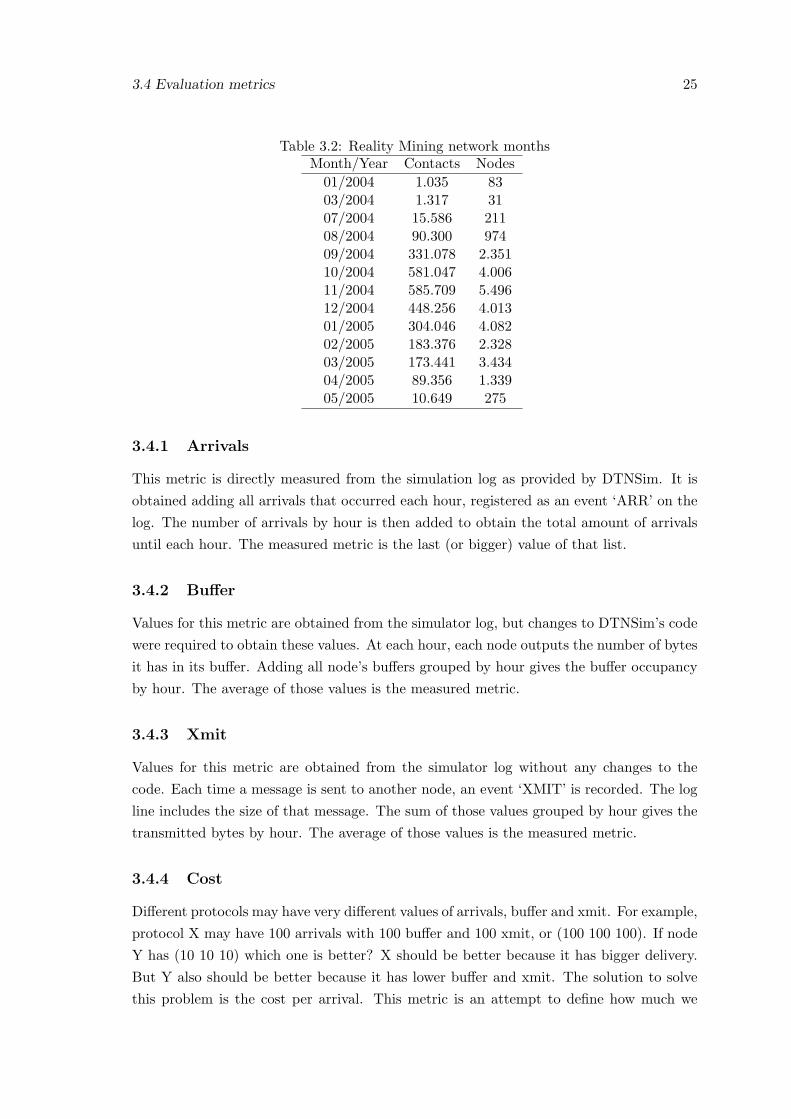
The Reality Mining database, from [20] has a total of 2.815.196 contacts. The contactstable was built with the data of connections between people’s devices, and the data ofconnections between people’s devices with cell towers. Cell towers were used as accesspoints for this network. Table 3.2 shows the number of contacts and nodes for all monthson the database. Table 3.3 shows the contacts and nodes by day for the first ten days ofa randomly selected month (October of 2004).

The selected month was chosen among the months with greater contacts and nodes,months 09/04, 10/04, 11/04, 12/04, 01/05, 02/05 and 03/05. This is necessary for repre-sentation of a network on its activity peak, despite being a disadvantage when we considerthe real simulation time required to simulate such high number of nodes and contacts.

3.4 Evaluation metrics

In order to correctly measure performance, evaluation metrics related to performanceare also required. The metrics measured were the total number of arrivals (Arrivals),the average per hour storage occupancy (Buffer) and the average per hour transmissions(Xmit). Both buffer and xmit metrics are measured in thousands of bytes. Another metricwas calculated from the three metrics referred: cost per arrival.

3.4 Evaluation metrics 25

Table 3.2: Reality Mining network monthsMonth/Year Contacts Nodes

01/2004 1.035 8303/2004 1.317 3107/2004 15.586 21108/2004 90.300 97409/2004 331.078 2.35110/2004 581.047 4.00611/2004 585.709 5.49612/2004 448.256 4.01301/2005 304.046 4.08202/2005 183.376 2.32803/2005 173.441 3.43404/2005 89.356 1.33905/2005 10.649 275

3.4.1 Arrivals

This metric is directly measured from the simulation log as provided by DTNSim. It isobtained adding all arrivals that occurred each hour, registered as an event ‘ARR’ on thelog. The number of arrivals by hour is then added to obtain the total amount of arrivalsuntil each hour. The measured metric is the last (or bigger) value of that list.

3.4.2 Buffer

Values for this metric are obtained from the simulator log, but changes to DTNSim’s codewere required to obtain these values. At each hour, each node outputs the number of bytesit has in its buffer. Adding all node’s buffers grouped by hour gives the buffer occupancyby hour. The average of those values is the measured metric.

3.4.3 Xmit

Values for this metric are obtained from the simulator log without any changes to thecode. Each time a message is sent to another node, an event ‘XMIT’ is recorded. The logline includes the size of that message. The sum of those values grouped by hour gives thetransmitted bytes by hour. The average of those values is the measured metric.

3.4.4 Cost

Different protocols may have very different values of arrivals, buffer and xmit. For example,protocol X may have 100 arrivals with 100 buffer and 100 xmit, or (100 100 100). If nodeY has (10 10 10) which one is better? X should be better because it has bigger delivery.But Y also should be better because it has lower buffer and xmit. The solution to solvethis problem is the cost per arrival. This metric is an attempt to define how much we

26 Methodology

Table 3.3: Reality Mining network contacts and nodesDay Contacts Nodes

1 17.747 3492 14.629 2593 15.712 2734 17.836 2725 19.948 3016 18.234 3097 18.479 3298 19.817 3879 16.506 31110 19.043 249

have to pay with bytes to have a certain number of arrivals. The cost is defined by theexpression:

cost =bytes

arrivals(3.1)

where ‘bytes’ represents one of the two metrics measured in bytes.

On the given example, X has cost:

costbuffer = costxmit =100100

= 1 (3.2)

and Y has

costbuffer = costxmit =1010

= 1 (3.3)

So, cost of X is equal to cost of Y, which means that both use the same amount ofbytes to deliver its messages. If X’s cost were bigger than Y’s cost we might concludethat X delivers more messages and use more resources to do that. Therefore, the meaningof this metric is related to the value of arrivals. The table 3.4 shows that relation whentrying to see if X is better, worse or equal to Y.

Table 3.4: Cost and its relation with arrivalsCost of X vs Y Arrivals of X vs Y Classification X vs Y

lower bigger betterlower lower betterlower equal betterbigger bigger worsebigger lower worsebigger equal worseequal bigger betterequal lower worseequal equal equal

Table 3.4 may be simplified. In the table 3.5 ‘-’ means ‘bigger, lower or equal’.

3.4 Evaluation metrics 27

Table 3.5: Cost and its relation with arrivals, simplified tableCost of X vs Y Arrivals of X vs Y Classification X vs Y

lower - betterbigger - worseequal bigger betterequal lower worseequal equal equal

3.4.5 Metrics discussion

Why to use these metrics? The first three are common metrics used on previous workand are logical choices. A network provider would like to know how much of its clientsdata is arriving at the destination. Buffer size control is also important because a delaytolerant network is directly dependent on buffer size for message delivery. This help us toknow how much storage the node equipment will need and also to choose the protocol thatbetter use that storage. The Xmit metric serves similar purposes, it allow us to determinehow much data is required to travel through the transmission medium and how much datathe network node should be able to send or receive when it encounters another node.

Another metric, also used on previous work, could be included here: the average de-livery delay. Waiting for a second connection before sending messages means higher delay,but if the communication medium does not have a limit of bandwidth all messages will besent to the next hop. On a real situation, due to the bandwidth limitation, some messageswould not be sent which would mean higher delay than simulations predicted. Thereforethe delivery delay measures would be affected by the described situation which we wantto avoid.

The cost is useful to compare two protocol with very different values on the other threemetrics. Previous work show that protocols that waste more resources also deliver moremessages (e.g. flooding protocols). Different attempts to minimize the resources wasteresulted into protocols that deliver less messages. But if a protocol delivers less messagesand has lower buffer and xmit, how can we say if it is better? If a protocol delivers lessmessages, obviously less resources should be wasted. That is what Cost was created for.To measure how much bytes we saved with that messages that were not delivered. There-fore, Cost is useful when we want to objectively compare two protocols having differentvalues of Arrivals, Buffer and Xmit.

28 Methodology

3.5 Simulations

All protocols were simulated on all days of Umass network and October 2004 of RealityMining Network. Since Reality Mining network has a greater number of nodes and con-tacts each day, the simulations were restricted to a fraction of the day, from 06:00 to 12:00am. For consistency, the same reduction of time was applied on UMass network.

Because simulations included only a part of the day, the number of contacts occurringon the simulation are different. Tables 3.6 and 3.7 show the number of nodes on all dayand the contacts that occurred between 6:00 and 12:00 am.

Table 3.6: Umass network contacts and nodes, between 6 and 12 amDay Contacts Nodes

1 99 252 351 293 313 23

Table 3.7: Reality Mining network contacts and nodes, between 6 and 12 amDay Contacts Nodes

1 4.530 3492 2.663 2593 3.516 2734 5.280 2725 5.676 3016 4.747 3097 5.026 3298 4.867 3879 3.213 31110 4.423 249

3.6 Work Organization

This work’s first step was to simulate all protocols on UMass network to study its be-haviours and decide the best two protocols. Then, the best two protocols were simulatedon Reality Mining network which reduced the real simulation time required.

After the protocols comparison, protocol’s algorithm optimizations were tested andwill be presented in chapter 5.

Finally, the chosen protocols were be combined and the resulting hybrid protocol, itssimulations and performance will be presented in chapter 6.

The results are usually organized in two groups of charts: arrivals, buffer and xmitmetrics into one chart; buffer and xmit costs in another chart. The term ratio is associated

3.6 Work Organization 29

to direct division of one metric by another. For example, consider protocols X and Y; thenX’s Y arrivals ratio would be: arrivalsX

arrivalsY.

The term relative is associated to the division of one metric by another minus 1.For example, again with protocols X and Y; then X’s arrivals relative to Y would be:arrivalsXarrivalsY

− 1.Ratio results are used to report values in tables, relative values are used to better

visualize results differences.

30 Methodology

Chapter 4

Comparison Protocols

The DTN2 framework, the official version (2.5.0) when this work started, includes threeprotocol implementations: Flood [2], DTLSR [10] and PROPHET [4]. However, someissues were detected:

1. DTLSR accepts message duplicates — sometimes it accepts more than onecopy of the same message, causing duplicate events of arrivals;

2. PROPHET does not work with DTNSim — therefore it was impossible towork with the version implemented in DTN2;

3. Flood is too simple — it works as expected but has no intelligence. For example,the message destination keeps sending the message after receiving it.

To solve the enumerated issues, changes were necessary. DTLSR was fixed in order tostop accepting more than one copy of the same message. An interface, BasicRouter, wascreated to hide the details of low level operations from the implemented protocols andwas used as basis for two protocol implementations that were created: another version ofPROPHET protocol and the Epidemic protocol.

Another issue is the real simulation time. Each implementation has its own time, theEpidemic is the fastest and DTLSR the slowest. Since UMass network has less nodes andcontacts, each protocol was first tested on it to decide which protocols should be used onthe next phase of this work.

4.1 Epidemic

This protocol is an improvement over the simple Flood protocol included with DTN2.Both belong to a type of DTN protocols designated as ‘flooding’ or ‘aggressive’ routing.As previously said in this work (section 2.1) the idea is to copy all messages to all nodesmet. However, the protocol that comes with DTN2 is too simple: it copies all messages inits buffer without knowing if the other node already have them, which wastes bandwidth.

31

32 Comparison Protocols

Also, on Flood protocol the following situation was found: if a node A has a message toB, when B receives the message it continues sending the message to other nodes.

The new protocol, called Epidemic, has features that allow it to decrease resourceswaste. The active receipt scheme [3] allows the network node, using Epidemic protocol,to send messages only when the node met does not have copies of those messages andstop copying them after being received. An example of the differences may be seen infigure 4.1. The flood protocol has higher xmit and buffer, while the Epidemic has lowervalues for those metrics.

From chapter 2, figure 2.1 shows the number copies of a flood protocol with severalcontrol schemes compared against the simpler version. As we may see on that figure, theaddition of message confirmation reduces the number of messages by about a half. Thesame may be observed on figure’s 4.1 buffer bars, adding message confirmation reducesthe amount of messages in buffer by a half.

Figure 4.1: Epidemic vs Flood, day 1 of UMass network

4.1.1 Results

Here are presented the results on Epidemic simulations, figure 4.2 shows the arrivals, bufferand xmit metric for the first three days on the UMass network.

4.1 Epidemic 33

Figure 4.2: Epidemic, Umass network

Figure 4.3 shows the cost relative to buffer and xmit on the same network and days.

Figure 4.3: Epidemic, Umass network

4.1.2 Discussion

Day 1 has less contacts (table 3.6) than other days and the highest buffer and the lowerxmit and arrivals. On day 2 the number of contacts and nodes increases and Epidemic’sarrivals and transmissions increase as well while the buffer decreases.

This indicates that xmit and arrivals are directly related to nodes and contacts, andthat buffer has an inverse relation to nodes and contacts. This makes sense, since a largenumber of nodes and contacts should increase network connectivity leading to more arrivalsand xmit. The buffer is reduced by confirmation of delivered messages, so the increase ofconnectivity should decrease the buffer. However, buffer values should stabilize at somepoint so the relation should have an inverse component and a direct component, bothrelated to the number of nodes and contacts.

On day 3 contacts and nodes are again lower than day 2. The protocol shows lowerarrivals and xmit as expected. It is also the day with lower costs.


Based on the results obtained we conclude that Epidemic protocol has lower waste ofresources on networks with high number of contacts and lower number of nodes.

4.2 DTLSR

Changes done to DTLSR were simple, it was only necessary to add a cache that keepstrack of all messages delivered. When a message reaches its destination it can no longer bedelivered to any node and is deleted from buffer. Unlike the other two protocols, DTLSRdoes not check what messages the contacted node has before forwarding its messages,which should increase xmit. DTLSR protocol uses link-state advertisements (LSA) tobuild its routing table. Two consequences result from the fact that the number of LSAis directly related to the number of network nodes: increased xmit and increased realsimulation time.

4.2.1 Results

Figure 4.4 shows the arrivals, buffer and xmit metric for the first three days on the UMassnetwork.

Figure 4.4: DTLSR, UMass network


4.3 PROPHET 35

Figure 4.5: DTLSR, UMass network

4.2.2 Discussion

Day 1 have lower number of nodes and contacts than day 2 and its arrivals and trans-missions are lower than day 2. But on day 3 arrivals are a little lower while buffer andtransmissions are bigger. Since day 2 and day 3 have similar amount of contacts, thisdifference should be caused by the number of nodes.

Based on the results obtained we conclude that DTLSR has better performance (lowercosts) on networks with high number of contacts and high number of nodes. This issurprising, since this protocol was presented as a solution for low mobility schemes [10].

4.3 PROPHET

The PROPHET version implemented is based on the Internet draft released by the protocolauthors on February 11, 2008 [30]. The standard equations for predictability used are:

1. update — P (A,B) = P (A,B)old + (1− P (A,B)old) ∗ Pencounter

2. aging — P (A,B) = P (A,B)old ∗ γK

3. transitivity — P (A,C) = P (A,C)old + (1− P (A,C)old) ∗ P (A,B) ∗ P (B,C) ∗ β

Where Pencounter, γ and β are parameters which values are suggested on the draft.P (A,B) is the predictability of delivery from A to B and K is the time since the pre-dictability was aged.

The Internet draft includes several forwarding strategies:

• GRTR — Forward the message only if P (A,C) > P (B,C);

• GTMX — Forward the message only if P (A,C) > P (B,C) and NF < NFmax,where NFmax is a maximum number of nodes to which the message should be sent;


• GRTR+ — Forward the message only if P (A,C) > P (B,C) and P (A,C) > Pmax,where Pmax is the largest delivery predictability of any node it has forwarded themessage to;

• GTMX+ — Forward the message only if P (A,C) > P (B,C) and P (A,C) > Pmax

and NF < NFmax, which combines the last two;

• GRTRSort — Forward the message only if P (A,C) > P (B,C), after sorting themby descending order of P (A,C)− P (B,C);

• GRTRMax — Forward the message only if P (A,C) > P (B,C), after sorting themby descending order of P (A,C).

Also, various queuing polices were possible:

• FIFO — first message in, first message out;

• MOFO — most forwarded message first;

• MOPR — most favorably forwarded message first;

• Linear MOPR — most favorably forwarded first;

• SHLI — shortest life time first;

• LEPR — least probable first.

The forwarding strategy implemented was GRTR and the queuing policy implementedwas SHLI.

The implemented version uses only one phase to deliver information about its routes,confirmed and buffered bundles, instead of the complex system described on the draft.

4.3.1 Results

Figure 4.6 shows the arrivals, buffer and xmit metric for the first three days on the UMassnetwork.

Figure 4.6: PROPHET, UMass network

4.4 Comparison — UMass 37


Figure 4.7: PROPHET, UMass network

4.3.2 Discussion

Day 1 indicates that nodes are encountering but not enough times to successfully delivermessages. Therefore messages can’t find their destinations and are stored, which makesthe buffer grow while arrivals and xmit are small. On day 2 the number of contacts aremuch bigger and this is observed on the arrivals. On day 3 the contacts are a little lowerand we may see that arrivals are lower too. The differences should be mainly caused bythe number of nodes and the encounter pattern.

Based on this results we conclude that PROPHET performs very well on networkswith high number of contacts and nodes being the former more decisive to performance.

4.4 Comparison — UMass

Figures 4.8, 4.9 and 4.10 show the three days of UMass network. Each chart contains thethree basic metrics (arrivals, buffer, xmit) for each protocol.


Figure 4.8: Comparison, day 1 of UMass network



Notice that on all figures DTLSR has higher xmit than Epidemic. This happensbecause with connections constantly changing, additional LSA messages are generated toreport this to the network.

4.4 Comparison — UMass 39

Epidemic protocol have higher arrivals than the others with PROPHET and DTLSRbeing very close to each other. On day 3 DTLSR has higher buffer than Epidemic; this iscaused by the fact that Epidemic have messages confirmation and DTLSR does not.

Figures 4.11, 4.12 and 4.13 show all costs from each day. Notice that while day 2 withthe highest amount of contacts and nodes is the best DTLSR day, it is still worse thanEpidemic.

Figure 4.11: Comparison, day 1 of UMass network: costs




Figure 4.14: Comparison, UMass network: DTLSR’s costs relative to Epidemic

Figure 4.15: Comparison, UMass network: PROPHET’s costs relative to Epidemic

4.5 Reality Mining Results 41

As figures 4.14 and 4.15 show, DTLSR wastes more resources than Epidemic andPROPHET.

Based on this results Epidemic and PROPHET were chosen for the next step: sim-ulate on the Reality Mining network. It was important to verify that DTLSR does notqualify as a good choice because otherwise the number of simulations to do with RealityMining would be very limited, due to time restrictions for this project. The objective ofthese simulations was to finish characterizing the studied protocols before starting withoptimization approaches.

4.5 Reality Mining Results

Simulations included the first ten days of this network. The other 21 days of the selectedmonth were reserved for validation purposes.

4.5.1 Epidemic Results

Figure 4.16: Epidemic, Reality Mining network

Figure 4.17: Epidemic, Reality Mining network


4.5.2 PROPHET Results

Figure 4.18: PROPHET, Reality Mining network

Figure 4.19: PROPHET, Reality Mining network

Figure 4.20 shows the PROPHET costs relative to Epidemic.

Figure 4.20: Comparison, PROPHET relative to Epidemic

4.6 Comparison — Reality Mining 43

4.6 Comparison — Reality Mining

Both protocols have similar results. On days with lower amount of contacts, e.g. days 2and 3, xmit and arrivals are much lower. The buffer metric does not seem to be directlyrelated to the number of contacts or nodes.

On figure 4.20 costs are usually negative. Since PROPHET costs are lower than Epi-demic’s, according to table 3.5, PROPHET is better than Epidemic. This is not verifiedon days 3, 5 and 10. Days 3 and 10 have in common low number of contacts and nodeswhich indicates that Epidemic will be better than PROPHET on this situation. Day 5is an anomaly and the only explanation possible is the encounter pattern that for somereason did not provided the expected performance for PROPHET protocol.

Epidemic having better performance than PROPHET on situations with low numberof nodes makes sense, and means that the Epidemic node will not have the same amountof opportunities to copy messages because the maximum number of messages it can copyis limited by the number of nodes it can meet. For example, imagine a node A trying todeliver a message. If the total number of nodes in the network is x then, using Epidemicprotocol, the message may be transmitted to x − 2 nodes before reaches the destination.So, for one arrival, there is x − 2 transmissions and x − 2 messages in buffer. Therefore,on this situation cost is x − 2. Consider now a new number of nodes y and that y < x,then the new cost is y − 2 which is lower than x − 2. Because lower cost is better, theconclusion is that reducing the number of nodes of a network while the number of contactsis maintained improves Epidemic’s performance.

The same logic may be used to explain why PROPHET is worse with lower number ofnetwork nodes. What happens is that when we limit the number of network nodes we alsolimit the number of choices for the protocol to send messages. If y < x then the number ofnodes having bigger predictability than node A does is also lower. Therefore PROPHETwill perform worse on networks with low number of nodes.


Chapter 5

Changes to PROPHET

The first improvements to be presented are the changes to the PROPHET protocol. Assaid in chapter 4 PROPHET’s Internet draft suggests several forwarding schemes. It wasnot required an extensive analysis of each scheme because the proposed improvementseither are applied to, or may be combined with the forwarding schemes on the draft.

Each proposed improvement was simulated on UMass network and the first ten daysof Reality Mining and compared with PROPHET’s original version.

5.1 EQ-GRTR

This scheme is an improvement to GRTR. Recall that GRTR forwards messages if:

P (A,B) < P (B,C) (5.1)

This assumption is correct, the message should be forwarded to nodes with higherpredictability of delivery. This guarantees that the message will arrive at the destinationwith low waste of resources. The improvement proposed on this section is to change theGRTR expression to this:

P (A,B) <= P (B,C) (5.2)

Imagine that neither A nor B knows C. Applying 5.1 would mean that messages fromA to C would not be forwarded. But, in the future, A or B may meet C or another nodethat knows C. Equation 5.2 covers that situation.

5.1.1 Results

Figures 5.1 and 5.2 show the results for this forwarding strategy. Each figure has twocharts: the first shows each forwarding scheme arrivals on each day, the second shows thecost of EQ-GRTR relative to GRTR cost.

45

46 Changes to PROPHET

Figure 5.1: EQ-GRTR, UMass results

Figure 5.2: EQ-GRTR, Reality Mining results

5.1.2 Discussion

EQ-GRTR accomplishes more arrivals than GRTR on the first day of UMass network(figure 5.1). However, as we may see on the cost chart, those arrivals are too expensive.On figure 5.2 we may see that EQ-GRTR delivers more messages on 80% of the days andexhibits lower cost on 50% of the days. The days with lower costs are 2, 3 and 7 and thosecosts does not seem to be related to contacts nor number of nodes on those days because

5.2 Fast Start 47

days 2 and 3 are very different from day 7 (according to table 3.2).

Table 5.1: EQ-GRTR’s GRTR ratioMetric UMass Reality Miningarrivals 107,25% 101,04%

buffer cost 102,45% 99,19%xmit cost 124,59% 99,46%

From the results obtained we conclude that EQ-GRTR will have better results on Re-ality Mining days (table 5.1). The only reason would be the higher number of nodes andcontacts but it was not possible to verify that relation.

5.2 Fast Start

The next improvement is based on the same logic of that presented on the previous section:maximize delivery. Using PROPHET’s standard version, messages will stay in buffer untila node with higher predictability or the message destination is found. But, imagine amessage that has an unknown destination and that destination is also unknown for thenodes met. It is more likely that such message would not be forwarded and is discardedafter its life time. EQ-GRTR could be a good choice for such situations but imaginethat the message is on node A which in fact have route to messages’s destination, nodeB. Suppose also that A has just met B and therefore have higher predictability for thatdestination. On real situations is not natural for the probability of two meetings to beclose in time, therefore waiting for that connection could be a waste of resources.

The Fast Start scheme tries to avoid this situation by creating one copy of each messagethat was not copied to another node yet. That is done even if the destination’s predictabil-ity is not zero. This strategy guarantees that any message will have itself copied to a smallnumber of nodes which should be enough to deliver it.

5.2.1 Results

Again we have one figure for network, with two charts per figure.


Figure 5.3: Fast Start, UMass results

Figure 5.4: Fast Start, Reality Mining results

5.2.2 Discussion

Results are similar to EQ-GRTR, the first day of UMass network (figure 5.3) has morearrivals but also much bigger cost. The Reality Mining results (figure 5.4) are different.30% of days have no difference of costs, 30% have lower cost and 40% have higher cost

5.3 Estimated Delivery Confirmation (EDC) 49

than standard PROPHET. The table 5.2 shows the average arrivals on each network andthe relative gain.

Table 5.2: Fast Start’s PROPHET ratioMetric UMass Reality Miningarrivals 110,28% 100,75%


In average, Fast Start, allows more arrivals (more 0,75%) with additional xmit cost(more 0,16%) for Reality Mining network.

5.3 Estimated Delivery Confirmation (EDC)

PROPHET’s dependency on probabilities opens the opportunity to estimate messagesdelivery. This is done on the assumption that if P (A,B) = 1 then forwarding the messageto node B means message delivery. The problem is that it is very rare to encounter nodeswith predictability equal to one. A message was considered to be delivered when thesum of all delivery predictabilities each node the message was copied to equals or exceeds1 (equation 5.3). If that happens, the message should already been delivered and therouter should stop copying it and store the message for any future encounter with thedestination. If the message was not delivered, chances are that it will not be delivered dueto connection number or pattern reasons.

N∑i

P (A,Bi) ≥ 1⇔ delivery. (5.3)


5.3.1 Results

Figure 5.5: EDC, UMass results

Figure 5.6: EDC, Reality Mining results

5.4 Conclusions 51

5.3.2 Discussion

UMass results (figure 5.5) are clear: the EDC scheme does not influence protocol’s per-formance. On the Reality Mining network results are better: arrivals are not affected andcosts are lower than standard PROPHET’s on most of days. Days 5 and 8 have higherbuffer cost. That is an anomaly, there is nothing in the protocol’s behaviour that justifiessuch result. Due to time restrictions, until now was not possible to determine the origin ofthis anomaly. Table 5.3 shows the arrivals and average costs on each network. From thattable we see that EDC provides an average drop of 0,08% on PROPHET’s buffer cost and0,36% on PROPHET’s xmit cost.

Table 5.3: EDC’s PROPHET ratioMetric UMass Reality Miningarrivals 100,00% 100,00%


5.4 Conclusions

The three strategies proposed to improve PROPHET’s performance were presented. EQ-GRTR and EDC provide lower cost on Reality Mining network and Fast Start can onlyimprove deliveries. EQ-GRTR’s improvement is bi-dimensional: arrivals increases whilecost decreases.

All schemes presented had better results on Reality Mining network. The reason whythis happens is not completely explained. The number of contacts and nodes should influ-ence such results. A close analysis of performance on Reality Mining days should confirmthis: days with worse performance should be the days with lower number of contactsand/or nodes. However such relation was not found which indicates that performance willbe much more influenced by the encounters pattern.

The improvements are small, all under or equal to 1%, but these three schemes mayalso be combined with each other. Also, they can be combined with the new approachpresented in the next chapter.


Chapter 6

Hybrid Protocol

Using the Epidemic protocol guarantee maximum delivery possible for the network. How-ever, we also know that we pay an high cost for those deliveries. PROPHET provide lowerwaste of buffer and bandwidth but also means delivery rate below the maximum.

What we want is a protocol that can use the network’s full delivery potential andthat also does that with the lower waste of resources possible. We want a combination ofEpidemic and PROPHET.

Epidemic protocol and PROPHET have better results at opposite situations: whenthe number of nodes is lower Epidemic has less waste of resources and PROPHET deliversless messages. This is consistent with a real situation, e.g. at late hours of the night userswishing connectivity will have lower number of nodes to relay their messages thereforeusing a protocol like Epidemic that maximizes message delivery would be a better choice.

The Hybrid protocol combines Epidemic and PROPHET behaviours. When two nodesmeet, the decision of forwarding all messages or a limited number of them is done basedon which mode of operation the router is: Epidemic or PROPHET. Figure 6.1 shows therouter architecture.

The BasicRouter interface hides the low level operations from the Hybrid router. Con-trol messages are processed and the data to be used separated and sent to the Neighbourand Bundle list management which uses the information received to update routing tables,acknowledged bundles and neighbour lists. When all lists are updated the protocol deciderchooses the type of protocol, based on information provided by network statistics module.Access to bundle lists is given to the chosen protocol which uses them to decide whichbundles should be forwarded.

The number of encounters is stored by the network statistics component which thenestimates the mobility factor (L ), measured in number of encounters per hour. If L islower than a limit ε the protocol used is Epidemic; otherwise PROPHET is used. In order

53

54 Hybrid Protocol

Figure 6.1: Hybrid Router

to minimize resources usage, each network node’s initial state is PROPHET.

The network statistics component registers the time at which the router was startedand has a counter that keeps track of the number of encounters. Every time a node isencountered, the counter is incremented and the mobility factor is calculated dividing thevalue in the counter by the total elapsed time .

L < ε : Epidemic (6.1)

L >= ε : PROPHET (6.2)

6.1 Decision limit

The problem is to find each network’s correct ε. Several values were experimented onboth networks studied, figures in the next section show those results relative to Epidemic’sresults. The charts also include PROPHET’s results.

6.1.1 Results

Because Epidemic protocol has higher delivery rate and cost than many protocols, resultscharts show almost only negative values which means that smaller arrivals bars are betterand smaller cost bars are worse.

6.1 Decision limit 55

The value of ε is concatenated with the word ‘hybrid’, in charts legends. For example,the hybrid version for ε = 0 is ‘hybrid0’.

Figure 6.2: Hybrid Router, UMass arrivals

Figure 6.3: Hybrid Router, UMass buffer cost

56 Hybrid Protocol

Figure 6.4: Hybrid Router, UMass xmit cost

Figure 6.5: Hybrid Router, Reality Mining arrivals

Figure 6.6: Hybrid Router, Reality Mining buffer cost


Figure 6.7: Hybrid Router, Reality Mining xmit cost

6.1.2 Discussion

On UMass results we see that hybrid protocol behaves like PROPHET for ε = 0, asexpected, because when ε is zero L is always bigger or equal to ε and the router willuse the PROPHET protocol. As ε increases the relative arrivals decrease meaning thatHybrid’s arrivals are getting closer to Epidemic’s arrivals.

On day 1, for ε = 0.4 Hybrid’s arrivals are equal to Epidemic’s. However, on the sameday and for the same ε both costs are lower than those of Epidemic’s. Similar resultsare obtained on the other days. This means that Hybrid protocol is capable of deliveringthe same amount of messages as Epidemic protocol, but does that with smaller resourceswaste. This is verified on all days of UMass network.

The same quantity of improvement is not observable on the Reality Mining network.Hybrid protocol had the same delivery as Epidemic but only on 70% of the simulateddays (figure 6.5, only three bars of hybrid0.6 are different than zero). The cost is lowerthan Epidemic’s on 90% of the simulated days. There are two anomalies on the RealityMining’s cost charts: on days 3 and 10 PROPHET has higher cost than Epidemic. Thesedays were Sundays, table 6.1 shows the days, its contacts and nodes.

The same anomaly does not happen on UMass network results. Coincidentally or not,none of the three simulated days belong to an weekend, the three UMass days are: Mon-day, Tuesday and Wednesday. We will take this into account in our further analysis ofHybrid’s behaviour and will concentrate our attention on Reality Mining results for whichwe have more data to support our conclusions.

Before continuing on our comprehension of this protocol’s behaviour, there are twoquestions to attend to: the ε limit value and granularity.

58 Hybrid Protocol

Table 6.1: Reality Mining network week days, contacts and nodesDay Week day Contacts Nodes

1 Friday 4.530 3492 Saturday 2.663 2593 Sunday 3.516 2734 Monday 5.280 2725 Tuesday 5.676 3016 Wednesday 4.747 3097 Thursday 5.026 3298 Friday 4.867 3879 Saturday 3.213 31110 Sunday 4.423 249

Notice that while different ε values on UMass results provide a relatively soft transitionon metrics values from PROPHET-like to Epidemic-like behaviour this does not happenon Reality Mining results. Figure 6.8 shows simulations done with small ε limits, done onday 10, in order to find a chart of soft transitions like that of UMass.

Figure 6.8: Hybrid Router, small limits tests

Despite reductions until ε = 1e − 10 we were unable to find the value to which thebehaviour changes from PROPHET to Epidemic in a soft fashion, like that of UMassresults.

6.1.3 Limit decision

The decision limit is difficult to choose. The decision would be made choosing the firstlimit that, for all days, provide the same arrivals as Epidemic protocol. However for somedays this limit was not found and simulating more days with greater limits will result intochoosing a limit that have cost too similar to Epidemic’s. Therefore, we will present herethe results for ε = 0.5 for the first ten days on figures 6.9, 6.10 and 6.11. This limit hasresults with the same delivery success and lower costs than ε = 0.6.


Figure 6.9: Hybrid Protocol, ε = 0.5



60 Hybrid Protocol

The decision was made by observations on the arrivals values that, for this limit, isequal to those of ε = 0.6 while costs are lower. Table 6.2 shows the average values on tendays for the other ε.

Table 6.2: Hybrid protocol, Epidemic’s ratio averagesaverage (%)

metric hybrid0 hybrid0.2 hybrid0.4 hybrid0.5 hybrid0.6arrivals 96,95 99,79 99,81 99,83 99,83

buffer-cost 95,70 95,20 95,83 96,12 96,16xmit-cost 98,02 97,83 98,10 98,21 98,23

Table 6.2 indicates that, in average, we would have better results with ε = 0.2 forwhich the buffer cost is lower than that of PROPHET’s (which is equal to hybrid0) whilethe loss in arrivals are not significant. However, because the simulation of a whole monthis a time consuming task that would not be possible on the time available, the results tobe presented in the next sections will be that of ε = 0.5.

6.2 Behaviour analysis

Results differ from day to day, figure 6.12 shows these differences on each protocol’s results.

Figure 6.12: Reality Mining, week days and arrivals

Interestingly all protocols have lower number of arrivals on weekends. It makes sensewhen we consider the activity on week days and weekends in the time slot simulated.Figure 6.13 shows the number of pairs with more than three encounters and those withless than three encounters. The number of encounters was chosen based on the ε limit.

6.3 Validation 61

Figure 6.13: Reality Mining, pairs

We simulated six hours and, for being on PROPHET mode, a network node needs 0.5encounters by hour or three encounters in six hours. The dark bars show the number ofpairs with less than three encounters which indicates the amount of nodes in Epidemicmode. This is also similar to what was done in [19] (described in chapter 2) and wecould associate the Epidemic mode to routing between ‘strangers’ and PROPEHT modeto routing between ‘friends’. Another interesting feature is that the number of pairs withmore than three encounters has low standard deviation (table 6.3).

Table 6.3: Reality Mining pairs, average and deviationpair average standard deviation

encounters ≥ 3 / ‘friends’ 56,8 12,6encounters < 3 / ‘strangers’ 206,4 152,1

This indicates that the number of nodes in PROPHET mode have regular values whilethe number of nodes on Epidemic mode will differ from day to day, being higher on weekdays and lower on weekend days. Therefore, a different ε for week days and weekenddays may improve this protocol’s performance. However on the simulation data used suchdifferentiation was not available and required additional development which due to timerestrictions was not possible to do.

6.3 Validation

After choosing the decision limit, the results on a full month were obtained. Each day wassimulated as done until now: one day on each simulation, from 06:00 to 12:00. Epidemicand PROPHET protocols were also simulated for comparison.

62 Hybrid Protocol

6.3.1 Results

Figure 6.14, 6.15 and 6.16 shows the simulations on days 1 to 31 of Reality Mining network.

Figure 6.14: Hybrid validation, arrivals

Figure 6.15: Hybrid validation, buffer-cost

Figure 6.16: Hybrid validation, xmit-cost

Table 6.4: Validation, average and deviationmetric protocol average standard deviation

arrivalsEpidemic 676 219,50

PROPHET 653 213,68Hybrid 672 219,48

buffer-costEpidemic 1,63 0,49

PROPHET 1,57 0,53Hybrid 1,57 0,53

xmit-costEpidemic 5,57 1,11

PROPHET 5,46 1,07Hybrid 5,47 1,05

6.4 Conclusions 63

Table 6.5: Validation, Protocols ComparisonHybrid vs Epidemic(%) Hybrid vs PROPHET(%)

metric avg stddev avg stddevarrivals 99,48 1,37 103,01 1,48buffer 94,75 4,88 103,35 1,80xmit 97,69 1,93 103,17 1,11

buffer-cost 95,25 5,07 100,34 1,79xmit-cost 98,21 2,26 100,16 1,04

Table 6.6: Validation, Epidemic’s ratio averagesaverage (%)

metric protocol all days week days weekends

arrivalsPROPHET 96,59 96,85 96,05

Hybrid 99,48 99,61 99,22

buffer-costPROPHET 94,99 92,39 100,44

Hybrid 95,25 93,04 99,90

xmit-costPROPHET 98,07 97,01 100,30

Hybrid 98,21 97,24 100,25

6.3.2 Discussion

The results show that, in average, Hybrid protocol delivers an amount of messages closeto Epidemic’s with costs close to those of PROPHET (table 6.6). The same table showsthat both PROPHET and Hybrid have higher costs than Epidemic on weekends, beingPROPHET the protocol with higher costs. This supports the idea that we should havetwo ε limits: one for week days and another, bigger, for weekends. A bigger ε would makeHybrid to behave more like Epidemic which would provide better results on weekends.

6.4 Conclusions

The results show that merging two protocols give a better outcome than either of thoseprotocols separated. The evaluated router showed effective message delivery with lowresources wasting on both networks studied.

64 Hybrid Protocol

Chapter 7

Conclusion

Routing on Delay Tolerant Networks is a complex task which would be easier if the routerpreviously knew when and with whom it would have connections so it could decide thebest route. But DTNs connectivity pattern is difficult to predict because it is directlyrelated to human behaviour. Despite their complexity DTNs already have successfullyrouting approaches. However, each approach is usually for specific types of networks. Anexample is DTLSR, which for the studied cases did not show good results. That is notcompletely unexpected, since authors presented this routing protocol as a solution for slowmobility networks, which was not included on the studied cases.

However, generic solutions as Epidemic and PROPHET proved to be flexible enoughto provide good connectivity — each one with its virtues and defects.

7.1 Methodology Evaluation

The network traces chosen were not perfect, the UMass network did not have enough daysto allow complete comprehension of studied protocols behaviours. But this network wasuseful to quickly test protocols in order to see if they were working as expected.

The Reality Mining network provided a complete set of people movements and accesspoints connectivity. However, the high number of contacts prohibited simulations includ-ing the entire day, more than one day and entire months. Even those simulations notbeing mandatory to evaluate the solutions proposed it would be better if such simulationswere possible.

DTNSim proved to be an useful simulator. However, the internal API still requiressome development. The simulator have a complex link system that, when the connectionis lost, some times fails to pass the link name and other parameters to the router. Thisand other problems were solved in the BasicRouter interface so the interference on thedeveloped routers was not significant.

65

66 Conclusion

The external router interface — a DTN2 functionality that allows developers to useexternal processes as routers, therefore develop routers without having to know the detailsof DTN2 implementation — did not work as expected. On DTNSim, due to the fact thateach node behaves like a separated daemon, the data used to control routers is mixedmaking impossible to receive or send data to or from a specific router. An external routerinterface compatible with DTNSim would be extremely useful so developers could createtheir routers on higher level programming languages or script languages and test them onDTNSim.

The addition of a graphical user interface (GUI) could improve DTNSim’s functionality.Such GUI could show network nodes movements and their internal properties, e.g. routingtables and buffered bundles.

However, such developments would be out of scope of this work’s objectives.

7.2 Contribution Evaluation

7.2.1 Metrics

This work contributed with one metric for measure of DTN’s performance. Its functional-ity is arguable because despite cost being an objective measure one may argue that thereis no difference from using buffer-cost or xmit-cost instead of buffer and xmit directly.

But imagine that we use buffer and arrivals to measure a protocol’s performance.And, when comparing it with another protocol we see that the first have lower buffer andarrivals. This only tell us that the first protocol uses less resources to deliver less messages.However, if we used the buffer-cost instead of buffer and if we observed that buffer-costwas lower we instantly knew that the first protocol was better on its resources usage. Theimportance of this fact would be still arguable because less messages were delivered.

Because of this, cost’s usage have to be careful. The conclusions obtained from thismetric are clearer on comparison between protocols with equal arrivals like some Hybridprotocol’s situations and PROPHET’s EDC improvement.

7.2.2 PROPHET changes

A set of three improvements to PROPHET protocol were proposed. The EQ-GRTRshowed similar arrivals with lower cost than GRTR. This only proves that EQ-GRTR isbetter than GRTR, since other forwarding strategies were not tested.

Fast start have arguable results, it was not successful on all days. However it alsoprovide some days with increased delivery over standard PROPHET.

7.3 Future Work 67

EDC delivers the same messages as standard PROPHET but it is capable of savingbuffer and xmit resources on most of tested days. This means that it is possible for therouter to successfully estimate the delivery. However the method used for such estimationis arguable. For example, if a network node is meeting low predictability nodes it may beadvisable to continue copying messages even when the sum of predictabilities exceeds 1.Or we may use another limit, lower than 1, that might allow the same delivery rate andlower resources than the actual limit presents.

Despite the possibilities yet to explore we are able to say that the current EDC versionsuccessfully allows resource saving for PROPHET protocol.

These improvements to PROPHET are only visible on the Reality Mining network.

7.2.3 Hybrid Protocol

The new protocol proposed is an attempt to unify the best of two protocols: a protocolthat does the maximum effort to deliver its messages; and a protocol that carefully choosesits forwarders.

Results show that Hybrid protocol is capable of delivering an amount of messages closeto those of Epidemic’s, being equal on most of days. However, this success is not com-pletely explained. The logic behind this protocol makes sense — network nodes with lownumber contacts should maximize its delivery — but a relation between network proper-ties and Hybrid’s performance was not found.

The ε granularity may also be discussed. On the UMass simulations we see the Hybridperformance moving from PROPHET to Epidemic but on Reality Mining that transitionhappens too fast. For some reason, on Reality Mining simulations, large number of nodesthat are on PROPHET mode switches to Epidemic mode making the router to rapidlybehave more like Epidemic.

The Hybrid protocol has good results, with similar delivery and lower costs on bothUMass and Reality Mining network.

7.3 Future Work

The developed work answered questions and created new ones on DTN routing optimiza-tion. Further optimizations on PROPHET are not out of the table. As already said inthis chapter, the optimizations proposed for PROPHET could use further simulations anddifferent approaches. The Hybrid protocol is yet in its infancy, ideas about adaptive εlimit and differentiating ε with basis on the week day were not tested. Another untestedpossibility was to define one ε for each route table entry which could optimize resource

68 Conclusion

waste on specific difficult reaching destinations.

Another possible approach to routing improvement is the inclusion of a social modelin PROPHET’s equations. The social model would make the predictability to change dif-ferently with time which could be better. Also, the inclusion of information about user’scontext — e.g. calendar notes and GPS data — could allow the router to predict betterroutes than the techniques used allow.

References

[1] Delay tolerant networking research group. http://www.dtnrg.org/wiki/Home, Jan-uary 2008.

[2] Khaled Harras Kevin Almeroth and Elizabeth Belding-Royer. Delay tolerant mobilenetworks (dtmns): Controlled flooding schemes in sparse mobile networks. IFIPNetworking, May 2005.

[3] K. Harras and K. Almeroth. Transport layer issues in delay tolerant mobile networks.IFIP Networking, May 2006.

[4] A. Lindgren A. Doria O. Schelen. Probabilistic routing in intermittently connectednetworks. Proceedings of the The First International Workshop on Service Assurancewith Partial and Intermittent Resources (SAPIR 2004), August 2004.

[5] Jason LeBrun Chen-Nee Chuah Dipak Ghosal. Knowledge based opportunistic for-warding in vehicular wireless ad hoc networks. IEEE VTC, Spring 2005.

[6] Christoph Dwertmann Joerg Ott, Dirk Kutscher. Integrating dtn and manet routing.Proceedings of the SIGCOMM CHANTS Workshop, September 2006.

[7] Mirco Musolesi Stephen Hailes and Cecilia Mascolo. Adaptive routing for intermit-tently connected mobile ad hoc networks. Proceedings of IEEE 6th InternationalSymposium on a World of Wireless, June 2005.

[8] Greg Welch and Gary Bishop. An introduction to the kalman filter. University ofNorth Carolina, July 2006.

[9] R. Patra S. Jain K. Fall. Routing in a delay tolerant networking. SIGCOMM, Aug/Sep2004.

[10] Michael Demmer Kevin Fall. Dtlsr: Delay tolerant routing for developing regions.ACM SIGCOMM Workshop on Networked Systems for Developing Regions (NSDR),August 2007.

[11] Xiaolan Zhang Jim Kurose Brian Neil Levine Don Towsley Honggang Zhang. Study ofa bus-based disruption tolerant network: Mobility modeling and impact on routing.ACM International Conference on Mobile Computing and Networking (Mobicom),September 2007.

[12] Umass trace repository. http://traces.cs.umass.edu/index.php/Network/Network,January 2008.

69

70 REFERENCES

[13] Katrina M. Hanna Brian Neil Levine and R. Manmatha. Mobile distributed infor-mation retrieval for highly partitioned networks. Proc. IEEE Intl. Conference onNetwork Protocols (ICNP), November 2003.

[14] Jrg Ott Mikko Pitknen. Dtn-based content storage and retrieval. The First IEEEWoWMoM Workshop on Atonomic and Opportunistic Communications(AOC), June2007.

[15] Jrg Ott Dirk Kutscher. Bundling the web: Http over dtn. Proceedings of WNEPT2006, August 2006.

[16] Jrg Ott Dirk Kutscher. Why seamless? towards exploiting wlan-based intermittentconnectivity on the road. TERENA Networking Conference (TNC) 2004, June 2004.

[17] Cathryn Peoples Gerard Parr Bryan Scotney Adrian Moore. A reconfigurable context-aware protocol stack for interplanetary communication. International Workshop onSpace and Satellite Communications (IWSSC ’07), September 2007.

[18] C. Partridge. Authentication for fragments. Fourth Workshop on Hot Topics inNetworks (HotNets-IV), November 2005.

[19] Andrew G. Miklas Kiran K. Gollu Kelvin K. W. Chan Stefan Saroiu P. KrishnaGummadi Eyal de Lara. Exploiting social interactions in mobile systems. UbiComp2007: Ubiquitous Computing, 9th International Conference, September 2007.

[20] MIT Media Lab. Reality mining. http://reality.media.mit.edu/, January 2008.

[21] Jani Kurhinen and Jukka Janatuinen. Geographical routing for delay tolerant en-counter networks. Computers and Communications, 2007. ISCC 2007. 12th IEEESymposium, July 2007.

[22] Brendan Burns Oliver Brock and Brian Neil Levine. Mora routing and capacitybuilding in disruption-tolerant networks. Elsevier Ad hoc Networks Journal, To ap-pear 2008.

[23] K. Fall. Messaging in difficult environments. Intel Research Berkeley, IRB-TR-04-019, December 2004.

[24] Earl Oliver Hossein Falaki. Performance evaluation and analysis of delay tolerantnetworking. 1st International Workshop on System Evaluation for Mobile Platforms(MobiEval’07), June 2007.

[25] M. Chuah L. Cheng B. Davison. Enhanced disruption and fault tolerant networkarchitecture for bundle delivery. IEEE Globecom, November 2005.

[26] Hyewon Jun Mostafa H. Ammar Mark D. Corner and Ellen Zegura. Hierarchicalpower management in disruption tolerant networks with traffic-aware optimization.ACM SIGCOMM Workshop on Challenged Networks (CHANTS), September 2006.

[27] Nilanjan Banerjee Mark D. Corner and Brian Neil Levine. An energy-efficient archi-tecture for dtn throwboxes. IEEE Infocom, May 2007.

[28] Tcl - wikipedia. http://en.wikipedia.org/wiki/Tcl, June 2008.

REFERENCES 71

[29] Carey Williamson. Internet traffic measurement. IEEE Internet Computing 5, 70-74,,November/December 2001.

[30] A. Lindgren and A. Doria. Prophet internet draft.http://www.ietf.org/internet-drafts/draft-irtf-dtnrg-prophet-00.txt,February 2008.

Documents

Routing Optimization for Delay Tolerant Networks in