Routing algorithms for wireless sensor networks based …diposit.ub.edu/dspace/bitstream/2445/102500/1/Maziyar... · Routing algorithms for wireless sensor networks based on the duty

Routing algorithms for wireless sensor networks based on the duty cycle

of its components

Maziyar Daemitabalvandani

Aquesta tesi doctoral està subjecta a la llicència Reconeixement- CompartIgual 3.0. Espanya de Creative Commons. Esta tesis doctoral está sujeta a la licencia Reconocimiento - CompartirIgual 3.0. España de Creative Commons. This doctoral thesis is licensed under the Creative Commons Attribution-ShareAlike 3.0. Spain License.

Routing Algorithms for wireless sensor networks based on the duty cycle of its

components

Universitat de Barcelona Departament d’Electrònica

Maziyar Daemitabalvandani

Universitat de Barcelona

Departament d’Electrònica

Routing Algorithms for Wireless Sensor Networks based on the Duty Cycle of its

Components

Doctoral dissertation in partial fulfillment of the requirements for the degree of Doctor of Philosophy by the Universitat de Barcelona

By Maziyar Daemitabalvandani Barcelona, 2015

Supervisor: Advisor:

Dr. Manuel López de Miguel Dr. Manuel López de Miguel

Doctoral Program: Engineering and Advanced Technologies

Research Line: Instrumentation systems and Communications (SIC)

I

Resumen Las redes de sensores inalámbricas han tenido un amplio crecimiento en los últimos años. Las principales líneas de investigación fueron, en sus orígenes, la modelización de los diferentes canales y el estudio de los algoritmos de enrutamiento que mejor se ajustaban a las diferentes topologías de la red. La idea de implementar una red ad-‐hoc inalámbrica se inició a principios de los años 70. El escenario típico era la utilización de una red de comunicaciones en entornos agrestes en donde no era posible instalar una buena infraestructura de comunicaciones. Desde entonces, una gran cantidad de estudios teóricos se ha llevado a cabo. La mayoría basados en el consumo de la red, la topología, la capa de enlace a utilizar y los algoritmos de enrutamiento necesarios para transmitir los datos. A pesar de tanto estudio teórico, era difícil encontrar aplicaciones reales que solucionasen casos específicos debido al alto precio de los dispositivos. Sin embargo, hoy en día el precio de los componentes ha bajado exponencialmente, encontrando en el mercado precios inimaginables hace una década, cosa que hace posible la implantación de redes de sensores inalámbricas en general y en particular redes ad hoc móviles.

La aplicación de este tipo de redes en la sociedad actual abarca campos tan diferentes como medio ambiente, aplicaciones biomédicas, sistemas de teleasistencia, videovigilancia, etc. Cualquier a de los nodos existentes en una red de sensores inalámbrica (WSN) puede actuar como fuente generadora de la transmisión y/o, si dispone de los requerimientos necesarios, como nodo enrutador, transmitiendo paquetes entre diferentes nodos, cosa que permite optimizar las condiciones de la retransmisión. Los nodos asociados a una WSN intercambian además de paquetes de datos, paquetes de control que permiten conocer la topología de la red, los diferentes nodos vecinos existentes, establecer la métrica, identificar nodos caídos, etc. Puesto que el ancho de banda utilizado por este tipo de redes suele ser pequeño, 125Kbps es el valor estándar, los algoritmos de transmisión de información y mantenimiento de la red deben ser lo más óptimos posibles para no incrementar ni el consumo ni la entropía del sistema.

Uno de los puntos más interesantes de este tipo de redes es la utilización de baterías como sistema de alimentación. Esto hace que la instalación sea sencilla y rápida, sobre todo en lugares angostos, donde la manipulación puede ser complicada y peligrosa. Por el contrario, la utilización de baterías implica la necesaria monitorización de éstas, la existencia de un tiempo de vida finito de los nodos que forman la red, y por ende, el tiempo de vida de la propia red. Desde el punto de vista de una aplicación final, esto implica que cada cierto tiempo deben de cambiarse todas las baterías de la red, ya que realizar tan solo el cambio de aquellas baterías que están agotadas ocasionaría un incremento de costes asociado a desplazamientos y personal. El consumo es por tanto uno de los parámetros a tener en cuenta junto con la disminución de la latencia, la probabilidad de aciertos, la adaptabilidad y la escalabilidad a la hora de diseñar un algoritmo de enrutamiento. En este trabajo nos focalizaremos en la minimización del consumo a partir de la minimización del número de transmisiones.

II

Buscamos por tanto aquel algoritmo que nos permita aumentar la probabilidad de aciertos. Una vez definido el algoritmo, se buscará la implementación de una red de sensores inalámbrica con dispositivos ad hoc móviles. En particular, el doctorando se focalizará en el diseño de dichos algoritmos de enrutamiento, buscando la minimización del consumo para de esta forma alargar en la medida de lo posible el tiempo de vida de la red.

La herramienta principal para el desarrollo de este trabajo será el entorno de simulación basado en IPython, ya que sus librerias nos facilitan enormemente el trabajo a la hora de simular el canal. El programa realizado permite distribuir (aleatoriamente o no) obstáculos entre los nodos para así tener una distribución de canales NLOS y LOS. Debido a la modularidad que nos permite Python, se han realizado varias funciones genéricas que implementan las capas física (PHY), de adaptación al medio (MAC) y de red. Cada una de estas funciones hará a su vez llamadas a funciones más específicas que se encargarán de realizar las operaciones más concretas como pueden ser la distribución de los nodos, el cálculo del efecto del canal, etc. En función de las condiciones en las que se produce la comunicación entre nodos, se escogerá entre un canal de Rayleigh, para el caso de NLOS, o bien un canal de Rice para el caso de LOS. El algoritmo desarrollado para realizar la simulación detectará la existencia de obstáculos a partir de la utilización de ecuaciones de triangulación. Esto servirá al simulador para determinar si existe visión directa entre nodos o no. Experimentalmente, la selección de las rutas se establecerán a partir de la calidad de la transmisión, indistintamente del tipo de canal. El programa deberá permitir tanto la introducción manual de obstáculos como la generación aleatoria. A nivel de capa física se ha diseñado ya en el grupo de investigación una rutina que se encarga de generar una trama aleatoria de 832 bits.

Una vez obtenida la trama se realizan los siguientes procesos:

1-‐ Transformación de bit a chip, utilizando la transformación de DSSS especificada en el estándar IEEE802.15.4

2-‐ Modulación utilizando OQPSK, tal y como se define en el estándar IEEE 802.15.4. 3-‐ Introducción del efecto del canal (Rice Rayleigh) Se le añade ruido blanco. 4-‐ Demodulación de la trama y transformación de chip a bit. 5-‐ Finalmente, computación del número de bits erróneos.

A nivel de capa MAC se introduce la cabecera y los bits asociados a la detección de errores. No se ha tenido en cuenta la opción de codificar la señal aplicando un algoritmo basado en AES.A partir de estos datos, el doctorando diseñará el algoritmo de enrutamiento que mejor se ajusta a la red MANET, con las premisas de minimizar el consumo y maximizar el tiempo de vida. Una vez obtenida la matriz de la métrica, se procederá a volcar los datos en el simulador Spyder. Spyder es un entorno integrado de desarrollo para el lenguaje de programación Python. Tiene capacidad multi-‐plataforma y está diseñado para la programación científica. Integra librerías Python útiles para la investigación científica como NumPy, scipy, matplotlib y ipython, así como otros recursos de código libre. Spyder es un simulador basado en Python que nos permitirá calcular los tiempos de vida, las latencias generadas, las colisiones y las retransmisiones de las tramas.

III

Una vez simulada la red se diseña un “testbed” en donde una parte de la red se implementa de forma real, mediante la introducción de sensores inalámbricos y la otra parte se hará de forma simulada, a través de una interfaz que interconecta el mundo real con la simulación de Spyder. Se pretende ver que ambos mundos progresan de forma similar.

A continuación procedemos a resumir el contenido y objetivo de los diferentes capítulos de esta tesis

1-‐ Introduction

En este capítulo se enuncian los objetivos generales, las razones de este proyecto y también una breve explicación acerca de la creación de redes de sensores inalámbricos (WSN) y los diferentes obstáculos que nos hemos encontrado. La hoja de ruta de esta tesis se vinculará a los próximos capítulos. Los aspectos generales del software/hardware y las aplicaciones también aparecen mencionados para una mejor y más fácil comprensión.

2-‐ The Physical Layer for wireless sensor networks based on IEEE802.15.4

Con respecto a la capa de OSI en WSN, sería prioritaria la capa física o capa de hardware, por este motivo nuestra proyecto también se centra en el tipo determinado de hardware que debe aplicarse para obtener resultados satisfactorios. En este capítulo tratamos las características de los dos hardware, el transceiver y el microcontroller. También se trata en este apartado su concepto lógico de acuerdo con la ficha técnica oficial IEEE802.15.4. Las principales conclusiones de este capítulos son:

1.-‐ Se ha presentado un resumen de las principales características de la capa física asociada al protocolo IEEE 802.15.4

2.-‐ Se han desarrollado los módulos que formaran la capa real de sensores y que se utilizarán en posteriores capítulos. Se han detallado los principales componentes así como sus características más interesantes.

3-‐ The Link Layer: A wireless connection based on IEEE 802.15.4

La segunda prioridad de la capa OSI se centra en el Medium Access Control (MAC) de la capa. En esta capa nuestro objetivo se logrará mediante la manipulación de las addresses MAC. Los protocolos MAC deben estar orientados a la reducción del consumo de energía y también a la reducción del tiempo no utilizado en WSN, para ello aplicamos algunas políticas para controlar los comportamientos del tráfico en esta capa para cambiar el consumo de energía, la vida útil de la red y evitar el gasto innecesario de recursos. Las principales conclusiones de este capítulo son las siguientes:

1.-‐ Dividimos la capa de enlace en dos subcapas. La capa MAC, que viene dada por el protocolo IEEE802.15.4 y una subcapa superior que implementa los algoritmos VRT y FRT definidos en [6].

IV

2.-‐ Hemos definido los diferentes comandos a nivel de subcapa superior que permiten la comunicación entre nodos cercanos (peer to peer).

3.-‐ Hemos comparado los diferentes algoritmos, y aunque FRT es mas eficiente, es claro que introduce una mayor cantidad de ruido en el medio.

4-‐ Network Layer: Routing protocol in WSN

En este capítulo se explica el concepto principal y la idea de esta tesis de controlar los sensores para aumentar la vida útil de la red y disminuir el consumo de energía. En realidad se explica cómo controlar la capa MAC y forzar el hardware para lograr el objetivo principal de este proyecto. De hecho podemos decir que mejoramos el reenvío de paquetes entre los sensores intermedios, buscando el promedio de distancia HOP más eficiente desde el origen al destino, así como la disminución del consumo de energía en cada sensor. Las conclusiones de este capítulo son las siguientes:

1.-‐ Se ha desarrollado un protocolo de red que permite minimizar el consumo, disminuir la latencia, aumentar la probabilidad de éxito en la recepción y que es adaptable y escalable.

2.-‐ Se han establecido los diferentes pasos en la formación de la red: (i) Descubrimiento de nodos vecinos, (ii) Formación de la tabla de encaminamiento, (iii) Búsqueda de caminos alternativos, y finalmente (iv) mantenimiento de la red.

3.-‐ Hemos relacionado la capa de red de nuestro protocolo con la capa de enlace, donde tenemos un protocolo que despierta y duerme a nuestros nodos (duty cycle) , cosa que nos permite maximizar el tiempo de vida de la red

4.-‐ Hemos definido un protocolo centralista, donde tenemos un coordinador que está conectado a la alimentación y que gestiona la tabla de encaminamiento de la red. El resto de nodos desconoce que nodos son sus vecinos. Es el nodo coordinador quien establece el mejor camino en cada momento para conectarse con los diferentes nodos. En este sentido, en este protocolo la comunicación siempre es entre coordinador y uno de los nodos de la red, pero no entre diferentes nodos.

5.-‐ Otra versión de este protocolo sería justamente permitir comunicación entre nodos sin la intervención del coordinador. Sin embargo, esta opción para futuros trabajos.

5-‐ Experimental of data analyzing and results

En este capítulo, describimos los resultados experimentales. Estos resultados se dividen en dos partes. Por un lado la simulación de la red de sensores utilizando un simulador diseñado en IPython y que nos permite analizar el consumo y la vida de la red así como la tabla de interconexiones entre los diferentes nodos. Por otro lado tenemos la implementación de una red real, cuyos resultados hemos comparado con los obtenidos con la simulación. A través del simulador hemos comparado nuestro protocolo con otros sistemas comerciales, cosa que nos ha

V

permitido ver que si bien la ganancia en tiempo de vida es relativamente mejor, si que observamos que el tiempo en el que la mayoría de nodos se mantiene con vida es superior con nuestro algoritmo. Finalmente, concretamos las conclusiones asociadas a este capítulo que son:

1.-‐ Se ha implementado, probado y testeado el protocolo definido en esta tesis. Tanto en simulación como en red real. Se ha comparado nuestro protocolo con otros comerciales como Zigbee y AODV.

2.-‐ Se ha desarrollado un simulador para poder analizar el comportamiento de nuestro algoritmo y de algunos de los más utilizados comercialmente (Zibgee i AODV) y se ha comparado el comportamiento de todos ellos, mostrando que si bien la vida media de la red es similar, nuestro algoritmo maximiza el numero de nodos vivos introduciendo un mejor balanceo de carga.

3.-‐ Se han comparado los resultados obtenidos con la simulación con los obtenidos con una red de sensores reales. Los sensores fueron diseñados en nuestro laboratorio y se basan en los bien conocidos Tmote Sky. A nivel de mejora se ha cambiado el transceiver por uno de mejores características. No se implementa ningún tipo de sistema operativo. La programación se ha realizado en C para maximizar las prestaciones del sensor. La comparativa entre la red real y la simulada muestra una buena correlación de resultados, cosa que nos permite validar los datos obtenidos en nuestras simulaciones.

4.-‐ Se ha analizado la pérdida de paquetes y la tasa de errores recibida en función de la red, y como el tiempo de “Wake Up” puede hacer que el consumo en estos casos se maximice. cómo la concepción de la teoría anunciada anteriormente se lleva a cabo en el mundo real y también como lo hemos probado en dispositivos sensores reales, finalmente explicamos que exportamos la visualización de datos así como los resultados del algoritmo para poder reflejar que la idea principal está totalmente demostrada con datos simples y comprensibles.

VI

Acknowledgements First of all I would like to say real thanks to my advisor professor Dr Manuel Lopez de Miguel who accepted me in this interesting subject also all his helps in this way. In fact he supports me in my academic and new life in a country far from my homeland and has been honor to be his PhD student. He guides me both consciously and unconsciously, how good experimental is done. I really appreciate all his contributions of time, ideas, and funding to make my Ph.D. also his positive attitude and motivation he rise me up in this tough times. I learn and adopt experience that he caused to make me in the worthy academic life. Also I really appreciated all members in this department for their friendship, great collaboration and professional times in electronic departments. Especially thankful to commission team for their good motivations in each year to accept my annual report and let me continue my academic life in this department. Also here I would like to say thanks to all members in H20 Laboratory to answer all my doubt and their enthusiasm, intensity, willingness during these years and enjoyable times with them.

Also my great thanks to Mr. Javier Jurado who helped me to translate some English texts in Spanish and all his useful advice.

The idea was started as academic way in my former job position at laleh petrochemical company who helped me on this way Mr. Sattari and Pourghassemi and also Mr. Yassini. Idea was also expanded in Spain and was growing up in this country and was supported by a Company call Lafourchet Spain with whole great support of the director Mrs. Jean Massa and Founder Mr. Marcols Alvez Cardoso. In my tough way also I would like to thank to Tripadvisor management team.

Finally in the last part of my academic life, and also very critical point of which we were waiting for results and experimental , I have been involved in the new job position, and hopefully I had been accepted with really warm support of our department Management in Boehringer Ingelheim company . Special thanks to Mr. Carlos Hernandz, Head of IT INF Network and Security Services and also Mr. Javier Pedrero and Mr. Piotr Artych. In the last word, I am really proud to have such a great family and grateful of my parents for their unlimited support and motivation with all those complicated moments.

VII

VIII

Contents Resumen ..................................................................................................................................... I Acknowledgements ............................................................................................................................. V Chapter 1. INTRODUCTION .......................................................................................................... 1

1 Introduction ..................................................................................................................... 2 1.1 WSN hardware in brief ............................................................................................. 5 2 Hardware Implementation ................................................................................................ 7 2.1 Microcontrollers ......................................................................................................... 8 2.2 Transceivers ............................................................................................................... 9 2.3 Memory .................................................................................................................... 11 2.4 Power ........................................................................................................................ 11 2.5 Sensors ..................................................................................................................... 12 3 Antennas ......................................................................................................................... 13 3.1 Types of antennas ..................................................................................................... 14 3.1.1 Wire Antennas ................................................................................................ 15 3.1.2 Aperture antennas .......................................................................................... 15 3.1.3 Array Antennas ................................................................................................ 15 3.1.4 Printed Antennas ............................................................................................. 15 3.1.5 Chip Antennas ................................................................................................. 15 4 Propagation, channel and fading ..................................................................................... 16 4.1 Fading and interference ........................................................................................... 17 4.2 Fading models ........................................................................................................... 20 4.2.1 Rayleigh ........................................................................................................... 20 4.2.2 Rician fading ..................................................................................................... 23 4.2.3 Nakagami distribution ....................................................................................... 24 5 Conclusion ....................................................................................................................... 25 References ............................................................................................................................. 26

Chapter 2. The Physical Layer for wireless sensor networks based on IEEE802.15.4 .................. 27

1 Introduction ................................................................................................................... 28 2 Technical Standards ....................................................................................................... 29 2.1 Devices and transceivers ......................................................................................... 30 2.2 Main characteristics of the physical layer ................................................................ 31 2.2.1 Data Packet structure ..................................................................................... 32 2.3 Data Transfer Model ................................................................................................ 33 2.3.1 Data transfer to a coordinator ....................................................................... 34 2.3.2 Data transfer from a coordinator ................................................................... 35 2.4 Frame Structure ....................................................................................................... 36 2.4.1 Data frame ...................................................................................................... 37 2.4.2 Acknowledgment frame ................................................................................. 37 2.4.3 MAC command frame .................................................................................... 38

IX

2.4.4 Robustness ..................................................................................................... 39

3 CSMA/CA mechanisms .................................................................................................... 39 4 Transceivers used in this thesis ....................................................................................... 43 4.1 CC2420 ...................................................................................................................... 43 4.2 CC2520 ...................................................................................................................... 44 5 Design of the sensor nodes ............................................................................................. 44 5.1 The Coordinator Node .............................................................................................. 48 6 Design test and first measurements ............................................................................... 51 6.1 Transmission dependency data with the packet error rate ...................................... 52 7 Conclusion ........................................................................................................................ 55 References ............................................................................................................................... 57

Chapter 3. The Link Layer: A wireless connection based on IEEE 802.15.4 .................................. 58

1 Introduction ................................................................................................................... 69 1.1 Components of the IEEE 802.15.4 WPAN ................................................................. 60 1.2 Network topologies .................................................................................................. 60 1.3 Architecture .............................................................................................................. 61 1.3.1 Physical layer (PHY) ......................................................................................... 63 1.3.2 MAC sublayer ................................................................................................. 63 1.4 Detailing the MAC sublayer specification ................................................................. 63 1.4.1 MAC Frame ...................................................................................................... 64 1.4.2 General MAC frame format ............................................................................ 65 1.4.2.1 General MAC frame format ............................................................... 66 1.4.2.2 Sequence Number field ..................................................................... 67 1.4.2.3 Destination PAN Identifier field ......................................................... 67 1.4.2.4 Destination Address field Description ............................................... 67 1.4.2.5 Source PAN Identifier field ................................................................ 68 1.4.2.6 Source Address field .......................................................................... 68 1.4.2.7 Auxiliary Security Header field .......................................................... 68 1.4.2.8 Frame Payload field ............................................................................ 68 1.4.2.9 FCS field .............................................................................................. 68 2 MAC communication procedure ...................................................................................... 69 2.1 Power Management link layer .................................................................................. 70 2.2 Link layer energy saving algorithm ........................................................................... 70 2.2.1 System Requirements ..................................................................................... 71 2.2.2 Timing Study .................................................................................................... 72 2.2.3 Single.Path Noiseless Propagation ................................................................... 76 2.2.4 Multipath Rician Fading Propagation ............................................................... 76 2.3 Evaluation of the Energy Saving Algorithms ............................................................. 77

X

3 Energy saving algorithms Implementation ....................................................................... 79 3.1 Energy saving algorithms Functionality ................................................................... 80 3.1.1 Payload Configuration: Performing the Energy saving algorithm .................... 80 4 Conclusion ......................................................................................................................... 87 References ................................................................................................................................ 88

Chapter 4: Network Layer: Routing protocol in WSN ................................................................. 89

1 Introduction ...................................................................................................................... 90 1.1 Fundamental ................................................................................................................ 90 1.2 Energy Importance ...................................................................................................... 91 1.3 Network Optimizing .................................................................................................... 92

1.4 Factors affected in WSN Routing……………………………………………………………….……………..93 1.5 Routing Protocol Models ............................................................................................. 94 1.6 Base Concepts ............................................................................................................. 96 2 Routing Concept in WSN ................................................................................................... 97 2.1 Routing Importance .................................................................................................... 97 2.2 In-‐depth review of Algorithm design .......................................................................... 98 2.2.1 An Algorithm Perspective .................................................................................. 98 2.2.2 Topology control ............................................................................................... 99 2.2.3 Routing ............................................................................................................ 100 2.3 Final aspects in WSN Routing ................................................................................... 102 2.3.1 Transmission types ........................................................................................... 102 2.3.2 Energy Conservation ....................................................................................... 103 3 Routing Algorithm in WSN .............................................................................................. 103 3.1 Determination of the routing metric ........................................................................ 107 3.2 Network Formation .................................................................................................. 110 3.3 Data Transmission ..................................................................................................... 117 3.4 Network Management ............................................................................................. 122 3.4.1 Fallen node identification ............................................................................... 122 3.4.2 Determining the battery consumption ............................................................. 124 3.4.3 Data alarm transmission from a sheet node ..................................................... 124 4 Conclusion ......................................................................................................................... 125 References ............................................................................................................................... 127

XI

Chapter 5: Experimental of data analyzing and results ............................................................ 129

1 The simulation tool ............................................................................................................ 130 1.1 Summary of simulator for WSN ................................................................................... 130 1.1.1 NS.2 .................................................................................................................... 130 1.1.2 TOSSIM .............................................................................................................. 131 1.1.3 OMNeT .............................................................................................................. 132 1.1.4 OPNET ............................................................................................................... 132 1.1.5 J.Sim .................................................................................................................. 133 1.1.6 EmStar ............................................................................................................... 133 1.2 The developed simulator: WSN_PySim ........................................................................ 134 1.2.1 Main Class .......................................................................................................... 135 1.2.2 Physical Layer ..................................................................................................... 137 1.2.3 Link Layer ........................................................................................................... 138 1.2.4 Network Layer ................................................................................................... 139 1.2.5 Application Layer ............................................................................................... 139 2 The experimental devices ................................................................................................... 140 3 Power consumption and lifetime ..................................................................................... 142 3.1 The star configuration ................................................................................................ 142 3.2 Tree configuration ...................................................................................................... 146 3.2.1 Simulation of a tree WSN .................................................................................. 146 4 Comparison with other algorithms .................................................................................... 152 5 Comparison between simulate .......................................................................................... 155 6 Conclusion ........................................................................................................................ 157 References ............................................................................................................................... 158

Cconclusions ………………..……………………………………………………………………………………………………………160 List of Figures Chapter 1 1 The Components of sensor node .................................................................................................. 5 2 WSN hardware view ..................................................................................................................... 8 3 Radio transmission model .......................................................................................................... 10 4 Antenna as a transition device .................................................................................................... 13 5 Basic components of a wireless communication transmitting and receiving terminal .............. 14 6 Rayleigh-‐distributed vector r ...................................................................................................... 20 7 Rayleigh and Rician distribution pdfs for several values of k factor ........................................... 22 Chapter 2

XII

1 Block diagram of a basic wireless communication system ......................................................... 28 2 Superframe structure with GTSs ................................................................................................ 32 3 Superframe structure without GTSs ............................................................................................ 33 4 Communication to a coordinator in a beacon-‐enabled network ............................................... 34 5 Communication to a coordinator in a non-‐beacon-‐enabled network ........................................ 35 6 Communication from a coordinator a beacon-‐enabled network ............................................... 35 7 Communication from a coordinator in a non-‐beacon-‐enabled network ................................... 36 8 Schematic view of the data frame .............................................................................................. 37 9 Schematic view of the acknowledgment frame ......................................................................... 38 10 Schematic view of the MAC command frame ............................................................................ 38 11 The CSMA-‐CA algorithm ............................................................................................................. 42 12 Block diagram of the real sensor node ...................................................................................... 45 13 Schematic of the USB connection ............................................................................................. 45 14 Schematic capture of the embedded microcontroller .............................................................. 46 15 Schematic for the CC2520 transceiver ....................................................................................... 47 16 Schematic capture of the power extender CC2581 ................................................................... 48 17 PCB design for the wireless node developed at the Universitat de Barcelona ......................... 49 18 Coordinator of the WSN based on the CC3200 Launchpad plus the CC2520 development kit. 50 19 SPI communication capture between MSP430F1611 and CC2520. ......................................... 51 20 Evolution of the packet error rate as a function of the mean internode distance .................... 53 21 Packet success rate as a function of the hop distance. .............................................................. 54 22 Evolution of the Packet Reception Rate .................................................................................... 55

Chapter 3 1 Star and peer-‐to-‐peer topology examples .................................................................................. 61 2 R-‐WPAN device architecture ....................................................................................................... 62 3 MAC Frame Format ..................................................................................................................... 65 4 IEEE 802.15.4 MAC frame structure with 64 bit addresses ......................................................... 73 5 Fixed response time (FRT) protocol timing diagram ................................................................... 74 6 Variable response time timing diagram ...................................................................................... 75 7 Packet format captured using a sniffer ....................................................................................... 78 8 (a) Initial frame sent by the coordinator to those nodes that can bellow to the network .......... 81 8 (b) Initiation of the VRT Energy saving algorithm ........................................................................ 81 9 VRT Scenario in Phase 1 .............................................................................................................. 82 10 Phase 2 VRT Processes ................................................................................................................ 83 11 VRT Process in complete Scheme ............................................................................................... 84 12 Initiation of the FRT Energy saving algorithm ............................................................................. 85 13 FRT Process in complete Scheme ................................................................................................ 86 Chapter 4 1 Source to destination roadmap ................................................................................................... 90 2 Single hop, Point to Point ............................................................................................................ 91 3 Multi-‐Hop Communication .......................................................................................................... 91 4 802.15.4 OSI model Joint by VRT ................................................................................................. 97 5 Simple WSN packet structure .................................................................................................... 104 6 Coordinator and sensors arrangement ..................................................................................... 105

XIII

7 Evolution of the Packet error rate as a function of the mean internode distance .................... 109 8 Coordinator packet structure .................................................................................................... 110 9 RED area communication .......................................................................................................... 111 10 Node A and B broadcasting packet ........................................................................................... 113 11 Yellow area communication ...................................................................................................... 115 12 Packet encapsulation example ................................................................................................. 116 13 (a) Network initialization process ............................................................................................. 118 13 (b) Shows the Layer evolution for the Network Initialization .................................................. 118 14 Network data Request for those nodes that belong to the coordinator coverage area .......... 119 15 Network data Request retransmission in a three hops communication .................................. 120 16 Network data Response packet retransmission in a three hops communication ................... 121 17 State diagram implemented to detect if the node has fallen ................................................. 123 18 Frame format for the KEEP_ALIVE request and response frames ........................................... 123 19 Structure and fields included in the BATTERY_REQUEST and BATTERY_RESPONSE ............... 124 20 Format of each packet in communication ............................................................................... 125 Chapter 5 1 Block diagram that shows the structure of the simulator’s code. ............................................. 135 2 Gaussian random distribution of 20 nodes in an 800 m2 square area ...................................... 136 3 Capture images that shows the request of the coordinator index ............................................ 136 4 Estimation of the SNR and BER for a Gaussian distributed network under a Rayleigh channel 137 5 (a) Initial frame sent by the coordinator to those nodes that can bellow to the network ........ 138 5 (b) Initiation of the VRT Energy saving algorithm ...................................................................... 138 6 Evolution of the power consumption as a function of the time ................................................ 139 7 (a) Block diagram of the real sensor node ................................................................................. 140 7 (b) Final design of the sensor node. On the left we show the BOTTON layer. .......................... 140 8 Coordinator of the WSN based on the CC3200 Launchpad plus the CC2520 development kit. 141 9 WSN composed by 5 nodes. The node distribution was randomly obtained ........................... 142 10 Node distribution for a star network with the coordinator .................................................... 144 11 SNR and BER calculation estimated by the simulator ............................................................. 145 12 WSN based on a central coordinator and 8 peripheral nodes ................................................ 147 13 Poisson distribution for a WSN ................................................................................................ 148 14 Possible routes from the first disc section to the rest of network .......................................... 149 15 Time evolution for the alive nodes in the WSN ........................................................................ 150 16 (a) Monte Carlo study for the evolution of the indirect algorithm .......................................... 151 16 (b) Comparison between the mean values for both the traditional and indirect algorithm ... 151 17 Evolution of the quantity of alive nodes in a WSN -‐ AODV ..................................................... 153 18 Evolution of the wireless communication for three nodes of the network ............................. 156 19 Comparison between simulated and real networks. .............................................................. 157 List of Tables Chapter 2 I (a) Average power consumption of the different working subparts ............................................ 52 I (b) Power consumption depending on the different operation modes ....................................... 52

XIV

Chapter 3 I General MAC frame format .......................................................................................................... 66 II Format of the Frame Control field ............................................................................................... 66 III VRT communication symbols ....................................................................................................... 81 IV FRT communication symbols ....................................................................................................... 84 Chapter 4 I (a) Average power consumption of the different working subparts .......................................... 108 I (b) Power consumption depending on the different operation modes ..................................... 108 II (a) Coordinator First Stage .......................................................................................................... 112 II (b) Node A First Stage ................................................................................................................. 112 II (c) Node B First Stage ................................................................................................................... 112 III Coordinator at second stage ..................................................................................................... 113 IV (a) Coordinator routing table .................................................................................................... 117 IV (b) Node A Neighborhood table ................................................................................................ 117 Chapter 5 I Parameters obtained from a star configuration obtained by the simulator ............................. 142 II Parameters obtained from a star configuration and collected by the coordinator ................... 143 III Main characteristics of a Gaussian random distributed WSN with 30m standard deviation .... 146 IV Main characteristics of the coordinator’s neighbor nodes ....................................................... 149 V Data obtained from the communication between Coordinator and node #8 ........................... 156

1

Chapter 1. INTRODUCTION

2

1. Introduction

Networking today shows numerous types of communications, systems and protocols, and every one of them has their specific facility on behalf of tasks and applications for human world facilities. One of the most important sections in this category, which has shown an exponential growth during the last ten years, is wireless network communications. As an example, sub-‐Saharan Africa, a region with 34 of the 50 poorest countries on Earth, according to the United Nations, is now the world’s fastest-‐growing wireless market. It demonstrates that wireless technology is nowadays the easiest way to connect from a source to any destination for transmitting and receiving data.

In this world there are many kinds of categories portioned and explained and all of them are intended to help a human ideas in modern technology. One the most important types of these networks belongs to Wireless Sensor networking (WSN), so what is WSN and how does it work? Also we would like to know how WSN can help in current technology research?

A WSN is a set of autonomous wireless nodes spatially distributed that monitor physical, biological, chemical or environmental conditions and cooperatively pass this data through the network to a main location.

WSN in fact is a relatively new branch of networking technology and nowadays it is the most popular. The reason for these advantages instead of others is low-‐power microcontrollers and inexpensive sensor usage for any communications and also good usage of those sensors as well. A range of applications have been built and WSN is an utile way for many applications such as ground measurements, climate and also military, in particular the military can avail of it by being appointed to monitoring and tracking tasks. WSN ideology has vast methods of clustering on behalf of energy consumption in every network segment, and according to recent rapid progress in networking technology; there is huge growth in Wireless sensor network in homogenous and heterogeneous sensor nodes to achieve high productivities in different applications.

Homogenous WSN is a network where all the nodes implemented have the same hardware and the same capacity of energy at the first time. On the other hand, in a heterogeneous sensor network, two or more different types of nodes with different battery energy and functionality are used [1]. Also in case of wireless communications, WSN has good advantages such as: Low-‐cost, Multifunctional sensors nodes with a very small size, different types of functionality and also untethered communication in short distance. Despite its small size, sensor nodes can do some other tasks apart from sensing, for example, data processing and power consumption algorithms are usually implemented in sensor networks.

3

Nowadays WSN is becoming an emerging item in vast area of applications like health monitoring applications, environmental observation, forecasting systems, battlefield surveillance, robotic exploration, human physiological data etc. The sensors can be deployed at various places with different usages and each has different capabilities to sense different attributes like temperature, moisture, pressure humidity etc. Unfortunately, these sensors have limited power sources and also it is not cost effective to recharge the batteries. The batteries are usually irreplaceable. Therefore, their lifetime will depend on respective batteries of sensors. So, the lifetime of a wireless sensor network can be prolonged by using effective energy balancing methods [2]. Broadly speaking, sensor applications can either be categorized into data gathering or tracking. Data gathering applications use sensor nodes to periodically measure the value of a particular environmental variable and recorded values are collected by a sink node for further processing. Tracking applications, on the other hand, continually monitor the environment for the presence of signals that can uniquely identify an object being tracked. For example, an acoustic signal unique to a car can be used to detect the motion of a car in the region being monitored [3].

A typical WSN is one where a set of geographically dispersed sensor nodes gather information about the properties or the likely occurrence of an event of interest. Such a system provides reliable information about the observed environment. Distributed sensor networks offer improved coverage and survivability effectively outperforming single, high cost sensing assets. This option is really useful for some applications which are in inhospitable terrain and inaccessible zones for services. According to characteristics of WSNs and with the advancement in technology, it has made it possible to have extremely small, low powered devices equipped with programmable computing, multiple parameter sensing and wireless communication capability. Also, the low cost of sensors makes it possible to have a network of hundreds or thousands of these wireless sensors, thereby enhancing the reliability and accuracy of data and the area coverage as well[4]. Sensor networks represent a significant improvement over traditional sensors, which are deployed in the following two ways [5]:

-‐ Sensors can be positioned far from the actual phenomenon, something known by sense perception. Large sensors that use some complex techniques to distinguish the targets from environmental noise are required.

-‐ Several sensors that perform only sensing can be deployed. The position of the sensors and communication technology are carefully engineered. They transmit time series of the sensed phenomenon to the central nodes where computations are performed and data are fused.

In Wireless communication category to achieve the better operation in the aforementioned applications Wireless ad hoc networking techniques are required. In fact there are lots of protocols and algorithms to improve some former ad hoc networking but they are not well suited for some specific tasks and applications, in fact for this reason wireless sensor networks are used.

4

The distribution method of WSN comes in two ways; first they can be arranged as single hop communication and second as multi hop communication which is more recommended because this way power transmission is much stronger than single hop and also in long distances has more reach than single hop. One of the most important constraints on sensor nodes is the low power consumption requirement. Sensor nodes carry limited, generally irreplaceable, power sources [6]. In fact low power consumption has a direct relationship with network prolonging in total. WSN has the ability to affect many factors that include fault tolerance, scalability, cost effectiveness, operating environment, network topology, hardware, transition media and also power consumption. Fault tolerance, is the ability to sustain sensor network functionalities without any interruption due to sensor node failures [7, 8, 9]. In network subject and also in the wireless world, it is probable for one node or sensor for some inadvertently or advertently reason to stay in a down or off position, therefore in this situation the network cannot be left idle. One the most important subjects in this section is fault tolerance, which furthermore, depends to the type of the application that will be deployed. For example in terrain attendants measurements percentage of node fault can be more than indoor sensor node measurements, that is why the kind of application that is developed should be kept in mind. Scalability, this item depends on the number of nodes or sensors in the network farm, actually number of nodes in an area is indicated by the node density and it depends on the application which nodes will be deployed. With hundreds of sensors in the farm, density will be high; here we have some comments about the WSN density: For machine diagnosis application, the node density is around 300 sensor nodes in a 5 x 5m2 region, and the density for the vehicle tracking application is around 10 sensor nodes per region [7]. In general, the density can be as high as 20 sensor nodes/m3[7]. A home may contain around two dozens of home appliances containing sensor nodes [8], but this number will grow if sensor nodes are embedded into furniture and other miscellaneous items. For habitat monitoring application, the number of sensor nodes ranges from 25 to 100 per region [9]. Production cost, as we know WSN characteristic is such a group of nodes and sensors which are cooperating between each other to perform routine tasks, therefore the cost of each sensor should be taken into account, the low cost of the sensor network is a an advantage to perform such network farms.

5

1.1 WSN hardware in brief: A generic sensor node is comprised of four subsystems: a sensing unit, a microprocessor, a communication unit, and a power supply unit. Figure 1 depicts a block diagram of a wireless sensor node.

Fig 1. The Components of sensor node

Also some additional application devices such as location tracking systems, power supplies and mobilization tools. One of the most important parts on the sensor node is the sensing unit, which is divided in two different subunits: The sensor itself with some related electronics and the analog to digital converter (ADCs). The analog signal produced by the sensors is converted to a digital signal via ADC and later on forwarded to the processing units. In cases, the sensor node implements a microcontroller that integrates an embedded ADC. So, the sensor unit is then directly connected to the microcontroller ADC. Typically, these ADCs are 10 – 12 bits resolution. In case more resolution is needed, an external ADC is included. The processing unit has direct collaboration with the small storage unit; in fact the processing unit manages the tasks between each sensor to carry out the signal between those sensors. The non-‐volatile memory can be either included in the sensor node or can be used by the non-‐volatile memory implemented in the microcontroller. Again, a trade off must be kept in consideration. The transceiver unit, in fact is a bridge that connects the sensors to other part of network (Point to point or point to multi-‐point) communication acts as a transceiver. The transceiver unit, which enables the sensor node to share information with the fusion center and other nodes, has four distinct modes of operation: transmit, receive, idle and sleeping. The detailed operation of the communication unit is slightly involved. Its power consumption in transmit mode, for instance, may depend on the data rate, the type of modulation scheme employed and the transmission distance. Fortunately, the power consumption characteristic of the communication unit can be reduced to a few important considerations. Because of the small transmission distances typical of distributed sensing, it may be assumed that the power consumed while transmitting data is comparable to the power consumed while receiving messages. Although

6

most WSN are RF based, there are some others that use light or sound to transmit the information. In the case of light transmission, the transceiver of those sensor nodes may be a passive or active optical device as in smart dust Motes [10]. One of the most important categories in this section (RF and Transceiver) is that related with distances between nodes, path loss or in other hand PER (Packet error Rate). These communication problems could be caused through distances. Therefore, the antenna also has an important role in this section. Sensor networks are the most preferred types of wireless networking for many researches because packet conveying in transmission is quiet small, data rates are slow(less than 1 Hz) in fact these qualifications is a way to use low duty cycle radio electronics for sensor networks in short distance communications. However, designing energy efficient and low duty cycle radio circuits is still technically challenging, and current commercial radio technologies such as those used in Bluetooth is not efficient enough for sensor networks because turning them on and off consumes much energy [7]. We will complete the explanation about this item later in this dissertation. One of the most important parts of sensors is power unit. The power unit, can be supported by some external and internal devices. External devices such as a computer that is connected directly to senor or solar cells and etc… also internal devices as most regular one can be battery that is lunched to the sensor. Power is also a scarce resource due to the size limitations. For instance, the total stored energy in a smart dust mote is on the order of 1 J [10]. For wireless integrated network sensors (WINS) [11], the total average system supply currents must be less than 30 lA to provide long operating life. WINS nodes are powered from typical lithium (Li) coin cells (2.5 cm in diameter and 1 cm in thickness) [11]. It is possible to extend the lifetime of the sensor networks by energy scavenging [12], which means extracting energy from the environment. A solar cell is an example for the techniques used for energy scavenging. Power consumption in WSN network always depends on the processor’s ability to perform the tasks, to prove this idea, higher computational powers are being made available in smaller and smaller processors, processing and memory units of sensor nodes are still scarce resources. For instance, the processing unit of a smart dust mote prototype is a 4 MHz Atmel AVR8535 micro-‐controller with 8KB instruction flash memory, 512 bytes RAM and 512 bytes EEPROM [13]. TinyOS operating system is used on this processor, which has 3500 bytes OS code space and 4500 bytes available code space. The processing unit of another sensor node prototype, namely lAMPS wireless sensor node, has a 59–206 MHz SA-‐1110 micro-‐processor [7]. A multithreaded l-‐OS operating system is running on lAMPS wireless sensor nodes.

7

The sensor also has some other subunits, which are dependent on the applications. Also as we have mentioned above, sensor nodes have location finding and embolization systems, which are subunits will be developed according to routing techniques. Routing protocols and algorithms are tools that aid the sensors to achieve aforementioned units because most of the sensing tasks require information about the position and paths of the destination. Therefore sensor nodes are deployed randomly and collaborate with other nodes and of course they need a location finding system or routing protocols to achieve capabilities. In this study we also focus on the routing protocols to make more optimum abilities. All of these subunits may need to be fitted into a matchbox-‐sized module [5]. The required size may be smaller than even a cubic centimeter [10] which is light enough to remain suspended in the air. Apart from the size, there are also some other stringent constraints for sensor nodes. These nodes Must [14] • consume extremely low power, • operate in high volumetric densities, • have low production cost and be dispensable, • be autonomous and operate unattended, • be adaptive to the environment. Later in this chapter we will dive in deep to explain hardware implementation for WSN.

2. Hardware Implementation:

One of the most important sections in WSN belongs to the Physical layer. As we know all physical layer is for hardware design and structural fundamental which is involved with software.

Software in fact is managed by this part to perform human needed for aforementioned application that WSN can perform. When we are talking about hardware in WSN area, we need to mention Sensor Nodes. Sensor node or Mote is a device that performs tasks such as attracting all the raw information according to sense them and then process those data, processing section could be like selecting the best path (routing Protocols), routing table construction, distinguishing the signal processing, power consumption management and then communicating with the nodes to transfer off-‐shored information.

As mentioned above the most important part of WSN is sensor nodes, and also the basic unit in WSN. Therefore, combining different types of nodes and gateways to meet the unique needs of your application. Wireless Node has a complete different part of hardware components which consist of:

-‐ Controller (Microcontroller). -‐ Transceiver -‐ Memory (Internal / External)

8

-‐ Power Resources (Internal / External) -‐ Sensors

As we have shown in figure 2 in brief.

Fig 2. WSN hardware view

2.1 Microcontroller A microcontroller is a small chip that contains a processor core, memory, and programmable input/output peripherals. Memory Programmed in the form of NOR, flash or OTP ROM is usually included on the chip, as well as a typically small amount of RAM. Microcontrollers are designed for embedded applications, in contrast to the microprocessors, that are used in personal computers or other general purpose applications. In WSN the microcontroller is responsible for controlling the sensor and processing its measurements. The microcontroller can be either active or asleep. In general, a more powerful microcontroller dissipates more power. Higher is the work frequency, higher is the power consumption. Thus the choice of the microcontroller should be dictated by the performance requirements of the intended application scenario, choosing the smallest microprocessor that fulfills these requirements.

Periodically, the microcontroller stays in active mode, catching data, sending and receiving them and then, when all the different tasks have been done, it changes to idle or sleep mode of processing. This transition is managed by the implemented firmware but in some cases, the wake up can be controlled by an external device. It means that a static consumption of power usage in sensor node could be convert to dynamically and self-‐controlled, these abilities are also managed by microcontroller in fact it is heart of WSN Architecture and many features to set in every WSN nodes.

9

Microcontroller in WSN node is the key component that controls all the work of peripherals and radio communication. Depending on application, WSN node is also often required to make some data processing before sending the data to the receiver [15]. Processors in many WSN can decrease amount of extra information to send a data from one point to another and this ability is a main motive to improvement of power consumption in all scope of WSN area according to sending data via radio communication, as we know radio communications has higher power consumption than data processing.

The majority of sensor network platforms are basically designed around very low power microcontrollers. Examples of these types of microcontrollers are TI MSP430, amtel ATMega 128l, and others. Low-‐Power consumption for such an operation is based on rules of these kinds of microcontrollers. Lower power support, Idle states which they have consuming less than 5uA, switching from Sleep to Wake mode and the opposite, switching off some parts of the sensor and other similar actions become one of the most important advantages for using these kind of microcontrollers.

2.2 Transceiver A transceiver is a device comprising both a transmitter and a receiver that are combined and share common circuitry or a single housing. When no circuitry is common between transmit and receive functions, the device is a transmitter-‐receiver. The term originated in the early 1920s. Technically, transceivers must combine a significant amount of the transmitter and receiver handling circuitry. A Radio Frequency transceiver uses a RF module according to use high-‐speed data transmission. The microelectronic in the digital-‐RF architecture work at speeds up to 100 GHz. The objective in the design was to bring digital domain closer to the antenna, both at receive and transmit ends using software defined radio (SDR). The software-‐programmable digital processors used in the circuits permit conversion between digital baseband signals and analog RF.

In radio communication transceivers have two-‐way radios that mix transmitter and receiver with together according to exchange information in half-‐duplex mode. IC’s also allows high performance electronic circuits to be built in low cost and in fact less amount of space in the box.

There are several types of transceiver IC’s, in fact this category is depends on supply voltage, frequency range, data rate, sensitivity, packaging type and output power.

Figure 3 presents the typical transmission and reception block diagram. In this figure, there is a pure transmitter and a pure receiver. Instead of this, the actual devices incorporate the transmitter and the receiver integrated in a same chip: The transceiver. It is important to remark that the actual transceivers also incorporate a huge quantity of microelectronics. Some of them incorporate an embedded microcontroller to improve their behavior.

10

Fig 3. Radio transmission model

Presently there are several ways to achieve low power consumption in WSN such as designing a network as same as Ad-‐hoc or multi-‐hop communication, intermediate communication between each node, RF transceiver control / manage according to power efficiency and protocol/routing algorithm designing in WSN.

Therefore Transceivers can be one of the most important components that have a direct effect on power consumption in every node in the concept of wireless communication. Control of transmission and reception of data, packets and managing the transceiver behavior is a good solution to control the power resources.

On behalf of energy consumption transceivers have some states such as:

1-‐ Active state: The transceiver is on and ready for activities such as sending and receiving data packets or in idle situation waiting for internal and external sources.

2-‐ Sleep state: The transceiver is in switched off position and has no activities. In this situation, many transceivers have some kind of sleeping mode. These sleep states differ in the amount of circuitry switched off and in the associated recovery times and startup energy [24, 25].

For example, in a complete power down of the transceiver, the startup energy includes a complete initialization as well as radio configuration, whereas in “lighter “sleep modes, the clock driving certain transceiver parts is throttled down while in configuration process and operational states are remembered [26 ].

The transceiver must be highly scalable and achieves a fast receiver startup time, which allows for efficient operation in low duty cycle, energy starved scenarios. The transceiver architecture lends itself well to process and voltage scaling due to the absence of op amps and precise feedback loops [16].

One of the most important suppliers of transceivers is TI that recently incorporates the Chipcon Company, specialized in wireless communications. TI-‐Chipcon makes radio transceivers that are very popular in the WSN community. The company is focusing on the development of the ZigBee communication standard.

11

Their chips have been used in many WSN designs such as Berkeley Motes. There are several products targeted specifically at WSN applications. For example, CC2420 includes a microcontroller with a radio that supports ZigBee/IEEE 802.15.4 standard.

It also implements a unique on-‐chip feature called "location engine" to estimate relative location of sensor nodes with 0.5m which we have used in this study resolution [17].

2.3 Memory The memory component is fairly straightforward. Evidently, there is a need for Random Access Memory (RAM) to store intermediate sensor readings, packets from other nodes, and so on. While RAM is fast, its main disadvantage is that it loses its content if power supply is interrupted. Program code can be stored in Read-‐Only Memory (ROM) or, more typically, in Electrically Erasable Programmable Read-‐Only Memory (EEPROM) or flash memory (the latter being similar to EEPROM but allowing data to be erased or written in blocks instead of only a byte at a time). Flash memory can also serve as intermediate storage of data in case RAM is insufficient or when the power supply of RAM should be shut down for some time. The long read and write access delays of flash memory should be taken into account, as well as the high required energy. Correctly dimensioning memory sizes, especially RAM, can be crucial with respect to manufacturing costs and power consumption. However, even general rules of thumbs are difficult to give as the memory requirements are very much application dependent [18].

In fact there are two types of memory integrated within WSN sensors, on-‐chip memory of microcontroller and flash memory off-‐chip RAM if need be to use.

Memory storage is normally for storing applications related to the personal data and in fact program memory which is used for programming the device. For example in Tmote Sky memory is defined like as: Tmote Sky uses the ST M25P80 40MHz serial code flash for external data and code storage. The flash holds 1024kB of data and is decomposed into 16 segments, each 64kB in size. The flash shares SPI communication lines with the CC2420 transceiver. Care must be taken when reading or writing to flash such that it is interleaved with radio communication, typically implemented as a software arbitration protocol for the SPI bus on the microcontroller [19].

2.4 Power Sensor nodes actually consume power for their main tasks such sensing, communication and data processing. As we know sensor nodes, according to their behavior of duties, are sometimes fixed in some places which are not easy to reach, therefore state full power supply needs to be planned

12

for such a node that’s low power consumption is exact name for WSN for this reason the main goal to setup WSN is for energy consumption management.

Frequently there is no power distribution network physically connected to nodes and power is delivered using batteries and/or is scavenged from energy sources such as light, vibration, movement, stress or fluctuating magnetic fields. A key requirement is the ability to start and stop hardware services and to enter standby modes in order to reduce power consumption. This is of particular importance for any radio interfaces for network communication. [20].

The most energy usage in WSN is belongs to data transmission in each nodes. The energy cost of transmitting 1 Kb a distance of 100 meters (330 ft.) is approximately the same as that used for the execution of 3 million instructions by a 100 million instructions per second/W processor. Batteries are also classified according to electrochemical material used for the electrodes such as NiCd (nickel-‐cadmium), NiZn(nickel-‐zinc), NiMH (nickel-‐metal hydride), and lithium-‐ion[21].

Batteries, rechargeable and non-‐rechargeable, are the only resource for sensors nodes to achieve energy. Actually there are other ways to charge the battery in each Sensor node such as by solar resource or temperature balancing and also movement as a vibration.

2.5 Sensors Sensors are the key point of the nodes. It senses those physical, chemical or biological parameters that we want to detect and measure. Sensors can be commercial and generic or specifically obtained for a very particular measurement and are designed in research laboratories. Sensor transducers translate physical phenomena to electrical signals and can be classified as either analog or digital devices depending on the type of output they produce. A diversity of sensors exists that measure environmental parameters such as temperature, light intensity, sound, magnetic fields, image, etc. There are several sources of power consumption in a sensor, including i) signal sampling and conversion of physical signals to electrical ones, ii) signal conditioning, and iii) analog-‐to-‐digital conversion. Given the diversity of sensors, there is no typical power consumption number. In general, however, passive sensors such as temperature, seismic, etc., consume negligible power relative to other components of sensor node. However, active sensors such as sonar rangers, array sensors such as imagers, and narrow field-‐of-‐view sensors that require repositioning such as cameras with pan-‐zoom-‐tilt can be large consumers of power.

13

3. Antenna

According to the IEEE, the definition of antenna or aerial is: meaning for radiating or receiving radio waves. Radio waves in fact are belongs to electromagnetic waves or light waves, and also velocity of waves transmitting is equal to speed of light and is defined by sine waves. Normally Antenna is for sending and receiving the electromagnetic waves. Actually distance the wave envoy according to complete one cycle is known by wavelength, λ of a signal:

λ = C/f

In fact C is speed of light as bandwidth and f is frequency (Cycle/Seconds).

In a vacuum or air the speed of light is approximately 3x108 m/s. When a radio wave passes through a non-‐conducting medium other than air this slows the wave down and results in a shorter wavelength. This property is of great importance when designing antennas but it is out of the scope of this thesis [22].

The main task of an antenna is to convert energy according to transmission line into wide area radiation and the opposite. In this sense, Radiation is the emission of energy as electromagnetic waves to the medium.

Selection of a proper operating frequency band for the proposed RF system is crucial since it will affect the overall size of the receiving antenna and operating range of the system [23].

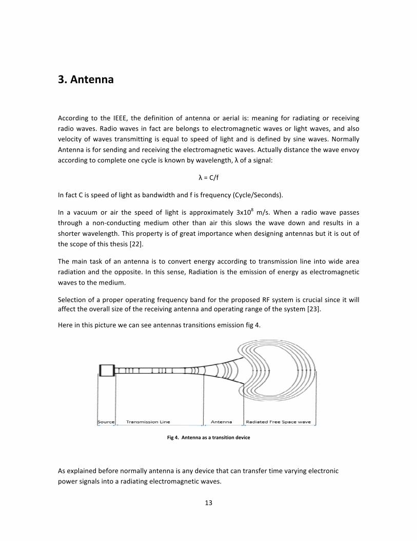
Here in this picture we can see antennas transitions emission fig 4.

Fig 4. Antenna as a transition device

As explained before normally antenna is any device that can transfer time varying electronic power signals into a radiating electromagnetic waves.

14

Fig 5. Basic components of a wireless communication transmitting and receiving terminal

Transmitter in fact is consisting of data source, encoder, modulator, power amplifier, transmission line or waveguide and antenna. On the other hand receiver terminals consist of an antenna, transmission line or waveguide, radio frequency (RF) amplifier, demodulator, decoder and data destination. The antenna behavior is included by transmission line or waveguide and also antenna at the end of communication point link. The main goal of transmitting lines or waveguides is to carry the Radio frequency from transmitter amplifier to the antenna.

Transmission lines or waveguides can always have power loss in the system, which depends on the size and type of design. In fact the loss increases with increasing frequency and length of line or waveguide. That is why many antenna systems have their proper power amplifier as in background such as at indoor space.

In general antennas behave like that of an electronic magnetic radiation which has been accrued when electric charges are accelerated. Distribution of the photons from acceleration depends on energy conservation and charges can be accelerated according to some options. In antennas, the acceleration of a charge experiences usually results from the charge changing direction. Changing direction in such an antenna is caused to charges when they reach the end of wire. For wireless systems, the charges are subjected to sinusoidal varying voltages that continually force a change in the direction of electron travel in response to the changing voltage potential. Electronic magnetic fields are made by radiation which arrived by antenna changes in the exact same way. Therefore resulting in a different EM field at the variation Frequency of impressed voltage with unique amplitude and signal characteristics of that voltage.

3.1 Types of antennas Actually there are four types of antenna according to the applications in WSN world. In this point we will provide some of the most used types of antennas for WSN. We will not enter in details

15

because of this will be out of the scope of this thesis. More information about antenna design and types of antennas can be found in [refs]. So, the most used types of antennas are the following:

3.1.1 Wire Antennas:

The most recognizable antennas are wire ones which are used by TV, cars etc., Wire antennas are included with Dipoles, loops, helical, sleeve dipoles, yagi-‐Uda arrays. Wire antennas specifically include low gain and operates at lower level frequency (HF to UHF). The reason for these characteristics are low cost, simple design and easy to manufacture.

3.1.2 Aperture antennas:

Aperture antennas have a physical opening through which propagating Electromagnetic waves flow [22]. Normally aperture antennas have several wavelengths long in one or some more dimensions. In fact the pattern has a narrow main beam in order to achieve high gain. These kind of antennas are quite useful for aerospace and spacecraft applications because they can be easily flush mounted. Therefore, parabolic reflectors, horn antennas, lense antennas and circular apertures are included.

3.1.3 Array Antennas:

Array antennas are constructed according to individually matrix and radiated. The model of array antennas is defined by amplitude, phase of excitation field on behalf of each source and also geometric spacing of resources. Normally these types of antennas are integrated with Dipoles, Monopoles, waveguides included with slot, open ended antennas and micro strip radiators.

3.1.4 Printed Antennas:

These type of antennas are covered by all of the aforementioned types of antennas, in fact this type of antenna is made with photolithographic methods with feeding fundamental and also this antenna is constructed on a dielectric substrate. Microstrip antennas are relatively inexpensive to manufacture and design because of the simple 2-‐dimensional physical geometry. It is important to remark that the dielectric loading of a microstrip antenna affects both its radiation pattern and impedance bandwidth. As the dielectric constant of the substrate increases, the antenna bandwidth decreases which increases the Q factor of the antenna and therefore decreases the impedance bandwidth.

3.1.5 Chip Antennas:

Chip antennas are a particular type of antenna valued for their small footprint. They are most commonly integrated in circuit boards to radiate high frequency electromagnetic waves. They have a limited range, making them optimal for small devices such as cell phones and WiFi routers. Their most notable difference is their small size. This means they can often be internalized within small electronic devices; they are also inexpensive considering their quality. Chip antennas are the best alternative when a larger-‐sized antenna is impractical.

16

4. Propagation, channel and fading

Propagation and also distribution of signals have been included in some models which are the main part of the tools for designing any fixed broadband wireless communications systems. Propagation is used for some predictability abilities through transmit signal while in transit to the receiver.

In fact the signal is weakened and also changes the form of signals or distorted in particular ways and in this situation receiver must be able to accommodate the changes. Types or model of transmitter and receiver of devices and communications services will be affected by these signals impairment and distortions. The role of propagation modeling in general is to predict system performance with these types of distortions and also to determine whether successfulness of performance to goals and services objectives, which is involved as propagation model is applied to the algorithms and related methods for predict the medial signal level at the receiver in fact in general could be a model of entire transfer function of channel.

Early communication systems were narrowband systems in which median signal level prediction along with some description of signal level variability (fading) statistics were the only models needed to adequately predict system performance [24]. In modern systems higher data rates is achieved by using a wider band of frequencies therefore in such a systems narrowband prediction of signal levels and also fading individually unable to provide enough information for predictably of system performance. Entire transfer functions of channels and related models are substitutes of all modifications the transmitted signal undergoes in process through transmitting and receiving by far these models are included signal level information, signal time dispersion information and in the case of mobile systems, models of Doppler shift distortions arising from the motion of the mobile. Suitably these kinds of models that provide some additional information are called Channel Models. A model is selected by the system designer to be appropriate to the design problem being addressed because these models are invented to generate vital information needed for system performance prediction tasks.

For example, for the preliminary step of dimensioning a Local Multipoint Distribution Service (LMDS) system at 28 GHz, a simple model that predicts the service radius of a hub is all that is required to estimate the number of hubs needed to cover the intended service area [24]. In reality base system fundamental is performed from a comprehensive point to point model might be created whether a path in line of sight is mandatory. So such a model uses the terrain details for database building and also on the useful methods for predicting the availability and qualifications of links with multipath and rain fading situations.

17

Model classifications are included to propagation and channel models in designing and constructing successful communication systems, therefore a huge amount of effort has been devoted on behalf of industrial to developing such models: Theoretical models are a small application just fixed broadband wireless system except probable to use for rain attenuation perfectibility. Empirical Models, at present are the main processes of measurement or on the other hand observations to develop and also performance of signal in areas which have real propagation. Usage of this type of model is for dimensioning Non line of sight (NLOS) point to multipoint systems more regular than other others. Physical Models, this model is just using the physical behavior of electromagnetic (EM) wave propagation. The main function of this task is to predict signal attenuation and also channel response, this type of model actually is design for fixed broadband wireless systems. On the other hand physical models are sometimes called deterministic models as well, because probability of analysis that is applied to the channel modeling therefore channel response characteristics might be divided through deterministic and random process paths.

4.1 Fading and interference ‘Fading’ is a broad term that is applied to a wide range of variations observed in the signal amplitude, phase, and frequency characteristics [24]. Wireless propagation and channel modeling actually are categories are belongs to fading, on the other hand fading characteristic of the channel has very important rules in system performance. In wireless communications, fading is deviation of the attenuation that a carrier-‐modulated telecommunication signal experiences over certain propagation media. The fading may vary with time, geographical position and/or radio frequency, and is often modeled as a random process. A fading channel is a communication channel that experiences fading. In wireless systems, fading May either be due to multipath propagation, referred to as multipath induced fading, or due to shadowing from obstacles affecting the wave propagation, sometimes referred to as shadow fading [25]. Fading classification actually depends on types of information that propagation model by itself can be reliably designed. A fading model is a patch on the main propagation model that describes those observed signals characteristic that the model has not got the ability to predict completely. Fading model elements in fact are function of capabilities that belong to the underlying propagation model. Fading models actually are described impact of physical mechanisms to support current technology of wireless networking in concrete applications such as predicting atmospheric refractivity along a given link path and would require a model that could take into account the temperature, the pressure, and the humidity at all points along the path and also take into account how the gases in the atmosphere respond – clearly an intractable problem with current

18

calculation technology and data sources. Similarly, predicting when rain will cause a fade on a particular microwave link is as difficult as predicting the weather. There is a very important issue in non-‐line of sight (NLOS) systems; these signals are strongly affected by systems in concert examples, when by moving cars and related vehicles. In fact their movement and effect types are not as predictable as traffic flow and should be shown and declared by some statistical methods. All of these categories mentioned above and many others that affect radio distribution are accounted for in the system planning behavior using fading models. The task of fading models for predicting system performance is quiet meaningful. In related design reliability scale that is probable only allow an outage for few ranges of time such as minutes a year, the specific occurrence details of very low probability outage events, here we can declare rain which can be a bit important especially in some climates which have lot of rain. By far setting up transmit power levels are sufficient to achieve an acceptable fade margin Impact system cost as well as the potential for frequency reuse within a system and probable interference in neighbor close node systems. There are some fading models such as Rayleigh, rician and lognormal probability distributions to describe signal amplitude varieties. These models are used in designing mobile and cellular radio systems. For high availability fixed link systems, however, the detailed shape of the low probability tail of the distribution functionality is quite important on that simple, approximate statistical models like those used in mobile communication are normally not sufficient for this goal. In place of concrete models, they have been designed to be better at predicting the occurrence of very low probability events. In NLOS systems currently there is available fading distributions system, in fact it has just happened in low frequency and also customized empirical models of the ‘tail’ that’s why it’s impossible to use for NLOS systems at lower frequencies, as the fading distribution is not available, there is no choice but to make use of Rayleigh, Rician, and lognormal fading models which are familiar with cellular and mobile radio network design. While amplitude of the signal and interference will much different and vary (Fade) with the following statistical distribution then Signal to noise ratio(SNR) and Signal to interference ratio(SIR) values also are vary with time. The percentage of time the SNR and the SIR values are both above the desired thresholds is the link availability. The inverse of link availability is link outage. The threshold point ρth where the performance is acceptable is usually the point where the raw bit error rate (BER) is too high for the error-‐correcting mechanisms to successfully remove essentially all the errors. The threshold will therefore vary as a function of link equipment design. The link outage probability can be written as Pr (outage) =Pr (𝛒 (t) <𝛒th) (1)

𝛒 (t) = !(!)! ! !!(!)

19

The variables S, I, and N are random variables representing the desired signal, the interference, and the noise, respectively. If the probability distribution functions of these random variables are known, then the probability distribution of ρ(t) can be found and the probability of an outage determined. The amplitude of the desired signal S (t) will experience variations or fading that depends on the propagation environment, the link geometry, the antennas used, and the bandwidth of the signal. For fixed broadband systems, the fading can be considered in two general, non-‐exclusive categories: • Line-‐of-‐Sight (LOS) Links. For LOS links, the use of high gain directional antennas provides a degree of multipath rejection, which reduces the short-‐term fading depending on the link path length. In the case of long ( >5 km) microwave paths subject to atmospheric fading in case of the amplitude fading is described by empirical models that have been formulated using a vast collection of link performance data. These distributions are sometimes approximated using Rice or lognormal distributions. By contrast, in the case of short ( <5 km) microwave links in urban areas where rooftop antennas provide significant elevation above the reflection surface, the large angular difference between the LOS direct signal and the reflections allows the antenna gain pattern to successfully suppress the reflections and thus reduce the fading and the time dispersion. The resulting signal envelope can be quite stable for long periods of time. • NLOS Links, The signal amplitudes for links in obstructed non-‐LOS locations will exhibit fading that is similar to fading in mobile or cellular channels. This fading is usually described by a composite density consisting of Rayleigh distributed envelope amplitude fading (‘fast fading’) due to multipath signals and lognormal fading of the mean values. Rayleigh fading models assume that the magnitude of a signal that has passed through such a transmission medium (also called a communications channel) will vary randomly, or fade, according to a Rayleigh distribution. Rayleigh fading is most applicable when there is no dominant propagation along a line of sight between the transmitter and receiver. The fast-‐fading distribution is due to shadowing by propagation environment features that are not accounted for by the propagation model. The necessity for statistical descriptions of shadow fading depends on the capabilities of the propagation model. Multiple fading actually is modeled using many kinds of specific probability distribution to declare variation packet voltage of signal. The models in fact are showed up that the signal is sufficiently narrowed according to the fading is not frequently-‐selective. Even in channels in which the bandwidth of the signal and the nature of the propagation environment result in frequency-‐selective fading, flat fading models such as these can still be used to describe the fading that occurs in time segments (windows or bins) or narrow frequency segments of the overall signal bandwidth [24].

20

4.2 Fading models There is some statistical probability density function (pdfs), so the most important and common models are: • Rayleigh • Rician • Nakagami 4.2.1 Rayleigh In radio systems engineering, the distribution of the flat-‐fading envelope has in the past usually been assumed to be a Rayleigh distribution [26].

Fig 6. Rayleigh-‐distributed vector r

The Rayleigh distribution describes the probability distribution function (PDF) of the magnitude of the resultant vector sum of two independent, Zero mean Gaussian random variables in quadrature, shown in Figure6 asnx(t) ny(t ). By the Central Limit Theorem, the distribution of the sum of a large number of random variables will yield a random variable with a Gaussian distribution regardless of the distributions of the individual random variables in the sum. Even with as few as six randomly phased sinusoids, the envelope of the sum is essentially Rayleigh [27]. From this perspective, when a large number of multipath components are considered, the Rayleigh distribution can be a justifiable choice. Using this geometry, the pdf of the resultant vector can be derived into the following basic form:

Pr(r) = !!!exp !!!

!!! (2)

21

Where δ2is the variance of the Gaussian distributions (both assumed to be the same). It can be shown [27] that the phase of the angle θ is uniformly distributed from 0 to 2π. A plot of the Rayleigh distribution is shown in Figure 11. The median of the distribution is found by finding the value for r for which 50% of the area of the distribution is above and below this value of r:

0.5= Pr r dr = exp !!!

!!!!! (3)

The median is then found as𝑟 = 1.17 2 . In similar way, the mean r and the variance b2 for the Rayleigh distribution can be found by integrating p(r) to yield

ṝ= !!𝜎 = 1.25σ (5)

b2=𝜎2(2-‐!!) (6)

The ratio of the mean to the variance of the Rayleigh distribution is

ṝ!!= !.!"

!(!!!!)= 2.91/σ (7)

Where X has many distribution px(x) (Rayleigh in this case), the distribution for y (Power) is given by [28]

PY (y)=!"( !/!)!!"(! !

!

!! ! for y ≽ 0 (8)

22

Fig 7. Rayleigh and Rician distribution pdfs for several values of k factor

For analyzing the SNR or SIR, it is often more convenient to describe the distribution of the instantaneous power in the fading signal rather than its envelope voltage. The pdf of the instantaneous power can be found by using the probability function conversion. For the function

Y=cX2 (9)

The resulting pdf for the instantaneous power s(t)=|r(t)|2 is then:

Ps(s) = !!! !exp − !

!! ! (10)

A Rayleigh distribution is the pdf that describes the envelope of two Gaussian-‐distributed variants in quadrature. However, there are circumstances when a single ray will be much stronger than the others. This occurs close to the transmitter in LOS conditions when the ray received directly from the ransmitter is stronger than the others.It can also occur in some NLOS receive sites if some characteristic of the propagation environment causes a single ray to be much higher in amplitude than the others. A receive location at the peak of the diffraction field of a corner diffraction source could result in a single strong ray compared to the others being received. The distribution of the amplitudes of such a signal is best modeled with the Rician distribution.

23

4.2.2 Rician fading

Rician fading is a stochastic model for radio propagation also this type of model is caused by partial cancellation of radio signal which is done according to task by itself. Rician fading signals at the receiver side is arrived in many different paths which is sometimes called multiple interference. Therefore when one of the paths’ normal line of sight is much stronger that the others, the rician fading will be invented. Here it should be taken into account that Rayleigh fading is one of the most important models for stochastic fading when line of sight signal will not exist and also amplitude gain is characterized by a Rayleigh distribution. When a single strong constant amplitude component is included in the sum along with a number of weaker components, the distribution of the sum can be described by the Rician distribution [29].

pr(r) = !! ! exp (

! !!!!!!!! ! + I0( !!!! !) (11)

Where Ac is the amplitude of the constant amplitude sine wave component𝜎 ! is the variance of the Gaussian noise, and I0 is the modified Bessel function of the first kind and zero order. When

Ac is small compared to 𝜎 ! , the pdf p(r) is essentially Rayleigh. Several examples of the Rician pdf with different k factors are plotted in Figure Where 4.14. When Ac is zero, (11) is identically the same as the Rayleigh distribution. The Rayleigh distribution therefore can be viewed as simply a

special case of the Rician distribution. When Acis large compared to 𝜎 ! , the pdf is essentially the same as a Gaussian distribution with a mean value of Ac. The ratio of the constant amplitude component to the variance is called the Rician k factor of the distribution and is calculated as follows:

K= ( !!!!" !) (12)

As with the Rayleigh distribution, it is useful to have the pdf of the instantaneous power s (t) =|r (t)|2, which is found in the same way as described above using (4.59):

Ps (s) = !!" ! exp (

!!!!!!" ! + I0(

! !! !! ! ) (13)

The average power is given by the sum of the powers in the constant amplitude component and

the variable component, E[s] = 𝐴 !!+2𝜎 ! . The cumulative distribution function (CDF) for the

Rician distribution is given by F(r<b) =1-‐Q (!!

!,!!) (14)

Where Q (a, b) is the Marcum Q function.

24

4.2.3 Nakagami distribution The third distribution considered here for modeling the multipath-‐induced voltage envelope variations represented by the random variable r is the Nakagami or Nakagami-‐m distribution[45]. Unlike the Rayleigh and Rician distributions, which are derived from real physical quantities in nature (Gaussian noise and the sine wave), the Nakagami distribution is a mathematical construction with no physical foundation. The Nakagami distribution is given by Pr(r) = !

!(!)!!

mr2m-‐1exp !!!𝑟 ! r≽0, m≽0.5 (15)

Where m is the parameter that controls the basic shape of the distribution and Ω is the mean square value. The function Γ (m) is the Gamma function defined by Γ(x) = t !

! n-‐1e-‐t dt x>0 (16)

Tabulations of the gamma function can be found in mathematical tables. Also, recursive relationships and polynomial approximations are available. For the special case of x=0.5 Γ(x) =

Γ𝑥 = ¶ Using this value in F(r < b) = 1 – Q (!"

!, !!) (17)

taking m as 0.5, becomes the Gaussian distribution for x>0.Form = 1.0, it becomes the Rayleigh distribution with Ω=�2. Compared to the Rayleigh and Rician distributions, the Nakagami distribution is more flexible in creating a wide range of pdf shapes and is to some extent more mathematically tractable than the Rician distribution because the modified Bessel function is absent. However, the physical rationalization of the Rician distribution is satisfying when it is tied to a physical approach to modeling communication channels. The artificial mathematical construction of the Nakagami distribution is a useful curve-‐fit to experimental data. It can be the most convenient distribution to use in many cases.

25

Conclusion In the first chapter, we focused on Wireless Sensor network (WSN) IEEE 802.15.4 theory in short distance telecommunication technology. Actually Some benefits of WSN are discussed as flexibility, fault tolerance, high sensing fidelity, low energy consumption, low-‐cost and the most important of all easy developing. Therefore, WSN devices have the ability to be extremely small, low powered programmable computing, multiple parameter sensing, and better wireless communication in short ranges. WSN equipment arranged based on Sensor nodes and master nodes, sensor nodes tasks are collecting data and communication with other the closest nodes coming with preferring algorithm and Finally transferring data to the master nodes. Master node, normally called coordinator has a rule as communicating with sensors, save data and passes them through the gateway from inside transaction to outside database. Communication methods in WSN are discussing in two ways: first, as a single hop communication and second as multi-‐hop communication depends on which algorithm can have the lowest cost in such a network. On behalf of this concept, we have investigated how to achieve the best algorithm to decrease the power consumption and increase the network life cycle in person area network (PAN). Related to WSN standard and our idea, we analyzed how to create a new algorithm to obtain even better results in this technology. In this case, data path routing was measuring accurately in two fundamental OSI layers included MAC and network layer to achieve minimum energy consumption and maximum network life cycle. In addition, we have concentrated in hardware design and their behavior in WSN such as; antenna, transceiver, sensors, power, memory and processors. In the next chapter, we manipulate this hardware according to the IEEE 802.15.4 standard to construct the basement of WSN and readiness for the network layer, which is involved in our routing protocol. As we mentioned, depending on our idea we will focus on decreasing battery consumption and increasing network life cycle in WSN to use in various applications.

References: [1] Vivek Mhatre, Catherine Rosenberg “Homogeneous vs Heterogeneous Clustered Sensor Networks: A Comparative Study “School of Electrical and Computer Eng., Purdue University, West Lafayette, West Lafayette, IN 47907-1285. [2] Ankita, “ International Journal of Advanced Research in Computer Science and Software Engineering “ Scholar, Department of Computer Science and Applications Kurukshetra University, Kurukshetra, India, Volume 4, Issue 4, April 2014. [3] Siddharth Ramesh “A Protocol Architecture for Wireless Sensor Networks “School of Computing, University of Utah, Salt Lake City, UT 84112. [4] Arati Manjeshwar , Dharma P. Agrawal “TEEN: A routing protocol for enhanced efficiency in wireless sensor networks (2001)” Center for Distributed and Mobile Computing, ECECS Department, University of Cincinnati, Cincinati,OH 45221-0030, 2001 [5] C. Intanagonwiwat, R. Govindan, D. Estrin, Directed diffusion: a scalable and robust communication paradigm for sensor networks, Proceedings of the ACM Mobi-Com’00, Boston, MA, 2000, pp. 56–67. [6] I.F. Akyildiz, W. Su, Y. Sankarasubramaniam, E. Cayirci “Wireless sensor networks: a survey” Broadband and Wireless Networking Laboratory, School of Electrical and Computer Engineering, Georgia Institute of Technology, Atlanta, GA 30332, USA, Volume 38, Issue 4, 15 March 2002, Pages 393–422

26

[7] E. Shih, S. Cho, N. Ickes, R. Min, A. Sinha, A. Wang, A. Chandrakasan, Physical layer driven protocol and algorithm design for energy-efficient wireless sensor networks, Proceedings of ACM MobiCom’01, Rome, Italy, July 2001, pp. 272–286. [8] E.M. Petriu, N.D. Georganas, D.C. Petriu, D. Makrakis, V.Z. Groza, Sensor-based information appliances, IEEE Instrumentation and Measurement Magazine (December 2000) 31–35. [9] A. Cerpa, J. Elson, M. Hamilton, J. Zhao, Habitat monitoring: application driver for wireless communications technology, ACM SIGCOMM’2000, Costa Rica, April 2001. [10] G.J. Pottie, W.J. Kaiser, Wireless integrated network sensors, Communications of the ACM 43 (5) (2000) 551– 558. [11] S. Vardhan, M. Wilczynski, G. Pottie, W.J. Kaiser, Wireless integrated network sensors (WINS): distributed in situ sensing for mission and flight systems, IEEE Aerospace Conference, Vol. 7, 2000, pp. 459–463. [12] J.M. Rabaey, M.J. Ammer, J.L. da Silva Jr., D. Patel, S. Roundy, PicoRadio supports ad hoc ultra-low power wireless networking, IEEE Computer Magazine (2000) 42–48. [13] A. Perrig, R. Szewczyk, V. Wen, D. Culler, J.D. Tygar, “SPINS: security protocols for sensor networks”, Proceedings of ACM MobiCom’01, Rome, Italy, 2001, pp. 189–199. [14] J.M. Kahn, R.H. Katz, K.S.J. Pister, “Next century challenges: mobile networking for smart dust”, Proceedings of the ACM MobiCom’99, Washington, USA, 1999, pp. 271–278. [15] Mikhaylov, K. ; RF Media Lab., Univ. of Oulu, Ylivieska, Finland ; Tervonen, J. “Optimization of microcontroller hardware parameters for Wireless Sensor Network node power consumption and lifetime improvement “Ultra Modern Telecommunications and Control Systems and Workshops (ICUMT), 2010 International Congress on, Oct. 2010, pp. 1150 – 1156 [16] Denis C. Daly and Anantha P. Chandrakasan “An Energy Efficient OOK Transceiver for Wireless Sensor Networks” Microsystems Technology Laboratories, Massachusetts Institute of Technology Cambridge, MA 02139, USA [17] http://wsn.oversigma.com/wiki/index.php?title=Radio_Transceivers [18] Holger Karl and Andreas Willig, “Protocols and Architectures for Wireless Sensor Networks” ISBN: 0-470-09510-5, 2005 [19] http://www.eecs.harvard.edu/~konrad/projects/shimmer/references/tmote-sky-datasheet.pdf [20] Andy Nisbet1 and Simon Dobson, ” A systems architecture for sensor networks based on hardware/software co-design “Manchester Metropolitan University, Manchester UK, Department of Computer Science, University College, Dublin IE, 2004 [21] http://en.wikipedia.org/wiki/Sensor_node [22] Griogair W.M. Whyte, “Antennas for Wireless Sensor Network Applications” Department of Electrical and Electronic Engineering, Faculty of Engineering, University of Glasgow, 2008 [23] Rajiv Dahiya, A. K. Arora and V. R. Singh, “Analysis of Wireless Sensor Networks with Energy Harvesting Capabilities of Transmitter and Receiver Antenna” Research Scholar, Manav Rachna International University, Faridabad, International Journal of Engineering and Innovative Technology (IJEIT), Volume 3, Issue 12, June 2014 [24] Harry R. Anderson, Ph.D., P.E. “fixed broadband wireless system design” consulting engineer usa ” consulting engineer usa, 2003

[25] https://www.princeton.edu/~achaney/tmve/wiki100k/docs/Fading.html [26] W.C. Jakes. Microwave Mobile Communications. IEEE Press: Piscataway, New Jersey. 1994 (re-published). Chapter 1. [27] M. Schwartz, W.R. Bennett, and S. Stein. Communication Systems and Techniques. NewYork: McGraw-Hill, 1966. page 329. [28] P.Z. Peebles. Probability, Random Variables, and Random Signal Principles. New York: McGraw-Hill. 1980. page 72. [29] S.O. Rice, “Statistical properties of a sine wave plus random noise,” Bell System Technical. Journal, vol. 27, no. 1, pp. 109–127, January 1948.

27

Chapter 2. The Physical Layer for wireless sensor networks based on IEEE802.15.4

28

1. Introduction

The theoretical origin of communications between two points using electromagnetic waves propagating through space can be traced to James Maxwell’s treatise on electromagnetism, published in 1873, and later to the experimental laboratory work of Heinrich Hertz, who in 1888 produced the first radio wave communication. Following hertz’s developments at the end of the nineteenth century, several researchers in various countries were experimenting with controlled excitation and propagation of such waves. The first transmitters were of the ‘spark-‐gap’ type. A spark-‐gap transmitter essentially worked by producing a large energy impulse into a resonant antenna by way of a voltage spark across a gap. The resulting wave at the resonant frequency of the antenna would propagate in all directions with the intention that a corresponding signal current would be induced in the antenna apparatus of the desired receiving stations for detection there.

Early researchers include Marconi, who while working in England in 1896 demonstrated communications across 16km using a spark-‐gap transmitter, and Reginald Fassenden, who while working in the United States achieved the first modulated continuous wave transmission.

All wireless communication systems can be modeled using a few basic blocks as shown in Figure 1. Communication starts with an information source that can be audio, video, data as e-‐mail, image files or other data in many forms. The transmitter converts the information into a signaling format (coding and modulation) and amplifies it to a power level that is needed to achieve successful reception at the receiver. The transmitting antenna converts the transmitter’s power to electromagnetic waves that propagate in the directions determined by the design and orientation of the antenna. The propagation channel shown in figure 1 is not a physical device but rather represents the attenuation, variations, and any other distortions that affect the EM waves to propagate from the transmitting antenna to the receiving antenna.

Fig 1. Block diagram of a basic wireless communication system

29

It was not so long ago that there was a serious debate over whether or not wireless communications in general and in particular the use of wireless sensor networks was a technology suitable for industrial/technical/biomedical applications. The increased adoption of wireless sensors across industry is basically due to solid and practical reasons. Chief among these reasons is ease of implementation (no long cable runs), ability to operate in harsh environments, easy troubleshooting and repair, and high levels of performance [1].

Some of the most important advances that have been developed in the field of wireless sensor networks (WSNs) are directly correlated with the advances in semiconductor, networking and material science technologies. All these technologies are driving the ubiquitous deployment of large-‐scale wireless sensor networks (WSNs). Together, these technologies have combined to enable a new generation of WSNs that differ greatly from wireless networks developed and deployed as recently as 5 to 10 years ago. Today’s state-‐of-‐the-‐art WSNs have lower deployment and maintenance costs, last longer and are more rugged. They are finding their way into numerous applications in our homes, work places and beyond, bringing new sources of information, control and convenience to our personal and professional lives. To understand the tradeoffs in today’s WSNs, it is helpful to briefly examine their history. Like many advanced technologies, the origin of WSNs can be seen in military and heavy industrial applications, far removed from the light industrial and consumer WSN applications that are prevalent today. The first wireless network that bore any real resemblance to a modern WSN is the Sound Surveillance System (SOSUS), developed by the United States Military in the 1950s to detect and track Soviet submarines. This network used submerged acoustic sensors – hydrophones – distributed in the Atlantic and Pacific oceans. This sensing technology is still in service today, albeit serving more peaceful functions of monitoring undersea wildlife and volcanic activity. [2]

2. Technical Standards Most wireless systems in general, and WSN is not an exception, use technology and engineering methods that comply with a minimum regulatory framework but otherwise are proprietary methods that have been developed to achieve an advantage over their commercial competition. One of the most important institutions for the electronic standard definition is the IEEE, the Institute of Electrical and Electronics Engineers, founded in 1884 as the American institute of electrical engineers, AIEE. The IEEE was formed in 1963 when the AIEE merged with the institute of radio engineers, IRE. The IEEE is an organization composed of engineers, scientists and students. It is best known for developing standards for the computer and electronics industry [3]. In particular we can highlight in the IEEE 802 standards for local area networks (LAN). Two different subgroups born from IEEE 802: Those that define wired LANs, as Ethernet (802.3), Token Ring (802.5) and Token Bus (802.4) and those that define wireless LANs, as WiFi (802.11), WIMAX (802.16), and a special case for the personal and sensing communication defined by 802.15. Among them we have the lower layers of Bluetooth (802.15.1) and Zigbee (802.15.4). The IEEEE only defines the first two layers; it is the physical and data link layers. This is usually known as medium access control (MAC) layer.

30

We focus this thesis on the study and development of protocols and minimization of power consumption of WSN based on 802.15.4. In future chapters we will define some of the upper layers, but in this chapter we are going to define the implemented physical layer, following the IEEE standard.

Initially, the IEEE 802.15.4 standards were defined to cover information over relatively short distances. However, the increase of the technology and the different applications made that 802.15.4 would be used for wide sensor area network. The distance among sensors (the coverage distance) was about 5 to 30 meters, but implementing some routing protocols, the coverage area could be more than km.

2.1 Devices and transceivers

The device used in this thesis implements transceivers from Texas instruments. These transceivers are the well-‐known CC2420 and CC2520, the last one is just an upgrade of the first one, but basically both of them act using the same methodology. Both chips work at 2.4 GHz unlicensed ISM band. It includes a digital direct sequence spread spectrum (DSSS) baseband modem providing a spreading gain of 9 dB and an effective data rate of 250 kbps. These devices provides extensive hardware support for packet handing, data buffering, burst transmissions, data encryption, data authentication, clear channel assessment, link quality indication and packet timing information. These features reduce the software load of the host controller, minimizing the power of this and then decreasing the cost and the power consumption. The configuration interface and the FIFOs buffers for transmission and reception are accessed via a synchronous serial communication: The SPI interface.

The microcontroller used to connect with our transceiver is the well-‐known MSP430F1611 [4], from Texas Instruments. This device is based on a 16-‐bit RISC microprocessor, specially designed for ultralow power applications. In particular, it has two SPI interfaces; one of them is used to interconnect the microcontroller with the CC2X20 transceiver.

The WSN alone cannot transmit the collected data on its own. It is necessary to implement a gateway to encapsulate the information and store all the data in a database to be studied and analyzed. This performance is done by another device: The CC3200. This device, on one way is connected to the WSN thru the above commented CC2520. The connection with the CC2520 is thru an SPI serial communication interface, which connects the Launchpad board with a daughter board that implements this transceiver. On the other way, the CC3200 can connect to a WiFi network to transmit the data to an external database. The CC3200 is a 32-‐bit ARM [5] core based processor that implements a simple link WiFi transceiver, being only necessary to implement the antenna connection.

31

2.2 Main characteristics of the physical layer

The IEEE 802.15.4 belongs to the Low-‐Rate Wireless Personal Area Networks (LR-‐WPAN) group of the IEEE. A LR-‐WPAN is a simple, low-‐cost communication network that allows wireless connectivity in applications with limited power and relaxed throughput requirements. If we could highlight the major properties to these kinds of networks we will point to: (i) ease of installation, (ii) reliable data transfer, (iii) short-‐range operation, (iv) extremely low cost, and (v) a reasonable battery life, while maintaining a simple and flexible protocol.

Two different device types can participate in this network: a full functional device or FFD and a reduced functional device or RFD. The FFD can operate in three modes serving as a personal area network coordinator, a router or a device. A FFD can talk to RFDs or other FFDs, while an RFD can talk only to an FFD [6].

The coordinator is a particular case of a FFD and is responsible for overall network management. Each network has exactly one coordinator. The coordinator performs the following functions:

1. Select the channel to be used by the network 2. Starts the network 3. Assigns how addresses are allocated to nodes or routers 4. Permits other devices to join or leave the network 5. Holds a list of neighbors and routers 6. Transfers application packets.

The Router is another type of FFD. A router is used in tree and mesh topologies to expand network coverage. The function or a router is to find the best route to the destination over which to transfer a message. A router performs all functions similar to a coordinator except the establishing of a network. The End device can be an RFD. An RFD operates within a limited set of the IEEE 802.15.4 MAC layer, enabling it to consume less power. The end device must connect to a router or coordinator to transmit the collected data [7].

An RFD is intended for applications that are extremely simple, such as a light switch or a passive infrared sensor. They do not have the need to send large amounts of data and may only associate with a single FFD at a time. Consequently, the RFD can be implemented using minimal resources and memory capacity. It usually operates at low duty cycle power, meaning it consumes power only while transmitting information.

A WSN can include as many RFD as it would be necessary but it must include at least one FFD.

One of the important concepts to be taken into account is the coverage area. The coverage area is the longest distance where you can place a node (an FFD or a RFD) without extremely large loose of packets. There is not a perfect definition of coverage area for WSN. A well-‐defined coverage area does not exist in fact for wireless media because propagation characteristics are dynamic and

32

uncertain. Small changes in position or direction may result in drastic differences in the signal strength or quality of the communication link. These effects occur whether a device is stationary or mobile as moving objects may impact station-‐to-‐station propagation.

The PHY layer provides two services: The PHY data service and the PHY management service interfacing to the physical layer management entity (PLME). The PHY data service enables the transmission and reception of the PHY protocol data units across the physical radio channel [6].

2.2.1 Data Packet structure

The LR-‐WPAN standard allows the optional use of a superframe structure. The format of the superframe is defined by the coordinator and is something similar to that shown at figure 2. The superframe is bounded by network beacons, sent by the coordinator and is usually divided (if we follow the standard) in 16 equally slots. The beacon frame is transmitted in the first slot of each superframe. If a coordinator does not wish to use a superframe structure, it may turn off the beacon transmissions. The beacons are just used to synchronize the attached devices, to identify the PAN, and to describe the structure of the superframes. Any device wishing to communicate during this contention access period between two beacons should compete with other devices using a slotted CSMA-‐CA mechanism. Moreover, all transactions must be completed by the time of the next network beacon.

Fig 2. Superframe structure with GTSs

For low-‐latency applications or applications requiring specific data bandwidth, the PAN coordinator may dedicate portions of the active superframe to that application. These portions are called guaranteed time slots (GTSs). The GTSs form the contention-‐free period (CFP), which always

33

appears at the end of the active superframe starting at a slot boundary immediately following the CAP, as shown in Figure 3. The PAN coordinator may allocate up to seven of these GTSs, and a GTS may occupy more than one slot period. However, a sufficient portion of the CAP shall remain for contention-‐based access of other networked devices or new devices wishing to join the network. All contention-‐based transactions shall be complete before the CFP begins. Also each device transmitting in a GTS shall ensure that its transaction is complete before the time of the next GTS or the end of the CFP. More information on the superframe structure can be found in 7.5.1.1.

Fig 3. Superframe structure without GTSs

It is important to remark that the data packet structure used in this thesis is not based on this superframe structure. The contention free period covers all the time[6].

2. 3 Data Transfer Model Three types of data transfer transactions exist. The first one is the data transfer to a coordinator in which a device transmits the data. The second transaction is the data transfer from a coordinator in which the device receives the data. The third transaction is the data transfer between two peer devices. In star topology only two of these transactions are used, because data may be exchanged only between the coordinator and a device. In a peer-‐to-‐peer topology data may be exchanged between any two devices on the network; consequently all three transactions may be used in this topology. The mechanisms for each transfer type depend on whether the network supports the transmission of beacons. A beacon-‐enabled network is used for supporting low-‐latency devices, such as PC peripherals. If the network does not need to support such devices, it can elect not to use the beacon for normal transfers. However, the beacon is still required for network association [6].

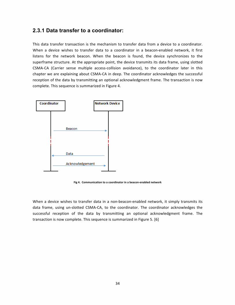
34

2.3.1 Data transfer to a coordinator: This data transfer transaction is the mechanism to transfer data from a device to a coordinator. When a device wishes to transfer data to a coordinator in a beacon-‐enabled network, it first listens for the network beacon. When the beacon is found, the device synchronizes to the superframe structure. At the appropriate point, the device transmits its data frame, using slotted CSMA-‐CA (Carrier sense multiple access-‐collision avoidance), to the coordinator later in this chapter we are explaining about CSMA-‐CA in deep. The coordinator acknowledges the successful reception of the data by transmitting an optional acknowledgment frame. The transaction is now complete. This sequence is summarized in Figure 4.

Fig 4. Communication to a coordinator in a beacon-‐enabled network

When a device wishes to transfer data in a non-‐beacon-‐enabled network, it simply transmits its data frame, using un-‐slotted CSMA-‐CA, to the coordinator. The coordinator acknowledges the successful reception of the data by transmitting an optional acknowledgment frame. The transaction is now complete. This sequence is summarized in Figure 5. [6]

35

Fig 5. Communication to a coordinator in a nonbeacon-‐enabled network

2.3.2 Data transfer from a coordinator: This data transfer transaction is the mechanism for transferring data from a coordinator to a device. When the coordinator wishes to transfer data to a device in a beacon-‐enabled network, it indicates in the network beacon that the data message is pending. The device periodically listens to the network beacon and, if a message is pending, transmits a MAC command requesting the data, using slotted CSMA-‐CA. The coordinator acknowledges the successful reception of the data request by transmitting an optional acknowledgment frame. The pending data frame is then sent using slotted CSMA-‐CA. The device acknowledges the successful reception of the data by transmitting an acknowledgment frame. The transaction is now complete. Upon receiving the acknowledgement, the message is removed from the list of pending messages in the beacon. This sequence is summarized in Figure 6.

Fig 6. Communication from a coordinator a beacon-‐enabled network

36

When a coordinator wishes to transfer data to a device in a non-‐beacon-‐enabled network, it stores the data for the appropriate device to make contact and request the data. A device may make contact by transmitting a MAC command requesting the data, using un-‐slotted CSMA-‐CA, to its coordinator at an application-‐defined rate. The coordinator acknowledges the successful reception of the data request by transmitting an acknowledgment frame. If data is pending, the coordinator transmits the data frame, using un-‐slotted CSMA-‐CA, to the device. If data are not pending, the coordinator transmits a data frame with a zero-‐length payload to indicate that no data were pending. The device acknowledges the successful reception of the data by transmitting an acknowledgment frame. The transaction is complete. This sequence is summarized in Figure 7.

Fig 7. Communication from a coordinator in a nonbeacon-‐enabled network

According to the aforementioned explanation in our case study we focus and develop on non-‐beacon data transmission and this process is automatically done by proper transceivers which are chosen as CC2x20 series, in this model we put the node as a next hop address in the payload and payload according the each characteristic of hex code select its next hope and established communication, so later on in this chapter we will explain about this transceiver in brief. [6]

2.4 Frame Structure As explained above, the thesis is just focusing on non-‐beacon data transmission for this reason in this section we are going to explain non-‐beacon frame structure and its behavior in brief. The frame structures have been designed to keep the complexity to a minimum while at the same time making them sufficiently robust for transmission on a noisy channel. Each successive protocol

37

layer adds to the structure with layer-‐specific headers and footers [6]. The LR-‐WPAN defines three frame structures:

1. A data frame, used for all transfers of data 2. An acknowledgment frame, used for confirming successful frame reception 3. A MAC command frame, used for handling all MAC peer entity control transfers

The structure of each of the three frame types (in non-‐beacon case) is described in 2.4.1 through 2.4.4 the diagrams in these subclasses illustrate the fields that are added by each layer of the protocol. The packet structure illustrated below the PHY represents the bits that are actually transmitted on the physical medium.

2.4.1 Data frame Figure 8 shows the structure of the data frame, which originates from the upper layers. The data payload is passed to the MAC sublayer and is referred to as the MAC service data unit (MSDU). The MSDU is prefixed with a MAC header (MHR) and appended with MAC footer (MFR). The MHR contains the frame control, sequence number, and addressing information fields. The MFR is composed of a 16 bit frame check sequence (FCS). The MHR, MSDU, and MFR together form the MAC protocol data unit frame, (i.e., MPDU). The MPDU is passed to the PHY as the PHY data frame payload, (i.e., PSDU). The PSDU is prefixed with an SHR, containing the preamble sequence and the start of frame delimiter (SFD) fields, and a physical header (PHR) containing the length of the PSDU in octets. The preamble sequence and the data SFD enable the receiver to achieve symbol synchronization. The SHR, PHR, and PSDU together form the PHY data packet, (i.e., PPDU). [6]

Fig 8. Schematic view of the data frame

2.4.2 Acknowledgment frame Figure 9 shows the structure of the acknowledgment frame, which originates from the MAC sublayer. The MAC acknowledgment frame is constructed from an MHR and an MFR. The MHR contains the MAC frame control and data sequence number fields. The MFR is composed of a 16 bit FCS. The MHR and MFR together form the MAC acknowledgment frame (i.e., MPDU).

38

The MPDU is passed to the PHY as the PHY acknowledgment frame payload, (i.e., PSDU). The PSDU is prefixed with the SHR, containing the preamble sequence and SFD fields, and the PHR containing the length of the PSDU in octets. The SHR, PHR, and PSDU together form the PHY acknowledgment packet, (i.e., PPDU). [6]

Fig 9. Schematic view of the acknowledgment frame

2.3.3 MAC command frame Figure 10 shows the structure of the MAC command frame, which originates from the MAC sublayer. The MSDU contains the command type field and command specific data, called the command payload. The MSDU is prefixed with an MHR and appended with an MFR. The MHR contains the MAC frame control, data sequence number, and addressing information fields. The MFR contains a 16 bit FCS. The MHR, MSDU, and MFR together form the MAC command frame, (i.e., MPDU).

Fig 10. Schematic view of the MAC command frame

The MPDU is then passed to the PHY as the PHY command frame payload, (i.e., PSDU). The PSDU is prefixed with an SHR, containing the preamble sequence and SFD fields, and a PHR containing the length of the PSDU in octets. The preamble sequence enables the receiver to achieve symbol

39

synchronization. The SHR, PHR, and PSDU together form the PHY command packet, (i.e., PPDU). [6]

2.4.4 Robustness The LR-‐WPAN employs various mechanisms to ensure robustness in the data transmission. These mechanisms are the CSMA-‐CA mechanism, frame acknowledgment, and data verification. [6]

3 CSMA-‐CA mechanisms The CSMA-‐CA algorithm shall be used before the transmission of data or MAC command frames transmitted within the CAP, unless the frame can be quickly transmitted following the acknowledgment of a data request command. The CSMA-‐CA algorithm shall not be used for the transmission of beacon frames, acknowledgment frames, or data frames transmitted in the CFP. If beacons are being used in the PAN, the MAC sublayer shall employ the slotted version of the CSMA-‐CA algorithm for transmissions in the CAP of the superframe. Conversely, if beacons are not being used in the PAN or if a beacon could not be located in a beacon-‐enabled PAN, the MAC sublayer shall transmit using the un-‐slotted version of the CSMA-‐CA algorithm. In both cases, the algorithm is implemented using units of time called backoff periods, where one backoff period shall be equal to a UnitBackoffPeriod symbols. In slotted CSMA-‐CA, the backoff period boundaries of every device in the PAN shall be aligned with the superframe slot boundaries of the PAN coordinator, i.e., the start of the first backoff period of each device is aligned with the start of the beacon transmission. In slotted CSMA-‐CA, the MAC sublayer shall ensure that the PHY commences all of its transmissions on the boundary of a backoff period. In un-‐slotted CSMA-‐CA, the backoff periods of one device are not related in time to the backoff periods of any other device in the PAN. Each device shall maintain three variables for each transmission attempt: NB, CW and BE. NB is the number of times the CSMA-‐CA algorithm was required to backoff while attempting the current transmission; this value shall be initialized to 0 before each new transmission attempt. CW is the contention window length, defining the number of backoff periods that need to be clear of channel activity before the transmission can commence; this value shall be initialized to 2 before each transmission attempt and reset to 2 each time the channel is assessed to be busy. The CW variable is only used for slotted CSMA-‐CA. BE is the backoff exponent, which is related to how many backoff periods a device shall wait before attempting to assess a channel. In un-‐slotted systems, or slotted systems with macBattLifeExt set to FALSE, BE shall be initialized to the value of macMinBE. In slotted systems with macBattLifeExt set to TRUE, this value shall be initialized to the lesser of 2 and the value of macMinBE. Note that if macMinBE is set to 0, collision avoidance will be disabled during the first iteration of this algorithm. Although the receiver of the device is enabled during the channel assessment portion of this algorithm, the device shall discard any frames received during this time.

40

Figure 11 illustrates the steps of the CSMA-‐CA algorithm. When using slotted CSMA-‐CA, the MAC sublayer shall first initialize NB, CW, and BE and then locate the boundary of the next backoff period [Step (1)]. For un-‐slotted CSMA-‐CA, the MAC sublayer shall initialize NB and BE and then proceed directly to step (2). The MAC sublayer shall delay for a random number of complete backoff periods in the range 0 to 2BE – 1 [step (2)] and then request that the PHY perform a CCA [step (3)]. In a slotted CSMA-‐CA system, the CCA shall start on a backoff period boundary. In an un-‐slotted CSMA-‐CA system, the CCA shall start immediately. In a slotted CSMA-‐CA system with the battery life extension subfield set to 0, the MAC sublayer shall ensure that, after the random backoff, the remaining CSMA-‐CA operations can be undertaken and the entire transaction can be transmitted before the end of the CAP. If the number of backoff periods is greater than the remaining number of backoff periods in the CAP, the MAC sublayer shall pause the backoff countdown at the end of the CAP and resume it at the start of the CAP in the next superframe. If the number of backoff periods is less than or equal to the remaining number of backoff periods in the CAP, the MAC sublayer shall apply its backoff delay and then evaluate whether it can proceed. The MAC sublayer shall proceed if the remaining CSMA-‐CA algorithm steps (i.e., two CCA analyses), the frame transmission, and any acknowledgment can be completed before the end of the CAP. If the MAC sublayer can proceed, it shall request that the PHY perform the CCA in the current superframe. If the MAC sublayer cannot proceed, it shall wait until the start of the CAP in the next superframe and repeat the evaluation. In a slotted CSMA-‐CA system with the battery life extension subfield set to 1, the MAC sublayer shall ensure that, after the random backoff, the remaining CSMA-‐CA operations can be undertaken and the entire transaction can be transmitted before the end of the CAP. The backoff countdown shall only occur during the first six full backoff periods after the end of the beacon’s IFS period. The MAC sublayer shall proceed if the remaining CSMA-‐CA algorithm steps (two CCA analyses), the frame transmission, and any acknowledgment can be completed before the end of the CAP, and the frame transmission will start in one of the first six full backoff periods after the beacon’s IFS period. If the MAC sublayer can proceed, it shall request that the PHY perform the CCA in the current superframe. If the MAC sublayer cannot proceed, it shall wait until the start of the CAP in the next superframe and repeat the evaluation. If the channel is assessed to be busy [Step (4)], the MAC sublayer shall increment both NB and BE by one, ensuring that BE shall be no more than aMaxBE. The MAC sublayer in a slotted CSMA-‐CA system shall also reset CW to 2. If the value of NB is less than or equal to macMaxCSMABackoffs, the CSMA-‐CA algorithm shall return to step (2). If the value of NB is greater than macMaxCSMABackoffs, the CSMA-‐CA algorithm shall terminate with a Channel Access Failure status. If the channel is assessed to be idle [Step (5)], the MAC sublayer in a slotted CSMA-‐CA system shall ensure that the contention window has expired before commencing transmission. To do this, the MAC sublayer shall first decrement CW by one and then determine whether it is equal to 0. If it is

41

not equal to 0, the CSMA-‐CA algorithm shall return to step (3). If it is equal to 0, the MAC sublayer shall begin transmission of the frame on the boundary of the next backoff period. If the channel is assessed to be idle in an un-‐slotted CSMA-‐CA system, the MAC sublayer shall begin transmission of the frame immediately. [6]

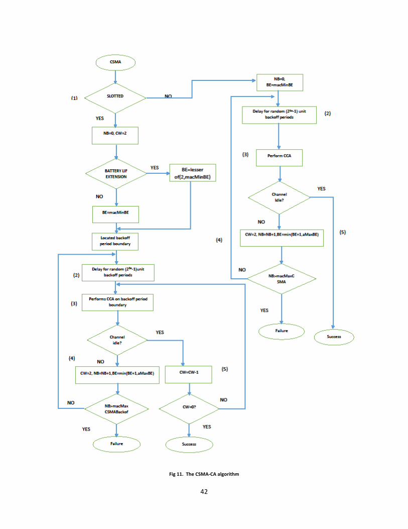
42

Fig 11. The CSMA-‐CA algorithm

43

4 Transceivers used in this thesis In chapter one, we have discussed the characteristics of each of the devices which are used in this thesis in order to have proper results. Also transceivers were pointed out as a device that to send and receive the frames over antenna. The transceivers, which we are using here cc2x20 series belongs to Texas instrument. As mentioned, both types of transceivers are used cc2420 and cc2520 of which cc2520 is the updated version of cc2420. Both of them are following the same rule in this project and the second one cc2520 has the same fundamental as cc2420.

4.1 CC2420

Chipcon AS, a leading provider of high performance, low power, low data rate RF-‐ICs announces the release of the CC2420, the industry’s first 2.4 GHz IEEE 802.15.4 compliant RF Transceiver. Once again, Chipcon confirms its leading position by being the very first company to officially launch a commercially available RF-‐IC that complies with the IEEE 802.15.4 standard and even exceeds its requirements. The CC2420 includes a number of extra features that users will find very valuable. The CC2420 is also the first RF-‐IC product that can be qualified for use in 2.4 GHz ZigBee™ products and it will be demonstrated at the ZigBee Alliance Open House in San Jose, California, on November 19. The CC2420 is especially targeted for use in home and building automation, industrial monitoring and control systems and wireless sensor networks. “Chipcon believes IEEE 802.15.4 has the potential to significantly impact the marketplace, as there is now one global standard focusing on low data rate, low power and low cost applications,” says John Helge Fjellheim, Vice President of Component Sales. “We also believe that the ZigBee™ technology will be well accepted as, finally, there is one technology enabling interoperability between cost-‐effective, low-‐power, low-‐data-‐rate, standard-‐based wireless networking solutions.” According to Fjellheim, the CC2420 can also be used as a general 2.4 GHz direct sequence spread spectrum device for a number of proprietary solutions not using IEEE 802.15.4 or ZigBee™. The CC2420 is based on Chipcon’s SmartRF 03 technology in 0.18 µm CMOS. The CC2420 is a highly integrated solution that requires few external components, is very robust and has low power consumption. The CC2420 surpasses the IEEE 802.15.4 standard in terms of selectivity and sensitivity figures and ensures a long communication range as well as effective and reliable communication. In accordance with the standard, the CC2420 supports 250 kbps data rate. The CC2420 offers a very high level of security by providing extensive hardware support for AES-‐128 based data encryption and data authentication. In addition, the CC2420 supports packet radio, data buffering (128 byte RX + 128 byte TX), burst transmissions, clear channel assessment, link quality indication and timing information. Reducing the load on the host microcontroller, these functions allow CC2420 to interface with low-‐cost microcontrollers. “Chipcon is proud to launch the CC2420 direct sequence spread spectrum device less than two months after the launch of the leading CC2400 frequency

44

hopping device. Together, these two devices have put Chipcon in a leading position in the 2.4 GHz frequency band,” says Sverre Dale Moen, Vice President of Strategic Sales [8]. The CC2420 is a true single-‐chip 2.4 GHz IEEE 802.15.4 compliant RF transceiver designed for low-‐power and low-‐voltage wireless applications. CC2420 includes a digital direct sequence spread spectrum baseband modem providing a spreading gain of 9 dB and an effective data rate of 250 kbps. The CC2420 is a low-‐cost, highly integrated solution for robust wireless communication in the 2.4 GHz unlicensed ISM band. It complies with worldwide regulations covered by ETSI EN 300 328 and EN 300 440 class 2 (Europe), FCC CFR47 Part 15 (US) and ARIB STD-‐T66 (Japan)[9].

4.2 CC2520

This device is an improved version of the CC2420. According to Texas instrument official site, the CC2520 is TI's second generation ZigBee® / IEEE 802.15.4 RF transceiver for the 2.4 GHz unlicensed ISM band. This chip enables industrial grade applications by offering state-‐of-‐the-‐art selectivity/co-‐existence, excellent link budget, operation up to 125°C and low voltage operation. In addition, the CC2520 provides extensive hardware support for frame handling, data buffering, burst transmissions, data encryption, data authentication, clear channel assessment, link quality indication and frame timing information. These features reduce the load on the host controller. In a typical system, the CC2520 will be used together with a microcontroller and a few additional passive components.

5 Design of the sensor nodes

The sensor nodes used in this thesis are based on the well-‐known Tmote Sky. Figure 12 shows the block diagram of the node. The electronic system can be directly connected to a PC or laptop through a USB connection. On the contrary to the Tmote Sky, this connection is just to transmit specific data to the PC, not for programming purposes. The programming of this board is done by a 4-‐vias JTAG connector. No TinyOS is implemented and the programming language is C standard.

45

Fig 12. Block diagram of the real sensor node

As can be observed, no sensors were implemented in this electronic system, trying to obtain a general-‐purpose module where the different users can connect the required sensor using the four different connectors implemented on the board. Every connector has 10 pins, one of them is always supply and other is ground. The rest of the pines are absolutely free of use for other users.

The supply is obtained from two AA batteries or directly through the USB when it is connected to a PC. To minimize the power consumption, when the USB connection is detected, the supply from the batteries is switched off. The USB transceiver is the FT232RQ, which can provide supply to the electronic board thru the USB. It is necessary a voltage regulator to adapt the supply signal from the 5V USB to the necessary 3.3V. Figure 13 shows the USB transceiver plus the necessary voltage regulator. The FT232RQ is connected to one of the UARTs of the implemented microcontroller. On the other hand, the FT232RQ can supply 5V to the electronic board when the electronic system is connected to the USB of a laptop or PC.

Fig 13. Schematic of the USB connection. The transceiver used is the FT232RQ directly connected to the microcontroller and the MCP170033 voltage regulator

FT232RQ'USB'MSP430F1611'

CC2520' CC2591'

SMA'5'SMD'

POWER'SUPPLY' CONN'1' CONN'2'

CONN'3' CONN'4'

Flash'

JTAG'

46

The microcontroller implemented was the MSP430F1611. This microcontroller belongs to the Texas Instruments, 16-‐bit MSP430 family. This microcontroller was specifically designed to be used in very low power embedded wireless devices and ultra-‐low power architectures. It includes an internal oscillator, some PWM, timers, serial ports, including UARTs, SPIs and I2C, ADC converters of 10 and 12 bits and 12-‐bit DACs, some general purpose input-‐output ports (GPIO), two direct memory access (DMA) controllers and, depending on the version, internal EEPROM for data storing. The programming interface is based on a JTAG or can also be used a bootstrap loader (BSL). This family uses the well-‐known von Neumann architecture, with simple addressing for code instruction and data. The minimum memory size used for addressing is 1 byte. Two consecutive addresses can be combined to form a 16-‐bit little endian word. Figure 14 shows the schematic capture of the embedded microcontroller. Figure 14 also shows the battery case. Two 1.5 AA batteries are necessary to supply the board when there is not USB connection.

An external flash memory was also included in the electronic system to store the collected data and avoid the loss of information in case of battery discharge. The memory device is the 8Mbit Micron, serial flash M25P80 memory. The interface connection with the microcontroller is a synchronous serial SPI. The interconnection between this flash memory and the MSP430F1611 is also presented in figure 14.

Fig 14. Schematic capture of the embedded microcontroller. It is also included a M25P80 flash memory, the programming connector and the battery case

47

As can be observed from figure 14, one of the SPI microcontrollers is connected to the Flash memory. This SPI is shared with the communication system. This is managed using the chip select (CS) bit. The SPI is a master-‐slave configuration. The master enables the slave which the communication is required activating the CS bit. When the slave is disabled, the CS is fixed to “1”. When the master wants to start the communication with one of the slaves, it will enable the CS fixing it to “0”. Only one slave can be enabled at the same time. In other words, the communication is a peer-‐to-‐peer.

The transceiver implemented in our electronic system is the Texas Instruments CC2520. This transceiver belongs to the TI’s second generation ZigBee/IEEE 802.15.4 RF transceiver for the 2.4GHz unlicensed ISM band. This transceiver has six lines of GPIO that permit to communicate the state of the transceiver to the microcontroller and other parameters of special interest. The output of this transceiver is not directly connected to the antenna, but is connected to a CC2591, a 2.4GHz range extender. It is a high-‐performance RF front end for low-‐power and low-‐voltage device. This device increases the link budget by providing a power amplifier for increased output power. It also incorporates an LNA with for improving the receiver sensitivity.

Figure 15 shows the block diagram and the implemented schematic for the CC2520 transceiver. This device connects directly with the MSP430 microcontroller thru the SPI.

Fig 15. schematic for the CC2520 transceiver.( Capture of the schematic where the CC2520 is embedded with necessary satellite components. A block diagram is also included, to understand the performance of this device)

48

Figure 16 shows the range extender, to increase the coverage area of the WSN. The CC2591 incorporates a programmable LNA to increase the sensitivity. The PA is also configurable, to increase the output power. Figure 16 also shows the schematic capture of the extender in the electronic design.

The whole design was done with Mentor Graphics’ Expedition PCB. The schematic was designed with DxDesigner. The design rules were implemented with the CES software. Finally, the design of the physical board was done with Expedition PCB. Figure 17 shows the whole PCB design.

Fig 16. Schematic capture of the power extender CC2581

5.1 The Coordinator Node

The coordinator node is based on the Texas Instruments CC3200 Launchpad and evaluation development platform for the CC3200 wireless microcontroller. A programmable device with built-‐in WiFi connectivity. The board features on-‐board emulation using FTDI and includes some sensors. This board can be directly connected to a PC for use with development tools.

49

Figure 18 shows a capture of this Launchpad. We have circled the two connectors that allow access to the GPIO and some specific pines of the CC3200. These connectors were used to adapt a specifically designed board, necessary to connect both the CC3200 Launchpad and CC2520 daughter board.

The final prototype connects to the Internet thru any WiFi connection and to the IEEE 802.15.4 based WSN thru the CC2520 evaluation kit, i.e., the prototype acts as a gateway between the WSN and the Internet.

Fig 17. PCB design for the wireless node developed at the Universitat de Barcelona

50

Fig 18. Coordinator of the WSN based on the CC3200 Launchpad plus the CC2520 development kit. A necessary adaptation board is necessary to connect both modules. The Gerber file is also shown

51

6. Design test and first measurements

The communication between the MSP430F1611 and the CC2520 uses the SPI serial protocol. The microcontroller is the master and the transceiver is the slave. The activation of the CS is done thru a GPIO pin. All the data are sent via SPI. The higher layers of the protocol were implemented on the microcontroller. The physical layer and the MAC data frame are implemented in the transceiver. Then, data are encapsulated by the transceiver in the proper frames. Figure 19 shows the communication between microcontroller and transceiver. The upper signal corresponds to the MSP430F1611 generated clock. The lower signal corresponds to the data sent.

Fig 19. SPI communication capture between MSP430F1611 and CC2520. The X-‐axes represent the time evolution and correspond to 10 unseconds per division. The Y-‐axes represent the voltages and correspond to 2Volts per division

We have started the communication between two nodes. The idea is to identify the power consumption of the node, either in transmission and reception or in sleep mode. The current consumed to transmit and receive a typical frame of around 40 bytes (mean frame size for our experiment) is 20.85 mA. Consequently, since the voltage supply is 3V, the power consumed during the transmission is around 60 mW. Moreover, from our experimental results, we detect that the power consumption for transmission and reception is the same for the particular case of the CC2520 transceiver.

52

Experimentally, we observe that the consumption for transmission and reception can shift from the mean value of 60 mW by a maximum of 1 mW for these kinds of frames. Table I (a) shows the current consumption of the node either in transmission/reception or in sensing/storing mode. Table I (b) shows the power consumption of the same node for three operation modes.

Microcontroller Communication Unit Sensing & storing Unit 60μW 60.85 mW 15 mW

(a)

Transmitting/Receiving (0dBm)

Mute Sleeping

60.085 mW 2mW ≈60 μW (b)

Table I. (a) Average power consumption of the different working subparts. (b) Power consumption depending on the different operation modes.

6.1 Dependence of the data transmission with the packet error rate: Interferences and Noise

Point to point link quality is of a great importance for a successful wireless communication. Depending on the number of loss packets it is possible to choose in a future formation of a WSN (see next chapters) the optimal neighborhood node for every individual hop. We must also take into consideration the power consumption in every hop, and we have to use all this information for the selection of the best next hop.

As a first approximation to the problem, Packet Reception Rate has been calculated as a function of the distance for a uniformly random distribution of wireless nodes. The experiment is based on the well-‐known “disc model”, where it is assumed that the radius for a successful transmission of a packet has a fixed and deterministic value, irrespective of the condition and realization of the wireless channel [10, 11]. The mean inter-‐mode distance selected for this experiment varies from 5 meters to 40 meters. It is important to remark that in this experiment, the power transmission was constant and equal to 0dBm for every distance.

An increase of the distance will imply a decrease in the SNR. On the contrary, an increase of the number of retransmissions will imply an increase of the interference. In this case, there is not dependence with the power transmission.

The reception node was located at a fixed distance for every inter-‐node distance. The shorter is the mean inter-‐node distance the larger is the number of intermediate nodes. The result suggests that, for this particular case, there is a minimum PER located around 10 meters. This result is shown in figure 20.

53

The inset of Figure 20 shows the evolution of the packet reception rate as a function of the distance for different radius: 5, 7, 10, 20 and 30 meters hop distance. It is clear that, in this experiment, there is an optimum distance that minimizes the packet loss. This hop interned distance will depend on the transmit power (constant and equal to 0dBm in our case), the interference, the signal-‐noise ratio, and of course, the probability of correct reception.

Fig 20. Evolution of the packet error rate as a function of the mean internode distance. The inset shows the packet reception rate as a function of the distance hop. Triangles show a 5 meter relay node distance, squares means 7 meter relay node distance, stars 10 meter relay node distance, circles corresponds to 20 meters and finally, pentagon corresponds to 30 meter relay node distance

However, in some cases, it makes sense to adjust the RF power to achieve a good packet success rate (PSR) while consuming minimum energy. In case that for a certain link formed by a pair of nodes the PSR would be above a determined threshold, the transmitter output power could be decreased leading to energy saving. On the other hand, lower power transmissions produce less interferences and help to the achievement of overall network higher throughput.

Figure 21 shows a comparison of overall PSR for a certain link using 5, 10, 15, 20, 25 and 30 meter LOS hops and two different RF output power (0 and -‐5 dBm). The results have been obtained from simulations that takes into account a Ricean channel and the work conditions imposed by the IEEE802.15.4 As can be observed in Figure 20, the PSR simulation at 0dBm (diamond dots) fits quite well with the experimental result presented at Figure19.

54

Another interesting point of discussion is the evolution at -‐5dBm (square dots). The decrease of the transmission power can be directly linked to a decrease of the interference among nodes and an increase of the SNR. Then, this implies a shift of the maximum PSR to lower mean inter-‐distances. On the other hand, for our particular case, where the IEEE 802.15.4 physical layer has been embedded at the wireless sensor node, working at 2.4GHz, 60 mW of DC are needed to generate 1mW of RF. That makes system efficiency poor due to hardware leaks, but it is still interesting to see that our ideas are still valid.

Fig 21. Packet success rate as a function of the hop distance. It’s for a 0dBm (diamond blue dot) and -‐5dBm (square red dot) transmitted power

Another interesting study is the analysis of transmission and reception between different nodes using different distributions. All the nodes were located in an indoor area and transmission medium was LOS. No dependence with the topology of the network was detected. This result agrees with other results published in the literature. Figure 22 compares the packet loss for a fixed linear distribution (dark squares) with a random distribution network (white squares). Dark squares fits quite well with white squares, meaning that the transmit efficiency for the linear distribution is equal to that for a random distribution.

Figure 22 also shows the dependence of the PRR with the saturation of the network. It is observed that for these kinds of nodes, when there are low transmission rates, the evolution of the PRR fits with the preliminary observed and is practically 100% (white stars). However, when the number of transmitted packets increase, there is an important decrease of the packet reception, and therefore, a significant increase of the packet error rate (PER). White triangles show how for lower

55

distances (up to 20 meters), the PRR is approximately 80%, it means a packet loss of 20% approximately. For longer distances, the PRR decrease significantly.

From this figure we can conclude:

• We should choose the best path to avoid network saturation. This fact includes the possibility to have at least two possible paths, the best one included at the routing table and the second one in a more extended table but not used to route packets. This distribution is also used in most of the modern wired routing protocols.

• The metrics does not depend on the node distribution. The important point to remark here is that in our case the network follows a LOS design.

• Finally, we have to choose those paths that minimize either the PER or the retransmission of datagrams. This will imply a minimization of energy loss.

Fig 22. Evolution of the Packet Reception Rate. as a function of the network distribution or topology (dark squares versus white squares).

Conclusions

In this chapter we have investigated according to, two main devices which are involved in this project’s transceivers such as CC2520 and CC3200 ZigBee/IEEE 802.15.4 RF, and also microcontrollers. Common controller for those transceivers such as MSP430F1611 are belongs to Texas Instrument 16-‐bit MSP430 family.

56

Transceivers are selected according to behavior of this project and related processes in routing protocols to achieve optimum point on power consumption. The characteristics of transceivers and microcontrollers are described in brief and implemented in TmotSky platform and this connection is just transmitting specific data to the PC.

Transceivers are using in both type of sensors nodes which we were installed: Coordinator (Master) and Nodes (Slaves), are implemented in our electronic system with second generation of ZigBee/IEEE 802.15.4 RF for 2.4Ghz unlicensed ISM band.

In salve mode, power solution is managed by battery on board and coordinator or master in attached directly to the PC and charged in this way, once a PC USB is detected, the coordinator detached the power consuming from its battery resource.

Coordinator characteristic is included on CC3200 based on Texas instruments and also evaluation development platform for the CC3200 wireless microcontroller but slaves are designed in CC2520 Texas instrument transceiver. CC2520 uses SPI serial protocol therefore microcontroller is the master role and transceiver has a salves role in such a node.

Our main purpose for this experimental was to detect the power consumption for transmission and reception and is the same for the particular case of the CC2520 transceiver. CC2520 according to its low power characteristics is one the best choices in this field. Therefore, experimental behavior with those devices shows, consumption for transmission and reception can be variable from the mean value of 60 mW by a maximum of 1mW for each frame.

Also PER (Packet Error Rate), was calculated in uniformly random distribution of wireless nodes, based on well-‐known Disk Model through 5 to 40 meters. The result defined is that increasing of distance will imply a decrease in the SNR or on other hand increase of the number of retransmission will imply an increase of the interference. The result suggests that, for this particular case, there is a minimum PER located around 10 meters.

It also shows adjusting the RF power to achieve a good packet success rate (PSR) while consuming minimum energy. Therefore, manipulation of transceivers caused a decrease in power consumption without any obstacle for data transmission. Also we can claim, the power degradation is a reason to decrease the interference act in the data transmission and increase of the SNR in this case and makes the PSR to move in lower mean inter-‐distance.

Furthermore, we realized all the nodes were located in an indoor area and transmission medium was LOS which is not dependence with the topology of the network was detected. According to our experimental result we can say transmission efficiency for the linear distribution is equal to that for a random distribution.

PRR is another criteria which is resulted in this experiment, with low transmission rate the evolution of PRR fits with preliminary observed so it would be 100%, but when the numbers of transmission increase the number of receipt packets will decrease and that’s why PER will increase and For longer distances, the PRR decreases significantly.

57

References:

[1] Ajay Karare, Shrikant Sonekar “privacy, integrity and security in wireless sensor networks: a review” IOSR Journal of Computer Science (IOSR-JCE) e-ISSN: 2278-0661, p-ISSN: 2278-8727 PP 84-88 [2] The evolution of Wireless Sensor Networks, Silicon Labs, Rev 1.0 [3] Charles Breakfield, Roxanne Burkey “Managing Systems Migrations and Upgrades: Demystifying the Technology Puzzle” [4] http://www.ti.com/product/msp430f1611. [5] www.ti.com/lit/ds/symlink/cc3200.pdf [6] Part 15.4: Wireless Medium Access Control (MAC) and Physical Layer (PHY) Specifications for Low-Rate Wireless Personal Area Networks (LR-WPANs) [7] Ata Elahi, Adam Gschwender, “ZigBee Wireless Sensor and Control Network” [8] www.chipcon.com [9] http://www.ti.com/product/cc2420 [10] H. Takagi and L. Kleinrock, “Optimal Transmission Ranges for Randomly Distributed Packet Radio Terminals,” IEEE Transactions on Communications, vol. COM-32, pp. 246– 257, Mar. 1984. [11] P. Gupta and P. R. Kumar, “The Capacity of Wireless Networks,” IEEE Transactions on Information Theory, vol. 46, pp. 388–404, Mar. 2000.

58

Chapter 3. The Link Layer: A wireless connection

based on IEEE 802.15.4

59

1. Introduction

Wireless personal area networks (WPANs) are used to convey information over relatively short distances. Unlike wireless local area networks (WLANs), connections effected via WPANs involve little or no Infrastructure. This feature allows small, power-‐efficient, inexpensive solutions to be implemented for a wide range of devices. IEEE Standard 802.15.4 defines the physical layer (PHY) and medium access control (MAC) sub layer specifications for low-‐data-‐rate wireless connectivity with fixed, portable, and moving devices with no battery or very limited battery consumption requirements typically operating in the personal operating space (POS) of 10 m. It is foreseen that, depending on the application, a longer range at a lower data rate may be an acceptable tradeoff. It is the intent of this revision to work toward a level of coexistence with other wireless devices in conjunction with Coexistence Task Groups, such as IEEE 802.15.2 and IEEE 802.11/ETSI-‐BRAN/MMAC 5GSG. Low rate Wireless Personal Area Network LR-‐WPAN is a simple, low-‐cost communication network that allows wireless connectivity in applications with limited power and relaxed throughput requirements. The main objectives of an LR-‐WPAN are ease of installation, reliable data transfer, short-‐range operation, extremely low cost, and a reasonable battery life, while maintaining a simple and flexible protocol. Some of the characteristics of an LR-‐WPAN are as follows:

-‐ Over-‐the-‐air data rates of 250 kb/s, 100kb/s, 40 kb/s, and 20 kb/s -‐ Star or peer-‐to-‐peer operation -‐ Allocated 16-‐bit short or 64-‐bit extended addresses -‐ Optional allocation of guaranteed time slots (GTSs) -‐ Carrier sense multiple access with collision avoidance (CSMA-‐CA) channel access -‐ Fully acknowledged protocol for transfer reliability -‐ Low power consumption -‐ Energy detection (ED) -‐ Link quality indication (LQI) -‐ 16 channels in the 2450 MHz band, 30 channels in the 915 MHz band, and 3 channels in

the 868 MHz band. Two different device types can participate in an IEEE 802.15.4 network; a full-‐function device (FFD) and a Reduced-‐function device (RFD). The FFD can operate in three modes serving as a personal area network(PAN) coordinator, a coordinator, or a device. FFD can talk to RFDs or other FFDs, while a RFD can talk only to an FFD. An RFD is intended for applications that are extremely simple, such as a light switch or a passive infrared sensor; they do not have the need to send large

60

amounts of data and may only associate with a single FFD at a time. Consequently, the RFD can be implemented using minimal resources and memory capacity. This standard is backward-‐compatible to the 2003 edition; in other words, devices conforming to this standard are capable of joining and functioning in a PAN composed of devices conforming to IEEE Std 802.15.4-‐2003.

1.1 Components of the IEEE 802.15.4 WPAN A system conforming to this standard consists of several components. The most basic is the device. A device may be an RFD or an FFD. Two or more devices within a POS communicating on the same physical channel constitute a WPAN. However, this WPAN shall include at least one FFD, operating as the PAN coordinator. An IEEE 802.15.4 network is part of the WPAN family of standards although the coverage of the network may extend beyond the POS, which typically defines the WPAN. A well-‐defined coverage area does not exist for wireless media because propagation characteristics are dynamic and uncertain. Small changes in position or direction may result in drastic differences in the signal strength or quality of the communication link. These effects occur whether a device is stationary or mobile, as moving objects may impact station-‐to-‐station propagation.

1.2 Network topologies Depending on the application requirements, an IEEE 802.15.4 LR-‐WPAN may operate in either of two topologies: the star topology or the peer-‐to-‐peer topology. Both are shown in Figure 1. In the star topology the communication is established between devices and a single central controller, called the PAN coordinator. A device typically has some associated application and is either the initiation point or the termination point for network communications. A PAN coordinator may also have a specific application, but it can be used to initiate, terminate, or route communication around the network. The PAN coordinator is the primary controller of the PAN. All devices operating on a network of either topology shall have unique 64bit addresses. This address may be used for direct communication within the PAN, or a short address may be allocated by the PAN coordinator when the device associates and used instead. The PAN coordinator might often be mains powered, while the devices will most likely be battery powered. Applications that benefit from a star topology include home automation, personal computer (PC) peripherals, toys and games, and personal health care.

61

Fig 1. Star and peer-‐to-‐peer topology examples

The basic structure of a star network is illustrated in Figure 1. After an FFD is activated, it can establish its own network and become the PAN coordinator. All-‐star networks operate independently from all other star networks currently in operation. This is achieved by choosing a PAN identifier that is not currently used by any other network within the radio sphere of influence. Once the PAN identifier is chosen, the PAN coordinator allows other devices, potentially both FFDs and RFDs, to join its network. In a peer-‐to-‐peer topology, each device is capable of communicating with any other device within its radio sphere of influence. One device is nominated as the PAN coordinator, for instance, by virtue of being the first device to communicate on the channel. Further network structures are constructed out of the peer-‐to-‐peer peer topology and it is possible to impose topological restrictions on the formation of the network.

1.3 Architecture The IEEE 802.15.4 architecture is defined in terms of a number of blocks in order to simplify the standard. These blocks are called layers. Each layer is responsible for one part of the standard and offers services to the higher layers. The layout of the blocks is based on the open systems interconnection (OSI) seven-‐layer model. The interfaces between the layers serve to define the logical links that are described in this standard. An LR-‐WPAN device comprises a PHY, which contains the radio frequency (RF) transceiver along with its low-‐level control mechanism and a MAC sub layer that provides access to the physical channel for all types of transfer. Figure 2 shows these blocks in a graphical representation.

62

Fig 2. R-‐WPAN device architecture

The upper layers, shown in Figure 2, consist of a network layer, which provides network configuration, manipulation, and message routing, and an application layer, which provides the intended function of the device. An IEEE 802.2 Type 1 logical link control (LLC) can access the MAC sublayer through the service-‐specific convergence sublayer (SSCS). The LR-‐WPAN architecture can be implemented either as embedded devices or as devices requiring the support of an external device such as a PC.

1.3.1 Physical layer (PHY) The PHY provides two services: the PHY data service and the PHY management service interfacing to the Physical layer management entity (PLME) service access point (SAP) (known as the PLME-‐SAP). The PHY data service enables the transmission and reception of PHY protocol data units (PPDUs) across the physical radio channel. The features of the PHY are activation and deactivation of the radio transceiver, ED, LQI, channel selection, clear channel assessment (CCA), and transmitting as well as receiving packets across the physical medium. The radio operates at one or more of the following unlicensed bands:

-‐ 868–868.6 MHz (e.g., Europe). One communication channel

63

-‐ 902–928 MHz (e.g., North America). Up to ten channels following the 2003 definition protocol and upgraded to thirty in 2006.

-‐ 2400–2483.5 MHz (worldwide). Up to sixteen channels. The original 2003 version of the standard specifies two physical layers based on direct sequence spread spectrum (DSSS) techniques: one working in the 868/915 MHz bands with transfer rates of 20 and 40 kbit/s, and one in the 2450 MHz band with a rate of 250 kbit/s. The latest version of the protocol, defined in 2006 modifies a little bit the transfer rates for the lower bands, bringing them up to support 100 and 250 kbit/s as well. Moreover, it goes on to define four physical layers depending on the modulation method used. Three of them preserve the DSSS approach: in the 868/915 MHz bands, using either binary or offset quadrature phase shift keying (the second of which is optional); in the 2450 MHz band, using the latter. An alternative, optional 868/915 MHz layer is defined using a combination of binary keying and amplitude shift keying (thus based on parallel, not sequential spread spectrum, PSSS). Dynamic switching between supported 868/915 MHz PHYs is possible.

1.3.2 MAC sublayer

The MAC sublayer provides two services: the MAC data service and the MAC management service interfacing to the MAC sublayer management entity (MLME) service access point (SAP) (known as MLME-‐SAP). The MAC data service enables the transmission and reception of MAC protocol data units (MPDUs) across the PHY data service. The features of the MAC sublayer are beacon management, channel access, GTS management, frame Validation, acknowledged frame delivery, association, and disassociation. In addition, the MAC sublayer provides hooks for implementing application-‐appropriate security mechanisms.

1.4 Detailing the MAC sublayer specification

The MAC sublayer handles all access to the physical radio channel and is responsible for the following tasks:

-‐ Generating network beacons if the device is a coordinator -‐ Synchronizing to network beacons -‐ Supporting PAN association and disassociation -‐ Supporting device security -‐ Employing the CSMA-‐CA mechanism for channel access -‐ Handling and maintaining the GTS mechanism -‐ Providing a reliable link between two peer MAC entities

The MAC sublayer provides an interface between PHY and UPPER layer. The MAC sublayer conceptually include a MAC sub layer management entity called the MLME. This entity provides the service interfaces through which layer management functions may be invoked. The MLME is

64

also responsible for maintaining a database of managed objects pertaining to the MAC sublayer. This database is referred to as the MAC sub layer Pan Information base (PIB). The MAC sublayer provides two services, accessed through two SAPs: — The MAC data service, accessed through the MAC common part sublayer (MCPS) data SAP (MCPS-‐SAP), and — The MAC management service, accessed through the MLME-‐SAP. These two services provide the interface between the UPPER layer and the PHY, via the PD-‐SAP and PLME-‐SAP interfaces. In addition to these external interfaces, an implicit interface also exists between the MLME and the MCPS that allows the MLME to use the MAC data service. The MAC management service has 26 primitives. Compared to the IEEE 802.15.1 (i.e. Bluetooth), which has about 131 primitives and 32 events, the IEEE 802.15.4 MAC has very low complexity, making it suitable for its intended low-‐end applications, but at the cost of a smaller feature set than IEEE 802.15.1 (for instance, IEEE 802.15.4 does not support synchronous voice links). The MAC frame structure is very flexible to accommodate the needs of different applications and network topologies while maintaining a simple protocol.

1.4.1 MAC Frame

The MAC frame is called the MAC Protocol Data Unit (MPDU) and is composed of the MAC Header (MHR), MAC Service Data Unit (MSDU), and MAC Footer (MFR). The first field of the MAC header is the frame control field. It indicates the type of MAC frame being transmitted, specifies the format of the address field, and controls the acknowledgment. The frame control field specifies how the rest of the frame is built and what it contains. The size of the address field may vary between 0 and 20 bytes. For instance, a data frame may contain both source and destination information, while the return acknowledgment frame does not contain an address information. On the other hand, a beacon frame may only contain source address information. In addition, short 8-‐bit device addresses, or 64-‐bit IEEE device addresses, may be used. This flexible structure helps to increase the efficiency of the protocol by keeping the packets short. The general format of a MAC frame is shown in Figure 3.

65

Fig 3. MAC Frame Format

The payload field has variable length; however, the complete MAC frame may not exceed 127 bytes. The data contained in the payload is dependent on the frame type. The IEEE 802.15.4 MAC has four different frame types:

The beacon frame, data frame, acknowledgment frame, and MAC command frame. Only the data and beacon frames contain information sent by higher layers. The acknowledgment and MAC command frames originate in the MAC and are used for MAC peer-‐to-‐peer communication.

Other fields in a MAC frame are the sequence number and Frame Check Sequence (FCS). The sequence number in the MAC header matches the acknowledgment frame with the previous transmission. The transaction is considered successful only when the acknowledgment frame contains the same sequence number as the previously transmitted frame. The FCS helps verify the integrity of the MAC frame. The FCS in an IEEE 802.15.4 MAC frame is a 16-‐bit International Telecommunication Union – Telecommunication Standardization Sector (ITU-‐T) Cyclic Redundancy Check (CRC).

1.4.2 General MAC frame format

The MAC frame format is composed of a MHR, a MAC payload, and a MAC footer (MFR). The fields of the MHR appear in a fixed order; however, the addressing fields may not be included in all frames. The general MAC frame shall be formatted as illustrated in table 1.

66

Table I. General MAC frame format

1.4.2.1 Frame Control field

The Frame Control field is 2 octets length and contains information defining the frame type, addressing fields, and other control flags. The Frame Control field shall be formatted as illustrated in table 2.

Table II. Format of the Frame Control field

From the different subfields that the Frame Control has, we will describe some of the more useful. However, it is important to remark that some of them are implemented in the transceiver, and it is there where the MAC frame is completed and transmitted. The Acknowledgment Request subfield is 1 bit in length and specifies whether an acknowledgment is required from the recipient device on receipt of a data or MAC command frame. If this subfield is set to one, the recipient device shall send an acknowledgment frame only if, upon reception, the frame passes the third level of filtering. If this subfield is set to zero, the recipient device shall not send an acknowledgment frame. The PAN ID Compression subfield is 1 bit in length and specifies whether the MAC frame is to be sent containing only one of the PAN identifier fields when both source and destination addresses are present. If this subfield is set to one and both the source and destination addresses are present, the frame shall contain only the Destination PAN Identifier field, and the Source PAN Identifier field shall be assumed equal to that of the destination. If this subfield is set to zero and both the source and destination addresses are present, the frame shall contain both the Source PAN Identifier and

Bits: 0-‐2 3 4 5 6 7-‐9 10-‐11 12-‐13 14-‐15

ReservedDest.

Addressing Mode

Frame Version

Source Addressing

ModeSecurity EnabledFrame Type

Frame Pending

Ack. RequestPAN ID

Compression

67

Destination PAN Identifier fields. If only one of the addresses is present, this subfield shall be set to zero, and the frame shall contain the PAN identifier field corresponding to the address. If neither address is present, this subfield shall be set to zero, and the frame shall not contain either PAN identifier field. The Frame Version subfield is 2 bits in length and specifies the version number corresponding to the frame. This subfield shall be set to 0x00 to indicate a frame compatible with IEEE STD 802.15.4-‐2003 and 0x01 to indicate an IEEE 802.15.4 frame. All other subfield values shall be reserved for future use. See 7.2.3 for details on frame compatibility. The Source Addressing Mode subfield is 2 bits in length and shall be set to one of the no reserved values. If this subfield is equal to zero and the Frame Type subfield does not specify that this frame is an Acknowledgment frame, the Destination Addressing Mode subfield shall be nonzero, implying that the Frame has originated from the PAN coordinator with the PAN identifier as specified in the Destination PAN Identifier field. 1.4.2.2 Sequence Number field

The Sequence Number field is 1 octet in length and specifies the sequence identifier for the frame. For a beacon frame, the Sequence Number field shall specify a BSN. For a data frame, acknowledgment, or MAC command frame, the Sequence Number field shall specify a DSN that is used to match an acknowledgment frame to the data or MAC command frame. 1.4.2.3 Destination PAN Identifier field

The Destination PAN Identifier field, when present, is 2 octets in length and specifies the unique PAN identifier of the intended recipient of the frame. A value of 0xffff in this field shall represent the broadcast PAN identifier, which shall be accepted as a valid PAN identifier by all devices currently listening to the channel. This field shall be included in the MAC frame only if the Destination Addressing Mode subfield of the Frame Control field is nonzero. 1.4.2.4 Destination Address field Description

The Destination Address field, when present, is either 2 octets or 8 octets in length, according to the value specified in the Destination Addressing Mode subfield of the Frame Control field and specifies the address of the intended recipient of the frame. A 16-‐bit value of 0xffff in this field shall represent the broadcast short address, which shall be accepted as a valid 16-‐bit short address by all devices currently listening to the channel. This field shall be included in the MAC frame only if the Destination Addressing Mode subfield of the Frame Control field is nonzero.

68

1.4.2.5 Source PAN Identifier field

The Source PAN Identifier field, when present, is 2 octets in length and specifies the unique PAN identifier of the originator of the frame. This field shall be included in the MAC frame only if the Source Addressing Mode and PAN ID Compression subfields of the Frame Control field are nonzero and equal to zero, respectively. The PAN identifier of a device is initially determined during association on a PAN, but may change following a PAN identifier conflict resolution.

1.4.2.6 Source Address field

The Source Address field, when present, is either 2 octets or 8 octets in length, according to the value Specified in the Source Addressing Mode subfield of the Frame Control field and specifies the address of the originator of the frame. This field shall be included in the MAC frame only if the Source Addressing Mode subfield of the Frame Control field is nonzero.

1.4.2.7 Auxiliary Security Header field

The Auxiliary Security Header field has a variable length and specifies information required for security processing, including how the frame is actually protected (security level) and which keying material from the MAC security PIB is used. This field shall be present only if the Security Enabled subfield is set to one. 1.4.2.8 Frame Payload field

The Frame Payload field has a variable length and contains information specific to individual frame types. If the Security Enabled subfield is set to one in the Frame Control field, the frame payload is protected as defined by the security suite selected for that frame.

1.4.2.9 FCS field

A frame check sequence (FCS) refers to the extra error-‐detecting code added to a frame in communications. Frames are used to send upper-‐layer data and ultimately the application data from a source to a destination. The FCS field is 2 octets in length and contains a 16-‐bit ITU-‐T CRC. The FCS is calculated over the MHR and MAC payload parts of the frame. This field is usually auto-‐generated by the transceiver, being transparent for the programmer.

69

2. MAC communication procedure

Some applications may require dedicated bandwidth to achieve low latency. To accomplish this low latency the IEEE 802.15.4 LR-‐WPAN can operate in an optional superframe mode. In a superframe, a dedicated network coordinator, called the PAN coordinator, transmits superframe beacons at predetermined intervals. These intervals can be as short as 15 milliseconds or as long as 245 seconds. The time between two beacons is divided into 16 equal time-‐slots independent of the duration of the superframe. A device can transmit at any time during a slot, but must complete its transaction before the next superframe beacon. The channel access in the time-‐slots is contention based; however, the PAN coordinator may assign time-‐slots to a single device requiring dedicated bandwidth or low-‐latency transmissions. These assigned time-‐slots are called Guaranteed Time-‐ lots (GTS) and together form a contention-‐free period located immediately before the next beacon. The size of the contention-‐free period may vary depending on demand by the associated work devices; when GTS is employed; all devices must complete their contention-‐based transactions before the contention-‐free period begins. The beginning of the contention-‐free period and duration of the superframe are communicated to the attached network devices by the PAN coordinator in its beacon Depending on the network configuration, an LR-‐WPAN may use one of two channel-‐access mechanisms. In a beacon-‐enabled network with superframes, a slotted Carrier Sense Multiple Access with Collision Avoidance (CSMA-‐CA) mechanism is used. In networks without beacons, un-‐slotted or standard CSMA-‐CA is used. When a device wants to transmit in a non-‐beacon-‐enabled network, it first checks if another device is currently transmitting on the same channel. If this is the case, the device may back off for a random period, or indicate a transmission failure if it is unsuccessful after some retries. Acknowledgment frames confirming a previous transmission do not use the CSMA mechanism since they are sent immediately following the previous packet. In a beacon-‐enabled network, any device wishing to transmit during the contention access period waits for the beginning of the next time slot and then determines if another device is currently transmitting in the same slot. If this is the case, the device backs off for a random number of slots, or it indicates a transmission failure after some retries. In a beacon-‐enabled network, acknowledgment frames do not use CSMA. Successful reception and validation of data, or MAC command frame, is confirmed with an acknowledgment. If the receiving device is unable to handle the incoming message, the receipt is not acknowledged. The frame control field indicates whether or not an acknowledgment is expected. The acknowledgment frame is sent immediately after successful validation of the received frame. Beacon frames sent by a PAN coordinator and acknowledgment frames, are never acknowledged.

70

2.1 Power Management link layer The actual electronic devices permit to generate wireless communication devices to transmit and receive information following some of the standards that nowadays are defined. These kinds of devices are cheap enough to allow its use in consumer products, not only in industrial environments for control, monitoring or maintenance applications. Those kinds of Wireless devices, also called wireless sensors (WS), are typically battery operated and are composed of an embedded microprocessor, a wireless transceiver that implements the physical layer in addition to the short-‐range radio, and the sensor itself. Wireless autonomous devices are easy to install, easily replaceable and improve accessibility. However, battery lifetime is an issue, since the radio chipset, which in many cases is the most power hungry block in a wireless sensor, must be switched on to send and receive data. The lowest layer where we can introduce a power management to adjust the consumption is in the MAC layer. This is because the communication are done point-‐to-‐point. The most common way to reduce the average power consumption of a given WS is reducing the activity duty cycle in the RF (Radio Frequency) part. Some of standardization and researcher effort focuses on synchronous networking [1] if a node DTX wants to transmit data to a certain device DRX and knows when is active and listening; it should do it during that period. In any other case the data would not reach the destination. Synchronization is achieved exchanging messages between nodes, which mean consumption of energy and bandwidth. Crystal oscillators drifts and aging effects play a big role and make necessary periodical readjustments with a master global clock. Furthermore, additional problems appear when considering mobility or high node density, but even initially synchronized wireless networks; most of the energy is still wasted while expecting to receive possible traffic that is not sent. Nevertheless, for wireless sensor networks, the asynchronous mode is easier to configure, does not need to rely on a global clock, and, if a good energy saving algorithm is implemented, can decrease the power consumption of the whole network. One of the most commonly used protocols to communicate low data-‐rate wireless nodes in Personal Area Net-‐ works is the IEEE 802.15.4, which specifies the physical and Medium Access Control (MAC) layer. MAC layer uses CSMA-‐CA as contention management mechanism, which can work either in synchronous or asynchronous mode. Then, the transfer transaction among devices can be implemented either as a beacon-‐enabled communication or non-‐beacon-‐enabled communication. The case studied in this thesis is the second one, where data is transmitted using unslotted CSMA-‐CA. Finally, we should not forget that the successful transmission of a packet does not have a deterministic value; it strongly depends on the condition and realization of the wireless channel.

71

2.2 Link layer energy saving algorithm The key factor to reduce power consumption in wireless sensor networks is the reduction of receiver enabled periods when data is not transmitted or the device is not addressed (low power listening).[2] One approach is achieving a certain level of synchronization (in the order of a few µs). Although for certain scenarios where the data flow model is not periodical and includes mobile nodes, asynchronous networking is a very good alternative for low power and low latency wireless sensor networks. [3]

2.2.1 System Requirements The overall protocol concept settles on top of the following requirements: asynchronous centralized network and safe and reliable on-‐ground non-‐active transmission (listens and transmits only on request, Normal Response Mode). Wireless sensors should respond to requests in less than one second and should have a lifetime of around five years using a small form factor primary cell (capacity ∼1000 mAh). The 2.45GHz ISM band that belongs to the IEEE 802.15.4 standard is those that will be used at the lower layer [4]. We will use this band because of this is the only one worldwide available [5]. The architecture of the standard is based on a centralized entity called Network Coordinator which builds and manages the network: discovery and association of sensor devices, node synchronization by means of optional TDMA (Time Division Multiple Access) slotting within others. However, all the management functions require some RF traffic, protocol overhead and at the end, energy and time. For this reason, the protocol developed uses the IEEE’s physical layer, its frame field structure but not the complete MAC layer functionalities. In WSN, the period of time during which the receiver is active plays an important role. The power consumption of a node can be significantly decremented if the radio equipment is disabled when the node does not need to transmit any data or the device is not addressed (low power listening) [6]. The energy saving concept presented here settles on top of the following system requirements:

• Use of the resources provided by the IEEE 802.15.4, a standard for low power and low data rate WPANs (Wireless Personal Area Networks) [4]. It has three different bands at 868, 915 and 2450 MHz, each with its physical layer properties, and one common MAC layer. The 2.45GHz ISM band is the most used because it presents the highest data rate (250kbps) and it is the only one worldwide available. More information about this layer can be found in [4, 7, 8].

• Based on an asynchronous centralized network with safe and reliable non-‐active transmission expired by NRM. That is, the nodes of the WSN transmit only on request.

• Wireless sensors should respond to requests in less than one second and should have a lifetime as long as possible using a small form factor primary cell (capacity around 1000 mAh).

72

All these described characteristics, among others, make our approach a good solution for industrial applications where controlled and very low emission levels are desired. 2.2.2 Timing Study In order to answer master (IEEE 802.15.4 Network Coordinator) requests within the required response time and consuming minimum power, the wireless sensor shall remain in sleep mode for a period of time as close as possible to the desired response time, but slightly shorter. Once awake, it enables reception and after a while goes back to sleep again. [9] This operation is repeated with a period called wakeup period. The duty cycle should be minimum since most of the energy is wasted when the RF transceiver is active. The best way to assure that a low-‐power, long battery-‐lifetime, wireless sensor with an asynchronous communication protocol receives a request with a narrow, optimum, receiver enabled window is to send a long burst of requests from the coordinator, which should not be necessarily battery operated. The average power consumption of a WS that behaves like previously described, sleeping and waking up periodically to open a reception window is approximately:

Pavg ≈ !" !"#$%!& ∗ !!"!"#$%& !"#$%&

.I!"##$ .V(1)

Two different timing concepts that match the requirements have been studied. In the first one, the coordinator sends a fixed number (determined by the desired response time) of requests to a wireless sensor, one after each other with a fixed inter-‐frame-‐spacing. The response comes just after the last request is transmitted. In the second, the coordinator listens for an answer of the sensor after every request and if it does not receive anything it sends further requests until a timeout occurs.

Having a short look to the physical specification and frame field structure of the IEEE Standard we notice that a preamble (32 bits), Start of Frame Delimiter (SFD: 8 bits) and length field (8 bits) precede the MAC frame. Due to hardware related issues, the main physical layer constraint is related to timing: a maximum RX-‐to-‐TX and TX-‐to-‐RX turnaround time of 12 symbols (192 us) exists. That means that a frame should never be acknowledged or replied before 192 us after its reception to assure compatibility among manufacturers so that the transmitter device has enough time to switch to the reception state. Considering a noiseless environment at the frequency of interest and worst case timing; to assure successful: tRX window ≥ 2 · SyncHeader + length + MACframe + inter frame spacing (2)

73

This means in terms of time: 32 us · 2 · 5 + 1 +MACframe + inter-‐frame-‐spacing.

Equation (2) shows a direct dependency of wireless sensor reception window, and therefore power consumption (as seen in Eq. (1)), with the length of the request frame and the inter-‐frame-‐spacing. A request frame in the developed protocol uses 64 bits IEEE MAC addresses and is shown in Figure 1. Considering a single byte of application data, the MAC frame will be 24 bytes long. Using short addresses instead, implies higher protocol efficiency and less power consumption. However, according to they are not unique and should be dynamically assigned by the coordinator of the network during the association process. The destination long address in combination with the 2 bytes mandatory destination PAN address field compensate the efficiency loss extending protocol security and reducing non requested transmissions. Broadcast requests are not replied to avoid that unauthorized devices force the WS to transmit their data. As seen in the previous equations, the inter-‐frame-‐ spacing shall be as short as possible, within the limits specified by the standard, to reduce power consumption. The IEEE 802.15.4 standard specifies two parameters for the minimum allowed time within consecutive frames: LIFS (Long Inter-‐Frame-‐Spacing) is 40 symbols (640 s) long and applies to MAC frames longer than 18 bytes, and otherwise SIFS (Short Inter-‐Frame-‐Spacing) that is 12 symbols (192 s) long. Considering the frame specified in Figure 4, a LIFS applies in a burst transmission. This fact, together with the 30 bytes (including the Synchronization Header, SHR) of the request frame, means a maximum of 625 requests per second could be transmitted. However, the source address could be optionally not included in the request (meaning that the frame was originated by the network coordinator), to reduce the request length to 16 Bytes, and then SIFS applies rising the maximum number of requests per second to 1116.

Fig 4. IEEE 802.15.4 MAC frame structure with 64 bit addresses

74

Fig 5. Fixed response time (FRT) protocol timing diagram

When using the minimum allowed inter-‐frame-‐spacing, the sequence number of the request should be decremented every frame to indicate the wireless sensor when the coordinator will open its reception window. This concept is called Fixed Response Time (FRT) (the timing diagram is shown in Fig. 5); because the response of the sensor is always located at the end of the burst request, notice that the reception windows of the coordinator and sensor are shaded. In this example, the receiver of the sensor is enabled just a few symbols after the preamble of the request is sent by the coordinator. Therefore, the sensor is not able to receive the frame and continues listening for sensor-‐RXon time. Then an SFD was received and the window is extended at least until the destination address is checked. The horizontal arrows symbolize that start of the reception window of the wireless sensor is not related to the coordinator activity and could be shifted in time since there is not a previous synchronization.

The countdown in the sequence number of the request from 1116 to 1 requires more than eight bits to be represented; therefore the message of the coordinator must be enlarged in 1 byte. However, even if this concept guarantees minimum power consumption in the wireless sensor side (RF-‐activity duty cycle), its usage is not desired for aeronautical applications because the fixed length request burst is a very aggressive method that ‘pollutes’ the environment and should be as short as possible. Also, the fixed response time makes the usage of the FRT protocol impossible when the number of sensors is large, due to its sequential interrogation principle. However, even if its usage is not recommended in aero-‐ nautical environments, the FRT protocol becomes interesting for other applications, with more challenging energy requirements, using short interrogation frames since it saves close to 25% of the energy. The most interesting application of this protocol is the establishment of virtual circuit paths in switched wireless sensor networks. After an initial period where the entire network is up and nodes creates and upgrades its route tables, the whole network enter in a sleep mode. The alternative is the so-‐called Variable Response Time (VRT) protocol. The coordinator has, in opposition to the FRT, a receiver-‐on window after each request. This allows an immediate

75

response of the sensor after the successful reception of a request. However the main draw-‐ back is that it has a direct impact on the wireless sensor power consumption, since it’s inter-‐frame-‐spacing grows and becomes larger than SIFS, and therefore the complete receiver-‐on window is enlarged,

(3) Inetr-‐frame-‐spacing ≥TX-‐RXturnaround + SHR+ RX-‐TXturnaround

which means in terms of time: 544 us compared to SIFS (192 us) of the FRT when not transmitting the source address. In addition, when enlarging the inter-‐ frame-‐spacing, other coordinators CSMA-‐CA algorithms could fail since there is enough time among requests within a burst to issue a successful CCA, and they could start transmitting. In our scenario only one coordinator applies due to the geometric node topology of our network. The RF-‐activity duty cycle of the sensor remains below 0.15% and avoids long unnecessary burst requests. The response is sent 192 us after the request is received (RX-‐ to-‐TX turnaround). If the time that the wireless sensor remains in deep sleep status is known, a kind of basic synchronization could be achieved for further requests to the same node avoiding long bursts. The shorter response time of the VRT protocol allows using it in environments with large amount of nodes. Figure 6 illustrates the timing of the VRT protocol. Please, take into account that the request frame marked with a star (*), would never be transmitted since an SFD has been detected by the coordinator and Reception is in progress.

Fig 6. Variable response time timing diagram

76

2.2.3 Single-‐Path Noiseless Propagation

Considering the case where all our Wireless Sensors and network coordinators would be placed in a noiseless environment where no reflections take place, like in an anechoic chamber, the success interrogation probability is studied. From a general point of view, if we consider a case with nodes in an asynchronous wireless sensor network running the VRT protocol, the probability that a WS receives successfully a request is conditioned to the success probe-‐ ability to transmit a burst, and it is simply the probability that one coordinator transmit and the rest don’t multiplied by the probability that the WS receives the frame without problems. This can be analytically expressed as:

Ps = n · PTX · 1 − PTX n−1 · PVRT · Prx (4)

Where, PTX is the transmission probability for every node in the network. PVRT is the probability that the node has its reception window open while the synchronization header of the request frame is being transmitted, and Prxthat is the probability of error free reception that depends on the Signal-‐to-‐Noise ratio (SNR), the codification of the signal and the modulation of the carrier. The factor n is included because from a general point of view, the transmission event can occur from different nodes. Focusing the expression to our particular case, it is clear that this last factor, n, will be equal to 1, because the communication mode is NRM (Normal Response Mode), i.e., the coordinator starts the communication and the rest of the nodes respond when they are addressed. From the explained above, it is also clear that no transmission exists originated by the nodes.

Then,PTX·∙1−PTXn−1 equals to 1, when only one coordinator is present, and the reception probability

will depend on the VRT protocol timing and noise of the channel plus the sensitivity of the receptor. As stated before, in case of multiple coordinators CSMA-‐ CA algorithm as described in eq. 4 could fail for the VRT protocol, and would require slight modifications to work properly. Unique response will be transmitted to the coordinator without any CA algorithm and no collisions can take place, therefore, for the response frame, only the reception probability plays a role.

2.2.4 Multipath Rician Fading Propagation The theoretical timing study previously described does not take into account the possibility of losing some frames due to channel and noise effects. The type of radio channel considered is basically a line of sight link between the coordinator and the sensor with multipath components arising from secondary reflections or signal paths from surrounding terrain plus the noise associated to the channel. In such channels, the number of multipath components is usually small. If we consider the simplest situation where we have a direct path and a single multipath component at a delay t0, the impulse response of such a channel is [10]:

77

)();()()(and

)();(

or][)()();(

)(2

0

0

tntctrts

ettfC

ttc

tfj

+∗=

+=

−+=

−

τ

βα

ττδβτδατ

τπ (4)

Where α is the attenuation factor of the direct path and β(t) represents the time variant multipath signal component resulting from terrain or wall reflections. The frame received by the sensor iss(t), r(t) is the frame transmitted by the coordinator and n(t) is the noise of the channel. The effect of the multipath component is to create an attenuation at f = 1/τ0and multiples of this value. The noise n(t) is usually fitted as White Gaussian noise. The combination of multipath attenuation and noise channel will introduce an error probability Peper bit. If we know the size of the wake-‐up request frame (N), then we can obtain the frame error probability Pf as (eq. 5)

Pf = 1-‐(1-‐Pe)N (5)

And the main number of retransmissions to obtain a wake-‐up request frame without errors can be expressed as:

tRXwindow >integer part [(2·(syncHeader + length MAC frame + interframe spacing))·(1+1/(1-Pf))] (6)

According to the previous equations, it is clear that the wake-‐up window size theoretically obtained is the downer bound provided by specifications of the IEEE 802.15.4 standard. Thus, in order to work with a more realistic model, it is essential to introduce in the final expression the characteristics of the different type of antennas, the physical effects of the environment, the distance between the nodes of the network, etc.

2.3 Evaluation of the Energy Saving Algorithms

To evaluate the energy saving algorithms above explained, we have to define the measuring conditions. We considered the 2003 IEEE 802.15.4 standard based star topology, where the coordinator was connected to the mains and was located at the center of the star. The hardware used was described in deep in chapter 1. Basically, what we have is a microcontroller that is directly connected to the wireless transceiver. The transceiver encapsulates the data information following the 802.15.4 standard, generates the FCS based on the CYCIT 32 and introduces the data, to the proper field of the frame.

78

The saving algorithms must be programmed in the microcontroller, sending the appropriate messages to the transceiver to turn on and off its communication stage.

We used a sniffer to evaluate the behavior of the algorithm and we correlated these results with the power consumption of the peripheral devices, showing similar results that the theoretical ones shown in figures 5 and 6.

Figure 7 shows a capture of some wireless transmissions between different devices. The sniffer splits the frame in its different fields. This helps us to decode and understand the communication process.

Fig 7. Packet format captured using a sniffer

Figure 7 is taken from Packet Sniffer and it’s a full packet structure to transmission between each nodes.

1-‐ Index: Number of each packet is sent by every node. Index 1 is belonging to Coordinator which trying to discover all the nodes it’s around.

2-‐ Time: Exact time to transfer the packet. 3-‐ RSSI: received signal strength indicator (RSSI) is a measurement of the power present in a

received radio signal. 4-‐ FCS: The FCS helps verify the integrity of the MAC frame. 5-‐ SEQ: acknowledgment frame with the previous transmission. 6-‐ SRC: Source address. The address which node or Coordinator sends to the remote node. 7-‐ DST: Remote nodes or coordinator address that packet sent to. 8-‐ Pan ID: it is static variable and is defined constantly in order to: 0x2420 in Hex UNIT 16

bits. 9-‐ Payload: Consist of data and should send and receive between nodes and coordinator.

79

The information transmitted from the microcontroller to the transceiver will include all the information necessary to reach its destination. The structure used to transmit this information is send thru a SPI bus. More details can be shown in chapter 1. Packets are fulfilled with this information and later on send to the proper nodes, Transmission buffer is Included:

a-‐ Destination address: Nodes that Packet should arrive. b-‐ Length: Packet Size. c-‐ Payload: data which to be filled in. d-‐ PAN ID: complete scope that cause all nodes to be in same network. e-‐ Ack request: To be sure the packet is received.

In a similar way, the transceiver generates an interrupt to send to the microcontroller the data information regarding to the reception of a frame. Buffer included:

a-‐ Sequence Number: Number of each packet is Received b-‐ Src Address: Address of received node. c-‐ Length: Packet size. d-‐ Payload: data which is received. e-‐ Ack Request: Assurance of received packet. f-‐ RSSI: received signal strength indicator.

The energy saving algorithm is encapsulated inside the payload. The analysis of this payload helps us to debug proprietary upper sublayer of the link layer.

3. Energy saving algorithms Implementation Duty Cycle Energy saving algorithms is our proposed solution that must let the sensors to be in sleep or Wakeup mode to decrease power consumption on battery supplement and increasing of network lifetime depending on the duty cycle programmed in the microcontroller. In Wireless sensor networks in particular, but in general in most networks, MAC layer consist of the data transmission between a source and a destination node. Communications at this level are peer-‐to-‐peer basically. This type of communication permits multiple options, which can be found in most books for initial communications [4, 11, 12, and 13]. One of them is the well-‐known Normal Response Mode (NMR). The communication, which is based our algorithms is the NMR, where initially there is a master that is the coordinator and some slaves, that are the rest of the nodes. We say initially because we will see in the next chapter how this peer-‐to-‐peer

80

communication changes a little bit. The master is the only one which can initiate the communication and the slave can only respond to the requests from the master. More information about this level 2-‐communication system can be found at [6]. Therefore, the Coordinator’s task is to send the Broadcast Request to all the nodes to find out the state of the sensors. The coordinator can process the information received or just send it to a data center through the Internet.

3.1 Energy saving algorithms Functionality:

Phase 1: Communication process in brief: Step 1, knowledge of the network sensors. The coordinator sent broadcast request to all sensor nodes. Step 2, the sensor received this request and send response back to the coordinator. Step 3, the coordinator received success frames from the sensor nodes and registered their address in its table. In the next chapter we will define this table as “routing table” and we will explain it. For this reason, from now we will describe this table as a Routing Table. A routing Table is the place to save all incoming frames from the source address. The coordinator can manage the sending data process as soon it has that information. Usually, the MAC address defined by IEEE802.15.4 are 8 bytes long, however, the standard also permits to use 2 bytes long address (Short Addresses). We will use this kind of address for this work. These addresses go from 0x0000 until 0xFFFF. 0x0000 means there is no any transmission or reception for the current process. Address 0xFFFF is a broadcast one. It means that the sender is trying to send a frame to all sensor nodes. If the coordinator realignment command is broadcast to the PAN, the Short Address field shall be set to 0xFFFF and ignored on reception. If the coordinator realignment command is sent directly to an orphaned device, this field shall contain the short address that the orphaned device shall use to operate on the PAN. If the orphaned device does not have a short address, because it always uses its 64-‐bit extended address, this field shall contain the value 0xFFFe.

3.1.1 Payload Configuration: Performing the Energy saving algorithm

As we explain above, the phases for the level 2-‐communication starts for the knowledge of those nodes that will bellow to the network. Figure 8(a) shows the initial frame that starts the network formation. Because of the communication at this level is peer-‐to-‐peer, only those nodes that are

81

into its coverage range can response. The network formation must take a finite period of time. In this sublayer this period of time takes exactly 60 seconds.

(a)

(b)

Fig 8. (a) Initial frame sent by the coordinator to those nodes that can bellow to the network. (b) Initiation of the VRT Energy saving algorithm

Once the coordinator knows the address of those nodes that will belong to its network, the coordinator sends the beginning of the energy saving algorithm. Figure 8(b) shows the particular case of the VRT energy saving algorithm. Once the response frame is received, a peer-‐to-‐peer communication starts following the schema table III that was shown in figures 5 and 6.

Table III. VRT communication Symbols

Coordinator) Network)nodes)

Broadcast)Node)Request)

Node_Response)(Unicast))


START_VRT)(broadcast)mode))

VRT_STARTED)(Unicast))

No Description Symbols1 BROADCAST_REQUEST 0xFF

2 VRT REQUEST 0xAF

3 VRT_RESPONSE 0xAA

4 START_VRT 0xAE

5 VRT_STARTED 0xAC

6 KEEP_ALIVE 0xDC

7 ANS_ALIVE 0xAB

VRT Communication Symbols

82

Therefore sensors in range are receiving a broadcast request packet and will be informed of this with a specific invitation number that is distributed by coordinator, so all the sensor should respond back to this packet immediately. The coordinator also sends this BR (Broadcast Request) for 60 seconds while all the sensor nodes receive this packet successfully. Now at this time the sensors listening to this request, immediately catch the Packet and after a short random delay time send it back as a response packet. Basically the sensor is just listening and receiving the packet from the coordinator because:

- Network topology is Star and each node can communicate with each other and the coordinator is managing this process.

- The coordinator address is the only node that can send the Broadcast Request frame. It is mandatory for the rest of the nodes to respond to this request, saving the address of the source node as a coordinator. Therefore and from now, they are sensible for this address, and after receive this, send it back as a response packet to the coordinator.

The idea in this stage is for all the nodes just to announce their address to the coordinator immediately and then stay in sleep mode while next request will come from coordinator. In the next step, the coordinator routing table will be created and all the addresses saved on it. Finally, the coordinator sends a frame to start the energy saving algorithm. Figure 8b shows the time diagram that clarifies this stage for the particular case of VRT. Here is the exact time to VRT protocol to decrease power consumption and also increase network lifetime to achieve optimum point. Figure 9 shows all the process while the coordinator and sensors accomplished their primary phase of communication as a network formation.

Fig 9. VRT Scenario in Phase 1

83

The most important things are now the sensors according to our scenario after 60 seconds are in Sleep mode. For example, one node behavior after it sends back its response to the coordinator has not taken any action, therefore after the 12th second in figure 9 this node is in sleep mode. Phase 2: Packet transmission in the energy saving algorithm scenario At this point, the identification of network communications is done and the coordinator also knows how many nodes are in specific network. So the coordinator starts sending a request packet following the diagram of figures 5 and 6 and considering the expression of Eq. 6 that defines the wake up period time. The slave nodes received these packets and they know they should be responding to this request just sending the corresponding response that can include some information from the different sensors of the board. Figure 10 is declared about full transaction in phase 2 and also figure 11 is shown full VRT procedure in action.

Fig 10. Phase 2 VRT Process

84

Fig 11. VRT Process in complete Scheme

Another energy saving algorithms that we have spoken about it at 2.2 is talking about fixed response time (FRT). They major difference between FRT and VRT is that the FRT response of the sensor is always located at the end of the burst request.

Actually network formation in FRT is same as VRT therefore, according to figure 8a, coordinator is trying to inform all the nodes around himself, announce their short address to the coordinator while to save all in the routing table.

After formation inquest, coordinator goes to send the FRT_RQUEST to the sensor but, according to the sensor’s plan, this node is at the sleep mode, coordinator continue to sends this packet consequently while the node according to the one dynamic time to be at wakeup mode. FRT communications addresses are includes in table IV.

Table IV. FRT communication Symbols

No Description Symbols1 BROADCAST_REQUEST 0xFF

2 FRT_REQUEST 0xBF

3 FRT_RESPONSE 0xBA

4 START_FRT 0xBE

5 FRT_STARTED 0xBC

FRT Communication Symbols

85

The node wakes up and starts to listen to the channel, once the packet is received, the coordinator immediately sends FRT_RESPONSE and now the coordinator receives the node’s response and attempts to send START_FRT. By this process, the sensor node receives that packet, this process takes about 5 milliseconds, after this period of time, the nodes enter sleep mode again, the procedure is shown in figure 12.

Sleep mode for each node in FRT procedure after wakeup period is taking a long time to finish the one life cycle of each node. Once each cycle of burst is over, the node starts to send FRT_STARTED, as a response packet to the coordinator figure 13 also is mentioned about this idea.

Fig 12. Initiation of the FRT Energy saving algorithm

86

Fig 13. FRT Process in complete Scheme

87

4. Conclusions As we mentioned before, we have tried and achieved in this investigation to increase the network life in all cycles of procedure in any areas of activities. Left the power consumption and approved to optimum productiveness of WSN is the wasting of time and energy in each research filed that belongs to sensor networks.

Therefore according to these circumstances, MAC protocols must be energy efficient for reducing the energy consumption and also reducing to zero based on unused time in WSN. Therefore, the behavior of network traffic in sensor networks must be manipulated by MAC protocol. In any Wireless sensor network, some energy wasting could be controlled in MAC sub layer and even though MAC protocols.

These wasting criteria are caused in: Capture effect, which means the number of packets must be achieved to the node in order to number of requirements have to reached while to have very successful recovery. Overhearing must be minimum, because in many cases the nodes are receiving the request when in actual fact it does not belong to it. Getting less and less the Controlling of packet in each transmission, extra bits are equal to extra energy conserving. Extra listening to the channel, for unknown and unnecessary information and sometimes repeated which are not in use by any nodes.

So our algorithms are achieving these goals with real cooperation with MAC in OSI layer in sleep and wake up modes, in fact with VRT (Variable Response Time), the nodes just received their needs and captured the vital packet on behalf of themselves in wake up mode, sends back the answer, now the tasks are finished and double-‐sided transaction are done, so there is no need to have more listening and capturing more packet from the remote nodes as a coordinator therefore, leaving the transmission process to save more energy for further wireless communication stream in sleep mode. Also FRT (Fixed Response Time) is another algorithm in MAC layer used to decrease the energy consumption. This algorithm is switch based energy control, the same concept in VRT in sleep and wakeup mode.

After sleeping during and at the dynamic period of time wakeup and received the proper packet and requirements, listening to the channel at the regulated time, and later on is on sleep mode. Sufficient packet and information are now received and there is no need to have more and to listen more, therefore sleep mode is preferred while the burst is finishing. Once the burst is finished, it is time for an answer to be sent.

VRT presents an increase in power consumption compared to FRT, but it is a less aggressive method with the environment, adjusting much better to the restrictions required.

88

In the next chapter we can see cooperation between VRT in Mac layer and routing protocols in network layer to create a chain that ring by ring to control the traffics to better tradeoff while achieving the maximum point of higher optimum operation of wireless sensor networking.

References: [1] K. A. Arisha, M. A. Youssef, and Mohamed F. Younis, Energy- Aware TDMA-Based MAC for Sensor Networks, Springer, US (2002). [2] J. Polastre, J. Hill, and D. Culler, ACM Conference on Embedded Networked Sensor Systems, SenSys ’04, November, Baltimore, Maryland (2004). [3] Sriram Narayanan and D. L. Jones, proceedings of the International Conference on Intelligent Sensors, Sensor Networks and Information (2005), pp. 241–246. [4]IEEE Computer Society. IEEE Std 802.15.4: Wireless Medium Access Control (MAC) and Physical Layer (PHY) Specifications for Low-Rate Wireless Personal Area Networks (WPANs). Edition 2006 (2006). [5] K. Eroglu, IEEE International Symposium (1998), Vol. 2, Issue, 24–28. [6] Jordi Sabater, Manel López, and José M. Gómez, “Energy Saving Algorithms for Wireless Sensor Communications: The Aeronautical Case Study”, SENSOR LETTERS, Vol. 6, pp. 1–9, 25 February 2008. [7] Pei Huang, Li Xiao, Soroor Soltani, Matt W. Mutka, and Ning Xi, “The Evolution of MAC Protocols in Wireless Sensor Networks: A Survey ”, ieee communications surveys & tutorials, vol. 15, no. 1, first quarter 2013. [8] Ilker Demirkol, Cem Ersoy, and Fatih Alagöz, “MAC Protocols for Wireless Sensor Networks: A Survey”, Bogazici University, IEEE Communications Magazine, April 2006 [9] W. Ye, F. Silva, and J. Heidemann, SenSys ’06 November (2006). [10] B. Sklar, Digital Communications, 2nd edn, Prentice Hall (2001). [11] Xue Wang, Sheng Wang, Dao-Wei Bi and Jun-Jie Ma, “Distributed Peer-to-Peer Target Tracking in Wireless Sensor Networks”, Sensors 2007, 7(6), pp. 1001-1027, 25 June 2007. [12] Sastry, C. ; Siemens Corp. Res., Princeton ; Chi Ma ; Loiacono, M. ; Tas, N; Zahorcak, V, “ Peer-to-peer Wireless Sensor Network Data Acquisition System with Pipelined Time Division Scheduling ” , Sarnoff Symposium, 2006 IEEE, pp. 1 – 4, 27-28 March 2006 [13]Fischione, C. ; ACCESS Linnaeus Center, R. Inst. of Technol., Stockholm, Sweden ; Speranzon, A. ; Johansson, K.H. ; Sangiovanni-Vincentelli, A, “ Peer-to-peer estimation over wireless sensor networks via Lipschitz optimization ”, Information Processing in Sensor Networks, 2009. IPSN 2009. International Conference on, pp. 241 – 252, 13-16 April 2009. [14] K. Sha and W. Shi, Sens. Lett. 3, 1 (2005). [15] M. Samek, Practical Statecharts in C/C++: Quantum Programming for Embedded Systems, CMP Books (2002).

89

Chapter 4: Network Layer: Routing protocol in WSN

90

1 Introduction

1.1 Fundamental

Wireless sensor networks (WSN) are a specific autonomous and unattended nodes that are distributed randomly or statically in an area to sense, compute, wirelessly communicate and collect the Proper data such as temperature, sound, humidity etc… and send them to the main point or base station (BS) and in some applications called sink node.

In typical WSN all the sensors should have communicated with Gateway as a Base station, this Gateway is an interface to the wired world communication and also a bridge between each center of WSN to send the all gathered data to center of analysis, as shown in the figure 1.

Fig 1. Source to destination roadmap

The number of nodes could be hundreds of thousands of sensors to communicate either among each other, or by collaboration through each node and sending raw data, which is attracted to a geographical area to the center of data analysis. Therefore, the sensors have a variety of rules such as sensing data in the area, the ability to process the data, distinguishing the area and tagging the data in that area and finally the most important rule is power management in every part of Networking.

Many routing, power management, and data dissemination protocols have been specifically designed for WSNs where energy awareness is an essential design issue [1].

91

Communication between each node in WSN is performed by two methods:

-‐ Single-‐hop, one sensor nodes just sends its packet to the next node leading to hop appearance so one hop from the source node takes long which data reaches the base station or destinations node. Please take a look to figure 2.

Fig 2. Single hop, Point to Point

-‐ Multi-‐hops, as you see in figure 3 have more than two nodes or hops take longer to transmit the data from the source node to the destination node. Sensor nodes transmit sensed data to the Sink or base station and wireless, exchange the data between intermediate nodes while to BS. So every node through source and destination must relay the data through multiple node paths.

Fig 3. Multi-‐Hop Communication

1.2 Energy Importance

As we know there are lots of application deployed in WSN, and naturally there could be several restrictions such as Energy limitation supplement and limited bandwidth. Some of the most important reasons for using WSN are data communication, increased Network lifetime and prevention of data connectivity quality while doing its process. We need some tools to achieve these goals.

According to WSN roles in many areas of activities like military section and smart cities, some elements in WSN are caused to increase or decrease the usage of those applications, such as Energy Supply and Bandwidth. This modification is possible to develop in data Link and Network

92

Layers (OSI model is described in previous chapter), For example, at the network layer, it is highly desirable to find methods for energy efficient route discovery and relaying of data from the sensor nodes to the BS so that the lifetime of the network is maximized [2].

Energy supply has a direct link to Power consumption in WSN to effect on Network Life time. In reality power consumption just lets the WSN application to have optimum exploited in both original applications which we mentioned above. For all that, we can say decreasing energy consumption and eliminating inefficiency of energy is linked to increasing network Life time. On other hand if nodes run out of power, the connectivity decreases and the network can finally be partitioned and become dysfunctional. [3].

1.3 Network Optimizing

Now we have big brain challenge in WSN areas to improve the Newark process, how it possible to develop our WSN while reaching optimum exploitation in the field of application? Above we described the factors that have a direct role in application functionality. Therefore the goal is preventing Connectivity Degradation, Maximizing Network Life time and also minimizing network cost, so to achieve these targets it is necessary to force tough mission and proper Strategy. This strategy in WSN is done by Manipulating intermediate node’s route through any communication process; in other words we need Routing Protocol.

The main concept of routing protocol is to demonstrate that connectivity in a network is maintained for as long as possible, and energy status of the entire network should be of the same order. This is in contrast to energy optimizing protocols that find optimal paths and then burn the energy of the nodes along those paths, leaving the network with a wide disparity in the energy levels of the nodes, and eventually disconnected subnets. [3]. Routing protocol in WSN means keeping connectivity in the network as long as possible without delaying data exchange in order to have the same level of energy for each sensor in the segment, minimizing energy usage, eliminating unnecessary tasks in data transaction, reducing communication delay and ensuring the successful message delivery rate in every area of WSN Coverage. The nodes equitability in the middle of any WSN is a reason to provide long connectivity and also increasing the Network life time therefore, survivability could be the best metric for WSN routing Protocol.

In addition, fault tolarance to make sure the network task on to go if one node or nodes will failed. The routing mechanism in WSN is almost belonging to node characteristic in terms of application and architecture requirements.

1.4 Factors affected in WSN Routing

93

WSN routing protocol Category has lots of factors, these factors or elements can change and modify at different levels of operations in every application.

ü Node Distribution: Deterministic, which data can pass through each node according to pre-‐determined paths. Dynamically, sensor nodes scatter randomly like as Ad-‐hoc infrastructure.

Most of the time the nodes distribution is not uniform, in such a network it is mandatory to have clustering method to allow connectivity and also an energy efficient network operation to keep the network alive, although bandwidth usage is minimized in such network. Therefore we conclude path to the BS is passed between multi wireless hops (Multi-‐Hop), while discovering the path according to the proper metrics (Energy, Bandwidth and communications quality).

ü routing protocol is balancing and controlling energy consumption in WSN, every Node can consume their minimum limited of energy to send and route the data in order to keep their optimal productivity. Some nodes could be in sleep mode if they are not really called by other nodes to pass the data through the routing.

ü nodes reflection abilities in every application can be also important for energy consumption and routing stability, for example the nodes can act like a period of time to monitor and taking a look at sensor and later sense and then transmitting the data, on the other hand nodes can do fulfill their roles depending on the events, when data received then node sense and transmit it immidiateley. Types of this data also depends on the type of applications that each sensor can do different operation, for example for measurement of tempreture we need to use a sensor to sense temperture and etc…

ü WSN can be Present as Dynamicaly (Network Dynamic) ; such as multiple sink and mobility, For example : Two-‐Tier Data Dissemination (TTDD) approach that provides scalable and effcient data delivery to multiple mobile sinks. Each data source in TTDD proactively builds a grid structure which enables mobile sinks to continuously receive data on the move by flooding queries within a local cell only[4].

In mobility network model, woks in proactive mode so the traffics to be created Completely and total network paths are identified because the application is always require periodically process.

ü Localization in WSN routing protocol are achieved by Media access control (MAC ) as Transmission media, connectivity, coverage area which collect all the nodes in the same segment, summation of all data to the BS or sink as a data aggregation and also Quality of Service (QoS) to receive the data at the period of time to prevent them from being useless.

1.5 Routing Protocol Models

94

Almost all routing in WSN can be divided as flat-‐based routing, hierarchical or location-‐based although there are a few distinct ones based on network flow or QoS awareness. [2].

As flat-‐based routing depends on routing protocol it could have the same functionality such as:

-‐ SPIN (Sensor Protocols for Information via Negotiation), The SPIN family of protocols rests upon two basic ideas. First, to operate efficiently and to conserve energy, sensor applications need to communicate with each other about the data that they already have and the data they still need to obtain. Exchanging sensor data may be an expensive network operation, but exchanging data about sensor data need not be. Second, nodes in a network must monitor and adapt to changes in their own energy resources to extend the operating lifetime of the system [5].

-‐ Directed diffusion is data-‐ centric in that all communication is for named data. All nodes in a directed diffusion-‐based network are application-‐ aware. This enables diffusion to achieve energy savings by selecting empirically good paths and by caching and processing data in-‐network [6].

-‐ Rumor Routing, which allows for queries to be delivered to events in the network. Rumor

Routing is tunable, and allows for tradeoffs between setup overhead and delivery reliability. It’s intended for contexts in which geographic routing criteria are not applicable because a coordinate system is not available or the phenomenon of interest is not geographically correlated [7].

In some other routing protocols, all nodes have different roles such as:

-‐ LEACH (Low Energy Adaptive Clustering Hierarchy) protocol, is designed for sensor networks where an end-‐user wants to remotely monitor the environment. In such a situation, the data from the individual nodes must be sent to a central base station, often located far from the sensor network, through which the end-‐user can access the data [8]. A clustering-‐based protocol that utilizes randomized rotation of local cluster base stations (cluster-‐heads) to evenly distribute the energy load among the sensors in the network. LEACH uses localized coordination to enable scalability and robustness for dynamic networks, and incorporates data fusion into the routing protocol to reduce the amount of information that must be transmitted to the base station [9].

-‐ PEGASIS (Power-‐Efficient Gathering in Sensor Information Systems), a near optimal chain-‐based protocol that is an improvement over LEACH. In PEGASIS, each node communicates only with a close neighbor and takes turns transmitting to the base station, thus reducing the amount of energy spent per round [10].

-‐ TEEN (Threshold sensitive Energy Efficient sensor Network protocol) is based on hierarchical grouping which divides sensor nodes twice for grouping cluster in order to detect the scene of sudden changes in the sensed attributes such as temperature. After the clusters are formed, TEEN separates the Cluster Head into the second-‐ level Cluster

95

Head and uses hard level Cluster Head and uses Hard-‐threshold and Soft-‐threshold to detect the sudden changes [11]. TEEN is well suited for time critical applications and is also quite efficient in terms of energy consumption and response time. It also allows the user to control the energy consumption and accuracy to suit the application [12].

-‐ APTEEN (A hybrid Protocol TEEN) allows for comprehensive information retrieval the

nodes in such a network not only react to time-‐critical situations, but also give an overall picture of the network at periodic intervals in a very energy efficient manner. Such a network enables the user to request past, present and future data from the network in the form of historical, one-‐time and persistent queries respectively [13].

And also sensor node Position based can cause a data to be routed in WSN such as:

-‐ Geographic Adaptive Fidelity (GAF) that reduces energy consumption in ad hoc wireless networks. GAF conserves energy by identifying nodes that are equivalent from a routing perspective and turning off unnecessary nodes, keeping a constant level of routing fidelity. GAF moderates this policy using application and system level information; nodes that source or sink data remain on and intermediate nodes monitor and balance energy use. GAF is independent of the underlying ad hoc routing protocol; we simulate GAF over unmodified AODV and DSR. Analysis and simulation studies of GAF show that it can consume 40% to 60% less energy than an unmodified ad hoc routing protocol [14].

-‐ Geographic and Energy Aware Routing (GEAR) The proposed Geographic and Energy Aware Routing (GEAR) algorithm uses energy aware neighbor selection to route a packet towards the target region and Recursive Geographic Forwarding or Restricted Flooding algorithm to disseminate the packet inside the destination region [15].

-‐ SPAN(Self Powered Ad hoc Network), Span, a power saving technique for multi-‐hop ad hoc wireless networks that reduces energy consumption without significantly diminishing the capacity or connectivity of the network. Span builds on the observation that when a region of a shared channel wireless network has a sufficient density of nodes, only a small number of them need be on at any time to forward traffic for active connections. Span is a distributed, randomized algorithm where nodes make local decisions on whether to sleep, or to join a forwarding backbone as a coordinator. Each node bases its decision on an estimate of how many of its neighbors will benefit from it being awake and the amount of energy available to it. [16].

all those nodes situation it depends to Applications which they should implemented and theses functionalities are declared that routing protocol is quiet adaptive with Network Situation and also Energy Level supplement.

The dedicated routing protocols have to contend with the wireless medium, low bandwidth, high error rates and burst losses, as well as the limitations imposed by these networks, such as

96

frequently changing topology and low power devices. These protocols have to scale well with a large number of nodes in the network.

Here we can conclude routing protocol according to above explanations are Categorized in three main classes of protocol namely proactive, reactive and hybrid [17]. Therefore in proactive routing, all the routes are calculated in advance and are ready for demands but in reactive routes, the route will be calculated when they have been demanded and Hybrid is a mix between proactive and reactive.

Proactive routing protocols have the distinguishing characteristic of attempting to maintain consistent up-‐to-‐date routing information from each node to every other node in the network. Every node maintains one or more routing tables that store the routing information, and topology changes are propagated throughout the network as updates, so that the network view remains consistent. The protocols vary in the number of routing tables maintained and the method by which the routing updates are propagated. Such as:

- Destination Sequenced Distance Vector Routing protocol (DSDV) - Link State Routing (LSR)

Reactive routing protocols create routes only when desired. An explicit route discovery process creates routes only on demand. These routes can be either source initiated or destination initiated. Source initiated routing means that the source node begins the discovery process, while destination-‐initiated routing occurs when the destination begins discovery protocol. Once a route is established, the route discovery process ends, and a maintenance procedure preserves this route until the route breaks down or is no longer desired. Such as:

- Ad Hoc On Demand Distance Vector Routing (AODV) - Dynamic Source Routing (DSR)

1.6 Base Concepts

In this Section we are going to present a routing protocol for decreasing power consumption in WSN that has maximum characteristics of above fundamental, therefore our routing protocol has some qualifications such as:

1-‐ Loop free detection. 2-‐ Maintaining the Next Hop and Distance information to every other node. 3-‐ Routing table is updated dynamically throughout the network to maintain table

consistency. 4-‐ Routing protocols create routes only when desired. 5-‐ Source-‐initiated routing which means just one node is going to discover the other nodes. 6-‐ Flooding the Route Request to all if no any routes exist in source node routing table.

But before implementing routing Protocol we need to also reach the routing protocol to maximum optimum point of exploitation. Therefore, manipulating in OSI model of WSN could be a great idea

97

to achieve this concept. For this we are going to, implement our Routing Protocol on top of the energy saving algorithm (Variable and Fixed Response Time) Algorithm. As you can see in figure 4, VRT algorithm is placed on top of MAC layer, which described in the previous chapter. Routing protocols as mentioned above are developed on the network layer.

Fig 4. 802.15.4 OSI model Joint by VRT

2 Routing Concept in WSN

2.1 Routing Importance With recent technology advances in wireless communication and the increasing popularity of portable computing devices, wireless and mobile ad hoc networks are expected to play an increasingly important role in future civilian, scientific, industrial and military settings where wireless access to wired backbone is either ineffective or impossible.

Wireless networks (WN) are composed of a set of stations (Nodes) communicating through wireless channel, without any fixed backbone support. Applications of such kind of networks include, but they are not limited to, military operations, security, emergency and rescue operations, among other applications where intense utilization of a communication network is available for every limited time.

Mobile or static ad hoc networks can be carried out by different networks, topologies and influence zone such body area network (BAN), vehicular ad hoc network (VANET), wireless networks (varying from personal area network to wide area network) and wireless sensor networks (WSN) which we will focus on, for our current project. Furthermore, WN can be carried out by different wireless communication technologies such as Bluetooth and Zigbee, IEEE 802.11

98

and ultra-‐wide Band (UWB). However, each of these networks combined with communication technologies pose various challenges in the design of algorithms in the design of algorithms.

However, frequent technology changes caused by node mobility make routing in wireless ad hoc networks a challenging problem. In addition, limited capabilities of mobile stations require a control on node congestion due to message forwarding and limited battery consumption.

In this chapter and due to the importance of WSN routing algorithm, we are going to discuss algorithms in-‐depth and also layer three protocols to see how a node and coordinator are cooperating together while finding the optimum path to reach the sink node.

2.2 In-‐depth review of Algorithm design

Data communication in WN differs from that of wired networks in different aspects. The wireless communication medium does not have foreseeable behavior as in wired channel. On the contrary, the wireless communication medium has variable and unpredictable characteristics that depend on the environment, reflections, absorptions, etc. The signal strength and propagation delay may vary with respect to time and environment where the mobile nodes are.

Unlike a wired network, wireless medium is a broadcast medium; that is, all nodes in transmission range of a transmitting device can receive a message. The bandwidth availability and computing resources (e.g., Hardware and battery power) are restricted in mobile and ad hoc networks. Algorithms and protocols need to save both bandwidth and energy and must take into account the low capacity and limited processing power of wireless devices. This calls for lightweight solutions in terms of computational, communication, and storage resources.

An important challenge in the design of algorithms for WN is the fact that its topology is time dynamic. Since the node has a battery, its lifetime is finite; the network topology may change rapidly and unexpectedly, thereby affecting the availability of routing path.

2.2.1 An Algorithm Perspective

From the point of view of the communication algorithm for WN, it is clear that there are two key steps for sending and receiving wireless data frames. It is the neighbor discovering and the packet forwarding algorithms. We will describe this in more detail.

I. Neighbor Discover: The performance of ad hoc networks depends on the interacting among commutation entities in a given neighborhood. Therefore before each node starts its communications, it should be discovered and also discover other nodes who are around it to

99

direct communication range. Once this information has been gathered, the nodes keep themselves in an internal data structure and can be used in different network activities such as routing. Node discovery can be achieved with periodic transmission of beacon packets (Active discover) or with promiscuous snooping on the channel to detect the communication activity (Passive Discovery). In PRADA [18], a given source code sends periodically to its neighborhood nodes a discover packet, and in turn their neighborhood replies with a location update packet (that might include, for instance, the node’s graphical location). PRADA adjust dynamically its communication range, called topology knowledge range, so it leads to a faster convergence of its neighboring nodes.

II. Packet forwarding Algorithms: an important part of routing protocol is the packet forwarding algorithm which choose among neighboring nodes the ones that are going to be used to forward the packet. Forwarding algorithm implements a goal that may be, for instance, the shortest average hop distance from source to destination. In this case the set of potential nodes may include only those in direct communication range from the current node or also the set of possible nodes in the route to the destination. The forwarding goal also includes the amount of energy available at each node. Forwarding algorithm considers nodes that are in direct communication range of the node that has a data packet to be forwarded. Some routing algorithms such as: 1-‐ The Most Forward within Radius (MFR) forwarding algorithm chooses the node that

maximizes the distance from one node to another node[19].

2-‐ Nearest Forwarding Progress (NFP) algorithm chooses the node that minimizes the distance from one node to another point[20].

2.2.2 Topology control

The main goal of a topology control scheme in wireless sensor networks is to reduce node power consumption in order to extend network lifetime [21]. Topology control algorithms select the communication range of a node, and they construct and maintain a network topology based on different aspects such as node mobility, routing algorithm and energy conservation [22].

Topology control algorithms for ad hoc networks can be classified in hierarchical or clustering organization, as well as in power based control organization [22, 23]. Furthermore, these algorithms can be centralized, distributed, or localized.

I. Clustering algorithm, the cluster process consists of defining a cluster head node and the associated communication backbone, typically using a heuristic. The goal is to avoid

100

redundant topology information so the network can work more efficiently. Clustering algorithms are often modeled as graph problems such as the minimum connected dominating set (MCDS) [24]. In the case of clustering algorithms, nodes in dominating set represent the cluster heads and the other nodes are their neighbors.

Cluster heads can be elected using either deterministic or nondeterministic approach. A deterministic solution is similar to a distributed synchronous algorithm in the sense that it runs in rounds. In this case there is just one round and after finishing it, the cluster heads are chosen. A non-‐deterministic solution runs multiple incremental steps to avoid variations in the election process and to minimize conflicts among cluster head in their nonstop neighborhood.

II. Power-‐base control algorithm: Usually, WN must rely on an energy source (typically a battery) to execute all it tasks. Batteries need to be recharged to provide a continuous energy supply for a node. To extend the lifetime of nodes in an ad hoc network, we need algorithms to determine and adaptively adjust the transmission power of each node so as to meet a given minimization goal and, at the same time, maintain a given connectivity constraint.

Some possible minimization goals are to control the maximum or average power and define a maximum or average connectivity degree. Some connectivity constraint is simplex communication or a full-‐duplex communication (biconnected). Ramanathan and Hain [19] propose a topology control algorithm that dynamically adjusts its transmission power such that the power used is minimized while keeping the network biconnected.

2.2.3 Routing

The main goal of an ad hoc network routing algorithm is to correctly and efficiently establish a route between a pair of nodes in the network so a message can be delivered according to the quality of service parameters [25, 26]. As we know, ad hoc network has a dynamic nature that leads to constant changes in its network topology. As a consequence, the routing problem becomes more complex and challengeable, and it probably is the most addressed and studied problem in Ad hoc networks. This reflects for example, the large number of different routing algorithms for mobile ad hoc wireless networks or MANETs proposed in the literature [25]. Therefore the main concept to use the routing algorithm in WN is to establish correctly and efficiently a proper route between each pair of nodes in the same network, and the results should be good data and message delivery between intermediate nodes. The establishment of routing should be done with minimum overhead/delay and bandwidth consumption.

Ideally a routing algorithm, for an ad hoc network should not only have a general characteristic of any routing protocol but also consider the specific characteristic of mobile environment such as

101

bandwidth, and energy limitation and mobility. Some of the characteristics are: fast route convergence; scalability; QoS support; Power, bandwidth and computing efficient with minimum overhead; reliability and security. Furthermore, the behavior of an ad hoc routing protocol can be further complicated by MAC protocol. This is the case of a data link protocol that uses a CSMA (carrier Sense Multiple Access) mechanism that presents some problems such as hidden stations and exposed stations.

As we mentioned in the introduction, in general routing algorithms for ad hoc networks may be divided into two classes: proactive protocols and reactive on-‐demand protocols:

Proactive protocols, Proactive routing algorithms aim to keep consistent and up to date routing information between every pair of nodes in the network by proactively propagating route updates at fixed time intervals. Usually each node maintains this information in table; thus protocols of this class are also called table-‐driven algorithms. Some example:

I. Destination Sequenced Distance Vector (DSDV) [27], this protocol is a distance vector routing protocol that incorporates extensions to make its operation suitable for WN. Every route maintains a routing table with one route entry for each destination in which the shortest path route (Based on the number of hops) is recorded. To avoid routing loop, a destination sequence number is used. A node increments its sequence number whenever a change occurs in its neighborhood. When given a choice between alternatives routes for the same destination, a node always selects the route with the greatest destination sequence number. This ensures utilization of the route with the most recent information.

II. Optimized link-‐State Routing (OSLR) [28], the protocol is a variation of the traditional link state protocol. An important aspect of OLSR is the introduction of multipoint relays (MPRs) to reduce the flooding of messages carrying the complete link-‐state information of the node and the size of link-‐state updates. Upon receiving an update message, the node determines the routes (Sequence of hops) to its known nodes. Each node selects its MPRs from the set of its neighbors such that the set covers those nodes that are distant two hops away.

The idea is that whenever a node broadcasts a message, only those nodes present in its MPR set are responsible for broadcast the message.

Reactive protocols, Reactive on demand routing algorithms establish a route to a given destination only when a node requests it by initiating a route discovery process. Once a route has been established, the node keeps it until the destination is no longer accessible, or the route spires. Some examples:

I. Dynamic Source Routing (DSR) [29], this protocol determines the complete route to the destination node, expressed as a list of nodes of the routing path, and embeds it in the data packet. DSR keeps a cache structure to store the source routes learned by the node. The discovery processes only initiated by a source node whenever it does not have a valid route to a given destination node in its route cache. Entries in the route cache are

102

constantly updated as new routes are learned. Whenever a node wants to know a route to a destination, it broadcasts a route request (RREQ) message to its neighbors. A neighboring node receives this message, updates its own table, appends its identification to the message and forwards it, accumulating the traversed path in the RREQ message. A destination node responds to the source node with route reply (RREP) message, containing the accumulated source present in the RREQ. Nodes in DSR maintain multiple routes to a destination in the cache, which is helpful in case of a link failure.

II. Ad hoc On-‐Demand Distance Vector AODV [30], The Ad hoc On-‐Demand Distance Vector (AODV) routing protocol is intended for use by mobile nodes in an ad hoc network. It offers quick adaptation to dynamic link conditions, low processing and memory overhead, low network utilization, and determines unicast routes to destinations within the ad hoc network. It uses destination sequence numbers to ensure loop freedom at all times (even in the face of anomalous delivery of routing control messages), avoiding problems (such as "counting to infinity") associated with classical distance vector protocols [29].

The AODV protocol keeps a route table to the store the next hop routing information for destination nodes. Each routing table can be used for a period of time. If a route is not requested within that period, it expires and a new route needs to be found when needed. Each time a route is used, its lifetime is updated. When a source has a packet to be sent to a given destination, it looks for a route in its route table. In case there is one, it uses it to transmit the packet. Otherwise, it initiates a route discovery procedure to find a route by broadcasting a route request (RREQ) message to its neighbors. Upon receiving a RREQ message, a node performs the following actions: checks for duplicate messages and discards the duplicate ones, creates a reserve route to the source node (the node from which it received the RREQ is the next hop to the source node), and checks where it has an unexpired and more recent route to the destination (Compare to the one at the source node). In case those two conditions hold, the node replies to the source node with RREP message containing the last known route to the destination. Otherwise, it retransmits the RREQ message.

2.3 Final aspects in WSN Routing

2.3.1 Transmission types

An important aspect in the design of routing protocols is the type of communication mode allowed between peer entities. Routing protocols for WSN can be unicast, any cast or broadcast. Unicast is the delivery of messages to a single destination. Any cast or in simplest phrase geo-‐cast is the delivery of messages to a group of destinations identified by their unique name/number or geographical locations. Multicast is the delivery of messages to a group of destinations in such a way that it creates copies only when the links to the destinations split. Finally, broadcast is the delivery of a message to all nodes in the network. Notice that broadly speaking, there are two types of physical transmission technology that are largely used: broadcast links and point to point

103

links. In network with a single broadcast channel, all communicating elements share it during their transmission. In a network that employs a wireless medium, which is the case of a wireless Network, broadcast is a basic operation mode whereby a message is received by all the source node’s neighbors. In a WN the four communication modes that can be implemented by a routing protocol are realized by a wireless broadcast channel.

Multicast routing protocol is employed when a node wants to send the same message or stream of data to a group of nodes that share a common interest. If there is a geographical area (location) associated with the nodes that will receive the message or stream of data, we use any cast or geo-‐cast protocol. Therefore a geo-‐cast protocol is a special type of multicast protocol, such that nodes need their update location information along the time to deliver a message. In multicast communication, nodes may join or leave a multicast group as desired, whereas in geo-‐cast communication, nodes can only join or leave the group by entering or leaving the defined geographical region. In WSN a multicast communication can possibly bring benefits to the nodes such as bandwidth and energy savings.

2.3.2 Energy Conservation

The last important criteria in WSN network is followed by energy conservation, power-‐aware protocols are often based on the following techniques: active and standby switching, power setting, and retransmission avoidance. Mode switching between active and standby aims to save energy during system idle periods. Furthermore, power transmission must be set to the minimum level for the correct message reception. Retransmission should be avoided since they waste energy by sending messages that will not be processed by the destination nodes. A power management mechanism alternates the state of WSN devices wake and sleep period. In fact WS devices, in sleeping mode are decreasing the power consuming but in other process such as transmission and idle mode are increasing level of power storage (Battery), because the proper behavior of WS still is doing something on behalf of tasks in the Sensor. However it’s not possible to have a node most of the time in power saving mode (Sleep State), which will extend its battery lifetime but comprise the network lifetime, because ad hoc networks rely on cooperative efforts among participating nodes to deliver message. A possible strategy is to allow the network interface to enter a power saving mode while trying to achieve a minimum impact to the process of sending and receiving messages. We have discussed this item in MAC layer and those techniques which switching between each mode of sleep process.

3 Routing Algorithm in WSN In this section we are going to focus on our proper routing algorithm that has been done in the real world. In this project we have focused on finding the best path respecting routing protocol on MAC section that we explained before. The whole idea in this part is to find a way to achieve the most important factors in WSN concept and improve the routing process.

104

With the complete explaining of previous sections in this Chapter, we can clearly conclude that the goal is minimizing energy consumption and also maximizing network lifetime, so packet success arrivals are resulted. The phrase of packet always is coming in place for network layer, and in this layer routing protocols are arranged to find the best path for the target node and also the coordinator node. In this scenario by doing some modifications in the packet structure of WSN data traffic would be the way to have proper solution for the aforementioned factors. In the very simple WSN network packet structure in network layer in figure 5 it is possible to find the next fields: (i) We have a sender address; this is a 16 bit short address which declared the source node Identification to sending a data to the remote node. This address is hard coded.

16 bit short address 16 bit short address 8 bit control field n-bit payload

Fig 5. Simple WSN packet structure

(ii) The next field is the receiver address; this is also a 16 bit short address that let the node send its data to the remote nodes so this is a receiver node address. (iii) The control field provides the information necessary for the routing transmission and reception, request datagrams, Response datagrams, Acknowledgement datagrams, and so on. Finally, (iv) the data section identifies the type of data that can be send and receive between intermediate nodes.

According to Figure 6 and for clarification of this part, nodes and coordinator state of place is designed, this arrangement can be done with any other forms, because our routing protocol can distinguish the route as well as this figure.

Sender Address Receiver Address Control field Data Section

105

Fig 6. Coordinator and sensors arrangement

Start Topology is the basis of this network. The coordinator centralizes the communications, managing the routing table and establishing the best route to transmit data. The coordinator is the node that collects, controls and manages the communication between each node. The coordinator acts like a Hub who sends the packets from one Node to another one.

Therefore the coordinator is the master and all the other nodes are logically connected to it and belonging to the same network. Same network means all the nodes and coordinator belongs to the same PAN ID (Personal Area Network identifier). The coordinator starts the network, assigning a PAN ID to the network. The PAN ID can be pre-‐determined, or can be obtained dynamically by detecting other networks operating in the same frequency channel and choosing a PAN ID that does not conflict with theirs. PAN ID could be like SSID in Wireless Network or Access Point that used in SOHO (Simple Office Home Office).

Our research in routing protocol is included by three sections:

a-‐ Network Formation: Network formation is a procedure that identifies all nodes and sub nodes to the coordinator when the coordinator sends them an Identification packet. On other hand it is a way to present all the nodes around the coordinator and also nodes that are at the same PAN ID in network segment.

b-‐ Network Management: Network management consists of the transmission and reception of the sensor data, analyzing the received information; retransmit the analyzed data to a data center. Some of the most important packets to be sent are:

a. DATA_REQUEST: as we know all transactions begin by the coordinator in star topology and also after network formation, the coordinator needs to manage the data packet movement from one node to other nodes, that’s why, it sends data

106

request packet to the source node and asks it for data while to send it to the destinations node.

b. DATA_RESPONSE: The node who received this data packet (DATA REQUEST) must be obliged to send the data to the coordinator as a data packet (DATA REQUEST).

c. KEEP_ALIVE: The coordinator can ask every node that belongs to its network about its battery state.

d. ACK: Acknowledgment frame that is sent to the coordinator We use the Control Field to identify the type of frames that we are transmitting. Basically we will define two main types of packets: (i) Data packets and (ii) Control packets.

0xxxxxxx -‐>Data Packet. In this case, the next seven bits correspond to the size of the data payload in bytes.

1xxxxxxx -‐> Control Packet. The next seven bits are used to identify the type of control packet we are using. In this case, the data section corresponds to information related to the management of the network. Bellow the reader can appreciate the different types of control packets. An in-‐depth explanation is given in the next sections.

NETWORK_FORMATION_REQUEST Request for network formation

NETWORK_FORMATION_RESPONSE Response for network formation

NETWORK_INITIALIZATION Starting the network formation

NODE_INITIALIZED Initializing the node

ACK Acknowledgement

NAK No acknowledgement

DATA_REQUEST Data request from coordinator to any node

DATA_RESPONSE Data response from node to coordinator

FAIL_CONNECTION The connection has failed

KEEP_ALIVE_REQUEST Request to know if a node is still alive

KEEP_ALIVE_RESPONSE Alive response. From node to coordinator

BATTERY_REQUEST Battery level request. From coordinator to node

BATTERY_RESPONSE Battery level response. From node to coordinator

ALARM_TRANSMISSION Alarm transmission. TBD

107

3.1 Determination of the routing metric

Among the different factors that can be considered while designing a routing protocol for wireless communications are energy efficiency, delivery latency, packet success probability, adaptability and scalability [31]. All these parameters are used by routing algorithms to determine route optimality; usually it is refereed as the route-‐metric or simply the metric. Most routing schemes try to find shortest paths in terms of hop count [32-‐34]. Other algorithms consider not only the minimum number of hops but also the link quality and the energy of the relayed nodes for this transmission. It is clear that a good routing algorithm must be energy efficient. Intermediate nodes are also often involved in route filtering and selection. This is clear because route filtering and selection is based on local cost and thus does not generate globally optimized routes. Although most routing protocols only handle a single path, some others provide mechanisms to build and maintain multiple paths between two communication peers. For ad hoc sensor networks, at network layer level, one important question strongly related to the power consumption is whether it is more advantageous to route over many short hops (short hop routing, and usually taken to the extreme nearest neighbor routing) or over a smaller number of longer hops. One of the key issues to choose between short hop and long hop routing is the interference. According to ephemeris et al. [35], when a larger number of short hops are replaced by a smaller number of long hops “It is unclear whether more interference is caused by a single transmission at higher power or multiple transmissions at lower power.” Indeed, a shorter transmission at higher power may permit more efficient reuse of the communication channel. Haenggi et al [36], are opposed to this argument and remember that “the Signal to Interference Rate (SIR) does not depend on absolute power levels. Thus, increasing the transmit power levels in the network by the same factor does not have a negative impact on any packet reception probability in the network”. Haenggi concludes that long hop transmission does not inherently cause more interference. Noise is the other key factor that contributes to the loss of packets during the retransmission. The well-‐known Signal-‐to-‐noise and interference rate (SINR) plays then an important role in the total energy of the network. Any packet loss implies the retransmission of that packet, and the spent of energy in all those nodes entrusted to retransmit the information.

We will focus on the determination of the best route depending on the number of hops and also the visibility of the nodes. The power transmission will be regulated depending on the distance among sensors, the power consumption and the success probability threshold. We will discuss the evolution of the transmitted packets as a function of the propagation loss, the antenna loss, the minimum SINR condition and the stochastic nature of the wireless channel. In our case, there are a sufficiently large number of paths, due to the reflections of walls, ceiling, and furniture, to consider that the channel can be modeled as a Rayleigh fading channel [37] for NLOS channels and also as a Rician fading channel for LOS channels. For those kind of channels, some authors [38-‐40] reported that even with static nodes, as we are considering here in this thesis, the channel quality

108

varies because any movement environment affects the multipath geometry of the RF signal. The significant variation of the link quality when nodes are fixed is also pointed out in [41].

The communication facility is based on the well-‐known CC2x20 from Chipcon [42]. The CC2x20 family is a low-‐cost transceiver specifically designed for low-‐power, low-‐voltage RF applications in the 2.4 GHz unlicensed ISM band. This RF transceiver is compliant with the IEEE 802.15.4 standard. For our initial experimental results, we use two 1.5V batteries serial connected. The current consumed to transmit and receive a typical frame of around 40 bytes (mean frame size for our experiment) is 20.85 mA. Consequently, since the voltage supply is 3V, the power consumed during the transmission is around 60mW. Moreover, from our experimental results, we detect that the power consumption for transmission and reception is the same for the particular case of CC2420 transceiver.

Experimentally, we observe that the consumption for transmission and reception can shift from the mean value of 60 mW by a maximum of 1mW for these kinds of frames. Table 1 (a) shows the current consumption of one of the nodes that constitute the WSN following the different parts described in the previous section. Table I (b) shows the power consumption of the same node for the three operation modes.

Point to point link quality is of a great importance for a successful wireless communication. Depending on the number of loss packets detected in every hop (that will be related with the Packet Error Rate) it is possible to choose the optimal neighborhood node for every individual hop. We must also take into consideration the power consumption in every hop, and we will use all this information to choose the best next hop [36]. As a first approximation to the problem, Packet Reception Rate has been calculated as a function of the distance for a uniformly random distribution of wireless nodes. The experiment is based on the well-‐known “disk model” [43-‐45], where it is assumed that the radius for a successful transmission of a packet has a fixed and

µcontroller Communication Unit Sensing Unit

60 µW 60.85 mW 15 mW(*)

(a)

Transmitting (0dBm) / Receiving

Mute Sleeping

60 mW 2 mW >60µW(**)

(b)

Table I. (a) Average power consumption of the different working subparts. (b) Power consumption depending on the different operation modes.(*) current per sensor.(**) Power

consumption per sensor.

109

deterministic value, irrespective of the condition and realization of the wireless channel. The mean inter-‐node distance selected for the experiment varies from 5 meters to 30 meters. The node distribution is the same for all the routing algorithms and the relay node chosen for any retransmission is that given by the nearest-‐but-‐inside the radius line. It is important to remark that in this experiment, the power transmission was constant and equal to 0dBm for every distance. An increase of the distance will imply a decrease in the SNR. On the contrary, increases of the number of retransmissions will simply an increase of the interference. In this case, there is not dependence with the power transmission. The reception node was located at a fixed distance for every inter-‐node distance (40 meters). The shorter is the mean inter-‐node distance the larger is the number of intermediate nodes. The result suggests that, for this particular case, there is a minimum PER located around 10 meters. This result is represented at Figure 7.

The inset of Figure 7 shows the evolution of the Packet Reception Rate as a function of the distance for different radius: 5, 7, 10, 20 and 30 meters hop distance. It is clear that, in this experiment, there is an optimum distance that minimizes the packet loss. This hop internode distance will depend on the transmit power (constant and equal to 0 dBm in our case), the interference, the signal-‐noise ratio, and of course the probability of correct reception.

However, in some cases it makes sense to adjust the RF power to achieve a good PSR (Packet Success Rate) while consuming minimum energy. In case that for a certain link formed by a pair of nodes the PSR would be above a determined threshold, the transmitter output power could be decreased leading to energy saving. On the other way, lower power transmissions produce less interferences and help to the achievement of overall network higher throughput.

Fig 7. Evolution of the Packet error rate as a function of the mean internode distance. The inset shows the Packet Reception Rate as a function of the distance hop. Triangle show a 5 meters relay node distance, squares 7 meters, stars 10 meters, circles corresponds

to a 20 meters, and finally, pentagon corresponds to a 30 meters relay node distance

110

Then it is clear that, regarding the metrics, the node distance is important but also interference among the nodes. For all these reasons, the metrics proposed will consider the packet success rate to improve the communication minimizing the number of hops and decreasing the number of rejected frames. This is:

Metricshop(src, dst) = min(1, PERhop(src, dst)) (1)

However, metrics does not consider the battery depletion due to the intensive use of those nodes that belongs to the backbone. To improve this, we will include a correction factor that will depend on the utilization of the nodes. Taking into consideration that this algorithm must be implemented and embedded in a 16 bits microcontroller; the operation must be as easy as possible. An in deep discussion about load balancing is done in the next chapter.

3.2 Network Formation

The coordinator is able to create the network. The network formation starts with the NETWORK_FORMATION_REQUEST, an identification Broadcast Request packet. Figure 8 shows how the structure of this board is.

Sender Address Receiver Address

Frame Control Data Section

counter number

Sender Address: The coordinator address

Receiver Address: Broadcast address (0xFFFF)

Frame Control: NETWORK_FORMATION_REQUEST (0xF500)

Data Section: STARTER means that is the first frame; it includes also the Received Signal Strength indicator (RSSI) and the counter number

Fig 8. Coordinator packet structure

RSSI stands for Received Signal Strength Indicator. It is the measured power of a received radio signal. It is implemented and widely-‐used in 802.11 standards. Received power can be calculated

111

from RSSI [46]. Data section is the most important field to form the network. This field is divided in three subfields: sender address and destination address, and a counter number that indicates the number of hops to coordinator. Figure 9(a) shows the first stage for the formation of the network. The coordinator sends a broadcast for network formation that will reach all those nodes that are in its coverage area. Figure 9(b) shows the encapsulation of the network packet in the link energy saving sub layer.

(a)

(b)

Fig 9. RED area communication

The packet with [STARTER, 0] is a specific control routing message to announce to the neighboring sensors that a coordinator requests their physical address to form a network. Nodes that receive this packet, respond including their physical address and increasing the value of the counter to 1.

The coordinator‘s position at the first stage of broadcasting is shown in table 2(a), and also both nodes at his area have positions which is declared in table II(b) and I(c).

Coordinator)Network)Layer)

Neighbor)Node)Network)Layer)

NET_FORM_RQ)

Coordinator)MAC)Layer)

Neighbor)Node)MAC)Layer)

BROADCAST_NODE)REQUEST)

)NODE_RESPONSE) NET_FORM_RP)

112

Stage Receive From/Gateway Counter Send Counter To 1 0 0 0 [Starter,0] 0 Broadcast

(a)

Stage Receive From/Gateway Counter Send Counter To 1 [starter,0] Coordinator 0 [Coordinator,A] 1 Broadcast

(b)

Stage Receive From/Gateway Counter Send Counter To 1 [starter,0] Coordinator 0 [Coordinator,B] 1 Broadcast

(c) Table II. (a) Coordinator First Stage. (b) Node A First Stage. (c)Node B First Stage.

The red Area in figure 6 shows this process. Node A and B have received the STARTER frame with the counter set at 0. It means that the sender is the own coordinator. Nodes A and B include in its table the value of the Received Signal Strength (RSSI), that is calculated directly by the communication transceiver. In the next step, Nodes A and B respond to the coordinator adding its physical address, the RSSI measured value and increasing the counter value to 1 and broadcasting the proper packet to everywhere around their coverage area.

The network response for the packet A will be:

A Address Broadcast NET_FORM_RP COORDINATOR, A, [RSSI] 1

Physical or Short Address Frame control Data Section

Due to the proximity between A and B it is possible that B receives the frame from A and vice versa. When A and B decodes the frame they will see that the value of the counter is the same (i.e. 1) as those that they are using. It means that the number of hops to the coordinator is the same for both, and they are responding to the same node, being unnecessary to respond to this frame and avoiding undesirable loops. Figure 10 shows this behavior for a better understanding.

B = Response buffer: [Coordinator, B, RSSI (Coordinator, B), 1].

A = Response Buffer: [Coordinator, A, RSSI (Coordinator, A), 1].

113

The response from Node A and Node B is marked as 1 in the counter field, they save the address from the coordinator as the upper level (gateway) node and respond in broadcast mode including their address as a sender. The coordinator receives and saves the address from A and B into its routing table (table II).

Stage Receive From/Gateway Counter Send Counter To 1 0 0 0 [Starter,0] 0 Broadcast 2/1 [Coordinator, A] A 1 N/A X N/A 2/2 [Coordinator] B 1 N/A X N/A

Table III. Coordinator at second stage

Here in this figure 10, loop free position is shown as an Exception.

Fig 10. Node A and B broadcasting packet

The reasons for sending the packet as a broadcast are: (i) Respond to the sender broadcast request and (ii) Distribute the packet to other nodes which they are in the same coverage area but out of coordinator range. Because of they are in the same network and also need to have access to the coordinator and vice versa. In fact the coordinator should register their address as well; otherwise no communication will happen between coordinator and out of ranges nodes. In figure 6 those nodes are: C, D and E. C and D belong to the coverage area of A, it means that C and D will receive the broadcast response from A to coordinator. Because of C and D still do not belong to any network they will also respond in broadcast mode to this packet, sending the following frame:

C or D Address Broadcast NET_FORM_RP A, C or D,[RSSI] 2


114

And then node A, but also D, will receive this broadcast node. Focusing on A node we observe that the counter number is 2. Therefore, it means that these nodes are not in the coordinator coverage area but are in its own coverage area. A node will save this information in this routing table and will retransmit the packet to the coordinator in unicast mode.

A Node Coordinator NET_FORM_RP A, C or D,[RSSI] 2


And the response from the coordinator is:

Coordinator A Node ACK A, C or D,[RSSI] 2


(a)

115

(b)

Fig 11. Yellow area communication

Figure 11 (a) shows the down coverage area that belongs to Node A and how nodes C and D receive the broadcast packet sent by Node A to Coordinator. Figure 11 (b) shows the broadcast transmission from either C and D to Node A indicating that they want to belong to this network. Because of C and D are in the same neighborhood, they receive the broadcast packet, but it is rejected once the counter number is evaluated.

Finally, we have Node E that is in the coverage area of C and D. It means that E will receive the broadcast sent either by C and D. The information that E will have from C and D will be those shown in the above packets, but also, the RSSI from C to E and the RSSI from D to E. The RSSI related with the red line in figure 11 (b), those that shows the communication between nodes D and E, is weaker than the blue line. It means that the best choice for reaching node E is from C, but it is important to have a backup path for energy saving strategies. Therefore, node E will respond with the following packets:

E Node Broadcast NET_FORM_RP E, C, [RSSI_1] 3

E Node Broadcast NET_FORM_RP E, D, [RSSI_2] 3


[A,D]

116

These packets will correctly arrive to C and D. If we focus on the first packet, [E, C, RSSI_1] it will be decoded and there will be no problem regarding the counter number, C will retransmit it to the upper level in unicast mode. D will see that the counter number indicates that this node belongs to a lower level, however, the address of its level does not correspond with its address. Then, D will discard the packet. The packet retransmission will be:

C or D Node Coordinator NET_FORM_RP E, C or D, [RSSI] 3


and of course the response from coordinator:

Coordinator C or D Node ACK E, C or D [RSSI] 3


The same happens with the packet with Data Section [E, D, RSSI_2]. It is important to remember that all of these packets are encapsulated in the link frames, and the link layer, and in particular the MAC sublayer, is the responsible to the point-‐to-‐point communication. In this sense all of this packets are encapsulated in the MAC frame. This idea is well defined in figure 12.

Fig 12. Packet encapsulation example

At the end of this process, the Coordinator will know how to arrive to every node of the network, stablishing the best path. Moreover, every node will know which is its neighborhood, either upper level or lower level.

Table IV (a) shows the routing table for the coordinator. Column 4 (Metrics) is calculated taking into account the metrics of the LSRA algorithm previously explained. On the other hand, Table IV (b) shows the neighborhood asociated to Node A. As can be observed, its neigbourhood does not

!Frame!Control!Field!

!

!Seq.!Number!

!

!PAN!Id!

!

!Des9na9on!Address!

!

!Source!Address!

!

!Payload!

!

!CRC!!

Node!Response!

FRT/VRT&&

Rou)ng&Layer&

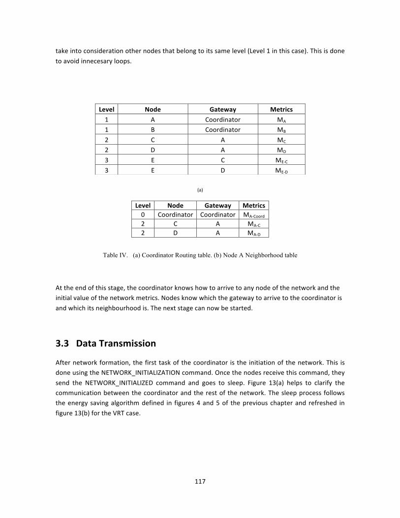
117

take into consideration other nodes that belong to its same level (Level 1 in this case). This is done to avoid innecesary loops.

(a)

Level Node Gateway Metrics 0 Coordinator Coordinator MA-‐Coord

2 C A MA-‐C

2 D A MA-‐D

Table IV. (a) Coordinator Routing table. (b) Node A Neighborhood table

At the end of this stage, the coordinator knows how to arrive to any node of the network and the initial value of the network metrics. Nodes know which the gateway to arrive to the coordinator is and which its neighbourhood is. The next stage can now be started.

3.3 Data Transmission

After network formation, the first task of the coordinator is the initiation of the network. This is done using the NETWORK_INITIALIZATION command. Once the nodes receive this command, they send the NETWORK_INITIALIZED command and goes to sleep. Figure 13(a) helps to clarify the communication between the coordinator and the rest of the network. The sleep process follows the energy saving algorithm defined in figures 4 and 5 of the previous chapter and refreshed in figure 13(b) for the VRT case.

Level Node Gateway Metrics 1 A Coordinator MA 1 B Coordinator MB

2 C A MC

2 D A MD

3 E C ME-‐C 3 E D ME-‐D

118

(a)

(b)

Fig 13. (a) Network initialization process. (b) Shows the Layer evolution for the Network Initialization

The task of the coordinator is to request the collected data to all the nodes that belong to the network. This must be done taking into account that:

(i) All the nodes are in sleep mode and only wake up for short period of time, and (ii) There will be two types of nodes:

1. Those that are in the coverage area of the coordinator 2. Those nodes that need an intermediary step (one or more than one rely node) to

communicate with the coordinator. The communication between the node and the coordinator explained in point 1 is clearly defined in figure 14.



NET_INITIALIZATION)



START_VRT))or)

START_FRT)))

VRT_STARTED))or)

FRT_STARTED)

NET_INITIALIZED)

119

Fig 14. Network data Request for those nodes that belong to the coordinator coverage area. The network packet indicates the source and destination address, the type of frame, the next hops, that in this case is the same that the destination address and the

counter node, indicating that there is only one hop

Because of the communication belongs to those nodes that are in the coordinator coverage area, only one hop is required. This is clearly identified by the counter value that is introduced in the Data section. Moreover, the receiver address and the next hop have the same value for the same reason.

The DATA_REQUEST packet is encapsulated in a FRT/VRT_REQUEST frame that is sent following the time diagram presented in figure 13(b). When the destination node starts its wake-‐up window and receives the frame, it is de-‐codified, the DATA_REQUEST packet is de-‐capsulated and a DATA_RESPONSE packet is encapsulated in a FRT/VRT_RESPONSE frame that is sent. Please observe below the format for the DATA_RESPONSE packet.

Coordinator Receiver Address

DATA_RESP 0+data length

Next hops Counter Data

This explanation helps to understand how the communication is done when some hops are necessary to reach the destination node. In multi-‐hop communications, the number of hops necessary plays an important role in reaching the destination and the addresses that will form the whole path. The algorithm is clear. The counter is correlated with the next-‐hop address. When an intermediary node is reached, the counter is decreased. The new counter value will be correlated



DATA_REQUEST)



VRT_REQUEST))or)

FRT_REQUEST)))

VRT_RESPONSE)or)

FRT_RESPONSE)

DATA_RESPONSE)

Coordinator)Receiver)Address) DATA_REQ)

Receiver)Address) 1)

)

))

)) )

)))))))))))Physical))or)Short)Address) Frame)control) ))))))Data)Section))

120

with the next hop address, which will be used for the following hop. For a better understanding of the behavior of the network communication, please see figure 15.

Fig 15. Network data Request retransmission in a three hops communication

Figure 15 shows how the communication path is defined. The stroked out address just means that this address corresponds to the previous hop, but is not removed from the packed because of it will be used for the response packet.

(a)

!

Coordinator! Node!D! DATA_REQ!

!

Node!A,!Node!C,!Node!D!

2!

! !


!


1!

!!


!


0!

!

!

Node!D! Coordinator! DATA_RESP!

!

Node!C,!Node!A,!Coord!

2! Data!

!

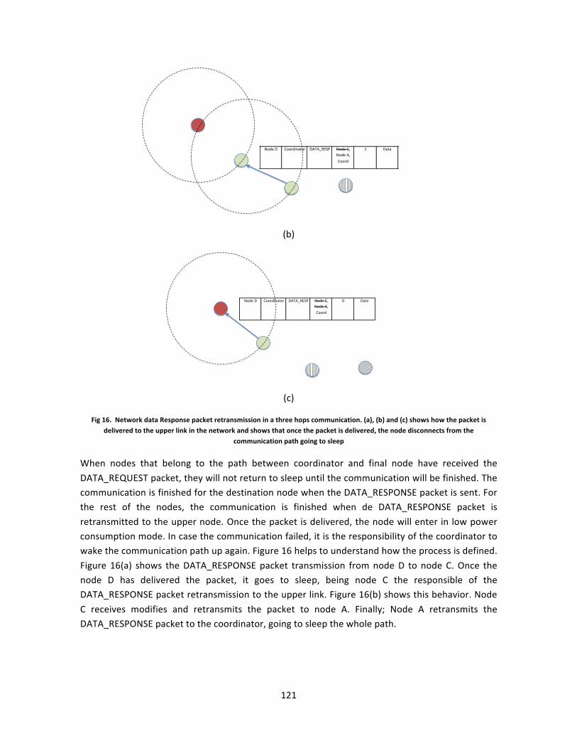
121

(b)

(c)

Fig 16. Network data Response packet retransmission in a three hops communication. (a), (b) and (c) shows how the packet is delivered to the upper link in the network and shows that once the packet is delivered, the node disconnects from the

communication path going to sleep

When nodes that belong to the path between coordinator and final node have received the DATA_REQUEST packet, they will not return to sleep until the communication will be finished. The communication is finished for the destination node when the DATA_RESPONSE packet is sent. For the rest of the nodes, the communication is finished when de DATA_RESPONSE packet is retransmitted to the upper node. Once the packet is delivered, the node will enter in low power consumption mode. In case the communication failed, it is the responsibility of the coordinator to wake the communication path up again. Figure 16 helps to understand how the process is defined. Figure 16(a) shows the DATA_RESPONSE packet transmission from node D to node C. Once the node D has delivered the packet, it goes to sleep, being node C the responsible of the DATA_RESPONSE packet retransmission to the upper link. Figure 16(b) shows this behavior. Node C receives modifies and retransmits the packet to node A. Finally; Node A retransmits the DATA_RESPONSE packet to the coordinator, going to sleep the whole path.

!


!


1! Data!

!

!


!


0! Data!

!

122

3.4 Network Management

The management of the WSN consists basically of the following statements:

• The identification of a fallen node (battery discharge, node malfunction, …) • The knowledge of the battery consumption of the network • The request from a node to transmit a data alarm

The first two statements are clearly correlated. If the network knows the battery state of the belonged nodes, the battery discharge of some of these nodes can be delayed. However, due to the need of data transmission, it is clear that nodes that belong to the network backbone core will suffer a bigger consumption and probably die before. The depletion of this backbone will lead the disconnection of some parts of the network and finally in the dead of the WSN. For this reason it is important to know which nodes need to be switched (if it is possible) and to know a priori when the network will fall.

The first point considers the possibility to transmit an alarm detected by a sheet node to the network coordinator. This will allow the alarm to respond as quickly as possible. In the following points we will describe how the network implements these different management statements.

3.4.1 Fallen node identification

In a normal data request, the DATA_REQUEST packet is transmitted through the entire path to the sheet destination node, which will respond following the same path sending a DATA_RESPONSE packet. This is the normal behavior that was explained above. However, and due to the finite live of the battery, there is a possibility that one of the nodes that belongs to the communication path will fall down during the communication process. The node-‐to-‐node communication is well known and well established at the MAC and upper LINK layers. Therefore, in cases where of any of the nodes do not respond to requests, the transmitter node will consider that something wrong is happening in that node. The following step will be the sent as a broadcast FAIL_CONNECTION packet. Figure 17 shows the state diagram and the packet structure. As can be observed, when the next hop does not respond to the request windows presented in figure 13(b), the source node sends a FAIL_CONNECTION packet, also presented in figure 17. This packet is send as a broadcast mode; because of it can no follow the path established by the coordinator. However, the value of the counter is maintained. As this counter indicates the level where the path was broken, only those nodes that are at this level or higher (higher means that they are closer to the coordinator) can retransmit this packet. Moreover, if one node at a given level has been the first to retransmit the packet; those nodes that belong to this level will NOT retransmit the packet. Finally, the FAIL_CONNECTION packet arrives to the coordinator and will be necessary to verify the node’s fault. This verification is done sending a KEEP_ALIVE_REQUEST packet from the coordinator. The different fields of this packet will be the source and destination addresses, the packet type, the number of hops and the different hop node address necessary to arrive to the destination. The response will be a KEEP_ALIVE_RESPONSE packet, and will be done either by the destination node

123

in case it is still alive or by the closest node specified by the path in case that, effectively, the node is faulty. Figure 18 shows the packet format:

Fig 17. State diagram implemented to detect if the node has fallen


KEEP_ALIVE_REQUEST Next hops Counter


KEEP_ALIVE_RESPONSE Next hops Counter TRUE or FALSE

Fig 18. Frame format for the KEEP_ALIVE request and response frames

Finally, there is the possibility that for unknown reasons, the DATA_RESPONSE packet does not reach the coordinator. In this unlikely case, the coordinator will send the KEEP_ALIVE_REQUEST, indicating in the receiver address the final address used in the previous packet. If the packet cannot continue because the node is faulty, the neighbor that detects the failure responds to the coordinator sending the corresponding KEEP_ALIVE_RESPONSE.

The$node$responds$to$the$window$request?$

Send$the$PACKET_RESPONSE$$

YES$

!

!

Node!D!

!

Coordinator!

DATA_REQ!!

or!

DATA_RESP!

Node!C,!!

Node!A,!!

Coord!

!

1!

Data!

(for!a!DATA_RESP)!

!

Send$the$FAIL_CONNECTION$

NO$

!

!

Node!D!

!

BROADCAST!

!

FAIL_DET!

!

BROADCAST!

!

1!

FAIL_NODE!

address!

!

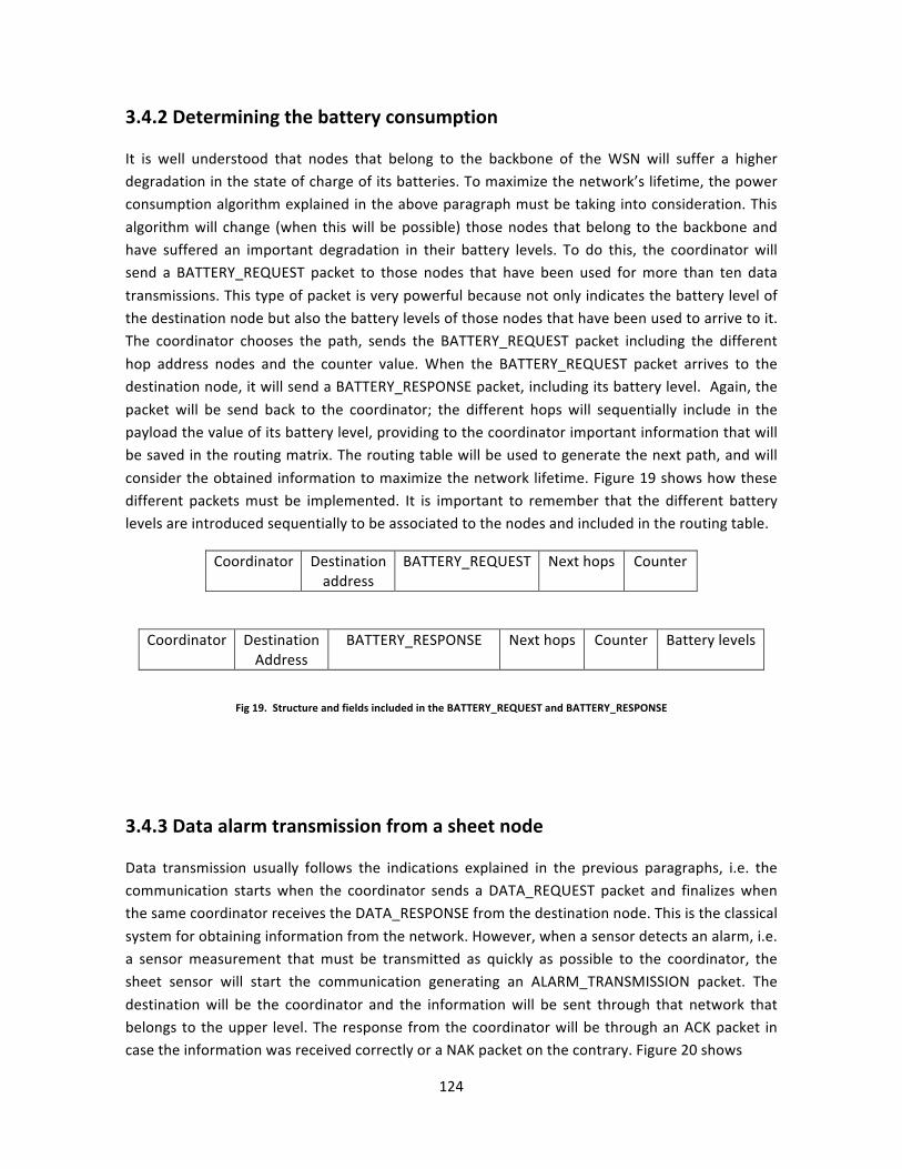
124

3.4.2 Determining the battery consumption

It is well understood that nodes that belong to the backbone of the WSN will suffer a higher degradation in the state of charge of its batteries. To maximize the network’s lifetime, the power consumption algorithm explained in the above paragraph must be taking into consideration. This algorithm will change (when this will be possible) those nodes that belong to the backbone and have suffered an important degradation in their battery levels. To do this, the coordinator will send a BATTERY_REQUEST packet to those nodes that have been used for more than ten data transmissions. This type of packet is very powerful because not only indicates the battery level of the destination node but also the battery levels of those nodes that have been used to arrive to it. The coordinator chooses the path, sends the BATTERY_REQUEST packet including the different hop address nodes and the counter value. When the BATTERY_REQUEST packet arrives to the destination node, it will send a BATTERY_RESPONSE packet, including its battery level. Again, the packet will be send back to the coordinator; the different hops will sequentially include in the payload the value of its battery level, providing to the coordinator important information that will be saved in the routing matrix. The routing table will be used to generate the next path, and will consider the obtained information to maximize the network lifetime. Figure 19 shows how these different packets must be implemented. It is important to remember that the different battery levels are introduced sequentially to be associated to the nodes and included in the routing table.

Coordinator Destination address

BATTERY_REQUEST Next hops Counter

Coordinator Destination Address

BATTERY_RESPONSE Next hops Counter Battery levels

Fig 19. Structure and fields included in the BATTERY_REQUEST and BATTERY_RESPONSE

3.4.3 Data alarm transmission from a sheet node

Data transmission usually follows the indications explained in the previous paragraphs, i.e. the communication starts when the coordinator sends a DATA_REQUEST packet and finalizes when the same coordinator receives the DATA_RESPONSE from the destination node. This is the classical system for obtaining information from the network. However, when a sensor detects an alarm, i.e. a sensor measurement that must be transmitted as quickly as possible to the coordinator, the sheet sensor will start the communication generating an ALARM_TRANSMISSION packet. The destination will be the coordinator and the information will be sent through that network that belongs to the upper level. The response from the coordinator will be through an ACK packet in case the information was received correctly or a NAK packet on the contrary. Figure 20 shows

125

Node Address

Coordinator ALARM_TRANS. Next hop Counter Relevant Information

Coordinator Destination address

ACK/NAK Next hops Counter

Fig 20. Format of each packet in communication

4. Conclusions

The main purposes of designing a routing protocol that we have investigated for wireless communications are energy efficiency, delivery latency, packet success probability, adaptability and scalability. All these parameters are used by routing algorithms to determine route optimality. Therefore, data transmission in WSN can be accomplished with discovering of neighbor nodes and later on start forwarding the packet through each other while reaching the sink or main nodes as in object. In this category packet forwarding is playing the original role of how to lead and push the packet between intermediate sensors. For that reason forwarding algorithm implements goal, for instance, the shortest average hop distance from source to destination, and also energy strategy in each sensor.

To reduce the power consumption in WSN, topology control is a good tool for extending the network lifetime, in fact topology control algorithms select the communication range of a node, and they construct and maintain a network topology based on different aspects such as node mobility, routing algorithm and energy conservation. Two topology controls such as clustering and power-‐base algorithms are explained in this study.

A routing algorithm is a way to establish correctly and efficiently the best route between each pair of nodes in the same segment of network area therefore, minimizing of energy consumption, low cost path and also minimizing overhead/delay, decreasing high bandwidth usage and increasing network lifetime are the goals of the best routing protocols in each WSN Operations.

Furthermore, we have used in our routing protocol, sections such as network formation data transmission and network management. Therefore, network formation is a way to identify all nodes and their neighbors and save them in a routing table in the coordinator node as a star network topology to decrease the activity of forwarding process to energy consumption

126

avoidance. On the other hand, data transmission is a key in organizing transmission and reception of packets for each phase of communications. In this section, each phase of packet movements would control which behaves properly, that’s why data section is a tool to help the packet control. A break-‐down of data packet and control of every transmission is main goal for achieving the best result in our routing protocol.

In addition, counter controller is a way of avoiding loops happening in WSN process. In this routing protocol with the aid of FRT and VRT, which are explained in the MAC section, try to cooperate between these two OSI layers to achieve as higher level of network optimization.

For the coordinator to manage all the communications it means all the transmissions between each node are done by the controller and only the coordinator will know where the packet should arrive. The main reason for this communication policy is just involving one node with permanent power supply to manage these activities and each node after finishing their task, may stay in sleep mode while saving energy usage when they are not in action.

In the network management section the identification of a faulty node (battery discharge, node malfunction), the knowledge of the battery consumption of the network and request from a node to transmit a data alarm was considered.

Minimizing energy consumption, finding the proper path to/from the coordinator, robustness, reliability of communication and decreasing fault errors are the main results which we concluded with this routing protocol.

127

References:

[1] I.Singh, “An Analysis of Energy Optimization algorithm in Wireless Sensor Network, " IOSR Journal of Computer Engineering (IOSR-JCE), e-ISSN: 2278-0661, p- ISSN: 2278-8727Volume 16, Issue 2, Ver. VIII (Mar-Apr.2014), PP 49-55. [2] Jamal N. Al-Karaki & Ahmed E. Kamal, “Routing Techniques in Sensor Networks: A survey”, IEEE Communications, Volume 11, No. 6, Dec. 2004, pp. 6—28. [3] Anna Hac, “Wireless Sensor Network Designs,” University of Hawaii at Manoa, Honolulu, USA, 2003. [4] F. Ye, H. Luo, J. Cheng, S. Lu, L. Zhang, “A Two-tier data dissemination model for large-scale wireless Sensor networks, “proceedings of ACM/IEEE MOBICOM, 2002. [5] J. Kulik, W. R. Heinzelman, and H. Balakrishnan, "Negotiation-based protocols for disseminating Information in wireless sensor networks," Wireless Networks, Volume: 8, pp. 169-185, 2002. [6] C. Intanagonwiwat, R. Govindan, and D. Estrin, "Directed diffusion: a scalable and robust Communication paradigm for sensor Networks," Proceedings of ACM MobiCom '00, Boston, MA, 2000, pp. 56-67. [7] D. Braginsky and D. Estrin, “Rumor Routing Algorithm for Sensor Networks," in the Proceedings of the First Workshop on Sensor Networks and Applications (WSNA), Atlanta, GA, October 2002. [8] http://nms.lcs.mit.edu/projects/leach/ [9] W. R. Heinzelman, A. Chandrakasan, and H. Balakrishnan “Energy-Efficient Communication Protocol for Wireless Microsensor Networks,” Proceedings of the 33rd Hawaii International Conference on System Sciences – 2000. [10] S. Lindsey, C. Raghavendra, "PEGASIS: Power-Efficient Gathering in Sensor Information Systems", IEEE Aerospace Conference Proceedings, 2002, Vol. 3, 9-16 pp. 1125-1130. [11] N. Rathi1, J. Saraswat, and P. P Bhattacharya, "a review on routing protocols for application in wireless sensor networks,” International Journal of Distributed and Parallel Systems (IJDPS) Vol.3, No.5, September 2012. [12] A. Manjeshwar and D. P. Agarwal, "TEEN: a routing protocol for enhanced efficiency in wireless sensor Networks," In 1st International Workshop on Parallel and Distributed Computing Issues in Wireless Networks and Mobile Computing, April 2001. [13] A. Manjeshwar and D. P. Agarwal, "APTEEN: A hybrid protocol for efficient routing and comprehensive Information retrieval in wireless sensor networks," Parallel and Distributed Processing Symposium, Proceedings International, IPDPS 2002, pp. 195-202. [14] Y. Xu, J. Heidemann, D. Estrin, “Geography-informed Energy Conservation for Ad-hoc Routing," In Proceedings of the Seventh Annual ACM/IEEE International Conference on Mobile Computing and Networking 2001, pp. 70-84. [15] Y. Yu, D. Estrin, and R. Govindan, “Geographical and Energy-Aware Routing: A Recursive Data Dissemination Protocol for Wireless Sensor Networks", UCLA Computer Science Department Technical Report, UCLA-CSD TR-01-0023, May 200. [16] B. Chen, K.Jamieson, H. Balakrishnan, R. Morris, “Span: an energy-efficient coordination algorithm for Topology maintenance in ad hoc wireless networks,” Journal Wireless Networks, Volume 8 Issue 5, Kluwer Academic Publishers Hingham, MA, USA, September 2002, pages 481-494. [17] Subramanya Bhat.M, Shwetha.D, Devaraju.J.T, “A Performance Study of Proactive, Reactive and Hybrid Routing Protocols using Qualnet Simulator,” International Journal of Computer Applications (0975 – 8887) Volume 28– No.5, August 2011. [18] T. Melodia, D. Pompili, and I. F. Akyildiz, "On the Interdependence of Distributed Topology Control and Geographical Routing in Ad Hoc and Sensor Networks," IEEE Journal of Selected Areas in Communications, vol. 23, no. 3, March 2005, pp. 520-532. [19] R.Ramanathan and R.Hain. “Topology control of multihop wireless networks using transmit power adjustment”. In IEEE INFOCOM, Tel Aviv, Israel, March 2000, pp. 404-413 [20] H. Takagi and L. Kleinrock. “Optimal transmission ranges for randomly distributed packet radio terminals,” IEEE Transactions on Communications, 32(3): 1984, pp 246—257. [21] N.ABABNEH, S. SELVADURAI “TOPOLGY CONTROL ALGORITHMS FORWIRELESS SENSOR NETWORKS: AN OVERVIEW,” International Journal on Wireless and Optical Communications, Vol. 3. No. 1, Apr. 2006, pp. 49-68. [22] L.Bao and J.J. Garcia-Luna-Aceves “Topology Management in Ad Hoc Networks,” in proceeding of the 4th ACM International Symposium on Mobile Ad Hoc Networking and Computing (MobiHoc ’03), Annapolis, MD, ACM, New York 2003, pp.40-48. [23] Y.Xu, S.Bien, Y.Mori, J. Heidemann, and D.Estrin. “Topology control protocols to conserve energy in wireless ad hoc networks,” Technical report center for embedded networked sensing technical report 6, UCLA, 2003. [24] S.Guha and S. Khuller. “Approximation algorithms for connected dominating sets, “. Algorithmica, 1998, 20(4):374-387.

128

[25] E. M. Royer and C-K. Toh, “A review of current routing protocols for ad-hoc mobile wireless networks, “IEEE Personal Communications, April 1999, pp 46–55. [26] M. I1yas, editor. The handbook of Ad Hoc Wireless Networks. CRC Press, Boca Raton, FL 2003. [27] C.E. Perkins & P. Bhagwat, “Highly Dynamic Destination-Sequenced Distance Vector Routing (DSDV) for Mobile Computers,” Proceedings of ACM SIGCOMM'94, London, UK, Sep. 1994, pp. 234-244. [28] Clausen, T., Jacquet, P.: ‘Optimized link state routing protocol (OLSR)’.IETF RFC3626, 2003, available at http//www.ietf.org/rfc/rfc3626.txt. [29] D. Johnson, Y. Hu, D. Maltz. "The Dynamic Source Routing Protocol (DSR) for Mobile Ad- hoc Networks for IPv4". RFC 4728. February, 2007. Available at https://www.ietf.org/rfc/rfc4728.txt. [30] C. E. Perkins and E. M. Royer, and S. Das. ” Ad-Hoc on Demand Distance Vector (AODV) Routing”. Request for comments 3561, February 2007. Available at http://www.ietf.org/rfc/rfc3561.txt. [31] M. J. Lee, J. Zheng, X. Hu, H. Juan, C. Zhu, Y. Liu, J. S. Yoon and T. N. Saadawi, “A new taxionomy of routing algorithms for wireless mobile ad hoc networks: The component approach”, Topics in ad hoc networks, IEEE Communications Magazine, vol.44, no. 11, pp 116, 2006. [32] Request for Comments RFC 1058, Routing Information Protocol, 1988 [33] Request for Comments RFC 2453, Routing Information Protocol version 2, 1998 [34] Request for Comments RFC 3561, Ad hoc On-Demand Distance Vector (AODV) Routing protocol, 2003 [35] A. Ephremides, “Energy concerns in wireless networks”, IEEE Wireless Communications, vol. 9, pp 48-59, 2002 [36] M. Haenggi and D. Puccinelli, “Routing in ad hoc networks: A case for long hops”, IEEE Communications Magazine, vol. 43, no. 10, pp 93, 2005 [37] J. G. Proakis, “Digital Communications”Ed. Mc Graw Hill, 4 Edition, 2001 [38] IEEE Transactions on Veh. Tech. Vol. VT-37, 1988. The Special issue on radio propagation [39] A. Ephremides “Energy concerns in wireless networks”, IEEE Wireless Communications, vol. 9, pp 48-59, 2002 [40] A. Woo, T. Tong, D. Culler, “Taming the underlying challenges of reliable multihop routing in sensor networks” Proceedings of the First International Conference on Embedded Networked Sensor Systems. Los Angeles, 2003 [41] A. J. Goldsmith and S. B. Wicker, “Design challenges for energy-constrained ad hoc wireless networks”, wireless communications, vol. 9, no. 4, pp 8-27, 2002 [42] CC2420 Datasheet, available in http://www.chipcon.com [43] R. D-Souza, D. Galvin, C. Moore and D. Randal, “Global connectivity from local geometric constraints for sensor networks with various wireless footprints”, Information Proceedings in Sensor Networks, IPSN 2006, pp 19-6. [44] R. Wattenhofer, L. Li, P. Bahl and Y. Wang. “Distributed topology control for power efficient operation in multihop wireless ad hoc networks”. In Proceedings of IEEE INFOCOM, 2001 [45] L Li, J. Y. Halpern, P. Bahl, Y. Wang and R. Wattenhofer.“Analysis of a cone=based topology control algorithm for wireless multihop networks”. Proceedings of ACM symposium on Principles of Distributed Computing, 2001 [46] K. Benkič, M. Malajner, P. Planinšič, Ž. Čučej. “Using RSSI value for distance estimation in Wireless sensor networks based on ZigBee” SPaRC Laboratory, UM-FERI Maribor, Smetanova 17, Maribor, 2000, Slovenia

129

Chapter 5. Experimental Results

130

1 The simulation tool

In the last years, the study of design, development and implementation of WSN is a hot research topic. Many network details in WSNs are still not finalized and standardized. Building a WSN test-‐bed is very costly because of needing to implement a huge quantity of wireless sensor nodes and a large area is needed to implement it. Besides, repeatability is largely compromised since many factors affect the experimental results at the same time. It is hard to isolate a single aspect. Moreover, running real experiments are always time consuming. Therefore, WSNs simulation is important for WSNs development. Protocols, schemes, even new ideas can be evaluated in a very large scale. WSNs simulators allow users to isolate different factors by tuning configurable parameters.

Consequently, simulation is essential for studying WSNs, being the common way to test new applications and protocols in the field. This leads to the recent boom of simulator development.

However, obtaining solid conclusions from a simulation study is not a trivial task. There are two key aspects in WSNs simulators: (1) The correctness of the simulation models and (2) the suitability of a particular tool to implement the model. A “correct” model based on solid assumption is mandatory to derive trustful results. The fundamental tradeoff is: precision and necessity of details versus performance and scalability.

1.1 Summary of simulators for WSN

This section shows different main-‐stream simulation tools used in WSN. Some of them have been analyzed and studied in several research papers. Others are used as a simulation tool for engineering companies. We will try to analyze the advantages and disadvantages of each of them.

1.1.1 NS-‐2

NS-‐2 is the abbreviation of Network simulator version two, developed at the end of the 80’s for the first time. This simulator is used as the real network simulator. Nowadays, the NS-‐2 is supported by the Defense Advanced Research Projects Agency and the National Science Foundation. The NS-‐2 is a discrete event network simulator built in object oriented extension of tool command language and C++. This software runs on Linux Operating systems or using Cygwin over Windows.

NS-‐2 can support a considerable range of protocols in all layers. For example, the ad-‐hoc and WSN specific protocols are provided by NS-‐2. The open source model saves the cost of simulation, and online documents allow the users easily to modify and improve codes.

131

However, this simulator has some limitations. Firstly, people who want to use this simulator need to be familiar with writing scripting language and modelling techniques; the Tool Command Language is somewhat difficult to understand and write. Secondly, sometimes using NS-‐2 is more complex and time-‐consuming than other simulators to model a desired job. Thirdly, NS-‐2 provides a poor graphical support, there is no Graphical User Interface (GUI); the users have to directly face text commands of the electronic devices. Fourthly, due to the continuing changing of the code base, the result may not be consistent, or contains bugs. In addition, since NS-‐2 is originally targeted for IP networks but not WSNs, there are some limitations when simulating WSNs. Firstly, NS-‐2 can simulate the layered protocols but not application behaviours. However, the layered protocols and applications interact and cannot be strictly separated in WSNs. Therefore, in this situation, using NS-‐2 is inappropriate, and it can be hard to acquire correct results. Secondly, because NS-‐2 is designed as a general network simulator, it does not consider some unique characteristics of WSN. For example, NS-‐2 cannot simulate bandwidth problems, power consumption or energy saving in WSN. Thirdly, NS-‐2 has a scalability problem in WSN, it has trouble simulating more than 100 nodes. As the number of nodes increases, the tracing files will be too large to management. Finally, it is difficult to add new protocols or node components due to the inherent design of NS-‐2. To sum up, NS-‐2 as a simulator of WSN contains both advantages and disadvantages.

1.1.2 TOSSIM

TOSSIM [1, 2, 3, 4, 5, 6, 7, 8] is an emulator specifically designed for WSN running on TinyOS, which is an open source operating system targeting embedded operating system. In 2003, TOSSIM was first developed by UC Berkeley’s TinyOS project team. TOSSIM is a bit-‐level discrete event network emulator built in Python[9], a high-‐level programming language emphasizing code readability, and C++. People can run TOSSIM on Linux Operating Systems or on Cygwin on Windows. TOSSIM also provides open sources and online documents.

TOSSIM contains both merits and limitations when used to emulate WSNs. For the merits, the open source model free online document to save the emulation cost. Also, TOSSIM has a GUI, TinyViz, which is very convenient for the user to interact with electronic devices because it provides images instead of text commands.

In addition, TOSSIM is a very simple but powerful emulator for WSN. Each node can be evaluated under perfect transmission conditions, and using this emulator can capture the hidden terminal problems. As a specific network emulator, TOSSIM can support thousands of nodes simulation. This is a very good feature, because it can simulate the real world situation more accurately. Besides networks, TOSSIM can emulate radio models and code executions. This emulator may provided more precise simulation results at component levels because of compiling directly to native codes.

However, this emulator still has some limitations. Firstly, TOSSIM is designed to simulate behaviours and applications of TinyOS, and it is not designed to simulate the performance metrics

132

of other new protocols. Therefore, TOSSIM cannot correctly simulate issues of the energy consumption in WSN; people can use PowerTOSSIM [10], another TinyOS simulator extending the power model to TOSSIM, to estimate the power consumption of each node. Secondly, every node has to run on NesC code, a programming language that is event-‐driven, component-‐based and implemented in TinyOS, thus TOSSIM can only emulate the type of homogeneous applications. Thirdly, because TOSSIM is specifically designed for WSN simulation, motes-‐like nodes are the only thing that TOSSIM can simulate. To sum up, TOSSIM as an emulator of WSN contains both advantages and disadvantages.

1.1.3 OMNeT

OMNeT++ is a discrete event network simulator built in C++. OMNeT++ provides both a non-‐commercial license, used at academic institutions or non-‐profit research organizations, and a commercial license, used at "for-‐profit" environments. This simulator supports module programming model. Users can run OMNeT++ simulator on Linux Operating Systems, Unix-‐like system and Windows. OMNeT++ is a popular non-‐specific network simulator, which can be used in both wire and wireless area. Most of the frameworks and simulation models in OMNeT++ are open sources.

OMNeT++ contains both merits and limitations when used to simulate WSNs. To the merits, firstly, OMNeT++ provides a powerful GUI. This strong GUI makes the tracing and debugging much easier than using other simulators. Although initial OMNeT++ do not support the module library which is specifically used for WSNs simulation, with the consciously contribution of the supporting team, now OMNeT++ has a mobility framework. This simulator can support MAC protocols as well as some localized protocols in WSN. People can use OMNeT++ to simulate channel controls in WSNs. In addition, OMNeT++ can simulate power consumption problems in WSNs. However, there are still some limitations on OMNeT++ simulator. For example, the number of available protocols is not larger enough. In addition, the compatibility problem will rise since individual researching groups developed the models separately, this makes the combination of models difficult and programs may have high probability report bugs. To sum up, both advantages and disadvantages are included in the OMNeT++ design [4, 12, 13].

1.1.4 OPNET

OPNET Technologies is a software business that provides performance management for computer networks and applications [17]. It is commercial software similar to OMNeT and specially designed and optimized for wired networks. It does not consider WSN as a standard communication protocols and the installation of complicated plugins to work with these kind of networks are needed.

133

1.1.5 J-‐Sim

J-‐Sim is a discrete event network simulator built in Java. This simulator provides GUI library, which facilities users to model or compile the Mathematical Modelling Language, a “text-‐based language” written to J-‐Sim models. J-‐Sim provides open source models and online documents. This simulator is commonly used in physiology and biomedicine areas, but it also can be used in WSN simulation. In addition, J-‐Sim can simulate real-‐time processes.

J-‐Sim has both merits and limitations when used to simulate WSNs. For the merits, firstly, models in J-‐Sim have good reusability and interchange ability, which allows for easy simulation. Secondly, J-‐Sim contains a large number of protocols; this simulator can also support data diffusions, routings and localization simulations in WSNs by detail models in the protocols of J-‐Sim. J-‐Sim can simulate radio channels and power consumptions in WSNs. Thirdly, J-‐Sim provides a GUI library, which can help users to trace and debug programs. The independent platform is easy for users to choose specific components to solve the individual problem. Fourth, comparing with NS-‐2, J-‐Sim can simulate a larger number of sensor nodes, around 500, and J-‐Sim can save lots of memory sizes. However, this simulator has some limitations. The execution time is much longer than that of NS-‐2. Because J-‐Sim was not originally designed to simulate WSNs, the inherent design of J-‐Sim makes users unable to add new protocols or node components [4, 5, 13, 14 ].

1.1.6 EmStar

EmStar [15, 16] is an emulator specifically designed for WSN built in C, and it was first developed by University of California, Los Angeles. EmStar is a trace-‐driven emulator running in real-‐time. This emulator can be run on Linux operating system. This emulator supports to develop WSN application on better hardware sensors. Besides libraries, tools and services, an extension of Linux microkernel is included in EmStar emulator.

EmStar contains both merits and limitations when to simulate WSNs. For the merits, firstly, the modular programming model in EmStar allows the users to run each module separately without sacrificing the reusability of the software. EmStar has a robustness feature that can mitigate faults among the sensors, and it provides many modes making debugging and evaluating much easier. There is a flexible environment in EmStar that users can freely change between deployment and simulation among sensors. Also with a standard interfaces, each service can easily be interconnected. EmStar has a GUI, which is very helpful for users to control electronic devices. When using EmStar, every execution platform is written by the same codes, which will decrease bugs when the separate modes iterate. In addition, EmStar provides many online documents to facilitate the wide use of this emulator. However, this emulator contains some drawbacks. For example, it cannot support large numbers of sensors simulations, and the limited scalability will decrease the reality of simulation, shown in Figure 5. In addition, EmStar can only run in real time simulation. Moreover, this emulator can only apply to iPAQ-‐class sensor nodes and MICA2 motes. All these drawbacks limit the use of this emulator. To sum up, both advantages and disadvantages are included in the EmStar design.

134

Due to the difficulty in finding a simulator that permits us to adjust and simulate the behaviour of the sensor nodes as a function of the power consumption, channel selection and other important characteristics of the physical layer we have decided to design our own simulator. This simulator was developed in Python. It includes libraries as numpy, for numerical operations, arrays and matrix development, matplotlib for plotting the different graphs, and other specific libraries [1, 3, 4, 7, 15, 16].

1.2 The developed simulator: WSN_PySim

WSN_PySim is a WSN specifically designed to study the lifetime of the network, taking into account the channel behaviour, the Signal-‐to-‐Noise Ratio (SNR), the interferences and the Packet Error Rate (PER).

Python is a high level, general purpose, interpreter, object oriented programming (OOP) language that provides a large quantity of libraries and on-‐line help the eases the development of the program. The integrated development environment used for programming the simulator was Spyder, an open source cross-‐platform for scientific programming in Python language. Spyder integrates NumPy, SciPy, Matplotlib and Python, as well as other open source software.

Spyder includes support for interactive tools for data inspection and embeds Python specific code quality assurance and introspection instruments. In our particular case, we found it embedded in the Anaconda cross-‐platform. As a well IDE, Spyder permits the debugging of the code and the execution line by line, the possibility to analyse and modify the values of variables and continue executing the code with these new values.

Figure 1 represents the code structure of the simulator. The main function, implemented in the main class calls to the Physical Layer class, the MAC Layer class, the Routing Class and finally Application Class.

135

Fig 1. Block diagram that shows the structure of the simulator’s code. This figure also shows the main goals of every block.

1.2.1 Main class

The main function is the user interface, request the number of nodes, the area for the node distribution and finally perform a Gaussian random distribution. Once the distribution is generated the simulation begins calling in the other classes. Figure 2 shows an example of 20 nodes randomly distributed in an area of 800 m2. The mean value in this case is centred to 0 and the standard deviation is 20 m for both axes.

MAIN%

PHYSICAL%LAYER%CLASS%

MAC%%LAYER%CLASS%

NETWORK%LAYER%CLASS%

APPLICATION%LAYER%CLASS%

2%Random%node%distribu?on%2%Call%to%the%other%classes%2%Representa?on%of%the%network%%%life?me%

2  SNR%calcula?on%2  Channel%effect%2  PER%calcula?on%2  Rx%Power%

2  MAC%layer%format%

2  Duty%Cycle%?me%sublayer%for%power%consump?on%%

2  Metrics%genera?on%

2  Best%path%matrix%es?ma?on%

2  Rou?ng%path%vector%generated%

2  Determina?on%of%the%WSN%life?me%

136

Fig 2. Gaussian random distribution of 20 nodes in a 800 m2 square area.

The program will also ask for the coordinator, coordinates and fit the best result among the different distributed nodes. Figure 3 shows this part of the program that permits selecting where the coordinator is located in the WSN area and also calculates the relative distance between the coordinator and every node of the network. Note that the third value is 0. It is because this is the coordinator index.

Fig 3. Capture image that shows the request of the coordinator index. The program calculates provides the real values and the

distance from the coordinator to the rest of the nodes.

indica&la&coordenada&x&del&node&coordinador&>&0&indica&la&coordenada&y&del&node&coordinador&>&0&els&index&del&coordinador&trobats&son&>&&2&2&les&coordenades&del&coordinador&son&>&&5.89760859545&:2.03634981895&&Distancia&rela>va&al&coordinador&de&la&resta&de&nodes:&&[10.709417172548472,&27.770709213221352,&0,&30.320300851734707,&12.748122182744751,&52.369245624087597,&4.8884405553922265,&34.220483301274719,&19.118679571630594,&33.833761507494962,&7.2172779032776448,&10.133734234696901,&45.831128341814299,&21.244511458997106,&49.02201512370587,&56.708227797265458,&30.802214428332,&18.194060705571157,&18.62746219041091,&16.750091998423152]&

137

1.2.2 Physical Layer

The physical layer is responsible for and must provide the main class with the channel effect, the SNR and the PER calculation. The physical layer must take into account that IEEE 802.15.4 codifies the data in O-‐QPSK. To do this, the physical layer generates a random bit distribution and codifies it following the standard. Considering the selected channel that can be Rayleigh, Rice or log normal, a random white noise distribution, the possible interference effects and the distance the simulator calculates the SNR and the PER. Figure 4 shows different possibilities depending on the distance and the channel selected. For this particular case, the channel selected is a Rayleigh channel. The different nodes are located at 15 m, 20 m, 30 m and 50 m from the coordinator.

Fig 4. Estimation of the SNR and BER for a Gaussian distributed network under a Rayleigh channel. The different signals were

calculated for 15, 20, 30 and 50 m from the coordinator.

138

1.2.3 Link Layer

The link layer is responsible for the point-‐to-‐point communication. It is responsible for generating the MAC frame and introducing the power consumption associated with the duty cycle sub-‐layer. This part is one of the most important goals of this thesis because depending on the duty cycle the lifetime of the network will increase more or less. An initial value of 7500 mWatts-‐hour is assigned to every node. The coordinator is connected to the mains. Depending on the duty cycle, the power consumption will be longer or shorter. In this sense, for a duty cycle of 10% and a star configuration, the network will have a lifetime of 30 days approximately. In chapter three we indicated how the duty cycle sub-‐layer is implemented in real networks. However, in a simulation it is not exactly the same. The protocol clearly defines the time spend in the period indicated in Figure 5a: 60 seconds. Then depending on the number of nodes we know the energy spent in this period.

(a)

(b)

Fig 5. (a) Initial frame sent by the coordinator to those nodes that can bellow to the network. (b) Initiation of the VRT Energy saving algorithm

The energy spent in the starting VRT period is negligible compared with the rest of the process. Once the duty cycle sub-‐layer is initiated, the consumption is 60mWatts when the nodes are active and 60 uWatts when the nodes are in sleep mode (Figure 6).


Broadcast)Node)Request)

Node_Response)(Unicast))


START_VRT)(broadcast)mode))

VRT_STARTED)(Unicast))

139

Fig 6. Evolution of the power consumption as a function of the time.

1.2.4 Network Layer

This class defines the best path from the coordinator to every node of the network. To do this, a global matrix is calculated with all the possible neighbours and their associated PER. Depending on the accepted PER level, some routes will be permitted and some of them will be removed. The metrics used to construct this matrix was well defined in chapter 4. This global matrix was technically defined as a python dictionary, where the key was the node and the value was a list with the neighbours and the associated PER.

When a destination node is defined and transmitted to the network layer, the coordinator selects the best route to minimize the power consumption of the whole network, maximize the success probability and also minimize (if it is possible) the number of hops.

When the coordinator is not able to reach any destination node we will consider that the network has died and we will stop the simulation.

To implement this part of the program, the network layer will receive the notification of dead nodes from the main function and will introduce the necessary modification in the global matrix and the routing path. When a requested path required by the main function is not possible to achieve, the network layer notifies the death of the network and then, the main function ends the simulation.

1.2.5 Application Layer

The application layer class defines the destination node, just implementing a random selector function that takes into account to discard dead nodes and the coordinator. The application node is also responsible for decreasing the energy spent in the route formation and notifying the network layer through the main when a node has died.

Time%(mseconds)%

Power%(m

Wa2

s)%

3  60%mWa2s%

3  60%uWa2s%

Ac8ve%period%

140

2 The experimental devices

Two experimental devices were used in this thesis:

-‐ The network Coordinator, based on the Texas Instruments CC3200 microcontroller -‐ The sensor nodes, which can act as a final device or router depending on its position.

The sensor nodes used in this thesis are based on the well-‐known Tmote Sky. Figure 12 shows the block diagram of the node. The electronic system can be directly connected to a PC or laptop thru an USB connection. On the contrary to the Tmote Sky, this connection is just to transmit specific data to the PC, not for programming purposes. The programming of this board is done by a 4-‐vias JTAG connector. More information about these nodes can be obtained in chapter 2. Figure 7(a) reproduces the sensor node’s block diagram that was also explained in chapter 2. Figure 7(b) shows an image of one of these nodes.

(a)

(b)

Fig 7(a). Block diagram of the real sensor node. (b) Final design of the sensor node. On the left we show the BOTTON layer. On the right we have the TOP layer

The coordinator node is based on the Texas Instruments CC3200 Launchpad and evaluation development platform for the CC3200 wireless microcontroller. A programmable device with built-‐

FT232RQ'USB'MSP430F1611'

CC2520' CC2591'

SMA'5'SMD'

POWER'SUPPLY' CONN'1' CONN'2'

CONN'3' CONN'4'

Flash'

JTAG'

141

in WiFi connectivity, board features on-‐board emulation using FTDI and includes some sensors. This board can be directly connected to a PC for use with development tools.

Figure 8 shows a capture of this Launchpad. We have circled the two connectors that allow access to the GPIO and some specific pines of the CC3200. These connectors were used to adapt a specifically designed board, necessary to connect both the CC3200 Launchpad and CC2520 daughter board. More information about the coordinator node can be found in chapter 2.

The coordinator acts as a gateway, connecting the WSN to the Internet thru any WiFi connection and to the IEEE 802.15.4 based WSN thru the CC2520 evaluation kit, i.e., the prototype acts as a gateway between the WSN and the Internet.

Fig 8. Coordinator of the WSN based on the CC3200 Launchpad plus the CC2520 development kit. A necessary adaptation board is necessary to connect both modules. The Gerber file is also shown.

142

3 Power Consumption and lifetime Analysis

Power consumption is the main concern in developing Wireless Sensor Network applications. Among the different strategies to minimize the energy consumed, in this thesis we have chosen to implement a duty cycle in the link layer that permits to switch on and off the wireless transceiver and pass the state of the microcontroller to those that minimizes its energy. These strategies help to predict the WSN lifetime. Furthermore, due to the inherent dynamism of WSNs, the instrumentation required for measurement techniques, the necessary number of nodes to implement and the broad area needed to distribute the network, for evaluating the power consumption of WSN requires the use of simulators to predict the lifetime of WSN applications. In order to evaluate the proposed approach, it is necessary to compare the experimental results with the simulation studies.

3.1 The star configuration

When the distance between the coordinator and the rest of nodes that belong to the WSN permits a direct link, without the need of router devices, we have a star configuration. In this case, the lifetime will depend on the link’s PER. The first simulation that we have done consisted of a simple network with 5 nodes: One coordinator and four end devices. Table I shows the distances between nodes and coordinator, the reception power, the BER and finally, the lifetime of every node. Figure 9 shows the node distribution for this network. The selected duty cycle for this simulation was 1%.

Fig 9. WSN composed by 5 nodes. The node distribution was randomly obtained.

Node Distance (m)

Reception Power (dBm)

BER Lifetime (days)

#1 3.84 -‐64 0 662.64 #2 8.45 -‐71.6 0 662.64 #3 8.56 -‐71.8 0 662.64 #4 6.7 -‐69.8 0 662.64

Table I. Parameters obtained from a star configuration obtained by the simulator.

143

From the results obtained in this simulation, we obtain that, independently of the number of nodes, if the configuration of the WSN is a star configuration; the distance is short enough for obtaining a minimum BER, then the lifetime is the longest possible, depending on the duty cycle chosen. In this sense, the minimum duty cycle for a period of 1 second would be tRX window ≥ 2 ·∙ SyncHeader+length+MACframe + inter frame spacing, which means in terms of time: 32 μsec ·∙ [2 ·∙ 5 + 1 + MACframe] + inter-‐frame-‐spacing. When the permitted PER is higher than zero, the tRX window must consider the error probability and be wider in order to correctly receive the frame from/to the coordinator.

As seen in the previous equations, the inter-‐framespacing should be as short as possible, within the limits specified by the standard, to reduce power consumption. The IEEE 802.15.4 standard specifies two parameters for the minimum allowed time within consecutive frames: LIFS (Long Inter-‐Frame-‐Spacing) is 40 symbols (640 μs) long and applies to MAC frames longer than 18 bytes, and otherwise SIFS (Short Inter-‐Frame-‐Spacing) that is 12 symbols (192 μs) long. Then, the minimum tRX window = 608 μsec for a period time of 1 sec.

Five nodes were manually distributed at a constant distance from the coordinator of 20 m. The duty cycle was configured to 10%. Table II shows the reception power, the distance, the packet error rate and the lifetime.

Node Distance (m)

Reception Power (dBm)

BER (%)

Lifetime (days)

#1 20 -‐72.3 0.0012 61 #2 20 -‐71.6 0.0008 62 #3 20 -‐72.8 0.0014 61 #4 20 -‐70.8 0.0009 62 #5 20 -‐71.5 0.0013 61

Table II. Parameters obtained from a star configuration and collected by the coordinator.

From Table II column 3 (BER) we observe a non zero probability of error. In fact, a BER of 0.0012 corresponds to a PER that will depend on the size of the frame. In this sense, for a mean frame size of 20 Bytes, We obtain a PER of 82.52%.

On the other hand, if we compare the lifetime obtained at table II with those obtained in table I, we observe that, between the results obtained by the simulator and the experimentally measured, there is a linear dependence that does not depend on the PER. For a duty cycle of 1%, the lifetime of the nodes is about 600 days. For a duty cycle of 10% the lifetime is of about 60 days. Why is there no dependence on the PER? The reason is the duty cycle that we have in the real case. A 10% of duty cycle means that nodes have their transceiver wake up and fully operative for 100 msec. This time is enough to retransmit the frames not received without practically any additional operative time.

144

The selection of this duty cycle was basically a viability reason. The network was working at the lab for two months and the coordinator was sending the collected data to the database. A decrease of 1% of the duty cycle will imply a dependence of lifetime with the retransmission process associated to the PER.

Simulation was also done with the same distribution as the real network. Figure 10 shows the node distribution. At the center, the coordinator is placed. The distance between the coordinator and the rest of the nodes is 20 m, the duty cycle was 10%. The lifetime obtained for all the nodes was equal to 66.26 days and the BER obtained was 0 for all the nodes.

Fig 10. Node distribution for a star network with the coordinator.( centered at the middle of the network)

The reception power is -‐65.2457 dBm and is also identical for all the nodes. Figure 11 shows the evaluation of the BER for four of the different nodes that belong to the network. It is clear that the real world introduced effects that weren’t taken into account in the simulator; however, the comparison between simulation and real world is accepted as a first approximation of the problem and will help us to understand the behavior of our network.

145

Fig 11. SNR and BER calculation estimated by the simulator.

146

3.2 Tree Configuration

This is the most typical WSN configuration, where more or less dense deployed static sensor nodes are distributed around a static sink or coordinator. Because sensed data is collected at the sink, sensors closer to the coordinator consume more energy and have a shorter lifetime. The lifetime of the WSN will depend on the possibility of the deployed nodes to send data to the sink. The research for the best path to connect any node with the sink depends on the chosen metrics and the involved algorithm. In previous chapters we have developed the algorithm based on the duty cycle of the network and what we obtain is a hybrid protocol that mesh the network and routing layer with the link layer. It is possible to find literature in a lot of papers that talk extensively about routing algorithms for minimizing the power consumption, but, if the transceiver continues ON, and there is no integration between LINK and routing layers, the network will die in a few days.

3.2.1 First exercise: Simulation of a tree WSN

The simulation consist on a coordinator and 8 nodes randomly distributed with a standard deviation of 30 m. Table III shows the distance among the different nodes and the coordinator, the reception power and the BER. The duty cycles is again 10%

NODE PRX (dBm) Distance (m) PER (Coord-‐to-‐node)

Hop-‐to-‐Coord

#1 -‐75.6 46 0.015 Direct #2 -‐73.41 31 0.003 Direct #3 -‐76.5 53 0.297 1 #4 -‐75.5 45 0.11 2 #5 -‐75.2 43 0.225 1 #6 -‐74.3 37 0.061 2 #7 -‐77.5 62 0.365 2 #8 -‐80.3 63 0.382 1

Table III. Main characteristics of a Gaussian random distributed WSN with 30m standard deviation.

The lifetime of the network was 18 days and 10 hours approximately. The first node with battery exhausted was node 1. When it happened, half of the WSN was unconnected. Node 2 was the next in fall down taking 10 hours more than the first one in die. Because of this kind of network is a centralized one, the routing table and the path is determined by the coordinator. It means that the router nodes (1 and 2) didn’t have implemented any routing table. They just work as an access point, re-‐sending the frame to the node specified by the coordinator following the algorithm explained in chapter 4. The coordinator has all the possible combinations (stored as a list of list). For this particular case, it would be interesting try to access to nodes #3, #5 and #8 once node #1 was exhausted. Node #2 had the possibility to access to node #5 but no connection was possible with nodes #3 and #8. These nodes remained isolated and from the point of view of the coordinator these nodes were out of the WSN.

147

Figure 12 shows the node distribution. The circumferences illustrate the influence area of the different nodes and provide a global vision of the network. Figure 12 also shows the existing distance between intermediate nodes (#1 and #2) with those nodes that depend on for transmitting its collected data to the coordinator. One characteristic of the simulator is the possibility of associating some interference objects that increase the error probability. This is the case for nodes #5 and #6. For this reason it is better (from the point of view of reliability and bit error minimization) to add an additional hop between them and the coordinator.

Fig 12. WSN based on a central coordinator and 8 peripheral nodes. Nodes #1 and #2 act as a passive routers or access points to improve the communication of the network. Circumferences mean the influence area associated to that node located on its center.

As a conclusion of this simulation, we observe that the lifetime of this network is low. This is because of the high distances between nodes that introduce moderates PERs. Another reason for the low lifetime is the duty cycle. As we previously analyzed, a duty cycle of 10% for a star configuration provided a lifetime of 60 days approximately. A minimization of the duty cycle and the inclusion of intermediate nodes to decrease the PER would increase the lifetime.

The introduction of nodes like those presented in figure 13 introduces a new behavior in the WSN. The increase of density close to the coordinator can be adjusted to a different distribution that those presented in figure 12. In figure 12, the node distribution follows a Gaussian distribution, centered in the coordinator and with a standard deviation of 20 m. The distributions presented in figure 13 follows the classical Poisson distribution with a higher concentration near the coordinator and node depletion when the distance increases. This distribution, however, permits the introduction of load balancing in the communication process, distributing the power consumption between the surround nodes.

!!!"

46m"

31"m" !!!"

!!!"

#2"

#1"

#3"

#8"

#5"

Interference"object"

#4"

#6"

#7"

#4""""20m""""!50"dBm""""0"#6""""12m""""!43"dBm""""0"#7""""30"m"""!62"dBm""""0"

#3""""10m""""!40"dBm""""0"#5""""20m""""!51"dBm""""0"#8""""32m""""!64"dBm""""0"

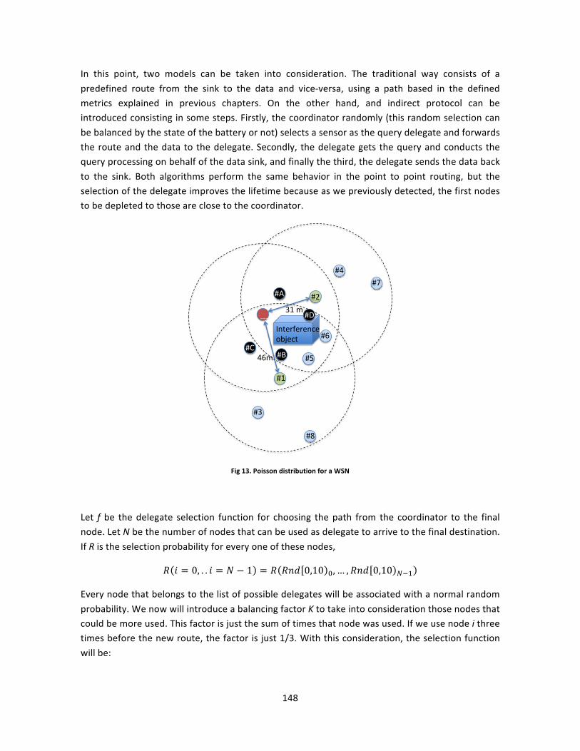
148

In this point, two models can be taken into consideration. The traditional way consists of a predefined route from the sink to the data and vice-‐versa, using a path based in the defined metrics explained in previous chapters. On the other hand, and indirect protocol can be introduced consisting in some steps. Firstly, the coordinator randomly (this random selection can be balanced by the state of the battery or not) selects a sensor as the query delegate and forwards the route and the data to the delegate. Secondly, the delegate gets the query and conducts the query processing on behalf of the data sink, and finally the third, the delegate sends the data back to the sink. Both algorithms perform the same behavior in the point to point routing, but the selection of the delegate improves the lifetime because as we previously detected, the first nodes to be depleted to those are close to the coordinator.

Fig 13. Poisson distribution for a WSN

Let f be the delegate selection function for choosing the path from the coordinator to the final node. Let N be the number of nodes that can be used as delegate to arrive to the final destination. If R is the selection probability for every one of these nodes,

𝑅 𝑖 = 0, . . 𝑖 = 𝑁 − 1 = 𝑅 𝑅𝑛𝑑 0,10 !,… ,𝑅𝑛𝑑 0,10 !!!

Every node that belongs to the list of possible delegates will be associated with a normal random probability. We now will introduce a balancing factor K to take into consideration those nodes that could be more used. This factor is just the sum of times that node was used. If we use node i three times before the new route, the factor is just 1/3. With this consideration, the selection function will be:

!!!"

46m"

31"m"!!!"

!!!"

#2"

#1"

#3"

#8"

#5"

Interference"object"

#4"

#6"

#7"#A"

#B"#C"

#D"

149

𝑓(𝑖 = 0,… 𝑖 = 𝑁 − 1) = 𝑀𝐴𝑋(1𝐾!×𝑅!)

The different paths, for the example have shown in figures 13 and 14. The need of perform a load balance is clear to maximize the lifetime of the network and improve its behavior. The options presented in this figure shown the different routes that can be established from the first disc or coordinator neighborhood with the rest of the network. Connections between disc nodes are not considered to avoid the possibility of infinite loops.

Fig 14. Possible routes from the first disc section to the rest of network

Table IV shows the attenuation and the PER for the coordinator neighborhood. These values and the routing matrix are independent of the selected algorithm (Traditional or Indirect).

NODES #1 #2 #A #B #C #D Distance to coordinator (m) 46 31 20 27 25 28 Reception Power (dBm) -‐75.6 -‐73.41 -‐66 -‐68.6 -‐67.9 -‐68.9 PER (%) 0.015 0.003 0 0.0015 0 0.002 Direct links #3,#5,#8 #6,#7,#4 #4,#6 #3,#5 #3,#5 #6,#7,#4

Table IV. Main characteristics of the coordinator’s neighbor nodes

When the network implements the traditional algorithm, there is a sequential exhausting of the nodes. This is because there is no load balance algorithm implemented. In the worst case, the first

#2#

#1#

#3#

#8#

#5#

#4#

#6#

#7##A#

#B##C#

#D#

150

two exhausted nodes are #A and #C, that take about 712h. From the simulation we observe that next exhausted node is #D, followed by #1, #B and #2. The results were iterated to obtain a mean lifetime, the value of which is presented in figure 15.

On the contrary, the results presented in figure 16a shows the behavior of the network taking into account the indirect algorithm presented above. These results have been obtained by means of a Montercarlo simulation with 10 independent iterations. Dark square indicates the lowest lifetime for this scenario. The error bar indicates the different changes obtained during the simulation. Depending on the random value generated, the first exhausted nodes can change.

500 750 1000 1250 1500

6

7

8

9

10

11

12

Aliv

e no

des

time (hours )

Fig 15. Time evolution for the alive nodes in the WSN.( previously described following the traditional algorithm)

Figure 16a shows the lifetime evolution as a function of the selection probability. The square limit shows the worst case limit, the vertical line represents the limit for the best case limit. The first thing that we want to highlight is the deep decay of the network. If we compare both methods, the associated to the traditional algorithm presents a soft decay, starting at 750 hours approximately. In case of battery replacement, it is better a sharp decay in order to exchange all the batteries at the same time.

Moreover, if we compare the plateau of both evolutions, it is clear that the indirect algorithm provides all the nodes alive for longer times. This parameter is important because of an increase of the exhausted nodes introduce a loose of performance on the whole network. Figure 16b shows a comparative of both algorithms. Please note the sharp decrease in the lifetime for the indirect algorithm and the smoother evolution for the traditional one.

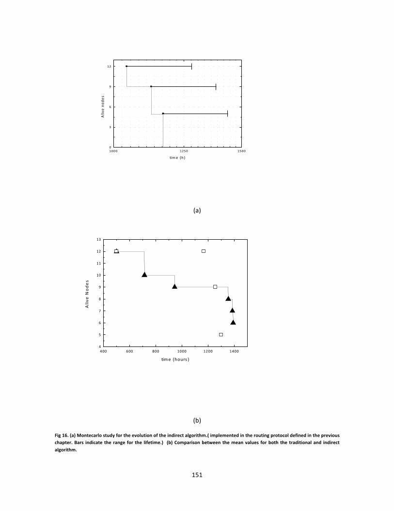
151

1000 1250 15000

3

6

9

12

Aliv

e no

des

time (h)

(a)

400 600 800 1000 1200 14004

5

6

7

8

9

10

11

12

13

Aliv

e Nod

es

time (hours )

(b)

Fig 16. (a) Montecarlo study for the evolution of the indirect algorithm.( implemented in the routing protocol defined in the previous chapter. Bars indicate the range for the lifetime.) (b) Comparison between the mean values for both the traditional and indirect algorithm.

152

4. Comparison with other algorithms

The first protocol implemented for the comparison is Ad-‐hoc On-‐demand Distance Vector (AODV) [18]. AODV is a routing protocol developed in 2003 in Nokia Research Center initially developed for using in Mobile Ad-‐hoc Networks (MANETs), but does not depend on any particular physical layer and works even in wired networks. AODV is a reactive algorithm, i.e. Routes are established on-‐demand, as they are needed. However, once established, a route is maintained as long as it is needed. Reactive (or on-‐demand) routing protocols find a path between the source and the destination only when the path is needed. The algorithm guarantees loop-‐free routes even when repairing links and scales to large networks since it does not rely on periodic advertisements. AODV defines several messages that are used during the broadcast route discovery procedure.

The metric that Perkins and Royer, presented in their article minimizes the number of hops, and therefore the latency among communication pairs. AODV implicitly balances the load of the network due to the collision avoidance mechanisms used in the MAC layer. That part of the communication stack ensures that not all nodes could transmit the Route Request (RREQ) packages at the same time. The first discovered route, with minimum number of hops is communicated to the involved nodes and used until the link is broken or explicitly a new route discovery procedure starts.

The Zigbee routing algorithm is another candidate for comparison. The ZigBee Alliance [19] describes a set of protocols that lay on top of the IEEE 802.15.4 MAC layer [20,21], a standard designed for Low-‐Rate Wireless Personal Area Networks (LR-‐WPAN) which defines the specifications of the physical layer (PHY) and MAC sublayer. The first specification for Zigbee was finished at the end of 2004. In the past years, ZigBee technology has gained importance in the field of WSN and many industrial installations use it. The network services provided by ZigBee forward the data packets over a multi-‐hop network based on a metric that uses an additive method to calculate the cost of the paths between two given nodes

𝑀!"#$%!!" 𝑎, 𝑏 = 𝑚!!"(𝑠𝑟𝑐! ,𝑑𝑠𝑡!)!!!! (3)

Where mhop is the individual link cost of each node involved in the communication between a source and destination and depends on the Packet Success Rate of every hop (PSRhop).

𝑚!!" 𝑠𝑟𝑐,𝑑𝑠𝑡 = min 7, 𝑟𝑜𝑢𝑛𝑑 !!"#!!"(!"#,!"#)!

(4)

The metric does not include any energy parameter, so it does not explicitly distribute the network load according to the battery level of each node. However, the rounding function and the limitation of the value to a maximum of 7 (3 bits) introduces a beneficial behavior. It implicitly

153

introduces a kind of balancing in the network because many paths could be mapped to a single value, and therefore, the selection of one or another is completely arbitrary. In the same way, using a low number of bits to represent PER helps to distribute the traffic over paths with similar characteristics.

Whatever the network topology, it is necessary to define the criteria that will allow us to evaluate the performance of the LSRA metric and compare it with others. In our case, we have adopted the following: network lifetime, mortality speed rate and reliability. Although network lifetime refers to a term widely used in the field of WSN, one can find several definitions [22] in literature, therefore, below we explain the one used throughout the present study. In contrast, the second term refers to a feature that should ensure any routing algorithm focused on the efficient maintenance of an industrial WSN. It is the first time, to the best of our knowledge, that this term has been coined for WSN.

Definition. 1 – Network Lifetime: a network is alive as long as the coordinator can communicate with the rest of the living nodes.

Definition. 2 – Plateau Time (tplateau): it is the time where all nodes in a WSN are operative, independently if they are pure routers or develop any sensing tasks.

Our metrics introduces explicitly the load balancing, generating a random path modulated by the number of uses. We have introduced all these algorithms; we have added the metrics in our simulator to compare the three different protocols. Figure 17 shows the comparison among these different protocols. The simulation has been done for a large WSN, with 128 nodes. The nodes were distributed uniformly in an area of 16.384 m2, it means a R = 72 m approximately.

Fig 17. Evolution of the quantity of alive nodes in a WSN-‐ODV. based on zigbee (dot and dash line), AODV (dot line) and our network (solid line).

154

From figure 17 it is clear that the plateau time is longer for our protocol. We achieve, thanks to our load balancing, that practically all the nodes remain alive during all the network life. The decay, on the other hand the network decay is very sharp.

From the point of view of the lifetime, the three networks present a similar behavior. The lifetime of our protocol is better compared with AODV and zigbee, but the remained time is very short.

The advantages of our protocol compared with AODV and zibgee are two:

-‐ Larger plateau time stimulated by the implemented load balancing -‐ Sharp decay, that permits a battery exchange for all the nodes at the same time

As seen in Figure 17, not only is the plateau larger in the LSRA compared to the other two metrics, it also presents a much steeper slope, which means a higher, and therefore, a better mortality rate. This fact is of vital importance in an industrial sensor network because it is an indicator of the maintenance costs. The higher the mortality rate is the more batteries can be replaced at the same time with little remaining energy.

155

5. Comparison between simulated and real WSN

The real network had approximately the same node distribution that those simulated and presented in figure 14. The coordinator acts as a gateway between the WSN and WiFi, sending the data to a database. The coordinator is based on the CC3200 TI development board, and incorporates the necessary electronics to connect with the sensor network. The different nodes, distributed following the diagram presented in figure 4, are based on the well-‐known MSP430f1611 TI microcontroller. The coordinator is the only node that is connected to the main. The rest of the network uses a pair of 1.5V batteries alkaline AA type. The duty cycle implemented to check the network was 10%. Load balancing between the coordinator and its neighborhood was also implemented.

The initialization of the network follows the well-‐described steps explained in chapters 3 and 4. The basis of these initials steps is the VRT protocol, developed by Sabater et al. in [23] and explained in deep in chapter 3. These first steps are necessary to know the topology of the network. Once the coordinator knows the topology and how to arrive to the different nodes, the communication process starts. Figure 18 shows the path formation for a communication between coordinator and end-‐device (including the data request) and the response of the end-‐device to the coordinator.

Figure 18 (1) consists of the transmission of the data request from the coordinator to node 3. Note that due to the proximity needed to measure all the frames with the same oscilloscope, both the intermediate and the final node receive the request from the coordinator. This is observed in Figure 18 (2) intermediate and (3) final. Because of the request is sent to node 2 (the intermediate), the final node discards the frame. This is due to the artificial proximity needed for the measurement with the oscilloscope. The intermediate node retransmits the request to the final node (4) and again it is received for both coordinator and final node. Because the request is sent to the final node, the coordinator discards the frame and, the final node responds to the coordinator request (5).

156

Fig18. Evolution of the wireless communication for three nodes of the network. Node 1 transmit the frame (1). Nodes 2 and 3 receive the frame. As the next hop is node 3, node 2 discards the frame. Finally, node 3 re-‐transmit the frame to node 2.

Table V shows the energy consumed by the communication between the coordinator and node #8. For this particular case, two steps must be taken to transmit the request from the coordinator to the final node and the inverse, two steps to transmit the response from node #8 to the coordinator. However, the spent energy is basically done to form the path, i.e. during the request period for waking up the intermediate nodes. The response is practically instantaneous. For this particular capture represented in Table V, the intermediate nodes were #C and #3. Table V shows the consumed energy and the corresponding duty cycle for all the communication process.

Node Awake time Energy consumption

Duty Cycle

Coordinator always ----- 100% Router 1 2.0161 sec 0.121 J 67.1% Router 2 1.0112 sec 0.060 J 33.6% End device 6.12 msec 0.4 mJ 10.2%

Table V. Data obtained from the communication between Coordinator and node #8

Finally, figure 19 compares the lifetime obtained from the simulation versus the real lifetime. As can be observed the real network presents similar results to those presented by the simulator. This result corroborates the previous work and shows the efficiency of our protocol.

157

Fig 19. Comparison between simulated and real network. The inset shows the topology of the network analyzed.

6. Conclusions In this chapter we have presented the results that show the behavior of our designed protocol stack, either real or simulated, implemented in a WSN. The introduction of the VRT link layer battery-‐managing algorithm over the MAC layer generates an important decrease in power consumption that depends on the duty cycle selected. For the different tests analyzed in this chapter, we have chosen a 10% duty cycle. This allows the author and lab colleagues to analyze the behavior of the link layer in a moderate long time period. The minimization of the duty cycle to lower values is also possible, but it would increase the network lifetime to the range of years in case of real networks and then, there would be no comparison between real and simulated analysis.

From the point of view of the routing algorithm, we have also implemented the entire network layer defined in chapter 4. This algorithm works together with the link layer defined protocol to significantly decrease the power consumption. It is important to remark that this is a centralized algorithm. The routing table is stored in the coordinator, which is connected to the main. On the contrary, the rest of the nodes are battery supplied. They work as a final node or as a frame re-‐transmitter. It is important to note that these nodes don’t have the routing table implemented; they just act as an access point to the peripheral nodes. This was done to minimize the power consumption.

In this chapter we have added the concept of load balancing. This is necessary to distribute the load and optimize the functionality of the network. From our simulated results we have observed a better network behavior, increasing the time where all the nodes are alive, here named plateau

158

time, and after that, presenting a sharp node mortality, that allows the exchange of the batteries to all the network, minimizing the workforce.

We have compared our simulated protocol with other commercial ones like Zigbee and AODV. The simulation shows that the plateau time is better with our protocol. The lifetime is similar for the three protocols; however, the improvement of the plateau in our protocol makes it better for industrial and technical applications. Moreover, the reader should take into consideration the fact that we have considered an identical duty cycle for Zigbee, AODV and our routing protocol, but this part is not standardized in these protocols and should be added. In our case, the routing is based on this duty cycle; it means that it is embedded in the routing algorithm.

Finally, we have compared the behavior of the simulated network with an implementation of a real WSN based on the requisites introduced in the simulator: distances, number of nodes, duty cycle, etc. The results correlates quite well the real and the simulated results showing the reader a good agreement between both worlds.

References:

[1]Muhammad Imran, Abas Md Said, Halabi Hasbullah, “A Survey of Simulators, Emulators and Testbeds for Wireless Sensor Networks”, Information Techonology(ITSim), 2010 International Symposium in, June 2010, pp. 897 – 902. ISBN: 978-1-4244-6715-0.

[2]“TOSSIM”, URL: http://docs.tinyos.net/index.php/TOSSIM, Description: a webpage introduced TOSSIM.

[3] J. Polley, D. Blazakis, J. McGee , D. Rusk, J.S. Baras, “ATEMU: A Fine-grained Sensor Network Simulator”, First Annual IEEE Communications Society Conference on Sensor and Ad Hoc Communications and Networks, Santa Clara, CA, October 4-7, 2004.

[4]E. Egea-Lopez, J. Vales-Alonso, A. S. Martinez-Sala, P. Pavon-Marino, J. Garcia-Haro;Simulation Tools for Wireless Sensor Networks”, Summer Simulation Multiconference, SPECTS, 2005, pp.2-9,

[5]Lei Shu,Chun Wu,Yan Zhang,Jiming Chen,Lei Wang,Manfred Hauswirth, “NetTopo: Beyond Simulator and Visualizer for Wireless

Sensor Networks”, Future Generation Communication and Networking - FGCN , 2008, Volume1, pp. 17-20, ISBN: 978-0-7695-3431-2,

[6]Philip Levis, Nelson Lee, Matt Welsh, David Culler, “TOSSIM: Accurate and Scalable Simulation of Entire TinyOS Applications”, SenSys, 2003, ISBN:1-58113-707-9.

[7]Sangho Yi, Hong Min, Yookun Cho, Jiman Hong, “SensorMaker: A Wireless Sensor Network Simulator for Scalable and Fine-Grained Instrumentation”, computational science and its application-ICCSA, 2008, Volume 5072/2008, pp. 800-810,

[8]Clay Stevens, Colin Lyons, Ronny Hendrych, Ricardo Simon Carbajo, Meriel Huggard, Ciaran Mc Goldrick, “Simulating Mobility in WSNs: Bridging the gap between ns-2 and TOSSIM 2.x”, 13th IEEE/ACM International Symposium on Distributed Simulation and Real Time Applications, 2009, ISBN: 978-0-7695-3868-6.

[9]“Python”, URL: http://en.wikipedia.org/wiki/Python, Description: an introduction of Python in wiki webpage.

[10]“PowerTOSSIM”, URL:http://www.eecs.harvard.edu/~shnayder/ptossim/, Description: a webpage introduced PowerTOSSIM.

159

[11]“Omnet++”, URL: http://www.omnetpp.org/home/what-is-omnet, Description: a webpage introduced Omnet++.

[12]“Omnet++”, URL: http://en.wikipedia.org/wiki/Omnet%2B%2B, Description: an introduction of Omnet++ in wiki webpage.

[13] J-sim]“J-sim” , URL: http://sites.google.com/site/jsimofficial/, Description: a webpage introduced J-sim.

[14] Sourendra Sinha, Zenon Chaczko, Ryszard Klempous, “SNIPER: A Wireless Sensor Network Simulator”, Computer Aided Systems Theory- EUROCAST , 2009, Volume 5717/2009, pp. 913-920.

[15]J. Elson, S. Bien, N. Busek, V. Bychkovskiy, A. Cerpa, D. Ganesan, L. Girod, B. Greenstein, T. Schoellhammer, T. Stathopoulos, D. Estrin, “EmStar: An Environment for Developing Wireless Embedded Systems Software”, 2003.

[16]Lewis Girod, Jeremy Elson, Alberto Cerpa, Thanos Stathopoulos, Nithya Ramanathan, Deborah Estrin, “ EmStar: a Software Environment for Developing and Deploying Wireless Sensor Networks” , USENIX Technical Conference, 2004.

[17] “OPNET”, https://en.wikipedia.org/wiki/OPNET

[18] Sung-Ju Lee, Elizabeth M. Belding-Royer, and Charles E. Perkins, “IEEE Computer Society Washington, DC, USA ©1999, Page 90, ISBN:0-7695-0025-0 [19] Andrew Wheeler, Ember Corporation, Commercial Applications of Wireless Sensor Networks Using ZigBee, IEEE Communications Magazine, pp 70-77, April 2007 [20] E. Callaway, et al., “Home networking with IEEE 802.15.4: A developing standard for low-rate wireless personal area networks”, IEEE Communications Magazine, pp. 2-9, August 2002. [21] Petrova, M., Wu, L., Mahonen, P., Rihijarvi, J. 2007. Interference measurements on performance degradation between colocated ieee 802.11g/n and ieee 802.15.4 networks. In Proc. of the 6 th Int. Conf. on Networking. IEEE Computer Society, 93– [22] Dietrich, I. and Dressler, F. 2009. On the lifetime of wireless sensor networks. ACM Trans. Sen. Netw. 5, 1, Article 5 (January 2009), 39 pages. DOI = 10.1145/1464420.1464425 http://doi.acm.org/ 10.1145/1464420.1464425 [23]Jordi Sabater, Manel López, and José M. Gómez, “Energy Saving Algorithms for Wireless Sensor Communications: The Aeronautical Case Study”, SENSOR LETTERS, Vol. 6, pp. 1–9, 25 February 2008.

160

Conclusions The main goal of this thesis is the design and development of an algorithm for minimizing the power consumption in a centralized WSN. To do this, we have developed two different layers: The corresponding with the upper level of the OSI link layer and the corresponding with the OSI Network layer. The whole algorithm was tested in a real network and simulated in a proprietary python designed simulator. Finally, the algorithm was compared with two well known wireless algorithms: AODV and Zigbee.

In chapter two we explain the development of the sensors designed for the real WSN. The two main devices that are involved in this project are transceivers such as CC2520 and CC3200 ZigBee/IEEE 802.15.4 RF, and controlled by microcontrollers. Common controllers for these transceivers such as MSP430F1611 belong to the Texas Instrument 16-‐bit MSP430 family.

Transceivers are selected according to behavior of this project and related processes in routing protocols to achieve optimum point on power consumption. The characteristics of transceivers and microcontrollers are described in brief and implemented in Tmote Sky platform and this connection is just transmitting specific data to the PC. Transceivers are used in both types of sensors nodes which were installed: The Coordinator (Master) and the Nodes (Slaves), are implemented in our electronic system with second generation of ZigBee/IEEE 802.15.4 RF for 2.4Ghz unlicensed ISM band.

In Salve mode, the power solution is managed by the battery on board and the coordinator or master is attached directly to the PC and charged in this way, in fact once PC usb is detected, the coordinator detached the power consuming from its battery resource.

Coordinator characteristics are included on CC3200 based on Texas instruments and also evaluation development platform for the CC3200 wireless microcontroller but slaves are designed in CC2520 Texas instrument transceiver. CC2520 uses SPI serial protocol therefore the microcontroller has the master role and the transceiver has a slave role in such a node.

The reason this experiment was to detect the power consumption for transmission and reception and is the same for the particular case of the CC2520 transceiver. CC2520 according to its low power characteristics is one of the best choices in this field. Therefore, experimental behavior with those devices shows consumption for transmission and reception can be variable from the mean value of 60 mW by a maximum of 1mW for each frames.

Also PER (Packet Error Rate), was calculated in uniformly random distribution of wireless nodes, based on the well-‐known Disk Model through 5 to 40 meters. The result defined is that increasing distance will imply a decrease in the SNR or on other hand increasing the number of retransmissions will imply an increase in interference. The result suggests that, for this particular case, there is a minimum PER located around 10 meters.

161

It also shows adjusting the RF power to achieve a good packet success rate (PSR) while consuming minimum energy. Therefore, manipulating of transceivers caused a decrease of power consumption without any obstacle for data transmission. Also we can claim, the power degradation is a reason to decrease the interference act in the data transmission and increase of the SNR in this case and makes the PSR to move in lower mean inter-‐distance.

Also we realized all the nodes were located in an indoor area and transmission medium was LOS which is not dependent on the topology of the network was detected. According to our experimental result we can say transmission efficiency for the linear distribution is equal to that of a random distribution.

PRR is another criteria which is resulted in this experiment, with low transmission rate the evolution of PRR fits with preliminary observed so it would be 100%, but when the numbers of transmission increase, the number of receipt packets will decrease and that’s why PER will increase and for longer distances, the PRR decreases significantly.

In chapter three we present the implemented algorithm for minimizing the power consumption in the link layer. The main goal of any interface in wireless sensor networks is increasing the network life in all cycles of procedure in any area of activities. Left the power consumption and approved to optimum productiveness of WSN is the wasting of time and energy in each research filed that belongs to sensor networks.

Therefore according to these circumstances, MAC protocols must be energy efficient at reducing energy consumption and also reducing and achieving zero based on unused time in WSN. So behavior of network traffic in sensor network must be manipulated by MAC protocol. Therefore in any Wireless sensor network, some energy wasting could be controlled in MAC sub layer and even though MAC protocols.

These wasting criteria are caused in: Capture effect, which means the number of packets must be achieved by the node in order to number of requirements have to reached while having very successful recovery. Overhearing must be kept to a minimum, because many times the nodes are receiving the request that doesn’t belong to it. Getting less and less the controlling of packet in each transmission, extra bits are equal to extra energy conserving. Extra listening to the channel, for unknown and unnecessary information and sometimes repeated which are not in use by any nodes.

Our algorithms achieve these goals with the real cooperation with MAC in OSI layer in sleep and wake up modes, in fact with VRT (Variable Response Time), the nodes just received their needs and captured the vital packet on behalf of themselves in wake up mode, sending back the answer, now the tasks are finished and both sided transactions are is done, so more listening is not needed and capturing more packet from the remote nodes as a coordinator therefore, leaving the transmission process to save more energy for further wireless communication stream in sleep mode. Also, FRT (Fixed Response Time) is another algorithm in MAC layer for decreasing the

162

energy consumption. This algorithm is switch based energy control, as a similar concept in VRT in sleep and wake up mode.

After sleep during and at the dynamic period of wakeup time and received the proper packet and requirements, listening to the channel at the regulated time, and later on is on sleep mode. Sufficient packet and information now are received and there is no need to have more listening, therefore sleep mode is preferred while the burst is finishing. Once the burst is finished, it is now time to send an answer.

VRT presents an increase in power consumption compared to FRT, but it is a less aggressive method with the environment, adjusting much better to the restrictions required.

In the next chapter we can see cooperation between VRT in Mac layer and routing protocols in network layer to create a chain that ring by ring to control the traffics to better tradeoff while achieving the maximum point of higher optimum operation of wireless sensor networking.

The main purposes of designing a routing protocol for wireless communications are energy efficiency, delivery latency, packet success probability, adaptability and scalability. All these parameters are used by routing algorithms to determine route optimality. Therefore, data transmission in WSN can be accomplished by discovering neighbor nodes and later on start forwarding the packets through each other to reach the sink or main nodes as in object. In this category, packet forwarding is playing the original role of how to lead and push the packet between intermediate sensors. That’s why forwarding algorithm implements the goals, for instance, the shortest average hop distance from source to destination, and also energy strategy in each sensor.

To reduce the power consumption in WSN, topology control is a good tool for extending the network lifetime, in fact topology control algorithms select the communication range of a node, and they construct and maintain a network topology based on different aspects such as node mobility, routing algorithm and energy conservation. Two topology controls such as clustering and power-‐base algorithms are explained in this study.

A routing algorithm is a way to correctly and efficiently established the best route between each pair of nodes in the same segment of network area therefore, minimizing energy consumption, lowering cost path and also minimizing overhead/delay, decreasing high bandwidth usage and increasing network lifetime are the goals of the best routing protocol in each WSN Operations.

Also we explained in our routing protocol, which is included, sections such as Network formation data transmission and network management. Therefore network formation is a way to identify all nodes and their neighbors and save them in a routing table in the coordinator node as a star network topology to decrease the activity of forwarding process to energy consumption avoidance. On the other hand data transmission is a key to organize transmission and reception of packets for each phase of communications. In this section, each phase of packet movements would control which to have proper behavior, that’s why data section is a tool to help the packet

163

control. A break-‐down of data packet and control of every transmission is the main goal in order to have the best results in our routing protocol.

Also counter controller is a way of avoiding loops happening in WSN process. So in this routing protocol with the aid of FRT and VRT, which are explained in MAC section, try to cooperate between these two OSI layers to achieve as higher level of network optimization.

So here, for the coordinator to manage all the communications it means all the transmission between each nodes is done by the controller and they will not have any idea where the packet should arrive except for the coordinator. The main reason for this communication policy is just involving one node with permanent power supply to manage these activities and each node after their task, may stay in sleep mode while saving energy usage when they are not in action.

And also in the network management section the identification of a faulty node (battery discharge, node malfunction), the knowledge of the battery consumption of the network and request from a node to transmit a data alarm was considered.

Minimizing energy consumption, finding the proper path to/from the coordinator, robustness, reliability of communication and decreasing of fault error are the main results which we concluded with this routing protocol.

In this chapter we have presented the reader with the results that show the behaviour of our designed protocol stack, either real or simulated, implemented in a WSN. The introduction of the VRT link layer battery-‐managing algorithm over the MAC layer generates an important decrease in the power consumption that depends on the duty cycle selected. For the different tests analyzed in this chapter, we have chosen a 10% duty cycle. This fact allows the author and lab colleagues to analyze the behavior of the link layer in a moderately long time period. The minimization of the duty cycle to lower values is also possible, but it would increase the network lifetime to the range of years in case of real networks and then, there would be no comparison between real and simulated analysis.

From the point of view of the routing algorithm, we have also implemented the entire network layer defined in chapter 4. This algorithm works together with the link layer defined protocol to significantly decrease the power consumption. It is important to remark that this is a centralized algorithm. The routing table is stored in the coordinator, which is connected to the main. On the contrary, the rest of the nodes are battery supplied. They work as a final node or as a frame re-‐transmitter. It is important to note that these nodes don’t have implemented the routing table; they just act as an access point to the peripheral nodes. This was basically done to minimize the power consumption.

Finally, in chapter 5, the last chapter, we have added the concept of load balancing. This is necessary to distribute the load and optimize the functionality of the network. From our simulated results we have observed a better behavior of the network, increasing the time where all the

164

nodes are alive, here named plateau time, and after that, presenting a sharp node mortality, that allows to exchange the batteries to all the network, minimizing the workforce.

We have compared our simulated protocol with other commercial ones like Zigbee and AODV. The simulation shows that the plateau time is better with our protocol. The lifetime is similar for the three protocols; however, the improvement of the plateau in our protocol makes it better for industrial and technical applications. Moreover, the reader should take into consideration the fact that we have considered an identical duty cycle for Zigbee, AODV and our routing protocol, but this part is not standardized in these protocols and should be added. In our case, the routing is based on this duty cycle; it means that it is embedded in the routing algorithm.

Finally, we have compared the behavior of the simulated network with an implementation of a real WSN based on the requisites introduced in the simulator: distances, number of nodes, duty cycle, etc. The results correlate quite well the real and the simulated results showing the reader a good agreement between both worlds.

Documents

Routing algorithms for wireless sensor networks based …diposit.ub.edu/dspace/bitstream/2445/102500/1/Maziyar... · Routing algorithms for wireless sensor networks based on the duty