Mon. Not. R. Astron. Soc. 000, 1–20 (2014) Printed 25 March 2015 (MN LATEX style file v2.2)

Rotation-invariant convolutional neural networks for galaxymorphology prediction

Sander Dieleman1?, Kyle W. Willett2? and Joni Dambre11Electronics and Information Systems department, Ghent University, Sint-Pietersnieuwstraat 41, 9000 Ghent, Belgium2School of Physics and Astronomy, University of Minnesota, 116 Church St SE, Minneapolis, MN 55455, USA

Accepted 20 March 2015

ABSTRACTMeasuring the morphological parameters of galaxies is a key requirement for studyingtheir formation and evolution. Surveys such as the Sloan Digital Sky Survey (SDSS)have resulted in the availability of very large collections of images, which have per-mitted population-wide analyses of galaxy morphology. Morphological analysis hastraditionally been carried out mostly via visual inspection by trained experts, whichis time-consuming and does not scale to large (& 104) numbers of images.

Although attempts have been made to build automated classification systems,these have not been able to achieve the desired level of accuracy. The Galaxy Zooproject successfully applied a crowdsourcing strategy, inviting online users to classifyimages by answering a series of questions. Unfortunately, even this approach does notscale well enough to keep up with the increasing availability of galaxy images.

We present a deep neural network model for galaxy morphology classification whichexploits translational and rotational symmetry. It was developed in the context of theGalaxy Challenge, an international competition to build the best model for morphologyclassification based on annotated images from the Galaxy Zoo project.

For images with high agreement among the Galaxy Zoo participants, our modelis able to reproduce their consensus with near-perfect accuracy (> 99%) for mostquestions. Confident model predictions are highly accurate, which makes the modelsuitable for filtering large collections of images and forwarding challenging images toexperts for manual annotation. This approach greatly reduces the experts’ workloadwithout affecting accuracy. The application of these algorithms to larger sets of trainingdata will be critical for analysing results from future surveys such as the LSST.

Key words: methods: data analysis – catalogues – techniques: image processing –galaxies: general.

1 INTRODUCTION

Galaxies exhibit a wide variety of shapes, colours and sizes.These properties are indicative of their age, formation con-ditions, and interactions with other galaxies over the courseof many Gyr. Studies of galaxy formation and evolutionuse morphology to probe the physical processes that giverise to them. In particular, large, all-sky surveys of galax-ies are critical for disentangling the complicated relation-ships between parameters such as halo mass, metallicity, en-vironment, age, and morphology; deeper surveys probe thechanges in morphology starting at high redshifts and takingplace over timescales of billions of years.

Such studies require both the observation of large num-

? E-mail: sander.dieleman@ugent.be (SD), wil-lett@physics.umn.edu (KWW)

bers of galaxies and accurate classification of their morpholo-gies. Large-scale surveys such as the Sloan Digital Sky Sur-vey (SDSS)1 have resulted in the availability of image datafor millions of celestial objects. However, manually inspect-ing all these images to annotate them with morphologicalinformation is impractical for either individual astronomersor small teams.

Attempts to build automated classification systems forgalaxy morphologies have historically had difficulties inreaching the levels of reliability required for scientific anal-ysis (Clery 2011). The Galaxy Zoo project2 was conceivedto accelerate this task through the method of crowdsourc-ing. The original goal of the project was to obtain reliable

1 http://www.sdss.org/2 http://www.galaxyzoo.org/

c© 2014 RAS

arX

iv:1

503.

0707

7v1

[as

tro-

ph.I

M]

24

Mar

201

5

2 Dieleman, Willett & Dambre

morphological classifications for ∼ 900, 000 galaxies by al-lowing members of the public to contribute classificationsvia a web platform. The project was much more successfulthan anticipated, with the entire catalog being annotatedwithin a timespan of several months (originally projected totake years). Since its original inception, several iterations ofthe project with different sets of images and more detailedclassification taxonomies have followed.

Two recent sets of developments since the launch ofGalaxy Zoo have made an automated approach more fea-sible: first, the large strides in the fields of image classifica-tion and computer vision in general, primarily through theuse of deep neural networks (Krizhevsky et al. 2012; Raza-vian et al. 2014). Although neural networks have existedfor several decades (McCulloch & Pitts 1943; Fukushima1980), they have recently returned to the forefront of ma-chine learning research. A significant increase in availablecomputing power, along with new techniques such as rec-tified linear units (Nair & Hinton 2010) and dropout regu-larization (Hinton et al. 2012; Srivastava et al. 2014), havemade it possible to build more powerful neural network mod-els (see Section 5.1 for descriptions of these techniques).

Secondly, large sets of reliably annotated images ofgalaxies are now available as a consequence of the success ofGalaxy Zoo. Such data can be used to train machine learn-ing models and increase the accuracy of their morphologicalclassifications. Deep neural networks in particular tend toscale very well as the number of available training examplesincreases. Nevertheless it is also possible to train deep neuralnetworks on more modestly sized datasets using techniquessuch as regularization, data augmentation, parameter shar-ing and model averaging, which we discuss in Section 7.2 andfollowing.

An automated approach is also becoming indispensable:modern telescopes continue to collect more and more imagesevery day. Future telescopes will vastly increase the num-ber of galaxy images that can be morphologically classified,including multi-wavelength imaging, deeper fields, synopticobserving, and true all-sky coverage. As a result, the crowd-sourcing approach cannot be expected to scale indefinitelywith the growing amount of data. Supplementing both ex-pert and crowdsourced catalogues with automated classifi-cations is a logical and necessary next step.

In this paper, we propose a convolutional neural networkmodel for galaxy morphology classification that is specifi-cally tailored to the properties of images of galaxies. It effi-ciently exploits both translational and rotational symmetryin the images, and autonomously learns several levels of in-creasingly abstract representations of the images that aresuitable for classification. The model was developed in thecontext of the Galaxy Challenge3, an international competi-tion to build the best model for automatic galaxy morphol-ogy classification based on a set of annotated images from theGalaxy Zoo 2 project. This model finished in first place outof 326 participants4. The model can efficiently and automat-ically annotate catalogs of images with morphology informa-

3 https://www.kaggle.com/c/galaxy-zoo-the-galaxy-challenge4 The model was independently developed by SD for the Kaggle

competition. KWW co-designed and administered the competi-

tion, but shared no data or code with any participants until afterthe closing date.

tion, enabling quantitative studies of galaxy morphology onan unprecedented scale.

The rest of this paper is structured as follows: we in-troduce the Galaxy Zoo project in Section 2 and Section 3explains the set up of the Galaxy Challenge. We discuss re-lated work in Section 4. Convolutional neural networks aredescribed in Section 5, and our method to incorporate rota-tion invariance in these models is described in Section 6. Weprovide a complete overview of our modelling approach inSection 7 and report results in Section 8. We analyse themodel in Section 9. Finally, we draw conclusions in Sec-tion 10.

2 GALAXY ZOO

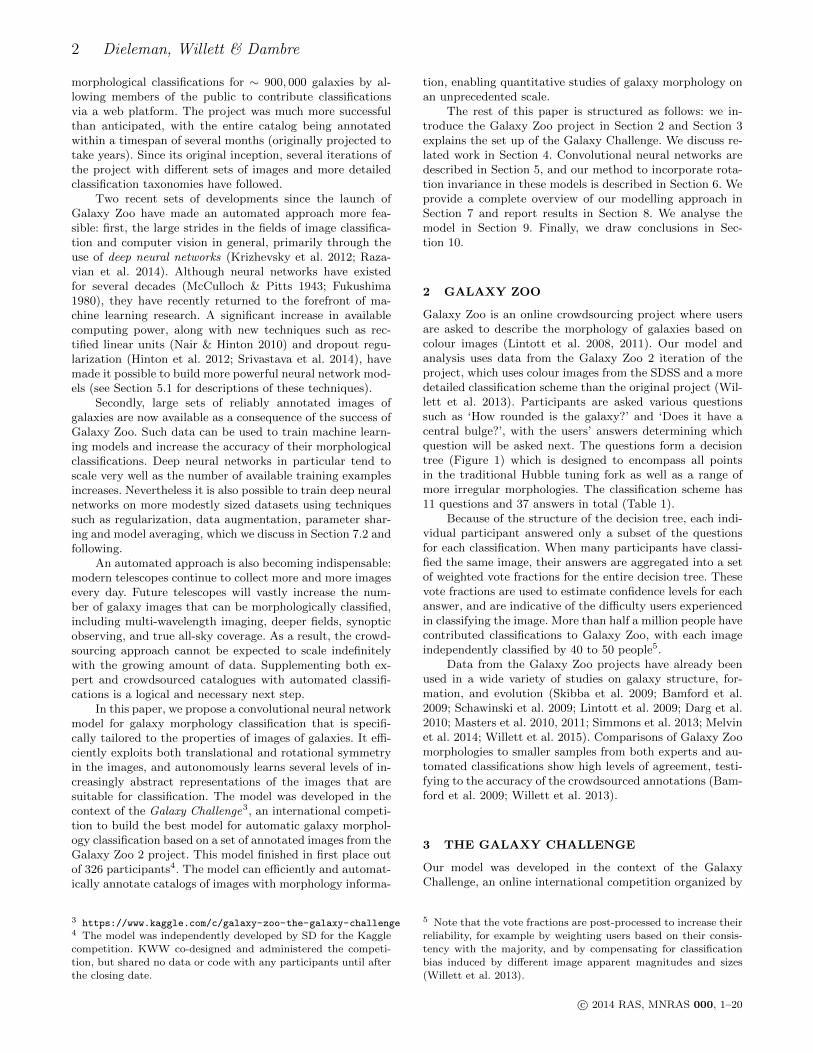
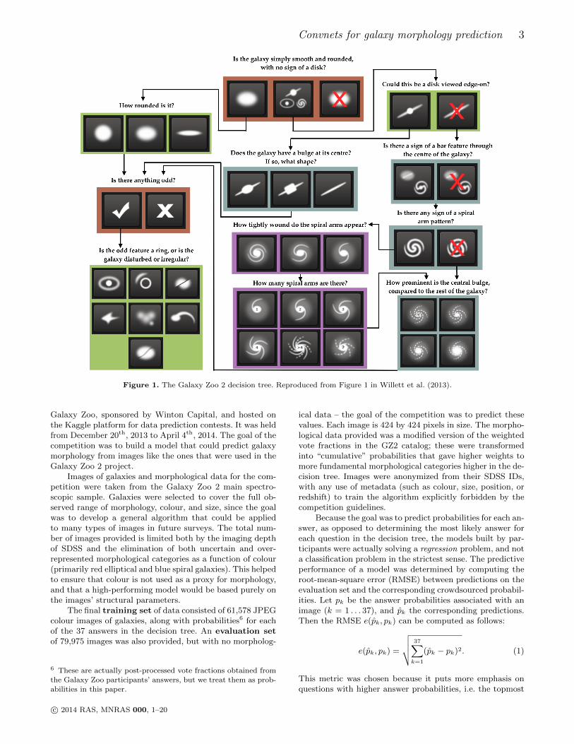
Galaxy Zoo is an online crowdsourcing project where usersare asked to describe the morphology of galaxies based oncolour images (Lintott et al. 2008, 2011). Our model andanalysis uses data from the Galaxy Zoo 2 iteration of theproject, which uses colour images from the SDSS and a moredetailed classification scheme than the original project (Wil-lett et al. 2013). Participants are asked various questionssuch as ‘How rounded is the galaxy?’ and ‘Does it have acentral bulge?’, with the users’ answers determining whichquestion will be asked next. The questions form a decisiontree (Figure 1) which is designed to encompass all pointsin the traditional Hubble tuning fork as well as a range ofmore irregular morphologies. The classification scheme has11 questions and 37 answers in total (Table 1).

Because of the structure of the decision tree, each indi-vidual participant answered only a subset of the questionsfor each classification. When many participants have classi-fied the same image, their answers are aggregated into a setof weighted vote fractions for the entire decision tree. Thesevote fractions are used to estimate confidence levels for eachanswer, and are indicative of the difficulty users experiencedin classifying the image. More than half a million people havecontributed classifications to Galaxy Zoo, with each imageindependently classified by 40 to 50 people5.

Data from the Galaxy Zoo projects have already beenused in a wide variety of studies on galaxy structure, for-mation, and evolution (Skibba et al. 2009; Bamford et al.2009; Schawinski et al. 2009; Lintott et al. 2009; Darg et al.2010; Masters et al. 2010, 2011; Simmons et al. 2013; Melvinet al. 2014; Willett et al. 2015). Comparisons of Galaxy Zoomorphologies to smaller samples from both experts and au-tomated classifications show high levels of agreement, testi-fying to the accuracy of the crowdsourced annotations (Bam-ford et al. 2009; Willett et al. 2013).

3 THE GALAXY CHALLENGE

Our model was developed in the context of the GalaxyChallenge, an online international competition organized by

5 Note that the vote fractions are post-processed to increase theirreliability, for example by weighting users based on their consis-tency with the majority, and by compensating for classification

bias induced by different image apparent magnitudes and sizes(Willett et al. 2013).

c© 2014 RAS, MNRAS 000, 1–20

Convnets for galaxy morphology prediction 3

Figure 1. The Galaxy Zoo 2 decision tree. Reproduced from Figure 1 in Willett et al. (2013).

Galaxy Zoo, sponsored by Winton Capital, and hosted onthe Kaggle platform for data prediction contests. It was heldfrom December 20th, 2013 to April 4th, 2014. The goal of thecompetition was to build a model that could predict galaxymorphology from images like the ones that were used in theGalaxy Zoo 2 project.

Images of galaxies and morphological data for the com-petition were taken from the Galaxy Zoo 2 main spectro-scopic sample. Galaxies were selected to cover the full ob-served range of morphology, colour, and size, since the goalwas to develop a general algorithm that could be appliedto many types of images in future surveys. The total num-ber of images provided is limited both by the imaging depthof SDSS and the elimination of both uncertain and over-represented morphological categories as a function of colour(primarily red elliptical and blue spiral galaxies). This helpedto ensure that colour is not used as a proxy for morphology,and that a high-performing model would be based purely onthe images’ structural parameters.

The final training set of data consisted of 61,578 JPEGcolour images of galaxies, along with probabilities6 for eachof the 37 answers in the decision tree. An evaluation setof 79,975 images was also provided, but with no morpholog-

6 These are actually post-processed vote fractions obtained from

the Galaxy Zoo participants’ answers, but we treat them as prob-abilities in this paper.

ical data – the goal of the competition was to predict thesevalues. Each image is 424 by 424 pixels in size. The morpho-logical data provided was a modified version of the weightedvote fractions in the GZ2 catalog; these were transformedinto “cumulative” probabilities that gave higher weights tomore fundamental morphological categories higher in the de-cision tree. Images were anonymized from their SDSS IDs,with any use of metadata (such as colour, size, position, orredshift) to train the algorithm explicitly forbidden by thecompetition guidelines.

Because the goal was to predict probabilities for each an-swer, as opposed to determining the most likely answer foreach question in the decision tree, the models built by par-ticipants were actually solving a regression problem, and nota classification problem in the strictest sense. The predictiveperformance of a model was determined by computing theroot-mean-square error (RMSE) between predictions on theevaluation set and the corresponding crowdsourced probabil-ities. Let pk be the answer probabilities associated with animage (k = 1 . . . 37), and pk the corresponding predictions.Then the RMSE e(pk, pk) can be computed as follows:

e(pk, pk) =

√√√√ 37∑k=1

(pk − pk)2. (1)

This metric was chosen because it puts more emphasis onquestions with higher answer probabilities, i.e. the topmost

c© 2014 RAS, MNRAS 000, 1–20

4 Dieleman, Willett & Dambre

question answers next

Q1Is the galaxy simply smooth and

rounded, with no sign of a disk?

A1.1 smooth Q7

A1.2 features or disk Q2

A1.3 star or artifact end

Q2Could this be a disk viewed

edge-on?

A2.1 yes Q9

A2.2 no Q3

Q3Is there a sign of a bar feature

through the centre of the galaxy?

A3.1 yes Q4

A3.2 no Q4

Q4Is there any sign of a spiral arm

pattern?

A4.1 yes Q10

A4.2 no Q5

Q5

How prominent is the central

bulge, compared with the rest of

the galaxy?

A5.1 no bulge Q6

A5.2 just noticeable Q6

A5.3 obvious Q6

A5.4 dominant Q6

Q6 Is there anything odd?A6.1 yes Q8

A6.2 no end

Q7 How rounded is it?

A7.1 completely round Q6

A7.2 in between Q6

A7.3 cigar-shaped Q6

Q8Is the odd feature a ring, or is the

galaxy disturbed or irregular?

A8.1 ring end

A8.2 lens or arc end

A8.3 disturbed end

A8.4 irregular end

A8.5 other end

A8.6 merger end

A8.7 dust lane end

Q9Does the galaxy have a bulge at its

centre? If so, what shape?

A9.1 rounded Q6

A9.2 boxy Q6

A9.3 no bulge Q6

Q10How tightly wound do the spiral

arms appear?

A10.1 tight Q11

A10.2 medium Q11

A10.3 loose Q11

Q11 How many spiral arms are there?

A11.1 1 Q5

A11.2 2 Q5

A11.3 3 Q5

A11.4 4 Q5

A11.5 more than four Q5

A11.6 can’t tell Q5

Table 1. All questions that can be asked about an image, with thecorresponding answers that participants can choose from. Ques-

tion 1 is the only one that is asked of every image. The final

column indicates the next question to be asked when a particularanswer is given. Reproduced from Table 2 in Willett et al. (2013).

questions in the decision tree, which correspond to broadermorphological categories.

The provided answer probabilities are derived fromcrowdsourced classifications, so they are somewhat noisy andbiased in certain ways. As a result, the predictive models thatwere built exhibited some of the same biases. In other words,they are models of how the crowd would classify images ofgalaxies, which may not necessarily correspond to the “true”morphology. An example of such a discrepancy is discussedin Section 9.

The models built by participants were evaluated asfollows. The Kaggle platform automatically computed twoscores based on a set of model predictions: a public score,computed on about 25% of the evaluation data, and a privatescore, computed on the other 75%. Public scores were im-mediately revealed during the course of the competition, butprivate scores were not revealed until after the competitionhad finished. The private score was used to determine thefinal ranking. Because the participants did not know whichevaluation images belonged to which set, they could not di-rectly optimize the private score, but were instead encour-

aged to build a predictive model that generalizes well to newimages.

4 RELATED WORK

Machine learning techniques, and artificial neural networksin particular, have been a popular tool in astronomy researchfor more than two decades. Neural networks were initiallyapplied for star-galaxy discrimination (Odewahn et al. 1992;Bertin 1994) and classification of galaxy spectra (Folkes et al.1996). More recently they have also been used for photomet-ric redshift estimation (Firth et al. 2003; Collister & Lahav2004).

Galaxy morphology classification is one of the mostwidespread applications of neural networks in astronomy.Most work in this domain proceeds by preprocessing thephotometric data and then extracting a limited set of hand-crafted features that are known to be discriminative, such asellipticity, concentration, surface brightness, and radii andlog-likelihood values measured from various types of radialprofiles (Storrie-Lombardi et al. 1992; Lahav et al. 1995;Naim et al. 1995; Lahav et al. 1996; Ball et al. 2004; Banerjiet al. 2010). Support vector machines (SVMs) have also beenapplied in this fashion (Huertas-Company et al. 2010).

Earlier work in this domain typically relied on muchsmaller datasets and used networks with very few trainableparameters (between 101 and 103). Modern network archi-tectures are capable of handling at least ∼ 107 parameters,allowing for more precise fits and a larger morphologicalclassification space. More recent work has profited from theavailability of larger training sets using data from surveyssuch as the SDSS (Banerji et al. 2010; Huertas-Companyet al. 2010).

Another recent trend is the use of general purpose im-age features, instead of features that are specific to galaxies:the WND-CHARM feature set (Orlov et al. 2008), originallydesigned for biological image analysis, has been applied togalaxy morphology classification in combination with near-est neighbour classifiers (Shamir 2009; Shamir et al. 2013;Kuminski et al. 2014).

Other approaches to this problem attempt to forgo anyform of handcrafted feature extraction by applying principalcomponent analysis (PCA) to preprocessed images in com-bination with a neural network (De La Calleja & Fuentes2004), or by applying kernel SVMs directly to raw pixel data(Polsterer et al. 2012).

Our approach differs from prior work in two main areas:

• Most prior work uses handcrafted features (e.g., WND-CHARM) that required expert knowledge and many hours ofengineering to develop. We work directly with raw pixel dataand our use of convolutional neural networks allows for a setof task-specific features to be learned from the data. Thenetworks learn hierarchies of features, which allow them todetect complex patterns in the images. Handcrafted featuresmostly rely on image statistics and very local pattern detec-tors, making it harder to recognize complex patterns. Fur-thermore, it is usually necessary to perform feature selectionbecause the handcrafted representations are highly redun-dant and many features are irrelevant for the task at hand.Although many other participants in the Galaxy Challenge

c© 2014 RAS, MNRAS 000, 1–20

Convnets for galaxy morphology prediction 5

used convolutional neural networks, there is little discussionof this approach in the astronomical literature.• Apart from the recent work of Kuminski et al. (2014),

whose algorithms are also trained on Galaxy Zoo data, mostresearch has focused on classifying galaxies into a limitednumber of classes (typically between 2 and 5), or predict-ing scalar values that are indicative of galaxy morphology(e.g., Hubble T-types). Since the classifications made byGalaxy Zoo users are much more fine-grained, the task thenetworks must solve is more challenging. Since many out-standing astrophysical questions require more detailed mor-phological data (such as the number and arrangements ofclumps into proto-galaxies, the relation between bar strengthand central star formation, link between merging activityand active black holes, etc.), development of models thatcan handle these more difficult tasks is crucial.

Our method for classifying galaxy morphology exploitsthe rotational symmetry of galaxy images; however, thereare other invariances and symmetries (besides translational)that may be exploited for convolutional neural networks.Bruna et al. (2013) define convolution operations over ar-bitrary graphs, generalizing from the typical grid of pixelsto other locally connected structures. Sifre & Mallat (2013)extract representations that are invariant to affine transfor-mations, based on scattering transforms. However, these rep-resentations are fixed (i.e., not learned from data), and notspecifically tuned for the task at hand, unlike the represen-tations learned by convolutional neural networks.

Mairal et al. (2014) propose to train convolutional neu-ral networks to approximate kernel feature maps, allowingfor the desired invariance properties to be encoded in thechoice of kernel, and subsequently learned. Gens & Domingos(2014) propose deep symmetry networks, a generalization ofconvolutional neural networks with the ability to form fea-ture maps over any symmetry group, rather than just thetranslation group. Our approach for exploiting rotationalsymmetry in the input images, described in Section 6, isquite similar in spirit to this work. The major advantage toour implementation is a demonstrably effective result at areasonable computational cost.

5 BACKGROUND

5.1 Deep learning

The idea of deep learning is to build models that representdata at multiple levels of abstraction, and can discover accu-rate representations autonomously from the data itself (Ben-gio 2007). Deep learning models consist of several layers ofprocessing that form a hierarchy: each subsequent layer ex-tracts a progressively more abstract representation of theinput data and builds upon the representation from the pre-vious layer, typically by computing a non-linear transforma-tion of its input. The parameters of these transformationsare optimized by training the model on a dataset.

A feed-forward neural network is an example of sucha model, where each layer consists of a number of units(or neurons) that compute a weighted linear combinationof the layer input, followed by an elementwise non-linearity.These weights constitute the model parameters. Let the vec-tor xn−1 be the input to layer n, Wn be a matrix of weights,

output

layer N (output)

xN = f(WNxN−1 + bN )

layer N − 1 (hidden)

xN−1 = f(WN−1xN−2 + bN−1)

layer 1 (hidden)x1 = f(W1x0 + b1)

input

· · ·

xN

xN−1

xN−2

x1

x0

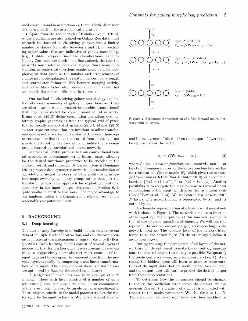
Figure 2. Schematic representation of a feed-forward neural net-work with N layers.

and bn be a vector of biases. Then the output of layer n canbe represented as the vector

xn = f(Wnxn−1 + bn), (2)

where f is the activation function, an elementwise non-linearfunction. Common choices for the activation function are lin-ear rectification [f(x) = max(x, 0)], which gives rise to recti-fied linear units (ReLUs; Nair & Hinton 2010), or a sigmoidalfunction [f(x) = (1 + e−x)−1 or f(x) = tanh(x)]. Anotherpossibility is to compute the maximum across several linearcombinations of the input, which gives rise to maxout units(Goodfellow et al. 2013). We will consider a network withN layers. The network input is represented by x0, and itsoutput by xN .

A schematic representation of a feed-forward neural net-work is shown in Figure 2. The network computes a functionof the input x0. The output xN of this function is a predic-tion of one or more quantities of interest. We will use t torepresent the desired output (target) corresponding to thenetwork input x0. The topmost layer of the network is re-ferred to as the output layer. All the other layers below itare hidden layers.

During training, the parameters of all layers of the net-work are jointly optimized to make the output xN approxi-mate the desired output t as closely as possible. We quantifythe prediction error using an error measure e(xN , t). As aresult, the hidden layers will learn to produce representa-tions of the input data that are useful for the task at hand,and the output layer will learn to predict the desired outputfrom these representations.

To determine how the parameters should be changedto reduce the prediction error across the dataset, we usegradient descent : the gradient of e(xN , t) is computed withrespect to the model parameters Wn, bn for n = 1 . . . N .The parameter values of each layer are then modified by

c© 2014 RAS, MNRAS 000, 1–20

6 Dieleman, Willett & Dambre

repeatedly taking small steps in the direction opposite tothe gradient:

Wn ←Wn − η∂e(xN , t)

∂Wn, (3)

bn ← bn − η∂e(xN , t)

∂bn. (4)

Here, η is the learning rate, a hyperparameter controlling thestep size.

Traditionally, models with many non-linear layers ofprocessing have not been commonly used because they weredifficult to train: gradient information would vanish as itpropagated through the layers, making it difficult to learnthe parameters of lower layers (Hochreiter et al. 2001). Prac-tical applications of neural networks were limited to modelswith one or two hidden layers. Since 2006, the invention ofseveral new techniques, along with a significant increase inavailable computing power, have made this task much morefeasible.

Initially unsupervised pre-training was proposed as amethod to facilitate training deeper networks (Hinton et al.2006). Single-layer unsupervised models (such as restrictedBoltzmann machines or auto-encoders (Bengio 2007)) arestacked on top of each other and trained, and the learnedparameters of these models are then used to initialize theparameters of a deep neural network. These are then fine-tuned using standard gradient descent. This initializationscheme makes it possible to largely avoid the vanishing gra-dient problem. Nair & Hinton (2010) and Glorot et al. (2011)proposed the use of rectified linear units (ReLUs) in deepneural networks. By replacing traditional activation func-tions with linear rectification, the vanishing gradient prob-lem was significantly reduced. This also makes pre-trainingunnecessary in most cases.

The introduction of dropout regularization (Hintonet al. 2012; Srivastava et al. 2014) has made it possible totrain larger networks with many more parameters. Dropoutis a regularization method that can be applied to a layer n byrandomly removing the output values of the previous layern − 1 (setting them to zero) with probability p. Typicallyp is chosen to be 0.5. The remaining values are rescaled bya factor of (1 − p)−1 to preserve the scale of the total in-put to each unit in layer n. For each training example thatis presented to the network, a different subset of values isremoved. During evaluation, no values are removed and norescaling is performed.

Dropout is an effective regularizer because it preventscoadaptation between units: each unit is forced to learn tobe useful by itself, because its utility cannot depend on thepresence of other units in the same layer (as they can beremoved at random).

5.2 Convolutional neural networks

Convolutional neural networks or convnets (Fukushima1980; LeCun et al. 1998) are a subclass of neural networkswith constrained connectivity patterns between some of thelayers. They can be used when the input data exhibits somekind of topological structure, like the ordering of image pix-els in a grid, or the temporal structure of an audio signal.

Convolutional neural networks contain two types of lay-

ers with restricted connectivity: convolutional layers andpooling layers. A convolutional layer takes a stack of featuremaps (e.g. the colour channels of an image) as input and con-volves each of these with a set of learnable filters to produce astack of output feature maps. This is efficiently implementedby replacing the matrix-vector product Wnxn−1 in Equa-tion 2 with a sum of convolutions. We represent the input oflayer n as a set of K matrices X

(k)n−1, with k = 1 . . .K. Each

of these matrices represents a different input feature map.The output feature maps X

(l)n , l = 1 . . . L are represented as

follows:

X(l)n = f

(K∑

k=1

W(k,l)n ∗X

(k)n−1 + b(l)n

). (5)

Here, ∗ represents the two-dimensional convolution opera-tion, the matrices W

(k,l)n represent the filters of layer n, and

b(l)n represents the bias for feature map l. Note that a feature

map X(l)n is obtained by computing a sum of K convolutions

with the feature maps of the previous layer. The bias b(l)n can

optionally be replaced by a matrix B(l)n , so that each spatial

position in the feature map has its own bias (‘untied’ bi-ases). This allows the sensitivity of the filters to vary acrossthe input.

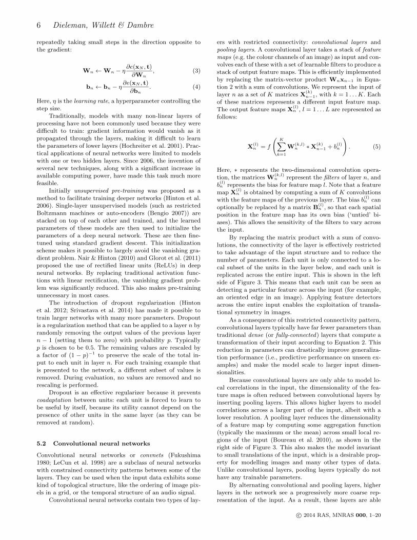
By replacing the matrix product with a sum of convo-lutions, the connectivity of the layer is effectively restrictedto take advantage of the input structure and to reduce thenumber of parameters. Each unit is only connected to a lo-cal subset of the units in the layer below, and each unit isreplicated across the entire input. This is shown in the leftside of Figure 3. This means that each unit can be seen asdetecting a particular feature across the input (for example,an oriented edge in an image). Applying feature detectorsacross the entire input enables the exploitation of transla-tional symmetry in images.

As a consequence of this restricted connectivity pattern,convolutional layers typically have far fewer parameters thantraditional dense (or fully-connected) layers that compute atransformation of their input according to Equation 2. Thisreduction in parameters can drastically improve generaliza-tion performance (i.e., predictive performance on unseen ex-amples) and make the model scale to larger input dimen-sionalities.

Because convolutional layers are only able to model lo-cal correlations in the input, the dimensionality of the fea-ture maps is often reduced between convolutional layers byinserting pooling layers. This allows higher layers to modelcorrelations across a larger part of the input, albeit with alower resolution. A pooling layer reduces the dimensionalityof a feature map by computing some aggregation function(typically the maximum or the mean) across small local re-gions of the input (Boureau et al. 2010), as shown in theright side of Figure 3. This also makes the model invariantto small translations of the input, which is a desirable prop-erty for modelling images and many other types of data.Unlike convolutional layers, pooling layers typically do nothave any trainable parameters.

By alternating convolutional and pooling layers, higherlayers in the network see a progressively more coarse rep-resentation of the input. As a result, these layers are able

c© 2014 RAS, MNRAS 000, 1–20

Convnets for galaxy morphology prediction 7

layer n− 1 layer n layer n + 1input convolutions pooling

X(k)n−1

X(l)n

X(l)n+1

W(k,l)n

Figure 3. A schematic overview of a convolutional layer followed by a pooling layer: each unit in the convolutional layer is connected toa local neighborhood in all feature maps of the previous layer. The pooling layer aggregates groups of neighboring units from the layer

below.

to model higher-level abstractions more easily because eachunit is able to see a larger part of the input.

Convolutional neural networks constitute the state ofthe art in many computer vision problems. Since their ef-fectiveness for large-scale image classification was demon-strated, they have been ubiquitous in computer vision re-search (Krizhevsky et al. 2012; Razavian et al. 2014; Szegedyet al. 2014; Simonyan & Zisserman 2014).

6 EXPLOITING ROTATIONAL SYMMETRY

The restricted connectivity patterns used in convolutionalneural networks drastically reduce the number of parametersrequired to model large images, by exploiting translationalsymmetry. However, there are many other types of symme-tries that occur in images. For images of galaxies, rotatingan image should not affect its morphological classification.This rotational symmetry is exploited by applying the sameset of feature detectors to various rotated versions of the in-put. This further increases parameter sharing, which has apositive effect on generalization performance.

Whereas convolutions provide an efficient way to exploittranslational symmetry, applying the same filter to multiplerotated versions of the input requires explicitly instantiatingthese versions. Additionally, rotating an image by an anglethat is not a multiple of 90◦ requires interpolation and re-sults in an image whose edges are not aligned with the rowsand columns of the pixel grid. These complications makeexploiting rotational symmetry more challenging.

We note that the original Galaxy Zoo project experi-mented with crowdsourced classifications of galaxies in whichthe images were both vertically and diagonally mirrored.Land et al. (2008) showed that the raw votes had an excessof 2.5% for S-wise (anticlockwise) spiral galaxies over Z-wise(clockwise) galaxies. Since this effect was seen in both theraw and mirrored images, it was interpreted as a bias due topreferences in the human brain, rather than as a true excessin the number of apparent S-wise spirals in the Universe.The existence of such a directional bias in the brain wasdemonstrated by Gori et al. (2006). The Galaxy Zoo 2 prob-abilities do not contain any structures related to handedness

or rotation-variant quantities, and no rotational or transla-tional biases have yet been discovered in the data. If suchbiases do exist, however, this would presumably reduce thepredictive power of the model since the assumption of rota-tional invariance to the output probabilities would no longerapply.

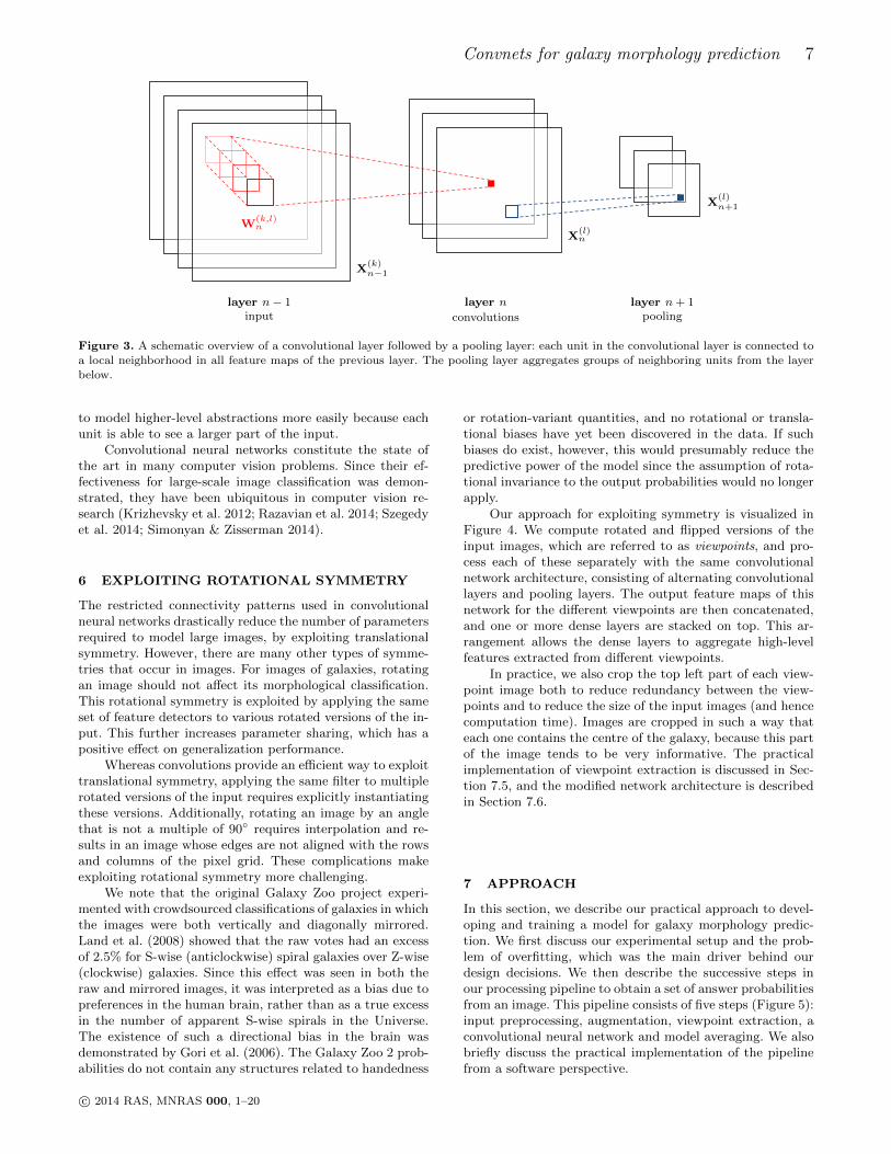
Our approach for exploiting symmetry is visualized inFigure 4. We compute rotated and flipped versions of theinput images, which are referred to as viewpoints, and pro-cess each of these separately with the same convolutionalnetwork architecture, consisting of alternating convolutionallayers and pooling layers. The output feature maps of thisnetwork for the different viewpoints are then concatenated,and one or more dense layers are stacked on top. This ar-rangement allows the dense layers to aggregate high-levelfeatures extracted from different viewpoints.

In practice, we also crop the top left part of each view-point image both to reduce redundancy between the view-points and to reduce the size of the input images (and hencecomputation time). Images are cropped in such a way thateach one contains the centre of the galaxy, because this partof the image tends to be very informative. The practicalimplementation of viewpoint extraction is discussed in Sec-tion 7.5, and the modified network architecture is describedin Section 7.6.

7 APPROACH

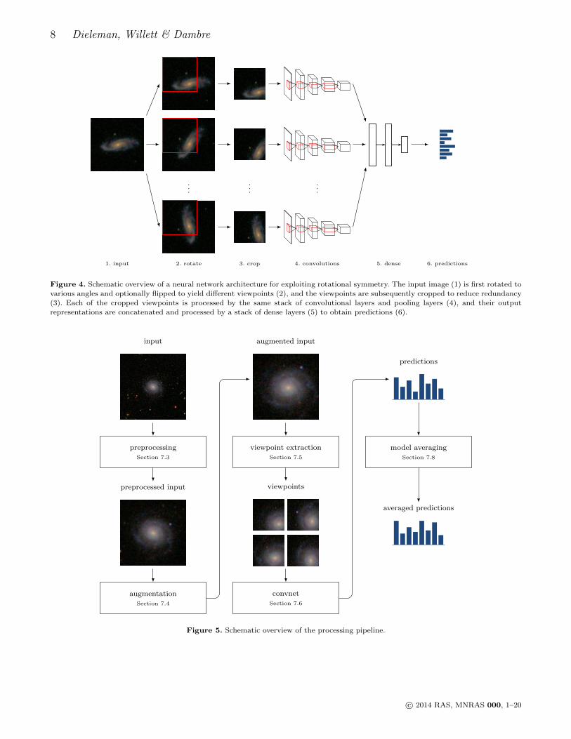
In this section, we describe our practical approach to devel-oping and training a model for galaxy morphology predic-tion. We first discuss our experimental setup and the prob-lem of overfitting, which was the main driver behind ourdesign decisions. We then describe the successive steps inour processing pipeline to obtain a set of answer probabilitiesfrom an image. This pipeline consists of five steps (Figure 5):input preprocessing, augmentation, viewpoint extraction, aconvolutional neural network and model averaging. We alsobriefly discuss the practical implementation of the pipelinefrom a software perspective.

c© 2014 RAS, MNRAS 000, 1–20

8 Dieleman, Willett & Dambre

..

....

.

..

1. input 2. rotate 3. crop 4. convolutions 5. dense 6. predictions

Figure 4. Schematic overview of a neural network architecture for exploiting rotational symmetry. The input image (1) is first rotated to

various angles and optionally flipped to yield different viewpoints (2), and the viewpoints are subsequently cropped to reduce redundancy(3). Each of the cropped viewpoints is processed by the same stack of convolutional layers and pooling layers (4), and their output

representations are concatenated and processed by a stack of dense layers (5) to obtain predictions (6).

input augmented input

predictions

preprocessing

Section 7.3

viewpoint extraction

Section 7.5

model averaging

Section 7.8

preprocessed input viewpoints

averaged predictions

augmentation

Section 7.4

convnetSection 7.6

Figure 5. Schematic overview of the processing pipeline.

c© 2014 RAS, MNRAS 000, 1–20

Convnets for galaxy morphology prediction 9

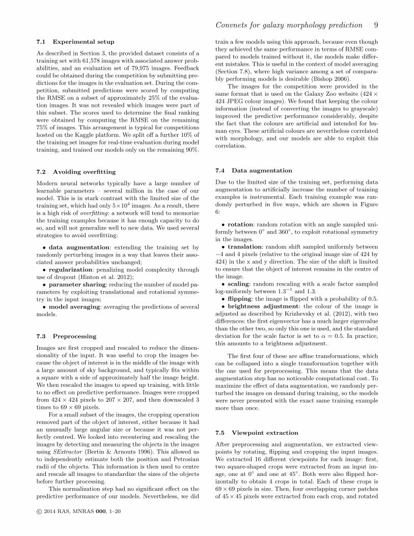
7.1 Experimental setup

As described in Section 3, the provided dataset consists of atraining set with 61,578 images with associated answer prob-abilities, and an evaluation set of 79,975 images. Feedbackcould be obtained during the competition by submitting pre-dictions for the images in the evaluation set. During the com-petition, submitted predictions were scored by computingthe RMSE on a subset of approximately 25% of the evalua-tion images. It was not revealed which images were part ofthis subset. The scores used to determine the final rankingwere obtained by computing the RMSE on the remaining75% of images. This arrangement is typical for competitionshosted on the Kaggle platform. We split off a further 10% ofthe training set images for real-time evaluation during modeltraining, and trained our models only on the remaining 90%.

7.2 Avoiding overfitting

Modern neural networks typically have a large number oflearnable parameters – several million in the case of ourmodel. This is in stark contrast with the limited size of thetraining set, which had only 5×104 images. As a result, thereis a high risk of overfitting : a network will tend to memorizethe training examples because it has enough capacity to doso, and will not generalize well to new data. We used severalstrategies to avoid overfitting:

• data augmentation: extending the training set byrandomly perturbing images in a way that leaves their asso-ciated answer probabilities unchanged;• regularization: penalizing model complexity through

use of dropout (Hinton et al. 2012);• parameter sharing: reducing the number of model pa-

rameters by exploiting translational and rotational symme-try in the input images;• model averaging: averaging the predictions of several

models.

7.3 Preprocessing

Images are first cropped and rescaled to reduce the dimen-sionality of the input. It was useful to crop the images be-cause the object of interest is in the middle of the image witha large amount of sky background, and typically fits withina square with a side of approximately half the image height.We then rescaled the images to speed up training, with littleto no effect on predictive performance. Images were croppedfrom 424 × 424 pixels to 207 × 207, and then downscaled 3times to 69× 69 pixels.

For a small subset of the images, the cropping operationremoved part of the object of interest, either because it hadan unusually large angular size or because it was not per-fectly centred. We looked into recentering and rescaling theimages by detecting and measuring the objects in the imagesusing SExtractor (Bertin & Arnouts 1996). This allowed usto independently estimate both the position and Petrosianradii of the objects. This information is then used to centreand rescale all images to standardize the sizes of the objectsbefore further processing.

This normalization step had no significant effect on thepredictive performance of our models. Nevertheless, we did

train a few models using this approach, because even thoughthey achieved the same performance in terms of RMSE com-pared to models trained without it, the models make differ-ent mistakes. This is useful in the context of model averaging(Section 7.8), where high variance among a set of compara-bly performing models is desirable (Bishop 2006).

The images for the competition were provided in thesame format that is used on the Galaxy Zoo website (424×424 JPEG colour images). We found that keeping the colourinformation (instead of converting the images to grayscale)improved the predictive performance considerably, despitethe fact that the colours are artificial and intended for hu-man eyes. These artificial colours are nevertheless correlatedwith morphology, and our models are able to exploit thiscorrelation.

7.4 Data augmentation

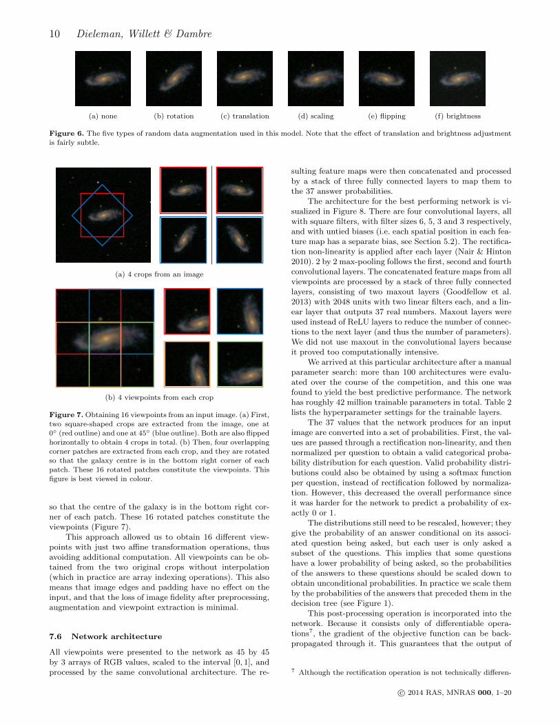
Due to the limited size of the training set, performing dataaugmentation to artificially increase the number of trainingexamples is instrumental. Each training example was ran-domly perturbed in five ways, which are shown in Figure6:

• rotation: random rotation with an angle sampled uni-formly between 0◦ and 360◦, to exploit rotational symmetryin the images.• translation: random shift sampled uniformly between

−4 and 4 pixels (relative to the original image size of 424 by424) in the x and y direction. The size of the shift is limitedto ensure that the object of interest remains in the centre ofthe image.• scaling: random rescaling with a scale factor sampled

log-uniformly between 1.3−1 and 1.3.• flipping: the image is flipped with a probability of 0.5.• brightness adjustment: the colour of the image is

adjusted as described by Krizhevsky et al. (2012), with twodifferences: the first eigenvector has a much larger eigenvaluethan the other two, so only this one is used, and the standarddeviation for the scale factor is set to α = 0.5. In practice,this amounts to a brightness adjustment.

The first four of these are affine transformations, whichcan be collapsed into a single transformation together withthe one used for preprocessing. This means that the dataaugmentation step has no noticeable computational cost. Tomaximize the effect of data augmentation, we randomly per-turbed the images on demand during training, so the modelswere never presented with the exact same training examplemore than once.

7.5 Viewpoint extraction

After preprocessing and augmentation, we extracted view-points by rotating, flipping and cropping the input images.We extracted 16 different viewpoints for each image: first,two square-shaped crops were extracted from an input im-age, one at 0◦ and one at 45◦. Both were also flipped hor-izontally to obtain 4 crops in total. Each of these crops is69× 69 pixels in size. Then, four overlapping corner patchesof 45× 45 pixels were extracted from each crop, and rotated

c© 2014 RAS, MNRAS 000, 1–20

10 Dieleman, Willett & Dambre

(a) none (b) rotation (c) translation (d) scaling (e) flipping (f) brightness

Figure 6. The five types of random data augmentation used in this model. Note that the effect of translation and brightness adjustment

is fairly subtle.

(a) 4 crops from an image

(b) 4 viewpoints from each crop

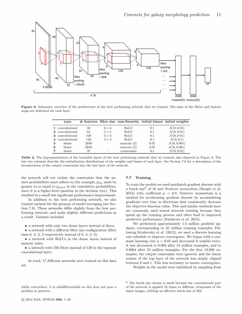
Figure 7. Obtaining 16 viewpoints from an input image. (a) First,

two square-shaped crops are extracted from the image, one at0◦ (red outline) and one at 45◦ (blue outline). Both are also flipped

horizontally to obtain 4 crops in total. (b) Then, four overlappingcorner patches are extracted from each crop, and they are rotated

so that the galaxy centre is in the bottom right corner of each

patch. These 16 rotated patches constitute the viewpoints. Thisfigure is best viewed in colour.

so that the centre of the galaxy is in the bottom right cor-ner of each patch. These 16 rotated patches constitute theviewpoints (Figure 7).

This approach allowed us to obtain 16 different view-points with just two affine transformation operations, thusavoiding additional computation. All viewpoints can be ob-tained from the two original crops without interpolation(which in practice are array indexing operations). This alsomeans that image edges and padding have no effect on theinput, and that the loss of image fidelity after preprocessing,augmentation and viewpoint extraction is minimal.

7.6 Network architecture

All viewpoints were presented to the network as 45 by 45by 3 arrays of RGB values, scaled to the interval [0, 1], andprocessed by the same convolutional architecture. The re-

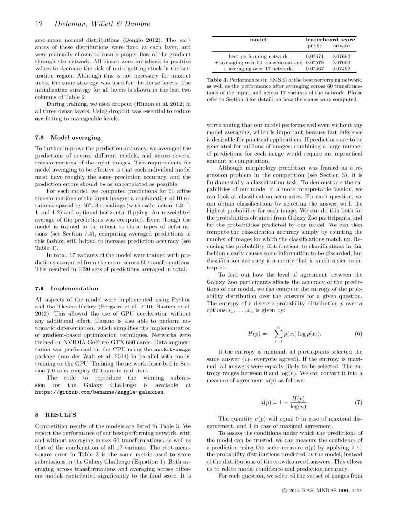
sulting feature maps were then concatenated and processedby a stack of three fully connected layers to map them tothe 37 answer probabilities.

The architecture for the best performing network is vi-sualized in Figure 8. There are four convolutional layers, allwith square filters, with filter sizes 6, 5, 3 and 3 respectively,and with untied biases (i.e. each spatial position in each fea-ture map has a separate bias, see Section 5.2). The rectifica-tion non-linearity is applied after each layer (Nair & Hinton2010). 2 by 2 max-pooling follows the first, second and fourthconvolutional layers. The concatenated feature maps from allviewpoints are processed by a stack of three fully connectedlayers, consisting of two maxout layers (Goodfellow et al.2013) with 2048 units with two linear filters each, and a lin-ear layer that outputs 37 real numbers. Maxout layers wereused instead of ReLU layers to reduce the number of connec-tions to the next layer (and thus the number of parameters).We did not use maxout in the convolutional layers becauseit proved too computationally intensive.

We arrived at this particular architecture after a manualparameter search: more than 100 architectures were evalu-ated over the course of the competition, and this one wasfound to yield the best predictive performance. The networkhas roughly 42 million trainable parameters in total. Table 2lists the hyperparameter settings for the trainable layers.

The 37 values that the network produces for an inputimage are converted into a set of probabilities. First, the val-ues are passed through a rectification non-linearity, and thennormalized per question to obtain a valid categorical proba-bility distribution for each question. Valid probability distri-butions could also be obtained by using a softmax functionper question, instead of rectification followed by normaliza-tion. However, this decreased the overall performance sinceit was harder for the network to predict a probability of ex-actly 0 or 1.

The distributions still need to be rescaled, however; theygive the probability of an answer conditional on its associ-ated question being asked, but each user is only asked asubset of the questions. This implies that some questionshave a lower probability of being asked, so the probabilitiesof the answers to these questions should be scaled down toobtain unconditional probabilities. In practice we scale themby the probabilities of the answers that preceded them in thedecision tree (see Figure 1).

This post-processing operation is incorporated into thenetwork. Because it consists only of differentiable opera-tions7, the gradient of the objective function can be back-propagated through it. This guarantees that the output of

7 Although the rectification operation is not technically differen-

c© 2014 RAS, MNRAS 000, 1–20

Convnets for galaxy morphology prediction 11

3 (RGB)32

64

128128

2048maxout(2)

2048maxout(2)

37

x 16

…

…

…

…

Maxpooling= 20x20

Maxpooling= 8x8

Maxpooling= 2x2

45

45

40

40

16

16

6

6

4

4

6

6

5

5 3

3 3

3

Figure 8. Schematic overview of the architecture of the best performing network that we trained. The sizes of the filters and feature

maps are indicated for each layer.

type # features filter size non-linearity initial biases initial weights

1 convolutional 32 6× 6 ReLU 0.1 N (0, 0.01)2 convolutional 64 5× 5 ReLU 0.1 N (0, 0.01)3 convolutional 128 3× 3 ReLU 0.1 N (0, 0.01)4 convolutional 128 3× 3 ReLU 0.1 N (0, 0.1)5 dense 2048 – maxout (2) 0.01 N (0, 0.001)6 dense 2048 – maxout (2) 0.01 N (0, 0.001)7 dense 37 – constraints 0.1 N (0, 0.01)

Table 2. The hyperparameters of the trainable layers of the best performing network that we trained, also depicted in Figure 8. The

last two columns describe the initialization distributions of the weights and biases of each layer. See Section 7.6 for a description of theincorporation of the output constraints into the last layer of the network.

the network will not violate the constraints that the an-swer probabilities must adhere to (for example, pbar must begreater to or equal to pspiral in the cumulative probabilities,since it is a higher-level question in the decision tree). Thisresulted in a small but significant performance improvement.

In addition to the best performing network, we alsotrained variants for the purpose of model averaging (see Sec-tion 7.8). These networks differ slightly from the best per-forming network, and make slightly different predictions asa result. Variants included:

• a network with only two dense layers instead of three;• a network with a different filter size configuration (filter

sizes 8, 4, 3, 3 respectively instead of 6, 5, 3, 3);• a network with ReLUs in the dense layers instead of

maxout units;• a network with 256 filters instead of 128 in the topmost

convolutional layer.

In total, 17 different networks were trained on this dataset.

tiable everywhere, it is subdifferentiable so this does not pose a

problem in practice.

7.7 Training

To train the models we used minibatch gradient descent witha batch size8 of 16 and Nesterov momentum (Bengio et al.2013) with coefficient µ = 0.9. Nesterov momentum is amethod for accelerating gradient descent by accumulatinggradients over time in directions that consistently decreasethe objective function value. This and similar methods haveare commonly used neural network training because theyspeed up the training process and often lead to improvedpredictive performance (Sutskever et al. 2013).

We performed approximately 1.5 million gradient up-dates, corresponding to 25 million training examples. Fol-lowing Krizhevsky et al. (2012), we used a discrete learningrate schedule to improve convergence. We began with a con-stant learning rate η = 0.04 and decreased it tenfold twice:it was decreased to 0.004 after 18 million examples, and to0.0004 after 23 million examples. For the first 10,000 ex-amples, the output constraints were ignored, and the linearoutput of the top layer of the network was simply clippedbetween 0 and 1. This was necessary to ensure convergence.

Weights in the model were initialized by sampling from

8 The batch size chosen is small because the convolutional part

of the network is applied 16 times to different viewpoints of the

input images, yielding an effective batch size of 256.

c© 2014 RAS, MNRAS 000, 1–20

12 Dieleman, Willett & Dambre

zero-mean normal distributions (Bengio 2012). The vari-ances of these distributions were fixed at each layer, andwere manually chosen to ensure proper flow of the gradientthrough the network. All biases were initialized to positivevalues to decrease the risk of units getting stuck in the sat-uration region. Although this is not necessary for maxoutunits, the same strategy was used for the dense layers. Theinitialization strategy for all layers is shown in the last twocolumns of Table 2.

During training, we used dropout (Hinton et al. 2012) inall three dense layers. Using dropout was essential to reduceoverfitting to manageable levels.

7.8 Model averaging

To further improve the prediction accuracy, we averaged thepredictions of several different models, and across severaltransformations of the input images. Two requirements formodel averaging to be effective is that each individual modelmust have roughly the same prediction accuracy, and theprediction errors should be as uncorrelated as possible.

For each model, we computed predictions for 60 affinetransformations of the input images: a combination of 10 ro-tations, spaced by 36◦, 3 rescalings (with scale factors 1.2−1,1 and 1.2) and optional horizontal flipping. An unweightedaverage of the predictions was computed. Even though themodel is trained to be robust to these types of deforma-tions (see Section 7.4), computing averaged predictions inthis fashion still helped to increase prediction accuracy (seeTable 3).

In total, 17 variants of the model were trained with pre-dictions computed from the mean across 60 transformations.This resulted in 1020 sets of predictions averaged in total.

7.9 Implementation

All aspects of the model were implemented using Pythonand the Theano library (Bergstra et al. 2010; Bastien et al.2012). This allowed the use of GPU acceleration withoutany additional effort. Theano is also able to perform au-tomatic differentiation, which simplifies the implementationof gradient-based optimization techniques. Networks weretrained on NVIDIA GeForce GTX 680 cards. Data augmen-tation was performed on the CPU using the scikit-image

package (van der Walt et al. 2014) in parallel with modeltraining on the GPU. Training the network described in Sec-tion 7.6 took roughly 67 hours in real time.

The code to reproduce the winning submis-sion for the Galaxy Challenge is available athttps://github.com/benanne/kaggle-galaxies.

8 RESULTS

Competition results of the models are listed in Table 3. Wereport the performance of our best performing network, withand without averaging across 60 transformations, as well asthat of the combination of all 17 variants. The root-mean-square error in Table 3 is the same metric used to scoresubmissions in the Galaxy Challenge (Equation 1). Both av-eraging across transformations and averaging across differ-ent models contributed significantly to the final score. It is

model leaderboard scorepublic private

best performing network 0.07671 0.07693+ averaging over 60 transformations 0.07579 0.07603

+ averaging over 17 networks 0.07467 0.07492

Table 3. Performance (in RMSE) of the best performing network,

as well as the performance after averaging across 60 transforma-tions of the input, and across 17 variants of the network. Please

refer to Section 3 for details on how the scores were computed.

worth noting that our model performs well even without anymodel averaging, which is important because fast inferenceis desirable for practical applications. If predictions are to begenerated for millions of images, combining a large numberof predictions for each image would require an impracticalamount of computation.

Although morphology prediction was framed as a re-gression problem in the competition (see Section 3), it isfundamentally a classification task. To demonstrate the ca-pabilities of our model in a more interpretable fashion, wecan look at classification accuracies. For each question, wecan obtain classifications by selecting the answer with thehighest probability for each image. We can do this both forthe probabilities obtained from Galaxy Zoo participants, andfor the probabilities predicted by our model. We can thencompute the classification accuracy simply by counting thenumber of images for which the classifications match up. Re-ducing the probability distributions to classifications in thisfashion clearly causes some information to be discarded, butclassification accuracy is a metric that is much easier to in-terpret.

To find out how the level of agreement between theGalaxy Zoo participants affects the accuracy of the predic-tions of our model, we can compute the entropy of the prob-ability distribution over the answers for a given question.The entropy of a discrete probability distribution p over noptions x1, . . . , xn is given by:

H(p) = −n∑

i=1

p(xi) log p(xi). (6)

If the entropy is minimal, all participants selected thesame answer (i.e. everyone agreed). If the entropy is maxi-mal, all answers were equally likely to be selected. The en-tropy ranges between 0 and log(n). We can convert it into ameasure of agreement a(p) as follows:

a(p) = 1− H(p)

log(n). (7)

The quantity a(p) will equal 0 in case of maximal dis-agreement, and 1 in case of maximal agreement.

To assess the conditions under which the predictions ofthe model can be trusted, we can measure the confidence ofa prediction using the same measure a(p) by applying it tothe probability distributions predicted by the model, insteadof the distributions of the crowdsourced answers. This allowsus to relate model confidence and prediction accuracy.

For each question, we selected the subset of images from

c© 2014 RAS, MNRAS 000, 1–20

Convnets for galaxy morphology prediction 13

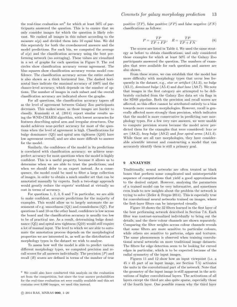
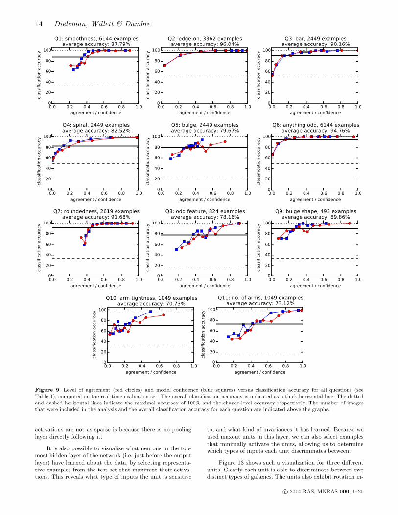
the real-time evaluation set9 for which at least 50% of par-ticipants answered the question. This is to ensure that weonly consider images for which the question is likely rele-vant. We ranked all images in this subset according to themeasure a(p) and divided them into 10 equal bins. We didthis seperately for both the crowdsourced answers and themodel predictions. For each bin, we computed the averageof a(p) and the classification accuracy using the best per-forming network (no averaging). These values are visualizedin a set of graphs for each question in Figure 9. The redcircles show classification accuracy versus agreement. Theblue squares show classification accuracy versus model con-fidence. The classification accuracy across the entire subsetis also shown as a thick horizontal line. The dashed hori-zontal lines indicate the maximal accuracy of 100% and thechance-level accuracy, which depends on the number of op-tions. The number of images in each subset and the overallclassification accuracy are indicated above the graphs.

For all questions, the classification accuracy tapers offas the level of agreement between Galaxy Zoo participantsdecreases. This makes sense, as those images are harder toclassify. Kuminski et al. (2014) report similar results us-ing the WND-CHARM algorithm, with lowest accuracies forfeatures describing spiral arm and irregular structures. Ourmodel achieves near-perfect accuracy for most of the ques-tions when the level of agreement is high. Classifications forbulge dominance (Q5) and spiral arm tightness (Q10) havelow agreement overall, and are also more difficult to answerfor the model.

Similarly, the confidence of the model in its predictionsis correlated with classification accuracy: we achieve near-perfect accuracy for most questions when the model is highlyconfident. This is a useful property, because it allows us todetermine when we are able to trust the predictions, andwhen we should defer to an expert instead. As a conse-quence, the model could be used to filter a large collectionof images, in order to obtain a much smaller set that can beannotated manually by experts. Such a two-stage approachwould greatly reduce the experts’ workload at virtually nocost in terms of accuracy.

For questions 1, 2, 3, 6 and 7 in particular, we are ableto make confident, accurate predictions for the majority ofexamples. This would allow us to largely automate the as-sessment of e.g. smoothness (Q1) and roundedness (Q7). Forquestions 5 and 10 on the other hand, confidence is low acrossthe board and the classification accuracy is usually too lowto be of practical use. As a result, determining bulge domi-nance (Q5) and spiral arm tightness (Q10) would still requirea lot of manual input. The level to which we are able to auto-mate the annotation process depends on the morphologicalproperties we are interested in, as well as the distribution ofmorphology types in the dataset we wish to analyse.

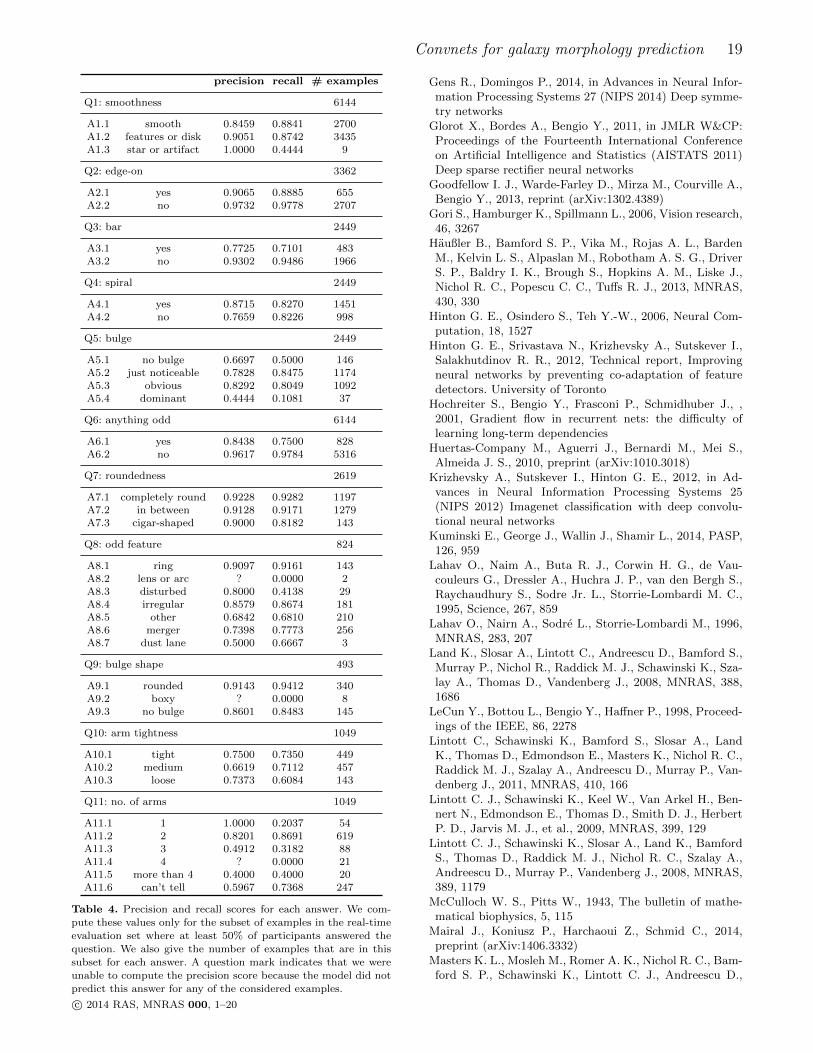
To assess how well the model is able to predict variousdifferent morphology types, we computed precision and re-call scores for all answers individually. The precision (P ) andrecall (R) scores are defined in terms of the number of true

9 We could also have conducted this analysis on the evaluationset from the competition, but since the true answer probabilities

for the real-time evaluation set were readily available and this setcontains over 6,000 images, we used this instead.

positive (TP ), false positive (FP ) and false negative (FN)classifications as follows:

P =TP

TP + FP, R =

TP

TP + FN. (8)

The scores are listed in Table 4. We used the same strat-egy as before to obtain classifications, and only consideredthose examples for which at least 50% of the Galaxy Zooparticipants answered the question. The numbers of exam-ples that were available for each question and answer arealso shown.

From these scores, we can establish that the model hasmore difficulty with morphology types that occur less fre-quently in the dataset, e.g., star or artifact (A1.3), no bulge(A5.1), dominant bulge (A5.4) and dust lane (A8.7). We notethat images in the first category are attempted to be deli-brately excluded from the Galaxy Zoo data set via flags inthe SDSS pipeline. Both the precision and recall scores areaffected, so this effect cannot be attributed entirely to a biastowards more common morphologies. However, recall is gen-erally affected more strongly than precision, which indicatesthat the model is more conservative in predicting rare mor-phology types. For a few very rare answers, we were unableto compute precision scores because the model never pre-dicted them for the examples that were considered: lens orarc (A8.2), boxy bulge (A9.2) and four spiral arms (A11.4).While these are all rare morphologies, they have consider-able scientific interest and constructing a model that canaccurately identify them is still a primary goal.

9 ANALYSIS

Traditionally, neural networks are often treated as blackboxes that perform some complicated and uninterpretablesequence of computations that yield a good approximationto the desired output. However, analysing the parametersof a trained model can be very informative, and sometimeseven leads to new insights about the problem the network istrying to solve (Zeiler & Fergus 2014). This is especially truefor convolutional neural networks trained on images, wherethe first-layer filters can be interpreted visually.

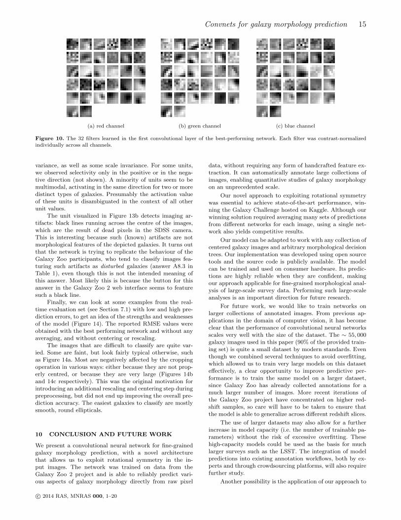
Figure 10 shows the 32 filters learned in the first layer ofthe best performing network described in Section 7.6. Eachfilter was contrast-normalized individually to bring out thedetails, and the three colour channels are shown separately.Comparing the filter weights across colour channels revealsthat some filters are more sensitive to particular colours,while others are sensitive to patterns, edges and textures.The same phenomenon is observed when training convolu-tional neural networks on more traditional image datasets.The filters for edge detection seem to be looking for curvededges in particular, which is to be expected because of theradial symmetry of the input images.

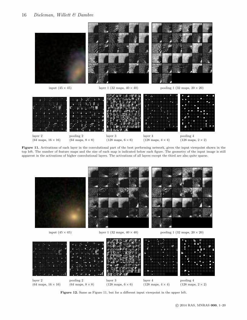
Figures 11 and 12 show how an input viewpoint (i.e. a45 × 45 part of an input image, see Section 7.5) activatesthe units in the convolutional part of the network. Note thatthe geometry of the input image is still apparent in the acti-vations of higher convolutional layers. The activations of alllayers except the third are also quite sparse, especially thoseof the fourth layer. One possible reason why the third layer

c© 2014 RAS, MNRAS 000, 1–20

14 Dieleman, Willett & Dambre

0.0 0.2 0.4 0.6 0.8 1.0

agreement / confidence

0

20

40

60

80

100

class

ific

ati

on a

ccura

cyQ1: smoothness, 6144 examples

average accuracy: 87.79%

0.0 0.2 0.4 0.6 0.8 1.0

agreement / confidence

0

20

40

60

80

100

class

ific

ati

on a

ccura

cy

Q2: edge-on, 3362 examplesaverage accuracy: 96.04%

0.0 0.2 0.4 0.6 0.8 1.0

agreement / confidence

0

20

40

60

80

100

class

ific

ati

on a

ccura

cy

Q3: bar, 2449 examplesaverage accuracy: 90.16%

0.0 0.2 0.4 0.6 0.8 1.0

agreement / confidence

0

20

40

60

80

100

class

ific

ati

on a

ccura

cy

Q4: spiral, 2449 examplesaverage accuracy: 82.52%

0.0 0.2 0.4 0.6 0.8 1.0

agreement / confidence

0

20

40

60

80

100

class

ific

ati

on a

ccura

cy

Q5: bulge, 2449 examplesaverage accuracy: 79.67%

0.0 0.2 0.4 0.6 0.8 1.0

agreement / confidence

0

20

40

60

80

100

class

ific

ati

on a

ccura

cy

Q6: anything odd, 6144 examplesaverage accuracy: 94.76%

0.0 0.2 0.4 0.6 0.8 1.0

agreement / confidence

0

20

40

60

80

100

class

ific

ati

on a

ccura

cy

Q7: roundedness, 2619 examplesaverage accuracy: 91.68%

0.0 0.2 0.4 0.6 0.8 1.0

agreement / confidence

0

20

40

60

80

100

class

ific

ati

on a

ccura

cy

Q8: odd feature, 824 examplesaverage accuracy: 78.16%

0.0 0.2 0.4 0.6 0.8 1.0

agreement / confidence

0

20

40

60

80

100

class

ific

ati

on a

ccura

cy

Q9: bulge shape, 493 examplesaverage accuracy: 89.86%

0.0 0.2 0.4 0.6 0.8 1.0

agreement / confidence

0

20

40

60

80

100

class

ific

ati

on a

ccura

cy

Q10: arm tightness, 1049 examplesaverage accuracy: 70.73%

0.0 0.2 0.4 0.6 0.8 1.0

agreement / confidence

0

20

40

60

80

100

class

ific

ati

on a

ccura

cy

Q11: no. of arms, 1049 examplesaverage accuracy: 73.12%

Figure 9. Level of agreement (red circles) and model confidence (blue squares) versus classification accuracy for all questions (seeTable 1), computed on the real-time evaluation set. The overall classification accuracy is indicated as a thick horizontal line. The dottedand dashed horizontal lines indicate the maximal accuracy of 100% and the chance-level accuracy respectively. The number of imagesthat were included in the analysis and the overall classification accuracy for each question are indicated above the graphs.

activations are not as sparse is because there is no poolinglayer directly following it.

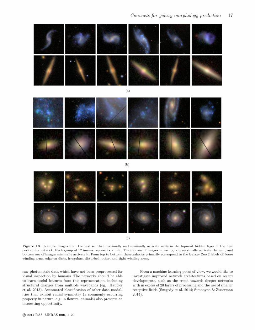
It is also possible to visualize what neurons in the top-most hidden layer of the network (i.e. just before the outputlayer) have learned about the data, by selecting representa-tive examples from the test set that maximize their activa-tions. This reveals what type of inputs the unit is sensitive

to, and what kind of invariances it has learned. Because weused maxout units in this layer, we can also select examplesthat minimally activate the units, allowing us to determinewhich types of inputs each unit discriminates between.

Figure 13 shows such a visualization for three differentunits. Clearly each unit is able to discriminate between twodistinct types of galaxies. The units also exhibit rotation in-

c© 2014 RAS, MNRAS 000, 1–20

Convnets for galaxy morphology prediction 15

(a) red channel (b) green channel (c) blue channel

Figure 10. The 32 filters learned in the first convolutional layer of the best-performing network. Each filter was contrast-normalized

individually across all channels.

variance, as well as some scale invariance. For some units,we observed selectivity only in the positive or in the nega-tive direction (not shown). A minority of units seem to bemultimodal, activating in the same direction for two or moredistinct types of galaxies. Presumably the activation valueof these units is disambiguated in the context of all otherunit values.

The unit visualized in Figure 13b detects imaging ar-tifacts: black lines running across the centre of the images,which are the result of dead pixels in the SDSS camera.This is interesting because such (known) artifacts are notmorphological features of the depicted galaxies. It turns outthat the network is trying to replicate the behaviour of theGalaxy Zoo participants, who tend to classify images fea-turing such artifacts as disturbed galaxies (answer A8.3 inTable 1), even though this is not the intended meaning ofthis answer. Most likely this is because the button for thisanswer in the Galaxy Zoo 2 web interface seems to featuresuch a black line.

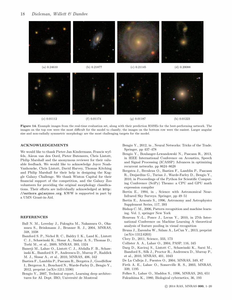
Finally, we can look at some examples from the real-time evaluation set (see Section 7.1) with low and high pre-diction errors, to get an idea of the strengths and weaknessesof the model (Figure 14). The reported RMSE values wereobtained with the best performing network and without anyaveraging, and without centering or rescaling.

The images that are difficult to classify are quite var-ied. Some are faint, but look fairly typical otherwise, suchas Figure 14a. Most are negatively affected by the croppingoperation in various ways: either because they are not prop-erly centred, or because they are very large (Figures 14band 14c respectively). This was the original motivation forintroducing an additional rescaling and centering step duringpreprocessing, but did not end up improving the overall pre-diction accuracy. The easiest galaxies to classify are mostlysmooth, round ellipticals.

10 CONCLUSION AND FUTURE WORK

We present a convolutional neural network for fine-grainedgalaxy morphology prediction, with a novel architecturethat allows us to exploit rotational symmetry in the in-put images. The network was trained on data from theGalaxy Zoo 2 project and is able to reliably predict vari-ous aspects of galaxy morphology directly from raw pixel

data, without requiring any form of handcrafted feature ex-traction. It can automatically annotate large collections ofimages, enabling quantitative studies of galaxy morphologyon an unprecedented scale.

Our novel approach to exploiting rotational symmetrywas essential to achieve state-of-the-art performance, win-ning the Galaxy Challenge hosted on Kaggle. Although ourwinning solution required averaging many sets of predictionsfrom different networks for each image, using a single net-work also yields competitive results.

Our model can be adapted to work with any collection ofcentered galaxy images and arbitrary morphological decisiontrees. Our implementation was developed using open sourcetools and the source code is publicly available. The modelcan be trained and used on consumer hardware. Its predic-tions are highly reliable when they are confident, makingour approach applicable for fine-grained morphological anal-ysis of large-scale survey data. Performing such large-scaleanalyses is an important direction for future research.

For future work, we would like to train networks onlarger collections of annotated images. From previous ap-plications in the domain of computer vision, it has becomeclear that the performance of convolutional neural networksscales very well with the size of the dataset. The ∼ 55, 000galaxy images used in this paper (90% of the provided train-ing set) is quite a small dataset by modern standards. Eventhough we combined several techniques to avoid overfitting,which allowed us to train very large models on this dataseteffectively, a clear opportunity to improve predictive per-formance is to train the same model on a larger dataset,since Galaxy Zoo has already collected annotations for amuch larger number of images. More recent iterations ofthe Galaxy Zoo project have concentrated on higher red-shift samples, so care will have to be taken to ensure thatthe model is able to generalize across different redshift slices.

The use of larger datasets may also allow for a furtherincrease in model capacity (i.e. the number of trainable pa-rameters) without the risk of excessive overfitting. Thesehigh-capacity models could be used as the basis for muchlarger surveys such as the LSST. The integration of modelpredictions into existing annotation workflows, both by ex-perts and through crowdsourcing platforms, will also requirefurther study.

Another possibility is the application of our approach to

c© 2014 RAS, MNRAS 000, 1–20

16 Dieleman, Willett & Dambre

input (45× 45) layer 1 (32 maps, 40× 40) pooling 1 (32 maps, 20× 20)

layer 2

(64 maps, 16× 16)

pooling 2

(64 maps, 8× 8)

layer 3

(128 maps, 6× 6)

layer 4

(128 maps, 4× 4)

pooling 4

(128 maps, 2× 2)

Figure 11. Activations of each layer in the convolutional part of the best performing network, given the input viewpoint shown in the

top left. The number of feature maps and the size of each map is indicated below each figure. The geometry of the input image is stillapparent in the activations of higher convolutional layers. The activations of all layers except the third are also quite sparse.

input (45× 45) layer 1 (32 maps, 40× 40) pooling 1 (32 maps, 20× 20)

layer 2

(64 maps, 16× 16)

pooling 2

(64 maps, 8× 8)

layer 3

(128 maps, 6× 6)

layer 4

(128 maps, 4× 4)

pooling 4

(128 maps, 2× 2)

Figure 12. Same as Figure 11, but for a different input viewpoint in the upper left.

c© 2014 RAS, MNRAS 000, 1–20

Convnets for galaxy morphology prediction 17

(a)

(b)

(c)

Figure 13. Example images from the test set that maximally and minimally activate units in the topmost hidden layer of the best

performing network. Each group of 12 images represents a unit. The top row of images in each group maximally activate the unit, andbottom row of images minimally activate it. From top to bottom, these galaxies primarily correspond to the Galaxy Zoo 2 labels of: loosewinding arms, edge-on disks, irregulars, disturbed, other, and tight winding arms.

raw photometric data which have not been preprocessed forvisual inspection by humans. The networks should be ableto learn useful features from this representation, includingstructural changes from multiple wavebands (eg, Haußleret al. 2013). Automated classification of other data modal-ities that exhibit radial symmetry (a commonly occurringproperty in nature, e.g. in flowers, animals) also presents aninteresting opportunity.

From a machine learning point of view, we would like toinvestigate improved network architectures based on recentdevelopments, such as the trend towards deeper networkswith in excess of 20 layers of processing and the use of smallerreceptive fields (Szegedy et al. 2014; Simonyan & Zisserman2014).

c© 2014 RAS, MNRAS 000, 1–20

18 Dieleman, Willett & Dambre

(a) 0.24610 (b) 0.21877 (c) 0.21145 (d) 0.20088

(e) 0.01112 (f) 0.01174 (g) 0.01187 (h) 0.01223

Figure 14. Example images from the real-time evaluation set, along with their prediction RMSEs for the best-performing network. The

images on the top row were the most difficult for the model to classify; the images on the bottom row were the easiest. Larger angular

size and non-radially symmetric morphology are the most challenging targets for the model.

ACKNOWLEDGEMENTS

We would like to thank Pieter-Jan Kindermans, Francis wyf-fels, Aaron van den Oord, Pieter Buteneers, Chris Lintott,Philip Marshall and the anonymous reviewer for their valu-able feedback. We would like to acknowledge Joyce Noah-Vanhoucke, Chris Lintott, David Harvey, Thomas Kitchingand Philip Marshall for their help in designing the Kag-gle Galaxy Challenge. We thank Winton Capital for theirfinancial support of the competition, and the Galaxy Zoovolunteers for providing the original morphology classifica-tions. Their efforts are individually acknowledged at http:

//authors.galaxyzoo.org. KWW is supported in part bya UMN Grant-in-Aid.

REFERENCES

Ball N. M., Loveday J., Fukugita M., Nakamura O., Oka-mura S., Brinkmann J., Brunner R. J., 2004, MNRAS,348, 1038

Bamford S. P., Nichol R. C., Baldry I. K., Land K., LintottC. J., Schawinski K., Slosar A., Szalay A. S., Thomas D.,Torki M., et al., 2009, MNRAS, 393, 1324

Banerji M., Lahav O., Lintott C. J., Abdalla F. B., Schaw-inski K., Bamford S. P., Andreescu D., Murray P., RaddickM. J., Slosar A., et al., 2010, MNRAS, 406, 342

Bastien F., Lamblin P., Pascanu R., Bergstra J., GoodfellowI., Bergeron A., Bouchard N., Warde-Farley D., Bengio Y.,2012, preprint (arXiv:1211.5590)

Bengio Y., 2007, Technical report, Learning deep architec-tures for AI. Dept. IRO, Universite de Montreal

Bengio Y., 2012, in , Neural Networks: Tricks of the Trade.Springer, pp 437–478

Bengio Y., Boulanger-Lewandowski N., Pascanu R., 2013,in IEEE International Conference on Acoustics, Speechand Signal Processing (ICASSP) Advances in optimizingrecurrent networks. pp 8624–8628

Bergstra J., Breuleux O., Bastien F., Lamblin P., PascanuR., Desjardins G., Turian J., Warde-Farley D., Bengio Y.,2010, in Proceedings of the Python for Scientific Comput-ing Conference (SciPy) Theano: a CPU and GPU mathexpression compiler

Bertin E., 1994, in , Science with Astronomical Near-Infrared Sky Surveys. Springer, pp 49–51

Bertin E., Arnouts S., 1996, Astronomy and AstrophysicsSupplement Series, 117, 393

Bishop C. M., 2006, Pattern recognition and machine learn-ing. Vol. 1, springer New York

Boureau Y.-L., Ponce J., Lecun Y., 2010, in 27th Inter-national Conference on Machine Learning A theoreticalanalysis of feature pooling in visual recognition

Bruna J., Zaremba W., Szlam A., LeCun Y., 2013, preprint(arXiv:1312.6203)

Clery D., 2011, Science, 333, 173

Collister A. A., Lahav O., 2004, PASP, 116, 345

Darg D., Kaviraj S., Lintott C., Schawinski K., Sarzi M.,Bamford S., Silk J., Proctor R., Andreescu D., Murray P.,et al., 2010, MNRAS, 401, 1043

De La Calleja J., Fuentes O., 2004, MNRAS, 349, 87

Firth A. E., Lahav O., Somerville R. S., 2003, MNRAS,339, 1195

Folkes S., Lahav O., Maddox S., 1996, MNRAS, 283, 651

Fukushima K., 1980, Biological cybernetics, 36, 193

c© 2014 RAS, MNRAS 000, 1–20

Convnets for galaxy morphology prediction 19

precision recall # examples

Q1: smoothness 6144

A1.1 smooth 0.8459 0.8841 2700A1.2 features or disk 0.9051 0.8742 3435A1.3 star or artifact 1.0000 0.4444 9

Q2: edge-on 3362

A2.1 yes 0.9065 0.8885 655A2.2 no 0.9732 0.9778 2707

Q3: bar 2449

A3.1 yes 0.7725 0.7101 483A3.2 no 0.9302 0.9486 1966

Q4: spiral 2449

A4.1 yes 0.8715 0.8270 1451A4.2 no 0.7659 0.8226 998

Q5: bulge 2449

A5.1 no bulge 0.6697 0.5000 146A5.2 just noticeable 0.7828 0.8475 1174A5.3 obvious 0.8292 0.8049 1092A5.4 dominant 0.4444 0.1081 37

Q6: anything odd 6144

A6.1 yes 0.8438 0.7500 828A6.2 no 0.9617 0.9784 5316

Q7: roundedness 2619

A7.1 completely round 0.9228 0.9282 1197A7.2 in between 0.9128 0.9171 1279A7.3 cigar-shaped 0.9000 0.8182 143

Q8: odd feature 824

A8.1 ring 0.9097 0.9161 143A8.2 lens or arc ? 0.0000 2A8.3 disturbed 0.8000 0.4138 29A8.4 irregular 0.8579 0.8674 181A8.5 other 0.6842 0.6810 210A8.6 merger 0.7398 0.7773 256A8.7 dust lane 0.5000 0.6667 3

Q9: bulge shape 493

A9.1 rounded 0.9143 0.9412 340A9.2 boxy ? 0.0000 8A9.3 no bulge 0.8601 0.8483 145

Q10: arm tightness 1049

A10.1 tight 0.7500 0.7350 449A10.2 medium 0.6619 0.7112 457A10.3 loose 0.7373 0.6084 143

Q11: no. of arms 1049

A11.1 1 1.0000 0.2037 54A11.2 2 0.8201 0.8691 619A11.3 3 0.4912 0.3182 88A11.4 4 ? 0.0000 21A11.5 more than 4 0.4000 0.4000 20A11.6 can’t tell 0.5967 0.7368 247

Table 4. Precision and recall scores for each answer. We com-pute these values only for the subset of examples in the real-timeevaluation set where at least 50% of participants answered the

question. We also give the number of examples that are in thissubset for each answer. A question mark indicates that we were

unable to compute the precision score because the model did notpredict this answer for any of the considered examples.

Gens R., Domingos P., 2014, in Advances in Neural Infor-mation Processing Systems 27 (NIPS 2014) Deep symme-try networks

Glorot X., Bordes A., Bengio Y., 2011, in JMLR W&CP:Proceedings of the Fourteenth International Conferenceon Artificial Intelligence and Statistics (AISTATS 2011)Deep sparse rectifier neural networks

Goodfellow I. J., Warde-Farley D., Mirza M., Courville A.,Bengio Y., 2013, reprint (arXiv:1302.4389)

Gori S., Hamburger K., Spillmann L., 2006, Vision research,46, 3267

Haußler B., Bamford S. P., Vika M., Rojas A. L., BardenM., Kelvin L. S., Alpaslan M., Robotham A. S. G., DriverS. P., Baldry I. K., Brough S., Hopkins A. M., Liske J.,Nichol R. C., Popescu C. C., Tuffs R. J., 2013, MNRAS,430, 330

Hinton G. E., Osindero S., Teh Y.-W., 2006, Neural Com-putation, 18, 1527

Hinton G. E., Srivastava N., Krizhevsky A., Sutskever I.,Salakhutdinov R. R., 2012, Technical report, Improvingneural networks by preventing co-adaptation of featuredetectors. University of Toronto

Hochreiter S., Bengio Y., Frasconi P., Schmidhuber J., ,2001, Gradient flow in recurrent nets: the difficulty oflearning long-term dependencies

Huertas-Company M., Aguerri J., Bernardi M., Mei S.,Almeida J. S., 2010, preprint (arXiv:1010.3018)

Krizhevsky A., Sutskever I., Hinton G. E., 2012, in Ad-vances in Neural Information Processing Systems 25(NIPS 2012) Imagenet classification with deep convolu-tional neural networks

Kuminski E., George J., Wallin J., Shamir L., 2014, PASP,126, 959

Lahav O., Naim A., Buta R. J., Corwin H. G., de Vau-couleurs G., Dressler A., Huchra J. P., van den Bergh S.,Raychaudhury S., Sodre Jr. L., Storrie-Lombardi M. C.,1995, Science, 267, 859

Lahav O., Nairn A., Sodre L., Storrie-Lombardi M., 1996,MNRAS, 283, 207

Land K., Slosar A., Lintott C., Andreescu D., Bamford S.,Murray P., Nichol R., Raddick M. J., Schawinski K., Sza-lay A., Thomas D., Vandenberg J., 2008, MNRAS, 388,1686

LeCun Y., Bottou L., Bengio Y., Haffner P., 1998, Proceed-ings of the IEEE, 86, 2278

Lintott C., Schawinski K., Bamford S., Slosar A., LandK., Thomas D., Edmondson E., Masters K., Nichol R. C.,Raddick M. J., Szalay A., Andreescu D., Murray P., Van-denberg J., 2011, MNRAS, 410, 166

Lintott C. J., Schawinski K., Keel W., Van Arkel H., Ben-nert N., Edmondson E., Thomas D., Smith D. J., HerbertP. D., Jarvis M. J., et al., 2009, MNRAS, 399, 129

Lintott C. J., Schawinski K., Slosar A., Land K., BamfordS., Thomas D., Raddick M. J., Nichol R. C., Szalay A.,Andreescu D., Murray P., Vandenberg J., 2008, MNRAS,389, 1179

McCulloch W. S., Pitts W., 1943, The bulletin of mathe-matical biophysics, 5, 115

Mairal J., Koniusz P., Harchaoui Z., Schmid C., 2014,preprint (arXiv:1406.3332)

Masters K. L., Mosleh M., Romer A. K., Nichol R. C., Bam-ford S. P., Schawinski K., Lintott C. J., Andreescu D.,

c© 2014 RAS, MNRAS 000, 1–20

20 Dieleman, Willett & Dambre

Campbell H. C., Crowcroft B., et al., 2010, MNRAS, 405,783

Masters K. L., Nichol R. C., Hoyle B., Lintott C., BamfordS. P., Edmondson E. M., Fortson L., Keel W. C., Schaw-inski K., Smith A. M., et al., 2011, MNRAS, 411, 2026

Melvin T., Masters K., Lintott C., Nichol R. C., SimmonsB., Bamford S. P., Casteels K. R. V., Cheung E., Edmond-son E. M., Fortson L., Schawinski K., Skibba R. A., SmithA. M., Willett K. W., 2014, MNRAS

Naim A., Lahav O., Sodre L., Storrie-Lombardi M., 1995,MNRAS, 275, 567

Nair V., Hinton G. E., 2010, in Proceedings of the 27th In-ternational Conference on Machine Learning (ICML-10)Rectified linear units improve restricted boltzmann ma-chines

Odewahn S., Stockwell E., Pennington R., Humphreys R.,Zumach W., 1992, in , Digitised Optical Sky Surveys.Springer, pp 215–224

Orlov N., Shamir L., Macura T., Johnston J., Eckley D. M.,Goldberg I. G., 2008, Pattern recognition letters, 29, 1684

Polsterer K. L., Gieseke F., Kramer O., 2012, in Astronom-ical Data Analysis Software and Systems XXI Vol. 461,Galaxy classification without feature extraction. p. 561

Razavian A. S., Azizpour H., Sullivan J., Carlsson S., 2014,preprint (arXiv:1403.6382)

Schawinski K., Lintott C., Thomas D., Sarzi M., AndreescuD., Bamford S. P., Kaviraj S., Khochfar S., Land K., Mur-ray P., et al., 2009, MNRAS, 396, 818

Shamir L., 2009, MNRAS, 399, 1367Shamir L., Holincheck A., Wallin J., 2013, Astronomy andComputing, 2, 67

Sifre L., Mallat S., 2013, in IEEE Conference on ComputerVision and Pattern Recognition (CVPR) Rotation, scalingand deformation invariant scattering for texture discrimi-nation. pp 1233–1240

Simmons B. D., Lintott C., Schawinski K., Moran E. C.,Han A., Kaviraj S., Masters K. L., Urry C. M., WillettK. W., Bamford S. P., Nichol R. C., 2013, MNRAS, 429,2199

Simonyan K., Zisserman A., 2014, preprint(arXiv:1409.1556)

Skibba R. A., Bamford S. P., Nichol R. C., Lintott C. J.,Andreescu D., Edmondson E. M., Murray P., RaddickM. J., Schawinski K., Slosar A., Szalay A. S., ThomasD., Vandenberg J., 2009, MNRAS, 399, 966

Srivastava N., Hinton G., Krizhevsky A., Sutskever I.,Salakhutdinov R., 2014, Journal of Machine Learning Re-search, 15, 1929

Storrie-Lombardi M., Lahav O., Sodre L., Storrie-LombardiL., 1992, MNRAS, 259, 8P

Sutskever I., Martens J., Dahl G., Hinton G., 2013, in Pro-ceedings of the 30th International Conference on MachineLearning (ICML-13) On the importance of initializationand momentum in deep learning. pp 1139–1147

Szegedy C., Liu W., Jia Y., Sermanet P., Reed S.,Anguelov D., Erhan D., Vanhoucke V., Rabinovich A.,2014, preprint (arXiv:1409.4842)

van der Walt S., Schonberger J. L., Nunez-Iglesias J.,Boulogne F., Warner J. D., Yager N., Gouillart E., YuT., 2014, Technical report, scikit-image: Image processingin Python. PeerJ PrePrints

Willett K. W., Lintott C. J., Bamford S. P., Masters K. L.,

Simmons B. D., Casteels K. R., Edmondson E. M., FortsonL. F., Kaviraj S., Keel W. C., et al., 2013, MNRAS, 435,2835

Willett K. W., Schawinski K., Simmons B. D., MastersK. L., Skibba R. A., Kaviraj S., Melvin T., Wong O. I.,Nichol R. C., Cheung E., Lintott C. J., Fortson L., 2015

Zeiler M. D., Fergus R., 2014, in , Computer Vision–ECCV2014. Springer, pp 818–833

This paper has been typeset from a TEX/ LATEX file preparedby the author.

c© 2014 RAS, MNRAS 000, 1–20