Erwin V. ZaretskyGlenn Research Center, Cleveland, Ohio

Rolling Bearing Life Prediction, Theory, and Application

NASA/TP—2013-215305/REV1

November 2016

This Revised Copy, numbered as NASA/TP—2013-215305/REV1, November 2016, supersedesthe previous version, NASA/TP—2013-215305, March 2013, in its entirety.

https://ntrs.nasa.gov/search.jsp?R=20160013905 2020-01-29T00:54:06+00:00Z

NASA STI Program . . . in Profi le

Since its founding, NASA has been dedicated to the advancement of aeronautics and space science. The NASA Scientifi c and Technical Information (STI) Program plays a key part in helping NASA maintain this important role.

The NASA STI Program operates under the auspices of the Agency Chief Information Offi cer. It collects, organizes, provides for archiving, and disseminates NASA’s STI. The NASA STI Program provides access to the NASA Technical Report Server—Registered (NTRS Reg) and NASA Technical Report Server—Public (NTRS) thus providing one of the largest collections of aeronautical and space science STI in the world. Results are published in both non-NASA channels and by NASA in the NASA STI Report Series, which includes the following report types: • TECHNICAL PUBLICATION. Reports of

completed research or a major signifi cant phase of research that present the results of NASA programs and include extensive data or theoretical analysis. Includes compilations of signifi cant scientifi c and technical data and information deemed to be of continuing reference value. NASA counter-part of peer-reviewed formal professional papers, but has less stringent limitations on manuscript length and extent of graphic presentations.

• TECHNICAL MEMORANDUM. Scientifi c

and technical fi ndings that are preliminary or of specialized interest, e.g., “quick-release” reports, working papers, and bibliographies that contain minimal annotation. Does not contain extensive analysis.

• CONTRACTOR REPORT. Scientifi c and technical fi ndings by NASA-sponsored contractors and grantees.

• CONFERENCE PUBLICATION. Collected papers from scientifi c and technical conferences, symposia, seminars, or other meetings sponsored or co-sponsored by NASA.

• SPECIAL PUBLICATION. Scientifi c,

technical, or historical information from NASA programs, projects, and missions, often concerned with subjects having substantial public interest.

• TECHNICAL TRANSLATION. English-

language translations of foreign scientifi c and technical material pertinent to NASA’s mission.

For more information about the NASA STI program, see the following:

• Access the NASA STI program home page at http://www.sti.nasa.gov

• E-mail your question to help@sti.nasa.gov • Fax your question to the NASA STI

Information Desk at 757-864-6500

• Telephone the NASA STI Information Desk at 757-864-9658 • Write to:

NASA STI Program Mail Stop 148 NASA Langley Research Center Hampton, VA 23681-2199

Erwin V. ZaretskyGlenn Research Center, Cleveland, Ohio

Rolling Bearing Life Prediction, Theory, and Application

NASA/TP—2013-215305/REV1

November 2016

This Revised Copy, numbered as NASA/TP—2013-215305/REV1, November 2016, supersedesthe previous version, NASA/TP—2013-215305, March 2013, in its entirety.

National Aeronautics andSpace Administration

Glenn Research CenterCleveland, Ohio 44135

Available from

Level of Review: This material has been technically reviewed by technical management.

Revised Copy

This Revised Copy, numbered as NASA/TP—2013-215305/REV1, November 2016, supersedes the previous version, NASA/TP—2013-215305, March 2013, in its entirety.

Figures 27 and 28 have been changed.

Tracking No. has changed.

Report Documentation page has been removed.

NASA STI ProgramMail Stop 148NASA Langley Research CenterHampton, VA 23681-2199

National Technical Information Service5285 Port Royal RoadSpringfi eld, VA 22161

703-605-6000

This report is available in electronic form at http://www.sti.nasa.gov/ and http://ntrs.nasa.gov/

Trade names and trademarks are used in this report for identifi cation only. Their usage does not constitute an offi cial endorsement, either expressed or implied, by the National Aeronautics and

Space Administration.

This work was sponsored by the Fundamental Aeronautics Program at the NASA Glenn Research Center.

NASA/TP—2013-215305/REV1 iii

Contents

Summary........................................................................................................................................................................ 1 Introduction ................................................................................................................................................................... 1 Bearing Life Theory ...................................................................................................................................................... 2 

Foundation for Bearing Life Prediction .................................................................................................................. 2 Hertz Contact Stress Theory ............................................................................................................................ 2 Equivalent Load .............................................................................................................................................. 3 Fatigue Limit ................................................................................................................................................... 3 L10 Life ............................................................................................................................................................ 4 Linear Damage Rule ........................................................................................................................................ 5 

Weibull Analysis .................................................................................................................................................... 5 Weibull Distribution Function ......................................................................................................................... 5 Weibull Fracture Strength Model .................................................................................................................... 6 

Bearing Life Models ...................................................................................................................................................... 7 Weibull Fatigue Life Model ................................................................................................................................... 7 Lundberg-Palmgren Model .................................................................................................................................... 9 

Strict Series Reliability .................................................................................................................................. 10 Dynamic Load Capacity, CD ......................................................................................................................... 13 

Ioannides-Harris Model ........................................................................................................................................ 15 Zaretsky Model ..................................................................................................................................................... 16 

Ball and Roller Set Life ................................................................................................................................. 17 Ball-Race Conformity Effects ....................................................................................................................... 20 Deep-Groove Ball Bearings .......................................................................................................................... 23 Angular-Contact Ball Bearings ..................................................................................................................... 23 

Stress Effects ............................................................................................................................................................... 25 Hertz Stress-Life Relation .................................................................................................................................... 25 Residual and Hoop Stresses .................................................................................................................................. 29 

Comparison of Bearing Life Models ........................................................................................................................... 31 Comparing Life Data With Predictions ....................................................................................................................... 32 

Bearing Life Factors ............................................................................................................................................. 32 Bearing Life Variation .......................................................................................................................................... 33 Weibull Slope Variation ....................................................................................................................................... 38 

Turboprop Gearbox Case Study .................................................................................................................................. 38 Analysis ................................................................................................................................................................ 39 

Bearing Life Analysis .................................................................................................................................... 39 Gear Life Analysis ........................................................................................................................................ 41 Gearbox System Life ..................................................................................................................................... 41 

Gearbox Field Data .............................................................................................................................................. 42 Reevaluation of Bearing Load-Life Exponent p ................................................................................................... 42 

Appendix A.—Fatigue Limit ....................................................................................................................................... 45 Appendix B.—Derivation of Weibull Distribution Function ...................................................................................... 49 Appendix C.—Derivation of Strict Series Reliability ................................................................................................. 51 Appendix D.—Contact (Hertz) Stress ......................................................................................................................... 53 References ................................................................................................................................................................... 54 

NASA/TP—2013-215305/REV1 1

Rolling Bearing Life Prediction, Theory, and Application

Erwin V. Zaretsky National Aeronautics and Space Administration

Glenn Research Center Cleveland, Ohio 44135

Summary

A tutorial is presented outlining the evolution, theory, and application of rolling-element bearing life prediction from that of A. Palmgren, 1924; W. Weibull, 1939; G. Lundberg and A. Palmgren, 1947 and 1952; E. Ioannides and T. Harris, 1985; and E. Zaretsky, 1987. Comparisons are made between these life models. The Ioannides-Harris model without a fatigue limit is identical to the Lundberg-Palmgren model. The Weibull model is similar to that of Zaretsky if the exponents are chosen to be identical. Both the load-life and Hertz stress-life relations of Weibull, Lundberg and Palmgren, and Ioannides and Harris reflect a strong dependence on the Weibull slope. The Zaretsky model decouples the dependence of the critical shear stress-life relation from the Weibull slope. This results in a nominal variation of the Hertz stress-life exponent.

For 9th- and 8th-power Hertz stress-life exponents for ball and roller bearings, respectively, the Lundberg-Palmgren model best predicts life. However, for 12th- and 10th-power relations reflected by modern bearing steels, the Zaretsky model based on the Weibull equation is superior. Under the range of stresses examined, the use of a fatigue limit would suggest that (for most operating conditions under which a rolling-element bearing will operate) the bearing will not fail from classical rolling-element fatigue. Realistically, this is not the case. The use of a fatigue limit will significantly overpre-dict life over a range of normal operating Hertz stresses. (The use of ISO 281:2007 with a fatigue limit in these calculations would result in a bearing life approaching infinity.) Since the predicted lives of rolling-element bearings are high, the problem can become one of undersizing a bearing for a particular application.

Rules had been developed to distinguish and compare predicted lives with those actually obtained. Based upon field and test results of 51 ball and roller bearing sets, 98 percent of these bearing sets had acceptable life results using the Lundberg-Palmgren equations with life adjustment factors to predict bearing life. That is, they had lives equal to or greater than that predicted.

The Lundberg-Palmgren model was used to predict the life of a commercial turboprop gearbox. The life prediction was compared with the field lives of 64 gearboxes. From these results, the roller bearing lives exhibited a load-life exponent of 5.2, which correlated with the Zaretsky model. The use of the ANSI/ABMA and ISO standards load-life exponent of 10/3 to predict roller bearing life is not reflective of modern roller bearings and will underpredict bearing lives.

Introduction

By the close of the 19th century, the rolling-element bearing industry began to focus on sizing of ball and roller bearings for specific applications and determining bearing life and reliabil-ity. In 1896, R. Stribeck (Ref. 1) in Germany began fatigue testing full-scale rolling-element bearings. J. Goodman (Ref. 2) in 1912 in Great Britain published formulae based on fatigue data that would compute safe loads on ball and cylindrical roller bearings. In 1914, the “American Machinists’ Hand-book” (Ref. 3), devoted six pages to rolling-element bearings that discussed bearing sizes and dimensions, recommended (maximum) loading, and specified speeds. However, the publication did not address the issue of bearing life. During this time, it would appear that rolling-element bearing fatigue testing was the only way to determine or predict the minimum or average life of ball and roller bearings.

In 1924, A. Palmgren (Ref. 4) in Sweden published a paper in German outlining his approach to bearing life prediction and an empirical formula based upon the concept of an L10 life, or the time that 90 percent of a bearing population would equal or exceed without rolling-element fatigue failure. During the next 20 years he empirically refined his approach to bearing life prediction and matched his predictions to test data (Ref. 5). However, his formula lacked a theoretical basis or an analytical proof.

In 1939, W. Weibull (Refs. 6 and 7) in Sweden published his theory of failure. Weibull was a contemporary of Palmgren and shared the results of his work with him. In 1947, Palmgren in concert with G. Lundberg, also of Sweden, incorporated his previous work along with that of Weibull and what appears to be the work of H. Thomas and V. Hoersch (Ref. 8) into a probabilistic analysis to calculate rolling-element (ball and roller) life. This has become known as the Lundberg-Palmgren theory (Refs. 9 and 10). (In 1930, H. Thomas and V. Hoersch (Ref. 8) at the University of Illinois, Urbana, developed an analysis for determining subsurface principal stresses under Hertzian contact (Ref. 11). Lundberg and Palmgren do not reference the work of Thomas and Hoersch in their papers.)

The Lundberg-Palmgren life equations have been incorpo-rated into both the International Organization for Standardiza-tion (ISO) and the American National Standards Institute (ANSI)/American Bearing Manufacturers Association (ABMA)1 standards for the load ratings and life of rolling-

1ABMA changed their name from the Anti-Friction Bearing Manufac-turers Association (AFBMA) in 1993.

NASA/TP—2013-215305/REV1 2

element (Refs. 12 to 14) as well as in current bearing codes to predict life.

After World War II the major technology drivers for improv-ing the life, reliability, and performance of rolling-element bearings have been the jet engine and the helicopter. By the late 1950s most of the materials used for bearings in the aerospace industry were introduced into use. By the early 1960s the life of most steels was increased over that experienced in the early 1940s primarily by the introduction of vacuum degassing and vacuum melting processes in the late 1950s (Ref. 15).

The development of elastohydrodynamic (EHD) lubrication theory in 1939 by A. Ertel (Ref. 16) and later A. Grubin (Ref. 17) in 1949 in Russia showed that most rolling bearings and gears have a thin EHD film separating the contacting components. The life of these bearings and gears is a function of the thickness of the EHD film (Ref. 15).

Computer programs modeling bearing dynamics that incor-porate probabilistic life prediction methods and EHD theory enable optimization of rolling-element bearings based on life and reliability. With improved manufacturing and material processing, the potential improvement in bearing life can be as much as 80 times that attainable in the late 1950s or as much as 400 times that attainable in 1940 (Ref. 15).

While there can be multifailure modes of rolling-element bearings, the failure mode limiting bearing life is contact (rolling-element) surface fatigue of one or more of the running tracks of the bearing components. Rolling-element fatigue is extremely variable but is statistically predictable depending on the material (steel) type, the processing, the manufacturing, and operating conditions (Ref. 18).

Rolling-element fatigue life analysis is based on the initiation or first evidence of fatigue spalling on a loaded, contacting surface of a bearing. This spalling phenomenon is load cycle dependent. Generally, the spall begins in the region of maxi-mum shear stresses, located below the contact surface, and propagates into a crack network. Failures other than that caused by classical rolling-element fatigue are considered avoidable if the component is designed, handled, and installed properly and is not overloaded (Ref. 18). However, under low EHD lubricant film conditions, rolling-element fatigue can be surface or near-surface initiated with the spall propagating into the region of maximum shearing stresses.

The database for ball and roller bearings is extensive. A con-cern that arises from these data and their analysis is the variation between life calculations and the actual endurance characteristics of these components. Experience has shown that endurance tests of groups of identical bearings under identical conditions can produce a variation in L10 life from group to group. If a number of apparently identical bearings are tested to fatigue at a specific load, there is a wide dispersion of life among these bearings. For a group of 30 or more bearings, the ratio of the longest to the shortest life may be 20 or more (Ref. 18). This variation can exceed reasonable engineering expectations.

Bearing Life Theory

Foundation for Bearing Life Prediction

Hertz Contact Stress Theory

In 1917, Arvid Palmgren began his career at the A.–B. Svenska Kullager-Fabriken (SKF) bearing company in Sweden. In 1924 he published his paper (Ref. 4) that laid the foundation for what later was to become known as the Lundberg-Palmgren theory (Ref. 9). Because the 1924 paper was missing two elements, it did not allow for a comprehensive rolling-element bearing life theory. The first missing element was the ability to calculate the subsurface principal stresses and hence, the shear stresses below the Hertzian contact of either a ball on a nonconforming race or a cylindrical roller on a race. The second missing element was a comprehensive life theory that would fit the observations of Palmgren. Palmgren dis-counted Hertz contact stress theory (Ref. 11) and depended on the load-life relation for ball and roller bearings based on testing at SFK Sweden that began in 1910 (Ref. 19). Zaretsky discusses the 1924 Palmgren work in Reference 20.

Palmgren did not have confidence in the ability of the Hertzian equations to accurately predict rolling bearing stresses. Palmgren (Ref. 4) states, “The calculation of deformation and stresses upon contact between the curved surfaces…is based on a number of simplifying stipulations, which will not yield very accurate approximation values, for instance, when calculating the deformations. Moreover, recent investigations (circa 1919 to 1923) made at SKF have proved through calculation and experiment that the Hertzian formulae will not yield a generally applicable procedure for calculating the material stresses… . As a result of the paramount importance of this problem to ball bearing technology, comprehensive in-house studies were performed at SKF in order to find the law that describes the change in service life that is caused by changing load, rpm, bearing dimensions, and the like. There was only one possible approach: tests performed on complete ball bearings. It is not acceptable to perform theoretical calculations only, since the actual stresses that are encountered in a ball bearing cannot be determined by mathematical means.”

Palmgren later recanted his doubts about the validity of Hertz theory and incorporated the Hertz contact stress equation in his 1945 book (Ref. 5). In their 1947 paper (Ref. 9), Lundberg and Palmgren state, “Hertz theory is valid under the assumptions that the contact area is small compared to the dimensions of the bodies and that the frictional forces in the contact areas can be neglected. For ball bearings, with close conformity between rolling elements and raceways, these conditions are only approximately true. For line contact the limit of validity of the theory is exceeded whenever edge pressure occurs.”

Lundberg and Palmgren exhibited a great deal of insight into the other variables modifying the resultant shear stresses

NASA/TP—2013-215305/REV1 3

calculated from Hertz theory. They state (Ref. 9), “No one yet knows much about how the material reacts to the complicated and varying succession of (shear) stresses which then occur, nor is much known concerning the effect of residual hardening stresses or how the lubricant affects the stress distribution within the pressure area. Hertz theory also does not treat the influence of those static stresses which are set up by the expansion or compression of the rings when they are mounted with tight fits.” These effects are now understood, and life factors are currently being used to account for them to more accurately predict bearing life and reliability (Ref. 18).

Equivalent Load

Palmgren (Ref. 4) recognized that it was necessary to account for combined and variable loading around the circum-ference of a ball bearing. He proposed a procedure in 1924 “to establish functions for the service life of bearings under purely radial load and to establish rules for the conversion of axial and simultaneous effective axial and radial loads into purely radial loads.” Palmgren used Stribeck’s equation (Ref. 1) to calculate what can best be described as a stress on the maximum radially loaded ball-race contact in a ball bearing. The equation attributed to Stribeck by Palmgren is as follows:

2

5

Zd

Qk (1)

where Q is the total radial load on the bearing, Z is the number of balls in the bearing, d is the ball diameter, and k is Stribeck’s stress constant.

Palmgren modified Stribeck’s equation to include the effects of speed and load, and he also modified the ball diameter relation. For brevity, this modification is not presented. It is not clear whether Palmgren recognized at that time that Stribeck’s equation was valid only for a diametral clearance greater than zero with fewer than half of the balls being loaded. However, he stated that the corrected constant yielded good agreement with tests performed.

Palmgren (Ref. 4) states, “It is probably impossible to find an accurate and, at the same time, simple expression for the ball pressure as a function of radial and axial pressure… .” Accord-ing to Palmgren, “Adequately precise results can be obtained by using the following equation:

yARQ (2)

where Q is the imagined, purely radial load that will yield the same service life as the simultaneously acting radial and axial forces, R is the actual radial load, and A is the actual axial load.” For ball bearings, Palmgren presented values of y as a function of Stribeck’s constant k. Palmgren stated that these values of y were confirmed by test results.

By 1945, Palmgren (Ref. 5) modified Equation (2) as follows:

areq YFXFPQ (3)

where Peq the equivalent load Fr the radial component of the actual load Fa the axial component of the actual load X a rotation factor Y the thrust factor of the bearing The rotation factor X is an expression for the effect on the

bearing capacity of the conditions of rotation. The thrust factor Y is a conversion value for thrust loads.

Fatigue Limit

Palmgren (Ref. 4) states that bearing “limited service life is primarily a fatigue phenomenon. However, under exceptional high loads there will be additional factors such as permanent deformations, direct fractures, and the like.…If we start out from the assumption that the material has a certain fatigue limit (see App. A), meaning that it can withstand an unlimited number of cyclic loads on or below a certain, low level of load, the service life curve will be asymptotic. Since, moreover, the material has an elastic limit and/or fracture limit, the curve must yield a finite load even when there is only a single load value, meaning that the number of cycles equals zero. If we further assume that the curve has a profile of an exponential function, the general equation for the relationship existing between load and number of load cycles prior to fatigue would read:

ueanCk x (4)

where k is the specific load or Stribeck’s constant, C is the material constant, a is the number of load cycles during one revolution at the point with the maximum load exposure, n is the number of revolutions in millions, e is the material constant that is dependent on the value of the elasticity or fracture limit, u is the fatigue limit, and x is an exponent.”

According to Palmgren, “This exponent x is always located close to 1/3 or 0.3. Its value will approach 1/3 when the fatigue limit is so high that it cannot be disregarded, and 0.3 when it is very low.” Palmgren reported test results that support a value of x = 1/3. Hence, Equation (4) can be written as

euk

C

3

cycles)stressof(millionsLife (5)

The value e suggests a finite time below which no failure would be expected to occur. By letting e = 0, substituting for k

NASA/TP—2013-215305/REV1 4

from Equation (1), and eliminating the concept of a fatigue limit for bearing steels, Equation (5) can be rewritten as

3

2 5srevolution race ofmillion

Q

CZdL (6)

In Equation (6), by letting fc = C/5, and Peq = Q, the 1924 version of the dynamic load capacity CD for a radial ball bearing would be

2ZdfC cD (7)

and Equation (6) becomes

3

10

eq

D

P

CL (8)

where L10 is the life in millions of inner-race revolutions, at which 10 percent of a bearing population will have failed and 90 percent will have survived. This is also referred to as 10-percent life or L10 life.

By 1945, Palmgren (Ref. 5) empirically modified the dynamic load capacity CD for ball and roller bearings as follows:

For ball bearings

d

ZidfC cD

02.01

cos322

(9)

For roller bearings

cos322 ZlidfC tcD (10)

where fc material-geometry coefficient2 i number of rows of rolling elements (balls or rollers) d ball or roller diameter lt roller length Z number of rolling elements (balls or rollers) in a row i β bearing contact angle

From Anderson (Ref. 21), for a constant bearing load, the

normal force between a rolling element and a race will be inversely proportional to the number of rolling elements. Therefore, for a constant number of stress cycles at a point, the capacity is proportional to the number of rolling elements. Alternately, the number of stress cycles per revolution is also proportional to the number of rolling elements, so that for a constant rolling-element load the capacity for point contact is inversely proportional to the cube root of the number of rolling

2After 1990, the coefficient fc is designated as fcm in the ANSI/ABMA/ ISO standards (Refs. 12 to 14).

elements. This comes from the inverse cubic relation between load and life for point contact. Then the dynamic load capacity varies with number of balls as

32

31

~ ZZ

ZCD (11)

Equation (11) is reflected in the dynamic load capacity of Equations (9) and (10).

According to Palmgren (Ref. 5), the coefficient fc (in Eqs. (9) and (10)) is dependent, among other things, on the properties of the material, the degree of osculation (bearing race-ball conformity), and the reduction in capacity on account of uneven load distribution within multiple row bearings and bearings with long rollers. The magnitude of this coefficient can be determined only by numerous laboratory tests. It has one definite value for all sizes of a given bearing type.

In all of the above equations, the units of the input variables and the resultant units used by Palmgren have been omitted because they cannot be reasonably used or compared with engineering practice today. As a result, these equations should be considered only for their conceptual content and not for any quantitative calculations.

L10 Life

The L10 life, or the time that 90 percent of a group of bear-ings will exceed without failing by rolling-element fatigue, is the basis for calculating bearing life and reliability today. Accepting this criterion means that the bearing user is willing in principle to accept that 10 percent of a bearing group will fail before this time. In Equation (8) the life calculated is the L10 life.

The rationale for using the L10 life was first laid down by Palmgren in 1924. He states (Ref. 4), “The (material) constant C (Eq. (4)) has been determined on the basis of a very great number of tests run under different types of loads. However, certain difficulties are involved in the determination of this constant as a result of service life demonstrated by the different configurations of the same bearing type under equal test conditions. Therefore, it is necessary to state whether an expression is desired for the minimum, (for the) maximum, or for an intermediate service life between these two extremes.…In order to obtain a good, cost-effective result, it is necessary to accept that a certain small number of bearings will have a shorter service life than the calculated lifetime, and therefore the constants must be calculated so that 90 percent of all the bearings have a service life longer than that stated in the formula. The calculation procedure must be considered entirely satisfactory from both an engineering and a business point of view, if we are to keep in mind that the mean service life is much longer than the calculated service life and that those bearings that have a shorter life actually only require repairs by replacement of the part which is damaged first.”

NASA/TP—2013-215305/REV1 5

Palmgren is perhaps the first person to advocate a probabilis-tic approach to engineering design and reliability. Certainly, at that time, engineering practice dictated a deterministic approach to component design. This approach by Palmgren was decades ahead of its time. What he advocated is designing for finite life and reliability at an acceptable risk. This concept was incorporated in the ANSI/ABMA and ISO standards (Refs. 12 to 14).

Linear Damage Rule

Most bearings are operated under combinations of variable loading and speed. Palmgren recognized that the variation in both load and speed must be accounted for in order to predict bearing life. Palmgren reasoned: “In order to obtain a value for a calculation, the assumption might be conceivable that (for) a bearing which has a life of n million revolutions under constant load at a certain rpm (speed), a portion M/n of its durability will have been consumed. If the bearing is exposed to a certain load for a run of M1 million revolutions where it has a life of n1 million revolutions, and to a different load for a run of M2 million revolutions where it will reach a life of n2 million revolutions, and so on, we will obtain

13

3

2

2

1

1

n

M

n

M

n

M (12)

In the event of a cyclic variable load we obtain a convenient formula by introducing the number of intervals p and designate m as the revolutions in millions that are covered within a single interval. In that case we have

13

3

2

2

1

1

n

m

n

m

n

mp (13)

where n still designates the total life in millions of revolutions under the load and rpm (speed) in question (and M in Eq. (12) equals pm).”

Equations (12) and (13) were independently proposed for conventional fatigue analysis by B. Langer (Ref. 22) in 1937 and M. Miner (Ref. 23) in 1945, 13 and 21 years after Palmgren, respectively. The equation has been subsequently referred to as the “linear damage rule” or the “Palmgren-Langer-Miner rule.” For convenience, the equation can be written as follows:

n

n

L

X

L

X

L

X

L

X

L

3

3

2

2

1

11 (14)

and

1321 nXXXX (15)

where L is the total life in stress cycles or race revolutions, L1…Ln is the life at a particular load and speed in stress cycles or race revolutions, and X1…Xn is the fraction of total running time at load and speed. The values of M1, M2, and so forth in Equation (12) equal X1L, X2L, and so forth from Equation (14). Equation (14) is the basis for most variable-load fatigue analysis and is used extensively in bearing life prediction.

Weibull Analysis

Weibull Distribution Function

In 1939, W. Weibull (Refs. 6 and 7) developed a method and an equation for statistically evaluating the fracture strength of materials based upon small population sizes. This method can be and has been applied to analyze, determine, and predict the cumulative statistical distribution of fatigue failure or any other phenomenon or physical characteristic that manifests a statisti-cal distribution. The dispersion in life for a group of homoge-neous test specimens can be expressed by

100whereln1

lnln

S;LLL

LLe

S (16)

where S is the probability of survival as a fraction (0 ≤ S ≤ 1); e is the slope of the Weibull plot (referred to as the “Weibull slope,” “Weibull modulus,” or “shape factor”); L is the life cycle (stress cycles); Lµ is the location parameter, or the time (cycles) below which no failure occurs; and L is the character-istic life (stress cycles). The characteristic life is that time at which 63.2 percent of a population will fail, or 36.8 percent will survive.

The format of Equation (16) is referred to as a three-parameter Weibull analysis. For most—if not all—failure phenomenon, there is a finite time period under operating conditions when no failure will occur. In other words, there is zero probability of failure, or a 100-percent probability of survival, for a period of time during which the probability density function is nonnegative. This value is represented by the location parameter L. Without a significantly large database, this value is difficult to determine with reasonable engineering or statistical certainty. As a result, L is usually assumed to be zero and Equation (16) can be written as

10;0whereln1

lnln

SL

L

Le

S (17)

This format is referred to as the two-parameter Weibull distribution function. The estimated values of the Weibull slope e and L for the two-parameter Weibull analysis may not be equal to those of the three-parameter analysis. As a result, for a

NASA/TP—2013-215305/REV1 6

given survivability value S, the corresponding value of life L will be similar but not necessarily the same in each analysis.

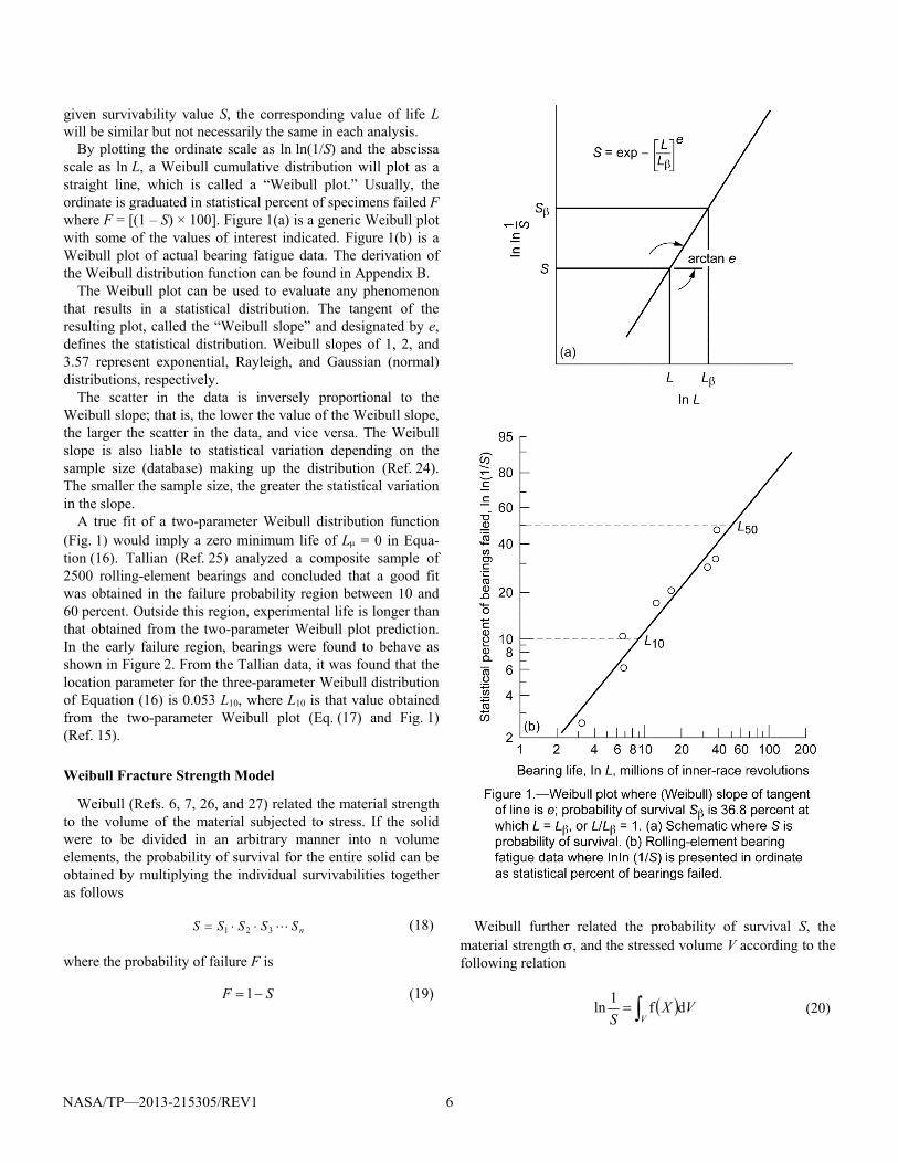
By plotting the ordinate scale as ln ln(1/S) and the abscissa scale as ln L, a Weibull cumulative distribution will plot as a straight line, which is called a “Weibull plot.” Usually, the ordinate is graduated in statistical percent of specimens failed F where F = [(1 – S) × 100]. Figure 1(a) is a generic Weibull plot with some of the values of interest indicated. Figure 1(b) is a Weibull plot of actual bearing fatigue data. The derivation of the Weibull distribution function can be found in Appendix B.

The Weibull plot can be used to evaluate any phenomenon that results in a statistical distribution. The tangent of the resulting plot, called the “Weibull slope” and designated by e, defines the statistical distribution. Weibull slopes of 1, 2, and 3.57 represent exponential, Rayleigh, and Gaussian (normal) distributions, respectively.

The scatter in the data is inversely proportional to the Weibull slope; that is, the lower the value of the Weibull slope, the larger the scatter in the data, and vice versa. The Weibull slope is also liable to statistical variation depending on the sample size (database) making up the distribution (Ref. 24). The smaller the sample size, the greater the statistical variation in the slope.

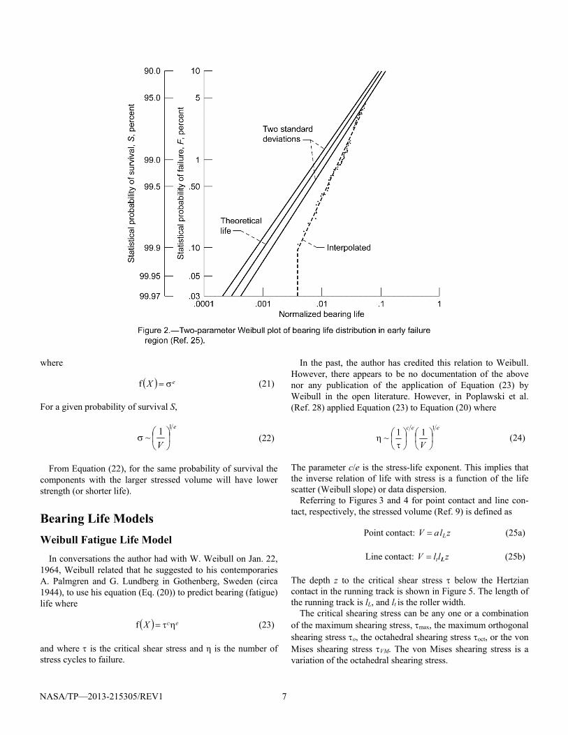
A true fit of a two-parameter Weibull distribution function (Fig. 1) would imply a zero minimum life of L = 0 in Equa-tion (16). Tallian (Ref. 25) analyzed a composite sample of 2500 rolling-element bearings and concluded that a good fit was obtained in the failure probability region between 10 and 60 percent. Outside this region, experimental life is longer than that obtained from the two-parameter Weibull plot prediction. In the early failure region, bearings were found to behave as shown in Figure 2. From the Tallian data, it was found that the location parameter for the three-parameter Weibull distribution of Equation (16) is 0.053 L10, where L10 is that value obtained from the two-parameter Weibull plot (Eq. (17) and Fig. 1) (Ref. 15).

Weibull Fracture Strength Model

Weibull (Refs. 6, 7, 26, and 27) related the material strength to the volume of the material subjected to stress. If the solid were to be divided in an arbitrary manner into n volume elements, the probability of survival for the entire solid can be obtained by multiplying the individual survivabilities together as follows

nSSSSS 321 (18)

where the probability of failure F is

SF 1 (19)

Weibull further related the probability of survival S, the

material strength , and the stressed volume V according to the following relation

VVX

Sdf

1ln (20)

NASA/TP—2013-215305/REV1 7

where

eX f (21)

For a given probability of survival S,

e

V

11

~

(22)

From Equation (22), for the same probability of survival the components with the larger stressed volume will have lower strength (or shorter life).

Bearing Life Models

Weibull Fatigue Life Model

In conversations the author had with W. Weibull on Jan. 22, 1964, Weibull related that he suggested to his contemporaries A. Palmgren and G. Lundberg in Gothenberg, Sweden (circa 1944), to use his equation (Eq. (20)) to predict bearing (fatigue) life where

ecX f (23)

and where is the critical shear stress and η is the number of stress cycles to failure.

In the past, the author has credited this relation to Weibull. However, there appears to be no documentation of the above nor any publication of the application of Equation (23) by Weibull in the open literature. However, in Poplawski et al. (Ref. 28) applied Equation (23) to Equation (20) where

eec

V

111

~

(24)

The parameter c/e is the stress-life exponent. This implies that the inverse relation of life with stress is a function of the life scatter (Weibull slope) or data dispersion.

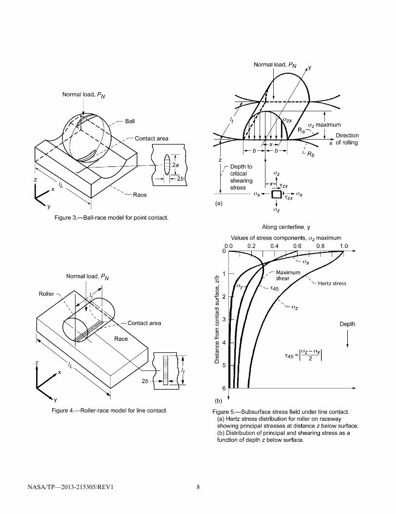
Referring to Figures 3 and 4 for point contact and line con-tact, respectively, the stressed volume (Ref. 9) is defined as

Point contact: zlaV L (25a)

Line contact: zllV t L (25b)

The depth z to the critical shear stress below the Hertzian contact in the running track is shown in Figure 5. The length of the running track is lL, and lt is the roller width.

The critical shearing stress can be any one or a combination of the maximum shearing stress, max, the maximum orthogonal shearing stress o, the octahedral shearing stress oct, or the von Mises shearing stress VM. The von Mises shearing stress is a variation of the octahedral shearing stress.

NASA/TP—2013-215305/REV1 8

NASA/TP—2013-215305/REV1 9

From Hertz theory (Refs. 11 and 29) for point contact (Fig. 3), V and can be expressed as a function of the maxi-mum Hertz (contact) stress, Smax (Ref. 29), where

max~ S (26a)

2max~ SV (26b)

Substituting Equations (26a) and (26b) in Equation (24) and L for η,

nSSS

L~ee

c

max2maxmax

1~

111

(27)

From Reference 28, solving for the value of the exponent n for point contact (ball in a raceway) from Equation (27) gives

e

cn

2 (28)

From Hertz theory for line contact (roller in a raceway, Fig. 4),

max~ SV (29)

Substituting Equations (26a) and (29) in Equation (24) and L for η,

nSSS

Lee

c

maxmaxmax

1~

11~

1

(30)

Solving for the value of n for line contact by substituting Equations (25a) and (28) into Equation (26) gives

e

cn

1 (31)

From Lundberg and Palmgren (Ref. 9) for point contact, c = 10.33 and e = 1.11. Then from Equation (28),

12.1111.1

233.102

e

cn (32)

From Hertz theory (Ref. 29) for point contact,

31~max PS (33)

From Equation (27) for point contact,

p

Nn PS

L1

~1

~max

(34a)

Combining Equations (33) and (34a) for point contact, and solving for p,

e

cnp

3

2

3

(34b)

From Equation (32) where n = 11.12,

7.33

12.11p (34c)

For line contact from Equation (31),

21.1011.1

133.101

e

cn (35)

From Equation (30) for line contact,

p

Nn P

~S

L~11

max

(36a)

From Hertz theory (Ref. 29) for line contact,

21~max PS (36b)

Combining Equations (36a) and (36b) and solving for p for line contact,

1.52

21.10

2

1

2

e

cnp (36c)

In their 1952 publication (Ref. 10), Lundberg and Palmgren assume e = 1.125 for line contact, then from Equation (35), n = 10.1, and from Equation (36c), p = 5. From Weibull, the values of the stress-life and the load-life exponents are depend-ent on the Weibull slope e, which for rolling-element bearings can and usually varies between 1 and 2. As a result, the values of the exponents can only be valid for a single value of the Weibull slope. As an example, if in Equation (32) for point contact, a Weibull slope e of 1.02 were selected, then n = 12 and p = 4 from Equation (34b). These values did not fit the bearing database that existed in the 1940s.

Lundberg-Palmgren Model

In 1947 Lundberg and Palmgren (Ref. 9) applied the Weibull analysis to the prediction of rolling-element bearing fatigue life. In order to better match the values of the Hertz stress-life exponent n and the load-life exponent p with experimentally determined values from pre-1940 tests on air-melt steel bearings, they introduced another variable, the depth to the critical shearing stress z to the h power where f (x) in Equa-tion (20) can be expressed as

NASA/TP—2013-215305/REV1 10

h

ec

zxf

(37)

The rationale for introducing zh was that it took a finite time period for a crack to initiate at a distance from the depth of the critical shearing to the rolling surface. Lundberg and Palmgren assumed that the time for crack propagation was a function of zh.

Equation (24) thus becomes

eh

eec

zV

1

11~

(38)

where is the life in stress cycles. For their critical shearing stress, Lundberg and Palmgren

chose the orthogonal shearing stress. From Hertz theory (Ref. 29),

max~ Sz (39)

For point contact, substituting Equations (26a), (26b), and (39) in Equation (38) and L for η,

nS

SSS

L eh

eec

maxmax2

maxmax

1~

11~

1

(40)

From Reference 28, solving for the value of the exponent n for point contact (ball on a raceway) from Equation (40) gives

e

hcn

2 (41a)

From Lundberg and Palmgren (Ref. 9), using values of 1.11 for e, c = 10.33, and h = 2.33, from Equation (41a) for point contact

911.1

33.2233.10

n (41b)

From Equation (34b) for point contact, where n = 9,

33

9

3

np (41c)

For line contact, substituting Equations (26a), (29), and (39) in Equation (38) and L for η,

nSSSS

Le

hee

c

maxmaxmaxmax

1~

111~

1

(42)

From Equation (42) solving for n for line contact,

e

hcn

1 (43a)

Using previous values of c and h, and e = 1.125 for line contact,

8125.1

33.2133.10

n (43b)

From Equation (36b) for line contact,

42

8

2

np (43c)

These values of n and p for point and line contacts correlated to the then-existing rolling-element bearing database.

In their 1952 paper (Ref. 10), Lundberg and Palmgren modi-fied their value of the load-life exponent p for roller bearings from 4 to 10/3. The rationale for doing so was that various roller bearing types had one contact that is line contact and other that is point contact. They state, “…as a rule the contacts between the rollers and the raceways transforms from a point to a line contact for some certain load so that the life exponent varies from 3 to 4 for differing loading intervals within the same bearing.” The ANSI/ABMA and ISO standards (Refs. 12 and 14) incorporate p = 10/3 for roller bearings. Computer codes for rolling-element bearings incorporate p = 4.

Strict Series Reliability

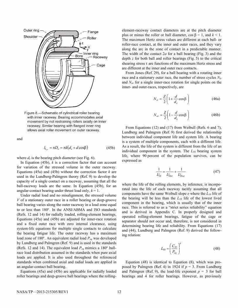
Figures 6 and 7 show schematics of deep-groove and angular-contact ball bearings. Figure 8 is a schematic of a roller bearing. From Equations (20) and (30), the fatigue life L of a bearing inner or outer race determined from the Lundberg-Palmgren theory (Ref. 9) can be expressed as follows:

eh

eec

zNV

AL

111

1

(44)

where N is the number of stress cycles per inner-race revolution and A is a material life factor based upon air-melt, pre-1940 AISI 52100 steel3 and mineral oil lubricant.

In general, for ball and roller bearings, the running track lengths for Equations (25a) and (25b) for the inner and outer raceways are, respectively,

cosddDl eiLir (45a)

3 Numbered AISI steel grades are standardized by the American Iron and Steel Institute (AISI).

NASA/TP—2013-215305/REV1 11

NASA/TP—2013-215305/REV1 12

and

cosddkDl eoLor (45b)

where de is the bearing pitch diameter (see Fig. 6). In Equation (45b), k is a correction factor that can account

for variation of the stressed volume in the outer raceway. Equations (45a) and (45b) without the correction factor k are used in the Lundberg-Palmgren theory (Ref. 9) to develop the capacity of a single contact on a raceway, assuming that all the ball-raceway loads are the same. In Equation (45b), for an angular-contact bearing under thrust load only, k = 1.

Under radial load and no misalignment, the stressed volume V of a stationary outer race in a roller bearing or deep-groove ball bearing varies along the outer raceway in a load zone equal to or less than 180. In the ANSI/ABMA and ISO standards (Refs. 12 and 14) for radially loaded, rolling-element bearings, Equations (45a) and (45b) are adjusted for inner-race rotation and a fixed outer race with zero internal clearance, using system-life equations for multiple single contacts to calculate the bearing fatigue life. The outer raceway has a maximum load zone of 180. An equivalent radial load Peq was developed by Lundberg and Palmgren (Ref. 9) and is used in the standards (Refs. 12 and 14). The equivalent load Peq mimics a 180 ball-race load distribution assumed in the standards when pure axial loads are applied. It is also used throughout the referenced standards when combined axial and radial loads are applied in an angular-contact ball bearing.

Equations (45a) and (45b) are applicable for radially loaded roller bearings and deep-groove ball bearings where the rolling-

element-raceway contact diameters are at the pitch diameter plus or minus the roller or ball diameter, cos β = 1, and k < 1. The maximum Hertz stress values are different at each ball- or roller-race contact, at the inner and outer races, and they vary along the arc in the zone of contact in a predictable manner. The width of the contact 2a for a ball bearing (Fig. 3) and the depth z for both ball and roller bearings (Fig. 5) to the critical shearing stress are functions of the maximum Hertz stress and are different at the inner and outer race contacts.

From Jones (Ref. 29), for a ball bearing with a rotating inner race and a stationary outer race, the number of stress cycles Nir and Nor for a single inner-race rotation for single points on the inner- and outer-races, respectively, are

cos1

2 eir

d

dZN (46a)

cos1

2 eor

d

dZN (46b)

From Equations (12) and (17) from Weibull (Refs. 6 and 7), Lundberg and Palmgren (Ref. 9) first derived the relationship between individual component life and system life. A bearing is a system of multiple components, each with a different life. As a result, the life of the system is different from the life of an individual component in the system. The L10 bearing system life, where 90 percent of the population survives, can be expressed as

e

ore

ire LLL 101010

111 (47)

where the life of the rolling elements, by inference, is incorpo-rated into the life of each raceway tacitly assuming that all components have the same Weibull slope e where the L10 life of the bearing will be less than the L10 life of the lowest lived component in the bearing, which is usually that of the inner race. This is referred to as a “strict series reliability” equation and is derived in Appendix C. In properly designed and operated rolling-element bearings, fatigue of the cage or separator should not occur and, therefore, is not considered in determining bearing life and reliability. From Equations (17) and (44), Lundberg and Palmgren (Ref. 9) derived the follow-ing relation:

p

eq

D

P

CL

10 (48)

Equation (48) is identical to Equation (8), which was pro-posed by Palmgren (Ref. 4) in 1924 if p = 3. From Lundberg and Palmgren (Ref. 9), the load-life exponent p = 3 for ball bearings and 4 for roller bearings. However, as previously

NASA/TP—2013-215305/REV1 13

discussed, Lundberg and Palmgren in 1952 (Ref. 10) proposed p = 10/3 for roller bearings.

Dynamic Load Capacity, CD

Palmgren (Ref. 4) proposed the concept of a dynamic load rating or capacity for a rolling-element bearing, defined as the load placed on a bearing that will theoretically result in a L10 life of 1 million inner-race revolutions. He first characterized this concept as that shown in Equation (6) that subsequently evolved as Equations (9) and (10).

From Anderson (Ref. 21), according to the Hertz theory the dynamic load capacity should be proportional to the square of the rolling-element diameter. From experimental data, Palmgren (Ref. 30) found that capacity varied as d1.8 for balls up to about 25 mm in diameter and d1.4 for balls larger than 25 mm in diameter.

From Equation (11), the dynamic load capacity varies with the number of rolling elements Z to the 2/3 power (Z2/3). However, this would only be correct for an inverse cubic relation between load and life.

From Anderson (Ref. 21), multiple-row bearings with i rows of balls may be considered as a combination of i single-row bearings. From strict series reliability (Appendix C) the following relation between the life of a multirow bearing and the lives of the i individual rows is obtained assuming all rows carry equal load:

ei

eee LLLL

1111

21

(49a)

Then

ei

e L

i

L

1 (49b)

If each row of the bearing is loaded with a load equal to the dynamic load capacity of one row Ci, then Li = 1 (i.e., one million inner-race revolutions) and from Equation (49b),

i

Le 1 (50a)

or

ei

L1

1 (50b)

The load Peq on the entire bearing is iCi, where Peq is the equivalent bearing load:

ieq iCP (51)

From Equations (50b) and (51),

e

n

i

D

iiC

C1

1

(52a)

or

epiD iCC 11 (52b)

For ball bearings, p = 3 and e is approximately 1.1, so that the capacity of multirow bearings varies as i0.7. For radial ball bear-ings, the normal force between a ball and a race varies as 1/cos β, so that the capacity is proportional to cos β, where β is the contact angle (see Fig. 7). The influence of the ball-race conformity, bearing type, and internal dimensions expressed by fcm/(cos β)0.3, where fcm is the material and geometry coefficient. Therefore the capacity of a radial ball bearing varies as (icos β)0.7.

For thrust ball bearings, the normal force between a ball and a race varies as 1/sin β, so that the capacity is proportional to sin β or to (cos β)(tan β). When the influences of the degree of conformity, of bearing type, and of internal dimensions are included, the capacity of a thrust ball bearing varies as (icos β) 0.7(tan β).

For roller bearings with line contact, the load-life exponent in the life equation is 4, so that the capacity varies as Z3/4. From Equation (52b) with p = 4, the capacity of a multirow-roller bearing is found to vary as i0.78. Theoretically, the capacity of roller bearings should be proportional to ltd. Experimental data (Ref. 9) indicate that capacity varies as 07.178.0 dlt .

Formulas for the dynamic load capacity CD as developed by Palmgren (Ref. 30) and Lundberg and Palmgren (Refs. 9 and 10) are dependent on

(1) Size of rolling elements, d (ball or roller diameter) and lt (roller length)

(2) Number of rolling elements per row, Z (3) Number of rows of rolling elements, i (4) Contact angle, (see Fig. 7) (5) Material and geometry coefficient, fcm

(6) Units factor, u = 3.647 for metric units (Newtons and millimeters) or 1.00 for English units (pounds force and inches) for ball bearings for d > 25.4 mm

The dynamic load capacity below for radially loaded bearings is designated as CDr, and for axial loaded bearings it is CDa. The units factor u is used to avoid a discontinuity in CD at d = 25.4 mm for ball bearings.

The formulas are semiempirical and are incorporated into the ANSI/ABMA and ISO standards (Refs. 12 to 14). They are as follows:

(1) Ball bearings a. For radial ball bearings with d 25.4 mm,

8.17.03

2cos dZifC cmrD , N (lb) (53a)

NASA/TP—2013-215305/REV1 14

b. For radial ball bearings with d 25.4 mm,

4.17.03

2cos dZiufC cmrD , N (lb) (53b)

c. For thrust ball bearings with 90° and d 25.4 mm,

8.13/27.0 tancos dZifC cmDa , N (lb) (53c)

d. For thrust ball bearings with 90° and d ˃ 25.4 mm,

4.13/27.0 tancos dZiufC cmDa , N (lb) (53d)

e. For thrust ball bearings with = 90° and d 25.4 mm,

8.13/27.0 dZifC cmDa , N (lb) (53e)

f. For thrust ball bearings with = 90° and d ˃ 25.4 mm,

4.13/27.0 dZiufC cmDa , N (lb) (53f)

(2) Roller bearings a. For radial roller bearings,

2729

439

7

cos dZlifC tcmrD , N (lb) (53g)

b. For thrust roller bearings with 90°,

27/294/39/7 tancos dZlifC tcmDa , N (lb) (53h)

c. For thrust roller bearings with = 90°,

27/294/39/7 dZlifC tcmDa , N (lb) (53i)

The material and geometry coefficient fcm (originally desig-nated fc by Lundberg and Palmgren (Ref. 9)) in turn depends on the bearing type, material, and processing and the conformity between the rolling elements and the races. Representative values of fcm are given in Table I from the ANSI/ABMA standards (Refs. 13 and 14). It should be noted that the coeffi-cient fcm and the various exponents of Equations (53a) through (53g) were chosen by Lundberg and Palmgren (Ref. 9) and Palmgren (Ref. 30) to match their bearing database at the time of their writing. However, the values of fcm have been updated periodically in the ANSI/ABMA and ISO standards (Table II) (Refs. 18 and 31). The standards and the bearing manufactur-ers’ catalogs generally normalize their values of fcm to conform-ities on the inner and outer races of 0.52 (52 percent) (Ref. 31).

Substituting the bearing geometry and the Hertzian contact stresses for a given normal load PN into Equations (44) through (47), the dynamic load capacity CD can be calculated from Equation (48). Since PN is the normal load on the maximum-loaded rolling element, it is required that the equivalent load Peq

TABLE I.—REPRESENTATIVE VALUES OF ROLLING-ELEMENT BEARING GEOMETRY AND MATERIAL COEFFICIENT fcm IN ANSI/ABMA STANDARDSa 9 AND 11 FOR REPRESENTATIVE

ROLLING-ELEMENT BEARING SIZES [From Ref. 18.]

Bearing envelope size,c

d cos de

Bearing geometry and material coefficient,a fcm

b Deep-groove and angular-

contact ball bearingsc Cylindrical (radial)

roller bearing

0.05 60.71 (4614)

81.51 (7324)

.10 72.15 (5483)

92.62 (8322)

.16 77.58 (5888)

97.35 (8747)

.22 77.48 (5888)

97.02 (8718)

.28 74.23 (5640)

93.72 (8767)

.34 69.16 (5256)

-------

.40 62.92 (4782)

-------

aStandards 9 and 11 are found in Refs. 13 and 14, respectively. bValues of fcm are for use with newtons and millimeters; those in parentheses are for use with pounds and inches.

cPrior to 1990, fcm was designated as fc. dd is rolling element diameter, is contact angle, and de is pitch diameter. eInner- and outer-race conformities are equal to 0.52.

TABLE II.—REPRESENTATIVE VALUES OF ROLLING-ELEMENT BEARING GEOMETRY AND MATERIAL COEFFICIENT fcm IN ANSI/ABMA STANDARD 9 (REF. 13) FOR REPRESENTATIVE

BALL BEARING SIZES BY YEAR INTRODUCED (REF. 31) [Inner- and outer-race conformities are equal to 0.52.]

Bearing size,a

d cos de

Bearing geometry and material coefficient,b fcm

c 1960 1972 1978 1990

0.05 46.75 (3550)

59.52 (4520)

46.75 (3550)

60.70 (4610)

.10 55.57 (4220)

73.34 (5570)

55.57 (4220)

72.16 (5480)

.16 59.65 (4530)

84.41 (6410)

59.65 (4530)

77.56 (5890)

.22 59.65 (4530)

92.96 (7060)

59.65 (4350)

77.56 (5890)

.28 57.15 (4340)

100.08 (7600)

57.15 (4340)

74.27 (5640)

.34 53.33 (4050)

106 (8050)

53.33 (4050)

69.26 (5260)

.40 ------ ------- 75.94 (3670)

62.94 (4780)

ad = ball diameter, mm (in.); de = pitch diameter, mm (in.); and = free contact angle, degrees.

bValues of fcm are for use with newtons and millimeters; those in parentheses are for use with pounds and inches.

cPrior to 1990, fcm was designated as fc.

be calculated. Once CD is determined, fcm can be calculated for the appropriate bearing type from Equation (53).

NASA/TP—2013-215305/REV1 15

The equivalent load Peq can be obtained from Equation (3) where values of X and Y for different bearing types are given in the ANSI/ABMA standards (Refs. 13 and 14). The dynamic load capacity CD in the standards should be CDr (Eqs. (53a), (53b), and (53g)) for a radial bearing or CDa (Eqs. (53c) to (53f), (53h), and (53i)) for a thrust bearing.

Lives determined using Equation (53) are based on the “first evidence of fatigue.” This can be a small spall or surface pit that may not significantly impair the function of the bearing. The actual useful bearing life can be much longer. It should be also noted that in these Equations (53) where derived expo-nents differed from those obtained experimentally, those exponents obtained experimentally were substituted by Lundberg and Palmgren (Refs. 9 and 10) for those that they analytically derived.

Ioannides-Harris Model

Ioannides and Harris (Ref. 32), using Weibull (Refs. 6 and 7) and Lundberg and Palmgren (Refs. 9 and 10), introduced a fatigue-limiting shear stress u (App. A) where from Equation (37),

h

ecu

zXf

(54)

The equation is identical to that of Lundberg and Palmgren (Eq. (37)) except for the introduction of a fatigue-limiting stress where

eh

eec

zVu

1

11~

(55)

Equation (55) can be expressed as a function of Smax where

u

eh

eec

nu S

zV

L

max

1~

11~

1

(56)

Ioannides and Harris (Ref. 32) use the same values of Lundberg and Palmgren for e, c, and h. If u equals 0, then the values of the Hertz stress-life exponent n are identical to those of Lundberg and Palmgren (Eqs. (41b) and (43b)). However, for values of u 0, n is also a function of ( – u). For their critical shearing stress, Ioannides and Harris chose the von Mises stress.

From the above, Equation (48) can be rewritten to include a “fatigue-limiting” load Pu:

p

ueq

D

PP

CL

10 (57a)

where

uu fP (57b)

When Peq Pu, bearing life is infinite and no failure would be expected. When Pu = 0, the life is the same as that for Lundberg and Palmgren.

The concept of a fatigue limit for rolling-element bearings was first proposed by Palmgren in 1924 (Eq. (5)) (Ref. 4). It was apparently abandoned by him first in 1936 (Ref. 33) and then again with Lundberg in 1947 (Ref. 9). In 1936 Palmgren published the following:

“For a few decades after the manufacture of ball bear-ings had taken up on modern lines, it was generally con-sidered that ball bearings, like other machine units, were subject to a fatigue limit; that is, that there was a limit to their carrying capacity beyond which fatigue speedily sets in, but below which the bearings could continue to function for infinity. Systematic examination of the results of tests made in the SKF laboratories before 1918, however, showed that no fatigue limit existed within the range covered by the comparatively heavy loads employed for test purposes. It was found that so far as the scope of the investigation was concerned, the employment of a lighter load invariably had the effect of increasing the number of revolutions a bearing could execute before fatigue set in. It was certainly still assumed that a fatigue limit coexisted with a low specific load, but tests with light loads finally showed that the fatigue limit for infinite life, if such exists, is reached under a lighter load than all of those employed, and that in practice the life is accordingly always a function of load.”

In 1985, Ioannides and Harris (Ref. 32) applied Palmgren’s 1924 (Ref. 4) concept of a fatigue limit to the 1947 Lundberg-Palmgren equations (Ref. 9) in the form shown in Equation (54). The ostensible reason Ioannides and Harris used the fatigue limit was to replace the material and processing life factors (Ref. 18) that are used as life modifiers in conjunction with the bearing lives calculated from the Lundberg-Palmgren equations.

There are two problems associated with the use of a fatigue limit for rolling-element bearing. The first problem is that the form of Equation (55) may not reflect the presence of a fatigue limit but the presence of a compressive residual stress (Refs. 18 and 28). The second problem is that there are no data in the open literature that would justify the use of a fatigue limit for through-hardened bearing steels such as AISI 52100 and AISI M–50.

In 2007, Sakai (Ref. 34) discussed experimental results obtained by the Research Group for Material Strength in Japan. He presented stress-life rotating bending fatigue life data from six different laboratories in Japan for AISI 52100 bearing steel. He presented stress-life fatigue data for axial loading. The

NASA/TP—2013-215305/REV1 16

resultant lives were in excess of a billion (109) stress cycles at maximum shearing stresses (max) as low as 0.35 GPa (50.8 ksi) without an apparent fatigue limit.

In 2008, Tosha et al. (Ref. 35) reported the results of rotating beam fatigue experiments for through-hardened AISI 52100 bearing steel at very low shearing stresses as low as 48 GPa (69.6 ksi). “The results produced fatigue lives in excess of 100 million stress cycles without the manifestation of a fatigue limit.”

In order to assure the credibility of their work, additional re-search was conducted and published by Shimizu, et al. (Ref. 36). They tested six groups of AISI 52100 bearing steel specimens using four-alternating torsion fatigue life test rigs to determine whether a fatigue limit exists or not and to compare the resultant shear stress-life relaxation with that used for rolling-element bearing life prediction. The number of specimens in each sample size ranged from 19 to 33 specimens for a total of 150 tests. The tests were run at 0.50, 0.63, 0.76, 0.80, 0.95, and 1.00 GPa (75.5, 91.4, 110.2, 116.0, 137.8, and 145.0 ksi) maximum shearing stress amplitudes. The stress-life curves of these data show an inverse dependence of life on shearing stress, but do not show an inverse relation for inverse dependence of the shearing stress minus a fatigue limiting stress. The shear stress-life exponent for the AISI 52100 steel was 10.34 from a three-parameter Weibull analysis and was independent of the Weibull slope e.

Recent publications by the American Society of Mechanical Engineers (ASME) (Ref. 37) and the ISO (Refs. 38 and 39) for calculating the life of rolling-element bearings include a fatigue limit and the effects of ball-race conformity on bearing fatigue life. These methods do not, however, include the effect of ball failure on bearing life. The ISO method is based on the work reported by Ioannides, Bergling, and Gabelli (Ref. 40). The ASME method as contained in their ASMELIFE software (Ref. 37) uses the von Mises stress as the critical shearing stress with a fatigue limit value of 684 MPa (99 180 psi). This corresponds to a Hertz surface contact stress of 1140 MPa (165 300 psi). The ISO 281:2007 method (Ref. 39) uses a fatigue limit stress of 900 MPa (130 500 psi), which corresponds to a Hertz contact stress of 1500 MPa (217 500 psi) (Ref. 31).

The concepts of a fatigue limit load (bearing load under which the fatigue stress limit is just reached in the most heavily loaded raceway contact) introduced in the new ISO rating methods (Ref. 39) is proportional to the fatigue limit load raised to the 3rd power for ball bearings (point contact). By using ISO 281:2007 (Ref. 39), these differing values of load would result in a 128-percent higher load below which no fatigue failure would be expected to occur (Ref. 31) than by using ASMELIFE (Ref. 37).

The effect of using different values of fatigue limit or no fatigue limit on rolling-element fatigue life prediction is shown in Table III. This table summarizes the qualitative results obtained for maximum Hertz stresses of 1379, 1724, and 2068 MPa (200, 250, and 300 ksi) for point contact using Equation (38) for Lundberg-Palmgren without a fatigue limit

TABLE III.—EFFECT OF FATIGUE LIMIT τ ON ROLLING-ELEMENT FATIGUE LIFE

[From Ref. 31.] Fatigue limit,a

u, MPa (ksi)

Relative lifeb,c (Eq. (58))

Maximum Hertz stress, MPa (ksi)

1379 (200)

1724 (250)

2068 (300)

0 (0), Lundberg-Palmgren (Ref. 9) 1 0.134 0.026 684 (99.2), ASMELIFE (Ref. 37) 11.9106 3152 44.6

900 (130.5), ISO 281:2007 (Ref. 39) ∞ 23.3106 4258 aThe von Mises stress. bIncludes effect of stressed volume. cNormalized to life at maximum Hertz stress of 1379 MPa (200 ksi) with no fatigue limit.

and Equation (55) for fatigue limits of 684 MPa (99 180 psi) (from ASMELIFE) and 900 MPa (130 500 psi) (from ISO 281:2007). The results are normalized to a maximum Hertz stress of 1379 MPa (200 ksi) with no fatigue limit where the quotient of Equation (55) divided by Equation (38) is taken to the c/e power of 9.3 (taken from Lundberg and Palmgren). The effect of stressed volume was also factored into these calcula-tions (Ref. 31):

e

c

uIH LL

(58)

where LIH is the life with the fatigue limit u, L is the life without a fatigue limit u, and is the critical shearing stress.

Zaretsky Model

Both the Weibull and Lundberg-Palmgren models relate the critical shear stress-life exponent c to the Weibull slope e. The parameter c/e thus becomes, in essence, the effective critical shear stress-life exponent, implying that the critical shear stress-life exponent depends on bearing life scatter or disper-sion of the data. A search of the literature for a wide variety of materials and for nonrolling-element fatigue reveals that most stress-life exponents vary from 6 to 12. The exponent appears to be independent of scatter or dispersion in the data. Hence, Zaretsky (Ref. 41) has rewritten the Weibull equation to reflect that observation by making the exponent c independent of the Weibull slope e, where

eceXf (59)

From Equations (5) and (59), the life in stress cycles is given by

e

V

c 1

11~

(60)

NASA/TP—2013-215305/REV1 17

For critical shearing stress , Zaretsky chose the maximum shearing stress, 45.

Lundberg and Palmgren (Ref. 9) assumed that once initiated, the time a crack takes to propagate to the surface and form a fatigue spall is a function of the depth to the critical shear stress z. Hence, by implication, bearing fatigue life is crack propaga-tion time dependent. However, rolling-element fatigue life can be categorized as “high-cycle fatigue.” Crack propagation time is an extremely small fraction of the total life or running time of the bearing. The Lundberg-Palmgren relation implies that the opposite is true. To decouple the dependence of bearing life on crack propagation rate, Zaretsky (Refs. 41 and 42) dis-pensed with the Lundberg-Palmgren relation of L ~ zh/e in Equation (60). (It should be noted that at the time (1947) Lundberg and Palmgren published their theory, the concepts of “high-cycle” and “low-cycle” fatigue were only then beginning to be formulated.)

Equation (60) can be written as

n

ec

SVL

max

/11

~11

~

(61)

From Reference 28, solving for the value of the Hertz stress-life exponent n, for point contact from Equation (61) gives

e

cn2

(62a)

and for line contact,

e

cn1

(62b)

If it is assumed that c = 9 and e = 1.11, n = 10.8 for point contact and n = 9.9 for line contact. If it is further assumed that c = 10 and e = 1.0, n = 12 for point contact and n = 11 for line contact.

What differentiates Equation (61) from those of Weibull (Eq. 24), Lundberg and Palmgren (Eq. (38)) and Ioannides and Harris (Eq. (56)) is that the relation between shearing stress and life is independent of the Weibull slope, e, or the distribution of the failure data. However, in all four models, there is a depend-ency of the Hertz stress-life exponent, n, on the Weibull slope. The magnitude of the variation is least with the Zaretsky model.

Although Zaretsky (Refs. 41 and 42) does not propose a fatigue-limiting stress, he does not exclude that concept either. However, his approach is entirely different from that of Ioannides and Harris (Ref. 32). For critical stresses less than the fatigue-limiting stress, the life for the elemental stressed volume is assumed to be infinite. Thus, the stressed volume of the component would be affected where L ~ 1/V

l/e. As an example, a reduction in stressed volume of 50 percent results in an increase in life by a factor of 1.9.

Ball and Roller Set Life

Lundberg and Palmgren (Ref. 9) do not directly calculate the life of the rolling-element (ball or roller) set of the bearing. However, through benchmarking of the equations with bearing life data by use of a material-geometry factor fcm, the life of the rolling-element set is implicitly included in the life calculation of Equations (53a) to (53g).

The rationale for not including the rolling-element set in Equation (47) appears in the 1945 edition of A. Palmgren’s book (Ref. 5) wherein he states, “…the fatigue phenomenon which determines the life (of the bearing) usually develops on the raceway of one ring or the other. Thus, the rolling elements are not the weakest parts of the bearing….” The database that Palmgren used to benchmark his and later the Lundberg-Palmgren equations were obtained under radially loaded conditions. Under these conditions, the life of the rolling elements as a system (set) will be equal to or greater than that of the outer race. As a result, failure of the rolling elements in determining bearing life was not initially considered by Palmgren. Had it been, Equation (47) would have been written as follows (with L correlating to the recalculated lives):

e

or

e

re

e

ir

e

LLLL

1111

10

(63)

where irir LL , oror LL , and iroriror LLLL and where

the Weibull slope e will be the same for each of the compo-nents as well as for the bearing as a system, provided all components are of the same material.

Comparing Equation (63) with Equation (47), the value of the L10 bearing life will be the same. However, the values of the Lir and Lor as well as irL and orL between the two equations

will not be the same, but the ratio of Lor/Lir and iror LL will

remain unchanged. The fraction of failures due to the failure of a bearing com-

ponent is expressed by Johnson (Ref. 24) as

Fraction of inner-race failures e

irL

L

10 (64a)

Fraction of rolling-element failures e

reL

L

10 (64b)

Fraction of outer-race failures e

orL

L

10 (64c)

From Equations (64a) to (64c), if the life of the bearing and the fractions of the total failures represented by the inner race, the outer race, and the rolling element set are known, the life of

NASA/TP—2013-215305/REV1 18

each of these components can be calculated. Hence, by obser-vation, it is possible to determine the life of each of the bearing components with respect to the life of the bearing.

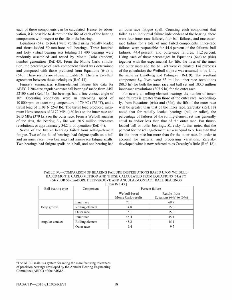
Equations (64a) to (64c) were verified using radially loaded and thrust-loaded 50-mm-bore ball bearings. Three hundred and forty virtual bearing sets totaling 31 400 bearings were randomly assembled and tested by Monte Carlo (random) number generation (Ref. 43). From the Monte Carlo simula-tion, the percentage of each component failed was determined and compared with those predicted from Equations (64a) to (64c). These results are shown in Table IV. There is excellent agreement between these techniques (Ref. 43).

Figure 9 summarizes rolling-element fatigue life data for ABEC 7 204-size angular-contact ball bearings4 made from AISI 52100 steel (Ref. 44). The bearings had a free contact angle of 10°. Operating conditions were an inner-ring speed of 10 000 rpm, an outer-ring temperature of 79 °C (175 °F), and a thrust load of 1108 N (249 lb). The thrust load produced maxi-mum Hertz stresses of 3172 MPa (460 ksi) on the inner race and 2613 MPa (379 ksi) on the outer race. From a Weibull analysis of the data, the bearing L10 life was 20.5 million inner-race revolutions, or approximately 34.2 hr of operation (Ref. 44).

Seven of the twelve bearings failed from rolling-element fatigue. Two of the failed bearings had fatigue spalls on a ball and an inner race. Two bearings had inner-race fatigue spalls. Two bearings had fatigue spalls on a ball, and one bearing had

4The ABEC scale is a system for rating the manufacturing tolerances of precision bearings developed by the Annular Bearing Engineering Committee (ABEC) of the ABMA.

an outer-race fatigue spall. Counting each component that failed as an individual failure independent of the bearing, there were four inner-race failures, four ball failures, and one outer-race failure for a total of nine failed components. Inner-race failures were responsible for 44.4 percent of the failures; ball failures, 44.4 percent; and outer-race failures, 11.2 percent. Using each of these percentages in Equations (64a) to (64c) together with the experimental L10 life, the lives of the inner and outer races and the ball set were calculated. For purposes of the calculation the Weibull slope e was assumed to be 1.11, the same as Lundberg and Palmgren (Ref. 9). The resultant component L10 lives were 53 million inner-race revolutions (88.3 hr) for both the inner race and ball set and 183.3 million inner-race revolutions (305.5 hr) for the outer race.

For nearly all rolling-element bearings the number of inner-race failures is greater than those of the outer race. According-ly, from Equations (64a) and (64c), the life of the outer race will be greater than that of the inner race. Zaretsky (Ref. 18) noted that for radially loaded bearings (ball or roller), the percentage of failures of the rolling-element set was generally equal to and/or less than that of the outer race. For thrust-loaded ball or roller bearings, Zaretsky further noted that the percent for the rolling-element set was equal to or less than that for the inner race but more than for the outer race. In order to account for material and processing variations, Zaretsky developed what is now referred to as Zaretsky’s Rule (Ref. 18):

TABLE IV.—COMPARISON OF BEARING FAILURE DISTRIBUTIONS BASED UPON WEIBULL-BASED MONTE CARLO METHOD AND THOSE CALCULATED FROM EQUATIONS (64a) TO

(64c) FOR 50-mm-BORE DEEP-GROOVE AND ANGULAR-CONTACT BALL BEARINGS [From Ref. 43.]

Ball bearing type Component Percent failure

Weibull-based Monte Carlo results

Results from Equations (64a) to (64c)

Deep groove

Inner race 70.1 69.9

Rolling element 14.8 15.0

Outer race 15.1 15.0

Angular contact

Inner race 45.4 45.1

Rolling element 45.2 45.1

Outer race 9.4 9.7

NASA/TP—2013-215305/REV1 19

For radially loaded ball and roller bearings, the life of the

rolling–element set is equal to or greater than the life of the outer race. Let the life of the rolling-element set (as a system) be equal to that of the outer race.

From Equation (63) where reL = orL ,

e

or

e

ir

e

LLL

12

11

10

(65)

For thrust-loaded ball and roller bearings, the life of the rolling-element set is equal to or greater than the life of the inner race but less than that of the outer race. Let the life of the rolling-element set (as a system) be equal to that of the inner race.

From Equation (63) where reL = irL ,

e

or

e

ir

e

LLL

112

1

10

(66)

Examples of using Equations (65) and (66) are given in Reference 18. As previously stated, the resulting values for Lir

and Lor from these equations are not the same as those from Equation (47). They will be higher.

H. Takata (Ref. 45), using a modified approach to the Lundberg-Palmgren theory (Ref. 9), derived the basic dynamic load capacity of the rolling-element bearing set in addition to those for the inner and outer races for radial and thrust-loaded ball and roller bearings. For radially loaded ball bearings, Takata assumes random ball rotation. For thrust-loaded ball bearings, he assumes a single or fixed running track on each ball. According to Takata, the basic dynamic load capacity CD of a bearing system can be expressed as

1/ww w wD re orirC C C C

(67)

where CD is calculated from Equations (53a) and (53b) (from Lundberg-Palmgren, Ref. 9), and the exponent w is equal to 10/3 for ball bearings. Takata (Ref. 45) provides equations for calculating the dynamic load capacity of the rolling-element (ball) set, Cre. The resulting values for Cir and Cor will be higher than those from the Lundberg-Palmgren equations.

Takata (Ref. 45) performed a single ball-set life calculation within his paper for a 30-mm-bore deep-groove ball bearing. From this calculation he concluded that for this bearing

Cir < Cre < Cor (68a)

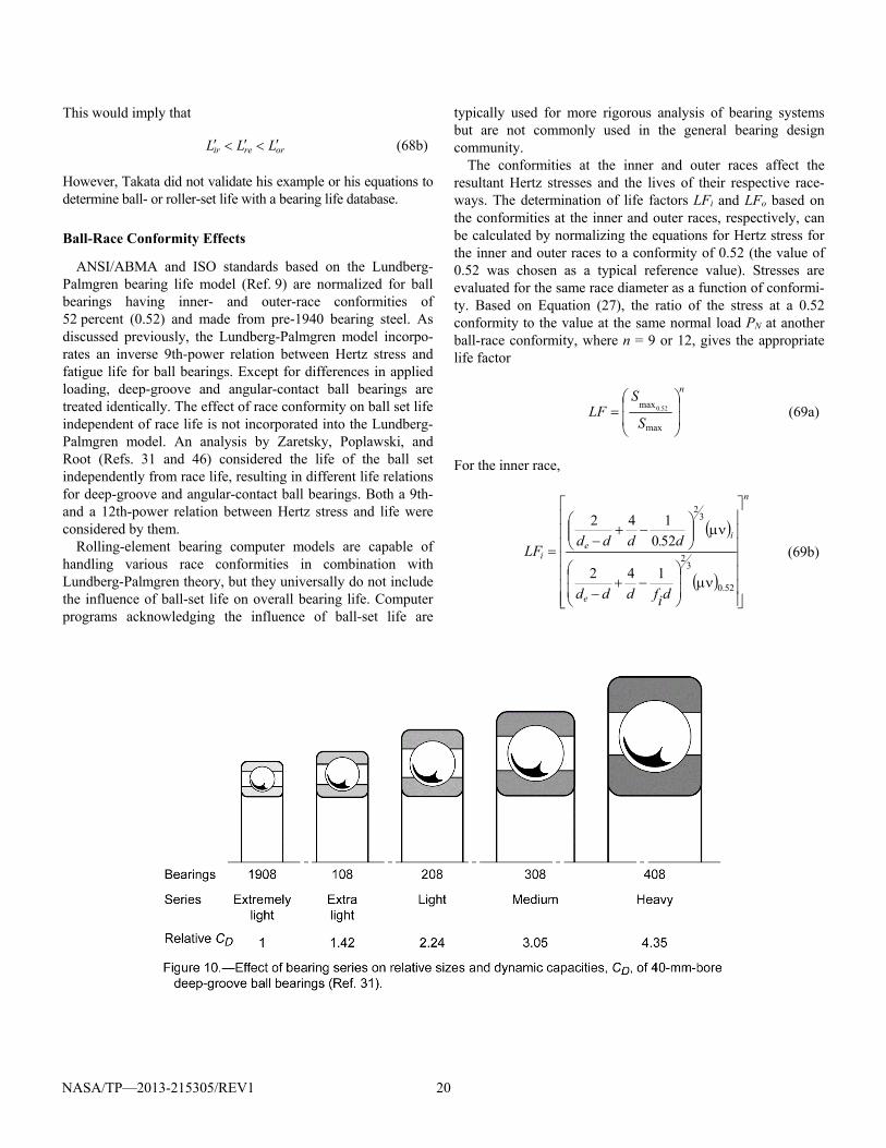
NASA/TP—2013-215305/REV1 20

This would imply that

orreir LLL (68b)

However, Takata did not validate his example or his equations to determine ball- or roller-set life with a bearing life database.

Ball-Race Conformity Effects

ANSI/ABMA and ISO standards based on the Lundberg-Palmgren bearing life model (Ref. 9) are normalized for ball bearings having inner- and outer-race conformities of 52 percent (0.52) and made from pre-1940 bearing steel. As discussed previously, the Lundberg-Palmgren model incorpo-rates an inverse 9th-power relation between Hertz stress and fatigue life for ball bearings. Except for differences in applied loading, deep-groove and angular-contact ball bearings are treated identically. The effect of race conformity on ball set life independent of race life is not incorporated into the Lundberg-Palmgren model. An analysis by Zaretsky, Poplawski, and Root (Refs. 31 and 46) considered the life of the ball set independently from race life, resulting in different life relations for deep-groove and angular-contact ball bearings. Both a 9th- and a 12th-power relation between Hertz stress and life were considered by them.

Rolling-element bearing computer models are capable of handling various race conformities in combination with Lundberg-Palmgren theory, but they universally do not include the influence of ball-set life on overall bearing life. Computer programs acknowledging the influence of ball-set life are

typically used for more rigorous analysis of bearing systems but are not commonly used in the general bearing design community.

The conformities at the inner and outer races affect the resultant Hertz stresses and the lives of their respective race-ways. The determination of life factors LFi and LFo based on the conformities at the inner and outer races, respectively, can be calculated by normalizing the equations for Hertz stress for the inner and outer races to a conformity of 0.52 (the value of 0.52 was chosen as a typical reference value). Stresses are evaluated for the same race diameter as a function of conformi-ty. Based on Equation (27), the ratio of the stress at a 0.52 conformity to the value at the same normal load PN at another ball-race conformity, where n = 9 or 12, gives the appropriate life factor

n

S

SLF

max

max 52.0 (69a)

For the inner race,

n

e

ie

i

difddd

d.dddLF

52.0

32

32

142

520

142

(69b)

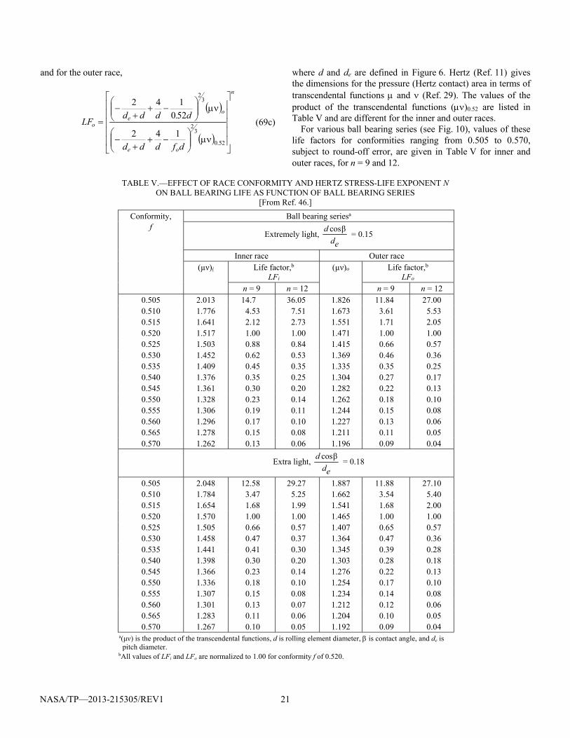
NASA/TP—2013-215305/REV1 21

and for the outer race,

n

oe

oe

o

dfddd

d.dddLF

52.0

32

32

142

520

142

(69c)

where d and de are defined in Figure 6. Hertz (Ref. 11) gives the dimensions for the pressure (Hertz contact) area in terms of transcendental functions and (Ref. 29). The values of the product of the transcendental functions ()0.52 are listed in Table V and are different for the inner and outer races.

For various ball bearing series (see Fig. 10), values of these life factors for conformities ranging from 0.505 to 0.570, subject to round-off error, are given in Table V for inner and outer races, for n = 9 and 12.

TABLE V.—EFFECT OF RACE CONFORMITY AND HERTZ STRESS-LIFE EXPONENT N

ON BALL BEARING LIFE AS FUNCTION OF BALL BEARING SERIES [From Ref. 46.]

Conformity, f

Ball bearing seriesa

Extremely light, ed

d βcos = 0.15

Inner race Outer race (µν)i Life factor,b

LFi (µν)o Life factor,b

LFo n = 9 n = 12 n = 9 n = 12

0.505 2.013 14.7 36.05 1.826 11.84 27.00 0.510 1.776 4.53 7.51 1.673 3.61 5.53 0.515 1.641 2.12 2.73 1.551 1.71 2.05 0.520 1.517 1.00 1.00 1.471 1.00 1.00 0.525 1.503 0.88 0.84 1.415 0.66 0.57 0.530 1.452 0.62 0.53 1.369 0.46 0.36 0.535 1.409 0.45 0.35 1.335 0.35 0.25 0.540 1.376 0.35 0.25 1.304 0.27 0.17 0.545 1.361 0.30 0.20 1.282 0.22 0.13 0.550 1.328 0.23 0.14 1.262 0.18 0.10 0.555 1.306 0.19 0.11 1.244 0.15 0.08 0.560 1.296 0.17 0.10 1.227 0.13 0.06 0.565 1.278 0.15 0.08 1.211 0.11 0.05 0.570 1.262 0.13 0.06 1.196 0.09 0.04

Extra light, ed

d βcos = 0.18

0.505 2.048 12.58 29.27 1.887 11.88 27.10 0.510 1.784 3.47 5.25 1.662 3.54 5.40 0.515 1.654 1.68 1.99 1.541 1.68 2.00 0.520 1.570 1.00 1.00 1.465 1.00 1.00 0.525 1.505 0.66 0.57 1.407 0.65 0.57 0.530 1.458 0.47 0.37 1.364 0.47 0.36 0.535 1.441 0.41 0.30 1.345 0.39 0.28 0.540 1.398 0.30 0.20 1.303 0.28 0.18 0.545 1.366 0.23 0.14 1.276 0.22 0.13 0.550 1.336 0.18 0.10 1.254 0.17 0.10 0.555 1.307 0.15 0.08 1.234 0.14 0.08 0.560 1.301 0.13 0.07 1.212 0.12 0.06 0.565 1.283 0.11 0.06 1.204 0.10 0.05 0.570 1.267 0.10 0.05 1.192 0.09 0.04

a(μν) is the product of the transcendental functions, d is rolling element diameter, is contact angle, and de is pitch diameter.

bAll values of LFi and LFo are normalized to 1.00 for conformity f of 0.520.

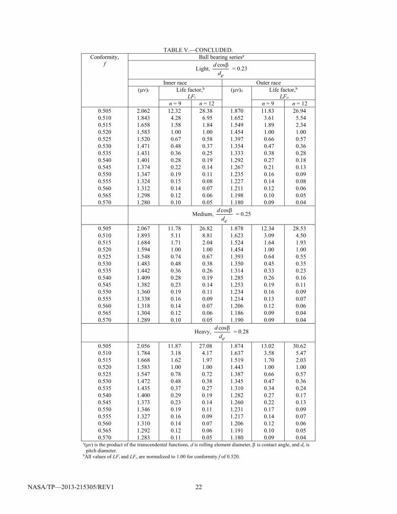
NASA/TP—2013-215305/REV1 22

TABLE V.—CONCLUDED. Conformity,

f Ball bearing seriesa

Light, ed

d βcos = 0.23

Inner race Outer race (µν)i Life factor,b

LFi

(µν)o Life factor,b LFo

n = 9 n = 12 n = 9 n = 12 0.505 2.062 12.32 28.38 1.870 11.83 26.94 0.510 1.843 4.28 6.95 1.652 3.61 5.54 0.515 1.658 1.58 1.84 1.549 1.89 2.34 0.520 1.583 1.00 1.00 1.454 1.00 1.00 0.525 1.520 0.67 0.58 1.397 0.66 0.57 0.530 1.471 0.48 0.37 1.354 0.47 0.36 0.535 1.431 0.36 0.25 1.333 0.38 0.28 0.540 1.401 0.28 0.19 1.292 0.27 0.18 0.545 1.374 0.22 0.14 1.267 0.21 0.13 0.550 1.347 0.19 0.11 1.235 0.16 0.09 0.555 1.324 0.15 0.08 1.227 0.14 0.08 0.560 1.312 0.14 0.07 1.211 0.12 0.06 0.565 1.298 0.12 0.06 1.198 0.10 0.05 0.570 1.280 0.10 0.05 1.180 0.09 0.04

Medium, ed

d βcos = 0.25

0.505 2.067 11.78 26.82 1.878 12.34 28.53 0.510 1.893 5.11 8.81 1.623 3.09 4.50 0.515 1.684 1.71 2.04 1.524 1.64 1.93 0.520 1.594 1.00 1.00 1.454 1.00 1.00 0.525 1.548 0.74 0.67 1.393 0.64 0.55 0.530 1.483 0.48 0.38 1.350 0.45 0.35 0.535 1.442 0.36 0.26 1.314 0.33 0.23 0.540 1.409 0.28 0.19 1.285 0.26 0.16 0.545 1.382 0.23 0.14 1.253 0.19 0.11 0.550 1.360 0.19 0.11 1.234 0.16 0.09 0.555 1.338 0.16 0.09 1.214 0.13 0.07 0.560 1.318 0.14 0.07 1.206 0.12 0.06 0.565 1.304 0.12 0.06 1.186 0.09 0.04 0.570 1.289 0.10 0.05 1.190 0.09 0.04

Heavy, ed

d βcos = 0.28

0.505 2.056 11.87 27.08 1.874 13.02 30.62 0.510 1.784 3.18 4.17 1.637 3.58 5.47 0.515 1.668 1.62 1.97 1.519 1.70 2.03 0.520 1.583 1.00 1.00 1.443 1.00 1.00 0.525 1.547 0.78 0.72 1.387 0.66 0.57 0.530 1.472 0.48 0.38 1.345 0.47 0.36 0.535 1.435 0.37 0.27 1.310 0.34 0.24 0.540 1.400 0.29 0.19 1.282 0.27 0.17 0.545 1.373 0.23 0.14 1.260 0.22 0.13 0.550 1.346 0.19 0.11 1.231 0.17 0.09 0.555 1.327 0.16 0.09 1.217 0.14 0.07 0.560 1.310 0.14 0.07 1.206 0.12 0.06 0.565 1.292 0.12 0.06 1.191 0.10 0.05 0.570 1.283 0.11 0.05 1.180 0.09 0.04

a(μν) is the product of the transcendental functions, d is rolling element diameter, is contact angle, and de is pitch diameter.

bAll values of LFi and LFo are normalized to 1.00 for conformity f of 0.520.

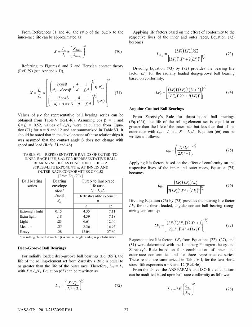
NASA/TP—2013-215305/REV1 23

From References 31 and 46, the ratio of the outer- to the inner-race life can be approximated as

n

i

o

o

i

S

S

L

LX

max

max (70)

Referring to Figures 6 and 7 and Hertzian contact theory (Ref. 29) (see Appendix D),

n

ioe

oie

i

o

dfddd

dfddd

L

LX

)(14

cos

cos2

)(14

cos

cos2

32

32

(71)

Values of for representative ball bearing series can be obtained from Table V (Ref. 46). Assuming cos = 1 and fi = fo = 0.52, values of Lo/Li were calculated from Equa-tion (71) for n = 9 and 12 and are summarized in Table VI. It should be noted that in the development of these relationships it was assumed that the contact angle does not change with speed and load (Refs. 31 and 46).

TABLE VI.—REPRESENTATIVE RATIOS OF OUTER- TO INNER-RACE LIFE, Lo/Li FOR REPRESENTATIVE BALL

BEARING SERIES AS FUNCTION OF HERTZ STRESS-LIFE EXPONENT, n, AT INNER- AND

OUTER-RACE CONFORMITIES OF 0.52 [From Eq. (70).]

Ball bearing series

Bearing envelope

size,a

ed

d βcos

Outer- to inner-race life ratio, X = Lo/Li

Hertz stress-life exponent, n

9 12

Extremely light 0.15 4.35 7.11 Extra light .18 4.39 7.18 Light .23 6.61 12.40 Medium .25 8.36 16.96 Heavy .28 12.04 27.60 ad is rolling element diameter, is contact angle, and de is pitch diameter.

Deep-Groove Ball Bearings

For radially loaded deep-groove ball bearings (Eq. (65)), the life of the rolling-element set from Zaretsky’s Rule is equal to or greater than the life of the outer race. Therefore, Lre = Lo with X = Lo/Li. Equation (65) can be rewritten as

e

e

ei

e

X

LXL

1

102

(72)

Applying life factors based on the effect of conformity to the respective lives of the inner and outer races, Equation (72) becomes

eei

eeo

ioi

LFXLF

LXLFLFL

m 110

2

(73)

Dividing Equation (73) by (72) provides the bearing life factor LFc for the radially loaded deep-groove ball bearing based on conformity:

e

ei

eeo

eo

ei

cLFXLF

XLFLFLF

1

2

2

(74)

Angular-Contact Ball Bearings

From Zaretsky’s Rule for thrust-loaded ball bearings (Eq. (66)), the life of the rolling-element set is equal to or greater than the life of the inner race but less than that of the outer race with Lre = Li and X = Lo/Li. Equation (66) can be written as follows:

e

e

ei

e

X

LXL

1

1012

(75)

Applying life factors based on the effect of conformity on the respective lives of the inner and outer races, Equation (75) becomes

eei

eeo

ioi

LFXLF

LXLFLFL

110

2

(76)

Dividing Equation (76) by (75) provides the bearing life factor LFc for the thrust-loaded, angular-contact ball bearing recog-nizing conformity:

e

ei

eeo

eeo

ei

cLFXLF

XLFLFLF

1

2

12

(77)

Representative life factors LFc from Equations (22), (27), and (31) were determined with the Lundberg-Palmgren theory and Zaretsky’s Rule based on four combinations of inner- and outer-race conformities and for three representative series. These results are summarized in Table VII, for the two Hertz stress-life exponents n = 9 and 12 (Ref. 46).

From the above, the ANSI/ABMA and ISO life calculations can be modified based upon ball-race conformity as follows:

p

eq

Dc

P

CLFL

10 (78)

NASA/TP—2013-215305/REV1 24

TABLE VII.—LIFE FACTORS BASED ON COMBINATIONS OF BALL-RACE CONFORMITIES FOR HERTZ STRESS-LIFE EXPONENT n = 9 AND 12 NORMALIZED TO INNER- AND OUTER-RACE CONFORMITIES OF 0.52

[From Ref. 46.]Ball bearing seriesa Ball-race conformity Bearing life factor for conformity,b LFc

Lundberg-Palmgrenc

Deep-groove ball bearing Angular-contact ball bearingInner race,

IR Outer race,

OR From Eq. (72) Change from

Lundberg-Palmgren,percent

From Eq. (77) Change from Lundberg-Palmgren,

percent

Hertz stress-life exponent n = 9 and L10 = 3

eq

P

CD

Extremely light,

ed

d cos = 0.15

0.505 0.57 0.52 0.52

0.52 0.52 0.505 0.57

4.16 0.15 1.16 0.35

3.15 0.15 1.19 0.22

–24.30 -------- 2.59

–37.11

7.40 0.14 1.09 0.45

–77.83 –6.59 –6.23 29.83

Light,

ed

d cos = 0.23

0.505 0.57 0.52 0.52

0.52 0.52 0.505 0.57

5.10 0.11 1.10 0.49

3.05 0.10 1.04 0.27

–40.28 –9.09 –5.68

–39.04

6.97 0.11 7.05 0.59

36.76 ------- –4.42 35.15

Heavy,

ed

d cos = 0.28

0.505 0.57 0.52 0.52

0.52 0.52 0.505 0.57

6.77 0.12 1.05 0.59

4.66 0.10 0.89 0.31

–32.24 –18.53 –15.08 –46.87

8.51 0.09 1.03 0.73

25.73 –26.03

–2.22 24.15

Hertz stress-life exponent n = 12 and L10 =

4

eq

P

CD

Extremely light,

ed

d cos = 0.15

0.505 0.52 6.83

eqP

CD 3.65

eqP

CD –46.56 10.79

eqP

CD 57.98

0.57 0.52 0.07

eqP

CD 0.06

eqP

CD –14.29 0.06

eqP

CD –14.29

0.52 0.505 1.10

eqP

CD 1.02

eqP

CD –7.27 1.05

eqP

CD –4.55

0.52 0.57 0.26

eqP

CD 0.14

eqP

CD –46.15 0.39

eqP

CD 50.00

Light,

ed

d cos = 0.23

0.505 0.52 9.67

eqP

CD 5.03

eqP

CD –47.98 14.03

eqP

CD 45.09

0.57 0.52 0.05

eqP

CD 0.04

eqP

CD –20.00 0.05

eqP

CD --------

0.52 0.505 1.05

eqP

CD 0.89

eqP

CD –15.24 1.03

eqP

CD –1.90

0.52 0.57 0.37

eqP

CD 0.20

eqP

CD –45.95 0.53

eqP

CD 43.24

Heavy,

ed

d cos = 0.28

0.505 0.52 14.97

eqP

CD 7.81

eqP

CD –47.83 19.13

eqP

CD 27.79

0.57 0.52 0.05

eqP

CD 0.04

eqP

CD –20.00 0.05

eqP

CD -------

0.52 0.505 1.02

eqP

CD 0.77

eqP

CD –24.51 1.01

eqP

CD –0.01

0.52 0.57 0.57

eqP

CD 0.30

eqP

CD –47.37 0.72

eqP

CD 26.32

ad is rolling element diameter, is contact angle, and de is pitch diameter.

bAll life factors are benchmarked to inner- and outer-race conformities of 0.52 and L10 = 3

eq

P

CD where CD is bearing dynamic capacity and Peq is equivalent load.

cFor deep-groove and angular-contact ball bearings.

NASA/TP—2013-215305/REV1 25

The bearing fatigue lives in actual application will usually be equal to or greater than those calculated using the ANSI/ABMA and ISO standards that incorporate the Lundberg-Palmgren model. The relative fatigue life of an individual race is more sensitive to changes in race conformity for a Hertz stress-life exponent n of 12 than where n = 9. However, when the effects are combined to predict actual bearing life for a specified set of conditions and bearing geometry, the predicted life of the bearing will be greater for a value of n = 12 (p = 4) than n = 9 (p = 3) (Ref. 46).

Stress Effects

Hertz Stress-Life Relation

There is an issue of what the value of the Hertz stress-life relation and, hence, the value of the load-life exponent p should be for purposes of analysis. The generally accepted relation between load and life in a rolling-element bearing is that life varies with the inverse cubic power of load for ball bearings (point contact) and with the inverse 4th power of load for roller bearings (line contact). Work reported by Parker and Zaretsky (Ref. 47) suggests that for air-melted steels the stress-life exponent n is approximately 9 for point contact. However, for the cleaner post-1960 vacuum-processed steels, n = 12 for point contact better fits the data. A definitive database does not exist for line contact (roller bearings).

For ball bearings, the Hertz stress-life relation where life is inversely proportional to the maximum Hertz stress to the 9th power and the cubic root of load, has been generally accepted by ball bearing manufacturers and users. There is at least one exception where a manufacturer had indicated based on its unpublished database that the life of ball bearings varies inversely with the 4th power of load (or 12th power of Hertz stress). Nevertheless, the inverse cubic load-life relation has been included in the ANSI/ABMA standards for ball bearings (Ref. 13).

Varying the Hertz stress-life exponent n can significantly affect life predictions for long-lived (lightly loaded) bearings. Using n = 9 results in a more conservative estimate of bearing life than using n = 12. Also, the ratio of the predicted lives at the two values of the Hertz stress-life exponent n is a function of load and is directly related to CD/Peq. Hence, in the normal operating load envelope, life may be underpredicted by a factor of 20 when using the ANSI/ABMA standards or a 9th power Hertz stress-life exponent n. A proper stress-life exponent then becomes more than of mere academic interest, since a design engineer requires a reliable analytic tool to predict bearing life and performance.

Fatigue tests of ball bearings by several investigators tended to verify this inverse cubic relation. Styri (Ref. 48) presented data for two types of ball bearings. For one group of 6207-size, deep-groove ball bearings under various radial loads from 3.5 to

17.3 kN (775 to 3880 lbf), life was inversely proportional to load to the 3.3 power. Another group of 1207-size double-row self-aligning bearings was tested with very high load such that the maximum Hertz stress at the outer-race-ball contact varied from 4.0 to 5.6 GPa (580 to 810 ksi). Here it was found that life varied inversely with the 9th power of stress (or the 3rd power of load). Cordiano et al. (Ref. 49) reported load-life data for 217-size, thrust-loaded ball bearings. The resultant Hertz stress-life exponents were 8.1, 9.6, and 12.6 for three lubricants, a water-glycol base, a phosphate ester base, and a phosphate ester, respectively. McKelvey and Moyer (Ref. 50) reported that with four groups of AISI 4620, carburized-steel, crowned rollers (elliptical contact), fatigue life varied inversely with maximum Hertz stress to a range of the 8th to 9th power. Maximum Hertz stress in these tests varied from 1.8 to 3.3 GPa (262 to 478 ksi). Townsend et al. (Ref. 51) surface fatigue tested three groups of case-carburized, consumable-electrode-vacuum-arc-remelted AISI 9310 8.89-cm- (3.5-in.-) pitch-diameter spur gears at maximum Hertz stresses of 1.5, 1.7, and 1.9 GPa (222, 248, and 272 ksi). The gears were run at 10 000 rpm and 77 °C (170 °F). The lubricant was superrefined naphthenic mineral oil with an additive package. The L10 life varied inversely with stress to the 8.4 power, but the L50 life varied inversely with stress to the 10.2 power. The average Hertz stress-life exponent n was 9.3.

Several other investigators (Refs. 52 to 60) have reported data with bench-type, rolling-element fatigue testers, rather than with full-scale bearings or gears. Data are summarized in Table VIII. The L10 lives as a function of maximum Hertz stress for these data are shown in Figure 11. From the table the maximum Hertz stress for these data ranged from 3.7 to 9.0 GPa (526 to 1300 ksi). With the exception of Greenert’s work (Ref. 57) the stress-life exponents ranged from 8.4 to 12.4. The data are all for AISI 52100 and AISI M–50 steels (except for the data reported by Barwell and Scott (Ref. 52), who do not state the type of steel). At least two sets of data were for air-melted steel, three were for vacuum-degassed steel, and one was for vacuum-arc-remelted steel. The other references do not state the melting process.

The Hertz stress-life exponents from Greenert (Ref. 57), ranging from 15 to 19, are much higher than those from other published data. This lack of correlation is unexplained. However, there is a probability that compressive residual stresses present in the AISI 52100 steel could account for the resultant high values of the Hertz stress-life exponents.

Lorosch (Ref. 61) fatigue tested three groups of vacuum-degassed 7205B-size AISI 52100 inner races at maximum Hertz stresses of 2.6, 2.8, and 3.5 GPa (370, 406, and 500 ksi). Each group consisted of 20 races, for a total of 60. (It is assumed that all 60 races came from a single heat of material and were of the same hardness, but Lorosch does not state so in his paper.) After the test runs Lorosch examined cross sections of the races. He observed that only at the lowest stress, 2.6 GPa (370 ksi), did no measurable plastic deformation occur. At the two higher stresses

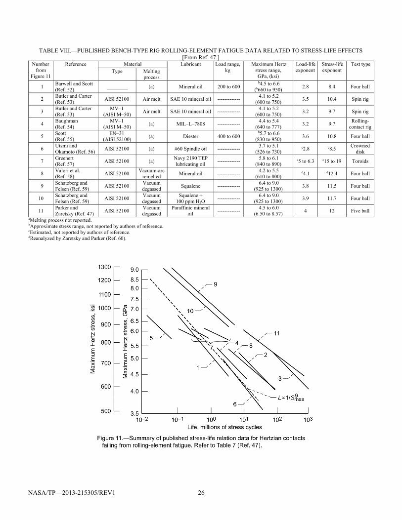
NASA/TP—2013-215305/REV1 26

TABLE VIII.—PUBLISHED BENCH-TYPE RIG ROLLING-ELEMENT FATIGUE DATA RELATED TO STRESS-LIFE EFFECTS [From Ref. 47.]

Number from

Figure 11

Reference Material Lubricant Load range, kg

Maximum Hertz stress range, GPa, (ksi)

Load-life exponent

Stress-life exponent

Test type Type Melting

process

1 Barwell and Scott (Ref. 52)

________ (a) Mineral oil 200 to 600 b4.5 to 6.6

(b660 to 950) 2.8 8.4 Four ball

2 Butler and Carter (Ref. 53)

AISI 52100 Air melt SAE 10 mineral oil ------------- 4.1 to 5.2

(600 to 750) 3.5 10.4 Spin rig

3 Butler and Carter (Ref. 53)

MV–1 (AISI M–50)

Air melt SAE 10 mineral oil ------------- 4.1 to 5.2

(600 to 750) 3.2 9.7 Spin rig

4 Baughman (Ref. 54)

MV–1 (AISI M–50)

(a) MIL–L–7808 ------------- 4.4 to 5.4

(640 to 777) 3.2 9.7

Rolling-contact rig

5 Scott (Ref. 55)

EN–31 (AISI 52100)

(a) Diester 400 to 600 b5.7 to 6.6

(830 to 950) 3.6 10.8 Four ball

6 Utsmi and Okamoto (Ref. 56)

AISI 52100 (a) #60 Spindle oil ------------- 3.7 to 5.1

(526 to 730) c2.8 c8.5

Crowned disk

7 Greenert (Ref. 57)

AISI 52100 (a) Navy 2190 TEP lubricating oil

------------- 5.8 to 6.1

(840 to 890) c5 to 6.3 c15 to 19 Toroids

8 Valori et al. (Ref. 58)

AISI 52100 Vacuum-arc

remelted Mineral oil -------------

4.2 to 5.5 (610 to 800)

d4.1 d12.4 Four ball

9 Schatzberg and Felsen (Ref. 59)

AISI 52100 Vacuum degassed

Squalene ------------- 6.4 to 9.0

(925 to 1300) 3.8 11.5 Four ball

10 Schatzberg and Felsen (Ref. 59)

AISI 52100 Vacuum degassed

Squalene + 100 ppm H2O

------------- 6.4 to 9.0

(925 to 1300) 3.9 11.7 Four ball

11 Parker and Zaretsky (Ref. 47)

AISI 52100 Vacuum degassed

Paraffinic mineral oil

------------- 4.5 to 6.0

(6.50 to 8.57) 4 12 Five ball

aMelting process not reported. bApproximate stress range, not reported by authors of reference. cEstimated, not reported by authors of reference. dReanalyzed by Zaretsky and Parker (Ref. 60).

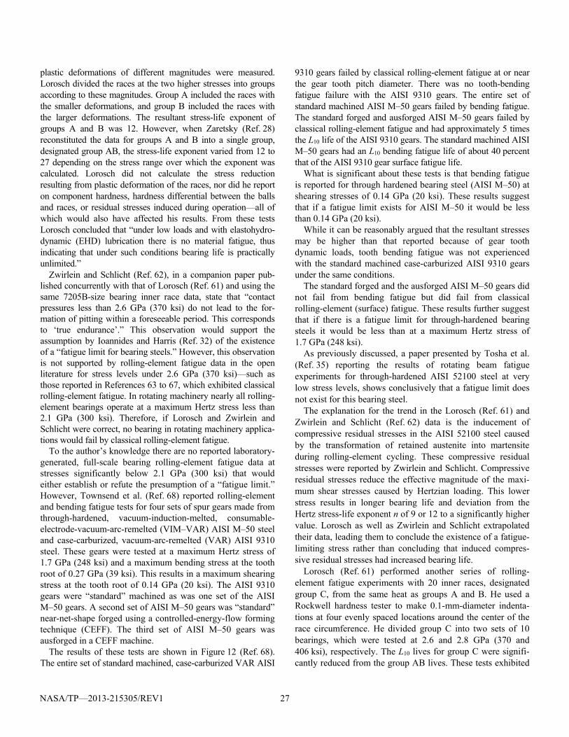
NASA/TP—2013-215305/REV1 27

plastic deformations of different magnitudes were measured. Lorosch divided the races at the two higher stresses into groups according to these magnitudes. Group A included the races with the smaller deformations, and group B included the races with the larger deformations. The resultant stress-life exponent of groups A and B was 12. However, when Zaretsky (Ref. 28) reconstituted the data for groups A and B into a single group, designated group AB, the stress-life exponent varied from 12 to 27 depending on the stress range over which the exponent was calculated. Lorosch did not calculate the stress reduction resulting from plastic deformation of the races, nor did he report on component hardness, hardness differential between the balls and races, or residual stresses induced during operation—all of which would also have affected his results. From these tests Lorosch concluded that “under low loads and with elastohydro-dynamic (EHD) lubrication there is no material fatigue, thus indicating that under such conditions bearing life is practically unlimited.”

Zwirlein and Schlicht (Ref. 62), in a companion paper pub-lished concurrently with that of Lorosch (Ref. 61) and using the same 7205B-size bearing inner race data, state that “contact pressures less than 2.6 GPa (370 ksi) do not lead to the for-mation of pitting within a foreseeable period. This corresponds to ‘true endurance’.” This observation would support the assumption by Ioannides and Harris (Ref. 32) of the existence of a “fatigue limit for bearing steels.” However, this observation is not supported by rolling-element fatigue data in the open literature for stress levels under 2.6 GPa (370 ksi)—such as those reported in References 63 to 67, which exhibited classical rolling-element fatigue. In rotating machinery nearly all rolling-element bearings operate at a maximum Hertz stress less than 2.1 GPa (300 ksi). Therefore, if Lorosch and Zwirlein and Schlicht were correct, no bearing in rotating machinery applica-tions would fail by classical rolling-element fatigue.

To the author’s knowledge there are no reported laboratory-generated, full-scale bearing rolling-element fatigue data at stresses significantly below 2.1 GPa (300 ksi) that would either establish or refute the presumption of a “fatigue limit.” However, Townsend et al. (Ref. 68) reported rolling-element and bending fatigue tests for four sets of spur gears made from through-hardened, vacuum-induction-melted, consumable-electrode-vacuum-arc-remelted (VIM–VAR) AISI M–50 steel and case-carburized, vacuum-arc-remelted (VAR) AISI 9310 steel. These gears were tested at a maximum Hertz stress of 1.7 GPa (248 ksi) and a maximum bending stress at the tooth root of 0.27 GPa (39 ksi). This results in a maximum shearing stress at the tooth root of 0.14 GPa (20 ksi). The AISI 9310 gears were “standard” machined as was one set of the AISI M–50 gears. A second set of AISI M–50 gears was “standard” near-net-shape forged using a controlled-energy-flow forming technique (CEFF). The third set of AISI M–50 gears was ausforged in a CEFF machine.

The results of these tests are shown in Figure 12 (Ref. 68). The entire set of standard machined, case-carburized VAR AISI

9310 gears failed by classical rolling-element fatigue at or near the gear tooth pitch diameter. There was no tooth-bending fatigue failure with the AISI 9310 gears. The entire set of standard machined AISI M–50 gears failed by bending fatigue. The standard forged and ausforged AISI M–50 gears failed by classical rolling-element fatigue and had approximately 5 times the L10 life of the AISI 9310 gears. The standard machined AISI M–50 gears had an L10 bending fatigue life of about 40 percent that of the AISI 9310 gear surface fatigue life.

What is significant about these tests is that bending fatigue is reported for through hardened bearing steel (AISI M–50) at shearing stresses of 0.14 GPa (20 ksi). These results suggest that if a fatigue limit exists for AISI M–50 it would be less than 0.14 GPa (20 ksi).

While it can be reasonably argued that the resultant stresses may be higher than that reported because of gear tooth dynamic loads, tooth bending fatigue was not experienced with the standard machined case-carburized AISI 9310 gears under the same conditions.

The standard forged and the ausforged AISI M–50 gears did not fail from bending fatigue but did fail from classical rolling-element (surface) fatigue. These results further suggest that if there is a fatigue limit for through-hardened bearing steels it would be less than at a maximum Hertz stress of 1.7 GPa (248 ksi).

As previously discussed, a paper presented by Tosha et al. (Ref. 35) reporting the results of rotating beam fatigue experiments for through-hardened AISI 52100 steel at very low stress levels, shows conclusively that a fatigue limit does not exist for this bearing steel.

The explanation for the trend in the Lorosch (Ref. 61) and Zwirlein and Schlicht (Ref. 62) data is the inducement of compressive residual stresses in the AISI 52100 steel caused by the transformation of retained austenite into martensite during rolling-element cycling. These compressive residual stresses were reported by Zwirlein and Schlicht. Compressive residual stresses reduce the effective magnitude of the maxi-mum shear stresses caused by Hertzian loading. This lower stress results in longer bearing life and deviation from the Hertz stress-life exponent n of 9 or 12 to a significantly higher value. Lorosch as well as Zwirlein and Schlicht extrapolated their data, leading them to conclude the existence of a fatigue-limiting stress rather than concluding that induced compres-sive residual stresses had increased bearing life.

Lorosch (Ref. 61) performed another series of rolling-element fatigue experiments with 20 inner races, designated group C, from the same heat as groups A and B. He used a Rockwell hardness tester to make 0.1-mm-diameter indenta-tions at four evenly spaced locations around the center of the race circumference. He divided group C into two sets of 10 bearings, which were tested at 2.6 and 2.8 GPa (370 and 406 ksi), respectively. The L10 lives for group C were signifi-cantly reduced from the group AB lives. These tests exhibited

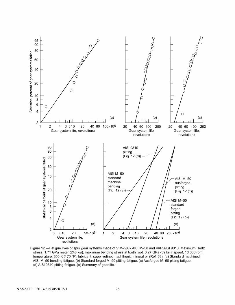
NASA/TP—2013-215305/REV1 28

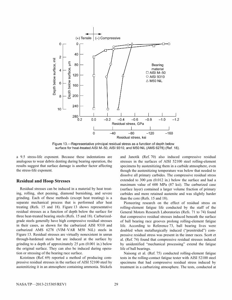
NASA/TP—2013-215305/REV1 29

a 9.5 stress-life exponent. Because these indentations are analogous to wear debris denting during bearing operation, the results suggest that surface damage is another factor affecting the stress-life exponent.

Residual and Hoop Stresses

Residual stresses can be induced in a material by heat treat-ing, rolling, shot peening, diamond burnishing, and severe grinding. Each of these methods (except heat treating) is a separate mechanical process that is performed after heat treating (Refs. 15 and 18). Figure 13 shows representative residual stresses as a function of depth below the surface for three heat-treated bearing steels (Refs. 15 and 18). Carburized-grade steels generally have high compressive residual stresses in their cases, as shown for the carburized AISI 9310 and carburized AMS 6278 (VIM–VAR M50 NiL) steels in Figure 13. Residual stresses are virtually nonexistent in unrun through-hardened steels but are induced at the surface by grinding to a depth of approximately 25 m (0.001 in.) below the original surface. They can also be induced during opera-tion or stressing of the bearing race surface.

Koistinen (Ref. 69) reported a method of producing com-pressive residual stresses in the surface of AISI 52100 steel by austenitizing it in an atmosphere containing ammonia. Stickels

and Janotik (Ref. 70) also induced compressive residual stresses in the surfaces of AISI 52100 steel rolling-element specimens by austenitizing them in a carbide atmosphere, even though the austenitizing temperature was below that needed to dissolve all primary carbides. The compressive residual stress extended to 300 m (0.012 in.) below the surface and had a maximum value of 600 MPa (87 ksi). The carburized case (surface layer) contained a larger volume fraction of primary carbides and more retained austenite and was slightly harder than the core (Refs. 15 and 18).

Pioneering research on the effect of residual stress on rolling-element fatigue life conducted by the staff of the General Motors Research Laboratories (Refs. 71 to 74) found that compressive residual stresses induced beneath the surface of ball bearing race grooves prolong rolling-element fatigue life. According to Reference 73, ball bearing lives were doubled when metallurgically induced (“prenitrided”) com-pressive residual stress was present in the inner races. Scott et al. (Ref. 74) found that compressive residual stresses induced by unidentified “mechanical processing” extend the fatigue life of ball bearings.

Naisong et al. (Ref. 75) conducted rolling-element fatigue tests in the rolling-contact fatigue tester with AISI 52100 steel specimens that had compressive residual stress induced by treatment in a carburizing atmosphere. The tests, conducted at

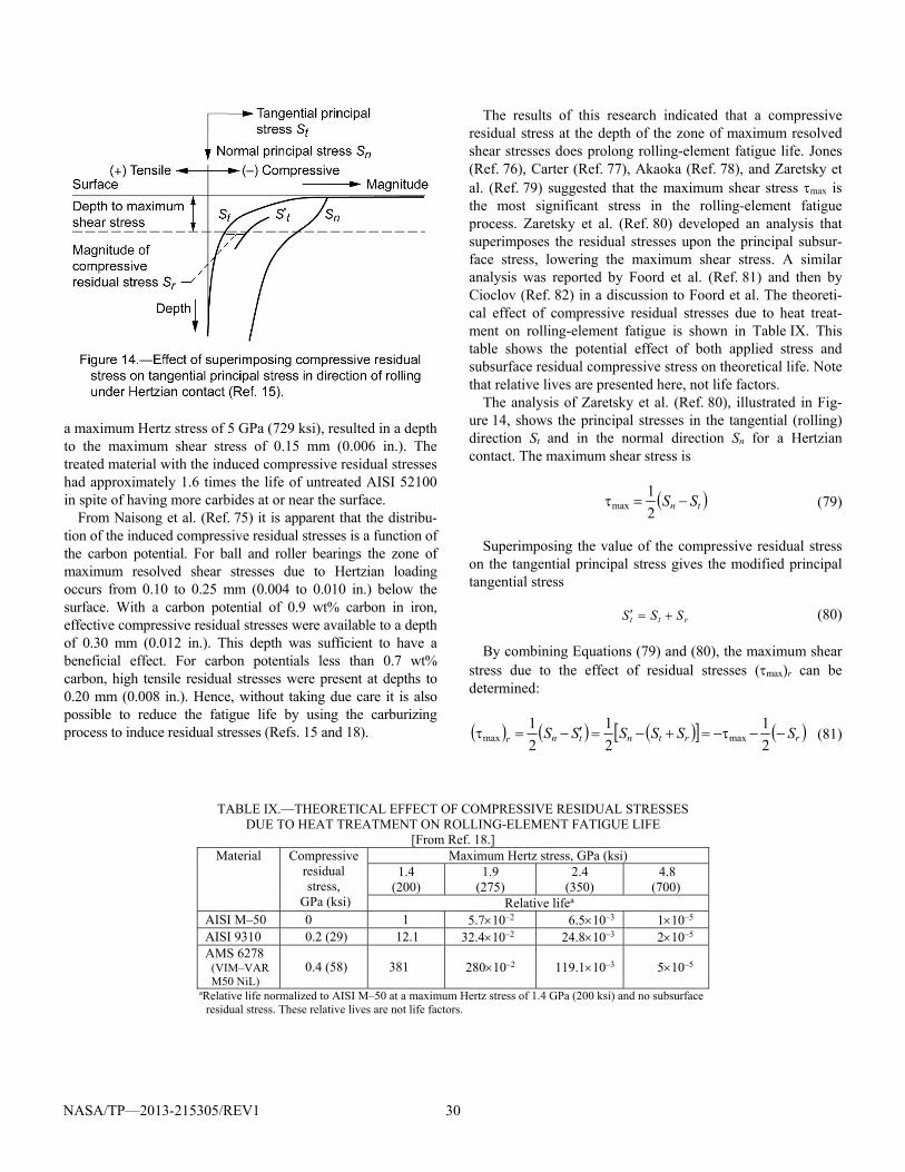
NASA/TP—2013-215305/REV1 30

a maximum Hertz stress of 5 GPa (729 ksi), resulted in a depth to the maximum shear stress of 0.15 mm (0.006 in.). The treated material with the induced compressive residual stresses had approximately 1.6 times the life of untreated AISI 52100 in spite of having more carbides at or near the surface.

From Naisong et al. (Ref. 75) it is apparent that the distribu-tion of the induced compressive residual stresses is a function of the carbon potential. For ball and roller bearings the zone of maximum resolved shear stresses due to Hertzian loading occurs from 0.10 to 0.25 mm (0.004 to 0.010 in.) below the surface. With a carbon potential of 0.9 wt% carbon in iron, effective compressive residual stresses were available to a depth of 0.30 mm (0.012 in.). This depth was sufficient to have a beneficial effect. For carbon potentials less than 0.7 wt% carbon, high tensile residual stresses were present at depths to 0.20 mm (0.008 in.). Hence, without taking due care it is also possible to reduce the fatigue life by using the carburizing process to induce residual stresses (Refs. 15 and 18).

The results of this research indicated that a compressive residual stress at the depth of the zone of maximum resolved shear stresses does prolong rolling-element fatigue life. Jones (Ref. 76), Carter (Ref. 77), Akaoka (Ref. 78), and Zaretsky et al. (Ref. 79) suggested that the maximum shear stress max is the most significant stress in the rolling-element fatigue process. Zaretsky et al. (Ref. 80) developed an analysis that superimposes the residual stresses upon the principal subsur-face stress, lowering the maximum shear stress. A similar analysis was reported by Foord et al. (Ref. 81) and then by Cioclov (Ref. 82) in a discussion to Foord et al. The theoreti-cal effect of compressive residual stresses due to heat treat-ment on rolling-element fatigue is shown in Table IX. This table shows the potential effect of both applied stress and subsurface residual compressive stress on theoretical life. Note that relative lives are presented here, not life factors.

The analysis of Zaretsky et al. (Ref. 80), illustrated in Fig-ure 14, shows the principal stresses in the tangential (rolling) direction St and in the normal direction Sn for a Hertzian contact. The maximum shear stress is

tn SS 2

1max (79)

Superimposing the value of the compressive residual stress on the tangential principal stress gives the modified principal tangential stress

rtt SSS (80)

By combining Equations (79) and (80), the maximum shear stress due to the effect of residual stresses (max)r can be determined:

rrtntnr SSSSSS 2

1

2

1

2

1maxmax (81)

TABLE IX.—THEORETICAL EFFECT OF COMPRESSIVE RESIDUAL STRESSES DUE TO HEAT TREATMENT ON ROLLING-ELEMENT FATIGUE LIFE

[From Ref. 18.] Material Compressive

residual stress,

GPa (ksi)

Maximum Hertz stress, GPa (ksi) 1.4

(200) 1.9

(275) 2.4

(350) 4.8

(700) Relative lifea

AISI M–50 0 1 5.710–2 6.510–3 110–5

AISI 9310 0.2 (29) 12.1 32.410–2 24.810–3 210–5 AMS 6278

(VIM–VAR M50 NiL)

0.4 (58) 381 28010–2 119.110–3 510–5

aRelative life normalized to AISI M–50 at a maximum Hertz stress of 1.4 GPa (200 ksi) and no subsurface residual stress. These relative lives are not life factors.

NASA/TP—2013-215305/REV1 31

The negative sign before Sr designates a compressive resid-ual stress. A positive sign before Sr would designate a tensile residual stress (Ref. 80). Hence, the residual stress can either increase or decrease the maximum shear stress. Accordingly, a compressive residual stress would reduce the maximum shear stress and increase the fatigue life according to the inverse relation of life and stress to the c/e power:

ec

r

L

/

max

1~

(82a)

for Lundberg and Palmgren where c/e = 9.3, or

c

r

L

max

1~ (82b)

for Zaretsky where 9 c 10. For rolling-element bearings the beneficial effect of the

compressive residual stresses is offset by the presence of tensile (hoop) stresses in the bearing inner race.

These hoop stresses are induced and affected primarily by the press fit of the inner race over the shaft, centrifugal loading, and thermal effects between the race and the shaft. Coe and Zaretsky (Ref. 83) analyzed the effect of hoop stresses on rolling-element fatigue. Czyzewski (Ref. 84) showed that, in the absence of compressive residual stress, hoop stresses are generally tensile, are designated by a + sign, and can negatively affect fatigue life. As with the compressive residual stresses, hoop stresses alter the critical subsurface shear stress and affect the life of the bearing inner race. Equation (81) can be rewritten to account for the effect of both residual and tensile (hoop) stresses as

hrrh SS 2

1maxmax (83)

Again the positive or negative sign indicates a tensile or compressive stress, respectively. Equation (82) can be written to reflect the effect of both the compressive and tensile stresses on life. For Lundberg and Palmgren, where c/e = 9.3, this is

ec

hr

L

/

max

1~

(84a)

or for Zaretsky, where 9 c 10, this is

c

rh

L

max

1~ (84b)

Since life ec

L/

1~

or c

1

, Equations (48) and (84)

have been combined to modify the predicted bearing life (Ref. 18). From Lundberg and Palmgren (Ref. 9),

p

eq

D

ec

rh P

CL

/

max

max10 (85a)

where c/e = 9.3, p = 3 for ball bearings, and p = 4 for roller bearings. From Zaretsky,

p

eq

D

c

rh P

CL

max

max10 (85b)

where p = 4 for ball bearings, p = 5 for roller bearings, and 9 c 10. From Hertz theory (Ref. 29), max 0.32Smax for ball bearings, depending on raceway conformity, and 0.3Smax for roller bearings.

Comparison of Bearing Life Models The Ioannides-Harris model without a fatigue limit is identi-

cal to the Lundberg-Palmgren model. The Weibull model is similar to that of Zaretsky if the exponents are chosen to be identical. Comparison of the Lundberg-Palmgren model and the Zaretsky model with the ANSI/ABMA and ISO standards is shown in Figure 15 for ball and cylindrical roller bearings. The theoretical lives were normalized to a maximum Hertz stress of 4.14 GPa (600 ksi) and subsequently normalized to the calculat-ed ANSI/ABMA and ISO standards at each stress level. For the Ioannides-Harris comparison shown in Figure 15, a fatigue-limiting stress of 276 MPa (40 ksi) was assumed. For ball bearings, the ANSI/ABMA and ISO standards and the Lundberg-Palmgren model give identical results. For roller bearings, the results are not identical (Ref. 85).

The ANSI/ABMA and ISO standards use a load-life expo-nent p of 10/3 (3.33) for line contact (roller bearings). This results in a value of n equal to 6.6 and can account in part for lower life predictions than those experienced in the field. From Lundberg and Palmgren (Ref. 9), the load-life exponent p for line contact should be 4. However, Lundberg and Palmgren’s justification for a p of 10/3 was that a roller bearing can experience “mixed contact”; that is, one raceway can experience line contact and the other raceway point contact (Ref. 10). This may be true in a limited number of roller bearing designs, but it is certainly not consistent with the vast majority of cylindrical roller and tapered roller bearings designed and used today.

Both the load-life and stress-life relations of Weibull, Lundberg and Palmgren, and Ioannides and Harris reflect a strong dependence on the Weibull slope. The existing

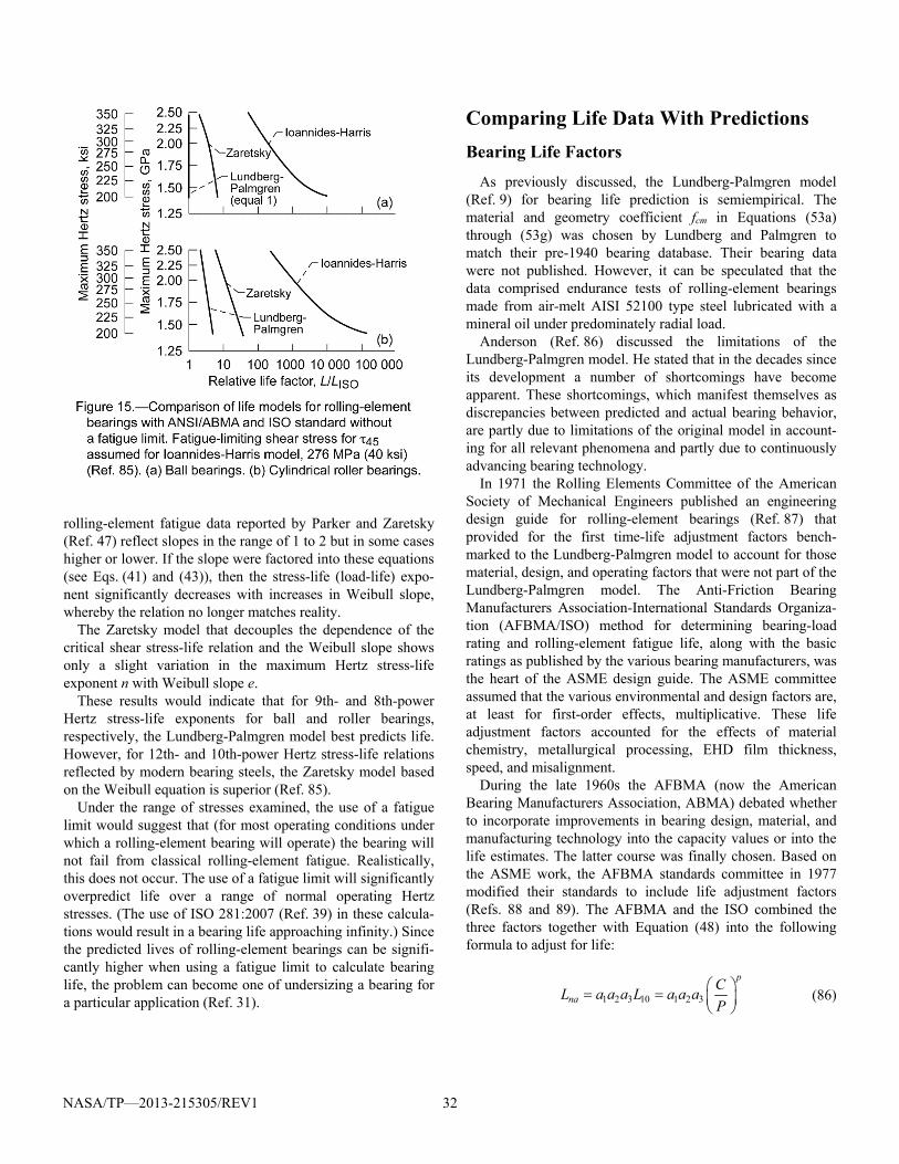
NASA/TP—2013-215305/REV1 32

rolling-element fatigue data reported by Parker and Zaretsky (Ref. 47) reflect slopes in the range of 1 to 2 but in some cases higher or lower. If the slope were factored into these equations (see Eqs. (41) and (43)), then the stress-life (load-life) expo-nent significantly decreases with increases in Weibull slope, whereby the relation no longer matches reality.

The Zaretsky model that decouples the dependence of the critical shear stress-life relation and the Weibull slope shows only a slight variation in the maximum Hertz stress-life exponent n with Weibull slope e.

These results would indicate that for 9th- and 8th-power Hertz stress-life exponents for ball and roller bearings, respectively, the Lundberg-Palmgren model best predicts life. However, for 12th- and 10th-power Hertz stress-life relations reflected by modern bearing steels, the Zaretsky model based on the Weibull equation is superior (Ref. 85).

Under the range of stresses examined, the use of a fatigue limit would suggest that (for most operating conditions under which a rolling-element bearing will operate) the bearing will not fail from classical rolling-element fatigue. Realistically, this does not occur. The use of a fatigue limit will significantly overpredict life over a range of normal operating Hertz stresses. (The use of ISO 281:2007 (Ref. 39) in these calcula-tions would result in a bearing life approaching infinity.) Since the predicted lives of rolling-element bearings can be signifi-cantly higher when using a fatigue limit to calculate bearing life, the problem can become one of undersizing a bearing for a particular application (Ref. 31).

Comparing Life Data With Predictions

Bearing Life Factors

As previously discussed, the Lundberg-Palmgren model (Ref. 9) for bearing life prediction is semiempirical. The material and geometry coefficient fcm in Equations (53a) through (53g) was chosen by Lundberg and Palmgren to match their pre-1940 bearing database. Their bearing data were not published. However, it can be speculated that the data comprised endurance tests of rolling-element bearings made from air-melt AISI 52100 type steel lubricated with a mineral oil under predominately radial load.

Anderson (Ref. 86) discussed the limitations of the Lundberg-Palmgren model. He stated that in the decades since its development a number of shortcomings have become apparent. These shortcomings, which manifest themselves as discrepancies between predicted and actual bearing behavior, are partly due to limitations of the original model in account-ing for all relevant phenomena and partly due to continuously advancing bearing technology.

In 1971 the Rolling Elements Committee of the American Society of Mechanical Engineers published an engineering design guide for rolling-element bearings (Ref. 87) that provided for the first time-life adjustment factors bench-marked to the Lundberg-Palmgren model to account for those material, design, and operating factors that were not part of the Lundberg-Palmgren model. The Anti-Friction Bearing Manufacturers Association-International Standards Organiza-tion (AFBMA/ISO) method for determining bearing-load rating and rolling-element fatigue life, along with the basic ratings as published by the various bearing manufacturers, was the heart of the ASME design guide. The ASME committee assumed that the various environmental and design factors are, at least for first-order effects, multiplicative. These life adjustment factors accounted for the effects of material chemistry, metallurgical processing, EHD film thickness, speed, and misalignment.

During the late 1960s the AFBMA (now the American Bearing Manufacturers Association, ABMA) debated whether to incorporate improvements in bearing design, material, and manufacturing technology into the capacity values or into the life estimates. The latter course was finally chosen. Based on the ASME work, the AFBMA standards committee in 1977 modified their standards to include life adjustment factors (Refs. 88 and 89). The AFBMA and the ISO combined the three factors together with Equation (48) into the following formula to adjust for life:

1 2 3 10 1 2 3

p

naC

L a a a L a a aP

(86)

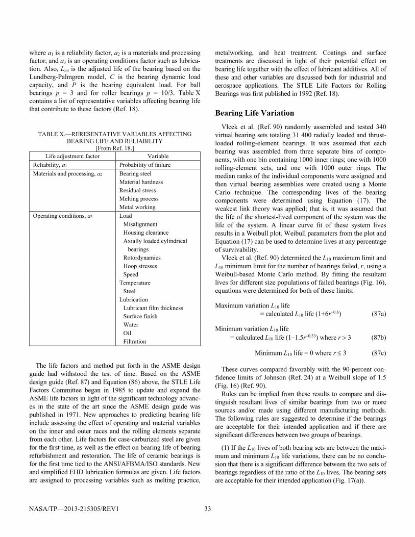
NASA/TP—2013-215305/REV1 33

where a1 is a reliability factor, a2 is a materials and processing factor, and a3 is an operating conditions factor such as lubrica-tion. Also, Lna is the adjusted life of the bearing based on the Lundberg-Palmgren model, C is the bearing dynamic load capacity, and P is the bearing equivalent load. For ball bearings p = 3 and for roller bearings p = 10/3. Table X contains a list of representative variables affecting bearing life that contribute to these factors (Ref. 18).

TABLE X.RERESENTATIVE VARIABLES AFFECTING BEARING LIFE AND RELIABILITY

[From Ref. 18.] Life adjustment factor Variable

Reliability, a1 Probability of failure

Materials and processing, a2 Bearing steel Material hardness Residual stress Melting process Metal working

Operating conditions, a3 Load Misalignment Housing clearance Axially loaded cylindrical bearings Rotordynamics Hoop stresses Speed Temperature Steel Lubrication Lubricant film thickness Surface finish Water Oil Filtration

The life factors and method put forth in the ASME design guide had withstood the test of time. Based on the ASME design guide (Ref. 87) and Equation (86) above, the STLE Life Factors Committee began in 1985 to update and expand the ASME life factors in light of the significant technology advanc-es in the state of the art since the ASME design guide was published in 1971. New approaches to predicting bearing life include assessing the effect of operating and material variables on the inner and outer races and the rolling elements separate from each other. Life factors for case-carburized steel are given for the first time, as well as the effect on bearing life of bearing refurbishment and restoration. The life of ceramic bearings is for the first time tied to the ANSI/AFBMA/ISO standards. New and simplified EHD lubrication formulas are given. Life factors are assigned to processing variables such as melting practice,

metalworking, and heat treatment. Coatings and surface treatments are discussed in light of their potential effect on bearing life together with the effect of lubricant additives. All of these and other variables are discussed both for industrial and aerospace applications. The STLE Life Factors for Rolling Bearings was first published in 1992 (Ref. 18).

Bearing Life Variation

Vlcek et al. (Ref. 90) randomly assembled and tested 340 virtual bearing sets totaling 31 400 radially loaded and thrust-loaded rolling-element bearings. It was assumed that each bearing was assembled from three separate bins of compo-nents, with one bin containing 1000 inner rings; one with 1000 rolling-element sets, and one with 1000 outer rings. The median ranks of the individual components were assigned and then virtual bearing assemblies were created using a Monte Carlo technique. The corresponding lives of the bearing components were determined using Equation (17). The weakest link theory was applied; that is, it was assumed that the life of the shortest-lived component of the system was the life of the system. A linear curve fit of these system lives results in a Weibull plot. Weibull parameters from the plot and Equation (17) can be used to determine lives at any percentage of survivability.

Vlcek et al. (Ref. 90) determined the L10 maximum limit and L10 minimum limit for the number of bearings failed, r, using a Weibull-based Monte Carlo method. By fitting the resultant lives for different size populations of failed bearings (Fig. 16), equations were determined for both of these limits:

Maximum variation L10 life = calculated L10 life (1+6r–0.6) (87a)

Minimum variation L10 life = calculated L10 life (1–1.5r–0.33) where r 3 (87b)

Minimum L10 life = 0 where r 3 (87c)

These curves compared favorably with the 90-percent con-fidence limits of Johnson (Ref. 24) at a Weibull slope of 1.5 (Fig. 16) (Ref. 90).

Rules can be implied from these results to compare and dis-tinguish resultant lives of similar bearings from two or more sources and/or made using different manufacturing methods. The following rules are suggested to determine if the bearings are acceptable for their intended application and if there are significant differences between two groups of bearings.

(1) If the L10 lives of both bearing sets are between the maxi-mum and minimum L10 life variations, there can be no conclu-sion that there is a significant difference between the two sets of bearings regardless of the ratio of the L10 lives. The bearing sets are acceptable for their intended application (Fig. 17(a)).

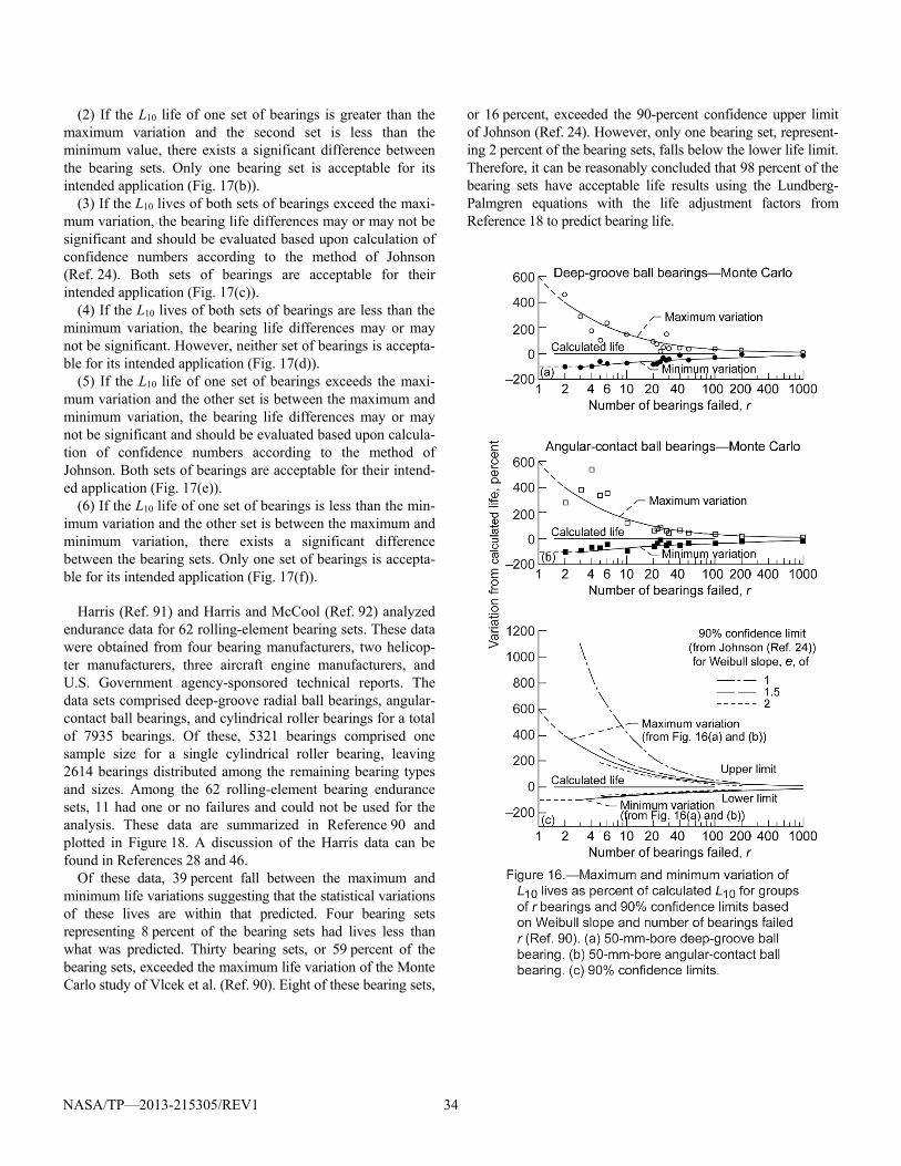
NASA/TP—2013-215305/REV1 34

(2) If the L10 life of one set of bearings is greater than the maximum variation and the second set is less than the minimum value, there exists a significant difference between the bearing sets. Only one bearing set is acceptable for its intended application (Fig. 17(b)).

(3) If the L10 lives of both sets of bearings exceed the maxi-mum variation, the bearing life differences may or may not be significant and should be evaluated based upon calculation of confidence numbers according to the method of Johnson (Ref. 24). Both sets of bearings are acceptable for their intended application (Fig. 17(c)).

(4) If the L10 lives of both sets of bearings are less than the minimum variation, the bearing life differences may or may not be significant. However, neither set of bearings is accepta-ble for its intended application (Fig. 17(d)).

(5) If the L10 life of one set of bearings exceeds the maxi-mum variation and the other set is between the maximum and minimum variation, the bearing life differences may or may not be significant and should be evaluated based upon calcula-tion of confidence numbers according to the method of Johnson. Both sets of bearings are acceptable for their intend-ed application (Fig. 17(e)).

(6) If the L10 life of one set of bearings is less than the min-imum variation and the other set is between the maximum and minimum variation, there exists a significant difference between the bearing sets. Only one set of bearings is accepta-ble for its intended application (Fig. 17(f)).

Harris (Ref. 91) and Harris and McCool (Ref. 92) analyzed

endurance data for 62 rolling-element bearing sets. These data were obtained from four bearing manufacturers, two helicop-ter manufacturers, three aircraft engine manufacturers, and U.S. Government agency-sponsored technical reports. The data sets comprised deep-groove radial ball bearings, angular-contact ball bearings, and cylindrical roller bearings for a total of 7935 bearings. Of these, 5321 bearings comprised one sample size for a single cylindrical roller bearing, leaving 2614 bearings distributed among the remaining bearing types and sizes. Among the 62 rolling-element bearing endurance sets, 11 had one or no failures and could not be used for the analysis. These data are summarized in Reference 90 and plotted in Figure 18. A discussion of the Harris data can be found in References 28 and 46.

Of these data, 39 percent fall between the maximum and minimum life variations suggesting that the statistical variations of these lives are within that predicted. Four bearing sets representing 8 percent of the bearing sets had lives less than what was predicted. Thirty bearing sets, or 59 percent of the bearing sets, exceeded the maximum life variation of the Monte Carlo study of Vlcek et al. (Ref. 90). Eight of these bearing sets,

or 16 percent, exceeded the 90-percent confidence upper limit of Johnson (Ref. 24). However, only one bearing set, represent-ing 2 percent of the bearing sets, falls below the lower life limit. Therefore, it can be reasonably concluded that 98 percent of the bearing sets have acceptable life results using the Lundberg-Palmgren equations with the life adjustment factors from Reference 18 to predict bearing life.

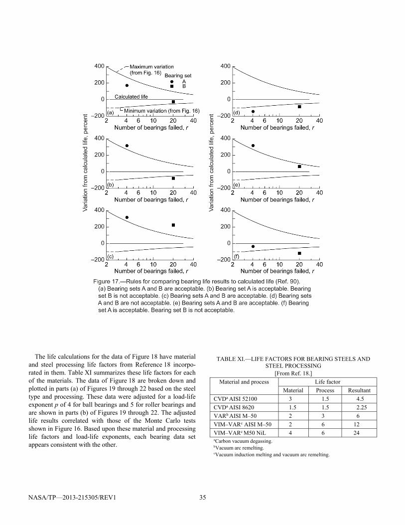
NASA/TP—2013-215305/REV1 35

The life calculations for the data of Figure 18 have material and steel processing life factors from Reference 18 incorpo-rated in them. Table XI summarizes these life factors for each of the materials. The data of Figure 18 are broken down and plotted in parts (a) of Figures 19 through 22 based on the steel type and processing. These data were adjusted for a load-life exponent p of 4 for ball bearings and 5 for roller bearings and are shown in parts (b) of Figures 19 through 22. The adjusted life results correlated with those of the Monte Carlo tests shown in Figure 16. Based upon these material and processing life factors and load-life exponents, each bearing data set appears consistent with the other.

TABLE XI.—LIFE FACTORS FOR BEARING STEELS AND STEEL PROCESSING

[From Ref. 18.]

Material and process Life factor

Material Process Resultant

CVDa AISI 52100 3 1.5 4.5

CVDa AISI 8620 1.5 1.5 2.25

VARb AISI M–50 2 3 6

VIM–VARc AISI M–50 2 6 12

VIM–VARc M50 NiL 4 6 24 aCarbon vacuum degassing. bVacuum arc remelting. cVacuum induction melting and vacuum arc remelting.

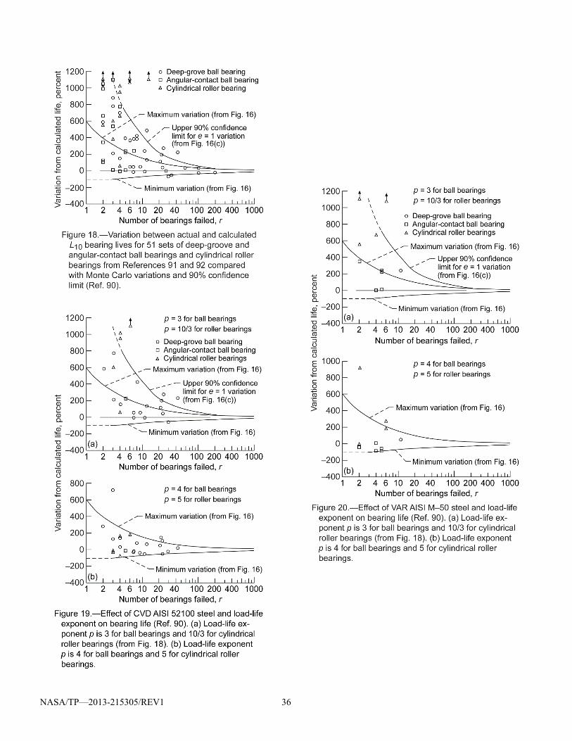
NASA/TP—2013-215305/REV1 36

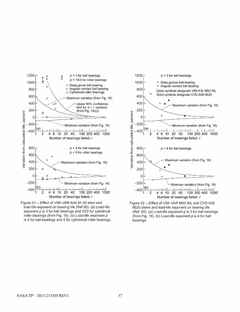
NASA/TP—2013-215305/REV1 37

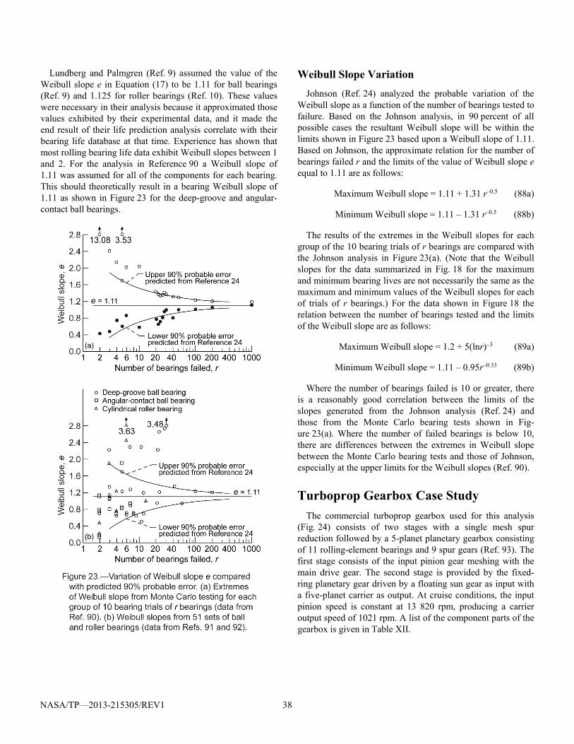
NASA/TP—2013-215305/REV1 38

Lundberg and Palmgren (Ref. 9) assumed the value of the Weibull slope e in Equation (17) to be 1.11 for ball bearings (Ref. 9) and 1.125 for roller bearings (Ref. 10). These values were necessary in their analysis because it approximated those values exhibited by their experimental data, and it made the end result of their life prediction analysis correlate with their bearing life database at that time. Experience has shown that most rolling bearing life data exhibit Weibull slopes between 1 and 2. For the analysis in Reference 90 a Weibull slope of 1.11 was assumed for all of the components for each bearing. This should theoretically result in a bearing Weibull slope of 1.11 as shown in Figure 23 for the deep-groove and angular-contact ball bearings.

Weibull Slope Variation

Johnson (Ref. 24) analyzed the probable variation of the Weibull slope as a function of the number of bearings tested to failure. Based on the Johnson analysis, in 90 percent of all possible cases the resultant Weibull slope will be within the limits shown in Figure 23 based upon a Weibull slope of 1.11. Based on Johnson, the approximate relation for the number of bearings failed r and the limits of the value of Weibull slope e equal to 1.11 are as follows:

Maximum Weibull slope = 1.11 + 1.31 r–0.5 (88a)

Minimum Weibull slope = 1.11 – 1.31 r–0.5 (88b)

The results of the extremes in the Weibull slopes for each group of the 10 bearing trials of r bearings are compared with the Johnson analysis in Figure 23(a). (Note that the Weibull slopes for the data summarized in Fig. 18 for the maximum and minimum bearing lives are not necessarily the same as the maximum and minimum values of the Weibull slopes for each of trials of r bearings.) For the data shown in Figure 18 the relation between the number of bearings tested and the limits of the Weibull slope are as follows:

Maximum Weibull slope = 1.2 + 5(lnr)–3 (89a)

Minimum Weibull slope = 1.11 – 0.95r–0.33 (89b)

Where the number of bearings failed is 10 or greater, there is a reasonably good correlation between the limits of the slopes generated from the Johnson analysis (Ref. 24) and those from the Monte Carlo bearing tests shown in Fig-ure 23(a). Where the number of failed bearings is below 10, there are differences between the extremes in Weibull slope between the Monte Carlo bearing tests and those of Johnson, especially at the upper limits for the Weibull slopes (Ref. 90).

Turboprop Gearbox Case Study

The commercial turboprop gearbox used for this analysis (Fig. 24) consists of two stages with a single mesh spur reduction followed by a 5-planet planetary gearbox consisting of 11 rolling-element bearings and 9 spur gears (Ref. 93). The first stage consists of the input pinion gear meshing with the main drive gear. The second stage is provided by the fixed-ring planetary gear driven by a floating sun gear as input with a five-planet carrier as output. At cruise conditions, the input pinion speed is constant at 13 820 rpm, producing a carrier output speed of 1021 rpm. A list of the component parts of the gearbox is given in Table XII.

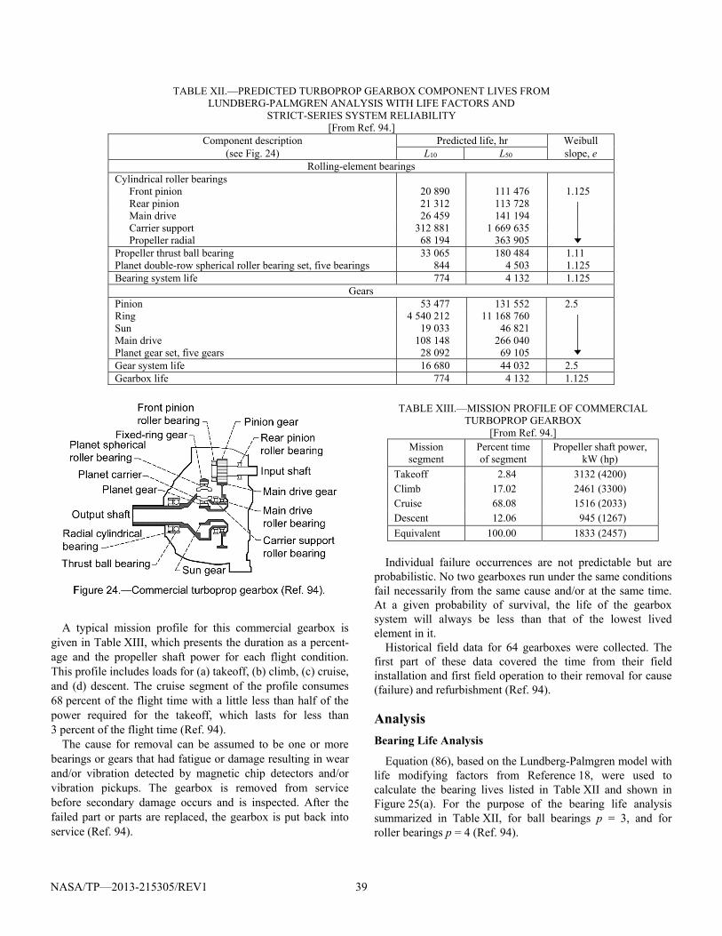
NASA/TP—2013-215305/REV1 39

TABLE XII.—PREDICTED TURBOPROP GEARBOX COMPONENT LIVES FROM LUNDBERG-PALMGREN ANALYSIS WITH LIFE FACTORS AND

STRICT-SERIES SYSTEM RELIABILITY [From Ref. 94.]

Component description Predicted life, hr Weibull (see Fig. 24) L10 L50 slope, e

Rolling-element bearings Cylindrical roller bearings Front pinion 20 890 111 476 1.125 Rear pinion 21 312 113 728

Main drive 26 459 141 194 Carrier support 312 881 1 669 635 Propeller radial 68 194 363 905 Propeller thrust ball bearing 33 065 180 484 1.11 Planet double-row spherical roller bearing set, five bearings 844 4 503 1.125 Bearing system life 774 4 132 1.125

Gears Pinion 53 477 131 552 2.5 Ring 4 540 212 11 168 760 Sun 19 033 46 821 Main drive 108 148 266 040 Planet gear set, five gears 28 092 69 105 Gear system life 16 680 44 032 2.5 Gearbox life 774 4 132 1.125

A typical mission profile for this commercial gearbox is

given in Table XIII, which presents the duration as a percent-age and the propeller shaft power for each flight condition. This profile includes loads for (a) takeoff, (b) climb, (c) cruise, and (d) descent. The cruise segment of the profile consumes 68 percent of the flight time with a little less than half of the power required for the takeoff, which lasts for less than 3 percent of the flight time (Ref. 94).

The cause for removal can be assumed to be one or more bearings or gears that had fatigue or damage resulting in wear and/or vibration detected by magnetic chip detectors and/or vibration pickups. The gearbox is removed from service before secondary damage occurs and is inspected. After the failed part or parts are replaced, the gearbox is put back into service (Ref. 94).

TABLE XIII.—MISSION PROFILE OF COMMERCIAL TURBOPROP GEARBOX

[From Ref. 94.] Mission segment

Percent time of segment

Propeller shaft power, kW (hp)

Takeoff 2.84 3132 (4200) Climb 17.02 2461 (3300) Cruise 68.08 1516 (2033) Descent 12.06 945 (1267)

Equivalent 100.00 1833 (2457)

Individual failure occurrences are not predictable but are

probabilistic. No two gearboxes run under the same conditions fail necessarily from the same cause and/or at the same time. At a given probability of survival, the life of the gearbox system will always be less than that of the lowest lived element in it.

Historical field data for 64 gearboxes were collected. The first part of these data covered the time from their field installation and first field operation to their removal for cause (failure) and refurbishment (Ref. 94).

Analysis

Bearing Life Analysis

Equation (86), based on the Lundberg-Palmgren model with life modifying factors from Reference 18, were used to calculate the bearing lives listed in Table XII and shown in Figure 25(a). For the purpose of the bearing life analysis summarized in Table XII, for ball bearings p = 3, and for roller bearings p = 4 (Ref. 94).

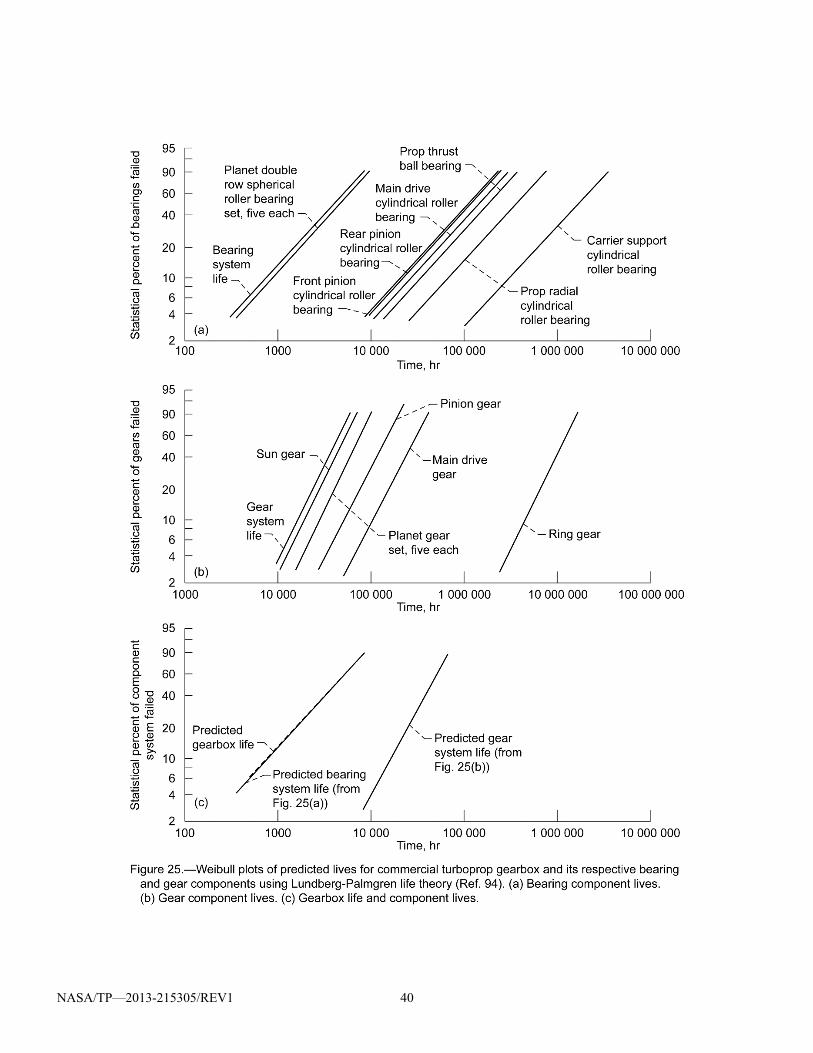
NASA/TP—2013-215305/REV1 40

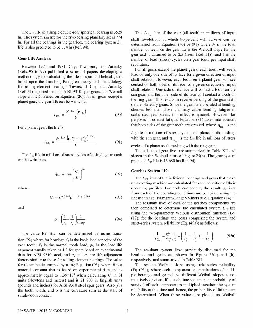
NASA/TP—2013-215305/REV1 41

The L10 life of a single double-row spherical bearing is 3529 hr. The system L10 life for the five-bearing planetary set is 774 hr. For all the bearings in the gearbox, the bearing system L10 life is also predicted to be 774 hr (Ref. 94).

Gear Life Analysis

Between 1975 and 1981, Coy, Townsend, and Zaretsky (Refs. 95 to 97) published a series of papers developing a methodology for calculating the life of spur and helical gears based upon the Lundberg-Palmgren theory and methodology for rolling-element bearings. Townsend, Coy, and Zaretsky (Ref. 51) reported that for AISI 9310 spur gears, the Weibull slope e is 2.5. Based on Equation (20), for all gears except a planet gear, the gear life can be written as

k

NL t

G

G

e10

/1

10

(90)

For a planet gear, the life is

k

NL

GG

t

G

tG

G

eeee/1

1010/1

1021

(91)

The L10 life in millions of stress cycles of a single gear tooth can be written as

G

t

p

t

t

P

Caa

3210 (92)

where

093.0165.1907.0 lBfCt (93)

and

sin

111

21 rr (94)

The value for t10 can be determined by using Equa-

tion (92) where for bearings Ct is the basic load capacity of the gear tooth, Pt is the normal tooth load, pG is the load-life exponent usually taken as 4.3 for gears based on experimental data for AISI 9310 steel, and a2 and a3 are life adjustment factors similar to those for rolling-element bearings. The value for Ct can be determined by using Equation (93), where B is a material constant that is based on experimental data and is approximately equal to 1.39108 when calculating Ct in SI units (Newtons and meters) and is 21 800 in English units (pounds and inches) for AISI 9310 steel spur gears. Also, f is the tooth width, and ρ is the curvature sum at the start of single-tooth contact.

The G

L10 life of the gear (all teeth) in millions of input

shaft revolutions at which 90 percent will survive can be determined from Equation (90) or (91) where N is the total number of teeth on the gear, eG is the Weibull slope for the gear and is assumed to be 2.5 (from (Ref. 51)), and k is the number of load (stress) cycles on a gear tooth per input shaft revolution.

For all gears except the planet gears, each tooth will see a load on only one side of its face for a given direction of input shaft rotation. However, each tooth on a planet gear will see contact on both sides of its face for a given direction of input shaft rotation. One side of its face will contact a tooth on the sun gear, and the other side of its face will contact a tooth on the ring gear. This results in reverse bending of the gear teeth on the planetary gears. Since the gears are operated at bending stresses less than those that may cause bending fatigue in carburized gear steels, this effect is ignored. However, for purposes of contact fatigue, Equation (91) takes into account that both sides of the gear tooth are stressed, where

110η

t

is the

L10 life in millions of stress cycles of a planet tooth meshing with the sun gear, and

210η

t

is the L10 life in millions of stress

cycles of a planet tooth meshing with the ring gear. The calculated gear lives are summarized in Table XII and

shown in the Weibull plots of Figure 25(b). The gear system predicted L10 life is 16 680 hr (Ref. 94).

Gearbox System Life

The L10 lives of the individual bearings and gears that make up a rotating machine are calculated for each condition of their operating profiles. For each component, the resulting lives from each of the operating conditions are combined using the linear damage (Palmgren-Langer-Miner) rule, Equation (14).

The resultant lives of each of the gearbox components are then combined to determine the calculated system L10 life using the two-parameter Weibull distribution function (Eq. (17)) for the bearings and gears comprising the system and strict-series system reliability (Eq. (49a)) as follows:

n

ien

eeen

esys LLLLL 1 21

1...

1111 (95a)

The resultant system lives previously discussed for the bearings and gears are shown in Figures 25(a) and (b), respectively, and summarized in Table XII.

The system Weibull slope using strict-series reliability (Eq. (95a)) where each component or combinations of multi-ple bearings and gears have different Weibull slopes is not intuitively obvious. If at each time sequence the probability of survival of each component is multiplied together, the system reliability at that time and, hence, the probability of failure can be determined. When these values are plotted on Weibull

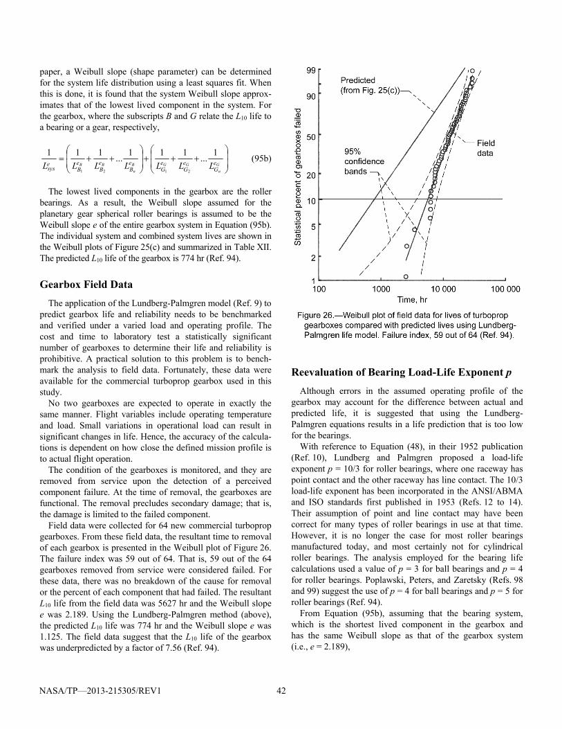
NASA/TP—2013-215305/REV1 42

paper, a Weibull slope (shape parameter) can be determined for the system life distribution using a least squares fit. When this is done, it is found that the system Weibull slope approx-imates that of the lowest lived component in the system. For the gearbox, where the subscripts B and G relate the L10 life to a bearing or a gear, respectively,

G

n

GGB

n

BB eG

eG

eG

eB

eB

eB

esys LLLLLLL

1...

111...

111

2121

(95b)

The lowest lived components in the gearbox are the roller bearings. As a result, the Weibull slope assumed for the planetary gear spherical roller bearings is assumed to be the Weibull slope e of the entire gearbox system in Equation (95b). The individual system and combined system lives are shown in the Weibull plots of Figure 25(c) and summarized in Table XII. The predicted L10 life of the gearbox is 774 hr (Ref. 94).

Gearbox Field Data

The application of the Lundberg-Palmgren model (Ref. 9) to predict gearbox life and reliability needs to be benchmarked and verified under a varied load and operating profile. The cost and time to laboratory test a statistically significant number of gearboxes to determine their life and reliability is prohibitive. A practical solution to this problem is to bench-mark the analysis to field data. Fortunately, these data were available for the commercial turboprop gearbox used in this study.

No two gearboxes are expected to operate in exactly the same manner. Flight variables include operating temperature and load. Small variations in operational load can result in significant changes in life. Hence, the accuracy of the calcula-tions is dependent on how close the defined mission profile is to actual flight operation.

The condition of the gearboxes is monitored, and they are removed from service upon the detection of a perceived component failure. At the time of removal, the gearboxes are functional. The removal precludes secondary damage; that is, the damage is limited to the failed component.

Field data were collected for 64 new commercial turboprop gearboxes. From these field data, the resultant time to removal of each gearbox is presented in the Weibull plot of Figure 26. The failure index was 59 out of 64. That is, 59 out of the 64 gearboxes removed from service were considered failed. For these data, there was no breakdown of the cause for removal or the percent of each component that had failed. The resultant L10 life from the field data was 5627 hr and the Weibull slope e was 2.189. Using the Lundberg-Palmgren method (above), the predicted L10 life was 774 hr and the Weibull slope e was 1.125. The field data suggest that the L10 life of the gearbox was underpredicted by a factor of 7.56 (Ref. 94).

Reevaluation of Bearing Load-Life Exponent p

Although errors in the assumed operating profile of the gearbox may account for the difference between actual and predicted life, it is suggested that using the Lundberg-Palmgren equations results in a life prediction that is too low for the bearings.

With reference to Equation (48), in their 1952 publication (Ref. 10), Lundberg and Palmgren proposed a load-life exponent p = 10/3 for roller bearings, where one raceway has point contact and the other raceway has line contact. The 10/3 load-life exponent has been incorporated in the ANSI/ABMA and ISO standards first published in 1953 (Refs. 12 to 14). Their assumption of point and line contact may have been correct for many types of roller bearings in use at that time. However, it is no longer the case for most roller bearings manufactured today, and most certainly not for cylindrical roller bearings. The analysis employed for the bearing life calculations used a value of p = 3 for ball bearings and p = 4 for roller bearings. Poplawski, Peters, and Zaretsky (Refs. 98 and 99) suggest the use of p = 4 for ball bearings and p = 5 for roller bearings (Ref. 94).

From Equation (95b), assuming that the bearing system, which is the shortest lived component in the gearbox and has the same Weibull slope as that of the gearbox system (i.e., e = 2.189),

NASA/TP—2013-215305/REV1 43

GBs e

GeB

esys LLL

111 (96a)

and substituting in the known values

5.2189.2189.2 680,16

11

5627

1

BL (96b)

and solving for the bearing system life, results in a value of

hr5627BL (96c)

From Lundberg-Palmgren (Ref. 9), the predicted bearing system life is

hr774~~

4

eq

DB

P

CL (97a)

then,

27.5~

eq

D

P

C (97b)

Calculating a revised value for the load-life exponent p for the gearbox bearings based on the actual bearing system life of 5627 hr,

hr5627~27.5~ p

p

eq

D

P

C

(98a)

Solving for load-life exponent p,

2.5p (98b)

Referring to Equation (43c), for line contact (roller bearing) the Hertz stress-life exponent n = 2p. From Equation (98b), n = 10.4 for line contact for the turboprop gearbox data.

Referring to the Zaretsky model for line contact, Equation (62b), the shear stress-life exponent is

e

nc1

(99a)

and where n = 10.4 and e = 2.189,

943.9189.2

14.10 c (99b)

Using the value of c from Equation (99b) in Equation (62a) for point contact where e is assumed to equal 1.11, then

74.1111.1

2943.9

2

ecn (100a)

and for point contact,

91.33

74.11

3

np (100b)

The apparent load-life exponent p for the roller bearings is equal to 5.2 and correlates with the Zaretsky model. Were the roller bearing lives to be recalculated using a load-life exponent p = 5.2, the predicted L10 life of the gearbox would be equal to the actual life obtained in the field, 5627 hr. It should be noted that if an exponent p = 5 were used, the predicted L10 life of the gearbox would be 4065 hr. This result suggests a strong reliance of the predicted bearing life upon the load-life exponent p. The values of the load-life exponent p for roller bearings equal to 10/3 from the ANSI/ABMA and ISO standards (Refs. 12 and 14) and 4 from computer codes may provide predicted roller bearing lives that are too conservative for design purposes. The use of the ANSI/ABMA and ISO standards load-life exponent of 10/3 to predict roller bearing life is not reflective of modern roller bearings. It will underpredict bearing lives.

Glenn Research Center National Aeronautics and Space Administration Cleveland, Ohio, March 6, 2013

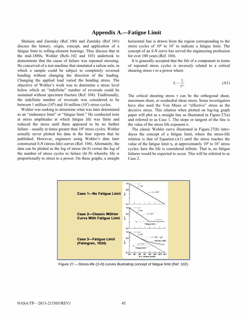
NASA/TP—2013-215305/REV1 45

Appendix A.—Fatigue Limit Shimizu and Zaretsky (Ref. 100) and Zaretsky (Ref. 101)

discuss the history, origin, concept, and application of a fatigue limit to rolling-element bearings. They discuss that in the mid-1880s, Wohler (Refs. 102 and 103) undertook to demonstrate that the cause of failure was repeated stressing. He conceived of a test machine that simulated a railcar axle, in which a sample could be subject to completely reversed bending without changing the direction of the loading. Changing the applied load varied the bending stress. The objective of Wohler’s work was to determine a stress level below which an “indefinite” number of reversals could be sustained without specimen fracture (Ref. 104). Traditionally, the indefinite number of reversals was considered to be between 1 million (106) and 10 million (107) stress cycles.

Wohler was seeking to determine what was later determined as an “endurance limit” or “fatigue limit.” He conducted tests at stress amplitudes at which fatigue life was finite and reduced the stress until there appeared to be no further failure—usually at times greater than 106 stress cycles. Wohler actually never plotted his data in the four reports that he published. However, engineers using Wohler’s data later constructed S-N (stress-life) curves (Ref. 104). Alternately, the data can be plotted as the log of stress (ln S) versus the log of the number of stress cycles to failure (ln N) whereby life is proportionally to stress to a power. On these graphs, a straight

horizontal line is drawn from the region corresponding to the stress cycles of 106 to 107 to indicate a fatigue limit. The concept of an S-N curve has served the engineering profession for over 100 years (Ref. 104).

It is generally accepted that the life of a component in terms of repeated stress cycles is inversely related to a critical shearing stress τ to a power where

n

L1

~ (A1)

The critical shearing stress τ can be the orthogonal shear, maximum shear, or octahedral shear stress. Some investigators have also used the Von Mises or “effective” stress as the decisive stress. This relation when plotted on log-log graph paper will plot as a straight line as illustrated in Figure 27(a) and referred to as Case 1. The slope or tangent of the line is the value of the stress life exponent n.

The classic Wohler curve illustrated in Figure 27(b) intro-duces the concept of a fatigue limit, where the stress-life relation is that of Equation (A1) until the stress reaches the value of the fatigue limit τf, at approximately 106 to 107 stress cycles; here the life is considered infinite. That is, no fatigue failures would be expected to occur. This will be referred to as Case 2.

Figure 27.—Stress-life (S-N) curves illustrating concept of fatigue limit (Ref. 102).

NASA/TP—2013-215305/REV1 46

In practice, fatigue data for material types that have fatigue limits do not manifest a linear line on a log-log S-N plot, but a curved line as illustrated in Figure 27(c). This will be referred to as Case 3. The apparent relation between life, shearing stress τ, and fatigue limit τf is

nf

L1

~ (A2)

For an applied stress and the presence of a fatigue limit, the resultant life from Equation (A2) will be longer than that from Equation (A1) with a fatigue limit (Refs. 100 and 101).

Allan (Ref. 105) discusses the contributions of Goodman to rolling bearing technology. Goodman (Refs. 2 and 106) derived for thrust and radial ball bearings and the cylindrical roller bearing empirical formulae for “safe loads” at or below which no failure should occur (Refs. 105 and 107). Goodman’s experiments began in 1896 (Ref. 105). He experimentally adopted an approach for rolling-element bearings similar to that of Wohler for rotating beam fatigue. Bearing endurance tests were conducted under varying loads. He categorized his testing into low-speed bearings and high-speed bearings. Although Goodman was familiar with Hertzi-an theory, he plotted the results in terms of load versus life in total shaft revolutions (inner-race revolutions) and curve-fit the data (Ref. 105). Where Wohler defined life in terms of stress cycles, Goodman defined a “safe load” for “low-speed” bearings at a life of 1 million shaft (inner-race) revolutions where no failure has occurred and “several million” shaft (inner-race) revolutions for high-speed bearings (Ref. 105). The failure mode as defined by Goodman could be any damage to the ball surface of a ball bearing and not just that caused by fatigue. For bearing running times (life) equal to or greater than 106 shaft (inner-race) revolutions without failure (damage), Goodman’s empirical formulae for “safe loads” are as follows (Ref. 107):

Thrust bearings, grooved races:

Thrust load dNR

Zd

ii 2002

0002501 3

lb (A3)

Radial bearings, grooved races:

Radial load dNR

Zd

ii 20002

0000002 3

lb (A4)

Cylindrical roller bearings, radially loaded:

Radial load dNR

KZld

ii 20002

2

lb (A5)

where Z number of balls or rollers d ball or roller diameter, in. Ri effective radius of inner ring, in.

Ni speed of inner ring, rpm K constant of 1 200 000 to 2 000 000 l length of rollers, in.

Although the above loads are not a “fatigue limit” per se, they can be considered an “endurance limit” that reflected rolling bearing state of the art in the United Kingdom at the turn of the 20th century.

In 1924 Palmgren (Ref. 4) published an empirical formula based on the concept of an L10 life, or the time that 90 percent of a bearing population would equal or exceed without rolling-element fatigue failure. This paper by Palmgren represents the first time in the literature that a probabilistic approach to life prediction of a machine element was formulated. Assuming that a ball or roller bearing was properly designed, manufac-tured, installed, lubricated, and maintained, rolling-element fatigue would limit the useable life of the bearing. In the life equations that Palmgren presented he incorporated a “fatigue limit,” or load below which no failure will occur, as well as a time or “location parameter” before which time no failure should occur (Ref. 20). The Palmgren form (Ref. 4) of the “fatigue limit” takes the form of Case 3, but, as with Good-man, it uses load and not stress. Although Palmgren does not reference either Wohler or Goodman, it is not unreasonable to assume that the inclusion of a fatigue limit in his life equation (see Eq. (5)) was influenced by their respective works.

In 1936 Palmgren (Ref. 33) abandoned the concept of a fatigue limit for rolling-element bearings. The concept of a fatigue limit does not appear in his 1945 book (Ref. 5) nor is it included in the Lundberg-Palmgren life theory (Refs. 9 and 10). In 1985 Ioannides and Harris (Ref. 32) applied Palmgren’s 1924 concept of a “fatigue limit” (Eq. (A3), Case 3, Fig. 27(c)) to the 1947 Lundberg-Palmgren equations (Ref. 9) (see Eqs. (54) to (55)). However, there is no database for rolling-element bearings or for conventional fatigue specimens that supports the existence of a fatigue limit for through-hardened bearing steels or, more specifically, through-hardened AISI 52100 bearing steel.

A leader in the effort to determine if a fatigue limit exists for AISI 52100 steel is Professor Shigeo Shimizu (Ref. 100) of the School of Science and Technology, Meiji University, Kawasaki, Kanagawa, Japan. He reasoned that a material when tested should only react to its state of stress and envi-ronment. That is, if AISI 52100 steel had a fatigue limit, a stress below which no failure will occur, it should exhibit this “fatigue limit” no matter what type of fatigue test was per-formed. A statistically significant number of fatigue tests are required over a range of shearing stresses to assure with reasonable engineering and scientific certainty that the steel either did or did not exhibit a fatigue limit; also, if a fatigue limit did exist, what its value was (Ref. 101).

NASA/TP—2013-215305/REV1 47

In 2008, Shimizu together with his colleagues, Professors K. Tosha, D. Ueda, and H. Shimoda published a journal paper in STLE Tribology Transactions reporting the results of rotating beam fatigue experiments for through-hardened AISI 52100 steel at very low shearing stresses as low as 0.48 GPA (69.6 ksi) (Ref. 35). “The test results produced fatigue lives in excess of 100 million stress cycles without the manifestation of a fatigue limit.”

In order to assure the credibility of his work, additional re-search was conducted and published by Shimizu together with his colleagues, Professors K. Tsuchiya, and K. Tosha in the 2009 STLE Tribology Transactions (Ref. 36). They tested six groups of AISI 52100 bearing steel specimens using four-alternating torsion fatigue life test rigs to determine whether a fatigue limit exists or not and to compare the resultant shear stress-life relation with that used for rolling-element bearing life prediction.

The number of specimens in each sample size ranged from 19 to 33 specimens for a total of 150 tests. The tests were run at 0.5, 0.63, 0.76, 0.80, 0.95, and 1.00 GPa (75.5, 91.4, 110.2, 116.0, 137.8, and 145 ksi) maximum shearing stress ampli-tudes. The stress-life curves of these data shown in Figure 28 show an inverse dependence of life on the shearing stress as in Case 1 (Fig. 27(a)), but do not show an inverse relation on the difference of the shearing stress minus a fatigue limiting stress as in Case 3 (Fig. 27(c)). The shear stress-life exponent n for the AISI 52100 steel was 10.34 from the three-parameter Weibull analysis and was independent of the Weibull slope e (Ref. 36). This compares with a shear stress-life exponent of 9.3 from Lundberg and Palmgren (Ref. 9). From these tests, it can be concluded with reasonable engineering and statistical certainty that a “fatigue limit” does not exist for through-hardened AISI 52100 bearing steel (Refs. 100 and 101).

NASA/TP—2013-215305/REV1 49

Appendix B.—Derivation of Weibull Distribution Function

According to Weibull (Refs. 6 and 7) and as presented in Reference 108 (see also Ref. 98), any distribution function can be written as

XXF fexp1 (B1)

where F(X) is the probability of an event (failure) occurring and f(X) is a function of an operating variable X. Conversely, from Equation (B1) the probability of an event not occurring (survival) can be written as

XXF fexp1 (B2a)

or

XF fexp1 (B2b)

where F = F(X) and (1 – F) = S, the probability of survival. If there are n independent components, each with a proba-

bility of the event (failure) not occurring (1 – F), the probabil-ity of the event not occurring in the combined total of all components can be expressed from Equation (B2b) as

XnF n fexp1 (B3)

Equation (B3) gives the appropriate mathematical expres-sion for the principle of the weakest link in a chain or, more generally, for the size effect on failures in solids. The applica-tion of Equation (B3) is illustrated by a chain consisting of several links. Testing finds the probability of failure F at any load X applied to a “single” link. To find the probability of failure Fn of a chain consisting of n links, one must assume that if one link has failed the whole chain fails. That is, if any single part of a component fails, the whole component has failed. Accordingly, the probability of nonfailure of the chain (1–Fn), is equal to the probability of the simultaneous nonfail-ure of all the links. Thus,

nn FF 11 (B4a)

or

n

n SS (B4b)

where the probabilities of failure (or survival) of each link are not necessarily equal (i.e., S1 S2 S3 …), Equation (B4b) can be expressed as

...321 SSSSn (B4c)

This is the same as Equation (18) of the main text. From equation (B3) for a uniform distribution of stresses

throughout a volume V,

fexp1 VFv (B5a)

or

fexp1 VFS v (B5b)

Equation (B5b) can be expressed as follows:

VS

lnfln1

lnln

(B6)

It follows that if ln ln (1/S) is plotted as the ordinate and ln

f() as the abscissa in a system of rectangular coordinates, a variation of volume V of the test specimen will imply only a parallel displacement but no deformation of the distribution function. Weibull (Ref. 6) assumed the form

e

u

u

f (B7)

where e is the Weibull slope, is a stress at a given probabil-ity of failure, u is a location parameter below which stress no failure will occur, and is the characteristic stress at which 63.2 percent of the population will fail. Equation (B6) be-comes

VeeS

uu lnlnln1

lnln

(B8)

If the location parameter u is assumed to be zero, and V is normalized whereby ln V is zero, equation (A8) can be written as

ln1

lnln eS

where 0 < < and 0 < S < 1 (B9)

Equation (B9) is identical to Equation (17) of the main text. The form of equation (B9), where u in Equation (B8) is

assumed to be zero, is referred to as “two-parameter Weibull.” Where u is not assumed to be zero, the form of the equation is referred to as “three-parameter Weibull.”

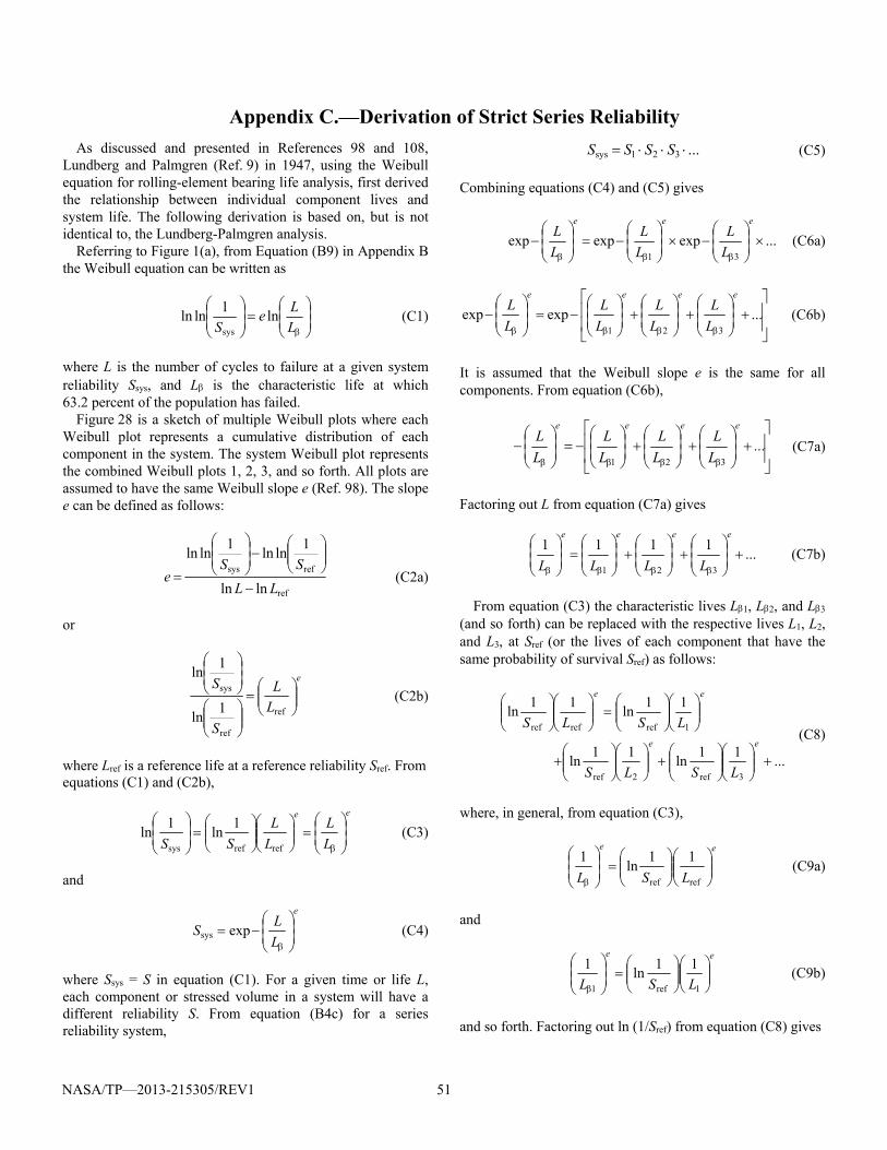
NASA/TP—2013-215305/REV1 51

Appendix C.—Derivation of Strict Series Reliability

As discussed and presented in References 98 and 108, Lundberg and Palmgren (Ref. 9) in 1947, using the Weibull equation for rolling-element bearing life analysis, first derived the relationship between individual component lives and system life. The following derivation is based on, but is not identical to, the Lundberg-Palmgren analysis.

Referring to Figure 1(a), from Equation (B9) in Appendix B the Weibull equation can be written as

L

Le

Sln

1lnln

sys

(C1)

where L is the number of cycles to failure at a given system reliability Ssys, and L is the characteristic life at which 63.2 percent of the population has failed.

Figure 28 is a sketch of multiple Weibull plots where each Weibull plot represents a cumulative distribution of each component in the system. The system Weibull plot represents the combined Weibull plots 1, 2, 3, and so forth. All plots are assumed to have the same Weibull slope e (Ref. 98). The slope e can be defined as follows:

ref

refsys

lnln

1lnln

1lnln

LL

SSe

(C2a)

or

e

L

L

S

S

ref

ref

sys

1ln

1ln

(C2b)

where Lref is a reference life at a reference reliability Sref. From equations (C1) and (C2b),

ee

L

L

L

L

SS

refrefsys

1ln

1ln (C3)

and

e

L

LS

expsys (C4)

where Ssys = S in equation (C1). For a given time or life L, each component or stressed volume in a system will have a different reliability S. From equation (B4c) for a series reliability system,

...321sys SSSS (C5)

Combining equations (C4) and (C5) gives

...expexpexp31

eee

L

L

L

L

L

L (C6a)

...expexp321

eeee

L

L

L

L

L

L

L

L (C6b)

It is assumed that the Weibull slope e is the same for all components. From equation (C6b),

...

L

L

L

L

L

L

L

Leeee

3β2β1ββ

(C7a)

Factoring out L from equation (C7a) gives

...1111

321

eeee

LLLL (C7b)

From equation (C3) the characteristic lives L1, L2, and L3 (and so forth) can be replaced with the respective lives L1, L2, and L3, at Sref (or the lives of each component that have the same probability of survival Sref) as follows:

...

11ln

11ln

11ln

11ln

3ref2ref

1refrefref

ee

ee

LSLS

LSLS (C8)

where, in general, from equation (C3),

ee

LSL

refref

11ln

1 (C9a)

and

ee

LSL

1ref1

11ln

1 (C9b)

and so forth. Factoring out ln (1/Sref) from equation (C8) gives

NASA/TP—2013-215305/REV1 52

eeee

LLLL

/1

321ref

...1111

(C10)

or rewriting equation (C10) results in

n

i

e

i

e

LL 1

11 (C11)

Equation (C11) is identical to Equations (47) and (49a) of the text.

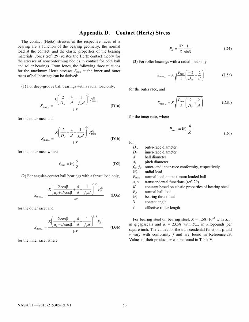
NASA/TP—2013-215305/REV1 53

Appendix D.—Contact (Hertz) Stress

The contact (Hertz) stresses at the respective races of a bearing are a function of the bearing geometry, the normal load at the contact, and the elastic properties of the bearing materials. Jones (ref. 29) relates the Hertz contact theory for the stresses of nonconforming bodies in contact for both ball and roller bearings. From Jones, the following three relations for the maximum Hertz stresses Smax at the inner and outer races of ball bearings can be derived:

(1) For deep-groove ball bearings with a radial load only,

v

PdfdD

K

S ororor

31

32

max

max

142

(D1a)

for the outer race, and

v

PdfdD

K

S iririr

31

32

max

max

142

(D1b)

for the inner race, where

Z

WP r5

max (D2)

(2) For angular-contact ball bearings with a thrust load only,

v

Pdfddd

K

SN

oreor

31

3/2

max

14

cos

cos2

(D3a)

for the outer race, and

v

Pdfddd

K

SN

ireir

31

3/2

max

14

cos

cos2

(D3b)

for the inner race, where

sin

1

Z

WtPN (D4)

(3) For roller bearings with a radial load only

dD

PKS

oror

22maxmax

(D5a)

for the outer race, and

dD

PKS

irir

22maxmax

(D5b)

for the inner race, where

ZWP r

4max

(D6)

for Dor outer-race diameter Dir inner-race diameter d ball diameter de pitch diameter for, fir outer- and inner-race conformity, respectively Wr radial load Pmax normal load on maximum loaded ball , v transcendental functions (ref. 29) K constant based on elastic properties of bearing steel PN normal ball load Wt bearing thrust load contact angle

effective roller length

For bearing steel on bearing steel, K = 1.5810–3 with Smax

in gigapascals and K = 23.58 with Smax in kilopounds per square inch. The values for the transcendental functions and v vary with conformity f and are found in Reference 29. Values of their product v can be found in Table V.

NASA/TP—2013-215305/REV1 54

References

1. Stribeck, R.: Reports From the Central Laboratory for Scientific Investigation. Translation by H. Hess, ASME Trans., vol. 29, 1907, pp. 420–466.

2. Goodman, J.: Roller and Ball Bearings. Minutes of the Proceedings of the Institution of Civil Engineers, vol. 189, pt. 3, 1912, pp. 82–127.

3. Colvin, Fred H.; and Stanley, Frank A.: American Ma-chinists’ Handbook and Dictionary of Shop Terms; A Reference Book of Machine Shop and Drawing Room Data, Methods and Definitions. Second ed., McGraw-Hill, New York, NY, 1914, pp. 381–386.

4. Palmgren, A.: The Service Life of Ball Bearings. Z. Ver. Deut. Ingr. (NASA TT F–13460), vol. 68, no. 14, 1924, pp. 339–341.

5. Palmgren, Arvid: Ball and Roller Bearing Engineering. Translation by Gunnar Palmgren and Bryce Ruley, SKF Industries, Philadelphia, PA, 1945.

6. Weibull, W.: A Statistical Theory of the Strength of Materials. Inginioersvetenskapsakad. Handl. (Proc. Royal Swedish Academy of Engr.), no. 151, 1939.

7. Weibull, W.: The Phenomenon of Rupture in Solids. Inginioersvetenskapsakad. Handl. (Proc. Royal Swedish Academy of Engr.), no. 153, 1939.

8. Thomas, Howard R.; and Hoersch, Victor A.: Stresses Due to the Pressure of One Elastic Solid Upon Another With Special Reference to Railroad Rails. Bulletin No. 212, University of Illinois Engineering Experiment Sta-tion, Urbana, IL, 1930.

9. Lundberg, G.; and Palmgren, A.: Dynamic Capacity of Rolling Bearings. Acta Polytech. Mech. Eng. Ser., vol. 1, no. 3, 1947.

10. Lundberg, G.; and Palmgren, A.: Dynamic Capacity of Roller Bearings. Inginioersvetenskapsakad. Handl. no. 210, The Royal Swedish Academy of Engineering Science, Stockholm, Sweden, 1952.

11. Hertz, Heinrich: Uber die Beruehrung elasticher Koerper (On Contact of Elastic Bodies). Gesammelte Werke (Collected Works), Vol. 1, Leipzig, Germany, 1881.

12. ISO 281: Rolling Bearings—Dynamic Load Ratings and Rating Life. International Organization for Stand-ards, Geneva, 1990.

13. ABMA 9: Load Ratings and Fatigue Life for Ball Bear-ings. American Bearing Manufacturers Association, Washington, DC, 1990.

14. ABMA 11: Load Ratings and Fatigue Life for Roller Bearings. American Bearing Manufacturers Associa-tion, Washington, DC, 1990.

15. Zaretsky, Erwin V., ed.: Tribology for Aerospace Ap-plications. STLE SP–37, Society of Triboligists and Lubrication Engineers, Park Ridge, IL, 1997.

16. Ertel, A.M.: Hydrodynamic Lubrication Based on New Principles. Prikadnaya Matematika I Mechanika (in Russian), vol. 3, no. 2, 1939.

17. Grubin, A.N.; and Vinogradova, E.: Fundamentals of the Hydrodynamic Theory of Lubrication of Heavily Loaded Cylindrical Surfaces. Investigation of the Con-tact of Machine Components. Kh. F. Ketova, ed., trans-lation of Russian Book No. 30, Central Scientific Research Institute for Technology and Mechanical En-gineering, Moscow (Available from Dept. of Scientific and Industrial Research, Great Britain, Trans. CTS–235, and from Special Libraries Association, Chicago Transl. R–3554.), 1949.

18. Zaretsky, Erwin V., ed.: STLE Life Factors for Rolling Bearings. STLE SP–34, Society of Triboligists and Lu-brication Engineers, Park Ridge, IL 1992.

19. Styri, H.: Investigations of Rolling Bearings at SKF In-dustries, Inc. Review of Current and Anticipated Lubri-cant Problems in Turbojet Engines, NACA RM 51D20, 1951, pp. 30–39.

20. Zaretsky. Erwin V.: A Palmgren Revisited—A Basis for Bearing Life Prediction. STLE Lubr. Eng., vol. 54, no. 2, 1998, pp. 18–23.

21. Anderson, W.J.: Fatigue in Rolling-Element Bearings. Advanced Bearing Technology, Edmond E. Bisson and William J. Anderson, eds., NASA SP–38, 1965, pp. 371–450.

22. Langer, B.F.: Fatigue Failure From Stress Cycles of Varying Amplitude. J. App. Mech., vol. 4, no. 4, 1937, pp. A160–A162.

23. Miner, Milton A.: Cumulative Damage in Fatigue. J. App. Mech., vol. 12, no. 3, 1945, pp. A159–A164.

24. Johnson, Leonard Gustave: The Statistical Treatment of Fatigue Experiments. Elsevier, Amsterdam, 1964.

25. Tallian, Tibor: Weibull Distribution of Rolling Contact Fatigue Life and Deviations Therefrom. ASLE Trans., vol. 5, no. 1, 1962, pp. 183–196.

26. Weibull, Waloddi: A Statistical Distribution Function of Wide Applicability Design Data and Methods. J. App. Mech., vol. 18, no. 3, 1951, pp. 293–297.

27. Weibull, W.: Efficient Methods for Estimating Fatigue Life Distributions of Roller Bearings. Proceedings of Rolling Contact Phenomenon Symposium, Joseph B. Bidwell, ed., Elsevier, New York, NY, 1962, pp. 252–265.

28. Zaretsky, Erwin V.; Poplawski, Joseph V.; and Peters, Steven M.: Comparison of Life Theories for Rolling-Element Bearings. Tribol. Trans., STLE, vol. 39, no. 2, 1996, pp. 237–248, 501–503 (also NASA TM–106585).

29. Jones, A.B.: New Departure Engineering Data: Analy-sis of Stresses and Deflections. Vols. 1 and 2, New De-parture Division, General Motors Corp., 1946.

NASA/TP—2013-215305/REV1 55

30. Palmgren, Arvid: Ball and Roller Bearing Engineering. Third ed., Translation by Gunnar Palmgren and Allan Palmgren, SKF Industries, Philadelphia, PA, 1959.

31. Zaretsky, Erwin V.; Poplawski, Joseph V.; and Root, Lawrence E.: Reexamination of Ball-Race Conformity Effects on Ball Bearing Life. Tribol. Trans., STLE, vol. 50, no. 3, 2007, pp. 336–349.

32. Ioannides, E.; and Harris, T.A.: New Fatigue Life Mod-el for Rolling Bearings. Trans. ASME, J. Tribol., vol. 107, no. 3, 1985, pp. 367–378.

33. Palmgren, A.: Om Kullager Barformaga Och Livslangd (On the Carrying Capacity and Life of Ball Bearings). Teknisk Tidskrift, Mek 1936, h. 2 (in Swedish), and The Ball Bearing Journal, no. 3, 1937, pp. 34–44.

34. Sakai, T.: Review and Prospects for Current Studies on Very High Cycle Fatigue of Metallic Materials for Ma-chine Structure Use. Proceedings of the 4th Internation-al Conference on Very High Cycle Fatigue (VHCF–4), TMS, 2007, pp. 3–12.

35. Tosha, Katsuji, et al.: A Study on P–S–N Curve for Ro-tating Bending Fatigue Test for Bearing Steel. Tribol. Trans., STLE, vol. 51, no. 2, 2008, pp. 166–172.

36. Shimizu, S.; Tsuchiya, K.; and Tosha, K.: Probabilistic Stress-Life (P–S–N) Study on Bearing Steel Using Al-ternating Torsion Life Test. Trib. Trans., STLE vol. 52, no. 6, 2009, pp. 807–816.

37. ASME, Tribology Division: Life Ratings for Modern Rolling Bearings: A Design Guide for Application of International Standard ISO 281/2. ASME, New York, NY, 2003.

38. ISO 281:1990/Amd 1 and 2:2000, Rolling Bearings—Dynamic Load Ratings and Rating Life. International Organization for Standardization, Geneva, 2000.

39. ISO 281:2007: Rolling Bearings—Dynamic Load Rat-ings and Rating Life. International Organization for Standardization, Geneva, 2007.

40. Ioannides, E.; Bergling, G.; and Gabelli, A.: An Analyt-ical Formulation for the Life of Rolling Bearings. Acta Polytech. Scand., Mech. Eng. Ser., no. 137, 1999.

41. Zaretsky, Erwin V.: Fatigue Criterion to System De-sign, Life, and Reliability. J. Propulsion (AIAA–1985–1140), vol. 3, no. 1, 1987, pp. 76–83.

42. Zaretsky, Erwin V.: Design for Life, Plan for Death. Mach. Des., vol. 66, no. 15, 1994, pp. 57–59.

43. Vlcek, Brian L.; Hendricks, Robert C.; and Zaretsky, Erwin V.: Determination of Rolling-Element Fatigue Life From Computer Generated Bearing Tests. Tribol. Trans., STLE vol. 46, no. 4, 2003, pp. 479–493.

44. Zaretsky, Erwin V.; Anderson, William J.; and Parker, Richard J.: The Effect of Contact Angle on Rolling-Contact Fatigue and Bearing Load Capacity. ASLE Trans., vol. 5, 1962, pp. 210–219.

45. Takata, Hirotoshi: Fatigue Life Theory of Rolling Bear-ings Considering the Fatigue Life of Rolling Elements. J. Jpn. Soc. Tribol., vol. 37, no. 12, 1992, pp. 1605–1621.

46. Zaretsky, E.V.; Poplawski, J.V.; and Root, L.E.: Rela-tion Between Hertz Stress-Life Exponent, Ball-Race Conformity, and Ball Bearing Life. Tribol. Trans., STLE, vol. 51, no. 2, 2008, pp. 150–159.

47. Parker, R.J.; and Zaretsky, E.V.: Reevaluation of the Stress-Life Relation in Rolling-Element Bearings. NASA TN D–6745, 1972.

48. Styri, Haakon: Fatigue Strength of Ball Bearing Races and Heat-Treated 52100 Steel Specimens. Five-Year Index to ASTM Technical Papers and Reports—1951–1955. ASTM, 1951, pp. 682–700.

49. Cordiano, H.V.; Cochran, E.P., Jr.; and Wolfe, R.J.: A Study of Combustion-Resistant Hydraulic Fluids as Ball Bearing Lubricants. Lubr. Eng., vol. 12, no. 4, 1956, pp. 261–266.

50. McKelvey, R.E.; and Moyer, C.A.: The Relation Between Critical Maximum Compressive Stress and Fatigue Life Under Rolling Contact. Proceedings of the Symposium on Fatigue in Rolling Contact, Paper 1, Institution of Mechanical Engineers, London, 1963, pp. 1–10.

51. Townsend, D.P.; Coy, J.J.; and Zaretsky, E.V.: Experi-mental and Analytical Load-Life Relation for AISI 9310 Steel Spur Gears. Trans. ASME, J. Mech. Des., vol. 100, no. 1, 1978, pp. 54–60.

52. Barwell, F.T.; and Scott, D.: Effect of Lubricant on Pit-ting Failure of Ball Bearings. Engineering, vol. 182, no. 4713, 1956, pp. 9–12.

53. Butler, Robert H.; and Carter, Thomas L.: Stress-Life Relation of the Rolling-Contact Fatigue Spin Rig. NACA TN–3930, 1957.

54. Baughman, R.A.: Experimental Laboratory Studies of Bearing Fatigue. ASME Paper 58–A–235, 1958.

55. Scott, D.: Lubricants at Higher Temperatures: As-sessing the Effects on Ball Bearing Failures. Engineer-ing, vol. 185, no. 4811, 1958, pp. 660–662.

56. Utsmi, T.; and Okamoto, J.: Effect of Surface Rough-ness on the Rolling Fatigue Life of Bearing Steels. Journal of Japan Society of Lubrication Engineers, vol. 5, no. 5, 1960, pp. 291–296.

57. Greenert, W.J.: Toroid Contact Roller Test as Applied to the Study of Bearing Materials. J. Basic Eng., vol. 84, 1962, pp. 181–191.

58. Valori, R.R.; Sibley, L.B.; and Tallian, T.E.: Elastohy-drodynamic Film Effects on the Load-Life Behavior of Rolling Contacts. ASME Paper 65–LUBS–11, 1965.

59. Schatzberg, P.; and Felsen, I.M.: Influence of Water on Fatigue-Failure Location and Surface Alteration During

NASA/TP—2013-215305/REV1 56

Rolling-Contact Lubrication. Trans. ASME, J. Lubr. Technol., vol. 91, no. 2, 1969, pp. 301–307.

60. Zaretsky, E.V.; and Parker, R.J.: Discussion on Compet-ing Failure Modes in Rolling Contact, by T.E. Tallian. ASLE Trans., vol. 10, no. 4, 1967, pp. 436–437.

61. Lorosch, H.K.: Influence of Load on the Magnitude of the Life Exponent for Rolling Bearings. Rolling Contact Fatigue Testing of Bearing Steels, J.J.C. Hoo, ed., ASTM STP–771, American Society of Testing and Materials, West Conshohocken, PA, 1982, pp. 275–292.

62. Zwirlein, O.; and Schlicht, H.: Rolling Contact Fatigue Mechanisms Accelerated Testing Versus Field Perfor-mance. Rolling Contact Fatigue Testing of Bearing Steels, J.J.C. Hoo, ed., ASTM STP–771, American So-ciety of Testing and Materials, West Conshohocken, PA, 1982, pp. 358–379.

63. Bamberger, E.N.; Zaretsky, E.V.; and Signer, H.: En-durance and Failure Characteristic of Main-Shaft Jet Engine Bearing at 3106 DN. Trans. ASME, J. Lubr. Technol., vol. 98, no. 4, 1976, pp. 580–585.

64. Parker, R.J.; Zaretsky, E.V.; and Bamberger, E.N.: Evaluation of Load-Life Relation With Ball Bearings at 500 °F. Trans. ASME, J. Lubr. Technol., vol. 96, series F, no. 3, 1974, pp. 391–397.

65. Bamberger, E.N.; and Zaretsky, E.V.: Fatigue Lives at 600 °F of 120 Millimeter Bore Ball Bearings of AISI M–50, AISI, M–1, and WB–49 Steels. NASA TN–D–6156, 1971.

66. Bamberger, E.N.; Zaretsky, E.V.; and Anderson, W.J.: Effect of Three Advanced Lubricants on High-Temperature Bearing Life. Trans. ASME, J. Lubr. Technol., vol. 92, series F, no. 1, 1970, pp. 23–33.

67. Anderson, W.J.; Bamberger, E.N.; and Zaretsky, E.V.: Rolling-Element Bearing Life From 400 to 600 °F. NASA TN–D–5002, 1969.

68. Townsend, D.P.; Bamberger, E.N.; and Zaretsky, E.V.: Life Study of Ausforged, Standard Forged, and Standard Machined AISI M–50 Spur Gears. Trans. ASME, J. Lubr. Technol., vol. 98, series F, no. 3, 1976, pp. 418–425.

69. Koistinen, D.P.: The Generation of Residual Compres-sive Stresses in the Surface Layers of Through-Hardening Steel Components by Heat Treatment. ASM Trans. Q., vol. 57, 1964, pp. 581–588.

70. Stickels, C.A.; and Janotik, A.M.: Controlling Residual Stresses in 52100 Bearing Steel by Heat Treatment. Metall. Trans. A, vol. 11A, no. 3, 1980, pp. 467–473.

71. Almen, J.O.: Effects of Residual Stress on Rolling Bod-ies. Proceedings of the 4th Rolling Contact Phenomena Symposium, Joseph B. Bidwell, ed., Elsevier, 1962, pp. 400–424.

72. Gentile, A.J.; Jordan, E.F.; and Martin, A.D.: Phase Transformations in High-Carbon, High-Hardness Steels

Under Contact Loads. Trans. Metall. Soc. AIME, vol. 233, no. 6, 1965.

73. Gentile, A.J.; and Martin, A.D.: The Effects of Prior Metallurgically Induced Compressive Residual Stress on the Metallurgical and Endurance Properties of Over-load Tested Ball Bearings. ASME Paper 65–WA/CF–7, 1965.

74. Scott, R.L.; Kepple, R.K.; and Miller, M.H.: The Effect of Processing-Induced Near-Surface Residual Stress on Ball Bearing Fatigue. Proceedings of the 4th Rolling Contact Phenomena Symposium, Joseph B. Bidwell, ed., Elsevier, New York, NY, 1962, pp. 301–316.

75. Naisong, Xu; Stickels, C.A.; and Peters, C.R.: Effect of Furnace Atmosphere Carbon Potential on the Develop-ment of Residual Stresses in 52100 Steel. Metall. Trans. A, vol. 15A, no. 11, 1984, pp. 2101–2102.

76. Jones, A.: Metallurgical Observations of Ball Bearing Fatigue Phenomena. Symposium on Testing of Bearings, ASTM, West Conshohocken, PA, 1947, pp. 35–52.

77. Carter, Thomas L.: A Study of Some Factors Affecting Rolling-Contact Fatigue Life. NASA TR–R–60, 1959.

78. Akaoka, J.: Some Considerations Relating to Plastic Deformation Under Rolling Contact. Proceedings of the 4th Rolling Contact Phenomena Symposium, Joseph B. Bidwell, ed., Elsevier, New York, NY, 1962, pp. 266–300.

79. Zaretsky, E.V.; Parker, R.J.; and Anderson, W.J.: A Study of Residual Stress Induced During Rolling. Trans. ASME, J. Lubr. Technol., vol. 91, no. 2, 1969, pp. 314–319.

80. Zaretsky, Erwin V., et al.: Effect of Component Differ-ential Hardness on Residual Stress and Rolling-Contact Fatigue. NASA TN–D–2664, 1965.

81. Foord, C.A.; Hingley, C.G.; and Cameron, A.: Pitting of Steel Under Varying Speeds and Combined Stresses. Trans. ASME, J. Lubr. Technol., vol. 91, no. 2, 1969, pp. 282–293.

82. Cioclov, D., et al.: Discussion of Pitting of Steel Under Varying Speeds and Combined Stresses. Trans. ASME, J. Lubr. Technol., vol. 91, no. 2, 1969, pp. 290–291.

83. Coe, Harold H.; and Zaretsky, Erwin V.: Effect of In-terference Fits on Roller Bearing Fatigue Life. ASLE Trans., vol. 30, no. 2, 1987, pp. 131–140.

84. Czyzewski, T.: Influence of a Tension Stress Field In-troduced in the Elastohydrodynamic Contact Zone on Rolling Contact Fatigue. Wear, vol. 34, no. 2, 1975, pp. 201–214.

85. Zaretsky, E.V.; Poplawski, J.V.; and Miller, C.R.: Roll-ing Bearing Life Prediction—Past, Present, and Future. Proc. of the International Tribology Conf. Nagasaki 2000, Vol. 1, Japanese Society of Tribologists, Tokyo, Japan, 2001, pp. 101–107 (also NASA/TM—2000-210529, 2001).

NASA/TP—2013-215305/REV1 57

86. Anderson, W.J.: Bearing Fatigue Life Prediction. National Bureau of Standards, No. 43NANB716211, 1987.

87. Bamberger, E.N., et al.: Life Adjustment Factors for a Ball and Roller Bearings, An Engineering Design Guide. ASME, New York, NY, 1971.

88. ANSI/AFBMA 9–1978: Load Rating and Fatigue Life for Roller Bearings. The Anti-Friction Bearing Manu-facturer’s Association, Washington, DC, 1978.

89. ANSI/AFBMA 11–1978: Load Rating and Fatigue Life for Roller Bearings. The Anti-Friction Bearing Manu-facturer’s Association, Washington, DC, 1978.

90. Vlcek, Brian L.; Hendricks, Robert C.; and Zaretsky, Erwin V.: Determination of Rolling-Element Fatigue Life From Computer Generated Bearing Tests. Tribol. Trans., STLE, vol. 46, no. 4, 2003, pp. 479–493.

91. Harris, T.A.: Final Report-Establishment of a New Rolling Bearing Contact Life Calculation Method. U.S. Naval Air Warfare Center, Aircraft Division Trenton, Contact No. N68335–93–C–0111, 1995.

92. Harris, T.A.; and McCool, J.I.: On the Accuracy of Rolling Bearing Fatigue Life Prediction. Trans. ASME, J. Tribol., vol. 118, no. 2, 1996, pp. 297–310.

93. Lewicki, D.G., et al.: Fatigue Life Analysis of a Turbo-prop Reduction Gearbox. J. Mech. Transm. Autom. Des., vol. 108, no. 2, 1986, pp. 225–262.

94. Zaretsky, Erwin V., et al.: Determination of Turboprop Reduction Gearbox System Fatigue Life and Reliability. Tribol. Trans., STLE, vol. 50, no. 4, 2007, pp. 507–516.

95. Coy, John J.; Townsend, Dennis P.; and Zaretsky, Erwin V.: Analysis of Dynamic Capacity of Low-Contact-Ratio Spur Gears Using Lundberg-Palmgren Theory. NASA TN D–8029, 1975.

96. Coy, John J.; and Zaretsky, Erwin V.: Life Analysis of Helical Gear Sets Using Lundberg-Palmgren Theory. NASA TN D–8045, 1975.

97. Coy, J.J.; Townsend, D.P.; and Zaretsky, E.V.: An Update on the Life Analysis of Spur Gears. Advanced

Power Transmission Technology, NASA CP–2210, 1983, pp. 421–434.

98. Poplawski, J.V.; Peters, S.M.; and Zaretsky, E.V.: Effect of Roller Profile on Cylindrical Roller Bearing Life Prediction—Part I: Comparison of Bearing Life Theories. Tribol. Trans., STLE, vol. 44, no. 3, 2001, pp. 339–350.

99. Poplawski, J.V.; Peters, S.M.; and Zaretsky, E.V.: Effect of Roller Profile on Cylindrical Roller Bearing Life Prediction—Part II: Comparison of Roller Profiles, Tribol. Trans., STLE, vol. 44, no. 3, 2001, pp. 417–427.

100. Shimizu, S.; and Zaretsky, E.V.: Fatigue Limit Evalua-tion for JIS SUJ2/AISI 52100 Bearing Steel Using Al-ternating Torsion Life Test. Research Reports, School of Science and Technology, Meiji University, vol. 41, 2009, pp. 1–15.

101. Zaretsky, E.V.: In Search of a Fatigue Limit: A Critique of ISO Standard 281:2007. Tribology and Lubrication Technology, vol. 66, no. 8, 2010, pp. 30–40.

102. Wohler, A.: Versuche uber Biegung und Verdrehung von Eisenbahnwagen-Achsen wohrend der Fahrt. Z. Bauwesen, vol. 8, 1858, pp. 641–652 (in German).

103. Wohler, A.: Uber die Festigkeit-Veruche mit Eisen und Stal. Z. Bauwesen, vol. 20, 1870, pp. 74–106 (in German).

104. Manson, S. S.; and Halford, G. R.: Fatigue and Durabil-ity of Structural Materials. ASM International, Materi-als Park, OH, 2006, pp. 45–46.

105. Allan, R.K.: Rolling Bearings. 3rd ed., Pitman & Sons, London, 1964, pp. 119–122.

106. Goodman, J.: Roller and Ball Bearings. Proc. Inst. Civ. Eng., vol. 189, 1912, pp. 82–166.

107. Morton, H.T.: Anti-Friction Bearings, Hudson T. Mor-ton, Ann Arbor, MI, 1965, pp. 233 and 252.

108. Melis, Matthew E.; Zaretsky, Erwin V.; and August, Richard: Probabilistic Analysis of Aircraft Gas Turbine Disk Life and Reliability. J. Propul. P., AIAA, vol. 15, no. 5, 1999, pp. 658–666.