Embed Size (px)
Citation preview

Role of Capital in India’s Economic Growth: Capital Stock versus Capital Services
Abdul Erumban (The Conference Board, USA)
Deb Das (University of Delhi, India)
Paper Prepared for the IARIW 33rd
General Conference
Rotterdam, the Netherlands, August 24-30, 2014
Session 7B
Time: Friday, August 29, Morning

Role of Capital in India’s Economic Growth:
Capital Stock versus Capital Services
Abdul Azeez Erumban
The Conference Board and University of Groningen
Deb Kusum Das
Department of Economics
Ramjas College, University of Delhi, India
Abstract
Capital forms a crucial input in the measurement of total factor productivity (TFP). However, it is also one of the least understood and widely debated concepts in economics, particularly in the empirical literature. A country’s capital stock is characterized by the co-existence of various assets and vintages at the same time. These assets and vintages vary in terms of their marginal productivities, and therefore the services delivered by these assets of various vintages also differ. For productivity analysis, it is essential to aggregate across these various assets of different vintages and efficiency. Past studies on productivity in India have used measures of capital stock constructed using data on aggregate fixed capital. This approach, by ignoring asset composition of capital raises serious concerns about the actual role of capital input as a source of growth. It implicitly assumes that all assets have the same marginal productivities, disregarding the heterogeneity of these assets. This assumption has serious implications for the productivity analysis, as it might underestimate the actual contribution of capital input to output growth and thereby overestimate the measured Total Factor Productivity growth (TFPG). This is particularly true when the share of fast depreciating assets in aggregate capital stock is increasing. The present paper attempts to overcome the methodological deficiencies of previous studies in constructing a capital input series. Using detailed investment data since 1950, we construct a series of capital services, taking account of asset heterogeneity, using a methodology advocated by Jorgenson (1963), for 26 industrial sectors for the period 1980-2011. In order to ensure international comparability both in construction and presentation of data, we follow the outline of capital input measurement in EU KLEMS growth accounting database. Our estimates of capital service show a faster growth in capital services compared to the conventional measures of aggregate capital stock. In particular, the number of industries showing larger capital service growth rate is higher in the 2000s. This has been mainly due to an increasing share of equipment capital in most of the sectors, which leads to a faster pace of aggregate capital service growth rates. The ICT investments, though still small in magnitude, show an increasing trend, particularly during the later part of the 1990s to 2000s. Moreover, we see substantial cross-industry variation in capital service growth rate Key words: Capital services; capital composition; Structures and Equipments; ICT and Non ICT assets. JEL classification: C81, D24, O40
August 2014 --------------------------------------------------------------------------------------------------------------------- Paper prepared for the 33
rd IARIW conference being hosted by Statistics Netherlands in Rotterdam from August
25-30, 2014. The authors thank Pilu Chandra Das for research assistance. The second author would like to thank
IARIW for travel support. The authors are thankful to Central Statistical Organization (CSO), Government of India
and in particular, Ramesh Kolli, P.C. Mohanan, Anindita SinhaRay, P.C. Nirala and T.Rajeshwari for helpful
clarifications and insights on many data issues pertaining to the research. The usual disclaimers apply

1. Introduction
Capital forms a crucial input in the production process and therefore rigorous measurement of capital input is fundamental to analyzing several economic problems. In particular, empirical analysis of economic growth requires adequate measures of capital input, in order to properly quantify the sources of economic growth in terms of the relative roles of assimilation or productivity versus factor accumulation. More importantly, estimates of capital input at detailed sectoral level helps assessing the sectoral heterogeneity in capital contribution along with the aggregate economy. However, the measurement of capital input is not straight forward; it is perhaps the most complex of all input measurements. The conceptual problems involved in the measurement of capital have been extensively researched and documented.1 We have no intention to delve deeply into the conceptual debates, rather following the economic theory; we aim to construct proper measures of capital input for productivity analysis in Indian industries. From the perspective of productivity analysis, it has now been widely accepted that a measure of capital services is most appropriate to account for the contribution of capital to production. The services delivered by a single capital input are obviously an input into the production process (Solow, 2007). However, many studies on measurement of productivity growth still use capital stock to represent the contribution of capital to production.2The role of capital in the production process is comparable to that of labour as both these inputs share the characteristic of not being consumed in the production process. Just as employees are hired by the firm to render labour services to the production process (measured for instance in terms of number of hours), capital goods are purchased or rented by a firm in order to render capital services that constitute the actual input in the production process. This indicates that it is inconsistent to use capital ‘stock’ in the measurement of capital’s contribution to growth. Rather it should be the ‘services’ delivered by these ‘stocks’ that should constitute the appropriate measure of capital input in productivity analysis (Jorgenson, 1963; Jorgenson and Griliches, 1967; Hall and Jorgenson, 1967). More importantly, the services delivered to production process by different types of assets vary substantially, and it is imperative to account for these differences while calculating capital input. Measures of capital stock disregard the differences in asset composition. It implicitly assumes that all assets have the same marginal productivities, disregarding the heterogeneity of these assets. This is a problematic assumption particularly in the context of an increasing share of equipment capital, which is argued to be a prominent source of economic growth (De Long and
1 Hicks (1974) presents an overview of some aspects of the capital controversy, both among classical and among
modern economists. Also see discussions in Denison (1957), Ruggles and Ruggles (1967) and Griliches and Jorgenson (1966). Jorgenson (1989) provides a survey of empirical research on measurement of capital input.
2 For a discussion on using capital input measure based on stock instead of flow, see the discussion in Box 4 (Measuring Capital OCED Manual, First edition). Further, capital goods are seen as carriers of capital services that constitute the actual input in the production process. Thus for purposes of productivity analysis, capital services constitute the appropriate measure of capital input (Measuring Capital OECD Manual, Second Edition, Need to put the year).

Summers, 1991).3 Equipment such as machinery depreciates relatively faster than structures and is characterized by relatively higher levels of marginal productivity. If this aspect is not taken into account, the estimated contribution of capital will be biased. For instance, if the share of fast depreciating assets is increasing, actual capital service flows will grow faster than the estimated capital stock, indicating that a measure of capital stock will underestimate the actual contribution of capital input to output growth and hence overestimate the TFPG (Harper et al., 1989; Erumban, 2008a).4
There is large literature on capital input estimates for productivity analysis in the Indian economy, and in particular in the organized manufacturing appeared over last several decades.5 However, the measurement of capital input in studies on India’s productivity is far from satisfactory (Goldar, 1986). In majority of studies on Indian economy including those on organized manufacturing, the measure of capital input used has been the stock of capital (Goldar 1986, Ahluwalia 1991, Rao 1994, Balakrishnan and Pushpangadan 1994 and Das 2004). The methodology adopted here has either been to use the “book value of aggregate capital” or “the perpetual inventory method (PIM)” applied to aggregate fixed capital data.6 In addition to many issue in the data and measurement,7 the very idea of using PIM to simply aggregate capital stock itself has several limitations. Capital stock in a country is a composite commodity that consists of a wide variety of asset types such as computers, vehicles, buildings etc., that are accumulated at different points in time. These assets and vintages vary in terms of their marginal productivities
3 In the context of India, Sen (2009) has shown that the high growth rates of the 1980s and 1990s can mostly be
attributed to the sharp increase in private equipment investment, which has significantly more growth enhancing effect than public equipment and non-equipment investment.
4 For instance, many recent studies have shown that the share of ICT capital, which depreciates much faster than other asset types, in total capital stock has increased substantially in many OECD countries (Jorgenson, 2001; Timmer and van Ark, 2005; Jorgenson and Vu, 2005). This increased share of ICT investment is argued to have helped boost economic growth (also see Jorgenson, 2009; Jorgenson and Stiroh, 2000; Basu et al, 2003; Jorgenson et al, 2005). Therefore, a failure of taking this into account leads to an underestimation of the contribution of ICT capital to growth.
5 Reddy and Rao (1962), Krishna and Mehta (1968), Hashim and Dadi (1973), Mehta (1974, 1975), Narasimhan and fabrcy(1974), Asit Banerjee (1975), Goldar (1986a, b), Ahluwalia (1985, 1991) Balakrishnan et al (1994), Mohan Rao (1994), Das (2004). These studies cover the period prior to economic reforms (before 1991-92) and 1990’s thereby highlighting the role of capital input to India’s productivity growth. Banerjee (1975) is notable amongst all these studies as it made some careful price adjustments in the construction of the capitals series.
6 Even in the studies that use capital stock using perpetual inventory method, there have been substantial differences in in their approach in many respects. This includes differences in the use of gross versus net capital stock, the choice of bench mark year for calculating the initial capital stock, treatment of land as a capital good, assumption regarding depreciation and the choice of appropriate investment price deflators. Also often there have been differences in the definitions of investment and capital data used in different studies. While some studies use book value figures of fixed capital, others have used working capital or total productive capital or gross fixed capital stock at replacement cost. Only a few studies have considered the asset break-up of capital while computing capital stock (see for example Dholakia, 1974 and Sivasubramanian, 2004). In addition, issues like comparability of different databases for building time series estimates of capital stock at constant prices have all been an important research issue.
7 For instance Timmer (1997) shows that estimates of capital stock in Balakrishnan and Pushpangadan is highly overestimated as they do not allow for capital discard. This has been the case with many other studies in India as well, as they do not allow for depreciation of capital, while estimating capital stock.

(see Erumban 2008). For the growth analysis, it is essential to aggregate across these various assets of different vintages and productivity. Further, as we indicated before, these assets are not immediately and fully consumed in the production process, which makes it essential to measure the services delivered by these assets and vintages over several years (see OECD 2009). Despite their importance to the analysis of growth and productivity issues, hardly any attempt has been made to provide measure of capital services for the Indian economy. This inevitably leads to ignoring the contribution made to different types of assets-structures, equipment including machinery as well as information technology- computers and telecommunications to the observed growth in capital input. Two important consequences being- one, the link between investment in structures and equipment to economic growth (De Long and Summers, 1991) is unexplored and second, the economic impact of information technology particularly the role of ICT capital (Jorgenson, 2009) in observed growth in India is yet to be studied.8
Therefore the issues concerning with capital measurement for productivity analysis, and thereby the estimated contribution of capital input to economic growth in the Indian economy and its sub-sectors are far from resolved. The present study attempts to overcome these gaps, by constructing a capital service measure for India’s aggregate economy and sub-sectors. In this paper we outline the methodology for constructing capital services for Indian economy and presents the results for the period 1980-2011. We provide estimates of capital services for 26 sub-sectors of the Indian economy using India KLEMS industry classification which includes subsectors ranging from agriculture, mining and quarrying to real estate activities etc. Our measure of capital services distinguishes between various asset types, viz. building & construction, transport equipment, machinery & equipment (Non ICT) and software, computers and telecommunication equipment (ICT).
Construction of a time series on capital stock and capital services by asset type for 26 sectors offers a major challenge as the sectors covered in the study range from agriculture, mining and quarrying, manufacturing to real estate activities etc, for which we have to depend on a multiple source of data. We use several sources of information to compile investment series for each sector of the economy, which includes the National Accounts Statistics (CSO), the Annual Survey of Industries (ASI) covering the formal manufacturing and the National Sample Survey Organizations (NSSO) rounds for unorganized manufacturing.9 Since almost all sectors of Indian economy are still largely dominated by the unorganised sector, which often features significantly different production and capital structure compared to the organized sector, we also try to incorporate this aspect in our estimates. Though India is a leading ICT software producing country, we have little information on the use of ICT in production in Indian industries.
8 Evidence suggested that investment in information technology provided a strong foundation for revival of
American growth (Jorgenson, 2009). See Jorgenson and Stiroh (2000), Oulton (2002), Basu et al(2003), Jorgenson, Ho and Stiroh (2005) for discussions on economic impact of information technology.
9 See section 5.3

However, we try to exploit most available information to generate a reasonable series of ICT investments for the aggregate economy.
The present paper makes several contributions to the literature on capital input measurement for the Indian economy sectors. First, it is the first exercise in constructing a time series for capital service estimates for Indian economy both at the aggregate and sector level. Two, the asset composition of capital services is attempted to understand the dynamism of investment in structures and equipment for long term growth at the economy and industries therein.10 Three, an attempt is made to decompose the machinery and equipment capital into non ICT and ICT capital (software, hardware and telecommunication equipments), which helps us delineate the contribution of ICT to the observed growth in capital input and output. The above features of the paper enable us to examine the dynamics of investment composition. Four, while studies in the past are mostly on manufacturing sector, our study covers the entire economy, divided into 26 sub sectors, thus providing a complete and comprehensive database on capital input in Indian economy. Finally, though we use multiple sources of data to construct detailed capital accounts, our final estimates are completely consistent with National Accounts Statistics.11 Moreover, it permits international comparison, including with that of the emerging economies with similar data developed under the World KLEMS initiative, as it follows the same approach as in the EU KLEMS (see O’ Mahony and Timmer, 2009 for a description of EU India KLEMS database)12.
The paper is organized as follows. Section 2 outlines the methodology used in the construction of capital services. The dataset used for constructing the flow of capital services is discussed in details in section 3. The capital service estimates for the economy as well as 26 sectors are presented in section 4 and final section concludes the paper.
2. Measurement of Capital Input- A Review of Literature
As mention earlier in majority of studies on Indian economy including those on organized manufacturing, the measure of capital input used has been the stock of capital not the service of capital stock. These literature of productivity considered measurement of capital stock is always as most difficult and complex among all variables. There is no universally accepted method for its measurement and, as a result, several methods have been employed to estimate capital stock. The measure of capital input that have been used in the earlier studies for Indian manufacturing
10 Sen (2009) has shown that the high growth rates of the 1980s and 1990s can mostly be attributed to the sharp
increase in private equipment investment and that this has significantly more growth enhancing effect than public equipment and structures investment.
11 We take the official data published by the CSO as the benchmark for all our analysis. We do not address many issues regarding the quality of official data raised in the literature (see for example, Manna, 2010; Srinivasan, 2005). Rather, we improve upon the way in which the official data has been used in productivity analysis. Relying on official data, however, does not mean that we ignore many problems in the data. For instance, our capital stock measures are different from the official published capital stock, as we use different pattern of depreciation (see text).
12 Also see www.euklems.net for the EU KLEMS data and many discussions.

are quite unsatisfactory and have simply used the “book value of aggregate capital” as capital input. In the studies of Narasimham & Fabrycy (1974) the published data on book value of capital stock are used directly without making any price corrections. Where studies by Reddy & Rao (1962), Raj, Krishna & Mehta (1968) and Mehta (1974,1976) have attempted to correct the capital series for price changes, by deflating the value series on capital stock with some price index of capital stock. The major weakness of this procedure is that it does not take into account the fact that the figures on capital stock, as reported, include assets of different vintages, bought at different points of time.
Majority of the studies on productivity estimation adopted “the perpetual inventory method (PIM)” to aggregate fixed capital data. In this method it is the addition to capital stock that is deflated, rather than the stock itself. The stream of investment generated in such a manner is added to a bench-mark estimate. Estimation of capital stock is also sensitive to a measure of true depreciation besides being sensitive to the specific methodology used. Ideally, if it was possible to device a measure of true economic depreciation, it would be desirable to use the estimates of net capital stock other wise use the estimates of gross capital stock. In fact the existing estimates of depreciation are either tax-based accounting concepts or based on certain rules of thumb. Banerji (1975), Hashim & Dadi (1973) and Goldar (1981) believe that measurement of economic depreciation is a very complex exercise, and it is preferable to work with estimates of gross capital stock. However few studies measure net capital stock through perpetual inventory method using existing concepts for estimating depreciation, for example Roychaudhry (1977) used depreciation at book value which is grossly overstated, while [Goldar (2004) and Banga & Goldar (2006)] assumes the rate of annual depreciation is taken as 5 per cent.
Gross fixed capital stock series at constant prices was derived using the perpetual inventory method based on (1) an estimate of benchmark gross fixed capital stock at purchase value, (2) time series on gross investment and (3) time series of capital goods price. In order to derive the estimates of gross fixed capital stock at purchase value, one need to explicitly account for the cumulative depreciation of the capital stock. Hashim & Dadi (1973) used a sample of 1000 balance sheets of firms to obtain the ratios of purchase value to book value (gross-net ratio) of fixed capital stock for benchmark year and few afterwards studies in the 1990s [Ahluwalia (1985 & 1991), Balakrishnan et al (1994)] applied Hashim & Dadi’s gross-net ratio to estimates gross fixed capital stock at purchase value. While recent studies like Das (2004); Virmani and Hashim (2011) used RBI published gross-net ratios available for some broad sector. The annual gross investment is derived by subtracting the book value of fixed assets in the previous year from that in the current year and adding to that depreciation in fixed assets in the current year. For deflating nominal investment series and benchmark gross fixed capital stock studies used price deflator as wholesale price index for machinery and machine tools or an implicit deflator. Implicit deflator for capital stock has been constructed with the help of data on gross fixed capital formation in organised manufacturing at current and constant prices, which obtained from various yearly volumes of the National Accounts Statistics published by CSO, Government of

India. Some studies also tried further refinements by allowing annual rate of discarding of the capital stock (mainly vary between 0 to 5 percent).
3. Measurement of Capital Services: The Methodology
Though the use of capital services rather than capital stock is theoretically preferred in productivity analysis, the empirical measurement of capital services is complicated due to the difficulty in quantifying the flow of capital services delivered by a unit of capital. The service delivered by different capital assets is not directly observable (Harper et al., 1989) and therefore, we have to rely on economic theory to derive appropriate measures of capital that takes account of the differences in marginal productivities of assets and vintages.13 The PIM provides only a partial solution to measure the capital input by capturing the vintage structure of different types of assets. In this approach, capital input is constructed as a weighted sum of past investments, where the weights are based on the relative efficiency decline as the capital ages. The issue of vintage in this approach is dealt with through differences in the price of capital assets of different vintage, under the assumption of marginal product pricing, while the issue of asset composition is not dealt with. The usual practice followed in the literature to measure capital services taking account of asset heterogeneity is to assume proportionality between capital services and capital stock at individual asset level (Jorgenson, 1963; Jorgenson and Griliches, 1967; Hulten, 1986). At the aggregate level, however, one should take account of the differences in the service delivered by different asset types, as each asset type differs in terms of its efficiency level. This would mean that even though one would assume proportionality between capital stock and capital service at individual asset level, the weights differ across asset types and over time depending on the marginal productivity of each asset type14. Since marginal productivities are unobservable, one could under neoclassical assumptions approximate them by the prices of capital services delivered by each type of asset. Using this line of reasoning, Jorgenson (1963) and Jorgenson and Griliches (1967) have developed aggregate capital service measures that take into account the heterogeneity of assets. Using the Tornqvist approximation to the continuous Divisia index under the assumption of instantaneous adjustability of capital, aggregate capital services growth rate for any given industry is derived as a weighted growth rate of individual capital assets, the weights being the compensation shares of each asset, i.e.
∑ ∆=∆k
tktkt SvK ,, lnln (1)
13 See Erumban (2008a and b) for a detailed discussion on various ways of aggregating capital input and their
empirical implications. 14 Therefore, the assumed proportionality does not imply that capital services grow at the same rate as capital stocks
do. This is the underlying assumption made in the studies that use aggregate capital stock as a measure of capital input (see Nehru and Dhareshwar, 1993 for a discussion)

where tkS ,ln∆ indicates the volume growth of capital asset k, and the weights tkv , are the
average shares of each asset in the value of total capital compensation such that the sum of shares over all capital types add to unity, i.e.
( ) 21,,, −+= tktktk vvv , and ( ) tkK
tkK
tk SPSPvtktk ,
1
,, ,,
−Σ= (2)
where K
tkP
, is the rental or service price of asset k. vkt effectively incorporates the qualitative
differences in the contribution of various asset types, as the capital composition changes (see Jorgenson, 2001). For instance, as the marginal productivity of ICT capital is higher than that of other assets a change in the composition of capital towards ICT capital will result in higher capital services, which will be captured by a higher value of the v for ICT assets.It is evident from (2) that two important components of capital service measure are the asset wise capital
stock, tkS , and the service price (rental price) of capital assets, Ktkp , . Asset wise capital stock can
be calculated using standard perpetual inventory method, assuming a geometric depreciation
rate. With a given rate of depreciation kδ which is assumed constant over time, but different for
each asset type, capital stock in asset k in year t can be constructed as:
tkktktk ISS ,1,, )1( +−= − δ (3)
where, t
kI is the real investment in asset type k.
The rental price of capital Ktkp , reflects the price at which the investor is indifferent between
buying and renting the capital good for a one-year lease in the rental market.15 In the absence of taxation the rental price equation can be derived as (see Jorgenson and Griliches, 1967; and Christensen and Jorgenson, 1969):
( )Itk
Itk
Itkkt
Itk
Ktk pppipp 1,,,1,, −− −−+= δ (4)
with ti representing the nominal rate of return, kδ the depreciation rate of asset type k, and Itkp ,
the investment price of asset type k. This formula shows that the rental fee is determined by the
15 While in capital stock aggregation one can use the asset prices, it should not be used in the aggregation of the
capital services. Since it is the services delivered by capital goods that are used in the production process, it is the price of the capital service that must be used in aggregating capital services (see Jorgenson and Griliches, 1967; Diewert, 1980). However, Jorgenson and Griliches (1967) have shown that these two prices are related; the asset prices are the discounted value of all future capital services. They are not proportional though, as there are differences in replacement rates and capital gains among different capital assets. The economic rationale of using the rental prices to calculate a reliable service growth is that the investor expects to get more services in short time from an asset whose price is relatively high (or service life is relatively small).
nominal rate of return, the rate of economic depreciation and the asset specific capital gains.16
Ideally taxes should be included to account for differences in tax treatment of the different asset types and different legal forms (household, corporate and non-corporate). The capital service price formulas above should then be adjusted to take these tax rates into account. However this refinement would require data on capital tax allowances and rates by industry and year, which is beyond the scope of this database. Available evidence for major European countries shows that the inclusion of tax rates has only a very minor effect on growth rates of capital services and TFPG (Erumban, 2008a).
4. The Data
Construction of a time series on capital stock as well as services by asset type for 26 sectors (see Table 1) offers a major challenge due to the absence of publicly available data and many distinct characteristics of Indian economy. For instance, almost all sectors of Indian economy is characterized by a dualistic structure – the co-existence of a formal and an informal sector – with very different production as well as capital structures. Further, since our measure of capital takes account of asset heterogeneity, it was essential to obtain investment data by asset type. We distinguish between 4 different asset types – construction, transport equipment, non-ICT machinery, ICT equipments (hardware, software and communication equipment). 17 Though India is a leading ICT software producing country, there is little information about the use of ICT an input in the production process across different industries. Therefore, we exploit multiple sources of information for the construction of our database on capital services given the nature of the 26 sector India KLEMS industrial classification. This includes the National Accounts Statistics (NAS) that provide information on broad sectors of the economy, the Annual Survey of Industries (ASI) covering the formal manufacturing sector, the National Sample Survey Organizations (NSSO) rounds for unorganized manufacturing, Input-Output tables and CMIE’s Prowess firm level database.18 Even though we use multiple sources of data, our final estimates are fully consistent with the aggregate data obtained from the NAS. In what follows we discuss the various sources of data and the construction of the relevant variables, in detail.
16 The logic for using the rental price is as follows. In equilibrium, an investor is indifferent between two
alternatives: earning a nominal rate of return r on an investment q, or buying a unit of capital collecting a rental p and then selling it at the depreciated asset price (1-δ)q in the next period. Assuming no taxation the equilibrium
condition is: TiiTiTiT qpqr ,,1, )1()1( δ−+=+ − , with p as the rental fee and qi the acquisition price of
investment good i (Jorgenson and Stiroh 2000, p.192). Rearranging yields a variation of the familiar cost-of-
capital equation: ][ 1,,1,1,, −−− −−+= TiTiTiiTTiTi qqqrqp δ , which when dividing the rental fee by the
acquisition price of the previous period transforms into equation (4). 17 Land has been excluded from the assets to maintain consistency with CSO, Government of India. CSO includes
buildings, construction, residential and non residential buildings and excludes land in the computation of gross fixed capital formation by industry type.
18 See section 5.3

Table 1: 26 India KLEMS sectors and corresponding NIC 1998 codes
Sl. No India KLEMS INDUSTRIES NIC 1998 1 Agriculture, hunting, forestry & fishing 01 to 05 2 Mining & quarrying 10 to 14 3 Food , beverages & tobacco 15 to 16 4 Textiles, leather & footwear 17 to 19 5 Wood & products of wood 20 6 Pulp, paper , printing & publishing 21 to 22 7 Coke, refined petroleum & nuclear fuel 23 8 Chemicals & chemical products 24 9 Rubber & plastics 25 10 Other non-metallic mineral 26 11 Basic metals & fabricated metal 27 to 28 12 Machinery, nec 29 13 Electrical & optical equipment 30 to 33 14 Transport equipment 34 to 35 15 Manufacturing nec; recycling 36 to 37 16 Electricity, gas & water supply 40 to 41 17 Construction 45 18 Trade 50 to 52 19 Hotels & restaurants 55 20 Transport & storage 60 to 63 21 Post & telecommunications 64 22 Financial intermediation 65 to 67 23 Public admin & defence; Compulsory social security 75 24 Education 80 25 Health & social work 85 26 Other services 70 to 74, 90 to 96
Source: India KLEMS database
4.1 Investment in non ICT capital assets
Industry-level estimates of capital input require detailed asset-by-industry investment matrices. The basic data source for the non ICT assets comprising construction, transport equipment and non ICT machinery is the National Accounts Statistics. 19 However in the public domain, NAS provides only information on aggregate capital formation by industry of use for 9 broad sectors. CSO has provided the detailed asset wise data underlying the published aggregate gross fixed
19 This data is not publicly available. However, CSO has compiled this data for the India-KLEMS project. In
addition, for those sectors for which the investment matrices were not available from CSO, we gather information from other sources (e.g. Annual Survey of Industries for organized manufacturing and NSSO surveys for unorganized manufacturing) and benchmark it to the aggregate investment series from the National Accounts.
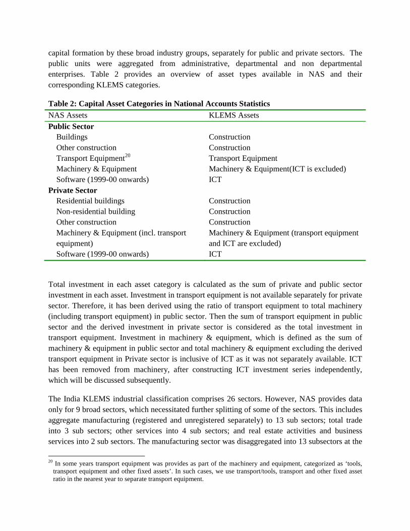
capital formation by these broad industry groups, separately for public and private sectors. The public units were aggregated from administrative, departmental and non departmental enterprises. Table 2 provides an overview of asset types available in NAS and their corresponding KLEMS categories.
Table 2: Capital Asset Categories in National Accounts Statistics NAS Assets KLEMS Assets
Public Sector Buildings Construction Other construction Construction Transport Equipment20 Transport Equipment Machinery & Equipment Machinery & Equipment(ICT is excluded) Software (1999-00 onwards) ICT Private Sector Residential buildings Construction Non-residential building Construction Other construction Construction Machinery & Equipment (incl. transport equipment)
Machinery & Equipment (transport equipment and ICT are excluded)
Software (1999-00 onwards) ICT
Total investment in each asset category is calculated as the sum of private and public sector investment in each asset. Investment in transport equipment is not available separately for private sector. Therefore, it has been derived using the ratio of transport equipment to total machinery (including transport equipment) in public sector. Then the sum of transport equipment in public sector and the derived investment in private sector is considered as the total investment in transport equipment. Investment in machinery & equipment, which is defined as the sum of machinery & equipment in public sector and total machinery & equipment excluding the derived transport equipment in Private sector is inclusive of ICT as it was not separately available. ICT has been removed from machinery, after constructing ICT investment series independently, which will be discussed subsequently.
The India KLEMS industrial classification comprises 26 sectors. However, NAS provides data only for 9 broad sectors, which necessitated further splitting of some of the sectors. This includes aggregate manufacturing (registered and unregistered separately) to 13 sub sectors; total trade into 3 sub sectors; other services into 4 sub sectors; and real estate activities and business services into 2 sub sectors. The manufacturing sector was disaggregated into 13 subsectors at the
20 In some years transport equipment was provides as part of the machinery and equipment, categorized as ‘tools,
transport equipment and other fixed assets’. In such cases, we use transport/tools, transport and other fixed asset ratio in the nearest year to separate transport equipment.

2 digit level of NIC 1998 using ASI and NSSO data, which will be discussed in detail subsequently. Investment series in service sector has been split into sub sectors using two alternative approaches – value added shares, and capital/labor ratio in the higher aggregate industry. However, the final data used are based on value added shares, as our sensitivity analysis did not show a significant difference between the two.
Table 3: Asset categories in ASI ASI Assets KLEMS Assets Land Excluded Buildings Buildings and Construction Plants & Machinery Machinery &Equipments ( ICT
is excluded) Transport Equipment Transport Equipment Computer Equipment including Software (from 1998) ICT equipments Pollution control equipment (from 2000) Machinery and Equipments
In order to split the aggregate capital formation in organized manufacturing sector into 13 KLEMS sectors, we use the Annual Survey of Industries. However, the published data does not provide any asset wise information; it consists of only the aggregate capital formation or the book value of fixed capital. The usual approach followed by most studies in the past is to measure gross investment as the difference between book value of asset in period t and in period t-1 and add depreciation in period t to that. This approach has the deficiency of comparing two year’s data, where the number of firms/factories might be different. In particular, while using this approach at industry level, for detailed asset categories, it might generate massive negative investment. We follow an alternative approach, following ASI’s definition of gross fixed capital formation (GFCF). ASI defines GFCF as actual additions (newly purchased, second hand and own construction) minus deductions plus depreciation adjustment for discarded assets during the year. This approach is based on a single year’s sample and helps to avoid potential huge negative investment series, and is also consistent with published ASI GFCF series. The yearly detailed volumes beginning 1964-65 were used to derive the gross fixed capital formation by asset type directly.21 For the years 1964-1978, the relevant data are obtained from published detailed volumes. For the period, 1983-84 to 2008-09 ASI has generated detailed tables from Block C of ASI schedule that contain data on fixed assets. Missing years are interpolated using the changes in investment using book value method. Table 3 provides an overview of the asset categories available in ASI, and the relevant asset categories in India KLEMS to which they are attributed. Though ASI provides investment in land, for reasons of NAS consistency we exclude it from the KLEMS database. Once investment in each of these assets and industries are generated using
21 The Annual Survey of Industry provided information on the following categories- land, buildings, plant &
machinery, transport equipment, computer equipment including software, pollution control equipment and others. These categories were aggregated into the same four asset classification as described in footnote 30.

ASI data, we apply this industry-asset distribution to the published NAS GFCF series for organized manufacturing sector. It may also be noted that from 1960-61 to 1971-72, ASI data are for the census sector and from 1973-74 on wards they are for the factory sector. In order to make these two series comparable over years, we convert the data prior to 1972 to factory sector using the factory/census ratio in 1973. Thus, after these adjustments, we obtain investment data for 13 manufacturing sectors, by asset types, consistent with the NAS aggregate.
Table 4: Asset categories in NSSO
45th round 51st round 56th round 62nd Round KLEMS asset Land Land excluded Building Construction Land &
Buildings Land & Buildings
Construction (land is excluded)
Other construction
Construction
Building & other construction
Construction
Plant & machinery Plant & machinery
Plant and machinery
Plant and machinery
Machinery & Equipment
Transport Equipments
Transport Equipments
Transport equipment
Transport equipment
Transport Equipment
Tools Machinery & Equip.
Other fixed assets
Machinery & Equip.
Tools and other fixed assets
Tools &other fixed assets
Tools and other fixed assets
Machinery & Equip.
Software & hardware
ICT equipment
Note: in all the cases, if ICT assets are not separately provided, they are excluded from machinery equipment, after estimating ICT investment independently (see section on ICT investment). For 56th and 62nd rounds, land is separated from land & buildings using land/land & building ratio from 51st round.
The data required for creating the gross investment series for the 13 unorganized segments of the
manufacturing sector are obtained from various rounds of NSSO surveys on unorganized
manufacturing. We use 4 rounds of NSSO surveys that cover the period 1989-2006. These are
45th round (1989-90), 51st round (1994-95) 56th round (1994-95) and 62nd round (2005-06). Unit
level data has been aggregated to 13 KLEMS sectors using the appropriate concordance tables.
NSSO provides net addition to owned assets during the reference year within the block of fixed
assets, and we use this as a measure of our investment. Asset classification in NSSO has changed
over various rounds, and therefore, we have tried to match these with our KLEMS classification
as shown in Table 4. The investment series arrived at for four rounds were interpolated to obtain
the annual time series of unorganized gross fixed capital formation by asset type. As in the case

of registered sector, once the investment by asset types across industries are constructed, the
asset-industry distribution is applied to the published NAS aggregate GFCF in unregistered
manufacturing to obtain NAS consistent GFCF by asset type and industries.
4.2 Investment in ICT assets
Since official statistics on ICT investment is still not comprehensive in India, we rely on
alternative sources to impute ICT investment. However, whenever the information is available
from official sources, we exploit such information, and ensure consistency with official statistics.
Since these estimates are still preliminary, we shall further improve the data if better information
is available. Following the standard practice, we define ICT investment as the investment in
computers or IT hardware, communication equipment and software. The available information
on ICT investment in India include software investment from NAS since 1999-00,22 ASI’s ICT
investment series in organized manufacturing sectors since 1998, NSSO 62nd round data on ICT
investment in unorganized manufacturing, CMIE’s PROWESS firm level data on gross fixed
assets in hardware, software and communication equipment (1989-2009) and World Information
Technology and Services Alliance (WITSA)23 ’s estimates on ICT spending by broad sectors of
the economy since 2000. We make use of all these information in our ICT investment estimates
along with investment data available by commodities in input-output tables. It may be noted that
there have been attempts in the past to estimate ICT investment in Indian economy. For instance
Jorgenson and Vu (2005) have estimated ICT investment for aggregate economy in a cross-
section of countries, including India. They apply United States’ ICT investment to ICT spending
ratio to WITSA ICT spending data for India, to obtain aggregate economy ICT investment.
However, this approach may produce a severe bias in the estimated investment. For instance, as
argued by de Vries et al, (2007) it might overestimate the actual ICT investment in developing
countries, as the investment/spending ration in developing countries might be lower than that of
the United States. On the other hand, it is also possible that most of the ICT spending in
developing countries is in the form of investment, as consumption spending on ICT in low
income countries would be relatively low compared to the US, and therefore, this approach
might underestimate the volume of ICT investment in developing countries. In any case, the use
of US investment to spending ratio to impute investment in India does not seem to be
appropriate. Apart from this, their estimates are not sufficient for our purpose, as their estimates
are available only for the total economy; we require investment by industries. In addition, we
prefer to be consistent with the available official data, which is not the case with Jorgenson and
22 Adopting the suggestions of 1993 System of National Accounts (SNA), NAS has included software in its capital formation data. However, it does not include own-account software. 23 WITSA provides ICT spending data in a cross section of countries through their Digital Planet Report. See http://www.witsa.org/

Vu. In what follows, we describe the approach we follow to construct ICT investment in Indian
economy.
Total economy ICT investments (for hardware and communication equipment) series is arrived
at using the commodity flow approach.24 In this approach, investment in hardware and
communication equipment can be estimated using the information on the total domestic
availability of these goods and its investment component. This requires the use of input-output
tables, in combination with NAS and trade statistics. We define the investment in ICT asset i as:
( )( )tititiIOsi
IOsi
IOsi
IOsi
ti XMYXMY
II ,,,
,,,
,, −+
−+= (5)
where Ii,t is the current investment, Y is gross domestic output, M is imports and X is exports.
Superscript IO refers to input-output tables, i.e. for instance, IOsiI , indicates investment in asset
type i (since we consider computer hardware and communication equipment, i=1,2, i.e. hardware
and communication equipment) in year s (where s is the benchmark year for IO table) obtained
from input-output table. All other variables without the superscript IO are time-series data
obtained from the NAS. Following the previous studies, we define industry 30 according to ISIC
3.1 (office equipment and machinery) as computer hardware and industry 32 (radio, TV and
communication equipment) as communication equipment. We obtain investment in hardware
and communication equipment, along with total domestic output, imports and exports for 6
benchmark years, 1983-84, 1989-90, 1993-94, 1998-99, 2003-04, 2006-07 from input-output
tables published by the Central Statistical Organization (CSO). There is no strict concordance
between ISIC 3.1 and India’s input-output table classification, and therefore, we consider the
Indian IO sector office computing and accounting machinery as hardware, communication
equipment and electronic equipment including TV as communication equipment. This
information is used to compute the first part of equation (5). Then, using time-series data on
gross output obtained from India KLEMS25 output database, and exports and imports obtained
from UN-comtrade statistics, we construct a series of ICT investment using equation (5).
This approach allows us to generate investment series only for total economy, as an industry
break-down is not possible with input-output table. Moreover, this method cannot be used to
infer any information on software investment, as the main source of data for this approach, i.e.
input output table, contains no information on software. de Vries et al (2007) suggest using the
elasticities of hardware to software investment, estimated using a fixed effect panel regression of
24 See Timmer and van Ark (2005) and de Vries et al (2007) for a good description of the commodity flow approach. 25 India KLEMS provides output and value added data, consistent with National Accounts Statistics. See the
Chapter on value added series.

software on hardware and a set of control variables. We follow this approach, but not using
econometric techniques. Apart from the input-output tables, there are other sources as well, from
where we can obtain information about the ICT investment in Indian industries. For instance,
latest National Accounts Statistics (NAS) provides investment in software for total economy,
Annual Survey of Industries (ASI) provides fixed capital in ICT during 1999-2008 for organized
manufacturing sector and NSSO surveys on unorganized manufacturing 62nd round provides ICT
investment data in unorganized manufacturing for the year 2005. In addition, Centre for
Monitoring Indian Economy (CMIE)’s firm-level database Prowess provides gross fixed assets
in hardware, software and communication equipments for companies categorized under NIC
1998. We use all these information to break down aggregate investment series generated using
commodity flow approach, to sectoral investment series.
In order to arrive at software investment series, we first compute software-to-hardware ratio for
years after 2000. We use the information on software series from NAS and the hardware data
obtained using the commodity flow approach. This ratio has been extrapolated linearly
backwards until 1970 to generate the software series for previous years. This provides us a
complete series of ICT investment, hardware, software and communication, for total economy
for the period 1970-2008.
For organized manufacturing sector, total ICT is computed as the sum of registered and non-
registered segments for the year 2008 by summing ASI and NSSO data on ICT investments.
Subsequently, we compute the ICT/machinery ratio for total manufacturing (organized plus
unorganized) for 2008, and this ratio has been extrapolated backward until 1999, using the
changes in ICT/machinery ratio for organized sector obtained from ASI data. For years 1989-99
the same has been computed using the changes in ICT/machinery ratio computed from Prowess
firm level data, aggregated to KLEMS 26 sectors. For 1970-89, the ratio has been extrapolated.
Using the time series of ICT/machinery ratio, along with the data on investment in machinery,
we compute a complete series of ICT investment series for total manufacturing segment for
1970-2008. This has been sub-dived into hardware, software and communication, assuming the
composition as in the aggregate sector. For non-manufacturing sectors, we first compute
ICT/machinery ratio from Prowess data, and apply to total machinery series to impute first set of
ICT investments. However, this series will not be consistent with the ICT series obtained using
commodity flow approach (we obtain the non-manufacturing segment from commodity flow
approach, after subtracting the manufacturing sector data from total economy). Therefore, we
apply the industry distribution obtained from Prowess-based derived ICT series to aggregate
non-manufacturing sector data obtained using commodity flow approach, in order to arrive at
industry wise estimates. The estimated ICT investment has been subtracted from the reported

machinery and equipment investment in all the sectors, to obtain the non-ICT machinery
investment.
As indicated before, this is a preliminary set of data which needs to be improved significantly.
There are many problems in the approach we followed, which includes, inconsistency between
aggregated firm level data and published aggregate data (e.g. ASI ICT/to aggregate investment
ratio is quite different from PROWESS aggregates for total manufacturing for years in which
both data are available), and the assumption of same annual changes in ICT/non-ICT ratio in
registered and unregistered manufacturing. In addition, there are alternative sources (e.g.
WITSA) to explore and the available information can be used in different ways, including
econometric approaches. These options will be explored in the future, and a sensitivity analysis
will be performed to understand the deviation of the final estimates from alternative approaches.
4.3 Asset wise Investment Prices
In order to compute asset wise capital stock using PIM (equation 3) and rental price (equation 4),
we require asset wise investment price deflators. CSO has provided asset wise deflators for all
the three asset type with base 1999-2000. These deflators are directly used for all the non-ICT
assets. Price measurement for ICT assets has been an important research topic in recent years, as
the quality of those capital goods has been rapidly increasing. Until recently, large differences
existed in the methodology to obtain deflators for ICT equipment between countries, and the use
of a single harmonised deflator across countries was widely advocated and used (Schreyer 2002;
Colecchia and Schreyer 2001; Timmer and van Ark 2005). This deflator was based on the US
deflators for computer hardware, which were commonly seen as the most advanced in terms of
accounting for quality changes using hedonic pricing techniques (Triplett 2006). For India, we
use the harmonisation procedure suggested by Schreyer (2002), where the US hedonic deflators
are adjusted for India’s domestic inflation rates.
4.4 Initial Stock, Depreciation Rates and Rate of Return
As is evident from equations 1 to 4, our estimates of capital input requires time-series data on
asset wise capital stock. Capital stock has been constructed using perpetual inventory method
(PIM), where the capital stock (S) is defined as a weighted sum of past investments with weights
given by the relative efficiencies of capital goods at different ages, which requires data on
current investment by asset types, investment prices by asset types and depreciation rate. Also,
for the practical implementation of PIM to estimate asset wise capital stock, we require an
estimate of initial benchmark stock (see Erumban, 2008b for an in-depth discussion on this
issue). NAS provides estimates of net capital stock since 1950 for all the broad sectors in its
Statement 17: Net Fixed Capital Stock by industry of use. We take the NAS estimate of real net

capital stock in 1950 (in 1999-2000 prices) as our benchmark stock for all non-manufacturing
sectors, and for manufacturing sectors the same is taken for the year 1964. 26 However, since the
NAS estimate is available only for broad sectors and for aggregate capital, we use our industry-
asset distribution of GFCF in order to create net fixed capital stock estimates by asset type for all
the 26 sectors. NAS also provides detailed tables on assumed life of assets used for computing
capital stock, for private units, administrative units as well as departmental and non departmental
units by asset types.27 We use these estimates of lifetime to derive appropriate depreciation rates
for non-ICT assets, using a double declining balance rate. We have used 80 years as assumed life
of buildings, 20 years for transport equipments, and 25 years for machinery and equipments. The
depreciation rates for ICT assets- hardware and software and communication equipments were
taken from the EU KLEMS. The final depreciation rates used in the study are given in Table 5
by asset type. Subsequently, we build our capital stock series by asset types for all the 26
industries using our GFCF series from 1950 (1964) onwards for the non-manufacturing
(manufacturing) sector.
Table 5: Depreciation rates used in the computation of capital input Asset types Depreciation rate (%)
Buildings and Constructions 2.5
Transport Equipment 10.00
Non-ICT Machinery 8.00
Hardware and Software 31.5
Communication Equipment 11.5
Note: depreciation rates are derived using NAS life times for each asset assuming a double declining balance rate. Source: NAS and EU KLEMS Our measure of capital input is arrived using equation (1), for which we also require estimates of
rental prices (see equation 4). Assuming that the flow of capital services is proportional to the
capital stock at individual asset level, aggregate capital flows can be obtained using a translog
quantity index by weighting growth in the stock of each asset by the average shares of each asset
in the value of capital compensation, as in (1). The rate of return (i) in equation (4) represents the
opportunity cost of capital, and can be measured either as internal (or ex post) rate of return, or as
an external (ex ante) rate of return.28 This issue will be addressed in the further revisions of the
data. The present version of the database uses an external rate of return, proxied by average of
return on government securities and prime lending rate obtained from the Reserve Bank of
26 This choice is driven by the fact that the first year of availability of ASI data is 1964-65. 27 Chapter 26, National Accounts Statistics -Sources and Methods, CSO (2007) 28 We do not intend to delve into the controversies over the use of internal vs. external rate of return in the context of
productivity measurement. Rather, given that this is the first version of our data, we use the external rate and in a later stage, we will also use internal rates. See Erumban (2008a and b) for a discussion on these issues.

India29. Therefore, we use a real rate, which is net of capital gain. Hence, the capital gain
component in equation (4) is excluded while estimating rental price using external rate of return,
obtaining
Itkkt
Itk
Ktk pipp ,
*1,, δ+= − (5)
where i* is the real rate of return, nominal interest rate adjusted for CPI inflation rate.
5. Estimates of capital Input for aggregate economy and its 26 sectors
Table 6 provides an overview of investment and capital structure in India, in terms of average
shares of different asset types in aggregate nominal capital formation and real capital stock. A
general picture that is seen in almost all sectors is that of an increasing share of construction
investment, and declining share in the capital stock. The decline in investment share of
construction is observed only in agriculture, while the mining and quarrying, construction and
service sector shows more prominent increase in the construction investment share. The decline
in agriculture is compensated predominantly by an increase in the machinery investment.
Though the share of ICT investment and capital stock has increased marginally in the 2000s
compared to the 1980s and 1990s, they still remain to be small in almost all sectors, with the
manufacturing sector showing the highest share.
Table 6: Asset structure of Investment and Capital stock in Indian economy, 1980-2013
1980-99 2000-13 1980-13 1980-99 2000-13 1980-13
Investment share in GFCF Share in real capital stock
Total Economy Construction 53.4 57.4 55.0 78.8 69.9 75.4 Machinery 37.7 34.3 36.4 17.9 25.0 20.6 Transport Eq 8.9 8.2 8.7 3.3 5.1 4.0 Agriculture Construction 85.3 73.1 80.7 95.6 87.7 92.5 Machinery 12.0 21.0 15.4 3.8 10.0 6.2 Transport Eq 2.7 5.8 3.9 0.6 2.3 1.3 Mining and Quarrying Construction 41.5 52.4 45.9 58.3 61.2 59.4 Machinery 56.7 43.1 51.2 40.4 36.2 38.8 Transport Eq 1.7 4.5 2.9 1.3 2.5 1.8 Manufacturing Construction 28.9 30.9 29.7 50.2 42.8 47.4 Machinery 60.1 56.4 58.6 44.3 48.4 45.8 Transport Eq 11.0 12.7 11.7 5.5 8.8 6.8 29 Handbook of Indian Statistics, Reserve Bank of India, Annual volumes.

1980-99 2000-13 1980-13 1980-99 2000-13 1980-13
Investment share in GFCF Share in real capital stock
Electricity, Gas and Water Supply Construction 47.9 50.4 48.8 71.0 65.5 68.9 Machinery 51.6 48.4 50.4 28.8 34.0 30.8 Transport Eq 0.5 1.2 0.8 0.2 0.5 0.3 Construction Construction 20.9 27.9 23.7 35.5 33.6 34.8 Machinery 65.4 58.4 62.5 56.4 55.1 55.8 Transport Eq 13.7 13.7 13.8 8.2 11.3 9.4 Services Construction 69.6 74.1 71.3 88.4 83.2 86.4 Machinery 18.8 19.2 19.0 7.6 12.4 9.5 Transport Eq 11.6 6.6 9.7 4.0 4.3 4.1
Source: India KLEMS database
Figure 1: ICT share in aggregate capital stock, Total economy and broad sectors
Source: India KLEMS database
In Figure 1, we provide a further industry break-up of ICT capital stock, which reveals that the manufacturing sector leads in ICT share. In particular, it is the machinery producing sector (KLEMS sector 29) that has witnessed the highest increase in ICT share over years. Even though the overall service sector shows only moderate increase in ICT share in total capital stock, a detailed look at the industries reveal that financial services have witnessed a faster increase in ICT share, particularly since the late 1990s. In the next section, we present estimates of capital
0.00
0.50
1.00
1.50
2.00
2.50
3.00
3.50
4.00
19
80
19
81
19
82
19
83
19
84
19
85
19
86
19
87
19
88
19
89
19
90
19
91
19
92
19
93
19
94
19
95
19
96
19
97
19
98
19
99
20
00
20
01
20
02
20
03
20
04
20
05
20
06
20
07
20
08
Agriculture
Mining and
Quarrying
Manufacturing
Electricity, Gas and
Water Supply
Construction
Services
Total economy

input for the aggregate economy and its broad sectors – agriculture, manufacturing, industry and services. Subsequently, we also provide estimates of capital services for the 26 KLEMS sectors.
5.1 Capital services in the disaggregate 26 KLEMS sectors
Aggregate capital service growth rates for each of the 26 KLEMS sector has been calculated
using asset wise investment series at disaggregate industry level, by employing equation (1). In
Table 7 we provide the sectoral growth rates of aggregate capital services, and the contribution
of equipment and non-equipment capital to aggregate capital service growth. Almost all sectors
of the economy have shown a high capital service growth rate in the both sub-periods (1980-99
and 2000-11). In particular, out of 26 sectors 15 sectors have shown a faster capital service
growth in the 2000s, compared to that of the 1980s and 1990s. This includes agriculture, hunting,
forestry & fishing, manufacturing nec, construction, trade, transport services, real estate,
education, health and other services. Sectors that witnessed a sharp decline in average capital
service growth rate include rubber & plastics, coke & refined petroleum, other non-metallic
mineral, pulp, paper , printing & publishing and textiles, leather & footwear, while most other
sectors have shown either an increase or have maintained a comparable growth rate in both
periods. In general the manufacturing sectors seem to have registered higher capital service
growth rate, perhaps due to rapid expansion of investment in the sector. Service sector also show
an increase in the capital services growth rate, suggesting an expansion of investment, though the
pace of expansion is not as large as in the manufacturing. Within the service sector, sectors
transport & storage, education and health have shown impressive capital service growth rates. It
may be noted that the latter three sectors also involve significant public sector investment. It is
often argued that in most developing countries, only less than half of the public investment
spending is translated into capital and therefore considering these investments would result in an
exaggeration of actual capital stock in these countries (see Pritchett, 2000). The argument here is
that the objective function of governments need not be profit maximization, while it is the base
of conventional treatment of capital in the literature.
The table also provides the contribution of equipment and non-equipment capital to aggregate
capital service growth rate. The contribution of equipment has witnessed the largest increase in
the 2000s in pulp, paper, printing & publishing. Other sectors that had an improvement in
equipment contribution include agriculture, hunting, forestry and fishing, post &
telecommunications, education, health & social work and financial intermediation. In case of
non-equipment contribution to capital services, hotels & restaurants, public administration,
mining & quarrying, machinery, nec. and textiles, leather & footwear have depicted the major
improvement in the 2000s.

Table 7: Contribution of equipment and non-equipment capital to aggregate capital service growth rates: 26 KLEMS sectors, 1980-2011 Capital service growth rates Contribution (%) of Equipment Contribution (%) of non-Equipment
Industry 1980-99 2000-11 1980-11 1980-99 2000-11 1980-11 1980-99 2000-11 1980-11
01 to 05 3.16 5.56 4.05 23.4 40.1 31.9 76.6 59.9 68.1
10 to 14 8.15 7.75 8.17 67.1 53.6 62.0 32.9 46.4 38.0
15 to 16 7.49 7.61 7.42 69.7 65.1 67.9 30.3 34.9 32.1
17 to 19 9.79 6.92 8.62 77.4 64.6 73.3 22.6 35.4 26.7
20 7.86 7.78 7.80 70.0 62.0 67.4 30.0 38.0 32.6
21 to 22 8.69 5.42 7.53 54.3 89.2 64.1 45.7 10.8 35.9
23 16.40 11.32 14.21 88.4 91.3 88.9 11.6 8.7 11.1
24 5.57 4.68 5.18 80.6 73.5 78.1 19.4 26.5 21.9
25 16.17 7.07 12.84 81.6 73.7 79.8 18.4 26.3 20.2
26 12.45 8.90 11.10 81.5 69.8 78.0 18.5 30.2 22.0
27 to 28 7.82 8.42 8.39 82.0 76.3 79.9 18.0 23.7 20.1
29 9.15 8.75 9.09 77.5 64.4 72.4 22.5 35.6 27.6
30 to 33 7.28 7.83 7.33 80.9 70.0 76.0 19.1 30.0 24.0
34 to 35 9.09 10.08 9.33 82.6 82.0 82.0 17.4 18.0 18.0
36 to 37 7.18 9.56 8.18 64.9 64.1 65.1 35.1 35.9 34.9
40 to 41 6.64 5.16 6.14 60.1 57.0 59.2 39.9 43.0 40.8
45 6.73 16.37 10.36 81.0 79.1 79.6 19.0 20.9 20.4
50 to 52 5.52 10.76 7.62 17.9 22.1 19.6 82.1 77.9 80.4
55 7.75 9.84 8.75 69.7 39.4 55.9 30.3 60.6 44.1
60 to 63 3.77 7.84 5.36 77.1 79.5 78.5 22.9 20.5 21.5
64 9.23 9.37 9.25 51.7 68.6 58.5 48.3 31.4 41.5
65 to 67 9.93 7.06 8.62 69.6 75.0 70.7 30.4 25.0 29.3
75 5.67 6.04 5.89 40.6 20.4 32.5 59.4 79.6 67.5
80 8.98 14.03 10.89 49.5 55.9 52.5 50.5 44.1 47.5
85 9.98 14.63 11.78 49.0 55.9 52.2 51.0 44.1 47.8
70 to 74, 90 to 96 3.50 8.26 5.27 8.95 10.92 10.48 91.05 89.08 89.52
Notes: Capital service growth rates are calculated using equation (1) for each industry. Contributions are the sum of individual assets 'Contributions are in percentages, and will add upto 100.

5.2 Capital services in the aggregate economy and its broad sectors
Aggregate capital service growth rates for the aggregate economy and its broad sectors are
calculated using two alternative approaches. The first is to use investment series aggregated
across industries, and then compute capital service growth rates using equation (1). The second is
to use the computed capital service growth rates for each industry (as presented in the previous
section) and then compute the aggregate capital service growth rates (for total economy and
broad sectors) using a Tornqvist quantity index, which is a discrete time approximation to a
Divisia index. In this aggregation approach we weight sectoral capital service growth rates using
annual moving weights based on averages of the sectoral share in total capital compensation, in
adjacent points in time. A major advantage of the Tornqvist index is that it belongs to the
preferred class of superlative indices (Diewert 1976). More precisely, it exactly replicates a
translog model which is highly flexible, that is, a model where the aggregate is a linear and
quadratic function of the components and time. The difference between these two aggregation
results may be attributed to the sectoral heterogeneity and therefore, the preferred measure is a
Tornqvist. Figure 2 provides the indices of aggregate capital services in total economy and its
broad sectors. Capital services show a faster growth rate in construction sector, compared to all
other sectors of the economy. This is in conformity with what we observed at the detailed
industry level. However, the service sector seems to show a faster growth in capital services in
the 2000s, compared to the 1980s and 1900s. Agricultural sector has witnessed only very
negligible growth in capital services over years; while capital services in construction sector
grew by almost 9 times over the period of a quarter of a century, capital services in the
agricultural sector has only increased by 3 times. These observations are further confirmed if we
look at the average growth rates of capital services in these sectors over the period, presented in
Table 8. Compared to the 1980s, both construction, service and agriculture sectors and
consequently the aggregate economy has witnessed a higher growth in the 2000s, with the
construction sector facing the highest among these three sectors. It may be noted that service
sector has been the fastest growing sector in Indian economy, which might be partly due to the
high growth of capital services in the sector. Manufacturing, on the other hand, is seen to have
shown a slight decline in its capital service growth rates. In Table 8 we also provide the average
growth rate of capital services using Tornqvist and simple aggregation procedures. The effect of
Tornqvist aggregation has been very minimal when the economy is taken as a whole, largely due
to negligible effect in agriculture and services. However, manufacturing sector shows a slightly
higher industry composition effect. The overall effect on aggregate growth is however, minimal.

Figure 2: Indices of Capital Services,
Note: Capital service growth rates are calculated using equation (1) and indexed to 1980. All the aggregates are obtained using a Tornqvist aggregation procedure. Source: India KLEMS database
Table 8: Growth rate of capital services, Aggregate Economy and broad sectors
Agriculture
Mining and Quarrying
Manufacturing
Electricity, Gas and Water Supply
Construction
Services
Total economy
Note: Capitals ervice growth rates are calculated using equation (1). Tornq. Are aggregate capital servie growth rates obtained by aggregating sectoral growth rates using a Tornqvist aggregation capitals ervidce ghrowth rates obtained using equation (1) with aggregate investment data for each broad sector. The difference btween the two (Tornq. - Simple), reflects the effect of sectoral heterogeneity.
In general, the overall picture is that of a high growth rate of capital input, both capital stock as well as capital services, in Indian economy and many of its subreasons for this, which might include the liberalization policies whichconstraints firms had to face in the past. Also, we may add a few caveats that can also have an effect on the measured capital input growth rates. Since we take official National Accounts data as our benchmark, part of the observed hreflection of the recent upward revisions in NAS, which has raised concerns over the reliability of the investment data (Shetty, 2006). Yet, another possibility is the low depreciation rates used
Figure 2: Indices of Capital Services, Aggregate Economy and broad sectors, 19802011(1980=100)
Note: Capital service growth rates are calculated using equation (1) and indexed to 1980. All the aggregates are obtained using a Tornqvist aggregation procedure.
Table 8: Growth rate of capital services, Aggregate Economy and broad sectors 1980-99 2000-11
3.2 5.6
8.1 7.7
9.6 8.0
6.6 5.2
6.7 16.4
7.1 9.8
8.2 8.7
ote: Capitals ervice growth rates are calculated using equation (1). Tornq. Are aggregate capital servie growth rates obtained by aggregating sectoral growth rates using a Tornqvist aggregation procedure. Sim,ple are aggregate capitals ervidce ghrowth rates obtained using equation (1) with aggregate investment data for each broad sector. The
Simple), reflects the effect of sectoral heterogeneity.
e overall picture is that of a high growth rate of capital input, both capital stock as well as capital services, in Indian economy and many of its sub-sectors. There are many possible reasons for this, which might include the liberalization policies which relaxed many capacity constraints firms had to face in the past. Also, we may add a few caveats that can also have an effect on the measured capital input growth rates. Since we take official National Accounts data as our benchmark, part of the observed higher growth rate of capital in the recent years may be a reflection of the recent upward revisions in NAS, which has raised concerns over the reliability of the investment data (Shetty, 2006). Yet, another possibility is the low depreciation rates used
nomy and broad sectors, 1980-
Note: Capital service growth rates are calculated using equation (1) and indexed to 1980. All the aggregates are
1980-11
4.1
8.2
8.1
6.1
10.4
6.2
6.6
ote: Capitals ervice growth rates are calculated using equation (1). Tornq. Are aggregate capital servie growth procedure. Sim,ple are aggregate
capitals ervidce ghrowth rates obtained using equation (1) with aggregate investment data for each broad sector. The
e overall picture is that of a high growth rate of capital input, both capital stock as sectors. There are many possible
relaxed many capacity constraints firms had to face in the past. Also, we may add a few caveats that can also have an effect on the measured capital input growth rates. Since we take official National Accounts data
igher growth rate of capital in the recent years may be a reflection of the recent upward revisions in NAS, which has raised concerns over the reliability of the investment data (Shetty, 2006). Yet, another possibility is the low depreciation rates used

in our capital measurement. Our knowledge of actual lifetime of capital assets in Indian economy is quite fragile, and therefore, we opted to use the NAS assumed lifetimes of assets to derive our depreciation rates. There exists diverging views on whether the lifetime of capital in developing countries will be different from the richer countries. For instance, they are viewed to be longer as the maintenance cost in developing countries will be lower (Summers and Heston, 1995). On the other hand, they could be shorter due to under-maintenance or low efficacy of public investment (Bu, 2004; Pritchett, 2000). These issues, however, warrant further detailed examination.
As noted before, when computing capital stock, most studies in the Indian context have either assumed no depreciation rates, or used a common depreciation rate for the aggregates of all assets, i.e. the total capital stock. These common depreciation rates hovers around 5 to 6 % (e.g. Bosworth and Collins, 2008; Goldar, 1986a). Since we use different depreciation rates for different asset types, we do not have an aggregate depreciation rate. However, we can derive the implicit aggregate depreciation rate, which is a weighted depreciation rate of individual assets, as δt=1-[ (St- It)/ St-1], with δ being the rate of depreciation, S and I are respectively capital stock and Investment in year t. The obtained rates are given in Appendix Table 1. The rates vary across industries and over period, due to changes in the asset composition. However, one general observation is that these rates appear to be low, particularly in the early years. The overall depreciation rate for the entire period is about 4%, with agriculture showing the lowest 3% and manufacturing showing the highest 6%. These rates are low compared to many previous aggregate studies in the context of India (Boseworth and Collins, 2008), and also many cross-country studies (e.g. Easterly and Levine, 2001). Also, compared to many cross-country databases such as the Penn World Tables (PWT) or EU KLEMS, the assumed depreciation rates for individual assets are low. For instance the PWT rates respectively for assets construction, machinery and transport equipment are 3.5%, 15% and 24% while the respective rates we used are 2.5%, 8% and 10%. The observed higher capital input growth rate may partly be due to low depreciation rates used in our analysis. This issue will be addressed in the further revisions of the data.
5.3 Capital services vs. Capital Stock: The composition effect
Table 9 provides the growth rates of capital stock by asset types for the aggregate economy and broad sectors. The growth rates of capital stock for 26 individual industries are provided in Appendix Tables 2 to 5. On average the aggregate capital stock in Indian economy has shown a lower growth rate than capital services (Table 7) during the same period. This higher growth of capital services is obviously due to faster growth of machinery and transport equipment, compared to construction capital (see the discussion that follows this section). Agriculture has shown less than 4 percentage growth in construction during the period, while the equipment capital in this sector has shown a remarkable growth rate (about 11 % o in transport equipment, and 9% in machinery and equipment). This might suggest that Indian agriculture has been increasingly becoming capital intensive; in particular the pace of mechanization in the sector has

been faster. Mining, manufacturing, electricity,construction and services show a similar pattern, where the equipment investment grows faster than construction investment, with the transport equipment dominating the machinery equipment for mining, manufacturing, electricity and costruction in both the periods. Interestingly, service sector has also shown a faster growth in machinery equipment than transport equipment. This is not surprising as the rapid expansion of service sector might have necessitated more intense use of non-residential construction such as office equipments.
Table 9: Growth Rate of Capital Stock by Asset types: Economy and Broad Sectors (% per annum) 1980-99 2000-11 1980-11 Economy Total Capital Stock 5.48 7.54 6.30 Construction 4.27 6.73 5.24 Transport Equipment 7.89 11.02 9.20 Machinery 8.29 8.79 8.50 Agriculture Total Capital Stock 2.91 5.03 3.71 Construction 2.68 4.11 3.22 Transport Equipment 8.03 15.75 10.71 Machinery 7.22 11.74 8.65 Mining and Quarrying Total Capital Stock 7.98 7.62 8.02 Construction 7.80 7.36 7.80 Transport Equipment 2.53 21.78 10.36 Machinery 8.50 7.22 8.17 Manufacturing Total Capital Stock 7.80 7.58 7.75 Construction 6.69 6.80 6.77 Transport Equipment 10.02 10.87 10.48 Machinery 8.66 7.58 8.26 Electricity, Gas and Water Supply Total Capital Stock 6.04 4.93 5.67 Construction 5.27 4.13 4.87 Transport Equipment 5.44 16.44 9.80 Machinery 8.07 6.17 7.43 Construction Total Capital Stock 6.91 16.19 10.42 Construction 7.48 15.50 10.62 Transport Equipment 7.16 19.36 11.89 Machinery 6.56 15.99 10.03 Service Total Capital Stock 4.48 8.08 5.87 Construction 4.04 7.60 5.41 Transport Equipment 6.45 9.25 7.63 Machinery 8.01 11.09 9.18 Source: India KLEMS database
We have argued that capital services that account for asset heterogeneity is a better and preferred
measure of capital input in productivity analysis than the standard measure of aggregate capital

stock. We compare the growth rates of capital stock measures,
capital services. The difference between the growth rates of capital service and capital stock is
often considered as an indicator of the quality of capital (Jorgenson, 2001). The premise of this
view is that the difference between growth of capital services and capital stock represents the
substitution toward assets with higher marginal products. For instance,
increases the quality of capital, as these equipments have relatively high marginal products. As is
evident from our methodology section, the difference between the two is primarily a result of
accounting for the changes in asset
different assets. Therefore, following Harper et al (1989), it is also called as a ‘composition
effect’. It is important to know the magnitude of the composition effect in order to understand
the possible bias in the measured contributions of capital and TFPG when capital stock measures
are used instead of capital services.
Figure 4: Capital composition effect, 1980
Note: capital composition effect is measures as capital service growth rate the aggregate capital services in each broad sector and total economy are obtained by aggregating sectoral capital service growth rates using Tornqvist aggregation.Source: India KLEMS database
Figure 4 provides the magnitude of capital composition effect averaged over the period 1980
2008. From the figure, it is evident that the composition effect is more prominent in the
electricity & gas, followed by manufacturing, agriculture
and in the 2000s. This suggest that the use of the conventional measure of capital stock would
30 It may be noted that our measure of capital stock is still different from most previous studies as we use asset wise depreciation rates while calculating capital stock of individual assets using PIM, and then aggregates across asset types. Most previous studies, apply PIM to aggregate common depreciation rate for all assets.
We compare the growth rates of capital stock measures,30 with that of our measures of
capital services. The difference between the growth rates of capital service and capital stock is
idered as an indicator of the quality of capital (Jorgenson, 2001). The premise of this
view is that the difference between growth of capital services and capital stock represents the
substitution toward assets with higher marginal products. For instance, a shift toward ICT capital
increases the quality of capital, as these equipments have relatively high marginal products. As is
evident from our methodology section, the difference between the two is primarily a result of
accounting for the changes in asset composition while aggregating capital services across
different assets. Therefore, following Harper et al (1989), it is also called as a ‘composition
effect’. It is important to know the magnitude of the composition effect in order to understand
ble bias in the measured contributions of capital and TFPG when capital stock measures
are used instead of capital services.
Capital composition effect, 1980-2011
Note: capital composition effect is measures as capital service growth rate minus capital stock growth rate, where the aggregate capital services in each broad sector and total economy are obtained by aggregating sectoral capital service growth rates using Tornqvist aggregation.
agnitude of capital composition effect averaged over the period 1980
. From the figure, it is evident that the composition effect is more prominent in the
manufacturing, agriculture and services both in the 1980s
s. This suggest that the use of the conventional measure of capital stock would
re of capital stock is still different from most previous studies as we use asset wise depreciation rates while calculating capital stock of individual assets using PIM, and then aggregates across asset types. Most previous studies, apply PIM to aggregate investment, often with no depreciation allowances or a common depreciation rate for all assets.
with that of our measures of
capital services. The difference between the growth rates of capital service and capital stock is
idered as an indicator of the quality of capital (Jorgenson, 2001). The premise of this
view is that the difference between growth of capital services and capital stock represents the
a shift toward ICT capital
increases the quality of capital, as these equipments have relatively high marginal products. As is
evident from our methodology section, the difference between the two is primarily a result of
composition while aggregating capital services across
different assets. Therefore, following Harper et al (1989), it is also called as a ‘composition
effect’. It is important to know the magnitude of the composition effect in order to understand
ble bias in the measured contributions of capital and TFPG when capital stock measures
minus capital stock growth rate, where
the aggregate capital services in each broad sector and total economy are obtained by aggregating sectoral capital
agnitude of capital composition effect averaged over the period 1980-
. From the figure, it is evident that the composition effect is more prominent in the
and services both in the 1980s &1990s
s. This suggest that the use of the conventional measure of capital stock would
re of capital stock is still different from most previous studies as we use asset wise depreciation rates while calculating capital stock of individual assets using PIM, and then aggregates across asset
investment, often with no depreciation allowances or a

overestimate TFPG in all the sectors of the economy, with manufacturing sector witnessing the
highest bias in the estimated TFPG. It is widely recognized that the
been growing very rapidly, particularly in the
the service sector is far below the one we observe in the
Figure 5: Capital composition effect:
Source: India KLEMS database
The capital composition effect observed at the aggregate economy and broad sectors are a
reflection of the sectoral composition effect, as is evident from Figure 5 where we provide the
composition effect in 26 KLEMS industrial sectors. As seen in the aggre
manufacturing industries have witnessed higher capital composition effect, which includes
paper, printing & publishing, transport equipment,
overestimate TFPG in all the sectors of the economy, with manufacturing sector witnessing the
highest bias in the estimated TFPG. It is widely recognized that the service sector in India has
been growing very rapidly, particularly in the 2000s, however, the capital composition effect in
the service sector is far below the one we observe in the agriculture sector.
Capital composition effect: 26 KLEMS industries, 1980-2011
The capital composition effect observed at the aggregate economy and broad sectors are a
reflection of the sectoral composition effect, as is evident from Figure 5 where we provide the
KLEMS industrial sectors. As seen in the aggre
manufacturing industries have witnessed higher capital composition effect, which includes
transport equipment, machinery, electrical and optical equipment,
overestimate TFPG in all the sectors of the economy, with manufacturing sector witnessing the
service sector in India has
, however, the capital composition effect in
The capital composition effect observed at the aggregate economy and broad sectors are a
reflection of the sectoral composition effect, as is evident from Figure 5 where we provide the
KLEMS industrial sectors. As seen in the aggregate picture,
manufacturing industries have witnessed higher capital composition effect, which includes
machinery, electrical and optical equipment,

basic metals and chemicals sectors. Within the service sector, transport & storage, health,
education, financial intermediation and communication sectors have witnessed relatively higher
capital quality improvement. Industries with lower composition effects are mostly manufacturing
sector industries, such as petroleum, Manufacturing nec and wood & products of wood.
Naturally, one would like to understand why the capital composition effect, or the quality of
capital, has grown so fast in India, in particular in the manufacturing sector. In order to explore
this, we provide the share of equipment capital in aggregate capital stock in total economy and
its broad sectors during 1980-2008 in Figure 6. The figure reveals that the share of equipment
capital (sum of machinery and transport equipment including ICT) in total capital stock in India
is increasing over years. Erumban (2008b) has shown a similar picture in a cross-section of
countries using Penn World Tables data. In particular, his results suggest increasing equipment
share in fast growing countries as part of their development process, confirming the importance
of equipment investment in attaining growth (De Long and Summers, 1991). The increasing
equipment share is particularly prominent in manufacturing and industry sectors, while the share
of equipment investment has not increased at a faster pace in the service sector. A detailed look
at the sectoral equipment share (see Appendix Figure 2) further reveals that the industrial sector
had higher equipment share throughout the period, with many manufacturing sectors facing a
faster increase in equipment share. This includes sectors electrical and optical equipment,
transport equipment, non-metallic minerals, basic metals, chemicals machinery. Within the
service sector financial intermediation and post and communication are the only sectors that
witnessed a remarkable increase in equipment share. Though construction sector shows a higher
equipment share in both sub-periods, it has witnessed only a marginal increase over years. As we
indicated before, investment in non-residential buildings might still be expanding in the service
sector, resulting in a relatively lower increase in the equipment share.

Figure 6: Equipment Share in Aggregate Capital Stock, 1980
Note: Equipment capital stock is defined
Source: Authors’ calculations
The increasing share of equipment capital will naturally lead to a faster growth of equipment
capital compared to non-equipment capital assets, which will have c
aggregate capital input growth. In Figure
with that of non-equipment capital stock in Indian economy. Evidently, the equipment capital
grows faster than non-equipment capital.
equipment growth is less prominent in
Equipment capital in manufacturing sector overtakes the growth of non
shows a faster growth since the early 1990s. Similarly, agriculture also shows a sharp increase in
equipment capital since the late 1990s.
increasing equipment share, by adding assets of higher marginal productivity
to deliver more capital services in short period of time, will result in higher capital service
growth rates compared to growth rates based on capital stock measures. This would suggest that
the use of capital stock growth rates would l
contribution of capital input to output growth and thereby overstate the TFPG.
Equipment Share in Aggregate Capital Stock, 1980-2011
Note: Equipment capital stock is defined as the sum of machinery and transport equipment (including ICT).
The increasing share of equipment capital will naturally lead to a faster growth of equipment
equipment capital assets, which will have consequences for the
aggregate capital input growth. In Figure 7 we also compare the growth of equipment capital
equipment capital stock in Indian economy. Evidently, the equipment capital
equipment capital. Also, the gap between equipment growth and non
equipment growth is less prominent in manufacturing compared to service sector
Equipment capital in manufacturing sector overtakes the growth of non-equipment capital and
th since the early 1990s. Similarly, agriculture also shows a sharp increase in
e the late 1990s. This faster growth of equipment capital, and the resultant
increasing equipment share, by adding assets of higher marginal productivity which are expected
to deliver more capital services in short period of time, will result in higher capital service
growth rates compared to growth rates based on capital stock measures. This would suggest that
he use of capital stock growth rates would lead to severe underestimation of the actual
contribution of capital input to output growth and thereby overstate the TFPG.
as the sum of machinery and transport equipment (including ICT).
The increasing share of equipment capital will naturally lead to a faster growth of equipment
onsequences for the
we also compare the growth of equipment capital
equipment capital stock in Indian economy. Evidently, the equipment capital
Also, the gap between equipment growth and non-
service sector and agriculture.
equipment capital and
th since the early 1990s. Similarly, agriculture also shows a sharp increase in
This faster growth of equipment capital, and the resultant
which are expected
to deliver more capital services in short period of time, will result in higher capital service
growth rates compared to growth rates based on capital stock measures. This would suggest that
ead to severe underestimation of the actual

Figure 7: Growth of Equipment capital stock vs. non: Growth of Equipment capital stock vs. non-Equipment capital stock, 1980=1Equipment capital stock, 1980=1

Note: EQ=Equipment capital stock; nEQ=non
sum of machinery and transport equipment (including ICT). Capital stock is indexed to the first year.
Thus the picture emerges is that of an
growth of the same in Indian economy, and its sub sectors, predominantly in the manufacturing
sector. The relationship between capital quality or composition effect and the observed
increasing share of equipment capital in India is more evident from Figure
scatter plots of change in equipment share against capital composition effect
economy. We observe a strong positive correlation between capital composition effect an
increasing equipment share. Moreover, equipment share and consequently capital composition
effect have shown an increasing trend in most of the years (as observed in our earlier graphs
also). Similar relationship is observed at the detailed industry leve
composition effect averaged across years, against average change in equipment share over the
period, across 26 KLEMS industries. We see a positive relationship in general, and a more
prominent one in the 2000s, suggesting more
consequently faster capital service growth rate. These observations further suggests that the use
of conventional measures of capital stock would overestimate the contribution of TFPG in Indian
economy, as the share of fast depreciating assets tend to show an increasing trend.
Figure 8: Change in Equipment Share and Capital Composition EffectEconomy 1980 to 2011
Note: Capital composition effect is measured as capital service growth rate minus cappositive relationship shows that higher the increase in the equipment share, higher the capital composition effectSource: Authors’ calculations
Note: EQ=Equipment capital stock; nEQ=non-equipment capital stock. Equipment capital stock is defined as the
sum of machinery and transport equipment (including ICT). Capital stock is indexed to the first year.
Thus the picture emerges is that of an increasing share of equipment capital, and also
growth of the same in Indian economy, and its sub sectors, predominantly in the manufacturing
The relationship between capital quality or composition effect and the observed
of equipment capital in India is more evident from Figure 8,
scatter plots of change in equipment share against capital composition effect
e observe a strong positive correlation between capital composition effect an
sing equipment share. Moreover, equipment share and consequently capital composition
effect have shown an increasing trend in most of the years (as observed in our earlier graphs
also). Similar relationship is observed at the detailed industry level also. In Figure
composition effect averaged across years, against average change in equipment share over the
KLEMS industries. We see a positive relationship in general, and a more
, suggesting more industries with increasing equipment share and
consequently faster capital service growth rate. These observations further suggests that the use
of conventional measures of capital stock would overestimate the contribution of TFPG in Indian
share of fast depreciating assets tend to show an increasing trend.
Change in Equipment Share and Capital Composition Effect, Aggregate
Note: Capital composition effect is measured as capital service growth rate minus capital stock growth rate. A positive relationship shows that higher the increase in the equipment share, higher the capital composition effect
equipment capital stock. Equipment capital stock is defined as the
sum of machinery and transport equipment (including ICT). Capital stock is indexed to the first year.
sing share of equipment capital, and also a faster
growth of the same in Indian economy, and its sub sectors, predominantly in the manufacturing
The relationship between capital quality or composition effect and the observed
8, which provides
scatter plots of change in equipment share against capital composition effect in the overall
e observe a strong positive correlation between capital composition effect and
sing equipment share. Moreover, equipment share and consequently capital composition
effect have shown an increasing trend in most of the years (as observed in our earlier graphs
l also. In Figure 9 we plot
composition effect averaged across years, against average change in equipment share over the
KLEMS industries. We see a positive relationship in general, and a more
s with increasing equipment share and
consequently faster capital service growth rate. These observations further suggests that the use
of conventional measures of capital stock would overestimate the contribution of TFPG in Indian
share of fast depreciating assets tend to show an increasing trend.
, Aggregate
ital stock growth rate. A positive relationship shows that higher the increase in the equipment share, higher the capital composition effect.
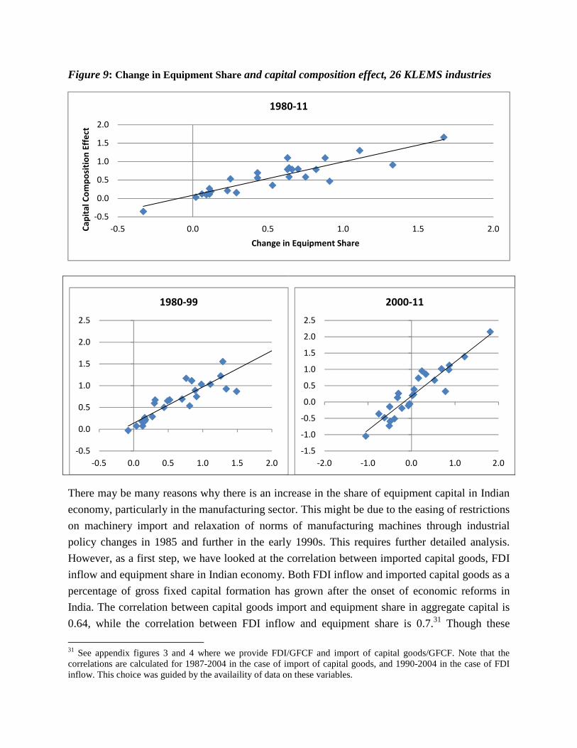
-0.5
0.0
0.5
1.0
1.5
2.0
-0.5 0.0 0.5 1.0 1.5 2.0Ca
pit
al
Co
mp
osi
tio
n E
ffe
ct
Change in Equipment Share
1980-11
Figure 9: Change in Equipment Share and capital composition effect, 26 KLEMS industries
There may be many reasons why there is an increase in the share of equipment capital in Indian
economy, particularly in the manufacturing sector. This might be due to the easing of restrictions
on machinery import and relaxation of norms of manufacturing machines through industrial
policy changes in 1985 and further in the early 1990s. This requires further detailed analysis.
However, as a first step, we have looked at the correlation between imported capital goods, FDI
inflow and equipment share in Indian economy. Both FDI inflow and imported capital goods as a
percentage of gross fixed capital formation has grown after the onset of economic reforms in
India. The correlation between capital goods import and equipment share in aggregate capital is
0.64, while the correlation between FDI inflow and equipment share is 0.7.31 Though these
31 See appendix figures 3 and 4 where we provide FDI/GFCF and import of capital goods/GFCF. Note that the correlations are calculated for 1987-2004 in the case of import of capital goods, and 1990-2004 in the case of FDI inflow. This choice was guided by the availaility of data on these variables.
-0.5
0.0
0.5
1.0
1.5
2.0
2.5
-0.5 0.0 0.5 1.0 1.5 2.0
1980-99
-1.5
-1.0
-0.5
0.0
0.5
1.0
1.5
2.0
2.5
-2.0 -1.0 0.0 1.0 2.0
2000-11

results may be taken as suggestive only, they are indicative of the possible reasons for the
increasing share of machinery capital in Indian economy. Thus evidently, our new measures of
capital shows a faster growth of capital services, as the share of equipment capital is increasing
and thereby adding more productive assets to the aggregate capital stock.
6. Conclusions
This paper provides new estimates of capital input for productivity analysis in Indian economy
and 26 sectors for the period 1980-2011. Compared to conventional measures of capital stock,
our measure of capital services are theoretically pertinent, as it takes asset heterogeneity into
account, while aggregating capital services. This is of particular importance, given the
importance of equipment investment for economic growth, which is growing faster in the Indian
economy. Measures of capital services are increasingly preferred in the international academic
sphere, over the conventional measures of capital stock. However there is hardly any attempt to
construct a proper measure of capital service in the Indian economy. This paper makes an
important contribution by providing estimates of capital services. Using several sources of
official data (including those which are not publically available), we construct aggregate capital
service measures, considering asset heterogeneity. We distinguish between asset types, non-ICT
machinery (construction, non-ICT machinery, transport equipment) and ICT machinery
(hardware, software and communication equipment). This distinction also helps us examine the
dynamics of investment composition in the Indian economy, in particular in terms of a change in
the composition favouring equipment investment.
Our results suggest an increasing share of equipment capital in the aggregate economy and its
broad sectors, dominantly in the manufacturing sector. While the service sector shows relative
lower growth in the transport equipment capital, manufacturing, industry and agriculture shows
high growth rates. This is particularly true in the 2000s, compared to the 1980s &1990s. A
detailed look at the disaggregated industry results further reveals faster growth of equipment
capital in many manufacturing sectors, which includes electronics, machinery and chemical
sectors, while a similar trend is observed only in a few service sectors, such as communication
and financial services. Our estimates of ICT investment suggest that the ICT intensity is still low
in most of the sectors. Though the ICT share has increased in manufacturing and services sectors
over years, the shares are still low.
The observed increase in equipment share has translated to a higher growth rate of our new
measure of capital input, compared to conventional measure of capital stock. The difference
between the two measures, the composition effect of capital, has seen to be quite high,
particularly in the electricity & gas and manufacturing sector. This measured gap between

conventional measure of capital stock and our improved measures of capital service will have
consequences for growth analysis. Therefore, it may be interesting to look into the causes of
increasing quality of capital in Indian economy, led primarily by an increasing share of
equipment capital. One may attribute the increasing share of machinery and equipment in
aggregate capital stock to the many policy reforms in the 1980s and 1990s that helped firms ease
many capacity constraints, and relaxed many restrictions on import of capital goods and foreign
direct investment, particularly in the manufacturing sector. These might have helped expand the
machinery investment in the economy, predominantly in the manufacturing sector. However, the
benefit of this has triggered to the other sectors of the economy as well, though not to the extent
of manufacturing. The effect of taking account of this quality aspect of measured capital input
would be that we will be able to measure the TFPG more precisely, by attributing that part of the
output growth that is due to the capital composition changes. In other words, we may see a
higher capital contribution to output growth, and a lower TFPG growth, which is close to reality,
than what have observed in the past by many studies. This will be further explored in the
productivity Chapter.
Notwithstanding the improvements we have made in the measurement of capital input for Indian
economy, it should be noted that our capital measures may still reflect any limitation of the
official data. Also there is still room for improvement, such as the use of alternate depreciation
pattern, which might have an effect on the measured growth rate of capital input and the
treatment of land. We assumed that the capital stock consists of (only) machinery, transport
equipment and construction, while the role of land as a capital input is not taken into account.
Even though some studies have shown that the contribution of land to aggregate growth is
negligible (e.g. Bosworth and Collins, 2008), it may still be an important aspect, particularly in
the agricultural sector. Similarly, we do not make a distinction between public and private
investment, which is often argued to be an important aspect in the context of developing
countries. However, a quick look at the investment structure of India reveals that the share of
public sector investment has been declining in the recent years. Yet another aspect is associated
with the measurement of rates of return and rental prices that are crucial for the proper
measurement of capital service growth rates. We assumed an external rate of return in our rental
price calculation. Nevertheless, an important issue in the context of rates of return is what should
be the ideal measure of the rate of return. There are different ways of deriving rate of return and
consequently rental prices, depending upon the assumptions one makes about their components.
Erumban (2008b) shows that the choice between an internal rate and an external rate has
empirical implications for aggregate capital services and thereby measured TFP growth rates,
while the growth rates are less sensitive to other alternatives. These issues warrant further
detailed examination and some of them will be addressed in the further revisions of the database.

Appendices
Appendix Table 1: Derived depreciation rate for aggregate capital
1965-75 1976-
Total Economy 3.4 3.8
Agriculture 2.6 2.8
Manufacturing 5.1 5.4
Industry 5.6 5.8
Services 3.3 3.4
Note: Aggregate depreciation rates (δ) are derived as stock and Investment in year t.
Appendix Figure 2: Equipment share in Aggregate capital stock,
Derived depreciation rate for aggregate capital
-86 1987-97 1998-11 1965-11
3.8 3.8 4.2 3.7
2.8 2.7 3.1 2.8
5.4 5.4 5.8 5.3
5.8 5.0 5.4 5.3
3.4 3.3 3.5 3.3
δ) are derived as δt=1-[(St- It)/ St-1], where S and I are respectively capital
: Equipment share in Aggregate capital stock, 26 industries, 1980
], where S and I are respectively capital
industries, 1980-2011

Appendix Figure 3: FDI inflow to Indian Economy, 1990-2008
Note: FDI/GDP is the ratio of foreign direct investment (FDI), direct and portfolio investment to current GDP; FDI/GFCF is the ratio of FDI to gross fixed capital formation Source: Reserve Bank of India
Appendix Figure 4: Import of Capital Goods, 1987-2008
Source: Reserve Bank of India Note: IMP_K/GDP is the ratio of imported capital goods to current GDP; IMP_K/GFCF is the ratio of imported capital goods to current gross fixed capital formation
0.0%
2.0%
4.0%
6.0%
8.0%
10.0%
12.0%
14.0%
16.0%
FDI/GDP
FDI/GFCF
0.0%
2.0%
4.0%
6.0%
8.0%
10.0%
12.0%
14.0%
16.0%
18.0%
19
87
-88
19
88
-89
19
89
-90
19
90
-91
19
91
-92
19
92
-93
19
93
-94
19
94
-95
19
95
-96
19
96
-97
19
97
-98
19
98
-99
19
99
-00
20
00
-01
20
01
-02
20
02
-03
20
03
-04
20
04
-05
20
05
-06
20
06
-07
20
07
-08
IMP_K/GDP
IMP_K/GFCF

Appendix Table 2: Growth rate of capital stock for two sub-periods and the whole period by 26 industries. Industry
No. Industry description 1980 2000 1980
to to to 1999 2011 2011
1 Agriculture, Hunting, Forestry and Fishing 2.91 5.03 3.71
2 Mining and Quarrying 7.98 7.62 8.02
3 Food Products, Beverages and Tobacco 7.01 7.38 7.04
4 Textiles & Leather Products 9.54 7.06 8.52
5 Wood and Products of wood 7.41 7.63 7.44
6 Pulp, Paper, Paper products, printing and publishing 7.99 4.38 6.70
7 Coke, Refined Petroleum products and Nuclear fuel 16.45 11.15 14.21
8 Chemicals and Chemical Products 5.25 4.64 4.97
9 Rubber and Plastic Products 15.52 7.06 12.44
10 Other Non-Metallic Mineral Products 11.70 8.95 10.64
11 Basic Metals and Fabricated Metal Products 7.38 8.31 8.05
12 Machinery, nec. 8.69 8.70 8.80
13 Electrical and Optical Equipments 6.34 7.76 6.75
14 Transport Equipment 8.12 9.65 8.60
15 Manufacturing, nec 7.49 9.09 8.16
16 Electricity, Gas and Water Supply 6.04 4.93 5.67
17 Construction 6.91 16.19 10.42
18 Trade 5.95 10.69 7.88
19 Hotels and Restaurants 7.21 10.35 8.63
20 Transport and Storage 3.03 6.96 4.57
21 Post and Telecommunication 8.81 8.49 8.65
22 Financial Services 9.02 6.42 7.92
23 Public Administration and Defence 4.93 6.09 5.45
24 Education 8.04 13.24 10.03
25 Health and Social Work 9.05 13.85 10.92
26 Other services 3.38 8.08 5.12
Source: India KLEMS database

Appendix Table 3: Growth rate of Construction for two sub-periods and the whole period by 26 industries.
Industry No.
Industry description 1980 2000 1980 to to to
1999 2011 2011
1 Agriculture, Hunting, Forestry and Fishing 2.68 4.11 3.22
2 Mining and Quarrying 7.80 7.36 7.80
3 Food Products, Beverages and Tobacco 6.37 6.63 6.37
4 Textiles & Leather Products 9.17 7.67 8.55
5 Wood and Products of wood 6.97 7.20 6.93
6 Pulp, Paper, Paper products, printing and publishing 7.10 1.42 4.98
7 Coke, Refined Petroleum products and Nuclear fuel 15.33 9.68 13.37
8 Chemicals and Chemical Products 4.53 4.32 4.42
9 Rubber and Plastic Products 14.29 7.04 11.70
10 Other Non-Metallic Mineral Products 10.03 9.19 9.65
11 Basic Metals and Fabricated Metal Products 5.97 7.90 6.94
12 Machinery, nec. 8.03 9.06 8.57
13 Electrical and Optical Equipments 4.59 7.58 5.73
14 Transport Equipment 5.91 8.07 6.78
15 Manufacturing, nec 7.99 7.92 7.96
16 Electricity, Gas and Water Supply 5.27 4.13 4.87
17 Construction 7.48 15.50 10.62
18 Trade 6.16 10.64 8.03
19 Hotels and Restaurants 6.46 11.70 8.71
20 Transport and Storage 2.00 4.27 2.89
21 Post and Telecommunication 8.23 5.95 7.31
22 Financial Services 7.67 4.97 6.62
23 Public Administration and Defence 4.55 6.15 5.23
24 Education 7.11 11.62 8.86
25 Health and Social Work 8.13 12.26 9.77
26 Other services 3.30 7.82 4.97
Source: India KLEMS database

Appendix Table 4: Growth rate of Machinery for two sub-periods and the whole period by 26 industries. Industry
No. Industry description-phase II 1980 2000 1980
to to to 1999 2011 2011
1 Agriculture, Hunting, Forestry and Fishing 7.22 11.74 8.65
2 Mining and Quarrying 8.50 7.22 8.17
3 Food Products, Beverages and Tobacco 7.49 7.97 7.52
4 Textiles & Leather Products 9.41 6.06 8.02
5 Wood and Products of wood 7.34 6.64 7.08
6 Pulp, Paper, Paper products, printing and publishing 10.18 7.94 9.45
7 Coke, Refined Petroleum products and Nuclear fuel 16.90 11.13 14.39
8 Chemicals and Chemical Products 5.55 4.68 5.13
9 Rubber and Plastic Products 15.93 6.83 12.59
10 Other Non-Metallic Mineral Products 13.42 7.86 11.29
11 Basic Metals and Fabricated Metal Products 8.63 7.82 8.68
12 Machinery, nec. 8.88 7.11 8.27
13 Electrical and Optical Equipments 7.97 7.78 7.62
14 Transport Equipment 9.92 10.12 9.78
15 Manufacturing, nec 7.42 8.95 8.06
16 Electricity, Gas and Water Supply 8.07 6.17 7.43
17 Construction 6.56 15.99 10.03
18 Trade 4.77 10.41 6.81
19 Hotels and Restaurants 8.50 7.47 8.23
20 Transport and Storage 8.45 11.22 9.36
21 Post and Telecommunication 10.45 11.13 10.66
22 Financial Services 10.86 7.46 9.63
23 Public Administration and Defence 5.94 7.75 6.75
24 Education 12.27 16.14 13.62
25 Health and Social Work 13.05 16.63 14.34
26 Other services 8.88 14.12 11.06
Source: India KLEMS database

Appendix Table 5: Growth rate of Transport Equipment for two sub-periods and the whole period by 26 industries. Industry
No. Industry description 1980 2000 1980
to to to 1999 2011 2011
1 Agriculture, Hunting, Forestry and Fishing 8.03 15.75 10.71
2 Mining and Quarrying 2.53 21.78 10.36
3 Food Products, Beverages and Tobacco 10.32 9.30 9.90
4 Textiles & Leather Products 14.11 9.14 12.21
5 Wood and Products of wood 11.75 11.91 11.90
6 Pulp, Paper, Paper products, printing and publishing
12.36 10.10 11.46
7 Coke, Refined Petroleum products and Nuclear fuel
11.02 21.62 14.86
8 Chemicals and Chemical Products 8.55 6.03 7.76
9 Rubber and Plastic Products 20.17 8.14 15.75
10 Other Non-Metallic Mineral Products 12.08 13.85 12.94
11 Basic Metals and Fabricated Metal Products 6.79 13.72 9.88
12 Machinery, nec. 12.42 12.64 12.52
13 Electrical and Optical Equipments 11.53 8.48 10.36
14 Transport Equipment 12.44 13.05 12.64
15 Manufacturing, nec 5.72 13.00 8.83
16 Electricity, Gas and Water Supply 5.44 16.44 9.80
17 Construction 7.16 19.36 11.89
18 Trade 4.54 13.91 8.13
19 Hotels and Restaurants 8.49 10.27 9.45
20 Transport and Storage 2.97 8.77 5.44
21 Post and Telecommunication 9.01 35.81 17.94
22 Financial Services 14.17 12.55 10.88
23 Public Administration and Defence 16.64 2.53 11.30
24 Education 13.03 20.17 15.87
25 Health and Social Work 13.87 20.68 16.63
26 Other services 9.86 17.86 13.33
Source: India KLEMS database

References
Ahluwalia, I.J. (1985), Industrial Growth in India. Stagnation since the Mid-Sixties, Oxford University Press, Delhi.
Ahluwalia, I.J. (1991), Productivity and Growth in Indian Manufacturing, Oxford University Press, Delhi.
Azeez E. A (2005), Domestic capacity utilisation and import of capital goods: Substitutes or complementary? Evidence from Indian capital goods sector , in Tendulkar, Mitra, Narayanan and Das (eds), India: Industrialisation in a Reforming Economy- Essays for K.L Krishna , New Delhi, Academic Foundation.
Balakrishnan, P. and K. Pushpangadan (1994), ‘Total Factor Productivity Growth in Manufacturing Industry: A Fresh Look’, Economic and Political Weekly, July 30, 2028-2035.
Banerjee Asit (1975), Capital Intensity and Productivity in Indian Industries, Macmillan, New Delhi
Basu S., J. Fernald, N. Oulton and S. Srinivasan (2003), "The Case of the Missing Productivity Growth: Or, Does Information Technology Explain Why Productivity Accelerated in the United States but not the United Kingdom?" NBER Macroeconomics Annual.
Bosworth, Barry and Susan M. Collins (2008), “Accounting for Growth: Comparing China and India,” Journal of Economic Perspectives, American Economic Association, Winter, 22(1): 45-66.
Christensen, L.R. and Jorgenson D.W. (1969), ‘The Measurement of US Real Capital Input,1929-1967,’ Review of Income and Wealth, 15, 293-320.
Colecchia A. and Schreyer P. (2001), ‘ICT Investment and Economic Growth in the 1990s: IS United States a Unique Case’, OECD STI Working Papers, pp 1-31,
Das, D.K. (2004), Manufacturing Productivity under Varying Trade regimes, 1980-2000, Economic and Political Weekly, January 31.
De Long B.J. and Summers L. (1991), ‘Equipment Investment and Economic Growth’, The Quarterly Journal of Economics, Vol. 106, No. 2. (May, 1991), pp. 445-502.
Denison, E.F.(1957), ‘Theoretical Aspects of Quality Change, Capital Consumption and Net Capital Formation’ in Problems of Capital Formation, NBER.
de Vries G, Mulder N, Dal Borgo M and Hofman A (2007), ‘ICT investment in Latin America: does IT matter for economic growth?’, Presentation to Seminario Crecimiento, Productividad y Tecnologías de la Información 29– 30 March 2007.

Diewert, W.E (1976), Exact and superlative index numbers, Journal of Econometrics, 4, 115-145.
Dholakia, B (1974), Sources of economic growth in India, Good Companion, Baroda, India
Erumban, A, A (2008a), Rental prices, rates of return, capital aggregation and productivity: Evidence from EU and US, CESifo Economic Studies, 3 (54), 499-533.
Easterly, W., Levine, R. (2001). “It’s not factor accumulation: Stylized facts and growth”. World Bank Economic Review 15, 177–219.
Erumban, A, A (2008b), Measurement and Analysis of Capital, Productivity and Economic Growth, SOM theses series, University of Groningen (available http://irs.ub.rug.nl/ppn/315102683).
Hashim, B.R. and M.M. Dadi (1973), Capital-Output Relations in Indian Manufacturing (1946-64), MS University, Baroda
Goldar B.N. (1981), “Some Aspects of Technological Progress in Indian Manufacturing Industries”, Ph.D. thesis, Delhi School of Economics, University of Delhi,
Goldar, B.N. (1986a), Productivity Growth in Indian Industry, Allied Publishers, New Delhi.
Goldar, B.N. (1986b), ‘Import Substitution, Industrial Concentration and Productivity Growth in Indian Manufacturing,’ Oxford Bulletin of Economics and Statistics, Vol. 48, No.2, 143-64.
Goldar, B.N and Renganathan, V.S (2008), Import penetration and capacity utilization in Indian industries, Working Paper no. E/293/2008, Institute of Economic Growth, Delhi.
Harper, M.J., E.R Berndt and D.O, Wood (1989), Rates of return and capital aggregation using alternative rental prices, in Jorgenson, D.W and R. Landau (eds.), Technology and Capital Formation, MIT Press.
Hulten, C.R. (1990), ‘The Measurement of Capital’, in: E.R. Berndt and J.E. Triplett (eds) Fifty Years of Economic Measurement, Studies in Income and Wealth, (Chicago: Chicago University Press for the National Bureau of Economic Research), pp. 119-152.
Jorgenson, D.W (1963), Capital theory and investment behavior, American Economic Review, 53 (2), 247-259.
Jorgenson, D.W and Z. Griliches (1967), The explanation of productivity change, Review of Economic Studies, 34, 249-283.
Jorgenson, D.W. (1989), “Capital as a Factor of Production,” in Jorgenson D.W.and Ralph Landau (1989), Technology and Capital Formation, Cambridge MA, MIT Press.

Jorgenson D.W. (2001), ‘Information Technology and The U.S. Economy’, American Economic Review, 91(1), 1-32.
Jorgenson, D.W. (2009), ‘A New Architecture for the U.S. national Accounts’, Review of Income and Wealth, Volume 55, Issue 1, pages 1–42, March 2009
Jorgenson D.W. and Stiroh K.J. (2000), ‘Raising the Speed Limit: U.S. Economic Growth in the Information Age’, Brookings Papers on Economic Activity, (1), 125-211
Jorgenson, D. W., Ho, M. S. and Stiroh, K. J. (2005), ‘Information Technology and the American Growth Resurgence’, MIT Press, Cambridge,
J Mohan Rao (1996), ‘Manufacturing Productivity Growth - Method and Measurement’, Economic and Political Weekly, November 2.
Krishna Raj and Mehta, S.S. (1968). "Productivity Trends in Large Scale Industries," Economic and Political Weekly, vol. 3, No 43, pp 1655-60.
Manna, G.C (2010), Current status of industrial statistics in India: Strengths and weakness, Economic and Political Weekly, XLV (46), 67-76.
Narasimham G. and J. Fabrycy (1974), “Relative efficiencies of organized industries in India, 1949-58”, Journal of Development Studies, Volume 10, Issue 2 January 1974
Nehru V. and Dhareshwar A. (1993), ‘New Estimates of total factor productivity growth for developing and industrial countries’, Policy Research Working Paper Series, No 1313, World Bank
OECD (2009), ‘Measuring Capital – OECD manual: Measurement of capital stocks, consumption of fixed capital and Capital Services’ Second Edition, OECD, Paris.
O’Mahony, M. and M.P. Timmer (2009), “Output, Input and Productivity Measures at the Industry Level: The EU India KLEMS database”, Economic Journal, 119(538), pp. F374-F403.
Pritchett, Lant. (2000a), "The Tyranny of Concepts: CUDIE (Cumulated, Depreciated, Investment Effort) Is Not Capital." Journal of Economic Growth 5:361-84.
Raychaudhuri, B (1996), ‘Measurment of Capital Stock in Indian Industries,’ Economic and Political Weekly, May 25
Reddy M.G.K. and Rao S.V. (1962), ‘Functional Distribution in the Large Scale Manufacturing Industry in India’ Artha Vijnana, 4.
Schreyer P. (2002), ‘Computer Price Indices and International Growth Comparisons’, Review of Income and Wealth (2002).

Sen, Kunal (2009), ‘Trade Policy, Inequality and Performance in Indian Manufacturing’, Routledge, London.
Shetty, S. L. (2006) “Savings and investment estimates: Time to take a fresh look”, ‘Economic and Political Weekly’, February 12, pp. 606-610.
Sivasubramonian, S. (2004), The Sources of Economic Growth in India: 1950-51 to 1999-2000, Oxford University Press, New Delhi.
Srinivasan, T.N (2005), India’s statistical system: Critiquing the report of the National Statistical Commission, in The Great Indian Poverty Debate, Angus Deaton and Valerie Kozel, eds. New Delhi: MacMillan India, Ltd.Diewert, E (1980), Aggregation problems in the measurement of capital, in Usher, D (eds.), The Measurement of Capital, Chicago, The University of Chicago Press.
Srivastava, V. (1996) Liberalization, Productivity and Competition: A Panel Study of Indian Manufacturing’, Oxford University Press, Delhi.
Timmer M. and Ark B.V. (2005), ‘Does information and communication technology drive EU-US productivity growth differentials?', Oxford Economic Papers, 57, 4, October, pp. 693-716.