Robust Bayesian Estimation of Kinetics for the Polymorphic ...web.mit.edu/braatzgroup/Robust_Bayesian_estimation_of_the_kinetics... · Robust Bayesian Estimation of Kinetics for the

Robust Bayesian Estimation of Kineticsfor the Polymorphic Transformation of

L-Glutamic Acid CrystalsMartin Wijaya Hermanto, Nicholas C. Kee, Reginald B. H. Tan, and Min-Sen Chiu

Dept. of Chemical and Biomolecular Engineering, National University of Singapore, Singapore, Singapore 117576

Richard D. BraatzDept. of Chemical and Biomolecular Engineering, University of Illinois at Urbana-Champaign, Urbana, IL 61801

DOI 10.1002/aic.11623Published online November 4, 2008 in Wiley InterScience (www.interscience.wiley.com).

Polymorphism, in which there exist different crystal forms for the same chemicalcompound, is an important phenomenon in pharmaceutical manufacturing. In this arti-cle, a kinetic model for the crystallization of L-glutamic acid polymorphs is developedfrom experimental data. This model appears to be the first to include all of the trans-formation kinetic parameters including dependence on the temperature. The kinetic pa-rameters are estimated by Bayesian inference from batch data collected from twoin situ measurements: ATR-FTIR spectroscopy is used to infer the solute concentration,and FBRM that provides crystal size information. Probability distributions of the esti-mated parameters in addition to their point estimates are obtained by Markov ChainMonte Carlo simulation. The kinetic model can be used to better understand the effectsof operating conditions on crystal quality, and the probability distributions can beused to assess the accuracy of model predictions and incorporated into robust controlstrategies for polymorphic crystallization. � 2008 American Institute of Chemical Engineers

AIChE J, 54: 3248–3259, 2008

Keywords: pharmaceutical crystallization modeling, polymorphism, Bayesian inference,Markov Chain Monte Carlo

Introduction

Polymorphism, in which multiple crystal forms exist forthe same chemical compound, is of significant interest to

industry.1–5 The variation in physical properties such as crys-tal shape, solubility, hardness, color, melting point, andchemical reactivity makes polymorphism an important issuefor the food, specialty chemical, and pharmaceutical indus-tries, where products are specified not only by chemical com-position but also by their performance.2 Controlling polymor-phism to ensure consistent production of the desired poly-morph is important in those industries, including in drugmanufacturing where safety is paramount. With the ulti-mate goal being to better understand the effects of processconditions on crystal quality and to control the formation ofthe desired polymorph, this article considers the estimation

Additional Supporting Information may be found in the online version of thisarticle.

N. C. Kee is also affiliated with Dept. of Chemical and Biomolecular Engineer-ing, University of Illinois at Urbana-Champaign, Urbana, IL 61801.

R. B. H. Tan is also affiliated with Institute of Chemical and Engineering Scien-ces Singapore, Singapore 627833.

Correspondence concerning this article should be addressed to M.-S. Chiu [email protected]

� 2008 American Institute of Chemical Engineers

AIChE JournalDecember 2008 Vol. 54, No. 123248

of kinetic parameters in a model for polymorphic crystalliza-tion. Such a process model can accelerate the determinationof optimal operating conditions and to speed process devel-opment, when compared with time-consuming and expen-sive trial-and-error methods for determining the operatingconditions.

In this article, a kinetic model of L-glutamic acid polymor-phic crystallization is developed from batch experiments within situ measurements including ATR-FTIR spectroscopy toinfer the solute concentration and FBRM to provide crystalsize information. Kinetics of polymorphic transformationhave been estimated by various procedures.6–9 A commonlyused method to estimate model parameters in nonlinear pro-cess models is weighted least squares,10–12 which has beenapplied to polymorphic crystallization.13–16 Althoughweighted least squares methods are adequate for many prob-lems, Bayesian inference is able to include prior knowledgein the statistical analysis, which can produce models withhigher predictive capability. Although Bayesian inference isnot within the standard toolkit for chemical engineers, therehave been many applications to chemical engineering prob-lems over the years including the estimation of parameters inchemical reaction,17 heat transfer in packed beds,18 microbialsystems,19–21 and microelectronics processes.22

Quantifying uncertainties in the parameter estimates isrequired for assessing the accuracy of model predictions.23,24

When weighted least squares methods are used for parameterestimation, the widely used approaches to quantify uncertain-ties in parameter estimates are the linearized statistics and like-lihood ratio approaches.25 In the linearized statistics approach,the model is linearized around the optimal parameter estimatesand the parameter uncertainty is represented by a v2 distribu-tion. This model linearization can result in highly inaccurateuncertainty estimates for highly nonlinear models,25 and thisapproach ignores physical constraints on the model parame-ters. The likelihood ratio approach, which is the nonlinear ana-logue to the well-known F statistic, takes nonlinearity intoaccount but approximates the distribution25 and ignores con-straints on the model parameters. This article applies a Bayes-ian inference approach that not only avoids making theseapproximations but also includes prior information during theestimation of parameter uncertainties.

In this article, the parameters in a kinetic model for L-glu-tamic acid polymorphic crystallization process are determinedby Bayesian estimation. The probability distribution over pro-cess model parameters is defined through the Bayesian posteriordensity, from which all parameter estimates of interest (e.g.,means, modes, and credible intervals) are calculated. However,the conventional approach to calculate these estimates ofteninvolves complicated integrals of the Bayesian posterior den-sity, which are analytically intractable. To overcome this draw-back, Markov Chain Monte Carlo (MCMC) integration26–28

was applied to compute these integrals in an efficient manner.MCMC does not require approximation of the posterior distri-bution by a Gaussian distribution.20,29,30 This posterior distribu-tion for the estimated parameters can be used to accuratelyquantify the accuracy of model predictions and can be incorpo-rated into robust control strategies for crystallization process.24

This article is organized as follows. The next sectiondescribes the experimental procedure to obtain measurementdata for parameter estimation. A short review of Bayesian

theory and MCMC integration is discussed next. This is fol-lowed by the description of the L-glutamic acid crystalliza-tion model and the results of the parameter estimation.Finally, conclusions are given.

Experimental Methods

The crystallization instrument setup used was similar tothat described previously.31 A Dipper-210 ATR immersionprobe (Axiom Analytical) with ZnSe as the internal reflec-tance element attached to a Nicolet Protege 460 FTIR spec-trophotometer was used to obtain L-glutamic acid spectra inaqueous solution, with a spectral resolution of 4 cm21. Thechord length distribution (CLD) for L-glutamic crystals in so-lution were measured using Lasentec FBRM connected to aPentium III running version 6.0b12 of the FBRM ControlInterface software.

Calibration for solution concentration

Different solution concentrations of L-glutamic acid (99%,Sigma Aldrich) and degassed deionized water were placed ina 500-ml jacketed round-bottom flask and heated until com-plete dissolution. The solution was then cooled at 0.58C/minwhile the IR spectra were being collected, with continuousstirring in the flask using an overhead mixer at 250 rpm. Ta-ble 1 lists the five different solution concentrations used tobuild the calibration model.

The IR spectra of aqueous L-glutamic acid in the range1100–1450 cm21 and the temperature were used to constructthe calibration model based on various chemometrics meth-ods such as principal component regression (PCR) and partialleast square regression (PLS).32 The calculations were carriedout using inhouse MATLAB 5.3 (The Mathworks) codeexcept for PLS, which was from the PLS Toolbox 2.0. Themean width of the prediction interval was used as the crite-rion to select the most accurate calibration model. The noiselevel was selected based on the compatibility of the predic-tion intervals with the accuracy of the solubility data. Thechemometrics method forward selection PCR 2 (FPCR 2)33

was selected because it gave the smallest prediction interval;using a noise level of 0.001, the prediction interval (0.73 g/kg) was compatible within the accuracy of this model withrespect to solubility data reported in the literature.13

Solubility determination and feedbackconcentration control experiments

The commercially available L-glutamic acid crystals wereverified to be pure b-form using powder X-ray diffraction(XRD) and were used for the determination of the b-formsolubility curve. Pure a-form crystals obtained using a rapid

Table 1. Glutamic Acid Aqueous Solutions Used forCalibration

Concentration (g/g of water) Temperature Range (8C)

0.00837 35–210.01301 48–130.01800 57–320.02300 64–340.02800 64–45

AIChE Journal December 2008 Vol. 54, No. 12 Published on behalf of the AIChE DOI 10.1002/aic 3249

cooling method outlined previously13 were used to determinethe a-form solubility curve in similar fashion as the b-formin a separate experiment. For each polymorph, the IR spectraof L-glutamic acid slurries (saturated, and with excess crys-tals) were collected at different temperatures ranging from 25to 608 C. The slurry was equilibrated for 45 min to 1 h at aspecified temperature before recording the IR spectra. Thesolution concentration was then calculated using the afore-mentioned calibration model. The resulting solubility mea-surements for L-glutamic acid polymorphs are tabulated inTable 2, and Figure 1 compares the measurements to theirquadratic polynomial fitting.

In the seeded batch crystallization experiments, appropriateamounts of L-glutamic acid (99%, Sigma Aldrich) in 400 g ofwater was heated to about 58C above the b-form saturation tem-perature in a 500-mL jacketed round-bottom flask with an over-head mixer at 250 rpm to create an undersaturated solution.The crystallizer was then cooled and seed crystals (either purea- or b-form) were added when the solution was supersaturatedwith respect to the seeded form. Different supersaturation set-point profiles were followed during crystallization based on insitu solution concentration measurement as described previ-ously.31 The control algorithm was started shortly after seeding.

Review of Bayesian Inference

Bayesian posterior

Bayesian inference is the process of fitting a probabilitymodel to a set of data and summarizing the results by a proba-bility distribution on the parameters of the model and on unob-served quantities such as predictions for new observations.28

The fundamental difference between Bayesian and traditionalstatistical methods is the interpretation of probability. Classicalmethods, also known as the frequentist methods, perceiveprobability as the long-run relative frequency of occurrencedetermined by the repetition of an event. A Bayesian methodperceives probability as a quantitative description of the degreeof belief in a given proposition.20,34 With this interpretation ofprobability, the Bayesian method allows a practitioner toaccount for prior information in a statistical analysis.

Furthermore, Bayesian inference facilitates a common-sense interpretation of statistical conclusions. For instance, aBayesian credible interval for an unknown quantity of inter-est can be directly regarded as having a high probability ofcontaining the unknown quantity, in contrast to a frequentistconfidence interval, which may strictly be interpreted only inrelation to a sequence of similar inferences that might bemade in repeated practice. A brief introduction to Bayesianinference is given later. Interested readers are referred toRefs. 28, 34 and 35 for a thorough discussion.

The main substance of Bayesian inference is Bayes’ rule:

Pr hjyð Þ ¼ Pr yjhð Þ Pr hð ÞPr yð Þ ; (1)

where h is a vector of unknown parameters of interest and y

represents the collected data which is used to infer h. Thesedata usually consist of observed state variables (e.g., concen-tration) at different time points. Pr(h) is the prior distributionof h, Pr(y|h) is referred as the sampling distribution (or datadistribution) for fixed parameters h. When the data y areknown and the parameters h are unknown (i.e., as in parame-ter estimation), the term Pr(y|h) is referred as the likelihoodfunction and denoted as L(h|y). Pr(h|y) is referred asthe Bayesian posterior distribution of h, andPrðyÞ ¼

RPrðyjhÞ PrðhÞdh acts as a normalizing constant to

ensure that the Bayesian posterior integrates to unity. Thisconstant is also called marginal likelihood or Bayes factor.For the inference of h, the Bayes factor can be omitted sinceit does not affect the the resulting posterior distribution of h,which yields the unnormalized posterior distribution:

Pr hjyð Þ / L hjyð Þ Pr hð Þ: (2)

In this article, it is assumed that the model structure is correct,and the measurement noise is distributed normally with zeromean and unknown variance. Then, the likelihood is of the form

L hjyð Þ ¼ L hsys;rjy� �

¼YNm

j¼1

YNdj

k¼1

Pr yjkjhsys;r� �

¼YNm

j¼1

YNdj

k¼1

1ffiffiffiffiffiffi2p

prj

exp �yjk � yjk hsys

� �� 2

2r2j

!

¼ 1QNm

j¼1

ffiffiffiffiffiffi2p

prj

� �Ndj

exp �XNm

j¼1

XNdj

k¼1

yjk � yjk hsys

� �� 2

2r2j

0@

1A;

ð3Þ

Table 2. Solubility Data for L-Glutamic Acid Polymorphs

Temperature (8C)Solubility ofa-Form (g/kg)

Solubility ofb-Form (g/kg)

25 10.5971 8.543430 13.1599 9.736235 15.8004 12.425740 19.1689 13.716345 23.1385 17.072950 27.0364 19.872255 31.7768 23.390460 36.8028 27.7567

Figure 1. Solubility curves of L-glutamic acidpolymorphs.

3250 DOI 10.1002/aic Published on behalf of the AIChE December 2008 Vol. 54, No. 12 AIChE Journal

where h 5 [hsys, r]T is the vector of parameters of interest,which consist of the system/model (hsys) and noise (r) parame-ters, yjk and yjk are the measurement and predicted value of jthvariable at sampling instance k, respectively, Nm is the numberof measured variables, Ndj

is the number of time samples of jthvariable, and rj is the standard deviation of the measurementnoise in the jth variable.

The prior distribution Pr(h) can be informative or nonin-formative depending on the prior knowledge of h. The mostcommonly used noninformative prior is Pr(h) ! 1. However,this is an improper prior distribution, since its integral is in-finity, and may lead to an improper posterior distribution.The use of an informative prior distribution is preferred, forexample, a prior distribution which specifies the minimumand maximum possible values of h is

Pr hð Þ / 1 if hmin � h � hmax

0 otherwise;

�(4)

which means that all values of h between hmin and hmax haveequal probability. In cases where the prior distribution is avail-able from past parameter estimation studies, the distribution isnot uniform.22 A detailed discussion regarding informative andnoninformative priors can be found in the literature.28,35,36

The product of the likelihood and prior distribution definesthe Bayesian posterior, which is the joint probability distribu-tion for all parameters after data have been observed. Oncethe Bayesian posterior is defined, it is desirable to determinethe mean, mode, and credible intervals associated with eachof the parameters. Markov chain simulation, also calledMCMC, is employed for that purpose in this article.

Markov chain simulation

Markov chain simulation draws values of h from approxi-mate distributions and then corrects these values to better ap-proximate the target distribution. In this case, the target distri-bution is the Bayesian posterior. The samples are drawnsequentially, with the distribution of the sampled valuesdepending on the last value drawn. The Markov chain is asequence of random variables h0, h1,. . ., for which, for any s,the distribution of hs11 given all previous hs depends only onthe most recent value, hs. The key to the method’s success,however, is not the Markov property but rather that the ap-proximate distributions are improved at each step in the simu-lation, in the sense of converging to the target distribution.*

In the application of Markov chain simulation, several par-allel chains are drawn. Parameters from each chain c, hc,s, s5 1, 2, 3,. . ., are produced by starting at some point hc,0 andthen, for each step s, drawing hc,s11 from a jumping distribu-tion, Ts(h

c,s11|hc,s) that depends on the previous draw, hc,s.The jumping probability distributions must be constructed sothat the Markov chain converges to the target posterior distri-bution.

The Metropolis algorithm37 is a simple algorithm to con-struct a Markov chain, which converges to the posterior distri-bution. The algorithm is an adaptation of a random walk thatuses an acceptance/rejection rule to converge to the specifiedtarget distribution. In the Metropolis algorithm, the widely

used approach to create the next step of the chain c, hc,sp, is toperturb the current step of the chain hc,s by adding someamount of noise (hc,sp 5 hc,s 1 e), where e is distributed nor-mally with zero mean and covariance matrix S. However,specifying the covariance matrix can be challenging. This co-variance matrix needs to be chosen in such a way so as to bal-ance progress in each step and a reasonable acceptance rate.A poorly chosen covariance matrix may cause slow conver-gence. Traditionally, the covariance matrix is estimated froma trial run and much recent research is devoted to ways ofdoing that efficiently and/or adaptively.38 If parameters h arehighly correlated, special precautions must be taken to avoidsingularity of the estimated covariance matrix.

Recently, there has been a development in combining evo-lutionary algorithms with MCMC.39–42 Among others, thecombination of differential evolution (DE) with MCMC isparticularly interesting. DE is an evolutionary algorithm fornumerical optimization; its combination with MCMC (short-ened as DE-MC42) solves an important problem in MCMC,namely that of choosing an appropriate scale and orientationfor the jumping distribution (i.e., related to the covariancematrix S in the Metropolis algorithm). In DE-MC, the jumpsare simply a fixed multiple of two random parameter vectorsthat are currently in the population, and the selection processof DE-MC works via the usual Metropolis ratio that definesthe probability with which a proposal is accepted. Motivatedby its efficiency and effectiveness, DE-MC is utilized to con-struct the Markov chains of h in this article.

Constructing the Markov chains is one step. Next is to moni-tor the convergence of the chains to decide how many samplesneed to be collected or when to stop the MCMC simulation.Too few samples will result in an inaccurate distribution of theparameters h. Here, potential scale reduction factors ðRiÞ wereadopted to monitor the convergence of the Markov chains,28

which estimate the potential improvement in the Markovchain estimation of the respective ith parameter hi if the Mar-kov chain simulation were continued. This potential scalereduction factor is calculated from the following equations:

Ri ¼

ffiffiffiffiffiffiffiffiffiffiffiffiffiffiffiffiffiffiffiffiffiffiffivarþ hjyð Þi

Wi;

s(5)

varþ hjyð Þi¼n� 1

nWi þ

1

nBi; (6)

Bi ¼n

m� 1

Xms¼1

�hsi � �hi� �2

; (7)

Wi ¼1

m

Xms¼1

dsi� �2

; (8)

�hsi ¼1

n

Xnc¼1

hc;si ; (9)

�hi ¼1

m

Xms¼1

�hsi ; (10)

dsi� �2¼ 1

n� 1

Xnc¼1

hc;si � �hsi� �2

; (11)* For further information on Markov chains, readers are referred to other litera-

ture.27,28


where hic,s is the simulation draws of parameter i from step

chain c at step s, Bi and Wi are the between- and within-sequence variances of parameter i, respectively, m is thenumber of parallel chains, with each chain of length n. Thepotential scale reduction factor decreases asymptotically to 1as n ? 1. Once Ri is near 1† for all i, it is safe to stop thesimulation.

To summarize, the following is the procedure for con-structing Markov chains using DE-MC with the potentialscale reduction factor as the stopping criterion:

(1) Draw starting parameters for all chains, hc,0 (c 5

1, . . ., m), from a starting distribution or choose starting pa-rameters from dispersed values around a crude approximationof the parameters.

(2) At each step, create a proposed value hc,sp according tothe jumping rule

hc;sp ¼ hc;s þ c hR1;s � hR2;s� �

þ e; (12)

where e is drawn from a symmetric distribution with a smallvariance compared to that of the target, but with unboundedsupport (e.g., e ; N(0, b)Nh with b small, b 5 1024 is uti-lized in this article), Nh is the number of parameters in h,hR1,s and hR2,s are randomly selected without replacementfrom all chains at step s, and c is a scaling constant with typ-ical values between 0.4 and 1. From the guidelines in the lit-erature,42 the optimal choice of c is 2:38=

ffiffiffiffiffiffiffiffi2Nh

p. This choice

of c is expected to give an acceptance probability of 0.44 forNh 5 1, 0.28 for Nh 5 5, and 0.23 for large Nh.

(3) Calculate the ratio of the posterior densities,

r ¼ Pr hc;sp jyð ÞPr hc;sjyð Þ : (13)

and obtain hc,s11 from

hc;sþ1 ¼ hc;sp with probability min r; 1f ghc;s otherwise:

�(14)

(4) For each parameter i, calculate the potential scalereduction factor Ri by (5) to (11). If Ri � 1:1 for all i 5 1,2, . . ., Nh, stop the iteration and construct the matrix

H ¼h1

1 � � � h1Nh

..

. . .. ..

.

hNs

1 � � � hNs

Nh

264

375; (15)

where Y contains the approximated samples from the targetdistribution and Ns is the total number of values drawn fromthe second halves for all the chains.

Otherwise, if Ri > 1:1 for any i, set s 5 s 1 1 and go toStep 2.

Monte Carlo integration

In the previous sections, the Bayes posterior was definedand a method for drawing samples from it was described,from which a matrix Y was generated. Here, the significanceof this matrix is described through its use for calculating thedesired properties of the Bayes posterior.

To calculate any properties of the Bayes posterior, it isnecessary to evaluate integral

E f hð Þ½ � ¼Zhmax

hmin

f hð Þ Pr hjyð Þdh; (16)

where E[�] is the expected value and, f(h) is a function forwhich the expected value is to be estimated. Conventionally,this integration can be performed analytically if the resultingfunction inside the integral operator is simple. However, theBayesian posteriors most often have irregular forms such thatanalytical integrations become infeasible. In such situations,it is suitable to perform Monte Carlo integration,26–28 whichutilizes the matrix Y obtained in the previous section:

E f hð Þ½ � ¼ limNs!1

1

Ns

XNs

l¼1

f hl� �

� 1

Ns

XNs

l¼1

f hl� �

for large Ns;

(17)

where hl 5 [hl1, hl2, . . ., hlNh] is a random sample drawn from

the Bayesian posterior, which is obtained from the lth row ofmatrix Y. For example, the mean of each parameter hi isobtained by setting f(hl) 5 hl in (17).

It is also desirable to obtain the marginal mode and credibleinterval for each parameter. Conventionally, this is done bydrawing samples from the marginal posterior for each parame-ter and analyzing their histograms, where the marginal poste-rior is calculated by integrating the Bayes posterior with respectto all parameters except the desired parameter as follows

Pr hijyð Þ ¼Zh1;max

h1;min

� � �Zhj;max

hj;min

� � �

ZhNh ;max

hNh ;min

Pr h1; :::; hj; :::; hNh jy� �

dh1:::dhj:::dhNh ; ð18Þ

where j = i and Pr(hi|y) is the marginal posterior of hi. By tak-ing advantage of the MCMC approach, this integration is notrequired since the samples from the marginal posterior of hi aregiven by the ith column of the matrix Y. The marginal mode ofhi was estimated by determining the highest peak in the histo-grams of the marginal posterior. Finally, the 95% credible inter-val of hi was estimated by determining the range of hi, whichhave cumulative marginal distribution between 2.5 and 97.5%.

L-Glutamic Acid Crystallization Model

A kinetic model for the crystallization of metastable a-form and stable b-form crystals of L-Glutamic acid is devel-oped. This appears to be the first model for polymorphiccrystallization that includes all of the kinetic processes andalso includes their dependence on the temperature. An earliermodel for this system did not include the nucleation andgrowth kinetics of a-form crystals.13 An improved modelthat includes those kinetics14 only considered primary hetero-†

According to Gelman et al,28 a value below 1.1 is acceptable.


geneous nucleation, which only applies when the crystalliza-tion is either starved with nuclei or overwhelmed by a burstof new crystals, and hence not applicable to industrial prac-tice.43 To develop a model amenable for industrial applica-tion, secondary nucleation is considered in this article.

Kinetic model

The mass balance on the crystals is described by a popula-tion balance equation44

@fi@t

þ @ Gifið Þ@L

¼ Bid L� L0ð Þ; i ¼ a; b (19)

where fi is the crystal size distribution of the i-form crystals(#/m4) (i.e., a- or b-form crystals), Bi and Gi are the nuclea-tion (#/m3s) and growth rate (m/s) of the i-form crystals,respectively, L and L0 are the characteristic size of crystals(m) and nuclei (m), respectively, and d(�) is a Dirac deltafunction.

For parameter estimation, the method of moments{ wasapplied to (19) to give

dli;0dt

¼ Bi; (20)

dli;ndt

¼ nGili;n�1 þ BiLn0; n ¼ 1; 2; :::; (21)

where the nth moment of the i-form crystals (#mn23) isgiven by

li;n ¼Z10

LnfidL: (22)

These equations are augmented by the solute mass bal-ance:

dC

dt¼ �3

103

qsolv

qakvaGala;2 þ qbkvbGblb;2� �

; (23)

where C is the solute concentration (g/kg), qsolv is the den-sity of the solvent (kg/m3), qi is the density of the i-formcrystals (kg/m3), kvi is the volumetric shape factor of the i-form crystals (dimensionless) as defined by vi 5 kviL

3, wherevi is the volume of the i-form crystal (m3), and 103 is a con-stant (g/kg) to ensure unit consistency. The kinetic expres-sions are

Ba ¼ kba Sa � 1ð Þla;3 a-form crystal nucleation rateð Þ;(24)

Ga ¼kga Sa � 1ð Þga if Sa � 1

kda Sa � 1ð Þ otherwise

�a-from crystal growth=dissolution rateð Þ; ð25Þ

Bb ¼ kbb;1 Sb � 1� �

la;3 þ kbb;2 Sb � 1� �

lb;3b-form crystal nucleation rateð Þ; ð26Þ

Gb ¼ kgb;1 Sb � 1� �gbexp

�kgb;2Sb � 1

� �b-form crystal growth rateð Þ; ð27Þ

where Si 5 C/Csat,i and Csat,i 5 ai,1T2 1 ai,2T 1 ai,3 are the

supersaturation and the saturation concentration (g/kg) of thei-form crystals, respectively, and T is the solution tempera-ture (8C). The kinetic parameters kba, kga, and kda correspondto the nucleation (#/m3s), growth (m/s), and dissolution (m/s)rates of a-form crystals, respectively, whereas kbb,j and kgb,j

correspond to the jth nucleation (#/m3s) and growth (m/s) forj 5 1 and dimensionless for j 5 2 rates of b-form crystals,respectively, and gi is the growth exponent of the i-formcrystals, which may have a value between 1 (for diffusion-limited growth) and 2 (for surface integration-limitedgrowth).45 The Arrhenius equation was used to account forthe variability of crystal growth rate with temperature:

kga ¼ kga;0 exp � Ega

8:314 T þ 273ð Þ

� �; (28)

kgb;1 ¼ kgb;0 exp � Egb

8:314 T þ 273ð Þ

� �; (29)

where kgi,0 and Egi are the pre-exponential factor (m/s) andactivation energy (J/mol) for the growth rate of i-form crys-tals, respectively. The values for densities, volumetric shapefactors, and parameters for thesaturation concentration aregiven in Table 3.

Secondary nucleation is assumed for both a- and b-formcrystals, since it is the dominant nucleation process in seededcrystallization. Primary nucleation is not included in themodel since it is negligible compared to the secondary nucle-ation. The nucleation rate expression (24) and the secondterm in (26) were adapted from that reported in the literaturefor b crystals for L-glutamic acid.13 We have introduced thefirst term in (26) to model the nucleation of b-form crystalsfrom the surface of a-form crystals. The growth rate expres-sion for the a-form crystals includes both growth (positivesupersaturation) and dissolution (undersaturation). Dissolu-tion occurs during the polymorphic transformation of a- tob-form crystals, where a-form crystals dissolve and b-

Table 3. Values for Densities, Volume Shape Factors, andSaturation Concentration Parameters

Parameters Values

qsolv 990qa 1540qb 1540kma 0.480kmb 0.031aa,1 8.437 3 1023

aa,2 0.03032aa,3 4.564ab,1 7.644 3 1023

ab,2 20.1165ab,3 6.622

{The approach applies for the experimental conditions in this study in which

data were collected during nucleation and growth. The full population balanceEquation (19) is used under conditions in which dissolution occurs.


form crystals nucleate and grow. As reported in the litera-ture,13,14 the dissolution kinetics cannot be estimated accu-rately from polymorphic transformation experiments, as thegrowth rate of b-form crystals is limiting. Thus the simpleform of dissolution rate with exponential factor of 1 wasused with kda determined by a correlation equation based onmass transfer-limited dissolution, as reported in the litera-ture.14 The growth rate expressions for both a- and b-formcrystals are also adopted from the literature,46 except that the

exponential term for the a-form crystals is omitted in this ar-ticle as it had a negligible effect on the model fitness to thedata.

Parameter estimation

Before parameter estimation is carried out, the measuredvariables are discussed first. The various in situ sensors that

Table 4. Seed Crystal Size Distribution Data and a-Form Crystal Purity at the End of Batch (xa)

No. Seed Size (lm) Mass (g/kg) ki rseed,i (3106m) lseed,i (3106m) xa

1 a 180–250 0.613 8.227 3 107 8.608 214.977 � 1.0002 a 75–180 0.613 3.877 3 108 12.127 127.269 � 1.0003 a 75–180 0.592 3.731 3 108 12.115 127.427 0.9244 b 40–270 4.900 2.483 3 1010 27.289 155.069 � 0.0005 b 40–270 3.225 1.630 3 1010 27.989 155.017 � 0.0006 b 40–270 2.972 1.501 3 1010 28.131 155.004 � 0.000

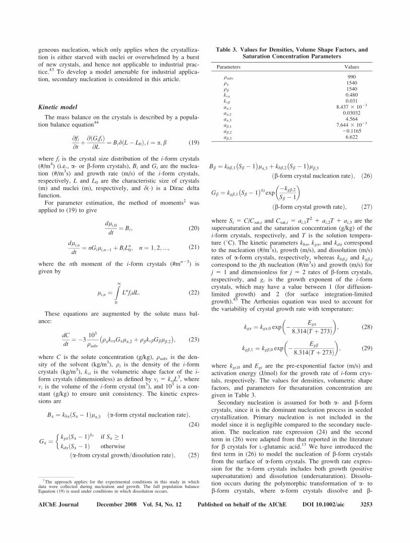
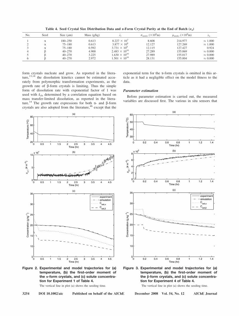
Figure 2. Experimental and model trajectories for (a)temperature, (b) the first-order moment ofthe a-form crystals, and (c) solute concentra-tion for Experiment 1 of Table 4.

The vertical line in plot (a) shows the seeding time.

Figure 3. Experimental and model trajectories for (a)temperature, (b) the first-order moment ofthe b-form crystals, and (c) solute concentra-tion for Experiment 4 of Table 4.



have become available for crystallization processes haveremoved or reduced sampling of the crystal slurry duringcrystallization and reduced the amount of pharmaceuticalneeded for each batch experiment. The two in situ measure-ments utilized in this study were ATR-FTIR spectroscopy,which infers the solute concentration and FBRM that pro-vides crystal size information throughout the batch. Inferen-tial modeling was used to construct a calibration curve torelate the FTIR spectra to the solute concentration, using pro-cedures described elsewhere.47,48 FBRM measures the chordlength distribution (CLD), which is not the same as the crys-tal size distribution (CSD) that appears in the models in theprevious section.

The CSD can be computed from the CLD under certainassumptions.49–52 For some systems, the square-weightedchord length was found to be comparable to laser diffraction,sieving, and electrical sensing zone analysis over the rangeof 50–400 lm.53 Although the aforementioned methods areable to estimate the CSD from CLD successfully for somesystems, the theory behind these methods require manyassumptions, including that the particles perfectly backscatterlight at all angles and that shape of the crystals is known.Although these assumptions are true for many particulatesystems (such as round polymer beads with a rough surfacein water at low-to-moderate solids densities52), the assump-tions are not accurate for other particulate systems includingthe system studied here which has crystals with a similar re-fractive index as the solution (and hence poor backscatteringproperties). Because of the limited time and pharmaceuticalquantity available in the early stage of batch crystallizationdesign, it is typically not possible to carry out the extensivestudies to verify the assumptions and to determine the effectsof nonideality of the assumptions on the accuracy of the esti-mates of the CSD from the CLD. Furthermore, computingthe CSD from the CLD when assumptions such as perfectlaser backscattering do not hold is still an open problem.51,54

Table 5. Definition of Measured Variables y and InterestedParameters h for a- and b-Seeded Experiments

Seed hT yT

a [ln(kba), ln(kga,0),ga, ln(Ega),ln(kbb,1), ln(rca), ln(rla,1), ln(rxa)]

[C, la,1, xa]

b [ln(kbb,2), ln(kgb,0), ln(kgb,2),gb, ln(Egb), ln(rcb), ln(rlb,1)]

[C, lb,1]

Figure 4. The marginal distributions of parameters h obtained from a-seeded experiments (Table 5).


An alternative approach is to use the low-order momentsof the CLD directly,54,55 without first estimating the CSDfrom the CLD. This approach replaces the first-principlesmodel for the CSD with a gray-box model for the CLD, inwhich the structure of the first-principles model for the low-order moments of the CSD is used to parametrize the low-order moments for the CLD.54 The reasoning behind this par-ticular gray-box model is that the mapping between the CLDand the CSD is static (most of the aforementioned mappingmethods assume that the mapping is actually linear), so thelow-order moments of the CLD should follow the samedynamic trends as the low-order moments of the CSD.Because of the limitation of the FBRM precision, the zerothmoment was not used because FBRM would undercount thevery small crystals. On the other hand, it is not advisable touse moments with order higher than two because higherorder moments are sensitive to low-sampling statistics of thelarge crystals.55 In this study, the first-order moment wasused. As with any model,25 this article assesses the applic-ability of this gray-box modeling by quantifying the accuracyof the kinetic parameters and the model’s predictions.

The experiments are categorized into two sets, namely,a-seeded and b-seeded experiments. The seed crystal size

distribution was approximated as a normal distribution

fi L; 0ð Þ ¼ fseed;i Lð Þ ¼ kiffiffiffiffiffiffi2p

prseed;i

exp �L� lseed;i

� �2

2r2seed;i

!;

(30)

with the parameters (ki, rseed,i, and lseed,i) in Table 4. Thetime series for the temperature, first-order moment of the i-

Table 6. The Model Parameters Determined fromParameter Estimation

Parameters Mean Mode 95% Credible Interval

ln(kba) 17.233 17.213 17.083–17.377ln(kga,0) 1.878 1.778 0.801–2.912ga 1.859 1.860 1.775–1.944ln(Ega) 10.671 10.671 10.612–10.725ln(kbb,1) 15.801 15.796 15.758–15.842ln(kbb,2) 20.000 20.000 19.961–20.036ln(kgb,0) 52.002 52.426 50.745–53.322ln(kgb,2) 20.251 20.251 20.311–20.197gb 1.047 1.016 1.002–1.143ln(Egb) 12.078 12.076 12.060–12.097

Figure 5. The marginal distributions of parameters h obtained from b-seeded experiments (Table 5).


form crystals, and solute concentration for Experiments 1and 4 are shown by the solid lines in Figures 2 and 3.§ Forall the b-seeded experiments, there is no apparent formationof a-form crystals at the end of all batches (Table 4).} As aresult, the kinetic parameters for b-form crystals were inde-pendently obtained from the b-seeded experiments, exceptfor kbb,1, which accounts for the nucleation of b-form a-formcrystals. One a-seeded experiment was operated at a highenough temperature that a measurable quantity of b-formcrystals nucleated and grew (Experiment 3 in Table 4), sothere would be enough information content in the data forkbb,1 to be estimated. This experimental design enabled thekinetic parameters for b-form crystals to be obtained beforedetermining the kinetic parameters for a-form crystals.

The nucleation and growth kinetics of a and b-form crys-tals have 10 parameters to be estimated, four (kba, kga,0, ga,Ega) corresponding to the kinetics of a-form crystals and six(kbb,1, kbb,2, kgb,0, kgb,2, gb, Egb) corresponding to the kineticsof b-form crystals. In relation to the notation defined in theReview of Bayesian Inference section, the measured varia-bles y and parameters of interest h for each set of experi-ments are defined in Table 5, where rci, rli,1

, rxi are thenoise parameters for the i-form crystals. The prior distribu-tion Pr(h) came from a preliminary parameter estimation thatwas carried out using maximum likelihood techniques asdescribed in Miller and Rawlings,23 which resulted in a nor-mal distribution for each parameter. These were modified forga and gb according to (4) to limit their values between 1and 2. The resulting marginal probability distributions of hfrom a- and b-seeded experiments are in Figures 4 and 5,respectively. While some of the marginal probability distribu-tions could be approximated by a normal distribution, othersare not. These distributions can be directly inserted into thosemodel predictive control and other control algorithms thathave been designed to ensure robustness to stochastic param-eter uncertainties.24 The means, modes, and 95% credibleintervals for the model parameters based on their marginalprobability distributions are in Table 6. Figures 2 and 3 com-pare the temperature, first-order moment of the a-form crys-tals, and solute concentration trajectories obtained from ex-perimental data and those predicted through simulation usingthe aforementioned mean values as the model parameters.

It is well known that concentration data alone are not suf-ficient to characterize nucleation.23 The small uncertainties inthe nucleation kinetic parameters indicate that the first-ordermoment of the FBRM provided enough information to char-acterize the nucleation kinetics. The small range in the uncer-tainties for the activation energies indicates that the tempera-ture range from 24 to 558C in the experiments was largeenough to enable activation energies to be estimated. The

rather large uncertainty in kga,0 is mainly due to the largecorrelation coefficient of 0.993 between kga,0 and Ega, wherea small change in Ega necessitates a larger change in kga,0 toensure the resulting kga in (28) is of the same order of mag-nitude. Similar reasoning explains the large uncertainty inkgb,0, with the correlation coefficient between kgb,0 and Egb

equal to 0.997. The growth exponent for the a-form is near2, which indicates that the a-form growth rate is surface inte-gration-limited, whereas that for the b-form is near 1, sug-gesting that the b-form growth rate is diffusion-limited.Unlike past studies that quantified uncertainties in the kinetic

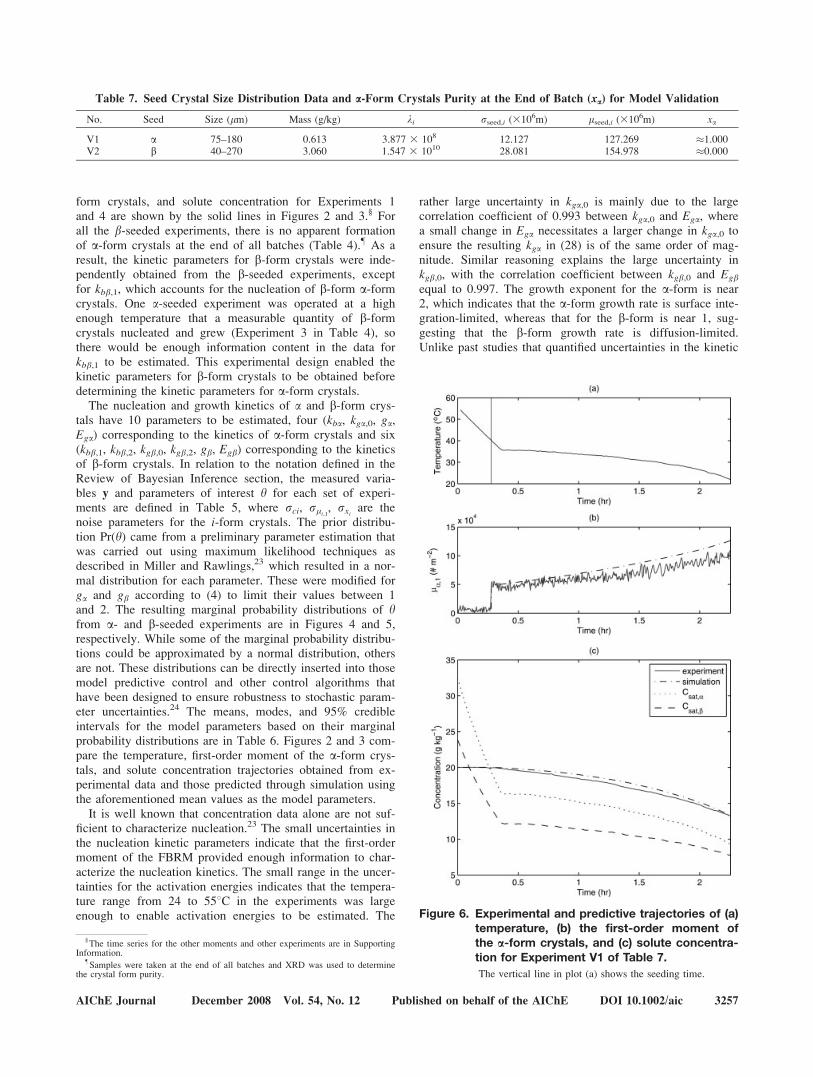
Table 7. Seed Crystal Size Distribution Data and a-Form Crystals Purity at the End of Batch (xa) for Model Validation

No. Seed Size (lm) Mass (g/kg) ki rseed,i (3106m) lseed,i (3106m) xa

V1 a 75–180 0.613 3.877 3 108 12.127 127.269 �1.000V2 b 40–270 3.060 1.547 3 1010 28.081 154.978 �0.000

Figure 6. Experimental and predictive trajectories of (a)temperature, (b) the first-order moment ofthe a-form crystals, and (c) solute concentra-tion for Experiment V1 of Table 7.


§The time series for the other moments and other experiments are in Supporting

Information.}Samples were taken at the end of all batches and XRD was used to determine

the crystal form purity.


parameters for crystallization processes,23,54 the analysis inthis article explicitly takes into account hard theoreticalbounds on the values for the parameters. In particular, theapplication of the linearized analyses used in past paperswould have resulted in a confidence interval that includedvalues of gb \ 1, whereas the Markov Chain simulationapproach takes the lower bound of 1 into account during thestatistical analysis (see Figure 5d).

To assess the predictive capability of the resulting model,another pair of experiments (i.e., one a- and one b-seededexperiment) were carried out with the seed distributions inTable 7. The trajectories of the temperature, first-ordermoment of the i-form crystals, and solute concentration tra-jectories obtained from experimental data and those predictedthrough simulation are plotted in Figures 6 and 7. As can beseen from these figures, the predictive capability of themodel is sufficiently accurate for use in process design andcontrol. The solute concentration predicted by the model are

quite close to the measured solute concentration in both vali-dation experiments, with the differences between the pre-dicted and experimental first-order moment being comparableto or smaller than the differences in the model and experi-mental first-order moments in the experiments used for pa-rameter estimation (compare Figures 6 and 7 with Figures 2and 3). The biases observed in the model predictions for thefirst-order moment of the i-form crystals could be due to theFBRM undercounting very small and large crystals, whichwould cause a different time-varying bias in different experi-ments.

Conclusions

A model of polymorphic crystallization of L-glutamic acid,which consist of a- and b-form crystallization, has beendeveloped. The detailed kinetics model takes into accountthe temperature dependence of the crystals growth kinetic pa-rameters when compared with the past studies on the model-ing of L-glutamic acid crystallization.13,14 In addition to pro-viding point estimates of the kinetic parameters, a Bayesianinference approach is used to determine a detailed marginalprobability distribution for each parameter. The marginalprobability distributions of the parameters can give practi-tioners insight regarding the parameter uncertainties and areof significant value to develop robust control strategies forthe crystallization process.24

Although this article considers a specific polymorphiccrystallization, the same parameter estimation method can beapplied for crystallizations in which many nucleation andgrowth rates occur simultaneously, or when there are no priorliterature data or estimates for the model parameters. Thedetails of the nucleation and growth rate expressions may bedifferent, depending on the particular solute–solvent system.With multiple polymorphs in the crystallizer, improved pa-rameter estimates would be obtained by including polymorphratio measurements obtained from in situ Raman spectros-copy in (3).56

Literature Cited

1. De Anda JC, Wang XZ, Lai X, Roberts KJ. Classifying organiccrystals via in-process image analysis and the use of monitoringcharts to follow polymorphic and morphological changes. J ProcessControl. 2005;15:785–797.

2. Blagden N, Davey R. Polymorphs take shape. Chem Britain.1999;35:44–47.

3. Fujiwara M, Nagy ZK, Chew JW, Braatz RD. First-principles anddirect design approaches for the control of pharmaceutical crystalli-zation. J Process Control. 2005;15:493–504.

4. Rohani S, Horne S, Murthy K. Control of product quality in batchcrystallization of pharmaceuticals and fine chemicals, Part 1: Designof the crystallization process and the effect of solvent. Org ProcessRes Dev. 2005;9:858–872.

5. Yu LX, Lionberger RA, Raw AS, D’Costa R, Wu HQ, Hussain AS.Applications of process analytical technology to crystallization proc-esses. Adv Drug Delivery Rev. 2004;56:349–369.

6. Cardew PT, Davey RJ. The kinetics of solvent-mediated phase trans-formations. Proc R Soc Lond A. 1985;398:415–428.

7. Sakai H, Hosogai H, Kawakita T, Onuma K, Tsukamoto K. Transfor-mation of a-glycine to c-glycine. J Cryst Growth. 1992;116:421–426.

8. Saranteas K, Bakale R, Hong YP, Luong H, Foroughi R, Wald S.Process design and scale-up elements for solvent mediated polymor-phic controlled tecastemizole crystallization. Org Process Res Dev.2005;9:911–922.

Figure 7. Experimental and predictive trajectories of (a)temperature, (b) the first-order moment ofthe b-form crystals, and (c) solute concentra-tion for Experiment V2 of Table 7.



9. Yu L. Survival of the fittest polymorph: how fast nucleater can loseto fast grower. CrystEngComm. 2007;9:841–851.

10. Bard Y. Nonlinear Parameter Estimation. New York: AcademicPress. 1974.

11. Bates DM, Watts DG. Nonlinear Regression Analysis and Its Appli-cations. New York: Wiley, 1988.

12. Mendes P, Kell DB. Non-linear optimization of biochemical path-ways: applications to metabolic engineering and parameter estima-tion. Bioinformatics. 1998;14:869–883.

13. Ono T, Kramer HJM, Ter Horst JH, Jansens PJ. Process modeling ofthe polymorphic transformation of L-glutamic acid. Cryst GrowthDes. 2004;4:1161–1167.

14. Scholl J, Bonalumi D, Vicum L, Mazzotti M. In situ monitoring andmodeling of the solvent-mediated polymorphic transformation ofL-Glutamic acid. Cryst Growth Des. 2006;6:881–891.

15. Caillet A, Sheibat-Othman N, Fevotte G. Crystallization of monohy-drate citric acid. II. Modeling through population balance equations.Cryst Growth Des. 2007;7:2088–2095.

16. Fevotte G, Alexandre C, Nida SO. A population balance model ofthe solution-mediated phase transition of citric acid. AIChE J.2007;53:2578–2589.

17. Box GEP, Draper NR. The Bayesian estimation of common parame-ters from several responses. Biometrika. 1965;52:355–365.

18. Duran MA, White BS. Bayesian estimation applied to effective heattransfer coefficients in a packed bed. Chem Eng Sci. 1995;50:495–510.

19. Bois FY, Fahmy T, Block JC, Gatel D. Dynamic modeling of bacte-ria in a pilot drinking-water distribution system. Water Res. 1997;31:3146–3456.

20. Coleman MC, Block DE. Bayesian parameter estimation with in-formative priors for nonlinear systems. AIChE J. 2006;52:651–667.

21. Pouillot R, Albert I, Cornu M, Denis JB. Estimation of uncertainty andvariability in bacterial growth using Bayesian inference. Applicationto listeria monocytogenes. Int J Food Microbiol. 2003;81:87–104.

22. Gunawan R, Jung MY, Seebauer EG, Braatz RD. Maximum a poste-riori estimation of transient enhanced diffusion energetics. AIChE J.2003;49:2114–2122.

23. Miller SM, Rawlings JB. Model identification and control strategiesfor batch cooling crystallizers. AIChE J. 1994;40:1312–1327.

24. Nagy ZK, Braatz RD. Worst-case and distributional robustness analy-sis of finite-time control trajectories for nonlinear distributed parame-ter systems. IEEE Trans Control Syst Technol. 2003;11:694–704.

25. Beck JV, Arnold KJ. Parameter Estimation in Engineering and sci-ence. New York: Wiley, 1977.

26. Tierney L. Markov Chains for exploring posterior distributions. AnnStat. 1994;22:1701–1728.

27. Liu JS. Monte Carlo Strategies in Scientific Computing. New York:Springer, 2001.

28. Gelman A, Carlin JB, Stern HS, Rubin DB. Bayesian Data Analysis.New York: Chapman & Hall/CRC, 2004.

29. Chen WS, Bakshi BR, Goel PK, Ungarala S. Bayesian estimationvia sequential Monte Carlo sampling: unconstrained nonlineardynamic systems. Ind Eng Chem Res. 2004;43:4012–4025.

30. Lang L, Chen WS, Bakshi BR, Goel PK, Ungarala S. Bayesian esti-mation via sequential Monte Carlo sampling - constrained dynamicsystems. Automatica. 2007;43:1615–1622.

31. Fujiwara M, Chow PS, Ma DL, Braatz RD. Paracetamol crystalliza-tion using laser backscattering and ATR-FTIR spectroscopy: meta-stability, agglomeration and control. Cryst Growth Des. 2002;2:363–370.

32. Togkalidou T, Fujiwara M, Patel S, Braatz RD. Solute concentrationprediction using chemometrics and ATR-FTIR spectroscopy. J CrystGrowth. 2001;231:534–543.

33. Xie YL, Kalivas JH. Evaluation of principal component selectionmethods to form a global prediction model by principal componentregression. Anal Chim Acta. 1997;348:19–27.

34. Bretthorst GL. An introduction to parameter estimation using Bayes-ian probability theory. In: Fougere PF, editor. Maximum Entropy andBayesian Methods. Dordrecht: Kluwer Academic Publishers,1990:53–79.

35. Carlin BP, Louis TA. Bayes and Empirical Bayes Methods for DataAnalysis. Boca Raton: Chapman & Hall/CRC, 2000.

36. Box GEP, Tiao GC. Bayesian Inference in Statistical Analysis.Reading, Mass: Addison-Wesley, 1973.

37. Metropolis N, Rosenbluth AW, Rosenbluth MN, Teller AH. Equa-tion of state calculations by fast computing machines. J Chem Phys.1953;21:1087–1092.

38. Haario H, Saksman E, Tamminen J. An adaptive Metropolis algo-rithm. Bernoulli. 2001;7:223–242.

39. Liang FM, Wong WH. Real-parameter evolutionary Monte Carlowith applications to Bayesian mixture models. J Am Stat Assoc.2001;96:653–666.

40. Liang F. Dynamically weighted importance sampling in Monte Carlocomputation. J Am Stat Assoc. 2002;97:807–821.

41. Laskey KB, Myers JW. Population Markov Chain Monte Carlo.Machine Learn. 2003;50:175–196.

42. Braak CJ. A Markov Chain Monte Carlo version of the genetic algo-rithm differential evolution: easy Bayesian computing for real pa-rameter spaces. Stat Comput. 2006;16:239–249.

43. Clontz NA, McCabe WL. Contact nucleation of magnesium sulfateheptahydrate. AIChE Symp Ser. 1971;67:6–17.

44. Hulburt HM, Katz S. Some problems in particle technology: a statis-tical mechanical formulation. Chem Eng Sci. 1964;19:555–574.

45. Mersmann A. Crystallization Technology Handbook, 2nd ed. BocaRaton: CRC Press, 2001.

46. Kitamura M, Ishizu T. Growth kinetics and morphological change ofpolymorphs of L-glutamic acid. J Cryst Growth. 2000;209:138–145.

47. Togkalidou T, Braatz RD, Johnson B, Davidson O, Andrews A. Ex-perimental design and inferential modeling in pharmaceutical crys-tallization. AIChE J. 2001;47:160–168.

48. Togkalidou T, Tung HH, Sun Y, Andrews A, Braatz RD. Solutionconcentration prediction for pharmaceutical crystallization processesusing robust chemometrics and ATR FTIR spectroscopy. Org Pro-cess Res Dev. 2002;6:317–322.

49. Tadayyon A, Rohani S. Determination of particle size distributionby Par-Tec 100: modeling and experimental results. Part Part SystCharact. 1998;15:127–135.

50. Simmons M, Langston P, Burbidge A. Particle and droplet size anal-ysis from chord distributions. Powder Technol. 1999;102:75–83.

51. Ruf A, Worlitschek J, Mazzotti M. Modeling and experimental anal-ysis of PSD measurements through FBRM. Part Part Syst Charact.2000;17:167–179.

52. Hukkanen EJ, Braatz RD. Measurement of particle size distributionin suspension polymerization using in situ laser backscattering. SensActuators B. 2003;96:451–459.

53. Heath AR, Fawell PD, Bahri PA, Swift JD. Estimating average parti-cle size by focused beam reflectance measurement (FBRM). PartPart Syst Charact. 2002;19:84–95.

54. Togkalidou T, Tung HH, Sun Y, Andrews AT, Braatz RD. Parame-ter estimation and optimization of a loosely-bound aggregating phar-maceutical crystallization using in-situ infrared and laser backscatter-ing measurements. Ind Eng Chem Res. 2004;43:6168–6181.

55. Gunawan R, Ma DL, Fujiwara M, Braatz RD. Identification of ki-netic parameters in a multidimensional crystallization process. Int JMod Phys B. 2002;16:367–374.

56. Starbuck C, Spartalis A, Wai L, Wang J, Fernandez P, LindemannCM, Zhou GX, Ge ZH. Process optimization of a complex pharma-ceutical polymorphic system via in situ Raman spectroscopy. CrystGrowth Des. 2002;2:515–522.

Manuscript received Jan. 14, 2008, and revision received July 8, 2008.


Documents

Robust Bayesian Estimation of Kinetics for the Polymorphic ...web.mit.edu/braatzgroup/Robust_Bayesian_estimation_of_the_kinetics... · Robust Bayesian Estimation of Kinetics for the