The debate on the effects of fiscal consolidations

Roberto Perotti

IGIER – Bocconi University, CEPR and NBER

December 2013

Many European countries have high levels of public debt, and are going through periods of budget

austerity. Many economists and policymakers fear that these austerity programs might exacerbate the

recession; others argue that properly designed austerity programs can even be expansionary. This essay is in

two parts. I briefly review what we know about the likely effects of these fiscal consolidations.

Fiscal consolidations: the mean comparison approach

A first method to investigate the effects of a fiscal consolidation is simply to extrapolate from current

estimates of tax and spending multipliers, from time series Vector Autoregression studies. There are several

recent surveys of existing results, mostly based on US data. Therefore, I will concentrate on studies that focus

explicitly on episodes of fiscal consolidations.

Focusing especially on fiscal consolidations introduces a larger cross country set of events; it is also

useful if nonlinearities are important, and the results depend on the size of the initial government debt or

deficit, the size of the fiscal adjustment, or even less easily defined things like the “sense of crisis”.

Two statistical approaches have been used to study large fiscal consolidations. The first consists of a

simple comparison of means of variables over time. Specifically: (i) define a “fiscal consolidation”, for instance

as a country-year when the discretionary 1 decline in the primary deficit is more than, say, 1.5 percent of GDP,

1 The “discretionary” change in the deficit is that part of the change in the deficit that is not due to the automatic response of the deficit to the economic cycle. In this sense, it can be interpreted as the part of the change in the deficit that is due to intentional actions by the policymakers, like changes in tax rates, in replacement rate for unemployment benefits, in defense spending etc. The same definition applies to each individual budget component.

1

or two consecutive country-years when it is at least 1 percent each year; (ii) take a macroeconomic variable of

interest, like private consumption, and compare the average of that variable in the two years after (or during)

the consolidation with the average in the two years before the consolidation. This “mean comparison”

approach would provide unbiased estimates of the average effects of consolidations if the latter were

completely random events (in which case it is essentially a difference – in – difference estimator).

This is the methodology applied by Alesina and Perotti (1995) and Alesina and Ardagna (2010) with

cyclically adjusted data, and by Alesina and Ardagna (2012) with the narrative IMF data of Devries et al.

(2011).2 The typical result is that spending-based consolidations (where the discretionary decline in the

deficit consists of at least 50 percent spending cuts) tend to be longer-lasting and are associated with an

increase in GDP growth or a small recession, while tax-based consolidations are short-lived and are associated

with a slowdown in growth or even a recession. With some variations, all of private consumption, investment,

and exports display this pattern. Also, in general these variables are particularly responsive to cuts in social

spending or spending on public wages and salaries – the two largest government spending items in all OECD

countries.

Fiscal consolidations are typically multi-year events. In this methodology, a fiscal consolidation lasting

four years would appear as three consecutive two-year consolidations; moreover, a given year can appear in

all of the “pre”, “during” and “post” groups at different dates. It is not clear what the “mean comparison”

method delivers in these cases.

A second problem with this approach is that it is difficult to control for concomitant effects. For

instance, one typical result is that spending-based consolidations are associated with real depreciation of the

2 There are two methods to obtain “discretionary” measures of a change in a budget variable. First, the “cyclical adjustment” method: estimate the elasticities of that budget variable to, say, output and inflation, and subtract from the actual change in the budget variable the change in output multiplied by the output elasticity and the change in inflation multiplied by the inflation elasticity. Second, the “narrative” method, pioneered by Romer and Romer (2010) for revenues changes: use budget documents to infer the discretionary change in tax revenues or spending enacted by any law that has consequences for the budget. Devries et al. (2011) compute yearly discretionary changes in government spending and revenues during periods of deficit reductions in 15 countries.

2

exchange rate and improvement in relative unit labor costs. Is this a consequence of spending-based

consolidations, or is this the result of policies typically implemented together with spending based

consolidations? As always, causality is difficult to ascertain.

The accompanying policies might take several forms which might be difficult to capture with one or

two variables: consider for instance labor market reforms, or changes in exchange rate or monetary policy

regimes. Finally, the government budgets and accompanying technical documents need to be studied in

depth in order to determine the discretionary measures with a minimum of confidence.

Fiscal consolidations: case studies

For all these reasons, it is useful to complement the existing evidence with a different approach.

Perotti (2012) presents a detailed discussion of the four largest spending-based consolidations - Denmark

1983-87, Ireland 1987-89, Finland 1992-96, Sweden 1993-97 - based on the original budget documents and on

contemporary discussion, like OECD or IMF annual reports, and country-specific sources.3 I focus on two

questions. First, is there evidence that large budget consolidations can have expansionary effects in the short

run? Second, how useful is the experience of the past as a guide to today’s Eurozone countries?

The main conclusions of the case studies I present are:

(i) Actual consolidations were smaller than previously thought, and not spending-based. All these

consolidations have long been considered quintessential cases of large, “spending-based consolidations”. Two

of these were truly enormous: as shown in Table 1, columns 3 and 6, in Finland the discretionary primary

deficit fell by 11.5 percent of GDP over 5 years (all of them spending cuts) , according to the IMF narrative

measure of Devries et al. (2011), and in Sweden by 10.6 percent of GDP over 5 years (of which almost 7 pps of

GDP spending cuts).

3 The pros and cons of case studies vs. an econometric approach are well known. Hence, I will not revisit this debate here.

3

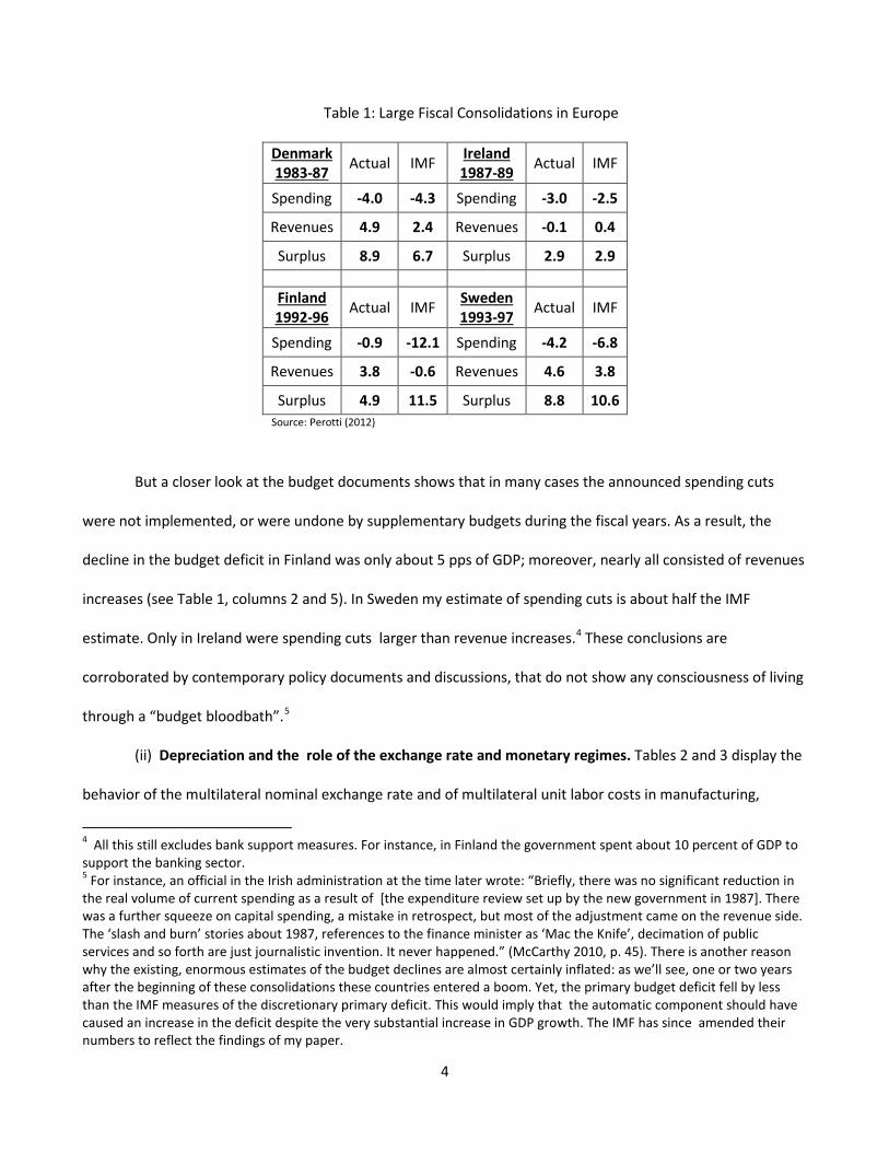
Table 1: Large Fiscal Consolidations in Europe

Denmark 1983-87 Actual IMF Ireland

1987-89 Actual IMF

Spending -4.0 -4.3 Spending -3.0 -2.5

Revenues 4.9 2.4 Revenues -0.1 0.4

Surplus 8.9 6.7 Surplus 2.9 2.9

Finland 1992-96 Actual IMF Sweden

1993-97 Actual IMF

Spending -0.9 -12.1 Spending -4.2 -6.8

Revenues 3.8 -0.6 Revenues 4.6 3.8

Surplus 4.9 11.5 Surplus 8.8 10.6 Source: Perotti (2012)

But a closer look at the budget documents shows that in many cases the announced spending cuts

were not implemented, or were undone by supplementary budgets during the fiscal years. As a result, the

decline in the budget deficit in Finland was only about 5 pps of GDP; moreover, nearly all consisted of revenues

increases (see Table 1, columns 2 and 5). In Sweden my estimate of spending cuts is about half the IMF

estimate. Only in Ireland were spending cuts larger than revenue increases.4 These conclusions are

corroborated by contemporary policy documents and discussions, that do not show any consciousness of living

through a “budget bloodbath”.5

(ii) Depreciation and the role of the exchange rate and monetary regimes. Tables 2 and 3 display the

behavior of the multilateral nominal exchange rate and of multilateral unit labor costs in manufacturing,

4 All this still excludes bank support measures. For instance, in Finland the government spent about 10 percent of GDP to support the banking sector. 5 For instance, an official in the Irish administration at the time later wrote: “Briefly, there was no significant reduction in the real volume of current spending as a result of [the expenditure review set up by the new government in 1987]. There was a further squeeze on capital spending, a mistake in retrospect, but most of the adjustment came on the revenue side. The ‘slash and burn’ stories about 1987, references to the finance minister as ‘Mac the Knife’, decimation of public services and so forth are just journalistic invention. It never happened.” (McCarthy 2010, p. 45). There is another reason why the existing, enormous estimates of the budget declines are almost certainly inflated: as we’ll see, one or two years after the beginning of these consolidations these countries entered a boom. Yet, the primary budget deficit fell by less than the IMF measures of the discretionary primary deficit. This would imply that the automatic component should have caused an increase in the deficit despite the very substantial increase in GDP growth. The IMF has since amended their numbers to reflect the findings of my paper.

4

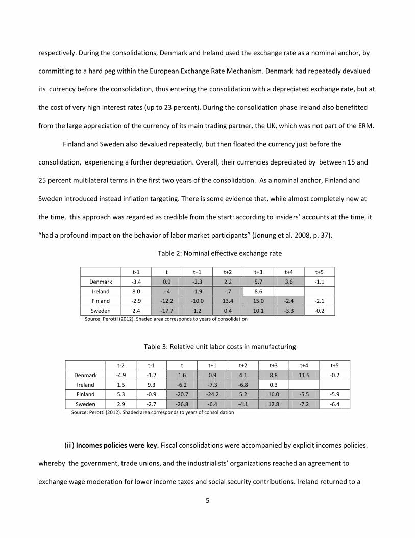
respectively. During the consolidations, Denmark and Ireland used the exchange rate as a nominal anchor, by

committing to a hard peg within the European Exchange Rate Mechanism. Denmark had repeatedly devalued

its currency before the consolidation, thus entering the consolidation with a depreciated exchange rate, but at

the cost of very high interest rates (up to 23 percent). During the consolidation phase Ireland also benefitted

from the large appreciation of the currency of its main trading partner, the UK, which was not part of the ERM.

Finland and Sweden also devalued repeatedly, but then floated the currency just before the

consolidation, experiencing a further depreciation. Overall, their currencies depreciated by between 15 and

25 percent multilateral terms in the first two years of the consolidation. As a nominal anchor, Finland and

Sweden introduced instead inflation targeting. There is some evidence that, while almost completely new at

the time, this approach was regarded as credible from the start: according to insiders’ accounts at the time, it

“had a profound impact on the behavior of labor market participants” (Jonung et al. 2008, p. 37).

Table 2: Nominal effective exchange rate

t-1 t t+1 t+2 t+3 t+4 t+5 Denmark -3.4 0.9 -2.3 2.2 5.7 3.6 -1.1

Ireland 8.0 -.4 -1.9 -.7 8.6 Finland -2.9 -12.2 -10.0 13.4 15.0 -2.4 -2.1 Sweden 2.4 -17.7 1.2 0.4 10.1 -3.3 -0.2

Source: Perotti (2012). Shaded area corresponds to years of consolidation

Table 3: Relative unit labor costs in manufacturing

t-2 t-1 t t+1 t+2 t+3 t+4 t+5 Denmark -4.9 -1.2 1.6 0.9 4.1 8.8 11.5 -0.2

Ireland 1.5 9.3 -6.2 -7.3 -6.8 0.3 Finland 5.3 -0.9 -20.7 -24.2 5.2 16.0 -5.5 -5.9 Sweden 2.9 -2.7 -26.8 -6.4 -4.1 12.8 -7.2 -6.4

Source: Perotti (2012). Shaded area corresponds to years of consolidation

(iii) Incomes policies were key. Fiscal consolidations were accompanied by explicit incomes policies.

whereby the government, trade unions, and the industrialists’ organizations reached an agreement to

exchange wage moderation for lower income taxes and social security contributions. Ireland returned to a

5

tripartite wage settlement in 1987 (see Table 3), which set a maximum increase in wages by 2.5 percent in

1988, 1989 and 1990. Finland and Sweden signed tripartite wage agreements at the start of the consolidations,

and then, after some wage slippage three years into the consolidation (see Table 3), the government

summoned the unions and industrialists’ association again to sign other wage agreements. These

developments were regarded as very significant by contemporaries: as Jonung, Kiander and Vartia (2008) write,

based on contemporary accounts, “perhaps the biggest change in the 1990’s in Finland was the adoption and

wide acceptance of a policy of long term wage moderation” (p. 35).

Incomes policies were particularly explicit in Denmark. Here, the government renounced any

depreciation of the exchange rate and relied instead on an internal devaluation: it suspended wage indexation,

capped contractual wage increases, froze unemployment subsidies and transfers, all in exchange for lower

income taxes and social security contributions.

Wage moderation, that was made possible by incomes policies, was instrumental in maintaining the

benefits of the nominal depreciations and in reducing inflation expectations and interest rates.

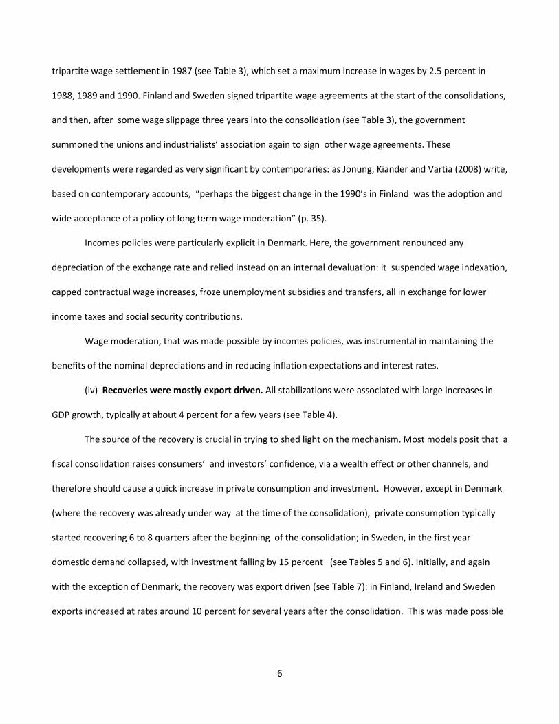
(iv) Recoveries were mostly export driven. All stabilizations were associated with large increases in

GDP growth, typically at about 4 percent for a few years (see Table 4).

The source of the recovery is crucial in trying to shed light on the mechanism. Most models posit that a

fiscal consolidation raises consumers’ and investors’ confidence, via a wealth effect or other channels, and

therefore should cause a quick increase in private consumption and investment. However, except in Denmark

(where the recovery was already under way at the time of the consolidation), private consumption typically

started recovering 6 to 8 quarters after the beginning of the consolidation; in Sweden, in the first year

domestic demand collapsed, with investment falling by 15 percent (see Tables 5 and 6). Initially, and again

with the exception of Denmark, the recovery was export driven (see Table 7): in Finland, Ireland and Sweden

exports increased at rates around 10 percent for several years after the consolidation. This was made possible

6

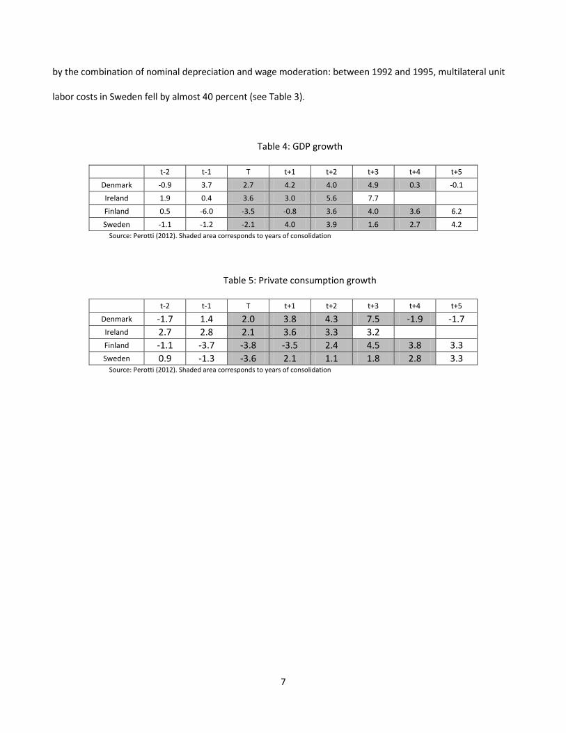
by the combination of nominal depreciation and wage moderation: between 1992 and 1995, multilateral unit

labor costs in Sweden fell by almost 40 percent (see Table 3).

Table 4: GDP growth

t-2 t-1 T t+1 t+2 t+3 t+4 t+5

Denmark -0.9 3.7 2.7 4.2 4.0 4.9 0.3 -0.1 Ireland 1.9 0.4 3.6 3.0 5.6 7.7 Finland 0.5 -6.0 -3.5 -0.8 3.6 4.0 3.6 6.2

Sweden -1.1 -1.2 -2.1 4.0 3.9 1.6 2.7 4.2 Source: Perotti (2012). Shaded area corresponds to years of consolidation

Table 5: Private consumption growth

t-2 t-1 T t+1 t+2 t+3 t+4 t+5 Denmark -1.7 1.4 2.0 3.8 4.3 7.5 -1.9 -1.7 Ireland 2.7 2.8 2.1 3.6 3.3 3.2 Finland -1.1 -3.7 -3.8 -3.5 2.4 4.5 3.8 3.3 Sweden 0.9 -1.3 -3.6 2.1 1.1 1.8 2.8 3.3

Source: Perotti (2012). Shaded area corresponds to years of consolidation

7

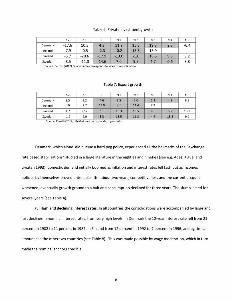
Table 6: Private investment growth

t-2 t-1 T t+1 t+2 t+3 t+4 t+5 Denmark -17.6 10.3 4.3 11.2 15.3 19.3 2.3 -6.4 Ireland -7.9 -0.5 -2.3 -0.2 13.5 13.9 Finland -5.7 -20.6 -17.9 -13.0 -1.6 18.5 9.3 9.2 Sweden -8.5 -11.3 -14.6 7.0 9.9 4.7 0.6 8.8

Source: Perotti (2012). Shaded area corresponds to years of consolidation

Table 7: Export growth

t-2 t-1 T t+1 t+2 t+3 t+4 t+5

Denmark 8.5 3.2 4.6 3.5 6.0 1.3 4.9 8.8 Ireland 6.6 2.7 13.9 8.1 11.4 9.2 Finland 1.7 -7.2 10 16.3 13.5 8.5 5.9 13.9

Sweden -1.9 2.0 8.3 13.5 11.3 4.4 13.8 9.0 Source: Perotti (2012). Shaded area corresponds to years of c

Denmark, which alone did pursue a hard peg policy, experienced all the hallmarks of the “exchange

rate based stabilizations” studied in a large literature in the eighties and nineties (see e.g. Ades, Kiguel and

Liviatan 1993): domestic demand initially boomed as inflation and interest rates fell fast; but as incomes

policies by themselves proved untenable after about two years, competitiveness and the current account

worsened; eventually growth ground to a halt and consumption declined for three years. The slump lasted for

several years (see Table 4).

(v) High and declining interest rates. In all countries the consolidations were accompanied by large and

fast declines in nominal interest rates, from very high levels. In Denmark the 10-year interest rate fell from 21

percent in 1982 to 11 percent in 1987, in Finland from 12 percent in 1992 to 7 percent in 1996, and by similar

amount s in the other two countries (see Table 8). This was made possible by wage moderation, which in turn

made the nominal anchors credible.

8

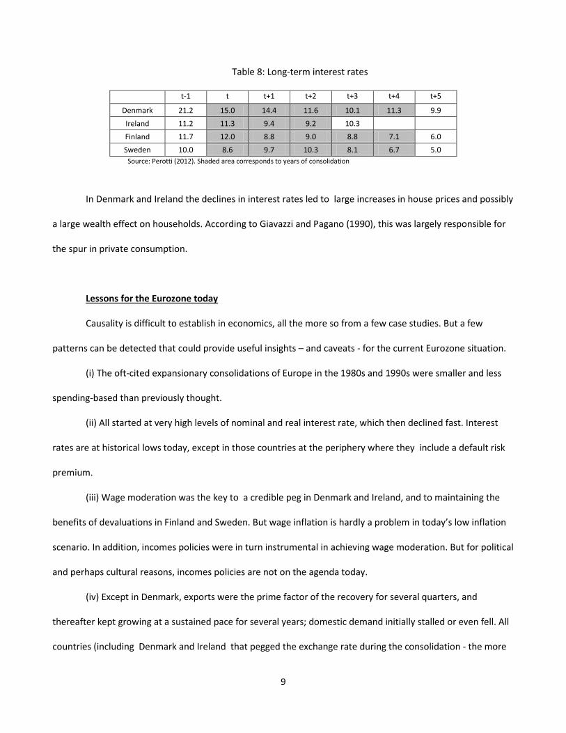
Table 8: Long-term interest rates

t-1 t t+1 t+2 t+3 t+4 t+5

Denmark 21.2 15.0 14.4 11.6 10.1 11.3 9.9

Ireland 11.2 11.3 9.4 9.2 10.3

Finland 11.7 12.0 8.8 9.0 8.8 7.1 6.0 Sweden 10.0 8.6 9.7 10.3 8.1 6.7 5.0

Source: Perotti (2012). Shaded area corresponds to years of consolidation

In Denmark and Ireland the declines in interest rates led to large increases in house prices and possibly

a large wealth effect on households. According to Giavazzi and Pagano (1990), this was largely responsible for

the spur in private consumption.

Lessons for the Eurozone today

Causality is difficult to establish in economics, all the more so from a few case studies. But a few

patterns can be detected that could provide useful insights – and caveats - for the current Eurozone situation.

(i) The oft-cited expansionary consolidations of Europe in the 1980s and 1990s were smaller and less

spending-based than previously thought.

(ii) All started at very high levels of nominal and real interest rate, which then declined fast. Interest

rates are at historical lows today, except in those countries at the periphery where they include a default risk

premium.

(iii) Wage moderation was the key to a credible peg in Denmark and Ireland, and to maintaining the

benefits of devaluations in Finland and Sweden. But wage inflation is hardly a problem in today’s low inflation

scenario. In addition, incomes policies were in turn instrumental in achieving wage moderation. But for political

and perhaps cultural reasons, incomes policies are not on the agenda today.

(iv) Except in Denmark, exports were the prime factor of the recovery for several quarters, and

thereafter kept growing at a sustained pace for several years; domestic demand initially stalled or even fell. All

countries (including Denmark and Ireland that pegged the exchange rate during the consolidation - the more

9

relevant case for today’s Eurozone members) devalued repeatedly before the consolidations. This option is

obviously not available to Eurozone members, except vis-à-vis non-Eurozone members. Ireland also benefitted

from the appreciation of the currency of its main trading partner, the UK. On the other hand, the Danish

expansion was short lived, as it quickly ran into a loss of competitiveness that hampered growth for several

years.

In this paper, I do not want to enter the debate of whether fiscal austerity is needed, how much, and

where. But the observations above suggest that the notion of “expansionary fiscal austerity” in the short run is

probably an illusion: a trade-off does seem to exist between fiscal austerity and short-run growth.

10

References

Ades, A., M. Kiguel, and N. Liviatan (1993): “Exchange-rate-based stabilization: Tales from Europe and Latin America”, World Bank Policy Research Working Paper WPS 1087

Alesina, A. and S. Ardagna (2010): “Large Changes in Fiscal Policy: Taxes versus Spending,” in: Tax Policy and the Economy, Vol. 24, ed. By Jeffrey R. Brown (Cambridge, Massachusetts: National .Bureau of Economic Research)

Alesina, A. and S. Ardagna (2012): “The Design of Fiscal Adjustments”, mimeo, Bocconi University Alesina, A. and R. Perotti (1995): “Fiscal Expansions and Adjustments in OECD Economies”, Economic Policy,

n.21, 207-247. Brunnermeier, M. et al. (2011); “European Safe Bonds (ESBies)”, The Euro-nomics group, September 30, 2011 Calvo, G. (1988): “Servicing the Public debt: The Role of Expectations”, American Economic Review, Vol. 78, No.

4 (Sep., 1988), pp. 647-661 Claessens, S., A. Mody and S. Vallée (2012): “Paths to Eurobonds”, IMF working paper WP/12/172 Committee on the Global Financial System (CGFS) (2011): “ The Impact of sovereign credit risk on bank funding

conditions”, CGFS papers No 43, July 2011 Cotterill, Joseph (2012): “Seniority, the SMP, and the OMT”, FT Alphaville, September 6, 2012

http://ftalphaville.ft.com/2012/09/06/1148941/seniority-the-smp-and-the-omt/ Delpla, J. and j. von Weizsäcker (2011): “The Blue Bond Proposal”, Bruegel Policy Brief, updated version March

2011. Devries, P., J. Guajardo, D. Leigh, and A. Pescatori (2011): “A New Action-Based Dataset of Fiscal

Consolidation,”, IMF Working Paper No. 11/128. Data set available at www.imf.org/external/pubs/cat/longres.aspx?sk=24892.0

Eurostat (2011): “The statistical recording of operations undertaken by the European Financial Stability Facility”, Eurostat news release 13/2011, January 27, 2011

Giavazzi, F and M. Pagano (1990) ”Can Severe Fiscal Contractions Be Expansionary? Tales of Two Small European Countries", NBER Macroeconomics Annual 1990, Volume 5, pages 75-122 National Bureau of Economic Research, Inc.

Gros, D. (2013): “Banking Union with a Sovereign Virus”, CEPS Policy Brief No 289, March 2013 Jonung, L., J. Kiander, and P. Vartia (2008): ”The great financial crisis in Finland and Sweden”, Economic Paper,

DG ECFIN McCarthy, C. (2010): “Ireland’s second round of cuts: a comparison with the last time”, in: Springford, J.:

Dealing with debt: lessons from abroad, CentreForum Canada, Ernst & Young, 41-54 Merler, S. and and J Pisani-Ferry (2012): "Who's afraid of sovereign bonds" , Bruegel Policy Contribution

2012|02, February Perotti R. (2012) "The Austerity Myth: "Growth without Pain?", forthcoming in A. Alesina and F. Giavazzi (eds.)

Fiscal Policy After the Great Recession University of Chicago Press and NBER. Pisani-Ferry, J. and G. Wolff (2012): "Propping up Europe?" , Bruegel Policy Contribution 2012|07, April Romer, C. and D. Romer (2010): “The Macroeconomic Effects of Tax Changes: Estimates Based on a New

Measure of Fiscal Shocks,” American Economic Review, Vol. 100, No. 3, pp. 763-801. Tirole, J. (2012): “Country solidarity, private sector involvement, and the contagion of sovereign crises”,

mimeo, University of Toulouse.

11

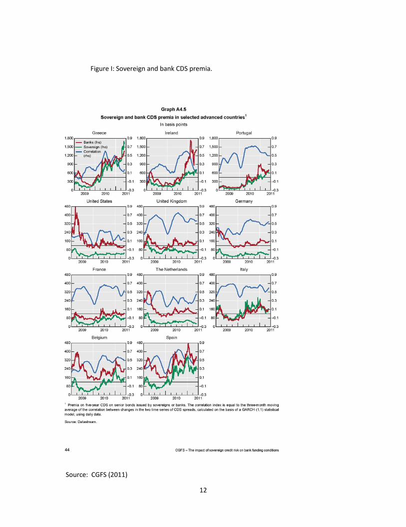
Figure I: Sovereign and bank CDS premia.

Source: CGFS (2011)

12

NBER WORKING PAPER SERIES

LARGE CHANGES IN FISCAL POLICY:TAXES VERSUS SPENDING

Alberto F. AlesinaSilvia Ardagna

Working Paper 15438http://www.nber.org/papers/w15438

NATIONAL BUREAU OF ECONOMIC RESEARCH1050 Massachusetts Avenue

Cambridge, MA 02138October 2009

Prepared for Tax Policy and the Economy 2009. We thank Jeffrey Brown, Roberto Perotti, MatthewShapiro and other conference participants for useful comments and discussions. The views expressedherein are those of the author(s) and do not necessarily reflect the views of the National Bureau ofEconomic Research.

© 2009 by Alberto F. Alesina and Silvia Ardagna. All rights reserved. Short sections of text, not toexceed two paragraphs, may be quoted without explicit permission provided that full credit, including© notice, is given to the source.

Large Changes in Fiscal Policy: Taxes Versus SpendingAlberto F. Alesina and Silvia ArdagnaNBER Working Paper No. 15438October 2009, Revised January 2010JEL No. H2,H3

ABSTRACT

We examine the evidence on episodes of large stances in fiscal policy, both in cases of fiscal stimuliand in that of fiscal adjustments in OECD countries from 1970 to 2007. Fiscal stimuli based upontax cuts are more likely to increase growth than those based upon spending increases. As for fiscaladjustments, those based upon spending cuts and no tax increases are more likely to reduce deficitsand debt over GDP ratios than those based upon tax increases. In addition, adjustments on the spendingside rather than on the tax side are less likely to create recessions. We confirm these results with simpleregression analysis.

Alberto F. AlesinaDepartment of EconomicsHarvard UniversityLittauer Center 210Cambridge, MA 02138and NBERaalesina@harvard.edu

Silvia ArdagnaDepartment of EconomicsHarvard UniversityLittauer CenterCambridge, MA 02138sardagna@fas.harvard.edu

1 Introduction

As a result of the fiscal response to the financial crisis of 2007-2009 the US willexperience the largest increases in deficits and debt accumulation in peacetime.Virtually all other OECD countries will also face fiscal imbalances of various sizes.After the large reduction in government deficits of the nineties and early new cen-tury, public finances in the OECD are back in the deep red.

Only a few months ago the key policy question was whether tax cuts or spend-ing increases were a better recipe for the stimulus plan in the US and other countriesas well. By and large these decisions have been taken, and we are in the processof observing the results. The next question which governments all over the worldwill face next year, assuming, as it seems likely, that a recovery next year will beunder way, is how to stop the growth of debt and return to more “normal” publicfinances.

The first question, namely whether tax cuts or spending increases are moreexpansionary is a critical one, and economists strongly disagree about the answer.It is fair to say that we know relatively little about the effect of fiscal policy ongrowth and in particular about the so called fiscal multipliers, namely how muchone dollar of tax cuts or spending increases translates in terms of GDP. The issue isvery politically charged as well, since right of center economists and policymakersbelieve in tax cuts and the left of center ones believe in spending increases. Whilethe differences are often rooted in different views about the role of government andinequality, not so much about the size of fiscal multipliers, both sides also wishto "sell" their prescription as growth enhancing and more so than the other policy.Unfortunately both sides can’t be right at the same time!

As far as reduction of large public debts the lesson from history is reasonablyoptimistic. Large debt/GDP ratios have been cut relatively rapidly by sustainedgrowth. This was the case of post WWII public debts in belligerent countries; itwas also the case of the US in the nineties when without virtually any increase intax rates or significant spending cuts, a large deficit turned in a large surplus.1 Inthe UK the debt over GDP ratio at the end of WWII was over 200 percent but thatcountry did not suffer a financial crisis due to its historically credible fiscal stanceand the debt was gradually and relatively rapidly reduced. However, it would beprobably too optimistic to expect another decade like the nineties ahead of us;that kind of sustained growth would certainly do a lot to reduce the debt/GDPratio but the lower growth which we will most likely experience will do muchless. Inflation also has the effect of chipping away the real value of the debt butit may be a medicine worse than the disease. While a period of controlled and

1See Alesina (1998) for a discussion of the budget surplus in the nineties in the US.

2

moderate inflation would have the potential to reduce the real value of outstandingdebt, pursuing such a strategy would run the risk of uncontrolled inflation. It took asharp recession in the early eighties to eliminate the great inflation of the seventies,and the last thing we need is another major recession in the medium run. The postWWI hyperinflations are certainly not in the horizon, but we should keep them inthe back of our mind as an extreme case of debt induced runaway inflation.

If growth alone cannot do it and inflating away the debt carries substantial risks,we are left with the accumulation of budget surpluses to reign in the debt in the nextseveral years in the post crisis era. But then the same question returns: is raisingtaxes or cutting spending more likely to result in a stable fiscal outlook?

This is precisely what this papers is about. We focus upon large changes infiscal policy stance, namely large increase or reduction of budget deficits and welook at what effects they had on both the economy and the dynamics of the debt.In particular, for the case of budget expansions (increase in deficits or reduction ofsurpluses) we look at which have been more expansionary on growth. On fiscaladjustments (deficit reductions) we consider their effect on a medium term stabi-lization/reduction of the debt over GDP level and their cost in terms of a downturnin the economy. We focus only on large fiscal changes because we try to isolatechanges in fiscal policy which are policy induced as opposed to cyclical fluctua-tions of the deficits, which in any event we try to cyclically adjust. Our method-ology is rather simple. We identify episodes of large changes in fiscal policy. Ob-viously the decision of when to engage is such policy changes is not exogenous tothe state of public finances and of the economy. But up to a point the decision ofwhether to act upon the spending side or the revenue side is largely political anddue to bargaining amongst political and pressure groups. The uncertainty aboutthe size of fiscal multipliers make this discussion even less constrained by solideconomic arguments. Thus we cannot offer new measures of fiscal multipliers, butwe can look at what effects have different approaches (spending versus revenueside) have had during and after large fiscal changes.

Our results suggest that tax cuts are more expansionary than spending increasesin the cases of a fiscal stimulus. For fiscal adjustments we show that spending cutsare much more effective than tax increases in stabilizing the debt and avoidingeconomic downturns. In fact, we uncover several episodes in which spending cutsadopted to reduce deficits have been associated with economic expansions ratherthan recessions. We also investigate which components of taxes and spending af-fect the economy more in these large episodes and we try uncover channels runningthrough private consumption and/or investment.

The present paper is more directly related to several ones written in the earlynineties using a similar approach to ours. Giavazzi and Pagano (1990) were the firstto argue that fiscal adjustments (deficit reductions) large, decisive and on the spend-

3

ing side could be expansionary. This was the case of Ireland and Denmark in theeighties which were the episodes studied by Giavazzi and Pagano (1990), but therewere others as then discussed and analyzed by Alesina and Ardagna (1998). Thesame authors and Alesina and Perotti (1997) investigate various episodes of fiscaladjustments reaching conclusions similar to that of the present paper. But in thispaper we have many more episodes and we use more compelling techniques. Thereis quite a rich literature that studies the determinants and economic outcomes oflarge fiscal adjustments. A non exhaustive-list includes Ardagna (2004), Giavazzi,Jappelli and Pagano (2000), Huges and McAdam (1999), Lambertini and Tavares(2000), McDermott and Wescott (1996), Von Hagen and Strauch (2001), Von Ha-gen, Hughes, and Strauch (2002), and more recently, OECD (2008) and IMF(2009). Theoretically, expansionary effects of fiscal adjustments can go throughboth the demand and the supply side. On the demand side, a fiscal adjustmentmay be expansionary if agents believe that the fiscal tightening generates a changein regime that “eliminates the need for larger, maybe much more disruptive ad-justments in the future” (Blanchard (1990)).2 Current increases in taxes and/orspending cuts perceived as permanent, by removing the danger of sharper and morecostly fiscal adjustments in the future, generate a positive wealth effect. Consumersanticipate a permanent increase in their lifetime disposable income and this mayinduce an increase in current private consumption and in aggregate demand. Thesize of the increase in private consumption would depend, however, on the presenceor absence of “liquidity constrained” consumers. An additional channel throughwhich current fiscal policy can influence the economy via its effect on agents’ ex-pectations is the interest rate. If agents believe that the stabilization is credible andavoids a default on government debt, they can ask for a lower premium on gov-ernment bonds. Private demand components sensitive to the real interest rate canincrease if the reduction in the interest rate paid on government bonds leads to areduction in the real interest rate charged to consumers and firms. The decreasein interest rate can also lead to the appreciation of stocks and bonds, increasingagents’ financial wealth, and triggering a consumption/investment boom.

On the supply side, expansionary effects of fiscal adjustments work via the la-bor market and via the effect that tax increases and/or spending cuts have on theindividual labor supply in a neoclassical model, and on the unions’ fall-back posi-tion in imperfectly competitive labor markets (see Alesina and Ardagna (1998) andAlesina et al. (2000) for a review of the literature). In the latter context, the compo-sition of current fiscal policy (whether the deficit reduction is achieved through taxincreases or through spending cuts) is critical for its effect on the economy. On theone hand, a decrease in government employment reduces the probability of finding

2For models that highlight this channel, see Bertola and Drazen (1993) and Sutherland (1997).

4

a job if not employed in the private sector, and a decrease in government wagesdecreases the worker’s income if employed in the public sector. In both cases, thereservation utility of the union members goes down and the wage demanded bythe union for private sector workers decreases, increasing profits, investment andcompetitiveness. On the other hand, an increase in income taxes or social secu-rity contributions that reduces the net wage of the worker leads to an increase inthe pre-tax real wage faced by the employer, squeezing profits, investment, andcompetitiveness.

This is not the place to review in detail the large literature on the effect of fis-cal policy on the economy. It is worth mentioning that Romer and Romer (2007)also follow an event approach even though they identify events of large discre-tionary changes in fiscal policy in a very different way from ours. Using a varietyof narrative sources, they identify changes in the US federal tax legislation thatare undertaken either to solve an inherited budget deficit problem or to achievelong-run goals and estimate the effect of such changes on real output in a VARframework. They find that an increase in taxation by 1% of GDP reduces output inthe next three years by a maximum of about 3% and that the effect is smaller whenthe only changes in taxes considered are those taken to reduce past budget deficits.As Romer and Romer (2007), we also find that tax increases are contractionary, butthe magnitudes of our results are difficult to compare to theirs. In our estimates, wefind that a 1% increase in the cyclically adjusted tax revenue decreases real growthby less than one-third of a percentage point. However, we estimate a very differentspecification and, contrary to Romer and Romer (2007), our approach also controlsfor changes in government spending undertaken to reduce budget deficits as wellas for changes in taxation.

Blanchard and Perotti (2002) use structurally VAR techniques to identify ex-ogenous changes in fiscal policy and estimate fiscal multipliers both on the tax andon the spending side of the government. They find that positive government spend-ing shocks increase output, consumption and decrease investment, while positivetax shocks have a negative effect on output, consumption and investment. Mount-ford and Uhlig (2008) use a very different identification approach and, while theyalso find that both taxes and spending increases have a negative effect on privateinvestment (as previously shown by Alesina et al. (2002)), they show that spendingincreases do not generate an increase in consumption and that deficit-financed taxcuts are the most effective way to stimulate the economy. The result of a positiveeffect of government spending shocks on private consumption is also challengedby Ramey (2008). She finds that, capturing the timing of the news about govern-ment spending increases with a narrative approach and not with delay as in a VARapproach, consumption declines after increases in government spending. Our re-sults on the negative correlation between both spending and tax increases on GDP

5

growth are clearly consistent with the results of these papers using quite differentmethodological approaches than ours.

A substantial literature has investigated political and institutional effects onfiscal policy and in particular on the propensity of different parties in differentinstitutional settings to prolong fiscal imbalances, or to reign them in promptly. Ondelayed fiscal adjustments see Alesina and Drazen (1999), on politico institutionaleffects, like the role of electoral laws, on the occurrence of loose or tight fiscalpolicy see Persson and Tabellini (2003) and Milesi Ferretti, Perotti and Rostagno(2002). Alesina Perotti and Tavares (1998) using an approach similar to that ofthe present paper and based upon "episodes", investigate which parties are moreor less likely to run in fiscal stimuli or fiscal adjustments. One criticism that onecould raise to the literature on voting rules and institutions on fiscal imbalances isthat rules are not exogenous and third factors may indeed explain both the adoptionof certain voting rule (like proportional representation) and fiscal policy, a pointdiscussed in Alesina and Glaeser (2004) informally and Aghion Alesina and Trebbi(2007) more formally. We do not pursue in the present paper this politico economicanalysis.

This paper is organized as follows. Section 2 discusses our data and the defin-ition of episode which we adopt. Section 3 presents basis statistics on the episodesshowing rather striking results. Section 4 shows some regression analysis, whichalthough it has no pretence of having solved causality problems reinforces the re-sults obtained by the simple statistics of Section 3. The last section concludes.

2 Data, Methodology and definitions

2.1 Methodology

Our approach is very simple. We identify major changes in fiscal policy, eitherexpansionary (deficit increases or surplus reductions) or the opposite. Obviouslythe decision about whether to engage in this policy changes is endogenous to thestate of the economy and of the finances However we assume that at least up to apoint the decision of whether or not to act on the spending side or the revenue sideof the government is dictated by political preferences and political bargain whichis, at least to a point, exogenous to the economy and generated by ideological orpolicy preferences. Looking at the debates proceeding major fiscal changes, andconsidering the high degree of uncertainty about the size of fiscal multipliers thisassumption holds some water. Thus our only emphasis is on the effects of differentcomposition of fiscal stimuli and adjustments. We cannot and do not compute thesize of fiscal multipliers. We only compare the effects of different compositions ofmajor fiscal changes.

6

2.2 Data and Sources

We use a panel of OECD countries for a maximum time period from 1970 to 2007.The countries included in the sample are: Australia, Austria, Belgium, Canada,Denmark, Finland, France, Germany, Greece, Ireland, Italy, Japan, Netherlands,New Zealand, Norway, Portugal, Spain, Sweden, Switzerland, United Kingdom,and United States. All fiscal and macroeconomic data are from the OECD Eco-nomic Outlook Database no. 84.

Our approach identifies episodes of large changes in the fiscal stance and stud-ies the behavior of fiscal and macroeconomic variables around those episodes toinvestigate whether different characteristics of fiscal packages are correlated withdifferent macroeconomic outcomes. More specifically, we focus both on the sizeof the fiscal packages (i.e.: the magnitude of the change of the government deficit)and on its composition (i.e.: the percentage change of the main government budgetitems relative to the total change) and we investigate whether large fiscal stimuliand adjustments that differ in size and composition are associated with booms oreconomic recessions (as defined below) and whether governments that implementdifferent types of fiscal adjustments are successful / unsuccessful in reducing gov-ernment debt.

We use a cyclically adjusted value of the fiscal variables to leave aside vari-ations of the fiscal variables induced by business cycle fluctuations. The cyclicaladjustment is based on the method proposed by Blanchard (1993). It is a simplemethod and rather transparent, which corrects various component of the govern-ment budget for year to year changes in the unemployment rate. More precisely,the cyclically adjusted value of the change in a fiscal variable is the difference be-tween a measure of the fiscal variable in period t computed as if the unemploymentrate were equal to the one in t − 1 and the actual value of the fiscal variable in yeart − 1.3 We prefer this method to more complicated measures like those producedby the OECD because the latter are a bit of a black box based upon many assump-tions about fiscal multipliers upon which there is much uncertainty. Based on ourprevious work (Alesina and Ardagna (1998)) we are confident that for the largeepisodes which we consider the details of how to adjust for the cycle do not mattermuch for the qualitative nature of the results. In fact, even not correcting at allwould give similar results.4

3To calculate the measure of the fiscal variable in period t as if the unemployment rate wereequal to the one in t − 1, we follow the procedure in Alesina and Perotti (1995). Specifically, foreach country in the sample, we regress the fiscal policy variable as share of GDP, on a time trendand on the unemployment rate. Then, using the coefficients and the residuals from the estimatedregressions, we predict what the value of the fiscal variable as a share of GDP in period t would havebeen if the unemployment rate were the same as in the previous year.

4More on this is available from the authors.

7

2.3 Definition of the episodes

To identify episodes of fiscal adjustments and fiscal stimuli we focus on largechanges of fiscal policy and use the following rule.

Definition 1 Fiscal adjustments and stimuli

A period of fiscal adjustment (stimulus) is a year in which the cyclically ad-justed primary balance improves (deteriorates) by at least 1.5 per cent of GDP.

These are rather demanding criteria, which rule out small, but prolonged, ad-justments/stimuli. We have chosen them because we are particularly interested inepisodes which are very sharp and large and clearly indicate a change in the fis-cal stance. This definition misses fiscal adjustments and stimuli which are smallin each year but prolonged for several years. It would be quite difficult to comeup with a definition that captured the many possible pattern of multi years smalladjustments. Thus, the study of these episodes gives a clue on what happens withsharp and brief changes in the fiscal stance.

We use the primary deficit, (i.e.: the difference between current and capitalspending, excluding interest rate expenses paid on government debt, and total taxrevenue)5 rather than the total deficit, to avoid that episodes selected result from theeffect that changes in interest rates have on total government expenditures. Usingthese criteria we try to focus as much as possible on episodes that do not result fromthe automatic response of fiscal variables to economic growth or monetary pol-icy induced changes on interest rates, but they should reflect discretionary policychoices of fiscal authorities. Needless to say, there can still be an endogeneity issuerelated to the occurrence of fiscal adjustments and expansions, because, in princi-ple, discretionary policy choices of fiscal authorities can be affected by countries’macroeconomic conditions. However, note that the budget for the current year isapproved during the second half of the previous year and, even though additionalmeasures can be taken during the course of the year, they usually become effectivewith some delay, generally toward the end of the fiscal year.

Definition 1 selects 107 periods of fiscal adjustments (15.1% of the observa-tions in our sample) and 91 periods of fiscal stimuli (12.9% of the observationsin our sample). Table A1 in appendix lists all of them. Of the 107 episodes offiscal adjustments, 65 last only for one period, while the rest are multiperiods ad-justments. The majority of the latter (13) last for two consecutive years, 4 are

5See the appendix for a detail definition of each variable used in the empirical analysis.

8

three years adjustments and the Denmark 1983-1986 fiscal stabilization is the onlyepisode lasting 4 consecutive years. As for fiscal stimuli, 52 episodes last one pe-riod, in 12 cases the stimulus continues in the second year as well, and in 5 casesdefinition 1 selects fiscal stimuli that last for 3 consecutive years.

We are interested in two outcomes of very tight and very loose fiscal poli-cies: whether they are associated with an expansion in economic activity duringand in their immediate aftermath and whether they are associated with a reduc-tion in the public debt-to-GDP ratio. Thus, an episode is defined expansionaryaccording to definition 2 and successful according to definition 3; we define con-tractionary/unsuccessful all the episodes of fiscal stimuli and adjustments that arenot expansionary/successful according to these definitions.

Definition 2 Expansionary fiscal adjustments and fiscal stimuli

An episode of fiscal adjustment (fiscal stimulus) is expansionary if the averagegrowth rate of GDP, in difference from the G7 average (weighted by GDP weights),in the first period of the episode and in the two years after is greater than thevalue of 75th percentile of the same variable empirical density in all episodes offiscal adjustments (fiscal stimuli). This definitions selects 26 years of expansionaryperiods during fiscal adjustments (3.7% of the observations of the entire OECDsample) and 20 years of expansionary periods during fiscal stimuli (2.8% of theobservations of the entire OECD sample). See table A2 for a list.

Definition 3 Successful fiscal adjustments

A period of fiscal adjustment is successful if the cumulative reduction of thedebt to GDP ratio three years after the beginning of a fiscal adjustment is greaterthan 4.5 percentage points (the value of 25th percentile of the change of the debt-to-GDP ratio empirical density in all episodes of fiscal adjustments).6 This definitionsselects 17 periods of successful fiscal adjustments (2.7% of the observations of theentire OECD sample). In Table A3 in Appendix we list all the episodes.

We have experimented with variation of the threshold of these definitions butthe results are robust, that is they do not change significantly as result of small

6If an episode of tight fiscal policy takes place in 2005, the cumulative change of the debt-to-GDP ratio is computed over a two years horizon, not to loose too many observations at the end ofthe sample. If the episode occurs after 2005, we cannot determine whether it is a successful or anunsuccessful one.

9

changes of the definitions. A value of 1.5 change in deficits in a year is suffi-ciently high to eliminate years of "business as usual" in which fluctuations of thedeficits may just be only cyclical. However it is not so large as to have very fewdata points. Also, our “horizon” for the definition of “expansionary” and “success”is relatively short. Choosing a longer horizon has two problems. First, one loosesmany observations at the end of the sample; second, and more importantly, choos-ing a longer horizon makes the connection between the episodes and economicoutcomes several years later more tenuous, given the extent of intervening factors.Finally, note that according to definition 2 and 3, multiyears fiscal adjustments andstimuli are considered as a "single" episode because the length of the time horizonchosen for the definition of “expansionary” and “success” starts from the first yearof the episode. Alesina and Ardagna (1998), Alesina, Perotti and Tavares (1998),instead, consider each year of a multiyear period as a single episode. This impliesthat, in a multiyear episode, some years can be expansionary, some contractionary,some can be successful, some unsuccessful. While we have no reason to prefer onechoice over the other, we find reassuring that results are robust to these alternativemethods used to select expansionary and successful episodes that last more thanone consecutive year.7

3 Basic Statistics

3.1 Fiscal stimuli

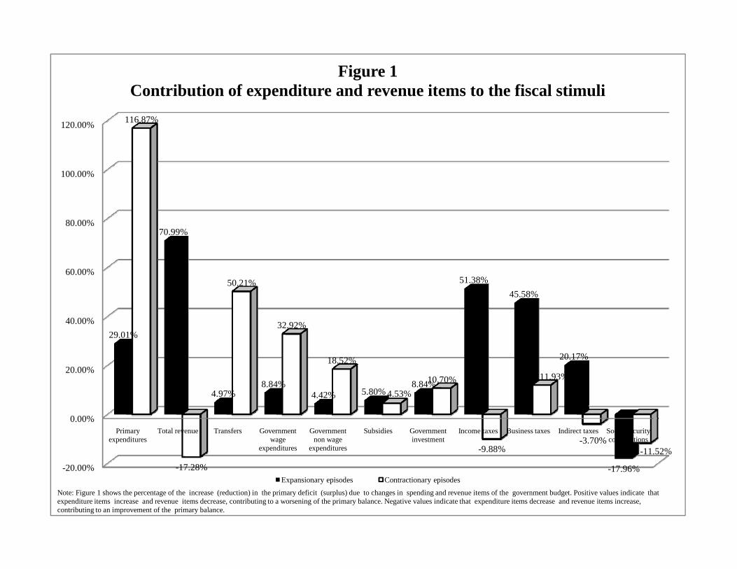
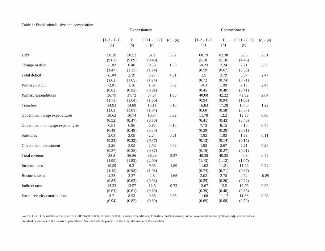
Let’s begin by analyzing what happens with fiscal stimuli, namely whether we candetect differences in the effects of fiscal packages depending on their compositionon the economy. Table 1 shows the composition in terms of spending componentsand revenue components of the 20 years of expansionary fiscal stimulus packagesversus the others. In Tables 1-6, the period [T − 2, T − 1] is the two year periodpreceding the first year of a fiscal stimulus/adjustment. The period [T ] is the firstyear and the period [T + 1, T + 2] is the two year period following the beginningof an episode.8 All the variables in the tables are yearly averages.

The most striking result of this table is that in expansionary episodes totalspending increases by roughly 1 per cent of GDP while revenues fall by morethan 2.5 per cent of GDP. In contractionary episodes total spending goes up by

7More details on these sensitivity analysis are available from the authors.8The Denmark fiscal contraction is the only episode lasting 4 years. We have included the values

of the variables in 1986 in the column [T + 1, T + 2]. We checked and confirm that the qualitativenature of the results does not change if the period [T ] inlcudes all the years of a tight/expansionaryepisode of fiscal policy and the period [T + 1, T + 2] is the two year period following the last yearof an episode.

10

close to 3 per cent of GDP while revenues are roughly constant in terms of GDP.This correlation seems to suggest that stimulus packages used upon the spendingside do not work or at least not as well as those based upon spending increases.In terms of components of spending we note that there is no difference betweenexpansionary and contractionary episodes regarding public investment which goesup by roughly the same amount in ratios of GDP. All the other components ofprimary spending and, in particular transfers, go up much more in contractionaryepisodes. This suggests that the non public investment components of the bud-get are those which explain the different correlation with growth. As for revenuesnote the large cut in income taxes in expansionary stimuli and the slight increasein contractionary ones. Not surprisingly the debt over GDP ratio goes up less inexpansionary episodes since the denominator increases more.

Figure 1 offers a striking visual image of the different compositions in termsof revenues and spending of expansionary and contractionary episodes. The firsttwo comparison of total spending and revenues are rather striking even visually.In Table 2 we look at the different components of GDP to check whether thereare difference in composition between expansionary and contractionary episodes.The first two lines which refer to GDP growth are somewhat obvious since theyreflect the selection criteria of these episodes. All the components of aggregatedemand grow more after the stimulus in expansionary episodes. This result is abit different than that reported in Alesina and Ardagna (1998). In that sample thedifference between the two types of episodes seemed concentrated on investmentrather than consumption.9 In this sample both consumption and investment behavedifferently, both increasing in expansionary cases and declining in contractionaryones. This table also allows us to check whether the state of the economy beforethe adjustments was different in the two groups. In terms of domestic growth andrelative to G7 average, expansionary episodes occurred when growth was higher.As for the other components the only significant difference seem to be in the tradebalance. It is obviously cavalier to draw broad conclusions from this but enormousdifferences in the preexisting state of the economy do not jump out from this table.

3.2 Fiscal adjustments

Fiscal adjustments can be judged in two ways, as discussed above. One is aboutwhether they have been successful in significantly reducing deficits and the debtover GDP ratios and second whether they have been associated with a reductionin growth or not. Obviously, the two criteria are correlated since a growth en-hancing adjustment is more likely to be successful in reducing the debt-to-GDP

9See Also Alesina, Ardagna Perotti and Schiantarelli (2002) for related work on the effect offiscal policy on investment.

11

ratio. However, the correlation is not perfect since a fiscal adjustment may lead toa sharp reduction of the debt/GDP ratio because the numerator drops faster thanthe denominator. Episodes with this characteristic, that is the ability to reduce thedebt-to-GDP ratio exist, for example Netherlands in 1993, Norway in 1989, andSweden in 1986-1987.

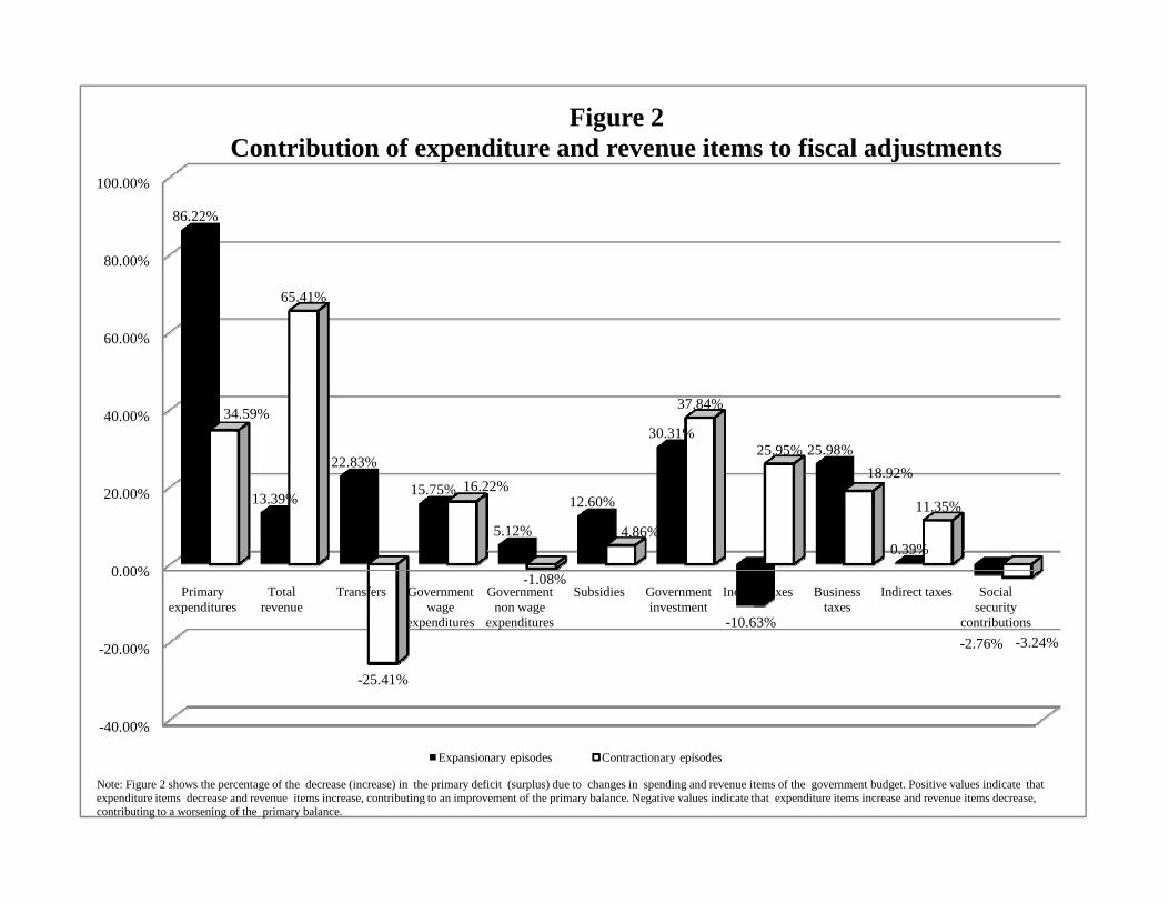
Table 3 is organized in the same way as Table 1 above. The expansionaryepisodes of fiscal adjustments are mostly characterized by spending cuts. Primaryspending as a percent of GDP falls by more than 2 per cent. Total revenues in-stead increase slightly by about 0.34 per cent of GDP. On the other hand, in thecase of contractionary fiscal adjustments primary spending is cut by about 0.7 percent of GDP, while revenues increase by about 1.2 per cent of GDP. Thus, fiscaladjustments occurring on the spending side have superior effects on growth thanthose based upon increases in tax revenues. As far as the composition in compo-nents probably the most striking difference between the two types of adjustmentshas to do with the role of transfers. In contractionary cases transfers continue togrowth as a percentage of GDP of almost half of a percentage point. In expansion-ary episodes, instead, transfers fall by roughly the same amount. Thus, in betweenthe two types of episodes there is a very large difference of 1 per cent of GDP in theshare of transfers. Looking at the composition of revenues one is struck by incometaxes: they go down quite significantly in expansionary adjustments and go up incontractionary ones. The difference between the two is almost 1 percentage pointof GDP. This difference is by far the largest among revenue components.

Figure 2 is organized in the same way as figure 1 and even in this case visuallythe contrast between the two types of fiscal adjustments is quite obvious. Whenwe look at the different components of GDP, we find that both consumption andinvestment grow more during expansionary episodes. We did not uncover any re-markable composition effects, along the same line a Table 2 displayed for fiscalstimuli. These sample statistics are reported in Table 4 which is organized as Ta-ble 2. The other interesting observation is that at least in terms of GDP growthand growth of its components the preexisting conditions of expansionary and con-tractionary episodes look remarkably similar. One rather remarkable observationcomes from comparing the growth performance during expansionary stimuli andexpansionary adjustments: they are quite similar!

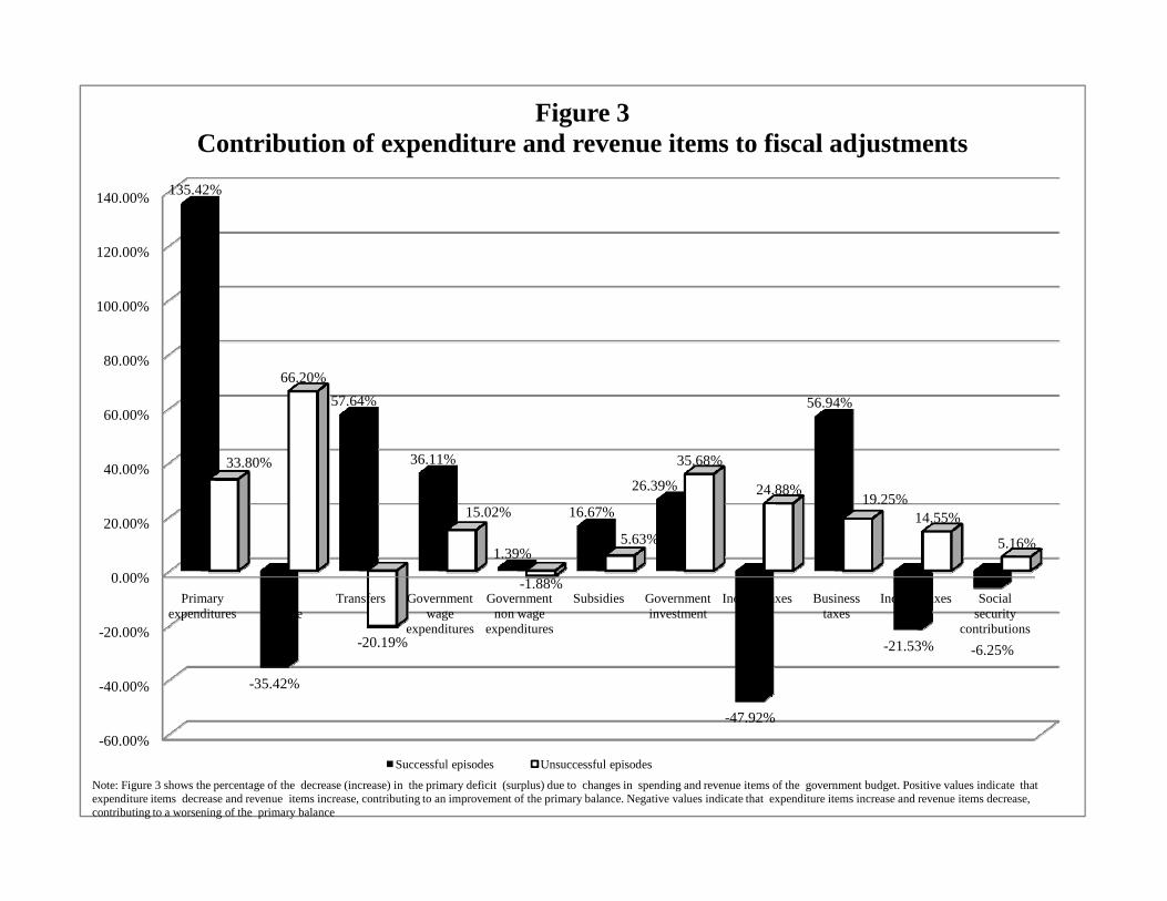
Let’s now consider successful versus unsuccessful adjustments as shown inTable 5. The comparison between the two is especially striking. In successfulepisodes total primary spending as a percentage of GDP falls by about 2 per centof GDP. Total revenues actually decline of about half of percentage point of GDP.Thus, successful fiscal adjustments are completely based on spending cuts accom-panied by modest tax cuts! On the contrary, in unsuccessful adjustments totalrevenue goes up by almost 1.5 per cent of GDP and primary spending are cut by

12

about 0.8 of GDP. Once again this comparison points in the direction of spendingcuts as the more successful ways of fixing budget problems.

Regarding the composition of spending and revenue the most striking com-parison is given by the transfers item. In successful adjustments transfers fall by0.83 per cent of GDP, while in unsuccessful adjustments they grow at about 0.4per cent, a huge difference between the two episodes of 1.2 percent of GDP. Thiscomparison points in a clear direction: it is very difficult if not impossible to fixpublic finances when in trouble without solving the question of automatic increasesin entitlements. Regarding the composition of revenues, again as above the moststriking difference is on income taxes. Figure 3, once again, gives a striking visualimage of these results.

4 Some regressions

In this section we present some simple regressions on GDP growth as a functionof changes of fiscal policy in the recent past. We should put up-front the fact thatcausality issues are all over the place here and we do not claim to have solved them.These regressions should be viewed as correlations, but we find them instructiveand the message which they send is on the same line of that emerging from ourdescriptive analysis above.

Let’s begin with fiscal stimuli. In Table 7, columns 1-4, we regress real GDPgrowth in a year of fiscal stimulus on its one period and two period lagged values,on the lagged value of the weighted average of the real GDP growth of the G7countries, on the lagged value of the ratio of public debt to GDP ratio and on aset of fiscal policy variables measuring the size and the composition of the fiscalstimulus. Columns 5-8 are analogous to the previous 4 columns except for the lhsvariable, now equal to the average of real GDP growth in a year of fiscal stimulusand in the two following ones.

We find that, controlling for initial conditions, a one percentage point higherincrease in the current spending to GDP ratio is associated with a 0.75 percentagepoint lower growth. The effect is statistically significant at the 5% level. Instead,larger increases in spending on capital goods or larger cuts in taxes do not have sta-tistically significant effects on growth (see column 2). When we try to investigatewhether the size of the fiscal stimulus or its composition is relevant for economicgrowth, we find more evidence in favor of the composition. We measure the size ofthe fiscal stimulus with the change in the cyclically adjusted primary balance. Wemeasure the composition of fiscal stimuli with two different variables: (i) the ratiobetween the change in current spending to GDP ratio and the change in the primarybalance (columns 3 and 7), and (ii) the sum of the change in current spending and

13

tax revenue to GDP ratios (column 4 and 8) to account for the fact that both currentspending increases and tax increases can be negatively associated with growth.Both measures of composition are statistically significant at the 5% level in allspecifications. In column 3, the sign of the ratio between the change in currentspending to GDP ratio and the change in the primary balance indicates that thelarger the share of the worsening in the primary balance due to spending increasesthe lower GDP growth. On average, during years of fiscal stimuli about 54% ofthe deterioration in the primary balance is due to increases in current spendingitems. A one standard deviation increase in this variable (equal to 51%, undoubt-edly a very large number) would reduce growth by 1 percentage point. Finally, alarger increase in the primary deficit to GDP ratio is associated with lower growth,however, the effect is statistically significant only in column 3.

Table 8 is very similar to Table 7 but we replace the change in current spend-ing and taxes with their respective components. Consistent with the evidence inTable 7, our regressions show that fiscal stimuli more heavily based on increases incurrent spending items (government wage and non-wage components, subsidies)are associated with lower growth, while fiscal stimulus packages based on cuts inincome, business and indirect taxes are more likely to be expansionary.

When we turn to the sample of fiscal adjustments (Tables 9 and 10), our resultsstill point in the same direction: namely, the composition of the fiscal adjustment,more than its size, matters for growth and fiscal adjustments associated with higherGDP growth are those in which a larger share of the reduction of the primarydeficit-to-GDP ratio is due to cuts in current spending, to the government wageand non-wage components, and to subsidies. All this evidence is consistent withthe previous literature on fiscal stabilizations and is robust if we introduce amongthe regressors the change in the short-term interest rate as a control for the stanceof monetary policy or the rate of change of the nominal exchange rate to controlfor exchange rate devaluations that can occur at the same time of large changes inthe fiscal stance (results are not shown but are available upon request).

Finally, we have estimated the same specifications as in Tables 7 and 9, columns1, 2, and 4 for the entire sample of OECD data that, hence, includes episodes offiscal adjustments, stimuli and years in which the cyclically adjusted primary bal-ance changes between -1.5% and 1.5%. We have also checked whether there arenon-linearities associated with times of large fiscal adjustments and stimuli. Table11 shows the results.10 Results are in line with the evidence shown so far: wefind that larger reductions in current spending and in taxation are associated withhigher GDP growth, while changes in capital spending do not show any significanteffect on growth. Moreover, the specifications in columns 4-9, do not support any

10Regressions in Table 11 include country and year dummies among the rhs variables.

14

evidence of non-linearities in episodes of fiscal adjustments or stimuli. Both thecoefficients of the dummy variables T ight and Loose and the coefficients betweenthe interaction terms of these variables and the fiscal policy indicators are not sta-tistically significant. As suggested by Alesina, Ardagna, Perotti, and Schiantarelli(2002), there seems to be nothing special around such episodes that can explain thebehavior of growth relatively to normal times.

5 Conclusions

Rather than reviewing again our result it is worth elaborating, or perhaps speculat-ing on the current and future fiscal stance in the US. As we well know a very largeportion of the current astronomical 12 percent of GDP deficit is the result of bailoutof various types of the financial sector. This is an issue on which this paper hasnothing to say. But part of the deficit is the result of the stimulus package that waspassed to lift the economy out of the recession. About two third of this fiscal pack-age is constituted by increases in spending, including public investment, transfersand government consumption. According to our results fiscal stimuli based upontax cut are much more likely to be growth enhancing than those on the spendingside. Needless to say when considering a single episode many other factors jumpto mind, factors which are difficult to capture in a multi country regressions. Forinstance, American families were saving too little before the crisis. An incometax cut might have just simply been saved and might have had not a big impact onaggregate consumption. However, more saving might have reinforced the finan-cial sector, think of the credit card crisis for instance. In addition, one could havethough of tax cuts that stimulate investment. The benefit of infrastructure projectswhich have "long and variable lags" is much more questionable.

After the "perfect storm" of this current crisis the US will emerge with anunprecedented (for peace time) increase in government debt. As we argued in theintroduction it is unlikely that these deficits and debt will disappear simply becausegrowth will resume at very rapid pace very soon. Primary suppresses would beneeded since interest rates cannot go other than up from the close to zero actuallevels. The analysis of the present paper suggests that unless primary spending iscut, it is difficult to acheive fiscal stability because spending may rise faster thantax revenue. But what can be cut? Hopefully improvements in the peace process inAfghanistan and Iraq might allow a reduction of military expenditure, but given theinstability in the region one cannot count on that for sure. Health care reforms seemto imply large increases in spending, the retirement of the baby boomers is not toofar, and in the pressing time of the crisis the issue of Social Security has been inthe background, but it has not disappeared A relatively high unemployment for a

15

couple of more years will require spending on subsidies. The budget outlook looksrather grim on the spending side. The Congressional Budget Office predicts deficitof 7 per cent of GDP up to 2020. This is not a rosy scenario.

References

[1] Aghion Philippe, Alberto Alesina and Francesco Trebbi (2004) "EndogenousPolitical Institutions" Quarterly Journal of Economics, 119, 565-612

[2] Alesina Alberto (1988) “The End of Large Public Debts” in F. Giavazzi andL. Spaventa (eds.), High Public Debt: The Italian Experience, Cambridge,Cambridge University Press.

[3] Alesina A., and S. Ardagna, 1998, Tales of Fiscal Adjustments, EconomicPolicy, October 1998, 489-545.

[4] Alesina A., S. Ardagna, R. Perotti, and F. Schiantarelli, 2002, Fiscal Policy,Profits, and Investment, American Economic Review, vol. 92, no. 3, June2002, 571-589.

[5] Alesina, Alberto and Allan Drazen (1991) “Why are Stabilizations De-layed?,” American Economic Review, 81, 1170-1188.

[6] Alesina, Alberto and Edward Glaeser (2004) Fighting Poverty in the US andEurope: A World of Difference (Oxford University Press, Oxford, UK).

[7] Alesina A., R. Perotti, and J. Tavares, 1998, The Political Economy of FiscalAdjustments, Brookings Papers on Economic Activity, Spring 1998.

[8] Alesina A., and R. Perotti, 1997, The Welfare State and Competitiveness,American Economic Review, 1997, 87, 921-939.

[9] Alesina A., and R. Perotti, 1995, Fiscal Expansions and Adjustments inOECD Countries, Economic Policy, n.21, 207-247.

[10] Ardagna Silvia (2004), “Fiscal Stabilizations: When Do They Work andWhy”, European Economic Review, vol. 48, No. 5, October 2004, pp. 1047-1074.

[11] Blanchard O., 1993, Suggestion for a New Set of Fiscal Indicators, OECDWorking paper.

[12] Blanchard O., 1990, Comment on Giavazzi and Pagano, NBER Macroeco-nomics Annual, MIT Press, Cambridge, MA, 1990.

16

[13] Blanchard, O.J.. and R. Perotti, (2002), “An Empirical Investigation of theDynamic Effects of Changes in Government Spending and Revenues on Out-put”, Quarterly Journal of Economics, November, pp. 1329-1368.

[14] Bertola, G., Drazen, A., 1993. Trigger Points and Budget Cuts: Explainingthe effects of Fiscal Austerity. American Economic Review 83 (1), 11–26.

[15] Giavazzi, F., T. Jappelli, and M. Pagano, 2000, Searching for Non-LinearEffects of Fiscal Policy: Evidence from Industrial and Developing Countries,European Economic Review, 2000, vol. 44, n.7, 1259-1289.

[16] Giavazzi F., and M. Pagano, 1996, Non-Keynesian Effects of Fiscal PolicyChanges: International Evidence and the Swedish Experience, Swedish Eco-nomic Policy Review, vol. 3, n.1, Spring, 67-112.

[17] Giavazzi F., and M. Pagano, 1990, Can Severe Fiscal Contractions Be Expan-sionary? Tales of Two Small European Countries, NBER MacroeconomicsAnnual, MIT Press, (Cambridge, MA), 1990, 95-122.

[18] Lambertini L., and J. Tavares, 2001, Exchange Rates and Fiscal Adjustments:Evidence from the ECD and Implications for EMU.

[19] McDermott J., and R. Wescott, 1996, An Empirical Analysis of Fiscal Ad-justments, IMF Staff papers, vol. 43, n.4, 723-753.

[20] Milesi-Ferretti Gian Maria, Roberto Perotti, and Massimo Rostagno (2002)“Electoral Systems And Public Spending”, The Quarterly Journal of Eco-nomics, vol. 117(2), 609-657.

[21] Mountford A., H. Uhlig, (2008), “What Are the Effects of Fiscal PlicyShocks?” NBER working paper 14551.

[22] Perotti, Roberto, 1999, Fiscal Policy When Things are Going Badly, Quar-terly Journal of Economics, 114, November 1999, 1399-1436.

[23] Persson Torsten and Guido Tabellini, (2003), “The Economic Effects of Con-stitutions”, MIT Press, Munich Lectures in Economics.

[24] Ramey V., (2008), “Identifying Government Spending Shocks: It’s All in theTiming”

[25] Romer Christina and David Romer, (2007), The Macroeconomics Effects ofTax Change: Estimates Based on a New Measure of Fiscal Shocks”, NBERworking paper 13264.

17

[26] Sutherland, A., 1997. Fiscal Crises and Aggregate Demand: Can High PublicDebt Reverse the Effects of Fiscal Policy? Journal of Public Economics 65,147–162.

[27] von Hagen J., A. H. Hallett, R. Strauch, (2002), “Budgetary Consolidationin Europe: Quality, Economic Conditions, and Persistence”, Journal of theJapanese and International Economics, vol. 16, pp. 512-535.

[28] von Hagen J., R. Strauch, (2001), “Fiscal Consolidations: Quality, EconomicConditions, and Success, Public Choice, vol. 109, no.3-4, pp 327-346

18

6 Data Appendix

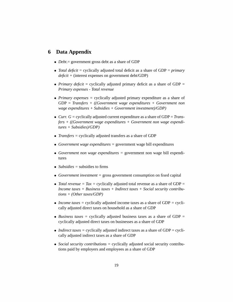
• Debt.= government gross debt as a share of GDP

• Total deficit = cyclically adjusted total deficit as a share of GDP = primarydeficit + (interest expenses on government debt/GDP)

• Primary deficit = cyclically adjusted primary deficit as a share of GDP =Primary expenses - Total revenue

• Primary expenses = cyclically adjusted primary expenditure as a share ofGDP = Transfers + ((Government wage expenditures + Government nonwage expenditures + Subsidies + Government investment)/GDP)

• Curr. G = cyclically adjusted current expenditure as a share of GDP = Trans-fers + ((Government wage expenditures + Government non wage expendi-tures + Subsidies)/GDP)

• Transfers = cyclically adjusted transfers as a share of GDP

• Government wage expenditures = government wage bill expenditures

• Government non wage expenditures = government non wage bill expendi-tures

• Subsidies = subsidies to firms

• Government investment = gross government consumption on fixed capital

• Total revenue = Tax = cyclically adjusted total revenue as a share of GDP =Income taxes + Business taxes + Indirect taxes + Social security contribu-tions + (Other taxes/GDP)

• Income taxes = cyclically adjusted income taxes as a share of GDP = cycli-cally adjusted direct taxes on household as a share of GDP

• Business taxes = cyclically adjusted business taxes as a share of GDP =cyclically adjusted direct taxes on businesses as a share of GDP

• Indirect taxes = cyclically adjusted indirect taxes as a share of GDP = cycli-cally adjusted indirect taxes as a share of GDP

• Social security contributions = cyclically adjusted social security contribu-tions paid by employers and employees as a share of GDP

19

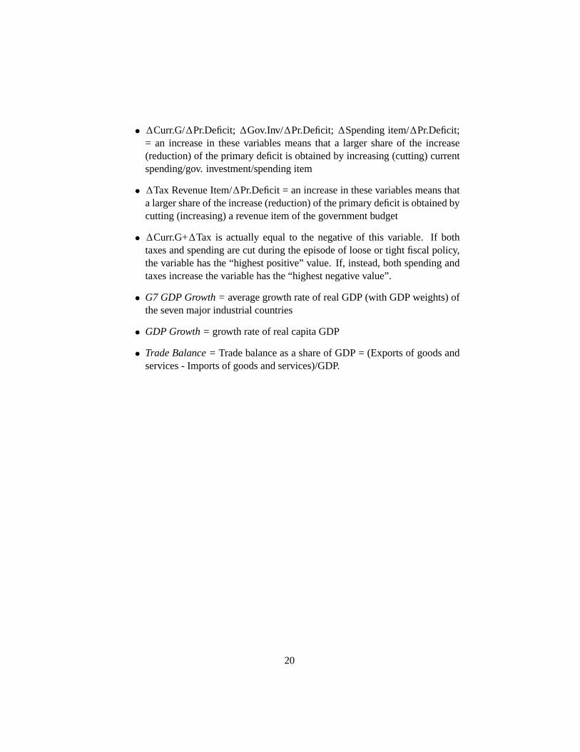
• Curr.G/ Pr.Deficit; Gov.Inv/ Pr.Deficit; Spending item/ Pr.Deficit;= an increase in these variables means that a larger share of the increase(reduction) of the primary deficit is obtained by increasing (cutting) currentspending/gov. investment/spending item

• Tax Revenue Item/ Pr.Deficit = an increase in these variables means thata larger share of the increase (reduction) of the primary deficit is obtained bycutting (increasing) a revenue item of the government budget

• Curr.G+ Tax is actually equal to the negative of this variable. If bothtaxes and spending are cut during the episode of loose or tight fiscal policy,the variable has the “highest positive” value. If, instead, both spending andtaxes increase the variable has the “highest negative value”.

• G7 GDP Growth = average growth rate of real GDP (with GDP weights) ofthe seven major industrial countries

• GDP Growth = growth rate of real capita GDP

• Trade Balance = Trade balance as a share of GDP = (Exports of goods andservices - Imports of goods and services)/GDP.

20

60.00%

80.00%

100.00%

120.00%

70.99%

51.38%45.58%

116.87%

50.21%

Figure 1Contribution of expenditure and revenue items to the fiscal stimuli

-20.00%

0.00%

20.00%

40.00%

Primary expenditures

Total revenue Transfers Government wage

expenditures

Government non wage

expenditures

Subsidies Government investment

Income taxes Business taxes Indirect taxes Social security contributions

29.01%

4.97%8.84%

4.42% 5.80%8.84%

20.17%

-17.96%-17.28%

32.92%

18.52%

4.53%10.70%

-9.88%

11.93%

-3.70%-11.52%

Expansionary episodes Contractionary episodesNote: Figure 1 shows the percentage of the increase (reduction) in the primary deficit (surplus) due to changes in spending and revenue items of the government budget. Positive values indicate that expenditure items increase and revenue items decrease, contributing to a worsening of the primary balance. Negative values indicate that expenditure items decrease and revenue items increase, contributing to an improvement of the primary balance.

20.00%

40.00%

60.00%

80.00%

100.00%

86.22%

13 39%

22.83%

15.75%12 60%

30.31%25.98%

34.59%

65.41%

16.22%

37.84%

25.95%18.92%

11 35%

Figure 2Contribution of expenditure and revenue items to fiscal adjustments

-40.00%

-20.00%

0.00%Primary

expendituresTotal

revenueTransfers Government

wage expenditures

Government non wage

expenditures

Subsidies Government investment

Income taxes Business taxes

Indirect taxes Social security

contributions

13.39%

5.12%

12.60%

-10.63%

0.39%

-2.76%

-25.41%

-1.08%

4.86%

11.35%

-3.24%

Expansionary episodes Contractionary episodes

Note: Figure 2 shows the percentage of the decrease (increase) in the primary deficit (surplus) due to changes in spending and revenue items of the government budget. Positive values indicate that expenditure items decrease and revenue items increase, contributing to an improvement of the primary balance. Negative values indicate that expenditure items increase and revenue items decrease, contributing to a worsening of the primary balance.

40.00%

60.00%

80.00%

100.00%

120.00%

140.00% 135.42%

57.64%

36.11%

26.39%

56.94%

33.80%

66.20%

35.68%

24.88% 19 25%

Figure 3Contribution of expenditure and revenue items to fiscal adjustments

-60.00%

-40.00%

-20.00%

0.00%

20.00%

Primary expenditures

Total revenue

Transfers Government wage

expenditures

Government non wage

expenditures

Subsidies Government investment

Income taxes Business taxes

Indirect taxes Social security

contributions

-35.42%

1.39%

16.67%

-47.92%

-21.53% -6.25%-20.19%

15.02%

-1.88%

5.63%

19.25%14.55%

5.16%

Successful episodes Unsuccessful episodes

Note: Figure 3 shows the percentage of the decrease (increase) in the primary deficit (surplus) due to changes in spending and revenue items of the government budget. Positive values indicate that expenditure items decrease and revenue items increase, contributing to an improvement of the primary balance. Negative values indicate that expenditure items increase and revenue items decrease, contributing to a worsening of the primary balance

(0 33) (0 32) (0 37) (0 13) (0 14) (0 15)

Table 1: Fiscal stimuli: size and compositionExpansionary Contractionary

[T-2 - T-1] T [T+1 - T+2] (c) - (a) [T-2 - T-1] T [T+1 - T+2] (c) - (a)(a) (b) (c) (a) (b) (c)

Debt 50.28 50.52 51.1 0.82 60.79 62.38 63.3 2.51(9.03) (9.09) (9.48) (5.18) (5.18) (4.46)

Change in debt -1.02 0.48 0.53 1.55 -0.29 2.24 2.21 2.50(1.47) (1.12) (1.24) (0.59) (0.67) (0.68)

Total deficit -1.04 2.19 3.27 4.31 1.5 3.79 3.97 2.47(1.62) (1.65) (1.24) (0.72) (0.74) (0.71)

Primary deficit -2.01 1.16 1.61 3.62 -0.3 1.99 2.13 2.43(0.82) (0.92) (0.91) (0.45) (0.48) (0.41)

Primary expenditures 36.79 37.72 37.84 1.05 40.08 42.22 42.92 2.84(1.73) (1.64) (1.66) (0.94) (0.94) (1.00)

Transfers 14.93 14.88 15.11 0.18 16.83 17.28 18.05 1.22(1.03) (1.01) (1.04) (0.60) (0.58) (0.57)

Government wage expenditures 10.62 10.74 10.94 0.32 11.78 12.2 12.58 0.80(0.52) (0.47) (0.50) (0.41) (0.43) (0.46)

Government non wage expenditures 6.81 6.96 6.97 0.16 7.73 8.15 8.18 0.45(0.49) (0.49) (0.55) (0.29) (0.28) (0.31)

Subsidies 2.03 2.09 2.24 0.21 1.82 1.93 1.93 0.11(0.33) (0 32). .(0 37) (0 13). (0 14) (0 15). .

Government investment 2.26 3.05 2.58 0.32 1.95 2.67 2.21 0.26(0.37) (0.38) (0.37) (0.19) (0.27) (0.21)

Total revenue 38.8 36.56 36.23 -2.57 40.38 40.23 40.8 0.42(1.90) (1.83) (2.00) (1.15) (1.12) (1.07)

Income taxes 10.89 9.2 9.03 -1.86 11.02 11.21 11.26 0.24(1.10) (0.98) (1.08) (0.74) (0.71) (0.67)

Business taxes 4.25 3.37 2.6 -1.65 3.03 2.78 2.74 -0.29(0.83) (0.63) (0.33) (0.25) (0.20) (0.22)

Indirect taxes 13.33 12.57 12.6 -0.73 12.67 12.5 12.76 0.09(0.61) (0.61) (0.69) (0.39) (0.40) (0.36)

Social security contributions 8.7 8.93 9.35 0.65 11.08 11.17 11.36 0.28(0.94) (0.82) (0.89) (0.69) (0.68) (0.70)

Source: OECD. Variables are in share of GDP. Total deficit, Primary deficit, Primary expenditures, Transfers, Total revenues, and all revenue items are cyclically adjusted variables. Standard deviations of the means in parenthesis. See the Data Appendix for the exact definition of the variables

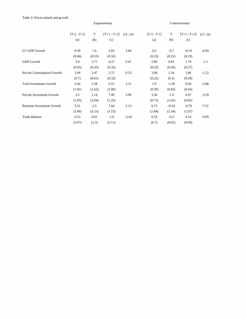
Table 2: Fiscal stimuli and growth

[T-2 - T-1] T [T+1 - T+2] (c) - (a) [T-2 - T-1] T [T+1 - T+2] (c) - (a)

(a) (b) (c) (a) (b) (c)

G7 GDP Growth 0.39 1.6 2.03 1.64 0.2 -0.7 -0.74 -0.94

(0.66) (0.53) (0.32) (0.23) (0.23) (0.19)

GDP Growth 3.9 3.77 4.37 0.47 2.89 0.93 1.79 -1.1

(0.65) (0.35) (0.32) (0.22) (0.26) (0.27)

Private Consumption Growth 3.49 3.47 3.72 0.23 3.08 1.54 1.86 -1.22

(0.7) (0.61) (0.32) (0.22) (0.3) (0.29)

Total Investment Growth 3.44 2.58 6.55 3.11 2.9 -1.39 0.04 -2.86

(1.81) (1.63) (1.00) (0.59) (0.82) (0.64)

Private Investment Growth 3.5 1.14 7.49 3.99 3.36 -1.9 0.07 -3.29

(2.05) (2.04) (1.25) (0.73) (1.02) (0.82)

Business Investment Growth 5.51 2.5 7.64 2.13 6.73 -0.34 -0.78 -7.51

(2.06) (3.21) (1.53) (1.44) (1.34) (1.07)

Trade Balance 0.53 0.61 -1.9 -2.43 0.19 -0.2 0.14 -0.05

(2.07) (2.2) (2.11) (0.7) (0.65) (0.69)

Expansionary Contractionary

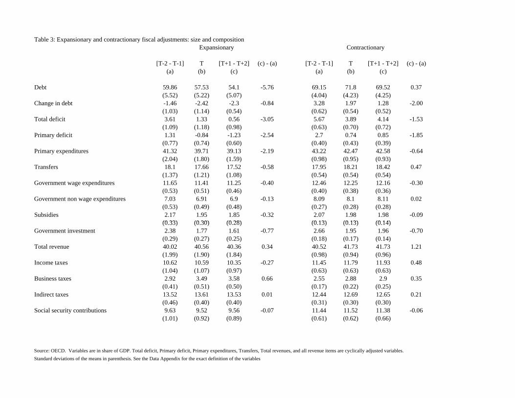
(0 33) (0 30) (0 28) (0 13) (0 13) (0 14)

Table 3: Expansionary and contractionary fiscal adjustments: size and compositionExpansionary Contractionary

[T-2 - T-1] T [T+1 - T+2] (c) - (a) [T-2 - T-1] T [T+1 - T+2] (c) - (a)(a) (b) (c) (a) (b) (c)

Debt 59.86 57.53 54.1 -5.76 69.15 71.8 69.52 0.37(5.52) (5.22) (5.07) (4.04) (4.23) (4.25)

Change in debt -1.46 -2.42 -2.3 -0.84 3.28 1.97 1.28 -2.00(1.03) (1.14) (0.54) (0.62) (0.54) (0.52)

Total deficit 3.61 1.33 0.56 -3.05 5.67 3.89 4.14 -1.53(1.09) (1.18) (0.98) (0.63) (0.70) (0.72)

Primary deficit 1.31 -0.84 -1.23 -2.54 2.7 0.74 0.85 -1.85(0.77) (0.74) (0.60) (0.40) (0.43) (0.39)

Primary expenditures 41.32 39.71 39.13 -2.19 43.22 42.47 42.58 -0.64(2.04) (1.80) (1.59) (0.98) (0.95) (0.93)

Transfers 18.1 17.66 17.52 -0.58 17.95 18.21 18.42 0.47(1.37) (1.21) (1.08) (0.54) (0.54) (0.54)

Government wage expenditures 11.65 11.41 11.25 -0.40 12.46 12.25 12.16 -0.30(0.53) (0.51) (0.46) (0.40) (0.38) (0.36)

Government non wage expenditures 7.03 6.91 6.9 -0.13 8.09 8.1 8.11 0.02(0.53) (0.49) (0.48) (0.27) (0.28) (0.28)

Subsidies 2.17 1.95 1.85 -0.32 2.07 1.98 1.98 -0.09(0.33) .(0 30) .(0 28) (0 13). (0 13) (0 14). .

Government investment 2.38 1.77 1.61 -0.77 2.66 1.95 1.96 -0.70(0.29) (0.27) (0.25) (0.18) (0.17) (0.14)

Total revenue 40.02 40.56 40.36 0.34 40.52 41.73 41.73 1.21(1.99) (1.90) (1.84) (0.98) (0.94) (0.96)

Income taxes 10.62 10.59 10.35 -0.27 11.45 11.79 11.93 0.48(1.04) (1.07) (0.97) (0.63) (0.63) (0.63)

Business taxes 2.92 3.49 3.58 0.66 2.55 2.88 2.9 0.35(0.41) (0.51) (0.50) (0.17) (0.22) (0.25)

Indirect taxes 13.52 13.61 13.53 0.01 12.44 12.69 12.65 0.21(0.46) (0.40) (0.40) (0.31) (0.30) (0.30)

Social security contributions 9.63 9.52 9.56 -0.07 11.44 11.52 11.38 -0.06(1.01) (0.92) (0.89) (0.61) (0.62) (0.66)

Source: OECD. Variables are in share of GDP. Total deficit, Primary deficit, Primary expenditures, Transfers, Total revenues, and all revenue items are cyclically adjusted variables. Standard deviations of the means in parenthesis. See the Data Appendix for the exact definition of the variables

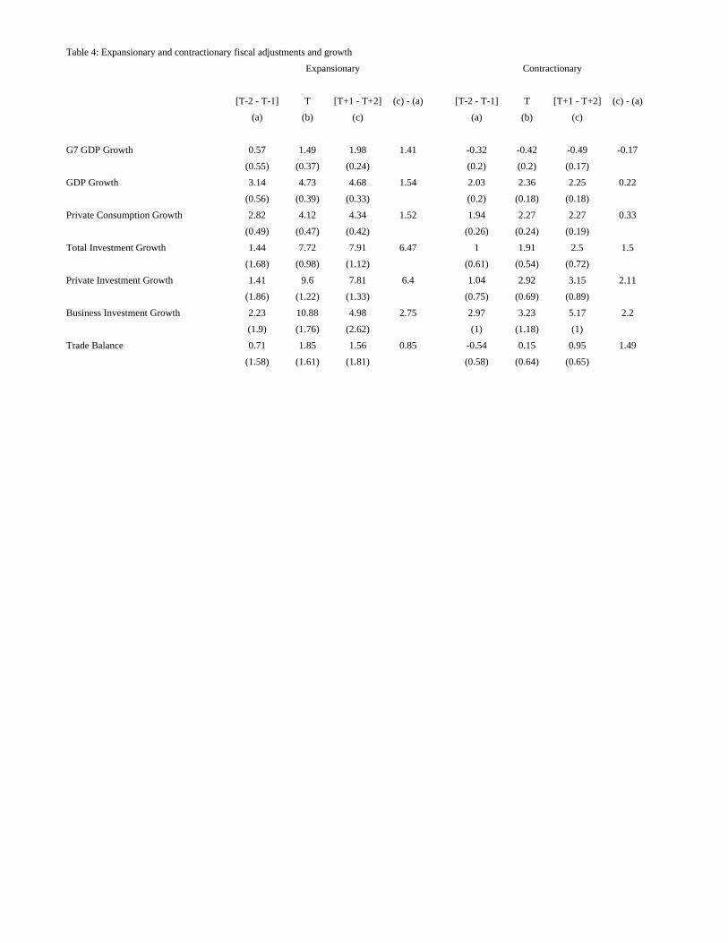
Table 4: Expansionary and contractionary fiscal adjustments and growth

[T-2 - T-1] T [T+1 - T+2] (c) - (a) [T-2 - T-1] T [T+1 - T+2] (c) - (a)

(a) (b) (c) (a) (b) (c)

G7 GDP Growth 0.57 1.49 1.98 1.41 -0.32 -0.42 -0.49 -0.17

(0.55) (0.37) (0.24) (0.2) (0.2) (0.17)

GDP Growth 3.14 4.73 4.68 1.54 2.03 2.36 2.25 0.22

(0.56) (0.39) (0.33) (0.2) (0.18) (0.18)

Private Consumption Growth 2.82 4.12 4.34 1.52 1.94 2.27 2.27 0.33

(0.49) (0.47) (0.42) (0.26) (0.24) (0.19)

Total Investment Growth 1.44 7.72 7.91 6.47 1 1.91 2.5 1.5

(1.68) (0.98) (1.12) (0.61) (0.54) (0.72)

Private Investment Growth 1.41 9.6 7.81 6.4 1.04 2.92 3.15 2.11

(1.86) (1.22) (1.33) (0.75) (0.69) (0.89)

Business Investment Growth 2.23 10.88 4.98 2.75 2.97 3.23 5.17 2.2

(1.9) (1.76) (2.62) (1) (1.18) (1)

Trade Balance 0.71 1.85 1.56 0.85 -0.54 0.15 0.95 1.49

(1.58) (1.61) (1.81) (0.58) (0.64) (0.65)

Expansionary Contractionary

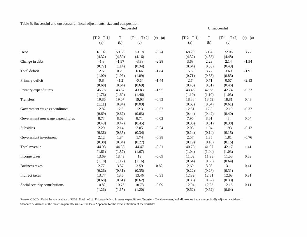
(0 36) (0 35) (0 34) (0 14) (0 14) (0 15)

Table 5: Successful and unsuccessful fiscal adjustments: size and compositionSuccessful Unsuccessful

[T-2 - T-1] T [T+1 - T+2] (c) - (a) [T-2 - T-1] T [T+1 - T+2] (c) - (a)(a) (b) (c) (a) (b) (c)

Debt 61.92 59.63 53.18 -8.74 68.29 71.4 72.06 3.77(4.32) (4.50) (4.16) (4.32) (4.53) (4.48)

Change in debt -1.6 -1.97 -3.88 -2.28 3.68 2.29 2.14 -1.54(0.72) (1.14) (0.34) (0.64) (0.53) (0.43)

Total deficit 2.5 0.29 0.66 -1.84 5.6 3.77 3.69 -1.91(1.00) (1.06) (1.09) (0.71) (0.83) (0.85)

Primary deficit 0.8 -1.2 -0.64 -1.44 2.7 0.71 0.57 -2.13(0.68) (0.64) (0.69) (0.45) (0.51) (0.46)

Primary expenditures 45.78 43.67 43.83 -1.95 43.46 42.68 42.74 -0.72(1.76) (1.60) (1.46) (1.10) (1.10) (1.03)

Transfers 19.86 19.07 19.03 -0.83 18.38 18.59 18.81 0.43(1.11) (0.94) (0.89) (0.63) (0.64) (0.61)

Government wage expenditures 12.82 12.5 12.3 -0.52 12.51 12.3 12.19 -0.32(0.69) (0.67) (0.63) (0.44) (0.42) (0.40)

Government non wage expenditures 8.73 8.62 8.71 -0.02 7.96 8.01 8 0.04(0.49) (0.47) (0.45) (0.30) (0.31) (0.30)

Subsidies 2.29 2.14 2.05 -0.24 2.05 1.94 1.93 -0.12(0.36) .(0 35) .(0 34) (0 14). (0 14) (0 15). .

Government investment 2.12 1.34 1.74 -0.38 2.57 1.85 1.81 -0.76(0.38) (0.34) (0.27) (0.19) (0.18) (0.16)

Total revenue 44.98 44.86 44.47 -0.51 40.76 41.97 42.17 1.41(1.61) (1.57) (1.67) (1.04) (1.04) (1.03)

Income taxes 13.69 13.43 13 -0.69 11.02 11.35 11.55 0.53(1.18) (1.17) (1.16) (0.64) (0.65) (0.64)

Business taxes 2.77 3.37 3.59 0.82 2.69 3.08 3.1 0.41(0.26) (0.31) (0.35) (0.22) (0.28) (0.31)

Indirect taxes 13.77 13.6 13.46 -0.31 12.32 12.51 12.63 0.31(0.68) (0.61) (0.62) (0.33) (0.32) (0.33)

Social security contributions 10.82 10.73 10.73 -0.09 12.04 12.25 12.15 0.11(1.26) (1.15) (1.20) (0.62) (0.62) (0.64)

Source: OECD. Variables are in share of GDP. Total deficit, Primary deficit, Primary expenditures, Transfers, Total revenues, and all revenue items are cyclically adjusted variables. Standard deviations of the means in parenthesis. See the Data Appendix for the exact definition of the variables

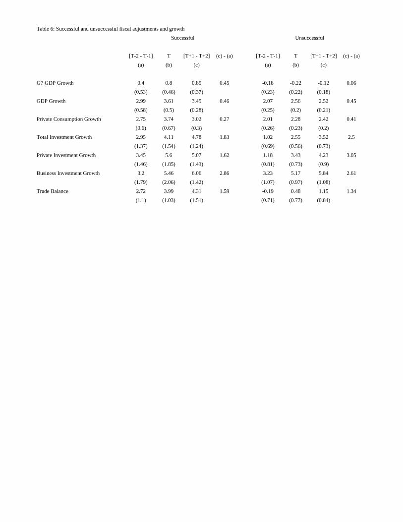
Table 6: Successful and unsuccessful fiscal adjustments and growth

[T-2 - T-1] T [T+1 - T+2] (c) - (a) [T-2 - T-1] T [T+1 - T+2] (c) - (a)

(a) (b) (c) (a) (b) (c)

G7 GDP Growth 0.4 0.8 0.85 0.45 -0.18 -0.22 -0.12 0.06

(0.53) (0.46) (0.37) (0.23) (0.22) (0.18)

GDP Growth 2.99 3.61 3.45 0.46 2.07 2.56 2.52 0.45

(0.58) (0.5) (0.28) (0.25) (0.2) (0.21)

Private Consumption Growth 2.75 3.74 3.02 0.27 2.01 2.28 2.42 0.41

(0.6) (0.67) (0.3) (0.26) (0.23) (0.2)

Total Investment Growth 2.95 4.11 4.78 1.83 1.02 2.55 3.52 2.5

(1.37) (1.54) (1.24) (0.69) (0.56) (0.73)

Private Investment Growth 3.45 5.6 5.07 1.62 1.18 3.43 4.23 3.05

(1.46) (1.85) (1.43) (0.81) (0.73) (0.9)

Business Investment Growth 3.2 5.46 6.06 2.86 3.23 5.17 5.84 2.61

(1.79) (2.06) (1.42) (1.07) (0.97) (1.08)

Trade Balance 2.72 3.99 4.31 1.59 -0.19 0.48 1.15 1.34

(1.1) (1.03) (1.51) (0.71) (0.77) (0.84)

Successful Unsuccessful

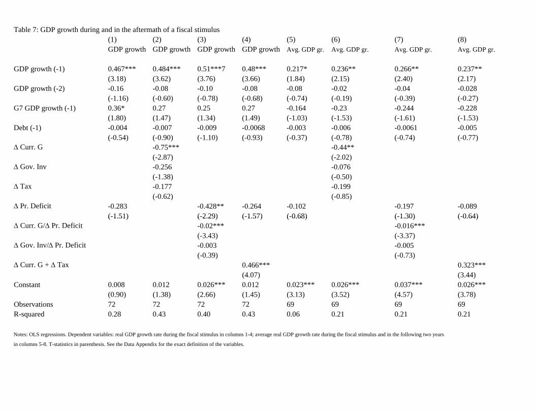
51) 29) 57) 68) 30) 64)

Table 7: GDP growth during and in the aftermath of a fiscal stimulus(1) (2) (3) (4) (5) (6) (7) (8)GDP growth GDP growth GDP growth GDP growth Avg. GDP gr. Avg. GDP gr. Avg. GDP gr. Avg. GDP gr.

GDP growth (-1) 0.467*** 0.484*** 0.51***7 0.48*** 0.217* 0.236** 0.266** 0.237**(3.18) (3.62) (3.76) (3.66) (1.84) (2.15) (2.40) (2.17)

GDP growth (-2) -0.16 -0.08 -0.10 -0.08 -0.08 -0.02 -0.04 -0.028(-1.16) (-0.60) (-0.78) (-0.68) (-0.74) (-0.19) (-0.39) (-0.27)

G7 GDP growth (-1) 0.36* 0.27 0.25 0.27 -0.164 -0.23 -0.244 -0.228(1.80) (1.47) (1.34) (1.49) (-1.03) (-1.53) (-1.61) (-1.53)

Debt (-1) -0.004 -0.007 -0.009 -0.0068 -0.003 -0.006 -0.0061 -0.005(-0.54) (-0.90) (-1.10) (-0.93) (-0.37) (-0.78) (-0.74) (-0.77)

Δ Curr. G -0.75*** -0.44**(-2.87) (-2.02)

Δ Gov. Inv -0.256 -0.076(-1.38) (-0.50)

Δ Tax -0.177 -0.199(-0.62) (-0.85)

Δ Pr. Deficit -0.283 -0.428** -0.264 -0.102 -0.197 -0.089(-1.51)(-1. (-2.29)(-2. (-1.57) (-0.68)(-1. (-0. (-1.30) (-0.64)(-1. (-0.

Δ Curr. G/Δ Pr. Deficit -0.02*** -0.016***(-3.43) (-3.37)

Δ Gov. Inv/Δ Pr. Deficit -0.003 -0.005(-0.39) (-0.73)

Δ Curr. G + Δ Tax 0.466*** 0.323***(4.07) (3.44)

Constant 0.008 0.012 0.026*** 0.012 0.023*** 0.026*** 0.037*** 0.026***(0.90) (1.38) (2.66) (1.45) (3.13) (3.52) (4.57) (3.78)

Observations 72 72 72 72 69 69 69 69R-squared 0.28 0.43 0.40 0.43 0.06 0.21 0.21 0.21

Notes: OLS regressions. Dependent variables: real GDP growth rate during the fiscal stimulus in columns 1-4; average real GDP growth rate during the fiscal stimulus and in the following two years

in columns 5-8. T-statistics in parenthesis. See the Data Appendix for the exact definition of the variables.

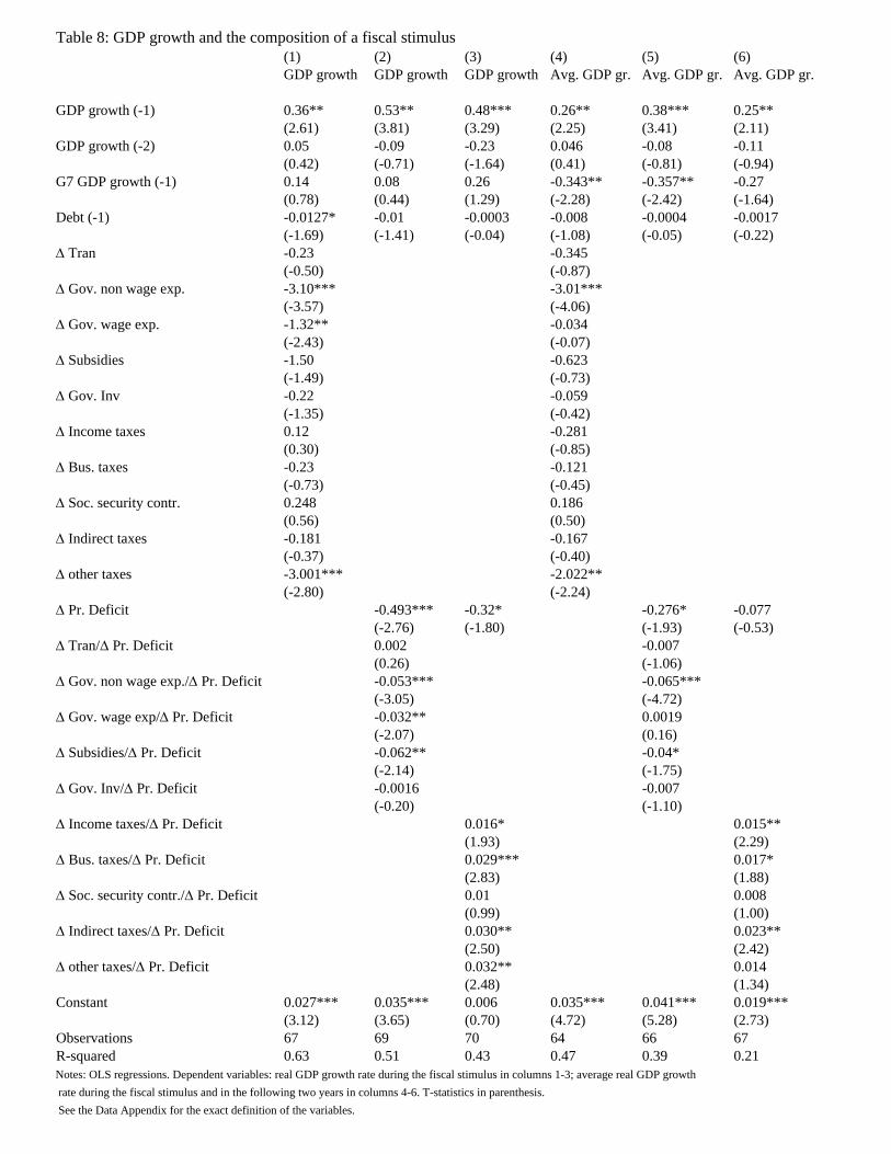
Table 8: GDP growth and the composition of a fiscal stimulus(1) (2) (3) (4) (5) (6)GDP growth GDP growth GDP growth Avg. GDP gr. Avg. GDP gr. Avg. GDP gr.

GDP growth (-1) 0.36** 0.53** 0.48*** 0.26** 0.38*** 0.25**(2.61) (3.81) (3.29) (2.25) (3.41) (2.11)

GDP growth (-2) 0.05 -0.09 -0.23 0.046 -0.08 -0.11(0.42) (-0.71) (-1.64) (0.41) (-0.81) (-0.94)

G7 GDP growth (-1) 0.14 0.08 0.26 -0.343** -0.357** -0.27(0.78) (0.44) (1.29) (-2.28) (-2.42) (-1.64)

Debt (-1) -0.0127* -0.01 -0.0003 -0.008 -0.0004 -0.0017(-1.69) (-1.41) (-0.04) (-1.08) (-0.05) (-0.22)

Δ Tran -0.23 -0.345(-0.50) (-0.87)

Δ Gov. non wage exp. -3.10*** -3.01***(-3.57) (-4.06)

Δ Gov. wage exp. -1.32** -0.034(-2.43) (-0.07)

Δ Subsidies -1.50 -0.623(-1.49) (-0.73)

Δ Gov. Inv -0.22 -0.059(-1.35) (-0.42)

Δ Income taxes 0.12 -0.281(0.30) (-0.85)

Δ Bus. taxes -0.23 -0.121(-0.73) (-0.45)

Δ Soc. security contr. 0.248 0.186(0.56) (0.50)

Δ Indirect taxes -0.181 -0.167(-0.37)( ) (-0.40)( )

Δ other taxes -3.001*** -2.022**(-2.80) (-2.24)

Δ Pr. Deficit -0.493*** -0.32* -0.276* -0.077(-2.76) (-1.80) (-1.93) (-0.53)

Δ Tran/Δ Pr. Deficit 0.002 -0.007(0.26) (-1.06)

Δ Gov. non wage exp./Δ Pr. Deficit -0.053*** -0.065***(-3.05) (-4.72)

Δ Gov. wage exp/Δ Pr. Deficit -0.032** 0.0019(-2.07) (0.16)

Δ Subsidies/Δ Pr. Deficit -0.062** -0.04*(-2.14) (-1.75)

Δ Gov. Inv/Δ Pr. Deficit -0.0016 -0.007(-0.20) (-1.10)

Δ Income taxes/Δ Pr. Deficit 0.016* 0.015**(1.93) (2.29)

Δ Bus. taxes/Δ Pr. Deficit 0.029*** 0.017*(2.83) (1.88)

Δ Soc. security contr./Δ Pr. Deficit 0.01 0.008(0.99) (1.00)

Δ Indirect taxes/Δ Pr. Deficit 0.030** 0.023**(2.50) (2.42)

Δ other taxes/Δ Pr. Deficit 0.032** 0.014(2.48) (1.34)

Constant 0.027*** 0.035*** 0.006 0.035*** 0.041*** 0.019***(3.12) (3.65) (0.70) (4.72) (5.28) (2.73)

Observations 67 69 70 64 66 67R-squared 0.63 0.51 0.43 0.47 0.39 0.21Notes: OLS regressions. Dependent variables: real GDP growth rate during the fiscal stimulus in columns 1-3; average real GDP growth rate during the fiscal stimulus and in the following two years in columns 4-6. T-statistics in parenthesis.S h A di f h d fi i i f h i bl See the Data Appendix for the exact definition of the variables.

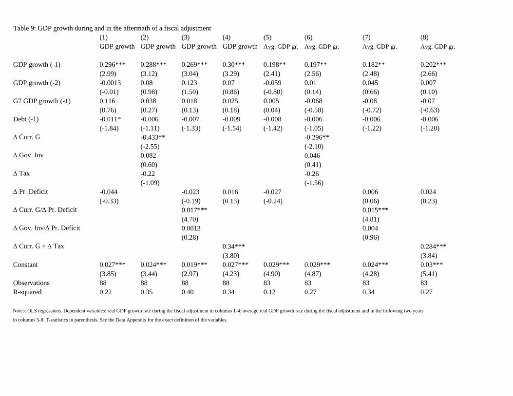
Δ G/Δ fi 0 017*** 0 015***

Table 9: GDP growth during and in the aftermath of a fiscal adjustment(1) (2) (3) (4) (5) (6) (7) (8)GDP growth GDP growth GDP growth GDP growth Avg. GDP gr. Avg. GDP gr. Avg. GDP gr. Avg. GDP gr.

GDP growth (-1) 0.296*** 0.288*** 0.269*** 0.30*** 0.198** 0.197** 0.182** 0.202***(2.99) (3.12) (3.04) (3.29) (2.41) (2.56) (2.48) (2.66)

GDP growth (-2) -0.0013 0.08 0.123 0.07 -0.059 0.01 0.045 0.007(-0.01) (0.98) (1.50) (0.86) (-0.80) (0.14) (0.66) (0.10)

G7 GDP growth (-1) 0.116 0.038 0.018 0.025 0.005 -0.068 -0.08 -0.07(0.76) (0.27) (0.13) (0.18) (0.04) (-0.58) (-0.72) (-0.63)

Debt (-1) -0.011* -0.006 -0.007 -0.009 -0.008 -0.006 -0.006 -0.006(-1.84) (-1.11) (-1.33) (-1.54) (-1.42) (-1.05) (-1.22) (-1.20)

Δ Curr. G -0.433** -0.296**(-2.55) (-2.10)

Δ Gov. Inv 0.082 0.046(0.60) (0.41)

Δ Tax -0.22 -0.26(-1.09) (-1.56)

Δ Pr. Deficit -0.044 -0.023 0.016 -0.027 0.006 0.024(-0.33) (-0.19) (0.13) (-0.24) (0.06) (0.23)

Δ Curr G/Δ Pr Deficit Curr. Pr. De cit 0 017***. 0 015***.(4.70) (4.81)

Δ Gov. Inv/Δ Pr. Deficit 0.0013 0.004(0.28) (0.96)

Δ Curr. G + Δ Tax 0.34*** 0.284***(3.80) (3.84)

Constant 0.027*** 0.024*** 0.019*** 0.027*** 0.029*** 0.029*** 0.024*** 0.03***(3.85) (3.44) (2.97) (4.23) (4.90) (4.87) (4.28) (5.41)

Observations 88 88 88 88 83 83 83 83R-squared 0.22 0.35 0.40 0.34 0.12 0.27 0.34 0.27

Notes: OLS regressions. Dependent variables: real GDP growth rate during the fiscal adjustment in columns 1-4; average real GDP growth rate during the fiscal adjustment and in the following two years

in columns 5-8. T-statistics in parenthesis. See the Data Appendix for the exact definition of the variables.

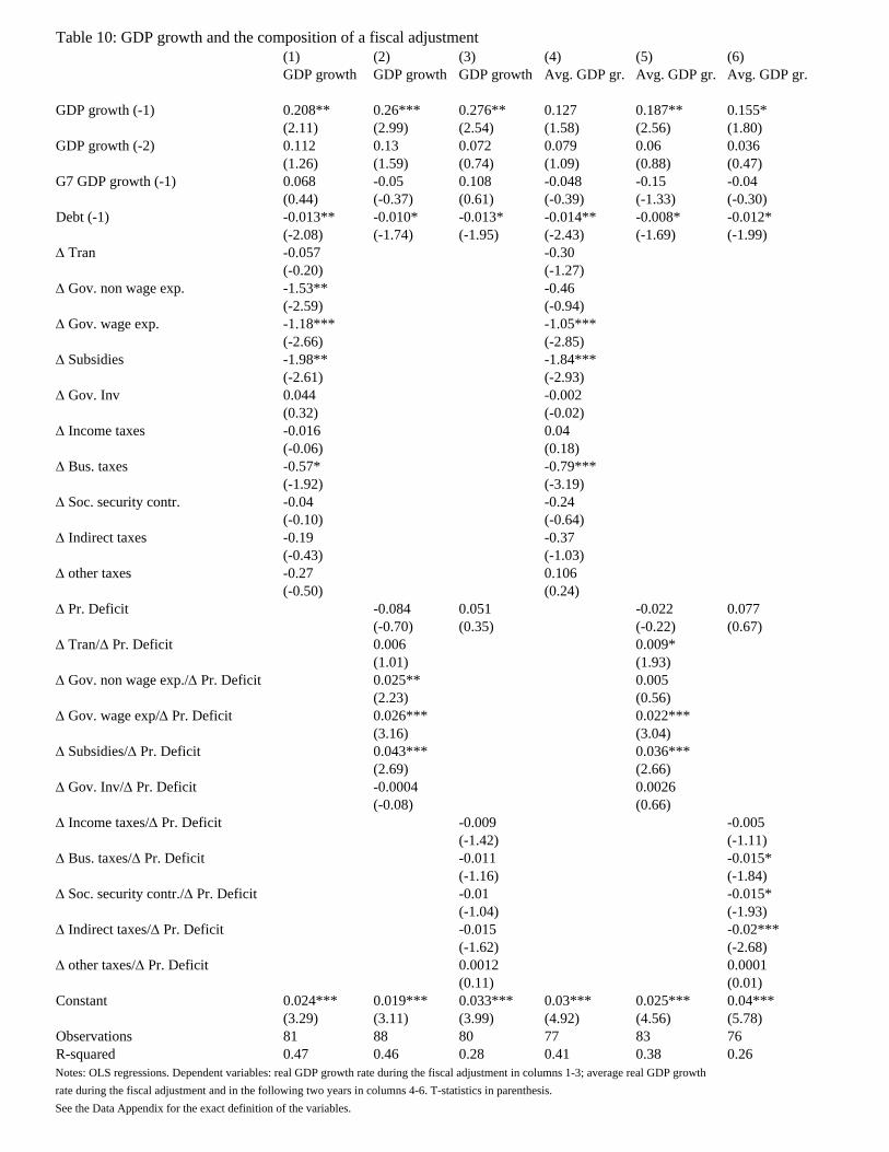
Table 10: GDP growth and the composition of a fiscal adjustment(1) (2) (3) (4) (5) (6)GDP growth GDP growth GDP growth Avg. GDP gr. Avg. GDP gr. Avg. GDP gr.

GDP growth (-1) 0.208** 0.26*** 0.276** 0.127 0.187** 0.155*(2.11) (2.99) (2.54) (1.58) (2.56) (1.80)

GDP growth (-2) 0.112 0.13 0.072 0.079 0.06 0.036(1.26) (1.59) (0.74) (1.09) (0.88) (0.47)

G7 GDP growth (-1) 0.068 -0.05 0.108 -0.048 -0.15 -0.04(0.44) (-0.37) (0.61) (-0.39) (-1.33) (-0.30)

Debt (-1) -0.013** -0.010* -0.013* -0.014** -0.008* -0.012*(-2.08) (-1.74) (-1.95) (-2.43) (-1.69) (-1.99)

Δ Tran -0.057 -0.30(-0.20) (-1.27)

Δ Gov. non wage exp. -1.53** -0.46(-2.59) (-0.94)

Δ Gov. wage exp. -1.18*** -1.05***(-2.66) (-2.85)

Δ Subsidies -1.98** -1.84***(-2.61) (-2.93)

Δ Gov. Inv 0.044 -0.002(0.32) (-0.02)

Δ Income taxes -0.016 0.04(-0.06) (0.18)

Δ Bus. taxes -0.57* -0.79***(-1.92) (-3.19)

Δ Soc. security contr. -0.04 -0.24(-0.10) (-0.64)

Δ Indirect taxes -0.19 -0.37(-0.43)( ) (-1.03)( )

Δ other taxes -0.27 0.106(-0.50) (0.24)

Δ Pr. Deficit -0.084 0.051 -0.022 0.077(-0.70) (0.35) (-0.22) (0.67)

Δ Tran/Δ Pr. Deficit 0.006 0.009*(1.01) (1.93)

Δ Gov. non wage exp./Δ Pr. Deficit 0.025** 0.005(2.23) (0.56)

Δ Gov. wage exp/Δ Pr. Deficit 0.026*** 0.022***(3.16) (3.04)

Δ Subsidies/Δ Pr. Deficit 0.043*** 0.036***(2.69) (2.66)

Δ Gov. Inv/Δ Pr. Deficit -0.0004 0.0026(-0.08) (0.66)

Δ Income taxes/Δ Pr. Deficit -0.009 -0.005(-1.42) (-1.11)

Δ Bus. taxes/Δ Pr. Deficit -0.011 -0.015*(-1.16) (-1.84)

Δ Soc. security contr./Δ Pr. Deficit -0.01 -0.015*(-1.04) (-1.93)

Δ Indirect taxes/Δ Pr. Deficit -0.015 -0.02***(-1.62) (-2.68)

Δ other taxes/Δ Pr. Deficit 0.0012 0.0001(0.11) (0.01)

Constant 0.024*** 0.019*** 0.033*** 0.03*** 0.025*** 0.04***(3.29) (3.11) (3.99) (4.92) (4.56) (5.78)

Observations 81 88 80 77 83 76R-squared 0.47 0.46 0.28 0.41 0.38 0.26Notes: OLS regressions. Dependent variables: real GDP growth rate during the fiscal adjustment in columns 1-3; average real GDP growth rate during the fiscal adjustment and in the following two years in columns 4-6. T-statistics in parenthesis. S h A di f h d fi i i f h i blSee the Data Appendix for the exact definition of the variables.

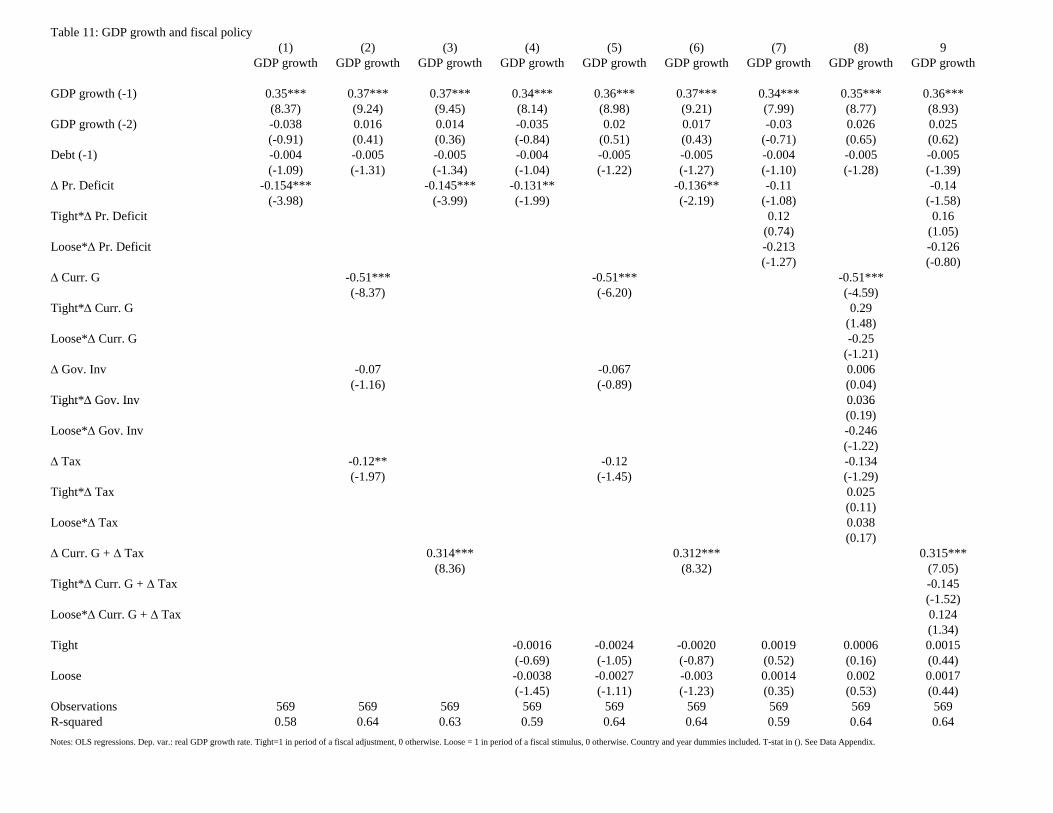
Δ Inv 0.036

Table 11: GDP growth and fiscal policy(1) (2) (3) (4) (5) (6) (7) (8) 9

GDP growth GDP growth GDP growth GDP growth GDP growth GDP growth GDP growth GDP growth GDP growth

GDP growth (-1) 0.35*** 0.37*** 0.37*** 0.34*** 0.36*** 0.37*** 0.34*** 0.35*** 0.36***(8.37) (9.24) (9.45) (8.14) (8.98) (9.21) (7.99) (8.77) (8.93)

GDP growth (-2) -0.038 0.016 0.014 -0.035 0.02 0.017 -0.03 0.026 0.025(-0.91) (0.41) (0.36) (-0.84) (0.51) (0.43) (-0.71) (0.65) (0.62)

Debt (-1) -0.004 -0.005 -0.005 -0.004 -0.005 -0.005 -0.004 -0.005 -0.005(-1.09) (-1.31) (-1.34) (-1.04) (-1.22) (-1.27) (-1.10) (-1.28) (-1.39)

Δ Pr. Deficit -0.154*** -0.145*** -0.131** -0.136** -0.11 -0.14(-3.98) (-3.99) (-1.99) (-2.19) (-1.08) (-1.58)

Tight*Δ Pr. Deficit 0.12 0.16(0.74) (1.05)

Loose*Δ Pr. Deficit -0.213 -0.126(-1.27) (-0.80)

Δ Curr. G -0.51*** -0.51*** -0.51***(-8.37) (-6.20) (-4.59)

Tight*Δ Curr. G 0.29(1.48)

Loose*Δ Curr. G -0.25(-1.21)

Δ Gov. Inv -0.07 -0.067 0.006(-1.16) (-0.89) (0.04)

Tight*Δ Gov. InvTight Gov. 0.036(0.19)

Loose*Δ Gov. Inv -0.246(-1.22)

Δ Tax -0.12** -0.12 -0.134(-1.97) (-1.45) (-1.29)

Tight*Δ Tax 0.025(0.11)

Loose*Δ Tax 0.038(0.17)

Δ Curr. G + Δ Tax 0.314*** 0.312*** 0.315***(8.36) (8.32) (7.05)

Tight*Δ Curr. G + Δ Tax -0.145(-1.52)

Loose*Δ Curr. G + Δ Tax 0.124(1.34)

Tight -0.0016 -0.0024 -0.0020 0.0019 0.0006 0.0015(-0.69) (-1.05) (-0.87) (0.52) (0.16) (0.44)

Loose -0.0038 -0.0027 -0.003 0.0014 0.002 0.0017(-1.45) (-1.11) (-1.23) (0.35) (0.53) (0.44)

Observations 569 569 569 569 569 569 569 569 569R-squared 0.58 0.64 0.63 0.59 0.64 0.64 0.59 0.64 0.64Notes: OLS regressions. Dep. var.: real GDP growth rate. Tight=1 in period of a fiscal adjustment, 0 otherwise. Loose = 1 in period of a fiscal stimulus, 0 otherwise. Country and year dummies included. T-stat in (). See Data Appendix.

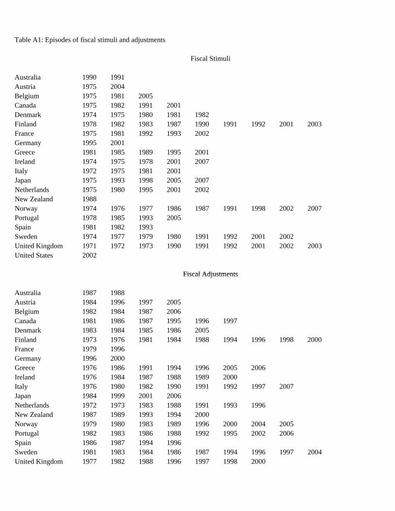
Fisca Adj men s

Table A1: Episodes of fiscal stimuli and adjustments

Fiscal Stimuli

Australia 1990 1991Austria 1975 2004Belgium 1975 1981 2005Canada 1975 1982 1991 2001Denmark 1974 1975 1980 1981 1982Finland 1978 1982 1983 1987 1990 1991 1992 2001 2003France 1975 1981 1992 1993 2002Germany 1995 2001Greece 1981 1985 1989 1995 2001Ireland 1974 1975 1978 2001 2007Italy 1972 1975 1981 2001Japan 1975 1993 1998 2005 2007Netherlands 1975 1980 1995 2001 2002New Zealand 1988Norway 1974 1976 1977 1986 1987 1991 1998 2002 2007Portugal 1978 1985 1993 2005Spain 1981 1982 1993Sweden 1974 1977 1979 1980 1991 1992 2001 2002United Kingdom 1971 1972 1973 1990 1991 1992 2001 2002 2003United States 2002

Fiscal Adjustmentsl ust t

Australia 1987 1988Austria 1984 1996 1997 2005Belgium 1982 1984 1987 2006Canada 1981 1986 1987 1995 1996 1997Denmark 1983 1984 1985 1986 2005Finland 1973 1976 1981 1984 1988 1994 1996 1998 2000France 1979 1996Germany 1996 2000Greece 1976 1986 1991 1994 1996 2005 2006Ireland 1976 1984 1987 1988 1989 2000Italy 1976 1980 1982 1990 1991 1992 1997 2007Japan 1984 1999 2001 2006Netherlands 1972 1973 1983 1988 1991 1993 1996New Zealand 1987 1989 1993 1994 2000Norway 1979 1980 1983 1989 1996 2000 2004 2005Portugal 1982 1983 1986 1988 1992 1995 2002 2006Spain 1986 1987 1994 1996Sweden 1981 1983 1984 1986 1987 1994 1996 1997 2004United Kingdom 1977 1982 1988 1996 1997 1998 2000

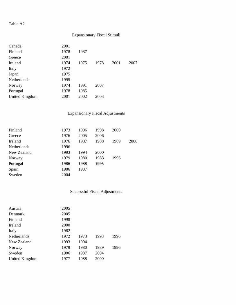
uga 1986 1988 1995

Table A2

Expansionary Fiscal Stimuli

Canada 2001Finland 1978 1987Greece 2001Ireland 1974 1975 1978 2001 2007Italy 1972Japan 1975Netherlands 1995Norway 1974 1991 2007Portugal 1978 1985United Kingdom 2001 2002 2003

Expansionary Fiscal Adjustments

Finland 1973 1996 1998 2000Greece 1976 2005 2006Ireland 1976 1987 1988 1989 2000Netherlands 1996New Zealand 1993 1994 2000Norway 1979 1980 1983 1996PortugalPort l 1986 1988 1995Spain 1986 1987Sweden 2004

Successful Fiscal Adjustments

Austria 2005Denmark 2005Finland 1998Ireland 2000Italy 1982Netherlands 1972 1973 1993 1996New Zealand 1993 1994Norway 1979 1980 1989 1996Sweden 1986 1987 2004United Kingdom 1977 1988 2000