Risk-based Loan Pricing: Portfolio Optimization

Approach With Marginal Risk Contribution

So Yeon ChunMcDonough School of Business, Georgetown University, Washington D.C. 20057, soyeon.chun@georgetown.edu

Miguel A. LejeuneDepartment of Decision Sciences, George Washington University, Washington, DC 20052, mlejeune@gwu.edu

We consider a lender (bank) who determines the optimal loan price (interest rates) to offer to prospective

borrowers under uncertain risk and borrower response. A borrower may or may not accept the loan at the

price offered, and in the presence of default risk, both the principal loaned and the interest income become

uncertain. We present a risk-based loan pricing optimization model, which explicitly takes into account

marginal risk contribution, portfolio risk, and borrower’s acceptance probability. Marginal risk assesses the

amount a prospective loan would contribute to the bank’s loan portfolio risk by capturing the interrelation-

ship between a prospective loan and the existing loans in the portfolio and is evaluated with respect to the

Value-at-Risk and Conditional-Value-at-Risk risk measures. We examine the properties and computational

difficulties of the associated formulations. Then, we design a concavifiability reformulation method that

transforms the nonlinear objective function of the loan pricing problems and permits to derive equivalent

mixed-integer nonlinear reformulations with convex continuous relaxations. We discuss managerial implica-

tions of the proposed model and test the computational tractability of the proposed solution approach.

Key words : risk-based pricing, revenue management, loan portfolio, marginal risk contribution,

Value-at-Risk, Conditional Value-at-Risk, willingness-to-pay, mixed-integer nonlinear stochastic

programming

1. Introduction

Lending is the primary business activity for most commercial banks. The loan portfolio is usually

the largest asset and the predominant source of revenue but also carries a significant exposure

to credit risk (Mercer 1992, Stanhouse and Stock 2008). Although specific loan agreement terms

and conditions vary, one of the most critical elements controlling the performance and risk of the

loan portfolio is the interest rate, which can be referred to as the price of a loan. Importance

and challenges of the structured loan pricing have been recognized by many practitioners (e.g.,

PwC 2012, BCG 2016, Sageworks 2016). For example, BCG points out that advanced pricing

techniques embraced by an ever-expanding variety of businesses have not been yet adopted in

commercial lending, causing forgone revenue of 7% to 10%. Sageworks also recognizes that banks

could significantly increase the revenue if they had more structured pricing methodologies in place.

1

2

PWC mentions “As companies realize the inefficiency and unreliability of the traditional loan

pricing strategies, we believe a trend toward a pricing optimization” in loan pricing.

Until the early 1990s, banks simply posted one price (“house rate”) for each loan type and

rejected most high-risk borrowers (Johnson 1992). Following the financial reforms1, improvement

of the underwriting technologies, and drop in data storage cost in recent years, however, banks

started to manage their risks more effectively by adopting so called risk-based pricing : estimate

the specific risk of each borrower and offer different prices (interest rates) to different borrowers

and transactions (Bostic 2002, Thomas 2009).

The rationale behind risk-based pricing is rather straightforward. A lender should charge higher

prices for borrowers with higher default risk and larger potential losses since they are more costly.

Notably, the key element to such a pricing strategy is to identify the risks that are being priced.

In a typical loan underwriting process, banks make approval and pricing decisions based on an

estimate of the borrower’s probability of default (PD), which is usually assessed by the credit

rating/scores (e.g., Moody’s, S&P and Fitch ratings) and loss given default (LGD), which is the

amount of money a bank loses if a borrower defaults (see, e.g., Gupton et al. 2002, Phillips 2013

for more details). While recognizing the risk posed by each loan is essential for the optimal loan

pricing, there are some limitations and challenges in the current application of this pricing strategy.

It should be first noted that the performance of the entire loan portfolio does not only depend

on the risk of individual loans, but also on the interrelationships between the loans in the portfolio.

In fact, the concept of portfolio management is not new in finance and optimization models have

been widely used in the financial industry to build optimal portfolios of securities and to manage

market risk (see, e.g., Cornuejols and Tutuncu 2007, DeMiguel et al. 2009, Kawas and Thiele 2011,

Dentcheva and Ruszczynski 2015, and references therein). However, the use of such optimization

models remains limited in credit risk, in particular to determine the price at which to grant the

loan (see Allen and Saunders 2002 and Kimber 2003 for general reviews on credit portfolio risk

management). In terms of loan pricing, the portfolio optimization approach suggests that instead

of relying on the “standalone risk”, the individual risk of a borrower measured in isolation, the

price of a loan should incorporate the change in the portfolio risk triggered by a new loan, or “risk

contribution”, the risk amount a prospective loan would contribute to the bank’s current loan

portfolio risk.

Evaluation of risk contributions requires the selection of risk measures in which the decomposition

of the overall portfolio credit risk into individual loan risk contributions is attainable2. To this

1 According to the database covering 91 countries over the 1973-2005 period, 74 countries in the sample had fully

liberalized lending and deposit rates by 2005, compared to four countries in 1973. Most of the countries completed

interest rate liberalization in the 1980s and 1990s (Abiad et al. 2008).

2 This view is related to a modern asset allocation and investment style called “risk budgeting” that focuses on how

risk is distributed throughout a portfolio.

Chun and Lejeune: Risk-based Loan Pricing

3

end, we consider the “marginal risk” contribution, i.e., marginal impact of a particular loan on

the overall portfolio risk, with the widely used Value-at-Risk (VaR) and Conditional-Value-at-

Risk (CVaR, also known as expected shortfall) risk measures. VaR is the risk measure initially

recommended by the internal rating-based approach preconized by the Basel Committee3 and has

been one of the most commonly used risk measures in the financial industry. On the other hand,

CVaR, which accounts for losses exceeding VaR, is now becoming the risk measure of choice for the

Basel Committee intending to “move from Value-at-Risk to Expected Shortfall” (Basel Committee

on Banking Supervision 2013). These two risk measures are positive homogeneous (the risk of a

portfolio scales proportionally to its size), and thus the marginal risk contributions with respect to

VaR and CVaR can be represented as the conditional loss expectation of a loan provided that the

losses of the entire portfolio reach a certain level (Glasserman 2006). Inclusion of such marginal

risk contributions in the pricing optimization problem poses serious computational challenges (e.g.,

non-convexity); yet it would enable the lender to directly capture the interdependence between the

prospective and existing loans in the portfolio and thus control the risk and profitability of the

loan portfolio more effectively.

Another critical element to optimal loan pricing, which is often ignored in risk-based pricing, is

the borrower’s response, the propensity of a borrower to accept the offered loan price (acceptance

probability). In many industries, such as retail and hospitality, the concepts of price response

(demand function) and willingness to pay (WTP) have been well understood. Hence, the price

optimization paradigm, which takes into account the impact of price changes on demand and profit,

has been widely adopted (e.g., Phillips 2005, Cohen et al. 2016, and references therein). Under

risk-based pricing, however, the price is still mainly based on the cost to provide a loan and to

cover potential losses; banks usually set the loan price by adding a fixed margin to total cost to

hit a target rate of return on capital (Caufield 2012, PwC 2012). While such strategy avoids the

underpricing of high risk loans, the margin (and the final price) could be too high (too low) in the

sense that lower (higher) prices maximize the total profit. This is because it overlooks variations

in the value different borrowers place on a loan (different WTP and price sensitivity), and on

bank’s specific market position and relationships with different borrowers. As a result, banks lose

opportunities to either make profitable loans (lose demand from potential borrowers with low

WTP) or make even larger profits (by offering a higher price to a borrower who is willing to pay

more). By incorporating borrowers’ acceptance probability into risk-based pricing, banks will be

3 The Basel Committee on Banking Supervision issues Basel Accords, recommendations on banking laws and regula-

tions. Basel Accords are intended to amend international standards that control how much capital banks need to hold

to guard against the financial and operational risks faced. Worldwide adoption of the Basel II Accords gave further

impetus to the use of VaR. See e.g., Basel Committee on Banking Supervision 2006 for more details.

4

able to assess the expected profits more accurately as a function of borrowers’ characteristics, price,

as well as risks. Given that banks and financial services in general have far more information on

their customers than most other industries (e.g., banks know whom they are doing business with

and whether their offers were accepted or declined at a particular price and by which customer),

they have a unique opportunity to take the price optimization practice even further.

In this paper, we consider a lender (bank) who determines the optimal loan price for prospec-

tive borrowers in order to maximize the net interest income of a loan portfolio under uncertain

response and risk. A borrower may or may not accept the loan at the price offered, and in the

presence of default risk, both the principal loaned and the interest payments become uncertain.

Our risk-based loan price optimization model explicitly takes into account two critical elements

discussed earlier: loan portfolio risk with marginal risk contribution and borrower’s response (loan

accept probability). The risk is evaluated with the VaR or CVaR measures, and we present specific

optimization formulations employing commonly used forms of demand response functions (linear,

exponential, and logit) with portfolio and marginal risk constraints. We first show that it is a non-

convex stochastic programming optimization problem, which is very difficult to solve. We examine

the properties and computational difficulties of the associated formulations. Then, we propose

a reformulation approach based on the concavifiability concept, which allows for the derivation

of equivalent mixed-integer nonlinear reformulations with continuous relaxation. We also extend

the approach to the multi-loan pricing problem, which features explicit loan selection decisions

in addition to the pricing ones. We discuss managerial implications of the proposed model and

implementations.

1.1. Relevant Literature

Loan pricing problems have received significant attention in recent years from both industry and

academia. Many practitioners recognize the importance of the structured loan pricing model in the

financial industry (e.g., PwC 2012, BCG 2016, Sageworks 2016), and some academic researchers

demonstrate that consumers’ price elasticity/WTP (e.g., Gross and Souleles 2002) and a portfolio

view (e.g., Musto and Souleles 2006) are pertinent to loan/credit pricing decision. However, most

existing studies on the loan pricing have focused on the empirical evidence of risk-based pricing

in various credit markets (e.g., Schuermann 2004, Edelberg 2006, Magri and Pico 2011). To our

knowledge, there is no quantitative loan pricing model in the literature that explicitly takes into

account both consumers’ response and interdependence between the prospective loan and the loans

in the existing portfolio. The paper attempts to fill this gap by proposing a risk-based loan pricing

optimization models incorporating both aspects and further developing efficient reformulations of

the proposed model.

Chun and Lejeune: Risk-based Loan Pricing

5

There is a sparse yet growing body of literature that incorporates the pricing angle into the

loan rate optimization problem. For example, Phillips (2013) establishes that optimizing the price

for a consumer loan involves trade-offs: increasing the price for a prospective loan reduces the

probability that the customer will accept the loan but increases profitability if the customer does

accept. He then proposes a consumer credit pricing model determining the optimal rate, which

maximizes the lender’s expected net interest income. Similarly, Oliver and Oliver (2014) emphasize

that the loan price controls not only the risk but also the profit by managing demand response, and

describe the structural solution of the loan rate as a function of default and response risk (based

on the acceptance probability of the loan given the price). Huang and Thomas (2015) use a linear

response function to model the probability that a borrower will take the loan, and study how the

Basel Accord impacts the optimal loan price, which maximizes the lender’s profit. These papers,

however, employ a standalone risk approach and do not incorporate interrelationships between

loans.

As we consider the marginal risk contribution to explicitly capture interdependence between

the prospective loan and the loans in the existing portfolio, our paper also contributes to the

literature on the portfolio management with marginal risk contribution. The concept of marginal

risk contribution has attracted increasing attention in recent years. Specifically, several researchers

have investigated the properties of marginal VaR and CVaR marginal risk contributions (see Tasche

2000, Gourieroux et al. 2000, Kurth and Tasche 2003, Merino and Nyfeler 2004, Glasserman 2006,

Liu 2015 and references therein). However, marginal risk contributions in the literature are often

discussed only in the ex post analysis context rather than as an ex ante consideration. There

are only a few very recent papers that attempt to incorporate the marginal risk concept into the

portfolio selection problem (Zhu et al. 2010, Cui et al. 2016), but these are only specific to the

mean-variance framework and overlook more computationally challenging issues associated with

downside risk metrics, such as VaR, or CVaR. As we will show later, the inclusion of both price

response function (acceptance probability) and the marginal VaR or CVaR constraint in the loan

pricing optimization model considerably increases the complexity and tractability of the problem.

Nevertheless, we propose a computationally tractable solution method that permits to concurrently

handle the ex ante estimation (prior to granting the loan) of the marginal risk and determines

the optimal interest rate. In particular, we use a concavifiability method that provides equivalent

convex reformulations of the non-convex risk pricing problems.

2. Risk-based Loan Pricing Model

We consider a lender (bank) who needs to determine the optimal prices (interest rates) to offer

to prospective borrowers to maximize the expected profit (net interest income) under uncertain

6

borrowers’ response and risk. We assume that there are n prospective loans under consideration

and n = n− n granted (existing) loans in the current loan portfolio. For each loan i = 1,2, . . . n

(prospective and existing), let xi be the price, which is written as the annual percentage rate

(APR), ai be the loan amount (principal), Li be the Loss Given Default (LGD), qi be the payment

frequency (e.g., monthly, quarterly, etc.), and Ti be the term, which is in the unit of payment

frequency4.

When a certain price is offered, the prospective borrower may or may not accept the offer. The

acceptance probability would be obviously dependent upon the price (e.g., as the price increases,

ceteris paribus, the acceptance probability would decrease). It could also depend on other charac-

teristics of the borrower (e.g., the borrower with higher risk/switching cost might be willing to pay

more. Thus, we use a price response (acceptance probability) function g(xn, sn), where xn is the

price offered and sn describes the characteristics of the borrower (e.g., credit rating, age, income

level, transaction history, etc.), to account for the likelihood of a borrower to accept the proposed

interest rate5.

Now, let us consider the case when the offer is accepted and the loan is granted. If the interest

payments are made on the agreed upon dates and the principal on the loan is paid in full at

maturity, the lender faces no default/credit risk and receives back the original principal amount

lent plus an interest income. However, if the borrower defaults, both the principal loaned and the

interest payments expected to be received are at risk, and the loss/risk magnitude depends on

the time of default. We denote by χi,t, t = 1, . . . , Ti, i = 1, . . . , n a binary random variable taking

value 0 if the borrower of loan i defaults at any time until t and taking value 1 otherwise, by

t∗i = min(∑Ti

t=1χi,t, Ti), i= 1, . . . , n the time at which the principal will be (possibly partially) repaid

(i.e., t∗i is the default time in case of default, and is otherwise the maturity of the loan i), and by

δ the (one-period) discount factor.

Then we can write down the present value of a future uncertain stream of payments (discounted

cash flow) for each loan, G(xi), i= 1, . . . , n6:

Gi(xi) =

Ti∑t=1

χi,tδtai(xi/qi) + ai(1−Li−Liχi,Ti)δ

t∗i . (1)

The first term represents the discounted value of the interest payments and the second term is the

discounted value of the repaid principal amount.

4 For instance, for a 4-year loan with a quarterly payment schedule, T = 48.

5 In Section 3.3, we discuss specific forms of the price response functions widely used in practice and provide refor-

mulations of the corresponding optimization problems.

6 Note that G(xi) also depends on χi,t, i= 1,2, . . . , n, t= 1,2, . . . , Ti. To ease the notations, we omit denoting the full

dependence.

Chun and Lejeune: Risk-based Loan Pricing

7

We next formulate the risk constraint in terms of the stochastic loss of a portfolio with respect

to the risk measure ρ(·)7. In particular, we incorporate the constraint on each loan’s marginal risk

contribution to the pre-existing portfolio, which accounts for the correlation among loans in the

portfolio. We denote the random loss of a portfolio ζ =n∑i=1

ζi where ζi = ai−Gi.

For the ease of exposition and demonstration, we first consider the case where n= 1, i.e., there

are n−1 granted loans and the lender now considers a prospective nth loan and determines xn8. Let

ρMn be the (marginal) risk contribution of a new nth loan with risk metric ρ. For risk measures with

positive homogeneity, it has been been demonstrated (see, e.g., Gourieroux et al. 2000, Kalkbrener

et al. 2004, Tasche 2009) that Euler’s theorem permits to define ρMn as:

ρMn = ρ(ζi|ζ) :=∂ρ(ζ)∂an

. (2)

That is, the risk contribution can be calculated by obtaining the first order partial derivative of a

risk measure with respect to the loan amount.9

Based on the discussion above, we can formulate the risk-based loan pricing optimization problem

with a single prospective loan, denoted as LPO as follows:

LPO : maxxn

{h(xn) := g(xn, sn)E

[(Gn(xn)− an

)]+E

[ n−1∑i=1

(Gi(xi)− ai

)]}(3)

s.t. l≤ xn ≤ u, (4)

ρMn (ζ(xn)) ≤ κMan, (5)

ρ (ζ(xn)) ≤ κP

n∑i=1

ai. (6)

The lender’s objective (3) is to maximize the expected profit taking into account uncertainties in

both demand (response) and default risk10. The constraint (4) implements possible lower and upper

bounds on the price possibly driven by the regulations (e.g., usury laws) and/or business practices

with marketing or operational considerations (e.g., price stability is desirable). The equations (5)

7 In Sections 3.1 and 3.2, we consider specific risk measures, namely VaR and CVaR and discuss reformulations in

detail.

8 This case may reflect the underwriting process of large-scale business loans (e.g., large corporate loans). In Section 4,

we extend our model and provide general formulations for the case with n > 1.

9 Different methods of calculating risk contributions have been studied for different purposes. Standalone and incre-

mental risk contribution (the change in total risk due to the inclusion of a component) are other alternatives popular

in practice. However, those violate the desirable properties for credit risk management such as diversification and

linear aggregation axioms and the sum of the incremental risk contributions across all components is generally not

equal to the risk of the entire portfolio. See, Kalkbrener (2005) and Mausser and Rosen (2008) for general discussions.

10 We could easily incorporate other costs such as funding costs (with risk-free rate), overhead/administrative

expenses, which do not depend on the price of a loan. In our formulation, those other costs are fixed and normalized

to zero.

8

and (6) represent the marginal and portfolio risk constraints with the thresholds κM and κP , which

are defined as percentages value of the potential new loan and the overall portfolio. It is implicitly

assumed that if the optimal objective value is negative, thereby indicating that it is not possible

to find an admissible interest rate giving a positive expected profit, the optimal decision is to not

extend any offer for the new loan and reject it. Later, this aspect is explicitly considered in the

multiple prospective loan case discussed in Section 4.

In the next section, we discuss the challenges in solving this optimization problem and provide

reformulations for both VaR and CVaR risk measures with several functional forms of the price-

response function.

3. Reformulations and Properties of Risk-Based Loan Pricing Model

In this section, we derive the specific VaR and CVaR formulations for the risk-pricing model LPO

presented in Section 2. First, we provide the formulation of the VaR and CVaR portfolio and

marginal risk constraints, examine their complexity, and propose a linearization approach of the

feasible set defined by the risk constraints. Next, we define several price-response functional forms,

introduce them in the formulations of the LPO models with VaR and CVaR constraints, and study

the complexity of the models. The resulting optimization problems take the form of mixed-integer

nonlinear programming (MINLP) problems (see Burer and Letchford 2012, DAmbrosio and Lodi

2011, Krokhmal et al. 2011 for reviews of the MINLP field and risk measures). For some of the

considered price-response functions, the corresponding MINLP problems are particularly complex,

since their continuous relation is not convex. Therefore, we design a concavifiability approach that

transforms the nonlinear objective function and permits to obtain convex MINLP reformulations

with identical optimal solutions (all proofs are in the Appendix).

3.1. Portfolio and Marginal VaR Constraints: Properties and Reformulations

We first consider the portfolio risk constraint (6) for the VaR measure. The Value-at-Risk qα of

the random portfolio loss ζ at the level α is defined as:

qα = inf{z : P(ζ > z)≤ α} . (7)

We decompose the portfolio loss ζ into the loss ζn due to the loan n under consideration and

the loss∑n−1

i=1 ζi due to the (n−1) loans previously granted. While the interest rate for the (n−1)

granted loans is known, the losses that might be incurred with those loans is dependent on whether

the borrowers will default or not. On the other hand, the loss ζn incurred with loan n depends on

the annual percentage rate xn that the institution has yet to determine in addition to whether the

borrower will default.

Chun and Lejeune: Risk-based Loan Pricing

9

The formulation of the portfolio risk constraint (6) for the VaR measure takes the form of a

chance constraint with random technology matrix (Kataoka 1963):

P

(an

(1−

Tn∑t=1

χn,tδtxnqn− (1−Ln +Lnχn,Tn)δt

∗n

)+

n−1∑i=1

ζi ≤ κV aRP

n∑i=1

ai

)≥ α , (8)

with P referring to a probability measure and the upper bound κV aRP

n∑i=1

ai on qα limits the autho-

rized risk. In the above formulation, the value of the threshold κV aRP

n∑i=1

ai is determined exogenously,

prior to the optimization as it is customary, and is called target (Benati and Rizzi 2007, Yu et al.

2015) or ”benchmark VaR” (Gourieroux et al. 2000)11.

We now consider the marginal risk contribution constraint (5) for the VaR measure. Specifically,

the equation (2) can be written as (Glasserman 2006):

ρMn =∂V aRα(ζ)

∂an=E[ζn|ζ = V aRα(ζ)] . (9)

The marginal VaR contribution due to loan n is equal to the expectation of the loss associated to

loan n conditional to the entire portfolio loss being equal to VaR. The magnitude of the marginal

VaR contribution is limited with the following conditional expectation constraint (Prekopa 1995):

E

[an

(1−

Tn∑t=1

χn,tδt xn

qn− (1−Ln+Lnχn,Tn )δ

t∗n

)∣∣∣∣∣an(1−

Tn∑t=1

χn,tδt xn

qn− (1−Ln+Lnχn,Tn )δ

t∗n

)+

n−1∑i=1

ζi = κP

n∑i=1

ai

]≤ κV aRM an .

(10)

If the conditional event has a positive probability to happen (Tasche 2009), the above conditional

expectation constraints is given by:

E[an

(1−

Tn∑t=1

χn,tδtxnqn

− (1−Ln+Lnχn,Tn )δt∗n

), an

(1−

Tn∑t=1

χn,tδtxnqn

− (1−Ln+Lnχn,Tn )δt∗n

)+n−1∑i=1

ζi = κPn∑i=1

ai

]P(an

(1−

Tn∑t=1

χn,tδtxnqn

− (1−Ln+Lnχn,Tn )δt∗n

)+n−1∑i=1

ζi = κPn∑i=1

ai

) ≤ κV aRM an .

(11)

Optimization problems including constraints of form (8) and (11) cannot be solved analytically,

nor by optimization solvers. We shall therefore derive equivalent reformulations of the constraints

(8) and (11) that are amenable to a numerical solution.

We proceed in two steps to derive a mixed-integer linear programming (MILP) reformulation of

the feasible set defined by the portfolio and marginal VaR constraints. The following parameter and

set notations will be used. We denote by K the scenario index set. The vector ωk = [γkn,Ok] refers

to the scenario with index k, k ∈K. Each component γkn,t of γkn ∈ {0,1}T is a Boolean indicator

taking value 0 if the prospective loan n defaults at any time until t in scenario ωk and taking value

11 An alternative would be to let the model define endogenously the value of the threshold, which would then be a

decision variable.

10

1 otherwise. Each component Oki of Ok ∈Rn−1 is the loss due to existing loan i, i= 1, . . . , n− 1 in

scenario ωk over the entire planning horizon. The probability of scenario ωk is pk with∑k∈K

pk = 1,

Mk+ and Mk− are large positive scalars, and ε is an infinitesimal positive number.

The reformulation of the feasible set will require the lifting of the decisional space and the

introduction of the following decision variables:

• zk+: non-negative variable defining the portfolio loss in excess to κV aRP

∑n

i=1 ai in scenario ωk.

• zk−: non-negative variable defining the portfolio loss below κV aRP

∑n

i=1 ai in scenario ωk.

• βk+: binary decision variable indicating whether the loss is strictly larger than κV aRP

∑n

i=1 ai

in scenario ωk (βk+ = 1) or not (βk+ = 0).

• βk−: binary decision variable indicating whether the loss is strictly smaller than κV aRP

∑n

i=1 ai

in scenario ωk (βk− = 1) or not (βk− = 0).

Theorem 1 demonstrates an intermediary step towards the linearization of the feasible set defined

by the marginal and portfolio VaR constraints.

Theorem 1 The feasible set defined by the stochastic risk constraints (8) and (10) can be equiv-

alently represented by the following set of mixed-integer quadratic inequalities:

an

(1−

Tn∑t=1

γkn,tδtxnqn− (1−Ln +Lnγ

kn,Tn

)δt∗n

)+

n−1∑i=1

Oki − zk+ + zk− = κV aRP

n∑i=1

ai k ∈K (12)

ε βk+ ≤ zk+ ≤Mk+βk+ k ∈K (13)

ε βk− ≤ zk− ≤Mk−βk− k ∈K (14)

βk+ +βk− ≤ 1 k ∈K (15)∑k∈K

pkβk+ ≤ 1−α (16)

∑k∈K

(pk(1−βk+−βk−)an

(1−

Tn∑t=1

γkn,tδtxnqn− (1−Ln +Lnγ

kn,Tn

)δt∗n

))≤ κV aRM an

∑k∈K

pk(1−βk+−βk−) (17)

βk+, βk− ∈ {0,1} k ∈K (18)

with

Mk+ = an

(1−

Tn∑t=1

γkn,tδt(l/qn)− (1−Ln +Lnγ

kn,Tn

)δt∗n

)+

n−1∑i=1

Oki −κV aRP

n∑i=1

ai k ∈K (19)

Mk− = κV aRP

n∑i=1

ai− an

(1−

Tn∑t=1

γkn,tδt(u/qn)− (1−Ln +Lnγ

kn,Tn

)δt∗n

)−

n−1∑i=1

Oki k ∈K. (20)

Setting the constants Mk+,Mk−, k ∈K to the smallest possible value is important for enabling

an efficient solution of the above problem. It is indeed well-known that assigning arbitrarily large

Chun and Lejeune: Risk-based Loan Pricing

11

values to these constants would result into a very loose continuous relaxation of the above MINLP

problem and hinder its solution via a branch-and-bound algorithm (see, e.g., Feng et al. 2015).

Corollary 2 The feasible area defined by the set of mixed-integer nonlinear inequalities (12)-(18)

is nonconvex.

The above result is due to the presence of the bilinear terms βk+xn and βk−xn, k ∈K in (17). We

shall now linearize the bilinear terms using the McCormick inequalities (McCormick 1976) and

introducing the auxiliary variables yk+, yk−, k ∈K. The following set of linear inequalities

yk+ ≤ βk+u , k ∈K (21)

yk+ ≤ xn , k ∈K (22)

yk+ ≥ xn +βk+u−u , k ∈K (23)

yk+ ≥ 0 , k ∈K (24)

yk− ≤ βk−u , k ∈K (25)

yk− ≤ xn , k ∈K (26)

yk− ≥ xn +βk−u−u , k ∈K (27)

yk− ≥ 0 , k ∈K (28)

ensure that βk+xn = yk+, k ∈K and βk−xn = yk−, k ∈K. This allows for the substitution of yk+ for

βk+xn and of yk− for βk−xn in the nonlinear left-side of (17), and the modeling of the feasible set

of the VaR portfolio and marginal risk constraints with a mixed-integer linear set of inequalities.

Lemma 3 The feasible set defined by the portfolio and marginal VaR constraints (8) and (10) can

be equivalently represented by the set of linear mixed-integer inequalities∑k∈K

(pk(1−βk+−βk−) (1− δt∗n(1−Ln +Lnγ

kn,Tn

)))− δt

qn

∑k∈K

(Tn∑t=1

γkn,t (xn− yk+− yk−) pk

)≤ κV aRM

∑k∈K

pk(1−βk+−βk−) (29)

(12)− (16) ; (18) ; (21)− (28) .

3.2. Portfolio and Marginal CVaR Constraints: Properties and Reformulations

Similarly, we first provide the compact formulation of the CVaR portfolio risk constraint (Glasser-

man 2006)

E[ζ ≤ V aRα(ζ)] = (1−α)−1E[ζI{ζ<qα}]≤ κCV aRP

n∑i=1

ai , (30)

and the CVaR marginal risk constraint for (2)

ρMn =∂CV aRα(ζ)

∂an=E[ζn|ζ ≤ qα] = (1−α)−1E[ζnI{ζ<qα}]≤ κCV aRM an . (31)

12

Both equations above take the form of conditional expectation stochastic constraints. Recall that

qα is a decision variable denoting the VaR at the α level. We provide now the extended formulations

of the portfolio (30) and marginal (31) CVaR constraints:

E

[an

(1−

Tn∑t=1

χn,tδt xnqn− (1−Ln +Lnχn,Tn)δt

∗n

)+

n−1∑i=1

ζi

∣∣∣∣∣an(

1−Tn∑t=1

χn,tδt xnqn− (1−Ln +Lnχn,Tn)δt

∗n

)+

n−1∑i=1

ζi ≥ qα

]

≤ κCV aRP

n∑i=1

ai , (32)

E

[an

[(1−

Tn∑t=1

χn,tδt xnqn− (1−Ln +Lnχn,Tn)δt

∗n

)∣∣∣∣∣an(

1−Tn∑t=1

χn,tδt xnqn− (1−Ln +Lnχn,Tn)δt

∗n

)+

n−1∑i=1

ζi ≥ qα

]≤ κCV aRM an . (33)

As for the portfolio and marginal VaR constraints, optimization problems with constraints of

form (32) and (33) cannot be solved analytically, nor by a numerical optimization solvers. Next,

we derive equivalent reformulations for (32) and (33). As shown below, the linearization process

for the CVaR constraints differs from the one used for the VaR constraints and poses additional

challenges, in particular for the linearization of the marginal CVaR constraint (33).

The portfolio CVaR constraint (32) can be equivalently written as:

qα +1

1−α∑k∈K

pk

[an

(1−

Tn∑t=1

γkn,tδtxnqn− (1−Ln +Lnγ

kn,Tn

)δt∗n

)+

n−1∑i=1

Oki − qα

]+

≤ κCV aRP

n∑i=1

ai . (34)

The expression [a]+ refers to the positive part of a. Let sk−, k ∈K be the loss in excess of the

VaR at the α level in scenario ωk. The VaR at the α level is itself a decision variable qα. It was

demonstrated (see, e.g., Andersson et al. 2001) that the feasible set defined by the portfolio CVaR

constraint (32) can be modelled with the following set of continuous linear inequalities:

sk− ≥ an

(1−

Tn∑t=1

γkn,tδtxnqn− (1−Ln +Lnγ

kn,Tn

)δt∗n

)+

n−1∑i=1

Oki − qα k ∈K (35)

qα +

∑k∈K

pksk−

1−α≤ κCV aRP

n∑i=1

ai (36)

sk− ≥ 0 k ∈K . (37)

The linearization of the marginal CVaR constraint (33) cannot be done the same way as for (32)

and requires an additional step involving the introduction of McCormick inequalities. We denote

by sk+ the portfolio loss under the VaR at the α level in scenario ωk, and by Nk−,Nk+, k ∈K two

vectors of sufficiently large positive numbers.

Chun and Lejeune: Risk-based Loan Pricing

13

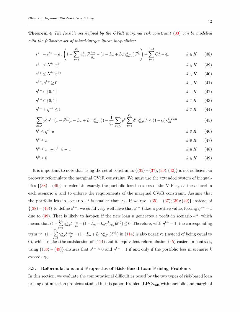
Theorem 4 The feasible set defined by the CVaR marginal risk constraint (33) can be modelled

with the following set of mixed-integer linear inequalities:

sk−− sk+ = an

(1−

Tn∑t=1

γkn,tδtxnqn− (1−Ln +Lnγ

kn,Tn

)δt∗n

)+

n−1∑i=1

Oki − qα k ∈K (38)

sk− ≤Nk−ηk− k ∈K (39)

sk+ ≤Nk+ηk+ k ∈K (40)

sk−, sk+ ≥ 0 k ∈K (41)

ηk− ∈ {0,1} k ∈K (42)

ηk+ ∈ {0,1} k ∈K (43)

ηk−+ ηk+ ≤ 1 k ∈K (44)∑k∈K

pkηk−(1− δt∗n(1−Ln +Lnγ

kn,Tn

))− 1

qn

∑k∈K

pkTn∑t=1

δtγkn,thk ≤ (1−α)κCV aRM (45)

hk ≤ ηk−u k ∈K (46)

hk ≤ xn k ∈K (47)

hk ≥ xn + ηk−u−u k ∈K (48)

hk ≥ 0 k ∈K (49)

It is important to note that using the set of constraints {(35)−(37); (39); (42)} is not sufficient to

properly reformulate the marginal CVaR constraint. We must use the extended system of inequal-

ities {(38)− (49)} to calculate exactly the portfolio loss in excess of the VaR qα at the α level in

each scenario k and to enforce the requirements of the marginal CVaR constraint. Assume that

the portfolio loss in scenario ωk is smaller than qα. If we use {(35)− (37); (39); (42)} instead of

{(38)− (49)} to define sk−, we could very well have that sk− takes a positive value, forcing ηk− = 1

due to (39). That is likely to happen if the new loan n generates a profit in scenario ωk, which

means that (1−Tn∑t=1

γkn,tδt xnqn−(1−Ln+Lnγ

kn,Tn

)δt∗n)≤ 0. Therefore, with ηk− = 1, the corresponding

term ηk−(1−Tn∑t=1

γkn,tδt xnqn− (1−Ln+Lnγ

kn,Tn

)δt∗n) in (114) is also negative (instead of being equal to

0), which makes the satisfaction of (114) and its equivalent reformulation (45) easier. In contrast,

using {(38)− (49)} ensures that sk− ≥ 0 and ηk− = 1 if and only if the portfolio loss in scenario k

exceeds qα.

3.3. Reformulations and Properties of Risk-Based Loan Pricing Problems

In this section, we evaluate the computational difficulties posed by the two types of risk-based loan

pricing optimization problems studied in this paper. Problem LPOVaR with portfolio and marginal

14

VaR constraints

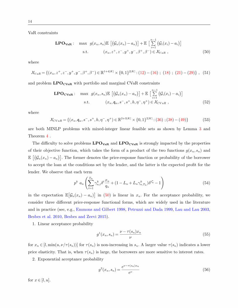
LPOVaR : max g(xn, sn)E[(Gn(xn)− an

)]+E

[ n−1∑i=1

(Gi(xi)− ai

)]s.t. (xn, z

+, z−, y+, y−, β+, β−)∈XV aR , (50)

where

XV aR = {(xn, z+, z−, y+, y−, β+, β−)∈R1+4|K|×{0,1}2|K| : (12)− (16) ; (18) ; (21)− (29)} , (51)

and problem LPOCVaR with portfolio and marginal CVaR constraints

LPOCVaR : max g(xn, sn)E[(Gn(xn)− an

)]+E

[ n−1∑i=1

(Gi(xi)− ai

)]s.t. (xn,qα, s

−, s+, h, η−, η+)∈XCV aR , (52)

where

XCV aR = {(xn,qα, s−, s+, h, η−, η+)∈R2+3|K|×{0,1}2|K| : (36) ; (38)− (49)} (53)

are both MINLP problems with mixed-integer linear feasible sets as shown by Lemma 3 and

Theorem 4 .

The difficulty to solve problems LPOVaR and LPOCVaR is strongly impacted by the properties

of their objective function, which takes the form of a product of the two functions g(xn, sn) and

E[(Gn(xn)− an

)]. The former denotes the price-response function or probability of the borrower

to accept the loan at the conditions set by the lender, and the latter is the expected profit for the

lender. We observe that each term

pk an

(Tn∑t=1

γkn,tδtxnqn

+ (1−Ln +Lnγkn,Tn

)δt∗n − 1

)(54)

in the expectation E[Gn(xn) − an)

]in (50) is linear in xn. For the acceptance probability, we

consider three different price-response functional forms, which are widely used in the literature

and in practice (see, e.g., Emmons and Gilbert 1998, Petruzzi and Dada 1999, Lau and Lau 2003,

Besbes et al. 2010, Besbes and Zeevi 2015).

1. Linear acceptance probability

g1(xn, sn) =ν− τ(sn)xn

ν(55)

for xn ∈ [l,min(u, ν/τ(sn))] for τ(sn) is non-increasing in sn. A larger value τ(sn) indicates a lower

price elasticity. That is, when τ(sn) is large, the borrowers are more sensitive to interest rates.

2. Exponential acceptance probability

g2(xn, sn) =eν−τ(sn)xn

eν(56)

for x∈ [l, u].

Chun and Lejeune: Risk-based Loan Pricing

15

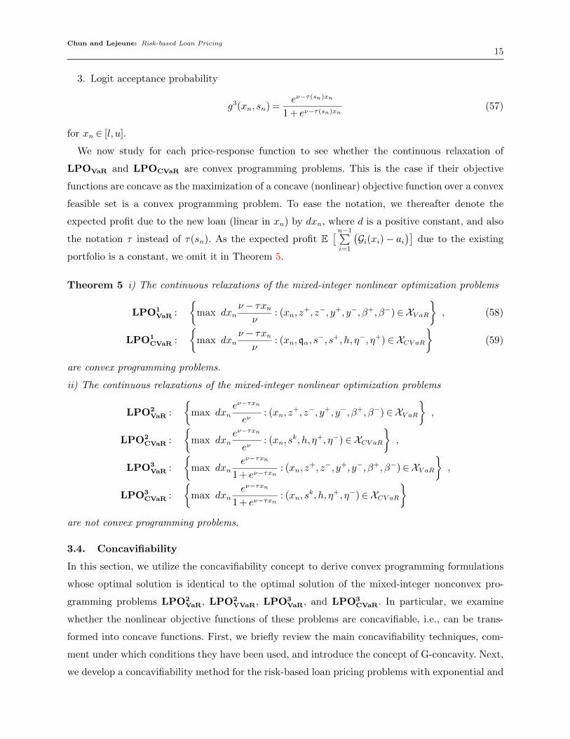
3. Logit acceptance probability

g3(xn, sn) =eν−τ(sn)xn

1 + eν−τ(sn)xn(57)

for xn ∈ [l, u].

We now study for each price-response function to see whether the continuous relaxation of

LPOVaR and LPOCVaR are convex programming problems. This is the case if their objective

functions are concave as the maximization of a concave (nonlinear) objective function over a convex

feasible set is a convex programming problem. To ease the notation, we thereafter denote the

expected profit due to the new loan (linear in xn) by dxn, where d is a positive constant, and also

the notation τ instead of τ(sn). As the expected profit E[ n−1∑i=1

(Gi(xi)− ai

)]due to the existing

portfolio is a constant, we omit it in Theorem 5.

Theorem 5 i) The continuous relaxations of the mixed-integer nonlinear optimization problems

LPO1VaR :

{max dxn

ν− τxnν

: (xn, z+, z−, y+, y−, β+, β−)∈XV aR

}, (58)

LPO1CVaR :

{max dxn

ν− τxnν

: (xn,qα, s−, s+, h, η−, η+)∈XCV aR

}(59)

are convex programming problems.

ii) The continuous relaxations of the mixed-integer nonlinear optimization problems

LPO2VaR :

{max dxn

eν−τxn

eν: (xn, z

+, z−, y+, y−, β+, β−)∈XV aR},

LPO2CVaR :

{max dxn

eν−τxn

eν: (xn, s

k, h, η+, η−)∈XCV aR},

LPO3VaR :

{max dxn

eν−τxn

1 + eν−τxn: (xn, z

+, z−, y+, y−, β+, β−)∈XV aR},

LPO3CVaR :

{max dxn

eν−τxn

1 + eν−τxn: (xn, s

k, h, η+, η−)∈XCV aR}

are not convex programming problems.

3.4. Concavifiability

In this section, we utilize the concavifiability concept to derive convex programming formulations

whose optimal solution is identical to the optimal solution of the mixed-integer nonconvex pro-

gramming problems LPO2VaR, LPO2

VVaR, LPO3VaR, and LPO3

CVaR. In particular, we examine

whether the nonlinear objective functions of these problems are concavifiable, i.e., can be trans-

formed into concave functions. First, we briefly review the main concavifiability techniques, com-

ment under which conditions they have been used, and introduce the concept of G-concavity. Next,

we develop a concavifiability method for the risk-based loan pricing problems with exponential and

16

logit willingness-to-pay functions and derive the resulting convex programming formulations for

the continuous relaxations of these problems.

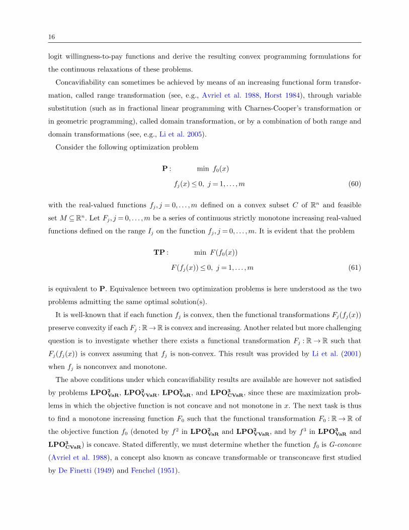
Concavifiability can sometimes be achieved by means of an increasing functional form transfor-

mation, called range transformation (see, e.g., Avriel et al. 1988, Horst 1984), through variable

substitution (such as in fractional linear programming with Charnes-Cooper’s transformation or

in geometric programming), called domain transformation, or by a combination of both range and

domain transformations (see, e.g., Li et al. 2005).

Consider the following optimization problem

P : min f0(x)

fj(x)≤ 0, j = 1, . . . ,m (60)

with the real-valued functions fj, j = 0, . . . ,m defined on a convex subset C of Rn and feasible

set M ⊆Rn. Let Fj, j = 0, . . . ,m be a series of continuous strictly monotone increasing real-valued

functions defined on the range Ij on the function fj, j = 0, . . . ,m. It is evident that the problem

TP : min F (f0(x))

F (fj(x))≤ 0, j = 1, . . . ,m (61)

is equivalent to P. Equivalence between two optimization problems is here understood as the two

problems admitting the same optimal solution(s).

It is well-known that if each function fj is convex, then the functional transformations Fj(fj(x))

preserve convexity if each Fj :R→R is convex and increasing. Another related but more challenging

question is to investigate whether there exists a functional transformation Fj : R→ R such that

Fj(fj(x)) is convex assuming that fj is non-convex. This result was provided by Li et al. (2001)

when fj is nonconvex and monotone.

The above conditions under which concavifiability results are available are however not satisfied

by problems LPO2VaR, LPO2

VVaR, LPO3VaR, and LPO3

CVaR, since these are maximization prob-

lems in which the objective function is not concave and not monotone in x. The next task is thus

to find a monotone increasing function F0 such that the functional transformation F0 : R→ R of

the objective function f0 (denoted by f2 in LPO2VaR and LPO2

VVaR, and by f3 in LPO3VaR and

LPO3CVaR) is concave. Stated differently, we must determine whether the function f0 is G-concave

(Avriel et al. 1988), a concept also known as concave transformable or transconcave first studied

by De Finetti (1949) and Fenchel (1951).

Chun and Lejeune: Risk-based Loan Pricing

17

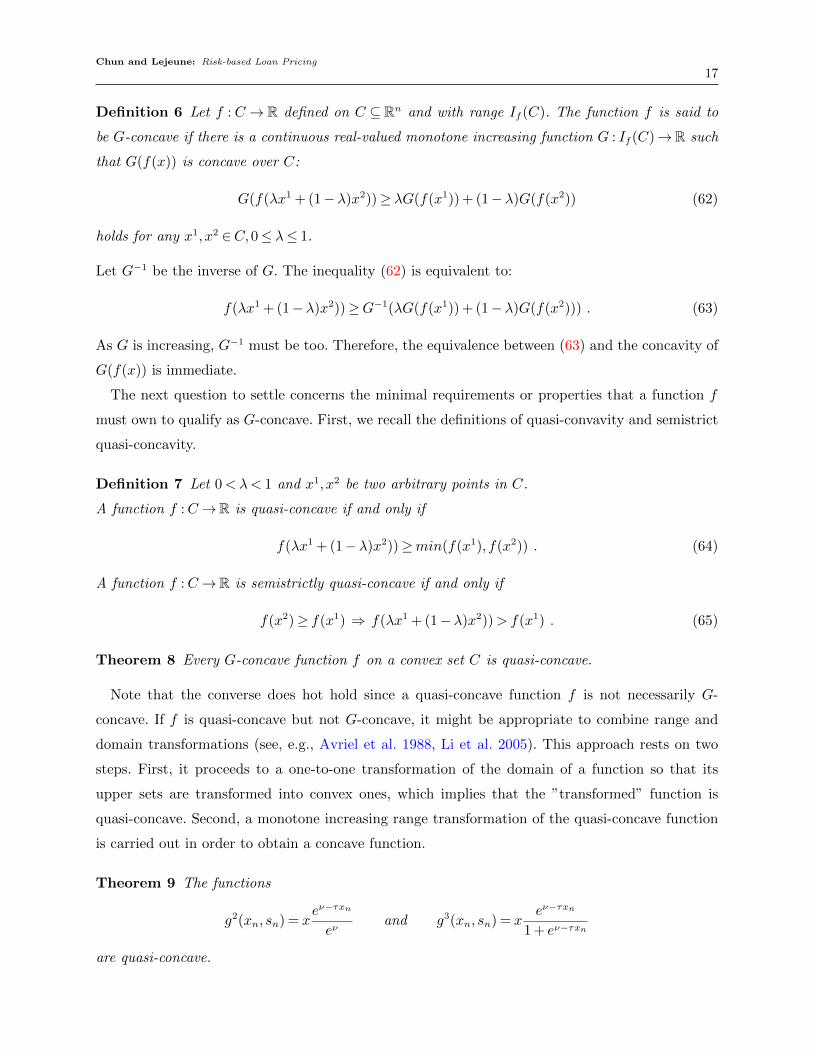
Definition 6 Let f : C→ R defined on C ⊆ Rn and with range If (C). The function f is said to

be G-concave if there is a continuous real-valued monotone increasing function G : If (C)→R such

that G(f(x)) is concave over C:

G(f(λx1 + (1−λ)x2))≥ λG(f(x1)) + (1−λ)G(f(x2)) (62)

holds for any x1, x2 ∈C,0≤ λ≤ 1.

Let G−1 be the inverse of G. The inequality (62) is equivalent to:

f(λx1 + (1−λ)x2))≥G−1(λG(f(x1)) + (1−λ)G(f(x2))) . (63)

As G is increasing, G−1 must be too. Therefore, the equivalence between (63) and the concavity of

G(f(x)) is immediate.

The next question to settle concerns the minimal requirements or properties that a function f

must own to qualify as G-concave. First, we recall the definitions of quasi-convavity and semistrict

quasi-concavity.

Definition 7 Let 0<λ< 1 and x1, x2 be two arbitrary points in C.

A function f :C→R is quasi-concave if and only if

f(λx1 + (1−λ)x2))≥min(f(x1), f(x2)) . (64)

A function f :C→R is semistrictly quasi-concave if and only if

f(x2)≥ f(x1) ⇒ f(λx1 + (1−λ)x2))> f(x1) . (65)

Theorem 8 Every G-concave function f on a convex set C is quasi-concave.

Note that the converse does hot hold since a quasi-concave function f is not necessarily G-

concave. If f is quasi-concave but not G-concave, it might be appropriate to combine range and

domain transformations (see, e.g., Avriel et al. 1988, Li et al. 2005). This approach rests on two

steps. First, it proceeds to a one-to-one transformation of the domain of a function so that its

upper sets are transformed into convex ones, which implies that the ”transformed” function is

quasi-concave. Second, a monotone increasing range transformation of the quasi-concave function

is carried out in order to obtain a concave function.

Theorem 9 The functions

g2(xn, sn) = xeν−τxn

eνand g3(xn, sn) = x

eν−τxn

1 + eν−τxn

are quasi-concave.

18

We shall now demonstrate that the logarithmic function can be used to transform the continuous

relaxations of problems LPO2VaR, LPO2

CVaR, LPO3VaR, and LPO3

CVaR into convex programming

problems.

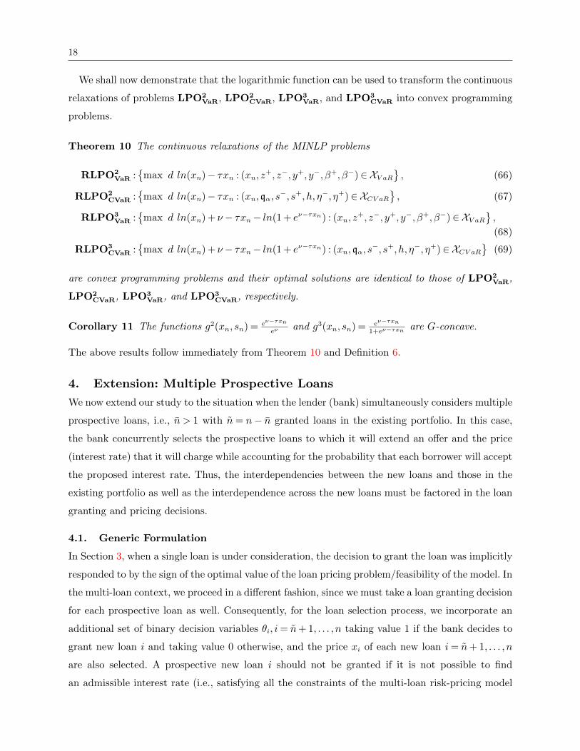
Theorem 10 The continuous relaxations of the MINLP problems

RLPO2VaR :

{max d ln(xn)− τxn : (xn, z

+, z−, y+, y−, β+, β−)∈XV aR}, (66)

RLPO2CVaR :

{max d ln(xn)− τxn : (xn,qα, s

−, s+, h, η−, η+)∈XCV aR}, (67)

RLPO3VaR :

{max d ln(xn) + ν− τxn− ln(1 + eν−τxn) : (xn, z

+, z−, y+, y−, β+, β−)∈XV aR},

(68)

RLPO3CVaR :

{max d ln(xn) + ν− τxn− ln(1 + eν−τxn) : (xn,qα, s

−, s+, h, η−, η+)∈XCV aR}

(69)

are convex programming problems and their optimal solutions are identical to those of LPO2VaR,

LPO2CVaR, LPO3

VaR, and LPO3CVaR, respectively.

Corollary 11 The functions g2(xn, sn) = eν−τxneν

and g3(xn, sn) = eν−τxn1+eν−τxn are G-concave.

The above results follow immediately from Theorem 10 and Definition 6.

4. Extension: Multiple Prospective Loans

We now extend our study to the situation when the lender (bank) simultaneously considers multiple

prospective loans, i.e., n > 1 with n= n− n granted loans in the existing portfolio. In this case,

the bank concurrently selects the prospective loans to which it will extend an offer and the price

(interest rate) that it will charge while accounting for the probability that each borrower will accept

the proposed interest rate. Thus, the interdependencies between the new loans and those in the

existing portfolio as well as the interdependence across the new loans must be factored in the loan

granting and pricing decisions.

4.1. Generic Formulation

In Section 3, when a single loan is under consideration, the decision to grant the loan was implicitly

responded to by the sign of the optimal value of the loan pricing problem/feasibility of the model. In

the multi-loan context, we proceed in a different fashion, since we must take a loan granting decision

for each prospective loan as well. Consequently, for the loan selection process, we incorporate an

additional set of binary decision variables θi, i= n+ 1, . . . , n taking value 1 if the bank decides to

grant new loan i and taking value 0 otherwise, and the price xi of each new loan i= n+ 1, . . . , n

are also selected. A prospective new loan i should not be granted if it is not possible to find

an admissible interest rate (i.e., satisfying all the constraints of the multi-loan risk-pricing model

Chun and Lejeune: Risk-based Loan Pricing

19

introduced below) that leads to a positive profit expected value for loan i. Clearly, from equation

(54), if it is not possible to find xi such that

ai∑k∈K

pk

(Ti∑t=1

γki,tδtxiqi

+ (1−Li +Liγki,Ti

)δt∗i − 1

)≥ 0 , (70)

then loan i should not be granted, since granting it would lead to a negative profit expected value

and be detrimental to the profitability of the bank (and to the value of the objective function). If

the bank does not extend an offer for a new loan, we have that θi = 0 = ζi. The random loss of a

portfolio is ζ =n∑i=1

ζi, where ζi = ai−Gi, i= 1 . . . , n is the random loss due to a loan in the existing

portfolio and ζi = θi(ai−Gi), i= n+ 1, . . . , n, is the random loss due to a prospective new loan. As

explained below, the loan selection process introduces additional combinatorics and nonconvexity

elements that further compound the complexity of the loan pricing problem.

The generic formulation of the risk-based loan pricing model LPO-M with simultaneous con-

sideration of multiple loans can be written as:

LPO-M :

maxxn+1,...,xn,θ

{h(xn+1, . . . , xn, θ) :=

n∑i=n+1

θig(xi, si)E[(Gi(xi)− ai

)]+E

[ n∑i=1

(Gi(xi)− ai

)]}(71)

s.t. l≤ xi ≤ u, i= n+ 1, . . . , n (72)

ρMi (ζ(xn+1, . . . , xn, θ)) ≤ κMai, i= n+ 1, . . . , n (73)

ρ (ζ(xn+1, . . . , xn, θ)) ≤ κP

n∑i=1

ai . (74)

The objective (71) is to maximize the expected profit taking into account uncertainties in both the

borrowers’ reaction to the proposed interest rate and the default risk. Constraints (72) underline

that a price must be determined for each prospective loan. The inequalities (73) and (74) represent

the n marginal and the portfolio risk constraints with respective risk thresholds κM and κP .

In the next section, we develop the explicit mathematical formulations of the multi-loan risk-

pricing problems with VaR and CVaR measures, discuss their complexity, and develop reformula-

tions amenable to a numerical solution.

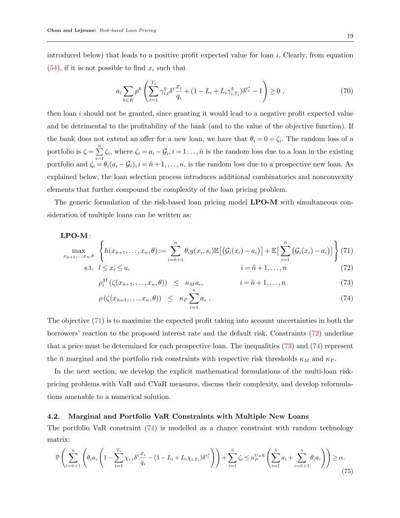
4.2. Marginal and Portfolio VaR Constraints with Multiple New Loans

The portfolio VaR constraint (74) is modelled as a chance constraint with random technology

matrix:

P

(n∑

i=n+1

(θiai

(1−

Ti∑t=1

χi,tδtxiqi− (1−Li +Liχi,Ti)δ

t∗i

))+

n∑i=1

ζi ≤ κV aRP

(n∑i=1

ai +

n∑i=n+1

θiai

))≥ α.

(75)

20

However, while the stochastic inequality that must hold with probability α is linear in the single loan pricing

problem (6), the stochastic inequality

n∑i=n+1

(θiai

(1−

Ti∑t=1

χi,tδtxiqi− (1−Li +Liχi,Ti)δ

t∗i

))+

n∑i=1

ζi ≤ κV aRP

(n∑i=1

ai +

n∑i=n+1

θiai

)

is nonlinear and includes binary variables and bilinear nonconvex terms θi xi, i = n + 1, . . . , n (see, e.g.,

Lejeune and Margot 2016) in the multi-loan context.

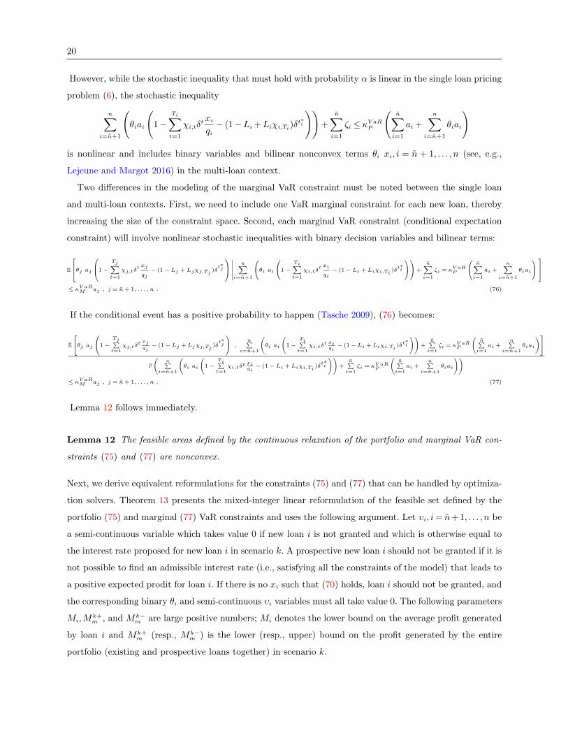
Two differences in the modeling of the marginal VaR constraint must be noted between the single loan

and multi-loan contexts. First, we need to include one VaR marginal constraint for each new loan, thereby

increasing the size of the constraint space. Second, each marginal VaR constraint (conditional expectation

constraint) will involve nonlinear stochastic inequalities with binary decision variables and bilinear terms:

E

θj aj1−

Tj∑t=1

χj,tδt xj

qj− (1−Lj +Ljχj,Tj )δ

t∗j

∣∣∣∣∣∣

n∑i=n+1

θi ai1−

Ti∑t=1

χi,tδt xi

qi− (1−Li +Liχi,Ti )δ

t∗i

+

n∑i=1

ζi = κV aRP

n∑i=1

ai +n∑

i=n+1

θiai

≤ κV aRM aj , j = n+ 1, . . . , n . (76)

If the conditional event has a positive probability to happen (Tasche 2009), (76) becomes:

E

θj aj1−

Tj∑t=1

χj,tδt xjqj− (1−Lj +Ljχj,Tj )δ

t∗j

,n∑

i=n+1

(θi ai

(1−

Ti∑t=1

χi,tδt xiqi− (1−Li +Liχi,Ti )δ

t∗i

))+

n∑i=1

ζi = κV aRP

(n∑i=1

ai +n∑

i=n+1θiai

)P

(n∑

i=n+1

(θi ai

(1−

Ti∑t=1

χi,tδtxiqi− (1−Li +Liχi,Ti )δ

t∗i

))+

n∑i=1

ζi = κV aRP

(n∑i=1

ai +n∑

i=n+1θiai

))≤ κV aRM aj , j = n+ 1, . . . , n . (77)

Lemma 12 follows immediately.

Lemma 12 The feasible areas defined by the continuous relaxation of the portfolio and marginal VaR con-

straints (75) and (77) are nonconvex.

Next, we derive equivalent reformulations for the constraints (75) and (77) that can be handled by optimiza-

tion solvers. Theorem 13 presents the mixed-integer linear reformulation of the feasible set defined by the

portfolio (75) and marginal (77) VaR constraints and uses the following argument. Let υi, i= n+ 1, . . . , n be

a semi-continuous variable which takes value 0 if new loan i is not granted and which is otherwise equal to

the interest rate proposed for new loan i in scenario k. A prospective new loan i should not be granted if it is

not possible to find an admissible interest rate (i.e., satisfying all the constraints of the model) that leads to

a positive expected prodit for loan i. If there is no xi such that (70) holds, loan i should not be granted, and

the corresponding binary θi and semi-continuous υi variables must all take value 0. The following parameters

Mi,Mk+m , and Mk−

m are large positive numbers; Mi denotes the lower bound on the average profit generated

by loan i and Mk+m (resp., Mk−

m ) is the lower (resp., upper) bound on the profit generated by the entire

portfolio (existing and prospective loans together) in scenario k.

Chun and Lejeune: Risk-based Loan Pricing

21

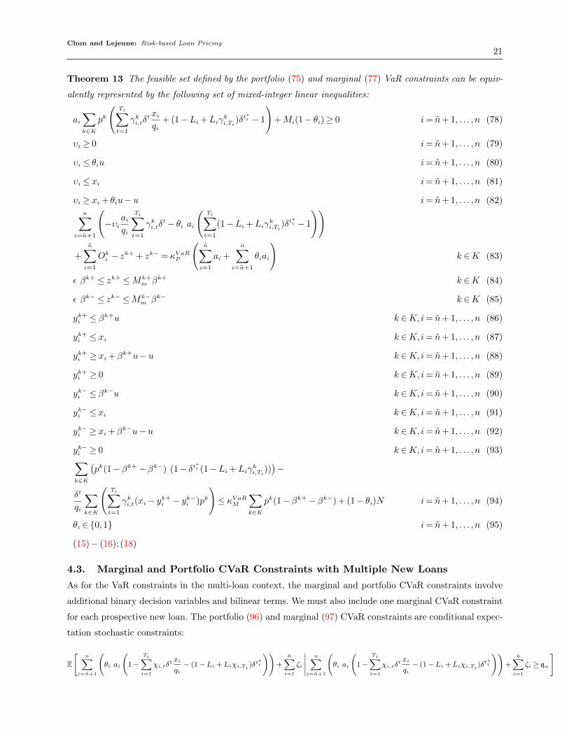
Theorem 13 The feasible set defined by the portfolio (75) and marginal (77) VaR constraints can be equiv-

alently represented by the following set of mixed-integer linear inequalities:

ai∑k∈K

pk

(Ti∑t=1

γki,tδtxiqi

+ (1−Li +Liγki,Ti

)δt∗i − 1

)+Mi(1− θi)≥ 0 i= n+ 1, . . . , n (78)

υi ≥ 0 i= n+ 1, . . . , n (79)

υi ≤ θiu i= n+ 1, . . . , n (80)

υi ≤ xi i= n+ 1, . . . , n (81)

υi ≥ xi + θiu−u i= n+ 1, . . . , n (82)

n∑i=n+1

(−υi

aiqi

Ti∑t=1

γki,tδt− θi ai

(Ti∑t=1

(1−Li +Liγki,Ti

)δt∗i − 1

))

+

n∑i=1

Oki − zk+ + zk− = κV aRP

(n∑i=1

ai +

n∑i=n+1

θiai

)k ∈K (83)

ε βk+ ≤ zk+ ≤Mk+m βk+ k ∈K (84)

ε βk− ≤ zk− ≤Mk−m βk− k ∈K (85)

yk+i ≤ βk+u k ∈K, i= n+ 1, . . . , n (86)

yk+i ≤ xi k ∈K, i= n+ 1, . . . , n (87)

yk+i ≥ xi +βk+u−u k ∈K, i= n+ 1, . . . , n (88)

yk+i ≥ 0 k ∈K, i= n+ 1, . . . , n (89)

yk−i ≤ βk−u k ∈K, i= n+ 1, . . . , n (90)

yk−i ≤ xi k ∈K, i= n+ 1, . . . , n (91)

yk−i ≥ xi +βk−u−u k ∈K, i= n+ 1, . . . , n (92)

yk−i ≥ 0 k ∈K, i= n+ 1, . . . , n (93)∑k∈K

(pk(1−βk+−βk−) (1− δt∗i (1−Li +Liγ

ki,Ti

)))−

δt

qi

∑k∈K

(Ti∑t=1

γki,t(xi− yk+i − yk−i )pk

)≤ κV aRM

∑k∈K

pk(1−βk+−βk−) + (1− θi)N i= n+ 1, . . . , n (94)

θi ∈ {0,1} i= n+ 1, . . . , n (95)

(15)− (16); (18)

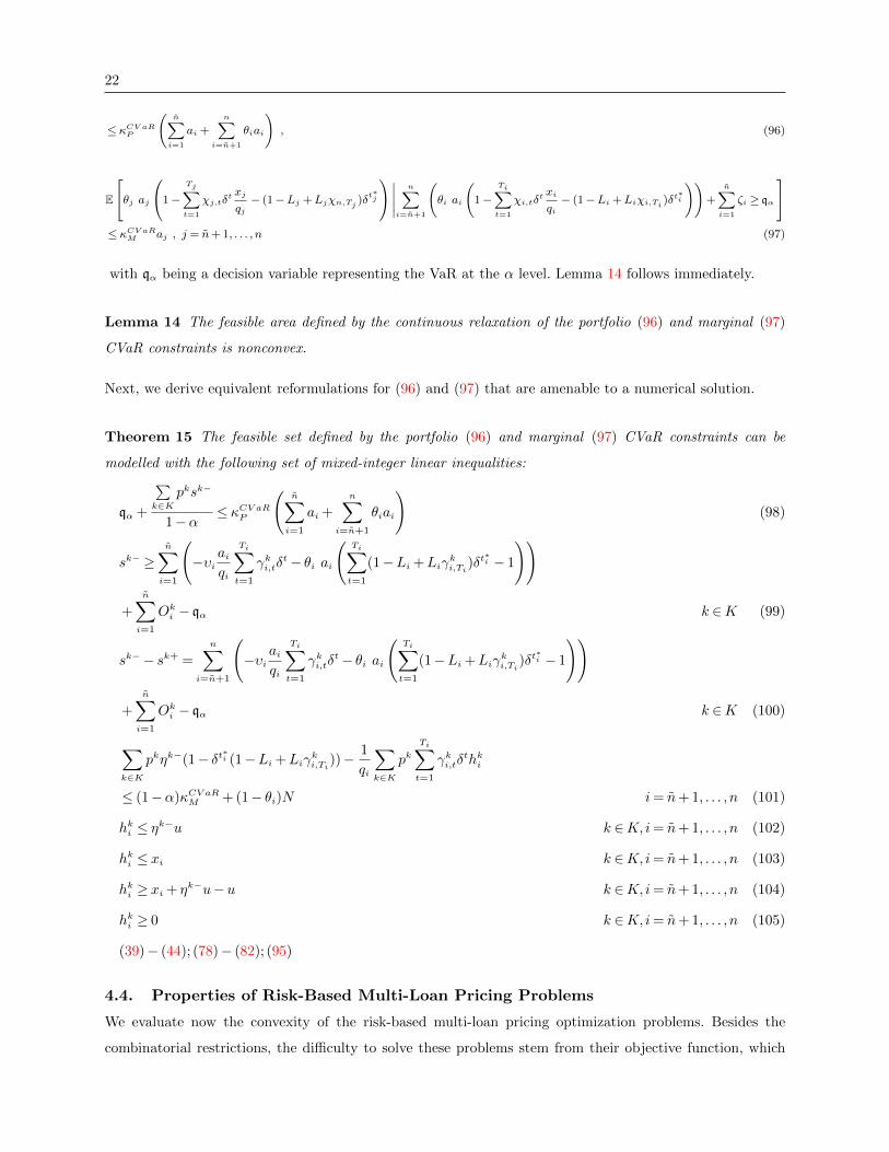
4.3. Marginal and Portfolio CVaR Constraints with Multiple New Loans

As for the VaR constraints in the multi-loan context, the marginal and portfolio CVaR constraints involve

additional binary decision variables and bilinear terms. We must also include one marginal CVaR constraint

for each prospective new loan. The portfolio (96) and marginal (97) CVaR constraints are conditional expec-

tation stochastic constraints:

E

[n∑

i=n+1

(θi ai

(1−

Ti∑t=1

χi,tδt xi

qi− (1−Li+Liχi,Ti )δ

t∗i

))+

n∑i=1

ζi

∣∣∣∣∣n∑

i=n+1

(θi ai

(1−

Ti∑t=1

χi,tδt xi

qi− (1−Li+Liχi,Ti )δ

t∗i

))+

n∑i=1

ζi ≥ qα

]

22

≤ κCV aRP

(n∑i=1

ai+

n∑i=n+1

θiai

), (96)

E

θj aj1−

Tj∑t=1

χj,tδt xj

qj− (1−Lj +Ljχn,Tj )δ

t∗j

∣∣∣∣∣n∑

i=n+1

(θi ai

(1−

Ti∑t=1

χi,tδt xi

qi− (1−Li+Liχi,Ti )δ

t∗i

))+

n∑i=1

ζi ≥ qα

≤ κCV aRM aj , j = n+1, . . . , n (97)

with qα being a decision variable representing the VaR at the α level. Lemma 14 follows immediately.

Lemma 14 The feasible area defined by the continuous relaxation of the portfolio (96) and marginal (97)

CVaR constraints is nonconvex.

Next, we derive equivalent reformulations for (96) and (97) that are amenable to a numerical solution.

Theorem 15 The feasible set defined by the portfolio (96) and marginal (97) CVaR constraints can be

modelled with the following set of mixed-integer linear inequalities:

qα +

∑k∈K

pksk−

1−α≤ κCV aRP

(n∑i=1

ai +

n∑i=n+1

θiai

)(98)

sk− ≥n∑i=1

(−υi

aiqi

Ti∑t=1

γki,tδt− θi ai

(Ti∑t=1

(1−Li +Liγki,Ti

)δt∗i − 1

))

+

n∑i=1

Oki − qα k ∈K (99)

sk−− sk+ =

n∑i=n+1

(−υi

aiqi

Ti∑t=1

γki,tδt− θi ai

(Ti∑t=1

(1−Li +Liγki,Ti

)δt∗i − 1

))

+

n∑i=1

Oki − qα k ∈K (100)

∑k∈K

pkηk−(1− δt∗i (1−Li +Liγki,Ti

))− 1

qi

∑k∈K

pkTi∑t=1

γki,tδthki

≤ (1−α)κCV aRM + (1− θi)N i= n+ 1, . . . , n (101)

hki ≤ ηk−u k ∈K, i= n+ 1, . . . , n (102)

hki ≤ xi k ∈K, i= n+ 1, . . . , n (103)

hki ≥ xi + ηk−u−u k ∈K, i= n+ 1, . . . , n (104)

hki ≥ 0 k ∈K, i= n+ 1, . . . , n (105)

(39)− (44); (78)− (82); (95)

4.4. Properties of Risk-Based Multi-Loan Pricing Problems

We evaluate now the convexity of the risk-based multi-loan pricing optimization problems. Besides the

combinatorial restrictions, the difficulty to solve these problems stem from their objective function, which

Chun and Lejeune: Risk-based Loan Pricing

23

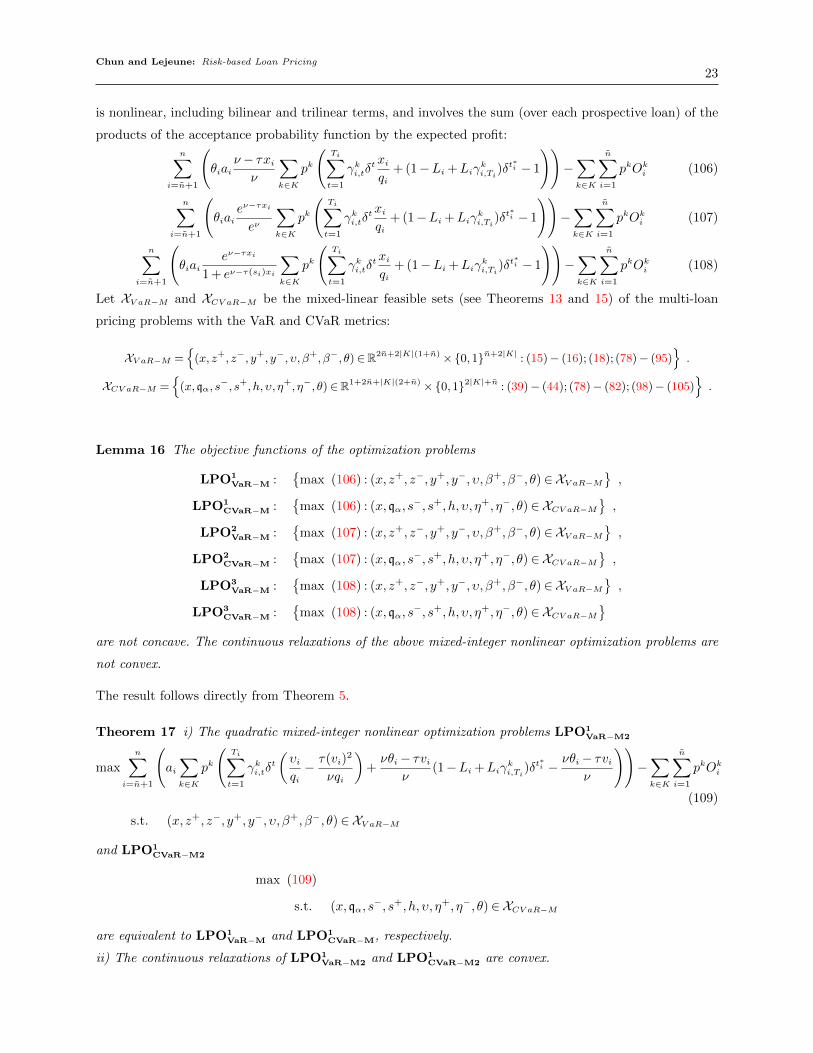
is nonlinear, including bilinear and trilinear terms, and involves the sum (over each prospective loan) of the

products of the acceptance probability function by the expected profit:

n∑i=n+1

(θiai

ν− τxiν

∑k∈K

pk

(Ti∑t=1

γki,tδtxiqi

+ (1−Li +Liγki,Ti

)δt∗i − 1

))−∑k∈K

n∑i=1

pkOki (106)

n∑i=n+1

(θiai

eν−τxi

eν

∑k∈K

pk

(Ti∑t=1

γki,tδtxiqi

+ (1−Li +Liγki,Ti

)δt∗i − 1

))−∑k∈K

n∑i=1

pkOki (107)

n∑i=n+1

(θiai

eν−τxi

1 + eν−τ(si)xi

∑k∈K

pk

(Ti∑t=1

γki,tδtxiqi

+ (1−Li +Liγki,Ti

)δt∗i − 1

))−∑k∈K

n∑i=1

pkOki (108)

Let XV aR−M and XCV aR−M be the mixed-linear feasible sets (see Theorems 13 and 15) of the multi-loan

pricing problems with the VaR and CVaR metrics:

XV aR−M ={

(x, z+, z−, y+, y−, υ, β+, β−, θ)∈R2n+2|K|(1+n)×{0,1}n+2|K| : (15)− (16); (18); (78)− (95)}.

XCV aR−M ={

(x,qα, s−, s+, h, υ, η+, η−, θ)∈R1+2n+|K|(2+n)×{0,1}2|K|+n : (39)− (44); (78)− (82); (98)− (105)

}.

Lemma 16 The objective functions of the optimization problems

LPO1VaR−M :

{max (106) : (x, z+, z−, y+, y−, υ, β+, β−, θ)∈XV aR−M

},

LPO1CVaR−M :

{max (106) : (x,qα, s

−, s+, h, υ, η+, η−, θ)∈XCV aR−M},

LPO2VaR−M :

{max (107) : (x, z+, z−, y+, y−, υ, β+, β−, θ)∈XV aR−M

},

LPO2CVaR−M :

{max (107) : (x,qα, s

−, s+, h, υ, η+, η−, θ)∈XCV aR−M},

LPO3VaR−M :

{max (108) : (x, z+, z−, y+, y−, υ, β+, β−, θ)∈XV aR−M

},

LPO3CVaR−M :

{max (108) : (x,qα, s

−, s+, h, υ, η+, η−, θ)∈XCV aR−M}

are not concave. The continuous relaxations of the above mixed-integer nonlinear optimization problems are

not convex.

The result follows directly from Theorem 5.

Theorem 17 i) The quadratic mixed-integer nonlinear optimization problems LPO1VaR−M2

max

n∑i=n+1

(ai∑k∈K

pk

(Ti∑t=1

γki,tδt

(υiqi− τ(vi)

2

νqi

)+νθi− τvi

ν(1−Li +Liγ

ki,Ti

)δt∗i − νθi− τvi

ν

))−∑k∈K

n∑i=1

pkOki

(109)

s.t. (x, z+, z−, y+, y−, υ, β+, β−, θ)∈XV aR−M

and LPO1CVaR−M2

max (109)

s.t. (x,qα, s−, s+, h, υ, η+, η−, θ)∈XCV aR−M

are equivalent to LPO1VaR−M and LPO1

CVaR−M, respectively.

ii) The continuous relaxations of LPO1VaR−M2 and LPO1

CVaR−M2 are convex.

24

Theorem 9 shows that the objective functions of the single loan risk-pricing problems LPO2VaR−M,

LPO2CVaR−M, LPO3

VaR−M, and LPO3CVaR−M associated with the exponential and logit acceptance proba-

bility functions are quasi-concave, which subsequently allows for their concavifiability. However, in case of

multiple loans, the objective functions involve the sum of quasi-concave functions and it is well-known that

the quasi-concavity property does not carry over the summation operation, which impedes their concavifia-

bility and the derivation of convex continuous relaxations.

5. Illustrative Numerical Examples

In this section, we perform Monte Carlo simulations and present numerical examples to illustrate our results

and provide additional insight. To demonstrate how the marginal risk and price-response (acceptance prob-

ability) considerations could affect the optimal price and the profit (portfolio performance), we first consider

a portfolio with one new loan n= 1, and n− n= n− 1 = 49 (later, we also consider n= 500). Wet qi = 4,

Ti = 20, i = 1,2, . . . n, and vary the loan characteristics by randomly generating xi (for the existing loans

i= 1, . . . , n−1) and ai from uniform distributions: xi ∼U(0.0062,0.0092)12, ai ∼U(400,1200), and Li from a

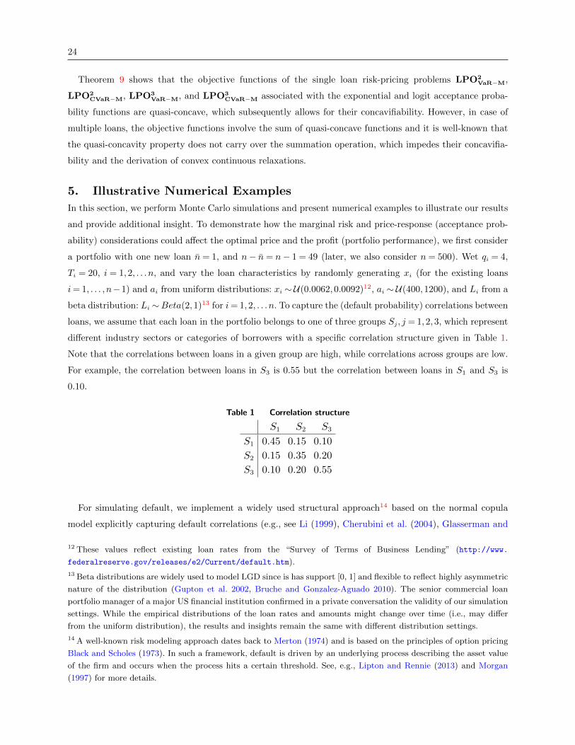
beta distribution: Li ∼Beta(2,1)13 for i= 1,2, . . . n. To capture the (default probability) correlations between

loans, we assume that each loan in the portfolio belongs to one of three groups Sj , j = 1,2,3, which represent

different industry sectors or categories of borrowers with a specific correlation structure given in Table 1.

Note that the correlations between loans in a given group are high, while correlations across groups are low.

For example, the correlation between loans in S3 is 0.55 but the correlation between loans in S1 and S3 is

0.10.

Table 1 Correlation structure

S1 S2 S3

S1 0.45 0.15 0.10

S2 0.15 0.35 0.20

S3 0.10 0.20 0.55

For simulating default, we implement a widely used structural approach14 based on the normal copula

model explicitly capturing default correlations (e.g., see Li (1999), Cherubini et al. (2004), Glasserman and

12 These values reflect existing loan rates from the “Survey of Terms of Business Lending” (http://www.

federalreserve.gov/releases/e2/Current/default.htm).

13 Beta distributions are widely used to model LGD since is has support [0, 1] and flexible to reflect highly asymmetric

nature of the distribution (Gupton et al. 2002, Bruche and Gonzalez-Aguado 2010). The senior commercial loan

portfolio manager of a major US financial institution confirmed in a private conversation the validity of our simulation

settings. While the empirical distributions of the loan rates and amounts might change over time (i.e., may differ

from the uniform distribution), the results and insights remain the same with different distribution settings.

14 A well-known risk modeling approach dates back to Merton (1974) and is based on the principles of option pricing

Black and Scholes (1973). In such a framework, default is driven by an underlying process describing the asset value

of the firm and occurs when the process hits a certain threshold. See, e.g., Lipton and Rennie (2013) and Morgan

(1997) for more details.

Chun and Lejeune: Risk-based Loan Pricing

25

Li (2005), Glasserman et al. (2008)) as follows. Let pi,t be the marginal probability that the ith loan defaults

at time t and Di,t be the default indicator taking value 1 if ith loan defaults at time t and value 0, otherwise.

In the normal copula model, correlation between the default indicators is captured through a multivariate

normal vector Z = (Z1,Z2, . . . ,Zn) of latent variables (we use the correlation matrix based on the structure

in Table 1) where Di,t = 1{Zi,t > zi,t}, i= 1, . . . , n, and the thresholds zi,t are chosen to match the marginal

default probability pi,t. The marginal default probabilities used in our simulation are based on credit ratings

and credit quality migration (upgrades or downgrades), which is modeled with transition rates estimated

from historical data of credit qualities. We consider eight credit rating categories (AAA, AA, A, BBB, BB,

B, CCC, and D), where AAA corresponds to the highest credit quality and D represents default. We set

the marginal default probabilities for each loan with a specific rating from the credit transition matrices

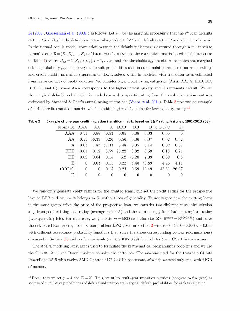
estimated by Standard & Poor’s annual rating migrations (Vazza et al. 2014). Table 2 presents an example

of such a credit transition matrix, which exhibits higher default risk for lower quality ratings15.

Table 2 Example of one-year credit migration transition matrix based on S&P rating histories, 1981-2013 (%).

From/To AAA AA A BBB BB B CCC/C D

AAA 87.1 8.88 0.53 0.05 0.08 0.03 0.05 0

AA 0.55 86.39 8.26 0.56 0.06 0.07 0.02 0.02

A 0.03 1.87 87.33 5.48 0.35 0.14 0.02 0.07

BBB 0.01 0.12 3.59 85.22 3.82 0.59 0.13 0.21

BB 0.02 0.04 0.15 5.2 76.28 7.09 0.69 0.8

B 0 0.03 0.11 0.22 5.48 73.89 4.46 4.11

CCC/C 0 0 0.15 0.23 0.69 13.49 43.81 26.87

D 0 0 0 0 0 0 0 0

We randomly generate credit ratings for the granted loans, but set the credit rating for the prospective

loan as BBB and assume it belongs to S3 without loss of generality. To investigate how the existing loans

in the same group affect the price of the prospective loan, we consider two different cases: the solution

x∗n,G from good existing loan rating (average rating A) and the solution x∗n,B from bad existing loan rating

(average rating BB). For each case, we generate m = 5000 scenarios (i.e. Z ∈ Rm×n = R5000×50) and solve

the risk-based loan pricing optimization problem LPO given in Section 2 with δ = 0.995, l= 0.006, u= 0.011

with different acceptance probability functions (i.e., solve the three corresponding convex reformulations)

discussed in Section 3.3 and confidence levels (α= 0.9,0.95,0.99) for both VaR and CVaR risk measures.

The AMPL modeling language is used to formulate the mathematical programming problems and we use

the Cplex 12.6.1 and Bonmin solvers to solve the instances. The machine used for the tests is a 64 bits

PowerEdge R515 with twelve AMD Opteron 4176 2.4GHz processors, of which we used only one, with 64GB

of memory.

15 Recall that we set qi = 4 and Ti = 20. Thus, we utilize multi-year transition matrices (one-year to five year) as

sources of cumulative probabilities of default and interpolate marginal default probabilities for each time period.

26

Implication of Marginal and Portfolio Risk Consideration. To demonstrate the impact of the

marginal and portfolio risk constraints, we consider the case with standalone VaR and CVaR constraints as

benchmark:

• Standalone VaR constraint:

P

(an

(1−

Tn∑t=1

χn,tδtxnqn− (1−Ln +Lnχn,Tn)δt

∗n

)+

n−1∑i=1

ζi ≤ κV aRS an

)≥ α, (110)

• Standalone CVaR constraint:

E[an

(1−

Tn∑t=1

χn,tδt xnqn− (1−Ln +Lnχn,Tn)δt

∗n

)∣∣∣∣an(1−Tn∑t=1

χn,tδt xnqn− (1−Ln +Lnχn,Tn)δt

∗n

)≥ qαn

]≤ κCV aRS an, (111)

where κS is the standalone risk threshold and qαn is the VaR of the new loan at the α confidence level.

We reformulate and solve the risk-pricing problems M-LPO and S-LPO that respectively include a

marginal and a standalone risk constraint with different levels of κM and κS16:

M−LPO : max (3)

s.t. (4); (33) .

S−LPO : max (3)

s.t. (4); (111) .

Comparing optimal solutions x∗n,G and x∗n,B , we should expect x∗n,G < x∗n,B under the problem with the

marginal risk constraint (M-LPO), but x∗n,G = x∗n,B under the problem with the standalone constraint

(S-LPO).

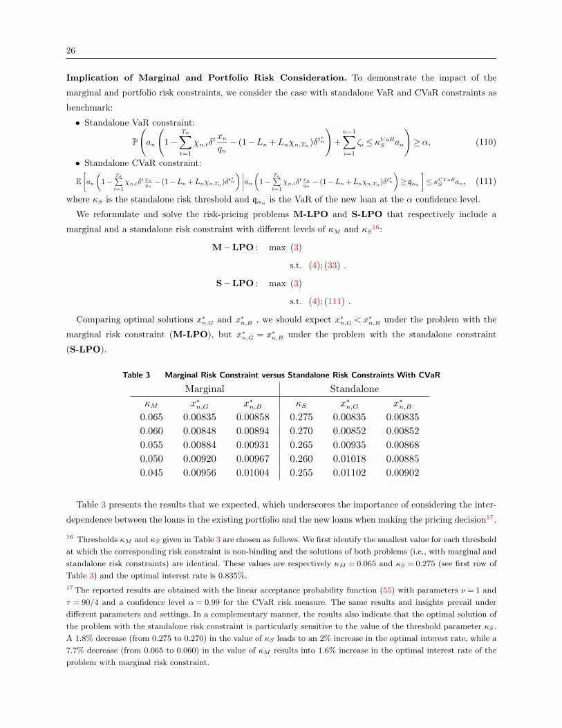
Table 3 Marginal Risk Constraint versus Standalone Risk Constraints With CVaR

Marginal Standalone

κM x∗n,G x∗n,B κS x∗n,G x∗n,B0.065 0.00835 0.00858 0.275 0.00835 0.00835

0.060 0.00848 0.00894 0.270 0.00852 0.00852

0.055 0.00884 0.00931 0.265 0.00935 0.00868

0.050 0.00920 0.00967 0.260 0.01018 0.00885

0.045 0.00956 0.01004 0.255 0.01102 0.00902

Table 3 presents the results that we expected, which underscores the importance of considering the inter-

dependence between the loans in the existing portfolio and the new loans when making the pricing decision17.

16 Thresholds κM and κS given in Table 3 are chosen as follows. We first identify the smallest value for each threshold

at which the corresponding risk constraint is non-binding and the solutions of both problems (i.e., with marginal and

standalone risk constraints) are identical. These values are respectively κM = 0.065 and κS = 0.275 (see first row of

Table 3) and the optimal interest rate is 0.835%.

17 The reported results are obtained with the linear acceptance probability function (55) with parameters ν = 1 and

τ = 90/4 and a confidence level α = 0.99 for the CVaR risk measure. The same results and insights prevail under

different parameters and settings. In a complementary manner, the results also indicate that the optimal solution of

the problem with the standalone risk constraint is particularly sensitive to the value of the threshold parameter κS .

A 1.8% decrease (from 0.275 to 0.270) in the value of κS leads to an 2% increase in the optimal interest rate, while a

7.7% decrease (from 0.065 to 0.060) in the value of κM results into 1.6% increase in the optimal interest rate of the

problem with marginal risk constraint.

Chun and Lejeune: Risk-based Loan Pricing

27

We observe the same result when we solve the following problem P-LPO that includes a portfolio risk

constraint (30):

P−LPO : max (3)

s.t. (4); (32) .

That is, by considering the marginal or portfolio constraint, the lender can take into account the quality

of the existing loans as well as the interdependence between existing loans and the prospective loan when

making pricing decisions.

However, there is a subtle different between the marginal and portfolio risk constraints. To illustrate this,

we solve problem P-LPO, in which we add a marginal risk constraint with fixed marginal risk threshold

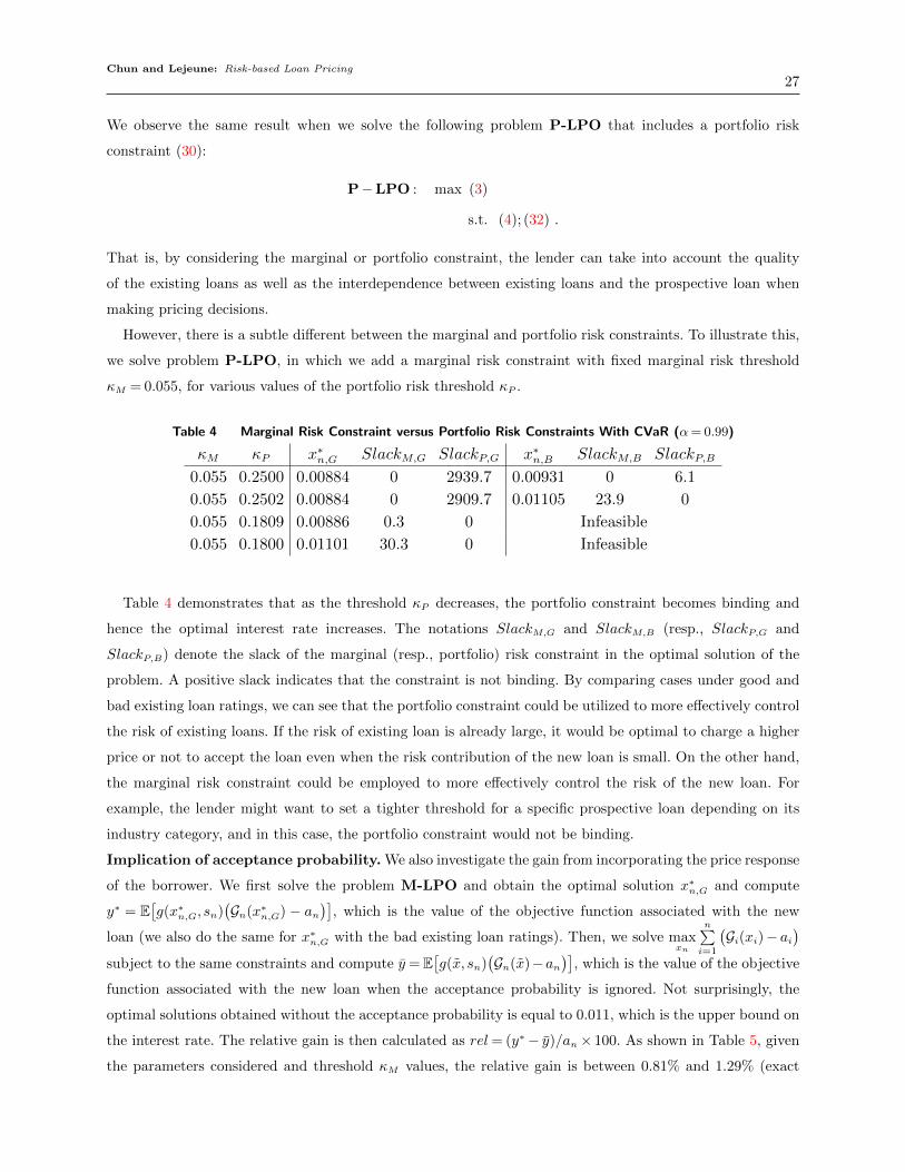
κM = 0.055, for various values of the portfolio risk threshold κP .

Table 4 Marginal Risk Constraint versus Portfolio Risk Constraints With CVaR (α= 0.99)

κM κP x∗n,G SlackM,G SlackP,G x∗n,B SlackM,B SlackP,B

0.055 0.2500 0.00884 0 2939.7 0.00931 0 6.1

0.055 0.2502 0.00884 0 2909.7 0.01105 23.9 0

0.055 0.1809 0.00886 0.3 0 Infeasible

0.055 0.1800 0.01101 30.3 0 Infeasible

Table 4 demonstrates that as the threshold κP decreases, the portfolio constraint becomes binding and

hence the optimal interest rate increases. The notations SlackM,G and SlackM,B (resp., SlackP,G and

SlackP,B) denote the slack of the marginal (resp., portfolio) risk constraint in the optimal solution of the

problem. A positive slack indicates that the constraint is not binding. By comparing cases under good and

bad existing loan ratings, we can see that the portfolio constraint could be utilized to more effectively control

the risk of existing loans. If the risk of existing loan is already large, it would be optimal to charge a higher

price or not to accept the loan even when the risk contribution of the new loan is small. On the other hand,

the marginal risk constraint could be employed to more effectively control the risk of the new loan. For

example, the lender might want to set a tighter threshold for a specific prospective loan depending on its

industry category, and in this case, the portfolio constraint would not be binding.

Implication of acceptance probability. We also investigate the gain from incorporating the price response

of the borrower. We first solve the problem M-LPO and obtain the optimal solution x∗n,G and compute

y∗ = E[g(x∗n,G, sn)

(Gn(x∗n,G) − an

)], which is the value of the objective function associated with the new

loan (we also do the same for x∗n,G with the bad existing loan ratings). Then, we solve maxxn

n∑i=1

(Gi(xi)− ai

)subject to the same constraints and compute y=E

[g(x, sn)

(Gn(x)−an

)], which is the value of the objective

function associated with the new loan when the acceptance probability is ignored. Not surprisingly, the

optimal solutions obtained without the acceptance probability is equal to 0.011, which is the upper bound on

the interest rate. The relative gain is then calculated as rel= (y∗− y)/an× 100. As shown in Table 5, given

the parameters considered and threshold κM values, the relative gain is between 0.81% and 1.29% (exact

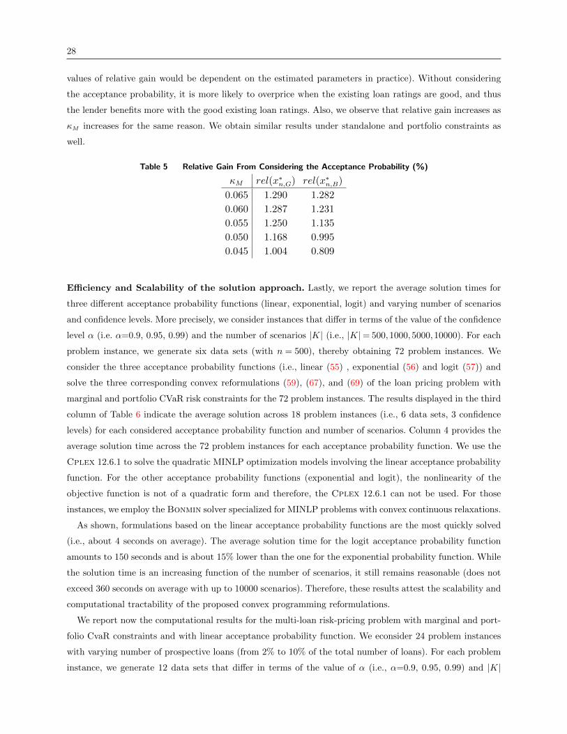
28

values of relative gain would be dependent on the estimated parameters in practice). Without considering

the acceptance probability, it is more likely to overprice when the existing loan ratings are good, and thus

the lender benefits more with the good existing loan ratings. Also, we observe that relative gain increases as

κM increases for the same reason. We obtain similar results under standalone and portfolio constraints as

well.

Table 5 Relative Gain From Considering the Acceptance Probability (%)

κM rel(x∗n,G) rel(x∗n,B)

0.065 1.290 1.282

0.060 1.287 1.231

0.055 1.250 1.135

0.050 1.168 0.995

0.045 1.004 0.809

Efficiency and Scalability of the solution approach. Lastly, we report the average solution times for

three different acceptance probability functions (linear, exponential, logit) and varying number of scenarios

and confidence levels. More precisely, we consider instances that differ in terms of the value of the confidence

level α (i.e. α=0.9, 0.95, 0.99) and the number of scenarios |K| (i.e., |K|= 500,1000,5000,10000). For each

problem instance, we generate six data sets (with n = 500), thereby obtaining 72 problem instances. We

consider the three acceptance probability functions (i.e., linear (55) , exponential (56) and logit (57)) and

solve the three corresponding convex reformulations (59), (67), and (69) of the loan pricing problem with

marginal and portfolio CVaR risk constraints for the 72 problem instances. The results displayed in the third

column of Table 6 indicate the average solution across 18 problem instances (i.e., 6 data sets, 3 confidence

levels) for each considered acceptance probability function and number of scenarios. Column 4 provides the

average solution time across the 72 problem instances for each acceptance probability function. We use the

Cplex 12.6.1 to solve the quadratic MINLP optimization models involving the linear acceptance probability

function. For the other acceptance probability functions (exponential and logit), the nonlinearity of the

objective function is not of a quadratic form and therefore, the Cplex 12.6.1 can not be used. For those

instances, we employ the Bonmin solver specialized for MINLP problems with convex continuous relaxations.

As shown, formulations based on the linear acceptance probability functions are the most quickly solved

(i.e., about 4 seconds on average). The average solution time for the logit acceptance probability function

amounts to 150 seconds and is about 15% lower than the one for the exponential probability function. While

the solution time is an increasing function of the number of scenarios, it still remains reasonable (does not

exceed 360 seconds on average with up to 10000 scenarios). Therefore, these results attest the scalability and

computational tractability of the proposed convex programming reformulations.

We report now the computational results for the multi-loan risk-pricing problem with marginal and port-

folio CvaR constraints and with linear acceptance probability function. We econsider 24 problem instances

with varying number of prospective loans (from 2% to 10% of the total number of loans). For each problem

instance, we generate 12 data sets that differ in terms of the value of α (i.e., α=0.9, 0.95, 0.99) and |K|

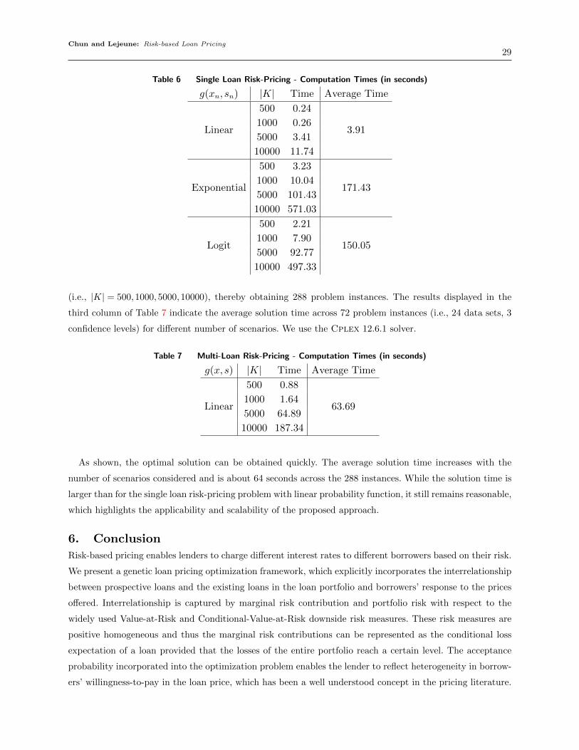
Chun and Lejeune: Risk-based Loan Pricing

29

Table 6 Single Loan Risk-Pricing - Computation Times (in seconds)

g(xn, sn) |K| Time Average Time

Linear

500 0.24

3.911000 0.26

5000 3.41

10000 11.74

Exponential

500 3.23

171.431000 10.04

5000 101.43

10000 571.03

Logit

500 2.21

150.051000 7.90

5000 92.77

10000 497.33

(i.e., |K| = 500,1000,5000,10000), thereby obtaining 288 problem instances. The results displayed in the

third column of Table 7 indicate the average solution time across 72 problem instances (i.e., 24 data sets, 3

confidence levels) for different number of scenarios. We use the Cplex 12.6.1 solver.

Table 7 Multi-Loan Risk-Pricing - Computation Times (in seconds)

g(x, s) |K| Time Average Time

Linear

500 0.88

63.691000 1.64

5000 64.89

10000 187.34

As shown, the optimal solution can be obtained quickly. The average solution time increases with the

number of scenarios considered and is about 64 seconds across the 288 instances. While the solution time is

larger than for the single loan risk-pricing problem with linear probability function, it still remains reasonable,

which highlights the applicability and scalability of the proposed approach.

6. Conclusion

Risk-based pricing enables lenders to charge different interest rates to different borrowers based on their risk.

We present a genetic loan pricing optimization framework, which explicitly incorporates the interrelationship

between prospective loans and the existing loans in the loan portfolio and borrowers’ response to the prices

offered. Interrelationship is captured by marginal risk contribution and portfolio risk with respect to the

widely used Value-at-Risk and Conditional-Value-at-Risk downside risk measures. These risk measures are

positive homogeneous and thus the marginal risk contributions can be represented as the conditional loss

expectation of a loan provided that the losses of the entire portfolio reach a certain level. The acceptance

probability incorporated into the optimization problem enables the lender to reflect heterogeneity in borrow-

ers’ willingness-to-pay in the loan price, which has been a well understood concept in the pricing literature.

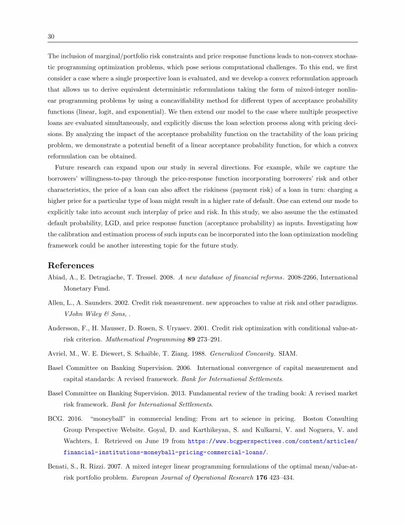
30

The inclusion of marginal/portfolio risk constraints and price response functions leads to non-convex stochas-

tic programming optimization problems, which pose serious computational challenges. To this end, we first

consider a case where a single prospective loan is evaluated, and we develop a convex reformulation approach

that allows us to derive equivalent deterministic reformulations taking the form of mixed-integer nonlin-

ear programming problems by using a concavifiability method for different types of acceptance probability

functions (linear, logit, and exponential). We then extend our model to the case where multiple prospective

loans are evaluated simultaneously, and explicitly discuss the loan selection process along with pricing deci-

sions. By analyzing the impact of the acceptance probability function on the tractability of the loan pricing

problem, we demonstrate a potential benefit of a linear acceptance probability function, for which a convex

reformulation can be obtained.

Future research can expand upon our study in several directions. For example, while we capture the

borrowers’ willingness-to-pay through the price-response function incorporating borrowers’ risk and other

characteristics, the price of a loan can also affect the riskiness (payment risk) of a loan in turn: charging a

higher price for a particular type of loan might result in a higher rate of default. One can extend our mode to

explicitly take into account such interplay of price and risk. In this study, we also assume the the estimated

default probability, LGD, and price response function (acceptance probability) as inputs. Investigating how

the calibration and estimation process of such inputs can be incorporated into the loan optimization modeling

framework could be another interesting topic for the future study.

References

Abiad, A., E. Detragiache, T. Tressel. 2008. A new database of financial reforms. 2008-2266, International

Monetary Fund.

Allen, L., A. Saunders. 2002. Credit risk measurement. new approaches to value at risk and other paradigms.

VJohn Wiley & Sons, .

Andersson, F., H. Mausser, D. Rosen, S. Uryasev. 2001. Credit risk optimization with conditional value-at-

risk criterion. Mathematical Programming 89 273–291.

Avriel, M., W. E. Diewert, S. Schaible, T. Ziang. 1988. Generalized Concavity . SIAM.

Basel Committee on Banking Supervision. 2006. International convergence of capital measurement and

capital standards: A revised framework. Bank for International Settlements.

Basel Committee on Banking Supervision. 2013. Fundamental review of the trading book: A revised market

risk framework. Bank for International Settlements.

BCG. 2016. “moneyball” in commercial lending: From art to science in pricing. Boston Consulting

Group Perspective Website. Goyal, D. and Karthikeyan, S. and Kulkarni, V. and Noguera, V. and

Wachters, I. Retrieved on June 19 from https://www.bcgperspectives.com/content/articles/

financial-institutions-moneyball-pricing-commercial-loans/.

Benati, S., R. Rizzi. 2007. A mixed integer linear programming formulations of the optimal mean/value-at-

risk portfolio problem. European Journal of Operational Research 176 423–434.

Chun and Lejeune: Risk-based Loan Pricing

31

Besbes, O., R. Phillips, A. Zeevi. 2010. Testing the validity of a demand model: An operations perspective.

Manufacturing & Service Operations Management 12(1) 162–183.

Besbes, O., A. Zeevi. 2015. On the (surprising) sufficiency of linear models for dynamic pricing with demand

learning. Management Science 61(4) 723–739.

Black, F., M. Scholes. 1973. The pricing of options and corporate liabilities. The journal of political economy

637–654.

Bostic, R.W. 2002. Trends in equal access to credit products. The Impact of Public Policy on Consumer

Credit . Springer, 171–208.

Bruche, M., C. Gonzalez-Aguado. 2010. Recovery rates, default probabilities, and the credit cycle. Journal

of Banking & Finance 34(4) 754–764.

Burer, S.A., A. Letchford. 2012. Non-convex mixed-integer nonlinear programming: A survey. Surveys in

Operations Research and Management Science 17 97–106.

Caufield, S. 2012. Consumer credit pricing. The Oxford Handbook of Pricing Management, Oxford University

Press, Oxford 138–152.

Cherubini, U., E. Luciano, W. Vecchiato. 2004. Copula Methods in Finance. John Wiley & Sons.

Cohen, M. C., N. H. Z. Leung, K. Panchamgam, G. Perakis, A. Smith. 2016. The impact of linear optimization

on promotion planning. Forthcoming in Operations Research .

Cornuejols, G., R. Tutuncu. 2007. Optimization Methods in Finance. Cambridge, UK: Cambridge University

Press.

Cui, X., S. Zhu, D. Li, X. Sun. 2016. Mean-variance portfolio optimization with parameter sensitivity control.

Optimization Methods and Software 31(4) 755–774.

DAmbrosio, C., A. Lodi. 2011. Mixed integer nonlinear programming tools: A practical overview. 4OR 9(4)

329–349.

De Finetti, B. 1949. Sulle stratificazioni convesse. Annali di Matematica Pura ed Applicata 30(1) 123–183.

DeMiguel, V., L. Garlappi, F. J. Nogales, R. Uppal. 2009. A generalized approach to portfolio optimization:

Improving performance by constraining portfolio norms. Management Science 55(5) 798–812.

Dentcheva, D., A. Ruszczynski. 2015. Risk-averse portfolio optimization via stochastic dominance constraints.

Handbook of Financial Econometrics and Statistics. Springer, 2281–2302.

Edelberg, W. 2006. Risk-based pricing of interest rates for consumer loans. Journal of Monetary Economics

53(8) 2283–2298.

Emmons, H., S. M Gilbert. 1998. Note. the role of returns policies in pricing and inventory decisions for

catalogue goods. Management Science 44(2) 276–283.

Fenchel, W. 1951. Convex Cones, Sets and Functions. Mimeographed lecture Notes. Princeton University,

Princeton, NJ, USA.

32

Feng, M., A. Wachter, J. Staum. 2015. Practice algorithms for value-at-risk portfolio optimization problems.

Quantitative Finance Letters 3 1–9.

Glasserman, P. 2006. Measuring marginal risk contributions in credit portfolios. Journal of Computational

Finance 9(2) 1–41.

Glasserman, P., W. Kang, P. Shahabuddin. 2008. Fast simulation of multifactor portfolio credit risk. Oper-

ations Research 56(5) 1200–1217.

Glasserman, P., J. Li. 2005. Importance sampling for portfolio credit risk. Management Science 51(11)

1643–1656.

Gourieroux, C., J. P. Laurent, O. Scaillet. 2000. Sensitivity analysis of values at risk. Journal of Empirical

Finance 7 225–245.

Gross, D., N. Souleles. 2002. Do liquidity constraints and interest rates matter for consumer behavior?

evidence from credit card data. The Quarterly Journal of Economics 117(1) 149–185.

Gupton, G.M., R.M. Stein, A. Salaam, D. Bren. 2002. LOSSCALCTM: Model for predicting loss given

default (LGD). Moodys KMV, New York .

Horst, R. 1984. On the convexification of nonlinear programming problems: An applications-oriented survey.

European Journal of Operations Research 15 382–392.

Huang, B., L. C. Thomas. 2015. The impact of basel accords on the lender’s profitability under different

pricing decisions. Journal of the Operational Research Society 66 1826–1839.

Johnson, R. W. 1992. Legal, social and economic issues in implementing scoring in the united states. J. N.

Crook, D.B. Edelman, L.C. Thomas, eds., Credit Scoring and Credit Control . Oxford University Press,

5–15.

Kalkbrener, M. 2005. An axiomatic approach to capital allocation. Mathematical Finance 15 425–437.

Kalkbrener, M., H. Lotter, L. Overbeck. 2004. Sensible and efficient asset allocation for credit portfolios.

Risk 17 19–24.

Kataoka, S. 1963. A stochastic programming model. Econometrica 31(1-2) 181–196.

Kawas, B., A. Thiele. 2011. Short sales in log-robust portfolio management. European Journal of Operational

Research 215(3) 651–661.

Kimber, Andrew. 2003. Credit Risk: From Transaction to Portfolio Management . Butterworth-Heinemann.

Krokhmal, P., M. Zabarankin, S. Uryasev. 2011. Modeling and optimization of risk. Surveys in Operations

Research and Management Science 16(2) 49–66.

Kurth, A., D. Tasche. 2003. Contributions to credit risk. Risk 16 84–88.

Lau, A. H. L., H.S. Lau. 2003. Effects of a demand-curves shape on the optimal solutions of a multi-echelon

inventory/pricing model. European Journal of Operational Research 147(3) 530–548.

Chun and Lejeune: Risk-based Loan Pricing

33

Lejeune, M.A., F. Margot. 2016. Solving chance constrained problems with random technology matrix and

stochastic quadratic inequalities. Operations Research 64(4) 939–957.

Li, D., X. L. Sun, M. P. Biswal, F. Gao. 2001. Convexification, concavification and monotonization in global

optimization. Annals of Operations Research 105 213–226.

Li, D., Wu Z.-y., J. Lee H.-w., Yang X.-m., Zhang L.-s. 2005. Hidden convex minimization. Journal og Global

Optimization 31 211–233.

Li, D.X. 1999. On default correlation: A copula function approach. Available at SSRN 187289 .

Lipton, A., A. Rennie. 2013. The Oxford Handbook of Credit Derivatives. Oxford University Press, Oxford.

Liu, G. 2015. Simulating risk contributions of credit portfolios. Operations Research 63(1) 104–121.

Magri, S., R. Pico. 2011. The rise of risk-based pricing of mortgage interest rates in italy. Journal of Banking

& Finance 35(5) 1277–1290.

Mausser, H., D. Rosen. 2008. Economic credit capital allocation and risk contributions. Handbooks in

Operations Research & Management Science - Financial Engineering . Eds: Birge J.R., Linetsky V.

Volume 15. Elsevier, 681–726.

McCormick, G. P. 1976. Computability of global solutions to factorable nonconvex programs: Part i convex

underestimating problems. Mathematical Programming 10(1) 147–175.

Mercer, Z. C. 1992. Valuing Financial Institutions. Irwin Professional Pub.

Merino, S., M. A. Nyfeler. 2004. Applying importance sampling for estimating coherent credit risk contri-

butions. Quantitative Finance 4(2) 199–207.

Merton, R. C. 1974. On the pricing of corporate debt: The risk structure of interest rates. The Journal of

finance 29(2) 449–470.

Morgan, J. P. 1997. CreditmetricsTM . Technical Report. New York, J.P. Morgan.

Musto, David K, Nicholas S Souleles. 2006. A portfolio view of consumer credit. Journal of Monetary

Economics 53(1) 59–84.

Oliver, B. V., R. M. Oliver. 2014. Optimal ROE loan pricing with or without adverse selection. Journal of

the Operational Research Society 65(3) 435–442.

Petruzzi, N. C., M. Dada. 1999. Pricing and the newsvendor problem: A review with extensions. Operations

Research 47(2) 183–194.

Phillips, R. 2005. Pricing and Revenue Optimization. Stanford University Press.

Phillips, R. 2013. Optimizing prices for consumer credit. Journal of Revenue and Pricing Management 12

360–377.

Prekopa, A. 1995. Stochastic Programming . Kluwer. Boston, MA.

34

PwC. 2012. Enhancing origination revenue through price optimization modeling. PricewaterhouseCoopers

Website. Retrieved on June 19 from http://www.pwc.com/us/en/consumer-finance/publications/

loan-origination-price-optimization-modeling.html.

Sageworks. 2016. Loan-pricing models: What to consider for loan origination. Sageworks Blog. posted

by Biery, M. E. Retrieved on May 20 from https://www.sageworks.com/blog/post/2016/01/29/

loan-pricing-models-what-banks-need-to-consider.aspx.

Schuermann, Til. 2004. Why were banks better off in the 2001 recession? Current Issues in Economics and

Finance 10(1).

Stanhouse, B., D. Stock. 2008. Managing the risk of loan prepayments and the optimal structure of short

term lending rates. Annals of Finance 4(2) 197–215.

Tasche, D. 2000. Conditional expectation as quantile derivative. Tech. rep.

Tasche, D. 2009. Capital allocation for credit portfolios with kernel estimators. Quantitative Finance 9(5)

581–595.

Thomas, L. C. 2009. Consumer Credit Models. Oxford University.

Vazza, D., N. Kraemer, N.M. Richhariya, A. Debnath, M. Sangoi. 2014. 2013 annual global corporate default

study and rating transitions. Standard and Poors, March 1.

Yu, J.-R., W.-J. Chiou, D.-R. Mu. 2015. A linearized value-at-risk model with transaction costs and short

selling. European Journal of Operational Research 247 872–878.

Zhu, S., D. Li, X. Sun. 2010. Portfolio selection with marginal risk control. The Journal of Computational

Finance 14(1) 3–28.

Chun and Lejeune: Risk-based Loan Pricing

35

Appendix. Proofs

Proof of Theorem 1.

i) Portfolio VaR constraint: Each constraint (12) defines the amount zk−− zk+ by which the loss in scenario

ωk differs from the threshold loss level κV aRP

n∑i=1

ai. Each constraint in (13) (resp., (14)) forces the binary

variable βk+ (resp., βk−) to take value 1 if the corresponding variable zk+ (resp., zk−) is strictly positive.

Since (15) allows at most one variable in each pair (βk+, βk−) to take value 1, it ensues that only one of

zk+ and zk−, k ∈K can be strictly positive and that zk− (resp., zk+) denotes the loss amount below (resp.,

above) the threshold κV aRP

n∑i=1

ai. The expression∑k∈K

pkβk+ is the probability of the set of scenarios with

total losses exceeding κV aRP

n∑i=1

ai. The knapsack constraint (16) stipulates that the sum of the probabilities

of the violated scenarios must not exceed 1 − α. As a result, the feasible set of (8) can be equivalently

represented by the mixed-integer linear set defined by {(12)− (16); (18)}.

ii) Marginal VaR constraint: If the loss in scenario ωk is equal to κV aRP

n∑i=1

ai, (12)-(14) ensure: 1)

zk+ = zk− = βk+ = βk− = 0 and 2) (1 − βk+ − βk−) = 1. Therefore,∑k∈K

pk(1 − βk+ − βk−) in (17) is

the overall probability that the portfolio loss is equal to κV aRP

n∑i=1

ai, and pk(1 − βk+ − βk−) is the

joint probability that the portfolio loss is equal to κV aRP

n∑i=1

ai and that the marginal loss is equal to

an(1−Tn∑t=1

γkn,tδt xnqn− (1−Ln+Lnγ

kn,Tn

)δt∗n) in scenario ωk. As a result, the conditional expectation constraint

(10) on the marginal VaR exposure of loan n is rewritten as (17).

iii) Admissible value for Mk+ and Mk−: In order to obtain the tightest continuous relaxation for the Big-M

constraints (13)-(14), we derive the smallest values for each Mk+ and Mk−, k ∈K that do not invalidate any

of the constraints (13)-(14). They are obtained by computing the largest value that zk+ and zk− can take.

Since zk+ and zk− only appear in (12), is is straightforward to see that zk+ (resp., zk−) is upper-bounded

by (19) (resp., (20)) in which xn was replaced by its upper bound u (resp., lower bound l).

Proof of Lemma 3.

First, we divide both sides of (17) by an, which gives:

∑k∈K

(pk(1−βk+−βk−) (1− δt

∗n(1−Ln +Lnγ

kn,Tn))

)− 1

qn

∑k∈K

(Tn∑t=1

δtγkn,t xn (1−βk+−βk−) pk)≤ κV aRM

∑k∈K

pk(1−βk+−βk−) .

(112)

Since βk+xn = yk+, k ∈ K and βk−xn = yk−, k ∈ K due to (21)-(28), the left-hand side of (112) can be

rewritten as:∑k∈K

(pk(1−βk+−βk−) (1− δt

∗n(1−Ln +Lnγ

kn,Tn))

)− 1

qn

∑k∈K

(Tn∑t=1

δtγkn,t (xn− yk+− yk−) pk)

(113)

which provides the result that we set out to prove.

Proof of Theorem 4.

The constraints (38)-(44) define sk− as the portfolio loss in excess of qα, and (39) forces ηk− = 1 if sk− > 0.

Therefore, pkηk−

1−α is the conditional probability of the loss in scenario ωk given that that the portfolio loss

36

exceeds qα, and the conditional expected loss with ωk is pkηk−

1−α

(1−

Tn∑t=1

γkn,tδt xnqn− (1−Ln +Lnγ

kn,Tn

)δt∗n

).

Summing the conditional expected losses over each k, we obtain

∑k∈K

pkηk−

(1−

Tn∑t=1

γkn,tδtxnqn− (1−Ln +Lnγ

kn,Tn

)δt∗n

)≤ (1−α) κCV aRM . (114)

The inequality (114) is quadratic and define a nonconvex feasible area due to the bilinear terms ηk−xn, k ∈K.

Since ηk−xn = hk, k ∈K due to (46)-(49), We can replace the bilinear terms ηk−xn by hk in (114), thereby

obtaining the linear constraint (45), which is the result we set out to prove.

Proof of Theorem 5.

The continuous relaxations of LPO1VaR and LPO1

CVaR have a linear feasible region and are convex

programming problems if their objective function is concave. The second derivative of their objective

function is −2dbν

. Since xn ∈ [0, ν/τ ] due to (55), ν and τ must have the same sign. The loan is only granted

if the resulting expected profit is non-negative, which implies that d≥ 0. Hence, the second derivative −2dτν

is negative, and dxnν−τxnν

is concave.

It is easy to see that the second derivative of the objective functions in LPO2VaR, LPO2

CVaR, LPO3VaR, and

LPO3CVaR can be positive. Therefore, these problems are not convex in general.

Proof of Theorem 8.

Assume that f is not semistrictly quasi-concave on C. Then, (65) implies that one can find 0<β < 1, x1, x2 ∈

C with f(x1) 6= f(x2) such that:

f(βx1 + (1−β)x2))≤min(f(x1), f(x2)) . (115)

Additionally, for any increasing G, Definition 6 implies that G−1 is also increasing and we have:

G−1(min(G(f(x1)),G(f(x2)))<G−1(βG(f(x1)) + (1−β)G(f(x2))) . (116)

Clearly, (115) and (116) contradict (63), which implies that f must be semistrictly quasi-concave and also

quasi-concave due to the continuity of f .

Proof of Theorem 9.

The domain of definition of g2 and g3 is C = [u, l] with l > u > 0. Let x1, x2 ∈ C, 0 ≤ λ ≤ 1 and assume

gi(x1)≤ gi(x2), i= 2,3.

Part i): Consider log g2(xn):

log g2(xn) = log(x) + (−τxn) .

It is clear that log g2(x) is concave as the logarithmic function is concave, −τxn is linear and thus concave,

and concavity carries over the summation operation. This in turn implies that g2(x) is log-concave. Since

g2(x) is both log-concave and positive, g2(xn) is also quasi-concave.

Chun and Lejeune: Risk-based Loan Pricing

37

Part ii): The quasi-concavity of g3 will be established by showing that:

g3(λx1 + (1−λ)x2) =(λx1 + (1−λ)x2)eν−τ(λx1+(1−λ)x2))

1 + (λx1 + (1−λ)x2)eν−τ(λx1+(1−λ)x2))≥ g3(x1) =

x1eν−τx1

1 +x1eν−τx1.

This is the case if:

(λx1 + (1−λ)x2)eν−τ(λx1+(1−λ)x2)) (1 +x1eν−τx1

) ≥ (117)

(x1eν−τx1

) (1 + (λx1 + (1−λ)x2)eν−τ(λx1+(1−λ)x2)) (118)

⇔ (λx1 + (1−λ)x2)eν−τ(λx1+(1−λ)x2) ≥ x1eν−τx1

, (119)

which is always true, since we have shown in Part i) that g2 is quasi-concave, and thus that:

(λx1 + (1−λ)x2)e−τ(λx1+(1−λ)x2)) ≥ x1e−τx1

, (120)

as we assume that g2(g1) = min(g2(x1), g2(x2)).

Proof of Theorem 10.

To obtain RLPO2VaR, RLPO2

CVaR, RLPO3VaR, and RLPO3

CVaR, we take the logarithm of the objective

functions in LPO2VaR, LPO2

CVaR, LPO3VaR, and LPO3

CVaR. The logarithmic function is monotone and

strictly increasing. Therefore, maximizing ln(dxn

eν−τxn

eν

)and ln

(dxn

eν−τxn

1+eν−τxn

)is the same as maximizing

dxneν−τxn

eνand dxn

eν−τxn

1+eν−τxn, respectively.

The natural logarithm is a concave function, and d is non-negative. Therefore, d ln(xn)− τxn is concave and

the continuous relaxations of PO2VaR and PO2

CVaR are convex programming problems.

The second derivative of ln(1+eν−τxn) is τ2 eν−τxn

(1+eν−τxn )2and is non-negative. Therefore, −ln(1+eν−τxn) is con-

cave. Since the concavity property carries over the summation operation, d ln(xn) +ν− τxn− ln(1 +eν−τxn)

is concave and RLPO2VaR and RLPO2

CVaR are convex programming problems.

Proof of Theorem 13.

i) Portfolio VaR constraint: Each constraint (78) forces the corresponding binary variable θi (95) to take

value 0 if the expected profit generated by loan i is not positive. The profit generated by a prospective loan

in a certain scenario k depends on the interest rate xi and the decision θi to grant the loan i and is given by

the nonlinear expression

θiai

(Ti∑t=1

γki,tδtxiqi

+ (1−Li +Liγki,Ti

)δt∗i − 1

)⇔ θixiai

qi

Ti∑t=1

γki,tδt + θiai

(Ti∑t=1

(1−Li +Liγki,Ti

)δt∗i − 1

)with the nonconvex bilinear term θixi. In order to linearize them, we lift the decisional and constraint spaces

by introducing the decision variables υi and the constraints (79)-(82) that guarantee that υi = θixi, i =

n+ 1, . . . , n. The profit stemming from loan i in scenario k can thus be written as

υiaiqi

Ti∑t=1

γki,tδt + θiai

(Ti∑t=1

(1−Li +Liγki,Ti

)δt∗i − 1

), (121)

and is equal to 0 if the loan i is rejected (i.e., θi = υi = 0). We use (121) in (83) to express the loss due to i

in scenario k. Constraints (83)-(85) have the same exact meaning as (12)-(14) in Theorem 1, and enforce,

38

along with (15)-(16), that the portfolio VaR constraint (75) holds.

ii) Marginal VaR constraint: Constraints (86)-(93) are defined for each loan i = n + 1, . . . , n and are

similar to (21)-(28) in Theorem 1. They linearize the bilinear terms βk+xi and βk−xi in the marginal VaR

constraint, and ensure that yk+i = βk+xi and yk−i = βk−xi for each i= n+ 1, . . . , n. Note that we should have

a (reformulated) marginal constraint only for the new loans that meet the positive expected profit condition

(78). This is why we have the term (1− θi)N in (94). If the condition defined by (78) is not met, θi = 0

and an arbitrarily large positive quantity N is added to the right-hand side of (94), which means that it is

non-binding and has no impact on the feasible set and optimal solution.

Proof of Theorem 15.

i) Portfolio CVaR constraint: Constraints (79)-(82) ensure that υi represents the interest rate proposed

for loan i, i = n + 1, . . . , n (Theorem 13). Therefore, the loss due to i in scenario k is −υi aiqiTi∑t=1

γki,tδt −

θi ai

(Ti∑t=1

(1−Li +Liγki,Ti

)δt∗i − 1

). Constraints (100) is similar to (38) and, with (98) and (41), enforces

the portfolio CVaR constraint.

i) Marginal CVaR constraint: Constraints (102)-(105) are defined for each loan i= n+ 1, . . . , n and linearize

the bilinear terms ηk−xi in the marginal CVaR constraint, ensuring that hki = ηk−+xi, i = n + 1, . . . , n.

Only new loans that satisfy the positive expected profit condition defined by (78) should be subjected to a

marginal risk constraint. We proceed as in Theorem 13 and add the term (1− θi)N in each constraint (101).

If the condition defined by (78) is not met, θi = 0 and the corresponding constraint (101) is non-binding.

Proof of Theorem 17.

i) Since υi = θixi, i= n+ 1, . . . , n from (79)-(82), (106) becomes

n∑i=n+1

(ai∑k∈K

pk

(Ti∑t=1

γki,tδt

(υiqi− τθi(xi)

2

νqi

)+νθi− τvi

ν(1−Li +Liγ

ki,Ti

)δt∗i − νθi− τvi

ν

))−∑k∈K

n∑i=1

pkOki

(122)

Since each variable θi is binary, we have θi = (θi)2, i = n + 1, . . . , n. Therefore, we can replace each term

θi(xi)2 in (122) by (θi)

2(xi)2 = (vi)

2 and (122) can be equivalently rewritten as (109), which gives result i)

that we set out to prove.

To prove that the continuous relaxations of LPO1VaR−M2 and LPO1

CVaR−M2 are convex, it is enough to show

that each function

Ti∑t=1

(γki,tδ

t

(υiqi− τ(vi)

2

νqi

)+νθi− τvi

ν(1−Li +Liγ

ki,Ti

)δt∗i

)− θi +

τviν

, i= n+ 1, . . . , n (123)

is concave, since the sum of concave functions is a concave function itself and the feasible sets of LPO1VaR−M2

and LPO1CVaR−M2 are convex.

The Hessian matrix of (123) is

H=

0 0

0 −2Ti∑t=1

γki,tδtτ

νqi

.

Chun and Lejeune: Risk-based Loan Pricing

39

Since all the parameters inTi∑t=1

γki,tδtτ

νqiare positive, the non-zero principal minor determinants of H have all

the sign of (−1)k, where k is the number of rows (and columns). Hence, the Hessian matrix H is negative

semi-definite, thereby indicating that each function (123) and the objective function are concave, which

proves ii).