Embed Size (px)
Citation preview
Chapter
6Detection Fundamentals
As was noted in Chap. 1, the primary functions to be carried out by a radar sig-nal processor are detection, tracking, and imaging. In this chapter, the concernis detection. In radar, this means deciding whether a given radar measure-ment is the result of an echo from a target, or simply represents the effectsof interference. If it is decided that the measurement indicates the presenceof a target, further processing is usually undertaken. This additional process-ing might, for instance, take the form of tracking via precise range, angle, orDoppler measurements.
Detection decisions can be applied to signals present at various stages of theradar signal processing, from raw echoes to heavily preprocessed data such asDoppler spectra or even synthetic aperture radar images. In the simplest case,each range bin (fast-time sample) for each pulse can be individually tested todecide if a target is present at the range corresponding to the range bin, and thespatial angles corresponding to the antenna pointing direction for that pulse.Since the number of range bins can be in the hundreds or even thousands, andpulse repetition frequencies can range from a few kilohertz to tens or hundredsof kilohertz, the radar can be making many thousands to literally millions ofdetection decisions per second.
It was seen in Chap. 2 that both the interference and the echoes from com-plex targets are best described by statistical signal models. Consequently, theprocess of deciding whether or not a measurement represents the influenceof a target or only interference is a problem in statistical hypothesis testing.In this chapter, it will be shown how this basic decision strategy leads tothe concept of threshold testing as the most common detection logic in radar.Performance curves will be derived for the most basic signal and interferencemodels.
Clutter (echoes from the ground) is sometimes “interference” and sometimesthe “target.” If one is trying to detect a moving vehicle, ground clutter, alongwith noise and possibly jamming, is the interference; but if one is trying to
295
296 Chapter Six
image a region of the earth, this same terrain becomes the desired target andonly noise and jamming are the interference.
An excellent concise reference for modern detection theory is given by John-son and Dudgeon (1993, Chap. 5). When greater depth is needed, another ex-cellent modern reference with a digital signal processing point of view is thework by Kay (1998). An important classical textbook in detection theory is thebook by Van Trees (1968), while Meyer and Mayer (1973) provide a classicalin-depth analysis and many detection curves specifically for radar applications.
6.1 Radar Detection as Hypothesis Testing
For any radar measurement that is to be tested for the presence of a target, oneof two hypotheses can be assumed to be true
1. The measurement is the result of interference only.
2. The measurement is the combined result of interference and echoes from atarget.
The first hypothesis is denoted as the null hypothesis H0 and the second asH1. The detection logic therefore must examine each radar measurement to betested and select one of the hypotheses as “best” accounting for that measure-ment. If H0 best accounts for the data, the system declares that a target wasnot present at the range, angle, or Doppler coordinates of that measurement; ifH1 best accounts for the data, the system declares that a target was present.†
Because the signals are described statistically, the decision between the twohypotheses is an exercise in statistical decision theory. A general approach tothis problem is described in many texts (e.g., Kay, 1998). The analysis startswith a statistical description of the probability density function (pdf) that de-scribes the measurement to be tested under each of the two hypotheses. If thesample to be tested is denoted as y, the following two pdfs are required
py(y|H0) = pdf of y given that a target was not present
py(y|H1) = pdf of y given that a target was present
Thus, part of the detection problem is to develop models for these two pdfs. Infact, analysis of radar performance is dependent on estimating these pdfs forthe system and scenario at hand. Furthermore, a good deal of the radar systemdesign problem is aimed at manipulating these two pdfs in order to obtain themost favorable detection performance.
†In some detection problems, a third hypothesis is allowed: “don’t know.” Most radar systems,however, force a choice between “target present” and “target absent” on each detection test.
Detection Fundamentals 297
More generally, detection will be based on N samples of data yn forming acolumn vector y
y ≡ [ y0 . . . yN−1 ]t (6.1)
The N-dimensional joint pdfs py(y|H0) and py(y|H1) are then used.Assuming the two pdfs are successfully modeled, the following probabilities
of interest can be defined
Probability of Detection, PD : The probability that a target is declared(i.e., H1 is chosen) when a target is infact present.
Probability of False Alarm, PFA: The probability that a target is declared(i.e., H1 is chosen) when a target is infact not present.
Probability of Miss, PM : The probability that a target is notdeclared (i.e., H0 is chosen) when atarget is in fact present.
Note that PM = 1 − PD. Thus, PD and PFA suffice to specify all of the proba-bilities of interest. As the latter two definitions imply, it is important to realizethat, because the problem is statistical, there will be a finite probability thatthe decisions will be wrong.†
6.1.1 The Neyman-Pearson detection rule
The next step in making a decision is to decide what the rule will be for decidingwhat constitutes an optimal choice between our two hypotheses. This is a richfield. The Bayes optimization criterion assigns a cost or risk to each of thefour possible combinations of actual state (target present or not) and decision(select H0 or H1) (Johnson and Dudgeon, 1993; Kay, 1998). In radar, it is morecommon to use a special case of the Bayes criterion called the Neyman-Pearsoncriterion. Under this criterion, the decision process is designed to maximize theprobability of detection PD under the constraint that the probability of falsealarm PFA does not exceed a set constant. The achievable combinations of PDand PFA are affected by the quality of the radar system and signal processordesign. However, it will be seen that for a fixed system design, increasing PDimplies increasing PFA as well. The radar system designer will generally decidewhat rate of false alarms can be tolerated based on the implications of actingon a false alarm, which may include using radar resources to start a track ona nonexistent target, or in extreme cases even firing a weapon! Recalling that
†A fourth probability can be defined, that of choosing H0 and thus declaring a target not presentwhen in fact the test sample is due to interference only. This probability, equal to 1 − PFA, is notnormally of direct interest.
298 Chapter Six
the radar may make tens or hundreds of thousands, even millions of detectiondecisions per second, values of PFA must generally be quite low. Values in therange of 10−4 to 10−8 are common, and yet may still lead to false alarms everyfew seconds or minutes. Higher-level logic implemented in downstream dataprocessing, beyond the scope of this book, is often used to reduce the numberor impact of false alarms.
Each vector of measured data values y can be considered to be a point inN -dimensional space. To have a complete decision rule, each point in that space(each combination of N measured data values) must be assigned to one of thetwo allowed decisions, H0 (“target absent”) or H1 (“target present”). Then, whenthe radar measures a particular set of data values (“observation”) y′, the systemdeclares either “target absent” or “target present” based on the preexistingassignment of y′ to either H0 or H1. Denote the set of all observations y forwhich H1 will be chosen as the region �1. Note that �1 is not necessarily aconnected region. General expressions can now be written for the probabilitiesof detection and false alarm as integrals of the joint pdfs over the region �1 ina N-dimensional space
PD =∫
�1
py(y|H1) dy
(6.2)PFA =
∫�1
py(y|H0) dy
Because probability density functions are nonnegative, Eq. (6.2) proves aclaim made earlier, namely that PD and PFA must rise or fall together. As theregion �1 grows to include more of the possible observations y, either integralencompasses more of the N-dimensional space and therefore integrates moreof the nonnegative pdf. The opposite is true if �1 shrinks. That is, as �1 growsor shrinks, so must both PD and PFA.† In order to increase detection probability,the false alarm probability must be allowed to increase as well. Loosely speak-ing, to achieve a good balance of performance, the points that contribute moreprobability mass to PD than to PFA are assigned to �1. If the system can bedesigned so that py(y|H0) and py(y|H1) are as disjoint as possible, this taskbecomes easier and more effective. This point will be revisited later.
6.1.2 The likelihood ratio test
The Neyman-Pearson criterion is motivated by the goal of obtaining the bestpossible detection performance while guaranteeing that the false alarm proba-bility does not exceed some tolerable value. Thus, the Neyman-Pearson decisionrule is to
choose �1 such that PD is maximized, subject to PFA ≤ α (6.3)
†The exception occurs if points are added to or subtracted from �1 for which py(y|H0), py(y|H1),or both are zero, in which case the corresponding probability is unchanged.
Detection Fundamentals 299
where α is the maximum allowable false alarm probability.† This optimizationproblem is solved by the method of Lagrange multipliers. Construct the function
F ≡ PD + λ(PFA − α) (6.4)
To find the optimum solution, maximize F and then choose λ to satisfy theconstraint criterion PFA = α. Substituting Eq. (6.2) into Eq. (6.4)
F =∫
�1
py(y|H1) dy + λ
(∫�1
py (y|H0) dy − α
)
= −λα +∫
�1
{py(y|H1) + λpy(y|H0)} dy (6.5)
Remember that the design variable here is the choice of the region �1. Thefirst term in the second line of Eq. (6.5) does not depend on �1, so F is maxi-mized by maximizing the value of the integral over �1. Since λ could be nega-tive, the integrand can be either positive or negative, depending on the valuesof λ and the relative values of py(y|H0) and py(y|H1). The integral is there-fore maximized by including in �1 all the points, and only the points, in theN-dimensional space for which py(y|H1)+λpy(y|H0) > 0, that is, �1 is all pointsy for which py(y|H1) > −λpy(y|H0). This leads directly to the decision rule
py(y|H1)py(y|H0)
H1><H0
− λ (6.6)
Equation (6.6) is known as the likelihood ratio test (LRT). Although derivedfrom the point of view of determining what values of y should be assigned todecision region �1, it in fact allows one to skip over explicit determination of �1and gives a rule for optimally guessing, under the Neyman-Pearson criterion,whether a target is present or not based directly on the observed data y anda threshold −λ (which must still be computed). This equation states that theratio of the two pdfs, each evaluated for the particular observed data y, shouldbe compared to a threshold. If that “likelihood ratio” exceeds the threshold,choose hypothesis H1, i.e., declare a target to be present. If it does not exceedthe threshold, choose H0 and declare that a target is not present. Under theNeyman-Pearson optimization criterion, the probability of a false alarm cannotexceed the original design value PFA. Note again that models of py(y|H0) andpy(y|H1) are required in order to carry out the LRT. Finally, realize that incomputing the LRT, the data processing operations to be carried out on theobserved data y are being specified. What exactly the required operations aredepends on the particular pdfs.
The LRT test is as ubiquitous in detection theory and statistical hypothesistesting as is the Fourier transform in signal filtering and analysis. It arises asthe solution to the hypothesis testing problem under several different decision
†Some subtleties that can arise if the pdfs are noncontinuous are being ignored. See the book byJohnson and Dudgeon (1993) for additional detail.
300 Chapter Six
criteria, such as the Bayes minimum cost criterion, or maximization of theprobability of a correct decision. Substantial additional detail is provided byJohnson and Dudgeon (1993) and Kay (1998). As a convenient and commonshorthand, it is convenient to express the LRT in the following notation
�(y)H1><H0
η (6.7)
From Eq. (6.6), �(y) = py(y|H1)/py(y|H0) and η = −λ.
Because the decision depends only on whether the LRT exceeds the thresholdor not, any monotone increasing† operation can be performed on both sides ofEq. (6.7) without affecting the values of observed data y that cause the thresholdto be exceeded, and therefore without affecting the performance (PD and PFA). Awell-chosen transformation can sometimes greatly simplify the computationsrequired to actually carry out the LRT. Most common is to take the naturallogarithm of both sides of Eq. (6.7) to obtain the log likelihood ratio test
ln �(y)H1><H0
ln η (6.8)
To make these procedures clearer, consider what is perhaps the simplestexample, detection of the presence or absence of a constant in zero-mean Gaus-sian noise of variance β2. Let w be a vector of i.i.d. zero mean Gaussian randomvariables. When the constant is absent (hypothesis H0) the data vector y = wfollows an N-dimensional normal distribution with a scaled identity covariancematrix. When the constant is present (hypothesis H1), y = m + w = m1N + wand the distribution is simply shifted to a nonzero, positive mean‡
H0 : y ∼ N(0N, β2IN )(6.9)
H1 : y ∼ N(m1N, β2IN )
where m > 0 and 0N, 1N, and IN are respectively a vector of N zeros, a vectorof N ones, and the identity matrix of order N. The model of the required pdfsis therefore
p(y|H0) =N−1∏n=0
1√2πβ2
exp
{−1
2
(yn
β
)2}
(6.10)
p(y|H1) =N−1∏n=0
1√2πβ2
exp
{−1
2
(yn − m
β
)2}
†A monotone decreasing operation would simply invert the sense of the threshold test.‡All of the following development is fairly easily generalized for the case when m is negative or
is of unknown sign. It will be seen later that radar detection generally involves working with themagnitude of the signal, thus it is sufficient to work with a positive value of m.
Detection Fundamentals 301
The likelihood ratio �(y) and the log-likelihood ratio can be directly computedfrom Eq. (6.10)
�(y) =∏N−1
n=0 exp{
− 12
(yn−m
β
)2}
∏N−1n=0 exp
{− 1
2
(ynβ
)2} (6.11)
ln �(y) =N−1∑n=0
{−1
2
(yn − m
β
)2
+ 12
(yn
β
)2}
= 1β2
N−1∑n=0
myn − 12β2
N−1∑n=0
m2 (6.12)
Because of its simpler form, the log likelihood ratio will be used. SubstitutingEq. (6.12) into Eq. (6.8) and rearranging gives the decision rule
N−1∑n−0
yn
H1><H0
β2
mln(−λ) + Nm
2(6.13)
Note that the right hand side of the equation consists only of constants, thoughnot all are yet known. Equation (6.13) thus specifies that the available datasamples yn be integrated (summed) and the integrated data compared to athreshold. This integration is an example of how the LRT specifies the dataprocessing to be performed on the measurements. Note also that Eq. (6.13)does not require specifically evaluating the pdfs, let alone determining whatexactly is the region in N-space comprising �1 or whether the observation yis in it.
In many cases of interest, the specific form of the log-likelihood ratio can befurther rearranged to isolate on the left hand side of the equation only thoseterms explicitly including the data samples yn, moving all other constants tothe right hand side. Equation (6.13) is such a rearrangement of Eq. (6.12). Theterm
∑yn is called a sufficient statistic for this problem, and is denoted by
ϒ(y). The sufficient statistic, if it exists, is a function of the data y that has theproperty that the likelihood ratio (or log-likelihood ratio) can be written as afunction of ϒ(y), i.e., the data appear in the likelihood ratio only through ϒ(y)(Van Trees, 1968). This means that in making a decision that is optimal underthe Neyman-Pearson criterion (and the many others that lead to the LRT),knowing the sufficient statistic ϒ(y) is as good as knowing the actual data y.In particular, the decision criterion in Eq. (6.8) can be expressed as
ϒ(y)H1><H0
T (6.14)
302 Chapter Six
Note that Eq. (6.13) is in the form of Eq. (6.14) with ϒ(y) = ∑yn and T =
(β2/m) ln(−λ) + (Nm/2).The idea of a sufficient statistic is quite rich. For example, it can be inter-
preted as a geometric coordinate transformation chosen to place all of the usefulinformation in the first coordinate (Van Trees, 1968). Procedures for verifyingthat a statistic (a function of the data y) is sufficient are given by Kay (1993),as is the Neyman-Fisher Factorization theorem for identifying sufficient statis-tics. Detailed consideration of the properties of sufficient statistics is beyond thescope of this text; the reader is referred to the previous references for greaterdepth.
The specific value of the threshold η = −λ that will ensure that PFA = α
as desired has not yet been found. The original expression for PFA was given inEq. (6.2), but this is not very useful, since its evaluation requires theN-dimensional joint pdf of y and an explicit definition of the region �1, whichhave been defined only implicitly as the points in N-space for which the LRTexceeds the still-unknown threshold. Since they are functions of the randomdata y, � and ϒare also random variables and thus have their own probabilitydensity functions. Because of the similarity of the sufficient statistic and the loglikelihood ratio in this problem, only � and ϒ need be considered. An alternateapproach to computing the LRT threshold is thus to express PFA in terms of �
or ϒ, and then solve those expressions for η, or equivalently for T . The requiredexpressions are
PFA =∫ +∞
η=−λ
p�(�|H0) d� = α (6.15)
or PFA =∫ +∞
Tpϒ (ϒ |H0) dϒ = α (6.16)
As one would expect, the result depends only on the pdf of the likelihood ratio (ifusing Eq. (6.15)) or the sufficient statistic (if using Eq. (6.16)) when a target isnot present. Given a specific model of that pdf, a specific value can be computedfor η (equivalently, λ) or T.
To illustrate these results, continue the “constant in Gaussian noise” exampleby finding the threshold and then evaluating the performance, working withthe sufficient statistic ϒ(y). In this case, ϒ(y) is the sum of the individual datasamples yn. Under hypothesis H0 (no target), the samples are independent andidentically distributed (i.i.d) N(0, σ 2). It follows that ϒ ∼ N(0, Nβ2). A falsealarm occurs anytime ϒ > T , so
α = PFA =∫ +∞
Tpϒ (ϒ |H0) dϒ
=∫ +∞
T
1√2π Nβ2
e−ϒ2
2Nβ2 dϒ (6.17)

Detection Fundamentals 303
Equation (6.17) is the integral of a Gaussian pdf, so the error function erf(x)will appear in the solution. The standard definition is (Abramowitz and Stegun,1972)†
erf(x) ≡ 2√π
∫ x
0e−t2
dt (6.18)
Also define the complementary error function erfc(x) corresponding to erf(x)
erfc(x) ≡ 2√π
∫ +∞
xe−t2
dt = 1 − erf(x) (6.19)
One will generally be interested in finding the value of x that results in acertain value of erf(x) or erfc(x); thus the inverse error and complementaryerror functions, denoted by erf−1(z) and erfc−1(z), respectively, are of interest.It follows from Eq. (6.19) that the two are related by erfc−1(z) = erf−1(1 − z).‡
With the change of variables t = ϒ/√
2Nβ2, Eq. (6.17) can be written as
α = PFA = 1√π
∫ +∞
T /√
2Nβ2e−t2
dt
= 12
[1 − erf
(T√
2Nβ2
)](6.20)
Finally, Eq. (6.20) can be solved to obtain the threshold T in terms of thetabulated inverse error function
T =√
2Nβ2 erf−1(1 − 2PFA) (6.21)
Equations (6.20) and (6.21) show how to compute PFA given T and vice-versa.All of the information needed to carry out the LRT in its sufficient statistic
form of Eq. (6.14) is now available. ϒ(y) is just the sum of the data samples,while the threshold T can be computed from the number N of samples, thevariance β2 of the noise, which is assumed known, and the desired false alarmprobability PFA.
The performance of this detector is evaluated by constructing a receiver op-erating characteristic (ROC) curve. There are four interrelated variables of in-terest: PD, PFA, the noise power β2, and the constant m whose presence is tobe detected. The latter two are characteristics of the given signals, while PFA isgenerally fixed as part of the system specifications at whatever level is deemedtolerable. Thus it is necessary only to determine PD. The approach is identicalto that used for determining PFA: determine the probability density function of
†The definitions of Eqs. (6.18) and (6.19) are the same as those used in MATLAB™.‡The erf−1() function will often be used here, even when erfc−1() gives a slightly more compact
expression because of the wider availability of erf−1() functions than erfc−1() in MATLAB™ andsimilar computational software packages.
304 Chapter Six
the sufficient statistic ϒ under the hypothesis H0 and integrate the area underit from the threshold to +∞.
Continuing the example, note that the only change under hypothesis H1 isthat the individual data samples yn now each have mean m, so their sum ϒ hasmean Nm. Thus, ϒ(y) ∼ N(Nm, Nβ2) and
PD =∫ +∞
Tpϒ (ϒ |H1) dϒ
=∫ +∞
T
1√2π Nβ2
e−(ϒ−Nm)2
2Nβ2 dϒ (6.22)
Again applying the definition of the error function in Eq. (6.18) leads to
PD = 12
[1 − erf
(T − Nm√
2Nβ2
)](6.23)
Since the primary concern is the relationship between the performance metricsPD and PFA, Eq. (6.21) can be used in Eq. (6.23) to eliminate the threshold Tand arrive at
PD = 12
[1 − erf
{erf−1(1 − 2PFA) −
√N m√2β2
}]
= 12
erfc
{erfc−1(2PFA) −
√N m√2β2
}(6.24)
Nm is considered to be the signal component of interest (since the goal is todetect its presence) in the sufficient statistic ϒ(y) (the sum of the individualdata samples yn). Since Nm is treated as a voltage, the corresponding poweris (Nm)2. The power of the noise component of ϒ(y) is Nβ2. Thus, the termm
√N /β is the square root of the signal-to-noise ratio χ for this problem, and
Eq. (6.24) can be rewritten as
PD = 12
[1 − erf
{erf−1(1 − 2PFA) −
√χ/2}]
= 12
erfc{
erfc−1(2PFA) −√
χ/2}
(6.25)
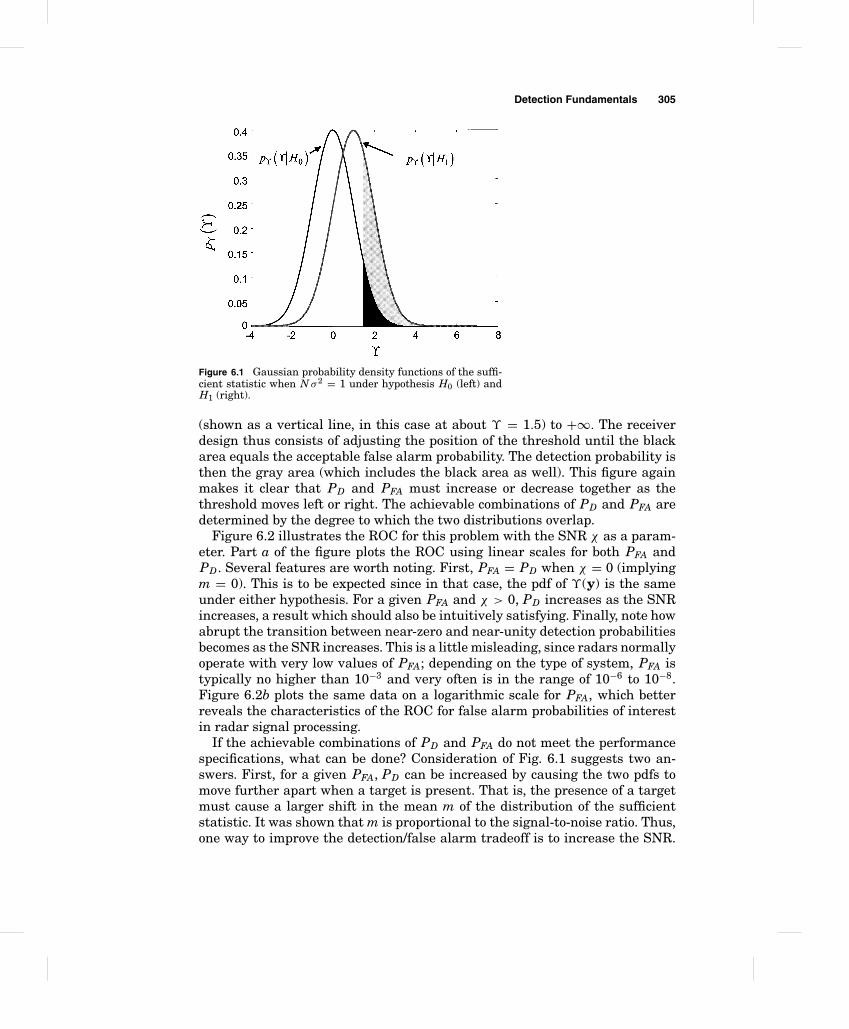
Figure 6.1 illustrates how the detection and false alarm probabilities followfrom the pdfs under the two hypotheses and the threshold, and how their rel-ative values depend on the relation between the two pdfs. Two Gaussian pdfswith variance equal to one are shown. The leftmost has a zero mean, while therightmost has a mean of 1. The left pdf is N(0, 1), while the right pdf is N(1, 1).With Nβ2 = 1 and m = 1/N , these fit the model of Example 1.3. PD and PFAare the areas under the right and left pdfs, respectively, from the threshold
Detection Fundamentals 305
Figure 6.1 Gaussian probability density functions of the suffi-cient statistic when N σ 2 = 1 under hypothesis H0 (left) andH1 (right).
(shown as a vertical line, in this case at about ϒ = 1.5) to +∞. The receiverdesign thus consists of adjusting the position of the threshold until the blackarea equals the acceptable false alarm probability. The detection probability isthen the gray area (which includes the black area as well). This figure againmakes it clear that PD and PFA must increase or decrease together as thethreshold moves left or right. The achievable combinations of PD and PFA aredetermined by the degree to which the two distributions overlap.
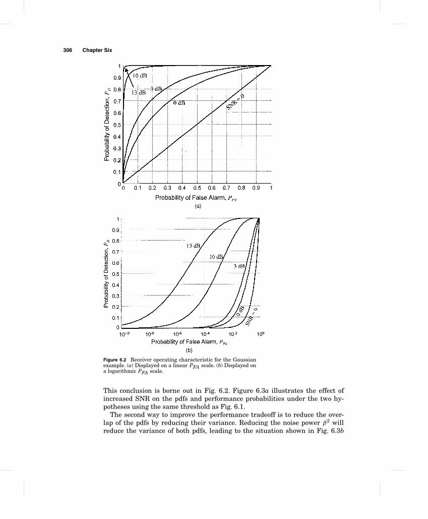
Figure 6.2 illustrates the ROC for this problem with the SNR χ as a param-eter. Part a of the figure plots the ROC using linear scales for both PFA andPD. Several features are worth noting. First, PFA = PD when χ = 0 (implyingm = 0). This is to be expected since in that case, the pdf of ϒ(y) is the sameunder either hypothesis. For a given PFA and χ > 0, PD increases as the SNRincreases, a result which should also be intuitively satisfying. Finally, note howabrupt the transition between near-zero and near-unity detection probabilitiesbecomes as the SNR increases. This is a little misleading, since radars normallyoperate with very low values of PFA; depending on the type of system, PFA istypically no higher than 10−3 and very often is in the range of 10−6 to 10−8.Figure 6.2b plots the same data on a logarithmic scale for PFA, which betterreveals the characteristics of the ROC for false alarm probabilities of interestin radar signal processing.
If the achievable combinations of PD and PFA do not meet the performancespecifications, what can be done? Consideration of Fig. 6.1 suggests two an-swers. First, for a given PFA, PD can be increased by causing the two pdfs tomove further apart when a target is present. That is, the presence of a targetmust cause a larger shift in the mean m of the distribution of the sufficientstatistic. It was shown that m is proportional to the signal-to-noise ratio. Thus,one way to improve the detection/false alarm tradeoff is to increase the SNR.
306 Chapter Six
Figure 6.2 Receiver operating characteristic for the Gaussianexample. (a) Displayed on a linear PFA scale. (b) Displayed ona logarithmic PFA scale.
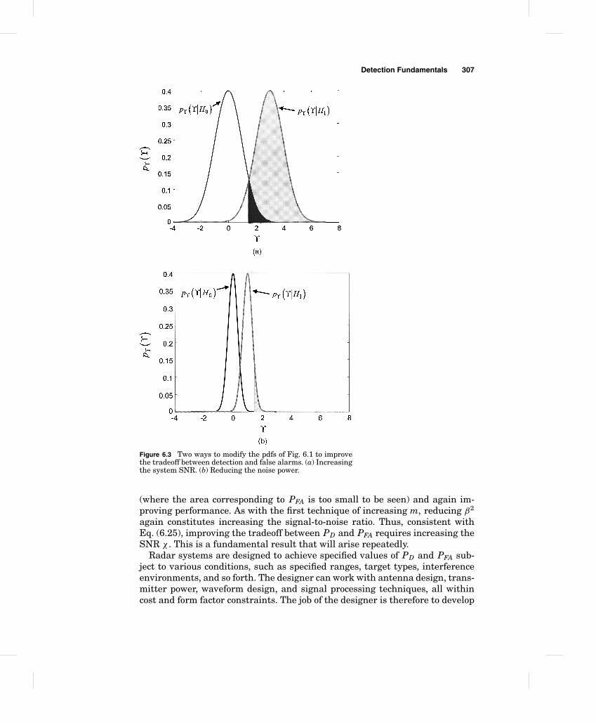
This conclusion is borne out in Fig. 6.2. Figure 6.3a illustrates the effect ofincreased SNR on the pdfs and performance probabilities under the two hy-potheses using the same threshold as Fig. 6.1.
The second way to improve the performance tradeoff is to reduce the over-lap of the pdfs by reducing their variance. Reducing the noise power β2 willreduce the variance of both pdfs, leading to the situation shown in Fig. 6.3b
Detection Fundamentals 307
Figure 6.3 Two ways to modify the pdfs of Fig. 6.1 to improvethe tradeoff between detection and false alarms. (a) Increasingthe system SNR. (b) Reducing the noise power.
(where the area corresponding to PFA is too small to be seen) and again im-proving performance. As with the first technique of increasing m, reducing β2
again constitutes increasing the signal-to-noise ratio. Thus, consistent withEq. (6.25), improving the tradeoff between PD and PFA requires increasing theSNR χ . This is a fundamental result that will arise repeatedly.
Radar systems are designed to achieve specified values of PD and PFA sub-ject to various conditions, such as specified ranges, target types, interferenceenvironments, and so forth. The designer can work with antenna design, trans-mitter power, waveform design, and signal processing techniques, all withincost and form factor constraints. The job of the designer is therefore to develop
308 Chapter Six
a radar system design which ultimately results in a pair of “target absent” and“target present” pdfs at the point of detection with a small enough overlap toallow the desired PD and PFA to be achieved. If the design does not do this, thedesigner must redesign one or more of these elements to reduce the varianceof the pdfs, shift them further apart, or both until the desired performance isobtained. Thus, a significant goal of radar system design is controlling the twopdfs analogous to those in Fig. 6.1, or equivalently, maximizing the SNR.
6.2 Threshold Detection in Coherent Systems
The Gaussian problem considered so far is useful to introduce and explain all ofthe major elements of Neyman-Pearson detection, such as the likelihood ratiotest, probabilities of detection and false alarm, receiver operating character-istics, and the major design tradeoffs that follow. Furthermore, the problemseems “radar-like”: under one hypothesis, only Gaussian noise is observed;under the other, a constant was added to the noise, which could be interpretedas the echoes from a steady target. Unfortunately, this example is not a goodmodel for any radar detection problem due to at least three major limitations.
First, coherent radar systems that produce complex-valued measurementsare of most interest. The approach, demonstrated so far only for real-valueddata, must therefore be extended to the complex case; and in doing so, thecomplex signals and interference measurements must be modeled.
Second, there are unknown parameters. The analysis so far has implicitly as-sumed that such signal parameters as the noise variance and target amplitudeare known, when in fact these are not known a priori but must be estimatedif needed. To complicate matters further, some parameters are linked. Specifi-cally in radar, the (unknown) echo amplitude varies with the (unknown) echoarrival time according to the appropriate version of the radar range equation.Thus, the LRT must be generalized to develop a technique that can work whensome signal parameters are unknown. This extension will introduce the ideaof threshold detection.
Finally, as seen in Chap. 2, there are a number of established models for radarsignal phenomenology that must be incorporated. In particular, it is necessaryto account for fluctuating targets, i.e., statistical variations in the amplitude ofthe target components of the measured data when a target is present. Further-more, while the Gaussian pdf remains a good model for noise, in many problemsthe dominant interference is clutter, which may have one of the distinctly non-Gaussian pdfs discussed in Chap. 2.
The next subsections begin addressing these shortcomings by extending theLRT to coherent systems.
6.2.1 The Gaussian case for coherent receivers
An appropriate model for noise at the output of a coherent receiver was de-veloped in Chap. 2. It was shown there that if the noise in the system prior
Detection Fundamentals 309
to quadrature signal generation is a zero mean, white Gaussian process withpower β2 = kT,† the I and Q channels will each contain independent, identicallydistributed zero-mean white Gaussian processes with power kT/2 = β2/2. Thatis, the noise power splits evenly but independently between the two channels. Acomplex noise process for which the real and imaginary parts are i.i.d. is calleda circular random process (Dudgeon and Johnson, 1993). The expression forthe joint pdf of N complex samples of the circular Gaussian random process is
py(y) = 1det{πSy} exp
{−(y − m)H S−1y (y − m)
}(6.26)
where m is the N × 1 vector mean of the N × 1 vector signal y = m + w, Sy isthe N × N covariance matrix of y
Sy = E{yyH } − mmH (6.27)
and H is the Hermitian (conjugate transpose) operator. In most cases the noisesamples are i.i.d. so that Sy = β2IN, which in turn means that det{πSy} =π N β2N . Treatment of the case where the noise samples are not equal-variance,and the colored noise case where Sy is not even diagonal, is beyond the scope ofthis text. The reader is referred to the books by Dudgeon and Johnson (1993)and Kay (1998) for these more complex situations.
Equation (6.26) now reduces to
py(y) = 1π N β2N exp
{− 1
β2 (y − m)H (y − m)}
(6.28)
Further simplifications occur when all of the means under H1 are identical sothat m = m1N, where m can now be complex-valued. In this case Eq. (6.28)reduces slightly further to
py (y) = 1π N β2N exp
{− 1
β2 (y − m1N )H (y − m1N )}
(6.29)
The LRT test for the coherent version of the previous Gaussian example canbe obtained by repeating the steps in the example of Eqs. (6.22) through (6.25)using the pdf of Eq. (6.28), with m = 0N under hypothesis H0 and m �= 0Nunder H1. The log likelihood ratio is
ln � = 1β2 {2Re[mH y] − mH m}
= 2β2 Re
{N−1∑n=0
m∗yn
}− 1
β2 N |m|2 (6.30)
†Here T refers to receiver temperature, not the detection threshold. Which meaning of T isintended should be clear from context throughout this chapter.
310 Chapter Six
where the second line of Eq. (6.30) applies only to the case where the meansare identical (m = m1N ).
Some interpretation of Eq. (6.30) is in order. The term mH y is the dot prod-uct of the complex vectors m and y. As seen in Chap. 1, this dot product rep-resents an FIR filtering operation, evaluated at the particular instant whenthe equivalent impulse response mH and the data vector y completely overlap.Furthermore, since the impulse response of the filter is identical to the signalto be detected under hypothesis H1, namely the presence of the mean m inthe data, it is a matched filter, a concept discussed in detail in previous chap-ters. Restated, the impulse response is directly related (“matched”) to the signalcomponent whose presence one seeks to detect. In this example, the “signal” isjust the vector of means, but the same reasoning applies if the elements of mare the samples of a modulated waveform or any other function of interest.
The second term in ln�, which is the complex dot product of m with itself,expands to mH m = ∑N−1
n=0 |mn|2, which is just the energy in m. Denote thisquantity as E. In the equal means case, this is just E = N |m|2.
Finally, note the Re{} operator applied to the matched filter output mH y.Because m and y are complex, one might be concerned that the dot productcould be purely imaginary or nearly so, such that Re{mH y } ≈ 0. The measureddata y would then have little or no effect on the threshold test. For this example,under hypothesis H0 m = 0N and the Re{} operator is inconsequential. Underhypothesis H1, each element of m is a complex number of the form mne j θn. Ifthe target really is present, i.e., H1 is in fact true, the elements of the measureddata vector y = m + w will be of the form mne j θn + wn, where wn is a zero meancomplex Gaussian noise sample. It then follows that
mH y = mH m + mH w
=N−1∑n=0
|mn|2 +N−1∑n=0
wn mne− j θn (6.31)
The first term is again the energy E in the signal m; this is real-valued andtherefore unaffected by the Re{} operator. The second term is simply weightedand integrated noise samples. While the phase of this noise component andtherefore the effect of the Re{} operator is random, the sum will tend to zero asmore samples are integrated.
It is evident by inspection of Eq. (6.30) that the sufficient statistic is nowRe{mH y}. Expressing the LRT in its sufficient statistic form for the complexcase
ϒ = Re{mH y}H1><H0
β2
2ln(−λ) + E
2= T (6.32)
Note that if m = m1N, the term Re{mH y} = m∑
yn and Eq. (6.32) reducesto Eq. (6.13) again. To complete consideration of the complex Gaussian case,
Detection Fundamentals 311
its performance, i.e., PD and PFA, must be determined. The sufficient statisticϒ = Re{mH y} = Re{∑m∗
n yn} is just a sum of Gaussian random variables, andso will also be Gaussian. To determine the performance of the coherent detector,the pdf of ϒ must be determined under each hypothesis. To do so it is useful tofirst consider the quantity z = mH y, which will be a complex Gaussian. Firstsuppose hypothesis H0 is true. In this case the {yn} are zero mean, and thereforeso is z. Because the {yn} are independent, the variance of z is just the sum ofthe variances of the individual weighted samples
var(z) =N−1∑n=0
var(m∗n yn)
=N−1∑n=0
|mn|2β2 = Eβ2 (6.33)
Thus, under hypothesis H0, z ∼ N(0,Eβ2). Similarly, under hypothesisH1y = m + w and z ∼ N(E,Eβ2). Note that the mean of z is real in bothcases. The power of the complex Gaussian noise splits evenly between thereal and imaginary parts of z (Kay, 1998). Since ϒ = Re{mH y}, it follows thatϒ ∼ N(0,Eβ2/2) under H0 and ϒ ∼ N(E,Eβ2/2) under H1. Following the pro-cedure used in Example 7.2, it can be seen that
PFA = 12
[1 − erf
(T√β2 E
)](6.34)
Repeating the development of Eqs. (6.22) to (6.24) gives the probability of de-tection
PD = 12
[1 − erf
{erf−1(1 − 2PFA) −
√Eβ2
}]
= 12
erfc
{erfc−1(2PFA) −
√Eβ2
}(6.35)
Note again that the last term in Eq. (6.35) is the square root of the energy inthe “signal” m, divided this time by the noise power β2, i.e., the signal-to-noiseratio. Thus Eq. (6.35) can be written as
PD = 12
[1 − erf {erf−1(1 − 2PFA) − √χ}]
= 12
erfc {erfc−1(2PFA) − √χ} (6.36)
Finally, in the equal means case when m = m1N , Eq. (6.35) is similar (but notidentical) to Eq. (6.24). The coherent case includes the term
√Nm2/β2 instead
of√
Nm2/2β2 because all of the signal energy competes with only half of thenoise power.
312 Chapter Six
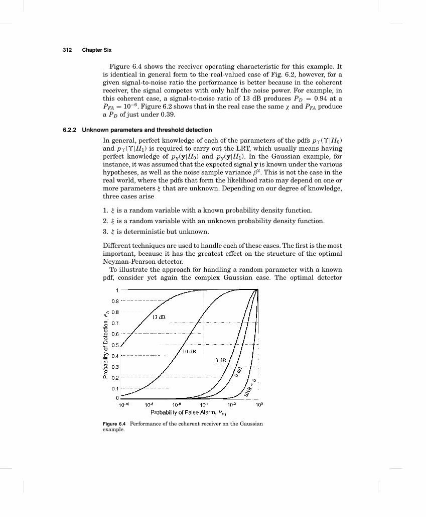
Figure 6.4 shows the receiver operating characteristic for this example. Itis identical in general form to the real-valued case of Fig. 6.2, however, for agiven signal-to-noise ratio the performance is better because in the coherentreceiver, the signal competes with only half the noise power. For example, inthis coherent case, a signal-to-noise ratio of 13 dB produces PD = 0.94 at aPFA = 10−6. Figure 6.2 shows that in the real case the same χ and PFA producea PD of just under 0.39.
6.2.2 Unknown parameters and threshold detection
In general, perfect knowledge of each of the parameters of the pdfs pϒ (ϒ |H0)and pϒ (ϒ |H1) is required to carry out the LRT, which usually means havingperfect knowledge of py(y|H0) and py(y|H1). In the Gaussian example, forinstance, it was assumed that the expected signal y is known under the varioushypotheses, as well as the noise sample variance β2. This is not the case in thereal world, where the pdfs that form the likelihood ratio may depend on one ormore parameters ξ that are unknown. Depending on our degree of knowledge,three cases arise
1. ξ is a random variable with a known probability density function.
2. ξ is a random variable with an unknown probability density function.
3. ξ is deterministic but unknown.
Different techniques are used to handle each of these cases. The first is the mostimportant, because it has the greatest effect on the structure of the optimalNeyman-Pearson detector.
To illustrate the approach for handling a random parameter with a knownpdf, consider yet again the complex Gaussian case. The optimal detector
Figure 6.4 Performance of the coherent receiver on the Gaussianexample.
Detection Fundamentals 313
implemented a matched filter operation mH y, followed by the Re{} operator.The success of the matched filter structure depended on knowing exactly theconstant component of y = m + w under hypothesis H1, so that the filtercoefficients could be set equal to m and the filter output would be real-valued.Recall that, when applied to radar, y under H0 is considered to consist only ofsamples w of receiver noise, and under H1 to consist of noisy samples m + w ofthe echoes from a radar target over multiple pulses, or alternately successivefast-time samples of the waveform of one pulse echo from a target.
Claiming perfect knowledge of m implies knowing the range to the target veryprecisely, since a variation in one-way range of only λ/4 causes the received echophase to completely reverse, i.e., to change by 180˚. At microwave frequencies,this is typically only 15 to 30 cm (at L band to UHF) to a fraction of a centimeter(at millimeter wave frequencies). Because this precision is usually unrealistic, itis more reasonable to assume m is known only to within a phase factor exp( jθ ),where the phase angle θ is considered to be a random variable distributeduniformly over (0, 2 π ] and independent of the random variables {mn}. In otherwords, m = m exp( jθ ), where m is known exactly but θ is a random phase.(Note that the energy in m is the same as that in m, that is, mH m = mH m.)This “unknown phase” assumption cannot usually be avoided in radar. What isits effect on the optimal detector and its performance?
The goal remains to carry out the LRT, so it is necessary to return to its basicdefinition of Eq. (6.6) and determine py(y|H0) and py(y|H1), both of whichnow presumably depend on θ ,† and use the technique known as the Bayesianapproach for random parameters with known pdfs (Kay, 1998). Specifically,compute the pdf under Hi by separately averaging the conditional pdfs py(y|Hi)over θ
py(y|Hi) =∫
py(y|Hi, θ ) pθ (θ ) dθ i = 0, 1 (6.37)
The unconditional pdfs py(y|Hi) are then used to define the likelihood ratio inthe usual way.
As an example of the Bayesian approach for random parameters, consideragain the complex Gaussian case, but now with an unknown phase in the data,m = m exp( jθ ). The conditional pdf of the observations y becomes, under eachof the two hypotheses,
py(y|H0, θ ) = 1π N β2N exp
[− 1
β2 yH y]
(6.38)
py(y|H1, θ ) = 1π N β2N exp
[− 1
β2 (y − me j θ )H (y − me j θ )]
†An alternative approach called the generalized likelihood ratio test (GLRT), in which the un-known parameter(s) are replaced by their maximum likelihood estimates, is discussed in manydetection theory texts (e.g., Kay, 1998).
314 Chapter Six
Expanding the exponent in Eq. (6.38) gives
py(y|H1, θ ) = 1π N β2N exp
[− 1
β2 (yH y − 2Re {mH ye j θ } + E)]
= 1π N β2N exp
[− 1
β2 (yH y − 2|mH y| cos θ + E)]
(6.39)
Notice that py(y|H0) does not depend on θ after all (not surprising sincethere is no target present in this case to present an unknown phase), so it isnot necessary to apply Eq. (6.37). However, in py(y|H1) the dependence on θ isexplicit. Assuming a uniform random phase and applying Eq. (6.37) under H1gives, after minor rearrangement
py(y|H1) = 1π N β2N e−(yH y+E)/β2 1
2π
∫ 2π
0exp[
2β2 |mH y| cos θ
]dθ (6.40)
Equation (6.40) is a standard integral. Specifically, integral 9.6.16 in the bookby Abramowitz and Stegun (1972) is
1π
∫ π
0e±z cos θdθ = I0(z) (6.41)
where I0(z) is the modified Bessel function of the first kind. Using this resultand properties of the cosine function, Eq. (6.40) becomes
py(y|H1) = 1π N β2N e−(yH y+E)/β2
I0
(2|mH y|
β2
)(6.42)
The log-LRT now becomes
ln � = ln[
I0
(2|mH y|
β2
)]− E
β2
H1><H0
ln(−λ) (6.43)
or, in sufficient statistic form
ϒ = ln[
I0
(2|mH y|
β2
)] H1><H0
ln(−λ) + Eβ2 = T (6.44)
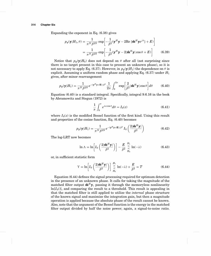
Equation (6.44) defines the signal processing required for optimum detectionin the presence of an unknown phase. It calls for taking the magnitude of thematched filter output mH y, passing it through the memoryless nonlinearityln[I0()], and comparing the result to a threshold. This result is appealing inthat the matched filter is still applied to utilize the internal phase structureof the known signal and maximize the integration gain, but then a magnitudeoperation is applied because the absolute phase of the result cannot be known.Also, note that the argument of the Bessel function is the energy in the matchedfilter output divided by half the noise power; again, a signal-to-noise ratio.
Detection Fundamentals 315
Only half of the noise power appears because the total noise power in the com-plex case is split between the real and imaginary channels.
As a practical matter, it is desirable to avoid having to compute the naturallogarithm and Bessel function for every threshold test, since these might occurmillions of times per second in some systems. Because the function ln[I0()] ismonotonically increasing, the same detection results can be obtained by simplycomparing its argument 2|mH y|/β2 to a modified threshold. Equation (6.44)then becomes simply
|mH y|H1><H0
T ′ (6.45)
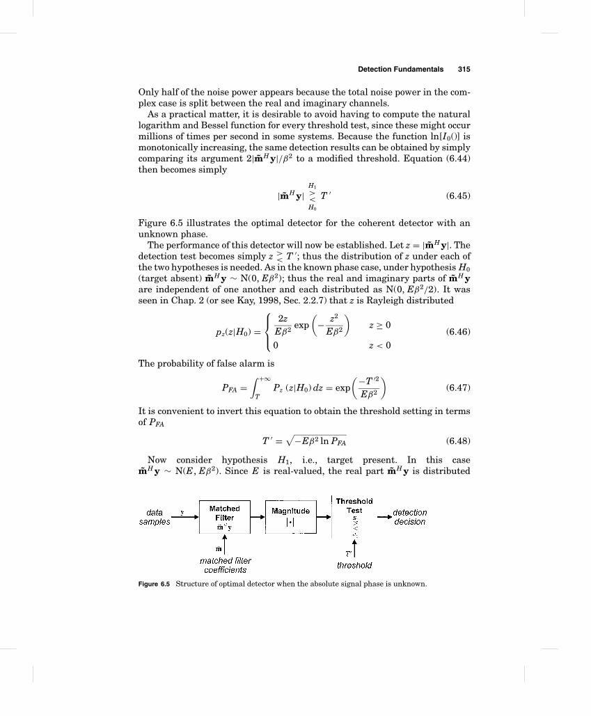
Figure 6.5 illustrates the optimal detector for the coherent detector with anunknown phase.
The performance of this detector will now be established. Let z = |mH y|. Thedetection test becomes simply z >
< T ′; thus the distribution of z under each ofthe two hypotheses is needed. As in the known phase case, under hypothesis H0(target absent) mH y ∼ N(0, Eβ2); thus the real and imaginary parts of mH yare independent of one another and each distributed as N(0, Eβ2/2). It wasseen in Chap. 2 (or see Kay, 1998, Sec. 2.2.7) that z is Rayleigh distributed
pz(z|H0) =
2zEβ2 exp
(− z2
Eβ2
)z ≥ 0
0 z < 0(6.46)
The probability of false alarm is
PFA =∫ +∞
TPz (z|H0) dz = exp
(−T ′2
Eβ2
)(6.47)
It is convenient to invert this equation to obtain the threshold setting in termsof PFA
T ′ =√
−Eβ2 ln PFA (6.48)
Now consider hypothesis H1, i.e., target present. In this casemH y ∼ N(E, Eβ2). Since E is real-valued, the real part mH y is distributed
Figure 6.5 Structure of optimal detector when the absolute signal phase is unknown.
316 Chapter Six
as N(E, Eβ2/2) while the imaginary part is distributed as N(0, Eβ2/2). It againfollows from Chap. 2 (or see Kay, 1998, Sec. 2.2.6 or Papoulis, 1984) that thepdf of z is
pz(z|H1) =
2zEβ2 exp
[− 1
Eβ2 (z2 + E2)]
I0
(2 zβ2
)z ≥ 0
0 z < 0(6.49)
where I0(z) is again the modified Bessel function of the first kind. Equation (6.49)is the Rician pdf. The probability of detection is obtained by integrating it fromT ′ to +∞.
In normalized form, the required integral is
QM(α, γ ) =∫ +∞
γ
t exp[−1
2(t2 + α2)
]I0(αt) dt (6.50)
The expression QM(α, γ ) is known as Marcum’s Q function. It arises frequentlyin radar detection calculations. A closed form for this integral is not known.Algorithms for evaluating QM(α, γ ) are compared by Cantrell and Ojha (1987).The “Communications Toolbox” optional package of MATLAB™ includes amarcumq function; another MATLAB™ algorithm is given by Kay (1998).
By defining a change of variables, the integral of Eq. (6.49) can be put intothe form of Eq. (6.50). Specifically, choose t = z/
√Eβ2/2 and α = √
2E/β.Substituting into Eq. (6.49) and doing the integration gives
PD = QM
√
2Eβ2 ,
√2T ′2
Eβ2
(6.51)
Finally, noting that E/β2 is the signal-to-noise ratio χ and expressing thethreshold in terms of the false alarm probability using Eq. (6.48) gives
PD = QM
(√2χ ,√
−2 ln PFA
)(6.52)
It is usually the case that the energy E in m or m is not known. Fortunately,Eq. (6.52) does not depend on E (or the noise power β2) explicitly, but only ontheir ratio χ , so that it is possible to generate the ROC without this information.However, actually implementing the detector requires a specific value of thethreshold T ′ as given in Eq. (6.48), and this does require knowledge of both Eand β2. One way to avoid this problem is to replace the matched filter coefficientsm with a normalized coefficient vector m = m/Em, where Em is the energy inm. This choice simply normalizes the gain of the matched filter to 1. The energyin this modified sequence is E = 1, leading to a modified threshold
T =√
−β2 ln PFA (6.53)
The reduced matched filter gain, along with the reduced threshold, results inno change to the ROC, so that Eq. (6.52) remains valid. Setting of the threshold
Detection Fundamentals 317
T still requires knowledge of the noise power β2; removal of this restrictionis the subject of Chap. 7. The handling of unknown amplitude parameters isdiscussed in somewhat more detail in Sec. 6.2.4.
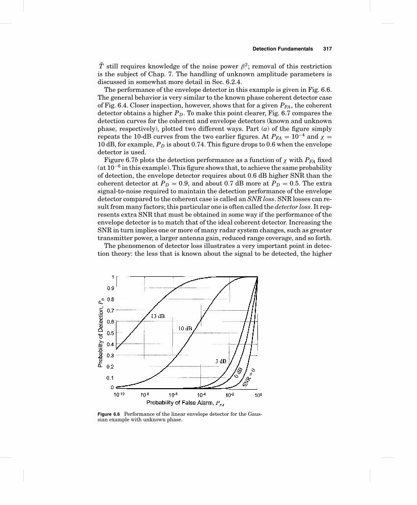
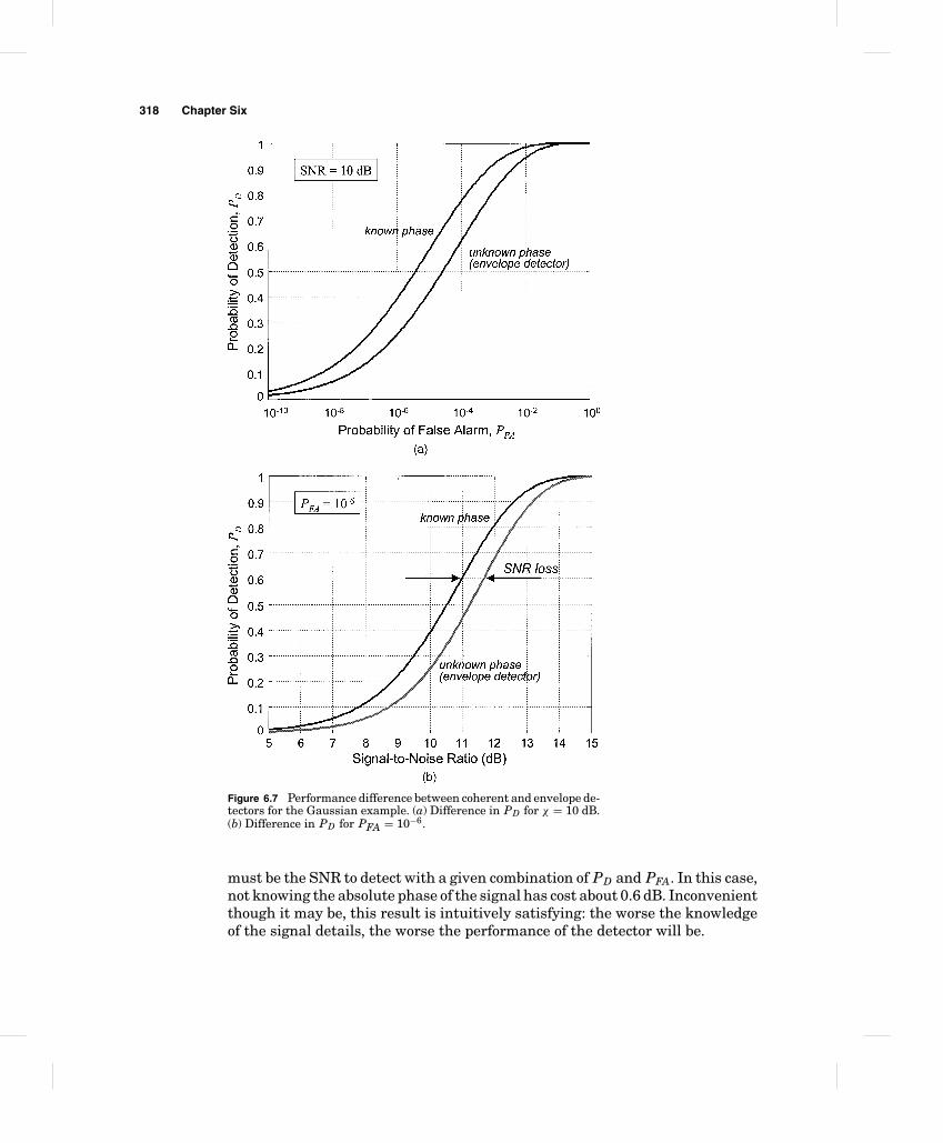
The performance of the envelope detector in this example is given in Fig. 6.6.The general behavior is very similar to the known phase coherent detector caseof Fig. 6.4. Closer inspection, however, shows that for a given PFA, the coherentdetector obtains a higher PD. To make this point clearer, Fig. 6.7 compares thedetection curves for the coherent and envelope detectors (known and unknownphase, respectively), plotted two different ways. Part (a) of the figure simplyrepeats the 10-dB curves from the two earlier figures. At PFA = 10−4 and χ =10 dB, for example, PD is about 0.74. This figure drops to 0.6 when the envelopedetector is used.
Figure 6.7b plots the detection performance as a function of χ with PFA fixed(at 10−6 in this example). This figure shows that, to achieve the same probabilityof detection, the envelope detector requires about 0.6 dB higher SNR than thecoherent detector at PD = 0.9, and about 0.7 dB more at PD = 0.5. The extrasignal-to-noise required to maintain the detection performance of the envelopedetector compared to the coherent case is called an SNR loss. SNR losses can re-sult from many factors; this particular one is often called the detector loss. It rep-resents extra SNR that must be obtained in some way if the performance of theenvelope detector is to match that of the ideal coherent detector. Increasing theSNR in turn implies one or more of many radar system changes, such as greatertransmitter power, a larger antenna gain, reduced range coverage, and so forth.
The phenomenon of detector loss illustrates a very important point in detec-tion theory: the less that is known about the signal to be detected, the higher
Figure 6.6 Performance of the linear envelope detector for the Gaus-sian example with unknown phase.
318 Chapter Six
Figure 6.7 Performance difference between coherent and envelope de-tectors for the Gaussian example. (a) Difference in PD for χ = 10 dB.(b) Difference in PD for PFA = 10−6.
must be the SNR to detect with a given combination of PD and PFA. In this case,not knowing the absolute phase of the signal has cost about 0.6 dB. Inconvenientthough it may be, this result is intuitively satisfying: the worse the knowledgeof the signal details, the worse the performance of the detector will be.
Detection Fundamentals 319
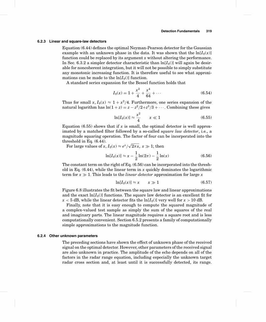
6.2.3 Linear and square-law detectors
Equation (6.44) defines the optimal Neyman-Pearson detector for the Gaussianexample with an unknown phase in the data. It was shown that the ln[I0(x)]function could be replaced by its argument x without altering the performance.In Sec. 6.3.2 a simpler detector characteristic than ln[I0()] will again be desir-able for noncoherent integration, but it will not be possible to simply substituteany monotonic increasing function. It is therefore useful to see what approxi-mations can be made to the ln[I0()] function.
A standard series expansion for the Bessel function holds that
I0(x) = 1 + x2
4+ x4
64+ · · · (6.54)
Thus for small x, I0(x) ≈ 1 + x2/4. Furthermore, one series expansion of thenatural logarithm has ln(1 + z) = z − z2/2+z3/3 + · · · . Combining these gives
ln[I0(x)] ≈ x2
4x � 1 (6.55)
Equation (6.55) shows that if x is small, the optimal detector is well approx-imated by a matched filter followed by a so-called square law detector, i.e., amagnitude squaring operation. The factor of four can be incorporated into thethreshold in Eq. (6.44).
For large values of x, I0(x) ≈ ex/√
2πx, x � 1; then
ln[I0(x)] ≈ x − 12
ln(2π ) − 12
ln(x) (6.56)
The constant term on the right of Eq. (6.56) can be incorporated into the thresh-old in Eq. (6.44), while the linear term in x quickly dominates the logarithmicterm for x � 1. This leads to the linear detector approximation for large x
ln[I0(x)] ≈ x x � 1 (6.57)
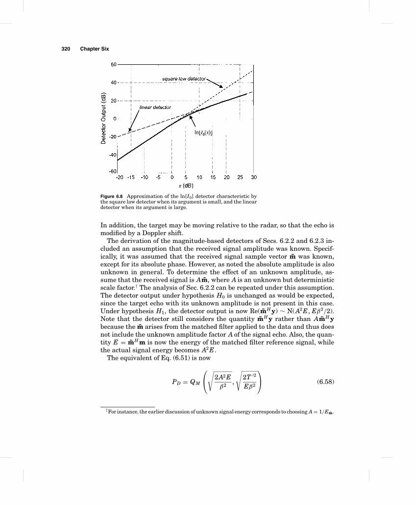
Figure 6.8 illustrates the fit between the square law and linear approximationsand the exact ln[I0()] functions. The square law detector is an excellent fit forx < 5 dB, while the linear detector fits the ln[I0()] very well for x > 10 dB.
Finally, note that it is easy enough to compute the squared magnitude ofa complex-valued test sample as simply the sum of the squares of the realand imaginary parts. The linear magnitude requires a square root and is lesscomputationally convenient. Section 6.5.2 presents a family of computationallysimple approximations to the magnitude function.
6.2.4 Other unknown parameters
The preceding sections have shown the effect of unknown phase of the receivedsignal on the optimal detector. However, other parameters of the received signalare also unknown in practice. The amplitude of the echo depends on all of thefactors in the radar range equation, including especially the unknown targetradar cross section and, at least until it is successfully detected, its range.
320 Chapter Six
Figure 6.8 Approximation of the ln[I0] detector characteristic bythe square law detector when its argument is small, and the lineardetector when its argument is large.
In addition, the target may be moving relative to the radar, so that the echo ismodified by a Doppler shift.
The derivation of the magnitude-based detectors of Secs. 6.2.2 and 6.2.3 in-cluded an assumption that the received signal amplitude was known. Specif-ically, it was assumed that the received signal sample vector m was known,except for its absolute phase. However, as noted the absolute amplitude is alsounknown in general. To determine the effect of an unknown amplitude, as-sume that the received signal is Am, where A is an unknown but deterministicscale factor.† The analysis of Sec. 6.2.2 can be repeated under this assumption.The detector output under hypothesis H0 is unchanged as would be expected,since the target echo with its unknown amplitude is not present in this case.Under hypothesis H1, the detector output is now Re(mH y) ∼ N( A2 E, Eβ2/2).Note that the detector still considers the quantity mH y rather than AmH ybecause the m arises from the matched filter applied to the data and thus doesnot include the unknown amplitude factor A of the signal echo. Also, the quan-tity E = mH m is now the energy of the matched filter reference signal, whilethe actual signal energy becomes A2 E.
The equivalent of Eq. (6.51) is now
PD = QM
√
2A2 Eβ2 ,
√2T ′2
Eβ2
(6.58)
†For instance, the earlier discussion of unknown signal energy corresponds to choosing A = 1/Em.
Detection Fundamentals 321
As before, the second argument of Eq. (6.58) can be written in terms of theprobability of false alarm. Furthermore, because the actual signal energy isnow A2 E, the first argument is still
√2χ . Thus, the detection performance is
still given by Eq. (6.52). The unknown echo amplitude neither requires anychange in the detector structure, nor changes its performance.
Despite the unknown amplitude, the sufficient statistic was not changed.Furthermore, the probability of false alarm could be computed without knowl-edge of the amplitude. When both these conditions hold, the detection test iscalled a uniformly most powerful (UMP) test (Dudgeon and Johnson, 1993).
A UMP does not exist for the case where the signal delay (range) is unknown,which again is the only realistic assumption that can be made in radar. It istherefore necessary to resort to a generalized likelihood ration test (GLRT),in which the likelihood ratio is written as a function of the unknown signaldelay �, and then the value of � that maximizes the likelihood ratio is found.Details are given by Dudgeon and Johnson (1993). The result simply requiresevaluation of the matched filter over a range of delays. In practice, the matchedfilter is applied to the entire fast time signal; the filter output samples aresimply the matched filter response for each corresponding possible target range.The maximum output is selected and compared to the threshold. If the thresholdis crossed, a detection is declared. Furthermore, the value of � at which themaximum occurs is taken as an estimate of the target delay.
If the target is moving, an unknown Doppler shift will be imposed on theincident signal. The received echo will then be proportional not to m, but toa modified signal m′ where the samples of the reference signal m have beenmultiplied by the complex exponential sequence exp(jωDn), where ωD is thenormalized Doppler shift. The required matched filter impulse response is nowm′; if m is replaced by m′ in the derivations of Sec. 6.2.2, the same performanceresults as before will be obtained. Because ωD is unknown, however, it is nec-essary to test for different possible Doppler shifts by conducting the detectiontest for multiple possible values of ωD, similar to the procedure used to test forunknown range. If a set of K potential Doppler frequencies uniformly spacedfrom −PRF/2 to +PRF/2 is to be tested, the matched filter can be implementedfor all K frequencies at once using the pulse Doppler processing techniques de-scribed in Chap. 5.
6.3 Threshold Detection of Radar Signals
The results of the preceding sections can now be applied to some reasonablyrealistic scenarios for detecting radar targets in noise. These scenarios willalmost always include unknown parameters of the signal to be detected (thetarget), specifically, its amplitude, absolute phase, time of arrival, and Dopplershift. Detection on both a single sample of the target signal, and when multiplesamples are available, is of interest. In the latter case, as discussed in Chap. 2,the target signal is often modeled as a random process, rather than a simpleconstant; the discussion in this chapter will be limited to the four Swerling
322 Chapter Six
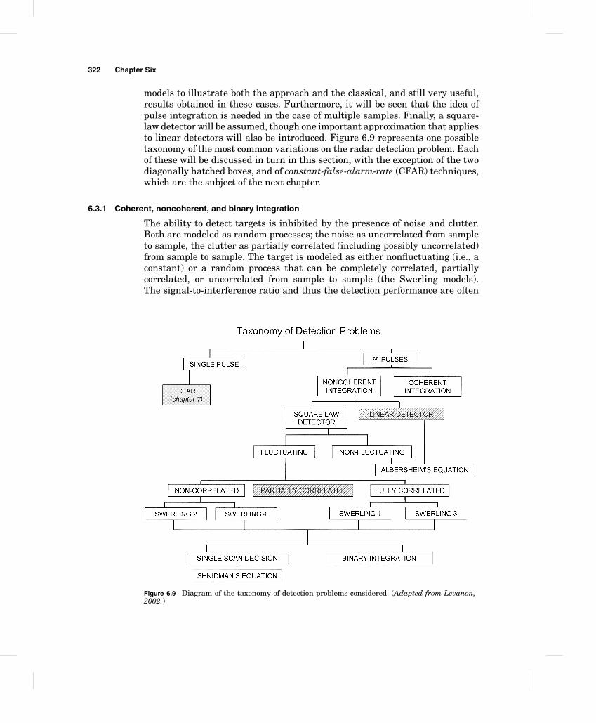
models to illustrate both the approach and the classical, and still very useful,results obtained in these cases. Furthermore, it will be seen that the idea ofpulse integration is needed in the case of multiple samples. Finally, a square-law detector will be assumed, though one important approximation that appliesto linear detectors will also be introduced. Figure 6.9 represents one possibletaxonomy of the most common variations on the radar detection problem. Eachof these will be discussed in turn in this section, with the exception of the twodiagonally hatched boxes, and of constant-false-alarm-rate (CFAR) techniques,which are the subject of the next chapter.
6.3.1 Coherent, noncoherent, and binary integration
The ability to detect targets is inhibited by the presence of noise and clutter.Both are modeled as random processes; the noise as uncorrelated from sampleto sample, the clutter as partially correlated (including possibly uncorrelated)from sample to sample. The target is modeled as either nonfluctuating (i.e., aconstant) or a random process that can be completely correlated, partiallycorrelated, or uncorrelated from sample to sample (the Swerling models).The signal-to-interference ratio and thus the detection performance are often
Figure 6.9 Diagram of the taxonomy of detection problems considered. (Adapted from Levanon,2002.)
Detection Fundamentals 323
improved by integrating (adding) multiple samples of the target and interfer-ence, motivated by the idea that the interference can be “averaged out” byadding multiple samples. This idea was first discussed in Chap. 1. Thus, ingeneral detection will be based on N samples of the target+interference. Notethat care must be taken to integrate samples that represent the same rangeand Doppler resolution cells.
Integration may be applied to the data at three different stages in the pro-cessing chain
1. After coherent demodulation, to the baseband complex-valued (I and Q, ormagnitude and phase) data. Combining complex data samples is referred toas coherent integration.
2. After envelope detection, to the magnitude (or squared or log magnitude)data. Combining magnitude samples after the phase information is dis-carded is referred to as noncoherent integration.
3. After threshold detection, to the target present/target absent decisions. Thistechnique is called binary integration.
A system could elect to use none, one, or any combination of these techniques.Many systems use at least one integration technique, and a combination ofeither coherent or noncoherent with postdetection binary integration is alsocommon. The major cost of integration is the time and energy required to ob-tain multiple samples of the same range, Doppler, and/or angle cell (or multiplethreshold detection decisions for that cell); this is time that cannot be spentsearching for targets elsewhere, or tracking already-known targets, or imag-ing other regions of interest. Integration also increases the signal processingcomputational load. Modern systems vary as to whether this is an issue: therequired operations are simple, but must be performed at a very high rate inmany systems.
In coherent integration, complex (magnitude and phase) data samples yn arecombined to form a new complex variable y
y =N−1∑n=0
yn (6.59)
As shown in Chap. 1, if the SNR of a single sample yn is χ1, the integrateddata sample y has an SNR that is N times that of the single sample yn, i.e.,χN = N χ1. That is, coherent integration attains an integration gain of N.Detection calculations are then based on the result for a single sample oftarget+noise having the improved SNR equal to χN . Thus, no special results areneeded to analyze the case of coherent integration; one simply uses the single-sample detection results for the target and interference models of interest withthe coherently integrated SNR χN .
In noncoherent integration, phase information is discarded. Instead, themagnitude or squared magnitude of the data samples is integrated. (Some-times another function of the magnitude, such as the log-magnitude, is used.)
324 Chapter Six
Most classical detection results have been developed for the square law detector,which bases detection on the quantity
z =N−1∑n=0
|yn|2 (6.60)
Consideration will be largely restricted to the square law detector in thissection.
When coherent integration is used, detection results are obtained by usingsingle-sample (N = 1) results with χ1 replaced by the integrated χN . The situ-ation for noncoherent integration is more complicated, and it will be necessaryto determine the actual probability density function of the integrated variate zto compute detection results; this is done in the next subsection.
Binary integration takes place after an initial detection decision has takenplace. That initial decision may be based on a single sample, or on data thathave already been coherently and/or noncoherently integrated. Whatever theprocessing before the threshold detection, after it the result is a choice betweenhypothesis H0, “target absent,” and H1, “target present.” Because there areonly two possible outputs of the detector each time a threshold test is made,the output is said to be binary. Multiple binary decisions can be combined in an“M out of N ” decision logic in an attempt to further improve the performance.This type of integration is discussed in Sec. 6.4.
6.3.2 Nonfluctuating targets
Now consider detection based on noncoherent integration of N samples of anonfluctuating target (sometimes called the “Swerling 0” or “Swerling 5” case)in white Gaussian noise. The amplitude and absolute phase of the target compo-nent are unknown. Thus, an individual data sample yn is the sum of a complexconstant m = m exp( jθ ) for some real amplitude m and phase θ , and a whiteGaussian noise sample wn of power β2/2 in each of the I and Q channels (totalnoise power β2)
yn = m + wn (6.61)
Under hypothesis H0, the target is absent and yn = wn. The pdf of zn = |yn| isRayleigh
pzn(zn|H0) =
2zn
β2 e−z2n/β2
zn ≥ 0
0 zn < 0(6.62)
Under hypothesis H1, zn is a Rician voltage density
pzn(zn|H1) =
2zn
β2 e−(z2n+m2)/β2
I0
(2mzn
β2
)zn ≥ 0
0 zn < 0(6.63)
Detection Fundamentals 325
Thus for a vector z of N such samples (not to be confused with the scalar sumz of samples), the joint pdfs are, for each zn ≥ 0
pz(z|H0) =N−1∏n=0
2zn
β2 e−z2n/β2
(6.64)
pz(z|H1) =N−1∏n=0
2zn
β2 e−(z2n+m2)/β2
I0
(2mzn
β2
)(6.65)
The LRT and log-LRT become
� =N−1∏n=0
e−m2/β2I0
(2mzn
β2
)= e−m2/β2
N−1∏n=0
I0
(2mzn
β2
) H1><H0
− λ (6.66)
ln � = −m2
β2 +N−1∑n=0
ln[
I0
(2mzn
β2
)] H1><H0
ln(−λ) (6.67)
Incorporating the term involving the ratio of signal power and noise power onthe left hand side into the threshold gives
N−1∑n=0
ln[
I0
(2mzn
β2
)] H1><H0
ln(−λ) + m2
β2 = T (6.68)
Equation (6.68) shows that, given N noncoherent samples of a nonfluctuatingtarget in white noise, the optimal Neyman-Pearson detection test scales eachsample by the quantity 2m/β2, passes it through the monotonic nonlinearityln[I0()], and then integrates the processed samples and performs a thresholdtest. There are two practical problems with this equation. First, as noted earlier,it is desirable to avoid computing the function ln[I0()] possibly millions of timesper second. Second, both the target amplitude m and the noise power β2 mustbe known to perform the required scaling. The test can be simplified by usingthe results of Sec. 6.2.3. Applying the square law detector approximation ofEq. (6.55) to Eq. (6.68) gives the test
N−1∑n=0
m2z2n
β4
H1><H0
T (6.69)
Combining all constants into the threshold gives us the final noncoherent inte-gration detection rule
z =N−1∑n=0
z2n
H1><H0
β4Tm2 = T ′ (6.70)
326 Chapter Six
Equation (6.70) states that the squared magnitudes of the data samples aresimply integrated and the integrated sum compared to a threshold to decidewhether a target is present or not. Note that the integrated variate z is thesufficient statistic ϒ for this problem.
The performance of the detector given in Eq. (6.70) must now be determined.It is convenient to scale the zn, replacing them with the new variables z′
n = zn/β
and thus replacing z with z′ = ∑ (z′n)2 = z2/β2; such a scaling does not change
the performance, but merely alters the threshold value that corresponds to aparticular PD or PFA. The pdf of z′
n is still either Rayleigh or Rician voltage asin Eqs. (6.62) and (6.63), but now with unit noise variance
pz′n(z′
n|H0) ={
2z′ne−z′2
n z′n ≥ 0
0 z′n < 0
(6.71)
pz′n(z′
n|H1) ={
2z′ne−(
z′2n+χ)
I0(2z′n√
χ ) z′n ≥ 0
0 z′n < 0
(6.72)
where χ = m2/β2 is the signal-to-noise ratio. Since a square law detector isbeing used, the pdf of rn = (z′
n)2 is needed (thus z′ = ∑ rn); this is exponentialunder H0 and a Rician power density under H1
prn(rn|H0) ={
e−rn rn ≥ 00 rn < 0
(6.73)
prn(rn|H1) ={
e−(rn+χ ) I0(2√
χrn) rn ≥ 00 rn < 0
(6.74)
Since z′ is the sum of N scaled random variables rn = (z′n)2, the pdf of z′ is the
N-fold convolution of the pdf given in Eq. (6.73) or (6.74) (Papoulis, 1984). Thisis most easily found using characteristic functions (CFs). The characteristicfunction C(q) corresponding to a pdf p(z) is given by (Papoulis, 1984)
Cz(q) =∫ +∞
−∞pz(z) e jqz dz (6.75)
Note that Cz(q) is just the Fourier transform of pz(z), though with the sign of thecomplex exponential kernel chosen opposite from the definition commonly usedin electrical engineering texts. It still follows, however, that the characteristicfunction of the N-fold convolution of the pdfs is the product of their individualcharacteristic functions.
Under hypothesis H0 the CF of rn can be readily shown from Eqs. (6.73) and(6.75) to be
Crn(q) = 11 − j q
(6.76)
Detection Fundamentals 327
The characteristic function of z′ is therefore
Cz′ (q) = [Cr (q)]N =(
11 − jq
)N
(6.77)
The pdf of z′ is obtained by inverting its characteristic function using the inverseFourier transform
pz′ (z′|H0) = 12π
∫ ∞
−∞Cz′ (q)e−jqz′
dq (6.78)
Using Eq. (6.77) in Eq. (6.78) and referring to any good Fourier transform table(with allowance for the reversed sign of the Fourier kernel in the definition ofthe characteristic function), the Erlang density (a special case of the gammadensity) is obtained (Papoulis, 1984)
p′z(z
′|H0) =
(z′)N−1
(N −1)!e−z′
z′ ≥ 0
0 z′ < 0(6.79)
Note that this reduces to the exponential pdf when N = 1, as would be expectedsince in that case z′ is the magnitude squared of a single sample of complexGaussian noise.
The probability of false alarm is obtained by integrating Eq. (6.79) from thethreshold value to +∞. The result is (Abramowitz and Stegun, 1972)
PFA =∫ ∞
T
(z′)N−1
(N −1)!e−z′
dz′ = 1 − I(
T√N
, N − 1)
(6.80)
where I (u, M) =∫ u
√M+1
0
e−τ τ M
M!dτ (6.81)
is Pearson’s form of the incomplete gamma function. For a single sample(N = 1), Eq. (6.80) reduces to the especially simple result
PFA = e−T (6.82)
so that T = − ln PFA.Equation (6.80) can be used to determine the probability of false alarm PFA
for a given threshold T or, more likely, to determine the required value of Tfor a desired PFA. Now the probability of detection PD corresponding to thesame threshold must be determined. Start by finding the pdf of the normal-ized, integrated, and square-law-detected samples under hypothesis H1. Eachindividual data sample rn is Rician (Eq. (6.74)); the corresponding characteristicfunction is
Crn(q) = 1q + 1
e−χ [q/(q+1)] (6.83)
328 Chapter Six
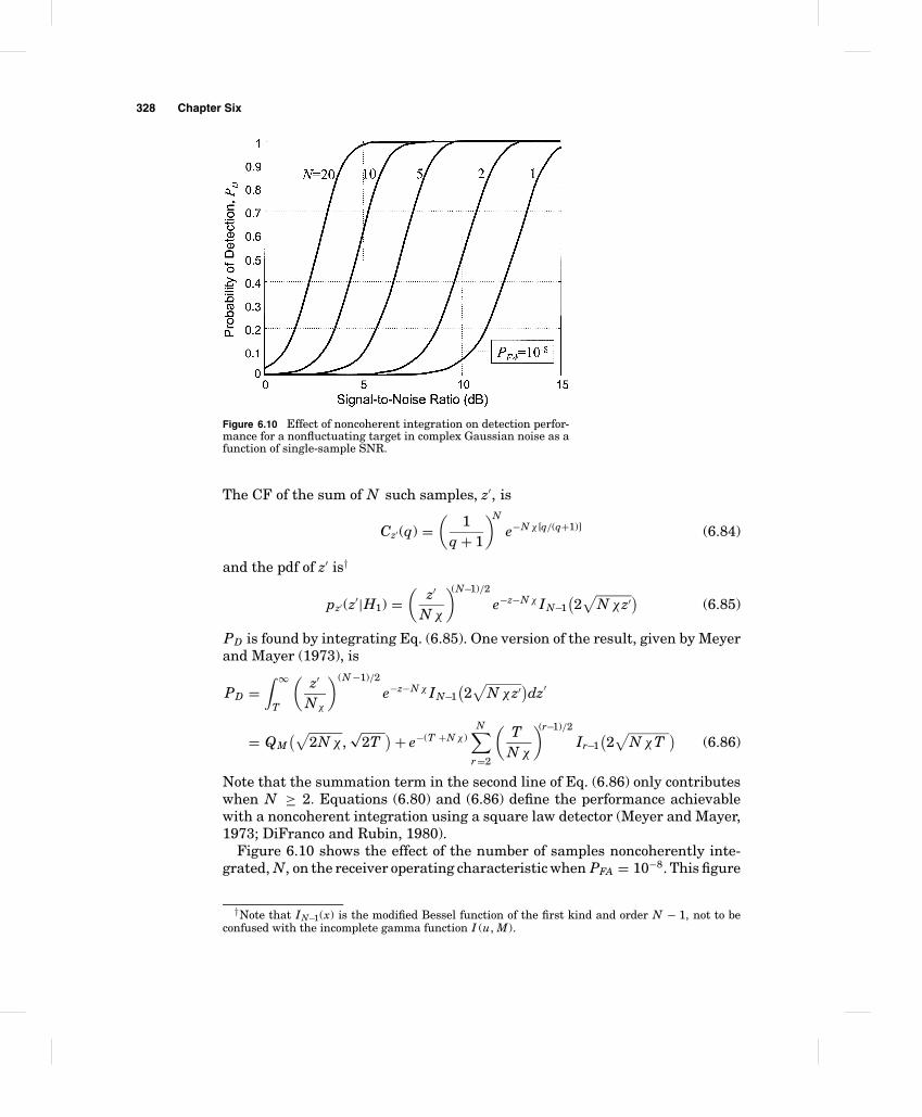
Figure 6.10 Effect of noncoherent integration on detection perfor-mance for a nonfluctuating target in complex Gaussian noise as afunction of single-sample SNR.
The CF of the sum of N such samples, z′, is
Cz′ (q) =(
1q + 1
)N
e−N χ [q/(q+1)] (6.84)
and the pdf of z′ is†
pz′ (z′|H1) =(
z′
N χ
)(N−1)/2
e−z−N χ IN−1(2√
N χz′) (6.85)
PD is found by integrating Eq. (6.85). One version of the result, given by Meyerand Mayer (1973), is
PD =∫ ∞
T
(z′
Nχ
)(N −1)/2
e−z−N χ IN−1(2√
N χz′)dz′
= QM(√
2N χ ,√
2T)+ e−(T +N χ )
N∑r =2
(T
N χ
)(r−1)/2
Ir−1(2√
N χT)
(6.86)
Note that the summation term in the second line of Eq. (6.86) only contributeswhen N ≥ 2. Equations (6.80) and (6.86) define the performance achievablewith a noncoherent integration using a square law detector (Meyer and Mayer,1973; DiFranco and Rubin, 1980).
Figure 6.10 shows the effect of the number of samples noncoherently inte-grated, N, on the receiver operating characteristic when PFA = 10−8. This figure
†Note that IN−1(x) is the modified Bessel function of the first kind and order N − 1, not to beconfused with the incomplete gamma function I (u, M).
Detection Fundamentals 329
shows that noncoherent integration reduces the required single-sample SNRrequired to achieve a given PD and PFA, but not by the factor N achieved withcoherent integration. For example, consider the single-sample SNR required toachieve PD = 0.9. For N = 1, this is 14.2 dB; for N = 10, it drops to 6.1 dB,a reduction of 8.1 dB, but less than the 10 dB that corresponds to the factorof 10 increase in the number of pulses integrated. In Sec. 6.3.3 an estimatewill be developed of this reduction in required single sample SNR, called thenoncoherent integration gain.
6.3.3 Albersheim’s equation
The performance results for the case of a nonfluctuating target in complexGaussian noise are given by Eqs. (6.80) and (6.86). While relatively easy toimplement in a modern software analysis system such as MATLAB™, theseequations do not lend themselves to manual calculation. Fortunately, theredoes exist a simple closed-form expression relating PD, PFA, and SNR χ thatcan be computed by hand or with simple scientific calculators. This expressionis known as Albersheim’s equation (Albersheim, 1981; Tufts and Cann, 1983;Levanon, 1988).
Albersheim’s equation is an empirical approximation to the results byRobertson (1967) for computing the single-sample SNR χ1, required to achievea given PD and PFA. It applies under the following conditions
� Nonfluctuating target in Gaussian (i.i.d. in I and Q) noise� Linear (not square-law) detector� Noncoherent integration of N samples
The estimate is given by the series of calculations
A = ln(
0.62PFA
)
B = ln(
PD
1 − PD
)(6.87)
χ1 = −5 log10 N +[6.2 +
(4.54√
N + 0.44
)]· log10( A+ 0.12AB + 1.7B ) dB
Note that χ1 is in decibels, not linear power units. The error in the estimate of χ1is less than 0.2 dB for 10−7 ≤ PFA ≤ 10−3, 0.1 ≤ PD ≤ 0.9, and 1 ≤ N ≤ 8096,a very useful range of parameters. For the special case of N = 1, Eq. (6.87)reduces to
A = ln(
0.62PFA
)
B = ln(
PD
1 − PD
)χ1 = 10 log10( A+ 0.12AB + 1.7B ) dB (6.88)
330 Chapter Six
Note that on a linear (not decibel) scale, the last line of Eq. (6.88) is just χ1 =A+ 0.12AB + 1.7B .
To illustrate, suppose PD = 0.9 and PFA = 10−6 are required for a nonfluc-tuating target in a system using a linear detector. If detection is to be basedon a single sample, what is the required SNR of that sample? This is a directapplication of Albersheim’s equation. Compute A = ln(0.62 × 10⁶) = 13.34 andB = ln(9) = 2.197. Equation (6.88) then gives χ1 = 13.14 dB; on a linear scale,this is 20.59.
If N = 100 samples are noncoherently integrated, it should be possible toobtain the same PD and PFA with a lower single-sample SNR. To confirm this,use Eq. (6.87). The intermediate parameters A and B are unchanged. χ1 is nowreduced to −1.26 dB, a reduction of 14.4 dB. Note that in this case, the noncoher-ent integration gain of 14.4 dB, a factor of 27.54 on a linear scale, is much betterthan the
√N rule of thumb sometimes given for noncoherent integration, which
would give a gain factor of only 10 for N = 100 samples integrated. Rather, thegain is approximately N 0.7. Albersheim’s equation will be used shortly to de-velop an expression for estimating the noncoherent integration gain.
Albersheim’s equation is useful because it requires no function more exoticthan the natural logarithm and square root for its evaluation. It can thus beevaluated on virtually any scientific calculator, and is convenient to programinto any programmable scientific calculator. If a somewhat larger error can betolerated, it can also be used for square-law detector results for the nonfluc-tuating target, Gaussian noise case. Specifically, square law detector resultsare within 0.2 dB of linear detector results (Robertson, 1967; Tufts and Cann,1983). Thus, the same equation can be used for rough calculations over therange of parameters given previously with errors not exceeding 0.4 dB.
Equations (6.87) and (6.88) provide for calculation of χ1 given PD, PFA, andN. It is possible, however, to solve Eq. (6.87) for either PD or PFA in termsof the other and χ1 and N, extending further the usefulness of Albersheim’sequation. For instance, the following calculations show how to estimate PDgiven the other factors (χ1 is in dB)
A = ln(
0.62PFA
)
Z = χ1 + 5 log10 N
6.2 + 4.54√N +0.44
(6.89)
B = 10Z − A1.7 + 0.12A
PD = 11 + e−B
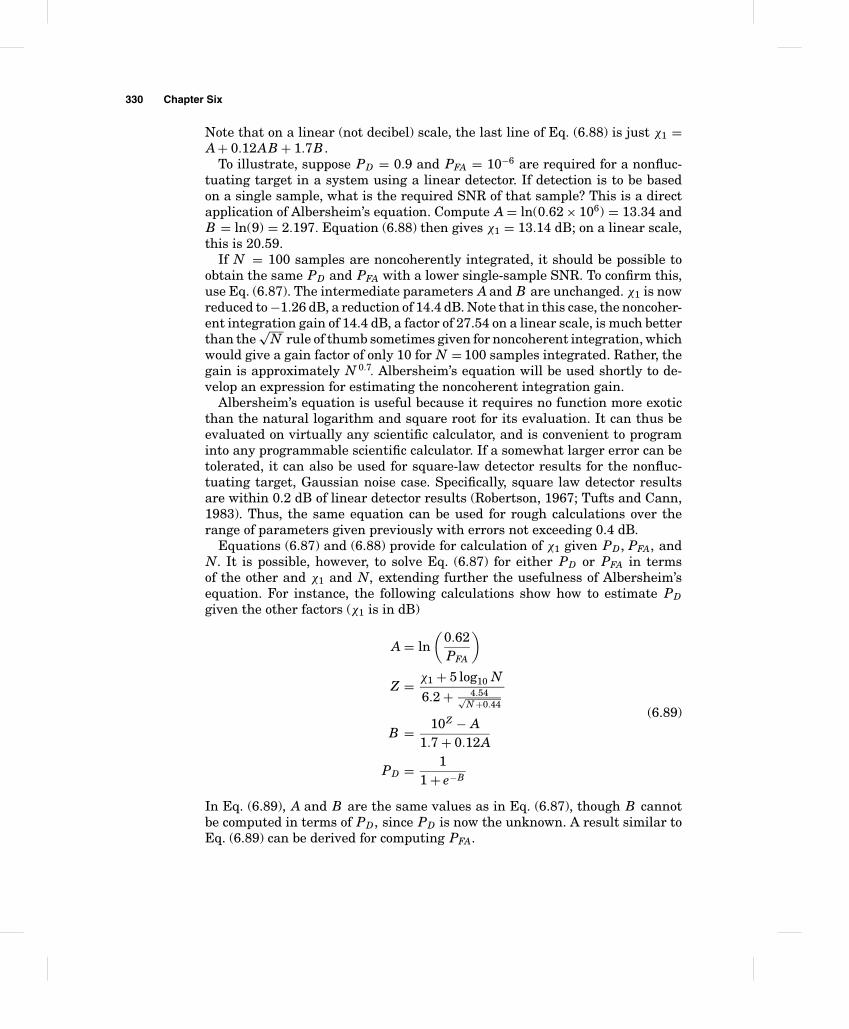
In Eq. (6.89), A and B are the same values as in Eq. (6.87), though B cannotbe computed in terms of PD, since PD is now the unknown. A result similar toEq. (6.89) can be derived for computing PFA.
Detection Fundamentals 331
Albersheim’s equation can also be used to estimate the signal-to-noise ratiogain for noncoherent integration of N samples. The noncoherent integrationgain Gnc is the reduction in single-sample SNR required to achieve a specifiedPD and PFA when N samples are combined; in dB, this is given by
Gnc(N )(dB) = χ1|1pulse − χ1|N pulses
= 5 log10 N −[6.2 +
(4.54√
N + 0.44
)]· log10( A+ 0.12AB + 1.7B )
(6.90)+ 10 log10( A+ 0.12AB + 1.7B ) dB
= 5 log10 N −[(
4.54√N + 0.44
)− 3.8
]· log10( A+ 0.12AB + 1.7B) dB
On a linear scale this becomes
Gnc(N ) =√
Nk f (N ) (6.91)
where k = A+ 0.12AB + 1.7B(6.92)
f (N ) =(
0.454√N + 0.44
)− 0.38
The constant k absorbs terms that are not a function of N, and the term f (N )is a slowly declining function of N.
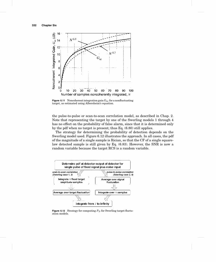
Figure 6.11 plots this estimate of Gnc in decibels for Albersheim’s nonfluc-tuating, linear detector case as a function of N. Also shown are curves corre-sponding to N 0.7 and N 0.8. The noncoherent gain is slightly better than N 0.8
for very few samples integrated (N = 2 or 3), with the effective exponent on Ndeclining slowly as N increases. Gnc is bracketed by N 0.7 and N 0.8 to in excessof N = 100 samples integrated; the gain eventually slows asymptotically tobecome proportional to
√N for very large N. Thus, noncoherent integration is
more efficient than the√
N often attributed to it for a wide range of N, butremains less efficient than coherent integration, which achieves an integra-tion gain of N. Nonetheless, its much simpler implementation, not requiringknowledge of the phase, means it is widely used to improve the SNR before thethreshold detector.
6.3.4 Fluctuating targets
The analysis in the preceding section considered only nonfluctuating targets,often called the “Swerling 0” or “Swerling 5” case. A more realistic model allowsfor target fluctuations, in which the target RCS is drawn from either the expo-nential or chi-square pdf, and the RCS of a group of N samples follows either
332 Chapter Six
Figure 6.11 Noncoherent integration gain Gnc for a nonfluctuatingtarget, as estimated using Albersheim’s equation.
the pulse-to-pulse or scan-to-scan correlation model, as described in Chap. 2.Note that representing the target by one of the Swerling models 1 through 4has no effect on the probability of false alarm, since that it is determined onlyby the pdf when no target is present; thus Eq. (6.80) still applies.
The strategy for determining the probability of detection depends on theSwerling model used. Figure 6.12 illustrates the approach. In all cases, the pdfof the magnitude of a single sample is Rician, so that the CF of a single square-law detected sample is still given by Eq. (6.83). However, the SNR is now arandom variable because the target RCS is a random variable.
Figure 6.12 Strategy for computing PD for Swerling target fluctu-ation models.
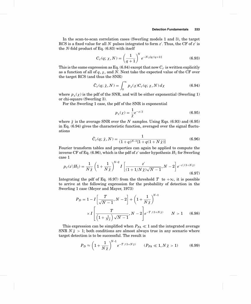
Detection Fundamentals 333
In the scan-to-scan correlation cases (Swerling models 1 and 3), the targetRCS is a fixed value for all N pulses integrated to form z′. Thus, the CF of z′ isthe N-fold product of Eq. (6.83) with itself
Cz′ (q; χ , N ) =(
1q + 1
)N
e−N χ [q/(q+1)] (6.93)
This is the same expression as Eq. (6.84) except that now Cz′ is written explicitlyas a function of all of q, χ , and N. Next take the expected value of the CF overthe target RCS (and thus the SNR)
Cz′ (q; χ , N ) =∫ ∞
0pχ (χ )Cz′ (q; χ , N ) dχ (6.94)
where pχ (χ ) is the pdf of the SNR, and will be either exponential (Swerling 1)or chi-square (Swerling 3).
For the Swerling 1 case, the pdf of the SNR is exponential
pχ (χ ) = 1χ
e−χ/χ (6.95)
where χ is the average SNR over the N samples. Using Eqs. (6.93) and (6.95)in Eq. (6.94) gives the characteristic function, averaged over the signal fluctu-ations
Cz′ (q; χ , N ) = 1(1 + q)N−1[1 + q(1 + N χ )]
(6.96)
Fourier transform tables and properties can again be applied to compute theinverse CF of Eq. (6.96), which is the pdf of z′ under hypothesis H1 for Swerlingcase 1
pz′ (z′|H1) = 1N χ
(1 + 1
N χ
)N−2
I[
z′
(1 + 1/N χ )√
N − 1, N − 2
]e−z′/(1+N χ )
(6.97)
Integrating the pdf of Eq. (6.97) from the threshold T to +∞, it is possibleto arrive at the following expression for the probability of detection in theSwerling 1 case (Meyer and Mayer, 1973)
PD = 1 − I[
T√N − 1
, N − 2]
+(
1 + 1N χ
)N−1
× I
T(
1 + 1N χ
)√N − 1
, N − 2
e−T /(1+N χ ) N > 1 (6.98)
This expression can be simplified when PFA � 1 and the integrated averageSNR N χ > 1; both conditions are almost always true in any scenario wheretarget detection is to be successful. The result is
PD ≈(
1 + 1N χ
)N−1
e−T /(1+N χ ) (PFA � 1, N χ > 1) (6.99)
334 Chapter Six
Furthermore, Eq. (6.99) is exact when N = 1; in this case it reduces to
PD = e−T /(1+χ ) (6.100)
(Note that when there is only one pulse, the average SNR χ is just the single-pulse SNR χ .) For the N = 1 case, Eq. (6.82) can then be used in Eq. (6.100) towrite a direct relationship between PD and PFA
PD = (PFA)1/(1+χ ) (6.101)
In the Swerling 2 or 4 cases, the samples exhibit pulse-to-pulse correlation,meaning they are in fact uncorrelated with one another. In this case, each ofthe N samples integrated has a different value of SNR. Consequently, it isappropriate to average over the SNR in the single-sample CF
Cr (q; χ ) =(
1q + 1
)∫ ∞
0pχ (χ )e−χ
(q
q+1
)dχ (6.102)
and then perform the N -fold multiplication of the averaged single-sample CFto get the CF of the integrated data
Cz′ (q; χ , N ) = [C(q; χ )]N (6.103)
For the Swerling 2 case specifically, the exponential pdf can again be used forthe SNR (Eq. (6.95)), applying it this time in Eq. (6.102) to arrive at
Cr (q; χ ) = 1[1 + q(1 + χ )]
(6.104)
and thus
Cz′ (q; χ , N ) = 1[1 + q(1 + χ )]N (6.105)
Inverse transforming Eq. (6.105) gives the pdf of z′ under hypothesis H1 forSwerling case 2
pz′ (z′|H1) = z′N−1e−z′/(1+χ )
(1 + χ )N (N − 1)!(6.106)
Integrating Eq. (6.106) gives the probability of detection, which can be shownto be (Meyer and Mayer, 1973)
PD = 1 − I[
T
(1 + χ )√
N, N − 1
]
= e−T /(1+χ )N−1∑l=0
1l!
(T
1 + χ
)l
(6.107)
The series approximation in the second line of Eq. (6.107) provides a convenientcomputational implementation.
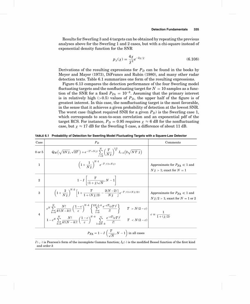
Detection Fundamentals 335
Results for Swerling 3 and 4 targets can be obtained by repeating the previousanalyses above for the Swerling 1 and 2 cases, but with a chi-square instead ofexponential density function for the SNR
pχ (χ ) = 4χ
χ2 e−2χ/χ (6.108)
Derivations of the resulting expressions for PD can be found in the books byMeyer and Mayer (1973), DiFranco and Rubin (1980), and many other radardetection texts. Table 6.1 summarizes one form of the resulting expressions.
Figure 6.13 compares the detection performance of the four Swerling modelfluctuating targets and the nonfluctuating target for N = 10 samples as a func-tion of the SNR for a fixed PFA = 10−8. Assuming that the primary interestis in relatively high (>0.5) values of PD, the upper half of the figure is ofgreatest interest. In this case, the nonfluctuating target is the most favorable,in the sense that it achieves a given probability of detection at the lowest SNR.The worst case (highest required SNR for a given PD) is the Swerling case 1,which corresponds to scan-to-scan correlation and an exponential pdf of thetarget RCS. For instance, PD = 0.95 requires χ ≈ 6 dB for the nonfluctuatingcase, but χ ≈ 17 dB for the Swerling 5 case, a difference of about 11 dB.
TABLE 6.1 Probability of Detection for Swerling Model Fluctuating Targets with a Square-Law Detector
Case PD Comments
0 or 5 QM(√
2N χ ,√
2T)
+ e−(T +N χ )N∑
r =2
(T
N χ
)r−12
Ir−1(
2√
N T χ)
1(
1 + 1N χ
)N−1
e−T /(1+N χ ) Approximate for PFA � 1 and
N χ > 1; exact for N = 1
2 1 − I
[T
(1 + χ )√
N, N − 1
]
3(
1 + 2N χ
)N−2 [1 + T
1 + (N χ/2)− 2(N −2)
N χ
]e−T /(1+(N χ/2)) Approximate for PFA � 1 and
N χ/2 > 1; exact for N = 1 or 2
4
cNN∑
k=0
N !k!(N − k)!
(1 − c
c
)N−k{
2N−1−k∑l=0
e−cT(cT )l
l!
}T > N (2 − c)
1 − cNN∑
k=0
N !k!(N − k)!
(1 − c
c
)N−k ∞∑l=2N−k
e−cT(cT )l
l!T < N (2 − c)
c ≡ 11 + (χ/2)
PFA = 1 − I(
T√N
, N − 1)
in all cases
I (·, ·) is Pearson’s form of the incomplete Gamma function; Ik(·) is the modified Bessel function of the first kindand order k
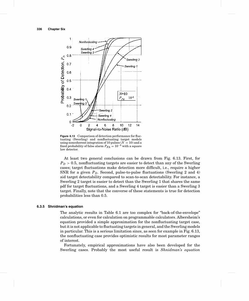
336 Chapter Six
Figure 6.13 Comparison of detection performance for fluc-tuating (Swerling) and nonfluctuating target modelsusing noncoherent integration of 10 pulses (N = 10) and afixed probability of false alarm PFA = 10−8 with a squarelaw detector.
At least two general conclusions can be drawn from Fig. 6.13. First, forPD > 0.5, nonfluctuating targets are easier to detect than any of the Swerlingcases; target fluctuations make detection more difficult, i.e., require a higherSNR for a given PD. Second, pulse-to-pulse fluctuations (Swerling 2 and 4)aid target detectability compared to scan-to-scan detectability. For instance, aSwerling 2 target is easier to detect than the Swerling 1 that shares the samepdf for target fluctuations, and a Swerling 4 target is easier than a Swerling 3target. Finally, note that the converse of these statements is true for detectionprobabilities less than 0.5.
6.3.5 Shnidman’s equation
The analytic results in Table 6.1 are too complex for “back-of-the-envelope”calculations, or even for calculation on programmable calculators. Albersheim’sequation provided a simple approximation for the nonfluctuating target case,but it is not applicable to fluctuating targets in general, and the Swerling modelsin particular. This is a serious limitation since, as seen for example in Fig. 6.13,the nonfluctuating case provides optimistic results for most parameter rangesof interest.
Fortunately, empirical approximations have also been developed for theSwerling cases. Probably the most useful result is Shnidman’s equation
Detection Fundamentals 337
(Shnidman, 2002). Similar to Albersheim’s equation, this series of equationsgives the single-pulse SNR χ required to achieve a specified PD and PFA withnoncoherent integration of N samples. Unlike Albersheim’s equation, the re-sults are for a square law detector; however, as noted previously, the differencesare small and in any event, the square law detector is used as much or morethan a linear detector.
Shnidman’s “equation” is given by the following series of calculations
K =
∞, nonfluctuating target (“Swerling 0 / 5”)1, Swerling 1N , Swerling 22, Swerling 32N Swerling 4
α ={
0 N < 4014 N ≥ 40
(6.109)
η =√
−0.8 ln(4PFA(1 − PFA)) + sign(PD − 0.5)√
−0.8 ln(4PD(1 − PD))
X∞ = η
(η + 2
√N2
+(
α − 14
))(6.110)
C1 = {[(17.7006PD − 18.4496)PD + 14.5339]PD − 3.525}/K
C2 = 1K
{exp(27.31PD − 25.14) + (PD − 0.8)
[0.7 ln
(10−5
PFA
)+ (2N − 20)
80
]}
CdB ={
C1 0.1 ≤ PD ≤ 0.872
C1 + C2 0.872 < PD ≤ 0.99
C = 10CdB/10 (6.111)
χ1 = C · X∞N
χ1 (dB) = 10 log10(χ1) (6.112)
Note that several of the equations simplify in the nonfluctuating case, K = ∞.Specifically, in this case C1 = C2 = 0, so that in turn CdB = 0 and C = 1. Thefunction sign(x) is +1 if x > 0 and −1 if x < 0.
The accuracy bounds on Shnidman’s equation are somewhat looser than thosespecified for Albersheim’s equation. Specifically, except at the extreme valuesof PD for the Swerling 1 case, the error in the estimate of χ1 is less than 0.5 dBfor 0.1 ≤ PD ≤ 0.99, 10−9 ≤ PFA ≤ 10−3, and 1 ≤ N ≤ 100. This is a much betterrange for PD than used in Albersheim’s equation. The range of N is muchsmaller, but still large enough for almost all problems of interest. Figure 6.14illustrates the error in the estimate of the single-pulse SNR χ1 using Shnid-man’s equation for the case PFA = 10−6 and N = 5, and for PD over the specifiedrange of 0.1 to 0.99.
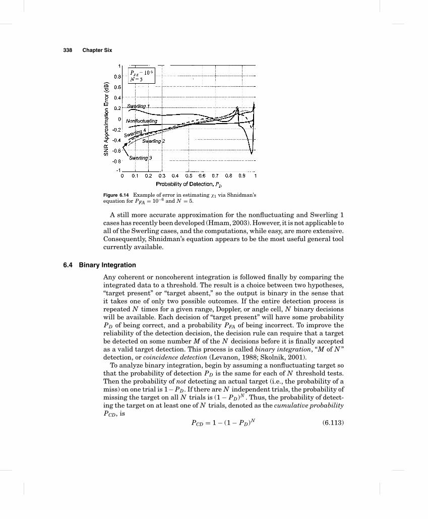
338 Chapter Six
Figure 6.14 Example of error in estimating χ1 via Shnidman’sequation for PFA = 10−6 and N = 5.
A still more accurate approximation for the nonfluctuating and Swerling 1cases has recently been developed (Hmam, 2003). However, it is not applicable toall of the Swerling cases, and the computations, while easy, are more extensive.Consequently, Shnidman’s equation appears to be the most useful general toolcurrently available.
6.4 Binary Integration
Any coherent or noncoherent integration is followed finally by comparing theintegrated data to a threshold. The result is a choice between two hypotheses,“target present” or “target absent,” so the output is binary in the sense thatit takes one of only two possible outcomes. If the entire detection process isrepeated N times for a given range, Doppler, or angle cell, N binary decisionswill be available. Each decision of “target present” will have some probabilityPD of being correct, and a probability PFA of being incorrect. To improve thereliability of the detection decision, the decision rule can require that a targetbe detected on some number M of the N decisions before it is finally acceptedas a valid target detection. This process is called binary integration, “M of N ”detection, or coincidence detection (Levanon, 1988; Skolnik, 2001).
To analyze binary integration, begin by assuming a nonfluctuating target sothat the probability of detection PD is the same for each of N threshold tests.Then the probability of not detecting an actual target (i.e., the probability of amiss) on one trial is 1− PD. If there are N independent trials, the probability ofmissing the target on all N trials is (1 − PD)N . Thus, the probability of detect-ing the target on at least one of N trials, denoted as the cumulative probabilityPCD, is
PCD = 1 − (1 − PD)N (6.113)
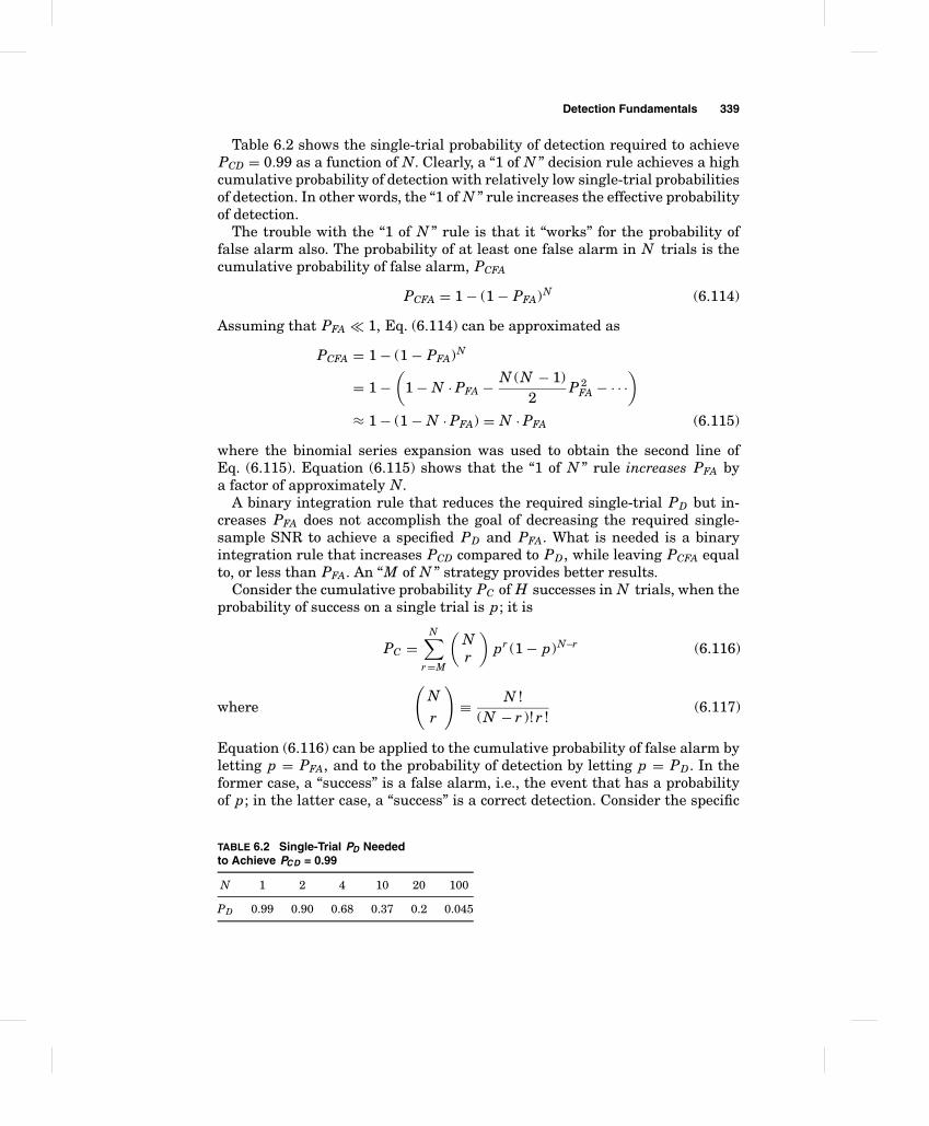
Detection Fundamentals 339
Table 6.2 shows the single-trial probability of detection required to achievePCD = 0.99 as a function of N. Clearly, a “1 of N ” decision rule achieves a highcumulative probability of detection with relatively low single-trial probabilitiesof detection. In other words, the “1 of N ” rule increases the effective probabilityof detection.
The trouble with the “1 of N ” rule is that it “works” for the probability offalse alarm also. The probability of at least one false alarm in N trials is thecumulative probability of false alarm, PCFA
PCFA = 1 − (1 − PFA)N (6.114)
Assuming that PFA � 1, Eq. (6.114) can be approximated as
PCFA = 1 − (1 − PFA)N
= 1 −(
1 − N · PFA − N (N − 1)2
P 2FA − · · ·
)≈ 1 − (1 − N · PFA) = N · PFA (6.115)
where the binomial series expansion was used to obtain the second line ofEq. (6.115). Equation (6.115) shows that the “1 of N ” rule increases PFA bya factor of approximately N.
A binary integration rule that reduces the required single-trial PD but in-creases PFA does not accomplish the goal of decreasing the required single-sample SNR to achieve a specified PD and PFA. What is needed is a binaryintegration rule that increases PCD compared to PD, while leaving PCFA equalto, or less than PFA. An “M of N ” strategy provides better results.
Consider the cumulative probability PC of H successes in N trials, when theprobability of success on a single trial is p; it is
PC =N∑
r =M
(Nr
)pr (1 − p)N−r (6.116)
where
(Nr
)≡ N !
(N − r )! r !(6.117)
Equation (6.116) can be applied to the cumulative probability of false alarm byletting p = PFA, and to the probability of detection by letting p = PD. In theformer case, a “success” is a false alarm, i.e., the event that has a probabilityof p; in the latter case, a “success” is a correct detection. Consider the specific
TABLE 6.2 Single-Trial PD Neededto Achieve PCD = 0.99
N 1 2 4 10 20 100
PD 0.99 0.90 0.68 0.37 0.2 0.045
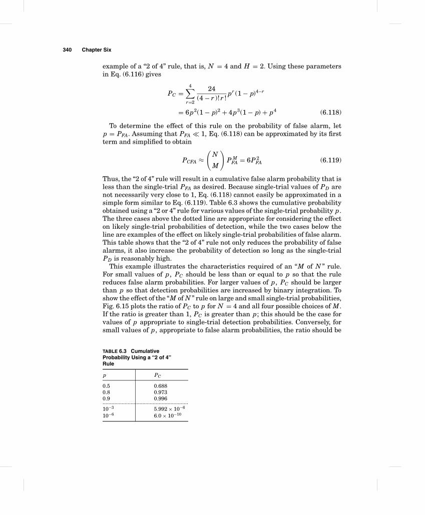
340 Chapter Six
example of a “2 of 4” rule, that is, N = 4 and H = 2. Using these parametersin Eq. (6.116) gives
PC =4∑
r=2
24(4 − r )! r !
pr (1 − p)4−r
= 6p2(1 − p)2 + 4p3(1 − p) + p4 (6.118)
To determine the effect of this rule on the probability of false alarm, letp = PFA. Assuming that PFA � 1, Eq. (6.118) can be approximated by its firstterm and simplified to obtain
PCFA ≈(
N
M
)P M
FA = 6P 2FA (6.119)
Thus, the “2 of 4” rule will result in a cumulative false alarm probability that isless than the single-trial PFA as desired. Because single-trial values of PD arenot necessarily very close to 1, Eq. (6.118) cannot easily be approximated in asimple form similar to Eq. (6.119). Table 6.3 shows the cumulative probabilityobtained using a “2 or 4” rule for various values of the single-trial probability p.The three cases above the dotted line are appropriate for considering the effecton likely single-trial probabilities of detection, while the two cases below theline are examples of the effect on likely single-trial probabilities of false alarm.This table shows that the “2 of 4” rule not only reduces the probability of falsealarms, it also increase the probability of detection so long as the single-trialPD is reasonably high.
This example illustrates the characteristics required of an “M of N ” rule.For small values of p, PC should be less than or equal to p so that the rulereduces false alarm probabilities. For larger values of p, PC should be largerthan p so that detection probabilities are increased by binary integration. Toshow the effect of the “M of N ” rule on large and small single-trial probabilities,Fig. 6.15 plots the ratio of PC to p for N = 4 and all four possible choices of M.If the ratio is greater than 1, PC is greater than p; this should be the case forvalues of p appropriate to single-trial detection probabilities. Conversely, forsmall values of p, appropriate to false alarm probabilities, the ratio should be
TABLE 6.3 CumulativeProbability Using a “2 of 4”Rule
p PC
0.5 0.6880.8 0.9730.9 0.996..........................................................10−3 5.992 × 10⁻⁶
10−6 6.0 × 10⁻¹⁰
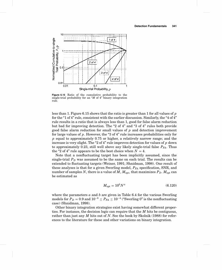
Detection Fundamentals 341
Figure 6.15 Ratio of the cumulative probability to thesingle-trial probability for an “M of 4” binary integrationrule.
less than 1. Figure 6.15 shows that the ratio is greater than 1 for all values of pfor the “1 of 4” rule, consistent with the earlier discussion. Similarly, the “4 of 4”rule results in a ratio that is always less than 1, good for false alarm reductionbut bad for improving detection. The “2 of 4” and “3 of 4” rules both providegood false alarm reduction for small values of p and detection improvementfor large values of p. However, the “3 of 4” rule increases probabilities only forp equal to approximately 0.75 or higher, a relatively narrow range; and theincrease is very slight. The “2 of 4” rule improves detection for values of p downto approximately 0.23, still well above any likely single-trial false PFA. Thusthe “2 of 4” rule appears to be the best choice when N = 4.
Note that a nonfluctuating target has been implicitly assumed, since thesingle-trial PD was assumed to be the same on each trial. The results can beextended to fluctuating targets (Weiner, 1991; Shnidman, 1998). One result ofthese analyses is that for a given Swerling model, PFA specification, SNR, andnumber of samples N, there is a value of M, Mopt, that maximizes PD. Mopt canbe estimated as
Mopt = 10bN a (6.120)
where the parameters a and b are given in Table 6.4 for the various Swerlingmodels for PD = 0.9 and 10−8 ≤ PFA ≤ 10−4 (“Swerling 0” is the nonfluctuatingcase) (Shnidman, 1998).
Other binary integration strategies exist having somewhat different proper-ties. For instance, the decision logic can require that the M hits be contiguous,rather than just any M hits out of N. See the book by Skolnik (1988) for refer-ences to the literature for these and other variations on binary integration.
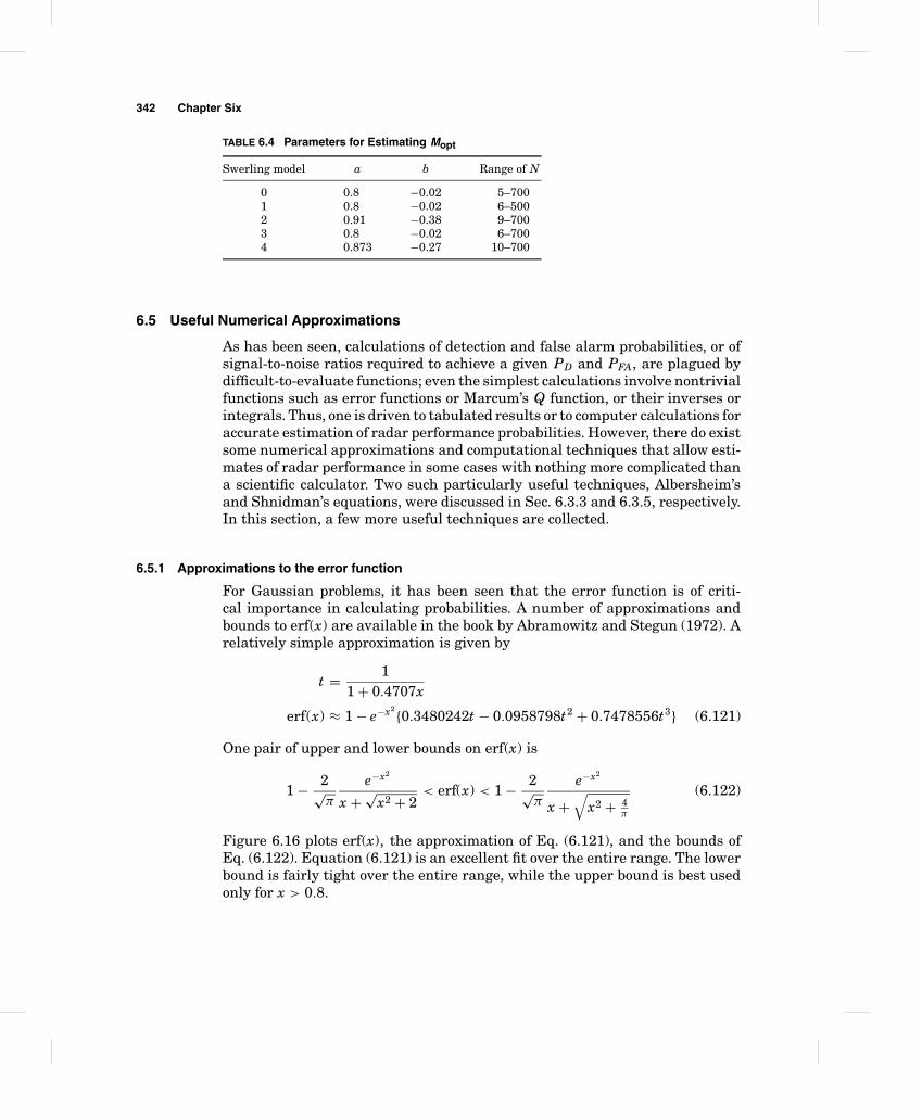
342 Chapter Six
TABLE 6.4 Parameters for Estimating Mopt
Swerling model a b Range of N
0 0.8 −0.02 5–7001 0.8 −0.02 6–5002 0.91 −0.38 9–7003 0.8 −0.02 6–7004 0.873 −0.27 10–700
6.5 Useful Numerical Approximations
As has been seen, calculations of detection and false alarm probabilities, or ofsignal-to-noise ratios required to achieve a given PD and PFA, are plagued bydifficult-to-evaluate functions; even the simplest calculations involve nontrivialfunctions such as error functions or Marcum’s Q function, or their inverses orintegrals. Thus, one is driven to tabulated results or to computer calculations foraccurate estimation of radar performance probabilities. However, there do existsome numerical approximations and computational techniques that allow esti-mates of radar performance in some cases with nothing more complicated thana scientific calculator. Two such particularly useful techniques, Albersheim’sand Shnidman’s equations, were discussed in Sec. 6.3.3 and 6.3.5, respectively.In this section, a few more useful techniques are collected.
6.5.1 Approximations to the error function
For Gaussian problems, it has been seen that the error function is of criti-cal importance in calculating probabilities. A number of approximations andbounds to erf(x) are available in the book by Abramowitz and Stegun (1972). Arelatively simple approximation is given by
t = 11 + 0.4707x
erf(x) ≈ 1 − e−x2{0.3480242t − 0.0958798t2 + 0.7478556t3} (6.121)
One pair of upper and lower bounds on erf(x) is
1 − 2√π
e−x2
x + √x2 + 2
< erf(x) < 1 − 2√π
e−x2
x +√
x2 + 4π
(6.122)
Figure 6.16 plots erf(x), the approximation of Eq. (6.121), and the bounds ofEq. (6.122). Equation (6.121) is an excellent fit over the entire range. The lowerbound is fairly tight over the entire range, while the upper bound is best usedonly for x > 0.8.
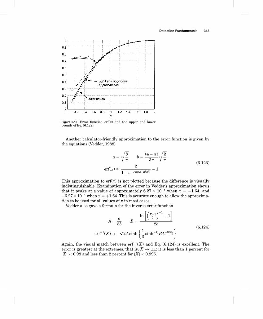
Detection Fundamentals 343
Figure 6.16 Error function erf(x) and the upper and lowerbounds of Eq. (6.122).
Another calculator-friendly approximation to the error function is given bythe equations (Vedder, 1988)
a =√
8π
b = (4 − π )3π
√2π
(6.123)erf(x) ≈ 2
1 + e−√
2x(a+2bx2)− 1
This approximation to erf(x) is not plotted because the difference is visuallyindistinguishable. Examination of the error in Vedder’s approximation showsthat it peaks at a value of approximately 6.27 × 10⁻⁴ when x = −1.64, and−6.27×10⁻⁴ when x = +1.64. This is accurate enough to allow the approxima-tion to be used for all values of x in most cases.
Vedder also gave a formula for the inverse error function
A = a3b
B =ln[(
X+12
)−1− 1]
2b(6.124)
erf−1(X ) ≈ −√
2Asinh{
13
sinh−1(BA−3/2)}
Again, the visual match between erf−1(X ) and Eq. (6.124) is excellent. Theerror is greatest at the extremes, that is, X → ±1; it is less than 1 percent for|X | < 0.98 and less than 2 percent for |X | < 0.995.
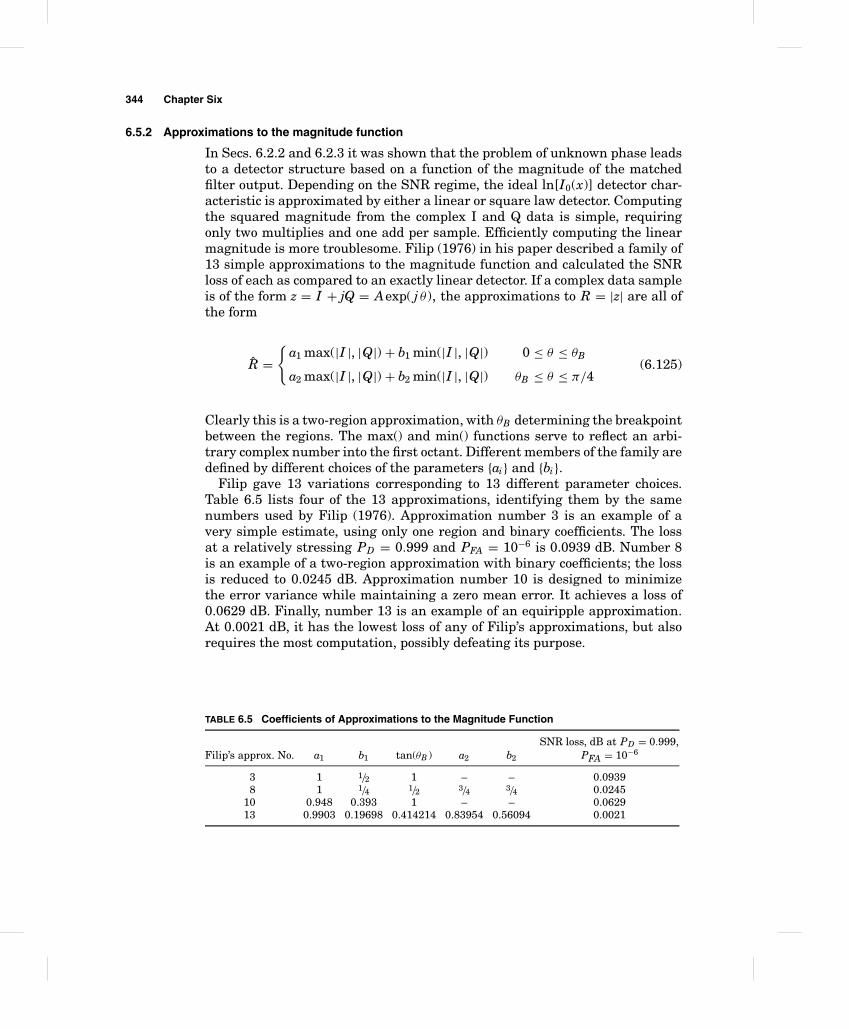
344 Chapter Six
6.5.2 Approximations to the magnitude function
In Secs. 6.2.2 and 6.2.3 it was shown that the problem of unknown phase leadsto a detector structure based on a function of the magnitude of the matchedfilter output. Depending on the SNR regime, the ideal ln[I0(x)] detector char-acteristic is approximated by either a linear or square law detector. Computingthe squared magnitude from the complex I and Q data is simple, requiringonly two multiplies and one add per sample. Efficiently computing the linearmagnitude is more troublesome. Filip (1976) in his paper described a family of13 simple approximations to the magnitude function and calculated the SNRloss of each as compared to an exactly linear detector. If a complex data sampleis of the form z = I + jQ = Aexp( j θ ), the approximations to R = |z| are all ofthe form
R ={
a1 max(|I |, |Q|) + b1 min(|I |, |Q|) 0 ≤ θ ≤ θB
a2 max(|I |, |Q|) + b2 min(|I |, |Q|) θB ≤ θ ≤ π/4(6.125)
Clearly this is a two-region approximation, with θB determining the breakpointbetween the regions. The max() and min() functions serve to reflect an arbi-trary complex number into the first octant. Different members of the family aredefined by different choices of the parameters {ai} and {bi}.
Filip gave 13 variations corresponding to 13 different parameter choices.Table 6.5 lists four of the 13 approximations, identifying them by the samenumbers used by Filip (1976). Approximation number 3 is an example of avery simple estimate, using only one region and binary coefficients. The lossat a relatively stressing PD = 0.999 and PFA = 10−6 is 0.0939 dB. Number 8is an example of a two-region approximation with binary coefficients; the lossis reduced to 0.0245 dB. Approximation number 10 is designed to minimizethe error variance while maintaining a zero mean error. It achieves a loss of0.0629 dB. Finally, number 13 is an example of an equiripple approximation.At 0.0021 dB, it has the lowest loss of any of Filip’s approximations, but alsorequires the most computation, possibly defeating its purpose.
TABLE 6.5 Coefficients of Approximations to the Magnitude Function
SNR loss, dB at PD = 0.999,Filip’s approx. No. a1 b1 tan(θB ) a2 b2 PFA = 10−6
3 1 1/2 1 – – 0.09398 1 1/4 1/2 3/4 3/4 0.0245
10 0.948 0.393 1 – – 0.062913 0.9903 0.19698 0.414214 0.83954 0.56094 0.0021
Detection Fundamentals 345
References
Abramowitz, M., and I. A. Stegun, Handbook of Mathematical Functions with Formulas,Graphs, and Mathematical Tables. National Bureau of Standards, U.S. Dept. of Commerce,1972.
Albersheim, W. J., “Closed-Form Approximation to Robertson’s Detection Characteristics,” Proceed-ings of IEEE, vol. 69, no. 7, p. 839, July 1981.
Brennan, L. E., and I. S. Reed, “A Recursive Method of Computing the Q Function,” IEEE Trans-actions on Information Theory, vol. IT-11, no. 2, pp. 312–313, April 1965.
Cantrell, P. E., and A. K. Ojha, “Comparison of Generalized Q-function Algorithms,” IEEE Trans-actions on Information Theory, vol. IT-33, no. 4, pp. 591–596, July 1987.
DiFranco, J. V., and W. L. Rubin, Radar Detection. Artech House, Dedham, MA, 1980.Filip, A. E., “A Baker’s Dozen Magnitude Approximations and Their Detection Statistics,”
IEEE Transactions on Aerospace & Electronic Systems, vol. AES-12, no. 1, pp. 86–89,Jan. 1976.
Hmam, H., “Approximating the SNR Value in Detection Problems,” IEEE Transactions on Aerospaceand Electronic Systems, vol. AES-39, no. 4, pp. 1446–1452, Oct. 2003.
Johnson, D. H., and D. E. Dudgeon, Array Signal Processing. Prentice Hall, Englewood Cliffs, NJ,1993.
Kay, S. M., Fundamentals of Statistical Signal Processing, Vol. I: Estimation Theory. Prentice Hall,Upper Saddle River, NJ, 1993.
Kay, S. M., Fundamentals of Statistical Signal Processing, Vol. II: Detection Theory. Prentice Hall,Upper Saddle River, NJ, 1998.
Levanon, N., Radar Principles. Wiley, New York, 1988.Meyer, D. P., and H. A. Mayer, Radar Target Detection. Academic Press, New York, 1973.Papoulis, A., Probability, Random Variables, and Stochastic Processes, 2d ed. McGraw-Hill, New
York, 1984.Robertson, G. H., “Operating Characteristic for a Linear Detector of CW Signals in Narrow
Band Gaussian Noise,” Bell System Technical Journal, vol. 46, no. 4, pp. 755–774, April1967.
Shnidman, D. A., “Radar Detection Probabilities and Their Calculation,” IEEE Transactions onAerospace and Electronic Systems, vol. AES-31, no. 3, pp. 928–950, July 1995.
Shnidman, D. A., “Binary Integration for Swerling Target Fluctuations,” IEEE Transactions onAerospace and Electronic Systems, vol. AES-34, no. 3, pp. 1043–1053, July 1998.
Shnidman, D. A., “Determination of Required SNR Values,” IEEE Transactions on Aerospace andElectronic Systems, vol. AES-38, no. 3, pp. 1059–1064, July 2002.
Skolnik, M. I., Introduction to Radar Systems, 3d ed. McGraw-Hill, New York, 2001.Tufts, D. W., and A. J. Cann, “On Albersheim’s Detection Equation,” IEEE Transactions on
Aerospace and Electronic Systems, vol. AES-19, no. 4, pp. 643–646, July 1983.Van Trees, H. L., Detection, Estimation, and Modulation Theory, Part I: Detection, Estimation, and
Linear Modulation Theory. Wiley, New York, 1968.Vedder, J. D., “Approximation to the Normal Probability Distribution,” NASA Tech Briefs, p. 96,
Feb. 1988.Weiner, M. A., “Binary Integration of Fluctuating Targets,” IEEE Transactions on Aerospace and
Electronic Systems, vol. AES-27, no. 1, pp. 11–17, Jan. 1991.

346


![Naruto v02 c06 [animakong]](https://img.dokumen.tips/doc/110x75/55cd2c01bb61eb07048b4602/naruto-v02-c06-animakong.jpg)