Reviews inComputationalChemistryVolume 17

Reviews in Computational Chemistry, Volume 17. Edited by Kenny B. Lipkowitz, Donald B. BoydCopyright 2001 John Wiley & Sons, Inc.

ISBNs: 0-471-39845-4 (Hardcover); 0-471-22441-3 (Electronic)

Reviews inComputationalChemistryVolume 17

Edited by

Kenny B. Lipkowitz and Donald B. Boyd

NEW YORK CHICHESTER WEINHEIM BRISBANE SINGAPORE TORONTO

Designations used by companies to distinguish their products are often claimed as trademarks.In all instances where John Wiley & Sons, Inc., is aware of a claim, the product names appearin initial capital or ALL CAPITAL LETTERS. Readers, however, should contact the appropriatecompanies for more complete information regarding trademarks and registration.

Copyright 2001 by John Wiley & Sons, Inc. All rights reserved.

No part of this publication may be reproduced, stored in a retrieval system or transmitted in anyform or by any means, electronic or mechanical, including uploading, downloading, printing,decompiling, recording or otherwise, except as permitted under Sections 107 or 108 of the 1976United States Copyright Act, without the prior written permission of the Publisher. Requests to thePublisher for permission should be addressed to the Permissions Department, John Wiley & Sons,Inc., 605 Third Avenue, New York, NY 10158-0012, (212) 850-6011, fax (212) 850-6008,E-Mail: PERMREQ @ WILEY.COM.

This publication is designed to provide accurate and authoritative information in regard to thesubject matter covered. It is sold with the understanding that the publisher is not engaged inrendering professional services. If professional advice or other expert assistance is required, theservices of a competent professional person should be sought.

ISBN 0-471-22441-3

This title is also available in print as ISBN 0-471-39845-4.

For more information about Wiley products, visit our web site at www.Wiley.com.

Preface

The aphorism ‘‘Knowledge is power’’ applies to diverse circumstances.Anyone who has climbed an organizational ladder during a career understandsthis concept and knows how to exploit it. The problem for scientists, however,is that there may exist too much to know, overwhelming even the brightestintellectual. Indeed, it is a struggle for most scientists to assimilate even atiny part of what is knowable. Scientists, especially those in industry, areunder enormous pressure to know more sooner. The key to using knowl-edge to gain power is knowing what to know, which is often a questionof what some might call, variously, innate leadership ability, intuition, orluck.

Attempts to manage specialized scientific information have given birth tothe new discipline of informatics. The branch of informatics that deals primar-ily with genomic (sequence) data is bioinformatics, whereas cheminformaticsdeals with chemically oriented data. Informatics examines the way peoplework with computer-based information. Computers can access huge ware-houses of information in the form of databases. Effective mining of these data-bases can, in principle, lead to knowledge.

In the area of chemical literature information, the largest databases areproduced by the Chemical Abstracts Service (CAS) of the American ChemicalSociety (ACS). As detailed on their website (www.cas.org), their principaldatabases are the Chemical Abstracts database (CA) with 16 million docu-ment records (mainly abstracts of journal articles and other literature) andthe REGISTRY database with more than 28 million substance records. Inan earlier volume of this series,* we discussed CAS’s SciFinder software formining these databases. SciFinder is a tool for helping people formulatequeries and view hits. SciFinder does not have all the power and precisionof the command-line query system of CAS’s STN, a software system developedearlier to access these and other CAS databases. But with SciFinder being easy

*D. B. Boyd and K. B. Lipkowitz, in Reviews in Computational Chemistry, K. B. Lipkowitzand D. B. Boyd, Eds., Wiley-VCH, New York, 2000, Vol. 15, pp. v–xxxv. Preface.

v

to use and with favorable academic pricing from CAS, now many institutionshave purchased it.

This volume of Reviews in Computational Chemistry includes an appen-dix with a lengthy compilation of books on the various topics in computa-tional chemistry. We undertook this task because as editors we wereoccasionally asked whether such a listing existed. No satisfactory list couldbe found, so we developed our own using SciFinder, supplemented with otherresources.

We were anticipating not being able to retrieve every book we were look-ing for with SciFinder, but we were surprised at how many omissions wereencountered. For example, when searching specifically for our own book ser-ies, Reviews in Computational Chemistry, several of the existing volumes werenot ‘‘hit.’’ Moreover, these were not consecutive omissions like Volumes 2–5,but rather they were missing sporadically. Clearly, something about the data-base is amiss.

Whereas experienced chemistry librarians and information specialistsmay fully appreciate the limitations of the CAS databases, a less experienceduser may wonder: How punctilious are the data being mined by SciFinder?Certainly, for example, one could anticipate differences in spelling likeMueller versus Muller, so that typing in only Muller would lead one to notfinding the former name. The developers of SciFinder foresaw this problem,and the software does give the user the option to look for names that arespelled similarly. Thus, there is some degree of ‘‘fuzzy logic’’ implementedin the search algorithms. However, when there are misses of informationthat should be in the database, the searches are either not fuzzy enough orthere may be wrong or incomplete data in the CAS databases. Presumably,these errors were generated by the CAS staff during the process of data entry.In any event, there are errors, and we were curious how prevalent they are.

To probe this, we analyzed the hits from our SciFinder searches. Threekinds of errors were considered: (1) wrong, meaning there were factual errorsin an entry which prevented the citation from being found by, say, an authorsearch (although more exhaustive mining of the database did eventuallyuncover the entry); (2) incomplete, meaning that a hit could be obtained,but there were missing pieces of data, for example, the publisher, the city ofpublication, the year of publication, or the name of an author or editor; (3)spelling, meaning that there were spelling or typographical errors apparentin the entry, but the hit could nevertheless be found with SciFinder. In ourstudy, about 95% of the books abstracted in the CA database were satisfac-tory; 1% had errors that could be ascribed to the data being wrong, 3% hadincomplete data, and 1% had spelling errors. These error rates are lower lim-its. There almost certainly exist errors in spellings of authors’ names or othererrors that we did not detect. Concerning the wrong entries, most of themwere recognized with the help of books on our bookshelves, but there areprobably others we did not notice. Many errors, such as missing volumes of

vi Preface

a series, became evident when books from the same author or on the sametopic were listed together.

If we noticed a variation of the spelling of an author’s name from yearto year or from edition to edition, especially when Russian and EasternEuropean names are involved, we classified these entries as being wrong ifthe infraction is serious enough to give a wrong outcome in a search. If oneis looking for books by I. B. Golovanov and A. K. Piskunov, for example,one needs to search also for Golowanow and Piskunow, respectively. Theuser discovers that the spelling of their co-author changes from N. M. Sergeevto N. M. Sergejew! Should the user write Markovnikoff or Markovnikov?(Both spellings can be found in current undergraduate organic chemistry text-books.) More of the literature is being generated by people who have non-English names. But even for very British names, such as R. McWeeney andR. McWeeny, there are misspellings in the CAS database. Perhaps one ofthe more frequent occurrences of misspellings and errors is bestowed on N.Yngve Ohrn. Some of the CAS spellings include: N. Yngve Oehrn, YngveOhrn, Ynave Ohrn, and even Yngve Oehru! There also may be errors concern-ing the publishing houses, some not very familiar to American readers. Forexample, aside from variability in their spellings, the Polish publisher Panst-wowe Wydawnictwo Naukowe (PWN) is entered as PAN in one of the entriesof W. Kolos’ books, whereas the others are PWN.

Some of this analysis might be considered ‘‘nit-picking,’’ but an error iscertainly serious if it prevents a user from finding what is actually in the data-base. Our exercises with SciFinder suggest that it would be helpful if CASstrengthened their quality control and standardization processes. Cross-checking and cleaning up the spellings in their databases would allow usersto retrieve desired data more reliably. It would also enhance the value of theCAS databases if missing data were added retrospectively.

So, what level of data integrity is acceptable? The total percentage oferrors we found in our study was 5%. Is this satisfactory? Is this the bestwe can hope for? Hopefully not, especially as more people become dependenton databases and the rate of production of data becomes ever faster. Clearly,there is a need for a system that will better validate data being entered in themost used CAS databases. It is desirable that the quality of the databasesincreases at the same time as they are mushrooming in size.

A Tribute

Many prominent colleagues who have worked in computational chemis-try have passed away since about the time this book series began. Theseinclude (in alphabetical order) Jan Almlof, Russell J. Bacquet, Jeremy K.Burdett, Jean-Louis Calais, Michael J. S. Dewar, Russell S. Drago, KenichiFukui, Joseph Gerratt, Hans H. Jaffe, Wlodzimierz Kolos, Bowen Liu, Per-Olov Lowdin, Amatzya Y. Meyer, William E. Palke, Bernard Pullman, Robert

Preface vii

Rein, Carlo Silipo, Robert W. Taft, Antonio Vittoria, Kent R. Wilson, andMichael C. Zerner.* These scientists enriched the field of computational chem-istry each in his own way. Three of these individuals (Almlof, Wilson, Zerner)were authors of past chapters in Reviews in Computational Chemistry.

Dr. Michael C. Zerner died from cancer on February 2, 2000. Other tri-butes have already been paid to Mike, but we would like to add ours. Manyreaders of this series knew Mike personally or were aware of his research.Mike earned a B.S. degree from Carnegie Mellon University in 1961, anA.M. from Harvard University in 1962, and, under the guidance of MartinGouterman, a Ph.D. in Chemistry from Harvard in 1966. Mike then servedhis country in the United States Army, rising to the rank of Captain. Afterpostdoctoral work in Uppsala, Sweden, where he met his wife, he held facultypositions at the University of Guelph, Canada, and then at the University ofFlorida. At Gainesville he served as department chairman and was eventuallynamed distinguished professor, a position held by only 16 other faculty mem-bers on the Florida campus.

Probably, Mike’s research has most touched other scientists through hisdevelopment of ZINDO, the semiempirical molecular orbital method and

*After this volume was in press, the field of computational chemistry lost at least four morehighly esteemed contributors: G. N. Ramachandran, Gilda H. Loew, Peter A. Kollman, andDonald E. Williams. We along with many others grieve their demise, but remember theircontributions with great admiration. Professor Ramachandran lent his name to the plots fordisplaying conformational angles in peptides and proteins. Dr. Loew founded the MolecularResearch Institute in California and applied computational chemistry to drugs, proteins, andother molecules. She along with Dr. Joyce J. Kaufman were influential figures in the branchof computational chemistry called by its practitioners ‘‘quantum pharmacology’’ during the1960s and 1970s. Professor Kollman, like many in our field, began his career as a quantumchemist and then expanded his interests to include other ways of modeling molecules. Peter’swork in molecular dynamics and his AMBER program are well known and helped shape thefield as it exists today. Professor Williams, an author of a chapter in Volume 2 of Reviews inComputational Chemistry, was famed for his contributions to the computation of atomiccharges and intermolecular forces. Drs. Ramachandran, Loew, and Williams were blessedwith long careers, whereas Peter’s was cut short much too early.

Although several of Peter’s students and collaborators have written chapters for Reviewsin Computational Chemistry, Peter’s association with the book series was a review he wroteabout Volume 13. As a tribute to Peter, we would like to quote a few words from this bookreview, which appeared in J. Med. Chem., 43 (11), 2290 (2000). While always objective inhis evaluation, Peter was also generous in praise of the individual chapters (‘‘a beautifulpiece of pedagogy,’’ ‘‘timely and interesting,’’ ‘‘valuable,’’ and ‘‘an enjoyable read’’). He hadthese additional comments which we shall treasure:

This volume of Reviews in Computational Chemistry is of the samevery high standard as previous volumes. The editors have played akey role in carving out the discipline of computational chemistry, hav-ing organized a seminal symposium in 1983 and having served as thechairmen of the first Gordon Conference on Computational Chemistryin 1986. Thus, they have a broad perspective on the field, and the arti-cles in this and previous volumes reflect this.

We would like to add that Peter was an invited speaker at the Symposium on MolecularMechanics (held in Indianapolis in 1983) and was co-chairman of the second GordonResearch Conference on Computational Chemistry in 1988. As we pointed out in the Pre-face of Volume 13 (p. xiii) of this book series, no one had been cited more frequently inReviews of Computational Chemistry than Peter. Peter—and the others—will be missed.

viii Preface

program for calculating the electronic structure of molecules. To relieve theburden of providing user support, Mike let a software company commercializeit, and it is currently distributed by Accelrys (nee Molecular Simulations, Inc.)In addition, a version of the ZINDO method has been written separately byscientists at Hypercube in their modeling software HyperChem. Likewise,ZINDO calculations can be done with the CAChe (Computer-Aided Chemis-try) software distributed by Fujitsu. Several thousand academic, government,and industrial laboratories have used ZINDO in one form or another. ZINDOis even distributed by several publishing companies to accompany their text-books, including introductory texts in chemistry.

Mike published over 225 research articles in well-respected journals and20 book chapters, one of which was in the second volume of Reviews in Com-putational Chemistry. It still remains a highly cited chapter in our series. Inaddition, Mike edited 35 books or proceedings, many of which were asso-ciated with the very successful Sanibel Symposia that he helped organizewith his colleagues at Florida’s Quantum Theory Project (QTP). If you havenever organized a conference or edited a book, it may be hard to realize howmuch work is involved. Not only was Mike doing basic research, teaching(including at workshops worldwide), and serving on numerous university gov-ernance and service committees, he was also consulting for Eastman Kodak,Union Carbide, and others. A little known fact is that Mike is a co-inventorof eight patents related to polymers and polymer coatings.

Mike’s interests and abilities earned him invitations to many meetings.He attended four Gordon Research Conferences (GRCs) on Computatio-nal Chemistry (1988, 1990, 1994, and 1998).* Showing the value of cross-fertilization, Mike subsequently brought some of the topics and ideas of theseGRCs to the Sanibel Symposia. Mike also longed to serve as chair of the GRC.The GRCs are organized so that the job of chair alternates between someonefrom academia and someone from industry. The participants at each biennialconference elect someone to be vice-chair at the next conference (two yearslater), and then that person moves up to become chair four years after the elec-tion. Mike was a candidate in 1988 and 1998, which were years when nonin-dustrial participants could run for election. He and Dr. Bernard Brooks(National Institutes of Health) were elected co-vice-chairs in 1998. Sadly, Mikedied before he was able to fulfill his dream. At the GRC in July 2000,y tributeswere paid to Mike by Dr. Terry R. Stouch (Bristol-Myers Squibb), Chairman,and by Dr. Brooks. In addition, Dr. John McKelvey, Mike’s collaborator dur-ing the Eastman Kodak consulting days, beautifully recounted Mike’s manyfine accomplishments.

Our science of computational chemistry owes much to the contributionsof our departed friends and colleagues.

*D. B. Boyd and K. B. Lipkowitz, in Reviews in Computational Chemistry, K. B. Lipkowitzand D. B. Boyd, Eds., Wiley-VCH, New York, 2000, Vol. 14, pp. 399–439. History of theGordon Research Conferences on Computational Chemistry.ySee http://chem.iupui.edu/rcc/grccc.html.

Preface ix

This Volume

As with our earlier volumes, we ask our authors to write chapters thatcan serve as tutorials on topics of computational chemistry. In this volume, wehave four chapters covering a range of issues from molecular docking to spin–orbit coupling to cellular automata modeling.

This volume begins with two chapters on docking, that is, the interactionand intimate physical association of two molecules. This topic is highly ger-mane to computer-aided ligand design. Chapter 1, written by Drs. IngoMuegge and Matthias Rarey, describes small molecule docking (to proteinsprimarily). The authors put the docking problem into perspective and providea brief survey of docking methods, organized by the type of algorithms used.The authors describe the advantages and disadvantages of the methods. Rigiddocking including geometric hashing and pose clustering is described. To mo-del nature more closely, one really needs to account for flexibility of both hostand guest during docking. The authors delineate the various categories oftreating flexible ligands and explain how each works. Then an evaluation ofhow to handle protein flexibility is given. Docking of molecules from combi-natorial libraries is described next, and the value of consensus scoring in iden-tifying potentially interesting bioactive compounds from large sets ofmolecules is pointed out. Of particular note in Chapter 1 are explanationsof the multitude of scoring functions used in this realm of computationalchemistry: shape and chemical complementary scoring, force field scoring,empirical and knowledge-based scoring, and so on. The need for reliable scor-ing functions underlies the role that docking can play in the discovery ofligands for pharmaceutical development.

The first chapter sets the stage for Chapter 2 which covers protein–proteindocking. Drs. Lutz P. Ehrlich and Rebecca C. Wade present a tutorial on howto predict the structure of a protein–protein complex. This topic is importantbecause as we enter the era of proteomics (the study of the function and struc-ture of gene products) there is increasing need to understand and predict‘‘communication’’ between proteins and other biopolymers. It is made clearat the outset of Chapter 2 that the multitude of approaches used for smallmolecule docking are usually inapplicable for large molecule docking; thegeneration of putative binding conformations is more complex and willmost likely require new algorithms to be applied to these problems. Inthis review, the authors describe rigid-body and flexible docking (with anemphasis on methods for the latter). Geometric hashing techniques, confor-mational search methodologies, and gradient approaches are explained andput into context. The influence of side chain flexibility, backbone confor-mational changes, and other issues related to protein binding are described.Contrasts and comparisons between the various computational methods aremade, and limitations of their applicability to problems in protein scienceare given.

x Preface

Chapter 3, by Dr. Christel Marian, addresses the important issue ofspin–orbit coupling. This is a quantum mechanical relativistic effect, whoseimpact on molecular properties increases with increasing nuclear charge in away such that the electronic structure of molecules containing heavy elementscannot be described correctly if spin–orbit coupling is not taken into account.Dr. Marian provides a history and the quantum mechanical implications of theStern–Gerlach experiment and Zeeman spectroscopy. This review is followedby a rigorous tutorial on angular momenta, spin–orbit Hamiltonians, andtransformations based on symmetry. Tips and tricks that can be used by com-putational chemists are given along with words of caution for the nonexpert.Computational aspects of various approaches being used to compute spin–orbit effects are presented, followed by a section on comparisons of predictedand experimental fine-structure splittings. Dr. Marian ends her chapter withdescriptions of spin-forbidden transitions, the most striking phenomenon inwhich spin–orbit coupling manifests itself.

Chapter 4 moves beyond studying single molecules by describing howone can predict and explain experimental observations such as physical andchemical properties, phase transitions, and the like where the properties areaveraged outcomes resulting from the behaviors of a large number of interact-ing particles. Professors Lemont B. Kier, Chao-Kun Cheng, and Paul G.Seybold provide a tutorial on cellular automata with a focus on aqueous solu-tion systems. This computational technique allows one to explore the less-detailed and broader aspects of molecular systems, such as variations inspecies populations with time and the statistical and kinetic details of the phe-nomenon being observed. The methodology can treat chemical phenomena ata level somewhere between the intense scrutiny of a single molecule and theaveraged treatment of a bulk sample containing an infinite population. Theauthors provide a background on the development and use of cellular automa-ta, their general structure, the governing rules, and the types of data usuallycollected from such simulations. Aqueous solution systems are introduced,and studies of water and solution phenomena are described. Included hereare the hydrophobic effect, solute dissolution, aqueous diffusion, immiscibleliquids and partitioning, micelle formation, membrane permeability, acid dis-sociation, and percolation effects. The authors explain how cellular automataare used for systems of first- and second-order kinetics, kinetic and thermody-namic reaction control, excited state kinetics, enzyme reactions, and chroma-tographic separation. Limitations of the cellular automata models are madeclear throughout. This kind of coarse-grained modeling complements the ideasconsidered in the other chapters in this volume and presents the basic conceptsneeded to carry out such simulations.

Lastly, we provide an appendix of books published in the field of com-putational chemistry. The number is large, more than 1600. Rather than sim-ply presenting all these books in one long list sorted by author or by date, wehave partitioned them into categories. These categories range from broad

Preface xi

topics like quantum mechanics to narrow ones like graph theory. The cate-gories should aid finding books in specific areas. But it is worth rememberingthat all the books tabulated in the appendix, whether on molecular modeling,chemometrics, simulations, and so on, represent facets of computationalchemistry. As defined in the first volume of our series,* computational chem-istry consists of those aspects of chemical research that are expedited or ren-dered practical by computers. Analysis of the number of computationalchemistry books published each year revealed an interesting phenomenon. Thenumbers have been increasing and occurring in waves four to five years apart.

As always, we try to be heedful of the needs of our readers and authors.Every effort is made to produce volumes that will have sustained usefulness inlearning, teaching, and research. We appreciate the fact that the communityof computational chemists has found that these volumes fulfill a need. In themost recent data on impact factors from the Institute of Scientific Information(Philadelphia, Pennsylvania), Reviews in Computational Chemistry is rankedfourth among serials (journals and books) in the field of computational chem-istry. (In first place is the Journal of Molecular Graphics and Modelling,followed by the Journal of Computational Chemistry and Theoretical Chem-istry Accounts. In fifth and sixth places are the Journal of Computer-AidedMolecular Design and the Journal of Chemical Information and ComputerScience, respectively.)

We invite our readers to visit the Reviews in Computational Chemistrywebsite at http://chem.iupui.edu/rcc/rcc.html. It includes the author and sub-ject indexes, color graphics, errata, and other materials supplementing thechapters.

We thank the authors in this volume for their excellent chapters. Mrs.Joanne Hequembourg Boyd provided valued editorial assistance.

Kenny B. Lipkowitz and Donald B. BoydIndianapolis

February 2001

*K. B. Lipkowitz and D. B. Boyd, Eds., Reviews in Computational Chemistry, VCHPublishers, New York, 1990, Vol. 1, pp. vii–xii. Preface.

xii Preface

Contents

1. Small Molecule Docking and Scoring 1Ingo Muegge and Matthias Rarey

Introduction 1Algorithms for Molecular Docking 4

The Docking Problem 5Placing Fragments and Rigid Molecules 6Flexible Ligand Docking 10Handling Protein Flexibility 20Docking of Combinatorial Libraries 21

Scoring 23Shape and Chemical Complementary Scores 25Force Field Scoring 26Empirical Scoring Functions 28Knowledge-Based Scoring Functions 30Comparing Scoring Functions in Docking

Experiments: Consensus Scoring 33From Molecular Docking to Virtual Screening 35

Protein Data Preparation 36Ligand Database Preparation 36Docking Calculation 36Postprocessing 37

Applications 37Docking as a Virtual Screening Tool 37Docking as a Ligand Design Tool 40

Concluding Remarks 44Acknowledgments 46References 46

2. Protein–Protein Docking 61Lutz P. Ehrlich and Rebecca C. Wade

Introduction 61Why This Topic? 62Protein–Protein Binding Data 62

xiii

Challenges for Computational Docking Studies 67Computational Approaches to the Docking Problem 69

Docking ¼ Sampling þ Scoring 70Rigid-Body Docking 73Flexible Docking 79

Example 82Estimating the Extent of Conformational Change

upon Binding 83Rigid-Body Docking 83Flexible Docking with Side-Chain Flexibility 86Flexible Docking with Full Flexibility 88

Future Directions 90Conclusions 91References 92

3. Spin–Orbit Coupling in Molecules 99Christel M. Marian

What It Is All About 99The Fourth Electronic Degree of Freedom 101

The Stern–Gerlach Experiment 101Zeeman Spectroscopy 103Spin Is a Quantum Effect 108

Angular Momenta 109Orbital Angular Momentum 109General Angular Momenta 114Spin Angular Momentum 121

Spin–Orbit Hamiltonians 124Full One- and Two-Electron Spin–Orbit

Operators 125Valence-Only Spin–Orbit Hamiltonians 127Effective One-Electron Spin–Orbit Hamiltonians 132

Symmetry 136Transformation Properties of the Wave Function 137Transformation Properties of the Hamiltonian 143Matrix Elements 148Examples 154Summary 158

Computational Aspects 159General Considerations 159Evaluation of Spin–Orbit Integrals 161Perturbational Approaches to Spin–Orbit Coupling 163Variational Procedures 166

Comparison of Fine-Structure Splittings with Experiment 170

xiv Contents

First-Order Spin–Orbit Splitting 171Second-Order Spin–Orbit Splitting 175

Spin-Forbidden Transitions 177Radiative Transitions 179Nonradiative Transitions 187

Summary and Outlook 193Acknowledgments 195References 195

4. Cellular Automata Models of Aqueous Solution Systems 205Lemont B. Kier, Chao-Kun Cheng, and Paul G. Seybold

Introduction 205Cellular Automata 208

Historical Background 208The General Structure 209Cell Movement 212Movement (Transition) Rules 215Collection of Data 219

Aqueous Solution Systems 221Water as a System 221The Molecular Model 221Significance of the Rules 223

Studies of Water and Solution Phenomena 224A Cellular Automata Model of Water 224The Hydrophobic Effect 224Solute Dissolution 226Aqueous Diffusion 228Immiscible Liquids and Partitioning 229Micelle Formation 231Membrane Permeability 232Acid Dissociation 234Percolation 235

Solution Kinetic Models 237First-Order Kinetics 237Kinetic and Thermodynamic Reaction Control 240Excited-State Kinetics 240Second-Order Kinetics 242Enzyme Reactions 245An Anticipatory Model 246Chromatographic Separation 247

Conclusions 248Appendix 249References 250

Contents xv

Appendix. Books Published on the Topics ofComputational Chemistry 255Kenny B. Lipkowitz and Donald B. Boyd

Introduction 255Computers in Chemistry 261Chemical Information 271Computational Chemistry 280Artificial Intelligence and Chemometrics 287Crystallography, Spectroscopy, and Thermochemistry 289Quantum Chemistry 293

Fundamentals of Quantum Theory 293Applied Quantum Chemistry 304Crystals, Polymers, and Materials 319Selected Series and Proceedings from Long-Running

Conferences 322Molecular Modeling 331Molecular Simulation 335Molecular Design and Quantitative Structure-Activity

Relationships 345Graph Theory in Chemistry 352Trends 353Concluding Remarks 356References 357

Author Index 359

Subject Index 389

xvi Contents

Contributors

Donald B. Boyd, Department of Chemistry, Indiana University–PurdueUniversity at Indianapolis, 402 North Blackford Street, Indianapolis, Indiana46202-3274, U.S.A. (Electronic mail: boyd@chem.iupui.edu)

Chao-Kun Cheng, Department of Mathematics, Virginia Common-wealth University, Richmond, Virginia 23298, U.S.A. (Electronic mail:ccheng@atlas.vcu.edu)

Lutz P. Ehrlich, LION Bioscience AG, Waldhofer Strasse 98, D-69123Heidelberg, Germany (Electronic mail: lutz.ehrlich@lionbioscience.com)

Lemont B. Kier, Department of Medicinal Chemistry, Virginia Common-wealth University,Richmond, 23298, U.S.A. (Electronic mail: kier@hsc.vcu.edu)

Kenny B. Lipkowitz, Department of Chemistry, Indiana University–PurdueUniversity at Indianapolis, 402 North Blackford Street, Indianapolis, Indiana46202-3274, U.S.A. (Electronic mail: lipkowitz@chem.iupui.edu)

Christel M. Marian, German National Research Center for InformationTechnology (GMD), Scientific Computing and Algorithms Institute (SCAI),Schloss Birlinghoven, D-53754 Sankt Augustin, Germany (Electronic mail:christel.marian@gmd.de and cm@uni-bonn.de)

Ingo Mugge, Bayer Research Center, 400 Morgan Lane, West Haven,Connecticut 06516, U.S.A. (Electronic mail: ingo.mugge.b@bayer.com)

Matthias Rarey, German National Research Center for Information Tech-nology (GMD), Institute for Algorithms and Scientific Computing (SCAI),Schloss Birlinghoven, D-53754 Sankt Augustin, Germany (Electronic mail:rarey@gmd.de)

xvii

Paul Seybold, Chemistry Department, Wright State University, Dayton, Ohio45435, U.S.A. (Electronic mail: paul.seybold@wright.edu)

Rebecca C. Wade, European Media Laboratory, Villa Bosch, Schloss-Wolfsbrunnenweg 33, D-69118 Heidelberg, Germany (Electronic mail:rebecca.wade@eml.villa-bosch.de)

xviii Contributors

Contributors toPrevious Volumes*

Volume 1

David Feller and Ernest R. Davidson, Basis Sets for Ab Initio MolecularOrbital Calculations and Intermolecular Interactions.

James J. P. Stewart,y Semiempirical Molecular Orbital Methods.

Clifford E. Dykstra,z Joseph D. Augspurger, Bernard Kirtman, and David J.Malik, Properties of Molecules by Direct Calculation.

Ernest L. Plummer, The Application of Quantitative Design Strategies inPesticide Design.

Peter C. Jurs, Chemometrics and Multivariate Analysis in Analytical Chemistry.

Yvonne C. Martin, Mark G. Bures, and Peter Willett, Searching Databases ofThree-Dimensional Structures.

Paul G. Mezey, Molecular Surfaces.

Terry P. Lybrand, Computer Simulation of Biomolecular Systems UsingMolecular Dynamics and Free Energy Perturbation Methods.

*When no author of a chapter can be reached at the addresses shown in the original volume,the current affiliation of the senior or corresponding author is given here as a convenience toour readers.yCurrent address: 15210 Paddington Circle, Colorado Springs, Colorado 80921-2512(Electronic mail: jstewart@fai.com).zCurrent address: Department of Chemistry, Indiana University–Purdue University atIndianapolis, Indianapolis, Indiana 46202 (Electronic mail: dykstra@chem.iupui.edu).Current address: University of Washington, Seattle, Washington 98195 (Electronic mail:lybrand@proteus.bioeng.washington.edu).

xix

Donald B. Boyd, Aspects of Molecular Modeling.

Donald B. Boyd, Successes of Computer-Assisted Molecular Design.

Ernest R. Davidson, Perspectives on Ab Initio Calculations.

Volume 2

Andrew R. Leach,* A Survey of Methods for Searching the ConformationalSpace of Small and Medium-Sized Molecules.

John M. Troyer and Fred E. Cohen, Simplified Models for Understanding andPredicting Protein Structure.

J. Phillip Bowen and Norman L. Allinger, Molecular Mechanics: The Art andScience of Parameterization.

Uri Dinur and Arnold T. Hagler, New Approaches to Empirical Force Fields.

Steve Scheiner,y Calculating the Properties of Hydrogen Bonds by Ab InitioMethods.

Donald E. Williams, Net Atomic Charge and Multipole Models for the AbInitio Molecular Electric Potential.

Peter Politzer and Jane S. Murray, Molecular Electrostatic Potentials andChemical Reactivity.

Michael C. Zerner, Semiempirical Molecular Orbital Methods.

Lowell H. Hall and Lemont B. Kier, The Molecular Connectivity Chi Indexesand Kappa Shape Indexes in Structure–Property Modeling.

I. B. Bersukerz and A. S. Dimoglo, The Electron–Topological Approach to theQSAR Problem.

Donald B. Boyd, The Computational Chemistry Literature.

*Current address: GlaxoSmithKline, Greenford, Middlesex, UB6 0HE, United Kingdom(Electronic mail: arl22958@ggr.co.uk).yCurrent address: Department of Chemistry and Biochemistry, Utah State University,Logan, Utah 84322 (Electronic mail: scheiner@cc.usu.edu).zCurrent address: College of Pharmacy, The University of Texas, Austin, Texas 78712(Electronic mail: bersuker@eeyore.cm.utexas.edu).

xx Contributors to Previous Volumes

Volume 3

Tamar Schlick, Optimization Methods in Computational Chemistry.

Harold A. Scheraga, Predicting Three-Dimensional Structures ofOligopeptides.

Andrew E. Torda and Wilfred F. van Gunsteren, Molecular Modeling UsingNMR Data.

David F. V. Lewis, Computer-Assisted Methods in the Evaluation ofChemical Toxicity.

Volume 4

Jerzy Cioslowski, Ab Initio Calculations on Large Molecules: Methodologyand Applications.

Michael L. McKee and Michael Page, Computing Reaction Pathways onMolecular Potential Energy Surfaces.

Robert M. Whitnell and Kent R. Wilson, Computational MolecularDynamics of Chemical Reactions in Solution.

Roger L. DeKock, Jeffry D. Madura, Frank Rioux, and Joseph Casanova,Computational Chemistry in the Undergraduate Curriculum.

Volume 5

John D. Bolcer and Robert B. Hermann, The Development of ComputationalChemistry in the United States.

Rodney J. Bartlett and John F. Stanton, Applications of Post-Hartree–FockMethods: A Tutorial.

Steven M. Bachrach,* Population Analysis and Electron Densities fromQuantum Mechanics.

*Current address: Department of Chemistry, Trinity University, San Antonio, Texas 78212(Electronic mail: steven.bachrach@trinity.edu).

Contributors to Previous Volumes xxi

Jeffry D. Madura,* Malcolm E. Davis, Michael K. Gilson, Rebecca C. Wade,Brock A. Luty, and J. Andrew McCammon, Biological Applications ofElectrostatic Calculations and Brownian Dynamics Simulations.

K. V. Damodaran and Kenneth M. Merz Jr., Computer Simulation of LipidSystems.

Jeffrey M. Blaneyy and J. Scott Dixon, Distance Geometry in Molecular Mod-eling.

Lisa M. Balbes, S. Wayne Mascarella, and Donald B. Boyd, A Perspective ofModern Methods in Computer-Aided Drug Design.

Volume 6

Christopher J. Cramer and Donald G. Truhlar, Continuum Solvation Models:Classical and Quantum Mechanical Implementations.

Clark R. Landis, Daniel M. Root, and Thomas Cleveland, MolecularMechanics Force Fields for Modeling Inorganic and OrganometallicCompounds.

Vassilios Galiatsatos, Computational Methods for Modeling Polymers: AnIntroduction.

Rick A. Kendall,z Robert J. Harrison, Rik J. Littlefield, and Martyn F. Guest,High Performance Computing in Computational Chemistry: Methods andMachines.

Donald B. Boyd, Molecular Modeling Software in Use: Publication Trends.

Eiji Osawa and Kenny B. Lipkowitz, Appendix: Published Force FieldParameters.

*Current address: Department of Chemistry and Biochemistry, Duquesne University,Pittsburgh, Pennsylvania 15282-1530 (Electronic mail: madura@duq.edu).yCurrent address: DuPont Pharmaceuticals Research Laboratories, 150 California Street,Suite 1100, San Francisco, California 94111-4500 (Electronic mail: jblaney@combichem.com).zCurrent address: Scalable Computing Laboratory, Ames Laboratory, Wilhelm Hall, Ames,lowa 50011 (Electronic mail: rickyk@scl.ameslab.gov).

xxii Contributors to Previous Volumes

Volume 7

Geoffrey M. Downs and Peter Willett, Similarity Searching in Databases ofChemical Structures.

Andrew C. Good* and Jonathan S. Mason, Three-Dimensional StructureDatabase Searches.

Jiali Gao,y Methods and Applications of Combined Quantum Mechanicaland Molecular Mechanical Potentials.

Libero J. Bartolotti and Ken Flurchick, An Introduction to Density FunctionalTheory.

Alain St-Amant, Density Functional Methods in Biomolecular Modeling.

Danya Yang and Arvi Rauk, The A Priori Calculation of Vibrational CircularDichroism Intensities.

Donald B. Boyd, Appendix: Compendium of Software for Molecular Mo-deling.

Volume 8

Zdenek Slanina,z Shyi-Long Lee, and Chin-hui Yu, Computations in TreatingFullerenes and Carbon Aggregates.

Gernot Frenking, Iris Antes, Marlis Bohme, Stefan Dapprich, Andreas W.Ehlers, Volker Jonas, Arndt Neuhaus, Michael Otto, Ralf Stegmann, AchimVeldkamp, and Sergei F. Vyboishchikov, Pseudopotential Calculations ofTransition Metal Compounds: Scope and Limitations.

Thomas R. Cundari, Michael T. Benson, M. Leigh Lutz, and Shaun O.Sommerer, Effective Core Potential Approaches to the Chemistry of theHeavier Elements.

*Current address: Bristol–Myers Squibb, 5 Research Parkway, P.O. Box 5100, Wallingford,Connecticut 06492-7660 (Electronic mail: andrew.good@bms.com).yCurrent address: Department of Chemistry, University of Minnesota, 207 Pleasant St. SE,Minneapolis, Minnesota 55455-0431 (Electronic mail: gao@chem.umn.edu).zCurrent address: Institute of Chemistry, Academia Sinica, Nankang, Taipei 11529,Taiwan, Republic of China (Electronic mail: fromzdenek@hotmail.com).

Contributors to Previous Volumes xxiii

Jan Almlof and Odd Gropen,* Relativistic Effects in Chemistry.

Donald B. Chesnut, The Ab Initio Computation of Nuclear MagneticResonance Chemical Shielding.

Volume 9

James R. Damewood, Jr., Peptide Mimetic Design with the Aid of Computa-tional Chemistry.

T. P. Straatsma, Free Energy by Molecular Simulation.

Robert J. Woods, The Application of Molecular Modeling Techniques to theDetermination of Oligosaccharide Solution Conformations.

Ingrid Pettersson and Tommy Liljefors, Molecular Mechanics CalculatedConformational Energies of Organic Molecules: A Comparison of ForceFields.

Gustavo A. Arteca, Molecular Shape Descriptors.

Volume 10

Richard Judson,y Genetic Algorithms and Their Use in Chemistry.

Eric C. Martin, David C. Spellmeyer, Roger E. Critchlow Jr., and Jeffrey M.Blaney, Does Combinatorial Chemistry Obviate Computer-Aided DrugDesign?

Robert Q. Topper, Visualizing Molecular Phase Space: Nonstatistical Effectsin Reaction Dynamics.

Raima Larter and Kenneth Showalter, Computational Studies in NonlinearDynamics.

*Address: Institute of Mathematical and Physical Sciences, University of Tromsø, N-9037Tromsø, Norway (Electronic mail: oddg@chem.uit.no).yCurrent address: Genaissance Pharmaceuticals, Five Science Park, New Haven, Con-necticut 06511 (Electronic mail: r.judson@genaissance.com).

xxiv Contributors to Previous Volumes

Stephen J. Smith and Brian T. Sutcliffe, The Development of ComputationalChemistry in the United Kingdom.

Volume 11

Mark A. Murcko, Recent Advances in Ligand Design Methods.

David E. Clark,* Christopher W. Murray, and Jin Li, Current Issues in DeNovo Molecular Design.

Tudor I. Oprea and Chris L. Waller, Theoretical and Practical Aspects ofThree-Dimensional Quantitative Structure–Activity Relationships.

Giovanni Greco, Ettore Novellino, and Yvonne Connolly Martin, Approachesto Three-Dimensional Quantitative Structure–Activity Relationships.

Pierre-Alain Carrupt, Bernard Testa, and Patrick Gaillard, ComputationalApproaches to Lipophilicity: Methods and Applications.

Ganesan Ravishanker, Pascal Auffinger, David R. Langley, BhyravabhotlaJayaram, Matthew A. Young, and David L. Beveridge, Treatment of Counter-ions in Computer Simulations of DNA.

Donald B. Boyd, Appendix: Compendium of Software and Internet Tools forComputational Chemistry.

Volume 12

Hagai Meirovitch, Calculation of the Free Energy and the Entropy ofMacromolecular Systems by Computer Simulation.

Ramzi Kutteh and T. P. Straatsma, Molecular Dynamics with GeneralHolonomic Constraints and Application to Internal Coordinate Constraints.

John C. Shelley and Daniel R. Berard, Computer Simulation of WaterPhysisorption at Metal–Water Interfaces.

*Current address: Computer-Aided Drug Design, Argenta Discovery Ltd., c/o AventisPharma Ltd., Rainham Road South, Dagenham, Essex, RM10 7XS, United Kingdom(Electronic mail: david.clark@argentadiscovery.com).

Contributors to Previous Volumes xxv

Donald W. Brenner, Olga A. Shenderova, and Denis A. Areshkin, Quantum-Based Analytic Interatomic Forces and Materials Simulation.

Henry A. Kurtz and Douglas S. Dudis, Quantum Mechanical Methods forPredicting Nonlinear Optical Properties.

Chung F. Wong,* Tom Thacher, and Herschel Rabitz, Sensitivity Analysis inBiomolecular Simulation.

Paul Verwer and Frank J. J. Leusen, Computer Simulation to Predict PossibleCrystal Polymorphs.

Jean-Louis Rivail and Bernard Maigret, Computational Chemistry in France:A Historical Survey.

Volume 13

Thomas Bally and Weston Thatcher Borden, Calculations on Open-ShellMolecules: A Beginner’s Guide.

Neil R. Kestner and Jaime E. Combariza, Basis Set Superposition Errors:Theory and Practice.

James B. Anderson, Quantum Monte Carlo: Atoms, Molecules, Clusters,Liquids, and Solids.

Anders Wallqvist and Raymond D. Mountain, Molecular Models of Water:Derivation and Description.

James M. Briggs and Jan Antosiewicz, Simulation of pH-dependent Propertiesof Proteins Using Mesoscopic Models.

Harold E. Helson, Structure Diagram Generation.

Volume 14

Michelle Miller Francl and Lisa Emily Chirlian, The Pluses and Minuses ofMapping Atomic Charges to Electrostatic Potentials.

*Current address: Howard Hughes Medical Institutes, School of Medicine, University ofCalifornia at San Diego, 9500 Gilman Drive, La Jolla, California 92093-0365 (Electronicmail: c4wong@ucsd.edu).

xxvi Contributors to Previous Volumes

T. Daniel Crawford* and Henry F. Schaefer III, An Introduction to CoupledCluster Theory for Computational Chemists.

Bastiaan van de Graaf, Swie Lan Njo, and Konstantin S. Smirnov, Introductionto Zeolite Modeling.

Sarah L. Price, Toward More Accurate Model Intermolecular Potentials forOrganic Molecules.

Christopher J. Mundy, Sundaram Balasubramanian, Ken Bagchi, MarkE. Tuckerman, Glenn J. Martyna, and Michael L. Klein, NonequilibriumMolecular Dynamics.

Donald B. Boyd and Kenny B. Lipkowitz, History of the Gordon ResearchConferences on Computational Chemistry.

Mehran Jalaie and Kenny B. Lipkowitz, Appendix: Published Force FieldParameters for Molecular Mechanics, Molecular Dynamics, and Monte CarloSimulations.

Volume 15

F. Matthias Bickelhaupt and Evert Jan Baerends, Kohn–Sham Density Func-tional Theory: Predicting and Understanding Chemistry.

Michael A. Robb, Marco Garavelli, Massimo Olivucci, and Fernando Ber-nardi, A Computational Strategy for Organic Photochemistry.

Larry A. Curtiss, Paul C. Redfern, and David J. Frurip, Theoretical Methodsfor Computing Enthalpies of Formation of Gaseous Compounds.

Russell J. Boyd, The Development of Computational Chemistry in Canada.

Volume 16

Richard A. Lewis, Stephen D. Pickett, and David E. Clark, Computer-AidedMolecular Diversity Analysis and Combinatorial Library Design.

*Current address: Department of Chemistry, Virginia Polytechnic Institute and StateUniversity, Blacksburg, Virginia 24061-0212 (Electronic mail: crawdad@vt.edu).

Contributors to Previous Volumes xxvii

Keith L. Peterson, Artificial Neural Networks and Their Use in Chemistry.

Jorg-Rudiger Hill, Clive M. Freeman, and Lalitha Subramanian, Use of ForceFields in Materials Modeling.

M. Rami Reddy, Mark D. Erion, and Atul Agarwal, Free Energy Calcula-tions: Use and Limitations in Predicting Ligand Binding Affinities.

xxviii Contributors to Previous Volumes

Reviews inComputationalChemistryVolume 17

Author Index

Abagyan, R., 52, 94, 95, 96Abe, M., 299, 303Abe, R., 302Abegg, P. W., 199Abraham, D. J., 48Abronin, I. A., 308Adachi, G., 276Adachi, H., 321, 330Advani, S. G., 348Aerts, P. J. C., 199, 201Aflalo, C., 95Agarwal, A., 93Agren, H., 201, 203Ahern, K., 278Ahlrichs, R., 319Ahmed, F. R., 290Air, G. M., 47, 59Aishima, T., 288Ajay, 51, 54, 58Ajersch, F., 281Alagona, G., 50Albeck, S., 93Albertsson, A.-C., 333Albright, T. A., 300Alcock, C. B., 292Alder, B. J., 319Alekseyev, A. B., 200Alex, A., 55, 57Allen, D. T., 276Allen, F. H., 50Allen, M. P., 250, 282, 339, 340Allinger, N. L., 94, 337, 357Almlof, J., 196, 200Alonso, M., 296Aloy, P., 95Althaus, E., 94Alvarez, J. C., 58Amadei, A., 96Amann, A., 321, 333

Ambos, M. M., 282Amusia, M. Ya., 318Andersen, K., 336Andersen, L. H., 253Anderson, A., 93Anderson, J. M., 295Andrae, D., 198Andre, J.-M., 285, 320, 321Andreani, R., 57Andrews, F. C., 336Andzelm, J. W., 311, 313Angyan, J., 312Animalu, A. O. E., 320Anno, T., 302Ansel’m, A. A., 300Antes, I., 197Antonov, V. N., 321Antony, A., 273Apeloig, Y., 315Apostolakis, J., 52, 56Appelt, K., 55Aqvist, J., 54Arai, K., 280Ariens, E. J., 345Arnaut, L. G., 282Arnett, E. M., 271Arrighini, P., 309Asbrink, L., 311Aseev, G. G., 264, 273Ash, J. E., 272, 273Ashida, T., 291Aso, Y., 265Ataka, S., 279Atashroo, T., 197Atkins, P. W., 253, 295, 299, 301,

302Atkinson, D. E., 339Auton, T. R., 53, 55, 57Avery, J., 310, 320

359

Aviles, F. X., 95Avouris, P., 203

Babe, L. M., 58Babic, D., 268Babkin, V. A., 318Babu, Y. S., 47Bachrach, S. M., 278, 283, 285Bader, R. F. W., 302Bae, C., 201Baerends, E. J., 201Bagatur’yants, A. A., 308Baggott, J., 301Bahar, I., 55, 57, 96Baker, B. M., 93Baker, C. T., 48Balaban, A. T., 345, 351, 352Balashov, V. V., 300Balasubramanian, K., 202, 303Balbuena, P. B., 344Balescu, R., 336Balian, R., 340Balint, S., 285Balke, S. T., 287Ballentine, L. E., 303Banci, L., 334Banner, D. W., 53Bantia, S., 47Barandiaran, Z., 197, 202Baranov, V. I., 291Baras, F., 341Bargon, J., 264Barkema, G. T., 53, 344Barker, J. R., 250Barlin, G. B., 253Barnard, J. M., 273Barnes, A. J., 316Barnikel, G., 58Barone, V., 331Barrett, R. W., 47Barriol, J., 296Barry, T. I., 291, 292Bartlett, R. J., 311, 317Bashford, D., 96Bastin, T., 300Batalin, G. I., 263Bathias, C., 275Bauer, D., 273Bauman, R. P., 340Bawden, D., 275Bax, A., 46Baxevanis, A. D., 279Baxter, C. A., 52, 57, 59

Bayada, D. M., 58Bayly, C. I., 95Beard, D. B., 295Beard, G. B., 295Bearpark, M. J., 200Beck, D. R., 308Becker, E. R., 348Beebe, K. R., 288Beech, G., 262Begley, E. F., 278Beineke, L. W., 352Belashchenko, D. K., 298Belaya, A. A., 271Belevantsev, V. I., 262Belew, R. K., 51Bellard, S., 50Bellmann, K., 273Bellomo, N., 335Bellott, M., 96Ben-Naim, A., 57, 340Bendazzoli, G. L., 200Bender, A., 264Benedek, P., 291Benjamin, I., 252Bennett, L. H., 292Benson, M. T., 197Bentley, G. A., 92Berendsen, H. J. C., 51, 96, 337Berezin, F. A., 294Bergmann, E. D., 323, 324Berman, H. M., 46, 97Bernardi, F., 270, 283, 286, 319Bernd, C., 53Berne, B. J., 252Berning, A., 198, 202Bernstein, F. C., 46, 97Berryman, H. S., 254Bersuker, I. B., 312, 317Berthier, G., 307Bertran, J., 282Bethe, H. A., 295Bethell, R. C., 59Betts, M. J., 93Beveridge, D. L., 251, 304, 338,

339Beyermann, K., 331Bhat, T. N., 46, 92, 97Bicerano, J., 282Bicout, D., 316Bidaux, R., 251Bigham, E. C., 60Billeter, M., 52Billing, G. D., 342, 343

360 Author Index

Billo, E. J., 270Binder, K., 337, 338, 339, 341, 342,

343Bishop, M., 340Bissantz, C., 59Bivins, R., 199Blaney, J. M., 46, 47, 48, 52, 58, 351Block, J. H., 281Bloechi, P. E., 283Blokhintsev, D. I., 300Blokzijl, W., 252Blom, N. S., 56Blomberg, M. R. A., 199Blow, D. M., 346Blum, K., 309Blumberg, R. L., 252Blume, M., 197Blumen, A., 321Blundell, T. L., 46Blyumenfel’d, L. A., 299Boca, R., 312Boccara, N., 251Bockhoff, F. J., 297Bodian, D. L., 48Boehme, M., 197Boehme, R., 290Boeyens, J. C. A., 333Bogan, A. A., 96Bogdanovich, P. O., 308Bohacek, R. S., 52, 55Bohm, A., 300Bohm, H.-J., 47, 48, 49, 50, 53, 55, 58, 350,

352Bonchev, D., 273, 352, 353Bondar, V. V., 274Bone, R. G. A., 59Boni, M., 273Borbowko, M., 287Borden, W. T., 306Borisova, N. P., 309Bork, P., 92Born, R., 322Borysiewicz, J., 263Bostrom, J., 55Bottle, R. T., 271Boublik, T., 337Boulot, G., 92Bourne, P. E., 46, 97, 293Bouska, J. J., 46Bowie, J. E., 278Bowley, R., 342Box, G. E. P., 272Boyarinov, A. I., 261

Boyd, D. B., v, ix, xii, 46, 47, 49, 51, 52, 58,93, 94, 96, 196, 197, 251, 281, 282, 283,284, 285, 286, 287, 357

Braden, B. C., 92Brady, J. W., 332Brand, L., 269Brandas, E., 318, 319, 330, 331Brandsdal, B. O., 94Brandt, J., 268Brandt, S., 314Branovitskaya, S. V., 266Braun, M. A., 311Bredas, J. L., 320, 321, 322Breen, J. J., 287Breit, G., 196Breneman, K., 319Brenner, S., 279Brereton, R. G., 288Breulet, J., 200Brice, L. J., 58Brice, M. D., 46, 50, 97Bricogne, G., 95Bridges, A., 95Briggs, J. M., 94Bristowe, P. D., 337, 344Brodskii, A. I., 304Brodsky, M. H., 252Broeckhove, J., 314Bron, C., 48Brooks, B. R., 53, 56, 95Brooks, C. L., III, 57, 339Broughton, J., 281Brouilette, W. J., 47, 59Brown, D. A., 296Brown, M. E., 253Browne, D. A., 269Bruccoleri, R. E., 53, 56, 95Bruekner, K. A., 304Brugger, W. E., 264Brunger, A. T., 46, 96, 97Bruns, W., 337Brusentsev, F. A., 262Buchanan, B. G., 287Buchanan, K. J., 253Buchanan, T. J., 252Buckle, A. M., 95Buenker, R. J., 200, 201, 204Bugg, C. E., 347Bullard, J. W., 286Buning, C., 53Bunker, P. R., 196, 319Burdett, J. K., 300, 322Burgen, A. S. V., 346

Author Index 361

Burke, L. D., 283Burkert, U., 337Burkhard, P., 56Burns, R. F., 48Burshtein, K. Ya., 313Bursten, B. E., 198Burzlaff, H., 290Butscher, W., 201Buus, S., 60Buydens, L. M. C., 289Bycroft, M., 95

Cachau, R. E., 59Caflisch, A., 52, 54, 56Cagney, G., 92Cai, S., 264Calais, J.-L., 297, 302, 303, 314, 325Caldwell, J. W., 50, 95Callaway, J., 269, 320Camacho, C. J., 96Cameron, D. G., 290Cameron, J. M., 59Cantor, C. R., 276, 278Canuto, S., 319Carbo, R., 298, 310, 313, 315, 334, 352Carpenter, I. L., 252Carr, G. P. R., 288Carrington, A., 203Carrington, R. A. G., 290Carsky, P., 305, 308Cartwright, B. A., 50Cartwright, H. M., 277, 288Casarrubios, M., 202, 203Case, D. A., 50Caserio, M. C., 253Casewit, C. J., 343Cassels, J. M., 295Castro, E. A., 317Castro, M., 285Catlow, C. R. A., 282, 293, 314, 332, 337,

338Caturla, M.-J., 342Ceperley, D., 337Chand, P., 47Chandler, D., 339Chandra, A. K., 297Chandra, P., 200, 202Chang, C., 201Chang, Y. T., 95Chapman, D., 253Charifson, P. S., 47Charton, B. I., 351Charton, M., 346, 351

Chartrand, G., 352Cheatham, T. E., III, 50Cheb-Terrab, E. S., 270Cheetham, A. K., 351Chelikowsky, J. R., 322Chen, C.-C., 272Chen, L. J., 54Chen, L.-Q., 286Cheng, C.-K., 252, 253, 254Cherfils, J., 94, 96Chernyi, A. I., 271, 272Chernysheva, L. V., 318Chesnut, D. B., 297Chichinadze, A. V., 331Chihara, H., 276Chin, S., 338Chiriac, A., 345, 346Chisholm, C. D. H., 298Choi, T. D., 47Chojnacki, H., 270, 298Chong, D. P., 315, 317Chopard, B., 251, 254Chothia, C., 92, 95Chow, G.-M., 350Chowdhry, B. Z., 54Christiansen, O., 201Christiansen, P. A., 197, 198, 202Christoffersen, R. E., 263, 345Chu, N., 47Chu, Z. T., 54Chubb, P. A., 273Chuvylkin, N. D., 308Ciccotti, G., 338, 342Cieplak, P., 95Cioslowski, J., 322Cisneros, G., 285Ciubotam, D., 346Clackson, T., 92Clark, D. E., 49, 52, 53, 57, 58, 289, 351Clark, H., 297Clark, K. P., 51Clark, S. G., 339Clark, T., 94, 281, 282, 357Clary, D. C., 317Claussen, H., 53Cleary, K. A., 59Clementi, E., 199, 280, 281, 282, 337,

338Clore, G. M., 46Codding, P. W., 351Cogordan, J. A., 285Cohen, F. E., 58Cohen, J. S., 197

362 Author Index

Cohen, M. D., 346Cohen, M. M., 319Cohen, N. C., 350Cohen-Tannoudji, C., 298Colbourn, E. A., 308, 341Collier, H. R., 274, 275, 276, 277, 278Collins, G. E., 272Colman, P. M., 48, 93Colombo, L., 322Comba, P., 333, 334Condon, E. U., 196Connelly, P. R., 350Connolly, M. L., 48Conover, D., 92Constantinescu, I., 262Cook, D. B., 306, 318Cooper, D. L., 198, 310Cooper, I. L., 199Copeland, R. A., 278Corkery, J. J., 47Cornell, S., 254Cornell, W., 95Cornette, J., 54Corongiu, G., 199, 338Cotton, F. A., 294Coulson, C. A., 304, 308Covell, D. G., 52, 55, 92Covington, A. K., 252Cox, H. K., 349Cox, P. A., 302Craik, C. S., 58Cramer, C. J., 283Crawford, F. H., 335Creutz, M., 314Crippen, G. M., 48, 49, 52, 280, 281Critchlow, R. E., Jr., 58Crouch, S. R., 269Crowley, W. R., 279Croxton, C. A., 337Csizmadia, I. G., 280, 282, 283, 334Cuadra, C. A., 271Cundari, T. R., 197

Dahl, J. P., 310, 320Dahman, H. D., 314Damborsky, J., 350Dammkoehler, R. A., 351Daniels, H., 267Danovich, D., 198Dapprich, S., 197da Providencia, J., 311D’Arco, P., 333Darke, P. L., 54

Das, M. P., 284, 318, 322Das, T. P., 296Daudel, R., 200, 280, 295, 297, 299, 304, 305,

306, 308, 309, 310David, D., 263Davidson, E. R., 200, 201, 307, 318Davidson, G., 296Davies, C. H., 272Davis, H. T., 342Davis, H. W., 263Davis, L. S., 49Davis, M. E., 52, 94, 95Davis, P. C., 49Davis, R., 292Davydov, A. S., 294, 299Daw, M. S., 321Dean, P. M., 349DeBeneditti, P. G., 351DeBolt, S., 50DeCamp, D. L., 58De Dios, A. C., 334de Groot, B. L., 96de Jong, W. A., 199Dekkers, H. P. J. M., 203DeKock, R. L., 298, 301Delhalle, J., 320, 321DeLisi, C., 48, 54, 57, 94, 96Del Re, G., 310Demaison, J., 293Deming, S. N., 287, 288Denaro, A. R., 297Desbarres, J., 273DesJarlais, R. L., 49, 58deSolms, S. J., 54D’Espagnat, B., 298Dessy, R. E., 288DeTar, D. F., 261DeVault, D., 310Devillers, J., 333, 347, 351Devreese, J. T., 320, 321Dewar, M. J. S., 304, 306, 307DeWitte, R. S., 55Diamond, D., 270Diamond, R., 291Dias, J. R., 353Diaz de la Rubia, T., 342, 344Dibble, R. W., 342Dickson, T. R., 261Diehl, P., 290Diercksen, G. H. F., 270, 281, 282, 306DiLabio, G. A., 198, 202Dill, K. A., 57, 340Dimitrov, O., 333

Author Index 363

Dimmock, J. O., 198D’Incalci, M., 349Di Nola, A., 51Dinur, U., 51Dirac, P. A. M., 196, 294Diu, B., 298Dixon, J. S., 46, 49, 50, 52, 55,

96Dixon, R. N., 297Dmitriev, I. S., 308, 311Dobson, J. F., 318Dodson, E. J., 95Dodson, G. G., 95Dogonadze, R. R., 305, 338, 339Dolg, F. M., 198Dolg, M., 197, 198Domanico, P. L., 47Domcke, W., 204Doniach, S., 341Doolittle, R. F., 268, 270Dorsey, B. D., 54Doubleday, A., 50Dougherty, R. C., 306Douglas, M., 196Dovesi, R., 321Dower, W. J., 47Downs, G., 269, 276Doyama, M., 269, 348Draayer, J. P., 269Drago, R. S., 296Drake, J. M., 339Drayton, C. J., 348Drefahl, A., 351Dreizler, R. M., 311, 315Dress, A., 52Dressler, R., 345Drickamer, H. G., 307Driscoll, J. S., 55Droz, M., 251, 254DuBois, G. E., 348Ducet, J.-P., 350Duda, R. O., 49Dudnikova, T. A., 305Duff, I. S., 281Dunbrack, R. L., 96Duncan, B., 96Dunitz, J. D., 54Dunken, H. H., 320Dunn, W. J., 281Dupuis, M., 309Duquerroy, S., 94Durand, P., 201Durbin, R., 333

Durig, J. R., 316Durocher, G., 295Dwyer, M. D., 48Dyadyusha, G. G., 304Dyall, K. G., 196Dyason, J. C., 59Dyatkina, M. E., 306Dykstra, C. E., 301, 310,

312Dyrssen, D., 261Dzugutov, M. M., 280, 337

Ealick, S. E., 347Easthope, P. L., 52Eastwood, D., 289Eastwood, J. W., 337Eaton, W. A., 340Ebert, K., 264, 265Ebihara, H., 278Eckart, C., 199Eckschlager, K., 273Eckstein, W., 340Eddy, S., 333Edelman, M., 52Edelstein-Keshet, L., 251Ederer, H., 264, 265, 267Edgecomb, S. P., 93Edvardsson, D., 204Eguchi, Y., 265Ehlers, A. W., 197Ehrhardt, C., 56Ehrlich, L. P., 47Einax, J. W., 289Eisenberg, D., 56, 92, 94Eisenstein, M., 95, 96Eisenstein, O., 313Elber, R., 341, 342Eldridge, M. D., 52, 55, 57Ellis, B., 279Ellis, D. E., 322Ellman, J. A., 53El-Sayed, M. A., 203Elyashberg, M. E., 291Elyutin, P. V., 297Emmett, J. C., 347Engberts, J. B. F. N., 252Engelbrecht, L., 203Engels, B., 203Engerholm, G. G., 204Engh, R. A., 58Enke, C. G., 269Epa, C. V., 93Epstein, S. T., 296

364 Author Index

Erdahl, R., 312Erdi, P., 292Eriksson, G., 281Erion, M. D., 93Erman, B., 96Ermentrout, G. B., 251Ermler, U., 54Ermler, W. C., 197, 198, 308, 309Esbensen, K. H., 289Escolar, D., 290Esfarjan, K., 286Espada, L., 253Esselink, K., 253Esser, M., 202Esser, R., 335Estle, T. L., 298Eswatamoorthy, S., 47Evans, M. W., 284, 316Evanseck, J. D., 96Evarestov, R. A., 320Everdell, M. H., 337Evers, H., 271Ewing, G. H., 269Ewing, T. J. A., 47, 53, 54Eyring, H., 293, 336Eyring, L., 198Ezersky, A. B., 334

Facelli, J. C., 334Fagerli, H., 198, 200Farber, G., 54Farnell, L., 306Fasman, G. D., 331Fauchere, J. L., 347Fausto, R., 293Feher, M., 303Feigenbaum, E. A., 287Felder, R. A., 288Feldmann, R. J., 271Fell, A. F., 288Feng, Z., 46, 97Fenichel, I. R., 252Ferguson, D. M., 50, 95, 344Fernandez, F. M., 317Fernbach, S., 319Fersht, A. R., 92, 93, 95, 96, 346Fesik, S. W., 46, 48Fetrow, J. S., 92Fetter, A. L., 296Feynman, R. P., 196, 336Fialkov, Yu. Ya., 266Fidelis, K., 59Field, M. J., 96, 316

Field, R. W., 203Fields, B. A., 92Fields, S., 92Figgis, B. N., 319Filby, G., 269Filip, P., 262Fine, R., 59Finn, P., 55Finyakin, L. N., 264Fiorentini, V., 285, 286Firth, M. A., 53Fischer, C. F., 307Fischer, D., 49, 94Fischer, H., 307Fischer, S., 96Fischmann, T. O., 92Fiser, J., 317Fisher, A. J., 283Fisher, I. Z., 336Fiskus, M., 271Fitzgerald, P. M. D., 54, 59Flad, H.-J., 198Flament, J.-P., 203Flannery, B. P., 95, 202Fleig, T., 202, 203Fletterick, R., 281, 331Flockner, H., 57Flory, P. J., 336Floudas, C. A., 287Flower, D. R., 55Flurry, R. L., Jr., 299, 300Fock, V. A., 298Fodor, S. P. A., 47Fogel, D. B., 51Fogel, L. J., 51Foldy, L. L., 196Folkers, G., 59, 333, 350Foresman, J. B., 317Forina, M., 288Formosinho, S. J., 282Forster, M. J., 57Forsythe, G. E., 263Fox, T., 95Fraga, S., 272, 282, 305, 342Franceschetti, D. R., 254Francisco, J. S., 250Franke, R., 345, 346, 349Franz, W., 295Fraser, J. M., 351Frazer, J. W., 262Fredenslund, A., 280Freer, S. T., 51, 55Freiser, H., 269

Author Index 365

French, A. D., 332, 334Frenkel, A. D., 57Frenkel, D., 342Frenking, G., 197, 319Freund, S. M., 95Friedman, H. L., 338Friedman, R. S., 302Friesem, A. A., 95Friesen, D. K., 48Frigerio, A., 312Frisch, C., 93Fritzsch, G., 54Fromhold, A. T., Jr., 309Frommel, C., 57Frurip, D. J., 293Fuchs, A., 335Fuhrer, H., 290Fujikawa, T., 303Fujimoto, H., 310Fujinuma, K., 348Fujita, S., 269Fujita, T., 349Fujiwara, S., 272Fukui, K., 309Fukushima, H., 272Funatsu, K., 269, 270Furlani, T. F., 199Furth, P. S., 58

Gabb, H. A., 92, 94, 95Gabdoulline, R. R., 93, 94,

95Gadre, S. R., 332Gaffin, N., 54Galin, V. Ya., 292Gallagher, J. S., 291Gallop, M. A., 47Gans, W., 321, 333Gao, J., 96, 252, 318Garcia, A. E., 252Garde, S., 252Gardner, M., 349Garfield, E., 272Garito, A. F., 322Garland, P. B., 54Garrido, P. L., 285Garrod, C., 341Gary-Bobo, C. M., 252Gasser, R. P. H., 341Gasteiger, J., 50, 58, 94, 266, 267, 288, 289,

351, 357Gatz, C. R., 295Gauglitz, G., 268

Gaunt, A., 196Gauss, J., 201Gavezzotti, A., 343Gayen, S., 197Gaylord, R. J., 251Gazquez, J. L., 310Gefter, E. L., 271Gehlhaar, D. K., 51Geiger, A., 251, 335Geiss, K. T., 351Geiss, S., 289Geivandov, E. A., 271Geladi, P., 288Gelatt, C. D. J., 51Gelbein, A. P., 253Gelbert, W. M., 203Gelboin, H., 325Gelin, B. R., 282, 332Gemein, B., 204George, C., 319George, D. V., 296George, T. F., 286George, W. O., 292, 293Georgy, U., 277Gerhard, U., 54Gerlach, H., 276Gerlach, W., 195Gessler, K., 53Getzoff, E. D., 53, 56Gheorghiu, M., 262Ghio, C., 50Ghose, A. K., 52, 56Ghosh, A. K., 54Gianturco, F. A., 284, 310Gilbert, J., 294Gillan, M., 342Gillespie, D. T., 250Gilliland, G., 46, 97Gilmer, G. H., 342Gilson, M. K., 52, 59, 94Giot, L., 92Giraldo, J., 350Giranda, V. L., 46Girifalco, L. A., 345Gitter, B. D., 48Giuliani, E. A., 54Given, J. A., 52Gladkova, G. I., 274Glaeser, P. S., 266, 274,

275Glajch, J. L., 267Glascow, J., 95Glazman, J. S., 275

366 Author Index

Glen, R. C., 47, 50, 56Glicksman, M. E., 282Glushchenok, I. N., 263Glushko, V. P., 290Glusker, J. P., 293Gmehling, J., 269, 280Goddard, J. D., 315Goddard, R., 291Godwin, B., 92Godzik, A., 57Goeke, K., 310Goel, N. S., 339Goetz, A. S., 47Gohlke, H., 55Golab, J. T., 283Gold, L. S., 278Goldberg, D. E., 51Goldblum, N., 324, 325Gol’denberg, M. Ya., 265Goldman, B. B., 56Goldstein, H., 96Golebiewski, A., 304, 305Golender, V. E., 345, 346Golombek, A., 347Golovanov, I. B., 304, 306Gombas, P., 295, 304Gomm, M., 290Gondo, Y., 301Gonis, A., 322Gonsalves, K. E., 350Gonzalo, J., 344Goodfellow, J. M., 332, 340Goodford, P. J., 51, 96Goodisman, J., 298, 343Goodman, J. M., 334Goodman, L., 203Goodrich, F. C., 296Goodsell, D. S., 47, 51Goosen, A., 253Gordon, M., 346Gordon, S., 289Gorini, V., 312Gorry, P. A., 292Goscinski, O., 297, 325Goswami, A., 301Goudsmit, S., 196Gould, R., 95Gragg, C. E., 277Graham, R. C., 276Graham, S. L., 54Granovskii, Yu. V., 273Grant, G. H., 284Grant, I. P., 199, 314

Grant, S. K., 59Graovac, A., 267, 268, 270, 353Grashin, A. F., 296Grassberger, P., 53, 335, 344Gray, H. B., 298, 301Gray, N. A. B., 274, 291Gray, S. K., 283Grayson, M., 273Green, J. P., 309Green, N. J. B., 303Green, S. M., 55Greenberg, A., 319Greenidge, P. A., 46Greenwood, H. H., 305Greer, J., 46Greiner, W., 301Grenfell, B., 254Gribov, L. A., 266, 267, 289, 291Gribulya, V. B., 263Griffin, A. M., 277Griffin, H. G., 277Griffiths, D. J., 302Grimes, R. W., 314Grimme, S., 202, 204Gronenborn, A. M., 46Grootenhuis, P. D. J., 56, 58Gropen, O., 196, 198, 200, 202Gross, E. K. U., 315Gross, F., 196Grossman, L. M., 336Grotendorst, J., 197, 335Grout, P. J., 315, 330Grover-Sharma, N., 59Gruenke, L., 95Grzesiek, S., 46Gscheidner, K. A., Jr., 198Gschwend, D. A., 48, 49Guare, J. P., 54Gubanov, V. A., 306, 320, 321Gubbins, K. E., 335, 343Guberman, S. L., 253Gubernator, K., 350Guenther, W., 268Guida, W. C., 48Gundertofte, K., 352Guner, O. F., 351Guo, H., 96Gupta, M. C., 340Gurchumeliya, A. D., 311Gurevich, A. L., 272Gurvich, L. V., 292Gustafson, K. E., 299Gutknect, J., 253

Author Index 367

Gutman, I., 353Gutowitz, H., 251Gwinn, W. D., 204Gyorffy, B. L., 314

Ha, S., 57, 96Haar, L., 291Haberditz, W., 311Hadzi, D., 261, 315, 346Hafner, P., 197Haggis, G. H., 252Hagler, A. T., 51Hagstrom, R., 59Hahloglu, T., 96Haile, J. M., 250, 337,

343Hajduk, P. J., 46, 48Haken, H., 302Halgren, T. A., 54, 58Hall, L. H., 346, 351, 352Hall, S. R., 290, 291Halliday, R. S., 51Hamada, Y., 302Hambley, T. W., 333Hameka, H. F., 294, 297Hamilton, J. F., 266Hammersley, J. M., 336Hammond, B. L., 315Hammond, G. G., 59Han, S., 310Han, Y.-K., 201Handscombe, D. C., 336Handy, N. C., 200Hanna, M. W., 299, 300Hansch, C., 347, 348, 349Hanstorp, D., 330Harada, Y., 298Harget, A. J., 305Hariharan, R., 285Harms, U., 268Harris, D. O., 204Harrison, J. M., 271Harrison, R. J., 337Harrison, W. A., 319Harsch, G., 338Hart, P. E., 49Hart, T. N., 52Hart, W. E., 51Hartley, R. W., 95Harvey, A. P., 271Harvey, S. C., 93, 338Harwood, D., 49Hasanein, A. A., 316

Hase, W. L., 250, 283, 334, 341Hasegawa, H., 321Hashiura, M., 268Hasted, J. B., 252Hastings, A., 254Hatase, O., 275Haussermann, U., 198Haussmann, R., 303Havel, T. F., 49, 52, 281Havriliak, S. J., 201Hay, P. J., 197Hayman, H. J. G., 336Hayoun, M., 252Hazama, M., 265Head, R. D., 55Hebre, W. J., 252Hecht, C. E., 340Heermann, D. W., 340, 343Hegarty, C. N., 276Hehre, W. J., 283, 284, 311, 316, 333,

334, 335Heinemann, C., 197Heitler, W., 295Helgaker, T., 203, 303Heller, S. R., 264, 271, 276, 279Helliwell, J. R., 292Henaut, A., 279Henderson, D., 336Hendlich, M., 55, 58Hendrix, D. K., 93, 94Hepple, P., 261Hermans, J., 338, 348Herner, S., 271Herrmann, E. C., 349Herschbach, D. R., 316Herzberg, G., 198, 294Hess, B. A., 196, 197, 198, 200, 201, 202, 203,

204Hettema, H., 203, 303Heully, J. L., 201Heydorn, K., 288Heyes, D. M., 344Hida, M., 309Higgs, H., 50Higuchi, J., 311Hilbers, P. A. J., 253Hill, T. L., 335, 336Hillebrand, M., 300Hinchliffe, A., 312, 333, 335Hinkley, R. K., 305Hinsen, K., 96, 97Hinze, J., 203Hippe, Z., 288

368 Author Index

Hirano, K., 300Hirano, T., 283Hirao, K., 201, 303, 318, 349Hirata, M., 290Hirsch, G., 200Hirst, D. M., 281, 338Hirst, J. D., 57Hitchman, M. A., 319Hiwatari, Y., 341Hladik, J., 295Hlavaty, K., 337Hoch, J. C., 292Hockney, R. W., 337Hodge, C. N., 53Hoekman, D., 349Hoeltje, H.-D., 333Hofestadt, R., 279Hoffmann, D., 53Hohne, B. A., 287, 288Holban, S., 346Holder, A., 317Holland, J. H., 254Hollinger, E. P., 57Holloway, M. K., 54, 349Holm, A., 60Holthausen, M. C., 303Honda, K., 283Honeycutt, D., 286Honig, B., 56, 58, 59, 95Hooft, R. W., 96Hooper, M. B., 280Hoover, W. G., 338, 340Hopfinger, A. J., 280, 351Horowitz, S. B., 252Horsley, J. A., 305Horton, N., 54, 93Horvath, D., 59Hoshida, M., 277Hosoya, H., 299, 302, 313, 314Hossfield, F., 319Hotham, V. J., 59Houghton, B., 271House, J. E., 303Houston, W. V., 297Hout, R. F., Jr., 311Howbert, J. J., 48Howe, W. J., 50, 263, 272, 351Hrncirik, F., 352Huang, B. K., 277Huang, K., 335Huang, W. W., 284Hubbard, T. P., 46Huber, C. P., 290

Hudson, J. B., 342Huebschmann, U., 263Huey, R., 51Huml, K., 290Hummelink-Peters, T., 50Hummer, G., 252, 345Hungate, R. W., 54Hunnicutt, E. J., 59Hunter, J. S., 272Hunter, L., 53, 284Hunter, P. S., 262Hunter, W. G., 272Huo, W. M., 284Hurley, A. C., 298Hurley, M. M., 197Huron, B., 200Hurst, W. J., 266Hushon, J. M., 275Hutter, S. J., 202, 203Huyberechts, G., 250Huynen, M., 92Huzinaga, S., 311Hyde, E., 272Hylleraas, E. A., 201

Ichise, M., 264, 269Igata, N., 333Igi, K., 302I’Haya, Y. J., 200Iitaka, T., 302Ikawa, T., 268Ikuta, S., 314Illman, D. L., 287Inagaki, S., 313Inczedy, J., 289Ingle, S. E., 264Ingram, T., 253Inuzuka, K., 265, 299Ipatova, E. N., 290Irikura, K. K., 293Isaacs, N. W., 292Isenhour, T. L., 263, 267, 292Iso, K., 267Istrail, S., 94Itai, A., 49, 56Ito, H., 200, 269Ito, Y., 320, 322Ivanovskii, A. L., 320, 321Iwata, S., 279Izumi, Y., 274

Jack, A., 95Jack, R. C., 270

Author Index 369

Jackiw, R. W., 295Jackson, R., 96Jackson, R. M., 92, 94, 95,

96Jacob, J., 53Jacucci, G., 338Jaeger, W., 339Jagner, D., 261Jahoda, G., 271Jain, A. N., 47, 55Jain, M. K., 47Jain, R. K., 276James, M. N., 96Jammer, M., 294Janak, F., 319Janakiraman, M. N., 59Janin, J., 92, 94, 96Janoschek, R., 283Jansen, G., 196, 200Jaritz, M., 57Jedrzejas, M. J., 47, 59Jeffery, S. M., 279Jeffrey, G. A., 313, 348Jelski, D. A., 286Jenkins, J., 292Jensen, B., 347Jensen, F., 286Jensen, H. J. A., 203Jensen, K. F., 281Jensen, P., 196, 319Jerman-Blazic, B., 346Jernigan, R. L., 55, 57Jin, B., 59Jinno, K., 268Joachim, C., 283Johnson, C. M., 93Johnson, C. S., Jr., 297Johnson, M. A., 331Johnson, M. L., 269Johnson, P. J., 253Johnson, R. W., 289Johnston, M., 92Jolles, G., 346, 349Jonas, V., 197Jones, D. K., 262Jones, D. T., 57Jones, D. W., 293Jones, G., 47, 50, 56Jones, M. N., 253Jones, P., 252Jones, R. N., 289, 290Jones, S., 92Jørgensen, F. S., 347, 350, 352

Jorgensen, P., 203, 299, 303Jorgensen, W. L., 47, 250, 252, 305,

338Jortner, J., 326, 327, 328, 329, 330Joseph-McCarthy, D., 96Judson, R. S., 51, 92, 96Jug, K., 316Julg, A., 294, 318Julg, O., 294Juodka, B., 331Jurs, P. C., 55, 263, 264, 270, 284, 293

Kadyrov, Ch. Sh., 275Kaelble, D. H., 346Kafarov, V. V., 261Kaiser, K. L. E., 346, 347Kaiser, R. E., 264Kajita, K., 303Kalbfleisch, T., 92Kaldor, U., 313Kalia, R. K., 351, 286Kaliszan, R., 289Kalman, E., 338, 339Kalos, M. H., 310, 338Kal’yurand, M. R., 263, 266Kamei, H., 269Kaminuma, T., 267Kamishina, Y., 292Kammer, W., 201Kanazawa, Y., 292Kanehisa, M., 277, 278Kaneno, T., 300Kaplan, T. A., 322Kapral, R., 251, 253, 254Karcher, W., 347, 349Karelson, M., 330, 352Karen, V. L., 278Karlsson, E. B., 318Karlsson, L., 204Karnes, T., 254Karplus, M., 46, 53, 54, 56, 95, 97, 199, 251,

339Karpov, I. K., 280, 290Kartha, V. B., 290Kartsev, G. N., 296Karwowski, J., 305, 317, 330Kasif, S., 286Kasparek, S. V., 275Kataoka, Y., 341Katchalski-Katzir, E., 95, 96Kato, S., 274Kauffman, S., 251Kaufman, J. G., 274

370 Author Index

Kaufman, L., 287Kaufmann, S. H., 59Kaupp, M., 319Kauzmann, W., 336Kawaguchi, H., 264, 269Kawai, J., 330Kawai, H., 302Kawamura, H., 310Kawamura, K., 302, 339, 349Kawazoe, Y., 286Kearsley, S. K., 47, 49Keefer, C. E., 60Keith, L. H., 275Keizer, J., 338Kell, G. S., 291Kella, D., 253Keller, J., 310Kellerhals, H., 290Kellogg, G. E., 48Kemp, G. J., 94Kenakin, T., 280Keniston, J. A., 264Kennard, O., 46, 50, 97Kennewell, P. D., 347Kent, A., 271Kerbosch, J., 48Kern, C. W., 199Keseru, G., 351Khalatur, P. G., 281Kick, E. K., 53Kidd, K. G., 290Kier, L. B., 251, 252, 253, 254, 305, 346, 351,

352Kihara, H., 314Kihara, J., 269, 348Kikuchi, O., 265Killingbeck, J. P., 306Kim, E. E., 48Kim, M. C., 201Kimball, G., 293Kimura, S., 275Kimura, S. R., 96King, H. F., 199King, R. B., 352Kirchner, H. O., 342Kirkpatrick, D. L., 59Kirkpatrik, S., 51Kisdi, D., 295Kiselev, I. A., 290Kishino, S., 301Kitaura, K., 313, 347Klafter, J., 339Klapoetke, T., 316

Klapper, I., 59Klebe, G., 47, 50, 55, 59, 350Klein, T., 53Klein, T. E., 93, 284Kleinschmidt, M., 202, 203Klessinger, M., 309Klighofer, V., 46Klimanek, P., 334, 342, 344Klimenko, N. M., 296, 307Klimo, V., 310Klobukowski, J., 313Klobukowski, M., 311, 313Klopfenstein, C. E., 262Klotz, R., 204Knabb, R. M., 59Knapp, E.-W., 54, 94Knegtel, R. M. A., 53, 58Kneller, G., 335Knight, J. R., 92Knowles, P. J., 200, 202Knox, J. H., 336Kobayashi, H., 315, 316Kobayashi, J., 344Koch, W., 197, 303, 319Kochetova, E. K., 272, 275Koehler, H. J., 309Koel, M. N., 263Koetzle, T. F., 46, 97, 308Kofman, A. M., 264Kofod, H., 347Kogo, Y., 347Kohlbacher, O., 94Koide, S., 301Kok, G. B., 59Kolinski, A., 57, 333Kollman, P. A., viii, 50, 52, 54, 58, 94, 95, 357Kollmeyer, T. M., 59Kolos, W., 297, 298, 300, 305Kolossvary, I., 351Kompaneets, A. S., 298Komshilova, O. N., 267Kondrashov, A. S., 268Konopka, A. K., 285Koppel, H., 204Koppensteiner, W. A., 57Korchowiec, J., 316Kornyshev, A. A., 338, 339Koster, G. F., 198Kostic, N. M., 94Kover, L., 317, 330Kowalewski, J., 197Kowalski, B. R., 287Kozarich, J. W., 59

Author Index 371

Kozhukar, S. P., 313Krakow, K., 281Kramer, B., 47, 50, 53,

58, 96Kramer, R., 288Kramers, H. A., 202Krawetz, S. A., 279Krippahl, L., 95Krishnan, R., 200Kristie, J., 59Krivchenkov, V. D., 297Krogh, A., 333Krogsgaard-Larson, P., 350Kroll, N. M., 196Kropotov, V. A., 265Krueger, C., 291Kruger, S., 201Kruglyak, Yu. A., 304, 306Krull, H. R., 94Kryachko, E. S., 303, 313, 314Kubin, L. P., 342Kubinyi, H., 53, 348, 349, 350Kubo, P., 336Kuchanov, S. I., 353Kuchar, M., 346, 348Kuchin, V. A., 299Kuchitsu, K., 302Kuchle, W., 198Kuchnir, L., 96Kuczera, K., 96Kuhl, F. S., 48Kuhlbrandt, W. 46Kuhn, L. A., 53, 56Kukushkin, A. K., 299, 312Kullik, E., 263, 266Kumosinski, T. F., 332Kuntsevich, I. M., 290Kuntz, I. D., 47, 48, 49, 50, 52, 53, 54, 56, 58,

93, 94, 95, 96Kunz, F. W., 262Kurata, M., 274Kurihara, K., 285Kurmaev, E. Z., 320Kurtz, H., 331Kuryan, J., 46Kuster, B., 92Kusumoto, S., 276Kutzelnigg, W., 201, 297Kuznetsov, D., 52, 94Kvakush, V. S., 304Kvalheim, O. M., 288

Laaksonen, A., 197

Labanowski, J. K., 313Lacher, R. C., 267Lackner, P., 57Ladbury, J. E., 54, 350Ladik, J., 295, 296, 305, 320Lagana, A., 339Laguna, A. H., 318Lahav, M., 346Lai, L. H., 55Laiber, V., 263Laidlaw, W. G., 295Laird, B. B., 316LaJohn, L. A., 197Lakey, J. H., 92Laloe, F., 298Lam, C. F., 94Lamdan, Y., 49Lami, A., 331Landau, D. P., 341, 342,

343, 344Landau, L. D., 196, 298, 336Landau, R. H., 301Lande, A., 196Landro, J. A., 59Lane, N. F., 298Lang, E. A., 282Langen, R., 56Langhoff, S. R., 199, 203, 316Langone, J. J., 348Langridge, R. L., 47La Paglia, S. R., 295Laskody, R. G., 47Laskowski, R. A., 55, 57Lathouwers, L., 314Lathrop, R., 95Lau, F. T. K., 96Laumoeller, S. L., 60Laurenzi, B. J., 203Laver, W. G., 47, 59Lavery, R., 339, 340Lawley, K. P., 312Lawrence, M. C., 49Lazarev, A. N., 321Lazarus, H. L., 272Leach, A. R., 47, 49, 50, 51, 53, 333Leary, P. H., 252Lee, B., 55Lee, C. C., 278Lee, F. S., 54Lee, G. K., 58Lee, H.-S., 201Lee, J. K., 291Lee, S. Y., 201

372 Author Index

Lee, T. J., 318Lee, Y. S., 197, 201Lefebvre, R., 304Lefebvre-Brion, H., 203Le Grand, S. M., 332Leighton, R. B., 196Leininger, T., 198Lengauer, T., 47, 48, 49, 50, 53, 58, 96Lenhof, H.-P., 94Leo, A., 349Leontis, N. B., 334Leroy, G., 297, 299Lescinsky, M., 271Lesk, A. M., 46Lessel, U., 277Lester, W. A., Jr., 315, 318Leszczynski, J., 197, 284, 285, 286Letnikov, F. A., 290Levich, B. G., 336Levin, A. A., 320, 321Levin, R. B., 54Levin, S. A., 254Levine, I. N., 295, 303, 304Levine, R. D., 329, 330, 304Levitskii, A. A., 265Levy, D. H., 203Levy, G. C., 264Lewerenz, M., 335Lewis, M., 54, 93Lewis, R. A., 58Lewitter, F., 279Li, J., 49, 53, 59, 311Li, L., 311Li, T.-T., 343Li, Y., 92Liao, M., 300Lichard, P., 300Liebermann, H. P., 200Liebman, J. F., 319Liebman, M. N., 332Liedl, G. L., 266Lifshitz, E. M., 196, 298, 336Liljefors, T., 51, 55, 350Lim, H. A., 276, 278, 279Lin, K.-C., 253Lin, S. L., 49, 93, 94Linderberg, J., 296, 297Lindgren, L., 201Lindholm, E., 311Lindroth, E., 201Lindsay, R. K., 287Lingott, R., 200Links, E., 263

Linnainmaa, S., 49Linnemann, G., 352Linssen, A. B., 96Liotta, D., 331, 332, 333, 334Lipkowitz, K. B., v, ix, xii, 46, 47, 49, 51, 52,

58, 93, 94, 96, 196, 197, 251, 281, 282, 283,284, 285, 286, 287, 357

Lipscomb, W. N., 199Liscouski, J. G., 265Litinskii, A. O., 306Littlejohn, T., 95Liu, B., 201, 202Liu, G. C., 53Liu, L., 55Liu, M., 56Liu, R., 299Liu, W., 264Livingstone, D., 350Llusar, R., 202Lockshon, D., 92Lo Conte, L., 92Loew, G., 95Lohr, L. L., Jr., 203Lompa-Krzymien, L., 290Longini, R. L., 319Lorber, D. M., 49Louie, S. G., 322Love, R. A., 267, 274Lowdin, P.-O., 303, 304, 308, 322, 323, 324,

325, 326, 327, 328, 329, 330, 331Lowe, J. P., 298Lowery, G. G., 336Lubchenko, A. F., 320Lubienski, M. J., 95Luck, W. A. P., 252Ludena, E. V., 263, 313Luise, P., 252Luke, A. W., 271Lundquist, S., 201Lunell, S., 204Luo, M., 47, 59Lustig, E., 290Lutsenko, V. A., 264Luty, B. A., 48, 52, 53, 94, 95Lutz, M., 280Lutz, M. L., 197Lutz, M. W., 47Lybrand, T. P., 48, 51, 93, 251Lygin, V. I., 320Lykos, P., 262, 263, 264, 265, 267, 280Lyle, T. A., 54Lynch, M., 271, 272Lysakowski, R., 277

Author Index 373

Ma, S.-K., 338Maas, U., 342MacDonald, H. C., Jr., 262, 263,

290Machida, K., 341, 344Machida, S., 301Machin, P. A., 292Maciejewski, A., 203MacKerell, A. D., Jr., 96Mackrodt, W. C., 337, 338Madelung, O., 279, 293Madsen, U., 350Madura, J. D., 52, 94, 95Maduskule, T. P., Jr., 59Maggiora, G. M., 331Mahanti, S. D., 322Maiboroda, V. D., 267Maizell, R. E., 273, 279Majeux, N., 56Major, F., 95Makino, S., 50, 53, 54Makino, T., 298Makoshi, K., 303, 317Maksic, Z. B., 331, 332, 334Maksimova, S. G., 267Makushkin, Yu. S., 292Malcom, M. A., 263Malkin, V. G., 319Malkova, V. N., 262Malli, G. L., 315Mallion, R. B., 308Malmquist, P. A., 314Malmstadt, H. V., 269Malone, L. J., 265Malrieu, J., 200Mamaev, V. M., 308Mamiya, M. 265Mamuro, T., 265Manaut, F., 350Mandell, J., 95Manghi, F., 284Mangoni, R., 51Mann, M., 92Manneville, P., 251Mannhold, R., 348Mano, K., 292Mansfield, T. A., 92Mansoori, G. A., 337Marcotte, E. M., 92Marculetiu, V., 262Marcus, P. M., 319Mardashev, Yu. S., 299Mareschal, M., 252, 343

Margenau, H., 294Margherita di Pula, M., 285Margolus, N., 251Marian, C. M., 196, 198, 199, 200, 201, 202,

203, 204Marian, R., 204Marinichev, A. N., 268Marinoiu, V., 263Mariuzza, R. A., 92Mark, A. E., 54Mark, H. B., Jr., 262, 263, 272, 290Mark, J. E., 282, 286Markley, J. L., 46Maron, L., 203Marro, J., 285Marrone, T. J., 48Marsh, S. P., 282Marshall, G. M., 55Marshall, G. R., 47Martensson-Pendrill, A. M., 201Martin, E. J., 58Martin, F. J., Jr., 312Martin, Y. C., 48, 55, 345, 350, 351, 352Maruani, J., 318, 330Maslov, K. V., 264Massart, D. L., 287, 288, 289Matar, O. G., 94Matcha, R. L., 199Mathews, P. M., 298Matsuoka, M., 200, 347Matthes, J. P., 268Matthews, P. S. C., 301Matthias, O., 289Mattice, W. L., 341Mattos, C., 96Mattson, J. S., 262, 263, 290Mattson, T. G., 284Matveev, A. N., 294Matveev, V. K., 265Mauguen, Y., 95May, J. S., 262May, W. J., 59Mayer, J. E., 337Mayer, M., 201Mayer, M. G., 337McBride, B. J., 289McCammon, J. A., 52, 93, 94, 95, 281,

338McCoy, A. J., 93McDonnell, J. R., 51McGervey, J. D., 302McGlynn, S. P., 296McKerrow, J. H., 58

374 Author Index

McLachlan, A. D., 56McLenaghan, R. G., 270McMartin, C., 52, 55McNamara, K. J., 59McNulty, P. J., 272McQuarrie, D. A., 299, 336McRae, W. B., 305McWeeny, R., 199, 296, 304, 307, 318,

330Meadows, R. P., 46Medina, C., 54Medvedev, R. B., 266Mee, R. P., 55Mehler, A. H., 264Meienhofer, J., 346Meier, P. C., 289Meirovitch, H., 51, 93, 251Meiwas-Broer, K.-H., 322Mekenyan, O., 353Meleshina, A. M., 297, 299Mellon, M. G., 273Meloni, F., 285, 286Meloun, M., 288Meng, E. C., 48Menius, J. A., 47Merenga, H., 199, 201Merz, K. M., Jr., 95, 285, 332, 333Merzbacher, E., 294, 295Mesirov, J. P., 342Meskers, S. C. J., 203Messiah, A., 294Mestechkin, M. M., 307, 310, 312Metanomski, W. V., 276Metropolis, N., 199Metz, G., 47Meuzelaar, H. L. C., 292Meyer, D. E., 267, 274Meyer, E. F., Jr., 46Meyer, M., 94, 252, 340Meyer, U. A., 350Meyer, W., 200Meyers, E. F., Jr., 97Mezei, M., 251Mezey, P. G., 281, 332, 334, 353Micha, D., 326Michael, A., 263Michnick, S., 96Michotte, Y., 287Michurin, V. K., 297Mietzner, T., 50Migdal, A. B., 307Mighell, A., 278Mihalas, G. I., 346

Mikhailov, A. I., 272Mikkelsen, K. V., 342, 343Mikoshiba, K., 2780Militky, J., 288Miller, K., 266Miller, M. D., 47, 49Miller, T. A., 203Milne, G. W. A., 55Milne, M. M., 272Mimura, M., 343Minaev, B., 201, 204Minami, S., 264, 269Minisker, K. S., 318Minkin, V. I., 312Minyaev, R. M., 312Miranker, A., 54Misener, S., 279Mishchenko, G. L., 274Mitaku, S., 277Mitchell, E. M., 275Mitchell, J. B. O., 55, 57Mitter, H., 311Miyamae, Y., 270Miyano, S., 94, 279Miyashita, Y., 288Miyata, M., 331Mizutani, M. Y., 49Mogil’nitskii, A. M., 272Mohammad, M., 298Moldoveanu, S., 309Moler, C., 201Momany, F. A., 48Mon, K. K., 341, 342, 343Monforts, F. P., 273Montero, L. A., 282Montgomery, J. A., 47Moon, J. B., 50Moont, G., 95Moore, C. E., 203Moore, J. P., 254Moos, W. H., 58Moras, D., 292Morgan, E., 288Morgan, S. L., 288Morokuma, K., 309, 313, 314, 322Morris, G. M., 51Morrison, M. A., 298Mortimer, J. W., 266Moser, C., 304Moskalenko, A., 313Mosley, D. H., 285Moss, R. E., 296Mosyagin, N. S., 198

Author Index 375

Motherwell, W. D. S., 50Motoc, I., 337, 345, 346Mott, N. F., 296Moura, J. J., 95Mouritsen, O. G., 281, 291Muegge, I., 47, 48, 54, 55, 56, 57, 58,

96Mueller-Herold, U., 301Mueller-Plathe, F., 340Muhlbauer, A., 286Mukergee, P., 253Muller, K., 350Muller, P., 94Mulliken, R. S., 308, 309Murai, Y., 301Murata, Y., 317Murayama, Y., 303Murcko, M. A., 46, 47, 48, 54, 58Murphy, G. M., 294Murphy, K. P., 93Murray, C. W., 49, 52, 53, 55, 57,

59Murray, J. D., 276Murray, J. S., 284Murrell, J. N., 204, 305Musher, J. I., 199Mutai, K., 301Myerson, A. S., 334Mysels, K. J., 253

Nadler, W., 53, 344Nadrchal, J., 270Nagahama, K., 290Nagakura, S., 285, 299Nagasawa, M., 339Nagata, C., 306Nagy, K., 299Nakada, K., 302Nakagawa, K., 276Nakajima, S., 299Nakajima, T., 201, 299Nakamura, H., 57, 267Nakamura, K., 303Nakano, H., 281Nakata, E., 275Nakata, M., 302Nakata, Y., 348Nakayama, S., 274Nalewajski, R. F., 315, 316, 317Nall, B. T., 340Naray-Szabo, G., 285, 312Narayan, V., 92Narusawa, Y., 270

Nascimento, M. A. C., 332, 333Nash, C. S., 198Nasluzov, V. A., 201Nauchatel, V., 56Nauta, W. T., 345Navia, M. A., 48Neilson, D., 284, 322Nelson, J. E., 333, 334Nemoshkalenko, V. V., 321Neuforth, A., 253Neuhaus, A., 197Neuheuser, T., 198Neurock, M., 344Newell, D. R., 349Newton, C. G., 349Nezbeda, I., 337Ng, C.-Y., 196Ng, H. L., 92Ngo, T., 96Nguyen, D. T., 50, 96Nicholls, A., 58, 95Nichols, J., 303Nicklass, A., 198Nicklaus, M. C., 55Nicolaides, C., 308Nielsson, N. J., 53Nienaber, V. L., 46Nieuwpoort, W. C., 199,

201Niiyama, H., 268Niketic, S. R., 337Nishidate, K., 251Nishijima, S., 279Nishikawa, T., 265Nishimoto, K., 310Nishimura, H., 267Nishiumi, H., 344Nishiura, Y., 343Nitzan, A., 326Noda, T., 280Noggle, J. H., 265Noguchi, F., 269Noguchi, M., 272Nomura, S., 299Norel, R., 49Norrby, P.-O., 55Norris, A. C., 280Norris, J. A., 261Nose, S., 334, 344Novikov, A. I., 262Numrich, R. W., 265Nussinov, R., 49, 50, 93, 94, 95Nuttall, J., 280

376 Author Index

Oatley, S. J., 47Ockenfeld, M., 273Oddershede, J., 299Odelius, M., 197O’Driscoll, K. F., 337Oegretir, C., 282Ogasawara, M., 302Ogata, N., 275Ogawa, M., 274Ohe, S., 290Ohki, K., 295Ohme, P., 345Ohmine, I., 251Ohnishi, S., 314Ohno, K., 286, 309, 313Ohrn, N. Y., 296, 324, 325, 326, 327, 328,

329, 330Ohsaki, K., 261Ohshika, Y., 300Ohtsuki, Y. H., 281Oiwa, M., 300Okabe, H., 253Okada, I., 339Okano, M., 270Okayama, H., 280Okazaki, T., 272Okiji, A., 317Olafson, B. D., 53, 56, 95O’Leary, B., 308Olekhnovich, N. M., 290Olsen, J., 202, 203, 303, 314Olson, A., 96Olson, A. J., 47, 51Olson, E. C., 345Olson, G. L., 350Olson, S. H., 59Olthof-Hazekamp, R., 290Olti, F., 291Onodera, Y., 302Oppenheim, I., 344Opperhuizen, A., 348Oprea, T. I., 47, 49, 55Ord, M. G., 317Orlik, Yu. G., 267Orr, C. H., 261Orthoefer, F. T., 348Ortiz, J. V., 331Ortiz DeMontellano, P. R., 58Ortner, M., 57Orville-Thomas, W. J., 315, 316, 334Osamura, Y., 315Osawa, E., 268, 283, 332, 339Oshiro, C. M., 50, 53

Osip’yan, Yu. A., 291Osterman, D. G., 59Ostlund, N. S., 299, 300, 301Ostrowsky, N., 268Otto, M., 197Ouchi, G. I., 266Ouellette, B. F. F., 279Ouporov, I. V., 94Ouzounis, C., 57Ovchinnikov, V. E., 290Owens, P. H., 306

Pachter, R., 351Pacios, L. F., 197Pak, Y., 60Paldus, J., 202Palma, P. N., 95Palmieri, P., 200, 202Pang, Y. P., 59Pantelides, S. T., 281Pantleon, W., 342Paolini, G. V., 55Papazyan, A., 54Papiz, M. Z., 292Papoulis, A., 250Papulov, Yu. G., 267, 281Pardalso, P. M., 287Park, D., 297, 306Parker, J. M. R., 342Parker, S. C., 282Parnovskii, B. L., 272Parr, R. G., 306, 313Parrill, A. L., 351Parshin, P. F., 305Pasini, P., 335Pauli, W., 196Pauling, L., 293Pauncz, R., 303, 304, 308Peacock, T. E., 295Pearlman, D. A., 50Pearlman, R. S., 58, 281Pechenik, A., 351Pechenkin, A. A., 297Pedersen, L. G., 297Pedley, J. B., 291Peeters, D., 299Peeters, J., 250Pegg, M. S., 59Peijnenburg, W. J. G. M., 350Pelikan, P., 312Pelissier, M., 197, 201Pell, R. J., 289Pellegrini, M., 92

Author Index 377

Penn, C. R., 59Pennell, A. F., 272Pepperrell, C., 277Pereira, C. J., 348Perelson, A. S., 254Peric, M., 203Perkins, T. D. J., 59Perola, E., 59Perone, S. P., 262Perrin, D. D., 253Persson, H., 330Perun, T. J., 347Peruski, A. H., 279Peruski, L. F., Jr., 279Peterson, H. B., 253Petersson, J., 344Petrashen, M. I., 295Petrov, E. G., 308Petrov, L. N., 307Pettersson, I., 51Pettifor, D. G., 315Pettitt, B. M., 339Pevzner, P., 94Peyerimhoff, S. D., 196, 198, 200, 201, 203,

204Phan, T. V., 59Phillips, G. C., 297Phillips, S. E., 92Phillpot, S. R., 344Pickett, S. D., 58Pickover, C. A., 277Pidgeon, C., 270Pierce, T. H., 287, 288Pietro, W. J., 283, 311Pilar, F. L., 301Pilcher, G., 253Pimentel, G. C., 295Piniella, J. F., 313, 348Pinsker, Z. G., 290Pinyazhko, R. M., 272Pique, M. E., 56, 95Piron, C., 297Pisani, C., 321, 322Piskunov, A. K., 304,

306Pitha, J., 290Pittner, L., 311Pitzer, K. S., 197Pitzer, R. M., 198, 199, 202Platzer, K. E. B., 48Plemenkov, V. V., 310Pliska, V., 252Plochocki, Z., 311

Pluckthun, A., 52Plummer, P. L. M., 251Pochart, P., 92Pocock, J. M., 342Podjarny, A. D., 292Podlogar, B. L., 58Pohl, H. A., 294Pohorille, A., 252Polak, L. S., 265Polak, R., 297, 298, 299, 317Politzer, P., 280, 312, 315Poljak, R. J., 92Polonski, T., 203Polozov, R. V., 337Polukhin, V. A., 280, 337Pompliano, D. L., 59Ponec, R., 315Pontikis, V., 340, 342Pople, J. A., 200, 304, 307, 311Popov, V. S., 316Postma, J. P. M., 337Potapov, V. M., 272, 275Potenzone, R., Jr., 264Poulsen, F. M., 292Powers, J. M., 197Pratt, L. R., 252, 345Prendergast, F. G., 59Press, W. H., 95, 202Preuss, H., 198, 296Prigogine, I., 316, 319Primas, H., 301Pritchard, H. O., 310Prodhom, B., 96Profeta, S., Jr., 50Propst, C. L., 347Provder, T., 266, 268Pullman, A., 294, 308, 309, 310, 327, 328,

329, 330Pullman, B., 200, 294, 304, 306, 307,

309, 323, 324, 325, 326, 327, 328,329, 330

Pulvirenti, M., 335Pyykko, P., 199, 310, 311, 314

Querol, E., 95Qui, D., 57Quiney, H. M., 199Quinn, C. M., 320Quirke, N., 335, 343Qureshi-Emili, A., 92

Raal, J. D., 286Rabinovich, M. I., 334

378 Author Index

Rackstraw, A., 264Radom, L., 311Rae, P. M. M., 59Raffenetti, R. C., 200Raggett, E. M., 92Rahman, A., 251Rajalo, G., 263Rakowitz, F., 202, 203, 204Ramaseshan, S., 291Ramsden, C. A., 347Rancurel, P., 200Rao, B. G., 48Rao, M., 96Rao, P. R., 285Rapaport, D. C., 343Rapp, D., 295Rappe, A. K., 343Rarey, M., 47, 48, 49, 50, 53, 58, 59, 96Rashin, A., 59Rasmussen, K., 337, 338Rasmussen, P., 280Ratner, M. A., 302, 307Ratzlaff, K. L., 267Rauk, A., 315, 319Ravimohan, C., 252Rawcliffe, C. T., 304Rawlings, C., 50Rawson, D. H., 304Read, R. J., 52Reatto, L., 284Reddy, M. R., 56, 93, 351Redfield, C., 292Rees, D. C., 339Reeves, C. R., 96Rehm, D., 273Reid, J. K., 281Reif, F., 336Reiher, W. E., III, 96Rein, R., 347Reinhard, M., 351Reinhard, P. G., 310Reinhardt, W. P., 299Reinhold, J., 302Reisfel’d, V. O., 307Rejto, P. A., 51Rekker, R. F., 345, 348Revankar, G. R., 56Revill, J. P., 272Reynolds, C. H., 349Reynolds, P. J., 315Reynolds, R. G., 51Ribbing, C., 197Rice, D. W., 96

Rice, L. M., 96Rice, O. K., 204, 336Rice, S. A., 251, 316Richards, F. M., 48, 55Richards, W. G., 52, 60, 198, 199, 284, 305,

306, 307, 308, 309, 310, 311, 341Richardson, M. L., 273Richardson, P. L., 46Richon, A., 282Ridley, D. D., 278Riemann, J., 261Riera, J. M., 298Riggs, N. V., 295Riley, C. M., 288Ring, C. S., 58Rippman, F., 58Rips, I., 298Ritchie, D. W., 94Rivail, J.-L., 283, 331, 340Robbins, A., 57Roberts, G. C. K., 346Roberts, J. D., 253, 294Roberts, V. A., 95Robinett, R. W., 316Robins, R. K., 56Robinson, D. D., 60Robinson, E. R., 336Robinson, G. W., 284Robinson, P. E., 287Roccatano, D., 51Rodgers, J. R., 46, 50, 97Roe, D. C., 53Roe, R. J., 340Roepke, H., 261Roetti, C., 321Rogers, D. W., 284Rognan, D., 59, 60Rogozin, I. B., 274Roitberg, A. E., 59Roitberg, M. A., 268Romelt, J., 204Roos, B., 197, 202, 314, 315Roothaan, C. C. J., 199Rosch, N., 201Rose, P. W., 48Rosenfeld, L., 319Rosenfeld, R., 48, 57Rosenthal, P. J., 58Ross, R. B., 197, 198, 316Ross, W. S., 50Rosset, R., 273Rossiter, B. W., 261, 266Rossky, P. J., 251

Author Index 379

Rost, B., 92Rotenberg, M., 199, 319Rothberg, J. M., 92Rouvray, D. H., 352, 353Roux, B., 96, 285, 333, 334, 344Rozeman, M. I., 275Rozenberg, E. L., 306Rozenblit, A. B., 264, 345, 346Ru, Y., 59Rubert, L. A. M., 253Rudolph, C., 50, 58Ruette, F., 314Rumble, J. R., Jr., 275Runau, R., 204Ruppert, J., 47Rush, J. E., 272Rusinov, L. A., 272Russell, R. B., 96Rutledge, G. C., 334Rychlewska, U., 293Rylance, J., 291Ryzhkov, M. V., 321Ryzhkov, V. D., 262Rzepa, H. S., 283

Sabelli, N. H., 263Sabin, J. R., 307, 308, 309, 310, 314, 316,

317, 319, 324, 325, 326, 327, 328, 329,330, 331

Sackwild, V., 309Sadlej, J., 307, 311Sadowski, J., 50, 58Sadus, R. J., 345Safronova, U. I., 311Sahini, V. E., 300Sakagami, H., 277Sakaki, S., 315, 316Sakurai, J. J., 294, 301Sakurai, K., 301, 314, 315Salahub, D. R., 313Salam, A., 296Salem, L., 305, 308, 309, 310Sali, A., 92Salzberg, S. L., 286Sammes, P. G., 347, 348Samsanidze, U. G., 291Samuelsson, J. E., 54Samzow, R., 200, 202, 203Sanchez, M., 342Sanchez, R., 92Sanchez, R. M. S., 297Sandak, B., 50, 94, 95Sander, C., 46, 57, 96

Sanders, W. M., 54Sandorfy, C., 305Sands, M. L., 196Sankoff, D., 95SantaLucia, J., Jr., 334Sanz, F., 350Sapse, A.-M., 316, 318Sarghie, I., 263Sarma, M. H., 338Sarma, R. H., 337Sasada, Y., 268Sasaki, S., 269, 270, 288Sasamoto, M., 273, 274, 276Sasamura, Y., 269Saskova, V., 273Sato, N., 269Satoko, C., 314, 315Saunders, V. R., 337Saussy, D. L., 47Savin, A., 309Savin, F. A., 291Savitskii, E. M., 263Saxena, K. M. S., 272Sayre, D., 291Scarsi, M., 56Schaefer, H. F., III, 94, 199, 200, 202, 305,

307, 310, 311, 357Scharf, M., 57Scharff, M., 295Schastnev, P. V., 308Schatz, G. C., 302Scheek, R. M., 96Scheiner, S., 317Schenk, H., 290Scheraga, H. A., 48, 52Scheusted, I. V., 297Schimmelpfennig, B., 198, 200, 201,

202Schlecht, M. F., 334Schlenkrich, M., 97Schleyer, P. v. R., 94, 204, 250, 286, 311, 316,

357Schlijper, A., 253Schlueter, M. A., 321Schmidtke, H. H., 300Schnecke, V., 53Schneider, E. L., 327Schneider, F., 294Schneider, G., 352Schneider, R., 46, 57Scholz, M., 309Schomburg, D., 94, 277Schommers, W., 339

380 Author Index

Schon, J., 204Schrader, D. M., 199Schreiber, G., 92, 93, 95, 96Schreiner, P. R., 94Schroeder, M., 251Schuettler, H.-B., 341, 342, 343, 344Schug, J. C., 296Schulten, K. S., 342Schults, D. W., 264Schulz, H., 277Schulze-Kremer, S., 277, 278Schutte, C. J. H., 294Schwabl, F., 302Schwarz, H., 197Schwarz, W. H. E., 197Schweins, T., 56Schweizer, M., 202Scott, N. S., 318Scott, P. R., 306, 308, 309Searle, M. S., 54Searles, D., 314Searls, D. B., 286Seasholtz, M. B., 289Sebald, W., 93Sedlacek, B., 290Seefeldi, M., 334, 344Seeger, R., 200Seel, M., 320Seelig, F. F., 297Segal, G. A., 307Seger, G., 204Seibel, G. L., 58, 50Seijo, L., 197, 198, 202, 203Sekar, K., 47Sellers, H. L., 283Selzer, T., 93Semenov, S. G., 308Semenov, V. A., 263Seminario, J. M., 201, 315, 318, 331, 344Sen, K., 284Sensen, C., 95Sergeev, N. M., 304, 306Serov, V. V., 291Sewell, W., 272Seybold, P. G., 253, 254Seydel, J. K., 346Shaik, S., 198, 315Shakhnovich, E. I., 55Shamir, R., 94Shanzer, A., 346Shapiro, B. A., 270Sharaf, M. A., 287Shariv, I., 95

Sharp, K. A., 56, 59Shasha, D., 270Shavitt, I., 201, 202, 264Shaw, K., 264Shchembelov, G. A., 308Shchipin, Y. K., 262Sheikhet, I. I., 312, 315Shekhter, V. M., 300Sheldrick, G. M., 291Sheleg, A. U., 290Shen, B. J., 93Shenkin, P. S., 57Sheridan, R. P., 47, 49Sherman, C. J., 51Shi, J., 250Shimanouchi, T., 46, 97Shimizu, K., 302Shimizu, T., 280Shindyalov, I. N., 46, 97Shinohara, S., 301Shirokov, A. M., 321Shishibori, T., 268, 269Shlifer, G., 252Shluger, A. L., 314Shoemaker, D. P., 289Shoichet, B. K., 48, 49, 56, 95, 96Shortley, G. H., 196Shorygin, P. P., 313Showalter, K., 251, 253Shreider, Yu. A., 336Shuker, S. B., 46Shusterman, A. J., 283, 284, 334Shvarov, Yu. V., 265Siani, M. A., 58Sibanda, B. L., 46Siddiqui, K. J., 289Siegbahn, P. E. M., 200, 202Siepmann, J. I., 344Signorini, J., 251Silipo, C., 348Silis, Ya. Ya., 264Silva Fernandes, F. M. S., 270, 286, 319Silver, B. L., 199Silverman, B. D., 339Silverman, R. B., 350Silvi, B., 333Simkin, B. Ya., 312, 315Simmons, R. M. A., 48Simon, J. C., 262Simon, Z., 305, 345, 346Simonov, V. D., 263, 275Simons, J., 303Simons, S., 295

Author Index 381

Simonson, T., 96, 334, 344Sinanoglu, O., 304Singh, S., 47, 59, 284, 343Singh, U. C., 50Sippl, M. J., 57Sjøvoll, M., 200, 202Skaane, H., 199Skeats, M. G., 251Skillman, A. G., 53Sklar, L., 253Skolnick, J., 57, 92Skolnik, F., 333Slater, J. C., 294, 306, 307Smalas, A. O., 94Smellie, A. S., 52Smeyers, Y. G., 282, 318, 319,

330Smit, B., 253, 342Smith, D. A., 283Smith, D. E., 263Smith, D. W., 277, 305Smith, H., 301Smith, J., 340Smith, J. C., 97Smith, N. O., 337Smith, R., 343Smith, R. B., 272Smith, V. H., 311, 312Smith, W. B., 333Smythe, M. L., 55, 59Snel, W. L. B., 92Snijders, J. G., 199, 201Snyder, J. P., 46Snyder, L. R., 267Sobolev, V., 52Sobolev, V. V., 321Sokalski, W. A., 270Solov’ev, V. V., 274Solov’eva, L. P., 290Soltzberg, L. J., 262, 266Sommerer, S. O., 197Sonntag, R. E., 340Sorescu, G., 263Speed, T., 278Spellmeyer, D. C., 58, 95Spiegelman, C., 288Spiegelmann, F., 197Spiess, H. W., 322Spratley, R. D., 295Springborg, M., 322Squires, G. L., 302Sree Harsha, K. S., 266Srinivasan, M., 92

Srolovitz, D. J., 339Stahl, M., 47, 48, 58, 59Stanley, H. E., 252, 268States, D. J., 53, 56, 95Statz, H., 198Steele, D., 293Steer, R. P., 203Stegmann, R., 197Stehle, P., 294Steinfeld, J. I., 250Steinmetzer, T., 53Stepanek, V., 273Stern, O., 195Sternberg, M. J. E., 46, 56, 92, 93, 94, 95,

96Stevenson, D., 266Still, W. C., 57Stillinger, F. H., 251, 307Stirtan, W. G., 59Stocken, L. A., 317Stoica, L., 262Stoll, H., 198Stolz, H., 320Stoneham, A. M., 332Storey, S. H., 290Stote, R., 97Stouch, T. R., 55Stouten, P. F. W., 53, 57, 59Stover, B. J., 336Straatsma, T. P., 51, 93Stratula, C., 263Straub, J., 97Strauss, H. L., 295Streitwieser, A., Jr., 294, 304, 306Stroud, D. G., 344Strynadka, N. C., 96Stuper, A. J., 264Stuper, E., 264Sturrock, C. P., 278Subbiah, S., 46Sudavtsova, V. S., 263Sudbeck, E. A., 47Sudo, Y., 265Suhai, S., 277, 279Sumners, D., 342Sun, E., 58Sun, Y., 49, 53Sunakawa, S., 301Sundaralingam, M., 47Sundelof, J. G., 59Sundius, T. R., 337Surjan, P. R., 303, 312Sussman, F., 56

382 Author Index

Sussman, J. L., 341Sutcliffe, B. T., 304, 306, 307Suter, U. W., 341, 351Sutton, A. P., 321Suyama, A., 267Suzuki, I., 267, 279Suzuki, M., 321Suzumura, T., 201Swaminathan, S., 53, 56, 95Swanson, C. A., 53, 56Sweetnam, P. M., 59Swift, M. L., 270Sygusch, J., 56Sykes, R. A., 53, 59Szabo, A., 299, 300, 301, 340Szasz, L., 311Szondy, T., 304

Tachikawa, H., 302Tadeusiewicz, R., 263Taft, R., 263Tainer, J. A., 53, 56Takada, K., 299Takagi, T., 278, 279Takahashi, H., 333Takao, Y., 280Takasugi, M., 275Tame, J. R. H., 47Tanabe, K., 347Tanabe, T., 321Tanaka, H., 251, 313Tanaka, M., 269, 339, 348Tang, Y. Q., 55Tao, H., 56Tarroni, R., 200Tasumi, M., 46, 97, 279Tatchen, J., 198, 202, 204Tatevskii, V. M., 305Tatewski, W. M., 295Taylor, I. C. A., 59Taylor, J. B., 347, 348Taylor, J. M., 204Taylor, J. R., 204Taylor, M. R., 292Taylor, P., 56, 319Taylor, P. L., 319Taylor, P. R., 200, 314Taylor, W. R., 57Teichteil, C. H., 197, 198, 203Teitelboim, C., 312, 314Tello, D., 92Temkin, O. N., 353Ten Eyk, L. F., 95

Ter Haar, D., 298, 336Terent’ev, P. B., 272Terpstra, D., 264Testa, B., 251, 252, 253, 254, 350Teukolsky, S. A., 95, 202Thakkar, A. J., 262Theodorou, D. N., 334Theophanides, T., 343Thierry, J. C., 292Thoma, J. U., 352Thomas, J. M., 332Thomas, P. D., 57Thomasson, K. A., 94Thompson, D. L., 344Thompson, M. A., 318Thompson, M. J., 92Thompson, R. L., 339Thompson, W. J., 54Thompson, W. T., 281Thorn, K. S., 96Thornton, J. M., 46, 55, 57, 92Threlkeld, P. G., 48Tichy, M., 346Tildesley, D. J., 250, 339, 340Titov, A. V., 198Toffoli, T., 251Tokita, S., 300, 312, 347Tokizane, S., 276Tokuyama, M., 344Tomasi, J., 315Tominaga, N., 312Tomioka, N., 49, 56Tomoda, S., 347Toney, J. H., 59Torda, A. E., 52Torres, M., 272Tosi, C., 268Toth, J., 292Totrov, M., 52, 94, 95, 96Toulhoat, H., 333Touloukian, Y. S., 271Town, W. G., 271Trabka, J., 263Tramontano, A., 46Trickey, S. B., 307, 313Trifonov, E. D., 295Trinajstic, N., 266, 352, 353Trivedi, H. P., 198Trohalaki, S., 351Trosset, J. Y., 52Truhlar, D. G., 280, 281, 283, 319, 322, 337,

344, 351Trushin, Yu. V., 291

Author Index 383

Tschinke, V., 60Tsipis, C. A., 316Ts’o, P. O. P., 325, 327Tsukerblat, B. S., 314Tsuzuki, T., 302Tucker, T. J., 54Tung, R. D., 48Turbovich, M. L., 268Turchi, P. E. A., 322Tute, M., 253Tute, M. S., 346Tyurina, L. A., 275

Uchida, N., 314Udenfriend, S., 346Ueda, A., 340Ueda, Y., 311Uemura, M., 275Uetz, P., 92Ugi, I. K., 268, 269Uhlenbeck, G., 196Ukhov, V. F., 280, 337Ulam, S. M., 251Ulhaq, S., 59Ullmann, G. M., 94Ulstrups, J., 338Underwood, D. J., 47, 49Urban, M., 308Uryu, N., 300Ustynyuk, Yu. A., 308

Vacca, J. P., 54Vahtras, O., 201, 203Vaiman, G. E., 310Vajda, S., 48, 57, 94, 96Vakser, I. A., 94, 95Valk, H., 296Vallet, V., 203van Aalten, D. M. F., 96Vanag, V. K., 254Van Camp, P. E., 320, 321Vandeginste, B. G. M., 287, 289Vanderwall, D. E., 59van de Waterbeemd, H., 252, 349,

350Van Doren, V. E., 320van Galen, P. J. M., 56van Geerestein, V. J., 58van Gunsteren, W. F., 52, 54, 337, 339, 341,

343Van Koningsveld, H., 290Van Leeuwen, P. W. N. M., 322van Lenthe, E., 201

Van Lenthe, J. H., 322van Os, N. M., 253Van Rijsbergen, C. J., 273Van Santen, R. A., 344Van Wylen, G. J., 340Van Zeggeren, F., 290Varney, M. D., 56Vashishta, P., 351Vasmatzis, V., 54Vassos, B. H., 269Vecchi, M. P., 51Veda, A., 342Vedani, A., 46Veerapandian, P., 350Veillard, A., 306, 312Vejby-Christiansen, L., 253Veldkamp, A., 197Velichko, T. I., 292Venita, H., 270Venkataraghavan, R., 49Venkatesan, K., 291, 298Vereecken, L., 250Vergoten, V., 343Verkhivker, G. M., 51,

55Vernoslov, S. E., 268Veselov, M. G., 312, 321Veszpremi, T., 303Vetokhin, V. N., 261Vetterling, W. T., 95, 202Veyts, I. V., 292Vida, J. A., 346Vieth, M., 57Vignale, G., 318Vijayadamodar, G., 92Vikic-Topic, D., 270, 353Vilgis, T. A., 341Villafranca, J. E., 55Villar, H. O., 283, 284Villaverde, M. C., 56Vinter, J. G., 349Vishniac, G. Y., 251Visscher, L., 199, 201Visser, O., 199, 201Viswanadhan, V. N., 56Vitek, V., 339Vittoria, A., 348Vladimir, M. I., 313Vleduts, G. E., 271Vogl, O., 333Volkenstein, M. V., 336Volkov, A. I., 267Volkov, S. V., 320

384 Author Index

Volkov, V. B., 307Von Blanckenhagen, P., 339von der Saal, W., 58von Itzstein, M., 59von Keitz, S., 276von Keitz, W., 276von Nagy-Felsobuki, E., 314von Neumann, J., 251Vorob’ev, S. A., 265Vose, C., 59Vriend, G., 52, 96Vriens, G. N., 253Vyboishchikov, S. F., 197

Wada, A., 267Wade, R. C., 47, 52, 93, 94, 95Wadt, W. R., 197Wagniere, G. H., 306Wahl, A. C., 263Wahlgren, U., 198, 199, 200Wai, J. M., 54Wako, H., 276Walecka, J. D., 296Waletzke, M., 202, 204Walgraef, D., 341Walker, T. E. H., 199, 305, 306Walkinshaw, M. D., 56Waller, C. L., 55Wallqvist, A., 52, 55, 92Walls, P. H., 56Walrafen, G. E., 252Walsh, D. A., 47Walter, A., 253Walter, J., 293Walters, D. E., 348Walters, W. P., 47, 48, 58, 59Walz, A., 272Wampler, J. E., 95Wang, J., 52Wang, D., 311Wang, J. H., 275Wang, J. T. L., 270Wang, R. X., 55Wang, S., 55, 60Wang, S. M., 56Wang, Y., 93Want, D., 264Ward, S. A., 273Warnatz, J., 338, 342Warr, W. A., 274, 275, 276Warshel, A., 54, 56, 282, 285Washio, T., 53Waskell, L., 95

Wasserman, S., 275Wasserman, Z. R., 53Waszkowycz, B., 53, 59Watanabe, M., 97Watenpaugh, K. D., 293Waterman, M., 94Waterman, M. S., 278, 284Waters, D. C., 48Watson, D. G., 50Watson, R. E., 197Watson, S., 59Waugh, J. L. T., 319Weber, E., 332Weber, H. W., 252Weber, J., 350Weber, L., 53Webster, B., 301Wefing, S., 49Wegiel, N., 264Weidman, D. P., 334Weiner, P. K., 50, 339, 341, 343Weiner, S. J., 50Weinstein, H., 309Weinstein, J. N., 56Weissberger, A., 261Weissbluth, M., 199Weissig, H., 46, 97Welch, W., 47Wells, J. A., 92Weltner, W., Jr., 199Weng, Z., 57, 93, 94Wengelin, F., 261Wentzel, G., 204Wermuth, C. G., 348Werner, H.-J., 198, 200, 202Wesson, L., 94Westbrook, J., 46, 97Westhead, D. R., 52, 53, 57Wever, J., 314Whalen, J. W., 340Whangbo, M. H., 300Wheeler, R. G., 198White, C. L., 59White, H. F., 59Whitlock, P. A., 338Whitten, D. H., 307Wiberg, K. B., 304Wiggins, G., 276Wiggins, M., 54Wigner, E. P., 199, 296Wilcox, G. L., 281Wilde, R. E., 343Wildman, S. A., 198

Author Index 385

Wilhelmi, B., 266Wilkins, C. L., 262, 293Wilkinson, A. J., 341, 343Willett, P., 47, 50, 56, 269, 274, 276, 350, 351Williams, A. R., 319Williams, D. H., 54Williams, G. J. B., 46, 97Williams, M. E., 272, 273Williams, P., 265Willis, H. A., 292Willson, R. C., 93Wilson, E. B., Jr., 293Wilson, P., 94Wilson, R. J., 352Wilson, S., 266, 270, 281, 282, 303, 312, 314,

317, 318, 330Wilson, T., 276Wimmer, E., 351Winter, G., 346Winter, N. W., 198Wiorkiewicz-Kuczera, J., 97Wipff, G., 283Wipke, W. T., 56, 263, 271Wiscount, C. M., 54Wlodawer, A., 56Wolf, H. C., 302Wolfram, S., 251Wolfson, H. J., 49, 50, 94, 95Wolfson, H. L., 94Wolman, Y., 274Woltersdorf, O. W., 54Wong, A. K., 58Woods, J. M., 59Woolley, R. G., 309Woolridge, K. R. H., 346Wooten, J. K., 199Wouthuysen, S. A., 196Wrobel, G., 267Wu, D., 299Wu, J. K., 59Wu, T. Y., 300Wu, W., 59Wu, X.-G., 254Wylie, W., 59

Xavier, K. A., 93Xu, D., 93Xu, G., 300, 311Xu, K., 59

Yabushita, S., 202Yamabe, S., 313, 314, 347

Yamaguchi, I., 312Yamaguchi, K., 267, 269, 313, 347Yamaguchi, Y., 315Yamamoto, R., 339Yamamoto, S., 321Yamamoto, Y., 266, 331Yanagida, H., 274Yang, M., 92Yang, W., 313Yarkony, D. R., 196, 200, 201, 203, 316Yasukawa, T., 278Yatsimirskii, K. B., 352Yatsuyanagi, Y., 302Yazaki, Y., 280Yeates, T. O., 92Yin, D., 97Yip, S., 333Yonezawa, F., 341Yonezawa, T., 261, 299, 300Yoshida, M., 267, 269, 274Yoshida, S., 315, 316Yoshimine, M., 202Yoshimura, T., 265, 267, 269, 277, 287Young, S. C., 53Young, S. D., 54Young, S. S., 60Yu, X., 277Yue, S., 51Yusipov, M. M., 264

Zahradnik, R., 297, 298, 299, 305Zaikov, G. E., 318Zaitsev, I. D., 264Zanelli, J., 314Zannetti, P., 270Zannini, Z., 335Zare, R. N., 199Zasukha, V. A., 320Zbinden, P., 46Zefirov, N. S., 353Zeigarnik, A. V., 353Zeiger, E., 278Zeleny, W. B., 297Zeller, W. J., 349Zenkevich, I. G., 268Zepp, G., 297Zerner, M. C., 308, 310, 313, 314, 316, 319,

326, 327, 328, 329, 330, 331Zhang, C., 54Zhang, J. Z. H., 345Zhang, Z., 202Zharskii, I. M., 267

386 Author Index

Zhdanov, Yu. A., 273Zhidomirov, G. M., 308Zhogolev, D. A., 307Zhu, P., 310Zhu, Y., 310Zhukov, V. P., 306Ziegler, E., 262, 265Ziegler, T., 316Zielinski, T. J., 270Ziessow, D., 290Zimmerman, F., 96

Zimmerman, H. E., 306Ziock, K., 295Zivkovic, T. P., 268, 270Zoller, M., 281, 331Zou, X. Q., 49Zozulya, A. F., 264Zuelicke, L., 296, 300Zugay, J. A., 54Zupan, J., 288, 289, 291, 351Zuse, K., 251Zwanziger, H. W., 289

Author Index 387

Subject Index

Computer programs are denoted in boldface; databases and journals are in italics.

A*-algorithm, 20Absolute gravity, 218, 219Absorption, distribution, metabolism, and

excretion/elimination (ADME), 38, 221Accelrys, viiiAccessible surface area, 25Acid dissociation, 234ADAM, 7AMBER, 26AMBER force field, 14, 15, 18, 19, 81American Chemical Society (ACS), v, 255Amphiphile, 231Anchor fragments, 12, 14Angular momentum, 100, 102, 103, 109,

121Angular momentum operator, 111, 112, 144,

151, 157Anharmonicity, 170Anomalous Zeeman effect, 103, 105Antibodies, 62Antimalaria agents, 39Antisymmetric operator, 111Antisymmetry, 111Antitumor agent, 38Aqueous diffusion, 228Aqueous solution, 205Artificial intelligence books, 286Associated rate constants, 206Association rates of proteins, 63, 75Asynchronous movement, 213Atomic hydrophobicity constants, 26Atomic solvation parameters (ASP), 28, 70, 71,

81Atoms, 172Aufbau principle, 108AutoDOCK, 2, 16Automated docking, 41, 43

Automated protein-protein docking, 69Automation, 61Available Chemicals Directory (ACD), 30, 38,

39Avoided crossing, 177, 178

Backbone flexibility, 81, 85, 87, 88Backtracking, 14Barnase, 63, 64, 65, 66, 82, 83, 84, 89Barstar, 63, 64, 65, 66, 82, 89Base fragments, 12Basis set expansion, 191Basis states, 101Bayesian regression, 29Belousov-Zhabotinsky oscillating reaction, 242Benchmark docking, 91Bezier splines, 18Biased distortions, 81Binding affinity, 2, 3, 11, 23, 24, 29, 33, 34,

38, 42, 62, 63Binding conformations, 67Binding free energies, 3, 23, 26, 27, 30Binding mode, 2, 25, 40, 44, 82Binding site, 2, 5, 31, 36, 44Bioinformatics, v, 61Biological screening, 37Biotechnology, 62Biotin, 30, 39Bit string, 14BLEEP function, 32, 33Blind prediction, 41BNSOC, 169Bohr-Sommerfeld theory, 121Boiling point, 223Boltzmann distribution, 179Books, 255, 322, 356Born equation, 27

389

Born-Oppenheimer effects, 161Boson irreducible representations, 140, 158Bound-bound interactions, 188Bound-continuum interactions, 189Bound electronic states, 187Boundary cell, 210Bra-ket notation, 128Branch & bound, 20Breaking parameters, 226Breaking probability, 216, 223Breaking rules, 216Breit-Pauli spin-orbit Hamiltonian, 125, 193Breit-Pauli spin-orbit integrals, 161Breit-Pauli spin-spin coupling operator, 147Breit-Pauli theory, 182Brownian dynamics, 75, 84BUILDER, 23Bulk solvent, 81Buried surfaces, 31, 34, 78

CAChe, ixCalmodulin, 79Cambridge Structural Database (CSD), 14, 39CAMLab, 19CAplus, vi, 256Carbon monoxide, 189Cartesian coordinates, 18Cartesian Gaussians, 161Cartesian space, 17Cartesian triplet spin functions, 180Cathepsin D, 23Cell, 209Cell membrane, 232Cell movement, 212Cell shape, 210Cellular automata, xi, 205, 207, 208CH radical, 175Character table, 141, 142Charge complementarity, 65CHARMM, 27, 64CHARMm force field, 19CHARMM force field, 82Chemical Abstracts Service (CAS), v, 256Chemical complementary scores, 25Chemical information books, 259, 271Chemical matching, 25Chemical properties, 205Chemical reactions, 205Chemical scores, 24, 25Cheminformatics, vChemometrics books, 287ChemScore, 34Chromatographic separation, 216, 247

Chromosome, 15CIPSO, 170Clebsch-Gordan (CG) coefficient, 149Clique-detection algorithm, 7Clique-search, 6, 18CLIX, 7Cluster, 9Clustering, 10, 22Cocrystallized ligands, 30, 41COLUMBUS, 169CombiDOCK, 22Combinatorial chemistry, 21, 37, 40Combinatorial docking, 22Combinatorial libraries, 21Combinatorial optimization, 3, 16, 81Commutation relations, 113, 115Compatibility, 6Complete enumeration, 75Complete-linkage hierarchical clustering, 10Complexity, 221Compound acquisition, 37Compound tensor operators, 145Computational chemistry, 255, 260, 280Computational docking studies, 67Computer-aided ligand design, xComputer-aided molecular design books, 345Computers in chemistry books, 261Concoord method, 83CONCORD, 36Configuration, 220Configuration interaction (CI), 127, 149, 160,

163Configuration state functions (CSFs), 166Conformational change, 24, 83Conformational ensemble, 11, 83Conformational entropy, 29Conformational flexibility, 70, 82Conformational search techniques, 79Conformational space, 2, 11, 74Conformations, 13, 14, 18, 19, 21Consensus scoring, x, 4, 33, 44Conserved binding site, 42Contact scores, 24Containment potentials, 27Continuum wave functions, 189Contracted basis sets, 162Cooling schedule, 16Copper atom, 173Core molecule, 22Core-electron integrals, 129Core-valence integrals, 129CORINA, 14, 36Correlation energies, 169

390 Subject Index

Correspondence principle, 121Coulomb integral, 129, 131, 161Coupled-cluster electronic structure, 166Coupled differential rate equations, 206Coupling procedures, 167Critical Assessment of Structure Prediction

(CASP), 41, 91Critical Assessment of Techniques for Free

Energy Evaluation (CATFEE), 41, 91Critical lipophilicity, 233Critical micelle concentration, 232Critical state of association, 235Cross-docking experiments, 41Crossing point, 190Crystal disruption, 226Crystallography books, 289, 319Curve crossings, 187, 191Cyclin, 67, 68Cyclin-dependent kinase, 2, 67, 68Cytochrome, 82

Darwin corrections, 159Databases, v, 3, 82, 259Davidson method, 168db_translate, 36De novo ligand design, 2, 4, 11, 22, 23, 28, 31Dead-end elimination (DEE), 20Decoy complexes, 91Degenerate states, 171DelPhi, 42, 77Demixing of immiscible liquids, 216Derivatives, 161Desolvation, 27Desolvation energies, 70, 88Deterministic cellular automata, 213Deterministic rules, 209Dielectric constant, 26, 27, 28, 72, 77, 224Diffusion, 224, 228, 232Digital computers, 209Dihedral angle space, 86Dihydrofolate reductase (DHFR), 25, 39DING HAO, 249Dipolar spin-spin coupling operators, 147Dipole moments, 182Dirac theory, 107, 109, 124, 125Dirac-Coulomb-Breit operator, 124Direct methods, 168Discontinuous microscopic events, 206Discrete water molecules, 14Disorder-order transition, 67Dissociation constants, 63Dissociation energy, 187Dissociation rates, 63

Dissociative electronic state, 190Dissolution, 226Distance compatibility, 6, 18Distance geometry methods, 11, 18Distance matrix, 18Distribution, 38Dithiosuccinimide, 183DNA dodecamer-netropsin complex, 39DOCK, 2, 4, 6, 7, 19, 25, 26, 32, 33, 34, 35,

38, 43, 78Docked conformations, 26Docking, x, 1, 37, 61, 69, 70, 90Docking programs, 2, 4, 29DOT, 77Double excitations, 128, 129, 130Double groups, 140, 143, 158, 194DREAM++, 23Dressed Hamiltonians, 195Drug, 45Drug design, 21, 62Drug discovery, 1, 37, 45, 221Drug-like molecules, 3, 10, 11, 38, 39, 44Drug-receptor encounters, 221DrugScore, 33Dynamic correlation effects, 195Dynamic properties, 66

ECEPP/3 force field, 18Effective core potentials (ECP), 136, 193, 194Effective one-electron spin-orbit Hamiltonians,

132Effective potential, 162Eigenvalues, 116Eigenvectors, 118Electric dipole, 186Electric dipole transitions, 105, 181Electron correlation, 127, 159, 167Electron spin, 101, 103, 108Electron spin resonance (ESR), 100Electronic spin-spin coupling, 147Electronic states, 126, 170Electrostatic calculations, 42Electrostatic complementarity, 26Electrostatic continuum, 26Electrostatic energies, 170Electrostatic interactions, 65, 72Electrostatic solvation, 18Electrostriction, 224Emergent properties, 221Empirical atomic hydrophobicities, 25, 26Empirical one-electron operators, 132Empirical scoring functions, 24, 28, 29, 34Empiricism, 206

Subject Index 391

Encounter complexes, 88Energy score, 33, 34, 43Enrichment, 5, 40Ensemble enriching multiple copy molecular

dynamics, 90Ensembles, 21Enthalpy, 71Enthalpy-entropy compensation, 65Entropy, 24, 26, 81Entropy terms, 27Enzymes, 245EPCISO (Effective and polarized spin-orbit CI),

170EPDOCK, 15Epitope, 64Epstein-Nesbet perturbation theory, 169Equilibrium, 244Equilibrium constant, 238Error rates in CAplus database, viEssential dynamics, 83Estrogen receptor, 39Ethene, 135Euclidean space, 18Euler angles, 137Euler rotation matrix, 140Evolution, 14Evolutionary programming, 14Exchange integrals, 129Excitations, 183Excited state, 177, 241Excited-state kinetics, 240Excited-state lifetimes, 242Exclusion principle, 108Excretion, 38Extended von Neumann neighborhood,

213

Factor Xa, 39, 41False negatives, 4, 38False positives, 3, 34, 38, 44, 77Farnesyltransferase inhibitors, 39Fast Fourier transforms, 76Fermion irreducible representations, 140,

158Filter functions, 34Fine-structure splitting, 99, 134, 159, 170, 173,

193, 194Finite basis, 162First-order kinetics, 237First-order perturbation theory, 126First-order spin-orbit perturbation, 180First-order spin-orbit splitting, 171First-order transitions, 240

First-rank tensor operator, 144Fitness function, 14, 15Fitness score, 88FK506-binding protein, 25, 32, 34, 39FlexE, 21Flexibase/FLOG docking algorithm, 11Flexibases, 11Flexibility, 83, 88Flexibility penalty term, 29Flexible docking, 10, 33, 39, 70, 74, 79, 80, 86,

88Flexible ligands, x, 2, 11FlexX, 2, 13, 19, 28, 32, 33, 35, 39, 40FlexXc, 23FLOG, 2, 27, 34, 39Flowchart of docking, 35Fluctuations, 208, 238, 244Fluorescence, 183, 192, 241Fold prediction, 62Foldy-Wouthuysen transformation, 126Force field, 19, 26, 28, 34, 207Force field scoring, 26Four-component ab initio method, 159Fragmentation, 11Fragment-based de novo ligand design, 23Franck-Condon (FC) factors, 188Free energies, 26Free energy of binding, 28, 70, 83, 86Free energy perturbation, 24, 70Free movement probability, 215Frozen-core approximation, 127Frozen-core orbitals, 127Frozen-core spin-orbit Hamiltonian, 129FTDOCK, 77, 83, 85, 87Full CI, 165Fuzzy logic, vi

GAMBLER, 34Gaussian basis functions, 162Gaussian lobe functions, 161General angular momenta, 114Generalized Born/surface area, 27Genetic algorithms (GA), 14, 88Genetic docking algorithm, 40Genomes, 62, 90, 260Geometric features, 8Geometric hashing, 7, 8, 12, 78, 79, 80Global energy minima, 20, 25Global optimum, 5GOLD, 2, 15, 27, 35, 40Gordon Research Conferences (GRCs), ix,

255Gradient-based techniques, 74, 81

392 Subject Index

GRAMM, 77Graph theory, 6, 261, 352Gravity effect, 210, 216, 229GREEN, 26Grid, 16, 17, 26, 75Ground state, 102GROW, 13

Haloperidol, 39Hamiltonian

Breit-Pauli spin-orbit, 125, 193Dressed, 195Effective one-electron spin-orbit, 132Frozen-core spin-orbit, 129Magnetic interaction, 146Mean-field, 135No-pair, 126, 167Phenomenological spin-orbit, 147, 194Spin-orbit, 124Valence-only spin-orbit, 127Zeroth-order regular approximation

(ZORA), 167Hamiltonians, 100, 111, 124, 125, 127, 130,

132, 135, 143, 146, 151, 158, 159, 171,175, 193

Hammerhead, 2, 14, 29Haptic devices, 69Hash table, 8, 12Hashing, 7, 78, 79Hashing function, 8Hashing key, 8Heat capacity, 224Heavy atoms, 133, 174Heavy elements, 100Helicopter view, 17Hemagglutinin, 38Hermite Gaussian functions, 161Hermitian, 111Heuristic rules, 208, 248Heuristic scoring schemes, 24Hidden bias, 40High throughput screening (HTS) methods, 4,

37Hinge, 12Hinge-bending motion, 67, 79HINT, 25HIV reverse transcriptase, 39HIV-1 protease inhibitor, 39Hole states, 172Homology models, 2, 62, 90Hot spot residue, 86Hot spots, 63Human growth hormone, 64

Human immunodeficiency virus (HIV-1)protease, 4, 8, 25, 30, 31, 38, 39

Hund’s case, 171, 174, 175Hybrid methods, 19Hydration, 82, 224Hydration energy, 27Hydrides, 171Hydrogen bonding, 13, 15, 26, 27, 28, 64,

86Hydrogen bond potentials, 27Hydrophobic effect, 224Hydrophobic interactions, 32, 65Hydrophobic potentials, 27Hylleras perturbation theory, 166HyperChem, ixHyperfine splittings, 100, 146

ICM (Internal Coordinate Mechanics), 17,18

Identity, 101, 141Immiscible liquids, 229, 231Implicit solvation model, 91Incremental construction, 11, 13, 19, 22Induced fit, 75, 82Infinitesimal rotation, 109Infinitesimal rotation operator, 112Influenza virus, 41Influenza virus neuraminidase, 2Informatics, v, 259Inhibitors, 62Inosine monophosphate dehydrogenase, 4Integrals, 131Intensity borrowing, 182Interaction center, 10Interaction energy, 24Interaction surface, 10Interface surface patches, 62Interfacial side chains, 79, 81Interfacial surfaces in proteins, 62, 63, 83Interleukin-4-alpha receptor, 64Internal conversion (IC), 178, 241Internal coordinate mechanics, 81Internal coordinates, 17Internet books, 259Intersystem crossings (ISC), 100, 161, 178,

186, 193, 241Intraligand interactions, 27, 32Inverted state, 172Ionic solvation effects, 235Ionic strength, 65Ion-pair interactions, 28Irreducible representation, 136, 140Irreducible tensor operators, 148

Subject Index 393

Jablonski diagram, 178Jerusalem conferences, 260jj coupling, 167Joining parameters, 226Joining trajectory parameter, 216Journal of Chemical Information and

Computer Science, xiiJournal of Computational Chemistry, xiiJournal of Computer-Aided Molecular Design,

xiiJournal of Molecular Graphics and Modelling,

xiiJournals, 258, 259

Kinetic behavior, 206Kinetic reaction control, 240Kirkwood equation, 81Knowledge-based potentials, 30Knowledge-based scoring functions, 24, 30Kohn-Sham approximation, 167Kramers degeneracy, 168Kramers pairs, 167Kronecker delta, 113

Laboratory automation books, 258Ladder operators, 114Laguerre polynomials, 78Lande interval rule, 133, 172, 173, 174Langevin dipoles, 81Large-scale conformational changes, 67, 79,

83Lead identification, 37, 43Lead optimization, 2, 40, 41, 43Lead structures, 5Lennard-Jones function, 27, 72Library design, 38Lifetime calculations, 186Lifetime of an excited state, 179Ligand database, 36Ligand design, 2, 40, 45Ligand fragments, 41Ligand solvation, 27LIGIN, 19LIGSITE, 36Limited backtrack search, 14Linear molecules, 156, 174Linear momentum operator, 129Linear representation, 14Linear response approximation, 24Lineweaver-Burk plots, 245Lipophilic fragments, 231Lipophilic interactions, 28Lipophilicity, 29, 229, 245

Local minima, 17, 19Local structural changes, 66Long-range electrostatic interactions, 88LS contracted spin-orbit configuration

interaction, 165LUDI, 7, 9, 10, 23, 28Luminescence quantum yields, 242Lysozyme, 63Lysozyme-HyHel5 antibody complex, 81

Macroscopic phenomena, 206Magnetic dipole transition operator,

186Magnetic dipole transitions, 182, 186Magnetic dipoles, 102, 186Magnetic field, 101, 103, 108Magnetic interaction Hamiltonians, 146Magnetic interactions, 99, 100Magnetic quantum numbers, 107Magnetic resonance, 159Malaria protease, 38Manual docking, 41Markov chain, 19Markov processes, 206Mass spectrometry (MS), 62Mass-velocity corrections, 159Materials books, 319Matrix elements, 148Matrix elements of angular momentum

operators, 119Matrix metalloproteinase stromelysin

(MMP-3), 33MCM method, 18MCSS technique, 23MDL databases, 36Mean-field approximation, 185Mean-field Hamiltonian, 135Mean-field potentials, 33Mean-field scoring function, 31Mean-field spin-orbit operators, 162Melting process, 226Membrane, 231, 232Membrane permeability, 232Metabolism, 38Metallo-beta-lactamase inhibitors, 39Methylene, 155, 156Metropolis criterion, 16, 81Micelle formation, 231Michaelis-Menten model, 245Microcalorimetry, 23MIMUMBA (torsional angle database), 36Misspellings in CAplus, viiMitogen-activated protein (MAP) kinase, 4

394 Subject Index

Molecular affinity potentials, 16Molecular design books, 261, 345Molecular docking, 4, 7Molecular dynamics, 4, 16, 70, 82, 207Molecular fragments, 4, 6Molecular mechanics, 71, 75, 260Molecular modeling books, 331Molecular recognition, 1, 16Molecular simulation, 16, 260, 335Molecular Simulations, Inc., viiiMolecular structures, 208Momentum operator, 194Monte Carlo (MC) algorithms, 17, 19Monte Carlo simulations, 206, 207Monte Carlo trajectories, 82Moore neighborhood, 213Movement probability, 215Movement rules, 213, 215Moving cell, 210Multiconfiguration self-consistent field

(MCSCF), 166, 169MULTIDOCK, 79Multiple copy MD, 89Multipole expansion, 186Multireference CI, 183Multireference CI wave functions, 185Multireference singles and doubles CI

(MRSDCI), 169

Natural orbitals (NOs), 169Neighborhoods, 212, 213Neural networks books, 260Neuraminidase, 32, 34, 41Neuraminidase inhibitors, 42Newtonian mechanics, 16Nickel atom, 173, 174Nitric oxide, 179No-pair Hamiltonian, 167No-pair operators, 162No-pair spin-orbit Hamiltonian, 126Non-rotameric states, 81Nonbonded cutoff schemes, 28Nonlinear molecules, 154Nonoccluded atom pair interactions, 29Nonradiative depletion mechanisms, 183, 186Nonradiative processes, 241Nonradiative transitions, 100, 161, 177, 187,

192, 193Normal mode analysis, 83Normal Zeeman effect, 103Nuclear magnetic resonance (NMR), 1, 39, 62,

100Nuclear Zeeman effect, 107

Obituaries, viiOne-electron integral, 128Onset of percolation, 236Open-shell electronic states, 133Operators

Angular momentum, 111, 112, 144, 151, 157Antisymmetric, 111Breit-Pauli spin-spin coupling, 147Compound tensor, 145Dipolar spin-spin coupling, 147, 147Dirac-Coulomb-Breit, 124Empirical one-electron, 132First-rank tensor, 144Infinitesimal rotation, 112Irreducible tensor, 148Ladder, 114Linear momentum, 129Magnetic dipole transition, 186Matrix elements of angular momentum, 119Mean-field spin-orbit, 162Momentum, 194No-pair, 162Phenomenological, 152Phenomenological electronic spin-spin, 176Projection, 101Pseudo-potential spin-orbit, 133Relativistic kinetic energy, 127Scalar, 144Second-rank tensor, 144Shift, 114, 171Spin, 122Spin-orbit, 125, 147Spin-orbit coupling, 133Spin-orbit mean-field, 134Step, 144Step-down, 114Step-up, 114Step/shift/ladder, 114Symmetry, 143Tensor, 137, 143, 145, 146, 171Vector, 144Wood-Boring spin-orbit, 134

Optimal rigid-body orientation, 75Optimization, 16, 88Orbital angular momentum, 109, 112Oscillator strengths, 182Osmotic effect, 233Oxygen, 100, 179, 187, 190, 192, 242

Parallel Virtual Machine (PVM), 37Partial protein flexibility, 21Particle concept, 14Particle states, 172

Subject Index 395

Partitioning, 229Paschen-Back effect, 106, 108Passive diffusion, 232Pattern recognition, 9Pauli principle, 99, 108Pauli spin matrices, 123Percolation, 235Percolation threshold, 236Perturbation theory, 181, 186Perturbational approaches, 163pH, 65Pharmacophore, 26Phase changes, 205Phenomenological electronic spin-spin

operator, 176Phenomenological operators, 152Phenomenological spin-orbit Hamiltonian,

147, 194Phospholipase A2, 2Phosphorescence, 100, 179, 183, 193,

241Phosphorescence lifetimes, 186Physical chemistry books, 260Physical properties, 205Pi-stacking interactions, 28Piecewise linear potential (PLP), 25, 34Place & join, 11Placement lists, 12Planck’s constant, 102Plastocyanin, 82PLP scoring function, 25PMF-score, 33, 34, 43Poisson equation, 19Poisson-Boltzmann electrostatic forces, 75, 81,

82Poisson-Boltzmann equation, 18, 72, 77Polymer books, 319Pose clustering, 9, 13Positronic states, 126Postprocessing, 37Potential energies, 26, 101Potential energy curves, 188Potentials of mean force (PMF), 30Predissociation, 187, 190, 191, 194Preequilibrium, 240PRO_LEADS, 19, 29PRO_SELECT, 22Probabilistic cellular automata, 214Probabilistic microscopic events, 206Probabilistic movement rules, 213Probabilistic rules, 209Probability amplitudes, 101Proceedings of conferences, 322

PRODOCK, 18Profit, 45Projection operators, 101Proprietary databases, 37Proteases, 62Protein complexes, 69Protein Data Bank (PDB), 1, 31, 32, 73Protein engineering, 63Protein flexibility, 5, 20, 21, 44, 79Protein folding, 30Protein structure evaluation, 30Protein structures, 2, 26Protein surfaces, 62Protein targets, 1Protein binding pocket, 24Protein-ligand binding, 20, 28, 29Protein-ligand binding affinities, 31Protein-ligand complex, 1, 2, 19, 24, 28, 30,

40, 44, 45Protein-ligand conformations, 27, 34Protein-ligand docking, 5, 16Protein-ligand interactions, 25, 30, 36Protein-ligand interface, 14Protein-ligand scoring functions, 30Protein-protein binding, 65Protein-protein docking, 61Protein-protein interactions, 28Protein-protein interfaces, 62, 67, 70, 87Proteins, 30Proteomics, x, 90Protonation states, 36Pseudo-first-order reaction, 245Pseudo-potential spin-orbit operators,

133Publication rates, 353

Quadratic shape descriptors (QSD), 26Quantitative structure-activity relationships

(QSAR), 260, 261, 345Quantum chemistry, 99, 293, 304Quantum effect, 108Quantum field theory, 107Quantum mechanics, xii, 101, 260Quantum numbers, 108, 148, 150, 193Quantum theory, 293Quantum Theory Project (QTP), ixQuasi-degenerate perturbation theory, 133,

165, 168, 186QXP, 17

Radial amplitudes, 160Radiation field, 186

396 Subject Index

Radiative depletion, 187Radiative lifetimes, 185, 187Radiative processes, 240Radiative transitions, 179, 193Radioactive decay, 237Random search, 19Rate constants, 63, 75, 206Rate-limiting-step, 240Rational drug design, 45, 62Rayleigh-Schrodinger perturbation theory,

163, 179Reaction-diffusion systems, 242Receptor critical points, 78Receptor site, 5, 11, 13, 17, 19, 36, 41Reduced matrix element, 151Reference frame, 8REGISTRY database, vRegular state, 172Regulating membrane passage, 233Relative gravity parameter, 219Relativistic CI (RCI), 169Relativistic corrections, 159Relativistic effect, xi, 99, 194Relativistic effective core potentials (RECP),

133, 159Relativistic effective pseudo-potentials, 134Relativistic field theory, 124Relativistic kinetic energy operator, 127Relativistic quantum theory, 101Reorganization energy, 24R-group selection, 23Response theory, 166, 179Retardation term, 125Reversible second-order reaction, 244Reviews in Computational Chemistry, vi, xii,

255Rigid-body docking, 6, 11, 19, 26, 39, 69, 73,

74, 81, 83RNase H, 38Rotamer library, 81Rotatable bonds, 11, 28Rotation matrices, 138Rotational angle space, 77Rotational predissociation, 192Rovibronic coupling, 161Rovibronic spectra, 170, 171, 187Rule-based format translation, 36Russell-Saunders (LS) coupling, 155, 156Russell-Saunders states, 182Rys quadrature techniques, 161

Salt bridges, 26, 86Sampling, 3, 70

Sampling properties, 19SANDOCK, 26Sanibel Symposia, ix, 260SAR by NMR, 41Scalar operator, 144Schrodinger equation, 113, 187, 188Schumann-Runge bands, 190SciFinder, v, vi, 256SCORE, 34Scoring, 1, 23, 33, 70, 71, 77Scoring functions, x, 3, 15, 19, 24, 44, 69, 75Screening methods, 1Second-order kinetics, 242Second-order rate law, 243Second-order spin-orbit splitting, 175Second-rank tensor operator, 144Selection rules, 137, 146, 158Self-quenching rates, 177Self-reproducing automata, 208Semiempirical molecular orbital method, viiiShannon information content, 237Shape complementary scores, 24, 25, 26Shift operators, 114, 171Sialic acid, 42Side-chain conformations, 20, 36, 66, 67, 73,

81, 86, 87Side-chain flexibility, 86Side-chain optimization, 81, 86Side-chain torsion dynamics, 88Silver atoms, 101Simian immunodeficiency virus (SIV), 30Simulated annealing, 16, 75Single excitations, 128, 129, 130Size extensive, 165Skew symmetric matrix, 168Slater-Condon rules, 129, 163Slater determinants, 128Slater-type orbitals (STOs), 161Small fragments, 41SMoG, 31Soft van der Waals potentials, 27, 28Solubility, 224Solute dissolution, 226Solution phenomena, 210Solvated interfacial region, 86Solvation, 18, 91Solvation energies, 24, 25, 27Solvation free energy, 28, 81Solvent effects, 183Solvent-accessible surface (SAS), 18, 20, 26,

32, 65, 71, 82SPDIAG, 169SPECITOPE, 21, 26

Subject Index 397

Spectroscopy books, 289Spherical harmonics, 78, 112Spin, 99, 101, 108, 121, 159Spin angular momentum, 108, 121Spin-coupling coefficients, 150Spin density functional methods, 167Spin flip, 186Spin-forbidden electric dipole transition, 194Spin-forbidden radiative transitions, 179,

182Spin-forbidden transitions, 100, 177, 186Spin-free frozen-core approximation, 127Spin-free state shifted (SFSS) SOCI method,

169Spin magnetic moment, 108Spin multiplet, 99Spin operators, 122Spin orbitals, 128Spin-orbit CI, 168, 179, 194Spin-orbit coupling, xi, 99, 146, 152, 156, 159,

163, 167, 168, 177, 193Spin-orbit coupling operators, 133Spin-orbit Hamiltonians, 124Spin-orbit integrals, 161Spin-orbit mean-field operator, 134Spin-orbit operators, 125, 147Spin-orbit perturbed wave functions, 179Spin-orbit splitting, 157, 194Spinors, 122, 136Spinor transformations, 139Spin-polarization, 160Spin-spin coupling, 100, 124, 147, 156Spin-spin interaction, 194Spin-vibronic interactions, 185Spreadsheets, 259Statistical mechanics books, 261Steady-state approximation, 240Step operators, 144Step-down operators, 114Step-up operators, 114Step/shift/ladder operators, 114Stern-Gerlach experiment, 100, 101, 102Stern-Volmer plot, 177STN system, vStochastic dynamics, 75Stochastic master equation, 206Strain energy, 26, 34Streptavidin, 30, 39Stromelysin, 32Structurally diverse compounds, 3Structure-activity relationships (SAR), 2Structure-based ligand design, 40

Sum-over-states methods, 166, 194Supermultiplet approach, 170Surface charges, 28Surface complementarity, 25, 29, 31, 34Surface features, 78Surface descriptors, 25Surface matching algorithm, 17Surface plasmon resonance, 23Surface-related properties, 29SYBYL, 34Symmetry, 136, 165Symmetry operators, 143Synchronous movement, 213Synthesis, 3

Tabu list, 19Tabu search, 19Taylor series, 138Template molecule, 22Tensor operators, 137, 143, 145, 146, 171Tensor properties, 146Thallium atom, 160Theoretical Chemistry Accounts, xiiThermodynamic reaction control, 240Thermochemistry books, 289Thiocarbonyls, 183Thrombin, 39Thrombin inhibitors, 23, 33Thymidylate synthase, 38Time-dependent perturbation theory, 187Time-dependent populations, 206Torsion dynamics, 86Torus, 210Toxicity, 38Transition functions, 213, 215Transition moment, 181, 182Transition probabilities, 159, 178, 182Transition rate, 208Transition rules, 215Tree structure, 22True hit, 38True positives, 38Truncated CI expansion, 165Trypanothione reductase, 39Two-electron integrals, 135

UHBD, 77

Valence electron, 107Valence-only spin-orbit Hamiltonian, 127VALIDATE, 29van der Waals interactions, 72

398 Subject Index

van der Waals potential, 18, 26, 27, 28Vapor pressure, 224Variational collapse, 167Variational perturbation theory, 166, 179, 194Variational procedures, 166Variegated cell, 211, 231Vector operator, 144Vibrational averaging, 174Vibrational continuum, 187Vibrational coordinate, 170, 188, 191Vibrational wave functions, 188, 190, 194Vibrationally bound states, 188Vibrationally unbound states, 194Viral replication cycle, 42Virtual compounds, 3, 38Virtual photons, 124Virtual reality, 69Virtual SAR by NMR, 4Virtual screening, 3, 4, 13, 21, 35, 37, 43,

44Viscosity, 224Visualization books, 259Volume overlap, 25von Neumann neighborhood, 213, 222

Water, 9, 14, 32, 63, 65, 81, 86, 91, 210, 213,221, 224

Water clusters, 224Water-mediated hydrogen-bonding, 86Water properties, 226Water structure, 235Wave functions

Continuum, 189Multireference CI, 185Spin-orbit perturbed, 179Vibrational, 188, 190, 194

Weakly active chemical entities, 34Wentzel-Rice formula, 189WHAT IF, 64Wigner-Eckart theorem, 137, 148, 156, 158,

193Wood-Boring spin-orbit operators, 134Workstation clusters, 37World Drug Index, 39

X-PLOT, 64X-ray crystallography, 1, 62

Zeeman effect, 103, 105Zeeman spectroscopy, 100Zero-field splitting, 99, 193Zeroth-order regular approximation

Hamiltonian (ZORA), 167ZINDO, viii

Subject Index 399

CHAPTER 1

Small Molecule Docking and Scoring

Ingo Muegge* and Matthias Rareyy

*Bayer Research Center, 400 Morgan Lane, West Haven,Connecticut 06516, and yGerman National Research Center forInformation Technology (GMD), Institute for Algorithmsand Scientific Computing (SCAI), Schloss Birlinghoven,D-53754 Sankt Augustin, Germany

INTRODUCTION

Molecular recognition is a central phenomenon in biochemistry. Thehighly specific recognition of, for example, enzymes and their substrates, pro-tein receptors and their signal inducing ligands, or antigens and their antibo-dies in biological systems, is crucial to make complex life forms work. Adetailed understanding of molecular recognition mechanisms is of particularinterest in drug discovery, because most drugs interact with protein targetssuch as enzymes or receptors. To understand in detail the energetics of a pro-tein interacting with a ligand that may be a potential drug candidate, one hasto know the structure of the protein–ligand complex at atomic resolution.Protein–ligand structures are usually solved by X-ray crystallography1–4 orby nuclear magnetic resonance (NMR) spectroscopy.5–8 The Protein Data Bank(PDB) presently contains about 15,000 protein structures9,10 and grows at apace of about seven additional structures per day.11,12 For a particular proteinstructure that is crystallized for a drug discovery program, fast screening meth-ods have been developed that can process up to several thousand compoundssoaked into the crystal.13 NMR screening methods have also been employed

Reviews in Computational Chemistry, Volume 17. Edited by Kenny B. Lipkowitz, Donald B. BoydCopyright 2001 John Wiley & Sons, Inc.

ISBNs: 0-471-39845-4 (Hardcover); 0-471-22441-3 (Electronic)

1

that connect structural measurements (chemical shifts of amino acid residuesin the binding site) to binding affinity evaluation.14 However, these methodshave obvious limitations; they depend on protein samples and crystals. Also,only a limited number of small molecules can be analyzed by physical chem-istry experiments due to cost and time constraints.

The rapid advancement in X-ray crystallography and NMR spectroscopyprovides a large number of solved protein structures. However, computationalapproaches are promising alternatives to crystallographic and NMR screeningtechniques. Computational methods that predict the three-dimensional (3D)structure of a protein–ligand complex are sometimes referred to as moleculardocking approaches.15 Protein structures can be employed to dock ligands intothe binding site of the protein and to study the intermolecular interactions.The prediction of ligand-binding modes can help in guiding, for instance, med-icinal chemists exploring structure-activity relationships (SAR) in the leadoptimization phase of a drug discovery effort. (A lead is a compound thatshows biological activity and has the potential of being structurally modifiedfor improved bioactivity.) Docking is applied here as a tool for ligand designcomplementing other structure-based methods such as de novo design.16 In theabsence of experimental structures, homology models17,18 or pseudo-receptormodels19 are sometimes used. Note, however, that the quality of a proteinstructure—whether experimental or computational—is crucial, because smallchanges in protein structure can influence the outcome of docking experimentsdramatically.20 Ideally, the atomic resolution of crystal structures shouldbe below 2.5 A.21

A challenge for molecular docking as a ligand design tool lies in the iden-tification of the correct binding geometry of the ligand in the binding site(binding mode). In some cases, finding the correct binding mode is compli-cated by the observation that similar ligands unexpectedly bind in quite differ-ent orientations in the receptor site. Examples include the inhibitor MJ33 inphospholipase A222 and BANA113 in influenza virus neuraminidase23 dis-cussed in the section on Applications. To find the correct binding mode of aligand in the receptor site, an adequate sampling of conformational spaceavailable to a flexible ligand molecule in the protein binding pocket isrequired. The high flexibility of a typical ligand requires effective samplingmethods. It also somewhat separates protein–ligand docking from the relatedprotein–protein docking problem to be reviewed by Ehrlich and Wade24 in thisbook. In contrast to a globular protein, a small molecule is often not con-strained in its overall shape. Also, shape alone is not a sufficient descriptorto identify low-energy conformations of a protein–ligand complex.25

Several docking algorithms (e.g., DOCK,26–28 FlexX,29–31 Hammer-head,32 GOLD,21 AutoDOCK,33 FLOG34) have been developed that place rigidor flexible ligands in mostly rigid—but recently also flexible—protein bindingsites. All these methods/programs consist of two more or less intertwined parts:the sampling of the configuration space and the scoring of protein–ligand

2 Small Molecule Docking and Scoring

complexes. For sampling purposes, different algorithms have been applied ran-ging from numerical simulation to combinatorial optimization. These algo-rithms will be discussed in the second section (Algorithms for MolecularDocking). The aim of scoring is to identify the correct binding mode by itslowest energy, if the configuration with the lowest energy is assumed to bethe ‘‘correct’’ (observable) one. Various functions have been devised to mea-sure the protein–ligand binding affinity in the docking algorithms. Many of thefunctions are not strictly related to binding free energies. Therefore, functions,designed to rank different protein–ligand complexes according to their bindingaffinities, are usually referred to as scoring functions.35–38 Scoring functionswill be discussed in the third section (Scoring).

Large databases (ca. 106 compounds) of small, drug-like molecules canbe assembled today by purchase from a supplier, by high-speed analoguesynthesis, or by combinatorial synthesis.39,40 High throughput methods havebeen developed that are able to screen these compounds in a few days forbioactivity against a protein target relevant to drug discovery.41 Potentially,computational docking methods can also be used as a ‘‘virtual’’ (i.e., totallycomputational or in silico) screening method.42,43 The major advantage ofdocking as a screening tool is that it does not deplete assay, compound, andlaboratory resources. It is cost effective and has the advantage of screeninglibraries of virtual (i.e., hypothetical or not yet synthesized) compounds. Tocompete with biological screening methods, however, computational toolsmust be automated, fast, and reliable in ranking putative protein–ligand com-plexes according to their binding affinities. To be competitive in speed,ca. 10,000 protein–ligand complexes must be evaluated per day per proces-sor.44 That is, algorithms have to be developed that can find the correct bind-ing mode of a compound by effectively sampling its available conformationaland configurational (i.e., orientational) space in the binding pocket within 10seconds of central processing unit (CPU) time. This time includes the evalua-tion of functions that estimate the energy of every docking arrangement.Currently, the best performing docking algorithms take about 1–3 min ofCPU time for a ligand–protein docking experiment.

The use of docking as a virtual screening tool is more challenging thanusing it as a ligand design tool. If many structurally diverse compounds aredocked, they need to be ranked according to their predicted binding affinityto the protein. In practice, it is rather unlikely to find a strongly binding ligandin a screening database of compounds. Hence, the docking–scoring approachhas to be able to identify weak binders in a pool of nonbinders. Docking–scoring approaches used today tend to have a large number of false positives(usually between 96 and 100% of the computational hits)—compounds withhigh scores but with no experimentally observable binding to the protein.Although scoring functions have been worked on for two decades now, thereis only incremental progress. No single scoring function facilitates a reliableranking of protein–ligand complexes today. Therefore, the currently preferred

Introduction 3

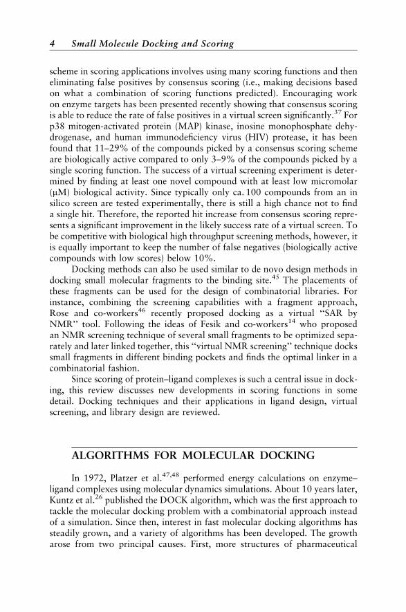
scheme in scoring applications involves using many scoring functions and theneliminating false positives by consensus scoring (i.e., making decisions basedon what a combination of scoring functions predicted). Encouraging workon enzyme targets has been presented recently showing that consensus scoringis able to reduce the rate of false positives in a virtual screen significantly.37 Forp38 mitogen-activated protein (MAP) kinase, inosine monophosphate dehy-drogenase, and human immunodeficiency virus (HIV) protease, it has beenfound that 11–29% of the compounds picked by a consensus scoring schemeare biologically active compared to only 3–9% of the compounds picked by asingle scoring function. The success of a virtual screening experiment is deter-mined by finding at least one novel compound with at least low micromolar(mM) biological activity. Since typically only ca. 100 compounds from an insilico screen are tested experimentally, there is still a high chance not to finda single hit. Therefore, the reported hit increase from consensus scoring repre-sents a significant improvement in the likely success rate of a virtual screen. Tobe competitive with biological high throughput screening methods, however, itis equally important to keep the number of false negatives (biologically activecompounds with low scores) below 10%.

Docking methods can also be used similar to de novo design methods indocking small molecular fragments to the binding site.45 The placements ofthese fragments can be used for the design of combinatorial libraries. Forinstance, combining the screening capabilities with a fragment approach,Rose and co-workers46 recently proposed docking as a virtual ‘‘SAR byNMR’’ tool. Following the ideas of Fesik and co-workers14 who proposedan NMR screening technique of several small fragments to be optimized sepa-rately and later linked together, this ‘‘virtual NMR screening’’ technique dockssmall fragments in different binding pockets and finds the optimal linker in acombinatorial fashion.

Since scoring of protein–ligand complexes is such a central issue in dock-ing, this review discusses new developments in scoring functions in somedetail. Docking techniques and their applications in ligand design, virtualscreening, and library design are reviewed.

ALGORITHMS FOR MOLECULAR DOCKING

In 1972, Platzer et al.47,48 performed energy calculations on enzyme–ligand complexes using molecular dynamics simulations. About 10 years later,Kuntz et al.26 published the DOCK algorithm, which was the first approach totackle the molecular docking problem with a combinatorial approach insteadof a simulation. Since then, interest in fast molecular docking algorithms hassteadily grown, and a variety of algorithms has been developed. The growtharose from two principal causes. First, more structures of pharmaceutical

4 Small Molecule Docking and Scoring

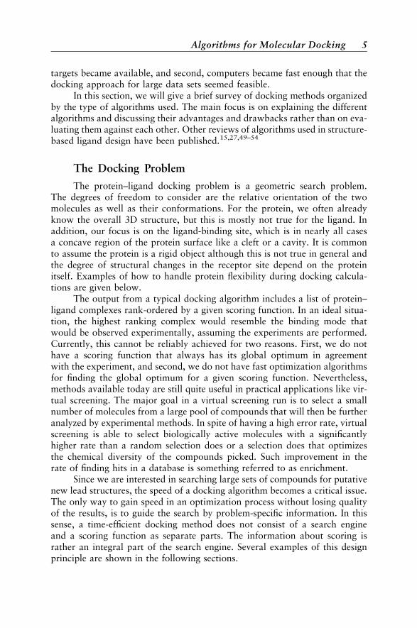
targets became available, and second, computers became fast enough that thedocking approach for large data sets seemed feasible.

In this section, we will give a brief survey of docking methods organizedby the type of algorithms used. The main focus is on explaining the differentalgorithms and discussing their advantages and drawbacks rather than on eva-luating them against each other. Other reviews of algorithms used in structure-based ligand design have been published.15,27,49–54

The Docking Problem

The protein–ligand docking problem is a geometric search problem.The degrees of freedom to consider are the relative orientation of the twomolecules as well as their conformations. For the protein, we often alreadyknow the overall 3D structure, but this is mostly not true for the ligand. Inaddition, our focus is on the ligand-binding site, which is in nearly all casesa concave region of the protein surface like a cleft or a cavity. It is commonto assume the protein is a rigid object although this is not true in general andthe degree of structural changes in the receptor site depend on the proteinitself. Examples of how to handle protein flexibility during docking calcula-tions are given below.

The output from a typical docking algorithm includes a list of protein–ligand complexes rank-ordered by a given scoring function. In an ideal situa-tion, the highest ranking complex would resemble the binding mode thatwould be observed experimentally, assuming the experiments are performed.Currently, this cannot be reliably achieved for two reasons. First, we do nothave a scoring function that always has its global optimum in agreementwith the experiment, and second, we do not have fast optimization algorithmsfor finding the global optimum for a given scoring function. Nevertheless,methods available today are still quite useful in practical applications like vir-tual screening. The major goal in a virtual screening run is to select a smallnumber of molecules from a large pool of compounds that will then be furtheranalyzed by experimental methods. In spite of having a high error rate, virtualscreening is able to select biologically active molecules with a significantlyhigher rate than a random selection does or a selection does that optimizesthe chemical diversity of the compounds picked. Such improvement in therate of finding hits in a database is something referred to as enrichment.

Since we are interested in searching large sets of compounds for putativenew lead structures, the speed of a docking algorithm becomes a critical issue.The only way to gain speed in an optimization process without losing qualityof the results, is to guide the search by problem-specific information. In thissense, a time-efficient docking method does not consist of a search engineand a scoring function as separate parts. The information about scoring israther an integral part of the search engine. Several examples of this designprinciple are shown in the following sections.

Algorithms for Molecular Docking 5

Placing Fragments and Rigid Molecules

The docking problem can be simplified by neglecting the conformationaldegrees of freedom of the ligand molecule. Although this simplification is notappropriate for the general protein–ligand docking scenario, algorithmsbased on this approximation are of great importance and can be applied todocking of small or rigid molecules, molecule fragments, or conformationalensembles of molecules.

Clique-Search Based ApproachesThe docking of two rigid molecules can be understood as a problem of

matching characteristic features of the molecules in space.55 A match is anassignment of a ligand feature to a protein feature. Such a feature can be eithera volume segment of the protein or the ligand or a complementary interactionsuch as a hydrogen-bond donor and acceptor. The search procedure maxi-mizes the number of matches under the constraint that they are compatiblein 3D space, (i.e., that they can be realized simultaneously). Compatibilitymeans that we can find a transformation that simultaneously superimposesall ligand features onto the matched protein features.

To search for compatible matches, a distance compatibility graph isused. The nodes of the graph comprise all possible matches between the pro-tein and the ligand; the edges connect pairs of nodes that are compatible. Com-patibility means mostly distance compatibility within a fixed tolerance e (i.e.,the difference in distance d between the ligand and the protein featuresdiffers by d e). A necessary condition for a set of matches to be simulta-neously formed is that all pairs of matches are distance compatible. Looking atthe distance compatibility graph, a set of matched features is represented by aset of nodes. The distance compatibility between two matched features isrepresented by an edge. Therefore, a set of matched features is distance com-patible exactly, if all pairs of corresponding nodes are connected by an edge.Such a fully connected subgraph is called a clique in graph theory. Searchingfor maximal cliques in graphs is a well-known problem, and although this isa hard optimization problem in theory, fast algorithms exist for practicalapplications.56 We obtain an initial orientation of the ligand molecule in thereceptor site of the protein by superimposing the matched features of a clique(Figure 1).

The algorithm for rigid-body docking in the DOCK program suite26 isbased on the idea of searching for distance-compatible matches. Startingwith the molecular surface of the protein,57–59 a set of spheres is created insidethe receptor site. The spheres represent the volume that could be occupied by aligand molecule (Figure 2). Figure 3 shows an example of the HIV inhibitorVX-478 bound in the active site of the enzyme.60 The ligand is representedeither by spheres inside the ligand or directly by its atoms (Figure 2). In theearly versions of DOCK, an enumeration algorithm searched for sets with

6 Small Molecule Docking and Scoring

up to four distance-compatible matches. Each set was used for an initial fit ofthe ligand into the receptor site. The set was augmented using further compa-tible matches. The position of the ligand was then optimized and scored.

Since its first introduction in 1982, the DOCK software has beenextended in several directions. The matching spheres can be labeled with che-mical properties,61 and distance bins are used to speed up the search pro-cess.62,63 Recently, the search algorithm for distance-compatible matcheswas changed28 to the clique-detection algorithm introduced by Crippen andco-workers.55 Furthermore, several scoring functions are now applied in com-bination with the DOCK algorithm.64–68

Several other approaches such as LUDI,69,70 CLIX,71 and ADAM72 arebased on this clique-search paradigm although somehow differing in the fea-tures used for matching and in the way they are represented.

Geometric Hashing

Geometric hashing73 originated from the area of computer vision andwas first applied to molecular docking problems by Fischer et al.74,75 In com-puter vision, the geometric hashing scheme was developed for the problemof recognizing (partially occluded) objects in camera scenes. In principle,

receptor site ligand

Figure 2 In DOCK, the receptor is geometrically described using overlapping spheres ofdifferent sizes that are complementary to the molecular surface of the ligand-bindingsite. The ligand is described with spheres inside its surface. During the docking processprotein and ligand spheres are matched.

Aa

Ab

DcDbDa

Ca

BcBbBa

A

B

CD

a

b

c

receptor site ligand distance compatibility graph

Cb

CcAc

Figure 1 On the left-hand side, a protein receptor site and a ligand are schematicallydrawn. Some features are highlighted marked by letters. The corresponding distancecompatibility graph is shown on the right. Each distance compatible pair of matchedfeatures is connected by an edge. The three encircled nodes are an example for a clique.

Algorithms for Molecular Docking 7

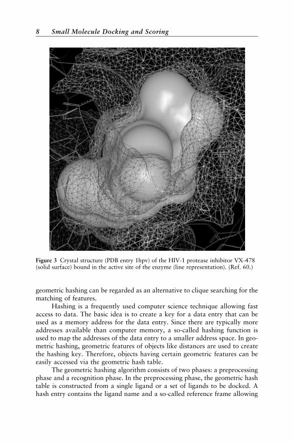
geometric hashing can be regarded as an alternative to clique searching for thematching of features.

Hashing is a frequently used computer science technique allowing fastaccess to data. The basic idea is to create a key for a data entry that can beused as a memory address for the data entry. Since there are typically moreaddresses available than computer memory, a so-called hashing function isused to map the addresses of the data entry to a smaller address space. In geo-metric hashing, geometric features of objects like distances are used to createthe hashing key. Therefore, objects having certain geometric features can beeasily accessed via the geometric hash table.

The geometric hashing algorithm consists of two phases: a preprocessingphase and a recognition phase. In the preprocessing phase, the geometric hashtable is constructed from a single ligand or a set of ligands to be docked. Ahash entry contains the ligand name and a so-called reference frame allowing

Figure 3 Crystal structure (PDB entry 1hpv) of the HIV-1 protease inhibitor VX-478(solid surface) bound in the active site of the enzyme (line representation). (Ref. 60.)

8 Small Molecule Docking and Scoring

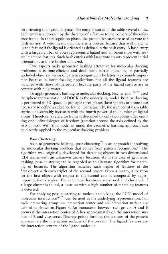
for orienting the ligand in space. The entry is stored in the table several times.Each entry is addressed by the distance of a feature to the corners of the refer-ence frame. In the recognition phase, the protein features are used to vote forhash entries. A vote means that there is a protein feature that will match aligand feature if the ligand is oriented as defined in the hash entry. A hash entrywith a large number of votes represents a ligand and an orientation with sev-eral matched features. Such hash entries with large vote counts represent initialorientations and are further analyzed.

Two aspects make geometric hashing attractive for molecular dockingproblems: it is time-efficient and deals with partial matching or partiallyoccluded objects in terms of pattern recognition. The latter is extremely impor-tant because in most docking applications not all the ligand features arematched with those of the protein because parts of the ligand surface are incontact with bulk water.

To apply geometric hashing to molecular docking, Fischer et al.74,75 usedthe sphere representation of DOCK as the underlying model. Because dockingis performed in 3D space, in principle three points (here spheres or atoms) arenecessary to define a reference frame. Consequently, the number of hash tableentries unacceptably increases with the fourth power of the number of ligandatoms. Therefore, a reference frame is described by only two points after omit-ting one unfixed degree of freedom (rotation around the axis defined by thetwo points). With this model in mind, the geometric hashing approach canbe directly applied to the molecular docking problem.

Pose ClusteringAkin to geometric hashing, pose clustering76 is an approach for solving

the molecular docking problem that comes from pattern recognition.77 Thealgorithm was originally developed for detecting objects in two-dimensional(2D) scenes with an unknown camera location. As in the case of geometrichashing, pose clustering can be regarded as an alternate algorithm for match-ing of features. The algorithm matches each triplet of features of thefirst object with each triplet of the second object. From a match, a locationfor the first object with respect to the second can be computed by super-imposing the triangles. The calculated locations are stored and clustered. Ifa large cluster is found, a location with a high number of matching featuresis detected.

For applying pose clustering to molecular docking, the LUDI model ofmolecular interactions69,70 can be used as the underlying representation. Foreach interacting group, an interaction center and an interaction surface aredefined as shown in Figure 4. An interaction between two groups A and Boccurs if the interaction center of A lies approximately on the interaction sur-face of B and vice versa. Discrete points forming the features of the proteinapproximate the interaction surfaces of the protein. The ligand features arethe interaction centers of the ligand molecule.

Algorithms for Molecular Docking 9

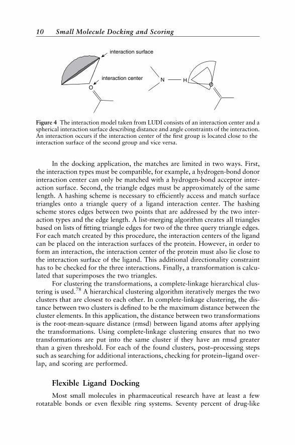
In the docking application, the matches are limited in two ways. First,the interaction types must be compatible, for example, a hydrogen-bond donorinteraction center can only be matched with a hydrogen-bond acceptor inter-action surface. Second, the triangle edges must be approximately of the samelength. A hashing scheme is necessary to efficiently access and match surfacetriangles onto a triangle query of a ligand interaction center. The hashingscheme stores edges between two points that are addressed by the two inter-action types and the edge length. A list-merging algorithm creates all trianglesbased on lists of fitting triangle edges for two of the three query triangle edges.For each match created by this procedure, the interaction centers of the ligandcan be placed on the interaction surfaces of the protein. However, in order toform an interaction, the interaction center of the protein must also lie close tothe interaction surface of the ligand. This additional directionality constrainthas to be checked for the three interactions. Finally, a transformation is calcu-lated that superimposes the two triangles.

For clustering the transformations, a complete-linkage hierarchical clus-tering is used.78 A hierarchical clustering algorithm iteratively merges the twoclusters that are closest to each other. In complete-linkage clustering, the dis-tance between two clusters is defined to be the maximum distance between thecluster elements. In this application, the distance between two transformationsis the root-mean-square distance (rmsd) between ligand atoms after applyingthe transformations. Using complete-linkage clustering ensures that no twotransformations are put into the same cluster if they have an rmsd greaterthan a given threshold. For each of the found clusters, post–processing stepssuch as searching for additional interactions, checking for protein–ligand over-lap, and scoring are performed.

Flexible Ligand Docking

Most small molecules in pharmaceutical research have at least a fewrotatable bonds or even flexible ring systems. Seventy percent of drug-like

O

N

interaction surface

interaction center HO

Figure 4 The interaction model taken from LUDI consists of an interaction center and aspherical interaction surface describing distance and angle constraints of the interaction.An interaction occurs if the interaction center of the first group is located close to theinteraction surface of the second group and vice versa.

10 Small Molecule Docking and Scoring

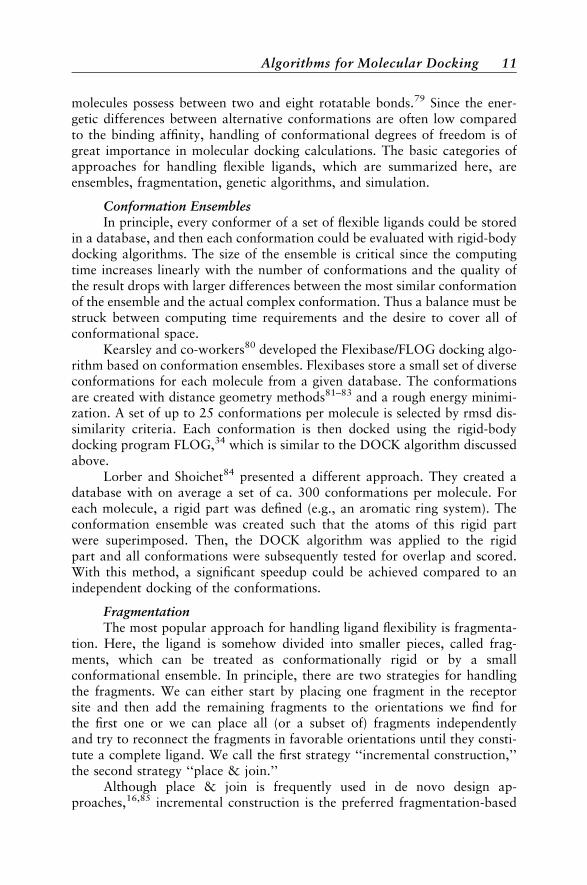
molecules possess between two and eight rotatable bonds.79 Since the ener-getic differences between alternative conformations are often low comparedto the binding affinity, handling of conformational degrees of freedom is ofgreat importance in molecular docking calculations. The basic categories ofapproaches for handling flexible ligands, which are summarized here, areensembles, fragmentation, genetic algorithms, and simulation.

Conformation EnsemblesIn principle, every conformer of a set of flexible ligands could be stored

in a database, and then each conformation could be evaluated with rigid-bodydocking algorithms. The size of the ensemble is critical since the computingtime increases linearly with the number of conformations and the quality ofthe result drops with larger differences between the most similar conformationof the ensemble and the actual complex conformation. Thus a balance must bestruck between computing time requirements and the desire to cover all ofconformational space.

Kearsley and co-workers80 developed the Flexibase/FLOG docking algo-rithm based on conformation ensembles. Flexibases store a small set of diverseconformations for each molecule from a given database. The conformationsare created with distance geometry methods81–83 and a rough energy minimi-zation. A set of up to 25 conformations per molecule is selected by rmsd dis-similarity criteria. Each conformation is then docked using the rigid-bodydocking program FLOG,34 which is similar to the DOCK algorithm discussedabove.

Lorber and Shoichet84 presented a different approach. They created adatabase with on average a set of ca. 300 conformations per molecule. Foreach molecule, a rigid part was defined (e.g., an aromatic ring system). Theconformation ensemble was created such that the atoms of this rigid partwere superimposed. Then, the DOCK algorithm was applied to the rigidpart and all conformations were subsequently tested for overlap and scored.With this method, a significant speedup could be achieved compared to anindependent docking of the conformations.

FragmentationThe most popular approach for handling ligand flexibility is fragmenta-

tion. Here, the ligand is somehow divided into smaller pieces, called frag-ments, which can be treated as conformationally rigid or by a smallconformational ensemble. In principle, there are two strategies for handlingthe fragments. We can either start by placing one fragment in the receptorsite and then add the remaining fragments to the orientations we find forthe first one or we can place all (or a subset of) fragments independentlyand try to reconnect the fragments in favorable orientations until they consti-tute a complete ligand. We call the first strategy ‘‘incremental construction,’’the second strategy ‘‘place & join.’’

Although place & join is frequently used in de novo design ap-proaches,16,85 incremental construction is the preferred fragmentation-based

Algorithms for Molecular Docking 11

strategy for molecular docking. There are several reasons for favoring incre-mental construction. First, if a ligand is divided into fragments, not every frag-ment must lie at a low energy position by itself. Second, consideringthe individual energy contributions, distorting the ligand conformation,especially bond lengths and angles, is very expensive. Therefore, it makessense to directly place fragments such that these distortions do not occur,which can be guaranteed by incremental construction. With place & join,however, a ligand’s bonds are formed after placing the fragments, whichmay result in distorted conformations. A final energy minimization is oftennecessary, which could move the fragments away from their previously calcu-lated favorable positions, thus negating much of the previous placementefforts.

The first place & join algorithm was developed by DesJarlais et al.86 Theligand is manually divided into two fragments having one atom in common.Then, placement lists are created for each fragment using the dockingalgorithm DOCK. The algorithm searches through these lists for placementpairs in which the common atom is located approximately at the same point.Finally, the fragments are reconnected, energy minimized, and scored.

Sandak et al.87–89 applied the geometric hashing paradigm to develop aplace & join algorithm. As before, the ligand is divided into fragments withone overlapping atom, called the hinge. For each ligand atom triplet of a frag-ment, a hash table entry is created addressed with the pairwise distancesbetween the atoms. Each entry contains fragment identification as well asthe location of the hinge. In the matching phase, protein sphere triplets(DOCK spheres) are used to extract ligand atom triplets with similar distances.The method yields a vote for a hinge location for each match. A ‘‘yes’’ vote iscast for the identity of the ligand together with the location and orientation ofthe candidate ligand frame. Hinge locations with high votes are then selected;the fragments are reconnected accordingly and finally scored.

Place & join algorithms are advantageous in cases where the moleculeconsists of a small set of medium-sized rigid fragments. If the fragments aretoo small, it is difficult to place them independently. Another difficulty isthe already mentioned problem of getting correct bond lengths and angles atthe connecting atom without destroying the previously found favorable inter-actions of the fragments to the protein.

Docking algorithms based on incremental construction typically consistof three phases: The selection of a set of so-called base or anchor fragments,the placement of these base fragments, and the incremental construction phaseitself. An incremental construction algorithm can start with several base frag-ments. In contrast to the place & join algorithms, the placements in incremen-tal construction are not combined but taken as an anchoring orientation towhich the remaining parts of the ligand can be added.

Both place & join and incremental construction originated from the areaof de novo ligand design.16,85 Moon and Howe90 created the peptide design

12 Small Molecule Docking and Scoring

tool GROW based on the incremental construction strategy. The first dockingalgorithm based on incremental construction was developed by Leach andKuntz91 based on the DOCK program. In the Leach–Kuntz approach, a singleanchor fragment is first selected manually and docked into the receptor siteusing a variant of the DOCK algorithm, which handles hydrogen-bondingfeatures in the matching phase. A subset of placements is selected favoring ahigh number of matched hydrogen-bond pairs, a high score of the anchorplacement (see the Scoring section), and low similarity to other placements.Subsequently, incremental construction is started for the anchor placementschosen. In this phase, a backtracking algorithm is used that enumerates thespace of nonoverlapping placements of the whole ligand in the receptor site.After adding a fragment to the current placement, a refinement routine is usedto eliminate steric strain and to improve the hydrogen-bonding geometry. Thefinal placements are then filtered, refined, and scored with a force field method.Although there are several manual steps in this procedure, the work demon-strated that the incremental construction idea could be applied to the dockingproblem.

The docking algorithm in the FlexX package is also based on incrementalconstruction.29,92,93 FlexX is a fully automated approach to molecular dock-ing developed for virtual screening purposes. FlexX was the first tool thatdemonstrated computing times short enough for medium-sized screeningefforts with flexible ligand molecular docking.

In the first phase of FlexX’s operation, a small set of base fragments isselected. A simple scoring function is used to select fragments that are suitablefor placement, that is, they contain a reasonably high number of interactinggroups and exhibit a low number of low-energy conformations. A necessarycondition for a successful calculation is that the selected base fragment bindsto the protein and is not mostly exposed to water in the final protein–ligandcomplex. Therefore, it is extremely important to select a set of base fragmentsdistributed over the ligand.

The base fragments are placed with the pose clustering algorithm men-tioned above. Base fragment conformations are enumerated within the place-ment algorithm. The advantage of the pose clustering algorithm is that it isbased on the molecular interactions instead of the shape of the fragment,thus allowing for the handling of much smaller fragments down to the sizeof a single functional group. All calculated placements form the input to theincremental construction phase. In contrast to Leach’s algorithm, a ‘‘greedystrategy’’ is applied that selects a large number k of placements with the high-est estimated scores (typically, k is ca. 800). Each iteration of the incrementalconstruction algorithm contains the following steps: (1) adding the next frag-ment in all possible conformations to all placements from the previous itera-tion (or the base placement phase), (2) searching for new protein–ligandinteractions, (3) optimizing the ligand position to improve the interaction geo-metry and reduce steric strain, (4) selecting a subset of placements with high

Algorithms for Molecular Docking 13

score, and (5) clustering the placements to achieve a reasonable degree ofdiversity in the solution set.

Ligand conformations within FlexX are based on the MIMUMBA mo-del:94 to each rotatable bond, a set of low-energy torsional angles is assigned,previously derived from a statistical analysis of the Cambridge StructuralDatabase (CSD).95 Ring system conformations are precomputed using the3D structure generator CORINA.96,97 For scoring protein–ligand complexes,a variant of Bohm’s empirical scoring function98 is used.

Some extensions of the FlexX approach have been recently developed. Inone publication, the interaction model was extended such that hydrophobicfragments can be handled with the pose clustering algorithm.99 To considerdiscrete water molecules and metal ions located in the protein–ligand inter-face, a technique called the particle concept was invented and integratedinto the FlexX software. The particle concept allows for the automatic place-ment and energetic consideration of approximately spherical objects duringthe docking calculation.100

Two other approaches based on incremental construction have beenpublished. The program Hammerhead32 differs from FlexX in the construc-tion strategy. Instead of adding small fragments (cut between each rotatablebond), the ligand is divided into a small set of large fragments. During the con-struction phase, the next fragment is added such that the connecting atom (orbond) overlaps and interactions to the protein can be formed. There is nodiscrete sampling at the torsional angle of the added fragment. However,high-energy conformations will also be created, and the situation in which afragment does not interact directly with the protein is more difficult to handlethan in FlexX.

Makino and Kuntz101 developed a fully automated incremental con-struction docking algorithm based on backtracking. A single anchor fragmentis selected maximizing hydrogen-bonding features. During the incrementalconstruction phase, the number of conformations for each fragment is limitedto reduce the size of the search space. This method is called a limited backtracksearch. For scoring, the AMBER force field102–104 is used with a modificationthat allows for the handling of multiple protonation states.

Genetic Algorithms and Evolutionary ProgrammingSince 1995, genetic algorithms (GA) are applied to the molecular dock-

ing problem in several approaches.105–109 A genetic algorithm110,111 is a gen-eral purpose optimization scheme that mimics the process of evolution. Theindividuals are configurations in the search space. A so-called fitness functionis used to decide which individuals survive and produce offspring, which arethen used in the next iteration of optimization.

Two aspects of the system must be modeled in order to use the idea ofgenetic algorithms for an application like molecular docking. First, a linearrepresentation of a configuration such as a bit string is needed describing all

14 Small Molecule Docking and Scoring

degrees of freedom of the problem. The linear representation is called a chro-mosome. Finding the chromosome description is the most difficult part ofmodeling. The description should be free of redundancy. If possible, any con-straints of configuration space should be directly modeled such that configura-tions violating constraints are never generated during the optimization.Second, a fitness function has to be developed. The fitness function is closelyrelated to scoring functions for molecular docking with one extension. Scoringfunctions normally work on 3D coordinates. Therefore the chromosome ofan individual has to be interpreted in order to apply the scoring function(genotype-to-phenotype conversion). Since most of the computing time isspent evaluating the fitness function, the conversion and the evaluation haveto be efficient.

The optimization scheme itself is more or less independent of the appli-cation. Typically, several GA parameters such as the population size, the num-ber of generations, crossover, and mutation rates must be chosen.111 It isimportant to find a balance between optimizing the fitness function and main-taining diversity in the population, so that there is a variety of individuals toselect from at each iteration.

Jones et al.21,105 developed one of the first genetic algorithms formolecular docking. Their ideas are implemented in the software tool GOLD.Among the genetic algorithm-based docking approaches, GOLD is probablythe most widely used software. A configuration is represented in GOLD bytwo bit strings. The first string stores the conformation of the ligand (andthe protein) by defining the torsional angle of each rotatable bond. The secondstring stores a mapping between hydrogen-bond partners in the proteinand the ligand. For fitness evaluation, a 3D structure is created from thechromosome representation by first generating the ligand conformation.According to the mapping stored in the second string, hydrogen-bond atomsare superimposed to hydrogen-bond site points in the receptor site. Finally,a scoring function is used as the fitness function for evaluating hydrogenbonds, the ligand internal energy, and the protein–ligand van der Waals (vdw)energy.

Oshiro et al.106 developed two variants of a docking method based on agenetic algorithm and the DOCK approach. The variants differ in the way therelative orientation of the ligand to the protein is described. The first variantencodes the matching of ligand atoms to protein spheres in the chromosome. Asuperposition is used to generate the 3D orientation of the ligand. The secondvariant stores the relative orientation directly by a translation vector and threeEuler angles. For scoring, a simplified version of the AMBER force field102–104

was used as the scoring function.Gehlhaar et al.108,112 developed a docking algorithm called EPDOCK

based on evolutionary programming. In contrast to a genetic algorithm, off-spring are created from one parent by mutation only. Each member of a popu-lation is competing for survival in a kind of a tournament. EPDOCK contains

Algorithms for Molecular Docking 15

its own scoring function based on atomic pair-wise potentials for steric inter-actions and hydrogen bonding.

Molecular SimulationWhereas all previously discussed methods for solving the docking

problem are based on some kind of combinatorial optimization algorithm,there are several approaches for tackling the problem by simulation techni-ques. Instead of trying to enumerate the population of a discrete low-energysubspace of the problem, the simulation approaches begin their calculationwith a starting configuration and move locally to configurations with lowerenergy.

Simulated annealing113 is a well-known simulation technique, which isalso frequently used for solving complex optimization problems without anyphysical interpretation of the simulation itself. The overall simulation routineiterates the following steps. (1) Starting with a configuration A with an energyor score value EðAÞ, we calculate a random local move to a new configurationB with energy EðBÞ. (2) The acceptance of the new configuration is based onthe Metropolis criterion; namely, the configuration is accepted if its energy islower or with probability P¼ exp ð½EðBÞ EðAÞ=½kBTÞ if its energy ishigher. Here kB is the Boltzmann constant, and T is the current absolute tem-perature. During the simulation, T is reduced based on a so-called coolingschedule such that accepting configurations with increased energy becomesless likely over time. The AutoDOCK program for protein–ligand dockingdeveloped by Goodsell and co-workers33,114,115 is based on this strategy.For energy calculation, molecular affinity potentials116 are precalculated ona grid. Yue117 developed a program for optimizing distance constraints forrigid-body docking based on simulated annealing.

Molecular Dynamics Molecular docking problems can in principle besolved with molecular dynamics (MD) simulations. This methodology is quitegeneral because various energy models can be used to simulate the process ofmolecular recognition. However, since the method is following a path from astarting orientation to low-energy configurations, the simulation process canbe quite time consuming. In addition, several simulations with different start-ing orientations must be performed to get a statistically significant result. Thusfar, no MD based technique exists for handling really large data sets in a rea-sonable time frame. However, the methodology is of value for analyzing smallsets of ligands.

In MD, a force field is used to calculate the forces on each atom of thesimulated system. Then, following Newtonian mechanics, velocities and accel-erations are calculated, and the atoms are slightly moved with respect to agiven time step. Introducing molecular dynamics and force fields is clearlybeyond the scope of this chapter, so we refer the reader to earlier reviews inthis book series.118–123 However, some aspects of docking based on MD simu-lations should be briefly mentioned.

16 Small Molecule Docking and Scoring

To avoid very long computing times, scientists look for methods to makegreater moves of the ligand in a single step. Larger steps decrease the depen-dency of the outcome of the docking simulation from the starting structureand allow for a better sampling of the search space. A good examplefor such a method is the ‘‘helicopter view’’ developed by DiNola and co-workers.124,125 For a limited time at the beginning of the simulation, thetemperature of the system is increased for some degrees of freedom (protein–ligand relative orientation) and the repulsive terms of the energy function aredecreased. This increases the amount of structural changes between two simu-lation steps and makes it easier for the system to escape from local minima.

Given and Gilson126 developed a four-phase docking protocol based onMD simulation. First, a set of low-energy ligand conformations is createdusing MD with alternating heating (to perturb the structure) and cooling (tominimize the structure). Then the ligand is several times randomly placed intothe receptor site and minimized. In the final phase, the most stable configura-tions are further investigated using MD with more alternating heating andcooling. The goal of the last phase is to explore the search space around thestable conformations in more detail.

Monte Carlo Algorithms In an MD simulation, the local movement ofthe atoms is performed due to the forces present at each step. In contrast, ina Monte Carlo (MC) simulation, the local moves of the atoms are performedrandomly.

Two components are of major importance in an MC algorithm: thedescription of the degrees of freedom and the energy evaluation. The degreesof freedom should ideally be described such that high-energy states areavoided. Describing the ligand flexibility by internal coordinates (bond angles,torsional angles) can be an advantage compared to a description by 3D coor-dinates in Cartesian space because the force field and MC moves are alsocoded in internal coordinates. The most time-consuming part of an MC simu-lation is the energy (score) calculation. This step must be as time efficient aspossible. Often, energy potentials are precalculated on a grid to speed up thisstep. There are several examples for MC-based docking algorithms. Hart andRead127 developed a combined scheme of MC with simulated annealing. Inthe MC run, random orientations are created and moved such that theprotein–ligand overlap is reduced. The results are then optimized using a simu-lated annealing scheme. Protein–ligand overlap and scores are calculatedbased on precalculated grids. McMartin and Bohacek’s128 QXP program isa similar approach and can be applied to molecular docking and structuralsuperposition. Wallqvist and Covell129 also use MC for optimizing the finalligand orientation. Instead of a random set of starting structures, a surfacematching algorithm is used to align the ligand to a complementary region ofthe protein.

The ICM (Internal Coordinate Mechanics) software package developedby Abagyan et al.130 combines MC as the optimization scheme with an internal

Algorithms for Molecular Docking 17

coordinate description. In contrast to other approaches that make purely ran-dom moves, ICM is able to model probability functions for variable sets. Thisability allows for biasing the MC calculation toward low-energy states.

Apostolakis et al.131 developed a multistep docking protocol based onMC combined with energy minimization. After a random creation of startingstructures, a minimization is performed using a modified van der Waals poten-tial. The energy function for evaluating the conformations is a sum of threeterms: a force field energy, a hydrophobic solvation term that is proportionalto the solvent accessible surface (SAS) of the complex, and an electrostatic sol-vation term obtained from the solution of the linearized Poisson–Boltzmannequation.132 The highest scoring configurations are further analyzed with aMonte Carlo simulation method called MCM that performs Monte Carlomoves interleaved with energy minimization steps.

PRODOCK is an MC-based docking algorithm developed by Trossetand Scheraga.133–135 The software allows use of either the AMBER 4.0 orthe ECEPP/3 force field with a grid-based energy evaluation. For calculatingenergy values within the grid, Bezier splines were used136 allowing for amore accurate estimation of the energy value as well as providing informationabout the derivatives at this point. Like ICM, an internal description of thedegrees of freedom is used. The MC simulation is interleaved with energyminimization steps like in the Apostolakis’ approach.

Alternative MethodsThere is a large variety of methods for molecular docking that do not fit

into one of the most popular algorithmic classes mentioned above. Althoughonly some of them are more widely used today, they form a rich set of com-putational methodologies, which can be used for all kinds of subproblemsoccurring in structure-based ligand design.

Distance Geometry Distance geometry is a well-known technique fromthe area of structure determination via NMR technology.137,138 Instead ofdescribing a molecule by coordinates in Euclidean space, it is described by aso-called distance matrix containing all interatomic distances in the molecule.Based on distance matrices, a set of allowable conformations can be describedin a comprehensive form from a distance interval for each atom pair.

The distance geometry methodology can be directly used in dockingalgorithms based on clique search and distance compatibility as discussedabove. Matches between protein site points and ligand atoms are compatible,if the site point distance lies within the distance interval of the ligand atompair. The drawback of this approach is that the distance matrix is overdeter-mined, that is, for most distance matrices there is more than one set of Carte-sian coordinates of the atoms that satisfy the distance criteria. If matches areformed, the distances between the matched ligand atoms are fixed to the dis-tance of the matched features in the protein. Fixing the atom–atom distancebetween a given atom pair to a single value usually causes other distance

18 Small Molecule Docking and Scoring

intervals to shrink. New upper and lower bounds for distances can then beapproximated exploiting the triangle and tetrangle inequalities.139,140 Never-theless, a very limited number of distance matrices can be converted back to3D space. Examples for methods based on distance geometry have beenreported.141–143

Random Search Most random search approaches involve Monte Carloalgorithms already discussed above. However, there are exceptions in dockingalgorithms that we would like to address here. If a scoring function for eval-uating protein–ligand complexes is available, random search algorithms canbe applied to the docking problem. Random placements can be created eitherindependent of each other (Markov chain) or from a (random) starting struc-ture by subsequent random moves (somewhat mimicking MD simulations). Inmost cases, the structure generation is combined with a numerical optimiza-tion method that drives the placements of the ligand to the closest local mi-nima as done in LIGIN.144

Baxter et al.145 use tabu search as the underlying method of their dockingsoftware called PRO_LEADS. Tabu search starts with an initial random struc-ture; new structures are created by random moves. During the optimizationiterations, a list (the tabu list) is maintained containing the best and mostrecently visited configurations. Moves resulting in configurations close toone in the tabu list are rejected except if they are better than the best scoringone. The tabu list technique improves the sampling properties of the randomsearch algorithm by avoiding revisitation of previously sampled configurations.

Hybrid Methods Due to the complexity of the docking problem, allmethods have their pros and cons. No one method will work well for everyproblem. Combining different methods is therefore a reasonable approach,which can result in methods containing the best of each.

Two recently published methods combine rapid fragment-based search-ing techniques with sophisticated MD or MC simulations. Wang et al.146

developed a multistep approach based on rigid-body docking and MD. First,a set of low-energy conformers is created. Each conformer is docked rigidlyinto the receptor site using DOCK. The high scoring placements are then opti-mized using an MD-based simulated annealing optimization in combinationwith the AMBER force field. Hoffmann et al.147 combined the incrementalconstruction algorithm in FlexX with an MD-based procedure for postoptimi-zation. FlexX is first used to create a sample of a few hundred ligand place-ments. The goal of the second phase is to improve the overall ranking of thesolutions and to identify the correct placement. The placements are energyminimized using the CHARMm22 force field.148,149 The first phase yields alarge number of plausible ligand conformations. Reranking using the softwarepackage CAMLab150 prioritizes those conformations. The final score consistsof three contributions, a force field energy, an electrostatic part of the solva-tion energy, and a nonpolar part of the solvation energy. The electrostatic partof the solvation energy is calculated by solving the Poisson equation using fast

Algorithms for Molecular Docking 19

multigrid methods; the nonpolar part is approximated by the total solventaccessible surface of the protein–ligand complex.

Handling Protein Flexibility

Most approaches for protein–ligand docking treat the protein as a rigidstructure. Although this is an oversimplification in the general case, for manyproteins this is a reasonable assumption, but for other proteins the assumptionfails. Protein flexibility plays an important role in protein–ligand binding,and algorithms considering these additional degrees of freedom should workbetter.

In principle, protein flexibility can directly be handled by MD- or MC-based algorithms as described above. A method to improve time efficiency dur-ing the MD simulation with a flexible protein was developed by Wassermanand co-workers.151,152 In their work, the protein is divided into rigid and flex-ible parts. Every atom, sufficiently far away from the receptor site, is consid-ered as fixed in space; all energy contributions from these atoms can beprecalculated on a grid. During the MD simulation, only the protein’s receptorsite atoms and the ligand atoms are allowed to move and are considered expli-citly in the energy calculation. The method can be combined with an implicitmodel of solvation.

Although such approaches lead to a significant speedup over methodsthat treat the protein as fully flexible, they are still too time consuming forscreening purposes. Therefore, one is interested in introducing protein flexibil-ity into the much faster, fragmentation-based approaches.

To accomplish this, Leach153 developed a docking algorithm similar toincremental construction such that the degrees of freedom are fixed sequen-tially. Degrees of freedom considered in Leach’s method are a discrete set ofligand orientation and conformation as well as a set of rotamers for selectedprotein side chains. To search efficiently through the space of possible config-urations, Leach used a variant of a branch & bound scheme, called A*-algorithm with dead-end elimination (DEE). The A*-algorithm154 is a searchtree algorithm that involves the expansion of nodes. It is capable of finding theoptimal (least cost) path to the global energy minimum of an energy functionfor the assignment of side chain conformations. The DEE154 algorithm on theother hand identifies rotamers of side chains that are incompatible with theglobal minimum energy structure by satisfying the inequality

Eir;rigid þX

j

minðsÞeir;js > Eit ;rigid þX

j

maxðsÞeit ;js ½1

where Eir;rigid is the interaction energy between rotamer r of residue i and thebackbone, eir;js is the interaction energy of rotamer r of residue i and rotamer sof residue j, and min(s)eir;js and max(s)eit ;js are determined by screening all

20 Small Molecule Docking and Scoring

other rotamers that are currently permitted. To address the problem that thetrue global energy minimum of the protein–ligand complex does not necessa-rily correspond to that of the force field, Leach applied a modified DEE/A*algorithm in which an energy threshold is introduced that allows all structureswithin a certain energy difference to the global minimum to satisfy Eq. [1].The large number of possible structures that survive Eq. [1] then defines thespace searched by the A* algorithm.

Knegtel et al.155 extended the DOCK algorithm so that it could handlepartial protein flexibility. Instead of using a single protein 3D structure asinput, an ensemble of protein structures is used for the docking calculation.During the precalculation of scoring grids, all protein structures are used atthe same time such that the grid represents an average structure. In this aver-aging process, the repulsive part of the van der Waals term is neglected forflexible parts of the protein. The advantage of this method is its speed and sim-plicity resulting from the fact that the combinatorics of the protein structure isavoided. This is, of course, a very rough way of approximating protein flex-ibility, especially for the protein–ligand overlap estimation.

The screening software SPECITOPE, developed by Schnecke et al.156,uses distance matrix comparisons as a first filter step. However, flexibility ofmolecules is not modeled by distance intervals. Instead, a weighting scheme isdefined to scale down the contributions of more flexible atom pairs in theoverall score. In addition, a special optimizer is added that allows the removalof protein–ligand steric clashes after the placement calculation.

Recently, Claussen et al.157 presented a new algorithm based on the ideaof protein structure ensembles implemented in the program FlexE. The algo-rithm considers the alternative protein conformations in a truly combinatorialway by calculating the highest scoring protein conformation for each partiallyplaced ligand during an incremental construction algorithm. The new methodis applied to a series of protein ensembles with known ligands. It can be shownthat FlexE successfully docks sets of ligands into proteins where protein flex-ibility is required.

Docking of Combinatorial Libraries

The development of combinatorial chemistry and its application to drugdesign39,40 has had a dramatic impact not only on experimental screeningmethods but also on virtual screening. Due to the increasing number of mole-cules that can be theoretically synthesized, the demand for the throughput ofexperimental and virtual screening systems increased. For real-world pharma-ceutical research, this development led to high-throughput screening basedmostly on a miniaturization of the equipment and parallel processing.

For virtual screening, the situation is somewhat different. Screening canbe understood as a search process for finding the best lead structures availablein a database. Search problems typically become easier to solve if the search

Algorithms for Molecular Docking 21

space is structured. If we search the shortest path to go between two places, wewould never try all possible paths and measure their lengths since we alreadyknow that most paths will not be the shortest due to the structure of the searchspace, which can be expressed, for example, by the triangle inequality. In vir-tual screening, hypothetical combinatorial chemistry can be used to introducestructure into a search space. Combinatorial libraries arise systematically try-ing all combinations of a limited set of building blocks. The resulting databasespace of the enumerated combinatorial library becomes structured by the com-bination pattern of the enumeration scheme. The structuring of the databasecan be exploited to reduce the runtime of virtual screening calculations.

In the context of combinatorial libraries, we distinguish between threekinds of docking problems:

1. Combinatorial Docking Problem: Given a library of ligands, calculate thedocking score (and the geometry of the complex) for each molecule of thelibrary.

2. R-Group Selection Problem: Given a library, select molecules for theindividual R-groups in order to form a smaller sublibrary with an enrichednumber of hits for the target protein.

3. De novo Library Design Problem: Given a catalog of available reagents,design a library (including the rules of synthesis) that will optimize thenumber of hits for the target protein.

Methods for treating these problems have emerged from the area of moleculardocking and de novo ligand design (see, e.g., Kubinyi158 for an overview oncombinatorial docking methods).

Early algorithms for the combinatorial docking problem analyzed thesimilarity among the members of a given ligand data set to speed up the searchprocess. One approach was to generate a minimal tree structure representingthe whole ligand data set.159 Another approach is to speed up conformationalsearching based on clustering similar molecules.160 In both cases, the derivedhierarchy of molecules can be used in an incremental construction dockingmethod.

Recent combinatorial docking tools such as PRO_SELECT161 and Com-biDOCK162 are based on the incremental construction method. In both, alibrary is formed by a template (or core) molecule with a set of attachmentpoints at which a predefined set of substituents can be connected. The templateis then positioned in the receptor site without considering the substituents.Starting from a few orientations of the template, the substituents are attachedto the template independently and the fit to the receptor is assessed. In caseof PRO_SELECT, substituents are selected based on a score (see next sectionfor an introduction to the scoring concept) and additional criteria such as 2Dsimilarity to other substituents and feasibility of synthesis. CombiDOCKcalculates a score for enumerated library molecules by combining fragmentscores.

22 Small Molecule Docking and Scoring

A new algorithm for the combinatorial docking problem based on theFlexX incremental construction algorithm was reported recently.163 The algo-rithm is part of a new combinatorial docking extension of FlexX calledFlexXc. FlexXc considers the combinatorial library as a tree structure. Eachnode represents either the core or an R-group of the library. Molecules fromthe library, required during the docking calculations, are created on the fly.Therefore, the library is handled in its so-called closed form, enumeratingthe library molecules in advance is not necessary. With this method, librarieswith a few hundred thousand molecules can be handled in main memory dur-ing a docking calculation. The tree representation allows the handling of com-plex libraries consisting of several R-groups, that can be arbitrarily linked.One exception is that no ring closures over different R-groups are allowed.A recursive combinatorial library extends the incremental construction me-thod to multiple molecules; in each incremental construction step, all possibleR-group molecules are added sequentially.

Some studies based on ligand de novo design software have been pub-lished for R-group selection problems. Kick et al.164 applied a variant of theBUILDER program165 to the preselection of substituents for a library targetedto cathepsin D. Recently, Bohm applied the LUDI69,166 program to the dockingof two groups of fragments that can be connected pairwise in a single-stepreaction to search for new thrombin inhibitors.167 In principle, all programsfor fragment-based de novo ligand design can be applied in a similar way tothe R-group selection problem.

Finally, we mention two methods for de novo library design. Caflisch168

applied the MCSS169 technique generating fragment placements, which aresubsequently connected. The DREAMþþ software combines tools for frag-ment placement and selection.170 The selection process is done such that onlya small set of well-characterized organic reactions is needed to create thelibrary.

SCORING

The binding affinity between a protein and a ligand that form a non-covalent complex can be experimentally determined, for example, by micro-calorimetry171 or surface plasmon resonance.172 The affinity depends onseveral environmental parameters such as pH and ionic strength of the sol-vent.173 Experimental errors typically lie in the range of 0.1–0.25 kcal/mol,although repeated assays of the same compound can give even wider variabil-ity in some biological systems. Even assuming there exist good experimentaldata for calibrating a computer determination of binding free energies, makingreliable predictions is a very challenging task that has been pursued for dec-ades.174 The binding free energy of a protein–ligand complex can be intuitivelyunderstood as the difference in how much the ligand likes to be in the protein

Scoring 23

binding pocket and how much it likes to be in the solvent (usually aqueoussolution) at infinite separation from the protein. Although there have beenarguments against it,175 the binding free energy is usually dissected into amanifold of ensemble-averaged terms that are sometimes hard to calculate,for example, solvation energies of the ligand, the protein, and the complexðGlig

solv;Gprotsolv ;Gcomplex

solv Þ, interaction energy between the protein and theligand in the complex (Gint), entropy changes for the ligand and the protein(TS), conformational changes (reorganization energy) in ligand and protein(l) upon complex formation. The binding free energy can then be written as

Gbind ¼ Gcomplexsolv Gprot

solv Gprotsolv þGint TS þl ½2

Disregarding the fact that there is no unique set of terms in which the bindingenergy must be expressed, it is key to calculate all the terms and not an arbi-trary subset.176 One problem is that large energy contributions have to bebalanced in order to estimate small binding free energies,177,178 a calculationprone to large statistical and systematic errors.179,180 A second problem arisesfrom the fact that some contributions such as entropy can only be crudelyestimated.181,182 A third problem is that binding free energies can only be rig-orously calculated by fully sampling the conformational space available to theligand in the protein-binding pocket. Algorithms such as free energy perturba-tion179 or the linear response approximation,183,184 which are employed tofacilitate the sampling/free energy calculation task, are too time consumingto be used in docking a large set of ligands. The fast estimation of bindingfree energies requires many simplifications in the model. Simple functionsthat are designed to rank protein–ligand complexes according to their bindingaffinities are therefore referred to as scoring functions rather than energy func-tions. Scoring functions used in docking studies have been reviewedrecently.35,38,174,185 Here, we briefly summarize older techniques and discussnew developments such as knowledge-based scoring functions and consensusscoring.

Scoring functions are the Achilles’ heel of docking algorithms. They canbe divided into several categories. Scoring functions derived from a force fielduse nonbonded interaction terms as the score,21,102,103,186 sometimes in com-bination with solvation terms.67,187 Empirical scoring functions employ multi-variate regression methods to fit coefficients of physically motivated structuralfunctions by using a training set of protein–ligand complexes with measuredbinding constants.69,98,188–193 Knowledge-based scoring functions use statisti-cal atom pair potentials derived from structural databases as the score.194–200

In addition, more heuristic scoring schemes112 such as chemical scores, contactscores, or shape complementary scores are also used.37,62,201–205 The fact thatthe well-established docking programs do not all use the same scoring functionunderlines that no optimal scoring function has yet been found. In fact, noscoring function has been developed so far that reliably and consistently

24 Small Molecule Docking and Scoring

identifies the correct binding mode of a protein–ligand complex.206 Scoringfunctions are usually designed and tested to identify binding modes of knownligands that bind to a well-resolved protein with high affinity. In thoroughlyvalidated docking studies, about 70% of known protein–ligand complexescan usually be reproduced correctly by flexible docking methods.21,29

Shape and Chemical Complementary Scores

Hydrophilic and hydrophobic surface complementarity are often usedfor scoring. Bohacek and McMartin divided the Lee and Richards207 accessibleprotein surface into three separate zones representing hydrophobic, hydrogen-bond donating, or H-bond accepting properties. For nine thermolysin–inhibitor complexes, a correlation between complementary contacts andbinding affinity with an r2 of 0.99 could be achieved. Gehlhaar et al.112 defineda piecewise linear potential (PLP) function used for protein–ligand interac-tions. The potential combines hydrogen-bond donor, hydrogen-bond acceptor,both donor and acceptor, and nonpolar atom types to steric or hydrogen-bondinteractions. The parameters for this simple and very fast scoring scheme wereoptimized employing docking experiments on dihydrofolate reductase(DHFR), FK506-binding protein, and HIV-1 protease. Consequently, thecrystal structures represent the global minima of the PLP scoring function.Intraligand interactions were treated using nonbonded force field terms anda torsional potential term.

Shape and chemical complementarity are also accounted for in DOCKwhere atomic contact potentials for the receptor can be used to construct acubic lattice that fills the volume of the binding site.62 A point on the latticereceives a score of one for every atom within a certain distance and highlynegative scores for any contact that is too close. Polar and apolar contactscan be distinguished. A ligand is scored mapping its atoms onto the nearestlattice points and summing up over all mapped points. Chemical matching(chemical scoring) can be applied in DOCK by ‘‘coloring’’ the DOCK sphereswith respect to the properties of the nearby receptor atoms.55,209 During thesampling process, a sphere can only be matched with a ligand atom of com-plementary color. Chemical color labels can decipher properties such as‘‘H-bond donor,’’ ‘‘H-bond acceptor,’’ ‘‘hydrophobe,’’ ‘‘electronegative,’’‘‘neutral,’’ and so on. These colors are not predefined in DOCK but have tobe assigned by hand.

Walls and Sternberg210 considered surface complementary for dockingprotein–protein complexes using a vdW-like soft core potential. The use ofaccessible surface area on binding and complexation has been discussed, forexample, by Flower.205 Surface descriptors have been used to calculate solva-tion energies as part of the energetics of molecular association.144,188,211

Volume overlap was also used to quantify interactions of chemicalcompounds.201 The HINT exponential function and empirical atomic

Scoring 25

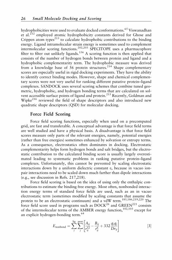
hydrophobicities were used to evaluate docked conformations.65 Viswanadhanet al.212 employed atomic hydrophobicity constants derived for Ghose andCrippen atom types213 to calculate hydrophobic contributions to the bindingenergy. Ligand intramolecular strain energy is sometimes used to complementintermolecular scoring functions.202,203 SPECITOPE uses a pharmacophorefilter to filter out unlikely ligands.156 A scoring function is then applied thatconsists of the number of hydrogen bonds between protein and ligand and ahydrophobic complementarity term. The hydrophobic measure was derivedfrom a knowledge base of 56 protein structures.214 Shape complementaryscores are especially useful in rigid docking experiments. They have the abilityto identify correct binding modes. However, shape and chemical complemen-tary scores were not very useful for ranking different putative protein–ligandcomplexes. SANDOCK uses several scoring schemes that combine tuned geo-metric, hydrophobic, and hydrogen bonding terms that are calculated on sol-vent accessible surface points of ligand and protein.215 Recently, Goldman andWipke216 reviewed the field of shape descriptors and also introduced newquadratic shape descriptors (QSD) for molecular docking.

Force Field Scoring

Force field scoring functions, especially when used on a precomputedgrid, are fast and transferable. A conceptual advantage is that force field termsare well studied and have a physical basis. A disadvantage is that force fieldscores measure only parts of the relevant energies, namely, potential energies(rather than free energies) sometimes enhanced by solvation or entropy terms.As a consequence, electrostatics often dominates in docking. Electrostaticcomplementarity helps form hydrogen bonds and salt bridges, but the electro-static contribution to the calculated binding score is usually largely overesti-mated leading to systematic problems in ranking putative protein–ligandcomplexes. Unfortunately, this cannot be prevented by scaling electrostaticinteractions down by a uniform dielectric constant e, because in vacuo ion-pair interactions need to be scaled down much farther than dipole interactions(e.g., see discussion in Refs. 217,218).

Force field scoring is based on the idea of using only the enthalpic con-tributions to estimate the binding free energy. Most often, nonbonded interac-tion energy terms of standard force fields are used, such as an in vacuoelectrostatic term (sometimes modified by scaling constants that assume theprotein to be an electrostatic continuum) and a vdW term.185,186,219,220 Theforce field score used in programs such as DOCK26 and GREEN221 consistsof the intermolecular terms of the AMBER energy function,102,103 except foran explicit hydrogen-bonding term.64

Enonbond ¼Xlig

i

Xprot

j

Aij

r12ij

Bij

r6ij

þ 332qiqj

Drij

" #½3

26 Small Molecule Docking and Scoring

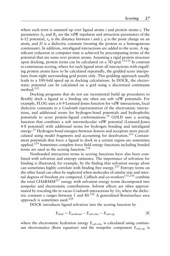
where each term is summed up over ligand atoms i and protein atoms j. Theparameters Aij and Bij are the vdW repulsion and attraction parameters of the6-12 potential, rij is the distance between i and j, q is the point charge on anatom, and D is a dielectric constant (treating the protein as a homogeneouscontinuum). In addition, intraligand interactions are added to the score. A sig-nificant reduction in computer time is achieved by precomputing terms of thepotential that are sums over protein atoms. Assuming a rigid protein structureupon docking, protein terms can be calculated on a 3D grid.33,116 In contrastto continuous scoring, where for each ligand atom all interactions with engulf-ing protein atoms have to be calculated repeatedly, the gridded score interpo-lates from eight surrounding grid points only. This gridding approach usuallyleads to a 100-fold speed up in docking calculations. In DOCK, the electro-static potential can be calculated on a grid using a discretized continuummethod.222

Docking programs that do not use incremental build up procedures toflexibly dock a ligand in a binding site often use soft vdW potentials. Forexample, FLOG uses a 6-9 Lennard-Jones function for vdW interactions, localdielectric constants in a Coulomb representation of the electrostatic interac-tions, and additional terms for hydrogen-bond potentials and hydrophobicpotentials to score protein–ligand conformations.34 GOLD uses a scoringfunction that combines a soft intermolecular vdW potential (Lennard-Jones4-8 potential) with additional terms for hydrogen bonding and intraligandenergy.21 Hydrogen-bond energies between donors and acceptors were precal-culated using model fragments and accounting for desolvation.223 Contain-ment potentials that force a ligand to dock in a certain region are sometimesapplied.224 Sometimes complete force field energy functions including bondedterms are used as the scoring function.134

Nonbonded interaction terms in scoring functions have also been com-bined with solvation and entropy estimates. The importance of solvation forbinding is illustrated, for example, by the finding that solvation energy alonecan sometimes highly correlate with binding free energy.225 Entropy terms onthe other hand can often be neglected when molecules of similar size and inter-nal degrees of freedom are compared. Caflisch and co-workers131,226 combinethe total CHARMM227 energy with solvation energy terms decomposed intononpolar and electrostatic contributions. Solvent effects are often approxi-mated by rescaling the in vacuo Coulomb interactions by 1/e, where the dielec-tric constant e ranges between 1 and 80.126 A generalized Born/surface areaapproach is sometimes used.228

DOCK introduces ligand solvation into the scoring function by

Ebind ¼ Enonbond Esolv;elec Esolv;np ½4

where the electrostatic hydration energy Esolv;elec is calculated using continu-um electrostatics (Born equation) and the nonpolar component Esolv;np is

Scoring 27

calculated based on the surface area of the ligand in the solvent.67 The changein solvation free energy upon protein–ligand binding may also be accountedfor by atomic solvation parameters.211,229,230 Force field terms used in scoringfunctions depend on several parameters such as dielectric constants, non-bonded cutoff schemes, scaling of surface charges, and modification of vdWrepulsion. An analysis of these parameters using the CHARMM energy func-tion was given recently by Vieth et al.231 It was concluded that a soft-core vdWpotential is needed for the kinetic accessibility of the binding site.

Empirical Scoring Functions

The need for fast ranking of protein–ligand complexes led to the designof empirical scoring functions. They use multivariate regression methods thatfit coefficients of physically motivated contributions to the binding free en-ergy to reproduce measured binding affinities of a training set of known 3Dprotein–ligand complexes.98,188–192 Horton and Lewis188 developed anempirical scoring function for protein–protein interaction using polar and apo-lar surface area as well as an entropy term as descriptors. The empirical scor-ing function for protein–ligand complexes designed by Bohm98,189 is probablythe most prominent one. It was originally developed for the de novo designprogram LUDI69 and later used (slightly modified) in the docking programFlexX.29 The free energy of binding for a protein–ligand complex is estimatedin FlexX as the sum of free energy contributions from the number of rotatablebonds in the ligand, hydrogen bonds, ion-pair interactions, hydrophobic andp-stacking interactions of aromatic groups, and lipophilic interactions:

G ¼ G0 þGrotNrot þGhb

Xneutral Hbonds

f ðR;aÞ

þGio

Xionic int

f ðR;aÞ þGaro

Xaro int

f ðR;aÞ

þGlipo

Xlipo:cont

f ðRÞ ½5

where G0;Grot; Ghb; Gio; Garo, and Glipo are adjustable para-meters that were fitted. The parameter f ðR;aÞ is a scaling function pena-lizing deviations from the ideal geometry, and Nrot is the number of freelyrotatable bonds. The interaction of aromatic groups (aro_int term) is an addi-tion to Bohm’s original force field design.98,189 The lipophilic contributions(lipo.cont) are calculated as a sum of atom pair contacts in contrast to evalu-ating a surface grid as in Bohm’s scoring function. Bohm’s scoring functionand its FlexX implementation were being improved and additional termswere being tested (see, e.g., Refs. 31,189). Bohm’s scoring function is some-what sensitive to the orientation and conformation of the ligand in the bindingpocket.

28 Small Molecule Docking and Scoring

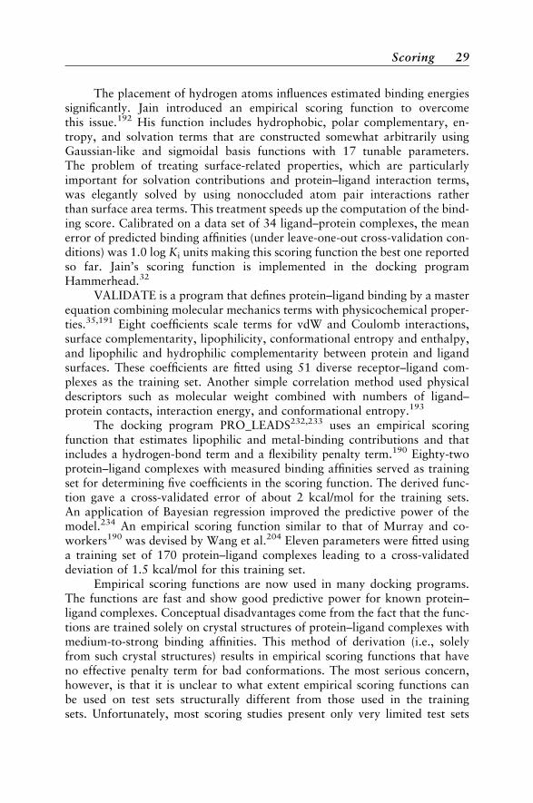
The placement of hydrogen atoms influences estimated binding energiessignificantly. Jain introduced an empirical scoring function to overcomethis issue.192 His function includes hydrophobic, polar complementary, en-tropy, and solvation terms that are constructed somewhat arbitrarily usingGaussian-like and sigmoidal basis functions with 17 tunable parameters.The problem of treating surface-related properties, which are particularlyimportant for solvation contributions and protein–ligand interaction terms,was elegantly solved by using nonoccluded atom pair interactions ratherthan surface area terms. This treatment speeds up the computation of the bind-ing score. Calibrated on a data set of 34 ligand–protein complexes, the meanerror of predicted binding affinities (under leave-one-out cross-validation con-ditions) was 1.0 log Ki units making this scoring function the best one reportedso far. Jain’s scoring function is implemented in the docking programHammerhead.32

VALIDATE is a program that defines protein–ligand binding by a masterequation combining molecular mechanics terms with physicochemical proper-ties.35,191 Eight coefficients scale terms for vdW and Coulomb interactions,surface complementarity, lipophilicity, conformational entropy and enthalpy,and lipophilic and hydrophilic complementarity between protein and ligandsurfaces. These coefficients are fitted using 51 diverse receptor–ligand com-plexes as the training set. Another simple correlation method used physicaldescriptors such as molecular weight combined with numbers of ligand–protein contacts, interaction energy, and conformational entropy.193

The docking program PRO_LEADS232,233 uses an empirical scoringfunction that estimates lipophilic and metal-binding contributions and thatincludes a hydrogen-bond term and a flexibility penalty term.190 Eighty-twoprotein–ligand complexes with measured binding affinities served as trainingset for determining five coefficients in the scoring function. The derived func-tion gave a cross-validated error of about 2 kcal/mol for the training sets.An application of Bayesian regression improved the predictive power of themodel.234 An empirical scoring function similar to that of Murray and co-workers190 was devised by Wang et al.204 Eleven parameters were fitted usinga training set of 170 protein–ligand complexes leading to a cross-validateddeviation of 1.5 kcal/mol for this training set.

Empirical scoring functions are now used in many docking programs.The functions are fast and show good predictive power for known protein–ligand complexes. Conceptual disadvantages come from the fact that the func-tions are trained solely on crystal structures of protein–ligand complexes withmedium-to-strong binding affinities. This method of derivation (i.e., solelyfrom such crystal structures) results in empirical scoring functions that haveno effective penalty term for bad conformations. The most serious concern,however, is that it is unclear to what extent empirical scoring functions canbe used on test sets structurally different from those used in the trainingsets. Unfortunately, most scoring studies present only very limited test sets

Scoring 29

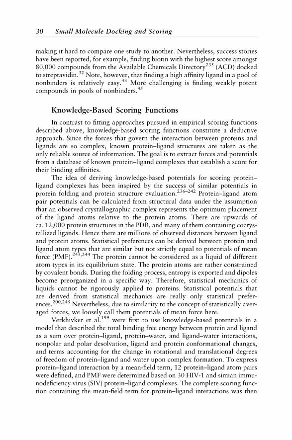
making it hard to compare one study to another. Nevertheless, success storieshave been reported, for example, finding biotin with the highest score amongst80,000 compounds from the Available Chemicals Directory235 (ACD) dockedto streptavidin.32 Note, however, that finding a high affinity ligand in a pool ofnonbinders is relatively easy.43 More challenging is finding weakly potentcompounds in pools of nonbinders.45

Knowledge-Based Scoring Functions

In contrast to fitting approaches pursued in empirical scoring functionsdescribed above, knowledge-based scoring functions constitute a deductiveapproach. Since the forces that govern the interaction between proteins andligands are so complex, known protein–ligand structures are taken as theonly reliable source of information. The goal is to extract forces and potentialsfrom a database of known protein–ligand complexes that establish a score fortheir binding affinities.

The idea of deriving knowledge-based potentials for scoring protein–ligand complexes has been inspired by the success of similar potentials inprotein folding and protein structure evaluation.236–242 Protein–ligand atompair potentials can be calculated from structural data under the assumptionthat an observed crystallographic complex represents the optimum placementof the ligand atoms relative to the protein atoms. There are upwards ofca. 12,000 protein structures in the PDB, and many of them containing cocrys-tallized ligands. Hence there are millions of observed distances between ligandand protein atoms. Statistical preferences can be derived between protein andligand atom types that are similar but not strictly equal to potentials of meanforce (PMF).243,244 The protein cannot be considered as a liquid of differentatom types in its equilibrium state. The protein atoms are rather constrainedby covalent bonds. During the folding process, entropy is exported and dipolesbecome preorganized in a specific way. Therefore, statistical mechanics ofliquids cannot be rigorously applied to proteins. Statistical potentials thatare derived from statistical mechanics are really only statistical prefer-ences.200,245 Nevertheless, due to similarity to the concept of statistically aver-aged forces, we loosely call them potentials of mean force here.

Verkhivker et al.199 were first to use knowledge-based potentials in amodel that described the total binding free energy between protein and ligandas a sum over protein–ligand, protein–water, and ligand–water interactions,nonpolar and polar desolvation, ligand and protein conformational changes,and terms accounting for the change in rotational and translational degreesof freedom of protein–ligand and water upon complex formation. To expressprotein–ligand interaction by a mean-field term, 12 protein–ligand atom pairswere defined, and PMF were determined based on 30 HIV-1 and simian immu-nodeficiency virus (SIV) protein–ligand complexes. The complete scoring func-tion containing the mean-field term for protein–ligand interactions was then

30 Small Molecule Docking and Scoring

successfully applied to reproduce the binding affinities of seven other HIV-1protease complexes. However, the mean-field contribution alone did notshow any correlation with the experimental data.

A preference-based free energy score of enzyme–inhibitor binding wasdeveloped by Wallqvist et al.200 It was applied in docking experiments ofHIV-1 inhibitors.129 Atomic interaction scores between adjacent buried sur-faces of protein and ligand atoms in the binding site were derived by analyzing38 high-resolution protein crystal complexes taken from the PDB. Atom pairpreference scores Pij between protein atoms i and ligand atoms j for 21 atomtypes (10 carbon, 5 oxygen, 5 nitrogen, 1 sulfur atom type) were calculatedand combined with three constants, aij, g, and d to predict protein–ligandbinding affinities,

Gpred ¼ X

i

Xj

aijðgþ d lnPijÞ þ b ½6

This scoring function showed a reliability of 1.5 kcal/mol when tested on eightprotein–ligand complexes.200 The preference-based scoring scheme was usedin docking experiments following a surface complementary screen. It wasfound that 20 rigid enzyme–inhibitor complexes could be reassembled withall-atom root-mean-square deviations of 1.0 A from the native complexes.129

A coarse grained knowledge-based potential was derived by DeWitte andShakhnovich194 as an energy function in the de novo design program SMoG.In the SMoG score, atom pair preferences gij are combined with a simpledistance term ij that is zero if atoms i and j are more than 5 A apart (andone otherwise).

G ¼X

ij

gijij ½7

A more comprehensive mean-field scoring function was reportedrecently.198 Potentials of mean force are derived from a statistical analysisof protein and ligand atom occurrences at certain distances by using 697 pro-tein–ligand complexes taken from the PDB as the knowledge base. Sixteenprotein atom types and 34 ligand atom types are defined and lead to 544PMF interactions of which 282 are statistically significant. The PMF score iscalculated as the sum over all protein–ligand atom pair interaction free ener-gies AijðrÞ as a function of the atom pair distance r by

PMFscore ¼X

kl

r<rij

cutoff

AijðrÞ ½8

where kl is a ligand–protein atom pair of type ij. rijcutoff designates the distance

at which atom pair interactions are truncated. This cutoff distance has been

Scoring 31

found to be optimal at 6 A for carbon–carbon interactions and 9 A otherwise.These values appear to be reasonable given the short-range character of hydro-phobic interactions compared to, e.g., polar interactions. Note, however, thatall AijðrÞ are derived with a reference sphere radius of 12 A. The PMF Aij canbe calculated by

AijðrÞ ¼ kBT ln f jVol corrðrÞ

rijsegðrÞrij

bulk

" #½9

where kB is the Boltzmann factor, T is the absolute temperature, and f jVol corrðrÞ

is a ligand volume correction factor that is introduced because intraligandinteractions are not accounted for.198,246 The parameter rij

segðrÞ designatesthe number density of atom pairs of type ij at a certain atom pair distance r.The parameter rij

bulkðrÞ is the number density of a ligand–protein atom pair oftype ij in a reference sphere with radius R.247 This general and fast scoringfunction was able to reproduce the binding affinities of 77 diverse ligand–protein complexes with a standard deviation of 1.8 log Ki units from measuredbinding affinities. For use in docking studies, the PMF score is combined witha vdW term to account for short-range interactions.45 The PMF scoring func-tion was implemented into the DOCK4.0 program. For faster scoring, it wasalso implemented on a grid similar to the force field score in DOCK. Flexibledocking experiments on FK506 binding protein,45 neuraminidase,20 and stro-melysin248 showed high predictive power and robustness of the PMF score.

Based on sets of 351 and 188 PDB entries, respectively, two mean-fieldfunctions similar to the PMF-score of Muegge and Martin198 (Eqs. [8, 9]) werederived called BLEEP1 and BLEEP2.197 In contrast to BLEEP1, BLEEP2 alsocontains interactions with water. Scoring tests with BLEEP1 and BLEEP2 on90 protein–ligand complexes from the PDB demonstrate a statistically signifi-cant correlation with measured binding constants for BLEEP2 (r2 ¼ 0:55) andsomewhat inferior results for BLEEP1 (r2 ¼ 0:45).249 Standard deviationswere not reported but seem to be on the order of less than 2 log Ki units. Diff-erences between the PMF score (Eq. [8]) and BLEEP are small. They consistmainly of different definitions of atoms types, a different reference state(and reference radius) and a different treatment of intraligand interactions.Recent PMF scoring experiments with the BLEEP test set yielded results com-parable to those of BLEEP1 and BLEEP2.246

Gohlke et al.195 combined a short distance mean-field term (cutoff 6 A)with a solvation term based on solvent accessible surface preferences in aknowledge-based function called DrugScore. DrugScore was used to rankligand placements generated by FlexX for two test sets of 91 and 68protein–ligand complexes from the PDB. It was found that 75% of the bestranking binding modes could be recognized with rmsd of less than 2 A fromthe native binding modes.

32 Small Molecule Docking and Scoring

Knowledge-based scoring functions have the advantage of being moregeneral than empirical scoring functions. The PDB was used as knowledgebase for developing the PMF-score, BLEEP, and DrugScore. Whereas PMF-score and BLEEP use a mean-field term only to score protein–ligand com-plexes, DrugScore and earlier approaches use combinations of mean-fieldterms and extra terms, e.g., for solvation. A recent study of reference statesused in knowledge-based scoring functions was conducted to analyze thedependence of the spherical reference state on the length of its radius. It wasfound that a reference state radius of at least 8 A is needed to implicitlycapture solvation effects in the PMF scoring function.247 The study suggeststhat short-ranged mean-field potentials used in DrugScore or by Verkhivkeret al.199 need additional terms in their models. Knowledge-based scoringfunctions seem to be a promising alternative in docking programs. The fewdocking studies conducted so far with mean-field potential scoring functionsas the primary scoring function (that drives the sampling) suggest that theyare robust and predictive for finding the correct binding mode of a putativeprotein–ligand complex20,248 and for ranking protein–ligand complexesaccording to their binding affinities.45,248

Comparing Scoring Functions in DockingExperiments: Consensus Scoring

As illustrated above, there are plenty of scoring functions availabletoday. Unfortunately, none of them seems to be good enough to be unani-mously adopted by developers of docking programs. Indeed, there are prob-ably no two docking programs that use exactly the same scoring function.To make matters worse, comparison studies of scoring functions are notnumerous and provide conflicting evidence. For instance, Knegtel et al.250 ana-lyzed DOCK with chemical scoring, energy scoring, and FlexX predicting thecorrect binding mode of 32 known thrombin inhibitors by flexible docking.They found that the chemical score outperformed both the energy score andthe FlexX score and identified 10–35% of the native-binding conformationswith rmsd of less than 2 A compared to the crystal coordinates. In contrast,Gohlke et al.195 found that for diverse sets of 91 and 68 protein–ligand com-plexes from the PDB, the DOCK energy score performed similar to the Drug-Score and outperformed the chemical score in identifying correct bindingmodes. Ha et al.248 compared FlexX with energy score and PMF-score inDOCK for 61 biphenyl inhibitors of the matrix metalloproteinase stromelysin(MMP-3). It was found that the PMF score outperformed both the energyscore and the empirical score in FlexX in identifying the correct bindingmode. In fact, the only wrongly predicted binding modes with the DOCK/PMF score were due to sampling insufficiencies rather than scoring problems.Most notably, the PMF score was the only one that found a statistically sig-nificant correlation between predicted score and measured binding affinities of

Scoring 33

the inhibitor–MMP3 complexes. In two other docking studies, one involvingFK506 binding protein45 and the other neuraminidase,20 the superiority ofPMF scoring over energy scoring in DOCK4 was also reported. Stahl251

reported that using PMF scoring in database screening experiments is less sen-sitive to small coordinate changes than is the FlexX score. Finally, a compar-ison for a variety of sets of protein–ligand complexes from the PDB showedthe superiority of PMF scoring over SMoG and Bohm’s score.198

To better discern between active and inactive inhibitors or ligands indocking experiments, more than one scoring function can be used. Sometimestwo different scoring functions are used, one to find the correct binding modeand the other to locally optimize and score the resulting ligand–protein com-plex. For instance, Wallqvist and Covell129 used a surface complementarityscore to find a limited set of binding modes and then invoked a preference-based free energy surface score to quantify the binding affinity. Gohlkeet al.195 used FlexX to generate a limited number of possible binding modesand employed DrugScore as an ‘‘after-score’’ to identify the correct bindingmode. Stahl251 also relied on FlexX to generate protein–ligand conformationsand then evaluated them by using the PMF score. Scoring results can also beimproved by introducing filter functions that remove structures with unfavor-able properties.252

Recently, Charifson et al.37 presented a comprehensive consensus scoringapproach applying two docking approaches and 13 scoring functions. ThisVertex group used the energy scoring function of DOCK as primary scoringfunction along with GAMBLER, a genetic algorithm docker, that employsthe piecewise linear potential112 (PLP) as its primary score. Scoring functionsto after-score the binding modes included empirical scoring functions (Bohm’sscore,69 ChemScore,190,234 SCORE,204 PLP112), force fields (Merck molecularforce field nonbonded energy,253 DOCK energy score,28,64 DOCK chemicalscore, FLOG score,34 strain energy) and some other methods (Poisson-Boltzmann,254 buried lipophilic surface area,205 DOCK contact score,62

volume overlap201). No knowledge-based scoring functions were included.The docking/scoring study involving three different enzymes showed that byusing the intersection of the top scoring compounds of each scoring hit list,significant reductions in the list of false positives in the docking screen couldbe obtained. The confirmed hit rates of weakly active chemical entities (IC50

<50 mM) were between 2 and 7% (IC50 is the concentration of drug requiredto inhibit a biological or biochemical process by 50%). Consensus scoring isa significant improvement over typical hit rates that are on the order of only0–3% in virtual screens. By comparing the different scoring functions andcombinations thereof, it was found that ChemScore, PLP, and DOCK energyscore performed best singly and in consensus.

Simplex minimization during rescoring led to improved docked orienta-tions and scores.63 Finally, it should be mentioned that a consensus scoringspreadsheet is also available in SYBYL,255 which combines four scoring

34 Small Molecule Docking and Scoring

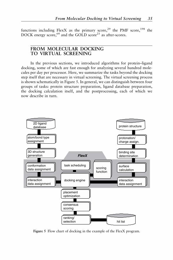
functions including FlexX as the primary score,29 the PMF score,198 theDOCK energy score,64 and the GOLD score21 as after-scores.

FROM MOLECULAR DOCKINGTO VIRTUAL SCREENING

In the previous sections, we introduced algorithms for protein–liganddocking, some of which are fast enough for analyzing several hundred mole-cules per day per processor. Here, we summarize the tasks beyond the dockingstep itself that are necessary in virtual screening. The virtual screening processis shown schematically in Figure 5. In general, we can distinguish between fourgroups of tasks: protein structure preparation, ligand database preparation,the docking calculation itself, and the postprocessing, each of which wenow describe in turn.

2D liganddatabase

atom/bond typeassignment

3D structuregeneration

conformationdata assignment

interactiondata assignment

task scheduling

docking engine

placementoptimization

consensusscoring

ranking/selection

scoringfunction

protein structure

protonation/charge assign.

binding sitedetermination

surfacecalculation

interactiondata assignment

hit list

FlexX

Figure 5 Flow chart of docking in the example of the FlexX program.

From Molecular Docking to Virtual Screening 35

Protein Data Preparation

Preparing a protein 3D structure is usually the same for single dockingcalculations as for virtual screening. Typical steps are the calculation of pro-tonation states and the assignment of atomic charges. The receptor site has tobe determined, which is a critical step because a too small receptor site limitsthe available search space, whereas a larger receptor site costs more computingtime. Although algorithms for receptor site determination are available (e.g.,LIGSITE256), it is generally a good idea to invest time in the manual selectionof the binding site because automated methods often fail.206 Other steps some-times necessary for docking are the determination of the protein surface atomsand the assignment of interaction data such as chemical coloring of atoms andsite points. Whether these steps are necessary depends on the docking soft-ware; these steps are internally included in some programs (e.g., in theprogram FlexX) but have to be done separately in others (e.g., in DOCK).

Ligand Database Preparation

Since we often have to consider several thousand small molecules in aligand database, manual steps in data preparation must be avoided. Typically,information on available ligands is stored in 2D form (atom types and connec-tivity) in MDL databases257 that frequently serve as data repositories for thepharmaceutical industry. Starting from a database of 2D structures, atom andbond types must first be checked and corrected; protonation states and chargeshave to be assigned. This procedure is typically done with rule-based formattranslation programs such as db_translate.255 Next, 3D structures have tobe created for the database using programs such as CORINA258 orCONCORD.259 Finally, physicochemical data necessary for calculating ligandconformations (e.g., rotational barriers or allowed side-chain rotamers) aswell as protein–ligand interactions (e.g., site points that guarantee properhydrogen-bonding directionality) have to be assigned. Within FlexX, theassignment of physicochemical data is done automatically via a set of so-calledstatic data files containing this information on the basis of subgraphs thatcould flexibly be matched to the ligand molecule. For example, FlexX containsthe MIMUMBA torsional angle database,94 which contains information aboutfrequently occurring torsional angles for small molecules determined for abouta thousand different molecular fragments.

Docking Calculation

The docking calculations are usually iterated separately for each mole-cule of a database. Since the calculation times per molecule are still quite largeeven for fast algorithms (about a minute per ligand), the use of a workstationcluster or parallel hardware is of great advantage. Within FlexX, a task

36 Small Molecule Docking and Scoring

scheduler is employed that distributes docking processes on heterogeneousworkstation clusters based on the Parallel Virtual Machine260 (PVM) soft-ware. The scheduler automatically detects whether a parallel-processing envir-onment is available and starts docking processes on a user defined subset of theavailable computers. The scheduler is very flexible allowing, for example, userinitiated interruptions of the calculation, handling of partial and total failureof the computing environment, and recovery of interrupted calculations. Inaddition, the scheduler contains an automatic output file merging procedure,which is able to handle the output of several hundred docking processes run-ning in parallel. For the user, the whole process is transparent, that is, theresulting output files are identical for calculations performed on a single pro-cessor and those performed on a 1024-processor parallel computer. Of course,in the latter case the result is calculated about a thousand-fold faster.

Postprocessing

After the docking calculation, a set of placements and a score are calcu-lated for most of the database compounds. The failure rate of compounds thatcannot be placed in the receptor site at all depends on the size of the com-pounds in the database and on the thresholds set for the maximum scores orthe minimum matched features such as DOCK spheres. Typically, the numberof unplaced compounds in a database is below 5%. The score can then be usedto create an initial ranking of the compounds. Several postprocessing steps canbe invoked including the optimization of placements with numerical techni-ques such as MD or the filtering of placements not fulfilling additional con-straints that were omitted by the primary scoring function.252 Due to thewell-known limitations of individual scoring functions, it can be helpful toapply alternative scoring schemes such as the consensus scoring already dis-cussed. If a set of inhibitors with known bioactivity is contained in the data-base, their docking results can be used to customize the scoring and to estimatehow far in rank one should consider molecules for biological testing.

APPLICATIONS

Docking as a Virtual Screening Tool

Biological screening methods are commonly used for lead identificationin a drug discovery program. High throughput screening (HTS) is usuallyemployed to experimentally screen hundreds of thousands of compoundsagainst a drug target.41 Molecular databases can be extended via combinator-ial chemistry39,40 or compound acquisition. Today, proprietary databasesoften contain about 106 compounds. However, this is only a tiny fractionof the conceivable molecular space for which estimates range between 1060

Applications 37

and 10100 compounds.43,44 Computational screening methods can comple-ment HTS because they are fast, cheap, and applicable to even virtual com-pounds. The calculations can help in deciding which compounds out of thevast pool of possibilities should be made in a combinatorial or medicinalchemistry program. The realm of virtual screening includes techniques thatevaluate the drug-likeness261 of compounds, development parameters,262

and the 2D and 3D diversity263,264 of designed libraries.43,44,265 Virtualscreening can even evaluate compound libraries based on the compounds’potential for favorable characteristics in regard to absorption, distribution,metabolism, excretion, and toxicity (ADME / TOX). Here, we want to com-ment on the role docking plays as usually the last filter in library designs.

Automated docking is often used to rank a library of putative ligand–protein complexes according to their binding affinities. One of the main pro-blems in virtual screening is the large number of false positives, that is, inactivecompounds that nevertheless have high scores (bioactive compounds with lowscores are called false negatives). To illustrate the problem, we quote Jain192

who gives the following example: ‘‘Suppose that in a database of 100,000compounds just 20 will bind above some threshold affinity to the target inquestion. Even if the false negative rate is high (say 50%) one would likelybe happy with finding 10 true hits. However, depending on how many com-pounds may be practically obtained (through purchase or synthesis) andassayed, the false positive rate has a significant impact on the likelihood offinding the true hits. If the false positive rate is just 1%, there will be 1000 falsepositive ‘hits’ in the screen. If there is the capacity to obtain and assay 50 of the1010 hits, with no principled way of distinguishing true positives from falsepositives, there is a 60% chance of not finding a single true hit. In order toachieve a 90% chance of finding at least one true hit, the absolute false posi-tive rate must be 0.2%.’’

Fortunately, many virtual screening test studies can identify highlypotent, known inhibitors32 or derivatives thereof101 when seeded in large data-bases of nonbinders. However, more realistic applications of virtual screeninginclude the identification of novel micromolar lead structures from a chemicaldatabase—a task that is much harder to accomplish due to the small differencein binding affinities between active and inactive compounds. (It should bepointed out by way of comparison that actual compound databases used atmost large pharmaceutical companies easily give many micromolar hits forsome target receptors, but few or none for other receptors.)

Early examples of academically successful identification of potentiallead compounds by virtual screening with DOCK include drug targets suchas HIV-1 protease, RNase H, thymidylate synthase, hemagglutinin, andmalaria protease.27 Shoichet et al.61 discovered a new class of thymidylatesynthase inhibitors by screening the Available Chemicals Directory (ACD)and also identified a binding mode different from that of the natural substrate.Grootenhuis et al.266 identified a potent antitumor agent by virtually screening

38 Small Molecule Docking and Scoring

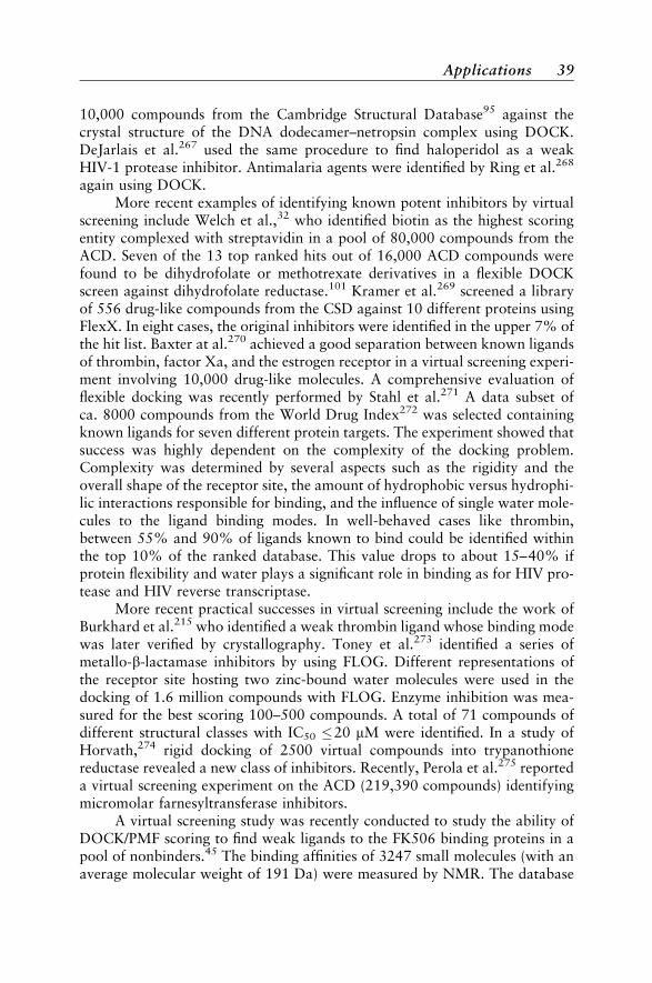
10,000 compounds from the Cambridge Structural Database95 against thecrystal structure of the DNA dodecamer–netropsin complex using DOCK.DeJarlais et al.267 used the same procedure to find haloperidol as a weakHIV-1 protease inhibitor. Antimalaria agents were identified by Ring et al.268

again using DOCK.More recent examples of identifying known potent inhibitors by virtual

screening include Welch et al.,32 who identified biotin as the highest scoringentity complexed with streptavidin in a pool of 80,000 compounds from theACD. Seven of the 13 top ranked hits out of 16,000 ACD compounds werefound to be dihydrofolate or methotrexate derivatives in a flexible DOCKscreen against dihydrofolate reductase.101 Kramer et al.269 screened a libraryof 556 drug-like compounds from the CSD against 10 different proteins usingFlexX. In eight cases, the original inhibitors were identified in the upper 7% ofthe hit list. Baxter at al.270 achieved a good separation between known ligandsof thrombin, factor Xa, and the estrogen receptor in a virtual screening experi-ment involving 10,000 drug-like molecules. A comprehensive evaluation offlexible docking was recently performed by Stahl et al.271 A data subset ofca. 8000 compounds from the World Drug Index272 was selected containingknown ligands for seven different protein targets. The experiment showed thatsuccess was highly dependent on the complexity of the docking problem.Complexity was determined by several aspects such as the rigidity and theoverall shape of the receptor site, the amount of hydrophobic versus hydrophi-lic interactions responsible for binding, and the influence of single water mole-cules to the ligand binding modes. In well-behaved cases like thrombin,between 55% and 90% of ligands known to bind could be identified withinthe top 10% of the ranked database. This value drops to about 15–40% ifprotein flexibility and water plays a significant role in binding as for HIV pro-tease and HIV reverse transcriptase.

More recent practical successes in virtual screening include the work ofBurkhard et al.215 who identified a weak thrombin ligand whose binding modewas later verified by crystallography. Toney et al.273 identified a series ofmetallo-b-lactamase inhibitors by using FLOG. Different representations ofthe receptor site hosting two zinc-bound water molecules were used in thedocking of 1.6 million compounds with FLOG. Enzyme inhibition was mea-sured for the best scoring 100–500 compounds. A total of 71 compounds ofdifferent structural classes with IC50 20 mM were identified. In a study ofHorvath,274 rigid docking of 2500 virtual compounds into trypanothionereductase revealed a new class of inhibitors. Recently, Perola et al.275 reporteda virtual screening experiment on the ACD (219,390 compounds) identifyingmicromolar farnesyltransferase inhibitors.

A virtual screening study was recently conducted to study the ability ofDOCK/PMF scoring to find weak ligands to the FK506 binding proteins in apool of nonbinders.45 The binding affinities of 3247 small molecules (with anaverage molecular weight of 191 Da) were measured by NMR. The database

Applications 39

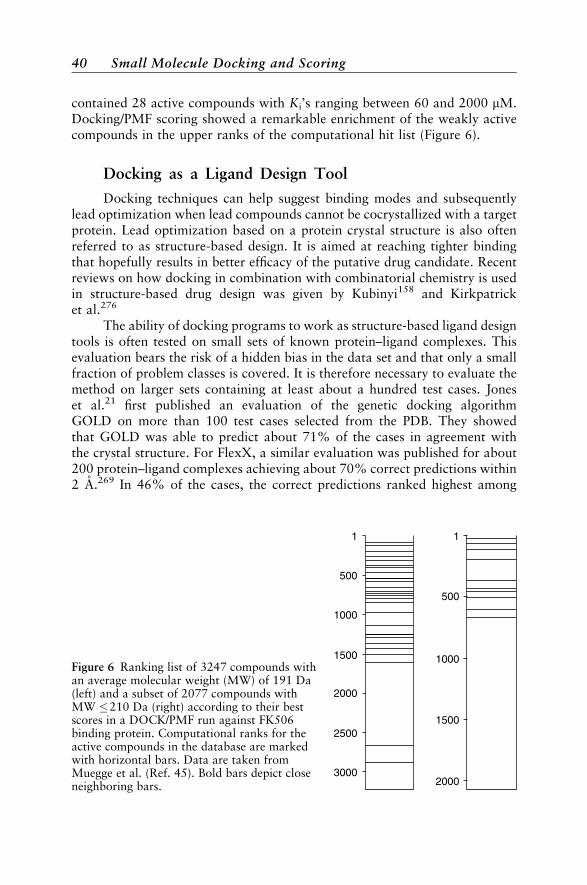
contained 28 active compounds with Ki’s ranging between 60 and 2000 mM.Docking/PMF scoring showed a remarkable enrichment of the weakly activecompounds in the upper ranks of the computational hit list (Figure 6).

Docking as a Ligand Design Tool

Docking techniques can help suggest binding modes and subsequentlylead optimization when lead compounds cannot be cocrystallized with a targetprotein. Lead optimization based on a protein crystal structure is also oftenreferred to as structure-based design. It is aimed at reaching tighter bindingthat hopefully results in better efficacy of the putative drug candidate. Recentreviews on how docking in combination with combinatorial chemistry is usedin structure-based drug design was given by Kubinyi158 and Kirkpatricket al.276

The ability of docking programs to work as structure-based ligand designtools is often tested on small sets of known protein–ligand complexes. Thisevaluation bears the risk of a hidden bias in the data set and that only a smallfraction of problem classes is covered. It is therefore necessary to evaluate themethod on larger sets containing at least about a hundred test cases. Joneset al.21 first published an evaluation of the genetic docking algorithmGOLD on more than 100 test cases selected from the PDB. They showedthat GOLD was able to predict about 71% of the cases in agreement withthe crystal structure. For FlexX, a similar evaluation was published for about200 protein–ligand complexes achieving about 70% correct predictions within2 A.269 In 46% of the cases, the correct predictions ranked highest among

3000

2500

2000

1000

1500

500

1

2000

1000

1500

500

1

Figure 6 Ranking list of 3247 compounds withan average molecular weight (MW) of 191 Da(left) and a subset of 2077 compounds withMW 210 Da (right) according to their bestscores in a DOCK/PMF run against FK506binding protein. Computational ranks for theactive compounds in the database are markedwith horizontal bars. Data are taken fromMuegge et al. (Ref. 45). Bold bars depict closeneighboring bars.

40 Small Molecule Docking and Scoring

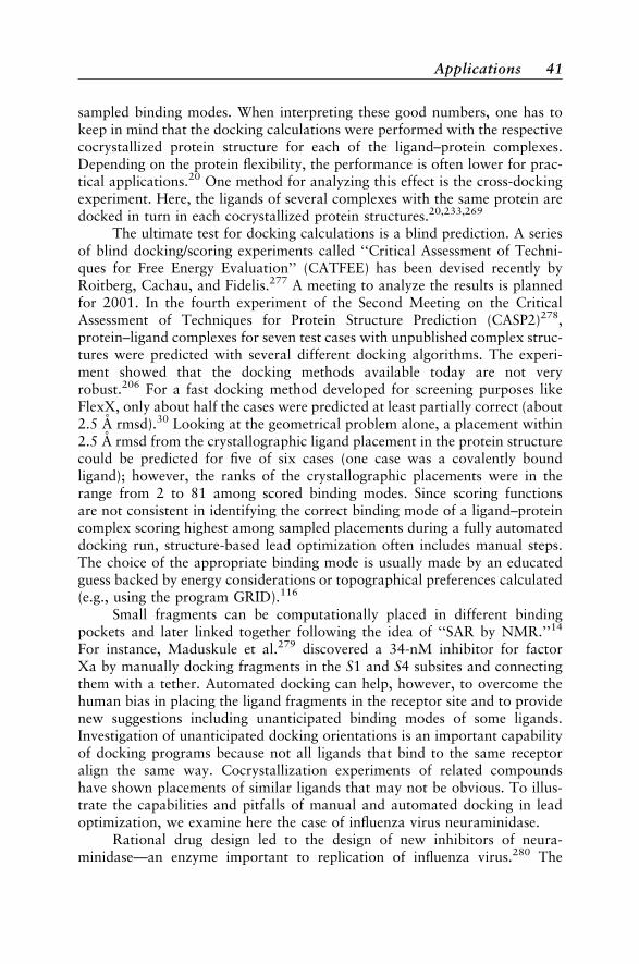
sampled binding modes. When interpreting these good numbers, one has tokeep in mind that the docking calculations were performed with the respectivecocrystallized protein structure for each of the ligand–protein complexes.Depending on the protein flexibility, the performance is often lower for prac-tical applications.20 One method for analyzing this effect is the cross-dockingexperiment. Here, the ligands of several complexes with the same protein aredocked in turn in each cocrystallized protein structures.20,233,269

The ultimate test for docking calculations is a blind prediction. A seriesof blind docking/scoring experiments called ‘‘Critical Assessment of Techni-ques for Free Energy Evaluation’’ (CATFEE) has been devised recently byRoitberg, Cachau, and Fidelis.277 A meeting to analyze the results is plannedfor 2001. In the fourth experiment of the Second Meeting on the CriticalAssessment of Techniques for Protein Structure Prediction (CASP2)278,protein–ligand complexes for seven test cases with unpublished complex struc-tures were predicted with several different docking algorithms. The experi-ment showed that the docking methods available today are not veryrobust.206 For a fast docking method developed for screening purposes likeFlexX, only about half the cases were predicted at least partially correct (about2.5 A rmsd).30 Looking at the geometrical problem alone, a placement within2.5 A rmsd from the crystallographic ligand placement in the protein structurecould be predicted for five of six cases (one case was a covalently boundligand); however, the ranks of the crystallographic placements were in therange from 2 to 81 among scored binding modes. Since scoring functionsare not consistent in identifying the correct binding mode of a ligand–proteincomplex scoring highest among sampled placements during a fully automateddocking run, structure-based lead optimization often includes manual steps.The choice of the appropriate binding mode is usually made by an educatedguess backed by energy considerations or topographical preferences calculated(e.g., using the program GRID).116

Small fragments can be computationally placed in different bindingpockets and later linked together following the idea of ‘‘SAR by NMR.’’14

For instance, Maduskule et al.279 discovered a 34-nM inhibitor for factorXa by manually docking fragments in the S1 and S4 subsites and connectingthem with a tether. Automated docking can help, however, to overcome thehuman bias in placing the ligand fragments in the receptor site and to providenew suggestions including unanticipated binding modes of some ligands.Investigation of unanticipated docking orientations is an important capabilityof docking programs because not all ligands that bind to the same receptoralign the same way. Cocrystallization experiments of related compoundshave shown placements of similar ligands that may not be obvious. To illus-trate the capabilities and pitfalls of manual and automated docking in leadoptimization, we examine here the case of influenza virus neuraminidase.

Rational drug design led to the design of new inhibitors of neura-minidase—an enzyme important to replication of influenza virus.280 The

Applications 41

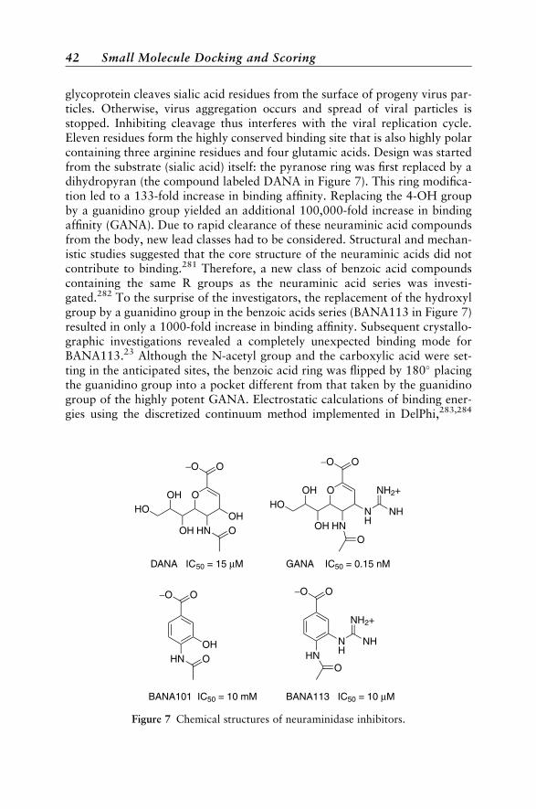
glycoprotein cleaves sialic acid residues from the surface of progeny virus par-ticles. Otherwise, virus aggregation occurs and spread of viral particles isstopped. Inhibiting cleavage thus interferes with the viral replication cycle.Eleven residues form the highly conserved binding site that is also highly polarcontaining three arginine residues and four glutamic acids. Design was startedfrom the substrate (sialic acid) itself: the pyranose ring was first replaced by adihydropyran (the compound labeled DANA in Figure 7). This ring modifica-tion led to a 133-fold increase in binding affinity. Replacing the 4-OH groupby a guanidino group yielded an additional 100,000-fold increase in bindingaffinity (GANA). Due to rapid clearance of these neuraminic acid compoundsfrom the body, new lead classes had to be considered. Structural and mechan-istic studies suggested that the core structure of the neuraminic acids did notcontribute to binding.281 Therefore, a new class of benzoic acid compoundscontaining the same R groups as the neuraminic acid series was investi-gated.282 To the surprise of the investigators, the replacement of the hydroxylgroup by a guanidino group in the benzoic acids series (BANA113 in Figure 7)resulted in only a 1000-fold increase in binding affinity. Subsequent crystallo-graphic investigations revealed a completely unexpected binding mode forBANA113.23 Although the N-acetyl group and the carboxylic acid were set-ting in the anticipated sites, the benzoic acid ring was flipped by 180 placingthe guanidino group into a pocket different from that taken by the guanidinogroup of the highly potent GANA. Electrostatic calculations of binding ener-gies using the discretized continuum method implemented in DelPhi,283,284

O

−O O

OHHN OOH

OHHO

O

−O O

NHHNOH

OHHO

NH

NH2+

−O O

HN OOH N

HHNNH

NH2+

−O O

O

O

DANA IC50 = 15 µM GANA IC50 = 0.15 nM

BANA101 IC50 = 10 mM BANA113 IC50 = 10 µM

Figure 7 Chemical structures of neuraminidase inhibitors.

42 Small Molecule Docking and Scoring

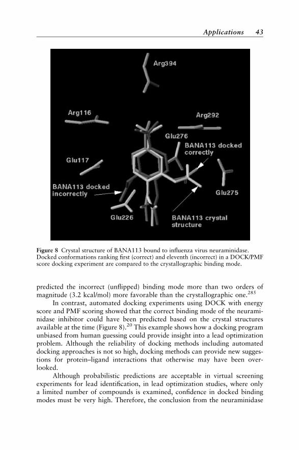
predicted the incorrect (unflipped) binding mode more than two orders ofmagnitude (3.2 kcal/mol) more favorable than the crystallographic one.285

In contrast, automated docking experiments using DOCK with energyscore and PMF scoring showed that the correct binding mode of the neurami-nidase inhibitor could have been predicted based on the crystal structuresavailable at the time (Figure 8).20 This example shows how a docking programunbiased from human guessing could provide insight into a lead optimizationproblem. Although the reliability of docking methods including automateddocking approaches is not so high, docking methods can provide new sugges-tions for protein–ligand interactions that otherwise may have been over-looked.

Although probabilistic predictions are acceptable in virtual screeningexperiments for lead identification, in lead optimization studies, where onlya limited number of compounds is examined, confidence in docked bindingmodes must be very high. Therefore, the conclusion from the neuraminidase

Figure 8 Crystal structure of BANA113 bound to influenza virus neuraminidase.Docked conformations ranking first (correct) and eleventh (incorrect) in a DOCK/PMFscore docking experiment are compared to the crystallographic binding mode.

Applications 43

example is that one should use all techniques available at the time, includingautomated docking, in order to gather ideas about possible protein–ligandinteractions and then examine all the results before making design decisions.This comprehensive strategy is particularly important in light of the fact that itis not uncommon for similar ligands to bind in different binding modes to thesame protein.173

CONCLUDING REMARKS

A wide range of different methods for protein–ligand docking is avail-able today. Although the docking of small and rigid ligands in their boundconformations is often successful, the docking of flexible drug-like ligandsinto a rigid binding site of a protein already presents a problem that is not gen-erally solved. Protein flexibility, solvent molecules, and increasing ligand sizeintroduce additional difficulties. Fast methods for the conformational sam-pling of binding modes of protein–ligand complexes have been developed. Pro-grams typically sample large numbers of different low-energy configurations ina few minutes of computer time. The main challenge of docking programstoday is to recognize the correct binding mode once it is sampled. Scoringfunctions are designed to facilitate this task. They are the actual Achilles’heel of docking programs. Scoring functions are not reliable enough today.However, progress has been made recently in the development of empiricaland knowledge-based scoring functions as well as by the addition of solvationterms into force field scores.

Docking is the essence of in silico (virtual) screening tools. Fast and sim-ple functions are employed that filter compounds out of a database that haveno chance to fit the desired target. This filtering can be done, for example, bypharmacophore-like feature matching in the binding site. For the survivors ofthe initial screening, a more elaborate docking scheme is applied. The relativeranking of different protein–ligand structures according to their binding affi-nities is the crucial problem in a virtual screening application. The scoring pro-blem is even more challenging in ranking protein–ligand complexes than infinding the correct binding mode of a single ligand–protein complex. Typi-cally, scoring results in large numbers of false positives in a virtual screen.False positive rates can be reduced by using several scoring functions in aconsensus-scoring strategy.37 The ultimate goal of virtual screening is to mimicexperimental high throughput screening results. For virtual screening to becompetitive, the ratio between real hits and false positives must be pushedabove 10%. If a database of 106 compounds contains 10 actives, the numberof false positives must be below 100 (i.e., 0.01% of the total database).Although this goal is not reached today, docking as a virtual screening toolcan still be useful in drug design projects. Virtual screening is fast and cheapbecause there is no need to develop a screening assay as well as no need to

44 Small Molecule Docking and Scoring

purchase, synthesize, or store the compounds to be screened. Therefore, vir-tual screening can be beneficial as an initial filter in cases where a full high-throughput screening cannot be conducted, for either technical or cost reasons.On the other hand, virtual screening requires the existence of an appropriate3D structure of the target molecule.

In ligand design, the strength of protein–ligand docking methods liesin the quick creation of a variety of plausible binding modes for a putativeprotein–ligand complex. Computationally proposed binding modes can beof value in suggesting modifications of a lead structure. These suggestionscan then be tested experimentally. Sometimes, unexpected binding modes ofprotein–ligand complexes are predicted that help to solve lead optimizationpuzzles and guide medicinal chemistry efforts in a drug discovery program.

The technical revolution in high-speed chemical synthesis and biologicalhigh throughput screening techniques has somewhat outpaced computationalapproaches in recent years. One could argue that it does not make much senseto elaborately calculate binding affinities for a small number of compounds ifthey can be made and tested experimentally much faster. Therefore, the mainopportunity for docking techniques today is to suggest new compounds thatwould not have been identified in HTS or synthesized as part of an ongoingSAR exploration. The need to generate novel chemical matter for a drug targetis apparent if one looks at the surprisingly low success rate of HTS throughoutthe pharmaceutical industry. Only one in about ten HTS runs produces anacceptable lead that is optimized in a drug discovery program.286 Moreover,for many proteins (e.g., orphan receptors), HTS cannot be developed due tolack of reference compounds. It is now recognized that HTS cannot be thesole source of lead compounds in the pharmaceutical industry. Rational designtechniques, which did not enjoy undivided support in the pharmaceuticalindustry in prior decades, have flourished recently. Small molecule dockinghas contributed much to the recent successes of rational drug design. Todayvirtual screening belongs to the standard repertoire of many pharmaceuticalresearch operations. Some pharmaceutical companies such as Vertex almostexclusively prosecute drug targets for which they can generate crystal struc-tures.287 Virtual screening and docking for lead optimization are used asmain tools. As a result, the average number of compounds made in a drugoptimization program at Vertex is an order of magnitude smaller than at otherpharmaceutical companies. The fact that today only one in about 29,000 smallmolecules synthesized in the pharmaceutical industry results in a profitabledrug288 illustrates the drastic potential that rational drug design can have oncost reduction in the drug discovery.

Current efforts are directed toward improving the reliability of scoringfunctions as well as increased docking speed.289 High throughput crystallogra-phy in combination with fast and reliable docking and scoring algorithmswould cause a revolution in drug design. From our perspective, there arehigh expectations of docking/scoring approaches for the future.

Concluding Remarks 45

ACKNOWLEDGMENTS

We would like to thank the Editors Kenny Lipkowitz and Don Boyd for carefullyediting the manuscript. Also, we would like to thank Thomas Lengauer (GMD) and Martin Stahl(F. Hoffmann-La Roche AG, Basel) for helpful suggestions and discussions.

REFERENCES

1. A. T. Brunger, J. Kuryan, and M. Karplus, Science, 235, 458 (1987). Crystallographic RFactor Refinement by Molecular Dynamics.

2. S. Subbiah, Science, 252, 128 (1991). Low-Resolution Real Space Envelopes: An Approach tothe Ab Initio Macromolecular Phase Problem.

3. W. Kuhlbrandt, Q. Rev. Biophys., 25, 1 (1992). Two-Dimensional Crystallization ofMembrane Proteins.

4. A. T. Brunger, Nature (London), 355, 472 (1992). A Novel Statistical Quantity for Assessingthe Accuracy of Crystal Structures.

5. J. L. Markley, Methods Enzymol., 176, 12 (1989). Two-Dimensional Nuclear MagneticResonance Spectroscopy of Proteins: An Overview.

6. G. M. Clore and A. M. Gronenborn, Science, 252, 1390 (1991). Structures of Larger Proteinsin Solution: Three- and Four-Dimensional Heteronuclear NMR Spectroscopy.

7. S. W. Fesik, J. Med. Chem., 34, 2937 (1991). NMR Studies of Molecular Complexes as a Toolin Drug Design.

8. A. Bax and S. Grzesiek, Acc. Chem. Res., 26, 131 (1993). Methodological Advances in ProteinNMR.

9. F. C. Bernstein, T. F. Koetzle, G. J. B. Williams, E. F. Meyer Jr., M. D. Brice, J. R. Rodgers,O. Kennard, T. Shimanouchi, and M. Tasumi, Eur. J. Biochem., 80, 319 (1977). The ProteinData Bank. A Computer-Based Archival File for Macromolecular Structures.

10. H. M. Berman, J. Westbrook, Z. Feng, G. Gilliland, T. N. Bhat, H. Weissig, I. N. Shindyalov,and P. E. Bourne, Nucleic Acids Res., 28, 235 (2000). The Protein Data Bank.

11. T. P. Hubbard, A. M. Lesk, and A. Tramontano, Nature Struct. Biol., 3, 313 (1996).Gathering Them in to the Fold.

12. URL http://www.rcsb.org/pdb.

13. V. L. Nienaber, P. L. Richardson, V. Klighofer, J. J. Bouska, V. L. Giranda, and J. Greer,Nature Biotech., 18, 1105 (2000). Discovering Novel Ligands for Macromolecules UsingX-Ray Crystallography Screening.

14. S. B. Shuker, P. J. Hajduk, R. P. Meadows, and S. W. Fesik, Science, 274, 1531 (1996).Discovering High-Affinity Ligands for Protein SAR by NMR.

15. J. M. Blaney and J. S. Dixon, Perspect. Drug Disc. Des., 15, 301 (1993). A Good Ligand IsHard to Find: Automatic Docking Methods.

16. M. A. Murcko, in Reviews in Computational Chemistry, K. B. Lipkowitz and D. B. Boyd,Eds., Wiley-VCH, New York, 1997, Vol. 11, pp. 1–66. Recent Advances in Ligand DesignMethods.

17. C. Sander and R. Schneider, Proteins: Struct., Funct., Genet., 9, 56 (1991). Database ofHomology-Derived Protein Structures and the Structural Meaning of Sequence Alignment.

18. T. L. Blundell, B. L. Sibanda, M. J. E. Sternberg, and J. M. Thornton, Nature (London), 326,347 (1987). Knowledge-Based Prediction of Protein Structures and the Design of NovelMolecules.

19. A. Vedani, P. Zbinden, J. P. Snyder, and P. A. Greenidge, J. Am. Chem. Soc., 117, 4987(1995). Pseudoreceptor Modeling: The Construction of Three-Dimensional Receptor Sur-rogates.

46 Small Molecule Docking and Scoring

20. I. Muegge, Med. Chem. Res., 9, 490 (1999). The Effect of Small Changes in Protein Structureon Predicted Binding Modes of Known Inhibitors of Influenza Virus Neuraminidase: PMF-Scoring in DOCK4.

21. G. Jones, P. Willett, R. C. Glen, and A. R. Leach, J. Mol. Biol., 267, 727 (1997). Developmentand Validation of a Genetic Algorithm for Flexible Docking.

22. K. Sekar, S. Eswaramoorthy, M. K. Jain, and M. Sundaralingam, Biochemistry, 36, 14186(1997). Crystal Structure of the Complex of Bovine Pancreatic Phospholipase A2 with theInhibitor 1-Hexadecyl-3-(trifluoroethyl)-sn-glycero-2-phosphomethanol.

23. E. A. Sudbeck, M. J. Jedrzejas, S. Singh, W. J. Brouillette, G. M. Air, W. G. Laver, Y. S. Babu,S. Bantia, P. Chand, N. Chu, J. A. Montgomery, D. A. Walsh, and M. Luo, J. Mol. Biol., 267,584 (1997). Guanidinobenzoic Acid Inhibitors of Influenza Virus Neuraminidase.

24. L. P. Ehrlich and R. C. Wade, in Reviews in Computational Chemistry, K. B. Lipkowitz andD. B. Boyd, Eds., Wiley-VCH, New York, 2001, Vol. 17, pp. 61–97. Protein–Protein Docking.

25. W. L. Jorgensen, Science, 254, 954 (1991). Rusting of the Lock and Key Model for Protein–Ligand Binding.

26. I. D. Kuntz, J. M. Blaney, S. J. Oatley, and R. L. Langridge, J. Mol. Biol., 161, 269 (1982). AGeometric Approach to Macromolecule–Ligand Interactions.

27. I. D. Kuntz, Science, 257, 1078 (1992). Structure-Based Strategies for Drug Design andDiscovery.

28. T. J. A. Ewing and I. D. Kuntz, J. Comput. Chem., 18, 1175 (1997). Critical Evaluation ofSearch Algorithms for Automated Molecular Docking and Database Screening.

29. M. Rarey, B. Kramer, T. Lengauer, and G. Klebe, J. Mol. Biol., 261, 470 (1996). A FastFlexible Docking Method Using an Incremental Construction Algorithm.

30. B. Kramer, M. Rarey, and T. Lengauer, Proteins: Struct., Funct., Genet., 1, 221 (1997).CASP2 Experiences with Docking Flexible Ligands Using FlexX.

31. B. Kramer, G. Metz, M. Rarey, and T. Lengauer, Med. Chem. Res., 9, 463 (1999). LigandDocking and Screening with FlexX.

32. W. Welch, J. Ruppert, and A. N. Jain, Chem. Biol., 3, 449 (1996). Hammerhead—Fast, FullyAutomated Docking of Flexible Ligands to Protein Binding Sites.

33. D. S. Goodsell and A. J. Olson, Proteins: Struct., Funct., Genet., 8, 195 (1990). AutomatedDocking of Substrates to Proteins by Simulated Annealing.

34. M. D. Miller, S. K. Kearsley, D. J. Underwood, and R. P. Sheridan, J. Comput.-Aided Mol.Des., 8, 153 (1994). FLOG: A System to Select Quasi-flexible Ligands Complementary to aReceptor of Known 3-Dimensional Structure.

35. T. I. Oprea and G. R. Marshall, Perspect. Drug Discovery Des., 9/10/11, 35 (1998).Receptor-Based Prediction of Binding Affinities.

36. H. J. Bohm and M. Stahl, Med. Chem. Res., 9, 445 (1999). Rapid Empirical Scoring Functionsin Virtual Screening Applications.

37. P. S. Charifson, J. J. Corkery, M. A. Murcko, and W. P. Walters, J. Med. Chem., 42, 5100(1999). Consensus Scoring: A Method for Obtaining Improved Hit Rates from DockingDatabases of Three-Dimensional Structures into Proteins.

38. J. R. H. Tame, J. Comput.-Aided Mol. Des., 13, 99 (1999). Scoring Functions: A View fromthe Bench.

39. M. A. Gallop, R. W. Barrett, W. J. Dower, S. P. A. Fodor, and A. M. Gordon, J. Med. Chem.,37, 1233 (1994). Applications of Combinatorial Technologies to Drug Discovery. 1.Background and Peptide Combinatorial Libraries.

40. E. M. Gordon, R. W. Barrett, W. J. Dower, S. P. A. Fodor, and M. A. Gallop, J. Med. Chem.,37, 1385 (1994). Applications of Combinatorial Technologies to Drug Discovery 2.Combinatorial Organic Synthesis, Library Screening Strategies, and Future Directions.

41. M. W. Lutz, J. A. Menius, T. D. Choi, R. G. Laskody, P. L. Domanico, A. S. Goetz, and D. L.Saussy, Drug Discovery Today, 1, 277 (1996). Experimental Design for High ThroughputScreening.

References 47

42. R. F. Burns, R. M. A. Simmons, J. J. Howbert, D. C. Waters, P. G. Threlkeld, and B. D. Gitter,in Exploiting Molecular Diversity, Symposium Proceedings, Cambridge Healthtech Insti-tute, San Diego, CA, Vol. 2, p. 6, January 23–25, 1995. Virtual Screening as a Tool forEvaluating Chemical Libraries.

43. W. P. Walters, M. T. Stahl, and M. A. Murcko, Drug Discovery Today, 3, 160 (1998). VirtualScreening—an Overview.

44. Y. C. Martin, Perspect. Drug Discovery Des., 7/8, 159 (1997). Challenges and Prospects forComputational Aids to Molecular Diversity.

45. I. Muegge, Y. C. Martin, P. J. Hajduk, and S. W. Fesik, J. Med. Chem., 42, 2498 (1999).Evaluation of PMF Scoring in Docking Weak Ligands to the FK506 Binding Protein.

46. T. J. Marrone, B. A. Luty, and P. W. Rose, Perspect. Drug Discovery Des., 20, 209 (2000).Discovering High-Affinity Ligands from the Computationally Predicted Structures andAffinities of Small Molecules Bound to a Target: A Virtual Screening Approach.

47. K. E. B. Platzer, F. A. Momany, and H. A. Scheraga, Int. J. Peptide Protein Res., 4, 187(1972). Conformational Energy Calculations of Enzyme–Substrate Interactions. I. Compu-tation of Preferred Conformation of Some Substrates of a-Chymotrypsin.

48. K. E. B. Platzer, F. A. Momany, and H. A. Scheraga, Int. J. Peptide Protein Res., 4, 201(1972). Conformational Energy Calculations of Enzyme–Substrate Interactions. II. Com-putation of the Binding Energy for Substrates in the Active Site of a-Chymotrypsin.

49. W. C. Guida, Curr. Opin. Struct. Biol., 4, 777 (1994). Software for Structure-Based DrugDesign.

50. P. M. Colman, Curr. Opin. Struct. Biol., 4, 868 (1994). Structure-Based Drug Design.

51. T. P. Lybrand, Curr. Opin. Struct. Biol., 5, 224 (1995). Ligand–Protein Docking and RationalDrug Design.

52. R. Rosenfeld, S. Vajda, and C. DeLisi, Ann. Rev. Biophys. Biomol. Struct., 24, 677 (1995).Flexible Docking and Design.

53. H. J. Bohm, Curr. Opin. Biotech., 7, 433 (1996). Current Computational Tools for De NovoLigand Design.

54. T. Lengauer and M. Rarey, Curr. Opin. Struct. Biol., 6, 402 (1996). Computational Methodsfor Biomolecular Docking.

55. F. S. Kuhl, G. M. Crippen, and D. K. Friesen, J. Comput. Chem., 5, 24 (1984). ACombinatorial Algorithm for Calculating Ligand Binding.

56. C. Bron and J. Kerbosch, Commun. Assoc. Computing Machinery, 16, 575 (1973). FindingAll Cliques of an Undirected Graph.

57. F. M. Richards, Ann. Rev. Biophys. Bioeng., 6, 151 (1977). Areas, Volumes, Packing, andProtein Structure.

58. M. L. Connolly, J. Appl. Crystallogr., 16, 548 (1983). Analytical Molecular SurfaceCalculation.

59. M. L. Connolly, J. Appl. Crystallogr., 18, 499 (1985). Molecular Surface Triangulation.

60. E. E. Kim, C. T. Baker, M. D. Dwyer, M. A. Murcko, B. G. Rao, R. D. Tung, and M. A. Navia,J. Am. Chem. Soc., 117, 1181 (1995). Crystal Structure of HIV-1 Protease in Complex withVX-478, A Potent and Orally Bioavailable Inhibitor of the Enzyme.

61. B. K. Shoichet, R. M. Stroud, D. V. Santi, I. D. Kuntz, and K. M. Perry, Science, 259, 1445(1993). Structure-Based Discovery of Inhibitors of Thymidylate Synthase.

62. B. K. Shoichet, D. L. Bodian, and I. D. Kuntz, J. Comput. Chem., 13, 380 (1992). MolecularDocking Using Shape Descriptors.

63. E. C.Meng, D. A.Gschwend, J. M. Blaney, and I.D.Kuntz,Proteins: Struct., Funct., Genet., 17,266 (1993). Orientational Sampling and Rigid-Body Minimization in Molecular Docking.

64. E. C. Meng, B. K. Shoichet, and I. D. Kuntz, J. Comput. Chem., 13, 505 (1992). AutomatedDocking with Grid-Based Energy Evaluation.

48 Small Molecule Docking and Scoring

65. E. C. Meng, I. D. Kuntz, D. J. Abraham, and G. E. Kellogg, J. Comput.-Aided Mol. Des., 8,299 (1994). Evaluating Docked Complexes with the HINT Exponential Function andEmpirical Atomic Hydrophobicities.

66. D. A. Gschwend and I. D. Kuntz, J. Comput.-Aided Mol. Des., 10, 123 (1996). OrientationalSampling and Rigid-Body Minimization in Molecular Docking Revisited—On-the-FlyOptimization and Degeneracy Removal.

67. B. K. Shoichet, A. R. Leach, and I. D. Kuntz, Proteins: Struct., Funct., Genet., 34, 4 (1999).Ligand Solvation in Molecular Docking.

68. X. Q. Zou, Y. X. Sun, and I. D. Kuntz, J. Am. Chem. Soc., 121, 8033 (1999). Inclusion ofSolvation in Ligand Binding Free Energy Calculations Using the Generalized-Born Model.

69. H.-J. Bohm, J. Comput.-Aided Mol. Des., 6, 593 (1992). LUDI: Rule-Based AutomaticDesign of New Substituents for Enzyme Inhibitor Leads.

70. H. Bohm, J. Comput.-Aided Mol. Des., 6, 61 (1992). The Computer Program LUDI: A NewMethod for the De Novo Design of Enzyme Inhibitors.

71. M. C. Lawrence and P. C. Davis, Proteins: Struct., Funct., Genet., 12, 31 (1992). CLIX: ASearch Algorithm for Finding Novel Ligands Capable of Binding Proteins of Known Three-Dimensional Structure.

72. M. Y. Mizutani, N. Tomioka, and A. Itai, J. Mol. Biol., 243, 310 (1994). Rational AutomaticSearch Method for Stable Docking Models of Protein and Ligand.

73. Y. Lamdan and H. J. Wolfson, in Proceedings of the IEEE International Conference onComputer Vision, 1988, pp. 238–249. Geometric Hashing: A General and Efficient Model-Based Recognition Scheme.

74. D. Fischer, R. Norel, H. Wolfson, and R. Nussinov, Proteins: Struct., Funct., Genet., 16, 278(1993). Surface Motifs by a Computer Vision Technique: Searches, Detection and Implica-tions for Protein–Ligand Recognition.

75. D. Fischer, S. L. Lin, H. L. Wolfson, and R. Nussinov, J. Mol. Biol., 248, 459 (1995). AGeometry-Based Suite of Molecular Docking Processes.

76. S. Linnainmaa, D. Harwood, and L. S. Davis, IEEE, Transactions on Pattern Analysis andMachine Intelligence, 10, 634 (1988). Pose Determination of a Three-Dimensional ObjectUsing Triangle Pairs.

77. M. Rarey, S. Wefing, and T. Lengauer, J. Comput.-Aided Mol. Des., 10, 41 (1996). Placementof Medium-Sized Molecular Fragments Into Active Sites of Proteins.

78. R. O. Duda and P. E. Hart, Pattern Classification and Scene Analysis, Wiley, New York,1973.

79. T. I. Oprea, J. Comput.-Aided Mol. Des., 14, 251 (2000). Property Distribution of Drug-Related Chemical Databases.

80. S. K. Kearsley, D. J. Underwood, R. P. Sheridan, and M. D. Miller, J. Comput.-AidedMol. Des., 8, 153 (1994). Flexibases: A Way to Enhance the Use of Molecular DockingMethods.

81. T. F. Havel, I. D. Kuntz, and G. M. Crippen, J. Theoret. Biol., 104, 359 (1983). TheCombinatorial Distance Geometry Approach to the Calculation of Molecular Conforma-tion. 1. A New Approach to an Old Problem.

82. T. F. Havel, I. D. Kuntz, and G. M. Crippen, Bull. Math. Biol., 45, 665 (1983). The Theoryand Practice of Distance Geometry.

83. G. M. Crippen and T. F. Havel, Distance Geometry and Molecular Conformation, ResearchStudies Press, Taunton, UK, 1988.

84. D. M. Lorber and B. K. Shoichet, Protein Sci., 7, 938 (1998). Flexible Ligand Docking UsingConformational Ensembles.

85. D. E. Clark, C. W. Murray, and J. Li, in Reviews in Computational Chemistry, K. B.Lipkowitz and D. B. Boyd, Eds., Wiley-VCH, New York, 1997, Vol. 11, pp. 67–125. CurrentIssues in De Novo Molecular Design.

References 49

86. R. L. DesJarlais, R. P. Sheridan, J. S. Dixon, I. D. Kuntz, and R. Venkataraghavan, J. Med.Chem., 29, 2149 (1986). Docking Flexible Ligands to Macromolecular Receptors byMolecular Shape.

87. B. Sandak, R. Nussinov, and H. J. Wolfson, IEEE Workshop on Shape and Pattern Matchingin Computational Biology, 41 (1994). 3-D Flexible Docking of Molecules.

88. B. Sandak, R. Nussinov, and H. J. Wolfson, Computer Applications in the Biosciences, 11, 87(1995). An Automated Computer Vision and Robotics-Based Technique For 3-D FlexibleBiomolecular Docking and Matching.

89. B. Sandak, R. Nussinov, and H. J. Wolfson, J. Comput. Biol., 5, 631 (1998). A Method forBiomolecular Structural Recognition and Docking Allowing Conformational Flexibility.

90. J. B. Moon and W. J. Howe, Proteins: Struct., Funct., Genet., 11, 314 (1991). ComputerDesign of Bioactive Molecules: A Method for Receptor-Based De Novo Ligand Design.

91. A. R. Leach and I. D. Kuntz, J. Comput. Chem., 13, 730 (1992). Conformational Analysis ofFlexible Ligands in Macromolecular Receptor Sites.

92. M. Rarey, B. Kramer, and T. Lengauer, in Proceedings of the Third International Conferenceon Intelligent Systems in Molecular Biology, C. Rawlings, Ed., AAAI Press, Menlo Park, CA,1995, pp. 300–308. Time-Efficient Docking of Flexible Ligands into Active Sites of Proteins.

93. M. Rarey, B. Kramer, and T. Lengauer, J. Comput.-Aided Mol. Des., 11, 369 (1997). MultipleAutomatic Base Selection—Protein–Ligand Docking Based on Incremental ConstructionWithout Manual Intervention.

94. G. Klebe and T. Mietzner, J. Comput.-Aided Mol. Des., 8, 583 (1994). A Fast and EfficientMethod to Generate Biologically Relevant Conformations.

95. F. H. Allen, S. Bellard, M. D. Brice, B. A. Cartwright, A. Doubleday, H. Higgs, T.Hummelink-Peters, O. Kennard, W. D. S. Motherwell, J. R. Rodgers, and D. G. Watson,Acta Crystallogr., B35, 2331 (1979). The Cambridge Crystallographic Data Center:Computer-Based Search, Retrieval, Analysis and Display of Information.

96. J. Gasteiger, C. Rudolph, and J. Sadowski, Tetrahedron Computer Methodology, 3, 537(1990). Automatic Generation of 3D-Atomic Coordinates for Organic Molecules.

97. J. Sadowski, J. Gasteiger, and G. Klebe, J. Chem. Inf. Comput. Sci., 34, 1000 (1994).Comparison of Automatic Three-Dimensional Model Builders Using 639 X-Ray Structures.

98. H.-J. Bohm, J. Comput.-Aided Mol. Design, 8, 243 (1994). The Development of a SimpleEmpirical Scoring Function to Estimate the Binding Constant for a Protein–Ligand Complexof Known Three–Dimensional Structure.

99. M. Rarey, B. Kramer, and T. Lengauer, Bioinformatics, 15, 243 (1999). Docking ofHydrophobic Ligands with Interaction-Based Matching Algorithms.

100. M. Rarey, B. Kramer, and T. Lengauer, Proteins: Struct., Funct., Genet., 34, 17 (1999).The Particle Concept: Placing Discrete Water Molecules During Protein–Ligand DockingPredictions.

101. S. Makino and I. D. Kuntz, J. Comput. Chem., 18, 1812 (1997). Automated Flexible LigandDocking Method and Its Application for Database Search.

102. S. J. Weiner, P. A. Kollman, D. A. Case, U. C. Singh, C. Ghio, G. Alagona, S. Profeta Jr., andP. Weiner, J. Am. Chem. Soc., 106, 765 (1984). A New Force Field for MolecularMechanical Simulation of Nucleic Acids and Proteins.

103. S. J. Weiner, P. A. Kollman, D. T. Nguyen, and D. A. Case, J. Comput. Chem., 7, 230 (1986).New Force Field for Simulations of Proteins and Nucleic Acids.

104. D. A. Pearlman, D. A. Case, J. W. Caldwell, W. S. Ross, T. E. Cheatham III, S. DeBolt,D. Ferguson, G. Seibel, and P. Kollman, Comput. Phys. Commun., 91, 1 (1995). AMBER,a Package of Computer Programs for Applying Molecular Mechanics, Normal ModeAnalysis, Molecular Dynamics and Free Energy Calculations to Simulate the Structuraland Energetic Properties of Molecules.

105. G. Jones, P. Willett, and R. C. Glen, J. Comput.-Aided Mol. Des., 9, 532 (1995). A GeneticAlgorithm for Flexible Molecular Overlay and Pharmacophore Elucidation.

50 Small Molecule Docking and Scoring

106. C. M. Oshiro, I. D. Kuntz, and J. S. Dixon, J. Comput.-Aided Mol. Des., 9, 113 (1995).Flexible Ligand Docking Using a Genetic Algorithm.

107. K. P. Clark and Ajay, J. Comput. Chem., 16, 1210 (1995). Flexible Ligand Docking WithoutParameter Adjustment Across Four Ligand–Receptor Complexes.

108. D. K. Gehlhaar, G. M. Verkhivker, P. A. Rejto, D. B. Fogel, L. J. Fogel, and S. T. Freer,in Proceedings of the Fourth Annual Conference on Evolutionary Programming, J. R.McDonnell, R. G. Reynolds, and D. B. Fogel, Eds., MIT Press, Cambridge, MA, 1995,pp. 615–627. Docking Conformationally Flexible Small Molecules into a Protein BindingSite Through Evolutionary Programming.

109. G. M. Morris, D. S. Goodsell, R. S. Halliday, R. Huey, W. E. Hart, R. K. Belew, andA. J. Olson, J. Comput. Chem., 19, 1639 (1998). Automated Docking Using a LamarckianGenetic Algorithm and an Empirical Binding Free Energy Function.

110. D. E. Goldberg, Genetic Algorithms in Search Optimization and Machine Learning, Addison-Wesley, Reading, MA, 1989.

111. R. Judson, in Reviews in Computational Chemistry, K. B. Lipkowitz and D. B. Boyd, Eds.,VCH Publishers, New York, 1997, Vol. 10, pp. 1–73. Genetic Algorithms and Their Use inChemistry.

112. D. K. Gehlhaar, G. M. Verkhivker, P. A. Rejto, C. J. Sherman, D. B. Fogel, L. J. Fogel,and S. T. Freer, Chem. Biol., 2, 317 (1995). Molecular Recognition of the Inhibitor AG-1343 by HIV-1 Protease—Conformationally Flexible Docking by EvolutionaryProgramming.

113. S. Kirkpatrik, C. D. J. Gelatt, and M. P. Vecchi, Science, 220, 671 (1983). Optimization bySimulated Annealing.

114. G. M. Morris, D. S. Goodsell, R. Huey, and A. J. Olson, J. Comput.-Aided Mol. Des., 10, 293(1996). Distributed Automated Docking of Flexible Ligands to Proteins: Parallel Applica-tions of AutoDock 2.4.

115. D. S. Goodsell, G. M. Morris, and A. J. Olson, J. Mol. Recognit., 9, 1 (1996). AutomatedDocking of Flexible Ligands: Applications of AutoDock.

116. P. J. Goodford, J. Med. Chem., 28, 849 (1985). A Computational Procedure for DeterminingEnergetically Favorable Binding Sites on Biologically Important Macromolecules.

117. S. Yue, Protein Eng., 4, 177 (1990). Distance-Constrained Molecular Docking by SimulatedAnnealing.

118. T. P. Lybrand, in Reviews in Computational Chemistry, K. B. Lipkowitz and D. B. Boyd, Eds.,VCH Publishers, New York, 1990, Vol. 1, pp. 295–320. Computer Simulation of Biomo-lecular Systems Using Molecular Dynamics and Free Energy Perturbation Methods.

119. A. R. Leach, in Reviews in Computational Chemistry, K. B. Lipkowitz and D. B. Boyd, Eds.,VCH Publishers, New York, 1991, Vol. 2, pp. 1–55. A Survey of Methods for Searching theConformational Space of Small and Medium-Sized Molecules.

120. U. Dinur and A. T. Hagler, in Reviews in Computational Chemistry, K. B. Lipkowitz andD. B. Boyd, Eds., VCH Publishers, New York, 1991, Vol. 2, pp. 99–164. New Approachesto Empirical Force Fields.

121. T. P. Straatsma, in Reviews in Computational Chemistry, K. B. Lipkowitz and D. B. Boyd,Eds., VCH Publishers, New York, 1996, Vol. 9, pp. 81–127. Free Energy by MolecularSimulation.

122. I. Pettersson and T. Liljefors, in Reviews in Computational Chemistry, K. B. Lipkowitz and D.B. Boyd, Eds., VCH Publishers, New York, 1996, Vol. 9, pp. 167–189. Molecular MechanicsCalculated Conformational Energies of Organic Molecules: A Comparison of Force Fields.

123. H. Meirovitch, in Reviews in Computational Chemistry, K. B. Lipkowitz and D. B. Boyd,Eds., Wiley-VCH, New York, 1998, Vol. 12, pp. 1–74. Calculation of the Free Energy andthe Entropy of Macromolecular Systems by Computer Simulation.

124. A. Di Nola, D. Roccatano, and H. Berendsen, Proteins: Struct., Funct., Genet., 19, 174(1994). Molecular Dynamics Simulation of the Docking of Substrates to Proteins.

References 51

125. R. Mangoni, D. Roccatano, and A. Di Nola, Proteins: Struct., Funct., Genet., 35, 153 (1999).Docking of Flexible Ligands to Flexible Receptors in Solution by Molecular DynamicsSimulation.

126. J. A. Given and M. K. Gilson, Proteins: Struct., Funct., Genet., 33, 475 (1998). A HierarchicalMethod for Generating Low-Energy Conformers of a Protein–Ligand Complex.

127. T. N. Hart and R. J. Read, Proteins: Struct., Funct., Genet., 13, 206 (1992). A Multiple-StartMonte Carlo Docking Method.

128. C. McMartin and R. S. Bohacek, J. Comput.-Aided Mol. Des., 11, 333 (1997). QXP:Powerful, Rapid Computer Algorithms for Structure-Based Drug Design.

129. A. Wallqvist and D. G. Covell, Proteins: Struct., Funct., Genet., 25, 403 (1996). DockingEnzyme-Inhibitor Complexes Using a Preference-Based Free-Energy Surface.

130. R. Abagyan, M. Totrov, and D. Kuznetsov, J. Comput. Chem., 15, 488 (1994). ICM—A NewMethod for Protein Modeling and Design: Applications to Docking and Structure Predictionfrom the Distorted Native Conformation.

131. J. Apostolakis, A. Pluckthun, and A. Caflisch, J. Comput. Chem., 19, 21 (1998). DockingSmall Ligands in Flexible Binding Sites.

132. J. D. Madura, M. E. Davis, M. K. Gilson, R. C. Wade, B. A. Luty, and J. A. McCammon, inReviews in Computational Chemistry, K. B. Lipkowitz and D. B. Boyd, Eds., VCH Publish-ers, New York, 1994, Vol. 5, pp. 229–267. Biological Applications of ElectrostaticCalculations and Brownian Dynamics Simulations.

133. J. Y. Trosset and H. A. Scheraga, Proc. Natl. Acad. Sci. USA, 95, 8011 (1998). Reaching theGlobal Minimum in Docking Simulations: A Monte Carlo Energy Minimization ApproachUsing Bezier Splines.

134. J. Y. Trosset and H. A. Scheraga, J. Comput. Chem., 20, 412 (1999). PRODOCK: SoftwarePackage for Protein Modeling and Docking.

135. J. Y. Trosset and H. A. Scheraga, J. Comput. Chem., 20, 244 (1999). Flexible DockingSimulations: Scaled Collective Variable Monte Carlo Minimization Approach Using BezierSplines, and Comparison with a Standard Monte Carlo Algorithm.

136. J. Y. Trosset and H. A. Scheraga, Proc. Natl. Acad. Sci. U.S.A. 95, 8011 (1998). Reaching theGlobal Minimum in Docking Simulations: A Monte Carlo Energy Minimization ApproachUsing Bezier Splines.

137. A. E. Torda and W. F. van Gunsteren, in Reviews in Computational Chemistry, K. B.Lipkowitz and D. B. Boyd, Eds., VCH Publishers, New York, 1992, Vol. 3, pp. 143–172.Molecular Modeling Using NMR Data.

138. J. M. Blaney and J. S. Dixon, in Reviews in Computational Chemistry, K. B. Lipkowitz andD. B. Boyd, Eds., VCH Publishers, New York, 1994, Vol. 5, pp. 299–335. DistanceGeometry in Molecular Modeling.

139. A. Dress and T. F. Havel, Discrete Applied Mathematics, 19, 129 (1988). Shortest PathProblems and Molecular Conformation.

140. P. L. Easthope and T. F. Havel, Bull. Math. Biol., 51, 173 (1989). Computational Experiencewith an Algorithm for Tetrangle Inequality Bound Smoothing.

141. A. K. Ghose and G. M. Crippen, J. Comput. Chem., 6, 350 (1985). Geometrically FeasibleBinding Modes of a Flexible Ligand Molecule at the Receptor Site.

142. M. Billeter, T. F. Havel, and I. D. Kuntz, Biopolymers, 26, 777 (1987). A New Approach tothe Problem of Docking Two Molecules: The Ellipsoid Algorithm.

143. A. S. Smellie, G. M. Crippen, and W. G. Richards, J. Chem. Inf. Comput. Sci., 31, 386 (1991).Fast Drug-Receptor Mapping by Site-Directed Distances: A Novel Method of PredictingNew Pharmacological Leads.

144. V. Sobolev, R. C. Wade, G. Vriend, and M. Edelman, Proteins: Struct., Funct., Genet., 25,120 (1996). Molecular Docking Using Surface Complementarity.

145. C. A. Baxter, C. W. Murray, D. E. Clark, D. R. Westhead, and M. D. Eldridge, Proteins:Struct., Funct., Genet., 33, 367 (1998). Flexible Docking Using Tabu Search and anEmpirical Estimate of Binding Affinity.

52 Small Molecule Docking and Scoring

146. J. Wang, P. A. Kollman, and I. D. Kuntz, Proteins: Struct., Funct., Genet., 36, 1 (1999).Flexible Ligand Docking: A Multistep Strategy Approach.

147. D. Hoffmann, B. Kramer, T. Washio, T. Steinmetzer, M. Rarey, and T. Lengauer, J. Med.Chem., 42, 4422 (1999). Two-Stage Method for Protein–Ligand Docking.

148. CHARMm22, Molecular Simulations Inc./Accelrys, San Diego, CA. URL www.msi.com.

149. B. R. Brooks, R. E. Bruccoleri, B. D. Olafson, D. J. States, S. Swaminathan, and M. Karplus,J. Comput. Chem., 4, 187 (1983). CHARMM: A Program for Macromolecular Energy,Minimization, and Dynamics Calculations.

150. D. Hoffmann, T. Washio, K. Gessler, and J. Jacob, in Proceedings of the Workshop on MonteCarlo Approach to Biopolymers and Protein Folding, P. Grassberger, G. Barkema, andW. Nadler, Eds., World Scientific, Singapore, 1998, pp. 153–170. Tackling ConcreteProblems in Molecular Biophysics Using Monte Carlo and Related Methods: Glycosylation,Folding, Solvation.

151. B. A. Luty, Z. R. Wasserman, P. Stouten, C. N. Hodge, M. Zacharias, and J. A. McCammon,J. Comput. Chem., 16, 454 (1995). A Molecular Mechanics/Grid Method for Evaluation ofLigand-Receptor Interactions.

152. Z. R. Wasserman and C. N. Hodge, Proteins: Struct., Funct., Genet., 24, 227 (1996). Fittingan Inhibitor into the Active Site of Thermolysin: A Molecular Dynamics Case Study.

153. A. R. Leach, J. Mol. Biol., 235, 345 (1994). Ligand Docking to Proteins with Discrete Side-Chain Flexibility.

154. N. J. Nielsson, Principles of Artificial Intelligence, Springer Verlag, Berlin, 1982.

155. R. M. A. Knegtel, I. D. Kuntz, and C. M. Oshiro, J. Mol. Biol., 266, 424 (1997). MolecularDocking to Ensembles of Protein Structures.

156. V. Schnecke, C. A. Swanson, E. D. Getzoff, J. A. Tainer, and L. A. Kuhn, Proteins: Struct.,Funct., Genet., 33, 74 (1998). Screening a Peptidyl Database for Potential Ligands toProteins with Side-Chain Flexibility.

157. H. Claussen, C. Buning, M. Rarey, and T. Lengauer, J. Mol. Biol., 308, 377 (2001). FlexE:Efficient Molecular Docking Considering Protein Structure Variations.

158. H. Kubinyi, Curr. Opin. Drug Discov. Devel., 1, 16 (1998). Combinatorial and Computa-tional Approaches in Structure-Based Drug Design.

159. M. Rarey, B. Kramer, C. Bernd, and T. Lengauer, in Biocomputing: Proceedings of the 1996Pacific Symposium, L. Hunter and T. Klein, Eds., World Scientific Publishing Co, Singapore,1996, Time-Efficient Docking of Similar Flexible Ligands. URL http://www.cgl.ucsf.edu/psb/psb96/proceedings/eproceedings.html.

160. S. Makino and I. D. Kuntz, J. Comput. Chem., 19, 1834 (1998). ELECTþþ: FasterConformational Search Method for Docking Flexible Molecules Using MolecularSimilarity.

161. C. W. Murray, D. E. Clark, T. R. Auton, M. A. Firth, J. Li, R. A. Sykes, B. Waszkowycz, D. R.Westhead, and S. C. Young, J. Comput.-Aided Mol. Des., 11, 193 (1997). PRO_SELECT:Combining Structure-Based Drug Design and Combinatorial Chemistry for Rapid LeadDiscovery. 1. Technology.

162. Y. Sun, T. J. A. Ewing, A. G. Skillman, and I. D. Kuntz, J. Comput.-Aided Mol. Des., 12, 597(1998). CombiDOCK: Structure-Based Combinatorial Docking and Library Design.

163. M. Rarey and T. Lengauer, Perspect. Drug Disc. Des., 20, 63 (2000). A Recursive Algorithmfor Efficient Combinatorial Library Docking.

164. E. K. Kick, D. C. Roe, A. G. Skillman, G. C. Liu, T. J. A. Ewing, Y. Sun, I. D. Kuntz, and J. A.Ellman, Chem. Biol., 4, 297 (1997). Structure-Based Design and Combinatorial ChemistryYield Low Nanomolar Inhibitors of Cathepsin D.

165. D. C. Roe and I. D. Kuntz, J. Comput.-Aided Mol. Des., 9, 269 (1995). Builder V2—Improving the Chemistry of a De Novo Design Strategy.

166. H. J. Bohm, J. Comput.-Aided Mol. Des., 8, 623 (1994). On the Use of LUDI to Searchthe Fine Chemicals Directory for Ligands of Proteins of Known Three-DimensionalStructure.

References 53

167. H. J. Bohm, D. W. Banner, and L. Weber, J. Comput.-Aided Mol. Des., 13, 51 (1999).Combinatorial Docking and Combinatorial Chemistry: Design of Potent Non-PeptideThrombin Inhibitors.

168. A. Caflisch, J. Comput.-Aided Mol. Des., 10, 372 (1996). Computational CombinatorialLigand Design: Application to Human Alpha-Thrombin.

169. A. Miranker and M. Karplus, Proteins: Struct., Funct., Genet., 11, 29 (1991). FunctionalityMaps of Binding Sites: A Multiple Copy Simultaneous Search Method.

170. S. Makino, T. J. A. Ewing, and I. D. Kuntz, J. Comput.-Aided Mol. Des., 13, 513 (1999).DREAMþþ: Flexible Docking Program for Virtual Combinatorial Libraries.

171. J. E. Ladbury and B. Z. Chowdhry, Chem. Biol., 3, 791 (1996). Sensing the Heat: TheApplication of Isothermal Titration Calorimetry to Thermodynamic Studies of BiomolecularInteractions.

172. P. B. Garland, Q. Rev. Biophys., 29, 91 (1996). Optical Evanescent Wave Methods for theStudy of Biomolecular Interactions.

173. G. Farber, Pharmacol. Ther., 84, 327 (1999). New Approaches to Rational Drug Design.

174. Ajay and M. A. Murcko, J. Med. Chem., 38, 4953 (1995). Computational Methods to PredictBinding Free Energy in Ligand–Receptor Complexes.

175. A. E. Mark and W. F. van Gunsteren, J. Mol. Biol., 240, 167 (1994). Decomposition of theFree Energy of a System in Terms of Specific Interactions. Implications for Theoretical andExperimental Studies.

176. A. Warshel, A. Papazyan, and I. Muegge, J. Biol. Inorg. Chem., 2, 143 (1997). Microscopicand Semimacroscopic Redox Calculations—What Can and Cannot Be Learned fromContinuum Models?

177. A. Warshel and J. Aqvist, Annu. Rev. Biophys. Biophys. Chem., 20, 267 (1991). ElectrostaticEnergy and Macromolecular Function.

178. J. D. Dunitz, Chem. Biol., 2, 709 (1995). Win Some, Lose Some: Enthalpy–EntropyCompensation in Weak Intermolecular Interactions.

179. P. Kollman, Chem. Rev., 7, 2395 (1993). Free Energy Calculations-Applications to Chemicaland Biological Phenomena.

180. I. Muegge, U. Ermler, G. Fritzsch, and E. W. Knapp, J. Phys. Chem., 99, 17917 (1995). FreeEnergy of Cofactors at the Quinone Q(a) Site of the Photosynthetic Reaction Center ofRhodobacter sphaeroides Calculated by Minimizing the Statistical Error.

181. M. S. Searle, D. H. Williams, and U. Gerhard, J. Am. Chem. Soc., 114, 10697 (1992).Partitioning of Free Energy Contributions in the Estimate of Binding Constants: ResidualMotions and Consequences for Amide–Amide Hydrogen Bond Strengths.

182. M. S. Searle and D. H. Williams, J. Am. Chem. Soc., 114, 10690 (1992). The Cost ofConformational Order: Entropy Changes in Molecular Associations.

183. F. S. Lee, Z. T. Chu, and A. Warshel, J. Comput. Chem., 14, 161 (1993). Microscopic andSemimicroscopic Calculations of Electrostatic Energies in Proteins by the POLARIS andENZYMIX Programs.

184. J. Aqvist, C. Medina, and J. E. Samuelsson, Protein Eng., 7, 386 (1994). New Method forPredicting Binding Affinity in Computer-Aided Drug Design.

185. M. K. Holloway, Perspect. Drug Disc. Des., 9/10/11, 63 (1998). A Priori Prediction ofLigand Affinity by Energy Minimization.

186. M. K. Holloway, J. M. Wai, T. A. Halgren, P. M. D. Fitzgerald, J. P. Vacca, B. D. Dorsey,R. B. Levin, W. J. Thompson, L. J. Chen, S. J. deSolms, N. Gaffin, A. K. Ghosh, E. A.Giuliani, S. L. Graham, J. P. Guare, R. W. Hungate, T. A. Lyle, W. M. Sanders, T. J. Tucker,M. Wiggins, C. M. Wiscount, O. W. Woltersdorf, S. D. Young, P. L. Darke, and J. A. Zugay,J. Med. Chem., 38, 305 (1995). A Priori Prediction of Activity for HIV-1 Protease InhibitorsEmploying Energy Minimization in the Active Site.

187. C. Zhang, V. Vasmatzis, J. Cornette, and C. DeLisi, J. Mol. Biol., 267, 707 (1997).Determination of Atomic Desolvation Energies from the Structures of Crystallized Proteins.

54 Small Molecule Docking and Scoring

188. N. Horton and M. Lewis, Protein Sci., 1, 169 (1992). Calculation of the Free Energy ofAssociation for Protein Complexes.

189. H. J. Bohm, J. Comput.-Aided Mol. Des., 12, 309 (1998). Prediction of Binding Constants ofProtein Ligands—A Fast Method for the Prioritization of Hits Obtained from De NovoDesign or 3D Database Search Programs.

190. M. D. Eldridge, C. W. Murray, T. R. Auton, G. V. Paolini, and R. P. Mee, J. Comput.-AidedMol. Design, 11, 425 (1997). Empirical Scoring Functions. I. The Development of a FastEmpirical Scoring Function to Estimate the Binding Affinity of Ligands in Receptor Com-plexes.

191. R. D. Head, M. L. Smythe, T. I. Oprea, C. L. Waller, S. M. Green, and G. M. Marshall, J. Am.Chem. Soc., 118, 3959 (1996). VALIDATE: A New Method for the Receptor-BasedPrediction of Binding Affinities of Novel Ligands.

192. A.N.Jain,J.Comput.-AidedMol.Design,10,427(1996).ScoringNoncovalentProtein–LigandInteractions: A Continuous Differentiable Function Tuned to Compute Binding Affinities.

193. A. Alex and P. Finn, J. Mol. Struct. (THEOCHEM), 398–399, 551 (1997). Fast and AccuratePrediction of Relative Binding Energies.

194. R. S. DeWitte and E. I. Shakhnovich, J. Am. Chem. Soc., 118, 11733 (1996). SMoG: de NovoDesign Method Based on Simple, Fast, and Accurate Free Energy Estimates. 1. Methodologyand Supporting Evidence.

195. H. Gohlke, M. Hendlich, and G. Klebe, J. Mol. Biol., 295, 337 (2000). Knowledge-BasedScoring Function to Predict Protein–Ligand Interactions.

196. R. L. Jernigan and I. Bahar, Curr. Opin. Struct. Biol., 6, 195 (1996). Strucure-DerivedPotentials and Protein Simulations.

197. J. B. O. Mitchell, R. A. Laskowski, A. Alex, and J. M. Thornton, J. Comput. Chem., 20, 1165(1999). BLEEP–Potential of Mean Force Describing Protein–Ligand Interactions. I. Gen-erating Potential.

198. I. Muegge and Y. C. Martin, J. Med. Chem., 42, 791 (1999). A General and Fast ScoringFunction for Protein–Ligand Interactions: A Simplified Potential Approach.

199. G. Verkhivker, K. Appelt, S. T. Freer, and J. E. Villafranca, Protein Eng., 8, 677 (1995).Empirical Free Energy Calculations of Ligand–Protein Crystallographic Complexes. I.Knowledge-Based Ligand–Protein Interaction Potentials Applied to the Prediction of HumanImmunodeficiency Virus 1 Protease Binding Affinity.

200. A. Wallqvist, R. L. Jernigan, and D. G. Covell, Protein Sci., 4, 1881 (1995). A Preference-Based Free Energy Parameterization of Enzyme–Inhibitor Binding. Application to HIV-1–Protease Inhibitor Design.

201. T. R. Stouch and P. C. Jurs, J. Chem. Inf. Comput. Sci., 26, 4 (1986). A Simple Method for theRepresentation, Quantification, and Comparison of the Volumes and Shapes of ChemicalCompounds.

202. M. C. Nicklaus, S. Wang, J. S. Driscoll, and G. W. A. Milne, Bioorg. Med. Chem., 3, 411(1995). Conformational Changes of Small Molecules Binding to Proteins.

203. J. Bostrom, P. O. Norrby, and T. Liljefors, J. Comput.-Aided Mol. Des., 12, 383 (1998).Conformational Energy Penalties of Protein Bound Ligands.

204. R. X. Wang, L. Liu, L. H. Lai, and Y. Q. Tang, J. Mol. Model., 4, 379 (1998). SCORE: A NewEmpirical Method for Estimating the Binding Affinity of a Protein–Ligand Complex.

205. D. R. Flower, J. Mol. Graphics Modell., 15, 238 (1998). SERF: A Program for AccessibleSurface Area Calculations.

206. J. S. Dixon, Proteins: Struct., Funct., Genet., Suppl., 1, 198 (1997). Evaluation of the CASP2Docking Section.

207. B. Lee and F. M. Richards, J. Mol. Biol., 55, 379 (1971). Interpretation of Protein Structure—Estimation of Static Accessibility.

208. R. S. Bohacek and C. McMartin, J. Med. Chem., 35, 1671 (1992). Definition and Display ofSteric, Hydrophobic, and Hydrogen-Bonding Properties of Ligand Binding Sites in Proteins

References 55

Using Lee and Richards Accessible Surface: Validation of a High-Resolution Graphical Toolfor Drug Design.

209. B. K. Shoichet and I. D. Kuntz, Protein Eng., 6, 723 (1993). Matching Chemistry and Shape inMolecular Docking.

210. P. H. Walls and M. J. E. Sternberg, J. Mol. Biol., 228, 277 (1992). New Algorithm to ModelProtein–Protein Recognition Based on Surface Complementarity.

211. D. Eisenberg and A. D. McLachlan, Nature (London), 319, 199 (1986). Solvation Energy inProtein Folding and Binding.

212. V. N. Viswanadhan, M. R. Reddy, A. Wlodawer, M. D. Varney, and J. N. Weinstein, J. Med.Chem., 39, 705 (1996). An Approach to Rapid Estimation of Relative Binding Affinities ofEnzyme Inhibitors: Application to Peptidomimetic Inhibitors of the Human Immunodefi-ciency Virus Type 1 Protease.

213. V. N. Viswanadhan, A. K. Ghose, G. R. Revankar, and R. K. Robins, J. Chem. Inf. Comput.Sci., 29, 163 (1989). Atomic Physicochemical Parameters for Three Dimensional StructureDirected Quantitative Structure–Activity Relationships. 4. Additional Parameters forHydrophobic and Dispersive Interactions and Their Application for an Automated Super-position of Certain Naturally Occurring Nucleoside Antibiotics.

214. L. A. Kuhn, C. A. Swanson, M. E. Pique, J. A. Tainer, and E. D. Getzoff, Proteins: Struct.,Funct., Genet., 23, 536 (1995). Atomic and Residue Hydrophilicity in the Context of FoldedProtein Structures.

215. P. Burkhard, P. Taylor, and M. D. Walkinshaw, J. Mol. Biol., 277, 449 (1998). An Exampleof a Protein Ligand Found by Database Mining: Description of the Docking Method and ItsVerification by a 2.3 A X-Ray Structure of a Thrombin–Ligand Complex.

216. B. B. Goldman and W. T. Wipke, Proteins: Struct., Funct., Genet., 38, 79 (2000). QSDQuadratic Shape Descriptors. 2. Molecular Docking Using Quadratic Shape Descriptors(QSDock).

217. I. Muegge, T. Schweins, R. Langen, and A. Warshel, Structure, 4, 475 (1996). ElectrostaticControl of GTP and GDP Binding in the Oncoprotein P21(Ras).

218. I. Muegge, H. Tao, and A. Warshel, Protein Eng., 10, 1363 (1997). A Fast Estimate ofElectrostatic Group Contributions to the Free Energy of Protein–Inhibitor Binding.

219. P. D. J. Grootenhuis and P. J. M. van Galen, Acta Crystallogr., D51, 560 (1995). Correlationof Binding Affinities with Non-Bonded Interaction Energies of Thrombin–Inhibitor Com-plexes.

220. N. S. Blom and J. Sygusch, Proteins: Struct., Funct., Genet., 27, 493 (1997). High ResolutionFast Quantitative Docking Using Fourier Domain Correlation Techniques.

221. N. Tomioka and A. Itai, J. Comput.-Aided Mol. Des., 8, 347 (1994). GREEN: a ProgramPackage for Docking Studies in Rational Drug Design.

222. K. A. Sharp and B. Honig, Annu. Rev. Biophys. Biophys. Chem., 19, 301 (1990). ElectrostaticInteractions in Macromolecules.

223. G. Jones, P. Willett, and R. C. Glen, J. Mol. Biol., 254, 43 (1995). Molecular Recognition ofReceptor Sites Using a Genetic Algorithm with a Description of Solvation.

224. M. Liu and S. M. Wang, J. Comput.-Aided Mol. Des., 13, 435 (1999). MCDOCK: A MonteCarlo Simulation Approach to the Molecular Docking Problem.

225. V. Nauchatel, M. C. Villaverde, and F. Sussman, Protein Sci., 4, 1356 (1995). SolventAccessibility as a Predictive Tool for the Free Energy of Inhibitor Binding to the HIV-1Protease.

226. N. Majeux, M. Scarsi, J. Apostolakis, C. Ehrhardt, and A. Caflisch, Proteins: Struct., Funct.,Genet., 37, 88 (1999). Exhaustive Docking of Molecular Fragments with ElectrostaticSolvation.

227. B. R. Brooks, R. E. Bruccoleri, B. D. Olafson, D. J. States, S. Swaminathan, and M. Karplus,J. Comput. Chem., 4, 187 (1983). CHARMM: A Program for Macromolecular Energy,Minimization, and Dynamics Calculations.

56 Small Molecule Docking and Scoring

228. D. Qui, P. S. Shenkin, E. P. Hollinger, and W. C. Still, J. Phys. Chem., 101, 3005 (1997). TheGB/SA Continuum Model for Solvation. A Fast Analytical Method for the Calculation ofApproximate Born Radii.

229. P. F. W. Stouten, C. Frommel, H. Nakamura, and C. Sander, Mol. Simul., 10, 97 (1993). AnEffective Solvation Term Based on Atomic Occupancies for Use in Protein Simulations.

230. S. Vajda, Z. Weng, R. Rosenfeld, and C. DeLisi, Biochemistry, 33, 13977 (1994). Effect ofConformational Flexibility and Solvation on Receptor–Ligand Binding Free Energies.

231. M. Vieth, J. D. Hirst, A. Kolinski, and C. L. Brooks III, J. Comput. Chem., 14, 1612 (1998).Assessing Energy Functions for Flexible Docking.

232. D. R. Westhead, D. E. Clark, and C. W. Murray, J. Comput.-Aided Mol. Des., 11, 209(1997). A Comparison of Heuristic Search Algorithms for Molecular Docking.

233. C. W. Murray, C. A. Baxter, and A. D. Frenkel, J. Comput.-Aided Mol. Des., 13, 547 (1999).The Sensitivity of the Results of Molecular Docking to Induced Fit Effects: Application toThrombin, Thermolysin and Neuraminidase.

234. C. W. Murray, T. R. Auton, and M. D. Eldridge, J. Comput.-Aided Mol. Des., 12, 503 (1998).Empirical Scoring Functions. II. The Testing of an Empirical Scoring Function for thePrediction of Ligand–Receptor Binding Affinities and the Use of Bayesian Regression toImprove the Quality of the Model.

235. Available Chemicals Directory (ACD) is available from MDL Information Systems Inc., SanLeandro, CA 94577, and contains specialty bulk chemicals from commercial sources. URLwww.mdli.com.

236. M. J. Sippl, J. Mol. Biol., 213, 859 (1990). Calculation of Conformational Ensembles fromPotentials of Mean Force.

237. M. J. Sippl, J. Comput.-Aided Mol. Design, 7, 473 (1993). Boltzmann’s Principle, Knowl-edge-Based Mean Fields and Protein Folding. An Approach to the Computational Determi-nation of Protein Structures.

238. M. J. Sippl, M. Ortner, M. Jaritz, P. Lackner, and H. Flockner, Folding Design, 1, 289 (1996).Helmholtz Free Energies of Atom Pair Interactions in Proteins.

239. D. T. Jones, W. R. Taylor, and J. M. Thornton, Nature (London), 358, 86 (1992). A NewApproach to Protein Fold Recognition.

240. A. Godzik, A. Kolinski, and J. Skolnick, J. Mol. Biol., 227, 227 (1992). Topology FingerprintApproach to the Inverse Protein Folding Problem.

241. C. Ouzounis, C. Sander, M. Scharf, and R. Schneider, J. Mol. Biol., 232, 805 (1993).Prediction of Protein Structure by Evaluation of Sequence–Structure Fitness.

242. I. Bahar and R. L. Jernigan, J. Mol. Biol., 266, 195 (1997). Interresidue Potentials in GlobularProteins and the Dominance of Highly Specific Hydrophilic Interactions at Close Separation.

243. A. Ben-Naim, J. Chem. Phys., 107, 3698 (1997). Statistical Potentials Extracted from ProteinStructures: Are these Meaningful Potentials?

244. P. D. Thomas and K. Dill, J. Mol. Biol., 257, 457 (1996). Statistical Potentials Extracted fromProtein Structures: What Is Wrong with Them?

245. W. A. Koppensteiner and M. J. Sippl, Biochemistry (Moscow), 63, 247 (1998). Knowledge-Based Potentials—Back to the Roots.

246. I. Muegge, J. Comput. Chem., 22, 418 (2001). Effect of Ligand Volume Correction on PMF-Scoring.

247. I. Muegge, Perspect. Drug Discovery Des., 20, 99 (2000). A Knowledge-Based ScoringFunction for Protein-Ligand Interactions: Probing the Reference State.

248. S. Ha, R. Andreani, A. Robbins, and I. Muegge, J. Comput.-Aided Mol. Des., 14, 435 (2000).EvaluationofDocking/ScoringApproaches:AComparativeStudyBasedonMMP-3Inhibitors.

249. J. B. O. Mitchell, R. A. Laskowski, A. Alex, M. J. Forster, and J. M. Thornton, J. Comput.Chem., 20, 1177 (1999). BLEEP-Potential of Mean Force Describing Protein–LigandInteractions. II. Calculation of Binding Energies and Comparison with Experimental Data.

References 57

250. R. M. A. Knegtel, D. M. Bayada, R. A. Engh, W. von der Saal, V. J. van Geerestein, andP. D. J. Grootenhuis, J. Comput.-Aided Mol. Des., 13, 167 (1999). Comparison ofTwo Implementations of the Incremental Construction Algorithm in Flexible Docking ofThrombin Inhibitors.

251. M. Stahl, Perspect. Drug Discovery Des., 20, 83 (2000). Modifications of the ScoringFunction in FlexX for Virtual Screening Applications.

252. M. Stahl and H. J. Bohm, J. Mol. Graphics Modell., 16, 121 (1998). Development of FilterFunctions for Protein–Ligand Docking.

253. T. A. Halgren, J. Comput. Chem., 17, 520 (1996). Merck Molecular Force Field. II. MMFF94Van der Waals and Electrostatic Parameters for Intermolecular Interactions.

254. B. Honig and A. Nicholls, Science, 268, 1144 (1995). Classical Electrostatics in Biology andChemistry.

255. SYBYL, version 6.6, Tripos Associates, St. Louis, MO. URL www.tripos.com.

256. M. Hendlich, F. Rippman, and G. Barnickel, J. Mol. Graphics Modell., 15, 359 (1997).LIGSITE: Automatic and Efficient Detection of Potential Small Molecule Binding Sites inProteins.

257. MDL Information Systems, Inc., San Leandro, CA. URL www.mdli.com.

258. J. Gasteiger, C. Rudolph, and J. Sadowski, Tetrahedron Comput. Methodol., 3, 537 (1990).Automatic Generation of 3D-Atomic Coordinates for Organic Molecules.

259. R. S. Pearlman, Chem. Design Automation News, 2 (1) (1987). Rapid Generation of HighQuality Approximate 3D Molecular Structures. Information about CONCORD is availableat www.tripos.com.

260. URL www.epm.ornl.gov/pvm/.

261. W. P. Walters, Ajay, and M. A. Murcko, Curr. Opin. Chem. Biol., 3, 384 (1999). RecognizingMolecules with Drug-Like Properties.

262. B. L. Podlogar, I. Muegge, and L. J. Brice, Curr. Opin. Drug Discovery Devel., 4, 102 (2001).Current Computational Methods to Estimate Drug Development Parameters for Use in DrugDiscovery: A Zero Infrastructure Approach.

263. E. J. Martin, J. M. Blaney, M. A. Siani, D. C. Spellmeyer, A. K. Wong, and W. H. Moos,J. Med. Chem., 38, 1431 (1995). Measuring Diversity. Experimental Design of Combi-natorial Libraries for Drug Discovery.

264. R. A. Lewis, S. D. Pickett, and D. E. Clark, in Reviews in Computational Chemistry,K. B. Lipkowitz and D. B. Boyd, Eds., Wiley-VCH, New York, 2000, Vol. 16, pp. 1–51.Computer-Aided Molecular Diversity Analysis and Combinatorial Library Design.

265. E. J. Martin, D. C. Spellmeyer, R. E. Critchlow Jr., and J. M. Blaney, in Reviews inComputational Chemistry, K. B. Lipkowitz and D. B. Boyd, Eds., VCH Publishers, NewYork, 1997, Vol. 10, pp. 75–100. Does Combinatorial Chemistry Obviate Computer-AidedDrug Design?

266. P. D. Grootenhuis, P. A. Kollman, G. L. Seibel, R. L. DesJarlais, and I. D. Kuntz, AnticancerDrug Des., 5, 237 (1990). Computerized Selection of Potential DNA Binding Compounds.

267. R. L. DeJarlais, G. L. Seibel, I. D. Kuntz, P. S. Furth, J. C. Alvarez, P. R. Ortiz DeMontellano,D. L. DeCamp, L. M. Babe, and C. S. Craik, Proc. Natl. Acad. Sci. U.S.A. 87, 6644 (1990).Structure-Based Design of Nonpeptide Inhibitors Specific for the Human ImmunodeficiencyVirus 1 Protease.

268. C. S. Ring, E. Sun, J. H. McKerrow, G. K. Lee, P. J. Rosenthal, I. D. Kuntz, and F. E. Cohen,Proc. Natl. Acad. Sci. U.S.A. 90, 3538 (1993). Structure-Based Inhibitor Design by UsingProtein Models for the Development of Antiparasitic Agents.

269. B. Kramer, M. Rarey, and T. Lengauer, Proteins: Struct., Funct., Genet., 37, 228 (1999).Evaluation of the FlexX Incremental Construction Algorithm for Protein–Ligand Docking.

270. C. A. Baxter, C. W. Murray, B. Waszkowycz, J. Li, R. A. Sykes, R. G. A. Bone, T. D. J.Perkins, and W. Wylie, J. Chem. Inf. Comput. Sci., 40, 254 (2000). New Approach toMolecular Docking and Its Application to Virtual Screening of Chemical Databases.

58 Small Molecule Docking and Scoring

271. M. Stahl, M. Rarey, and G. Klebe, in Bioinformatics, T. Lengauer, Ed., Wiley-VCH, NewYork, 2001, Vol. 2, in press. Screening of Drug Databases.

272. World Drug Index is available from Derwent Information, London, UK. URL www.derwent.com.

273. J. H. Toney, P. M. D. Fitzgerald, N. Grover-Sharma, S. H. Olson, W. J. May, J. G. Sundelof,D. E. Vanderwall, K. A. Cleary, S. K. Grant, J. K. Wu, J. W. Kozarich, D. L. Pompliano, andG. G. Hammond, Chem. Biol., 5, 185 (1998). Antibiotic Sensitization Using BiphenylTetrazoles as Potent Inhibitors of Bacteroides fragilis Metallo-b-lactamase.

274. D. Horvath, J. Med. Chem., 40, 2412 (1997). A Virtual Screening Approach Applied to theSearch for Trypanothione Reductase Inhibitors.

275. E. Perola, K. Xu, T. M. Kollmeyer, S. H. Kaufmann, F. G. Prendergast, and Y. P. Pang, J. Med.Chem., 43, 401 (2000). Successful Virtual Screening of a Chemical Database for Farnesyl-transferase Inhibitor Leads.

276. D. L. Kirkpatrick, S. Watson, and S. Ulhaq, Comb. Chem. High Throughput Screening, 2, 211(1999). Structure-Based Drug Design: Combinatorial Chemistry and Molecular Modeling.

277. R. E. Cachau, K. Fidelis, and A. E. Roitberg, a Web page formerly at URL http://uqbar.ncifcrf.gov/catfee/index.html.

278. URL http://predict.sanger.ac.uk/casp2/.

279. T. P. Maduskule Jr., K. J. McNamara, Y. Ru, R. M. Knabb, and P. F. W. Stouten, J. Med.Chem., 41, 53 (1998). Rational Design and Synthesis of Novel, Potent Bis-phenylamidineCarboxylate Factor Xa Inhibitors.

280. M. von Itzstein, W. Wu, G. B. Kok, M. S. Pegg, J. C. Dyason, B. Jin, T. V. Phan, M. L. Smythe,H. F. White, J. M. Woods, R. C. Bethell, V. J. Hotham, J. M. Cameron, and C. R. Penn,Nature (London), 363, 418 (1993). Rational Design of Potent Sialidase-Based Inhibitors ofInfluenza Virus Replication.

281. M. N. Janakiraman, C. L. White, W. G. Laver, G. M. Air, and M. Luo, Biochemistry, 33,8172 (1994). Structure of Influenza Virus Neuraminidase B/Lee/40 Complexed with SialicAcid and a Dehydro Analog at 1.8 A Resolution: Implications for the Catalytic Mechanism.

282. S. Singh, M. J. Jedrzejas, G. M. Air, M. Luo, W. G. Laver, and W. J. Brouillette, J. Med.Chem., 38, 3217 (1995). Structure-Based Inhibitors of Influenza Virus Sialidase. A BenzoicAcid Lead with Novel Interaction.

283. M. K. Gilson, A. Rashin, R. Fine, and B. Honig, J. Mol. Biol., 184, 503 (1985). On theCalculation of Electrostatic Interactions in Proteins.

284. I. Klapper, R. Hagstrom, R. Fine, K. Sharp, and B. Honig, Proteins: Struct., Funct., Genet., 1,47 (1986). Focusing of Electric Fields in the Active Site of Cu-Zn Superoxide Dismutase:Effects of Ionic Strength and Amino-Acid Modification.

285. M. J. Jedrzejas, S. Singh, W. J. Brouillette, G. M. Air, and M. Luo, Proteins: Struct., Funct.,Genet., 23, 264 (1995). A Strategy for Theoretical Binding Constant, Ki, Calculations forNeuraminidase Aromatic Inhibitors Designed on the Basis of the Active Site Structure ofInfluenza Virus Neuraminidase.

286. J. A. Landro, I. C. A. Taylor, W. G. Stirtan, D. G. Osterman, J. Kristie, E. J. Hunnicutt,P. M. M. Rae, and P. M. Sweetnam, J. Pharmacol. Toxicol. Meth., 44, 273 (2000). HTS inthe New Millennium. The Role of Pharmacology and Flexibility.

287. W. P. Walters (Vertex Pharmaceuticals), personal communication, 2000.

288. C. Vose, Lecture given at the Clinical Pharmacology, Bayer North America 10th AnniversarySymposium ‘‘Clinical Pharmacology in the Next Millennium’’, Bayer Research Center, WestHaven, CT, December 21, 2000. Role of Clinical Pharmacology in Go/No Go Decision-Making.

289. Note added after this chapter entered production: In regard to our section on consensusscoring, a number of additional references have appeared. See, e.g., C. Bissantz, G. Folkers,D. Rognan, J. Med. Chem., 43, 4759 (2000). Protein-Based Virtual Screening of ChemicalDatabases. 1. Evaluation of Different Docking/Scoring Combinations. The ETH Zurich

References 59

group compares DOCK4.01, FlexX1.8, and GOLD1.1 for docking and ChemScore, DOCK,FlexX, GOLD, PMF, Fresno, and SCORE for consensus scoring. The program Fresno isdescribed by D. Rognan, S. L. Laumoeller, A. Holm, S. Buus, and V. Tschinke, J. Med.Chem., 42, 4650 (1999). Predicting Binding Affinities of Protein Ligands from Three-Dimensional Coordinates: Application to Peptide Binding to Class I Major Histocompat-ibility Proteins. SCORE is described in Ref. 204. In the section of our chapter on DockingCalculations, the use of workstation clusters is mentioned. Recently, groups of OxfordUniversity and GlaxoSmithKline disclosed independently developed systems for distributingdocking and related drug design calculations on a potentially vast array of personalcomputers. See: W. G. Richards and D. D. Robinson, Abstracts of 221nd National Meetingof the American Chemical Society, San Diego, CA, April 1-5, 2001, COMP 27. PatternRecognition Techniques in Drug Discovery; C. E. Keefer, E. C. Bigham, S. S. Young,Abstracts of 222nd National Meeting of the American Chemical Society, Chicago, IL,August 26-30, 2001, COMP 97. Pharmacophore Identification Using Massive DistributedComputing. With respect to our section on MD simulation techniques for moleculardocking, we would like to point out recent efforts to decrease simulation time usinggeneralized effective potentials described by Y. Pak and S. Wang, J. Phys. Chem. B, 104,354 (2000). Application of a Molecular Dynamics Simulation Method with a GeneralizedEffective Potential to the Flexible Molecular Docking Problems.

60 Small Molecule Docking and Scoring

CHAPTER 2

Protein–Protein Docking

Lutz P. Ehrlich and Rebecca C. Wadey

European Molecular Biology Laboratory, Meyerhofstrasse 1,D-69012 Heidelberg, Germany, (present address): LionBioscience AG, D-69123 Heidelberg, Germany, and (presentaddress): yEuropean Media Laboratory, Schloss-Wolfsbrunnenweg 33, D-69118 Heidelberg, Germany

INTRODUCTION

In this review,1 we discuss current methods to predict the structure of aprotein–protein complex, given the structures of the respective proteins intheir unbound conformations. We begin by putting the protein–protein dock-ing problem in context with respect to other biomolecular docking problemsand with respect to its role in the current genomic era. We then highlight thecrucial points that need to be considered when embarking on a docking pro-ject. We review the anatomy of prototypical protein–protein interfaces anddescribe structural changes observed upon binding in experimentally deter-mined complexes. Then, after giving a brief overview of manual docking,we present automated methods for docking. We describe current algorithms,their limitations, and the situations in which they are applicable. After thesedescriptive review sections, we guide the reader through a case study that illus-trates some of the important points that should be considered in protein–pro-tein docking.

Reviews in Computational Chemistry, Volume 17. Edited by Kenny B. Lipkowitz, Donald B. BoydCopyright 2001 John Wiley & Sons, Inc.

ISBNs: 0-471-39845-4 (Hardcover); 0-471-22441-3 (Electronic)

61

Why This Topic?

The study of protein–protein interactions is at a turning point. With thesequences of a significant number of genomes revealed, comparative bioinfor-matics studies2–4 can be used to reveal protein interaction partners. On theexperimental side, large-scale automation of the yeast two-hybrid techniqueis making it possible to identify all possible protein interaction partners inentire genomes,5 and mass spectrometry (MS) has recently become a powerfultool for identifying the proteins that constitute protein complexes.6 All of thesetechniques give researchers valuable information about which proteins in anorganism interact with each other. They do not, however, define exactlyhow the proteins interact. This information is vital for the understanding ofcellular function and disease-related processes. A full understanding of thesecellular processes and the rational design of molecules to modulate them, nota-bly for therapeutic benefit, requires knowledge of the atomic interactions ofthe proteins involved. Only a small fraction of the proteins in the human gen-ome and other genomes have structures that have been solved by nuclearmagnetic resonance (NMR) or X-ray crystallographic methods. However,techniques combining structural genomics7 with advanced homology mo-deling8 and ab initio fold prediction9 tools give rise to the hope that workablemodels for all proteins involved in disease-related processes will becomeavailable. With these protein three-dimensional (3D) structures in hand,automated protein–protein docking methods will be vital for structure-basedapproaches to drug design and biotechnology.10

Protein–Protein Binding Data

Given the multitude of possible protein–protein binding modes, it isimportant to define the goals of any particular docking project at the outset.Is it to derive the interactions of a large set of relatively rigid proteins byscreening at low resolution? Or does the researcher want a detailed modelof the binding process of two proteins that exhibit significant flexibility inthe binding interface? To make a suitable choice, it is necessary to considerthe properties of protein–protein complexes. Therefore, in the followingsections, we recapitulate current knowledge from experimental data on thestructure, energetics, and dynamics of protein–protein complexes.

Structural PropertiesIn the most comprehensive structural analysis to date, Lo Conte et al.11

studied 75 protein–protein complexes comprising 24 protease–inhibitor, 19antibody–antigen, and 32 other complexes (including 9 further enzyme–inhibitor and 11 signal transduction complexes). The authors found that pro-tein–protein interfaces typically have a size of 1600 400 A2 with a few com-plexes exhibiting very large (2000–4660 A2) or very small (less than 1000 A2)interfaces. With respect to their chemical nature, the interfaces were found to

62 Protein–Protein Docking

resemble protein surfaces more than protein interiors. Nevertheless, Jones andThornton12 found, by analysis of six parameters (solvation potential, residueinterface propensity, hydrophobicity, planarity, protrusion, and accessible sur-face area) that the interface surface patches are distinguishable from other sur-face patches on proteins. On average, Lo Conte et al.11 found one hydrogenbond per 170-A2 interface area. The interfaces of protease–inhibitor com-plexes were found to exhibit more polar residues, and those of antibody–antigen complexes fewer polar residues than the rest of the complexes studied.In general, protein–protein interfaces are enriched in aromatic residues.

Water molecules are frequently present at protein–protein interfaces and,on average, one water molecule per 100 A2 is found in high-resolution struc-tures.11 The presence of waters in crystal structures of protein–protein com-plexes first became apparent in antibody–lysozyme complexes,13–14 and theyhave since been identified at the interfaces of many protein–protein complexes.The role of these water molecules seems to be twofold. First, they contribute tothe proper packing of the protein–protein interface region.11 Second, theymediate intermolecular hydrogen-bond formation. On average, there are asmany water mediated as direct hydrogen bonds across protein–protein inter-faces.15 Figure 1 illustrates, as an example, part of the network of water-mediated hydrogen bonds in the barnase–barstar interface. Apart from playinga structural role, water molecules also make important energetic contributionsto protein–protein binding. Mutational and computational analyses haveshown their energetic contribution. Covell and Wallqvist16 computed that incrystal structures of three selected protein–protein complexes, interfacial crys-tallographically observed water molecules contribute around 25% of the totalcalculated binding strength.

Kinetic and Thermodynamic PropertiesThe measured dissociation constants of biomolecular protein–protein

complexes cover a range from roughly 103 to 1013 M, corresponding tobinding affinities up to about 18 kcal/mol. Association rates fall in the range103 to 1010 M1 s1, and dissociation rates range from 103 to 108 s1.

The energetics of protein association can be studied by a variety ofexperimental techniques,17 each of which permits measurements of equili-brium or kinetic values in a certain range. Widely used techniques include iso-thermal titration calorimetry, surface plasmon resonance measurement,stopped flow kinetics, optical spectroscopy, MS, and analytical ultracentrifu-gation. The techniques differ in their requirements (e.g., amount of protein,labeling with fluorophores, attachment to sensor surfaces, and the environ-ment provided by the experimental set up) and therefore in their applicabilityto individual cases. Different techniques can also give quite different values forwhat might be expected to be the same quantity. For example, associationrates measured by surface plasmon resonance, with one protein immobilizedon a surface, are usually different from those measured for the two proteins insolution and under otherwise similar conditions.

Introduction 63

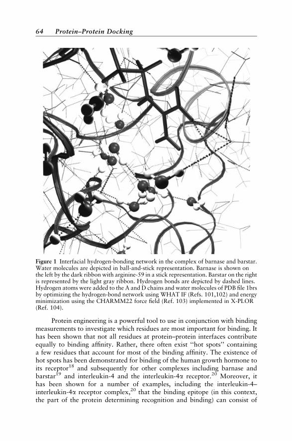
Protein engineering is a powerful tool to use in conjunction with bindingmeasurements to investigate which residues are most important for binding. Ithas been shown that not all residues at protein–protein interfaces contributeequally to binding affinity. Rather, there often exist ‘‘hot spots’’ containinga few residues that account for most of the binding affinity. The existence ofhot spots has been demonstrated for binding of the human growth hormone toits receptor18 and subsequently for other complexes including barnase andbarstar19 and interleukin-4 and the interleukin-4a receptor.20 Moreover, ithas been shown for a number of examples, including the interleukin-4–interleukin-4a receptor complex,20 that the binding epitope (in this context,the part of the protein determining recognition and binding) can consist of

Figure 1 Interfacial hydrogen-bonding network in the complex of barnase and barstar.Water molecules are depicted in ball-and-stick representation. Barnase is shown onthe left by the dark ribbon with arginine-59 in a stick representation. Barstar on the rightis represented by the light gray ribbon. Hydrogen bonds are depicted by dashed lines.Hydrogen atoms were added to the A and D chains and water molecules of PDB file 1brsby optimizing the hydrogen-bond network using WHAT IF (Refs. 101,102) and energyminimization using the CHARMM22 force field (Ref. 103) implemented in X-PLOR(Ref. 104).

64 Protein–Protein Docking

two distinct but overlapping epitopes: one containing residues of primaryimportance for the dissociation rate, the other containing residues of mostimportance for the association rate. The association rate will be most depen-dent on mutation of residues making contacts in the diffusional encountercomplex,21 whereas the dissociation rate will be dependent on the structureof the bound complex. This difference can be exploited for the design ofmutants in which the association rate, but not the dissociation rate, is altered.22

The binding affinity of two proteins is frequently the result of enthalpy–entropy compensation. Ideally, then, the estimation of the binding affinityduring protein–protein docking should include the computation of bothenthalpies and entropies of binding,23 thus enabling estimation of the tempera-ture dependence of the binding affinity. However, enthalpy–entropy compen-sation makes it difficult to account for these two terms explicitly24 whileproviding fast, accurate estimates of binding affinity during docking. Further,there is relatively little calorimetric data available on protein–protein bindingfor calibrating the empirical functions used to estimate enthalpies and entro-pies. However, some systematic studies have been carried out to perform coor-dinated calorimetric experiments and computations.25 Good agreementbetween experiment and the structural energetic calculations (in which ther-modynamic parameters are estimated based upon changes that occur in polarand apolar solvent-accessible surface area) have been obtained.26,27

Protein–protein binding energetics are influenced not only by the proteinsequence and structure, but also by the conditions under which binding takesplace. The pH is an important parameter, and pH dependence has been mea-sured for protein–protein binding affinity.19,28 Sensitivity to pH arises fromchanges in the ionization state of residues important for binding. For example,Schreiber and Fersht29 could attribute the pH dependence of barnase–barstarunbinding to a single barnase histidine residue. Ionic strength can also affiectbinding, particularly when electrostatic interactions are strong. There can bespecific ion-binding efects that can affiect the stability of the proteins and theirbinding thermodynamics, as exemplified by phosphate ion binding.25 Finally,the viscosity of the solvent can affect the binding kinetics; viscogens exertosmotic pressure and thus alter binding affinity.30

There are several energetic contributions to protein–protein binding affi-nity. The relative importance of hydrophobic and electrostatic interactionsvaries in diffierent complexes. So too does the contribution of individual watermolecules and specific hydrogen bonds. Protein–protein interfaces do notgenerally show charge complementarity, but, due to the long-range natureof electrostatic interactions and the heterogeneity of the protein–solventdielectric environment, they do show complementarity of their surface electro-static potentials.31 Therefore, it is not a straightforward task to derive simpleexpressions that are universally applicable to estimating binding affinity.However, correlations between experimental binding affinities and relativelysimple additive energy functions that depend on interfacial properties havebeen obtained.32,33

Introduction 65

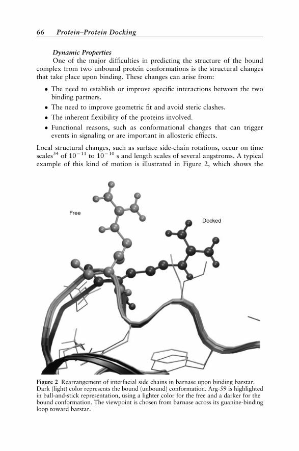
Dynamic PropertiesOne of the major difficulties in predicting the structure of the bound

complex from two unbound protein conformations is the structural changesthat take place upon binding. These changes can arise from:

* The need to establish or improve specific interactions between the twobinding partners.

* The need to improve geometric fit and avoid steric clashes.

* The inherent flexibility of the proteins involved.

* Functional reasons, such as conformational changes that can triggerevents in signaling or are important in allosteric effiects.

Local structural changes, such as surface side-chain rotations, occur on timescales34 of 1011 to 1010 s and length scales of several angstroms. A typicalexample of this kind of motion is illustrated in Figure 2, which shows the

FreeDocked

Figure 2 Rearrangement of interfacial side chains in barnase upon binding barstar.Dark (light) color represents the bound (unbound) conformation. Arg-59 is highlightedin ball-and-stick representation, using a lighter color for the free and a darker for thebound conformation. The viewpoint is chosen from barnase across its guanine-bindingloop toward barstar.

66 Protein–Protein Docking

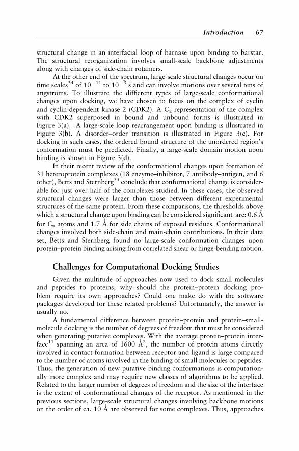
structural change in an interfacial loop of barnase upon binding to barstar.The structural reorganization involves small-scale backbone adjustmentsalong with changes of side-chain rotamers.

At the other end of the spectrum, large-scale structural changes occur ontime scales34 of 1011 to 103 s and can involve motions over several tens ofangstroms. To illustrate the diffierent types of large-scale conformationalchanges upon docking, we have chosen to focus on the complex of cyclinand cyclin-dependent kinase 2 (CDK2). A Ca representation of the complexwith CDK2 superposed in bound and unbound forms is illustrated inFigure 3(a). A large-scale loop rearrangement upon binding is illustrated inFigure 3(b). A disorder–order transition is illustrated in Figure 3(c). Fordocking in such cases, the ordered bound structure of the unordered region’sconformation must be predicted. Finally, a large-scale domain motion uponbinding is shown in Figure 3(d).

In their recent review of the conformational changes upon formation of31 heteroprotein complexes (18 enzyme–inhibitor, 7 antibody–antigen, and 6other), Betts and Sternberg35 conclude that conformational change is consider-able for just over half of the complexes studied. In these cases, the observedstructural changes were larger than those between different experimentalstructures of the same protein. From these comparisons, the thresholds abovewhich a structural change upon binding can be considered significant are: 0.6 A

for Ca atoms and 1.7 A for side chains of exposed residues. Conformationalchanges involved both side-chain and main-chain contributions. In their dataset, Betts and Sternberg found no large-scale conformation changes uponprotein–protein binding arising from correlated shear or hinge-bending motion.

Challenges for Computational Docking Studies

Given the multitude of approaches now used to dock small moleculesand peptides to proteins, why should the protein–protein docking pro-blem require its own approaches? Could one make do with the softwarepackages developed for these related problems? Unfortunately, the answer isusually no.

A fundamental difference between protein–protein and protein–small-molecule docking is the number of degrees of freedom that must be consideredwhen generating putative complexes. With the average protein–protein inter-face11 spanning an area of 1600 A2, the number of protein atoms directlyinvolved in contact formation between receptor and ligand is large comparedto the number of atoms involved in the binding of small molecules or peptides.Thus, the generation of new putative binding conformations is computation-ally more complex and may require new classes of algorithms to be applied.Related to the larger number of degrees of freedom and the size of the interfaceis the extent of conformational changes of the receptor. As mentioned in theprevious sections, large-scale structural changes involving backbone motionson the order of ca. 10 A are observed for some complexes. Thus, approaches

Introduction 67

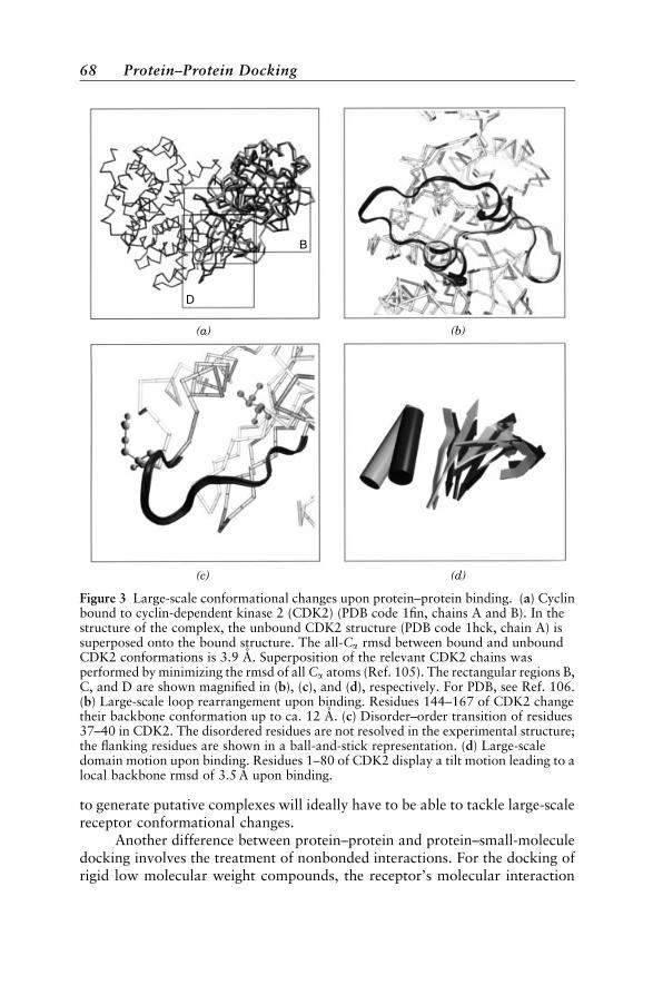
to generate putative complexes will ideally have to be able to tackle large-scalereceptor conformational changes.

Another difference between protein–protein and protein–small-moleculedocking involves the treatment of nonbonded interactions. For the docking ofrigid low molecular weight compounds, the receptor’s molecular interaction

(b)

(d)

(a)

(c)

D

B

Figure 3 Large-scale conformational changes upon protein–protein binding. (a) Cyclinbound to cyclin-dependent kinase 2 (CDK2) (PDB code 1fin, chains A and B). In thestructure of the complex, the unbound CDK2 structure (PDB code 1hck, chain A) issuperposed onto the bound structure. The all-Ca rmsd between bound and unboundCDK2 conformations is 3.9 A. Superposition of the relevant CDK2 chains wasperformed by minimizing the rmsd of all Ca atoms (Ref. 105). The rectangular regions B,C, and D are shown magnified in (b), (c), and (d), respectively. For PDB, see Ref. 106.(b) Large-scale loop rearrangement upon binding. Residues 144–167 of CDK2 changetheir backbone conformation up to ca. 12 A. (c) Disorder–order transition of residues37–40 in CDK2. The disordered residues are not resolved in the experimental structure;the flanking residues are shown in a ball-and-stick representation. (d) Large-scaledomain motion upon binding. Residues 1–80 of CDK2 display a tilt motion leading to alocal backbone rmsd of 3.5 A upon binding.

68 Protein–Protein Docking

fields, such as the electrostatic potential, can often be computed and storedprior to the docking simulation. On the other hand, the more extensive con-formational changes occurring during protein–protein binding require updat-ing of these computationally expensive quantities during docking. Thus,scoring functions for protein–protein docking either have to treat these inter-actions in a heuristic way or they must invoke more efficient techniques for theevaluation of the expensive nonbonded interactions.

In the following section, we describe computational approaches used inthe protein–protein docking field. We focus mostly on the aspect of generatingputative complex structures. Although some small molecule docking programshave been extended for application to protein–protein docking as well, mostapproaches representnewefforts targetedspecificallyatprotein–proteindocking.

COMPUTATIONAL APPROACHESTO THE DOCKING PROBLEM

In this section, we present an overview of the methods currently in usefor docking binary protein complexes. Although docking of ternary proteincomplexes has been reported,36 the majority of computational studies todate deal with the case of two interacting proteins.

Manual docking approaches have long been used for generating protein–protein complexes. These approaches require the researcher to dock the twoproteins interactively and determine the chemical and geometric fit by meansof computer graphics tools. Preliminary structures of complexes generatedmanually can be refined to remove bad contacts by energy minimization. Man-ual docking is often done by using experimental data on the effects of muta-tions as guides for generating plausible structures of complexes. Anderson andWeng37 described an advanced approach for manual protein–protein dockingutilizing immersive virtual reality environments such as haptic devices that cre-ate a sense of touch via controlled force feedback to the user’s hand. Althoughthey could demonstrate successful protein–protein docking in two cases usingvirtual reality, no large-scale applications have been reported so far.

Two general categories of approaches to automated protein–proteindocking can be distinguished. In the first, rigid-body docking, both proteinsare considered to be completely rigid, thereby reducing the docking problemto a search through six degrees of freedom for the optimal orientation. Rigid-body docking approaches are usually geared toward optimizing the geometricand/or chemical fit of the two proteins. Typical execution times on currentcomputer hardware are on the order of minutes for representative enzyme–inhibitor complexes. This computational efficiency enables the user to auto-matically screen databases of proteins for mutual interactions. On the otherhand, conformational rearrangements of the proteins and interfacial solvationare not treated in any of the rigid-body docking approaches.

Computational Approaches to the Docking Problem 69

In the second approach, flexible docking, protein conformational flex-ibility is treated explicitly. The extent to which protein flexibility is modeledvaries. Some approaches account for the relative motions of protein domains,others account for rotation of amino acid side chains, and others treat allatomic degrees of freedom. These approaches are based on minimizing energyor on optimizing shape-based criteria, or on performing atomic-detail simula-tions that allow a time interpretation of the binding process. Naturally, execu-tion speeds can be extensive, ranging from hours to days for a single dockingon current computing hardware. Typically, the value of fine-grained flexibledocking approaches is to understand an interesting binding event particularlywell. Screening databases with thousands of putative interaction partners isout of the reach of current flexible docking methods due to their computa-tional demands.

Docking = Sampling + Scoring

Throughout this chapter, we roughly separate docking approaches bytheir treatment of protein flexibility. Within the two broad categories (rigidbody and flexible docking), the docking problem can be separated into twosubproblems:

1. The sampling problem: Given two independent protein structures, generateputative structures of the complex.

2. The scoring problem: Given a set of putative complexes, rank them byestimating their free energy of binding.

A plethora of techniques has been employed to address the sampling problem,ranging from complete enumeration of the relative orientations of the rigidbinding partners to methods based on effective energy gradients to determinenew atomic positions.

For the scoring problem, the free energy of binding for a certain putativecomplex has to be estimated. These estimates should take into account boththe enthalpic and the entropic contributions to the free energy of binding.Although free energy perturbation38–41 techniques employing moleculardynamics simulations for sampling can be applied to protein–protein bind-ing,42 they are too demanding in terms of computational resources to be ofpractical value for docking problems at present. Instead, a common strategyis to use heuristic techniques to estimate the entropic component of the freeenergy of binding (e.g., desolvation energies are parameterized by atomic sol-vation parameters43), and simplified potential energy functions are used toestimate the enthalpic component. A simple scoring function might be givenby the number of intermolecular contacts shorter than a given threshold dis-tance or the number of van der Waals (vdW) clashes in the protein–proteininterface. A slightly more complex scoring function would account for the che-mical nature of the interacting atoms of the proteins as well as their spatial

70 Protein–Protein Docking

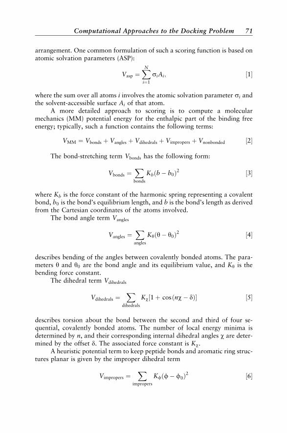
arrangement. One common formulation of such a scoring function is based onatomic solvation parameters (ASP):

Vasp ¼XNi¼1

siAi; ½1

where the sum over all atoms i involves the atomic solvation parameter si andthe solvent-accessible surface Ai of that atom.

A more detailed approach to scoring is to compute a molecularmechanics (MM) potential energy for the enthalpic part of the binding freeenergy; typically, such a function contains the following terms:

VMM ¼ Vbonds þ Vangles þ Vdihedrals þ Vimpropers þ Vnonbonded ½2

The bond-stretching term Vbonds has the following form:

Vbonds ¼Xbonds

Kbðb b0Þ2 ½3

where Kb is the force constant of the harmonic spring representing a covalentbond, b0 is the bond’s equilibrium length, and b is the bond’s length as derivedfrom the Cartesian coordinates of the atoms involved.

The bond angle term Vangles

Vangles ¼X

angles

Kyðy y0Þ2 ½4

describes bending of the angles between covalently bonded atoms. The para-meters y and y0 are the bond angle and its equilibrium value, and Ky is thebending force constant.

The dihedral term Vdihedrals

Vdihedrals ¼X

dihedrals

Kw½1 þ cosðnw dÞ ½5

describes torsion about the bond between the second and third of four se-quential, covalently bonded atoms. The number of local energy minima isdetermined by n, and their corresponding internal dihedral angles w are deter-mined by the offset d. The associated force constant is Kw.

A heuristic potential term to keep peptide bonds and aromatic ring struc-tures planar is given by the improper dihedral term

Vimpropers ¼X

impropers

Kfðf f0Þ2 ½6

Computational Approaches to the Docking Problem 71

Here, a pseudo-dihedral angle is defined similarly to a dihedral angle and isdenoted by f. The respective force constant is Kf.

The Coulombic and vdW interactions are represented by the nonbondedpotential term

Vnonbonded ¼X

nonbonded

eRminij

rij

12

2Rminij

rij

6" #

þ qiqj

Drij

!½7

Here, the interatomic distance between atoms i and j is rij. The depth of theLennard-Jones well describing the vdW interaction is given by e, and the loca-tion of its minimum is given by Rminij

. The electrostatic interaction is repre-sented by charges qi, qj, the interaction of which is modified by an effectivedielectric constant D.

Electrostatic desolvation effects upon binding can be scored by invokinga Poisson–Boltzmann (PB) formulation of electrostatic binding energies44 ofthe form

VPB ¼ 1

2

ðr/d3r ½8

where r is the total charge density and the electrostatic potential / is given bysolution of the PB equation

r er/ ¼ r f þ lX

i

ciqi exp qi/=kBTð Þ ½9

Here, r f denotes the fixed charge distribution of the proteins, and e theposition-dependent permittivity. The term r er/ represents the divergenceof the displacement field and, according to Gauss’s law, is equal to the chargedensity. The ionic charge density is given by liciqi exp ðqi/=kBTÞ, whereions of charge qi have a bulk concentration of ci, and l ¼ 1 in ion accessibleregions and l ¼ 0 elsewhere.

Although the sampling and the scoring problems are conceptually differ-ent in nature, their solutions are not independent. The complexity of theenergy landscape, which is dependent on factors such as the smoothing andresolution of the scoring function, will influence the extent and type of sam-pling required. Although efforts to solve the sampling and scoring problemsare intertwined, we will describe current approaches to solve the two problemsseparately. Summaries of the methods discussed and their respective technicalcomponents are given in Tables 1 and 2. Because the run times given in thesetables for the individual methods were obtained for computations on differentcomputer hardware and example protein–protein complexes, they should beconsidered only as rough relative estimates.

72 Protein–Protein Docking

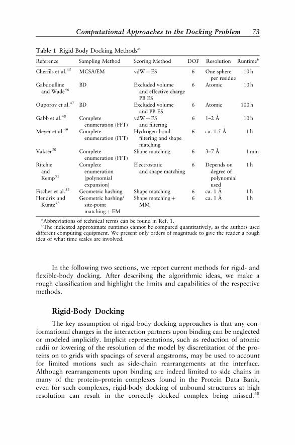
In the following two sections, we report current methods for rigid- andflexible-body docking. After describing the algorithmic ideas, we make arough classification and highlight the limits and capabilities of the respectivemethods.

Rigid-Body Docking

The key assumption of rigid-body docking approaches is that any con-formational changes in the interaction partners upon binding can be neglectedor modeled implicitly. Implicit representations, such as reduction of atomicradii or lowering of the resolution of the model by discretization of the pro-teins on to grids with spacings of several angstroms, may be used to accountfor limited motions such as side-chain rearrangements at the interface.Although rearrangements upon binding are indeed limited to side chains inmany of the protein–protein complexes found in the Protein Data Bank,even for such complexes, rigid-body docking of unbound structures at highresolution can result in the correctly docked complex being missed.48

Table 1 Rigid-Body Docking Methodsa

Reference Sampling Method Scoring Method DOF Resolution Runtimeb

Cherfils et al.45 MCSA/EM vdW þ ES 6 One sphere 10 hper residue

Gabdoulline BD Excluded volume 6 Atomic 10 hand Wade46 and effective charge

PB ESOuporov et al.47 BD Excluded volume 6 Atomic 100 h

and PB ESGabb et al.48 Complete vdW þ ES 6 1–2 A 10 h

enumeration (FFT) and filteringMeyer et al.49 Complete Hydrogen-bond 6 ca. 1.5 A 1 h

enumeration (FFT) filtering and shapematching

Vakser50 Complete Shape matching 6 3–7 A 1 minenumeration (FFT)

Ritchie Complete Electrostatic 6 Depends on 1 hand enumeration and shape matching degree ofKemp51 (polynomial polynomial

expansion) usedFischer et al.52 Geometric hashing Shape matching 6 ca. 1 A 1 hHendrix and Geometric hashing/ Shape matching þ 6 ca. 1 A 1 h

Kuntz53 site-point MMmatchingþ EM

aAbbreviations of technical terms can be found in Ref. 1.bThe indicated approximate runtimes cannot be compared quantitatively, as the authors used

different computing equipment. We present only orders of magnitude to give the reader a roughidea of what time scales are involved.

Computational Approaches to the Docking Problem 73

Low-resolution rigid-body docking can be applied to a wide range of protein–protein complexes. These must display low-resolution recognition, a propertyfound by Vakser et al.60 to be present in more than half of the complexes in aset of ca. 500 nonredundant protein–protein complex crystal structures.

Gradient-Based TechniquesA variety of techniques has been developed to explore the conforma-

tional space spanned by the six degrees of freedom considered in rigid-bodydocking. In early work, Cherfils et al.45 parameterized protein–protein orien-tations by the protein separation distance along the line connecting the centersof mass and five variables for the respective angular orientations. For each setof these five angular variables, the optimal separation distance was computedby a simple scheme resulting in the smallest mutual separation without stericclashes. Steric clashes were computed with a low-resolution model in whicheach residue is replaced by a single sphere. For each given set of angular para-meters, the closest separation distance was determined, and an approximateinteraction energy comprising simple repulsive vdW-like and surface burialterms was computed. The five-dimensional space of angular variables was

Table 2 Flexible Docking Methodsa

Sampling ScoringReference Methods Methods DOF Resolution Runtimeb

Sandak et al.54 Geometric Shape 6þ 3Ndiscretehinge

c 2 A 10 minhashing matching

Jackson et al.55 Mean-field vdW þ ES and 6þ Ndiscreterotamers

d ca. 1 A 10 minequation desolvation

energyAlthaus et al.56 Optimization MM and Ndiscrete

rotamersd, Atomic 1 h

(DEE, LP) MM þ Natomsf

and EM desolvationWeng et al.57 Complete Effective free Ndiscrete

torsionse, Atomic Not given

enumeration energy Natomsf

(ASP/PB) or MMand EM

Abagyan et al.58 MCSA/EM MMþ Arbitrary Atomic 10 hdesolvationor MM

Ullmann et al.59 MCSAþ Colulombic þ 6, then Atomic Not givenMD/EM MM þ PB/SA 3Natoms

f

aAbbreviations of technical terms can be found in Ref. 1.bThe indicated approximate runtimes cannot be compared quantitatively, as the authors used

different computing equipment. We present only orders of magnitude to give the reader a roughidea of what time scales are involved.

cThe total number of hinges assumed for the flexible protein.dThe total number of rotameric states for all residues considered.eThe total number of variable torsional angles.f The number of atoms.

74 Protein–Protein Docking

searched by performing Monte Carlo simulated annealing and energy minimi-zation in random subspaces. Sets of candidate complexes generated by repeatedapplication of this searching technique were further energy minimized using anatomic level molecular mechanics force field. With this method, complexesclose to the experimental structure could be generated when starting fromthe respective bound conformations. However, docking of the unboundprotein structures in two test cases resulted in significant loss of interproteinhydrogen bonds, thus indicating the shortcomings of the method in dealingwith minor induced fit. Recently, this approach was used by Janin61 to gener-ate transition state complexes for the barnase–barstar system in order to studythe kinetics of this protein–protein binding event.

An alternative to the energy minimization approach of Cherfils et al.,45 isstochastic or Brownian dynamics (BD)62 in which bimolecular association tra-jectories are simulated, thus allowing for a time interpretation of the bindingprocess. In the work of Gabdoulline and Wade,46;63 BD simulations are usedto determine the association rates of proteins, given a known structure of thecomplex of the two proteins. Instead of generating a single bound complex,clusters of diffusional encounter complexes21 are obtained by simulatingmany trajectories. Intermolecular excluded volume and electrostatic interac-tions are used to derive the forces. An effective charge model64 is used to com-pute approximate Poisson–Boltzmann electrostatic forces in an efficientmanner. Brownian dynamics can also be used to predict the structures of elec-trostatically favorable docked protein–protein complexes, as was recentlydemonstrated by Ouporov et al.47

Complete EnumerationInstead of finding the optimal six-dimensional coordinate set by gradient-

based methods, an alternative approach is to discretize all dimensions andlocate the approximate optimum complex by complete enumeration. Withthe number of points in each direction being N, a naive enumeration wouldhave a computational complexity of O(N6). This approach is illustrated byrecent work of Palma et al.,65 who use a binary representation of each proteinon a cubic grid. For a given grid, each grid point is assigned a value of 0 whenno atom is close, and 1 otherwise. For a given relative orientation of two pro-teins, their geometric fit can then be determined by efficient binary computa-tions of the representative grids. The best preliminary orientations are thenscored using electrostatic and surface matching, and pairwise residue potentialterms. These scores are combined by means of a neural network to derive asingle score for a given orientation.

An alternative for identifying the optimal rigid-body orientation is pro-vided by the convolution-based strategy pioneered by Katchalski-Katzir et al.66

If the scoring function is cast into the shape of a mathematical correlationfunction, the complexity can be reduced to O(N3 log(N3)). Figure 4 illustratesthe main idea of the algorithm. First, the three angular variables are separated

Computational Approaches to the Docking Problem 75

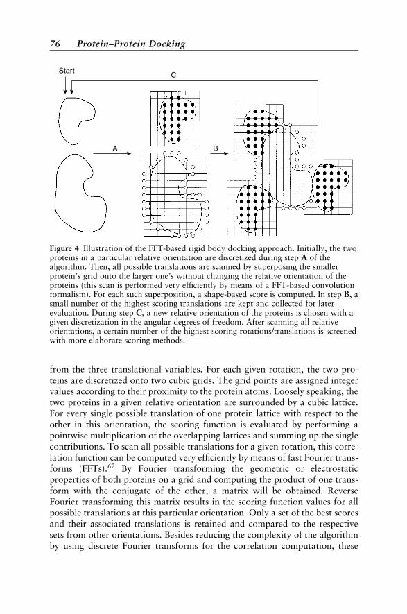
from the three translational variables. For each given rotation, the two pro-teins are discretized onto two cubic grids. The grid points are assigned integervalues according to their proximity to the protein atoms. Loosely speaking, thetwo proteins in a given relative orientation are surrounded by a cubic lattice.For every single possible translation of one protein lattice with respect to theother in this orientation, the scoring function is evaluated by performing apointwise multiplication of the overlapping lattices and summing up the singlecontributions. To scan all possible translations for a given rotation, this corre-lation function can be computed very efficiently by means of fast Fourier trans-forms (FFTs).67 By Fourier transforming the geometric or electrostaticproperties of both proteins on a grid and computing the product of one trans-form with the conjugate of the other, a matrix will be obtained. ReverseFourier transforming this matrix results in the scoring function values for allpossible translations at this particular orientation. Only a set of the best scoresand their associated translations is retained and compared to the respectivesets from other orientations. Besides reducing the complexity of the algorithmby using discrete Fourier transforms for the correlation computation, these

A

C

B

Start

Figure 4 Illustration of the FFT-based rigid body docking approach. Initially, the twoproteins in a particular relative orientation are discretized during step A of thealgorithm. Then, all possible translations are scanned by superposing the smallerprotein’s grid onto the larger one’s without changing the relative orientation of theproteins (this scan is performed very efficiently by means of a FFT-based convolutionformalism). For each such superposition, a shape-based score is computed. In step B, asmall number of the highest scoring translations are kept and collected for laterevaluation. During step C, a new relative orientation of the proteins is chosen with agiven discretization in the angular degrees of freedom. After scanning all relativeorientations, a certain number of the highest scoring rotations/translations is screenedwith more elaborate scoring methods.

76 Protein–Protein Docking

methods offer the potential for computational efficiency. Whereas theFTDOCK package of Gabb et al.48 has a parallel implementation of theFFTs on a shared-memory architecture, the DOT program68;69 utilizes afarmer/worker approach to distribute sets of orientations between workernodes in a distributed memory environment. In this approach, one controlprocessor (the farmer) distributes tasks to identical worker processes, whichcompute and return the result.

Different types of scoring function can be applied in combination withconvolution-based docking. In FTDOCK, a geometric matching score isused to generate complexes, whereas electrostatics is applied only as a poster-ior binary filter. In DOT, electrostatic and geometric scores are used in con-junction during generation of complexes. Electrostatic computations areperformed in FTDOCK with a Coulombic formalism, a distance-dependentdielectric constant, and point charges interpolated on a grid. In contrast,DOT can utilize the output of software suites such as UHBD70 or DelPhi71

that compute electrostatic potentials as solutions to the Poisson-Boltzmannequation.44 Both FTDOCK and DOT use an atomic representation of theproteins involved to derive the discretized protein grid. All fine-grainedconvolution-based docking approaches are demanding with respect to mem-ory usage: to perform the FFTs efficiently, grids of N3 complex numbersmust be kept in memory. For large proteins, this necessitates minimum gridspacings larger than 1 A, and therefore the protein might not be representedat the resolution desired.

An efficient implementation, useful for low-resolution docking, has beenprovided by Vakser and Aflalo in their GRAMM package.72 This programprovides an implementation of the approach of Katchalski-Katzir et al.,66

employing a coarse grid with a grid spacing up to 7 A to represent the inter-acting proteins.50 Although a grid spacing of 7 A might not be useful fordetecting the impact of single-residue mutations on protein–protein associa-tion, this approach can help to detect the proper binding hemispheres for largesets of proteins.60 A modified version of the algorithm considers only hydro-phobic contacts for the geometric surface matching;72 this modification wasshown to improve the scores of the correct positive results compared to thefalse positives. Low-resolution docking, as implemented in GRAMM, appearsstrongly influenced by the choice of the parameters describing the proteinshape, including the grid spacing;73 care must be taken to find the optimalparameter set for a given protein–protein docking problem.

In all of the correlation-based docking approaches described above, acomplete enumeration of the rotational angle space is performed. Meyeret al.49 modified the basic technique by filtering to select those relativerotations that lead to formation of at least two simultaneous intermolecularhydrogen bonds. This filtering is achieved by storing the directionality of thehydrogen-bond donor and acceptor sites in a translation-independent way.After performing the translational scans in the conventional manner, the

Computational Approaches to the Docking Problem 77

rotational parameters of the complexes, filtered to satisfy the hydrogen-bond-ing criteria, are further refined using a derivative-free minimization techniqueto optimize the geometric fit of the two proteins.

While retaining the formulation of the geometric and chemical fit as amathematical correlation, Ritchie and Kemp51 use a series expansion todescribe the shapes of the proteins. This mathematical description uses gener-alized Laguerre polynomials and spherical harmonics.67 Ritchie and Kempformulate the scoring function in one distance and five angular variables.With their mathematical framework, translations and rotations of the proteinscan be reduced to a recomputation of these expansion coefficients, which canbe carried out efficiently. After a coarse-grained global scan of all the variablesand evaluation of the peaks in the geometric part of the scoring function, afine-grained scan of the interesting parts of the configurational space is per-formed using the full geometric and electrostatic contributions. In contrastto the FFT-based docking schemes described above, the memory requirementsof the Ritchie–Kemp algorithm are relatively modest and do not depend on thesize of the proteins. As this technique is based on scanning the entire config-urational space, it offers the potential for parallelization as well. Moreover, itbecomes very efficient when the binding site on one of the proteins is known.In the spherical polar approach, this can be specified by a simple constraint inone or two angular degrees of freedom prior to evaluating correlations.

Geometric Hashing TechniquesAs an alternative to completely enumerating all relative orientations,

Fischer et al.52 reported the development of a computer-vision-based techni-que called geometric hashing. This scheme is conceptually similar to that uti-lized in the DOCK program53;74 which tries to find matches in the internaldistances between spheres74 or shape-based site-points,53 which represent thesurface features of the proteins.

By construction, the geometric hashing method generates only com-plexes with at least partial geometric fit, which is achieved by storing criticalpoint information (position or surface normals) with respect to locally definedcoordinate systems (derived from sets of critical points themselves). Utilizingefficient data structures, matches of these local coordinate systems are rankedby the number of ligand and receptor critical points that are in close proxi-mity. For the highest scoring pairs of local coordinate systems, the geometrictransforms that bring them into overlap are computed in an iterative fashion.After filtering the resulting set of possible ligand transformations by a scoringscheme (e.g., based on buried surface area), a set of candidate complexes isgenerated. The complexity of the algorithm is O(N3), with N being thenumber of receptor critical points. In the implementation of Fischer et al.,52

the number of receptor critical points is about 0.3–1 times the number ofsurface atoms on the receptor (and ranges from ca. 60 to 600 for the set ofrepresentative proteins that they studied).

78 Protein–Protein Docking

Flexible Docking

In this section, we describe some of the current methods for treatingprotein flexibility explicitly during docking. We order the methods accordingto the level of flexibility covered, starting with large-scale motion betweenrigid domains and ending with full atomic flexibility.

Geometric Hashing TechniquesOne particular type of large-scale motion, hinge bending, is treated in a

modified75 version of the geometric hashing algorithm of Nussinov and co-workers.52;54 In the modified approach (illustrated in Figure 5), the usermust specify the position of the hinge(s) (several hinges are possible) in the‘‘ligand’’ protein prior to starting the docking procedure. Triangles spannedby triples of critical points of both proteins are precomputed; each such trian-gle is characterized by its side lengths. The location and orientation of such aligand triangle with respect to a hinge is stored as a translation vector and arotation transform during the preprocessing phase of the algorithm. In therecognition (i.e., sampling) phase of the algorithm, the triangles spanned bycritical points on the surface of the receptor protein are matched to those com-puted for the flexible ligand protein. When a match is found, application of thestored transformation to the current trial ligand protein coordinate frameresults in the putative hinge position and orientation. This hinge positionand orientation is stored and receives a ‘‘vote.’’ When different parts of theligand protein vote for the same hinge location, the entire protein can bereconstructed in a bent conformation. After such a reconstruction, candidatesare filtered with respect to steric clashes and scored by the percentage of theligand protein’s atoms in contact with the receptor protein. The algorithmnaturally extends to proteins with several hinges. Sandak et al.75 docked theM13 peptide to calmodulin. Although the algorithm can recover the dockedcomplex when starting from the single-bound conformations, the results forthe unbound protein conformation are significantly worse. One reason couldbe that the hinge motion implemented in the algorithm does not describe wellthe actual large-scale conformational changes of calmodulin.

Conformational Search TechniquesAs part of the suite of codes for flexible docking developed by Sternberg

et al.,76 the MULTIDOCK code55 optimizes the conformations of the interfa-cial side chains after obtaining the predicted docked orientation from a rigid-body docking procedure. The approach entails iterations until convergence ofthe interaction energy is attained. Each iteration comprises two steps: determi-nation of the best rotamers for interfacial side chains, and then small-scalerigid-body energy minimization. The energy terms used include mean-fieldterms for the bonded, electrostatic, van der Waals, and solvation contribu-tions. Whereas bonded interactions are only modeled approximately, by

Computational Approaches to the Docking Problem 79

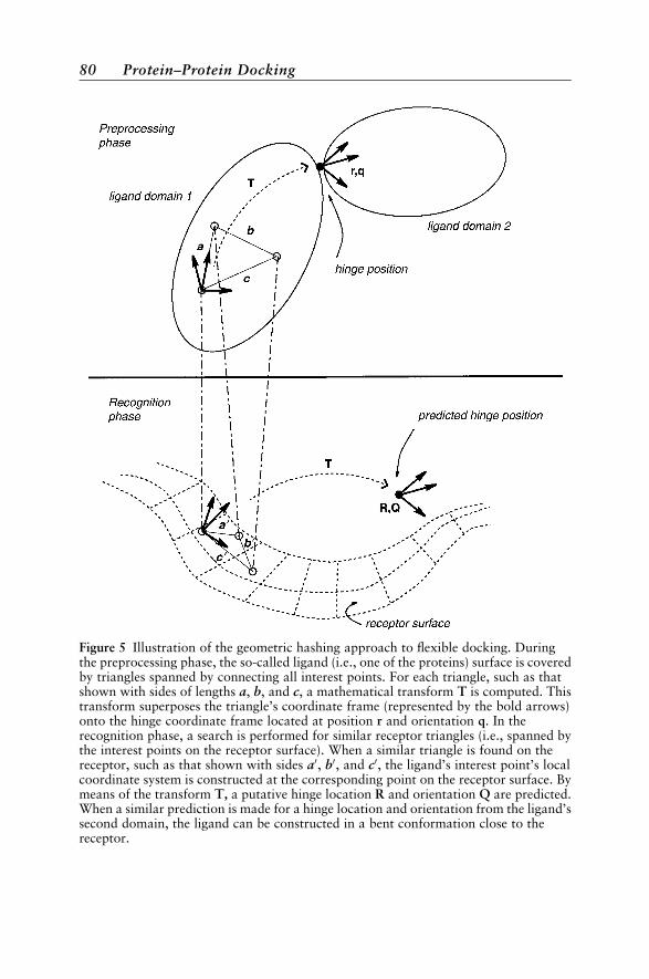
Figure 5 Illustration of the geometric hashing approach to flexible docking. Duringthe preprocessing phase, the so-called ligand (i.e., one of the proteins) surface is coveredby triangles spanned by connecting all interest points. For each triangle, such as thatshown with sides of lengths a, b, and c, a mathematical transform T is computed. Thistransform superposes the triangle’s coordinate frame (represented by the bold arrows)onto the hinge coordinate frame located at position r and orientation q. In therecognition phase, a search is performed for similar receptor triangles (i.e., spanned bythe interest points on the receptor surface). When a similar triangle is found on thereceptor, such as that shown with sides a0, b0, and c0, the ligand’s interest point’s localcoordinate system is constructed at the corresponding point on the receptor surface. Bymeans of the transform T, a putative hinge location R and orientation Q are predicted.When a similar prediction is made for a hinge location and orientation from the ligand’ssecond domain, the ligand can be constructed in a bent conformation close to thereceptor.

80 Protein–Protein Docking

assigning each rotamer an energy derived from observed side-chain rotamericpreferences in a rotamer library, the solvation term takes into account detailedinteractions with water molecules which are treated as soft sphere Langevindipoles on a grid that make vdW, electrostatic, and hydrophobic interactionswith the protein. The interaction with bulk solvent beyond the Langevindipoles grid around the protein is modeled by the Kirkwood equation (whichgives an expression for the electrostatic interaction energy of a solute’s mono-pole and dipole moments with a surrounding solvent dielectric continuum).The approach55 shows good improvement of the ranking of the complexesproposed by rigid-body docking approaches, but encounters difficultieswhen the complexes studied exhibit extensive side-chain rearrangements orbackbone motion. In addition, charged residues in nonrotameric states cannotbe modeled by the algorithm.

Althaus et al.56 use combinatorial optimization techniques to optimizethe discrete rotamers of interfacial side chains after generating candidate com-plexes with a Fourier-correlation based rigid-body docking approach. Duringside-chain optimization, the AMBER77 molecular mechanics energy functionis minimized. In the final scoring of the set of putative optimal complexes, amore elaborate energy function is used. This energy function includes contin-uum electrostatics, surface burial, protein conformational entropy, and vdWterms.

Two further energy functions based on Poisson-Boltzmann electrostaticsand atomic solvation parameter (ASP)-based parameterizations of the solva-tion free energy changes43 were evaluated by Weng et al.57 in the context ofside-chain optimization after rigid-body docking.

Gradient-Based TechniquesWhereas the side-chain optimization techniques described above confine

the side-chain conformations to discrete tabulated rotameric states, theapproach of Abagyan et al.58;78 considers the side-chain torsions as degreesof freedom in an optimization procedure. In their procedure, named ‘‘internalcoordinate mechanics,’’ a two-tier energy function is minimized with respectto arbitrary internal coordinates of the interacting proteins. The minimizationconsists of biased distortions of the conformations, followed by local energyminimization with respect to a molecular mechanics potential energy function.The new conformation is scored by an elaborate energy function including sur-face area dependent terms and a non-Coulombic electrostatic term accountingfor dielectric heterogeneity. The resulting score is used to accept the new con-formation on the basis of a Metropolis criterion (i.e., the probability of accep-tance is given by min[1,exp(E)], where E is the change in energy on goingfrom the current to the new conformation). The approach conceptually allowsfor limited backbone flexibility as well. The approach has been used success-fully for prediction of the lysozyme–HyHel5 antibody complex starting withlysozyme in the unbound conformation.78

Computational Approaches to the Docking Problem 81

Ullmann et al.59 developed a simulation-based approach that they usedto dock plastocyanin and cytochrome f. The method consisted of three stages.First, the proteins were held rigid in their unbound conformations and theirCoulombic interaction energy was minimized by running thousands of MonteCarlo trajectories in which the temperature was gradually cooled from 300 to0 K. Second, complexes with low Coulombic energy were refined by moleculardynamics simulation using the CHARMM force field79 with a spherical shellof explicit water molecules around plastocyanin and all atoms within theshell treated as mobile. The system was simulated at 300 K for 200 ps andthen gradually annealed to lower temperatures and energy minimized. Finallow-energy conformations were rescored with an energy function containingPoisson-Boltzmann electrostatic and solvent accessible surface area dependentterms. The configurations with the most favorable Coulombic interactionsdid not have the most favorable total energies, thus indicating the impor-tance of considering hydration and conformational flexibility. Severaldocked complexes were obtained by this procedure and could be used to in-terpret data on electron transfer between the proteins. Notably, the configura-tion with the most efficient electron transfer pathway did not have the lowestenergy.

EXAMPLE

In this section, we illustrate some of the methods described above (alongwith their limitations) when trying to dock two proteins from their respectiveunbound structures. This description does not aim at providing the optimalworkflow of such a project; we believe that right now, there is no one optimalmethodology for all classes of proteins. Instead, the type of docking experi-ment, the availability of experimental data, and the expected occurrence oflarge-scale motion for a particular protein will determine which selection ofthe approaches described above is likely to be feasible. In our example, wedescribe attempts at docking barnase, an experimentally well-characterizedextracellular ribonuclease, to its intracellular inhibitor, barstar.8082 The lim-ited degree of induced fit and wealth of experimental data, both kinetic andmutational,24;29;83 might suggest that this particular docking problem wouldbe easy to solve with a rigid-body docking approach. However, we showthat even such limited flexibility has an important impact on the results ofrigid-body docking. In our example, we aim to give the reader an idea ofhow the applicability of a certain method could be assessed. All in all, the sce-nario we have in mind is that of a researcher with plenty of time to dock asingle protein–protein complex. In this example, we do not address theproblem of detecting binding modes in large databases of proteins in anautomated fashion.

82 Protein–Protein Docking

Estimating the Extent of ConformationalChange upon Binding

Before applying a certain published method, it is worthwhile to estimatethe extent to which large-scale motion will occur for the proteins involved.One approach is to decompose correlated motions of atoms into so-calledmodes. This terminology stems from normal mode analysis84 of mechanicalsystems, which is based on evaluation of potential energy derivatives formechanical systems. Approximate techniques such as essential dynamics85

determine these modes from the positional fluctuations of selected atomsaround their mean in an ensemble of conformations by solving an eigenvalueproblem. Here, the eigenvectors of the position fluctuation matrix representindependent correlated motions of sets of atoms. As this technique does notrequire evaluations of potential energy derivatives or extensive energy minimi-zation, it is computationally much more applicable to an approximate predic-tion of the large-scale motions of a protein than normal mode analysis.Whereas the conformational ensembles in the original essential dynamicstechnique are generated by MD, the Concoord method developed by de Grootet al.86 perturbs a given protein structure on the basis of experimentallyobserved positional fluctuations. Thus, a conformational ensemble for use inan essential dynamics study can be generated at negligible computational cost.In Figure 6, the first collective mode of barnase is predicted by analyzing such aConcoord ensemble of conformations. Alternative techniques, such as thedetection of motion in a Gaussian network model87 or of independent domainmotions,88 differ in how they represent the protein and its potential energy,but represent efficient tools for predicting the large-scale motions of the asso-ciating proteins.

In Figure 6, the first essential mode of barnase’s is displayed. One parti-cularly flexible region is located around barnase’s arginine-59 which, frommutational studies,19;89 is known to contribute a large part of the free energyof binding. As this particular region is part of the binding interface, it is notclear whether reasonable predictions for the complex can be obtained by arigid-body docking approach starting from the unbound structures. Methodsto assess qualitatively the extent of large-scale flexibility can help in choosingan appropriate docking approach. In our barnase–barstar demonstration case,the superposition of bound and unbound structures reveals minor overallbackbone changes upon binding; the Ca rmsd is 0.5 A, although local rmsdsof up to 2 A are observed in the barnase–R59 region.

Rigid-Body Docking

When performing rigid-body docking with FTDOCK using the unboundprotein structures, without filtering by means of biochemical data, severalclusters are proposed by the program as illustrated in Figure 7. The major

Example 83

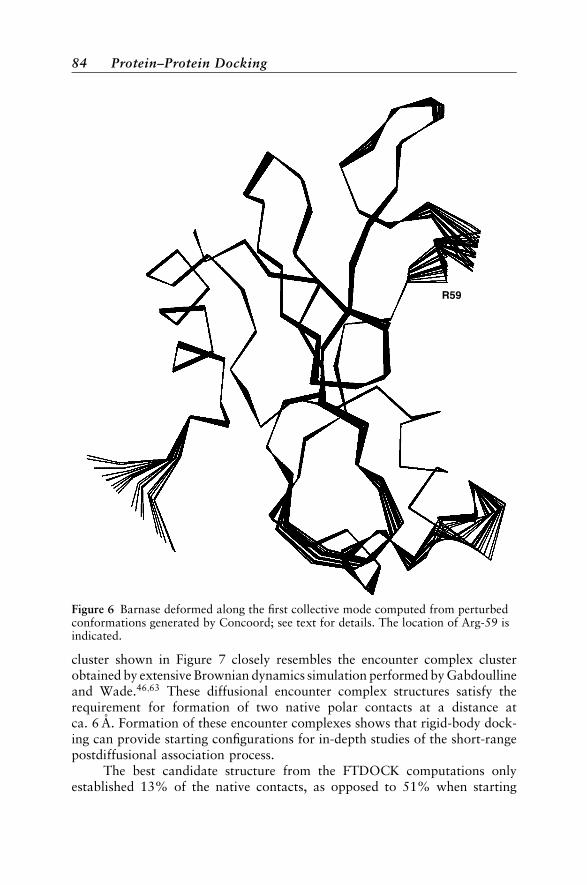
cluster shown in Figure 7 closely resembles the encounter complex clusterobtained by extensive Brownian dynamics simulation performed by Gabdoullineand Wade.46;63 These diffusional encounter complex structures satisfy therequirement for formation of two native polar contacts at a distance atca. 6 A. Formation of these encounter complexes shows that rigid-body dock-ing can provide starting configurations for in-depth studies of the short-rangepostdiffusional association process.

The best candidate structure from the FTDOCK computations onlyestablished 13% of the native contacts, as opposed to 51% when starting

R59

Figure 6 Barnase deformed along the first collective mode computed from perturbedconformations generated by Concoord; see text for details. The location of Arg-59 isindicated.

84 Protein–Protein Docking

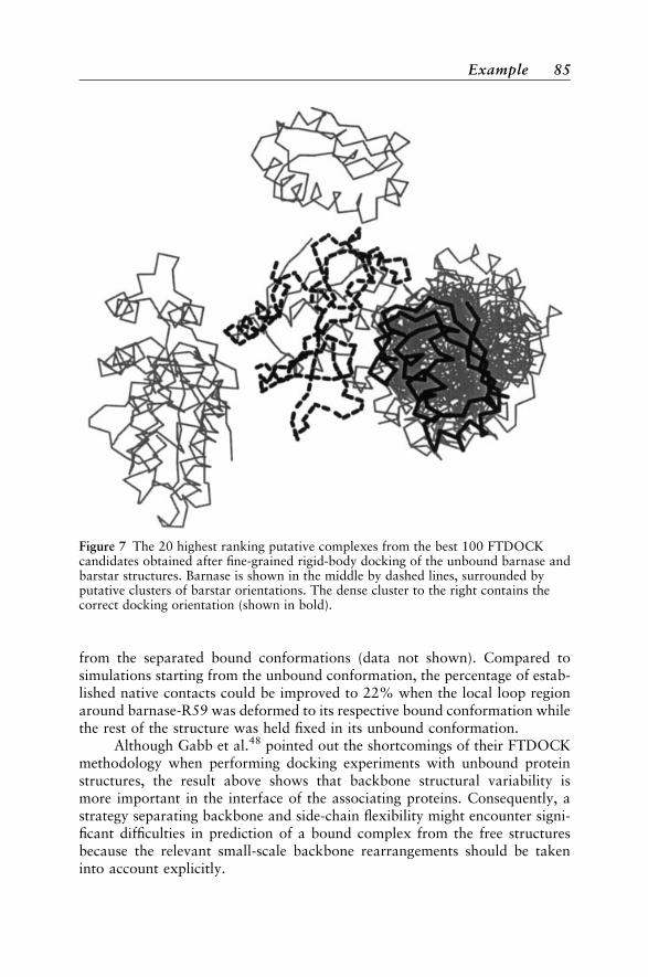
from the separated bound conformations (data not shown). Compared tosimulations starting from the unbound conformation, the percentage of estab-lished native contacts could be improved to 22% when the local loop regionaround barnase-R59 was deformed to its respective bound conformation whilethe rest of the structure was held fixed in its unbound conformation.

Although Gabb et al.48 pointed out the shortcomings of their FTDOCKmethodology when performing docking experiments with unbound proteinstructures, the result above shows that backbone structural variability ismore important in the interface of the associating proteins. Consequently, astrategy separating backbone and side-chain flexibility might encounter signi-ficant difficulties in prediction of a bound complex from the free structuresbecause the relevant small-scale backbone rearrangements should be takeninto account explicitly.

Figure 7 The 20 highest ranking putative complexes from the best 100 FTDOCKcandidates obtained after fine-grained rigid-body docking of the unbound barnase andbarstar structures. Barnase is shown in the middle by dashed lines, surrounded byputative clusters of barstar orientations. The dense cluster to the right contains thecorrect docking orientation (shown in bold).

Example 85

Flexible Docking with Side-Chain Flexibility

To test the impact of localized backbone and side-chain conformationalchanges when using an interface refinement strategy, we performed constrainedMD simulations in dihedral angle space90 (so-called torsion dynamics) ofbarnase–barstar association from an artificial starting arrangement similar tothose resulting from a rigid-body docking approach. In this starting conforma-tion, the two proteins were pulled apart along a line connecting their centers ofmass, leading to an rmsd of the interfacial barstar Ca atoms of 5 A. Using dif-ferent backbone conformations, only the side chains were allowed to move inthis all-atom, molecular dynamics simulation.

Whereas most side-chain optimization techniques described above relyon choosing one of a set of rotamers for a given side chain, the MD-basedsimulations can sample the full range of side-chain torsional angles. Treatingthese degrees of freedom as continuous is particularly relevant for so-calledhot spot residues88 such as barnase-R59, which contribute a large part tothe free energy of binding and do not occupy a standard rotameric state inthe bound complex. The favorable energy arising from the nonbonded inter-actions outweighs the unfavorable torsional energy of the nonstandardrotameric state.

Impact of Side-Chain Conformational ChangesBarnase-R59 has been shown to be involved in an intricate network of

water-mediated hydrogen-bonding interactions involving barstar and at leastfive ordered water molecules buried in the interface. Water molecules arerarely included explicitly in protein–protein docking studies; most approachesutilize implicit solvent approaches. In our torsion dynamics approach, themechanical properties of the solvent were taken into account by stochasticforces acting on surface protein atoms, and the solvent dielectric propertieswere represented by a distance-dependent dielectric constant. Thus, we canexpect that the use of this approximate model for the solvent will limit theaccuracy of predictions of the conformations and interactions of side-chainsinvolved in salt bridges or hydrogen bonds in the solvated interfacial region.As has been pointed out by Bogan and Thorn89 and Xu et al.,33 these residuesare often the ones that contribute most to the free energy of binding.

In our simulations, we performed association studies to elucidate theirrole by selecting pairs of those hot spot residues that established a barnase–barstar contact in the bound complex. In these simulations, we studied whateffect the side-chain conformation had on contact formation for certain hotspot residue pairs. A typical result is shown in Figure 8. Starting from the cor-rect rotameric state for certain hot spot residue pairs with the rest of the pro-teins in their unbound conformations leads to improved contact formation inthe initial docking phase. This effect is not observed when performing equiva-lent simulations with non-hot-spot interfacial residue pairs.

86 Protein–Protein Docking

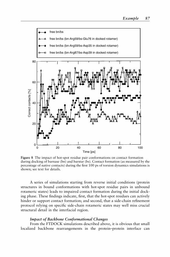
A series of simulations starting from reverse initial conditions (proteinstructures in bound conformations with hot-spot residue pairs in unboundrotameric states) leads to impaired contact formation during the initial dock-ing phase. These findings indicate, first, that the hot-spot residues can activelyhinder or support contact formation; and second, that a side-chain refinementprotocol relying on specific side-chain rotameric states may well miss crucialstructural detail in the interfacial region.

Impact of Backbone Conformational ChangesFrom the FTDOCK simulations described above, it is obvious that small

localized backbone rearrangements in the protein–protein interface can

free bn/bs

free bn/bs (bn-Arg59/bs-Glu76 in docked rotamer)

free bn/bs (bn-Arg59/bs-Asp35 in docked rotamer)

free bn/bs (bn-Arg87/bs-Asp39 in docked rotamer)

80

60

40

20

00 20 40 60 80 100

Time [ps]

Cor

rect

con

tact

s [%

]

Figure 8 The impact of hot-spot residue pair conformations on contact formationduring docking of barnase (bn) and barstar (bs). Contact formation (as measured by thepercentage of native contacts) during the first 100 ps of torsion dynamics simulations isshown; see text for details.

Example 87

influence the association process. To clarify the extent of this backbone effect,we performed side-chain torsion dynamics simulations using a barnase struc-ture with a deformed loop region surrounding barnase-R59. Starting from theunbound conformation, this loop region was deformed onto the Ca trace ofthe respective bound structure. This amounts to a local rmsd of 2 A, comparedto the 0.5-A overall backbone rmsd for the entire structure. Compared to priorsimulations with the unbound conformations, an improvement of up to 20%established contacts could be observed for the best in a series of simulations.The difference in docking progress between the bound and unbound startingconformation was almost compensated by introducing the proper backboneconformation in this binding-site loop.

Flexible Docking with Full Flexibility

Although side-chain torsion dynamics simulations can help in under-standing the influence of single residues and static backbone conformationson the binding process, they still neglect the effects arising from backbone flex-ibility. Standard molecular dynamics simulation techniques can be used as asampling tool to create putative complexes. However, unless simulations areperformed with suitable starting configurations close to the docked configura-tion, a major part of the simulation time will be spent exploring uninterestingregions of conformational space. At the other end of the spectrum, globalenergy minimization methods can be used to generate complexes while aban-doning the physical interpretation of the binding process.

Following an intermediate path, we developed a hybrid simulation me-thod to study the peculiarities of the barnase–barstar binding process. Thishybrid method was used to study the short-range association process. Simula-tions start with orientations resembling encounter complexes, obtained byrigid-body docking governed by long-range electrostatic interactions. Thishybrid simulation method is inspired by the genetic algorithm class of algo-rithms used for global optimization,91,92 in which entire ensembles of candi-dates are evaluated with respect to an optimality criterion and only promisingindividuals are propagated to the next generation. In our ‘‘ensemble enrich-ing’’ simulations, multiple copies of barnase interact with the mean field aris-ing from multiple copies of barstar and vice versa. No interaction is simulatedbetween copies of the same protein. In typical simulations, short (10 ps) simu-lations of 10 barnase and 10 barstar copies are performed with full atomicmobility. After each such simulation, all 100 possible complexes are scoredwith a heuristic energy function comprising nonbonded interaction energy,pairwise distance potentials, as well as implicit desolvation energy terms.These scores are used to derive an average fitness score for each proteincopy in the ensemble. Following this scoring stage, the five lowest scoring con-formations in each ensemble are discarded, and the remaining five are dupli-cated. This effectively leads to an enrichment of the promising candidate

88 Protein–Protein Docking

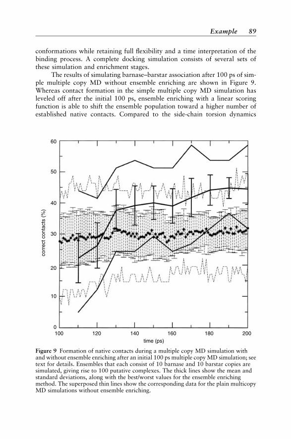
conformations while retaining full flexibility and a time interpretation of thebinding process. A complete docking simulation consists of several sets ofthese simulation and enrichment stages.

The results of simulating barnase–barstar association after 100 ps of sim-ple multiple copy MD without ensemble enriching are shown in Figure 9.Whereas contact formation in the simple multiple copy MD simulation hasleveled off after the initial 100 ps, ensemble enriching with a linear scoringfunction is able to shift the ensemble population toward a higher number ofestablished native contacts. Compared to the side-chain torsion dynamics

0100 120 140 160 180 200

10

20

30

40

50

60

time (ps)

corr

ect c

onta

cts

(%)

Figure 9 Formation of native contacts during a multiple copy MD simulation withand without ensemble enriching after an initial 100 ps multiple copy MD simulation; seetext for details. Ensembles that each consist of 10 barnase and 10 barstar copies aresimulated, giving rise to 100 putative complexes. The thick lines show the mean andstandard deviations, along with the best/worst values for the ensemble enrichingmethod. The superposed thin lines show the corresponding data for the plain multicopyMD simulations without ensemble enriching.

Example 89

simulation starting from the unbound conformations of both proteins, anadditional 20% of native contacts are gained when treating the simulated pro-teins as completely flexible. Some barnase copies with large numbers of estab-lished contacts exhibit a motion of the barnase–R59 loop region toward itsbound conformation.

Although the ensemble enriching multiple copy MD approach is cur-rently too demanding in terms of computational resources to be applied to alarge set of protein–protein complexes, it shows that simulations with fullyflexible proteins can be useful computational aids when no a priori limitationson flexibility should be made.

FUTURE DIRECTIONS

Computational protein–protein docking can be expected to be a veryactive field in the near future for several reasons. First, genomics and proteo-mics studies will provide large amounts of data on protein–protein binding.This binding data will often be of a qualitative kind (protein 1 interactswith protein 2), and computational studies will be necessary for detailed inter-pretation. Second, large-scale structural genomics studies will mean that 3Dstructures become available for many more protein targets of therapeuticinterest. However, it is anticipated that the structure of a target protein willoften be modeled by homology rather than be determined experimentally,and therefore may contain significant structural uncertainties and errors.These errors will be most apparent in loop regions, which can occur at theprotein-binding interface (e.g., as in antibody–antigen complexes). Thus, thesehomology models are a challenge for use in docking studies, and their inac-curacies mean that either low-resolution rigid-body docking strategies or stra-tegies that treat backbone and side-chain flexibility explicitly will be needed.Third, computational advances can be expected in both the sampling and thescoring aspects of docking methods.93

A range of computational docking methods will be required in this con-text and hierarchical approaches may be adopted so that computations are sui-ted to the type of data available and the questions to be answered. Forexample, screening of large protein data sets for protein–protein bindingrequires computationally efficient approaches such as sequence-based methodsand low-resolution rigid-body docking. These will be supported by techniquesto perform knowledge-based 3D structural searches of protein–protein bind-ing sites.94 When more experimental evidence about a particular complex isavailable (such as binding free energy differences from mutagenesis studies),the researcher can use these as conditions to filter proposed complexes froma low-resolution rigid-body docking approach. Then, a detailed atomisticmodel can be constructed and molecular flexibility treated.

90 Protein–Protein Docking

Computational developments in scoring functions can be expected tofocus particularly on solvation. There is presently considerable research effortdevoted to the development of new implicit solvation models (see, e.g., Ref. 95)and many of these models should be applicable to docking. Techniqueswill also be developed to include treatment of explicit water molecules inthe docking procedures. Currently, this can only be done during refinementof docked structures. In the small-molecule docking field, ways are beingdeveloped to consider interfacial water molecules explicitly during dock-ing.96,97 Related approaches can be expected to be developed for protein–protein docking.

As more computational docking methods are developed, stringent com-parisons of docking strategies, as in the Critical Assessment of Structure Pre-diction (CASP) project (http://predictioncenter.llnl.gov/),98,99 will be needed toevaluate which method is better suited for which problem class. AlthoughCASP does not include a docking section any longer, other forums such asthe Critical Assessment of Techniques for Free Energy Evaluation (CATFEE)project (http://uqbar.ncifcrf.gov/catfee/) may provide objective blind predic-tion tests for certain aspects of docking strategies. A complementary approachto compare and benchmark docking techniques is to establish a benchmark setof protein–protein docking problems against which new methods can be rou-tinely tested. This benchmark set should contain structurally diverse and ener-getically well-characterized protein–protein complexes. To test scoringfunctions, the experimentally determined protein–protein complexes shouldbe distinguished from decoy complexes. Sets of decoy complexes to test scor-ing functions for rigid-body docking are beginning to be made available.100

CONCLUSIONS

Current protein–protein docking approaches can generate structuresexhibiting rmsds of ca. 1–2 A compared with experimental structures in favor-able cases, such as certain enzyme–inhibitor complexes that exhibit only minorstructural changes upon binding. Results are usually far less encouraging forcases where structural changes are more prominent, such as in antibody–anti-gen complexes. So far, protein–protein docking programs have not success-fully proven themselves able to cope with large-scale structural changes.Intense efforts are underway to integrate flexibility at the backbone levelinto the current approaches to improve the sampling procedures.

Fueled by the challenges of proteomics and structural genomics, thedemand for reliable and fast computational approaches to solve the protein–protein docking problem is likely to increase. With increasing computingpower and smarter algorithms, computer docking techniques should be ableto meet this demand, although there is much to do.

Conclusions 91

REFERENCES

1. ASP atomic solvation parameters, BD Brownian dynamics, DEE dead end elimination, DOFdegrees of freedom, EM energy minimization, ES electrostatics, FFT fast Fourier transform,LP linear programming, MCSA Monte Carlo simulated annealing, MM molecularmechanics, PB Poisson–Boltzmann, vdW van der Waals.

2. M. Pellegrini, E. M. Marcotte, M. J. Thompson, D. Eisenberg, and T. O. Yeates, Proc. Natl.Acad. Sci. U.S.A., 96, 4285 (1999). Assigning Protein Functions by Comparative GenomeAnalysis: Protein Phylogenetic Profiles.

3. E. M. Marcotte, M. Pellegrini, H. L. Ng, D. W. Rice, T. O. Yeates, and D. Eisenberg, Science,285, 751 (1999). Detecting Protein Function and Protein–Protein Interactions from GenomeSequences.

4. M. Huynen, W. L. B. Snel, and P. Bork, Curr. Opin. Struct. Biol., 10, 366 (2000). Exploitationof Gene Context.

5. P. Uetz, L. Giot, G. Cagney, T. A. Mansfield, R. S. Judson, J. R. Knight, D. Lockshon,V. Narayan, M. Srinivasan, P. Pochart, A. Qureshi-Emili, Y. Li, B. Godwin, D. Conover,T. Kalbfleisch, G. Vijayadamodar, M. Yang, M. Johnston, S. Fields, and J. M. Rothberg,Nature (London), 403, 623 (2000). Comprehensive Analysis of Protein–Protein Interactionsin Saccharomyces cerevisiae.

6. B. Kuster and M. Mann, Curr. Opin. Struct. Biol., 8, 393 (1998). Identifying Proteins andPost-Translational Modifications by Mass Spectrometry.

7. B. Rost, Structure, 6, 259 (1998). Marrying Structure and Genomics.

8. R. Sanchez and A. Sali, Curr. Opin. Struct. Biol., 7, 206 (1997). Advances in ComparativeProtein-Structure Modelling.

9. J. Skolnick and J. S. Fetrow, Trends Biotechnol., 18, 34 (2000). From Genes to ProteinStructure and Function: Novel Application of Computational Approaches in the GenomicEra.

10. M. J. E. Sternberg, H. A. Gabb, and R. M. Jackson, Curr. Opin. Struct. Biol., 8, 250 (1998).Predictive Docking of Protein–Protein and Protein–DNA Complexes.

11. L. Lo Conte, C. Chothia, and J. Janin, J. Mol. Biol., 285, 2177 (1999). The Atomic Structureof Protein–Protein Recognition Sites.

12. S. Jones and J. M. Thornton, J. Mol. Biol., 272, 133 (1997). Prediction of Protein–ProteinInteraction Sites Using Patch Analysis.

13. T. O. Fischmann, G. A. Bentley, T. N. Bhat, G. Boulot, R. A. Mariuzza, S. E. Phillips, D.Tello, and R. J. Poljak, J. Biol. Chem., 266, 12915 (1991). Crystallographic Refinementof the Three–Dimensional Structure of the FabD1.3–Lysozyme Complex at 2.5 AResolution.

14. B. C. Braden, B. A. Fields, and R. J. Poljak, J. Mol. Recognit., 8, 317 (1995). Conservation ofWater Molecules in an Antibody–Antigen Interaction.

15. J. Janin, Struct. Fold. Des., 7, R277 (1999). Wet And Dry Interfaces: The Role of Solvent inProtein–Protein and Protein Recognition.

16. D. G. Covell and A. Wallqvist, J. Mol. Biol., 269, 281 (1997). Analysis of Protein–ProteinInteractions and the Effects of Amino Acid Mutations on Their Energetics. The Importanceof Water Molecules in the Binding Epitope.

17. J. H. Lakey and E. M. Raggett, Curr. Opin. Struct. Biol., 8, 119 (1998). Measuring Protein–Protein Interactions.

18. T. Clackson and J. A. Wells, Science, 267, 383 (1995). Hot Spot of Binding Energy in aHormone–Receptor Interface.

19. G. Schreiber and A. R. Fersht, J. Mol. Biol., 248, 478 (1995). Energetics of Protein–ProteinInteractions: Analysis of the Barnase–Barstar Interface by Single Mutations and DoubleMutant Cycles.

92 Protein–Protein Docking

20. Y. Wang, B. J. Shen, and W. Sebald, Proc. Natl. Acad. Sci. U.S.A., 94, 1657 (1997). A Mixed-Charge Pair in Human Interleukin 4 Dominates High-Affinity Interaction with the ReceptorAlpha Chain.

21. R. R. Gabdoulline and R. C. Wade, J. Mol. Recognit., 12, 226 (1999). On The Protein–ProteinDiffusional Encounter Complex.

22. T. Selzer, S. Albeck, and G. Schreiber, Nat. Struct. Biol., 7, 537 (2000). Rational Design ofFaster Associating and Tighter Binding Protein Complexes.

23. K. P. Murphy, Med. Res. Rev., 19, 333 (1999). Predicting Binding Energetics from Structure:Looking Beyond G Degrees.

24. C. Frisch, G. Schreiber, C. M. Johnson, and A. R. Fersht, J. Mol. Biol., 267, 696 (1997).Thermodynamics of the Interaction of Barnase and Barstar: Changes in Free Energy VersusChanges in Enthalpy on Mutation.

25. S. P. Edgecomb and K. P. Murphy, Curr. Opin. Biotechnol., 11, 62 (2000). StructuralEnergetics of Protein Folding and Binding.

26. B. M. Baker and K. P. Murphy, J. Mol. Biol., 268, 557 (1997). Dissecting the Energetics of aProtein–Protein Interaction: The Binding of Ovomucoid Third Domain to Elastase.

27. B. M. Baker and K. P. Murphy, Methods Enzymol., 295, 294 (1998). Prediction of BindingEnergetics from Structure Using Empirical Parameterization.

28. B. M. Baker and K. P. Murphy, Biophys. J., 71, 2049 (1996). Evaluation of LinkedProtonation Effects in Protein Binding Reactions Using Isothermal Titration Calorimetry.

29. G. Schreiber and A. R. Fersht, Biochemistry, 32, 5145 (1993). Interaction of Barnase with ItsPolypeptide Inhibitor Barstar Studied by Protein Engineering.

30. K. A. Xavier and R. C. Willson, Biophys. J., 74, 2036 (1998). Association and DissociationKinetics of Anti–Hen Egg Lysozyme Monoclonal Antibodies Hyhel-5 and Hyhel-10.

31. A. J. McCoy, C. V. Epa, and P. M. Colman, J. Mol. Biol., 268, 570 (1997). ElectrostaticComplementarity at Protein/Protein Interfaces.

32. N. Horton and M. Lewis, Protein Sci., 1, 169 (1992). Calculation of the Free Energy ofAssociation for Protein Complexes.

33. D. Xu, S. L. Lin, and R. Nussinov, J. Mol. Biol., 265, 68 (1997). Protein Binding VersusProtein Folding: The Role of Hydrophilic Bridges in Protein Associations.

34. J. A. McCammon and S. C. Harvey, Dynamics of Proteins and Nucleic Acids, CambridgeUniversity Press, New York, 1987.

35. M. J. Betts and M. J. Sternberg, Protein Eng., 12, 271 (1999). An Analysis of ConformationalChanges on Protein–Protein Association: Implications for Predictive Docking.

36. D. K. Hendrix, T. E. Klein, and I. D. Kuntz, Protein Sci., 8, 1010 (1999). MacromolecularDocking of a Three-Body System: The Recognition of Human Growth Hormone by ItsReceptor.

37. A. Anderson and Z. Weng, J. Mol. Graphics Modell., 17, 180 (1999). VRDD: ApplyingVirtual Reality Visualization to Protein Docking and Design.

38. T. P. Lybrand, in Reviews in Computational Chemistry, K. B. Lipkowitz and D. B. Boyd, Eds.,VCH Publishers, New York, 1990, Vol. 1, pp. 295–320. Computer Simulation of Biomo-lecular Systems Using Molecular Dynamics and Free Energy Perturbation Methods.

39. T. P. Straatsma, in Reviews in Computational Chemistry, K. B. Lipkowitz and D. B. Boyd,Eds., VCH Publishers, New York, 1996, Vol. 9, pp. 81–127. Free Energy by MolecularSimulation.

40. H. Meirovitch, in Reviews in Computational Chemistry, K. B. Lipkowitz and D. B. Boyd,Eds., Wiley-VCH, New York, 1998, Vol. 12, pp. 1–74. Calculation of the Free Energy andthe Entropy of Macromolecular Systems by Computer Simulation.

41. M. R. Reddy, M. D. Erion, and A. Agarwal, in Reviews in Computational Chemistry, K. B.Lipkowitz and D. B. Boyd, Eds., Wiley-VCH, New York, 2000, Vol. 16, pp. 217–304. FreeEnergy Calculations: Use and Limitations in Predicting Ligand Binding Affinities.

References 93

42. B. O. Brandsdal and A. O. Smalas, Protein Eng., 13, 239 (2000). Evaluation of Protein–Protein Association Energies by Free Energy Perturbation Calculations.

43. L. Wesson and D. Eisenberg, Protein Sci., 1, 227 (1992). Atomic Solvation ParametersApplied to Molecular Dynamics of Proteins in Solution.

44. J. D. Madura, M. E. Davis, M. K. Gilson, R. C. Wade, B. A. Luty, and J. A. McCammon, inReviews in Computational Chemistry, K. B. Lipkowitz and D. B. Boyd, Eds., VCH Publish-ers, New York, 1994, Vol. 5, pp. 229–267. Biological Applications of ElectrostaticCalculations and Brownian Dynamics Simulations.

45. J. Cherfils, S. Duquerroy, and J. Janin, Proteins: Struct., Genet., Funct., 11, 271 (1991).Protein–Protein Recognition Analyzed by Docking Simulation.

46. R. R. Gabdoulline and R. C. Wade, Biophys. J., 72, 1917 (1997). Simulation of theDiffusional Association of Barnase and Barstar.

47. I. V. Ouporov, H. R. Krull, and K. A. Thomasson, Biophys. J., 76, 17 (1999). BrownianDynamics Simulations of Interactions between Aldolase and G- or F-Actin.

48. H. A. Gabb, R. M. Jackson, and M. J. Sternberg, J. Mol. Biol., 272, 106 (1997). ModellingProtein Docking Using Shape Complementarity, Electrostatics and Biochemical Informa-tion.

49. M. Meyer, P. Wilson, and D. Schomburg, J. Mol. Biol., 264, 199 (1996). Hydrogen Bondingand Molecular Surface Shape Complementarity as a Basis for Protein Docking.

50. I. A. Vakser, Protein Eng., 8, 371 (1995). Protein Docking for Low-Resolution Structures.

51. D. W. Ritchie and G. J. Kemp, Proteins: Struct., Genet., Funct., 39, 178 (2000). ProteinDocking Using Spherical Polar Fourier Correlations.

52. D. Fischer, S. L. Lin, H. L. Wolfson, and R. Nussinov, J. Mol. Biol., 248, 459 (1995). AGeometry-Based Suite of Molecular Docking Processes.

53. D. K. Hendrix and I. D. Kuntz, Pacific. Symp. Biocomput., 317 (1998). Surface Solid Angle-based Site Points for Molecular Docking.

54. B. Sandak, R. Nussinov, and H. J. Wolfson, Comput. Appl. Biosci., 11, 87 (1995). AnAutomated Computer Vision and Robotics-Based Technique for 3-D Flexible BiomolecularDocking and Matching.

55. R. M. Jackson, H. A. Gabb, and M. J. Sternberg, J. Mol. Biol., 276, 265 (1998). RapidRefinement of Protein Interfaces Incorporating Solvation: Application to the DockingProblem.

56. E. Althaus, O. Kohlbacher, H.-P. Lenhof, and P. Muller, in Recomb 2000—Proceedings of theFourth Annual International Conference on Computational Molecular Biology, R. Shamir,S. Miyano, S. Istrail, P. Pevzner, and M. Waterman, Eds., ACM Press, New York, 2000,pp. 15–24.

57. Z. Weng, S. Vajda, and C. DeLisi, Protein Sci., 5, 614 (1996). Prediction of Protein ComplexesUsing Empirical Free Energy Functions.

58. R. Abagyan, M. Totrov, and D. Kuznetsov, J. Comput. Chem., 15, 488 (1994). ICM—ANew Method for Protein Modelling and Design: Applications to Docking and StructurePrediction from the Distorted Native Conformation.

59. G. M. Ullmann, E.-W. Knapp, and N. M. Kostic, J. Am. Chem. Soc., 119, 42 (1997).Computational Simulation and Analysis of Dynamic Association Between Plastocyanin andCytochrome F. Consequences for the Electron-Transfer Reaction.

60. I. A. Vakser, O. G. Matar, and C. F. Lam, Proc. Natl. Acad. Sci. U.S.A., 96, 8477 (1999).Systematic Study of Low-Resolution Recognition in Protein–Protein Complexes.

61. J. Janin, Proteins: Struct., Genet., Funct., 28, 153 (1997). The Kinetics of Protein–ProteinRecognition.

62. J. D. Madura, J. M. Briggs, R. C. Wade, and R. R. Gabdoulline, in Encyclopedia ofComputational Chemistry, P. v. R. Schleyer, N. L. Allinger, T. Clark, J. Gasteiger, P. A.Kollman, H. F. Schaefer, and P. R. Schreiner, Eds., Wiley, Chichester, UK, 1998, Vol. 1,pp. 141–154. Brownian Dynamics.

94 Protein–Protein Docking

63. R. R. Gabdoulline and R. C. Wade, Methods, 14, 329 (1998). Brownian Dynamics Simulationof Protein–Protein Diffusional Encounter.

64. R. R. Gabdoulline and R. C. Wade, J. Phys. Chem., 100, 3868 (1996). Effective Charges forMacromolecules in Solvent.

65. P. N. Palma, L. Krippahl, J. E. Wampler, and J. J. Moura, Proteins: Struct., Genet., Funct.,39, 372 (2000). BiGGER: A New (Soft) Docking Algorithm for Predicting ProteinInteractions.

66. E. Katchalski-Katzir, I. Shariv, M. Eisenstein, A. A. Friesem, C. Aflalo, and I. A. Vakser, Proc.Natl. Acad. Sci. U.S.A., 89, 2195 (1992). Molecular Surface Recognition: Determination ofGeometric Fit Between Proteins and Their Ligands by Correlation Techniques.

67. W. H. Press, S. A. Teukolsky, W. T. Vetterling, and B. P. Flannery, Numerical Recipes in C:The Art of Scientific Computing, Cambridge University Press, Cambridge, UK, 1993.

68. L. F. Ten Eyk, J. Mandell, V. A. Roberts, and M. E. Pique, in Proceedings of the 1995 ACM/IEEE Supercomputing Conference, A. Hayes and M. Simmons, Eds., ACM Press, New York,1995.

69. V. A. Roberts and M. E. Pique, J. Biol. Chem., 274, 38051 (1999). Definition of theInteraction Domain for Cytochrome C on Cytochrome C Oxidase.

70. M. E. Davis, J. D. Madura, B. A. Luty, and J. A. McCammon, Comput. Phys. Commun., 62,187 (1991). Electrostatics and Diffusion of Molecules in Solution: Simulations with theUniversity of Houston Brownian Dynamics Program.

71. A. Nicholls and B. Honig, J. Comput. Chem., 12, 435 (1991). A Rapid Finite DifferenceAlgorithm, Utilizing Successive Over-Relaxation to Solve the Poisson–Boltzmann Equation.

72. I. A. Vakser and C. Aflalo, Proteins: Struct., Genet., Funct., 20, 320 (1994). HydrophobicDocking: A Proposed Enhancement to Molecular Recognition Techniques.

73. A. Bridges, L. Gruenke, Y. T. Chang, I. A. Vakser, G. Loew, and L. Waskell, J. Biol. Chem.,273, 17036 (1998). Identification of the Binding Site on Cytochrome P450 2b4 forCytochrome B5 and Cytochrome P450 Reductase.

74. B. K. Shoichet and I. D. Kuntz, J. Mol. Biol., 221, 327 (1991). Protein Docking andComplementarity.

75. B. Sandak, H. J. Wolfson, and R. Nussinov, Proteins: Struct., Genet., Funct., 32, 159 (1998).Flexible Docking Allowing Induced Fit in Proteins: Insights from an Open to ClosedConformational Isomers.

76. M. J. E. Sternberg, P. Aloy, H. A. Gabb, R. M. Jackson, G. Moont, E. Querol, and F. X. Aviles,in Sixth International Conference on Intelligent Systems in Molecular Biology, J. Glasgow,T. Littlejohn, F. Major, R. Lathrop, D. Sankoff, and C. Sensen, Eds., AAAI Press, MenloPark, CA, 1998. pp. 183–192. A Computational System for Modelling Flexible Protein–Protein and Protein–DNA Docking.

77. W. Cornell, P. Cieplak, C. I. Bayly, R. Gould, K. M. Merz Jr., D. M. Ferguson, D. C.Spellmeyer, T. Fox, J. W. Caldwell, and P. A. Kollman, J. Am. Chem. Soc., 117, 5179 (1995).A Second Generation Force Field for the Simulation of Proteins, Nucleic Acids and OrganicMolecules.

78. M. Totrov and R. Abagyan, Nat. Struct. Biol., 1, 259 (1994). Detailed Ab Initio Prediction ofLysozyme-Antibody Complex with 1.6 A Accuracy.

79. B. R. Brooks, R. E. Bruccoleri, B. D. Olafson, D. J. States, S. Swaminathan, and M. Karplus,J. Comput. Chem., 4, 187 (1983). CHARMM: A Program for Macromolecular Energy,Minimization and Dynamics Calculations.

80. Y. Mauguen, R. W. Hartley, E. J. Dodson, G. G. Dodson, G. Bricogne, C. Chothia, andA. Jack, Nature, (London), 297, 162 (1982). Molecular Structure of a New Family ofRibonucleases.

81. M. J. Lubienski, M. Bycroft, S. M. Freund, and A. R. Fersht, Biochemistry, 33, 8866 (1994).Three-Dimensional Solution Structure and 13C Assignments of Barstar Using NuclearMagnetic Resonance Spectroscopy.

References 95

82. A. M. Buckle, G. Schreiber, and A. R. Fersht, Biochemistry, 33, 8878 (1994). Protein–ProteinRecognition: Crystal Structural Analysis of a Barnase–Barstar Complex at 2.0-A Resolution.

83. G. Schreiber and A. R. Fersht, Nat. Struct. Biol., 3, 427 (1996). Rapid, ElectrostaticallyAssisted Association of Proteins.

84. H. Goldstein, Classical Mechanics, Addison-Wesley, Boston, 1977.

85. A. Amadei, A. B. Linssen, and H. J. Berendsen, Proteins: Struct., Genet., Funct., 17, 412(1993). Essential Dynamics of Proteins.

86. B. L. de Groot, D. M. F. van Aalten, R. M. Scheek, A. Amadei, G. Vriend, and H. J. C.Berendsen, Proteins: Struct., Genet., Funct., 29, 240 (1997). Prediction of Protein Con-formational Freedom from Distance Constraints.

87. T. Haliloglu, I. Bahar, and B. Erman, Phys. Rev. Lett., 79, 3090 (1997). Gaussian Dynamicsof Folded Proteins.

88. K. Hinsen, Proteins: Struct., Genet., Funct., 33, 417 (1998). Analysis of Domain Motions byApproximate Normal Mode Calculations.

89. A. A. Bogan and K. S. Thorn, J. Mol. Biol., 280, 1 (1998). Anatomy of Hot Spots in ProteinInterfaces.

90. L. M. Rice and A. T. Brunger, Proteins: Struct., Genet., Funct., 19, 277 (1994). Torsion AngleDynamics: Reduced Variable Conformational Sampling Enhances Crystallographic Struc-ture Refinement.

91. C. R. Reeves, Ed., Modern Heuristic Techniques For Combinatorial Problems, BlackwellScientific Publications, Oxford, UK, 1993.

92. R. Judson in Reviews in Computational Chemistry, K. B. Lipkowitz and D. B. Boyd, Eds.,VCH Publishers, New York, 1997, Vol. 10, pp. 1–73. Genetic Algorithms and Their Use inChemistry.

93. I. Muegge and M. Rarey, in Reviews in Computational Chemistry, K. B. Lipkowitz andD. B. Boyd, Eds., Wiley-VCH, New York, 2001, Vol. 17, pp. 1–60. Small Molecule Dockingand Scoring.

94. R. M. Jackson and R. B. Russell, J. Mol. Biol., 296, 325 (2000). The Serine Protease InhibitorCanonical Loop Conformation: Examples Found in Extracellular Hydrolases, Toxins,Cytokines and Viral Proteins.

95. B. Roux and T. Simonson, Biophys. Chem., 78, (1999). Implicit Solvent Models forBiomolecular Simulations.

96. P. J. Goodford, J. Med. Chem., 28, 849 (1985). A Computational Procedure for DeterminingEnergetically Favorable Binding Sites on Biologically Important Macromolecules.

97. M. Rarey, B. Kramer, and T. Lengauer, Proteins: Struct., Genet., Funct., 34, 17 (1999). TheParticle Concept: Placing Discrete Water Molecules During Protein–Ligand Docking Pre-dictions.

98. N. C. Strynadka, M. Eisenstein, E. Katchalski-Katzir, B. K. Shoichet, I. D. Kuntz, R. Abagyan,M. Totrov, J. Janin, J. Cherfils, F. Zimmerman, A. Olson, B. Duncan, M. Rao, R. Jackson,M. Sternberg, and M. N. James, Nat. Struct. Biol., 3, 233 (1996). Molecular DockingPrograms Successfully Predict the Binding of a Beta-Lactamase Inhibitory Protein to Beta-Lactamase.

99. J. S. Dixon, Proteins: Struct., Genet., Funct., Suppl. 1, 198 (1997). Evaluation of the CASP2Docking Section.

100. C. J. Camacho, S. R. Kimura, C. DeLisi, and S. Vajda, Biophys. J., 78, 1094 (2000). Kineticsof Desolvation-Mediated Protein–Protein Binding.

101. G. Vriend, J. Mol. Graphics, 8, 52 (1990). WHAT IF: A Molecular Modeling and DrugDesign Program.

102. R. W. Hooft, C. Sander, and G. Vriend, Proteins: Struct., Genet., Funct., 26, 363 (1996).Positioning Hydrogen Atoms by Optimizing Hydrogen-Bond Networks in ProteinStructures.

96 Protein–Protein Docking

103. A. D. MacKerell Jr., D. Bashford, M. Bellott, R. L. Dunbrack, J. D. Evanseck, M. J. Field,S. Fischer, J. Gao, H. Guo, S. Ha, D. Joseph-McCarthy, L. Kuchnir, K. Kuczera, F. T. K. Lau,C. Mattos, S. Michnick, T. Ngo, D. T. Nguyen, B. Prodhom, W. E. Reiher III, B. Roux,M. Schlenkrich, J. C. Smith, R. Stote, J. Straub, M. Watanabe, J. Wiorkiewicz-Kuczera, D.Yin, and M. Karplus, J. Phys. Chem. B, 102, 3586 (1998). All-Atom Empirical Potential forMolecular Modeling and Dynamics Studies.

104. A. T. Brunger, X-PLOR. A System for X-Ray Crystallography and NMR, Yale UniversityPress, New Haven, CT, 1992.

105. K. Hinsen, J. Comput. Chem., 21, 79 (2000). The Molecular Modelling Toolkit: A NewApproach to Molecular Simulations.

106. F. C. Bernstein, T. F. Koetzle, G. J. B. Williams, E. F. Meyers Jr., M. D. Brice, J. R. Rodgers, O.Kennard, T. Shimanouchi, and M. Tasumi, J. Mol. Biol., 112, 535 (1977). The Protein DataBank: A Computer-Based Archival File for Macromolecular Structures. H. M. Berman,J. Westbrook, Z. Feng, G. Gilliland, T. N. Bhat, H. Weissig, I. N. Shindyalov, and P. E.Bourne, Nucleic Acids Res., 28, 235 (2000). The Protein Data Bank. www.rcsb.org/pdb/.

References 97

CHAPTER 3

Spin–Orbit Coupling in Molecules

Christel M. Marian

German National Research Center for Information Technology(GMD), Scientific Computing and Algorithms Institute (SCAI),Schloss Birlinghoven, D-53754 St. Augustin, Germany

WHAT IT IS ALL ABOUT

Spin enters quantum chemistry for two main reasons. First, spin degreesof freedom imply a particular symmetry behavior with respect to the exchangeof two identical particles; for electrons, this symmetry constraint is commonlyknown as the Pauli principle. Second, and more relevant in the present con-text, there is a magnetic moment associated with spin that can interact withall other kinds of magnetic moments.

In the absence of spin-magnetic interactions, electronic wave functionscan be made eigenfunctions of the total electronic spin S2. Such an S2 eigen-function with eigenvalue sðs þ 1Þ is ð2s þ 1Þ-fold degenerate with respect tothe energy and is called a spin multiplet. A close look at high-resolution mole-cular electronic spectra reveals, however, that electronic spin multiplets arenot properly degenerate. Actually, the sublevels are separated energeticallyby what is called the fine-structure splitting.

A zero-field splitting originates from internal magnetic interactions ofthe electrons. By far the most important among the mechanisms lifting thedegeneracy of electronic spin multiplets—and the focus of this tutorial—isspin–orbit coupling. Spin–orbital coupling (SOC) is a relativistic effect;consequently, its impact on molecular properties increases with nuclear chargeZ to an extent that molecules containing heavy elements cannot be described

Reviews in Computational Chemistry, Volume 17. Edited by Kenny B. Lipkowitz, Donald B. BoydCopyright 2001 John Wiley & Sons, Inc.

ISBNs: 0-471-39845-4 (Hardcover); 0-471-22441-3 (Electronic)

99

correctly even in a qualitative manner, if spin–orbit coupling is not taken intoaccount. The second relevant type of interaction contributing to the zero-fieldsplitting is electronic spin–spin interaction. Unlike spin–orbit coupling, elec-tronic spin–spin coupling does not scale with nuclear charge. Therefore,spin–orbit coupling effects tend to outweigh spin–spin interaction energiesby at least one order of magnitude. On the other hand, in spatially nondegen-erate electronic states of light molecules, spin–orbit coupling contributes to themultiplet splitting only in second or higher order. A well-known example is the3 ground state of O2; here electronic spin–spin interaction is approximatelyof the same size as second-order spin–orbit interaction.

Also external magnetic fields may cause multiplet splittings. These areusually much smaller than zero-field splittings, but they can be tuned by thestrength of the external field. Prominent historical milestones—which even-tually led to the detection of spin—are the Stern–Gerlach experiment andZeeman spectroscopy as will be discussed in the next section. Other well-known experiments that exploit the effects of external magnetic fields onmolecular energies are electron spin resonance (ESR) and nuclear magneticresonance (NMR) spectroscopy. In ESR experiments, transitions within anelectronic spin multiplet are induced; in NMR the same applies to nuclearspin multiplets.

As we shall see later, the degeneracies of an electronic multiplet are notlifted completely by spin–orbit or spin–spin coupling. For example, each elec-tronic state of a nonrotating diatomic molecule with a nonzero angularmomentum remains doubly degenerate in a field-free surrounding. Thesedegeneracies result from the invariance properties of the Hamiltonian withrespect to time inversion. They persist for all types of magnetic interactionHamiltonians that involve two angular momenta defined with respect to thesame origin as, for example, the molecule-fixed coordinate system. Splittingof the parity sublevels requires the interaction of an internal angular momen-tum such as the angular momentum ~L or electron spin~S with an external mag-netic field ~B or with the angular momentum ~R brought about by the rotationof the nuclear frame. Their energetic separation is typically of the same size ashyperfine splittings. The latter are brought about by all interactions betweenelectrons and nuclei apart from their strong mutual Coulomb attraction. Weshall not address either of these effects here. Suffice it to say that they are sev-eral orders-of-magnitude smaller than fine-structure effects caused by electro-nic spin–orbit or spin–spin interactions.

In addition to causing fine-structure splitting, magnetic interactions maycouple states of different spin multiplicities. As a consequence, so-called spin-forbidden transitions yield some intensity. Well-known examples for this phe-nomenon are phosphorescence and nonradiative transitions at intersystemcrossings.

Because of the importance of spin-dependent effects in molecules, itmight be interesting to learn something more about spin and its interactions

100 Spin–Orbit Coupling in Molecules

rather than just a few rules of thumb. On the one hand, this is not an easy taskbecause spin is a quantum effect and has no classical analogue. Hamiltoniansdescribing its interactions with internal and external magnetic fields can bederived from relativistic quantum theory which will, however, not be the cen-ter of interest here. Rather, we will use these results and focus on the quantumtheory of angular momenta and the group theoretical machinery to describetheir transformation properties and coupling. On the other hand, the classifi-cation of spin-dependent interactions according to their transformation prop-erties will make things easy. Once we have understood the underlying concept,we can apply the machinery to all kinds of magnetic interactions.

THE FOURTH ELECTRONIC DEGREE OF FREEDOM

The Stern–Gerlach Experiment

In 1921, Stern and Gerlach performed an experiment that later turnedout to be a milestone in quantum mechanics.1,2 First, it provided an experi-mental basis for the concept of electron spin, introduced in 1925 by Goudsmitand Uhlenbeck.3,4 Second, it evolved into the quantum mechanical experimentpar excellence. From this experiment, we easily learn basic concepts of quan-tum mechanics such as the additivity of probability amplitudes, basis states,projection operators, and the resolution of the identity.5 The latter conceptrelates to the fact that a complete set of basis states (i.e., the identity) canbe inserted in any quantum mechanical equation without changing the result.

Stern and Gerlach set out to measure the magnetic moment of silveratoms by deflecting a beam of silver atoms in an inhomogeneous magnetic fieldas sketched in Figure 1. The idea behind this experiment was the following. Ifsilver atoms possess a magnetic moment~m, their potential energy in a magneticfield ~B oriented along the z axis is given by

E ¼ ~m ~B ¼ jmjjBjcosy ¼ mzBz ½1

and the corresponding force leading to a deflection in the z direction by

F ¼ @E

@z¼ @ðjmjjBjcosyÞ

@z¼ mz

@Bz

@z½2

Here, y is the acute angle between the orientation of the particle magneticmoment and the magnetic field vector. Before entering the magnet, the silveratoms are oriented randomly with respect to the magnetic field (i.e., cosðyÞcan adopt any value between 1 and 1). Classically, the interaction of

The Fourth Electronic Degree of Freedom 101

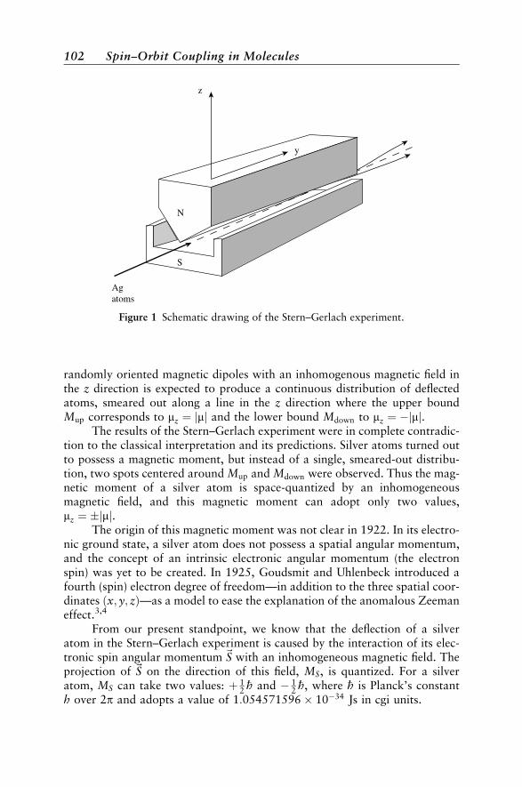
randomly oriented magnetic dipoles with an inhomogenous magnetic field inthe z direction is expected to produce a continuous distribution of deflectedatoms, smeared out along a line in the z direction where the upper boundMup corresponds to mz ¼ jmj and the lower bound Mdown to mz ¼ jmj.

The results of the Stern–Gerlach experiment were in complete contradic-tion to the classical interpretation and its predictions. Silver atoms turned outto possess a magnetic moment, but instead of a single, smeared-out distribu-tion, two spots centered around Mup and Mdown were observed. Thus the mag-netic moment of a silver atom is space-quantized by an inhomogeneousmagnetic field, and this magnetic moment can adopt only two values,mz ¼ jmj.

The origin of this magnetic moment was not clear in 1922. In its electro-nic ground state, a silver atom does not possess a spatial angular momentum,and the concept of an intrinsic electronic angular momentum (the electronspin) was yet to be created. In 1925, Goudsmit and Uhlenbeck introduced afourth (spin) electron degree of freedom—in addition to the three spatial coor-dinates ðx; y; zÞ—as a model to ease the explanation of the anomalous Zeemaneffect.3,4

From our present standpoint, we know that the deflection of a silveratom in the Stern–Gerlach experiment is caused by the interaction of its elec-tronic spin angular momentum ~S with an inhomogeneous magnetic field. Theprojection of ~S on the direction of this field, MS, is quantized. For a silveratom, MS can take two values: þ 1

2 h and 12 h, where h is Planck’s constant

h over 2p and adopts a value of 1:054571596 1034 Js in cgi units.

N

S

Agatoms

z

y

Figure 1 Schematic drawing of the Stern–Gerlach experiment.

102 Spin–Orbit Coupling in Molecules

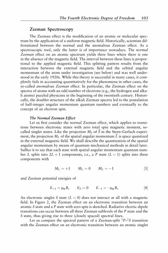
Zeeman Spectroscopy

The Zeeman effect is the modification of an atomic or molecular spec-trum by the application of a uniform magnetic field. Historically, scientists dif-ferentiated between the normal and the anomalous Zeeman effect. As aspectroscopic tool, only the latter is of importance nowadays. The normalZeeman effect on an atomic spectrum yields three lines where there is onein the absence of the magnetic field. The interval between these lines is propor-tional to the applied magnetic field. This splitting pattern results from theinteraction between the external magnetic field and the orbital angularmomentum of the atom under investigation (see below) and was well under-stood in the early 1920s. While this theory is successful in many cases, it com-pletely fails in accounting quantitatively for the phenomena in other cases, theso-called anomalous Zeeman effect. In particular, the Zeeman effect on thespectra of atoms with an odd number of electrons (e.g., the hydrogen and alka-li atoms) puzzled physicists in the beginning of the twentieth century. Histori-cally, the doublet structure of the alkali Zeeman spectra led to the postulationof half-integer angular momentum quantum numbers and eventually to theconcept of an electron spin.

The Normal Zeeman EffectLet us first consider the normal Zeeman effect, which applies to transi-

tions between electronic states with zero total spin magnetic moment, so-called singlet states. Like the projection MS of ~S in the Stern–Gerlach experi-ment, the projection ML of the spatial angular momentum ~L is space quantizedin the external magnetic field. We shall describe the quantization of the spatialangular momentum by means of quantum mechanical methods in detail later.Suffice it to say that each state with spatial angular momentum quantum num-ber L splits into 2Lþ 1 components, i.e., a P state (L ¼ 1) splits into threecomponents with

ML ¼ þ1 ML ¼ 0 ML ¼ 1 ½3

and Zeeman potential energies of

Eþ1 ¼ mB Bz E0 ¼ 0 E1 ¼ mB Bz ½4

An electronic singlet S state (L ¼ 0) does not interact at all with a magneticfield. In Figure 2, the Zeeman effect on an electronic transition between anatomic S state and a P state with zero spin is sketched. Radiative electric dipoletransitions can occur between all three Zeeman sublevels of the P state and theS state, thus giving rise to three (closely spaced) spectral lines.

Let us compare the spectral pattern of a Zeeman-split 1P–1S transitionwith the Zeeman effect on an electronic transition between an atomic singlet

The Fourth Electronic Degree of Freedom 103

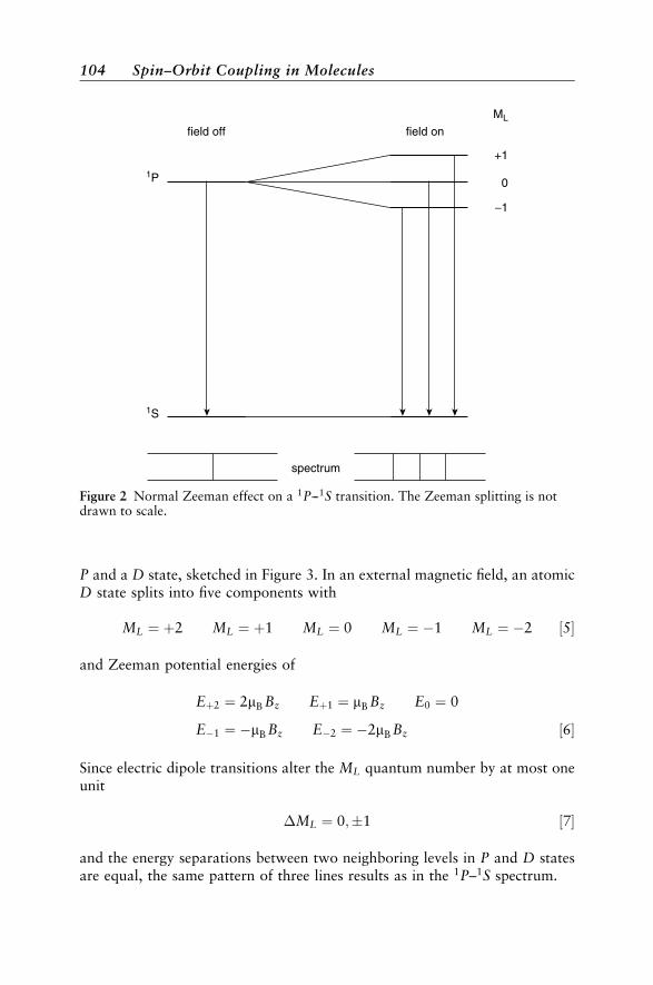
P and a D state, sketched in Figure 3. In an external magnetic field, an atomicD state splits into five components with

ML ¼ þ2 ML ¼ þ1 ML ¼ 0 ML ¼ 1 ML ¼ 2 ½5

and Zeeman potential energies of

Eþ2 ¼ 2mB Bz Eþ1 ¼ mB Bz E0 ¼ 0

E1 ¼ mB Bz E2 ¼ 2mB Bz ½6

Since electric dipole transitions alter the ML quantum number by at most oneunit

ML ¼ 0;1 ½7

and the energy separations between two neighboring levels in P and D statesare equal, the same pattern of three lines results as in the 1P–1S spectrum.

+1

0

−1

spectrum

field off field on

ML

1P

1S

Figure 2 Normal Zeeman effect on a 1P---1S transition. The Zeeman splitting is notdrawn to scale.

104 Spin–Orbit Coupling in Molecules

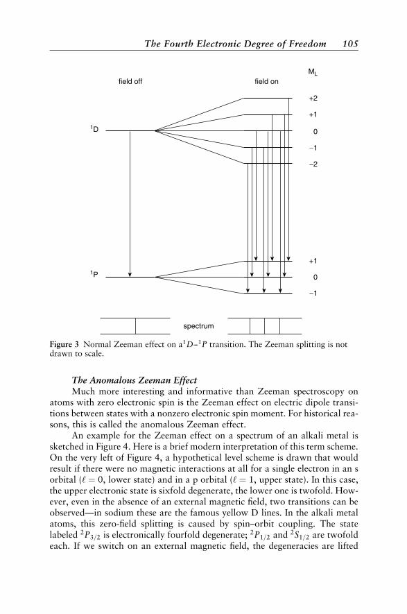
The Anomalous Zeeman EffectMuch more interesting and informative than Zeeman spectroscopy on

atoms with zero electronic spin is the Zeeman effect on electric dipole transi-tions between states with a nonzero electronic spin moment. For historical rea-sons, this is called the anomalous Zeeman effect.

An example for the Zeeman effect on a spectrum of an alkali metal issketched in Figure 4. Here is a brief modern interpretation of this term scheme.On the very left of Figure 4, a hypothetical level scheme is drawn that wouldresult if there were no magnetic interactions at all for a single electron in an sorbital (‘ ¼ 0, lower state) and in a p orbital (‘ ¼ 1, upper state). In this case,the upper electronic state is sixfold degenerate, the lower one is twofold. How-ever, even in the absence of an external magnetic field, two transitions can beobserved—in sodium these are the famous yellow D lines. In the alkali metalatoms, this zero-field splitting is caused by spin–orbit coupling. The statelabeled 2P3=2 is electronically fourfold degenerate; 2P1=2 and 2S1=2 are twofoldeach. If we switch on an external magnetic field, the degeneracies are lifted

field off field onML

spectrum

1D

1P 0

+1

0

−1

−2

+2

+1

−1

Figure 3 Normal Zeeman effect on a1D---1P transition. The Zeeman splitting is notdrawn to scale.

The Fourth Electronic Degree of Freedom 105

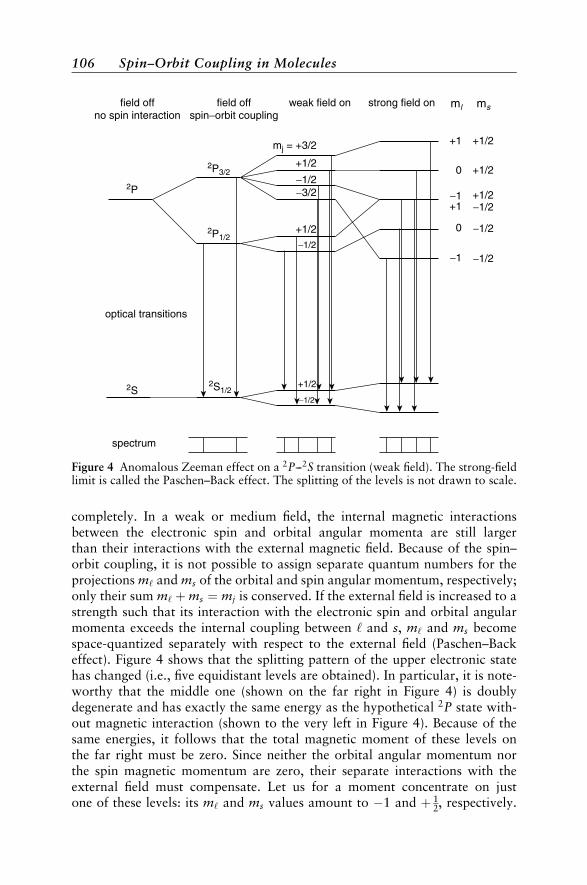
completely. In a weak or medium field, the internal magnetic interactionsbetween the electronic spin and orbital angular momenta are still largerthan their interactions with the external magnetic field. Because of the spin–orbit coupling, it is not possible to assign separate quantum numbers for theprojections m‘ and ms of the orbital and spin angular momentum, respectively;only their sum m‘ þms ¼ mj is conserved. If the external field is increased to astrength such that its interaction with the electronic spin and orbital angularmomenta exceeds the internal coupling between ‘ and s, m‘ and ms becomespace-quantized separately with respect to the external field (Paschen–Backeffect). Figure 4 shows that the splitting pattern of the upper electronic statehas changed (i.e., five equidistant levels are obtained). In particular, it is note-worthy that the middle one (shown on the far right in Figure 4) is doublydegenerate and has exactly the same energy as the hypothetical 2P state with-out magnetic interaction (shown to the very left in Figure 4). Because of thesame energies, it follows that the total magnetic moment of these levels onthe far right must be zero. Since neither the orbital angular momentum northe spin magnetic momentum are zero, their separate interactions with theexternal field must compensate. Let us for a moment concentrate on justone of these levels: its m‘ and ms values amount to 1 and þ 1

2, respectively.

spectrum

2S

2P

2P3/2

2P1/2

2S1/2

−1/2

−1/2

−1/2

optical transitions

−3/2−1/2

−1/2

−1/2

+1/2

mj = +3/2

+1/2

+1/2

+1/2

−1

+1

0

−1

+1/2

+1/2

0

+1

field offspin−orbit coupling

weak field on strong field onfield offno spin interaction

ml ms

Figure 4 Anomalous Zeeman effect on a 2P---2S transition (weak field). The strong-fieldlimit is called the Paschen–Back effect. The splitting of the levels is not drawn to scale.

106 Spin–Orbit Coupling in Molecules

For their interactions with the external field to be equal, the proportionalityconstant between the spin angular momentum and the associated magneticmoment must be twice as large as for the angular momentum. More precisely,this ratio amounts to 2.0023; the deviation from the value of 2, predicted byDirac theory, is mainly caused by radiative corrections explainable in theframework of quantum field theory.

Now, let us forget about spin and go back in history again. In 1921,Lande had been successful in deducing the energy separations of the atomicterm levels from the complicated splitting of spectral lines.6–8 The most funda-mental of his results was that he introduced half-integer magnetic quantumnumbers for the description of the doublet structure of the alkali spectra.[An integer value of the angular momentum quantum number j always givesrise to an odd number of Zeeman sublevels (2jþ 1); since the electronic statesof the alkali atoms split into an even number of sublevels, a half-integer valuehas to be postulated for j.] Even though it had become possible then todescribe the observed phenomena by means of mathematical formulas, theywere far from understood. At the beginning of the twentieth century, it wasgenerally believed that the doublet splitting had its origin in a nonzero angularmomentum of the nucleus. Indeed, the natural isotope of the Na nucleus has anonzero angular momentum (i.e., a nuclear spin I ¼ 3

2), which gives rise to anuclear Zeeman effect. This splitting is much smaller, by a factor of about2000, than the effect discussed here. It was Pauli who postulated in 1925that the anomalous Zeeman effect in the spectra of alkali atoms was solelydue to the valence electron and a strange, classically not describable ambiguityof its quantum theoretical properties:9

‘‘Die abgeschlossenen Elektronenkonfigurationen sollennichts zum magnetischen Moment und zum Impulsmomentdes Atoms beitragen. Insbesondere werden bei den Alkaliendie Impulswerte des Atoms und seine Energieanderungen ineinem außeren Magnetfeld im wesentlichen als eine alleinigeWirkung des Leuchtelektrons angesehen, das auch als der Sitzder magneto-mechanischen Anomalie betrachtet wird. DieDublettstruktur der Alkalispektren, sowie die Durchbrechungdes Larmortheorems kommt gemaß diesem Standpunkt durcheine eigentumliche, klassisch nicht beschreibbare Art vonZweideutigkeit der quantentheoretischen Eigenschaften desLeuchtelektrons zustande.’’a

aEnglish translation: The closed electron configurations shall not contribute to the magneticmoment and to the linear momentum of the atom. In particular, the (angular) momentumvalues of the alkali atoms and the changes of the atomic energies in an external magneticfield are regarded to be essentially solely due to the ‘‘Leuchtelekton’’ (valence electron),which is considered to be also the origin of the magnetomechanic anomaly. According to thisview, the doublet structure of the alkali spectra as well as the violation of the Larmortheorem is caused by a strange, classically not describable kind of ambiguity in the quantumtheoretical properties of the valence electron.

The Fourth Electronic Degree of Freedom 107

Carrying on the investigation of the anomalous Zeeman effect and thePaschen–Back effect on the spectra of the alkali atoms, Pauli postulated thatan electron in an external magnetic field has to be described by four indepen-dent quantum numbers. Moreover, in order to justify the Bohr–SommerfeldAufbau (building-up) principle of the periodic system of the elements, hecame up with his famous exclusion principle (Ausschließungsprinzip). In itsoriginal formulation it reads:10

‘‘Es kann niemals zwei oder mehrere aquivalente Elektronenim Atom geben, fur welche in starken Feldern die Werte allerQuantenzahlen n, k1, k2, m1 (oder, was dasselbe ist, n, k1,m1, m2) ubereinstimmen. Ist ein Elektron in Atom vorhan-den, fur das diese Quantenzahlen (im außeren Felde) be-stimmte Werte haben, so ist dieser Zustand ‘besetzt’ ’’.b

The four quantum numbers n, k1, k2, m1 are related to the quantum numbersin our modern terminology, that is, n (principal quantum number), ‘ (orbitalangular momentum), j (total angular momentum of an electron), and mj (pro-jection of j on the quantization axis), by

n ¼ n k1 ¼ ‘þ 1 k2 ¼ jþ 1

2m1 ¼ mj ½8

The postulate of a fourth independent quantum number was difficult to under-stand, since electrons were assumed to have only three—the spatial—degreesof freedom.

Shortly after the formulation of the exclusion principle, Goudsmit andUhlenbeck elegantly interpreted Pauli’s fourth independent electronic quan-tum number by postulating a fourth (spin) electron degree of freedom, anintrinsic angular momentum that is quantized and can adopt two orientationsin an external magnetic field.3,4 Assuming that the spin quantum number s ofan electron is 1

2 and that the ratio of the spin magnetic moment and the spinangular momentum is twice as large as for the orbital angular momentum, theanomalous Zeeman effect of the alkali atoms is easily explained.

Spin Is a Quantum Effect

Although the electron spin is often referred to as an intrinsic angularmomentum, it should be emphasized that spin has no classical analog. In par-ticular, one should not imagine a spinning electron as a particle rotating aboutan inner axis (e.g., like the earth does). Spin has to be regarded as a pure

bEnglish translation: There are never two or more electrons in an atom for which, in strongfields, the values of all quantum numbers n; k1; k2; m1 (or equivalently n; k1; m1; m2)agree. If in an atom an electron exists for which these quantum numbers (in an external field)have definite values, then this state is ‘‘occupied.’’

108 Spin–Orbit Coupling in Molecules

quantum effect. Sometimes we may try to simplify the description of its inter-actions by using the classical picture of a bar magnet, but we have to keep inmind that the rigorous treatment requires (relativistic) quantum theory. Con-trary to what we find in many textbooks, electron spin does not automaticallyfollow from relativistic invariance. Particles with different spin (0, 1

2, 1, 32, etc.)

are described by different relativistic equations. A proper (and the most com-mon) relativistic equation for a spin 1

2 particles is the Dirac equation.11 Themost compelling definition, at least known to the author, for the spin of a par-ticle with rest mass m 6¼ 0 is the following:12

Spin is the angular momentum of a particle at rest.

ANGULAR MOMENTA

Orbital Angular Momentum

Relation to an Infinitesimal RotationImagine a particle with position vector ~ra in a three-dimensional (3D)

orthonormal coordinate system with axes ~x, ~y, ~z and a wave functionð~raÞ ¼ ðxa; ya; zaÞ. If the particle is rotated about one of the axes ~x, ~y, or~z through an infinitesimal angle dj, the new position coordinates~r 0a are givenin first order by

x axis: x0a ¼ xa y0a ¼ ya djxza z0a ¼ za þ djxya

y axis: x0a ¼ xa þ djyza y0a ¼ ya z0a ¼ za djyxa

z axis: x0a ¼ xa djzya y0a ¼ ya þ djzxa z0a ¼ za

½9

To arrive at these equations, we have made use of the addition rules for thetrigonometric functions and have set cosðdjÞ 1 and sinðdjÞ dj. Anexample for a rotation about the z axis is shown in Figure 5. This result canbe generalized, if we interpret djx, djy, and djz as the components of an infi-nitesimal rotation vector ~dj. As indicated in Figure 6, ~dj points in the direc-tion of the rotation axis; its length is equal to the angle dj. Now, making useof the definition of the cross (vector) product, we can write the x component ofthe new position vector as

x0a ¼ xa þ djyza djzya ¼ xa þ ~dj~ra

x

½10

Similar relations are obtained for y0a and z0a. Thus, if the particle with positionvector~ra is rotated about a general axis through dj, its new position coordi-nates are given by

~r 0a ¼~ra þ d~ra ¼~ra þ ~dj~ra ½11

Angular Momenta 109

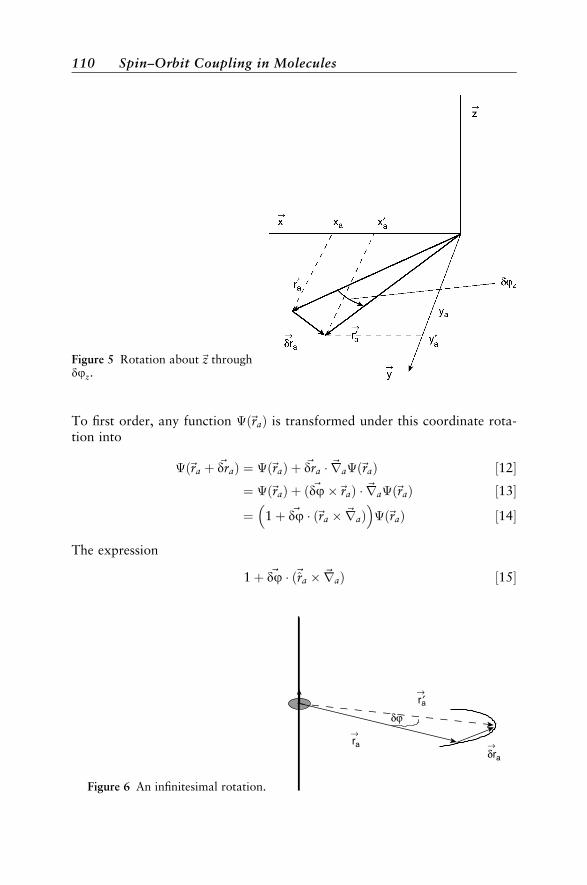
To first order, any function ð~raÞ is transformed under this coordinate rota-tion into

ð~ra þ ~draÞ ¼ ð~raÞ þ ~dra ~rað~raÞ ½12¼ ð~raÞ þ ð ~dj~raÞ ~rað~raÞ ½13

¼ 1þ ~dj ð~ra ~raÞ

ð~raÞ ½14

The expression

1þ ~dj ð~ra ~raÞ ½15

Figure 5 Rotation about~z throughdjz.

ra

r ′

δra

δϕ→

→

→

a

Figure 6 An infinitesimal rotation.

110 Spin–Orbit Coupling in Molecules

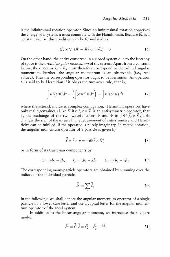
is the infinitesimal rotation operator. Since an infinitesimal rotation conservesthe energy of a system, it must commute with the Hamiltonian. Because ~dj is aconstant vector, this condition can be formulated as

ð~ra ~raÞH Hð~ra ~raÞ ¼ 0 ½16

On the other hand, the entity conserved in a closed system due to the isotropyof space is the orbital angular momentum of the system. Apart from a constantfactor, the operator ~ra ~ra must therefore correspond to the orbital angularmomentum. Further, the angular momentum is an observable (i.e., realvalued). Thus the corresponding operator ought to be Hermitian. An operatorO is said to be Hermitian if it obeys the turn-over rule, that is,

ððOÞdt ¼

ððOÞdt

¼ððOÞdt ½17

where the asterisk indicates complex conjugation. (Hermitian operators haveonly real eigenvalues.) Like ~r itself, ~r ~r is an antisymmetric operator, thatis, the exchange of the two wavefunctions and in

Ðð~ra ~raÞdt

changes the sign of the integral. The requirement of antisymmetry and Hermi-ticity can be fulfilled, if the operator is purely imaginary. In vector notation,the angular momentum operator of a particle is given by

~‘ ¼ ~r ~p ¼ ihð~r ~rÞ ½18

or in form of its Cartesian components by

‘x ¼ ypz zpy ‘y ¼ zpx xpz ‘z ¼ xpy ypx ½19

The corresponding many-particle operators are obtained by summing over theindices of the individual particles

~L ¼

Xa

~‘a ½20

In the following, we shall denote the angular momentum operator of a singleparticle by a lower case letter and use a capital letter for the angular momen-tum operator of the total system.

In addition to the linear angular momenta, we introduce their squaremoduli

‘2 ¼ ~‘ ~‘ ¼ ‘2

x þ ‘2y þ ‘2

z ½21

Angular Momenta 111

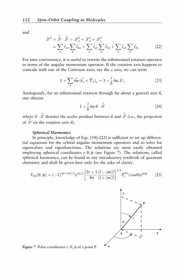
and

L2 ¼ ~L ~L ¼ L2

x þ L2y þ L2

z

¼X

a

‘ax

Xb

‘bx þX

a

‘ay

Xb

‘by þX

a

‘az

Xb

‘bz ½22

For later convenience, it is useful to rewrite the infinitesimal rotation operatorin terms of the angular momentum operator. If the rotation axis happens tocoincide with one of the Cartesian axes, say the z axis, we can write

1þX

a

~dj ð~ra ~raÞz ¼ 1þ i

hdj Lz ½23

Analogously, for an infinitesimal rotation through dj about a general axis ~n,one obtains

1þ i

hdj~n ~L ½24

where ~n ~L denotes the scalar product between ~n and ~L (i.e., the projection

of ~L on the rotation axis ~n).

Spherical HarmonicsIn principle, knowledge of Eqs. [18]–[22] is sufficient to set up differen-

tial equations for the orbital angular momentum operators and to solve foreigenvalues and eigenfunctions. The solutions are most easily obtainedemploying spherical coordinates r; y;f (see Figure 7). The solutions, calledspherical harmonics, can be found in any introductory textbook of quantumchemistry and shall be given here only for the sake of clarity.

Y‘mðy;fÞ ¼ ð1ÞðmþjmjÞ=2ei‘p=2 2‘þ 1

4pðl jmjÞ!ðl þ jmjÞ!

1=2

Pjmj‘ ðcosyÞeimf ½25

x

y

z

P

rθ

φ

o

Figure 7 Polar coordinates r, y, f of a point P.

112 Spin–Orbit Coupling in Molecules

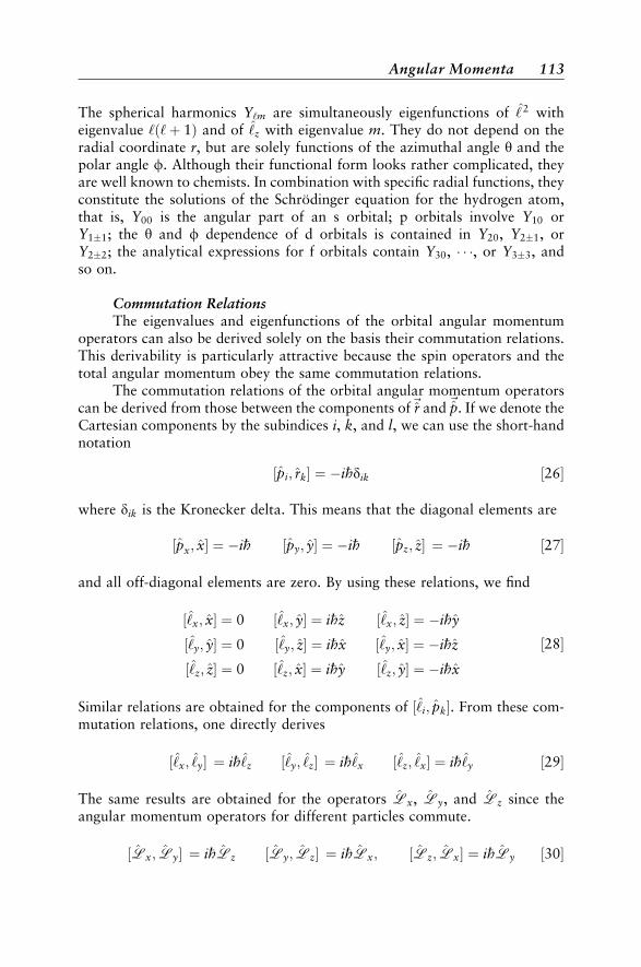
The spherical harmonics Y‘m are simultaneously eigenfunctions of ‘2 witheigenvalue ‘ð‘þ 1Þ and of ‘z with eigenvalue m. They do not depend on theradial coordinate r, but are solely functions of the azimuthal angle y and thepolar angle f. Although their functional form looks rather complicated, theyare well known to chemists. In combination with specific radial functions, theyconstitute the solutions of the Schrodinger equation for the hydrogen atom,that is, Y00 is the angular part of an s orbital; p orbitals involve Y10 orY11; the y and f dependence of d orbitals is contained in Y20, Y21, orY22; the analytical expressions for f orbitals contain Y30, , or Y33, andso on.

Commutation RelationsThe eigenvalues and eigenfunctions of the orbital angular momentum

operators can also be derived solely on the basis their commutation relations.This derivability is particularly attractive because the spin operators and thetotal angular momentum obey the same commutation relations.

The commutation relations of the orbital angular momentum operatorscan be derived from those between the components of~r and ~p. If we denote theCartesian components by the subindices i, k, and l, we can use the short-handnotation

½pi; rk ¼ ihdik ½26

where dik is the Kronecker delta. This means that the diagonal elements are

½px; x ¼ ih ½py; y ¼ ih ½pz; z ¼ ih ½27

and all off-diagonal elements are zero. By using these relations, we find

½‘x; x ¼ 0 ½‘x; y ¼ ihz ½‘x; z ¼ ihy

½‘y; y ¼ 0 ½‘y; z ¼ ihx ½‘y; x ¼ ihz

½‘z; z ¼ 0 ½‘z; x ¼ ihy ½‘z; y ¼ ihx

½28

Similar relations are obtained for the components of ½‘i; pk. From these com-mutation relations, one directly derives

½‘x; ‘y ¼ ih‘z ½‘y; ‘z ¼ ih‘x ½‘z; ‘x ¼ ih‘y ½29

The same results are obtained for the operators Lx, Ly, and Lz since theangular momentum operators for different particles commute.

½Lx; Ly ¼ ihLz ½Ly; Lz ¼ ihLx; ½Lz; Lx ¼ ihLy ½30

Angular Momenta 113

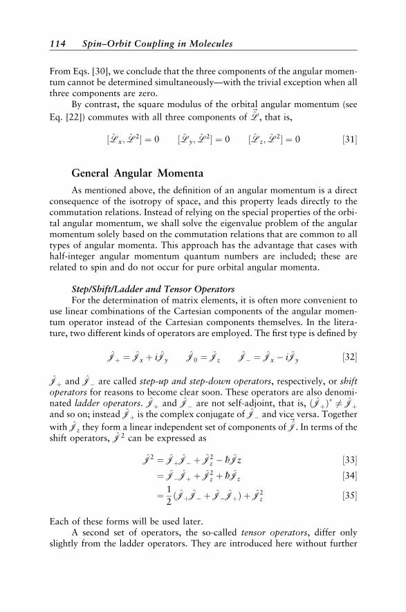
From Eqs. [30], we conclude that the three components of the angular momen-tum cannot be determined simultaneously—with the trivial exception when allthree components are zero.

By contrast, the square modulus of the orbital angular momentum (see

Eq. [22]) commutes with all three components of ~L, that is,

½Lx; L2 ¼ 0 ½Ly; L

2 ¼ 0 ½Lz; L2 ¼ 0 ½31

General Angular Momenta

As mentioned above, the definition of an angular momentum is a directconsequence of the isotropy of space, and this property leads directly to thecommutation relations. Instead of relying on the special properties of the orbi-tal angular momentum, we shall solve the eigenvalue problem of the angularmomentum solely based on the commutation relations that are common to alltypes of angular momenta. This approach has the advantage that cases withhalf-integer angular momentum quantum numbers are included; these arerelated to spin and do not occur for pure orbital angular momenta.

Step/Shift/Ladder and Tensor OperatorsFor the determination of matrix elements, it is often more convenient to

use linear combinations of the Cartesian components of the angular momen-tum operator instead of the Cartesian components themselves. In the litera-ture, two different kinds of operators are employed. The first type is defined by

Jþ ¼ Jx þ iJy J0 ¼ Jz J ¼ Jx iJy ½32

Jþ and J are called step-up and step-down operators, respectively, or shiftoperators for reasons to become clear soon. These operators are also denomi-nated ladder operators. Jþ and J are not self-adjoint, that is, ðJþÞ

6¼ Jþand so on; instead Jþ is the complex conjugate of J and vice versa. Together

with Jz they form a linear independent set of components of~J. In terms of the

shift operators, J2 can be expressed as

J2 ¼ JþJ þJ2z hJz ½33

¼ JJþ þJ2z þ hJz ½34

¼ 1

2ðJþJ þJJþÞ þJ2

z ½35

Each of these forms will be used later.A second set of operators, the so-called tensor operators, differ only

slightly from the ladder operators. They are introduced here without further

114 Spin–Orbit Coupling in Molecules

explanation. Cartesian and spherical tensor components are related by

Jþ1 ¼ Jx þ iJyffiffiffi

2p J0 ¼ Jz J1 ¼

Jx iJyffiffiffi2p ½36

or conversely

Jx ¼J1 Jþ1ffiffiffi

2p Jz ¼ J0 Jy ¼

iðJ1 þJþ1Þffiffiffi2p ½37

Phase conventions have been chosen to be consistent with those of Condon

and Shortley.13 In terms of tensor operators, the square modulus of~J becomes

J2 ¼ Jþ1J1 J1Jþ1 þJ20 ½38

We shall come back to these operators after learning what a tensor is.

Commutation RelationsAs for the orbital angular momentum, the commutation relations

between the Cartesian components of a general angular momentum~J and

its square modulus J2 read

½Jx;Jy ¼ ihJz ½Jy;Jz ¼ ihJx ½Jz;Jx ¼ ihJy ½39

and

½Jx;J2 ¼ 0 ½Jy;J

2 ¼ 0 ½Jz;J2 ¼ 0 ½40

Using Eq. [39] and the definition of the step-up and step-down operators(Eq. [32]), one easily obtains their commutation relations

½Jþ;J ¼ 2hJz ½41

and

½Jz;J ¼ hJ ½42

From the latter, the useful relation

½Jz;Jn ¼ nhJ ½43

can be derived.

Angular Momenta 115

Like the Cartesian components, the shift operators also commute withJ2

½J;J2 ¼ 0 ½44

The same is true for the tensor operators.

½J1;J2 ¼ 0 ½45

The commutation relations among their components differ slightly from thoseof the shift operators. From Eqs. [36] and [39], it follows that

½Jþ1;J1 ¼ hJ0 ½46

and

½J0;J1 ¼ hJ1 ½47

The Eigenvalues of J2 and Jz

Because J2 and Jz commute, they must have common eigenvectors thatwe shall denote by jui. The eigenvectors satisfy the equations

J2jui ¼ ah2jui ½48Jzjui ¼Mhjui ½49

Applying Eqs. [42] to the eigenvectors jui

JzJjui ¼ JJzjui hJjui ¼ ðM 1ÞhJjui ½50

we see that Jjui are also eigenvectors of Jz, but with eigenvalue ðM 1Þh.

Moreover, Jjui is also an eigenvector of J2 with eigenvalue ah2 because

J2Jjui ¼ JJ2jui ¼ ah2

Jjui ½51

This means that the action of Jþ on an eigenvector of Jz and J2 is to step upthe eigenvalue of Jz by one unit while remaining within the subset of functionsbelonging to the eigenvalue a of J2. J analogously steps down the eigenvalueof Jz by one unit.

To set up a connection between a and M, we express J2 in the form Eq.[35] and note that Jþ and J are Hermitian conjugates. Applying the turn-over rule (Eq. [17]) yields

hJfjJfi ¼ 1

2hJfjJfi þ

1

2hJþfjJþfi þ hJzfjJzfi ½52

116 Spin–Orbit Coupling in Molecules

Each of these terms is always positive or zero—this follows from the fact thatthe length of a vector is always positive or zero. The fact that each of the termsin Eq. [52] is positive or zero leads us to the inequality

hfjJ2jfi hfjJ2z jfi 0 ½53

By identifying jfi with an eigenvector jui, we obtain from Eqs. [48] and [49]

a M2 0 ½54a

or

ffiffiffiapM

ffiffiffiap

½54b

which means that the eigenvalues M are limited from above and below; thereis a minimal value Mmin and a maximal value Mmax.

In particular, if we apply Eq. [50] to an eigenvector jumaxi belonging toMmax

JzJþjumaxi ¼ ðMmax þ 1ÞhJþjumaxi ½56

then this equation can only be satisfied, if

Jþjumaxi ¼ 0 ½57

because Mmax was assumed to be the maximal M value. Using expression [34]yields

JJþjumaxi ¼ ðJ2 J2z hJzÞjumaxi ¼ 0 ½58

leading to

ah2 M2max h

2 Mmaxh2 ¼ 0 ½59

From this, we obtain the relation between a and Mmax

a ¼MmaxðMmax þ 1Þ ½60

Analogously, application of expression [33] to jumini yields

a ¼MminðMmin 1Þ ½61

Angular Momenta 117

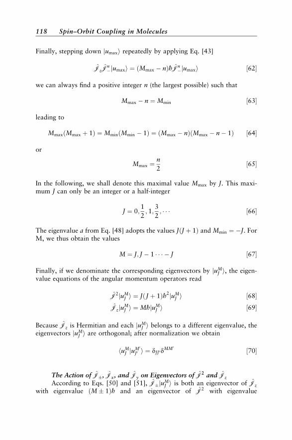
Finally, stepping down jumaxi repeatedly by applying Eq. [43]

JzJnjumaxi ¼ ðMmax nÞhJn

jumaxi ½62

we can always find a positive integer n (the largest possible) such that

Mmax n ¼Mmin ½63

leading to

MmaxðMmax þ 1Þ ¼MminðMmin 1Þ ¼ ðMmax nÞðMmax n 1Þ ½64

or

Mmax ¼n

2½65

In the following, we shall denote this maximal value Mmax by J. This maxi-mum J can only be an integer or a half-integer

J ¼ 0;1

2; 1;

3

2; ½66

The eigenvalue a from Eq. [48] adopts the values JðJ þ 1Þ and Mmin ¼ J. ForM, we thus obtain the values

M ¼ J; J 1 J ½67

Finally, if we denominate the corresponding eigenvectors by juMJ i, the eigen-

value equations of the angular momentum operators read

J2juMJ i ¼ JðJ þ 1Þh2juM

J i ½68JzjuM

J i ¼MhjuMJ i ½69

Because Jz is Hermitian and each juMJ i belongs to a different eigenvalue, the

eigenvectors juMJ i are orthogonal; after normalization we obtain

huMJ juM0

J0 i ¼ dJJ0dMM0 ½70

The Action of J, Jx, and Jy on Eigenvectors of J2 and Jz

According to Eqs. [50] and [51], JjuMJ i is both an eigenvector of Jz

with eigenvalue ðM 1Þh and an eigenvector of J2 with eigenvalue

118 Spin–Orbit Coupling in Molecules

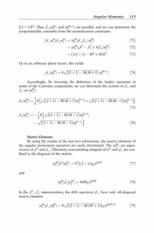
JðJ þ 1Þh2. Thus JjuMJ i and juM1

J i are parallel, and we can determine theproportionality constants from the normalization constraint:

hJuMJ jJuM

J i ¼ huMJ jJJ juM

J i ½71

¼ huMJ jðJ2 J2

z hJzÞjuMJ i ½72

¼ JðJ þ 1Þ M2 M

h2 ½73

Up to an arbitrary phase factor, this yields

JjuMJ i ¼ h

ffiffiffiffiffiffiffiffiffiffiffiffiffiffiffiffiffiffiffiffiffiffiffiffiffiffiffiffiffiffiffiffiffiffiffiffiffiffiffiffiffiffiffiffiJðJ þ 1Þ MðM 1Þ

pjuM1

J i ½74

Accordingly, by inverting the definition of the ladder operators interms of the Cartesian components, we can determine the actions of Jx andJy on juM

J i:

JxjuMJ i ¼

1

2h

ffiffiffiffiffiffiffiffiffiffiffiffiffiffiffiffiffiffiffiffiffiffiffiffiffiffiffiffiffiffiffiffiffiffiffiffiffiffiffiffiffiffiffiffiJðJ þ 1Þ MðMþ 1Þ

pjuMþ1

J in

þffiffiffiffiffiffiffiffiffiffiffiffiffiffiffiffiffiffiffiffiffiffiffiffiffiffiffiffiffiffiffiffiffiffiffiffiffiffiffiffiffiffiffiffiJðJ þ 1Þ MðM 1Þ

pjuM1

J io½75

JyjuMJ i ¼

i

2h

ffiffiffiffiffiffiffiffiffiffiffiffiffiffiffiffiffiffiffiffiffiffiffiffiffiffiffiffiffiffiffiffiffiffiffiffiffiffiffiffiffiffiffiffiJðJ þ 1Þ MðMþ 1Þ

pjuMþ1

J in

ffiffiffiffiffiffiffiffiffiffiffiffiffiffiffiffiffiffiffiffiffiffiffiffiffiffiffiffiffiffiffiffiffiffiffiffiffiffiffiffiffiffiffiffiJðJ þ 1Þ MðM 1Þ

pjuM1

J io

½76

Matrix ElementsBy using the results of the last two subsections, the matrix elements of

the angular momentum operators are easily determined. The juMJ i are eigen-

vectors of J2 and Jz. Therefore, nonvanishing integrals of J2 and Jz are con-fined to the diagonal of the matrix.

huMJ jJ2juM0

J0 i ¼ h2JðJ þ 1ÞdJJ0dMM0 ½77

and

huMJ jJzjuM0

J0 i ¼ hMdJJ0dMM0 ½78

In the J2, Jz representation, the shift operators J have only off-diagonalmatrix elements

huMJ jJjuM0

J0 i ¼ hffiffiffiffiffiffiffiffiffiffiffiffiffiffiffiffiffiffiffiffiffiffiffiffiffiffiffiffiffiffiffiffiffiffiffiffiffiffiffiffiffiffiffiffiffiffiJðJ þ 1Þ M0ðM0 1Þ

pdJJ0d

MM01 ½79

Angular Momenta 119

The same is true for the Cartesian Jx and Jy

huMJ jJxjuM0

J0 i ¼1

2hffiffiffiffiffiffiffiffiffiffiffiffiffiffiffiffiffiffiffiffiffiffiffiffiffiffiffiffiffiffiffiffiffiffiffiffiffiffiffiffiffiffiffiffiffiffiJðJ þ 1Þ M0ðM0 þ 1Þ

pdJJ0d

MM01

þ 1

2hffiffiffiffiffiffiffiffiffiffiffiffiffiffiffiffiffiffiffiffiffiffiffiffiffiffiffiffiffiffiffiffiffiffiffiffiffiffiffiffiffiffiffiffiffiffiJðJ þ 1Þ M0ðM0 1Þ

pdJJ0d

MM01 ½80

huMJ jJyjuM0

J0 i ¼ i

2hffiffiffiffiffiffiffiffiffiffiffiffiffiffiffiffiffiffiffiffiffiffiffiffiffiffiffiffiffiffiffiffiffiffiffiffiffiffiffiffiffiffiffiffiffiffiJðJ þ 1Þ M0ðM0 þ 1Þ

pdJJ0d

MM01

þ i

2hffiffiffiffiffiffiffiffiffiffiffiffiffiffiffiffiffiffiffiffiffiffiffiffiffiffiffiffiffiffiffiffiffiffiffiffiffiffiffiffiffiffiffiffiffiffiJðJ þ 1Þ M0ðM0 1Þ

pdJJ0d

MM01 ½81

In particular, for J ¼ 12 states we obtain

huMJ jJ2juM0

J i ¼

M M0 12 1

2

12

34 h

2 0

12 0 3

4 h2

½82

huMJ jJzjuM0

J i ¼

M M0 12 1

2

12

12 h 0

12 0 1

2 h

½83

huMJ jJþjuM0

J i ¼

M M0 12 1

2

12 0 h

12 0 0

½84

huMJ jJjuM0

J i ¼

M M0 12 1

2

12 0 0

12 h 0

½85

huMJ jJx juM0

J i ¼

M M0 12 1

2

12 0 1

2 h

12

12 h 0

½86

huMJ jJyjuM0

J i ¼

M M0 12 1

2

12 0 i

2 h

12

i2 h 0

½87

120 Spin–Orbit Coupling in Molecules

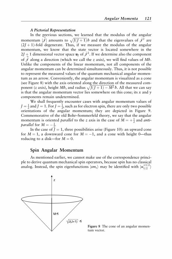
A Pictorial RepresentationIn the previous sections, we learned that the modulus of the angular

momentum j~Jj amounts toffiffiffiffiffiffiffiffiffiffiffiffiffiffiffiffiffiJðJ þ 1Þ

ph and that the eigenvalues of J2 are

ð2J þ 1Þ-fold degenerate. Thus, if we measure the modulus of the angularmomentum, we know that the state vector is located somewhere in the2J þ 1 dimensional vector space uJ of J2. If we determine also the component

of~J along a direction (which we call the z axis), we will find values of Mh.

Unlike the components of the linear momentum, not all components of theangular momentum can be determined simultaneously. Thus, it is not possibleto represent the measured values of the quantum mechanical angular momen-tum as an arrow. Conveniently, the angular momentum is visualized as a cone(see Figure 8) with the axis oriented along the direction of the measured com-ponent (z axis), height Mh, and radius

ffiffiffiffiffiffiffiffiffiffiffiffiffiffiffiffiffiffiffiffiffiffiffiffiffiffiffiffiffiffiJðJ þ 1Þ M2

ph. All that we can say

is that the angular momentum vector lies somewhere on this cone; its x and ycomponents remain undetermined.

We shall frequently encounter cases with angular momentum values ofJ ¼ 1

2 and J ¼ 1. For J ¼ 12, such as for electron spin, there are only two possible

orientations of the angular momentum; they are depicted in Figure 9.Commemorative of the old Bohr–Sommerfeld theory, we say that the angularmomentum is oriented parallel to the z axis in the case of M ¼ þ 1

2 and anti-parallel for M ¼ 1

2.In the case of J ¼ 1, three possibilities arise (Figure 10): an upward cone

for M ¼ 1, a downward cone for M ¼ 1, and a cone with height 0—thusreducing to a disk—for M ¼ 0.

Spin Angular Momentum

As mentioned earlier, we cannot make use of the correspondence princi-ple to derive quantum mechanical spin operators, because spin has no classicalanalog. Instead, the spin eigenfunctions jsmsi may be identified with ju1=2

1=2 i

J(J+1) h

M h

z

Figure 8 The cone of an angular momen-tum vector.

Angular Momenta 121

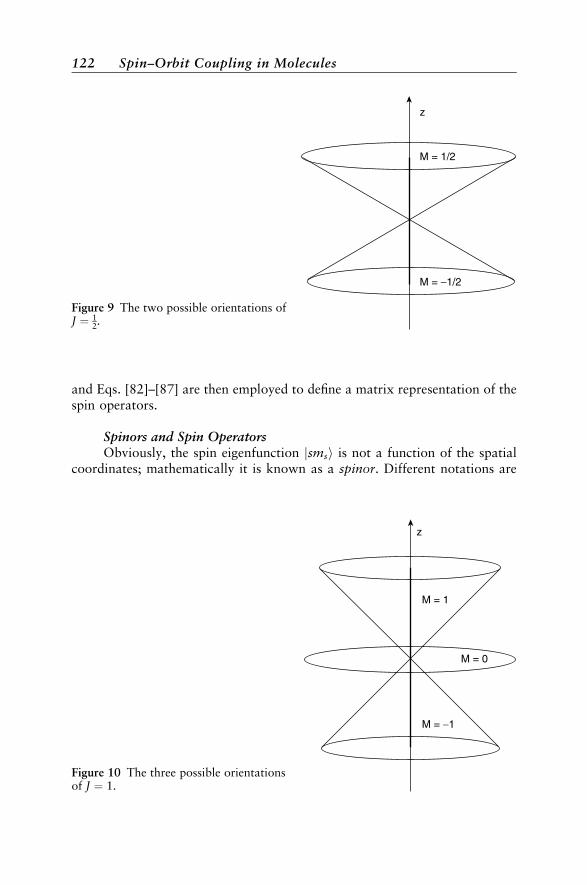
and Eqs. [82]–[87] are then employed to define a matrix representation of thespin operators.

Spinors and Spin OperatorsObviously, the spin eigenfunction jsmsi is not a function of the spatial

coordinates; mathematically it is known as a spinor. Different notations are

M = 1/2

z

M = −1/2

Figure 9 The two possible orientations ofJ ¼ 1

2.

z

M = 0

M = 1

M = −1

Figure 10 The three possible orientationsof J ¼ 1.

122 Spin–Orbit Coupling in Molecules

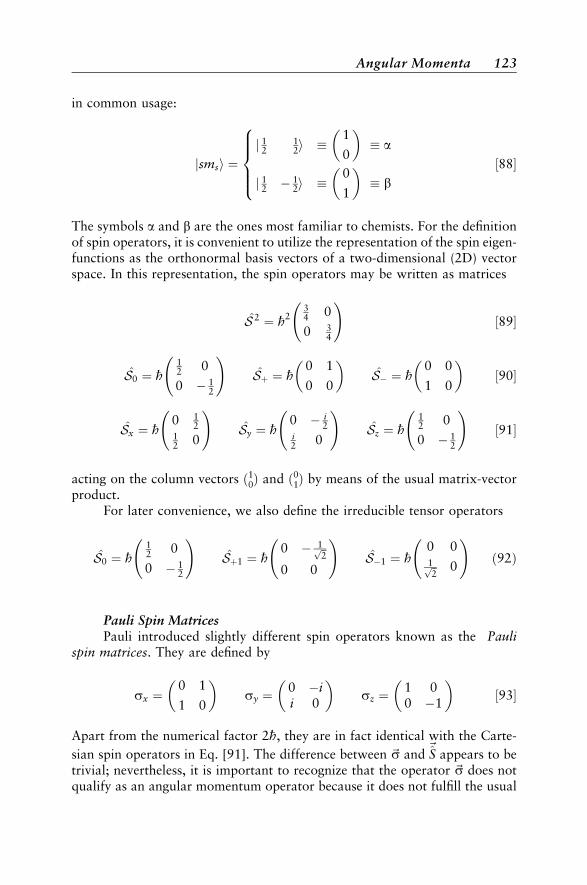
in common usage:

jsmsi ¼j 12 1

2i 1

0

a

j 12 12i

0

1

b

8>>><>>>: ½88

The symbols a and b are the ones most familiar to chemists. For the definitionof spin operators, it is convenient to utilize the representation of the spin eigen-functions as the orthonormal basis vectors of a two-dimensional (2D) vectorspace. In this representation, the spin operators may be written as matrices

S 2 ¼ h234 0

0 34

!½89

S0 ¼ h12 0

0 12

!Sþ ¼ h

0 1

0 0

S ¼ h

0 0

1 0

½90

Sx ¼ h0 1

212 0

!Sy ¼ h

0 i2

i2 0

!Sz ¼ h

12 0

0 12

!½91

acting on the column vectors ð10Þ and ð01Þ by means of the usual matrix-vectorproduct.

For later convenience, we also define the irreducible tensor operators

S0 ¼ h12 0

0 12

!Sþ1 ¼ h

0 1ffiffi2p

0 0

!S1 ¼ h

0 01ffiffi2p 0

!ð92Þ

Pauli Spin MatricesPauli introduced slightly different spin operators known as the Pauli

spin matrices. They are defined by

sx ¼0 1

1 0

sy ¼

0 ii 0

sz ¼

1 00 1

½93

Apart from the numerical factor 2h, they are in fact identical with the Carte-

sian spin operators in Eq. [91]. The difference between ~s and~S appears to be

trivial; nevertheless, it is important to recognize that the operator ~s does notqualify as an angular momentum operator because it does not fulfill the usual

Angular Momenta 123

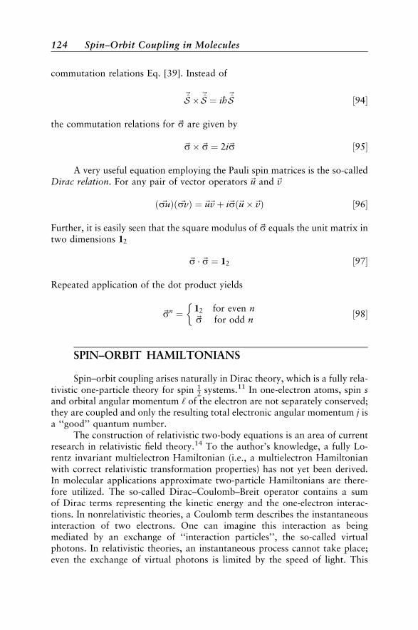
commutation relations Eq. [39]. Instead of

~S ~S ¼ ih~S ½94

the commutation relations for ~s are given by

~s~s ¼ 2i~s ½95

A very useful equation employing the Pauli spin matrices is the so-calledDirac relation. For any pair of vector operators ~u and ~v

ð ~suÞð ~svÞ ¼~u~vþ i~sð~u~vÞ ½96

Further, it is easily seen that the square modulus of ~s equals the unit matrix intwo dimensions 12

~s ~s ¼ 12 ½97

Repeated application of the dot product yields

~sn ¼ 12 for even n~s for odd n

½98

SPIN–ORBIT HAMILTONIANS

Spin–orbit coupling arises naturally in Dirac theory, which is a fully rela-tivistic one-particle theory for spin 1

2 systems.11 In one-electron atoms, spin sand orbital angular momentum ‘ of the electron are not separately conserved;they are coupled and only the resulting total electronic angular momentum j isa ‘‘good’’ quantum number.

The construction of relativistic two-body equations is an area of currentresearch in relativistic field theory.14 To the author’s knowledge, a fully Lo-rentz invariant multielectron Hamiltonian (i.e., a multielectron Hamiltonianwith correct relativistic transformation properties) has not yet been derived.In molecular applications approximate two-particle Hamiltonians are there-fore utilized. The so-called Dirac–Coulomb–Breit operator contains a sumof Dirac terms representing the kinetic energy and the one-electron interac-tions. In nonrelativistic theories, a Coulomb term describes the instantaneousinteraction of two electrons. One can imagine this interaction as beingmediated by an exchange of ‘‘interaction particles’’, the so-called virtualphotons. In relativistic theories, an instantaneous process cannot take place;even the exchange of virtual photons is limited by the speed of light. This

124 Spin–Orbit Coupling in Molecules

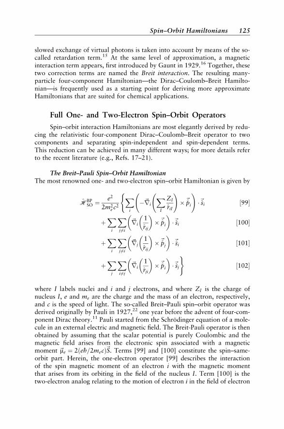
slowed exchange of virtual photons is taken into account by means of the so-called retardation term.15 At the same level of approximation, a magneticinteraction term appears, first introduced by Gaunt in 1929.16 Together, thesetwo correction terms are named the Breit interaction. The resulting many-particle four-component Hamiltonian—the Dirac–Coulomb–Breit Hamilto-nian—is frequently used as a starting point for deriving more approximateHamiltonians that are suited for chemical applications.

Full One- and Two-Electron Spin–Orbit Operators

Spin–orbit interaction Hamiltonians are most elegantly derived by redu-cing the relativistic four-component Dirac–Coulomb–Breit operator to twocomponents and separating spin-independent and spin-dependent terms.This reduction can be achieved in many different ways; for more details referto the recent literature (e.g., Refs. 17–21).

The Breit–Pauli Spin–Orbit HamiltonianThe most renowned one- and two-electron spin–orbit Hamiltonian is given by

HBPSO ¼

e2

2m2e c2

Xi

~ri

XI

ZI

riI

! ~pi

!~si

(½99

þX

i

Xj 6¼i

~ri1

rij

~pi

~si ½100

þX

i

Xj 6¼i

~rj1

rij

~pj

~si ½101

þX

j

Xi 6¼j

~ri1

rji

~pi

~sj

)½102

where I labels nuclei and i and j electrons, and where ZI is the charge ofnucleus I, e and me are the charge and the mass of an electron, respectively,and c is the speed of light. The so-called Breit–Pauli spin–orbit operator wasderived originally by Pauli in 1927,22 one year before the advent of four-com-ponent Dirac theory.11 Pauli started from the Schrodinger equation of a mole-cule in an external electric and magnetic field. The Breit-Pauli operator is thenobtained by assuming that the scalar potential is purely Coulombic and themagnetic field arises from the electronic spin associated with a magneticmoment ~me ¼ 2ðeh=2mecÞ~S. Terms [99] and [100] constitute the spin–same-orbit part. Herein, the one-electron operator [99] describes the interactionof the spin magnetic moment of an electron i with the magnetic momentthat arises from its orbiting in the field of the nucleus I. Term [100] is thetwo-electron analog relating to the motion of electron i in the field of electron

Spin–Orbit Hamiltonians 125

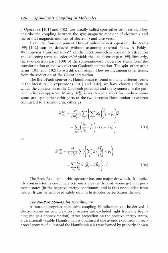
j. Operators [101] and [102] are usually called spin–other-orbit terms. Theydescribe the coupling between the spin magnetic moment of electron i andthe orbital magnetic moment of electron j and vice versa.

From the four-component Dirac–Coulomb–Breit equation, the terms[99]–[102] can be deduced without assuming external fields. A Foldy–Wouthuysen transformation23 of the electron-nuclear Coulomb attractionand collecting terms to order v2=c2 yields the one-electron part [99]. Similarly,the two-electron part [100] of the spin–same–orbit operator stems from thetransformation of the two-electron Coulomb interaction. The spin–other-orbitterms [101] and [102] have a different origin. They result, among other terms,from the reduction of the Gaunt interaction.

The Breit-Pauli spin–orbit Hamiltonian is found in many different formsin the literature. In expressions [101] and [102], we have chosen a form inwhich the connection to the Coulomb potential and the symmetry in the par-ticle indices is apparent. Mostly HBP

SO is written in a short form where spin–same- and spin–other-orbit parts of the two-electron Hamiltonian have beencontracted to a single term, either as

HBPSO ¼

e2

2m2e c2

Xi

XI

ZI

~riI

r3iI

~pi

!~si

(

Xj 6¼i

~rij

r3ij

~pi

! ð~si þ 2~sjÞ

)½103

or

HBPSO ¼

e2

2m2e c2

Xi

XI

ZI

~riI

r3iI

~pi

!(

Xj 6¼j

~rij

r3ij

ð~pi 2~pjÞ)~si ½104

The Breit-Pauli spin–orbit operator has one major drawback. It implic-itly contains terms coupling electronic states (with positive energy) and posi-tronic states (in the negative energy continuum) and is thus unbounded frombelow. It can be employed safely only in first-order perturbation theory.

The No-Pair Spin–Orbit HamiltonianA more appropriate spin–orbit coupling Hamiltonian can be derived if

electron–positron pair creation processes are excluded right from the begin-ning (no-pair approximation). After projection on the positive energy states,a variationally stable Hamiltonian is obtained if one avoids expansion in reci-procal powers of c. Instead the Hamiltonian is transformed by properly chosen

126 Spin–Orbit Coupling in Molecules

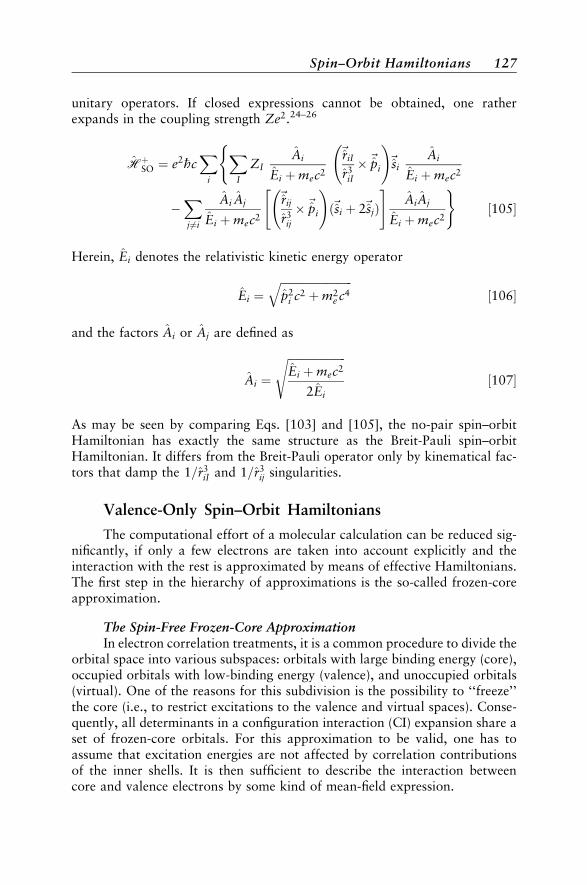
unitary operators. If closed expressions cannot be obtained, one ratherexpands in the coupling strength Ze2.24–26

HþSO ¼ e2hc

Xi

XI

ZIAi

Ei þmec2

~riI

r3iI

~pi

!~si

Ai

Ei þmec2

(

Xj6¼i

Ai Aj

Ei þmec2

~rij

r3ij

~pi

!ð~si þ 2~sjÞ

" #AiAj

Ei þmec2

)½105

Herein, Ei denotes the relativistic kinetic energy operator

Ei ¼ffiffiffiffiffiffiffiffiffiffiffiffiffiffiffiffiffiffiffiffiffiffiffiffiffiffip2

i c2 þm2e c4

q½106

and the factors Ai or Aj are defined as

Ai ¼

ffiffiffiffiffiffiffiffiffiffiffiffiffiffiffiffiffiffiffiffiffiEi þmec2

2Ei

s½107

As may be seen by comparing Eqs. [103] and [105], the no-pair spin–orbitHamiltonian has exactly the same structure as the Breit-Pauli spin–orbitHamiltonian. It differs from the Breit-Pauli operator only by kinematical fac-tors that damp the 1=r3

iI and 1=r3ij singularities.

Valence-Only Spin–Orbit Hamiltonians

The computational effort of a molecular calculation can be reduced sig-nificantly, if only a few electrons are taken into account explicitly and theinteraction with the rest is approximated by means of effective Hamiltonians.The first step in the hierarchy of approximations is the so-called frozen-coreapproximation.

The Spin-Free Frozen-Core ApproximationIn electron correlation treatments, it is a common procedure to divide the

orbital space into various subspaces: orbitals with large binding energy (core),occupied orbitals with low-binding energy (valence), and unoccupied orbitals(virtual). One of the reasons for this subdivision is the possibility to ‘‘freeze’’the core (i.e., to restrict excitations to the valence and virtual spaces). Conse-quently, all determinants in a configuration interaction (CI) expansion share aset of frozen-core orbitals. For this approximation to be valid, one has toassume that excitation energies are not affected by correlation contributionsof the inner shells. It is then sufficient to describe the interaction betweencore and valence electrons by some kind of mean-field expression.

Spin–Orbit Hamiltonians 127

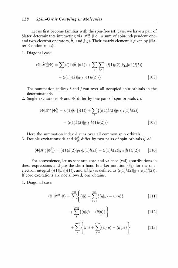
Let us first become familiar with the spin-free (sf) case: we have a pair ofSlater determinants interacting via Hsf

þ (i.e., a sum of spin-independent one-and two-electron operators, h1 and g12). Their matrix element is given by (Sla-ter–Condon rules):

1. Diagonal case:

hjHsfþji ¼

Xi

ið1Þh jh1 ið1Þj i þX

i

Xj> i

f ið1Þjð2Þh jg12 ið1Þjð2Þj i

ið1Þjð2Þh jg12jjð1Þið2Þig ½108

The summation indices i and j run over all occupied spin orbitals in thedeterminant .

2. Single excitations: and ji differ by one pair of spin orbitals i; j.

hjHsfþj

jii ¼ hið1Þjh1j jð1Þi þ

Xk

fhið1Þkð2Þjg12j jð1Þkð2Þi

hið1Þkð2Þjg12jkð1Þjð2Þig ½109

Here the summation index k runs over all common spin orbitals.3. Double excitations: and

jlik differ by two pairs of spin orbitals ij; kl.

hjHsfþj

jliki ¼ hið1Þkð2Þjg12jjð1Þlð2Þi hið1Þkð2Þjg12jlð1Þjð2Þi ½110

For convenience, let us separate core and valence (val) contributions inthese expressions and use the short-hand bra–ket notation hij ji for the one-electron integral hið1Þjh1j jð1Þi, and hikj jli is defined as hið1Þkð2Þjg12j jð1Þlð2Þi.If core excitations are not allowed, one obtains:

1. Diagonal case:

hjHsfþji ¼

Xval

i

hijii þXval

j> i

fhijjiji hijjjiig(

½111

þXcore

j

fhijjiji ijjjiih g)

½112

þXcore

i

hijii þXcore

j>i

fhijjiji hijjjiig( )

½113

128 Spin–Orbit Coupling in Molecules

2. Single excitations: and ji differ by one pair of valence spin orbitals i; j.

hjHsfþj

jii ¼ hij ji þ

Xval

k

fhikjjki hikjkjig ½114

þXcore

k

fhikj jki hikjkjig ½115

3. Double excitations: and jlik differ by two pairs of valence spin orbitals

ij; kl.

hjHsfþj

jliki ¼ hikjjli ikjljih ½116

We see that integrals with core indices contribute solely to the diagonaland the single excitation cases. Because frozen-core orbitals are common to alldeterminants by definition, we may interchange the sums over determinantsand core orbitals. The pure core terms [113] are constant and are convenientlyadded to the nuclear repulsion. After summing over the core indices, the mixedcore–valence integrals, [112] and [115], can be added to the correspondingone-electron integrals hijii and hij ji, respectively. One has to be aware, how-ever, that this summation includes an integration over the spin of the core elec-trons. For a Coulomb integral hikj jki, the same rule applies as for thecorresponding one-electron integral hijji; it survives if the spin of orbitals iand j are equal, whatever the spin of k may be. Because each spatial core orbi-tal is occupied by two electrons, it contributes two Coulomb integrals.Exchange integrals hikjkji, on the other hand, integrate to zero if the spin ofk differs from the spin of i and j. Therefore only one of the exchange integralswill survive. Since the Hamiltonian is spin-independent, the spin part inte-grates to one, irrespective whether it amounts to haajaai or hbbjbbi.

The Frozen-Core Spin–Orbit HamiltonianThe frozen-core (fc) approach is not restricted to spin-independent elec-

tronic interactions; the spin–orbit (SO) interaction between core and valenceelectrons can be expressed by a sum of Coulomb- and exchange-type opera-tors. The matrix element formulas can be derived in a similar way as the Sla-ter–Condon rules.27 Here, it is not important whether the Breit-Pauli spin–orbit operators or their no-pair analogs are employed as these are structurallyequivalent. Differences with respect to the Slater–Condon rules occur due tothe symmetry properties of the angular momentum operators and because ofthe presence of the spin–other-orbit interaction. It is easily shown by partialintegration that the linear momentum operator ~p is antisymmetric with respect

to orbital exchange, and the same applies to~‘ ¼ ~r ~p. Therefore, spin–orbit

Spin–Orbit Hamiltonians 129

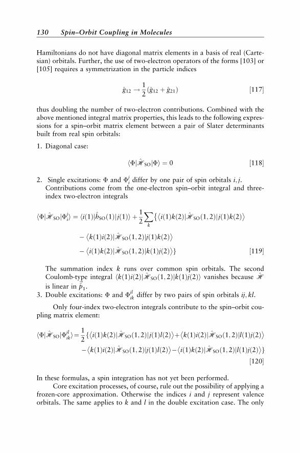
Hamiltonians do not have diagonal matrix elements in a basis of real (Carte-sian) orbitals. Further, the use of two-electron operators of the forms [103] or[105] requires a symmetrization in the particle indices

g12 !1

2ðg12 þ g21Þ ½117

thus doubling the number of two-electron contributions. Combined with theabove mentioned integral matrix properties, this leads to the following expres-sions for a spin–orbit matrix element between a pair of Slater determinantsbuilt from real spin orbitals:

1. Diagonal case:

hjHSOji ¼ 0 ½118

2. Single excitations: and ji differ by one pair of spin orbitals i; j.

Contributions come from the one-electron spin–orbit integral and three-index two-electron integrals

hjHSOjjii ¼ hið1ÞjhSOð1Þj jð1Þi þ

1

2

Xk

ið1Þkð2ÞjHSOð1; 2Þj jð1Þkð2Þ

kð1Þið2ÞjHSOð1;2Þjjð1Þkð2Þ ið1Þkð2ÞjHSOð1;2Þjkð1Þjð2Þ

g ½119

The summation index k runs over common spin orbitals. The secondCoulomb-type integral hkð1Þið2ÞjHSOð1; 2Þjkð1Þjð2Þi vanishes because H

is linear in ~p1.3. Double excitations: and

jlik differ by two pairs of spin orbitals ij; kl.

Only four-index two-electron integrals contribute to the spin–orbit cou-pling matrix element:

hjHSOjjliki¼

1

2f ið1Þkð2ÞjHSOð1; 2Þj jð1Þlð2Þ

þ kð1Þið2ÞjHSOð1; 2Þjlð1Þjð2Þ

kð1Þið2ÞjHSOð1; 2Þjjð1Þlð2Þ

ið1Þkð2ÞjHSOð1; 2Þjlð1Þjð2Þ

g½120

In these formulas, a spin integration has not yet been performed.Core excitation processes, of course, rule out the possibility of applying a

frozen-core approximation. Otherwise the indices i and j represent valenceorbitals. The same applies to k and l in the double excitation case. The only

130 Spin–Orbit Coupling in Molecules

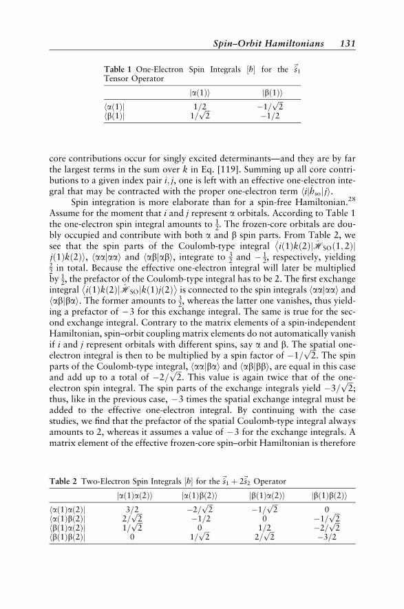
core contributions occur for singly excited determinants—and they are by farthe largest terms in the sum over k in Eq. [119]. Summing up all core contri-butions to a given index pair i; j, one is left with an effective one-electron inte-gral that may be contracted with the proper one-electron term hijhsoj ji.

Spin integration is more elaborate than for a spin-free Hamiltonian.28

Assume for the moment that i and j represent a orbitals. According to Table 1the one-electron spin integral amounts to 1

2. The frozen-core orbitals are dou-bly occupied and contribute with both a and b spin parts. From Table 2, wesee that the spin parts of the Coulomb-type integral ið1Þkð2ÞjHSOð1; 2Þj

jð1Þkð2Þi, haajaai and habjabi, integrate to 3

2 and 12, respectively, yielding

22 in total. Because the effective one-electron integral will later be multipliedby 1

2, the prefactor of the Coulomb-type integral has to be 2. The first exchangeintegral ið1Þkð2ÞjHSOjkð1Þjð2Þ

is connected to the spin integrals haajaai and

habjbai. The former amounts to 32, whereas the latter one vanishes, thus yield-

ing a prefactor of 3 for this exchange integral. The same is true for the sec-ond exchange integral. Contrary to the matrix elements of a spin-independentHamiltonian, spin–orbit coupling matrix elements do not automatically vanishif i and j represent orbitals with different spins, say a and b. The spatial one-electron integral is then to be multiplied by a spin factor of 1=

ffiffiffi2p

. The spinparts of the Coulomb-type integral, haajbai and habjbbi, are equal in this caseand add up to a total of 2=

ffiffiffi2p

. This value is again twice that of the one-electron spin integral. The spin parts of the exchange integrals yield 3=

ffiffiffi2p

;thus, like in the previous case, 3 times the spatial exchange integral must beadded to the effective one-electron integral. By continuing with the casestudies, we find that the prefactor of the spatial Coulomb-type integral alwaysamounts to 2, whereas it assumes a value of 3 for the exchange integrals. Amatrix element of the effective frozen-core spin–orbit Hamiltonian is therefore

Table 1 One-Electron Spin Integrals ½h for the ~s1

Tensor Operator

jað1Þi jbð1Þihað1Þj 1=2 1=

ffiffiffi2p

hbð1Þj 1=ffiffiffi2p

1=2

Table 2 Two-Electron Spin Integrals ½h for the ~s1 þ 2~s2 Operator

jað1Það2Þi jað1Þbð2Þi jbð1Það2Þi jbð1Þbð2Þihað1Það2Þj 3=2 2=

ffiffiffi2p

1=ffiffiffi2p

0hað1Þbð2Þj 2=

ffiffiffi2p

1=2 0 1=ffiffiffi2p

hbð1Það2Þj 1=ffiffiffi2p

0 1=2 2=ffiffiffi2p

hbð1Þbð2Þj 0 1=ffiffiffi2p

2=ffiffiffi2p

3=2

Spin–Orbit Hamiltonians 131

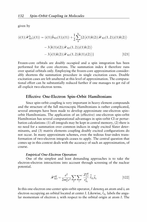
given by

hið1ÞjHfcSOj jð1Þi ¼ hið1ÞjhSOð1Þj jð1Þi þ

1

2

Xfc

k

f2 ið1Þkð2ÞjHSOð1; 2Þj jð1Þkð2Þ

3 kð1Þið2ÞjHSOð1; 2Þj jð1Þkð2Þ

3 ið1Þkð2ÞjHSOð1; 2Þjkð1Þ jð2Þ

g ½121

Frozen-core orbitals are doubly occupied and a spin integration has beenperformed for the core electrons. The summation index k therefore runsover spatial orbitals only. Employing the frozen-core approximation consider-ably shortens the summation procedure in single excitation cases. Doubleexcitation cases are left unaltered at this level of approximation. The computa-tional effort can be substantially reduced further if one manages to get rid ofall explicit two-electron terms.

Effective One-Electron Spin–Orbit Hamiltonians

Since spin–orbit coupling is very important in heavy element compoundsand the structure of the full microscopic Hamiltonians is rather complicated,several attempts have been made to develop approximate one-electron spin–orbit Hamiltonians. The application of an (effective) one-electron spin–orbitHamiltonian has several computational advantages in spin–orbit CI or pertur-bation calculations: (1) all integrals may be kept in central memory, (2) there isno need for a summation over common indices in singly excited Slater deter-minants, and (3) matrix elements coupling doubly excited configurations donot occur. In many approximate schemes, even the tedious four-index trans-formation of two-electron integrals ceases to apply. The central question thatcomes up in this context deals with the accuracy of such an approximation, ofcourse.

Empirical One-Electron OperatorsOne of the simplest and least demanding approaches is to take the

electron–electron interactions into account through screening of the nuclearpotential.

HeffSO ¼

e2

2m2e c2

XI

Xi

0 ZeffI;‘

r3IiI

~‘IiI

~siI ½122

In this one-electron one-center spin–orbit operator, I denotes an atom and iI an

electron occupying an orbital located at center I. Likewise,~‘IiI labels the angu-

lar momentum of electron iI with respect to the orbital origin at atom I. The

132 Spin–Orbit Coupling in Molecules

prime on the second summation (over electrons) indicates that it includes onlythe open shell of an atom I with azimuthal quantum number ‘.

The effective nuclear charge ZeffI;‘ is parameterized to fit experimental

fine-structure splittings of one or more electronic states on atom I. Frequently,this is achieved by estimating a spin–orbit coupling parameter on the basis ofthe Lande interval rule (see the later subsection on this rule). This procedurehas serious drawbacks, however. Open-shell electronic states of heavy atoms,in particular, are often not well separated energetically and may interact viaspin–orbit coupling. In these cases, the multiplet splitting does not followthe Lande pattern, according to which neighboring fine-structure levels oughtto be separated by EðJÞ EðJ 1Þ ¼ ASOJ in first order. Furthermore, in lightatoms spin–spin coupling contributes to the deviation of the atomic splittingfrom the Lande interval rule.

Higher-order spin–orbit effects can be determined by quasi–degenerateperturbation theory (see the section on Computational Aspects). In thisapproach, an interaction matrix is set up including all electrostatic andspin–orbit coupling matrix elements between the states under consideration.Diagonalization of this matrix directly yields the fine-structure splitting. Thereverse procedure may be used for fitting the effective nuclear charge in expres-sion [122]. In principle, the interaction matrix can be diagonalized for variouscoupling strengths, and the spin–orbit parameter is then fitted to reproduce thesplitting in a least-squares sense. However, the deperturbation of an experi-mental spectrum is complicated by the fact that higher-order spin–orbit shiftsdepend both on the location of fictitious spin-free states and the spin–orbitcoupling parameter. If the spin–orbit splitting is small compared to the termenergy separation by Coulombic repulsion, a weighted average of the termenergies may serve as zero-order energies.29 For heavy atoms, the latterapproximation is not applicable; instead excitation energies are determinedfrom correlated ab initio calculations employing a spin-free Hamiltonian.Examples for the latter procedure may be found in Refs. 30–32.

Blume and Watson33 showed in 1962 that only parts of the two-electronspin–orbit interaction may be expressed in the form [122]. According to theseauthors, the neglect of the remaining terms leads to a dependence of the effec-tive nuclear charge from a particular state. For dn configurations, for example,they found that Zeff

I;‘ can vary by as much as 20%.34

Pseudo-Potential Spin–Orbit OperatorsMost common among the approximate spin–orbit Hamiltonians are

those derived from relativistic effective core potentials (RECPs).35–38 Spin–orbit coupling operators for pseudo-potentials were developed in the1970s.39,40 In the meantime, different schools have devised different proce-dures for tailoring such operators. All these procedures to parameterize thespin–orbit interaction for pseudo-potentials have one thing in common: Thepredominant action of the spin–orbit operator has to be transferred from

Spin–Orbit Hamiltonians 133

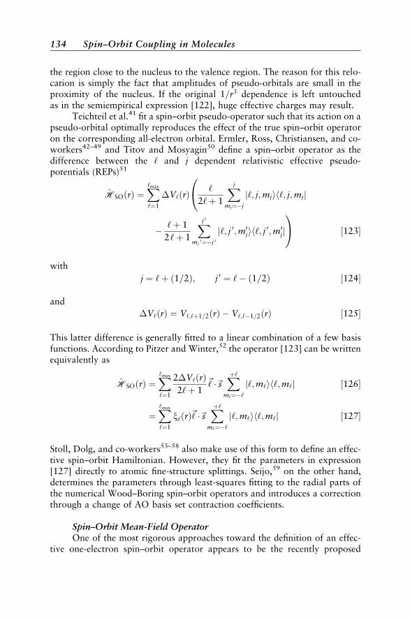
the region close to the nucleus to the valence region. The reason for this relo-cation is simply the fact that amplitudes of pseudo-orbitals are small in theproximity of the nucleus. If the original 1=r3 dependence is left untouchedas in the semiempirical expression [122], huge effective charges may result.

Teichteil et al.41 fit a spin–orbit pseudo-operator such that its action on apseudo-orbital optimally reproduces the effect of the true spin–orbit operatoron the corresponding all-electron orbital. Ermler, Ross, Christiansen, and co-workers42–49 and Titov and Mosyagin50 define a spin–orbit operator as thedifference between the ‘ and j dependent relativistic effective pseudo-potentials (REPs)51

HSOðrÞ ¼X‘max

‘¼1

V‘ðrÞ‘

2‘þ 1

Xj

mj¼j

j‘; j;mjih‘; j;mjj

0@

‘þ 1

2‘þ 1

Xj 0

mj0¼j 0j‘; j 0;m0jih‘; j 0;m0jj

1A ½123

with

j ¼ ‘þ ð1=2Þ; j 0 ¼ ‘ ð1=2Þ ½124

and

V‘ðrÞ ¼ V‘;‘þ1=2ðrÞ V‘;‘1=2ðrÞ ½125

This latter difference is generally fitted to a linear combination of a few basisfunctions. According to Pitzer and Winter,52 the operator [123] can be writtenequivalently as

HSOðrÞ ¼X‘max

‘¼1

2V‘ðrÞ2‘þ 1

~‘ ~sXþ‘

m‘¼‘j‘;m‘ih‘;m‘j ½126

¼X‘max

‘¼1

x‘ðrÞ~‘ ~sXþ‘

m‘¼‘j‘;m‘ih‘;m‘j ½127

Stoll, Dolg, and co-workers53–58 also make use of this form to define an effec-tive spin–orbit Hamiltonian. However, they fit the parameters in expression[127] directly to atomic fine-structure splittings. Seijo,59 on the other hand,determines the parameters through least-squares fitting to the radial parts ofthe numerical Wood–Boring spin–orbit operators and introduces a correctionthrough a change of AO basis set contraction coefficients.

Spin–Orbit Mean-Field OperatorOne of the most rigorous approaches toward the definition of an effec-

tive one-electron spin–orbit operator appears to be the recently proposed

134 Spin–Orbit Coupling in Molecules

spin–orbit mean-field Hamiltonian.60 It constitutes an extension of the frozen-core approximation.

In our effort to get rid of all explicit two-electron terms, we may in mostcases neglect four-index spin–orbit integrals (case 3, Eq. [120]), since theymake a minor contribution to the total spin–orbit coupling matrix elementbetween two CI wave functions. However, unacceptable errors result—in par-ticular for molecules built from light constituents—if also all three-index two-electron valence integrals (case 2, Eq. [119]) are set to zero. A much bettereffective one-electron spin–orbit Hamiltonian is obtained when the frozen-core summation over k in ansatz [121] is extended to the valence space andan average valence orbital occupation—corresponding, for instance, to theHartree–Fock configuration—is assumed. Partially filled orbitals are takeninto account through occupation numbers nk, ranging from 0 to 2. Further,the two-electron spin–orbit interaction of partially filled orbitals k is averagedover a and b spin orientations before spin-integration. A matrix element of thiseffective one-electron spin–orbit mean-field (mf) Hamiltonian is given by

hið1ÞjHmfSOj jð1Þi¼ ið1ÞjhSOð1Þj jð1Þ

D Eþ 1

2

Xk

nkf2 ið1Þkð2ÞjHSOð1; 2Þjjð1Þkð2Þ

3 kð1Þið2ÞjHSOð1; 2Þjjð1Þkð2Þ

3 ið1Þkð2ÞjHSOð1; 2Þjkð1Þjð2Þ

g ½128

The summation index k now runs over all spatial molecular orbitals.The molecular spin–orbit mean-field Hamiltonian appears to approxi-

mate very well the full one- and two-particle operator. For the platinumatom, a deviation from the full operator result of less than 4 cm1 out of a totalof 4000 cm1 was observed (i.e., the error amounts to less than 0:1%).60 Evenlight molecules, where the two-electron contributions to the total matrix ele-ment are in the order of 50%, may be treated in this approximation if the lead-ing configurations of the considered electronic states are singly excited withrespect to each other. The singlet–triplet transition matrix element of etheneand the ground-state splitting of HC6Hþ, NC5Hþ, and NC4Nþ fall into thisclass;61,62 here errors did not exceed 1%.

Like all effective one-electron approaches, the mean-field approximationconsiderably quickens the calculation of spin–orbit coupling matrix elements.Nevertheless, the fact that the construction of the molecular mean-field neces-sitates the evaluation of two-electron spin–orbit integrals in the complete AObasis represents a serious bottleneck in large applications. An enormous speed-up can be achieved if a further approximation is introduced and the molecularmean field is replaced by a sum of atomic mean fields. In this case, only two-electron integrals for basis functions located at the same center have to beevaluated. This idea is based on two observations: first, the spin–orbitHamiltonian exhibits a 1=r3 radial dependence and falls off much faster

Spin–Orbit Hamiltonians 135

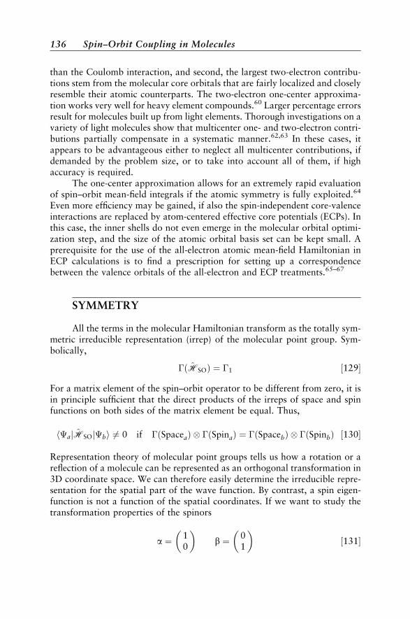
than the Coulomb interaction, and second, the largest two-electron contribu-tions stem from the molecular core orbitals that are fairly localized and closelyresemble their atomic counterparts. The two-electron one-center approxima-tion works very well for heavy element compounds.60 Larger percentage errorsresult for molecules built up from light elements. Thorough investigations on avariety of light molecules show that multicenter one- and two-electron contri-butions partially compensate in a systematic manner.62,63 In these cases, itappears to be advantageous either to neglect all multicenter contributions, ifdemanded by the problem size, or to take into account all of them, if highaccuracy is required.

The one-center approximation allows for an extremely rapid evaluationof spin–orbit mean-field integrals if the atomic symmetry is fully exploited.64

Even more efficiency may be gained, if also the spin-independent core-valenceinteractions are replaced by atom-centered effective core potentials (ECPs). Inthis case, the inner shells do not even emerge in the molecular orbital optimi-zation step, and the size of the atomic orbital basis set can be kept small. Aprerequisite for the use of the all-electron atomic mean-field Hamiltonian inECP calculations is to find a prescription for setting up a correspondencebetween the valence orbitals of the all-electron and ECP treatments.65–67

SYMMETRY

All the terms in the molecular Hamiltonian transform as the totally sym-metric irreducible representation (irrep) of the molecular point group. Sym-bolically,

ðHSOÞ ¼ 1 ½129

For a matrix element of the spin–orbit operator to be different from zero, it isin principle sufficient that the direct products of the irreps of space and spinfunctions on both sides of the matrix element be equal. Thus,

hajHSOjbi 6¼ 0 if ðSpaceaÞ ðSpinaÞ ¼ ðSpacebÞ ðSpinbÞ ½130

Representation theory of molecular point groups tells us how a rotation or areflection of a molecule can be represented as an orthogonal transformation in3D coordinate space. We can therefore easily determine the irreducible repre-sentation for the spatial part of the wave function. By contrast, a spin eigen-function is not a function of the spatial coordinates. If we want to study thetransformation properties of the spinors

a ¼ 10

b ¼ 0

1

½131

136 Spin–Orbit Coupling in Molecules

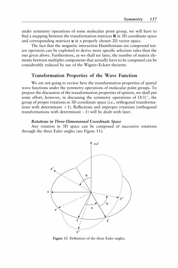
under symmetry operations of some molecular point group, we will have tofind a mapping between the transformation matrices R in 3D coordinate spaceand corresponding matrices u in a properly chosen 2D vector space.

The fact that the magnetic interaction Hamiltonians are compound ten-sor operators can be exploited to derive more specific selection rules than theone given above. Furthermore, as we shall see later, the number of matrix ele-ments between multiplet components that actually have to be computed can beconsiderably reduced by use of the Wigner–Eckart theorem.

Transformation Properties of the Wave Function

We are not going to review here the transformation properties of spatialwave functions under the symmetry operations of molecular point groups. Toprepare the discussion of the transformation properties of spinors, we shall putsome effort, however, in discussing the symmetry operations of O(3)þ, thegroup of proper rotations in 3D coordinate space (i.e., orthogonal transforma-tions with determinant þ1). Reflections and improper rotations (orthogonaltransformations with determinant 1) will be dealt with later.

Rotations in Three-Dimensional Coordinate SpaceAny rotation in 3D space can be composed of successive rotations

through the three Euler angles (see Figure 11):

z,z′

x

y y′

y′′

z′′

x′

x′′

θ

ψφ

Figure 11 Definition of the three Euler angles.

Symmetry 137

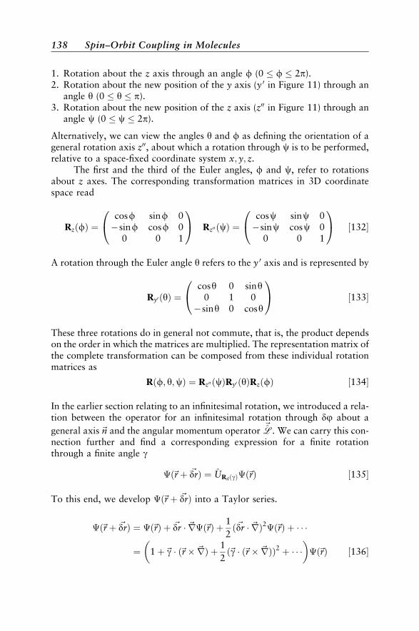
1. Rotation about the z axis through an angle f (0 f 2p).2. Rotation about the new position of the y axis (y 0 in Figure 11) through an

angle y (0 y p).3. Rotation about the new position of the z axis (z00 in Figure 11) through an

angle c (0 c 2p).

Alternatively, we can view the angles y and f as defining the orientation of ageneral rotation axis z00, about which a rotation through c is to be performed,relative to a space-fixed coordinate system x; y; z.

The first and the third of the Euler angles, f and c, refer to rotationsabout z axes. The corresponding transformation matrices in 3D coordinatespace read

RzðfÞ ¼cosf sinf 0sinf cosf 0

0 0 1

0@

1A Rz00 ðcÞ ¼

cosc sinc 0sinc cosc 0

0 0 1

0@

1A ½132

A rotation through the Euler angle y refers to the y 0 axis and is represented by

Ry0 ðyÞ ¼cosy 0 siny

0 1 0siny 0 cosy

0@

1A ½133

These three rotations do in general not commute, that is, the product dependson the order in which the matrices are multiplied. The representation matrix ofthe complete transformation can be composed from these individual rotationmatrices as

Rðf; y;cÞ ¼ Rz00 ðcÞRy0 ðyÞRzðfÞ ½134

In the earlier section relating to an infinitesimal rotation, we introduced a rela-tion between the operator for an infinitesimal rotation through dj about a

general axis~n and the angular momentum operator ~L. We can carry this con-

nection further and find a corresponding expression for a finite rotationthrough a finite angle g

ð~rþ ~drÞ ¼ UR~nðgÞð~rÞ ½135

To this end, we develop ð~rþ ~drÞ into a Taylor series.

ð~rþ ~drÞ ¼ ð~rÞ þ ~dr ~rð~rÞ þ 1

2ð~dr ~rÞ2ð~rÞ þ

¼ 1þ~g ð~r ~rÞ þ 1

2ð~g ð~r ~rÞÞ2 þ

ð~rÞ ½136

138 Spin–Orbit Coupling in Molecules

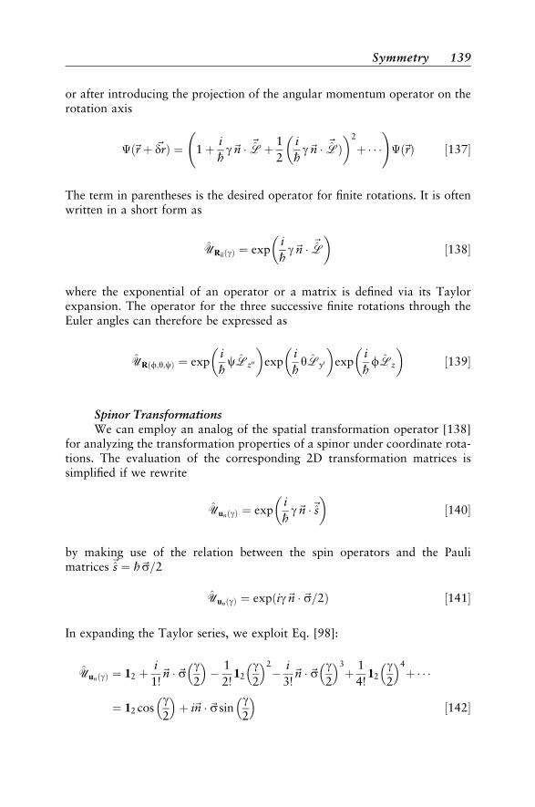
or after introducing the projection of the angular momentum operator on therotation axis

ð~rþ ~drÞ ¼ 1þ i

hg~n ~Lþ 1

2

i

hg~n ~LÞ

2

þ !

ð~rÞ ½137

The term in parentheses is the desired operator for finite rotations. It is oftenwritten in a short form as

UR~nðgÞ ¼ expi

hg~n ~L

½138

where the exponential of an operator or a matrix is defined via its Taylorexpansion. The operator for the three successive finite rotations through theEuler angles can therefore be expressed as

URðf;y;cÞ ¼ expi

hcLz00

exp

i

hyLy0

exp

i

hfLz

½139

Spinor TransformationsWe can employ an analog of the spatial transformation operator [138]

for analyzing the transformation properties of a spinor under coordinate rota-tions. The evaluation of the corresponding 2D transformation matrices issimplified if we rewrite

UunðgÞ ¼ expi

hg~n ~s

½140

by making use of the relation between the spin operators and the Paulimatrices ~s ¼ h~s=2

UunðgÞ ¼ exp ig~n ~s=2ð Þ ½141

In expanding the Taylor series, we exploit Eq. [98]:

UunðgÞ ¼ 12 þi

1!~n ~s g

2

1

2!12

g2

2 i

3!~n ~s g

2

3þ 1

4!12

g2

4þ

¼ 12 cosg2

þ i~n ~ssin

g2

½142

Symmetry 139

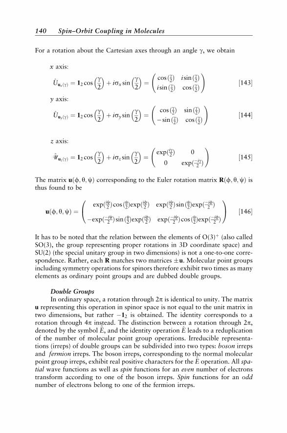
For a rotation about the Cartesian axes through an angle g, we obtain

x axis:

UuxðgÞ ¼ 12 cosg2

þ isx sin

g2

¼

cosðg2Þ isinðg2Þisinðg2Þ cosðg2Þ

!½143

y axis:

UuyðgÞ ¼ 12 cosg2

þ isy sin

g2

¼

cosðg2Þ sinðg2Þsinðg2Þ cosðg2Þ

!½144

z axis:

UuzðgÞ ¼ 12 cosg2

þ isz sin

g2

¼

expðig2Þ 0

0 expðig2 Þ

!½145

The matrix uðf; y;cÞ corresponding to the Euler rotation matrix Rðf; y;cÞ isthus found to be

uðf; y;cÞ ¼expðic2 Þcosðy2Þexpðif2 Þ expðic2 Þsinðy2Þexpðif

2 Þ

expðic2 Þsinðy2Þexpðif2 Þ expðic

2 Þcosðy2Þexpðif2 Þ

0@

1A ½146

It has to be noted that the relation between the elements of O(3)þ (also calledSO(3), the group representing proper rotations in 3D coordinate space) andSU(2) (the special unitary group in two dimensions) is not a one-to-one corre-spondence. Rather, each R matches two matrices u. Molecular point groupsincluding symmetry operations for spinors therefore exhibit two times as manyelements as ordinary point groups and are dubbed double groups.

Double GroupsIn ordinary space, a rotation through 2p is identical to unity. The matrix

u representing this operation in spinor space is not equal to the unit matrix intwo dimensions, but rather 12 is obtained. The identity corresponds to arotation through 4p instead. The distinction between a rotation through 2p,denoted by the symbol E, and the identity operation E leads to a reduplicationof the number of molecular point group operations. Irreducible representa-tions (irreps) of double groups can be subdivided into two types: boson irrepsand fermion irreps. The boson irreps, corresponding to the normal molecularpoint group irreps, exhibit real positive characters for the E operation. All spa-tial wave functions as well as spin functions for an even number of electronstransform according to one of the boson irreps. Spin functions for an oddnumber of electrons belong to one of the fermion irreps.

140 Spin–Orbit Coupling in Molecules

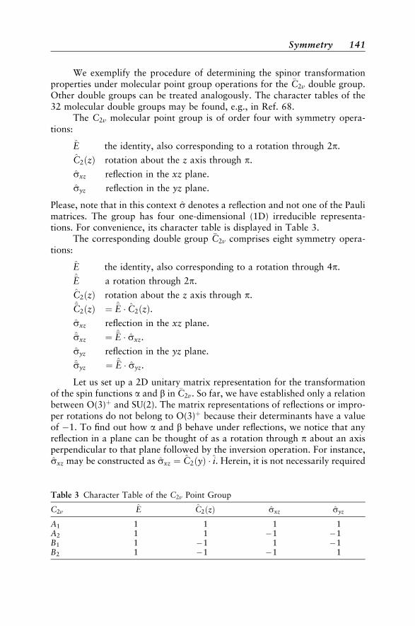
We exemplify the procedure of determining the spinor transformationproperties under molecular point group operations for the C2v double group.Other double groups can be treated analogously. The character tables of the32 molecular double groups may be found, e.g., in Ref. 68.

The C2v molecular point group is of order four with symmetry opera-tions:

E the identity, also corresponding to a rotation through 2p.

C2ðzÞ rotation about the z axis through p.

sxz reflection in the xz plane.

syz reflection in the yz plane.

Please, note that in this context s denotes a reflection and not one of the Paulimatrices. The group has four one-dimensional (1D) irreducible representa-tions. For convenience, its character table is displayed in Table 3.

The corresponding double group C2v comprises eight symmetry opera-tions:

E the identity, also corresponding to a rotation through 4p.E a rotation through 2p.

C2ðzÞ rotation about the z axis through p.C2ðzÞ ¼ E C2ðzÞ.sxz reflection in the xz plane.

sxz ¼ E sxz.

syz reflection in the yz plane.

syz ¼ E syz.

Let us set up a 2D unitary matrix representation for the transformationof the spin functions a and b in C2v. So far, we have established only a relationbetween O(3)þ and SU(2). The matrix representations of reflections or impro-per rotations do not belong to O(3)þ because their determinants have a valueof 1. To find out how a and b behave under reflections, we notice that anyreflection in a plane can be thought of as a rotation through p about an axisperpendicular to that plane followed by the inversion operation. For instance,sxz may be constructed as sxz ¼ C2ðyÞ i. Herein, it is not necessarily required

Table 3 Character Table of the C2v Point Group

C2v E C2ðzÞ sxz syz

A1 1 1 1 1A2 1 1 1 1B1 1 1 1 1B2 1 1 1 1

Symmetry 141

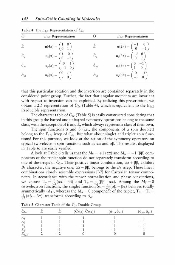
that this particular rotation and the inversion are contained separately in theconsidered point group. Further, the fact that angular momenta are invariantwith respect to inversion can be exploited. By utilizing this prescription, weobtain a 2D representation of C2v (Table 4), which is equivalent to the E1=2

irreducible representation.The character table of C2v (Table 5) is easily constructed considering that

in this group the barred and unbarred symmetry operations belong to the sameclass, with the exception of E and E, which always represent a class of their own.

The spin functions a and b (i.e., the components of a spin doublet)belong to the E1=2 irrep of C2v. But what about singlet and triplet spin func-tions? For this purpose, we look at the action of the symmetry operators ontypical two-electron spin functions such as aa and ab. The results, displayedin Table 6, are easily verified.

A look at Table 6 tells us that the MS ¼ þ1 (aa) and MS ¼ 1 (bb) com-ponents of the triplet spin function do not separately transform according toone of the irreps of C2v. Their positive linear combination, aaþ bb, exhibitsB1 character, the negative one, aa bb, belongs to the B2 irrep. These linearcombinations closely resemble expressions [37] for Cartesian tensor compo-nents. In accordance with the tensor normalization and phase conventions,we choose Ty ¼ iffiffi

2p ðaaþ bbÞ and Tx ¼ 1ffiffi

2p ðbb aaÞ. Among the MS ¼ 0

two-electron functions, the singlet function S0 ¼ 1ffiffi2p ðab baÞ behaves totally

symmetrically (A1), whereas the MS ¼ 0 component of the triplet, T0 ¼ Tz ¼1ffiffi2p ðabþ baÞ, transforms according to A2.

Table 4 The E1=2 Representation of C2v

O E1=2 Representation O E1=2 Representation

E uð4pÞ ¼ 1 00 1

E uð2pÞ ¼ 1 0

0 1

C2 uzðpÞ ¼

i 00 i

C2 uzð3pÞ ¼

i 00 i

sxz uyðpÞ ¼

0 11 0

sxz uyð3pÞ ¼

0 11 0

syz uxðpÞ ¼

0 ii 0

syz uxð3pÞ ¼

0 ii 0

Table 5 Character Table of the C2v Double Group

C2v E E ðC2ðzÞ; C2ðzÞÞ ðsxz; sxzÞ ðsyz; syzÞA1 1 1 1 1 1A2 1 1 1 1 1B1 1 1 1 1 1B2 1 1 1 1 1E1=2 2 2 0 0 0

142 Spin–Orbit Coupling in Molecules

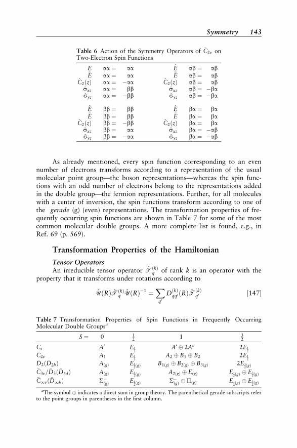
As already mentioned, every spin function corresponding to an evennumber of electrons transforms according to a representation of the usualmolecular point group—the boson representations—whereas the spin func-tions with an odd number of electrons belong to the representations addedin the double group—the fermion representations. Further, for all moleculeswith a center of inversion, the spin functions transform according to one ofthe gerade (g) (even) representations. The transformation properties of fre-quently occurring spin functions are shown in Table 7 for some of the mostcommon molecular double groups. A more complete list is found, e.g., inRef. 69 (p. 569).

Transformation Properties of the Hamiltonian

Tensor OperatorsAn irreducible tensor operator TðkÞ

q of rank k is an operator with theproperty that it transforms under rotations according to

UðRÞTðkÞq UðRÞ1 ¼

Xq0

DðkÞqq0 ðRÞT

ðkÞq0 ½147

Table 6 Action of the Symmetry Operators of C2v onTwo-Electron Spin Functions

E aa ¼ aa E ab ¼ abE aa ¼ aa E ab ¼ ab

C2ðzÞ aa ¼ aa C2ðzÞ ab ¼ absxz aa ¼ bb sxz ab ¼ basyz aa ¼ bb syz ab ¼ ba

E bb ¼ bb E ba ¼ baE bb ¼ bb E ba ¼ ba

C2ðzÞ bb ¼ bb C2ðzÞ ba ¼ basxz bb ¼ aa sxz ba ¼ absyz bb ¼ aa syz ba ¼ ab

Table 7 Transformation Properties of Spin Functions in Frequently OccurringMolecular Double Groupsa

S ¼ 0 12 1 3

2

Cs A0 E12

A0 2A00 2E12

C2v A1 E12

A2 B1 B2 2E12

D2ð D2hÞ AðgÞ E12ðgÞ B1ðgÞ B2ðgÞ B3ðgÞ 2E1

2ðgÞC3v= D3ð D3dÞ AðgÞ E1

2ðgÞ A2ðgÞ EðgÞ E12ðgÞ E3

2ðgÞC1vð D1hÞ þðgÞ E1

2ðgÞ ðgÞ ðgÞ E12ðgÞ E3

2ðgÞ

aThe symbol indicates a direct sum in group theory. The parenthetical gerade subscripts referto the point groups in parentheses in the first column.

Symmetry 143

that is, the components of TðkÞ are transformed among themselves upon acoordinate rotation. The coefficients D

ðkÞqq0 ðRÞ are elements of a 2kþ 1 dimen-

sional irreducible matrix representation DðkÞ of the full rotation group in threedimensions, Oþð3Þ or SOð3Þ. Equivalently, it can be stated that the 2kþ 1components TðkÞ

q with q ranging from k to k form a basis for the irreduci-ble representation DðkÞ of Oþð3Þ. Actually, the coefficients D

ðkÞqq0 ðRÞ are the

same as those obtained from a rotation operation transferring the sphericalharmonic Ykqðy;fÞ (see Eq. [25]) to Ykq0 ðy;fÞ.

The simplest example is a scalar operator Tð0Þ0 with the transformation

property

UðRÞTð0Þ0 UðRÞ1 ¼ T

ð0Þ0 ½148

This means that scalar operators are invariant with respect to rotations incoordinate or spin space. An example for a scalar operator is the Hamiltonian,i.e., the operator of the energy.

A first-rank tensor operator Tð1Þ is also called a vector operator. It hasthree components, T

ð1Þ0 and T

ð1Þ1. Operators of this type are the angular

momentum operators, for instance. Relations between spherical and Cartesiancomponents of first-rank tensor operators are given in Eqs. [36] and [37].

Operating with the components of an arbitrary vector operator Pð1Þ onan eigenfunction juMP

P i of the corresponding operators ðPð1ÞÞ2 and Pð1Þ0 yields

the following results:

Pð1Þ0 ju

MP

P i ¼ hMPjuMP

P i ½149

Pð1Þ1ju

MP

P i ¼ hffiffiffiffiffiffiffiffiffiffiffiffiffiffiffiffiffiffiffiffiffiffiffiffiffiffiffiffiffiffiffiffiffiffiffiffiffiffiffiffiffiffiffiffiffiffiffiffiffiffiffiffiffiffiffiffi12 ½PðPþ 1Þ ðMP 1ÞMP

qjuMP1

P i ½150

Pð1Þ0 conserves the projection MP of P on the z axis, P

ð1Þþ1 increases MP by one

unit, and Pð1Þ1 decreases MP by one unit. The prefactors in Eq. [150] differ

slightly from those obtained in Eq. [74] by operating with step operators onjuM

J i (see the earlier section on step/shift/ladder and tensor operators).A general Cartesian second-rank tensor operator is represented by a

3 3 matrix.

T ð2Þðx; y; zÞ ¼Tð2Þ

xx Tð2Þxy Tð2Þ

xz

Tð2Þyx Tð2Þ

yy Tð2Þyz

Tð2Þzx Tð2Þ

zy Tð2Þzz

0BB@

1CCA ½151

If the Cartesian representation corresponds to an irreducible second-ranktensor, its nine entries are not independent: The four conditions T

ð2Þij ¼ T

ð2Þji

andP

i Tð2Þii ¼ 0 with i; j 2 fx; y; zg reduce the number of independent

144 Spin–Orbit Coupling in Molecules

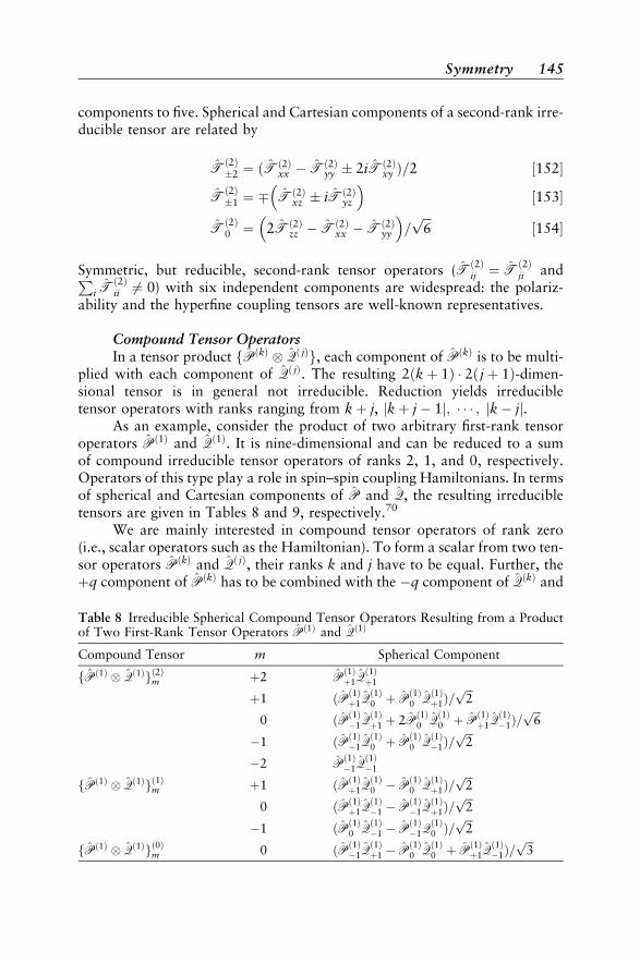
components to five. Spherical and Cartesian components of a second-rank irre-ducible tensor are related by

Tð2Þ2 ¼ ðT

ð2Þxx Tð2Þ

yy 2iTð2Þxy Þ=2 ½152

Tð2Þ1 ¼ Tð2Þ

xz iTð2Þyz

½153

Tð2Þ0 ¼ 2Tð2Þ

zz Tð2Þxx Tð2Þ

yy

=ffiffiffi6p

½154

Symmetric, but reducible, second-rank tensor operators (Tð2Þij ¼ T

ð2Þji andP

i Tð2Þii 6¼ 0) with six independent components are widespread: the polariz-

ability and the hyperfine coupling tensors are well-known representatives.

Compound Tensor OperatorsIn a tensor product fPðkÞ Qð jÞg, each component of PðkÞ is to be multi-

plied with each component of Qð jÞ. The resulting 2ðkþ 1Þ 2ð jþ 1Þ-dimen-sional tensor is in general not irreducible. Reduction yields irreducibletensor operators with ranks ranging from kþ j, jkþ j 1j; ; jk jj.

As an example, consider the product of two arbitrary first-rank tensoroperators Pð1Þ and Qð1Þ. It is nine-dimensional and can be reduced to a sumof compound irreducible tensor operators of ranks 2, 1, and 0, respectively.Operators of this type play a role in spin–spin coupling Hamiltonians. In termsof spherical and Cartesian components of P and Q, the resulting irreducibletensors are given in Tables 8 and 9, respectively.70

We are mainly interested in compound tensor operators of rank zero(i.e., scalar operators such as the Hamiltonian). To form a scalar from two ten-sor operators PðkÞ and Qð jÞ, their ranks k and j have to be equal. Further, theþq component of PðkÞ has to be combined with the q component of QðkÞ and

Table 8 Irreducible Spherical Compound Tensor Operators Resulting from a Productof Two First-Rank Tensor Operators Pð1Þ and Qð1Þ

Compound Tensor m Spherical Component

fPð1Þ Qð1Þgð2Þm þ2 Pð1Þþ1Q

ð1Þþ1

þ1 ðPð1Þþ1Qð1Þ0 þ P

ð1Þ0 Q

ð1Þþ1Þ=

ffiffiffi2p

0 ðPð1Þ1Qð1Þþ1 þ 2P

ð1Þ0 Q

ð1Þ0 þ P

ð1Þþ1Q

ð1Þ1Þ=

ffiffiffi6p

1 ðPð1Þ1Qð1Þ0 þ P

ð1Þ0 Q

ð1Þ1Þ=

ffiffiffi2p

2 Pð1Þ1Q

ð1Þ1

fPð1Þ Qð1Þgð1Þm þ1 ðPð1Þþ1Qð1Þ0 P

ð1Þ0 Q

ð1Þþ1Þ=

ffiffiffi2p

0 ðPð1Þþ1Qð1Þ1 P

ð1Þ1Q

ð1Þþ1Þ=

ffiffiffi2p

1 ðPð1Þ0 Qð1Þ1 P

ð1Þ1Q

ð1Þ0 Þ=

ffiffiffi2p

fPð1Þ Qð1Þgð0Þm 0 ðPð1Þ1Qð1Þþ1 P

ð1Þ0 Q

ð1Þ0 þ P

ð1Þþ1Q

ð1Þ1Þ=

ffiffiffi3p

Symmetry 145

vice versa. Two notations are found in the literature for these tensor productsdiffering only in normalization constants and phase factors. The properly nor-malized product of two tensor operators forming a scalar operator reads71

fPðkÞ QðkÞgð0Þ0 ¼ ð2kþ 1Þ1=2Xþk

q¼k

ð1ÞkqPðkÞq QðkÞq ½155

Instead, we utilize the simplified expression that differs from Eq. [155] by afactor of

ffiffiffiffiffiffiffiffiffiffiffiffiffiffi2kþ 1p

:

ðPðkÞ QðkÞÞ ¼Xþk

q¼1

ð1ÞkqPðkÞq QðkÞq ½156

Tensor Properties of Magnetic Interaction TermsThe operators HSO and HSS are compound tensor operators of rank

zero (scalars) composed of vector (first-rank tensor) operators and matrix (sec-ond-rank tensor) operators. We will make use of this tensorial structure whenit comes to selection rules for the magnetic interaction Hamiltonians andsymmetry relations between their matrix elements. Similar considerationsapply to the molecular rotation Hrot and hyperfine splitting interactionHamiltonians Hhfs.

Spin–Orbit Coupling For the derivation of selection rules, it is sufficientto employ a simplified Hamiltonian. To this end, we rewrite each term in themicroscopic spin–orbit Hamiltonians in form of a scalar product between an

appropriately chosen spatial angular momentum ~L and a spin angular

momentum~S

HSO ¼ ASOðrÞ ~L ~S ½157

Table 9 Irreducible Cartesian Compound Tensor Operators Resulting from a Productof Two First-Rank Tensor Operators Pð1Þ and Qð1Þ

Compound Tensor m Cartesian Component

fPð1Þ Qð1Þgð2Þm þ2 ðPð1Þx Qð1Þx Pð1Þy Qð1Þy þ iPð1Þx Qð1Þy þ iPð1Þy Qð1Þx Þ=2

þ1 ðPð1Þx Qð1Þz þ Pð1Þz Qð1Þx þ iPð1Þy Qð1Þz þ iPð1Þz Qð1Þy Þ=2

0 ð2Pð1Þz Qð1Þz Pð1Þx Qð1Þx Pð1Þy Qð1Þy Þ=ffiffiffi6p

1 ðPð1Þx Qð1Þz þ Pð1Þz Qð1Þx iPð1Þy Qð1Þz iPð1Þz Qð1Þy Þ=2

2 ðPð1Þx Qð1Þx Pð1Þy Qð1Þy iPð1Þx Qð1Þy iPð1Þy Qð1Þx Þ=2

fPð1Þ Qð1Þgð1Þm þ1 ðPð1Þx Qð1Þz Pð1Þz Qð1Þx þ iPð1Þy Qð1Þz iPð1Þz Qð1Þy Þ=2

0 iðPð1Þx Qð1Þy Pð1Þy Qð1Þx Þ=ffiffiffi2p

1 ðPð1Þz Qð1Þx Pð1Þx Qð1Þz iPð1Þz Qð1Þy þ iPð1Þy Qð1Þz Þ=2

fPð1Þ Qð1Þgð0Þm 0 ðPð1Þx Qð1Þx þ Pð1Þy Qð1Þy þ Pð1Þz Qð1Þz Þ=ffiffiffi3p

146 Spin–Orbit Coupling in Molecules

The operator [157] is a phenomenological spin–orbit operator. In addition tobeing useful for symmetry considerations, Eq. [157] can be utilized for settingup a connection between theoretically and experimentally determined fine-structure splittings via the so-called spin–orbit parameter ASO (see the latersection on first-order spin–orbit splitting). In terms of its tensor components,the phenomenological spin–orbit Hamiltonian reads

HSO ¼ ASOðrÞ ~L ~S ½158

¼ ASOðrÞðL0S0 Lþ1S1 L1Sþ1Þ ½159

¼ ASOðrÞðLxSx þ LySy þ LzSzÞ ½160

The phenomenological spin–orbit Hamiltonian ought not to be used forcomputing spin–orbit matrix elements, though. An example for a failure ofsuch a procedure will be discussed in detail in the later subsection on a wordof caution.

Spin–Spin Coupling Although we focus on spin–orbit coupling (SOC),we need to consider the tensorial structure of electronic spin–spin coupling:Second-order SOC mimics perfectly first-order spin–spin coupling and viceversa, so that they cannot be told apart (see the later section on second-orderspin–orbit splitting).

The dipolar spin–spin coupling operators are scalar operators of the formPð1Þ Tð2Þ Qð1Þ. The tensorial structure of HSS becomes apparent if we writethe Breit–Pauli spin–spin coupling operator as

HBPSS ¼

e2h2

2m2e c2

Xi6¼j

8p3dð~rijÞ~si

~sj þ~si~sj

r3ij

~sið3~rij ~rijÞð2Þ~sjÞ

r5ij

( )½161

¼ e2h2

2m2e c2

Xi6¼j

8p3dð~rijÞ~si

~sj þ ~siDð2Þij~sj

)½162

The first term is a tensor of rank zero involving only spin variables. It does notcontribute to the multiplet splitting of an electronic state but yields only a(small) overall shift of the energy and is, henceforth, neglected. The operatorDð2Þij is a traceless (irreducible) second-rank tensor operator, the form of which

in Cartesian components is

Dð2Þij ¼

1

r5ij

r2ij 3x2

ij 3xijyij 3xijzij

3xijyij r2ij 3y2

ij 3yijzij

3xijzij 3yijzij r2ij 3z2

ij

0BB@

1CCA ½163

Symmetry 147

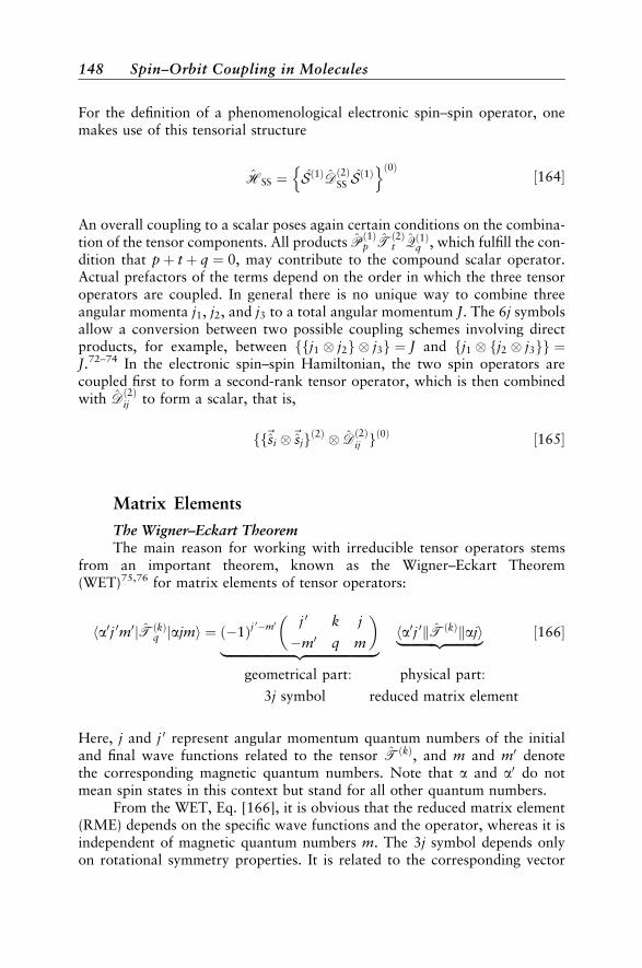
For the definition of a phenomenological electronic spin–spin operator, onemakes use of this tensorial structure

HSS ¼ Sð1ÞDð2ÞSS Sð1Þ

n oð0Þ½164

An overall coupling to a scalar poses again certain conditions on the combina-tion of the tensor components. All products P

ð1Þp T

ð2Þt Qð1Þq , which fulfill the con-

dition that pþ t þ q ¼ 0, may contribute to the compound scalar operator.Actual prefactors of the terms depend on the order in which the three tensoroperators are coupled. In general there is no unique way to combine threeangular momenta j1, j2, and j3 to a total angular momentum J. The 6j symbolsallow a conversion between two possible coupling schemes involving directproducts, for example, between ffj1 j2g j3g ¼ J and fj1 fj2 j3gg ¼J.72–74 In the electronic spin–spin Hamiltonian, the two spin operators arecoupled first to form a second-rank tensor operator, which is then combinedwith D

ð2Þij to form a scalar, that is,

ff~si ~sjgð2Þ Dð2Þij g

ð0Þ ½165

Matrix Elements

The Wigner–Eckart TheoremThe main reason for working with irreducible tensor operators stems

from an important theorem, known as the Wigner–Eckart Theorem(WET)75,76 for matrix elements of tensor operators:

ha0j 0m0jTðkÞq jajmi ¼ ð1Þj

0m0 j 0 k j

m0 q m

|fflfflfflfflfflfflfflfflfflfflfflfflfflfflfflfflfflfflfflfflfflfflzfflfflfflfflfflfflfflfflfflfflfflfflfflfflfflfflfflfflfflfflfflffl ha0j 0kTðkÞkaji|fflfflfflfflfflfflfflfflfflfflfflzfflfflfflfflfflfflfflfflfflfflffl ½166

geometrical part: physical part:

3j symbol reduced matrix element

Here, j and j 0 represent angular momentum quantum numbers of the initialand final wave functions related to the tensor TðkÞ, and m and m0 denotethe corresponding magnetic quantum numbers. Note that a and a0 do notmean spin states in this context but stand for all other quantum numbers.

From the WET, Eq. [166], it is obvious that the reduced matrix element(RME) depends on the specific wave functions and the operator, whereas it isindependent of magnetic quantum numbers m. The 3j symbol depends onlyon rotational symmetry properties. It is related to the corresponding vector

148 Spin–Orbit Coupling in Molecules

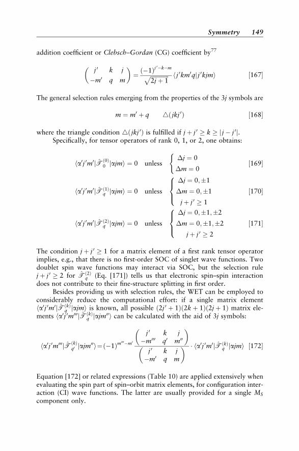
addition coefficient or Clebsch–Gordan (CG) coefficient by77

j 0 k j

m0 q m

¼ ð1Þj

0kmffiffiffiffiffiffiffiffiffiffiffiffiffi2jþ 1

p h j 0km0qj j 0kjmi ½167

The general selection rules emerging from the properties of the 3j symbols are

m ¼ m0 þ q 4ð jkj 0Þ ½168

where the triangle condition 4ð jkj 0Þ is fulfilled if jþ j 0 k j j j 0j.Specifically, for tensor operators of rank 0, 1, or 2, one obtains:

ha0j 0m0jTð0Þ0 jajmi ¼ 0 unless

j ¼ 0

m ¼ 0

(½169

ha0j 0m0jTð1Þq jajmi ¼ 0 unless

j ¼ 0;1

m ¼ 0;1

jþ j 0 1

8><>: ½170

ha0j 0m0jTð2Þq jajmi ¼ 0 unless

j ¼ 0;1;2

m ¼ 0;1;2

jþ j 0 2

8><>: ½171

The condition jþ j 0 1 for a matrix element of a first rank tensor operatorimplies, e.g., that there is no first-order SOC of singlet wave functions. Twodoublet spin wave functions may interact via SOC, but the selection rulejþ j 0 2 for Tð2Þ

q (Eq. [171]) tells us that electronic spin–spin interactiondoes not contribute to their fine-structure splitting in first order.

Besides providing us with selection rules, the WET can be employed toconsiderably reduce the computational effort: if a single matrix elementha0j 0m0jTðkÞ

q jajmi is known, all possible ð2j 0 þ 1Þð2kþ 1Þð2jþ 1Þ matrix ele-ments ha0j 0m000jTðkÞ

q jajm00i can be calculated with the aid of 3j symbols:

ha0j 0m000jTðkÞq0 jajm00i¼ð1Þm

000m0

j 0 k jm000 q0 m00

j 0 k jm0 q m

ha0j 0m0jTðkÞq jajmi ½172

Equation [172] or related expressions (Table 10) are applied extensively whenevaluating the spin part of spin–orbit matrix elements, for configuration inter-action (CI) wave functions. The latter are usually provided for a single MS

component only.

Symmetry 149

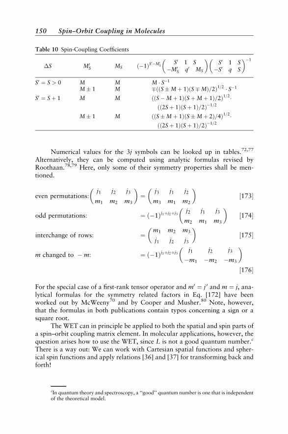
Numerical values for the 3j symbols can be looked up in tables.72,77

Alternatively, they can be computed using analytic formulas revised byRoothaan.78,79 Here, only some of their symmetry properties shall be men-tioned.

even permutations:j1 j2 j3

m1 m2 m3

¼

j3 j1 j2

m3 m1 m2

½173

odd permutations: ¼ ð1Þj1þj2þj3j2 j1 j3

m2 m1 m3

½174

interchange of rows: ¼m1 m2 m3

j1 j2 j3

½175

m changed to m: ¼ ð1Þj1þj2þj3j1 j2 j3

m1 m2 m3

½176

For the special case of a first-rank tensor operator and m0 ¼ j 0 and m ¼ j, ana-lytical formulas for the symmetry related factors in Eq. [172] have beenworked out by McWeeny70 and by Cooper and Musher.80 Note, however,that the formulas in both publications contain typos concerning a sign or asquare root.

The WET can in principle be applied to both the spatial and spin parts ofa spin–orbit coupling matrix element. In molecular applications, however, thequestion arises how to use the WET, since L is not a good quantum number.c

There is a way out: We can work with Cartesian spatial functions and spher-ical spin functions and apply relations [36] and [37] for transforming back andforth!

Table 10 Spin-Coupling Coefficients

S M0S MS ð1ÞS

0M0S

S0 1 SM0

S q0 MS

S0 1 SS0 q S

1

S0 ¼ S > 0 M M M S1

M 1 M ððSMþ 1ÞðSMÞ=2Þ1=2 S1

S0 ¼ Sþ 1 M M ððSMþ 1ÞðSþMþ 1Þ=2Þ1=2ðð2Sþ 1ÞðSþ 1Þ=2Þ1=2

M 1 M ððSMþ 1ÞðSMþ 2Þ=4Þ1=2ðð2Sþ 1ÞðSþ 1Þ=2Þ1=2

cIn quantum theory and spectroscopy, a ‘‘good’’ quantum number is one that is independentof the theoretical model.

150 Spin–Orbit Coupling in Molecules

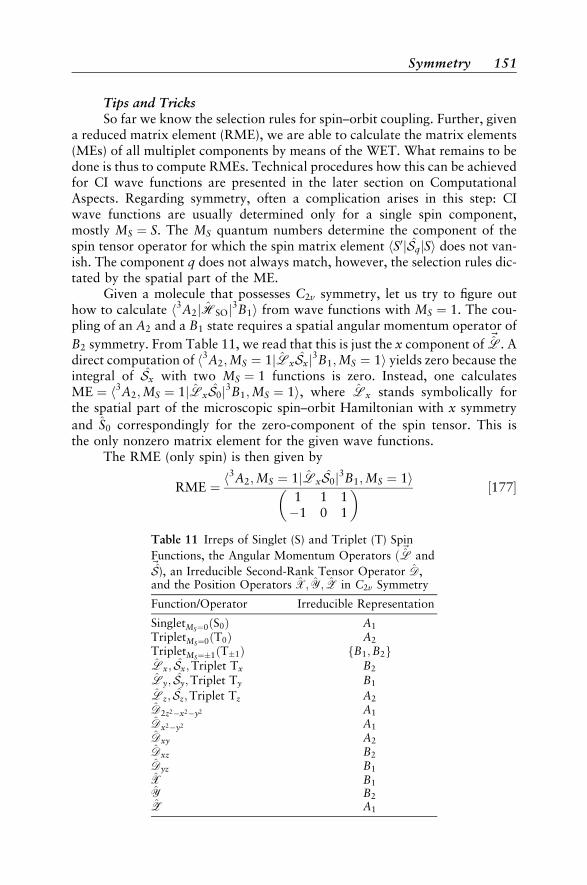
Tips and TricksSo far we know the selection rules for spin–orbit coupling. Further, given

a reduced matrix element (RME), we are able to calculate the matrix elements(MEs) of all multiplet components by means of the WET. What remains to bedone is thus to compute RMEs. Technical procedures how this can be achievedfor CI wave functions are presented in the later section on ComputationalAspects. Regarding symmetry, often a complication arises in this step: CIwave functions are usually determined only for a single spin component,mostly MS ¼ S. The MS quantum numbers determine the component of thespin tensor operator for which the spin matrix element hS0jSqjSi does not van-ish. The component q does not always match, however, the selection rules dic-tated by the spatial part of the ME.

Given a molecule that possesses C2v symmetry, let us try to figure outhow to calculate h3A2jHSOj3B1i from wave functions with MS ¼ 1. The cou-pling of an A2 and a B1 state requires a spatial angular momentum operator of

B2 symmetry. From Table 11, we read that this is just the x component of ~L. A

direct computation of h3A2;MS ¼ 1jLxSxj3B1;MS ¼ 1i yields zero because theintegral of Sx with two MS ¼ 1 functions is zero. Instead, one calculatesME ¼ h3A2;MS ¼ 1jLxS0j3B1;MS ¼ 1i, where Lx stands symbolically forthe spatial part of the microscopic spin–orbit Hamiltonian with x symmetry

and S0 correspondingly for the zero-component of the spin tensor. This isthe only nonzero matrix element for the given wave functions.

The RME (only spin) is then given by

RME ¼ h3A2;MS ¼ 1jLxS0j3B1;MS ¼ 1i

1 1 11 0 1

½177

Table 11 Irreps of Singlet (S) and Triplet (T) Spin

Functions, the Angular Momentum Operators ð ~L and~S), an Irreducible Second-Rank Tensor Operator D,and the Position Operators X; Y; Z in C2v Symmetry

Function/Operator Irreducible Representation

SingletMS¼0ðS0Þ A1

TripletMS¼0ðT0Þ A2

TripletMS¼1ðT1Þ fB1;B2gLx; Sx;Triplet Tx B2

Ly; Sy;Triplet Ty B1

Lz; Sz;Triplet Tz A2

D2z2x2y2 A1

Dx2y2 A1

Dxy A2

Dxz B2

Dyz B1

X B1

Y B2

Z A1

Symmetry 151

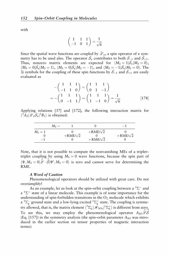
with

1 1 11 0 1

¼ 1ffiffiffi

6p

Since the spatial wave functions are coupled by Lx, a spin operator of x sym-metry has to be used also. The operator Sx contributes to both S1 and Sþ1.Thus, nonzero matrix elements are expected for hMS ¼ 1jSxjMS ¼ 0i,hMS ¼ 0jSxjMS ¼ 1i, hMS ¼ 0jSxjMS ¼ 1i, and hMS ¼ 1jSxjMS ¼ 0i. The3j symbols for the coupling of these spin functions by S1 and Sþ1 are easilyevaluated as

1 1 1

1 1 0

¼

1 1 1

0 1 1

¼ 1 1 1

0 1 1

¼

1 1 1

1 1 0

¼ 1ffiffiffi

6p ½178

Applying relations [37] and [172], the following interaction matrix forh3A2jLxSxj3B1i is obtained:

MS ¼ 1 0 1

MS ¼ 1 0 þRME/ffiffiffi2p

00 þRME/

ffiffiffi2p

0 þRME/ffiffiffi2p

1 0 þRME/ffiffiffi2p

0

Note, that it is not possible to compute the nonvanishing MEs of a triplet–triplet coupling by using MS ¼ 0 wave functions, because the spin part of

h;MS ¼ 0j ~L ~Sj0;MS ¼ 0i is zero and cannot serve for determining theRME.

A Word of CautionPhenomenological operators should be utilized with great care. Do not

oversimplify!As an example, let us look at the spin–orbit coupling between a 3 and

a 1þ state of a linear molecule. This example is of some importance for theunderstanding of spin-forbidden transitions in the O2 molecule which exhibitsa 3g ground state and a low-lying excited 1þg state. The coupling is symme-

try allowed, that is, the matrix element h30 jHSOzj1þ0 i is different from zero.

To see this, we may employ the phenomenological operator ASO~L~S

(Eq. [157]) in the symmetry analysis (the spin–orbit parameter ASO was intro-duced in the earlier section on tensor properties of magnetic interactionterms):

152 Spin–Orbit Coupling in Molecules

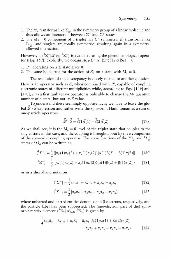
1. The Lz transforms like ðgÞ in the symmetry group of a linear molecule andthus allows an interaction between and þ states.

2. The MS ¼ 0 component of a triplet has symmetry, Sz transforms likeðgÞ, and singlets are totally symmetric, resulting again in a symmetry-allowed interaction.

However, if h30 jHSOzj1þ0 i is evaluated using the phenomenological opera-tor ([Eq. 157]) explicitly, we obtain ASOhjLzjþihT0jSzjS0i ¼ 0:

1. Lz operating on a state gives 0.2. The same holds true for the action of S0 on a state with MS ¼ 0.

The resolution of this discrepancy is closely related to another question:

How is an operator such as~S, when combined with ~

L, capable of couplingelectronic states of different multiplicities while, according to Eqs. [149] and

[150],~S as a first rank tensor operator is only able to change the MS quantum

number of a state, but not its S value.To understand these seemingly opposite facts, we have to leave the glo-

bal ~L ~S expression and rather write the spin–orbit Hamiltonian as a sum of

one-particle operators

~L ~S ¼ ~

‘ð1Þ~sð1Þ þ~‘ð2Þ~sð2Þ ½179

As we shall see, it is the MS ¼ 0 level of the triplet state that couples to thesinglet state in this case, and the coupling is brought about by the z componentof the spin–orbit coupling operator. The wave functions of the 3g and 1þgstates of O2 can be written as

h1þj ¼ 1

2h½pxð1Þpxð2Þ þ pyð1Þpyð2ÞÞðað1Þbð2Þ bð1Það2Þj ½180

j3i ¼ 1

2j½pxð1Þpyð2Þ pyð1Þpxð2ÞÞ að1Þbð2Þ þ bð1Það2Þið ½181

or in a short-hand notation

h1þj ¼ 1

2hpxpx pxpx þ pypy pypyj ½182

j3i ¼ 1

2pxpy þ pxpy pypx pypxi// ½183

where unbarred and barred entities denote a and b electrons, respectively, andthe particle label has been suppressed. The (one-electron part of the) spin–orbit matrix element h30 jHSOzj1þ0 i is given by

1

4hpxpx pxpx þ pypy pypyj½‘0ð1Þs0ð1Þ þ ‘0ð2Þs0ð2Þ

jpxpy þ pxpy pypx pypxi ½184

Symmetry 153

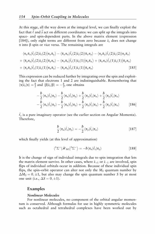
At this stage, all the way down at the integral level, we can finally exploit the

fact that~‘ and ~s act on different coordinates: we can split up the integrals into

space- and spin-dependent parts. In the above matrix element (expression[184]), only eight terms are different from zero because sz does not changea into b spin or vice versa. The remaining integrals are

hpxpxj‘zð2Þszð2Þ pxpy

// pxpxh j‘zð2Þszð2Þjpxpyi hpypyj‘zð2Þszð2Þjpypxi

þ hpypyj‘zð2Þszð2Þ pypxi hpxpx

// //‘zð1Þszð1Þ pypx

// þ pxpxh j‘zð1Þszð1Þ pypxi

//þ hpypyj‘zð1Þszð1Þ pxpyi hpypy

// //‘zð1Þszð1Þ pxpyi// ½185

This expression can be reduced further by integrating over the spin and exploit-ing the fact that electrons 1 and 2 are indistinguishable. Remembering thathajszjai ¼ h

2 and hbjszjbi ¼ h2, one obtains

h

2hpxj‘zjpyi

h

2hpxj‘zjpyi þ

h

2hpyj‘zjpxi þ

h

2hpyj‘zjpxi

h

2hpxj‘zjpyi

h

2pxh j‘zjpyi þ

h

2hpyj‘zjpxi þ

h

2hpyj‘z pxij ½186

‘z is a pure imaginary operator (see the earlier section on Angular Momenta).Therefore,

h

2hpxj‘zjpyi ¼

h

2hpyj‘zjpxi ½187

which finally yields (at this level of approximation)

h1þjHSO3//

¼ hhpxj‘zjpyi ½188

It is the change of sign of individual integrals due to spin integration that letsthe matrix element survive. In other cases, where sþ1 or s1 are involved, spinflips of individual orbitals occur in addition. Because of these individual spinflips, the spin–orbit operator can alter not only the MS quantum number byMS ¼ 0;1, but also may change the spin quantum number S by at mostone unit (i.e., S ¼ 0;1).

Examples

Nonlinear MoleculesFor nonlinear molecules, no component of the orbital angular momen-

tum is conserved. Although formulas for use in highly symmetric moleculessuch as octahedral and tetrahedral complexes have been worked out by

154 Spin–Orbit Coupling in Molecules

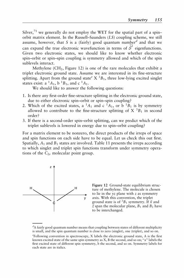
Silver,71 we generally do not employ the WET for the spatial part of a spin–orbit matrix element. In the Russell–Saunders (LS) coupling scheme, we stillassume, however, that S is a (fairly) good quantum numberd and that we

can expand the true electronic wavefunction in terms of~S2

eigenfunctions.Given two electronic states, we should like to know whether electronicspin–orbit or spin–spin coupling is symmetry allowed and which of the spinsublevels interact.

Methylene (CH2, Figure 12) is one of the rare molecules that exhibit atriplet electronic ground state. Assume we are interested in its fine-structuresplitting. Apart from the ground statee X 3B1, three low-lying excited singletstates exist: a 1A1, b 1B1, and c 1A1.

We should like to answer the following questions:

1. Is there any first-order fine-structure splitting in the electronic ground state,due to either electronic spin–orbit or spin–spin coupling?

2. Which of the excited states, a 1A1 and c 1A1, or b 1B1 is by symmetryallowed to contribute to the fine-structure splitting of X 3B1 in secondorder?

3. If there is a second-order spin–orbit splitting, can we predict which of thetriplet sublevels is lowered in energy due to spin–orbit coupling?

For a matrix element to be nonzero, the direct products of the irreps of spaceand spin functions on each side have to be equal. Let us check this out first.Spatially, A1 and B1 states are involved. Table 11 presents the irreps accordingto which singlet and triplet spin functions transform under symmetry opera-tions of the C2v molecular point group.

C

H H

z

y

Figure 12 Ground-state equilibrium struc-ture of methylene. The molecule is chosento lie in the yz plane with z as symmetryaxis. With this convention, the tripletground state is of 3B1 symmetry. If ~x and~z span the molecular plane, B1 and B2 haveto be interchanged.

dA fairly good quantum number means that coupling between states of different multiplicityis small, and the spin quantum number is close to zero (singlet), one (triplet), and so on.eFollowing convention in spectroscopy, X labels the electronic ground state, A is the firstknown excited state of the same spin symmetry as X, B the second, and so on; ‘‘a’’ labels thefirst excited state of different spin symmetry, b the second, and so on. Symmetry labels foreach state are in italics.

Symmetry 155

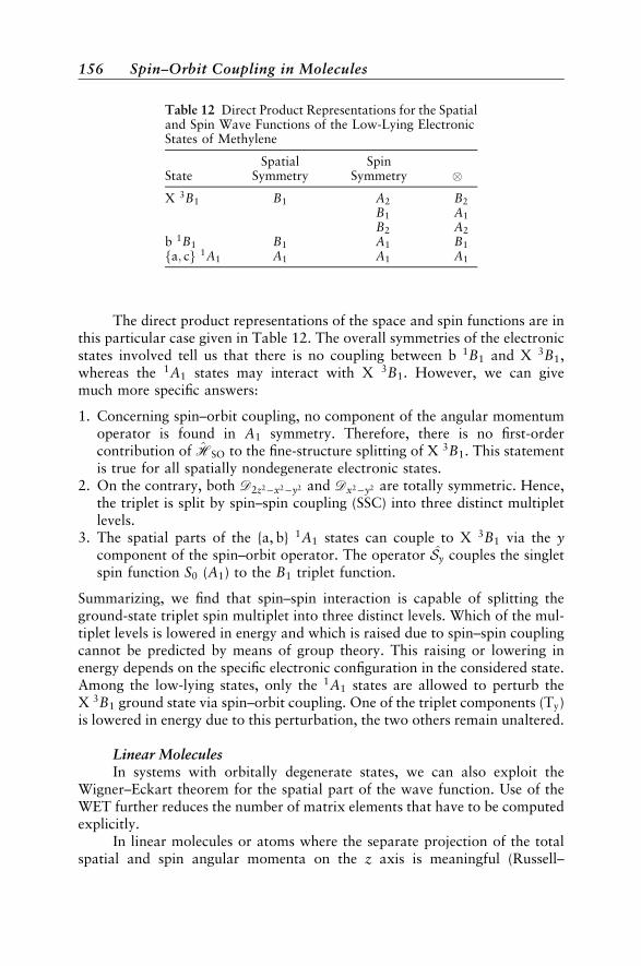
The direct product representations of the space and spin functions are inthis particular case given in Table 12. The overall symmetries of the electronicstates involved tell us that there is no coupling between b 1B1 and X 3B1,whereas the 1A1 states may interact with X 3B1. However, we can givemuch more specific answers:

1. Concerning spin–orbit coupling, no component of the angular momentumoperator is found in A1 symmetry. Therefore, there is no first-ordercontribution of HSO to the fine-structure splitting of X 3B1. This statementis true for all spatially nondegenerate electronic states.

2. On the contrary, both D2z2x2y2 and Dx2y2 are totally symmetric. Hence,the triplet is split by spin–spin coupling (SSC) into three distinct multipletlevels.

3. The spatial parts of the a, b 1A1 states can couple to X 3B1 via the ycomponent of the spin–orbit operator. The operator Sy couples the singletspin function S0 (A1) to the B1 triplet function.

Summarizing, we find that spin–spin interaction is capable of splitting theground-state triplet spin multiplet into three distinct levels. Which of the mul-tiplet levels is lowered in energy and which is raised due to spin–spin couplingcannot be predicted by means of group theory. This raising or lowering inenergy depends on the specific electronic configuration in the considered state.Among the low-lying states, only the 1A1 states are allowed to perturb theX 3B1 ground state via spin–orbit coupling. One of the triplet components (Ty)is lowered in energy due to this perturbation, the two others remain unaltered.

Linear MoleculesIn systems with orbitally degenerate states, we can also exploit the

Wigner–Eckart theorem for the spatial part of the wave function. Use of theWET further reduces the number of matrix elements that have to be computedexplicitly.

In linear molecules or atoms where the separate projection of the totalspatial and spin angular momenta on the z axis is meaningful (Russell–

Table 12 Direct Product Representations for the Spatialand Spin Wave Functions of the Low-Lying ElectronicStates of Methylene

Spatial SpinState Symmetry Symmetry X 3B1 B1 A2 B2

B1 A1

B2 A2

b 1B1 B1 A1 B1

fa; cg 1A1 A1 A1 A1

156 Spin–Orbit Coupling in Molecules

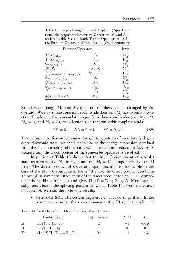
Saunders coupling), ML and MS quantum numbers can be changed by theoperator HSO by at most one unit each, while their sum MJ has to remain con-stant. Employing the nomenclature specific to linear molecules (i.e., MJ ¼ ,ML ¼ , and MS ¼ ), the selection rule for spin–orbit coupling reads:

¼ 0 ¼ 0;1 ¼ 0;1 ½189

To determine the first-order spin–orbit splitting pattern of an orbitally degen-erate electronic state, we shall make use of the energy expression obtainedfrom the phenomenological operator, which in this case reduces to ASO because only the z component of the spin–orbit operator is involved.

Inspection of Table 13 shows that the MS ¼ 0 component of a tripletstate transforms like in C1v, and the MS ¼ 1 components like the irrep. The direct product of space and spin functions is irreducible in thecase of the MS ¼ 0 component. For a 3 state, the direct product results inan overall symmetry. Reduction of the direct product for MS ¼ 1 compo-nents is readily carried out and gives ¼ þ . More specifi-cally, one obtains the splitting pattern shown in Table 14. From the entriesin Table 14, we read the following results:

" First-order SOC lifts certain degeneracies but not all of them. In theparticular example, the six components of a 3 state are split into

Table 13 Irreps of Singlet (S) and Triplet (T) Spin Func-

tions, the Angular Momentum Operators ( ~L and~S),

an Irreducible Second-Rank Tensor Operator D, andthe Position Operators XYZ in C1v ðD1hÞ Symmetry

Function/Operator Irrep.

TripletMS¼0 T0 ðgÞTripletMS¼1 T1 ðgÞSingletMS¼0 S0 þðgÞLz; Sz L0; S0 ðgÞLðxiyÞ=

ffiffi2p ; SðxiyÞ=

ffiffi2p L1; S1 ðgÞ

Dð2z2x2y2Þ=ffiffi6p D0 þðgÞ

DðxzþzxiðyzþzyÞÞ=2 D1 ðgÞDðx2y2iðxyþyxÞÞ=2 D2 ðgÞZ T0 þðuÞðX iYÞ=

ffiffiffi2p

T1 ðuÞ

Table 14 First-Order Spin–Orbit Splitting of a 3 State

Product State jj ¼ j þ j E

þ1Tþ1; 1T1 2 þ1 þASO

þ1T0; 1T0 1 0 0

ð1=ffiffiffi2pÞ½þ1T1 1Tþ1 0 1 ASO

Symmetry 157

three doubly degenerate levels. (We should point out that a degeneracyof the 0 levels is not required by group theory. The S1Dþ2S1 andSþ1D2Sþ1 components of the electronic spin–spin coupling operatorand higher-order SOC lift their degeneracy. It requires a different typeof interaction, that is, either the coupling to an external magnetic fieldor the rotation of the nuclear framework to split also the ¼ 2 and ¼ 1 sublevels.)

" There is a first-order splitting pattern common to all 3 states,independent of the physical content. All the molecule-dependentphysical information is contained in the parameter ASO. These factsare, of course a consequence of the tensor properties expressed in theWigner–Eckart theorem.

Summary

1. Only in spatially degenerate states, HSO may cause a multiplet splitting infirst order.

2. The operator HSO couples states of different spin and space symmetries insecond order, independent of spatial degeneracies.

3. It is possible to use the Wigner–Eckart theorem for reducing the number ofmatrix elements that have to be calculated. Symmetry rules can be obtainedfrom the tensorial structure of the interaction Hamiltonians.

4. As a consequence of the WET, there is a first-order splitting patterncommon to all states of a specific space þ spin symmetry, independent ofthe physical content.

5. Double groups: For describing the transformation properties of the a and bspin functions, it is necessary to augment the ordinary molecular pointgroup by symmetry operations that result from multiplying the originalsymmetry operations by a rotation through 2p. The resulting enlargedpoint groups are called double groups.

6. Many-particle spin functions:Odd number of electrons ! Fermion irreps of the double groupEven number of electrons ! Boson irreps of the double group

7. Selection rules for HSO ( !: coupling allowed; n!: no interaction; usignifies ungerade states)a. Systems with an inversion center strictly: g !g; u !u; g n! ub. Atoms strictly: dJJ 0 , dMJM 0

J

LS coupling: Lþ L0 1 jL L0j; S0 þ S 1 jS0 Sjc. Linear molecules strictly: ¼ 0

LS coupling: ¼ 0;1; ¼ 0;1; S0 þ S 1 jS0 Sjd. Nonlinear molecules strictly: refer to direct product representations of

the appropriate double group.LS coupling: S; S0 as above

158 Spin–Orbit Coupling in Molecules

COMPUTATIONAL ASPECTS

General Considerations

Various approaches can be pursued to compute spin–orbit effects. Four-component ab initio methods automatically include scalar and magnetic rela-tivistic corrections, but they put high demands on computer resources. (Forreviews on this subject, see, e.g., Refs. 18,19,81,82.) The following discussionfocuses on two-component methods treating SOC either perturbationally orvariationally. Most of these procedures start off with orbitals optimized fora spin-free Hamiltonian. Spin–orbit coupling is added then at a later stage.The latter approaches can be divided again into so-called one-step or two-step procedures as explained below.

In light molecules, SOC predominantly affects spectral properties such asfine-structure and transition probabilities. Fine-structure splittings originateboth from first- and higher-order spin–orbit contributions. In the languageof magnetic resonance, these are also dubbed diamagnetic and paramagneticcontributions, respectively. The latter depend both on spin–orbit couplingmatrix elements and on spin-free energy differences. Independent of thespin–orbit interaction scheme, it is therefore indispensable to employ methodsthat take electron correlation into account.

In heavy element compounds, spin–orbit interaction is of concern alsofor binding energies because the mutual spin–orbit interaction between mole-cular states will in general be smaller than in the dissociation limit. (Sometimesthis is also addressed as quenching of SOC, although the interaction does notdisappear completely.) Those molecular states that correlate with the lowerspin–orbit component of a heavy element atomic state will therefore bemore loosely bound. In contrast, the states that dissociate to the upper atomicspin–orbit level are stabilized by SOC.

Approximately from the 3d elements onward, it is necessary to add spin-independent (scalar) relativistic corrections to the Hamiltonian.18 In earlyworks, the differential scalar relativistic effect to molecular excitation energieswas often estimated by adding mass–velocity and Darwin corrections14 pertur-bationally. However, even for first- and second-row transition metals, itturned out that scalar relativistic effects are preferably taken into accountduring the orbital optimization,83,84 whereas this is mandatory for heavier ele-ment compounds.85 In two-component methods, integrals including kinematicrelativistic corrections can be generated either by utilizing relativistic effectivecore potentials (see, e.g., Refs. 35,37,38) or by employing a one-componentrelativistic all-electron Hamiltonian that is bounded from below. An overviewover state-of-the-art one-component relativistic electronic structure methodshas recently been given by Hess and Marian.19

Different computational strategies ought to be pursued for heavy maingroup elements and transition metals:

Computational Aspects 159

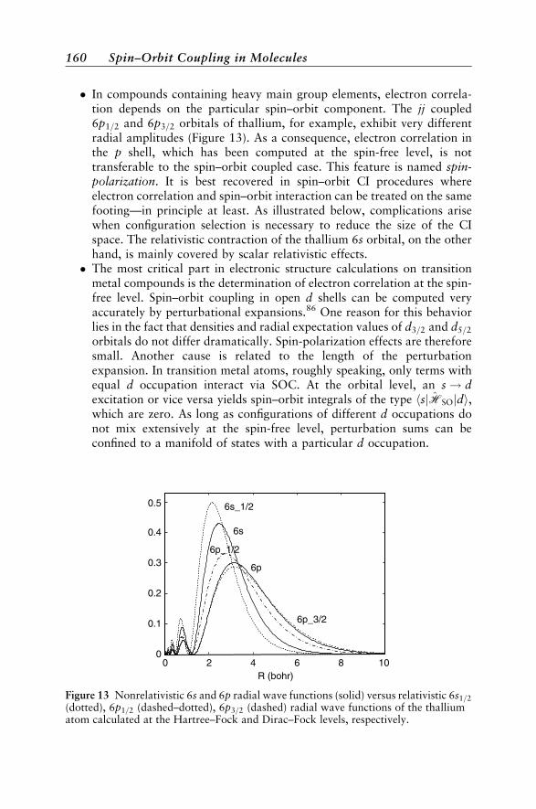
* In compounds containing heavy main group elements, electron correla-tion depends on the particular spin–orbit component. The jj coupled6p1=2 and 6p3=2 orbitals of thallium, for example, exhibit very differentradial amplitudes (Figure 13). As a consequence, electron correlation inthe p shell, which has been computed at the spin-free level, is nottransferable to the spin–orbit coupled case. This feature is named spin-polarization. It is best recovered in spin–orbit CI procedures whereelectron correlation and spin–orbit interaction can be treated on the samefooting—in principle at least. As illustrated below, complications arisewhen configuration selection is necessary to reduce the size of the CIspace. The relativistic contraction of the thallium 6s orbital, on the otherhand, is mainly covered by scalar relativistic effects.

* The most critical part in electronic structure calculations on transitionmetal compounds is the determination of electron correlation at the spin-free level. Spin–orbit coupling in open d shells can be computed veryaccurately by perturbational expansions.86 One reason for this behaviorlies in the fact that densities and radial expectation values of d3=2 and d5=2

orbitals do not differ dramatically. Spin-polarization effects are thereforesmall. Another cause is related to the length of the perturbationexpansion. In transition metal atoms, roughly speaking, only terms withequal d occupation interact via SOC. At the orbital level, an s! dexcitation or vice versa yields spin–orbit integrals of the type hsjHSOjdi,which are zero. As long as configurations of different d occupations donot mix extensively at the spin-free level, perturbation sums can beconfined to a manifold of states with a particular d occupation.

0

0.1

0.2

0.3

0.4

0.5

0 2 4 6 8 10R (bohr)

6s_1/2

6s

6p_1/2

6p

6p_3/2

Figure 13 Nonrelativistic 6s and 6p radial wave functions (solid) versus relativistic 6s1=2

(dotted), 6p1=2 (dashed–dotted), 6p3=2 (dashed) radial wave functions of the thalliumatom calculated at the Hartree–Fock and Dirac–Fock levels, respectively.

160 Spin–Orbit Coupling in Molecules

* Spin-polarization should also play a minor role in lanthanides andactinides. Differential correlation between states of different f occupa-tion and spin–orbit coupling within a given sldmf n manifold are huge,however. Further, the number of electronic states that can be derivedfrom an sldmf n occupation is in general too large for an explicitexpansion of the spin–orbit coupled states in unperturbed ones. In spiteof these difficulties, good progress has been made in recent years.56

We confine the discussion in the remainder of this section to the treat-ment of electronic wave functions. This confinement to electronic wave func-tions is justified as long as no (sharply avoided) intersystem crossings arepresent or other non-Born–Oppenheimer effects such as rovibronic (rota-tional/vibrational/electronic) coupling are involved. Intersystem crossingswill be discussed in connection to nonradiative transitions.

Evaluation of Spin–Orbit Integrals

Early implementations of Breit-Pauli spin–orbit integrals were based onSlater-type orbitals (STOs).63,87–90 All these programs involve numerical inte-gration schemes that become prohibitively expensive in polyatomic molecules.Kern and Karplus91 proposed a Gaussian transform for STOs, but explicit for-mulas were only given for s functions. For a while, Gaussian lobe functionswere popular because they are composed only of s functions.92–94 Besides sorbitals, p orbitals are easily described by linear combinations of lobe func-tions, but the extension to higher angular momentum basis functions leadsto numerical problems. King and Furlani95 derived formulas for evaluatingBreit-Pauli (BP) integrals in the basis of Cartesian Gaussians numerically bymeans of Rys quadrature techniques.

Actual computer codes for polyatomic molecules employ either Carte-sian or Hermite Gaussian functions. The calculation of all-electron spin–orbitintegrals makes use of second derivatives of Coulomb integrals with respect tonuclear coordinates.93,96–104 The relation between Coulomb and BP spin–obitintegrals is immediately apparent, if the BP operator is written as in expres-sions [101] and [102]. Instead of acting with r on 1=r in integrals ofrð1=rÞ r, the r on the left can be applied to the bra vector and the otherone to the ket vector. The derivative of an s function is a p function; taking thederivative of a p function yields an s and a d function, and so on. In this way,the spatial parts of a BP integral can be written as a linear combination ofCoulomb integrals.

The no-pair spin–orbit Hamiltonian [105] differs from the correspond-ing BP terms [103] by momentum dependent factors of the type Ai=ðEi þmc2Þ or ðAiAjÞ=ðEi þmec

2Þ, where Ei and Ai or Aj have been definedin [106] and [107], respectively. There are essentially two ways of taking thesefactors into account.

Computational Aspects 161

* The first was pioneered by Samzow et al.103 and makes use of a methodproposed by Hess for spin-independent one-electron no-pair operators.25

This approach resembles a resolution-of-the-identity ansatz. As thekinematical factors are functions of the momentum, they are most easilyevaluated in momentum space. The auxiliary basis set should span themomentum space as completely as possible. If the set of uncontractedfunctions is not sufficient for this purpose, it has to be augmented byfurther primitives. First, the spatial auxiliary basis functions areorthogonalized. The matrix of the nonrelativistic kinetic energy operatorp2

i =2me is diagonalized in a second step. Its eigenvectors form a discreterepresentation of the (continuous) spectrum of the momentum operator.If the basis were complete, then every other operator that can be writtenas a polynomial of the momentum would be diagonal. In a finite basis,this property is only approximately fulfilled. The eigenvectors of thekinetic energy matrix are utilized to evaluate the momentum dependentfactors in the no-pair Hamiltonian. The last step is a transformation backto the original auxiliary basis.

* The second way avoids transformations back and forth, which areparticularly time consuming for two-electron integrals. Almlof andco-workers105 noticed that kinematical factors such as Ai=ðEi þmec

2Þ orðAiAjÞ=ðEi þmec

2Þ can be turned over to the basis functions instead ofapplying them to the BP operator. Under certain circumstances, themodified basis functions can be reexpanded in the original basis so thatonly the contraction coefficients change. In this way, any program thatevaluates BP integrals can be utilized to compute approximate no-pairintegrals.

Effective core-potential [127] and atomic mean-field spin–orbit opera-tors [128] are in essence one-center operators. Only the projectors containmulticenter terms, but these yield merely overlap integrals. One-center spin–orbit integrals are therefore most easily evaluated in the basis of sphericalGaussians.64 The computation reduces then to a 1D radial integration andmultiplication by analytically determined factors from the angular part.Exploiting the spherical symmetry of the one-center terms thus appreciablyspeeds up the integral evaluation time and appears to be the only tractableway to perform all-electron spin–orbit calculations in large molecules. Forfurther usage in a molecular code, a basis set transformation to a Cartesianor so-called real spherical Gaussian basis is performed.f Atomic mean-field

fReal spherical Gaussian basis functions are not proper ‘z eigenfunctions. They are linearcombinations of spherical Gaussians expðar2Þ ðamY‘

m þ bmY‘mÞ with coefficients am

and bm chosen such that real basis functions result.

162 Spin–Orbit Coupling in Molecules

integrals for ab initio model potentials (AIMPs) are evaluated in an all-electronbasis first and are transferred then to the AIMP basis.65 A prerequisite for thisprocedure to work is an approximate matching of the respective valence orbi-tal exponents and contraction coefficients. Therefore, this approach shouldonly be applied in connection with generalized contracted basis sets of the Raf-fenetti or atomic natural orbital types.106,107

Perturbational Approaches to Spin–Orbit Coupling

As in all perturbational approaches, the Hamiltonian is divided into anunperturbed part Hð0Þ and a perturbation V. The operator Hð0Þ is a spin-free,one-component Hamiltonian and the spin–orbit coupling operator takes therole of the perturbation. There is no natural perturbation parameter l inthis particular case. Instead, HSO is assumed to represent a first-order pertur-bation Hð1Þ. The perturbational treatment of fine structure is an inherent two-step approach. It starts with the computation of correlated wave functions andenergies for pure spin states—mostly at the CI level. In a second step, spin–orbit perturbed energies and wavefunctions are determined.

Rayleigh–Schrodinger ExpansionIn Rayleigh–Schrodinger perturbation theory, perturbed wave functions

are expanded in the infinite set of eigenfunctions ð0Þ of the unperturbedHamiltonian. In practical applications, the sum over states is truncated to afinite number, of course. In principle, the eigenstates ð0Þ could be constructedfrom determinants using separate sets of molecular orbitals. Mutually non-orthogonal orbital bases add a complication to the evaluation of matrix ele-ments, in particular for two-electron operators, as the Slater–Condon rules[119] and [120] are not applicable right away. Formulas for self-consistentfield wave functions have been worked out by Bearpark et al.104 These involvebi-orthogonalization of the orbital sets and cofactors resulting from nonunityoverlaps. Employing different orbitals for different states (DODS) is desirablein many cases and certainly yields more accurate excitation energies than theuse of a common set of molecular orbitals (MOs), but the evaluation of spin–orbit matrix elements for general CI expansions is prohibitively expensive. Inmost cases, a common set of MOs is used as a one-particle basis for the con-struction of the determinants. Further, the order of the perturbation expansionis often confined to second order in the energy and to first order in the wavefunction.

A first-order contribution to the energy is obtained only for spatiallydegenerate states. Let us assume that the unperturbed state jð0Þk i has ad-fold degenerate eigenvalue, including both spin and space degeneracies.According to the rules of degenerate perturbation theory, the first-order

Computational Aspects 163

energies Eð1Þk;a are obtained by diagonalizing the interaction matrix in a basis

spanned by the d components jð0Þk;bi of jð0Þk i, where b is an index from 1 to d.

hð0Þk;1jHSOjð0Þk;1i hð0Þk;2jHSOjð0Þk;1i . . . hð0Þk;djHSOjð0Þk;1i

hð0Þk;1jHSOjð0Þk;2i hð0Þk;2jHSOjð0Þk;2i . . . hð0Þk;djHSOjð0Þk;2i

..

. ... . .

. ...

hð0Þk;1jHSOjð0Þk;di hð0Þk;2jHSOjð0Þk;di . . . hð0Þk;djHSOjð0Þk;di

0BBBBBB@

1CCCCCCA ½190

Only one of the matrix elements needs to be evaluated explicitly. All otherscan be obtained from the reduced matrix element by means of the Wigner–Eckart theorem, Eq. [166]. The eigenvectors

jð0Þk;ai ¼Xd

b¼1

jcð0Þk;a;bjð0Þk;bi ½191

are zeroth-order wave functions adapted to this particular perturbation.If the degeneracy is lifted completely in first-order or if at least second-

order effects do not introduce an additional splitting of degenerate levels, thesecond-order energy E

ð2Þk;l can be expressed as

Eð2Þk;a ¼

X1i 6¼k

Xd 0b0¼1

hð0Þk;ajHSOjð0Þi;b0 ihð0Þi;b0 jHSOjð0Þk;ai

Eð0Þi E

ð0Þk

½192

The corresponding first-order perturbed wave function reads

jð1Þk;ai ¼X1i 6¼k

Xd0b0¼1

hð0Þi;b0 jHSOjð0Þk;ai

Eð0Þi E

ð0Þk

jð0Þi;b0 i ½193

If these conditions are not fulfilled, an auxiliary condition is necessary to deter-mine the proper linear combinations of the jð0Þk;ai: although each set of ortho-gonal eigenfunctions qualifies as a proper wave function as long as thedegeneracy pertains, the wave function coefficients are required to changesmoothly when the additional perturbation is switched on adiabatically. Sym-metry properties of the involved states and operators may aid in predetermin-ing these linear combinations. In general, this procedure is too complicated,however, and one resorts to quasi-degenerate perturbation theory.

Moreover, first and second orders of perturbation theory are not definedin a stringent way in a molecule. Consider, for instance, all potential energycurves of a diatomic molecule that correspond to a specific dissociation

164 Spin–Orbit Coupling in Molecules

channel. Near the equilibrium geometry, the low-lying electronic states areusually well separated. Their mutual interaction is then described properlyby second-order perturbation theory. In the separated atom limit, first-orderdegenerate perturbation theory applies. In between, but still close to the disso-ciation limit, the states are nearly degenerate—or quasi-degenerate as wemight say. Neither of the procedures is then strictly applicable and orders ofperturbation theory are not well defined.

Quasi-Degenerate Perturbation TheoryAn often chosen way out of this dilemma is to set up a so-called pertur-

bation matrix in the basis of eigenvectors of a spin-free secular equation, mul-tiplied by an appropriate spin function. In this basis, matrix elements of thespin-free Hamiltonian occur only in the diagonal, of course. Due to symmetry,diagonal spin–orbit matrix elements come along only with complex wavefunctions. In a Cartesian basis, the integrals of the electrostatic Hamiltonianand the y component of HSO are real, whereas x and z integrals exhibit animaginary phase. (The spatial parts of the integrals are imaginary for all Car-tesian components. It is the choice of an imaginary phase for Sy that makes thematrix elements of the y component of HSO real.) As before, matrix elementsare computed only for one representative of a spin multiplet; all other matrixelements are generated by use of the WET.

Similar to first-order degenerate perturbation theory, perturbed energiesand wave functions are obtained by matrix diagonalization. This approach hastherefore been named quasi-degenerate perturbation theory. In spite of thisdesignation, the procedure is also applicable to states with large energy separa-tions. Other authors prefer to call it LS contracted spin–orbit configurationinteraction (SOCI) in order to stress its relation to configuration interactionprocedures in the limit of a complete set of eigenvectors.108 The perturbationmatrix is in most cases small enough for the application of standard complexHermitian eigenvalue and eigenvector solvers. Otherwise one can resort to thesame methods as in SOCI.

One of the great advantages of quasi-degenerate and Rayleigh–Schrodin-ger perturbation theories over SOCI procedures is that different levels ofsophistication can easily be mixed. For reasons of efficiency or technical lim-itations, it is in general not possible to a perform a full CI calculation thatyields the exact solution within a given basis set. Instead, configurations areselected according to some criterion such as excitation class or energy. Unfor-tunately, electron correlation contributions are slowly convergent. Further-more, truncated CI expansions are not size extensive, that is, the correlationenergy does not scale properly with the number of electrons. For spin-freestates, long-standing experience exists on how to estimate correlation contri-butions from discarded configurations or excitation classes.109–115 Theseextrapolated energies or the eigenvalues of correspondingly dressed Hamilto-nians can be taken as diagonal elements combined with spin–orbit matrix

Computational Aspects 165

elements of single excitation CI or smaller single and double excitation CIexpansions.41,108,116

A weakness of these methods lies in the limited number of zeroth-orderstates that are used for an expansion of the first-order perturbed wave func-tion. In particular, it has been demonstrated that probabilities of spin-forbid-den radiative transitions converge slowly with the length of the perturbationexpansion.92

Variational Perturbation and Response TheoryAs an alternative to sum-over-states methods, the perturbation equations

can be solved directly. In the context of spin–orbit coupling, reviews on thissubject have recently been given by Yarkony117 and by Agren et al.118

Hess et al.119 utilized a Hamiltonian matrix approach to determine thespin–orbit coupling between a spin-free correlated wave function and the con-figuration state functions (CSFs) of the perturbing symmetries. Havriliak andYarkony120 proposed to solve the matrix equation

ðHð0Þ Eð0Þi 1Þð1Þi ¼ HSO

ð0Þi ½194

directly for ð1Þi in the basis of CSFs. The direct solution of such a perturbation

equation is generally known as Hylleraas (or variational) perturbation th-eory.121,122 Yarkony123 developed this approach further by introducing a sym-bolic matrix element method, thereby extending the limits relating to thedimensionality of the Hamiltonian matrix.

Also in response theory the summation over excited states is effectivelyreplaced by solving a system of linear equations. Spin–orbit matrix elementsare obtained from linear response functions, whereas quadratic response func-tions can most elegantly be utilized to compute spin-forbidden radiative tran-sition probabilities. We refrain from going into details here, because anexcellent review on this subject has been published by Agren et al.118 Whilethese authors focus on response theory and its application in the frameworkof CI and multiconfiguration self-consistent field (MCSCF) procedures, ananalogous scheme using coupled-cluster electronic structure methods was pre-sented lately by Christiansen et al.124

Variational Procedures

For compounds containing heavy atoms, spin–orbit and electron correla-tion energies are approximately of the same size, and one cannot expect theseeffects to be independent of each other. A variational approach that treatsboth interactions at the same level is then preferable to a perturbation expan-sion. Special care is advisable in the choice of the spin–orbit operator in thiscase. The variational determination of spin–orbit coupling requires a spin–orbit

166 Spin–Orbit Coupling in Molecules

operator that is bounded from below such as the no-pair Hamiltonian,103 thezeroth-order regular approximation Hamiltonian (ZORA),125–127 or the ECPspin–orbit operators.39,40,52 Otherwise one has to constrain the basis set (e.g.,by an energy selection) to prevent a variational collapse.

jj Coupling MethodsTwo-component approaches employing one-particle spinors as basis

functions are referred to as jj coupling methods. They are typical one-step pro-cedures that take electron correlation and spin–orbit coupling into accountsimultaneously. Kramers-restricted two-component calculations at the Har-tree–Fock, second-order Møller-Plesset, singles and doubles CI, and coupledcluster levels have been reported for atoms and diatomic molecules.128,129

Technically Lee and co-workers utilized modified versions of four-componentprograms.130 Two-component wave function approaches that include SOCright away at the orbital optimization stage are rarely applied to moleculeswith more than two atoms. Possible reasons are the complications thatarise from a formulation of subsequent correlation treatments due tocomplex-valued orbital coefficients. Among the most widely used two-component methods in the field of chemistry are spin density functional meth-ods.131–133 In the Kohn–Sham approximation, complex orbital coefficientsemerge, but this is not problematic due to the restriction to a singledeterminant.

Intermediate Coupling ProceduresMost of the variational treatments of spin–orbit interaction utilize one-

component MOs as the one-particle basis. The SOC is then introduced at theCI level. A so-called SOCI can be realized either as a one- or two-step proce-dure. Evidently, one-step methods determine spin–orbit coupling and electroncorrelation simultaneously. In two-step procedures, typically different matrixrepresentations of the electrostatic and magnetic Hamiltonians are chosen.

In a one-step SOCI, a Hamiltonian matrix is set up in the basis of CSFsor determinants. It contains simultaneously matrix elements of the usual elec-trostatic Hamiltonian and of the spin–orbit operator and is complex in general.Since spin–orbit coupling mixes spin and spatial degrees of freedom, there arefewer possibilities of blocking the Hamiltonian matrix than for a spin-inde-pendent operator. To this end, one makes use of double group symmetriesand transforms the Cartesian basis functions to so-called Kramers pairs.52,134

By a special choice of phases, the matrix can even be made real in some cases.In general, however, very large complex eigenvalue problems have to be solvedin a SOCI.

Due to its dimensionality, a complete diagonalization of the CI matrix isnot feasible. One usually looks only for a few roots by means of an iterativeprocedure. For quantum chemical purposes, the Davidson algorithm ormodifications thereof have proven to be well suited.135–137 In its original

Computational Aspects 167

formulation, the Davidson method is applicable to real symmetric matricesonly. With some care, it can nevertheless be applied also to a complex eigen-value problem. Every complex Hermitian matrix C can be written as

C ¼ Aþ iB ½195

where A and B are real matrices. Since C is Hermitian, A is a symmetricmatrix, and B is skew symmetric.g Similarly, the eigenvectors ~Zi of C can bedivided into a real part ~Ui and an imaginary part i~Vi, where ~Vi itself is real.The complex eigenvalue problem

C~Zi ¼ Ei~Zi ½196

can then be replaced by a real symmetric eigenvalue problem of two times itsoriginal dimension.138

A B

B A

~Ui

~Vi

!¼ Ei

~Ui

~Vi

!½197

All eigenvalues Ei of the real eigenvalue problem [197] are doubly degenerate.This degeneracy is of purely technical origin and should not be confused withKramers degeneracy,139,140 which may occur in addition. (For instance, fourdegenerate roots are obtained for a doublet state, i.e., two for each Kramerslevel.) In addition to the transposed eigenvector ð~Ui

~ViÞt, a second one withstructure ð~Vi

~UiÞt is obtained. One of these solutions can be discarded. Alter-natively, root-homing procedures can be employed to avoid its evaluationright from the beginning.136,137

Older versions of SOCI programs are very I/O intensive because theyused to store the Hamiltonian matrix on disk and read it in every iterationstep.52,141 Integral-driven direct methods for spin–orbit coupling came up inthe mid 1980s123,142 following the original fomulation of direct CI methodsfor spin-independent Hamiltonians.143–146 Modern direct SOCI programscan easily handle several million determinants.108,147–151

The convergence of the iterative determination of eigenvalues and eigen-vectors is accelerated appreciably if spin–orbit CI and quasi-degenerate pertur-bation theory procedures are combined. To this end, the perturbation matrix isset up in the basis of the most important LS contracted CI vectors jð0;1Þm i. Thesolutions of this small eigenvalue problem

jð1;1Þk i ¼Xsf CI states

m

cð1;1Þkm j

ð0;1Þm i ½198

are then used to start up the Davidson iteration.

gA matrix B is said to be skew-symmetric if Bij ¼ Bji.

168 Spin–Orbit Coupling in Molecules

As the number of electrons increases, the dimension of the CI spacebecomes increasingly large, even if excitations are restricted to single and dou-ble replacements. Many approximate schemes to restrict the number of config-urations in a SOCI have been devised. The selected intermediate coupling CI(SICCI) code is an extension of the original COLUMBUS DGCI program andutilizes electrostatic and magnetic interactions as a selection criterion.152 TheSPDIAG program141 within the BNSOC package153 is based on the MRD-CIapproach. The latter makes use of a correlation energy criterion for configura-tion selection and estimates the contribution of the discarded configurations tothe spin-free correlated energy E

ð0;1Þm by means of Epstein–Nesbet perturbation

theory.111 If one assumes that the expansion [198] represents a decent approx-imation to the SOCI solution, the MRD-CI extrapolation scheme can easily beextended to the spin–orbit coupled case.154,155 Also other approaches towarda balanced treatment of spin–orbit interaction and electron correlation arebased on a manipulation of the spin-free energies and wave functions. Apure shift of excitation energies in the Davidson135 start-up matrix is not suf-ficient, because the original eigenvalues of Hð0Þ are restored during the iterativeprocess.141 In the so-called spin-free state shifted (SFSS) SOCI method, thisproblem is circumvented by introducing a projector on the set of

ð0;1Þm .156

HsfssSO ¼ HSO þ

Xsf CI states

m

Emjð0;1Þm ihð0;1Þm j ½199

with

Em ¼ ðEm EXÞ ðEð0;1Þm Eð0;1ÞX Þ ½200

The Em quantities shift the spin-free excitation energies ðEð0;1Þm Eð0;1ÞX Þ, calcu-

lated at a lower level of correlation treatment, to the exact values ðEm EXÞor at least to higher accuracy estimates. Herein, X denotes a common refer-ence state, in general the electronic ground state.

Due to the structure of the spin–orbit Hamiltonian, off-diagonal blocksof the CI matrix are dominated by single excitations. On the other hand, forelectron correlation effects (diagonal blocks) double and higher excitations aredecisive. In many approximate schemes, this fact is exploited. One of the firstof these approaches was the relativistic CI (RCI) algorithm by Balasubrama-nian.157 This is a two-step procedure. In a first step, large-scale multiconfigura-tion SCF and multireference singles and doubles CI (MRSDCI) calculationsare carried out for a spin-free Hamiltonian to determine a set of natural orbi-tals (NOs). In the second step, spin–orbit interaction integrals are transformedto the NO basis and added to the one-electron Hamiltonian matrix elements ofa smaller, truncated MRSDCI in relativistic symmetries. DiLabio and Chris-tiansen158 studied the separability of spin–orbit and correlation energies for

Computational Aspects 169

sixth-row main group compounds. They propose to determine the energy shiftDSO

s due to spin–orbit coupling as the difference between spin-free and inter-mediate coupling single excitation CI calculations. The energy of the corre-lated spin–orbit coupled states is then estimated by summing DSO

s into thespin-free correlated energies Els

sd . Rakowitz et al.159 employed a SFSS SOCIapproach on the Irþ ion. They demonstrated that the heavily spin–orbit per-turbed spectrum of this ion can be obtained in good accord with experiment atthe single excitation level, if higher level correlated electrostatic energies areused to determine the shifts Em. Recently Vallet et al.160 extended the effectiveHamiltonian approach, originally implemented in the CIPSO code at the levelof quasi-degenerate perturbation theory,41 to be used in intermediate couplingcalculations. Instead of representing Heff

el þ HSO in the basis of LS contractedstates, the new effective and polarized spin–orbit CI (EPCISO) operates in adeterminantal model space. This model space is chosen as the union of theseparate reference spaces in nonrelativistic symmetries augmented by themost significant configurations contributing to either the correlation energyor spin–orbit coupling.

COMPARISON OF FINE-STRUCTURE SPLITTINGSWITH EXPERIMENT

Spectroscopic parameters of a molecule are derived from experimentallydetermined spectra by fitting term values to a properly chosen modelHamiltonian.161 Usually, the model Hamiltonian is an effective one-stateHamiltonian that incorporates the interactions with other electronic statesparametrically. In rare cases, experimentalists have used a multistate ansatzlike the supermultiplet approach162 to fit the rovibronic spectra of stronglyinteracting near-degenerate electronic states. The safest way of comparing the-oretical data to experiment is to compute the spectrum and to fit the calculatedterm energies to the same model Hamiltonian as the experimentalists use.

The vibrational dependence of an effective molecular parameter A isusually expressed as

Avi¼ Ae þ

Xk

ak vi þdi

2

k

½201

where Ae is the value of the property at the equilibrium distance, and di is thedegeneracy of the vibrational mode vi. The vibrational dependence is causedby the anharmonicity of the potential energy surface and by the variation of Awith the vibrational coordinate Q. Such information can in practice beobtained from a quantum chemical treatment only for diatomic and triatomicmolecules. To this end, A is fitted to a function of Q—mostly a polynomial or

170 Spin–Orbit Coupling in Molecules

a cubic spline—and vibrationally averaged, that is, AðQÞ is weighted with theprobability density of a particular vibrational state wvi

ðQÞ and integrated overthe vibrational coordinate Q

Avi¼ hwvi

ðQÞjAðQÞjwviðQÞi ½202

Alternatively, expectation values computed at the equilibrium geometry of agiven electronic state can be directly compared with experimental parametersextrapolated from rovibrational branches.

In many instances, the ‘‘fine-structure’’ splitting caused by (first-order)spin–orbit coupling is considerably larger than the energy separation betweenadjacent rotational levels—at least for low values of the total angular momen-tum J—and rotational excitations can thus be neglected in a first approxima-tion. Hydrides are exceptional in this respect because of their low reducedmasses and the resulting large rotational constants B. Methods for computingrovibrational spectra of diatomic molecules from ab initio data including spin–orbit and rotational coupling were proposed among others by Yarkony117 andby the author163 employing Hund’s case ðbÞ and ðaÞ basis functions, respec-tively.161 For a review on the theoretical determination of rovibronic spectraof triatomic molecules, please refer to the work of Peric et al.164 A generalexpression for the rotational dependence of a spectroscopic parameter cannotbe given. Its functional form varies with the type of basis functions chosen fordescribing the actual rotation of the nuclear frame; the choice of basis func-tions in turn depends on the order in which the angular momenta are coupled(Hund’s cases in linear molecules) and the type of rotor [spherical top, sym-metric top (prolate, oblate), asymmetric top]. Looking at these particular casesin detail goes far beyond the scope of the present chapter. For additional read-ing, see, for example, Refs. 165–167.

First-Order Spin–Orbit Splitting

Only spatially degenerate states exhibit a first-order zero-field splitting.This condition restricts the phenomenon to atoms, diatomics, and highly sym-metric polyatomic molecules. For a comparison with experiment, computedmatrix elements of one or the other microscopic spin–orbit Hamiltonianhave to be equated with those of a phenomenological operator. One has tobe aware of the fact, however, that experimentally determined parametersare effective ones and may contain second-order contributions. Second-orderSOC may be large, particularly in heavy element compounds. As discussed inthe next section, it is not always distinguishable from first-order effects.

A phenomenological spin–orbit Hamiltonian, formulated in terms oftensor operators, was presented already in the subsection on tensor operators.Few experimentalists utilize an effective Hamiltonian of this form (seeEq. [159]). Instead, shift operators are used to represent space and spin angular

Comparison of Fine-Structure Splittings with Experiment 171

momentum operators in their tensorial forms. Employing shift operator con-ventions and making use of the Russell–Saunders (LS) coupling scheme, thephenomenological spin–orbit Hamiltonian reads

ASO~L ~S ¼ akL0S0 þ

1

2a?ðLþS þ LSþÞ ½203

For the sign of the spin–orbit parameter ASO, the following conventionsapply:

* A positive ASO denotes a regular state (Figure 14). In regular states thesublevel with smallest J or quantum number is lowest in energy.

* A negative ASO denotes an inverted state (Figure 15). In inverted statesthe sublevel with largest J or quantum number is lowest in energy.

Typically, states with less than half-filled shells (particle states) are regular,whereas states with more than half-filled shells (hole states) are inverted.

Atoms: The Lande Interval RuleTo determine the first-order splitting pattern of an atomic state in terms

of the phenomenological spin–orbit parameter ASO [Eq. 203], we utilize

A SO > 0

A SO

Ω = 3/2

Ω = 1/2Figure 14 Spin–orbit splitting pattern of a(regular) 2r state. (The dashed line marksthe position of the unperturbed state.)

2A SO

2A SO

Ω = 1

Ω = 2

Ω = 3

A SO < 0Figure 15 Spin–orbit splitting pattern of an(inverted) 3i state.

172 Spin–Orbit Coupling in Molecules

Russell–Saunders coupling, that is,~J ¼ ð ~Lþ ~S Þ. From

~J 2 ¼ ð ~Lþ ~S Þ2 ¼

~L

2 þ 2L ~S þ S, we obtain

~L ~S ¼ 1

2ðJ2 L2 S2Þ ½204

Exploiting the fact that in first-order perturbation theory all sublevels exhibitidentical L2 and S2 eigenvalues, respectively, yields a spin–orbit splitting of

EðJÞ EðJ 1Þ ¼ ASOJ ½205

for two neighboring atomic fine-structure levels with quantum numbers J andJ 1. This expression is the famous Lande interval rule.

As an example where this rule can be applied favorably to determine anatomic spin–orbit parameter, consider the first excited state of atomic copper,2Dgðd9s2Þ. The 2Dg state of copper is well separated from other electronicstates that are allowed by symmetry to couple in second order. A 2D state givesrise to two fine-structure levels with total angular momentum quantum num-bers J ¼ 3

2 and J ¼ 52. The d9s2 configuration corresponds to a hole state, and

we therefore expect an inverted splitting pattern (Figure 16). From Lande’sinterval rule, we determine a splitting of 5

2 ASO. ASO may thus be calculateddirectly from the experimentally determined splitting168 of 2042 cm1 by mul-tiplying with 2

5, yielding ASO ¼ 816:8 cm1; this value is in good agreementwith the theoretically determined spin–orbit parameter of ASO ¼ 802:4cm1.169

Things are not as easy for the 3Dgðd9s1Þ ground state of nickel. From a3D atomic state, three fine-structure levels originate with total angular momen-tum quantum numbers J ¼ 1, J ¼ 2, and J ¼ 3 (Figure 17). The ratio of themeasured fine-structure splittings ½Eð2Þ Eð1Þ=½Eð3Þ Eð2Þ amounts to1.234 instead of 2

3 as expected from the Lande interval rule. The main causefor this deviation is an energy shift of the J ¼ 2 level due to the interactionwith neighboring states of the same angular momentum quantum number.The J ¼ 3 and J ¼ 1 levels of 3Dg are only weakly perturbed and their energyseparation, EðJ ¼ 3Þ EðJ ¼ 1Þ ¼ 5ASO, may be taken to extract anexperimental value for ASO ¼ 301:6 cm1. The experimental spin–orbitconstant is in excellent agreement with the theoretical value of 301 cm1.

5/2A SO

J = 3/2

J = 5/2Figure 16 Spin–orbit splitting pattern of aninverted 2D atomic state.

Comparison of Fine-Structure Splittings with Experiment 173

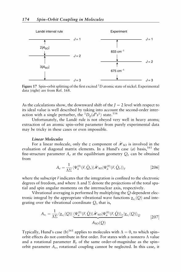
As the calculations show, the downward shift of the J ¼ 2 level with respect toits ideal value is well described by taking into account the second-order inter-action with a single perturber, the 1Dgðd9s1Þ state.116

Unfortunately, the Lande rule is not obeyed very well in heavy atoms;extraction of an atomic spin–orbit parameter from purely experimental datamay be tricky in these cases or even impossible.

Linear MoleculesFor a linear molecule, only the z component of HSO is involved in the

evaluation of diagonal matrix elements. In a Hund’s case (a) basis,161 thefine-structure parameter Ae at the equilibrium geometry Qe can be obtainedfrom

Ae ¼1

hð0Þn ð~r; ~QeÞjHSOjð0Þn ð~r; ~QeÞi~r ½206

where the subscript~r indicates that the integration is confined to the electronicdegrees of freedom, and where and denote the projections of the total spa-tial and spin angular momenta on the internuclear axis, respectively.

Vibrational averaging is performed by multiplying the Q-dependent elec-tronic integral by the appropriate vibrational wave functions wvi

ðQÞ and inte-grating over the vibrational coordinate Q, that is,

Avi ¼1

hwviðQÞj hð0Þn ð~r; ~QÞjHSOjð0Þn ð~r; ~QÞi~r|fflfflfflfflfflfflfflfflfflfflfflfflfflfflfflfflfflfflfflfflfflfflfflfflfflzfflfflfflfflfflfflfflfflfflfflfflfflfflfflfflfflfflfflfflfflfflfflfflfflffl jwvi

ðQÞiQ

ASOðQÞ½207

Typically, Hund’s case (b)161 applies to molecules with ¼ 0, to which spin–orbit effects do not contribute in first order. For states with a nonzero valueand a rotational parameter Bv of the same order-of-magnitdue as the spin–orbit parameter Av, rotational coupling cannot be neglected. In this case, it

3|ASO|

2|ASO|

Landé interval rule

J = 1

J = 2

J = 3

J = 1

J = 2

J = 3

675 cm−1

833 cm−1

Experiment

Figure 17 Spin–orbit splitting of the first excited 3D atomic state of nickel. Experimentaldata (right) are from Ref. 168.

174 Spin–Orbit Coupling in Molecules

appears most convenient to calculate the rovibrational spectrum in a Hund’scase (a) basis and to fit the fine-structure splittings to a function of the formg ~N ~S, where ~N represents the total angular momentum save for the spin andg is a proportionality factor. Examples for such a procedure may be found in astudy on the a3þ state of NOþ by Hutter et al.170 and in the work byKleinschmidt et al.171,172 who treat the fine-structure splitting of the X 2state of the CH radical in this way. Alternatively, Hund’s case (b) can beemployed.173

The strong coupling limit, Hund’s case (c)161, cannot be dealt with infirst order. Rather, it requires the inclusion of higher-order (at least second-order) spin–orbit coupling in the calculations.

Second-Order Spin–Orbit Splitting

Every electronic state of whatever spin or spatial symmetry may experi-ence an energy shift due to second-order spin–orbit effects. Singlet states aremerely shifted in one or the other direction depending on the relative energeticlocation of the perturber. In doublet states, second-order spin–orbit splittingjust adds to the first-order effect—in an atom or a nonrotating moleculethey cannot be distinguished experimentally. In triplets or higher multiplicitystates, second-order SOC causes deviations from the regular first-order split-ting patterns. These have been briefly addressed already in the section on Sym-metry and the section on First-Order Spin–Orbit Splitting. Unfortunately, it isnot possible to identify second-order SOC effects unambiguously solely on thebasis of experimental data, because second-order SOC and first-order electro-nic spin–spin coupling (SSC) have identical tensorial structures. To see this, werewrite the spin–orbit perturbation sum

X1n¼1

hð0Þ0 jHSOjnihnjHSOjð0Þ0 iEn E0

¼ hð0Þ0 jHSO

X1n¼1

jnihnjEn E0

!HSOjð0Þ0 i

½208

Further, HSO may be expressed formally as HSO ¼P

i~Qð1Þi ~si where the ~si

are the usual one-electron spin operators and the first rank tensor operators~Qð1Þi denote the spatial part of HSO related to electron i. (In the BP Hamil-

tonian (Eq. [104]), for example, ~Qð1Þi corresponds to the terms in braces.)

One then obtains

hð0Þ0 jX

i

~si~Qð1Þi

X1n¼1

jnihnjEn E0

!Xj

~Qð1Þj~sjjð0Þ0 i

¼ hð0Þ0 jX

i

Xj

~si~Qð1Þi

X1n¼1

jnihnjEn E0

!~Qð1Þj|fflfflfflfflfflfflfflfflfflfflfflfflfflfflfflfflfflfflfflfflfflzfflfflfflfflfflfflfflfflfflfflfflfflfflfflfflfflfflfflfflfflffl~sjjð0Þ0 i ½209

~Dð2Þij

Comparison of Fine-Structure Splittings with Experiment 175

The effective operator in Eq. [209] has exactly the same structure as the secondterm of the Breit-Pauli SSC operator in Eq. [162]. The fine-structure tensor ofrank two Dð2Þ has thus two major contributions

Dð2Þ ¼ Dð2ÞSS þD

ð2ÞSO ½210

In spatially nondegenerate states of light molecules such as the X 3 groundstate of O2, first-order SSC and second-order SOC have the same order ofmagnitude. However, spin–spin coupling involves only valence orbitals; con-tributions of closed-shell core orbitals cancel. This situation is not the case forspin–orbit coupling (see the section on Computational Aspects). As a conse-quence, SSC contributions remain nearly constant with growing nuclearcharge, whereas SOC increases considerably. In heavy element components,second-order SOC by far outweighs first-order SSC.

For a comparison with experimentally determined parameters, the calcu-lated total (SO and SS) Dð2Þ is equated with D

ð2ÞSS as used in the phenomeno-

logical electronic spin–spin operator, Eq. [164].In low-symmetry molecules, diagonal and off-diagonal matrix elements

of the electronic dipolar coupling tensor may contribute to hð0Þ0 jHSSjð0Þ0 i.Therefore, they are specified mostly in terms of their Cartesian components.If symmetry is C2v or higher, the off-diagonal matrix elements of the tensoroperator in Eq. [163] vanish (i.e., the principal axes diagonalizing the SCC ten-sor coincide with the inertial axes). For triplet and higher multiplicity states,one then obtains

hð0Þ0 jHSSjð0Þ0 i ¼ DxxS2x DyyS2

y DzzS2z ½211

Reordering and making use of the traceless property Dxx þDyy þDzz ¼ 0gives

hð0Þ0 jHSSjð0Þ0 i ¼ D S2z

1

3S2

þ EðS2

x S2yÞ ½212

where D and E are defined as

D ¼ 3

2Dzz ½213

E ¼ 1

2ðDyy DxxÞ ½214

Usually, experimentalists fit spin–spin splittings in terms of these parameters Dand E. For linear molecules, E ¼ 0 by symmetry, since Dyy ¼ Dxx. In theexperimental literature, a different notation (lSS) is sometimes used in this

176 Spin–Orbit Coupling in Molecules

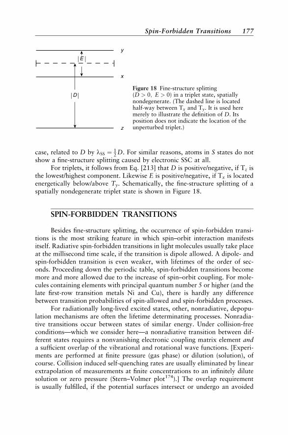
case, related to D by lSS ¼ 12 D. For similar reasons, atoms in S states do not

show a fine-structure splitting caused by electronic SSC at all.For triplets, it follows from Eq. [213] that D is positive/negative, if Tz is

the lowest/highest component. Likewise E is positive/negative, if Tx is locatedenergetically below/above Ty. Schematically, the fine-structure splitting of aspatially nondegenerate triplet state is shown in Figure 18.

SPIN-FORBIDDEN TRANSITIONS

Besides fine-structure splitting, the occurrence of spin-forbidden transi-tions is the most striking feature in which spin–orbit interaction manifestsitself. Radiative spin-forbidden transitions in light molecules usually take placeat the millisecond time scale, if the transition is dipole allowed. A dipole- andspin-forbidden transition is even weaker, with lifetimes of the order of sec-onds. Proceeding down the periodic table, spin-forbidden transitions becomemore and more allowed due to the increase of spin–orbit coupling. For mole-cules containing elements with principal quantum number 5 or higher (and thelate first-row transition metals Ni and Cu), there is hardly any differencebetween transition probabilities of spin-allowed and spin-forbidden processes.

For radiationally long-lived excited states, other, nonradiative, depopu-lation mechanisms are often the lifetime determinating processes. Nonradia-tive transitions occur between states of similar energy. Under collision-freeconditions—which we consider here—a nonradiative transition between dif-ferent states requires a nonvanishing electronic coupling matrix element anda sufficient overlap of the vibrational and rotational wave functions. [Experi-ments are performed at finite pressure (gas phase) or dilution (solution), ofcourse. Collision induced self-quenching rates are usually eliminated by linearextrapolation of measurements at finite concentrations to an infinitely dilutesolution or zero pressure (Stern–Volmer plot174).] The overlap requirementis usually fulfilled, if the potential surfaces intersect or undergo an avoided

E

D

y

x

z

Figure 18 Fine-structure splitting(D > 0; E > 0) in a triplet state, spatiallynondegenerate. (The dashed line is locatedhalf-way between Tx and Ty. It is used heremerely to illustrate the definition of D. Itsposition does not indicate the location of theunperturbed triplet.)

Spin-Forbidden Transitions 177

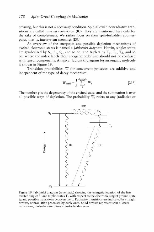
crossing, but this is not a necessary condition. Spin-allowed nonradiative tran-sitions are called internal conversion (IC). They are mentioned here only forthe sake of completeness. We rather focus on their spin-forbidden counter-parts, that is, intersystem crossings (ISC).

An overview of the energetics and possible depletion mechanisms ofexcited electronic states is named a Jablonski diagram. Herein, singlet statesare symbolized by S0, S1, S2, and so on, and triplets by T0, T1, T2, and soon, where the index labels their energetic order and should not be confusedwith tensor components. A typical Jablonski diagram for an organic moleculeis shown in Figure 19.

Transition probabilities W for concurrent processes are additive andindependent of the type of decay mechanism:

Wtotal ¼1

g

Xchannels

i

Wi ½215

The number g is the degeneracy of the excited state, and the summation is overall possible ways of depletion. The probability Wi refers to any (radiative or

Ene

rgy

S1

T1

S0

IC ISC

ISC

Figure 19 Jablonski diagram (schematic) showing the energetic location of the firstexcited singlet S1 and triplet states T1 with respect to the electronic singlet ground stateS0 and possible transitions between them. Radiative transitions are indicated by straightarrows, nonradiative processes by curly ones. Solid arrows represent spin-allowedtransitions, dashed–dotted lines spin-forbidden ones.

178 Spin–Orbit Coupling in Molecules

nonradiative) depletion mechanism. Since lifetime and transition probabilitiesare related by t ¼ 1=W, the total lifetime of an excited state is given by

1

ttotal¼ g

Xchannels

i

1

ti½216

This relationship means that the fastest process dominates the decay rate of anexcited state, and the fastest is very often a nonradiative transition.

Whether transitions from the spin–orbit split components of an electro-nic state can be observed individually depends on the size of the fine-structuresplitting and on the temperature. For large splittings and very low tempera-tures (usually below 10 K), transition probabilities are determined separatelyfor the multiplet components. In this case, the components are treated as non-degenerate levels (g ¼ 1). For closely spaced fine-structure levels, spin–latticerelaxation mechanisms cause a spin-depolarization at elevated temperatures.In the high-temperature limit—for organic molecules the temperature of liquidnitrogen (77 K) is usually sufficient—all fine-structure components are equallypopulated. Their individual transition probabilities have to be averaged then(degeneracy g ¼ 2Sþ 1). In between, a Boltzmann distribution can be used toestimate the population of the individual levels.

Radiative Transitions

A typical spin–forbidden radiative transition is the phosphorescencefrom the first excited triplet state to the singlet ground state of an organicmolecule. Another well-known example for a spin-forbidden radiative transi-tion concerns singlet oxygen. Singlet oxygen is long-lived and can be consid-ered as metastable with respect to the triplet ground state. Spin-forbiddenradiative transitions may occur also between doublet and quartet states.Chemists are less aware of those transitions because only a few stable mole-cules such as NO exist with an unpaired number of electrons.

Spin–Orbit Perturbed Wave FunctionsTo work out the fundamentals, we employ Rayleigh–Schrodinger pertur-

bation theory and restrict ourselves to a few terms in the (in principle) infiniteperturbation sums [193] because things are more transparent in this way. Inan actual calculation, it is more advantageous to use methods that avoid anexplicit summation over states, such as spin–orbit CI,41,52,117,141,147,160 varia-tional perturbation theory,119,120,123 or response theory.118,124,175 Excellentreviews on the latter two subjects have been given by Yarkony117 and by Agrenet al.118 We therefore refrain from going into the details of these methods.

As an example, we investigate the spin-forbidden transition from anexcited triplet (a) to a singlet electronic ground state (X). The resulting expres-sions can easily be extended to other cases, however. Let denote a spin–orbitcoupled state and a pure LS state. We express the unperturbed wave

Spin-Forbidden Transitions 179

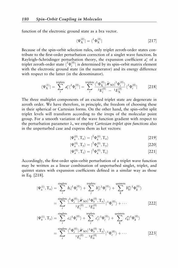
function of the electronic ground state as a bra vector.

hð0ÞX j ¼ h1ð0ÞX j ½217

Because of the spin–orbit selection rules, only triplet zeroth-order states con-tribute to the first-order perturbation correction of a singlet wave function. InRayleigh–Schrodinger perturbation theory, the expansion coefficient ai of atriplet zeroth-order state h3ð0Þi j is determined by its spin–orbit matrix elementwith the electronic ground state (in the numerator) and its energy differencewith respect to the latter (in the denominator).

hð1ÞX j ¼Xtriplets

i

ai h3ð0Þi j ¼

Xtriplets

i

h1ð0ÞX jHSOj3ð0Þi i3Eð0Þi 1E

ð0ÞX

h3ð0Þi j ½218

The three multiplet components of an excited triplet state are degenerate inzeroth order. We have therefore, in principle, the freedom of choosing thesein their spherical or Cartesian forms. On the other hand, the spin–orbit splittriplet levels will transform according to the irreps of the molecular pointgroup. For a smooth variation of the wave function gradient with respect tothe perturbation parameter l, we employ Cartesian triplet spin functions alsoin the unperturbed case and express them as ket vectors:

jð0Þa ;Txi ¼ j3ð0Þa ;Txi ½219jð0Þa ;Tyi ¼ j3ð0Þa ;Tyi ½220jð0Þa ;Tzi ¼ j3ð0Þa ;Tzi ½221

Accordingly, the first-order spin–orbit perturbation of a triplet wave functionmay be written as a linear combination of unperturbed singlet, triplet, andquintet states with expansion coefficients defined in a similar way as thosein Eq. [218].

jð1Þa ;Txi ¼Xsinglets

i

bij1ð0Þi i þXtriplets

j

b0jj3ð0Þj i þ

Xquintets

k

b00kj5ð0Þk i

¼Xsinglets

i

h1ð0Þi jHSOj3ð0Þa ;Txi1Eð0Þi 3E

ð0Þa

j1ð0Þi i þ ½222

jð1Þa ;Tyi ¼Xsinglets

i

cij1ð0Þi i þXtriplets

j

c0jj3ð0Þj i þ

Xquintets

k

c00kj5ð0Þk i

¼Xsinglets

i

h1ð0Þi jHSOj3ð0Þa ;Tyi1Eð0Þi 3E

ð0Þa

j1ð0Þi i þ ½223

180 Spin–Orbit Coupling in Molecules

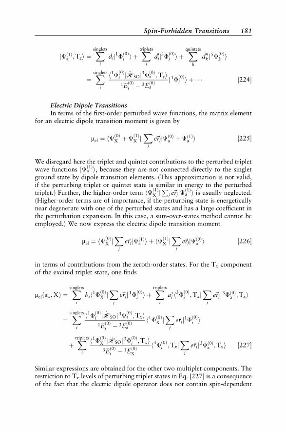
jð1Þa ;Tzi ¼Xsinglets

i

dij1ð0Þi i þXtriplets

j

d0jj3ð0Þj i þ

Xquintets

k

d00kj5ð0Þk i

¼Xsinglets

i

h1ð0Þi jHSOj3ð0Þa ;Tzi1Eð0Þi 3E

ð0Þa

j1ð0Þi i þ ½224

Electric Dipole TransitionsIn terms of the first-order perturbed wave functions, the matrix element

for an electric dipole transition moment is given by

mel ¼ hð0ÞX þ

ð1ÞX j

Xj

e~rjjð0Þa þð1Þa i ½225

We disregard here the triplet and quintet contributions to the perturbed tripletwave functions jð1Þa i, because they are not connected directly to the singletground state by dipole transition elements. (This approximation is not valid,if the perturbing triplet or quintet state is similar in energy to the perturbedtriplet.) Further, the higher-order term hð1ÞX j

Pj e~rjjð1Þa i is usually neglected.

(Higher-order terms are of importance, if the perturbing state is energeticallynear degenerate with one of the perturbed states and has a large coefficient inthe perturbation expansion. In this case, a sum-over-states method cannot beemployed.) We now express the electric dipole transition moment

mel ¼ hð0ÞX jX

j

e~rjjð1Þa i þ hð1ÞX jX

j

e~rjjð0Þa i ½226

in terms of contributions from the zeroth-order states. For the Tx componentof the excited triplet state, one finds

melðax;XÞ ¼Xsinglets

i

bih1ð0ÞX jX

j

e~rjj1ð0Þi i þXtriplets

i

ai h3ð0Þi ;Txj

Xj

e~rjj3ð0Þa ;Txi

¼Xsinglets

i

h1ð0Þi jHSOj3ð0Þa ;Txi1Eð0Þi 3E

ð0Þa

h1ð0ÞX jX

j

e~rjj1ð0Þi i

þXtriplets

i

h1ð0ÞX jHSOj3ð0Þi ;Txi3Eð0Þi 1E

ð0ÞX

h3ð0Þi ;TxjX

j

e~rjj3ð0Þa ;Txi ½227

Similar expressions are obtained for the other two multiplet components. Therestriction to Tx levels of perturbing triplet states in Eq. [227] is a consequenceof the fact that the electric dipole operator does not contain spin-dependent

Spin-Forbidden Transitions 181

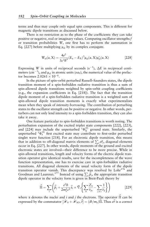
terms and thus may couple only equal spin components. This is different formagnetic dipole transitions as discussed below.

There is no restriction as to the phase of the coefficients: they can takepositive or negative, real or imaginary values. Computing oscillator strengths for transition probabilities W, one first has to perform the summation inEq. [227] before multiplying mel by its complex conjugate.

Welða;XÞ ¼4e2

3c3h4ðEa EXÞ3melða;XÞmelða;XÞ ½228

Expressing W in units of reciprocal seconds (s1), E in reciprocal centi-meters (cm1), and mel in atomic units (ea0), the numerical value of the prefac-tor becomes 2:0261 106.

In the picture of spin–orbit perturbed Russell–Saunders states, the dipoletransition moment of a spin-forbidden radiative transition is thus a sum ofspin-allowed dipole transitions weighted by spin–orbit coupling coefficients(e.g., the expansion coefficients in Eq. [218]). The fact that the transitiondipole moment of a spin-forbidden radiative transition is a weighted sum ofspin-allowed dipole transition moments is exactly what experimentalistsmean when they speak of intensity borrowing. The contribution of perturbingstates to the oscillator strength can be positive or negative. In other words, per-turbers can not only lend intensity to a spin-forbidden transition, they can alsotake it away.

One feature particular to spin-forbidden transitions is worth noting. Theperturbation expansion of the excited triplet state components [222], [223],and [224] may include the unperturbed 1

ð0ÞX ground state. Similarly, the

unperturbed 3ð0Þa first excited state may contribute to first-order perturbed

singlet wave function [218]. For an electronic dipole transition, this meansthat in addition to off-diagonal matrix elements of

Pj e~rj, diagonal elements

occur in Eq. [227]. In other words, dipole moments of the ground and excitedelectronic states are involved—their difference to be more precise. While inspin-allowed transitions, length and velocity forms of the electric dipole tran-sition operator give identical results, save for the incompleteness of the wavefunction representation, one has to exercise care in spin-forbidden radiativetransitions. All diagonal elements of the usual velocity form of the dipoletransition operator vanish. This discrepancy was resolved by Lohr176 andGoodman and Laurenzi.177 Instead of using

Pi~pi, the appropriate transition

dipole operator in the velocity form is given in Breit-Pauli theory by

~ ¼

Xi

~pi þe2h

2m2e c2

~si ~ri

Xa

Za

riaXj 6¼ i

1

rij

( ) !½229

where a denotes the nuclei and i and j the electrons. The operator ~ can be

expressed by the commutator ½H0 þ HSO;~r ¼ ðih=meÞ~. Thus e~r is a correct

182 Spin–Orbit Coupling in Molecules

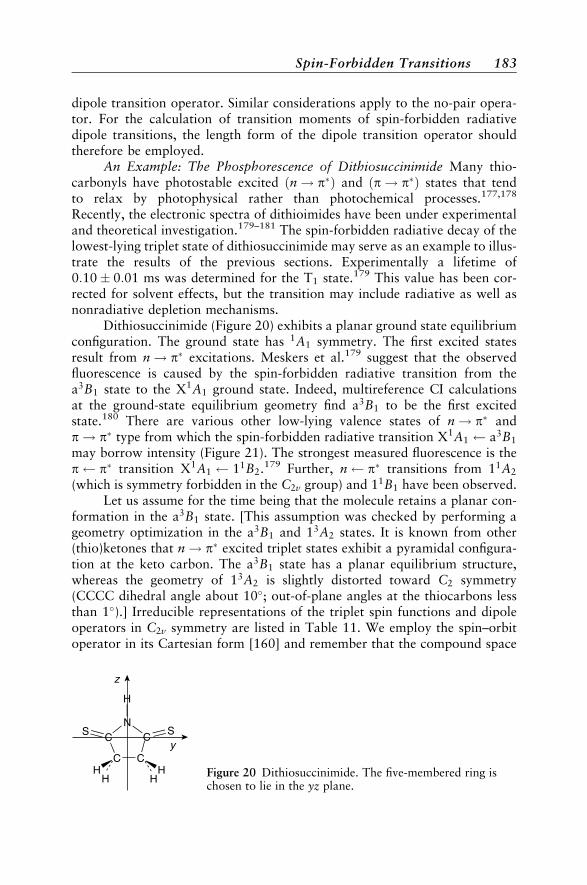
dipole transition operator. Similar considerations apply to the no-pair opera-tor. For the calculation of transition moments of spin-forbidden radiativedipole transitions, the length form of the dipole transition operator shouldtherefore be employed.

An Example: The Phosphorescence of Dithiosuccinimide Many thio-carbonyls have photostable excited ðn! pÞ and ðp! pÞ states that tendto relax by photophysical rather than photochemical processes.177,178

Recently, the electronic spectra of dithioimides have been under experimentaland theoretical investigation.179–181 The spin-forbidden radiative decay of thelowest-lying triplet state of dithiosuccinimide may serve as an example to illus-trate the results of the previous sections. Experimentally a lifetime of0:10 0:01 ms was determined for the T1 state.179 This value has been cor-rected for solvent effects, but the transition may include radiative as well asnonradiative depletion mechanisms.

Dithiosuccinimide (Figure 20) exhibits a planar ground state equilibriumconfiguration. The ground state has 1A1 symmetry. The first excited statesresult from n! p excitations. Meskers et al.179 suggest that the observedfluorescence is caused by the spin-forbidden radiative transition from thea3B1 state to the X1A1 ground state. Indeed, multireference CI calculationsat the ground-state equilibrium geometry find a3B1 to be the first excitedstate.180 There are various other low-lying valence states of n! p andp! p type from which the spin-forbidden radiative transition X1A1 a3B1

may borrow intensity (Figure 21). The strongest measured fluorescence is thep p transition X1A1 11B2.179 Further, n p transitions from 11A2

(which is symmetry forbidden in the C2v group) and 11B1 have been observed.Let us assume for the time being that the molecule retains a planar con-

formation in the a3B1 state. [This assumption was checked by performing ageometry optimization in the a3B1 and 13A2 states. It is known from other(thio)ketones that n! p excited triplet states exhibit a pyramidal configura-tion at the keto carbon. The a3B1 state has a planar equilibrium structure,whereas the geometry of 13A2 is slightly distorted toward C2 symmetry(CCCC dihedral angle about 10&; out-of-plane angles at the thiocarbons lessthan 1&).] Irreducible representations of the triplet spin functions and dipoleoperators in C2v symmetry are listed in Table 11. We employ the spin–orbitoperator in its Cartesian form [160] and remember that the compound space

C

CN

C

C

H

S S

HH H

H

z

y

Figure 20 Dithiosuccinimide. The five-membered ring ischosen to lie in the yz plane.

Spin-Forbidden Transitions 183

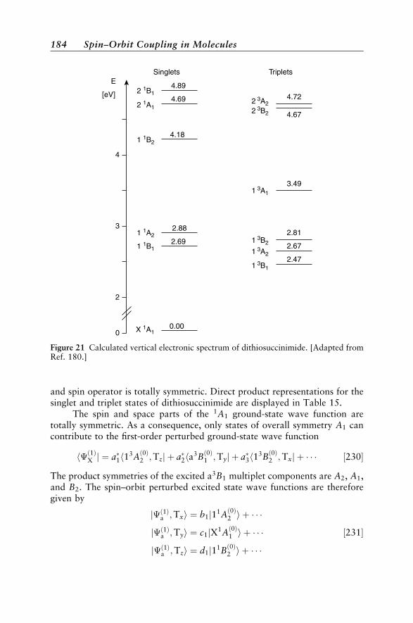
and spin operator is totally symmetric. Direct product representations for thesinglet and triplet states of dithiosuccinimide are displayed in Table 15.

The spin and space parts of the 1A1 ground-state wave function aretotally symmetric. As a consequence, only states of overall symmetry A1 cancontribute to the first-order perturbed ground-state wave function

hð1ÞX j ¼ a1h13Að0Þ2 ;Tzj þ a2ha3B

ð0Þ1 ;Tyj þ a3h13B

ð0Þ2 ;Txj þ ½230

The product symmetries of the excited a3B1 multiplet components are A2, A1,and B2. The spin–orbit perturbed excited state wave functions are thereforegiven by

jð1Þa ;Txi ¼ b1j11Að0Þ2 i þ

jð1Þa ;Tyi ¼ c1jX1Að0Þ1 i þ ½231

jð1Þa ;Tzi ¼ d1j11Bð0Þ2 i þ

2.69

2.88

4.18

4.69

4.89

0.00

2 1B1

2 1A1

1 1B2

1 1A2

1 1B1

X 1A1

2 3A22 3B2

1 3A1

1 3B2

1 3A2

1 3B12.47

2.67

2.81

3.49

4.67

4.72

2

E

3

4

0

[eV]

Singlets Triplets

Figure 21 Calculated vertical electronic spectrum of dithiosuccinimide. [Adapted fromRef. 180.]

184 Spin–Orbit Coupling in Molecules

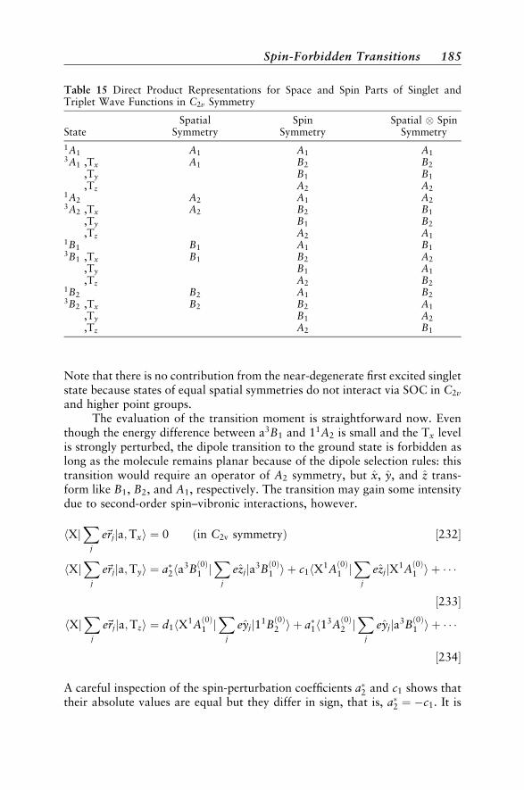
Note that there is no contribution from the near-degenerate first excited singletstate because states of equal spatial symmetries do not interact via SOC in C2v

and higher point groups.The evaluation of the transition moment is straightforward now. Even

though the energy difference between a3B1 and 11A2 is small and the Tx levelis strongly perturbed, the dipole transition to the ground state is forbidden aslong as the molecule remains planar because of the dipole selection rules: thistransition would require an operator of A2 symmetry, but x, y, and z trans-form like B1, B2, and A1, respectively. The transition may gain some intensitydue to second-order spin–vibronic interactions, however.

hXjX

j

e~rjja;Txi ¼ 0 ðin C2v symmetryÞ ½232

hXjX

j

e~rjja;Tyi ¼ a2ha3Bð0Þ1 jX

j

ezjja3Bð0Þ1 i þ c1hX1A

ð0Þ1 jX

j

ezjjX1Að0Þ1 i þ

½233

hXjX

j

e~rjja;Tzi ¼ d1hX1Að0Þ1 jX

j

eyjj11Bð0Þ2 i þ a1h13A

ð0Þ2 jX

j

eyjja3Bð0Þ1 i þ

½234

A careful inspection of the spin-perturbation coefficients a2 and c1 shows thattheir absolute values are equal but they differ in sign, that is, a2 ¼ c1. It is

Table 15 Direct Product Representations for Space and Spin Parts of Singlet andTriplet Wave Functions in C2v Symmetry

Spatial Spin Spatial SpinState Symmetry Symmetry Symmetry

1A1 A1 A1 A13A1 ,Tx A1 B2 B2

,Ty B1 B1

,Tz A2 A21A2 A2 A1 A23A2 ,Tx A2 B2 B1

,Ty B1 B2

,Tz A2 A11B1 B1 A1 B13B1 ,Tx B1 B2 A2

,Ty B1 A1

,Tz A2 B21B2 B2 A1 B23B2 ,Tx B2 B2 A1

,Ty B1 A2

,Tz A2 B1

Spin-Forbidden Transitions 185

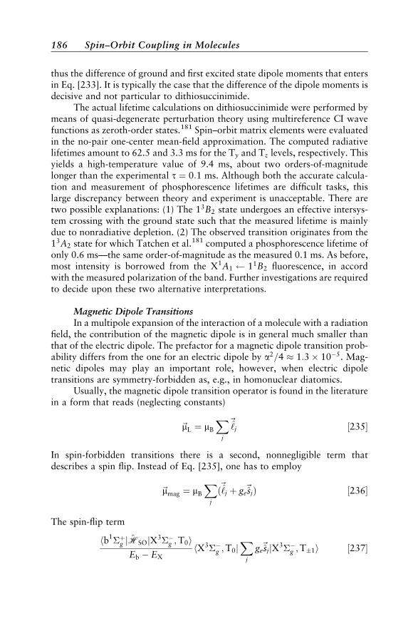
thus the difference of ground and first excited state dipole moments that entersin Eq. [233]. It is typically the case that the difference of the dipole moments isdecisive and not particular to dithiosuccinimide.

The actual lifetime calculations on dithiosuccinimide were performed bymeans of quasi-degenerate perturbation theory using multireference CI wavefunctions as zeroth-order states.181 Spin–orbit matrix elements were evaluatedin the no-pair one-center mean-field approximation. The computed radiativelifetimes amount to 62.5 and 3.3 ms for the Ty and Tz levels, respectively. Thisyields a high-temperature value of 9.4 ms, about two orders-of-magnitudelonger than the experimental t ¼ 0:1 ms. Although both the accurate calcula-tion and measurement of phosphorescence lifetimes are difficult tasks, thislarge discrepancy between theory and experiment is unacceptable. There aretwo possible explanations: (1) The 13B2 state undergoes an effective intersys-tem crossing with the ground state such that the measured lifetime is mainlydue to nonradiative depletion. (2) The observed transition originates from the13A2 state for which Tatchen et al.181 computed a phosphorescence lifetime ofonly 0.6 ms—the same order-of-magnitude as the measured 0.1 ms. As before,most intensity is borrowed from the X1A1 11B2 fluorescence, in accordwith the measured polarization of the band. Further investigations are requiredto decide upon these two alternative interpretations.

Magnetic Dipole TransitionsIn a multipole expansion of the interaction of a molecule with a radiation

field, the contribution of the magnetic dipole is in general much smaller thanthat of the electric dipole. The prefactor for a magnetic dipole transition prob-ability differs from the one for an electric dipole by a2=4 1:3 105. Mag-netic dipoles may play an important role, however, when electric dipoletransitions are symmetry-forbidden as, e.g., in homonuclear diatomics.

Usually, the magnetic dipole transition operator is found in the literaturein a form that reads (neglecting constants)

~mL ¼ mB

Xj

~‘j ½235

In spin-forbidden transitions there is a second, nonnegligible term thatdescribes a spin flip. Instead of Eq. [235], one has to employ

~mmag ¼ mB

Xj

ð~‘j þ ge~sjÞ ½236

The spin-flip term

hb1þg jHSOjX3g ;T0iEb EX

hX3g ;T0jX

j

ge~sjjX3g ;T1i ½237

186 Spin–Orbit Coupling in Molecules

was shown to make the major contribution to the transition probabilityb1þg ! X3g in O2.182,183

Again expressing W in units of reciprocal seconds ðs1Þ, E in reciprocalcentimeters ðcm1Þ, and mmag in atomic units (h), the probability of a magneticdipole transition from an initial state i to the final state f is given by

Wmagði; f Þ ¼ 2:6973 1011ðEi Ef Þ3mmagði; f Þmmagði; f Þ ½238

Nonradiative Transitions

Bound electronic states exhibit a discrete spectrum of rovibrationaleigenstates below the dissociation energy. The interaction between discretelevels of two bound electronic states may lead to perturbations in their rovi-brational spectra and to nonradiative transitions between the two potentials.In the case of an intersystem crossing, this process is often followed by a radia-tive depletion. Above the dissociation energy and for unbound states, theenergy is not quantized, that is, the spectrum is continuous. The coupling ofa bound state to the vibrational continuum of another electronic state leads topredissociation.

Apart from the selection rules for the electronic coupling matrix element,spin-forbidden and spin-allowed nonradiative transitions are treated com-pletely analogously. Nonradiative transitions caused by spin–orbit interactionare mostly calculated in the basis of pure spin Born–Oppenheimer states. Withrespect to spin–orbit coupling, this implies a diabatic behavior, meaning thatcurve crossings may occur in this approach. The nuclear Schrodinger equationis first solved separately for each electronic state, and the rovibronic states arespin–orbit coupled then in a second step.

In principle, static or dynamic approaches can be employed to describethe nonradiative transition between two states, although dynamic approachesare generally preferable. In a time-independent formalism, the coupling man-ifests itself in a mixing between vibrational levels of the involved electronicstates. The relative probability of finding the molecule in a particular state isproportional to its squared expansion coefficient. In the language of time-dependent perturbation theory, the coupling is expressed as a propagationback and forth between vibronic states. The equivalence between the staticand dynamic picture holds as long as there are no other fast depletion mechan-isms. In particular, the radiative lifetimes of the interacting states have to belong enough for an equilibration. If one of the states is short-lived, the nonra-diative transition occurs in essence only in one direction. The theory and com-putational treatment of the coupling between multidimensional potentialenergy surfaces have recently been reviewed by Koppel and Domcke.184

Here, we confine the discussion to cases that can be reduced to onedimension. As far as bound-continuum interactions are concerned, we restrictourselves to weak interactions. This condition is mostly fulfilled for

Spin-Forbidden Transitions 187

spin-forbidden processes. Otherwise the full apparatus of scattering theory hasto be invoked, which is far beyond the scope of this chapter.

Bound–Bound InteractionsPerturbations in the spectrum involving a pair of vibrationally bound

states occur only occasionally, for instance, when the vibrational ladders ofthe electronic states approximately match in energy. The mixing coefficientscan be calculated from the potential energy curves of the states involved andthe electronic coupling matrix element for various values of the vibrationalcoordinate. As noted previously, the Schrodinger equation for the vibrationalmotion is solved separately for each of the bound states. Their solutions aretaken as the basis for a matrix representation of the interaction Hamiltonian.To ease the integration over the vibrational coordinate Q, the electronic cou-pling matrix element X is often approximated by an analytic function of Q,mostly a polynomial or a cubic spline function. The matrix elements of theperturbation matrix are then calculated in a way similar to the vibrationalaveraging of spectroscopic parameters described in the previous section onthe Comparison of Fine-Structure Splittings with Experiment. Instead ofemploying the same vibronic level on both sides, now

Hij ¼ hwviðQÞjXðQÞjwv 0

jðQÞiQ ½239

is evaluated, where XðQÞ is the off-diagonal electronic coupling, and vi and v 0jbelong to different electronic states. Diagonalization of this matrix directlyyields energies and mixing coefficients of the levels.

In practical applications, one often combines experimental and theoreti-cal information. Potential energy curves, deduced from experiment with highaccuracy, if available, are employed together with theoretically determined Qdependent coupling matrix elements. As the degree of mixing between vibron-ic states strongly depends on their energetic separation, even uncertainties inthe electronic excitation energy of some 10 wavenumbers—which is a smallerror by present-day standards—are often sufficient to change the order-of-magnitude for a transition rate. Coupling matrix elements, on the otherhand, can be computed with high accuracy, whereas they are not really avail-able from experimental data.

From Eq. [239], it is apparent that the size of a particular Hij is not onlydetermined by the magnitude of the electronic coupling matrix element butalso by the overlap of the vibrational wave functions vi and v0j. Squared over-lap integrals of the type jhwvi

ðQÞjwv0jðQÞiQj

2 are frequently called Franck–Con-don (FC) factors. In contrast to radiative processes, FC factors fornonradiative transitions become particularly unfavorable if two states differ-ing considerably in their electronic energies exhibit similar shapes and equili-brium coordinates of their potential curves. Due to the near-degeneracyrequirement, an upper state vibrational wave function, with just a few nodes

188 Spin–Orbit Coupling in Molecules

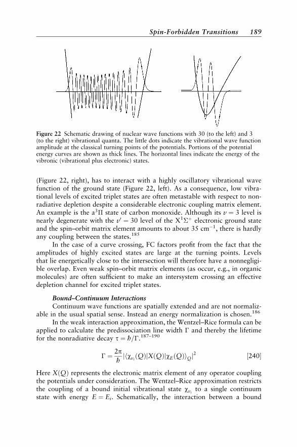
(Figure 22, right), has to interact with a highly oscillatory vibrational wavefunction of the ground state (Figure 22, left). As a consequence, low vibra-tional levels of excited triplet states are often metastable with respect to non-radiative depletion despite a considerable electronic coupling matrix element.An example is the a3 state of carbon monoxide. Although its v ¼ 3 level isnearly degenerate with the v0 ¼ 30 level of the X1þ electronic ground stateand the spin–orbit matrix element amounts to about 35 cm1, there is hardlyany coupling between the states.185

In the case of a curve crossing, FC factors profit from the fact that theamplitudes of highly excited states are large at the turning points. Levelsthat lie energetically close to the intersection will therefore have a nonnegligi-ble overlap. Even weak spin–orbit matrix elements (as occur, e.g., in organicmolecules) are often sufficient to make an intersystem crossing an effectivedepletion channel for excited triplet states.

Bound–Continuum InteractionsContinuum wave functions are spatially extended and are not normaliz-

able in the usual spatial sense. Instead an energy normalization is chosen.186

In the weak interaction approximation, the Wentzel–Rice formula can beapplied to calculate the predissociation line width and thereby the lifetimefor the nonradiative decay t ¼ h=.187–190

¼ 2phjhwviðQÞjXðQÞjwEðQÞiQj

2 ½240

Here XðQÞ represents the electronic matrix element of any operator couplingthe potentials under consideration. The Wentzel–Rice approximation restrictsthe coupling of a bound initial vibrational state wvi

to a single continuumstate with energy E ¼ Ei. Schematically, the interaction between a bound

Figure 22 Schematic drawing of nuclear wave functions with 30 (to the left) and 3(to the right) vibrational quanta. The little dots indicate the vibrational wave functionamplitude at the classical turning points of the potentials. Portions of the potentialenergy curves are shown as thick lines. The horizontal lines indicate the energy of thevibronic (vibrational plus electronic) states.

Spin-Forbidden Transitions 189

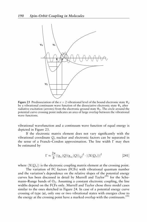
vibrational wavefunction and a continuum wave function of equal energy isdepicted in Figure 23.

If the electronic matrix element does not vary significantly with thevibrational coordinate Q, nuclear and electronic factors can be separated inthe sense of a Franck–Condon approximation. The line width may thenbe estimated by

2phjhwviðQÞjwvE

ðQÞiQj2 jhXðQxÞij2 ½241

where hXðQxÞi is the electronic coupling matrix element at the crossing point.The variation of FC factors (FCFs) with vibrational quantum number

and the variation’s dependence on the relative slopes of the potential energycurves has been discussed in detail by Murrell and Taylor191 for the Schu-mann–Runge bands of O2. Assuming a constant electronic coupling, the linewidths depend on the FCFs only. Murrell and Taylor chose three model casessimilar to the ones sketched in Figure 24. In case of a potential energy curvecrossing of type (a), only one or two vibrational states with energies close tothe energy at the crossing point have a marked overlap with the continuum.191

ψd ψk

ψ0

Figure 23 Predissociation of the v ¼ 2 vibrational level of the bound electronic state d

by a vibrational continuum wave function of the dissociative electronic state k afterradiative excitation (arrows) from the electronic ground state 0. The circle around thepotential curve crossing point indicates an area of large overlap between the vibrationalwave functions.

190 Spin–Orbit Coupling in Molecules

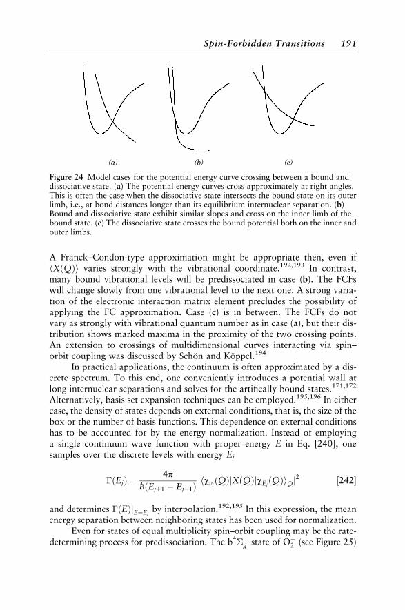
A Franck–Condon-type approximation might be appropriate then, even ifhXðQÞi varies strongly with the vibrational coordinate.192,193 In contrast,many bound vibrational levels will be predissociated in case (b). The FCFswill change slowly from one vibrational level to the next one. A strong varia-tion of the electronic interaction matrix element precludes the possibility ofapplying the FC approximation. Case (c) is in between. The FCFs do notvary as strongly with vibrational quantum number as in case (a), but their dis-tribution shows marked maxima in the proximity of the two crossing points.An extension to crossings of multidimensional curves interacting via spin–orbit coupling was discussed by Schon and Koppel.194

In practical applications, the continuum is often approximated by a dis-crete spectrum. To this end, one conveniently introduces a potential wall atlong internuclear separations and solves for the artifically bound states.171,172

Alternatively, basis set expansion techniques can be employed.195,196 In eithercase, the density of states depends on external conditions, that is, the size of thebox or the number of basis functions. This dependence on external conditionshas to be accounted for by the energy normalization. Instead of employinga single continuum wave function with proper energy E in Eq. [240], onesamples over the discrete levels with energy Ej

ðEjÞ ¼4p

hðEjþ1 Ej1ÞjhwviðQÞjXðQÞjwEj

ðQÞiQj2 ½242

and determines ðEÞjE¼Eiby interpolation.192,195 In this expression, the mean

energy separation between neighboring states has been used for normalization.Even for states of equal multiplicity spin–orbit coupling may be the rate-

determining process for predissociation. The b4g state of Oþ2 (see Figure 25)

(a) (b) (c)

Figure 24 Model cases for the potential energy curve crossing between a bound anddissociative state. (a) The potential energy curves cross approximately at right angles.This is often the case when the dissociative state intersects the bound state on its outerlimb, i.e., at bond distances longer than its equilibrium internuclear separation. (b)Bound and dissociative state exhibit similar slopes and cross on the inner limb of thebound state. (c) The dissociative state crosses the bound potential both on the inner andouter limbs.

Spin-Forbidden Transitions 191

can undergo a spin-allowed radiative transition to the metastable a4u andnonradiative transitions to the states correlating with the ground state disso-ciation channel Oð3PgÞ þOþð4SuÞ.192 For the vibrational levels v0 . . . v3, thespin-allowed fluorescence to the a4u state appears to be the fastest depletionmechanism (trad 106 s). Vibrational levels v4 and v5 are strongly predisso-ciated by d4þg , v6 and v7 by f 4g. The predominant coupling mechanism isspin–orbit coupling in both cases. Rotational predissociation plays only a mi-nor role here. It is noteworthy that molecular rates for predissociation by spin–orbit interaction are larger by three to four orders-of-magnitude than spin-allowed radiative transition rates.

1.5

−149.45

−149.40

−149.35

−149.30

−149.25

−149.20

−149.15

2.0 2.5 3.0 3.5 4.0 4.5 5.0 20.0

EHE

R0-0

X2Πg

X2Πg

X2Πg a4Πu

a4Πu

a4Πu

f4Πg

6Πg

6Πgf4Πg

f4Πg

b4Σg−

d4Σg+

d4Σg+d4Σg

+

2Σg+

2Σg+

6Σg+

6Σg+

b4Σg−

b4Σg−

0(1D) + 0+(4S)

0(3P) + 0+(4S)

Figure 25 Potential energy curves of Oþ2 computed by multireference CI methods. Basedon Ref. 27.

192 Spin–Orbit Coupling in Molecules

SUMMARY AND OUTLOOK

Spin–orbit interaction plays an important role in many areas of chemis-try, physics, and biology. It causes two essential effects. The first one is a split-ting of multiplet levels, referred to as zero-field splitting or fine-structuresplitting. The energetic separation between the multiplet components increasesstrongly with growing nuclear charge. In heavy element compounds, spin–orbit splittings are of a size comparable to excitation energies between differ-ent electron configurations. Second, spin–orbit coupling mixes electronic statesof different multiplicities, thus allowing radiative transitions (phosphores-cence) and nonradiative transitions (intersystem crossing) between them. Phos-phorescence and intersystem crossing rates determine, for instance, the lifetimeof the first electronically excited triplet state of an organic molecule. The avail-ibility of molecules in this state plays a key role in photochemical reactions,photosynthesis, the photobiological activity of drugs, luminescence, and so on.

The first spin–orbit coupling Hamiltonian was derived by Pauli in the1920s. As was shown later, the Breit-Pauli Hamiltonian is not boundedfrom below. Strictly, it may only be employed in first-order perturbation theory.Neither the Douglas–Kroll transformed no-pair Hamiltonians [Eq. 105] northe zero-order regular approximation spin–orbit (ZORA) operators sufferfrom being unbounded. They are suitable for applications in which heavy ele-ments are involved and can safely be utilized in variational procedures such asthe spin–orbit configuration interaction approach. To ease the computationaleffort connected with the evaluation of two-electron spin–orbit integrals, sev-eral efficient one-electron operators have been devised. Among these, the mostreliable appear to be the all-electron mean-field Hamiltonian and semilocalmodel Hamiltonians parameterized to be used with effective core potentials.

The tensorial structure of the spin–orbit operators can be exploited toreduce the number of matrix elements that have to be evaluated explicitly.According to the Wigner–Eckart theorem, it is sufficient to determine a single(nonzero) matrix element for each pair of multiplet wave functions; the matrixelement for any other pair of multiplet components can then be obtained bymultiplying the reduced matrix element with a constant. These vector couplingcoefficients, products of 3j symbols and a phase factor, depend solely on thesymmetry of the problem, not on the particular molecule. Furthermore, selec-tion rules can be derived from the tensorial structure; for example, within anLS coupling scheme, electronic states may interact via spin–orbit coupling onlyif their spin quantum numbers S and S0 are equal or differ by 1, i.e., S ¼ S0 orS ¼ S0 1.

Symmetry considerations are instrumental in a qualitative discussion ofspin–orbit effects. Qualitatively, a phenomenological Hamiltonian of the form

ASO~L ~S suffices. In actual calculations, however, this operator must not be

utilized. The operators ~L and

~S form a basis for a matrix representation of theusual molecular point group. The same is true for the spatial and spin wave

Summary and Outlook 193

functions of a molecule with an even number of electrons. On the other hand,a group theoretical treatment of similarity transformations of spin functionswith an odd number of electrons requires the introduction of additional sym-metry operations. Together with the molecular point group operations, theyform the elements of the so-called molecular double group. Selection rulesfor the interaction of molecular electronic states via the spin–orbit couplingoperator can thus be derived from their direct product representations of themolecular double group.

A phenomenological Hamiltonian is also useful for comparison withexperiment, as experimentalists determine spectroscopic parameters by fittingspectral data to such a model Hamiltonian. Only spatially degenerate statesexperience a first-order spin–orbit splitting. A second-order spin–orbit shiftmay occur in any electronic state. For triplets and higher multiplicity states,a first-order spin–spin interaction cannot be distinguished experimentallyfrom a second-order spin–orbit interaction. This indistinguishability has tobe kept in mind when comparing theoretical and experimental fine-structuresplittings, in particular for spatially nondegenerate states of light element com-pounds.

For the evaluation of probabilities for spin-forbidden electric dipoletransitions, the length form is appropriate. The velocity form can be madeequivalent by adding spin-dependent terms to the momentum operator. Asum-over-states expansion is slowly convergent and ought to be avoided, ifpossible. Variational perturbation theory and the use of spin–orbit CI expan-sions are conventional alternatives to elegant and more recent response theoryapproaches.

Rates for nonradiative spin-forbidden transitions depend on the electron-ic spin–orbit interaction matrix element as well as on the overlap between thevibrational wave functions of the molecule. Close to intersections betweenpotential energy surfaces of different space or spin symmetries, the overlaprequirement is mostly fulfilled, and the intersystem crossing is effective. Inter-action with vibrationally unbound states may lead to predissociation.

The classical field for the application of spin–orbit Hamiltonians in elec-tronic structure calculations is spectroscopy. Fine-structure splittings in thespectra of small light molecules have been predicted with large confidencesince the 1970s. Recent developments in relativistic electronic structure theoryhave pushed the line further down the periodic table and have made heavy ele-ment compounds accessible. Spin independent relativistic effects are easilyincorporated in effective core potentials or through modified one-electron inte-grals in all-electron calculations. For either case, corresponding variationallystable spin–orbit operators have been developed. The event of reliable effectiveone-electron spin–orbit operators has extended the applicability of two-com-ponent methods to medium-sized molecules, with 10–20 nonhydrogenicatoms. Methods for a reliable determination of off-diagonal spin–orbit cou-pling matrix elements in larger molecules still are to be developed.197

194 Spin–Orbit Coupling in Molecules

One of the grand challenges of the 1990s was the merger of spin–orbitand electron correlation effects. There has been good progress, but there is stillroom for improvement. The reasons for complications in the accurate simul-taneous determination of spin–orbit and electron correlation are manifold.Spin–orbit interaction is dominated by single excitations, whereas these hardlycontribute at all to electron correlation corrections. For the latter, double andhigher excitations are required. Further, the amount of electron correlationobtained in a quantum chemical calculation converges slowly with the expan-sion length. The number of configurations per electronic state that can takeninto account for describing electron correlation effects in a spin–orbit calcula-tion is usually much smaller than for a spin independent Hamiltonian. Onereason is the much less efficient symmetry blocking of the Hamiltonian matrixdue the coupling of electronic states with different spin and spatial symmetries.Additionally, the matrix elements of the spin–orbit operator are complex num-bers in general, thus doubling the dimension of the eigenvalue problem.Another cause of complications is the use of a common set of orbitals forall states under consideration. The treatment of orbital relaxation effectsthrough a configuration expansion requires large reference spaces with manydifferent active orbitals and thus prevents the use of highly efficient concepts,such as the unitary group approach, for evaluating the Hamiltonian matrixelements. One way out of these problems appears to be the usage of so-calleddressed Hamiltonians160 that incorporate major dynamic correlation effects atthe spin-free level. This procedure allows the number of explicitly variedexpansion coefficients in a spin–orbit calculation to be kept at a moderatesize at little or no loss of correlation contributions. This latter discussionshows that quantum chemical approaches that include spin–orbit couplingeffects are far from the stage of black-box programs.

ACKNOWLEDGMENTS

This chapter was derived from lecture notes on a course about spin-dependent interactionsin molecules at the University of Bonn. Continuing discussions with many colleagues and studentshave been helpful in pointing out problems and eliminating errors. Research on this subject wasfinancially supported by the German Research Council (DFG) through SFB334 and SPP ‘‘Relati-vistische Effekte’’. Traveling funds by the European Science Foundation in the framework of theESF program on ‘‘Relativistic Effects’’ and the German Academic Exchange Service (DAAD) havebeen essential for establishing scientific contacts outside Germany. Major parts of this chapterhave been written while holding a position at the Heinrich-Heine-University in Dusseldorf.

REFERENCES

1. W. Gerlach and O. Stern, Z. Phys., 8, 110 (1922). Der experimentelle Nachweis desmagnetischen Moments des Silberatoms.

2. W. Gerlach and O. Stern, Z. Phys., 9, 349 (1922). Der experimentelle Nachweis derRichtungsquantelung im Magnetfeld.

References 195

3. S. Goudsmit and G. Uhlenbeck, Naturwissenchaften, 13, 953 (1925). Ersetzung der Hypo-these vom unmechanischen Zwang durch eine Forderung bezuglich des inneren Verhaltensjedes einzelnen Elektrons.

4. S. Goudsmit and G. Uhlenbeck, Nature (London), 117, 264 (1926). Spinning Electrons andthe Structure of Spectra.

5. R. Feynman, R. B. Leighton, and M. L. Sands, The Feynman Lectures on Physics, Vol. III,California Institute of Technology, Pasadena, CA, 1989.

6. A. Lande, Z. Phys., 5, 231 (1921). Uber den anomalen Zeemaneffekt (Teil I).

7. A. Lande, Z. Phys., 7, 398 (1921). Uber den anomalen Zeemaneffekt (Teil II).

8. A. Lande, Phys. Z., 22, 417 (1921). Anomaler Zeemaneffekt und Seriensysteme bei Ne undHg.

9. W. Pauli, Z. Phys., 31, 373 (1925). Uber den Einflub der Geschwindigkeitsabhangigkeit derElektronenmasse auf den Zeemaneffekt.

10. W. Pauli, Z. Phys., 31, 765 (1925). Uber den Zusammenhang des Abschlusses der Elek-tronengruppen im Atom mit der Komplexstruktur der Spektren.

11. P. A. M. Dirac, Proc. R. Soc. A, 117, 610 (1928). The Quantum Theory of the Electron.

12. L. D. Landau and E. M. Lifschitz, Lehrbuch der Theoretischen Physik, Vol. IVa, AkademieVerlag, Berlin, 1975.

13. E. U. Condon and G. H. Shortley, The Theory of Atomic Spectra, Cambridge University Press,Cambridge, UK, 1967.

14. F. Gross, Relativistic Quantum Mechanics and Field Theory, Wiley, New York, 1993.

15. G. Breit, Phys. Rev., 34, 553 (1929). The Effect of Retardation on the Interaction of TwoElectrons.

16. A. Gaunt, Philos. Trans. R. Soc. A, 228, 151 (1929). IV. The Triplets of Helium.

17. B. A. Hess, C. M. Marian, and S. D. Peyerimhoff, in Advanced Series in Physical Chemistry,Vol.2, Modern Structure Theory, Part I, C.-Y. Ng and D. R. Yarkony, Eds., World Scientific,Singapore, 1995, pp. 152–278. Ab Initio Calculation of Spin–Orbit Effects in MoleculesIncluding Electron Correlation.

18. J. Almlof and O. Gropen, in Reviews in Computational Chemistry, K. B. Lipkowitz and D. B.Boyd, Eds., VCH Publishers, New York, 1996, Vol. 8, pp. 203–244. Relativistic Effects inChemistry.

19. B. A. Hess and C. M. Marian, in Computational Molecular Spectroscopy, P. Jensen and P. R.Bunker, Eds., Wiley, Chichester, 2000, pp. 152–278. Relativistic Effects in the Calculation ofElectronic Energies.

20. K. G. Dyall, J. Chem. Phys., 100, 2118 (1994). An Exact Separation of the Spin-Free and Spin-Dependent Terms of the Dirac-Coulomb-Breit Hamiltonian.

21. K. G. Dyall, Int. J. Quantum Chem., 78, 412 (2000). Relativistic Electric and MagneticProperty Operators for Two-Component Transformed Hamiltonians.

22. W. Pauli, Z. Phys., 43, 601 (1927). Zur Quantenmechanik des magnetischen Elektrons.

23. L. L. Foldy and S. A. Wouthuysen, Phys. Rev., 78, 29 (1950). On the Dirac Theory of Spin 1=2Particles and Its Non-Relativistic Limit.

24. M. Douglas and N. M. Kroll, Ann. Phys. (N.Y.), 82, 89 (1974). Quantum ElectrodynamicalCorrections to the Fine Structure of Helium.

25. B. A. Hess, Phys. Rev. A, 33, 3742 (1986). Relativistic Electronic-Structure CalculationsEmploying a Two-Component No-Pair Formalism with External-Field Projection Opera-tors.

26. G. Jansen and B. A. Hess, Phys. Rev. A, 39, 6016 (1989). Revision of the Douglas–KrollTransformation.

27. C. M. Marian, Berechnung von Matrixelementen des Spin-Bahn- und Spin–Spin-Kopplungs-operators mit MRD-CI-Wellenfunktionen, Doctoral Thesis, University of Bonn, 1981.

196 Spin–Orbit Coupling in Molecules

28. B. A. Hess, Matrixelemente zwischen Molekulwellenfunktionen zur Berechnung relativis-tischer Effekte, Diploma Thesis, University of Bonn, 1977.

29. J. S. Cohen, W. R. Wadt, and P. J. Hay, J. Chem. Phys., 71, 2955 (1979). Spin–Orbit Couplingand Inelastic Transitions in Collisions of O 1D with Ar, Kr, and Xe.

30. C. Heinemann, W. Koch, and H. Schwarz, Chem. Phys. Lett., 245, 509 (1995). AnApproximate Method for Treating Spin–Orbit Effects in Platinum.

31. C. Ribbing, M. Odelius, A. Laaksonen, J. Kowalewski, and B. Roos, Int. J. Quantum Chem.,Quantum Chem. Symp., 24, 295 (1990). Simple Non-Empirical Calulations of the Zero-Field Splitting in Transition Metal Systems. I. The Ni(II)-Water Complexes.

32. C. Ribbing, M. Odelius, and J. Kowalewski, Mol. Phys., 74, 1299 (1991). Simple Non-Empirical Calulations of the Zero-Field Splitting in Transition Metal Systems. II. NiF4

6 andNi(II) Complexes with Mixed Ligands.

33. M. Blume and R. E. Watson, Proc. R. Soc. A, 270, 127 (1962). Theory of Spin–OrbitCoupling in Atoms. I. Derivation of the Spin–Orbit Coupling Constant.

34. M. Blume and R. E. Watson, Proc. R. Soc. A, 271, 565 (1963). Theory of Spin–OrbitCoupling in Atoms. II. Comparison of Theory with Experiment.

35. T. R. Cundari, M. T. Benson, M. L. Lutz, and S. O. Sommerer, in Reviews in ComputationalChemistry, K. B. Lipkowitz and D. B. Boyd, Eds., VCH Publishers, New York, 1996, Vol. 8,pp. 145–202. Effective Core Potential Approaches to the Chemistry of the Heavier Elements.

36. G. Frenking, I. Antes, M. Boehme, S. Dapprich, A. W. Ehlers, V. Jonas, A. Neuhaus, M. Otto,R. Stegmann, A. Veldkamp, and S. F. Vyboishchikov, in Reviews in ComputationalChemistry, K. B. Lipkowitz and D. B. Boyd, Eds., VCH Publishers, New York, 1996,Vol. 8, pp. 63–143. Pseudopotential Calculations of Transition Metal Compounds: Scopeand Limitations.

37. L. Seijo and Z. Barandiaran, in Computational Chemistry: Reviews of Current Trends, J.Leszcynski, Ed., World Scientific, Singapore, Vol. 4, 1999, pp. 55-152. The Ab Initio ModelPotential Method: A Common Strategy for Effective Core Potential and Embedded ClusterCalculations.

38. M. Dolg, in Modern Methods and Algorithms of Quantum Chemistry, J. Grotendorst, Ed.,NIC Series, Julich, Germany, 2000, Vol. 1, pp. 479–501. Effective Core Potentials.

39. Y. S. Lee, W. C. Ermler, and K. S. Pitzer, J. Chem. Phys., 67, 5861 (1977). Ab Initio EffectiveCore Potentials Including Relativistic Effects. I. Formalism and Applications to the Xe andAu Atoms.

40. P. Hafner and W. H. E. Schwarz, J. Phys. B, 11, 217 (1977). Pseudo-Potential ApproachIncluding Relativistic Effects.

41. C. H. Teichteil, M. Pelissier, and F. Spiegelmann, Chem. Phys., 81, 273 (1983). Ab InitioMolecular Calculations Including Spin-Orbit Coupling. I. Method and Atomic Tests.

42. L. F. Pacios and P. A. Christiansen, J. Chem. Phys., 82, 2664 (1985). Ab Initio RelativisticEffective Potentials with Spin–Orbit Operators. I. Li through Ar.

43. M. M. Hurley, L. F. Pacios, P. A. Christiansen, R. B. Ross, and W. C. Ermler, J. Chem. Phys.,84, 6840 (1986). Ab Initio Relativistic Effective Potentials with Spin–Orbit Operators. II. Kthrough Kr.

44. L. A. LaJohn, P. A. Christiansen, R. B. Ross, T. Atashroo, and W. C. Ermler, J. Chem. Phys.,87, 2812 (1988). Ab Initio Relativistic Effective Potentials with Spin–Orbit Operators. III.Rb through Xe.

45. R. B. Ross, J. M. Powers, T. Atashroo, W. C. Ermler, L. A. LaJohn, and P. A. Christiansen,J. Chem. Phys., 93, 6654 (1990). Ab Initio Relativistic Effective Potentials with Spin–OrbitOperators. IV. Cs through Rn.

46. R. B. Ross, S. Gayen, and W. C. Ermler, J. Chem. Phys., 100, 8145 (1994). Ab-InitioRelativistic Effective Potentials with Spin–Orbit Operators. V. Ce through Lu.

47. W. C. Ermler, R. B. Ross, and P. A. Christiansen, Int. J. Quantum Chem., 40, 829 (1991). AbInitio Relativistic Effective Potentials with Spin–Orbit Operators. VI. Fr through Pu.

References 197

48. C. S. Nash, B. E. Bursten, and W. C. Ermler, J. Chem. Phys., 106, 5133 (1997). Ab InitioRelativistic Effective Potentials with Spin–Orbit Operators. VII. Am through Element 118.

49. S. A. Wildman, G. A. DiLabio, and P. A. Christiansen, J. Chem. Phys., 107, 9975 (1997).Accurate Relativistic Effective Potentials for the Sixth-Row Main Group Elements.

50. A. V. Titov and N. S. Mosyagin, Int. J. Quantum Chem., 71, 359 (1999). GeneralizedRelativistic Effective Core Potential: Theoretical Grounds.

51. W. C. Ermler, R. B. Ross, and P. A. Christiansen, Adv. Quantum Chem., 19, 139 (1988).Spin–Orbit Coupling and Other Relativistic Effects in Atoms and Molecules.

52. R. M. Pitzer and N. W. Winter, J. Chem. Phys., 92, 3061 (1988). Electronic-StructureMethods for Heavy-Atom Molecules.

53. M. Dolg, H. Stoll, and H. Preuss, J. Chem. Phys., 90, 1730 (1989). Energy-Adjusted Ab InitioPseudopotentials for the Rare Earth Elements.

54. D. Andrae, U. Haussermann, M. Dolg, H. Stoll, and H. Preuss, Theor. Chim. Acta, 77, 123(1990). Energy-Adjusted Ab Initio Pseudopotentials for the Second and Third Row Transi-tion Elements.

55. W. Kuchle, M. Dolg, H. Stoll, and H. Preuss, Mol. Phys., 74, 1245 (1991). Ab InitioPseudopotentials for Hg to Rn. I. Parameter Sets and Atomic Calculations.

56. M. Dolg and H. Stoll, in Handbook on the Physics and Chemistry of Rare Earths, K. A.Gscheidner Jr. and L. Eyring, Eds., Elsevier, Amsterdam, 1996, Vol. 22 pp. 607–729.Electronic Structure Calculations for Molecules Containing Lanthanide Atoms.

57. T. Leininger, A. Berning, A. Nicklass, H. Stoll, H.-J. Werner, and H.-J. Flad, Chem. Phys.,217, 19 (1997). Spin–Orbit Interaction in Heavy Group 13 Atoms and TlAr.

58. F. M. Dolg, Quasirelativistische und relativistische energiekonsistente Pseudopotentiale furquantentheoretische Untersuchungen der Chemie schwerer Elemente, Habilitation Thesis,Universitat Stuttgart, 1997.

59. L. Seijo, J. Chem. Phys., 102, 8078 (1995). Relativistic Ab Initio Model Potential CalculationsIncluding Spin–Orbit Effects through the Wood–Boring Hamiltonian.

60. B. A. Hess, C. M. Marian, U. Wahlgren, and O. Gropen, Chem. Phys. Lett., 251, 365 (1996).A Mean-Field Spin–Orbit Method Applicable to Correlated Wavefunctions.

61. D. Danovich, C. M. Marian, T. Neuheuser, S. D. Peyerimhoff, and S. Shaik, J. Phys. Chem. A,102, 5923 (1998). Spin–Orbit Coupling Patterns Induced by Twist and PyramidalizationModes in C2H4: A Quantitative Study and a Qualitative Analysis.

62. J. Tatchen and C. M. Marian, Chem. Phys. Lett., 313, 351 (1999). On the Performance ofApproximate Spin–Orbit Hamiltonians in Light Conjugated Molecules: The Fine–StructureSplitting of HC6Hþ, NC5Hþ, and NC4Nþ.

63. W. G. Richards, H. P. Trivedi, and D. L. Cooper, Spin–Orbit Coupling in Molecules,Clarendon Press, Oxford, UK, 1981.

64. B. Schimmelpfennig, Atomic Spin–Orbit Mean-Field Integral Program AMFI, developed atStockholms Universitet, 1996.

65. C. M. Marian and U. Wahlgren, Chem. Phys. Lett., 251, 357 (1996). A New Mean-Field andECP-Based Spin–Orbit Approach. Applications to Pt and PtH.

66. B. Schimmelpfennig, L. Maron, U. Wahlgren, C. Teichteil, H. Fagerli, and O. Gropen, Chem.Phys. Lett., 286, 261 (1998). On the Efficiency of an Effective Hamiltonian in Spin–Orbit CICalculations.

67. B. Schimmelpfennig, L. Maron, U. Wahlgren, C. Teichteil, H. Fagerli, and O. Gropen, Chem.Phys. Lett., 286, 267 (1998). On the Combination of ECP-Based CI Calculations with All-Electron Spin–Orbit Mean-Field Integrals.

68. G. F. Koster, J. O. Dimmock, R. G. Wheeler, and H. Statz, Properties of the Thirty-Two PointGroups, MIT Press, Cambridge, MA, 1963.

69. G. Herzberg, Molecular Spectra and Molecular Structure. III. Electronic Spectra andElectronic Structure of Polyatomic Molecules, Van Nostrand, Princeton, NJ, 1966.

198 Spin–Orbit Coupling in Molecules

70. R. McWeeny, J. Chem. Phys., 42, 1717 (1965). On the Origin of Spin-Hamiltonian Para-meters.

71. B. L. Silver, Irreducible Tensor Methods, Academic Press, New York, 1976.

72. M. Rotenberg, R. Bivins, N. Metropolis, and J. K Wooten, The 3j and 6j Symbols, MIT Press,Cambridge, MA, 1959.

73. W. Weltner Jr., Magnetic Atoms and Molecules, Van Nostrand Reinhold, New York,1983.

74. R. N. Zare, Angular Momentum: Understanding Spatial Aspects in Chemistry and Physics,Wiley, New York, 1988.

75. E. P. Wigner, Gruppentheorie, Vieweg, Braunschweig, 1930.

76. C. Eckart, Rev. Mod. Phys., 2, 305 (1930). The Application of Group Theory to the QuantumDynamics of Monoatomic Systems.

77. M. Weissbluth, Atoms and Molecules, Academic Press, New York, 1978.

78. C. C. J. Roothaan, Int. J. Quantum Chem., Quantum Chem. Symp., 27, 13 (1993). NewAlgorithms for Calculating 3n j Symbols.

79. C. C. J. Roothaan, Int. J. Quantum Chem., 63, 57 (1997). Calculation of 3n j Symbols byLabarthe’s Method.

80. I. L. Cooper and J. I. Musher, J. Chem. Phys., 57, 1333 (1972). Evaluation of Matrix Elementsof Spin-Dependent Operators for N-Electron System One-Body Operators.

81. H. M. Quiney, H. Skaane, and I. P. Grant, Adv. Quantum Chem., 32, 1 (1999). Ab InitioRelativistic Quantum Chemistry: Four-Components Good, Two-Components Bad!

82. L. Visscher, W. A. de Jong, O. Visser, P. J. C. Aerts, H. Merenga, and W. C. Nieuwpoort, inMOTECC-95, E. Clementi and G. Corongiu, Eds., STEF, Cagliari, Sardinia, 1995, pp. 219–241. Relativistic Quantum-Chemistry. The MOLFDIR Program Package.

83. C. M. Marian, Chem. Phys. Lett., 173, 175 (1990). On the Dependence of Correlation andRelativity: The Electron Affinity of the Copper Atom.

84. M. R. A. Blomberg and U. I. Wahlgren, Chem. Phys. Lett., 145, 393 (1988). On the Effect ofCore Orbital Relaxation in First-Order Relativistic Calculations.

85. J. G. Snijders and P. Pyykko, Chem. Phys. Lett., 75, 5 (1980). Is the Relativistic Contraction ofBond Lengths an Orbital-Contraction Effect?

86. C. M. Marian, Theoretische Spektroskopie zweiatomiger Ubergangsmetallverbindungen,Habilitation Thesis, University of Bonn, 1991.

87. R. M. Pitzer, C. W. Kern, and W. N. Lipscomb, J. Chem. Phys., 37, 267 (1962). Evaluation ofMolecular Integrals by Solid Spherical Harmonic Expansions.

88. T. E. H. Walker and W. G. Richards, Symp. Faraday Soc., 2, 64 (1968). Ab InitioComputatation of Spin–Orbit Coupling Constants in Diatomic Molecules.

89. R. L. Matcha, C. W. Kern, and D. M. Schrader, J. Chem. Phys., 51, 2152 (1969). Fine-Structure Studies of Diatomic Molecules: Two-Electron Spin–Spin and Spin–Orbit Integrals.

90. R. L. Matcha and C. W. Kern, J. Chem. Phys., 55, 469 (1971). Evaluation of Three- and Four-Center Integrals for Operators Appearing in the Breit–Pauli Hamiltonian.

91. C. W. Kern and M. Karplus, J. Chem. Phys., 43, 415 (1965). Gaussian-Transform Method forMolecular Integrals. II. Evaluation of Molecular Properties.

92. S. R. Langhoff and C. W. Kern, in Modern Theoretical Chemistry, H. F. Schaefer III, Ed.,Plenum, New York, 1977, pp. 381–437. Molecular Fine Structure.

93. P. W. Abegg, Mol. Phys., 30, 579 (1975). Ab Initio Calculation of Spin–Orbit CouplingConstants for Gaussian Lobe and Gaussian-Type Wave Functions.

94. C. M. Marian, Berechnung von Spin–Spin- und Spin–Bahn–Wechselwirkungsintegralen uberAtomfunktionen und deren Anwendung, Diploma Thesis, University of Bonn, 1977.

95. H. F. King and T. F. Furlani, J. Comput. Chem., 9, 771 (1985). Computation of One and TwoElectron Spin–Orbit Integrals.

References 199

96. H. Ito and Y. J. I’Haya, Mol. Phys., 24, 1103 (1972). Evaluation of Molecular Spin–OrbitIntegrals by a Gaussian Expansion Method.

97. O. Matsuoka, Int. J. Quantum Chem., 7, 365 (1973). Molecular Integrals of RelativisticEffects with Gaussian-Type Orbitals.

98. G. L. Bendazzoli and P. Palmieri, Int. J. Quantum Chem., 8, 941 (1974). Spin–OrbitInteraction in Polyatomic Molecules: Ab Initio Computations with Gaussian Orbitals.

99. J. Breulet, J. Comput. Chem., 2, 244 (1981). Ab Initio Calculation of Spin–Orbit Interactionin Polyatomic Molecules Using Gaussian-Type Wavefunctions.

100. P. Chandra and R. J. Buenker, J. Chem. Phys., 79, 358 (1983). Relativistic Integrals over Breit–Pauli Operators Using General Cartesian Gaussian Functions. I. One-Electron Interactions.

101. P. Chandra and R. J. Buenker, J. Chem. Phys., 79, 366 (1983). Relativistic Integrals overBreit–Pauli Operators Using General Cartesian Gaussian Functions. II. Two-ElectronInteractions.

102. R. Samzow, Die Zweielektronenterme des no-pair-Hamiltonoperators, Doctoral Thesis,University of Bonn, 1991.

103. R. Samzow and B. A. Hess, Chem. Phys. Lett., 184, 491 (1991). Spin–Orbit Effects in theBr Atom in the Framework of the No-Pair Theory.

104. M. J. Bearpark, N. C. Handy, P. Palmieri, and R. Tarroni, Mol. Phys., 80, 479 (1993). Spin–Orbit Interactions from Self-Consistent-Field Wave-Functions.

105. M. Sjøvoll, H. Fagerli, O. Gropen, J. Almlof, B. Schimmelpfennig, and U. Wahlgren, Theor.Chem. Acc., 99, 1 (1998). An Efficient Treatment of Kinematic Factors in Pseudo-RelativisticCalculations of Electronic Structure.

106. R. C. Raffenetti, J. Chem. Phys., 58, 4452 (1973). General Contraction of Gaussian AtomicOrbitals: Core, Valence, Polarization, and Diffuse Basis Sets; Molecular Integral Evaluation.

107. J. Almlof and P. R. Taylor, J. Chem. Phys., 86(7), 4070 (1987). General Contraction ofGaussian Basis Sets. I. Atomic Natural Orbitals for First- and Second-Row Atoms.

108. R. J. Buenker, A. B. Alekseyev, H. P. Liebermann, R. Lingott, and G. Hirsch, J. Chem. Phys.,108, 3400 (1998). Comparison of Spin–Orbit Configuration Interaction Methods Employ-ing Relativistic Effective Core Potentials for the Calculation of Zero-Field Splittings of HeavyAtoms with a 2P0 Ground State.

109. E. R. Davidson, in The World of Quantum Chemistry, R. Daudel and B. Pullman, Eds.,Reidel, Dordrecht, 1974, pp. 17–30. Configuration Interaction Description of ElectronCorrelation.

110. B. Huron, J. Malrieu, and P. Rancurel, J. Chem. Phys., 58, 5745 (1973). Iterative PerturbationCalculations of Ground and Excited Energies from Multiconfigurational Zeroth-OrderWavefunctions.

111. R. J. Buenker and S. D. Peyerimhoff, Theor. Chim. Acta, 35, 33 (1974). IndividualizedConfiguration Selection in CI Calculations with Subsequent Energy Extrapolation.

112. P. E. M. Siegbahn, Int. J. Quantum Chem., 23, 1869 (1983). The Externally Contracted CIMethod Applied to N2.

113. W. Meyer, in Modern Theoretical Chemistry, H. F. Schaefer III, Ed., Plenum, New York,1977, pp. 413–446. Configuration Expansion by Means of Pseudonatural Orbitals.

114. H.-J. Werner and P. J. Knowles, J. Chem. Phys., 89, 5803 (1988). An Efficient InternallyContracted Multiconfigurational Interaction Method.

115. J. A. Pople, R. Seeger, and R. Krishnan, Int. J. Quantum Chem., Quantum Chem. Symp., 11,149 (1977). Variational Configuration Interaction Methods and Comparison with Perturba-tion Theory.

116. C. M. Marian, J. Chem. Phys., 93, 1176 (1990). Quasirelativistic Calculation of the VibronicSpectra of NiH and NiD.

117. D. R. Yarkony, Int. Rev. Phys. Chem., 11, 195 (1992). Spin-Forbidden Chemistry Within theBreit–Pauli Approximation.

200 Spin–Orbit Coupling in Molecules

118. H. Agren, O. Vahtras, and B. Minaev, Adv. Quantum Chem., 27, 71 (1996). ResponseTheory and Calculations of Spin–Orbit Coupling Phenomena in Molecules.

119. B. A. Hess, R. J. Buenker, C. M. Marian, and S. D. Peyerimhoff, Chem. Phys., 71, 79 (1982).Ab-Initio Calculation of the Zero-Field Splittings of the X3g and B3g;i States of the S2

Molecule.

120. S. J. Havriliak and D. R. Yarkony, J. Chem. Phys., 83, 1168 (1985). On the Use of theBreit–Pauli Approximation for Evaluating Line Strengths for Spin-Forbidden Transitions:Application to NF.

121. W. Kutzelnigg, Einfuhrung in die Theoretische Chemie, Bd. 1, Quantenmechanische Grund-lagen, Verlag Chemie, Weinheim, 1974.

122. E. A. Hylleraas, Z. Phys., 65, 209 (1930). Uber den Grundterm der Zweielektronenproblemefur H, He, Liþ, Beþþ usw.

123. D. R. Yarkony, J. Chem. Phys., 84, 2075 (1986). On the Use of the Breit–Pauli Approxima-tion for Evaluating Line Strengths for Spin-Forbidden Transitions. II. The Symbolic MatrixElement Method.

124. O. Christiansen, J. Gauss, and B. Schimmelpfennig, Phys. Chem. Chem. Phys., 2, 965 (2000).Spin–Orbit Coupling Constants from Coupled-Cluster Response Theory.

125. C. Chang, M. Pelissier, and P. Durand, Phys. Scr., 34, 394 (1986). Regular Two-ComponentPauli-Like Effective Hamiltonians in Dirac Theory.

126. J. L. Heully, I. Lindgren, E. Lindroth, S. Lundquist, and A. M. Martensson-Pendrill, J. Phys.B, 19, 2799 (1986). Diagonalisation of the Dirac Hamiltonian as a Basis for a RelativisticMany-Body Procedure.

127. E. van Lenthe, E. J. Baerends, and J. G. Snijders, J. Chem. Phys., 99, 4597 (1993). RelativisticRegular 2-Component Hamiltonians.

128. M. C. Kim, S. Y. Lee, and Y. S. Lee, Chem. Phys. Lett., 253, 216 (1996). Spin–Orbit EffectsCalculated by a Configuration Interaction Method Using Determinants of Two-ComponentMolecular Spinors: Test Calculations on Rn and TlH.

129. H.-S. Lee, Y.-K. Han, M. C. Kim, C. Bae, and Y. S. Lee, Chem. Phys. Lett., 293, 97 (1998).Spin–Orbit Effects Calculated by Two-Component Coupled-Cluster Methods: Test Calcu-lations on AuH, Au2, TlH and Tl2.

130. L. Visscher, O. Visser, P. J. C. Aerts, H. Merenga, and W. C. Nieuwpoort, Comput. Phys.Commun., 81, 120 (1994). Relativistic Quantum-Chemistry—the MOLFDIR ProgramPackage.

131. N. Rosch, S. Kruger, M. Mayer, and V. A. Nasluzov, in Recent Developments and Applica-tions of Modern Density Functional Theory, J. M. Seminario, Ed., Elsevier, Amsterdam,1996, pp. 497–566. The Douglas–Kroll–Hess Approach to Relativistic Density FunctionalTheory: Methodological Aspects and Applications to Metal Complexes and Clusters.

132. E. van Lenthe, E. J. Baerends, and J. G. Snijders, J. Chem. Phys., 101, 9783 (1994).Relativistic Total-Energy Using Regular Approximations.

133. T. Nakajima, T. Suzumura, and K. Hirao, Chem. Phys. Lett., 304, 271 (1999). A NewRelativistic Scheme in Dirac–Kohn–Sham Theory.

134. L. Visscher, Chem. Phys. Lett., 253, 20 (1996). On the Construction of Double GroupMolecular Symmetry Functions.

135. E. R. Davidson, J. Comput. Phys., 17, 87 (1975). The Iterative Calculation of a Few of theLowest Eigenvalues and Corresponding Eigenvectors of Large Real-Symmetric Matrices.

136. W. Butscher and W. Kammer, J. Comput. Phys., 20, 313 (1976). Modification of Davidson’sMethod for the Calculation of Eigenvalues and Eigenvectors of Large Real-SymmetricMatrices: ‘‘Root Homing Procedure’’.

137. B. Liu, in Numerical Algorithms in Chemistry: Algebraic Methods, C. Moler and I. Shavitt,Eds., Lawrence Berkeley Laboratory, CA, 1978, Vol. LBL-8158, pp. 49–53. The Simulta-neous Expansion Method for the Iterative Solution of Several of the Lowest Eigenvalues andCorresponding Eigenvectors of Large Real-Symmetric Matrices.

References 201

138. W. H. Press, S. A. Teukolsky, W. T. Vetterling, and B. P. Flannery, Numerical Recipes inFortran 77: The Art of Scientific Computing, Cambridge University Press, Cambridge, UK,1992.

139. H. A. Kramers, Z. Phys., 53, 422 (1929). Zur Aufspaltung von Multiplett S-Termen inzweiatomigen Molekulen. I.

140. H. A. Kramers, Z. Phys., 53, 429 (1929). Zur Aufspaltung von Multiplett S-Termen inzweiatomigen Molekulen. II.

141. S. J. Hutter, Methodologische Aspekte der Behandlung der Spin-Bahn–Kopplung zwei-atomiger Molekule, Doctoral Thesis, University of Bonn, 1994.

142. M. Esser, Int. J. Quantum Chem., 304, 313 (1984). Direct MRCI Method for the Calculationof Relativistic Many-Electron Wavefunctions. I. General Formalism.

143. B. O. Roos and P. E. M. Siegbahn, in Modern Theoretical Chemistry, H. F. Schaefer III, Ed.,Plenum, New York, 1977, pp. 277–318. The Direct Configuration Interaction Method fromMolecular Integrals.

144. J. Paldus, Int. J. Quantum Chem., Quantum Chem. Symp., 9, 165 (1975). A Pattern Calculusfor the Unitary Group Approach to the Electronic Correlation Problem.

145. I. Shavitt, Int. J. Quantum Chem., Quantum Chem. Symp., 11, 131 (1977). Graph Theoret-ical Concepts for the Unitary Group Approach to the Many-Electron Correlation Problem.

146. B. Liu and M. Yoshimine, J. Chem. Phys., 74, 612 (1981). The Alchemy ConfigurationInteraction Method. I. The Symbolic Matrix Element Method for Determining Elements ofMatrix Operators.

147. M. Sjøvoll, O. Gropen, and J. Olsen, Theor. Chem. Acc., 97, 301 (1997). A DeterminantalApproach to Spin–Orbit Configuration Interaction.

148. S. Yabushita, Z. Zhang, and R. M. Pitzer, J. Phys. Chem. A , 103, 5791 (1999). Spin–OrbitConfiguration Interaction Using the Graphical Unitary Group Approach and RelativisticCore Potential and Spin–Orbit Operators.

149. T. Fleig, J. Olsen, and C. M. Marian, J. Chem. Phys., 114, 4775 (2000). The GeneralizedActive Space (GAS) Concept for the Relativistic Treatment of Electron Correlation. I.Kramers Restricted Two-Component CI.

150. A. Berning, H.-J. Werner, M. Schweizer, P. J. Knowles, and P. Palmieri, Mol. Phys., 98, 823(2000). Spin–Orbit Matrix Elements for Internally Contracted Multireference ConfigurationInteraction Wavefunctions.

151. M. Kleinschmidt, C. M. Marian, M. Waletzke, and S. Grimme, to be published.

152. G. A. DiLabio and P. A. Christiansen, Chem. Phys. Lett., 277, 473 (1997). Low-Lying Oþ

States of Bismuth Hydride.

153. BNSOC is a spin–orbit coupling program package developed at the University of Bonn,Germany, by B. A. Hess and C. M. Marian, with contributions from P. Chandra, S. Hutter,M. Kleinschmidt, F. Rakowitz, R. Samzow, B. Schimmelpfennig, and J. Tatchen, 1999.

154. F. Rakowitz and C. M. Marian, Chem. Phys., 225, 223 (1997). An Extrapolation Scheme forSpin–Orbit Configuration Interaction Energies Applied to the Ground and Excited Electron-ic States of Thallium Hydride.

155. F. Rakowitz, Entwicklung, Implementierung und Anwendung effizienter Methoden in derrelativistischen Elektronenstrukturtheorie, Doctoral Thesis, University of Bonn, 1999. URLwww.thch.uni-bonn.de/tc/.

156. R. Llusar, M. Casarrubios, Z. Barandiaran, and L. Seijo, J. Chem. Phys., 105, 5321 (1996).Ab Initio Model Potential Calculations on the Electronic Spectrum of Ni2þ-Doped MgOIncluding Correlation, Spin–Orbit and Embedding Effects.

157. K. Balasubramanian, J. Chem. Phys., 89, 5731 (1988). Relativistic Configuration InteractionCalculations for Polyatomics: Applications to PbH2, SnH2, and GeH2.

158. G. A. DiLabio and P. A. Christiansen, J. Chem. Phys., 108, 7527 (1998). Separability ofSpin–Orbit and Correlation Energies for the Sixth-Row Main Group Hydride Ground States.

202 Spin–Orbit Coupling in Molecules

159. F. Rakowitz, M. Casarrubios, L. Seijo, and C. M. Marian, J. Chem. Phys., 108, 7980 (1998).Ab Initio Spin-Free-State-Shifted Spin–Orbit Configuration Interaction Calculations onSingly Ionized Iridium.

160. V. Vallet, L. Maron, C. Teichteil, and J.-P. Flament, J. Chem. Phys., 113, 1391 (2000). ATwo-Step Uncontracted Determinantal Effective Hamiltonian-Based SO–CI Method.

161. H. Lefebvre-Brion and R. W. Field, Perturbations in the Spectra of Diatomic Molecules,Academic Press, Orlando, 1986.

162. R. W. Field, Ber. Bunsenges. Phys. Chem., 86, 771 (1982). Diatomic Molecule ElectronicStructure Beyond Simple Molecular Constants.

163. C. M. Marian, Ber. Bunsenges. Phys. Chem., 99, 254 (1995). An Approach to the Calculationof -Splittings in Diatomic Molecules with Strongly Coupled Electronic States and ItsApplication to NiH and NiD.

164. M. Peric, B. Engels, and S. D. Peyerimhoff, in Quantum Mechanical Electronic StructureCalculations with Chemical Accuracy, S. R. Langhoff, Ed., Kluwer, Dordrecht, 1995, pp.261–356. Theoretical Spectroscopy on Small Molecules: Ab Initio Investigations of VibronicStructure, Spin–Orbit Splittings, and Magnetic Hyperfine Effects in the Electronic Spectra ofTriatomic Molecules.

165. L. Engelbrecht and J. Hinze, Adv. Chem. Phys., 44, 1 (1980). Molecular Properties Observedand Computed.

166. A. Carrington, D. H. Levy, and T. A. Miller, Adv. Chem. Phys., 18, 149 (1970). ElectronResonance of Gaseous Diatomic Molecules.

167. A. Carrington, Microwave Spectroscopy of Free Radicals, Academic Press, London,UK, 1974.

168. C. E. Moore, Atomic Energy Levels, NBS Circular 467, National Bureau Standard,Washington, DC, 1949.

169. C. M. Marian, J. Chem. Phys., 94, 5574 (1991). Theoretical Study of the Spectra of CuH andCuD.

170. S. Hutter, B. A. Hess, C. M. Marian, and R. Samzow, J. Chem. Phys., 100, 5617 (1994).Theoretical Description of the b3 to a3þ Transition of NOþ.

171. M. Kleinschmidt, Drehimpulskopplungen in CH/CD und PbH. Eine Studie mit Allelektro-nen-ab-initio-Methoden, Diploma Thesis, University of Bonn, 1999. URL www.thch.uni-bonn.de/tc/.

172. M. Kleinschmidt, T. Fleig, and C. M. Marian, J. Mol. Spectrosc., submitted for publication.Kramers-Type Splitting in the X2 and a4 States of CH and CD Calculated in a Hund’sCase (a) Basis.

173. H. Hettema and D. Yarkony, J. Chem. Phys., 100, 8991 (1994). On the Radiative Lifetime ofthe (a4; v;N; Fi) Levels of the CH Radical: An Ab Initio Treatment.

174. A. Maciejewski and R. P. Steer, Chem. Rev., 93, 67 (1993). The Photophysics, PhysicalPhotochemistry, and Related Spectroscopy of Thiocarbonyls.

175. O. Vahtras, H. Agren, P. Jørgensen, H. J. A. Jensen, T. Helgaker, and J. Olsen, J. Chem. Phys.,96, 2118 (1992). Spin–Orbit Coupling Constants in a Multiconfiguration Linear ResponseApproach.

176. L. L. Lohr Jr., J. Chem. Phys., 45, 1362 (1966). Spin-Forbidden Electric–Dipole TransitionMoments.

177. L. Goodman and B. J. Laurenzi, Adv. Quantum Chem., 4, 153 (1968). Probability of Singlet–Triplet Transitions.

178. P. Avouris, W. M. Gelbert, and M. A. El-Sayed, Chem. Rev., 77, 793 (1977). NonradiativeElectronic Relaxation Under Collision-Free Conditions.

179. S. C. J. Meskers, T. Polonski, and H. P. J. M. Dekkers, J. Phys. Chem., 99, 1134 (1995).Polarized Absorption and Phosphorescence Spectra and Magnetic Circular Dichroism ofDithioimides: Assignment of the Lower 1np and 3np States.

References 203

180. J. Tatchen, Anwendung von Mean-Field Operatoren zur Beschreibung von Spin-Bahn–Effekten in organischen Molekulen, Diploma Thesis, University of Bonn, 1999. URLwww.thch.uni-bonn.de/tc/.

181. J. Tatchen, C. M. Marian, M. Waletzke, and S. Grimme, to be published. A QuantumChemical Study of Spin-Forbidden Transitions in Dithiosuccinimide.

182. B. Minaev, Int. J. Quantum Chem., 17, 367 (1980). Intensities of Spin-Forbidden Transitionsin Molecular Oxygen and Selective Heavy-Atom Effects.

183. R. Klotz, C. M. Marian, S. D. Peyerimhoff, B. A. Hess, and R. J. Buenker, Chem. Phys., 89,223 (1984). Calculation of Spin-Forbidden Radiative Transitions Using Correlated WaveFunctions: Lifetimes of b1þ, a1 States in O2, S2 and SO.

184. H. Koppel and W. Domcke, in Encyclopedia of Computational Chemistry, P. v. R. Schleyer,Ed., Wiley, Chichester, 1997, pp. 152–278. Vibronic Dynamics of Polyatomic Molecules.

185. B. Gemein and S. D. Peyerimhoff, Chem. Phys. Lett., 184, 45 (1991). Theoretical Study of theVibronic Interactions in the Ground and First Excited a3 and a0 3þ States of the COMolecule.

186. J. R. Taylor, Scattering Theory: The Quantum Theory on Nonrelativistic Collisions, Wiley,New York, 1972.

187. G. Wentzel, Z. Phys., 43, 524 (1927). Uber strahlungslose Quantensprunge.

188. G. Wentzel, Phys. Z., 29, 321 (1928). Die unperiodischen Vorgange in der Wellenmechanik.

189. O. K. Rice, Phys. Rev., 33, 748 (1929). Perturbations in Molecules and the Theory ofPredissociation and Diffuse Spectra.

190. O. K. Rice, Phys. Rev., 35, 1551 (1930). Perturbations in Molecules and the Theory ofPredissociation and Diffuse Spectra. II.

191. J. N. Murrell and J. M. Taylor, Mol. Phys., 16, 609 (1969). Predissociation in DiatomicSpectra with Special Reference to the Schumann–Runge Bands of O2.

192. C. M. Marian, R. Marian, S. D. Peyerimhoff, B. A. Hess, R. J. Buenker, and G. Seger, Mol.Phys., 46, 779 (1982). Ab-Initio Study of Oþ2 Predissociation Phenomena Induced by a Spin–Orbit Coupling Mechanism.

193. D. Edvardsson, S. Lunell, F. Rakowitz, C. M. Marian, and L. Karlsson, Chem. Phys., 229,203 (1998). Calculation of Predissociation Rates in O2þ

2 by Ab Initio MRD–CI Methods.

194. J. Schon and H. Koppel, J. Chem. Phys., 108, 1503 (1998). Geometric Phases and QuantumDynamics in Spin–Orbit Coupled Systems.

195. J. Romelt and R. Runau, Theor. Chim. Acta, 54, 171 (1980). Franck–Condon MatrixElements for Bound-Continuum Vibrational Transitions Calculated by Numerical Integra-tion and Basis Set Expansion Techniques.

196. D. O. Harris, G. G. Engerholm and W. D. Gwinn, J. Chem. Phys., 43, 1515 (1965).Calculation of Matrix Elements for One-Dimensional Quantum-Mechanical Problemsand the Application to Anharmonic Oscillators.

197. Note Added in Proofs: For the evaluation of spin–orbit matrix elements, standard basis sets ofat least double-zeta plus polarization quality should be employed. See, e.g., R. Klotz, C. M.Marian, S. D. Peyerimhoff, B. A. Hess, and R. J. Buenker, Chem. Phys., 76, 367 (1983).Study of the Dependence of Spin–Orbit Matrix Elements on AO Basis Set Composition forInner and Valence Shells: Results for the Multiplet Spiltting of X 3

P and C 3 of SO andX 2 in SOþ. A proper representation of the inner and outer nodes of the valence shellorbitals is essential. The representation of the inner core orbitals was found to be less critical.Scalar relativistic all-electron calculations require a modification of standard Gaussian basisset contractions. For elements H–Kr, scalar relativistic recontractions are available fromhttp://www.emsl.pnl.gov:2080/forms/basisform.html. For the Douglas–Kroll recontractedbasis sets, see: W. A. de Jong, R. J. Harrison, and D. A. Dixon, J. Chem. Phys., 114, 48(2001). Parallel Douglas–Kroll Energy and Gradients in NWChem: Estimating ScalarRelativistic Effects Using Douglas–Kroll Contracted Basis Sets.

204 Spin–Orbit Coupling in Molecules

CHAPTER 4

Cellular Automata Models of AqueousSolution Systems

Lemont B. Kier,* Chao-Kun Cheng,y and

Paul G. Seyboldz

*Department of Medicinal Chemistry, Virginia CommonwealthUniversity, Richmond, Virginia 23298, yDepartment ofMathematical Sciences, Virginia Commonwealth University,Richmond, Virginia 23298, and zDepartment of Chemistry,Wright State University, Dayton, Ohio 45435

INTRODUCTION

For the most part, experimental observations made by chemists—ofphase changes, physical and chemical properties, chemical reactions, and soon—are averaged outcomes resulting from the behaviors of a very large num-ber of interacting particles, such as molecules, ions, or rare gas atoms. Tomake sense of these observations, two general approaches have been pursued.

In one approach, the focus is on the individual particles or moleculesthemselves, with the hope that from an understanding of these basic units inisolation one might be able to infer their behavior en masse. Aided by the rapiddevelopment of both chemical theory and its principal tool, the modern digitalcomputer, this approach has been highly successful in many instances. Quan-tum chemical calculations of molecular structures and electronic distributionshave greatly enhanced knowledge of the physical and chemical properties ofsubstances, and studies of reaction transition states have significantlyexpanded our understanding of a wide variety of chemical reactions. Yet there

Reviews in Computational Chemistry, Volume 17. Edited by Kenny B. Lipkowitz, Donald B. BoydCopyright 2001 John Wiley & Sons, Inc.

ISBNs: 0-471-39845-4 (Hardcover); 0-471-22441-3 (Electronic)

205

are clear limits to this approach, especially when one seeks to explore many ofthe less detailed, broader aspects of the observations, such as the variations inspecies populations with time and the statistical and kinetic details of the phe-nomenon in question.

In the second general approach to this problem, an attempt is made toexamine in some manner the overall behavior of the entire ensemble of inter-acting units. By far, the most common approach here, and the one normallytaught from textbooks, is to represent the kinetic behavior of a particular sys-tem in terms of an applicable set of coupled differential rate equations. Theseequations, with their associated rate constants, summarize the bulk behaviorsof the ingredients involved in an averaged way. For example, the simple two-step transformation A ! B ! C, can be characterized by the set of rate equa-tions:

d½A=dt ¼ k1½A ½1d½B=dt ¼ k1½A k2½B ½2d½C=dt ¼ k2½B ½3

where k1 and k2 are the rate constants for the two steps. This formulation canbe referred to as the ‘‘traditional’’ approach. Solution of these equations yieldsthe time-dependent populations of the species involved. Although analyticalsolutions may be impossible to obtain for some very complicated systems ofequations, powerful approximate numerical methods make such exact, analy-tical solutions unnecessary. There are, however, several important—and oftenunrecognized—limitations of this traditional approach, in addition to its occa-sional cumbersomeness. The first limitation, which is more a formal than apractical problem, is that despite its widespread employment and obvious util-ity, such an approach has no solid theoretical justification; its use rests onempiricism.1 A more practical limitation is that a deterministic approach ofthis nature is truly applicable only at the limit in which an exceedingly largenumber of interacting particles is involved. Furthermore, this approach givesno information on the nature of the inherent, and often important, fluctuationsthat can be expected to arise in the behaviors of real, finite systems. Sincerecent advances in analytical technology have pushed levels of experimentalobservations to very small samples and even to the single molecule level, theability to deal with finite samples has become increasingly important.

Stochastic analysis presents an alternative avenue for dealing with theinherently probabilistic and discontinuous microscopic events that underliemacroscopic phenomena. Many processes of chemical and physical interestcan be described as random Markov processes.1,2 Unfortunately, solution ofa stochastic master equation can present an extremely difficult mathematicalchallenge for systems of even modest complexity. In response to this difficulty,Gillespie3–5 developed an approach employing numerical Monte Carlo

206 Cellular Automata Models of Aqueous Solution Systems

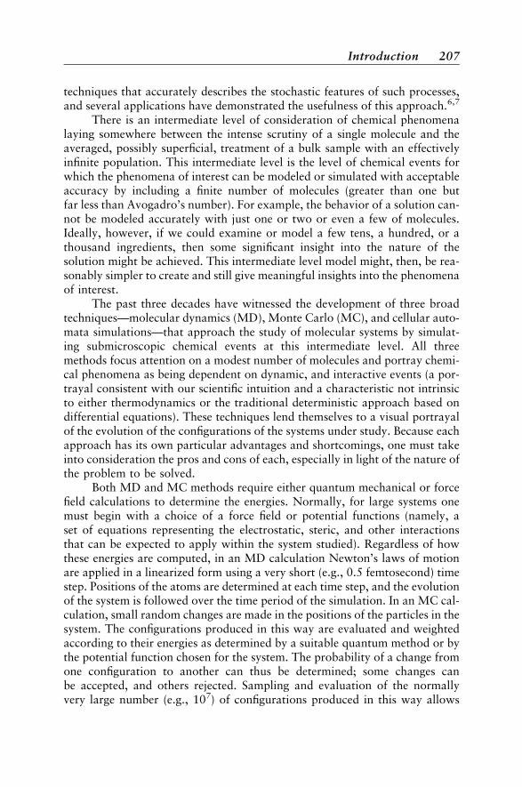
techniques that accurately describes the stochastic features of such processes,and several applications have demonstrated the usefulness of this approach.6,7

There is an intermediate level of consideration of chemical phenomenalaying somewhere between the intense scrutiny of a single molecule and theaveraged, possibly superficial, treatment of a bulk sample with an effectivelyinfinite population. This intermediate level is the level of chemical events forwhich the phenomena of interest can be modeled or simulated with acceptableaccuracy by including a finite number of molecules (greater than one butfar less than Avogadro’s number). For example, the behavior of a solution can-not be modeled accurately with just one or two or even a few of molecules.Ideally, however, if we could examine or model a few tens, a hundred, or athousand ingredients, then some significant insight into the nature of thesolution might be achieved. This intermediate level model might, then, be rea-sonably simpler to create and still give meaningful insights into the phenomenaof interest.

The past three decades have witnessed the development of three broadtechniques—molecular dynamics (MD), Monte Carlo (MC), and cellular auto-mata simulations—that approach the study of molecular systems by simulat-ing submicroscopic chemical events at this intermediate level. All threemethods focus attention on a modest number of molecules and portray chemi-cal phenomena as being dependent on dynamic, and interactive events (a por-trayal consistent with our scientific intuition and a characteristic not intrinsicto either thermodynamics or the traditional deterministic approach based ondifferential equations). These techniques lend themselves to a visual portrayalof the evolution of the configurations of the systems under study. Because eachapproach has its own particular advantages and shortcomings, one must takeinto consideration the pros and cons of each, especially in light of the nature ofthe problem to be solved.

Both MD and MC methods require either quantum mechanical or forcefield calculations to determine the energies. Normally, for large systems onemust begin with a choice of a force field or potential functions (namely, aset of equations representing the electrostatic, steric, and other interactionsthat can be expected to apply within the system studied). Regardless of howthese energies are computed, in an MD calculation Newton’s laws of motionare applied in a linearized form using a very short (e.g., 0.5 femtosecond) timestep. Positions of the atoms are determined at each time step, and the evolutionof the system is followed over the time period of the simulation. In an MC cal-culation, small random changes are made in the positions of the particles in thesystem. The configurations produced in this way are evaluated and weightedaccording to their energies as determined by a suitable quantum method or bythe potential function chosen for the system. The probability of a change fromone configuration to another can thus be determined; some changes canbe accepted, and others rejected. Sampling and evaluation of the normallyvery large number (e.g., 107) of configurations produced in this way allows

Introduction 207

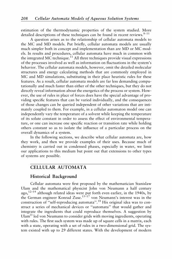
estimation of the thermodynamic properties of the system studied. Moredetailed descriptions of these techniques can be found in recent reviews.8–11

A question arises as to the relationship of cellular automata models tothe MC and MD models. Put briefly, cellular automata models are usuallymuch simpler both in concept and implementation than are MD or MC mod-els. In results and procedures, cellular automata have much in common withthe integrated MC technique.11 All three techniques provide visual expressionsof the processes involved as well as information on fluctuations in the system’sbehavior. The cellular automata models, however, omit the detailed molecularstructures and energy calculating methods that are commonly employed inMC and MD simulations, substituting in their place heuristic rules for thesefeatures. As a result, cellular automata models are far less demanding compu-tationally and much faster than either of the other techniques, but they do notdirectly reveal information about the energetics of the process or system. How-ever, the use of rules in place of forces does have the special advantage of pro-viding specific features that can be varied individually, and the consequencesof those changes can be queried independent of other variations that are inti-mately coupled to them. For example, in a cellular automaton model one canindependently vary the temperature of a solvent while keeping the temperatureof its solute constant in order to assess the effect of environmental tempera-ture, or one can increase one specific reaction or transition rate while holdingothers constant so as to isolate the influence of a particular process on theoverall dynamics of a system.

In the following sections, we describe what cellular automata are, howthey work, and then we provide examples of their uses. Because much ofchemistry is carried out in condensed phases, especially in water, we limitour applications to this medium but point out that extensions to other typesof systems are possible.

CELLULAR AUTOMATA

Historical Background

Cellular automata were first proposed by the mathematician StanislawUlam and the mathematical physicist John von Neumann a half centuryago,12–14 although related ideas were put forth even earlier, in the 1940s, bythe German engineer Konrad Zuse.15–17 von Neumann’s interest was in theconstruction of ‘‘self-reproducing automata’’.18 His original idea was to con-struct a series of mechanical devices or ‘‘automata’’ that would gather andintegrate the ingredients that could reproduce themselves. A suggestion byUlaml3 led von Neumann to consider grids with moving ingredients, operatingwith rules. The first such system was made up of square cells in a matrix, eachwith a state, operating with a set of rules in a two-dimensional grid. The sys-tem existed with up to 29 different states. With the development of modern

208 Cellular Automata Models of Aqueous Solution Systems

digital computers, it became increasingly clear that these fairly abstract ideascould in fact be usefully applied to the examination of real physical sys-tems.19,20 As described by Wolfram,21 cellular automata have five fundamen-tal defining characteristics:

They consist of a discrete lattice of cells.

They evolve in discrete time steps.

Each site takes on a finite number of possible values.

The value of each site evolves according to the same deterministic rules.

The rules for the evolution of a site depend only on a local neighborhoodof sites around it.

As we shall see, the fourth characteristic can be modified to include prob-abilistic rules as well as deterministic rules. An important feature sometimesobserved in the evolution of these computational systems was the developmentof unanticipated patterns of ordered dynamical behavior, or ‘‘emergent prop-erties’’. As Kauffman has expressed it,22 ‘‘Studies of large, randomlyassembled cellular automata . . . have now demonstrated that such systemscan spontaneously crystallize enormously ordered dynamical behavior. Thiscrystallization hints that hitherto unexpected principles of order may befound, [and] that the order observed may have significant explanatory importin [biology and physics].’’ This proposal has borne considerable fruit, not onlyin biology and physics, but also in chemistry. Readers are referred to reviewsfor applications in physics23–26 and biology;27 selected physical and chemicalapplications have been reviewed by Chopard and co-workers.28

The General Structure

The simulation of a dynamic system using cellular automata requires sev-eral parts that make up the process. The cell is the basic model of each ingre-dient, molecule, or whatever constitutes the system. These cells may haveseveral shapes as part of the matrix or grid of cells. The grid may have bound-aries or be part of a topological object that eliminates boundaries. The cellsmay have rules that apply to all of the edges, or there may be different rulesfor each edge. This latter plan may impart more detail to the model, as neededfor a more detailed study.

The CellsCellular automata have been designed for one (1D), two (2D), or three-

dimensional (3D) arrays. The most commonly used is the 2D grid. The cellsmay be triangles, squares, hexagons, or other shapes in the 2D grid. Thesquare cell has been the one most widely used over the past 40 years. Eachcell in the grid is endowed with a primary state, namely, whether it is emptyor occupied with a particle, object, molecule, or whatever the system requires

Cellular Automata 209

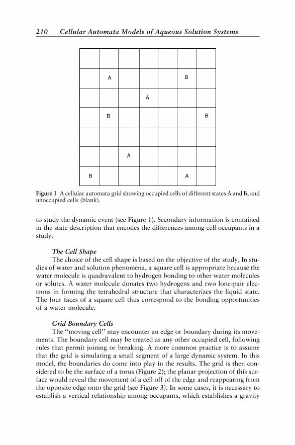
to study the dynamic event (see Figure 1). Secondary information is containedin the state description that encodes the differences among cell occupants in astudy.

The Cell ShapeThe choice of the cell shape is based on the objective of the study. In stu-

dies of water and solution phenomena, a square cell is appropriate because thewater molecule is quadravalent to hydrogen bonding to other water moleculesor solutes. A water molecule donates two hydrogens and two lone-pair elec-trons in forming the tetrahedral structure that characterizes the liquid state.The four faces of a square cell thus correspond to the bonding opportunitiesof a water molecule.

Grid Boundary CellsThe ‘‘moving cell’’ may encounter an edge or boundary during its move-

ments. The boundary cell may be treated as any other occupied cell, followingrules that permit joining or breaking. A more common practice is to assumethat the grid is simulating a small segment of a large dynamic system. In thismodel, the boundaries do come into play in the results. The grid is then con-sidered to be the surface of a torus (Figure 2); the planar projection of this sur-face would reveal the movement of a cell off of the edge and reappearing fromthe opposite edge onto the grid (see Figure 3). In some cases, it is necessary toestablish a vertical relationship among occupants, which establishes a gravity

B

B B

BA

A

A

A

Figure 1 A cellular automata grid showing occupied cells of different states A and B, andunoccupied cells (blank).

210 Cellular Automata Models of Aqueous Solution Systems

effect. In this situation, the grid is on the surface of a cylinder with a boundarycondition at the top and bottom, which is an impenetrable boundary.

Variegated Cell TypesUntil recently, all of the cellular automata models assumed that each

edge of a cell bore the same state and movement rules. Recent work has

Figure 2 The grid located on the surface of a torus. Column A of the grid is representedby line A on the torus; row B on the grid is represented by line B on the torus.

Figure 3 Movement of cell occu-pants at the boundaries of the gridon a torus. The cell occupant Amay move right and appear at theopposite side of the grid. Theother cell occupant A may movedown and appear at the top of thegrid.

Cellular Automata 211

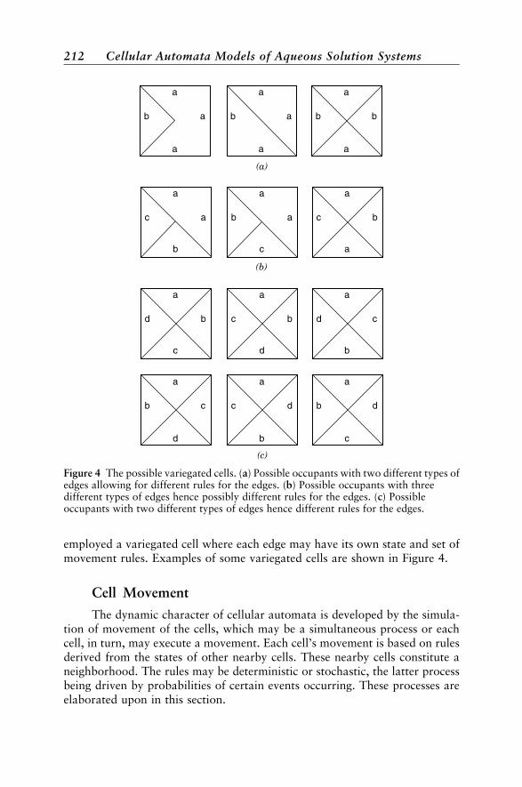
employed a variegated cell where each edge may have its own state and set ofmovement rules. Examples of some variegated cells are shown in Figure 4.

Cell Movement

The dynamic character of cellular automata is developed by the simula-tion of movement of the cells, which may be a simultaneous process or eachcell, in turn, may execute a movement. Each cell’s movement is based on rulesderived from the states of other nearby cells. These nearby cells constitute aneighborhood. The rules may be deterministic or stochastic, the latter processbeing driven by probabilities of certain events occurring. These processes areelaborated upon in this section.

b

a

a

a

b

a

a

a

b

a

b

a

(a)

c

b

a

a

b

c

a

a

c

a

b

a

(b)

d

c

b

a

c

d

b

a

d

b

c

a

b

d

c

a

c

b

d

a

b

c

d

a

(c)

Figure 4 The possible variegated cells. (a) Possible occupants with two different types ofedges allowing for different rules for the edges. (b) Possible occupants with threedifferent types of edges hence possibly different rules for the edges. (c) Possibleoccupants with two different types of edges hence different rules for the edges.

212 Cellular Automata Models of Aqueous Solution Systems

Synchronous–Asynchronous MovementWhen we speak of movement of a cell or the movement of cell occu-

pants, we are speaking of the simulation of a movement from one cell toanother. Thus a water molecule or some object is postulated to move acrossspace, appearing in a new location at time t þ 1. In the cellular automata mod-els, the actual situation is the exchange of state between two adjacent cells. Ifwe are modeling the movement of a molecule from place A to the adjacentplace B, then we must exchange the states of cells A and B. Initially, at timet, cell A has a state corresponding to an occupant molecule, while adjacent cellB is devoid of a molecule (i.e., it is empty). At time t þ 1, the states of the cellsA and B have exchanged. Cell A is empty, and cell B has the state of the occu-pant molecule. This exchange gives the illusion, and the practical conse-quences, of a movement from A to B. We speak of the movement of cells orof the movement of cell occupants; either way we are describing the process ofsimulating a movement as stated above.

Cell movement of all occupants in the grid may occur simultaneously(synchronous) or it may occur sequentially (asynchronous). When all cells inthe grid have computed their state and have executed their movement (or not)it is called one iteration, a unit of time in the cellular automata simulation.Each cell is identified in the program and is selected randomly for the choiceof movement or not. The question of which type of movement to use dependson the system being modeled and the information sought from the model, butit should reflect reality. If the system being studied is a slow process, then syn-chronous motion may best represent the process. In contrast, if the system isvery fast, like proton hopping among water molecules where the cellular au-tomata is using a few thousand cells, then an asynchronous model is desirable.A synchronous execution of the movement rules leads to possible competitionfor a cell from more than one occupant. A resolution scheme must thus be inplace to resolve the competition; otherwise this may interfere with the validityof the model.

NeighborhoodsCell movement is governed by rules called transition functions. The rules

involve the immediate environment of the cell called the neighborhood. Themost common neighborhood used in 2D cellular automata is called the vonNeumann neighborhood after the pioneer of the method. A cell, i, is in the cen-ter of four cells, j, adjoining the four faces of i, [see Figure 5(a) for this pat-tern]. Another common neighborhood is the Moore neighborhood [Figure5(b)], where cell i is completely surrounded by j cells. Other neighborhoodsinclude the extended von Neumann neighborhood shown in Figure 5(c), wherethe k cells beyond j are identified and allowed to participate in movements.

Deterministic/Probabilistic Movement RulesThe rules governing cell movement may be deterministic or probabilistic.

Deterministic cellular automata use a fixed set of rules, the values of which are

Cellular Automata 213

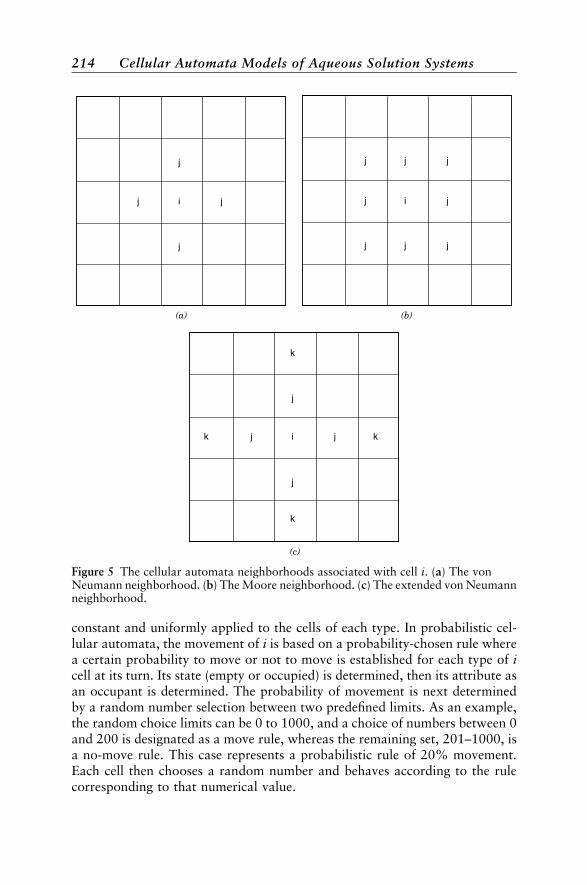
constant and uniformly applied to the cells of each type. In probabilistic cel-lular automata, the movement of i is based on a probability-chosen rule wherea certain probability to move or not to move is established for each type of icell at its turn. Its state (empty or occupied) is determined, then its attribute asan occupant is determined. The probability of movement is next determinedby a random number selection between two predefined limits. As an example,the random choice limits can be 0 to 1000, and a choice of numbers between 0and 200 is designated as a move rule, whereas the remaining set, 201–1000, isa no-move rule. This case represents a probabilistic rule of 20% movement.Each cell then chooses a random number and behaves according to the rulecorresponding to that numerical value.

j j

j

j

i

(a)

j

j

j

j

j

jj

j

i

(b)

j j

j

j

k

k

kk i

(c)

Figure 5 The cellular automata neighborhoods associated with cell i. (a) The vonNeumann neighborhood. (b) The Moore neighborhood. (c) The extended von Neumannneighborhood.

214 Cellular Automata Models of Aqueous Solution Systems

Movement (Transition) Rules

The movement of cells is based upon rules governing the events inherentin cellular automata dynamics. The rules describe the probabilities of twoadjacent cells separating, two cells joining at a face, two cells displacing eachother in a gravity simulation, or a cell with different designated edges rotatingin the grid. These events are the essence of the cellular automata dynamics andproduce configurations that may possibly mirror physical events. The follow-ing sections develop these topics, and the Appendix provides technical detailabout the hardware and software used and defines the directional movingprobability, MP(d), for each direction d.

General Conditions for Water ModelsSeveral probabilistic rules are used to govern the trajectories of molecules

moving in the grid. The first set of these rules, called transition functions, gov-ern the movement of the occupied cells across the grid. The rules respond tothe immediate neighborhood of the occupied cell, thus all events are local. Aprobabilistic or stochastic set of rules operating in a grid on the surface of atorus is most appropriate for the simulation of water and solution phenomena.This arrangement provides a near-infinitely large system with no boundaryconditions.

The Free Movement ProbabilityThe first rule is the movement probability Pm. This rule involves the

probability that an occupant in an unbound cell, i, will move to one of fouradjacent cells, j, if that space is unoccupied. An example is cell i in Figure 6that may move (in its turn) to any unoccupied cell, j. If it moves to a cell whoseneighbor is an occupied cell, k, then a bond will form between cells i and k. As

j j k

k

k

k

j

j

i

Figure 6 Possible movement of cell ioccupant to unoccupied cell j.

Cellular Automata 215

a matter of course, this probability, Pm, is usually set at 1.0, which means thatthis event always happens (a rule).

Breaking RulesJust as two cells can join together, so their tessellated state can be bro-

ken. The first of two trajectory or interaction rules is the breaking probabilityPB. To comprehend this, it is convenient to refer to the occupant of a cell as amolecule. The PB(AB) rule is the probability for a molecule A, bonded to mole-cule B, to break away from B, as shown in Figure 7(a). The value for PB liesbetween 0 and 1. If molecule A is bonded to two molecules, B and B, the simul-taneous probability of a breaking away event from both B and B isPB(AB)*PB(AB), as shown in Figure 7(b). If molecule A is bound to three othermolecules, B, B, and B, the simultaneous breaking probability of molecule A isPB(AB)*PB(AB)*(PB(AB), shown in Figure 7(c). If molecule A is surrounded byfour molecules, it cannot move on this 2D grid.

Joining ParameterA joining trajectory parameter, J(AB), describes the movement of a mole-

cule at A to join with a molecule at B, when an intermediate cell is vacant(see Figure 8). This rule follows the rule to move or not to move describedabove. The parameter J is a nonnegative real number. When J ¼ 1, moleculeA has the same probability of movement toward or away from B as for thecase when the B cell is empty. When J>1, molecule A has a greater probabilityof movement toward an occupied cell B than when cell B is empty. When0< J<1, molecule A has a lower probability of such movement. WhenJ ¼ 0, molecule A cannot make any movement.

Relative GravityThe simulation of a ‘‘gravity’’ effect has been introduced into the cellular

automata paradigm to model separating phenomena such as the demixing ofimmiscible liquids or the flow of solutions in a chromatographic separation.To accomplish this effect, a boundary condition is imposed at the upper andlower edges of the grid to simulate a vertical versus a horizontal relationship.The differential effect of gravity is simulated by introducing two new rulesgoverning the preferences of two cells of different composition to exchangepositions when they are in a vertically joined state. When molecule A is ontop of a second molecule B, then two new rules are actuated. The first rule,GD(AB), is the probability that molecule A will exchange places withmolecule B, assuming a position below B. The other gravity term is GD(BA),which expresses the probability that molecule B will occupy a position beneathmolecule A. These rules are illustrated in Figure 9. In the absence of any strongevidence to support the model that the two gravity rules are complementary toeach other in general, the treatment described above reflects the situation inwhich the gravity effects of A and B are two separate random events. Based

216 Cellular Automata Models of Aqueous Solution Systems

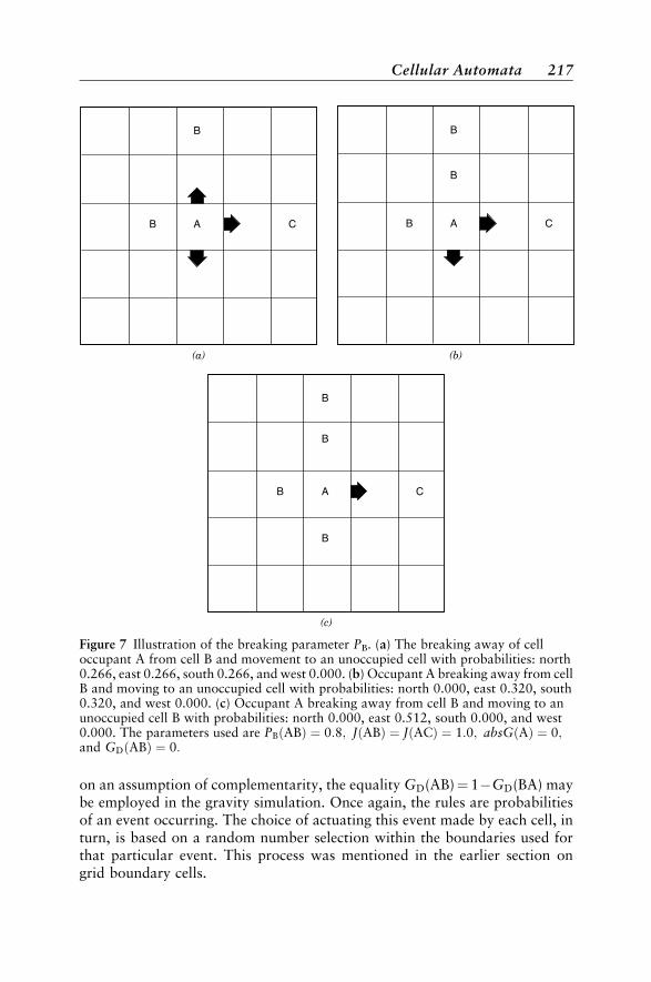
on an assumption of complementarity, the equality GD(AB)¼ 1GD(BA) maybe employed in the gravity simulation. Once again, the rules are probabilitiesof an event occurring. The choice of actuating this event made by each cell, inturn, is based on a random number selection within the boundaries used forthat particular event. This process was mentioned in the earlier section ongrid boundary cells.

B C

B

A

(a)

B C

B

B

A

(b)

B C

B

B

B

A

(c)

Figure 7 Illustration of the breaking parameter PB. (a) The breaking away of celloccupant A from cell B and movement to an unoccupied cell with probabilities: north0.266, east 0.266, south 0.266, and west 0.000. (b) Occupant A breaking away from cellB and moving to an unoccupied cell with probabilities: north 0.000, east 0.320, south0.320, and west 0.000. (c) Occupant A breaking away from cell B and moving to anunoccupied cell B with probabilities: north 0.000, east 0.512, south 0.000, and west0.000. The parameters used are PBðABÞ ¼ 0:8; JðABÞ ¼ JðACÞ ¼ 1:0; absGðAÞ ¼ 0;and GDðABÞ ¼ 0:

Cellular Automata 217

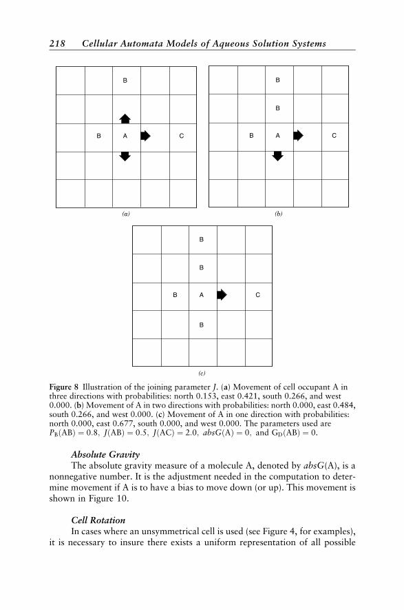
Absolute GravityThe absolute gravity measure of a molecule A, denoted by absG(A), is a

nonnegative number. It is the adjustment needed in the computation to deter-mine movement if A is to have a bias to move down (or up). This movement isshown in Figure 10.

Cell RotationIn cases where an unsymmetrical cell is used (see Figure 4, for examples),

it is necessary to insure there exists a uniform representation of all possible

B C

B

A

(a)

B C

B

B

A

(b)

B C

B

B

B

A

(c)

Figure 8 Illustration of the joining parameter J. (a) Movement of cell occupant A inthree directions with probabilities: north 0.153, east 0.421, south 0.266, and west0.000. (b) Movement of A in two directions with probabilities: north 0.000, east 0.484,south 0.266, and west 0.000. (c) Movement of A in one direction with probabilities:north 0.000, east 0.677, south 0.000, and west 0.000. The parameters used arePBðABÞ ¼ 0:8; JðABÞ ¼ 0:5; JðACÞ ¼ 2:0; absGðAÞ ¼ 0; and GDðABÞ ¼ 0.

218 Cellular Automata Models of Aqueous Solution Systems

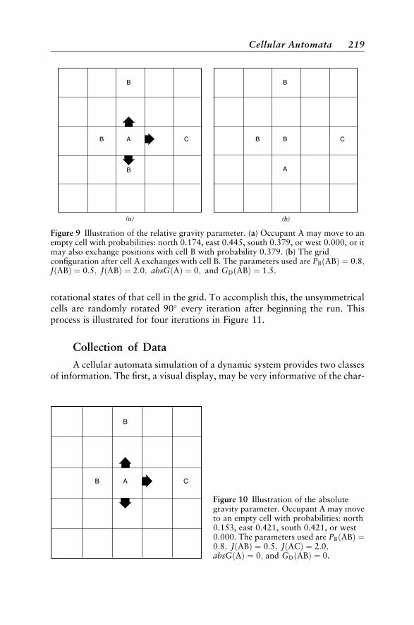
rotational states of that cell in the grid. To accomplish this, the unsymmetricalcells are randomly rotated 90 every iteration after beginning the run. Thisprocess is illustrated for four iterations in Figure 11.

Collection of Data

A cellular automata simulation of a dynamic system provides two classesof information. The first, a visual display, may be very informative of the char-

B C

B

B

A

(a)

B B C

B

A

(b)

Figure 9 Illustration of the relative gravity parameter. (a) Occupant A may move to anempty cell with probabilities: north 0.174, east 0.445, south 0.379, or west 0.000, or itmay also exchange positions with cell B with probability 0.379. (b) The gridconfiguration after cell A exchanges with cell B. The parameters used are PBðABÞ ¼ 0:8;JðABÞ ¼ 0:5; JðABÞ ¼ 2:0; absGðAÞ ¼ 0; and GDðABÞ ¼ 1:5.

B C

B

A

Figure 10 Illustration of the absolutegravity parameter. Occupant A may moveto an empty cell with probabilities: north0.153, east 0.421, south 0.421, or west0.000. The parameters used are PBðABÞ ¼0:8; JðABÞ ¼ 0:5; JðACÞ ¼ 2:0;absGðAÞ ¼ 0; and GDðABÞ ¼ 0.

Cellular Automata 219

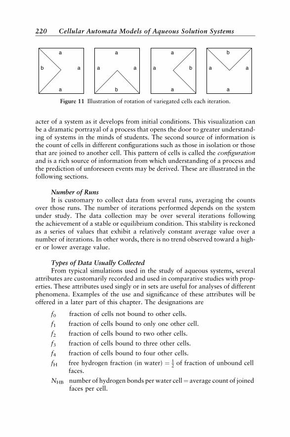
acter of a system as it develops from initial conditions. This visualization canbe a dramatic portrayal of a process that opens the door to greater understand-ing of systems in the minds of students. The second source of information isthe count of cells in different configurations such as those in isolation or thosethat are joined to another cell. This pattern of cells is called the configurationand is a rich source of information from which understanding of a process andthe prediction of unforeseen events may be derived. These are illustrated in thefollowing sections.

Number of RunsIt is customary to collect data from several runs, averaging the counts

over those runs. The number of iterations performed depends on the systemunder study. The data collection may be over several iterations followingthe achievement of a stable or equilibrium condition. This stability is reckonedas a series of values that exhibit a relatively constant average value over anumber of iterations. In other words, there is no trend observed toward a high-er or lower average value.

Types of Data Usually CollectedFrom typical simulations used in the study of aqueous systems, several

attributes are customarily recorded and used in comparative studies with prop-erties. These attributes used singly or in sets are useful for analyses of differentphenomena. Examples of the use and significance of these attributes will beoffered in a later part of this chapter. The designations are

f0 fraction of cells not bound to other cells.

f1 fraction of cells bound to only one other cell.

f2 fraction of cells bound to two other cells.

f3 fraction of cells bound to three other cells.

f4 fraction of cells bound to four other cells.

fH free hydrogen fraction (in water) ¼ 12 of fraction of unbound cell

faces.

NHB number of hydrogen bonds per water cell¼ average count of joinedfaces per cell.

a

a

ab a

a

a

b

a

a

a

b a a

a

b

Figure 11 Illustration of rotation of variegated cells each iteration.

220 Cellular Automata Models of Aqueous Solution Systems

In addition, the average distance that a cell travels may be another datumcollected.

AQUEOUS SOLUTION SYSTEMS

Water as a System

It has long been recognized that water plays an essential part in chemicalevents especially those associated with drug phenomena including drug–recep-tor encounters. Water is viewed as an active participant in the complex systemcomposed of drug–receptor–water. Along with these encounters, there are ahost of pharmacodynamic events occurring in aqueous solution includingdrug absorption, distribution, metabolism, and elimination (ADME). It isessential then to add to the understanding of this essential fluid and the com-plex systems it forms when solutes enter its embrace.

When solution ingredients interact, there emerges in the system a set ofproperties not clearly recognizable as additive contributions from the ingredi-ents. There is formed a complex system characterized by new properties. Thesubjects of complexity and emergent properties in drug research have beenreviewed by Kier and Testa.29 The complex nature of water and solutions isrecognized and has prompted some investigators to derive models based onnonlinear combinations of ingredients. In particular, we have witnessed thegrowth of MC and MD simulations of water that have added to our under-standing of its complex character.30–34 However, the large amount of compu-ter time required by MD and MC coupled with assumptions of specific forcefields produces certain limitations. An alternative to these two simulationmethods that reduces some of these problems is the cellular automata modelof dynamic synthesis.

A prominent model of water is that of an extended network of hydrogen-bonded molecules that lack a single, identifiable, long-lived structure.35 Thehydrogen bonds continually form and break producing a constantly changingmosaic when viewed at the molecular system level. This model lends itself tosimulation using dynamic methods such as cellular automata. Kier andCheng36 created such a model of liquid water using rules governing the joiningand breaking of water-designated cells. This model provided the computa-tional basis for further studies of aqueous solution phenomena, described inthis part of the chapter.

The Molecular Model

We want to make clear just what the cells, the configurations generated,and the cellular automata models represent. This effort will help with under-standing the results of a simulation and limiting misunderstanding based on

Aqueous Solution Systems 221

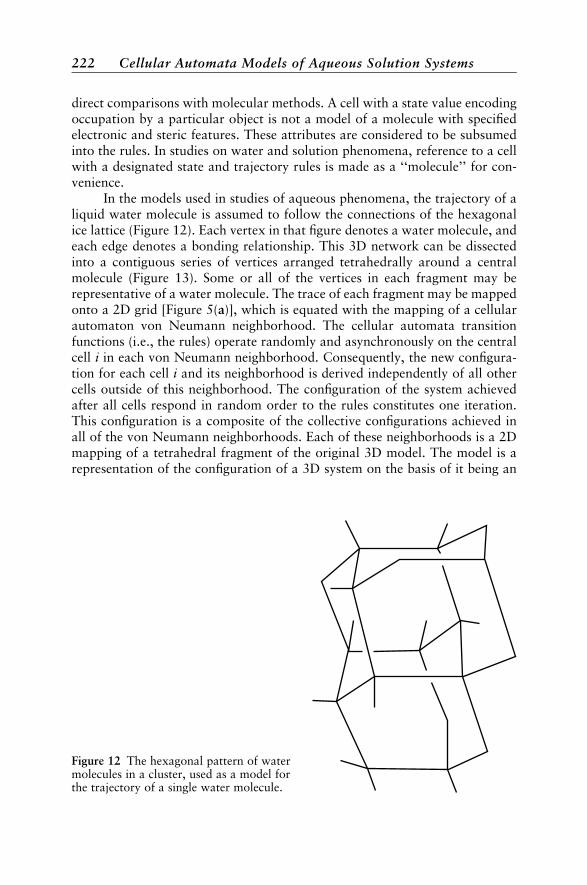
direct comparisons with molecular methods. A cell with a state value encodingoccupation by a particular object is not a model of a molecule with specifiedelectronic and steric features. These attributes are considered to be subsumedinto the rules. In studies on water and solution phenomena, reference to a cellwith a designated state and trajectory rules is made as a ‘‘molecule’’ for con-venience.

In the models used in studies of aqueous phenomena, the trajectory of aliquid water molecule is assumed to follow the connections of the hexagonalice lattice (Figure 12). Each vertex in that figure denotes a water molecule, andeach edge denotes a bonding relationship. This 3D network can be dissectedinto a contiguous series of vertices arranged tetrahedrally around a centralmolecule (Figure 13). Some or all of the vertices in each fragment may berepresentative of a water molecule. The trace of each fragment may be mappedonto a 2D grid [Figure 5(a)], which is equated with the mapping of a cellularautomaton von Neumann neighborhood. The cellular automata transitionfunctions (i.e., the rules) operate randomly and asynchronously on the centralcell i in each von Neumann neighborhood. Consequently, the new configura-tion for each cell i and its neighborhood is derived independently of all othercells outside of this neighborhood. The configuration of the system achievedafter all cells respond in random order to the rules constitutes one iteration.This configuration is a composite of the collective configurations achieved inall of the von Neumann neighborhoods. Each of these neighborhoods is a 2Dmapping of a tetrahedral fragment of the original 3D model. The model is arepresentation of the configuration of a 3D system on the basis of it being an

Figure 12 The hexagonal pattern of watermolecules in a cluster, used as a model forthe trajectory of a single water molecule.

222 Cellular Automata Models of Aqueous Solution Systems

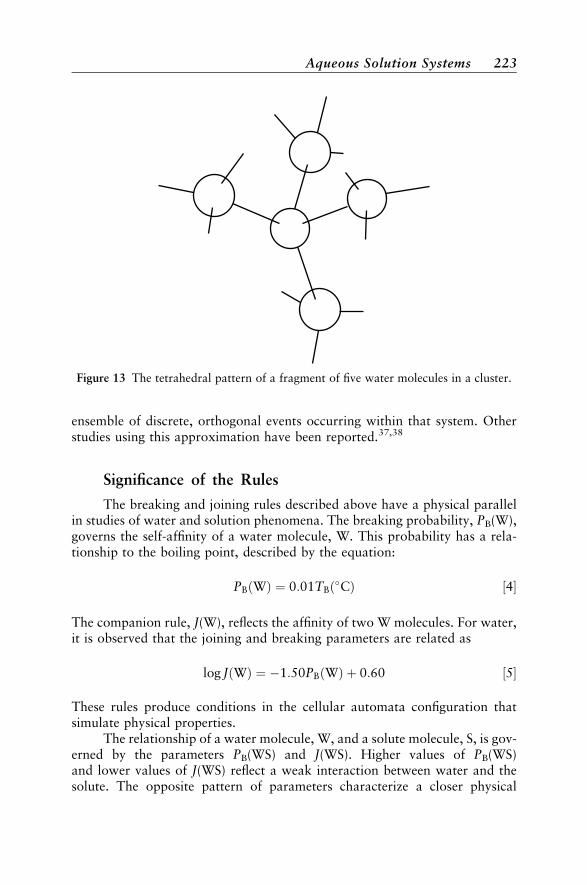
ensemble of discrete, orthogonal events occurring within that system. Otherstudies using this approximation have been reported.37,38

Significance of the Rules

The breaking and joining rules described above have a physical parallelin studies of water and solution phenomena. The breaking probability, PB(W),governs the self-affinity of a water molecule, W. This probability has a rela-tionship to the boiling point, described by the equation:

PBðWÞ ¼ 0:01TBðCÞ ½4

The companion rule, J(W), reflects the affinity of two W molecules. For water,it is observed that the joining and breaking parameters are related as

log JðWÞ ¼ 1:50PBðWÞ þ 0:60 ½5

These rules produce conditions in the cellular automata configuration thatsimulate physical properties.

The relationship of a water molecule, W, and a solute molecule, S, is gov-erned by the parameters PB(WS) and J(WS). Higher values of PB(WS)and lower values of J(WS) reflect a weak interaction between water and thesolute. The opposite pattern of parameters characterize a closer physical

Figure 13 The tetrahedral pattern of a fragment of five water molecules in a cluster.

Aqueous Solution Systems 223

relationship between water and solute. These patterns ultimately translate intosimulations of solubility, the hydrophobic effect, and diffusion preferences.

STUDIES OF WATER AND SOLUTION PHENOMENA

A Cellular Automata Model of Water

In a study of water, Kier and Cheng36 found relationships between theaverage cluster size and viscosity, and between the fraction of unbound cells,f0, and the vapor pressure. The number of water-designated cells was chosento be 69% of the cells in the grid, this value giving a concentration of unboundwater molecules in agreement with earlier predictions and experiments.30,39

More recent studies have examined all the fx attributes from the rules PB

and J, whereby the PB(W) value was systematically varied. A profile of watercells, described by the fraction of each bonding type, f0–f4, for each ‘‘tempera-ture’’, is shown in Figure 14. The values of f0 correspond closely to the valuesused by Walrafen39 and Haggis et al.40 to predict the dielectric constant andheat capacity of water. This finding led to the conjecture that the rules chosengive rise to configurations mirroring physical reality. A test of this possibility isreported in Table 1 where a set of equations relating several physical proper-ties of water to attributes from the cellular automata simulations are shown. Inaddition to the examples in the table, the free hydrogen fraction, fH, is close tothe value of about 15% reported from infrared (IR) evidence of the free OHcontent.41 These correlations between simulated water attributes and variousphysical properties suggest that the water model created with cellular auto-mata has validity.36

The Hydrophobic Effect

The hydrophobic effect is a term describing the influence of relativelynonpolar (lipophilic) substances on the collective behavior of water moleculesin their vicinity. The common expression is that water is ‘‘more structured’’ ororganized when in contact with a lipophilic solute. This behavior was observedin a cellular automata model of a solute in water,42,43 which led to a study inmore detail.44 The hydrophobic effect was modeled by systematically increas-ing the breaking probability, PB(WS), value, encoding an increasing probabil-ity of a solute molecule, S, not to associate with water.

It was observed that low PB(WS) values, modeling a polar molecule,produced configurations in which the solute molecules were extensively sur-rounded by water molecules, a pattern simulating hydration or electrostric-tion. Conversely, with high values of PB(WS) most of the solute moleculeswere found outside of the water clusters and within the cavities. This config-uration leaves the water clusters relatively free of solute; hence they are more

224 Cellular Automata Models of Aqueous Solution Systems

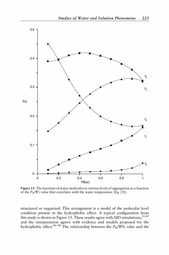
structured or organized. This arrangement is a model of the molecular levelcondition present in the hydrophobic effect. A typical configuration fromthis study is shown in Figure 15. These results agree with MD simulations,31,45

and the interpretation agrees with evidence and models proposed for thehydrophobic effect.46–48 The relationship between the PB(WS) rules and the

0

0

0.2

0.1

0.2

0.3

0.4

0.5

0.4PB(w)

0.6 0.8 1

f(x)

f0

f1

f4

f2

f3

Figure 14 The fractions of water molecules in various levels of aggregation as a functionof the PB(W) value that correlates with the water temperature (Eq. [5]).

Studies of Water and Solution Phenomena 225

relative lipophilicity of a solute molecule is a useful rule for further studies onsolution phenomena.

Solute Dissolution

Cellular automata simulations of the dissolution process have beendescribed.42 The solute molecules, S, started in a solid block of cells at the cen-ter of the grid. They are endowed with rules PB(S), J(S), PB(WS), and J(WS).The attributes recorded from the dynamics were the f0(S), fraction of solutesunbound to other solute molecules, plus the average number of solute–solutejoined faces, T(S), and the average distance that solute molecules have traveledfrom the center of the block at some specific iteration, D(S). The f0(S) valueswere interpreted to represent the extent of dissolution of the solute. Thedecrease in the T(S) values characterize the extent of disruption of the soluteblock, whereas the D(S) values quantify the extent of diffusion of solutes intothe surrounding water.

The effects of the four joining and breaking parameters, PB(WS), J(WS),PB(S), and J(S), were studied using a high and a low numerical value for each.From the results several conclusions were drawn about the influence of therules and about some aspects of the process. The extent and rate of the solutecluster disruption, which is reflected by T(S), is primarily a function of thePB(S) rule with secondary influence from the PB(WS) rule. A high value ofPB(S) is a rule governing a high probability of solute molecules separatingfrom each other; hence the rule may be viewed as the effective melting processrelating to crystal disruption. The dissolved state was considered to exist whenan isolated solute cell is present. The f0 fraction is a measure of the extent ofthe modeled solubility. The extent of dissolution depends on both the PB(S)and the PB(WS) rules. High values of PB(S) and low values of PB(WS) promotean extensive degree of dissolution. A low value of PB(WS) characterizes asolute that is relatively polar and hydrophilic. The studies also showed thatsolutes with high PB(WS) values diffuse more rapidly than those with lowvalues. The interpretation is that the more lipophilic the solute molecule, thegreater its diffusion rate. It was also observed that simulations of highertemperatures led to faster disruption of the block of solute, more f0 molecular

Table 1 Water Properties Related to Cellular Automata Attributes

Property Equation r2 Correlation

Vapor pressure log Pvðmm HgÞ ¼ 13:77ð f0 þ f1Þ þ 0:795 0.987Dielectric constant e ¼ 224f1 þ 86:9 0.989Viscosity ZðcentipoiseÞ ¼ 3:165f4 0:187 0.989Ionization logKw ¼ 20:94fH þ 16:43 0.999Surface tension gðdyn=cmÞ ¼ 16:07NHB þ 22:35 0.970Compressibility kð106=barÞ ¼ 53:82 f3 þ 66:66 0.953

226 Cellular Automata Models of Aqueous Solution Systems

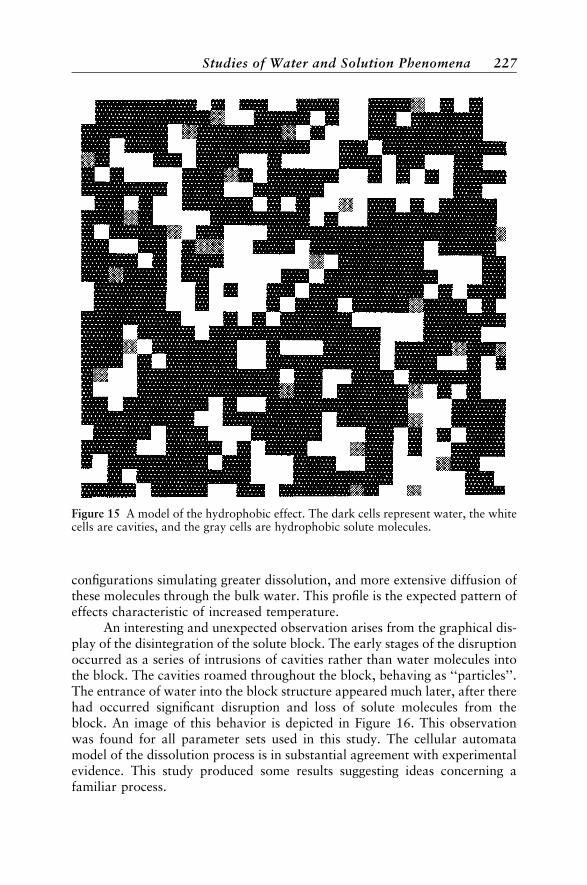
configurations simulating greater dissolution, and more extensive diffusion ofthese molecules through the bulk water. This profile is the expected pattern ofeffects characteristic of increased temperature.

An interesting and unexpected observation arises from the graphical dis-play of the disintegration of the solute block. The early stages of the disruptionoccurred as a series of intrusions of cavities rather than water molecules intothe block. The cavities roamed throughout the block, behaving as ‘‘particles’’.The entrance of water into the block structure appeared much later, after therehad occurred significant disruption and loss of solute molecules from theblock. An image of this behavior is depicted in Figure 16. This observationwas found for all parameter sets used in this study. The cellular automatamodel of the dissolution process is in substantial agreement with experimentalevidence. This study produced some results suggesting ideas concerning afamiliar process.

Figure 15 A model of the hydrophobic effect. The dark cells represent water, the whitecells are cavities, and the gray cells are hydrophobic solute molecules.

Studies of Water and Solution Phenomena 227

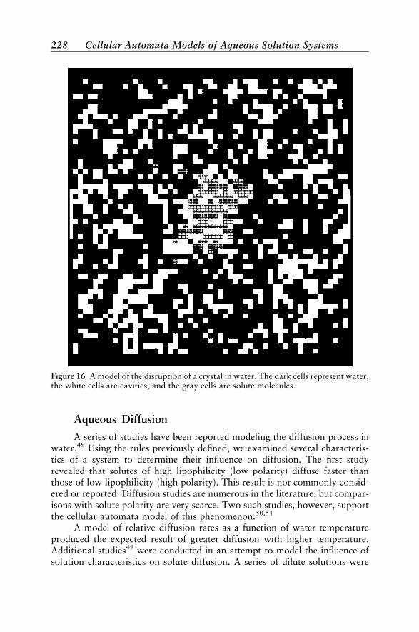
Aqueous Diffusion

A series of studies have been reported modeling the diffusion process inwater.49 Using the rules previously defined, we examined several characteris-tics of a system to determine their influence on diffusion. The first studyrevealed that solutes of high lipophilicity (low polarity) diffuse faster thanthose of low lipophilicity (high polarity). This result is not commonly consid-ered or reported. Diffusion studies are numerous in the literature, but compar-isons with solute polarity are very scarce. Two such studies, however, supportthe cellular automata model of this phenomenon.50,51

A model of relative diffusion rates as a function of water temperatureproduced the expected result of greater diffusion with higher temperature.Additional studies49 were conducted in an attempt to model the influence ofsolution characteristics on solute diffusion. A series of dilute solutions were

Figure 16 A model of the disruption of a crystal in water. The dark cells represent water,the white cells are cavities, and the gray cells are solute molecules.

228 Cellular Automata Models of Aqueous Solution Systems

modeled whereby the relative lipophilicity of a solute S1 was varied. A secondsolute, S2, was introduced at the center of the grid. The dynamics showed thatthe solute S2 diffused faster when there is no cosolute and when the polarity ofS2 is low. The presence of the cosolute revealed that the diffusion of S2 wasfastest when the cosolvent S1 was lipophilic.

In another study,49 the grid was divided into two halves, the upper half,containing a solution of a relatively nonpolar solute, while the lower half con-tained a solution of a relatively polar solute. Between these two halves, a thinlayer of cells simulated a solution made up of a solute of intermediate polarity.The dynamics created a model in which the solute in the middle layer prefer-entially diffused into the upper layer containing the nonpolar solute. A secondstudy simulated an aqueous solution of intermediate polarity in the middle ofthe grid. Surrounding this solution were regions with highly polar, intermedi-ately polar, and nonpolar solutes in solution. A fourth region around the cen-ter was pure water. The solute in the central section of the grid was allowed todiffuse freely. It diffused more rapidly into the pure water; however, it second-arily preferred the more nonpolar solution quadrant. This finding is consistentwith the results from the studies described above. The diffusion of a solute ismodeled to be faster when it is lipophilic and when cosolutes are lipophilic.

Immiscible Liquids and Partitioning

Cheng and Kier modeled the separation of immiscible liquids and thepartitioning of a solute between them.52,53 For this study, the cellular automa-ta grid had to be modified to create a model of the differential effect on theingredients due to ‘‘gravity’’. To accomplish this, boundary conditions wereimposed at the upper and lower edges of the grid to contain the liquids in aclosed system. The differential effect of gravity was modeled by introducingthe rules described earlier.

The water cells were ruled to have high self-affinities and low affinitieswith the other solvent. A PB(WS1) rule was chosen with a high value to endowthe two liquids with markedly different polarities. The emerging configurationcan thus be described as being an immiscible, two-phase system. Each experi-ment began with a random distribution of equal numbers of water and S1 cells,the sum totaling 69% of the grid space. The breaking and joining parameterswere chosen to create significant self-affinity between each type of ingredientand a weak affinity between different types. The gravity terms were chosen tofavor the water cell moving to the lower position relative to the other solvent.

At a very early iteration time, there formed small, vertically orientedstacks of water cells in the upper half of the grid and similar stacks of S1 inthe lower half of the grid. These stacks steadily enlarged and moved towardthe central part of the grid. Aggregation of each common type of cell stackoccurred as they moved toward the central section of the grid. An interfaceformed with a greater concentration of water in the lower half while the

Studies of Water and Solution Phenomena 229

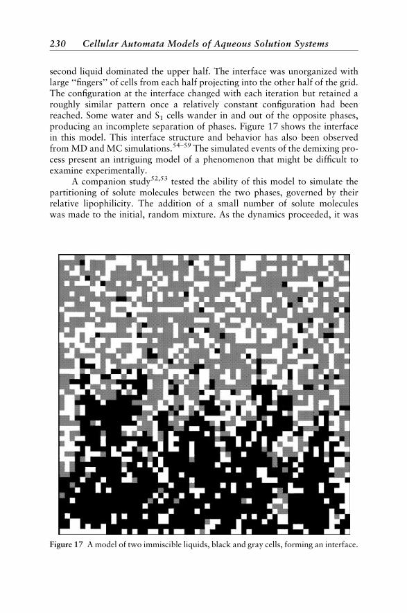
second liquid dominated the upper half. The interface was unorganized withlarge ‘‘fingers’’ of cells from each half projecting into the other half of the grid.The configuration at the interface changed with each iteration but retained aroughly similar pattern once a relatively constant configuration had beenreached. Some water and S1 cells wander in and out of the opposite phases,producing an incomplete separation of phases. Figure 17 shows the interfacein this model. This interface structure and behavior has also been observedfrom MD and MC simulations.54–59 The simulated events of the demixing pro-cess present an intriguing model of a phenomenon that might be difficult toexamine experimentally.

A companion study52,53 tested the ability of this model to simulate thepartitioning of solute molecules between the two phases, governed by theirrelative lipophilicity. The addition of a small number of solute moleculeswas made to the initial, random mixture. As the dynamics proceeded, it was

Figure 17 A model of two immiscible liquids, black and gray cells, forming an interface.

230 Cellular Automata Models of Aqueous Solution Systems

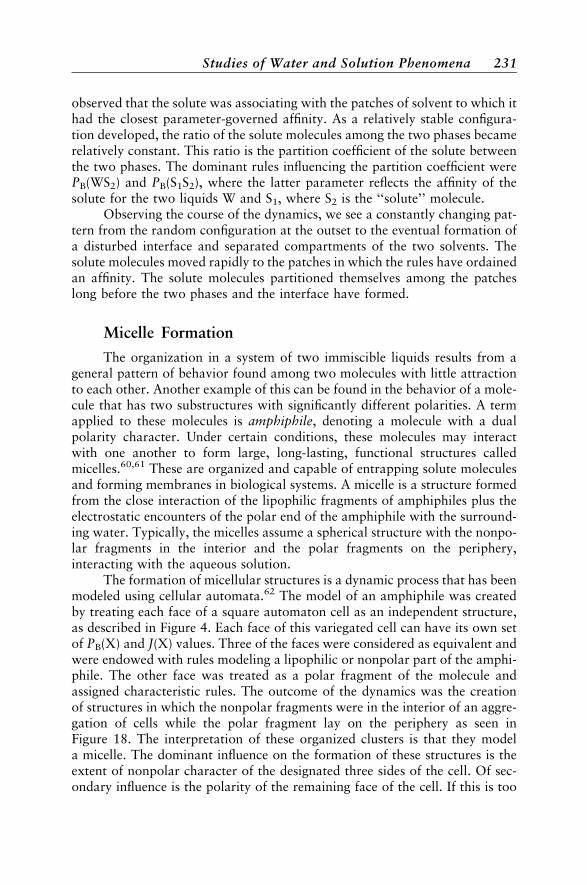
observed that the solute was associating with the patches of solvent to which ithad the closest parameter-governed affinity. As a relatively stable configura-tion developed, the ratio of the solute molecules among the two phases becamerelatively constant. This ratio is the partition coefficient of the solute betweenthe two phases. The dominant rules influencing the partition coefficient werePB(WS2) and PB(S1S2), where the latter parameter reflects the affinity of thesolute for the two liquids W and S1, where S2 is the ‘‘solute’’ molecule.

Observing the course of the dynamics, we see a constantly changing pat-tern from the random configuration at the outset to the eventual formation ofa disturbed interface and separated compartments of the two solvents. Thesolute molecules moved rapidly to the patches in which the rules have ordainedan affinity. The solute molecules partitioned themselves among the patcheslong before the two phases and the interface have formed.

Micelle Formation

The organization in a system of two immiscible liquids results from ageneral pattern of behavior found among two molecules with little attractionto each other. Another example of this can be found in the behavior of a mole-cule that has two substructures with significantly different polarities. A termapplied to these molecules is amphiphile, denoting a molecule with a dualpolarity character. Under certain conditions, these molecules may interactwith one another to form large, long-lasting, functional structures calledmicelles.60,61 These are organized and capable of entrapping solute moleculesand forming membranes in biological systems. A micelle is a structure formedfrom the close interaction of the lipophilic fragments of amphiphiles plus theelectrostatic encounters of the polar end of the amphiphile with the surround-ing water. Typically, the micelles assume a spherical structure with the nonpo-lar fragments in the interior and the polar fragments on the periphery,interacting with the aqueous solution.

The formation of micellular structures is a dynamic process that has beenmodeled using cellular automata.62 The model of an amphiphile was createdby treating each face of a square automaton cell as an independent structure,as described in Figure 4. Each face of this variegated cell can have its own setof PB(X) and J(X) values. Three of the faces were considered as equivalent andwere endowed with rules modeling a lipophilic or nonpolar part of the amphi-phile. The other face was treated as a polar fragment of the molecule andassigned characteristic rules. The outcome of the dynamics was the creationof structures in which the nonpolar fragments were in the interior of an aggre-gation of cells while the polar fragment lay on the periphery as seen inFigure 18. The interpretation of these organized clusters is that they modela micelle. The dominant influence on the formation of these structures is theextent of nonpolar character of the designated three sides of the cell. Of sec-ondary influence is the polarity of the remaining face of the cell. If this is too

Studies of Water and Solution Phenomena 231

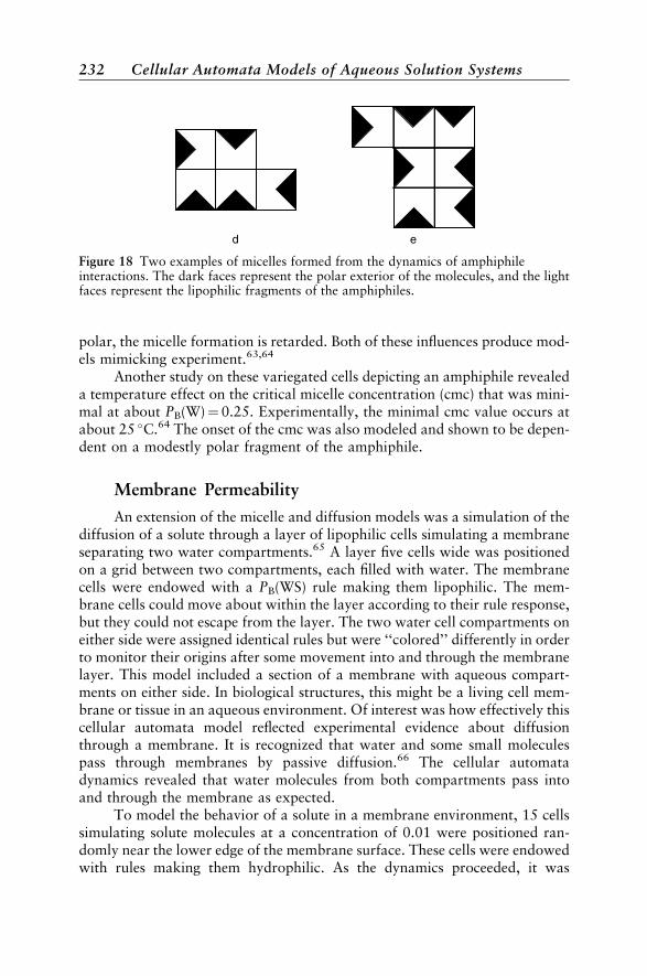
polar, the micelle formation is retarded. Both of these influences produce mod-els mimicking experiment.63,64

Another study on these variegated cells depicting an amphiphile revealeda temperature effect on the critical micelle concentration (cmc) that was mini-mal at about PB(W)¼ 0.25. Experimentally, the minimal cmc value occurs atabout 25 C.64 The onset of the cmc was also modeled and shown to be depen-dent on a modestly polar fragment of the amphiphile.

Membrane Permeability

An extension of the micelle and diffusion models was a simulation of thediffusion of a solute through a layer of lipophilic cells simulating a membraneseparating two water compartments.65 A layer five cells wide was positionedon a grid between two compartments, each filled with water. The membranecells were endowed with a PB(WS) rule making them lipophilic. The mem-brane cells could move about within the layer according to their rule response,but they could not escape from the layer. The two water cell compartments oneither side were assigned identical rules but were ‘‘colored’’ differently in orderto monitor their origins after some movement into and through the membranelayer. This model included a section of a membrane with aqueous compart-ments on either side. In biological structures, this might be a living cell mem-brane or tissue in an aqueous environment. Of interest was how effectively thiscellular automata model reflected experimental evidence about diffusionthrough a membrane. It is recognized that water and some small moleculespass through membranes by passive diffusion.66 The cellular automatadynamics revealed that water molecules from both compartments pass intoand through the membrane as expected.

To model the behavior of a solute in a membrane environment, 15 cellssimulating solute molecules at a concentration of 0.01 were positioned ran-domly near the lower edge of the membrane surface. These cells were endowedwith rules making them hydrophilic. As the dynamics proceeded, it was

d e

Figure 18 Two examples of micelles formed from the dynamics of amphiphileinteractions. The dark faces represent the polar exterior of the molecules, and the lightfaces represent the lipophilic fragments of the amphiphiles.

232 Cellular Automata Models of Aqueous Solution Systems

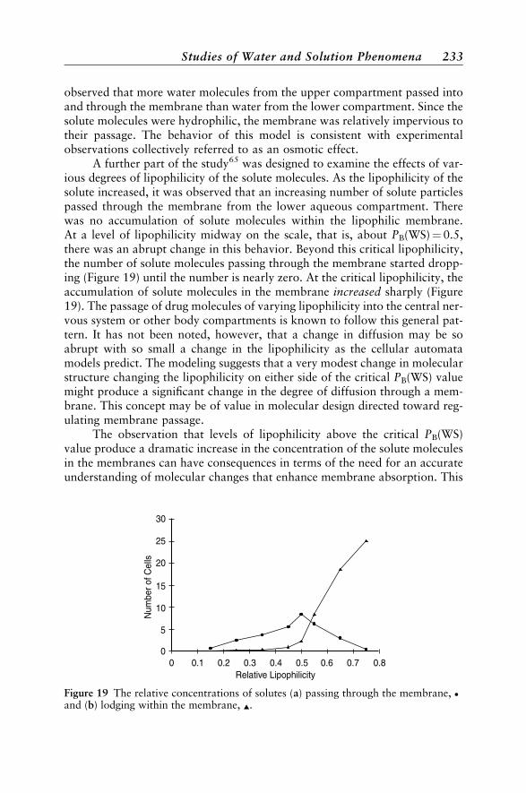
observed that more water molecules from the upper compartment passed intoand through the membrane than water from the lower compartment. Since thesolute molecules were hydrophilic, the membrane was relatively impervious totheir passage. The behavior of this model is consistent with experimentalobservations collectively referred to as an osmotic effect.

A further part of the study65 was designed to examine the effects of var-ious degrees of lipophilicity of the solute molecules. As the lipophilicity of thesolute increased, it was observed that an increasing number of solute particlespassed through the membrane from the lower aqueous compartment. Therewas no accumulation of solute molecules within the lipophilic membrane.At a level of lipophilicity midway on the scale, that is, about PB(WS)¼ 0.5,there was an abrupt change in this behavior. Beyond this critical lipophilicity,the number of solute molecules passing through the membrane started dropp-ing (Figure 19) until the number is nearly zero. At the critical lipophilicity, theaccumulation of solute molecules in the membrane increased sharply (Figure19). The passage of drug molecules of varying lipophilicity into the central ner-vous system or other body compartments is known to follow this general pat-tern. It has not been noted, however, that a change in diffusion may be soabrupt with so small a change in the lipophilicity as the cellular automatamodels predict. The modeling suggests that a very modest change in molecularstructure changing the lipophilicity on either side of the critical PB(WS) valuemight produce a significant change in the degree of diffusion through a mem-brane. This concept may be of value in molecular design directed toward reg-ulating membrane passage.

The observation that levels of lipophilicity above the critical PB(WS)value produce a dramatic increase in the concentration of the solute moleculesin the membranes can have consequences in terms of the need for an accurateunderstanding of molecular changes that enhance membrane absorption. This

00

5

10

15

20

25

30

0.1 0.2 0.3 0.4 0.5 0.6 0.7 0.8

Num

ber o

f Cel

ls

Relative Lipophilicity

Figure 19 The relative concentrations of solutes (a) passing through the membrane, and (b) lodging within the membrane, ~.

Studies of Water and Solution Phenomena 233

observation led to the speculation that the increasing concentration of solutemolecules within the membrane should retard somewhat the flux of waterthrough the membrane. Retardation was indeed found to result from increas-ing the PB(WS) value of the solute molecules beyond the critical point(Figure 20). At the critical PB(WS) value, the flux of water through the mem-brane went from a relatively constant amount to a lower level, decreasing withincreasing PB(WS) values. This behavior has apparently not been noted orstudied, but it provokes interest to seek experimental confirmation.

Acid Dissociation

The success with the variegated cell in creating a model of an amphi-phile,62 described above, opened the possibility of using a similar type ofcell to model an organic acid molecule. The dissociation of an acid and theinfluence of the environment on this process was investigated67 using the gen-eral reaction scheme shown in Figure 21. A cell modeling an organic acidmolecule was divided into two parts, one face representing the carboxylgroup Y, and the other three faces, X, representing the nondissociating, non-polar parts of the acid molecule. The rules assigned to each face corresponded

0 0.1 0.2 0.3 0.4Relative Lipophilicity

0.5 0.6 0.7 0.80

20

40

60

80

100

120

140

Num

ber o

f Wat

er C

ells

Figure 20 The flux of water through the membrane as a function of changing solutelipophilicity.

X Y X Y+ W W A H A + H

(d)(c)(b)(a)

Figure 21 The scheme employed in the modeling of the dissociation of an organic acid.Scheme (a) denotes the neutral organic acid with the Y sector representing the carboxylgroup and X the remainder of the molecule. Scheme (b) denotes the hydrated organicacid. Scheme (c) denotes the water–acid ion pair. Scheme (d) denotes the dissociatedacid and a hydronium ion.

234 Cellular Automata Models of Aqueous Solution Systems

to their lipophilicity relative to water. The acid molecule moved through thewater the same as any solute molecule in the previously described studies. The‘‘strength’’ of the acid, that is, its propensity to dissociate, was governed by theprobability rule, PD, shown as the change from (b) to (c) in Figure 21. Theanion, A, and the hydronium ion, H, moved about the system as separateingredients. The hydronium ion was endowed with greater mobility becauseit is known to move rapidly from one oxygen to another within the hydro-gen-bonded system of water. This mobility was accomplished by allowingany of the four possible neighboring water molecules to exchange positionswith the hydronium cell H.

The purpose of the modeling was to examine the influence of the solutionenvironment on the extent of dissociation of an organic acid. A series of stud-ies was performed initially to establish the validity of the model in preparationfor later work. An initial test of the model was to vary the PD value and moni-tor the concentration of products. As expected, an increase in the PD rule pro-duced an increase in the calculated acid dissociation constant Ka. A secondstudy examined the influence of acid concentration on the observed properties.As expected, the Ka was approximately constant over a modest concentrationrange. A third study considered the effect of water temperature on the acid dis-sociation. As the modeled water temperature was increased by increasing thePB(W) value, the value of the Ka decreased, in agreement with a common, butnot universal, observation of the effect of temperature on acid dissociation.These three preliminary studies thus revealed emerging attributes consistentwith experimental observations.

The next study on solution environment influences included the presenceof another molecule in the solution. This cosolute was endowed with an attri-bute of nondissociation. Its lipophilicity was varied in a series of studies reveal-ing that the dissociation of the acid decreased when the lipophilicity of thecosolute decreased. These results may present a new insight into this effect.

The interaction of two acids of different strength was also simulatedusing basically the same model. The observed dissociations revealed a strongand unequal influence of the two acids on each other. Both acids exhibit a sup-pression in their dissociations relative to their behavior in pure solution. Theweaker acid is significantly more suppressed than the stronger acid. Thedecrease in dissociation of the two acids in a mixture cannot be readily calcu-lated from the acid concentrations and their individual dissociation constantsbecause of the complicating influences of ionic solvation effects on the waterstructure plus temperature factors.68 Thus the cellular automata model mayoffer a distinct advantage in this regard.

Percolation

Percolation is a phenomenon associated with ingredients in a systemreaching a critical state of association so that information may be transmitted

Studies of Water and Solution Phenomena 235

from one ingredient to another across or through the system without interrup-tion. Some objects are distributed over a space in a random fashion. Because ofthe scarcity of these objects, little or no physical contact is encountered. Noinformation is exchanged within the system. If enough additional objects arerandomly added to the system, there arises a finite probability that some ofthese objects may be associated to form clusters. There is some exchange ofinformation within the clusters, but they are isolated and so the informationexchange is confined within each cluster. If enough objects are randomlyadded to the system, the possibility arises that some clusters may appear asa single cluster that spans the entire length or width of the system. This span-ning cluster produces a conduit over which an uninterrupted flow of informa-tion is possible across the system. This flow of information takes place via aprocess called percolation. The minimum number of objects in the systemnecessary to have a finite probability of percolation occurring is called the per-colation threshold or percolation point.

Percolation is widely observed in chemical systems. It is a process thatcan describe how small, branched molecules react to form polymers, ulti-mately leading to an extensive network connected by chemical bonds. Otherapplications of percolation theory include conductivity, diffusivity, and thecritical behavior of sols and gels. In biological systems, the role of the connec-tivity of different elements is of great importance. Examples include self-assembly of tobacco mosaic virus, actin filaments, and flagella, lymphocytepatch and cap formation, precipitation and agglutination phenomena, andimmune system function.

The onset of percolation and the conditions that produce this phase-tran-sition phenomenon have been of considerable interest to many disciplines ofscience. The classical studies have focused on immobile ingredients in a systemthat increase in concentration by randomly adding to the collection of parti-cles. It is possible to estimate the conditions leading to the onset of percolationunder these circumstances. When the ingredients are in motion, this estimationis far more difficult. It is an obvious challenge that was tackled using cellularautomata.

The studies69 were designed to reveal several attributes of the dynamicsystem. The first of these is the configuration of the system as additional cellswere added to the grid. Of particular interest were the relative proportions ofthe five possible configurations of the cells, described by the concentrations ofeach configuration, fx, defined earlier in this review. The second attribute stud-ied was the growth of the size of the largest cluster as the number of cells in thesystem increases. Of prime interest is the concentration of occupied cells atwhich the percolation phenomenon occurs. Also of interest were the occupiedcell concentration when the onset of percolation begins and the occupied cellconcentration where percolation is occurring, on average, 50% of the time.The study also looked at the information content of the system as a functionof concentration change and at possible relationships among attributes of thesystem.

236 Cellular Automata Models of Aqueous Solution Systems

A series of runs were made starting with a concentration of 100 occupiedcells in a grid of 3025 cells. Successive increases in the occupied cell concen-tration were introduced in increments of 100. The concentrations of the fiveconfigurations, f0 through f4, were recorded for each occupied cell concentra-tion. The size of the largest cluster was also recorded at each occupied cell con-centration. Finally, the occupied cell concentrations at which the onset ofpercolation takes place and at which there is a 50% probability of percolationwere recorded.

The percolation point in these studies was calculated from the concentra-tion producing a 50% probability of percolation. A comparison between thesepercolation onset concentrations and the concentrations corresponding to themaximum Shannon information content, Imax, revealed a close correspon-dence.69 The Imax concentration appears to be very close to the percolationonset concentration for each of the three parameter sets. The largest clustersize at a concentration producing 50% percolation was about the same forall parameter sets. This size is a cluster size occupying close to 20% of thegrid area in these studies. Stated another way, as the concentration increasesfor any parameter set study, there is a relatively common cluster size corre-sponding to a 50% probability that percolation will occur. This interpretationis an alternative definition of a percolation point when the system is dynamic.It appears from this modeling that a maximum of diversity among the fx typesis necessary to create conditions in which the percolation process may begin.

SOLUTION KINETIC MODELS

First-Order Kinetics

Many important natural processes ranging from nuclear decay to uni-molecular chemical reactions are first order, or can be approximated as firstorder, which means that these processes depend only on the concentrationto the first power of the transforming species itself. A cellular automatonmodel for such a system takes on an especially simple form, since rules forthe movements of the ingredients are unnecessary and only transition rulesfor the interconverting species need to be specified. We have recently describedsuch a general cellular automaton model for first-order kinetics and tested itsability to simulate a number of classic first-order phenomena.70

The prototype first-order transition is radioactive decay, A! B, in whichthe concentration [A] of a species A decreases according to the rule that eachA ingredient has a probability Pt(A,B) per unit time (here, per iteration) ofconverting to some other form B. For small numbers of A ingredients, theactual decay curve observed for [A] is rather jagged and only roughly exponen-tial, as a result of the irregular decays expected in this very finite, stochasticsystem, as illustrated in Figure 22. However, as the number of decaying ingre-dients is increased, the decay curve approaches the smooth exponential fall-off

Solution Kinetic Models 237

expected for a deterministic system obeying the rate equation

d½A=dt ¼ k½A ½6

This smooth decay is also illustrated in Figure 22.When a reverse transition probability Pt(B,A) for the transition B! A is

included, the model simulates the first-order equilibrium:

A !B

Here too, the finite size of the system causes notable fluctuations, in this case inthe value of the equilibrium constant K, which fluctuates with time about thedeterministic value

K ¼ PtðA;BÞ=PtðB;AÞ ½7

Number of Iterations

Con

cent

ratio

n

0 20 40 60 80

(a)

(b)

(c)

Figure 22 Exponential decays (offset) for first-order models with (a) 100 cells, (b) 400cells, and (c) 2500 cells. The transition probability is 0.04 per/iteration.

238 Cellular Automata Models of Aqueous Solution Systems

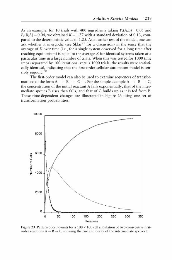
As an example, for 10 trials with 400 ingredients taking Pt(A,B)¼ 0.05 andPt(B,A)¼ 0.04, we obtained K¼ 1.27 with a standard deviation of 0.13, com-pared to the deterministic value of 1.25. As a further test of the model, one canask whether it is ergodic (see Sklar71 for a discussion) in the sense that theaverage of K over time (i.e., for a single system observed for a long time afterreaching equilibrium) is equal to the average K for identical systems taken at aparticular time in a large number of trials. When this was tested for 1000 timesteps (separated by 100 iterations) versus 1000 trials, the results were statisti-cally identical, indicating that the first-order cellular automaton model is sen-sibly ergodic.70

The first-order model can also be used to examine sequences of transfor-mations of the form A ! B ! C . For the simple example A ! B ! C,the concentration of the initial reactant A falls exponentially, that of the inter-mediate species B rises then falls, and that of C builds up as it is fed from B.These time-dependent changes are illustrated in Figure 23 using one set oftransformation probabilities.

0

0

2000

4000

6000

8000

10000

50 100 150 200 250 300 350

Num

ber

of C

ells

Iterations

Figure 23 Pattern of cell counts for a 100 100 cell simulation of two consecutive first-order reactions A!B!C, showing the rise and decay of the intermediate species B.

Solution Kinetic Models 239

The series model can be extended to longer series and to the inclusion ofreversibility to illustrate a variety of fundamental kinetic phenomena in anespecially simple and straightforward manner. Depending on the relative ratesemployed, one can demonstrate the classic kinetic phenomena of a rate-limit-ing step and preequilibrium,72 and one can examine the conditions needed forthe validity of the steady-state approximation commonly used in chemicalkinetics.70

Kinetic and Thermodynamic Reaction Control

Parallel competing reactions

A! B ½8A! C ½9

can be simulated.70 An especially interesting example is present when the reac-tions are reversible:

A !B ½10A !C ½11

With properly chosen transformation probabilities, cellular automata can beused to examine the conditions governing thermodynamic and kinetic controlof reactions.73 Knowledge of such conditions is an important element inorganic synthesis74,75 and is an important consideration for many industrialreactions.76,77 Figure 24 shows a reaction being modeled with the parametersPt(A,B)¼ 0.01, Pt(A,C)¼ 0.001, Pt(B,A)¼ 0.02, and Pt(C,A)¼ 0.0005, and aset of 10,000 ingredients. Starting with reactants A, the kinetically favoredproduct B is produced in excess in the initial stages of the reaction, whereasat later times the thermodynamically favored product C gains dominance.The number of interacting species (10,000) is rather large in this illustration,and the results of the cellular automata model are in good agreement withthose found in a deterministic, numerical solution for the same conditions.78

For example, the cellular automata model yields final, equilibrium concentra-tions for species B and C of [B]¼ 0.14390.0038 and [C]¼ 0.56950.0048compared to the reported deterministic values of 0.14 and 0.571, respectively.

Excited-State Kinetics

Another important application of the first-order model is the examina-tion of the ground- and excited-state kinetics of atoms and molecules.79 Thesesystems are characterized by competing first-order transitions representingboth radiative and nonradiative processes. The radiative processes normally

240 Cellular Automata Models of Aqueous Solution Systems

include light absorption from the ground state as well as fluorescence andphosphorescence originating from the excited states. The nonradiative pro-cesses include spin-allowed internal conversions and spin-forbidden inter-system crossings. The ‘‘species’’ in this case are the different atomic ormolecular electronic states involved, represented in the visualizations by differ-ent colors. Cellular automata models can be constructed to represent bothpulse conditions, which are normally used, for example, to determineexcited-state lifetimes, and steady-state conditions, which are customarilyemployed to determine spectra and the quantum yields of the processes takingplace. Pulse conditions are simulated by starting all the ingredients in a partic-ular excited state or in a distribution of excited states characteristic of a start-ing distribution created by some process of interest; the states are allowed todecay according to the transition probabilities appropriate to that system, and

Figure 24 Illustration of kinetic and thermodynamic reaction control: B is thekinetically favored product (higher probability of formation from A), and C is thethermodynamically favored product (greater equilibrium constant with A).

Solution Kinetic Models 241

the time evolutions of their populations are followed. Under pulse conditions,the decays eventually lead to a condition in which all of the ingredients arein the ground state (in the absence of additional trapping states). For steady-state conditions, additional transitions from the ground to the excited statesare introduced with appropriate transition probabilities.

One illustration of the excited-state cellular automata model is thedynamics of the excited-state transitions of oxygen atoms.80 The oxygenatom has a 3P ground state and 1S and 1D excited states. Emissions fromthe latter two excited states play an important role in the dramatic light dis-plays—the aurora borealis or ‘‘northern lights’’—seen under certain condi-tions in the northern polar skies and similar emissions have been detected inthe atmospheres of Mars and Venus. The excited states are believed to be pro-duced mainly by dissociative recombinations of ionized oxygen molecules andelectrons generated in the atmosphere by ultraviolet (UV) bombardment dur-ing the daylight hours.81,82

Oþ2 þ e ! O*þO** ½12

In this equation, the species O* and O** are unspecified atomic oxygen states,3P, 1S, or 1D. The most prominent feature in the atmospheric displays is nor-mally the green, spin-allowed 1S! 1D transition appearing at 5577 A.

Using transition probabilities taken from the compilation of Okabe,83

we simulated the dynamics associated with these atomic transitions underboth pulse and steady-state conditions. For the pulse simulations, two startingconditions were examined: the first in which all ingredients started in theupper 1S excited state, and the second in which the ingredients started in a dis-tribution believed characteristic of that produced by the dissociative recombi-nation process in Eq. [12].82 The simulations yield excited-state lifetimes andluminescence quantum yields consistent with the experimental observationsfor these properties. An interesting feature arising from these studies is the pos-sibility that a 1D/3P population inversion could occur under certain atmo-spheric conditions, as a result of the exceedingly long lifetime of the 1Dstate, estimated to be about 200 s.82

Second-Order Kinetics

Several groups have developed cellular automata models for particularreaction–diffusion systems. In particular, the Belousov–Zhabotinsky oscillat-ing reaction has been examined in a number of studies.84–86 Attention hasalso been directed at the AþB!C reaction, using both lattice-gasmodels 87–90 and a generalized Margolus diffusion approach.91 We developeda simple, direct cellular automaton model92 for hard-sphere bimolecular chem-ical reactions of the form

Aþ B! CþD ½13

242 Cellular Automata Models of Aqueous Solution Systems

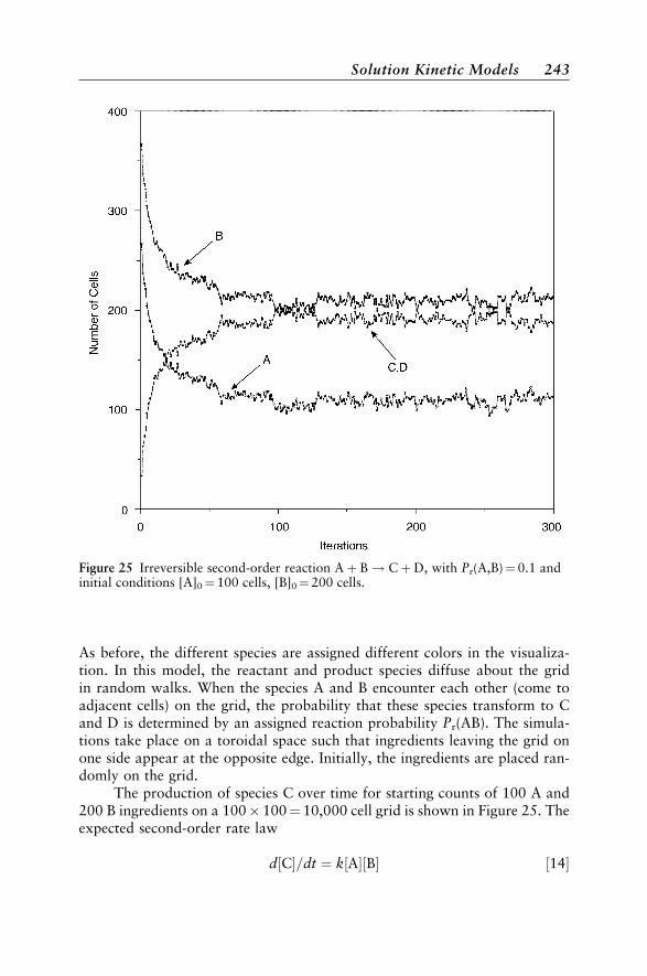
As before, the different species are assigned different colors in the visualiza-tion. In this model, the reactant and product species diffuse about the gridin random walks. When the species A and B encounter each other (come toadjacent cells) on the grid, the probability that these species transform to Cand D is determined by an assigned reaction probability Pr(AB). The simula-tions take place on a toroidal space such that ingredients leaving the grid onone side appear at the opposite edge. Initially, the ingredients are placed ran-domly on the grid.

The production of species C over time for starting counts of 100 A and200 B ingredients on a 100 100¼ 10,000 cell grid is shown in Figure 25. Theexpected second-order rate law

d½C=dt ¼ k½A½B ½14

Figure 25 Irreversible second-order reaction Aþ B! CþD, with Pr(A,B)¼ 0.1 andinitial conditions [A]0¼ 100 cells, [B]0¼ 200 cells.

Solution Kinetic Models 243

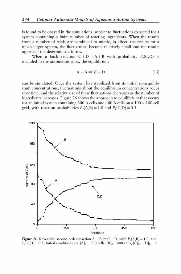
is found to be obeyed in the simulations, subject to fluctuations expected for asystem containing a finite number of reacting ingredients. When the resultsfrom a number of trials are combined to mimic, in effect, the results for amuch larger system, the fluctuations become relatively small and the resultsapproach the deterministic forms.

When a back reaction CþD!AþB with probability Pr(C,D) isincluded in the automaton rules, the equilibrium

Aþ B ! CþD ½15

can be simulated. Once the system has stabilized from its initial nonequilib-rium concentrations, fluctuations about the equilibrium concentrations occurover time, and the relative size of these fluctuations decreases as the number ofingredients increases. Figure 26 shows the approach to equilibrium that occursfor an initial system containing 300 A cells and 400 B cells on a 100 100 cellgrid, with reaction probabilities Pr(A,B)¼ 1.0 and Pr(C,D)¼ 0.5.

Figure 26 Reversible second-order reaction Aþ BÐ CþD, with Pr(A,B)¼ 1.0, andPr(C,D)¼ 0.5. Initial conditions are [A]0¼ 300 cells, [B]0¼ 400 cells, [C]0¼ [D]0¼ 0.

244 Cellular Automata Models of Aqueous Solution Systems

A variation of this theme occurs in a pseudo-first-order reaction. Thistype of reaction involves an actual second-order reaction, AþB!CþD, inwhich one of the reactants, say B, is present in sufficient excess that its varia-tion becomes effectively unnoticeable. Simulations with, for instance, 50 Aingredients and 1000 B ingredients, can bear out the expectation that the reac-tion kinetics are such that the rate of production of C and D appears to dependonly the concentration of A.

This second-order model is a first step toward the examination of morecomplex models that will include, for example, the influences of intermolecu-lar forces (departing from the hard-sphere ideal), solvent, temperature, andother features. Variations such as the inclusion of unstable intermediate spe-cies and additional reactions can also be simulated, so that, potentially, quitecomplex systems can be studied.

Enzyme Reactions

Many aqueous solution cellular automata models discussed earlier werecreated for systems in which there have been no changes in the states of anycells that model ingredients. Of great interest are the reactions catalyzed byenzymes, the engines of biochemical function. Some studies relating to thishave been reported,89,90 but more attention to this area of modeling wouldbe of value. A recent study on the kinetics of an enzyme reaction93 consideredthe Michaelis–Menten model shown in Eq. [16].

Eþ S ! ES! Eþ P ½16

Rules selected for this reaction included the joining and breaking probabilitiesas described earlier. In addition, it was necessary to include a probability ofconversion, Pc, of an enzyme–substrate pair, ES, to an enzyme–product pair,EP, that was programmed to be an irreversible event. The cells designated asenzymes, E, were not permitted to move, and their random distribution in thegrid limited them to a separation of at least 10 cells. Once a substrate moleculejoined with an enzyme, no other pairings were possible. The lipophilicity ofthe substrate and product molecules were varied using the PB(WS) and PB(WP)rules.

The dynamics were run for several concentrations of substrate and var-iations in the Pc values. Initial velocities of the reaction were recorded. TheMichaelis–Menten model was observed and characteristic Lineweaver–Burkplots were found from the model. Systematic variation of the lipophilicity ofsubstrates and products showed that a lower affinity between a substrate andwater leads to more of the S! P reaction at a common point along the reac-tion progress curve. This influence is greater than that of the affinity betweenthe substrate and the enzyme. The study created a model in which the morelipophilic substrates are more reactive. The water–substrate affinity appears

Solution Kinetic Models 245

to influence primarily the concentration of the ES complex at the observedpoint along the reaction progress curve. A low affinity between water and sub-strate favors a high ES concentration at this point. A hydrophilic substrateappears to be more entrapped in the water continuum, hence to be less avail-able to the enzyme. It was also observed that an accumulation of productmolecules around the enzymes coincides with a decline in the reaction rate.

An Anticipatory Model

An anticipatory system is one in which information is sent from an ele-ment in the early stages of a sequence of events to a nonacting element thatwill arise in that sequence. The information sent ahead prepares the future ele-ment to function based on information arising in advance of the normalsequence of events. The unmanifested element anticipates its ultimate manifes-tation in the sequence. An anticipatory system has been modeled by Kier andCheng94 using the dynamic characteristics of cellular automata. A concentra-tion of an intermediate product influences the creation of a supplementalenzyme that enhances the competence of an enzyme downstream. This antici-pation of a future event creates a condition in which the concentration of alater substrate is suppressed, a property characteristic of the system.

The anticipatory model employed in this study had the following step-wise reactions.

Aþ e1 ! Ae1 ! Be1 ! Bþ e1 ½17

Equation [17] is the conversion of A to B, assuming an irreversible first-orderreaction catalyzed by the enzyme e1. The rules governing the initial encounter,PB(Ae1) and J(Ae1), are set at the beginning of each run. The next step in thereaction is modeled as shown in Eqs. [18].

Bþ e2 !Be2 ! Ce2 ! Cþ e2 ½18aBe2 ! Ce2;4 ! Cþ e2;4 ½18b

If the system is not an anticipatory one, the conversion of Be2 to Ce2 wouldfollow only one route. If the system is anticipatory, as shown, there are twopaths for the conversion of Be2. The formation of e2,4 represents an enzymethat may function upon substrates B or D (Eqs. [19] and [20]).

Cþ e3 ! Ce3 ! De3 ! Dþ e3 ½19Dþ e4=e2;4 ! De4=e2;4 ! Ee4=e2;4 ! Eþ e4=e2;4 ½20

Thus the available enzyme to convert B to C is the same for an anticipatory ornonanticipatory system. In the case of an anticipatory system, there is formed,in advance of the creation of substrate D an enzyme, e2,4, that will enhance the

246 Cellular Automata Models of Aqueous Solution Systems

reaction of D and e4 to form product E. Substrate B serves as a predictor of theconcentration of D, reducing its accumulation, relative to that in a nonantici-patory system. Substrate D is confronted with an enhanced competence of itsspecific enzyme, modeled by e4 and e2,4 facilitating the conversion of D to E.The decrease in the concentration of D is the property of the anticipatory sys-tem that is created by the feed-forward influence of e2,4.

In each study, the dynamics revealed concentrations over time that areinfluenced by the presence or absence of a feed-forward or preadaption statein the system. The concentration of A steadily diminishes as successive concen-trations of B, C, and D rise and fall at the same levels. The concentration of Erises at the end of the run, eventually becoming the only ingredient in the sys-tem. The concentration of D is ca. 0.25 in a nonanticipatory model. In con-trast, with an anticipatory or feed-forward step in the system there is createdan additional amount of enzyme specific for substrate D (enzyme, e2,4) that isavailable at a future time to catalyze the conversion of D to E. This anticipa-tory attribute creates a property of the system in which the concentration ofingredient D is not allowed to accumulate to its normal level. In contrast, theconcentration of D in an anticipatory model is approximately 0.13, about halfthe D concentrations for the nonanticipatory models. The concentration of Btherefore serves as a predictor of the concentration of D at a later time.

Chromatographic Separation

Models of chromatographic separation based on cellular automata havebeen reported.95 Solvent cells were randomly distributed over the grid at theinitiation of each run. These 5230 cells, designated W, constituted 69% of thecells in the grid before the introduction of any other ingredients. The station-ary phase, designated B, was simulated by the presence of cells distributed ran-domly over the grid, replacing 600 W cells. The B cells were immobile andwere positioned at least three cells from another B cell. The solute cells, usuallysimulating a mixture of two different compounds, were represented by 10 cellseach. These solutes replace a corresponding number of W cells and were posi-tioned initially on the first row of the column.

The movements of the solutes and mobile phase in the grid were gov-erned by rules denoting the joining and breaking of like or unlike cells. Thegravity term was applied uniformly to all ingredients except the stationary-phase cells. The position of each solute cell was recorded at a given row inthe ‘‘chromatographic’’ column after a certain number of iterations. Each runwas repeated 100 times to achieve an average position on the column for 1000cells of a certain solute. The position of the peak maximum was determined bysumming the number of cells found in contiguous groups of 10 rows on thecolumn. These averages were then plotted against the iteration time.

The gravity parameter for each ingredient in the simulation definesthe flow rate. The polarity of the solvent, W, is encoded in the relative

Solution Kinetic Models 247

self-association experienced, which in turn is governed by the rules, PB(W) andJ(W). High values of PB(W) and low values of J(W) simulate a weak self-asso-ciation, corresponding to a relatively nonpolar solvent. The migration of thesolutes was found to be faster when the solvent was nonpolar. Another studyin the same paper95modeled the influence of the relative affinities of solutes forthe stationary phase B. This affinity is encoded in the parameters PB(SB) andJ(SB). High values of PB(SB) and low values of J(SB) denote a weak affinity.These parameters characterize the structural differences among solutes thatgive rise to different migratory rates and separations in chromatography.These studies revealed that solutes with a greater affinity for the stationaryphase migrated at a slower rate.

The effect of solvating the stationary phase was significant because thisproperty reflects the variability of this ingredient in the selection of suitablesolvents for experimental work. The variation in this property was encodedinto the PB(WB) and J(WB) parameters. A low value for the PB(WB) and ahigh value for the J(WB) parameters denotes a strong affinity of the solvent,W, for the stationary phase B. The study revealed a modest influence of theparameters on migration through the ‘‘column’’ but a greater influence onthe relative resolution among the two solutes in each study. The greater therelative solvation of the stationary phase, the poorer the resolution.

CONCLUSIONS

The examples given here illustrate some of the capabilities that cellularautomata models have for enhancing our understanding of complex, dynamicsystems in chemistry.96 They also give a hint of some of the potential richnessthat these models may hold for the future. The limitations of the cellular auto-mata models are quite clear: they do not make use of the customary tools ofthe trade—the molecular structures, the force fields, the energetic calculations,and their associated equations—that are so firmly embedded in our trainingand experience as computational chemists. Yet the absence of these toolsalso contributes to the strength of the method. In the absence of these tools,the modeler is forced to design appropriate ‘‘rules’’ that encapsulate the natureof things, thereby making the modeler an active participant in the process ofunderstanding the complex systems under investigation. The heuristic rules,moreover, yield models that have an attractive simplicity, are computationallyundemanding, and are readily visualizable. They also enable, in many cases, aparsing of the influences in a complex system—say, changing the temperatureof one component and not of another—that can lead both to a better under-standing of how these factors influence behavior and to the discovery of newinsights and possibilities.

The cellular automata models described here contained some novel tech-niques for this paradigm. The use of a gravity rule to set the stage for the

248 Cellular Automata Models of Aqueous Solution Systems

demixing of immiscible liquids is one example. Another is the use of a varie-gated cell with independent states and trajectory rules for each of the fourfaces. These innovations have greatly enhanced the potential for cellular auto-mata models to explore new areas of dynamic systems.

We close with two quotations. The first describes in a general way boththe limitations and the promise of modeling work:97 ‘‘Because models of thissort may provide an unjustified sense of verisimilitude, it is important to recog-nize them for what they are: imitations of reality that represent at best indivi-dual realizations of complex processes in which stochasticity, contingency,and non-linearity underlie a diversity of possible outcomes. Individual simula-tions cannot be taken as more than representative of this diversity, butrepeated simulations can provide statistical ensembles that contain robust ker-nels of truth.’’ The second quote positions the models between theory andexperiment:98 ‘‘It is worthwhile to emphasize that the computer based modelsoffer a half-way house between theory and experiment. They have the rigor ofmathematical models without the generality, while allowing the selection andrepeatability of good, critical experiments without the enforced connection toreality.’’

APPENDIX

The computations were done on personal computers using a suite of pro-grams called DING HAO. The programs are written in C.

Computing the Moving Probability

The moving probability is defined as follows:

Let A be a molecule and let S be the set of directions in which the jcell [see Figure 5(a)] of A is empty. Let n be the number of empty jneighbors [see Figure 5(a)] of A. We describe the computed directionbreaking probability at d direction, written as dirPB(d), as: dirPB(d)¼ 1if the j cell at A’s d direction is empty, dirPB(d)¼PB(AB) otherwise,where B is the molecule at the j cell in the d direction of A.

Let Q be the product of dirPB(d) for all d in S.

Let J(d)¼ 1 if the k cell and the j cell [see Figure 5(c)] at A’s d directionare empty, J(d)¼ J(AB)þ y if only the j cell at A’s d direction is empty,and the k cell at A’s d direction is occupied by the molecule B, where y ¼absG(A) if d¼ south, y¼ 0 otherwise. Then y¼GD(AB) if the j cell at A’sd direction is occupied by the molecule B. Furthermore, in this case, nshould be incremented by 1.

Appendix 249

Let temp¼ (n/Q)1, if Q> 0.

Let MP(d) be the probability of moving in a direction d and define itas follows:

MPðdÞ ¼ f=½1þ temp =JðdÞ if Q>0, where f is the free movementprobability of A, MPðdÞ ¼ 0 otherwise.

Let MP be the sum of MP(d) for all four directions.

Normalize MP(d) if it is necessary. That is, change MPðdÞ to MPðdÞ=MPfor all directions d if MP>1.

We choose this method to compute the moving probability because:

1. It allows a simple computation.2. It allows the influence of k cells, but the effect is limited so that the

influence of one direction does not overshadow the influence from otherdirections.

3. When JðABÞ ¼ 1, and all adjacent j cells to the occupant are empty, theprobability of moving in any direction is 0.25 of its free movementprobability. This reduced joining parameter agrees with the intuitivelyreasonable assumption that any occupant should not be biased on anydirection (unless gravity is considered).

The directional moving probabilities are computed for various configura-tions and rules, giving the results in Figures 7–10.

REFERENCES

1. J. I. Steinfeld, J. S. Francisco, and W. L. Hase, Chemical Kinetics and Dynamics, Prentice Hall,Englewood Cliffs, NJ, 1989.

2. A. Papoulis, Probability, Random Variables, and Stochastic Processes, McGraw-Hill, NewYork, 1991.

3. D. T. Gillespie, J. Phys. Chem., 81, 2340 (1977). Exact Stochastic Simulation of CoupledChemical Reactions.

4. D. T. Gillespie, J. Chem. Phys., 72, 5363 (1980). Approximating the Master Equation byFokker–Planck-type Equations for Single-Variable Chemical Systems.

5. D. T. Gillespie, J. Comput. Phys., 22, 403 (1976). A General Method for NumericallySimulating the Stochastic Time Evolution of Coupled Chemical Reactions.

6. J. Shi and J. R. Barker, Int. J. Chem. Kinetics, 22, 187 (1990). Incubation in CyclohexaneDecomposition at High Temperatures.

7. L. Vereecken, G. Huyberechts, and J. Peeters, J. Chem. Phys., 106, 6564 (1997). StochasticSimulation of Chemically Activated Unimolecular Reactions.

8. J. M. Haile, Molecular Dynamics Simulations: Elementary Methods, Wiley, New York, 1992,pp. 11–18.

9. M. P. Allen and D. J. Tildesley, Computer Simulations of Liquids, Oxford University Press,New York, 1987.

10. W. L. Jorgensen, in Encyclopedia of Computational Chemistry, P. v. R. Schleyer, Ed., Wiley,New York, 1998, pp. 1754–1763. Monte Carlo Simulations for Liquids.

250 Cellular Automata Models of Aqueous Solution Systems

11. H. Meirovitch, in Reviews in Computational Chemistry, K. B. Lipkowitz and D. B. Boyd,Eds., Wiley-VCH, New York, 1998, Vol. 12, pp. 1–74. Calculation of the Free Energy andthe Entropy of Macromolecular Systems by Computer Simulation. T. P. Lybrand, in Reviewsin Computational Chemistry, K. B. Lipkowitz and D. B. Boyd, Eds., VCH Publishers, NewYork, 1990, Vol. 1, pp. 295–320. Computer Simulation of Biomolecular Systems UsingMolecular Dynamics and Free Energy Perturbation Methods.

12. S. M. Ulam, Proc. Int. Congr. Math. (held in 1950), 2, 264 (1952). Random Processes andTransformations.

13. S. M. Ulam, Adventures of a Mathematician, Charles Scribner’s Sons, New York, 1976.

14. J. von Neumann, Theory of Self-Replicating Automata, A. Burks, Ed., University of IllinoisPress, Urbana, 1966.

15. K. Zuse, Int. J. Theoret. Phys., 21, 589 (1982). The Computing Universe.

16. T. Toffoli and N. Margolus, Cellular Automata Machines, MIT Press, Cambridge, MA, 1987.

17. M. Schroeder, Fractals, Chaos, Power Laws, W. H. Freeman, New York, 1991, p. 371.

18. J. Signorini, in Cellular Automata and Modeling of Complex Physical Systems, P. Manneville,N. Boccara, G. Y. Vishniac, and R. Bidaux, Eds., Springer-Verlag, New York, 1990, pp. 57–70. Complex Computing with Cellular Automata.

19. G. Y. Vichniac, Physica D, 10, 96 (1984). Simulating Physics with Cellular Automata.

20. T. Toffoli, Physica D, 10, 117 (1984). Cellular Automata as an Alternative (Rather than anApproximation of) Differential Equations in Modeling Physics.

21. S. Wolfram, Physica D, 10, vii (1984) Preface.

22. S. Kauffman, Physica D, 10, 145 (1984). Emergent Properties in Random Complex Auto-mata.

23. S. Wolfram, Ed., Theory and Applications of Cellular Automata, World Scientific, Singapore,1986.

24. R. J. Gaylord and K. Nishidate, Modeling Nature: Cellular Automata Simulations, Springer-Verlag, New York, 1996.

25. H. Gutowitz, Cellular Automata: Theory and Experiment, MIT Press, Cambridge, MA,1991.

26. R. Kapral and K. Showalter, Chemical Waves and Patterns, Kluwer, Dordrecht, 1995.

27. G. B. Ermentrout and L. Edelstein-Keshet, J. Theor. Biol., 160, 97 (1993). Cellular AutomataApproaches to Biological Modeling.

28. B. Chopard, M. Droz, and B. Chopard, Cellular Automata Modeling of Physical Systems,Cambridge University Press, Cambridge, UK, 1998.

29. L. B. Kier and B. Testa, Adv. Drug Res., 26, 1 (1995). Complexity and Emergence in DrugResearch.

30. A. Geiger, F. H. Stillinger, and A. Rahman, J. Phys. Chem., 70, 4186 (1979). Aspects of thePercolation Process for Hydrogen Bonded Networks in Water.

31. I. Ohmine and H. Tanaka, Chem. Rev., 93, 2545 (1993). Fluctuation, Relaxations andHydration in Liquid Water, Hydrogen Bond Rearrangement Dynamics.

32. M. Mezei and D. L. Beveridge, J. Chem. Phys., 74, 622 (1981) Theoretical Studies ofHydrogen Bonding in Liquid Water and Aqueous Solutions.

33. P. L. M. Plummer, J. Mol. Struct., 23, 47 (1991). Molecular Dynamics Simulations andQuantum Mechanical Studies of the Hydrogen Bond in Water Cluster Systems.

34. P. J. Rossky and M. Karplus, J. Am. Chem. Soc., 101, 1913 (1979). Solvation. A MolecularDynamics Study of a Dipeptide in Water.

35. S. A. Rice and M. G. Skeats, J. Phys. Chem., 85, 1108 (1981). A Random Network Model forWater.

36. L. B. Kier and C.-K. Cheng, J. Chem. Inf. Comput. Sci., 34, 647 (1994). A Cellular AutomataModel of Water.

References 251

37. R. L. Blumberg, G. Shlifer, and H. E. Stanley, J. Phys. A: Math. Gen., 13, L 147 (1980). MonteCarlo Tests of the Universality in a Correlated-Site Percolation Problem.

38. M. H. Brodsky and P. H. Leary, Bull. Am. Phys. Soc., 25, 260 (1980). The TemperatureDependence of the Refractive Index of Hydrogenated Amorphous Silicon and Implicationsfor Electroreflectance.

39. G. E. Walrafen, in Structure of Water, Hydrogen-Bonded Systems A. K. Covingtonand P. Jones, Eds., Taylor and Francis, London, UK, 1968, pp. 173–175. Structure of Water.

40. G. H. Haggis, J. B. Hasted, and T. J. Buchanan, J. Phys. Chem., 54, 1452 (1952). TheDielectric Properties of Water in Solutions.

41. W. A. P. Luck, Acta Chim. Hung. Acad. Sci., 121, 119 (1986). Role of Hydrogen Bonding inthe Structure of Liquids.

42. L. B. Kier, C.-K. Cheng, and B. Testa, Pharm. Res., 12, 1521 (1995). A Cellular AutomataModel of Dissolution.

43. L. B. Kier and C.-K. Cheng, J. Math. Chem., 21, 71 (1997). A Cellular Automata Model of theSoluble State.

44. L. B. Kier, C.-K. Cheng, and B. Testa, Pharm. Res., 12, 615 (1995). A Cellular AutomataModel of the Hydrophobic Effect.

45. W. L. Jorgensen, J. Gao, and C. Ravimohan, J. Phys. Chem., 89, 3470 (1985). Monte CarloSimulations of Alkanes in Water: Hydration Numbers and Hydrophobic Effect.

46. W. Blokzijl and J. B. F. N. Engberts, Angew. Chem. Int. Ed. Engl., 32, 1545 (1993).Hydrophobic Effects, Opinions and Facts.

47. G. Hummer, S. Garde, A. E. Garcia, A. Pohorille, and L. R. Pratt, Proc. Natl. Acad. Sci. USA,93, 8951 (1996). An Information Theory Model of Hydrophobic Interaction.

48. B. J. Berne, Proc. Natl. Acad. Sci. USA, 93, 8800 (1996). Inferring the HydrophobicInteraction from the Properties of Neat Water.

49. L. B. Kier, C.-K. Cheng, and B. Testa, J. Pharm. Sci., 86, 774 (1997). A Cellular AutomataModel of Diffusion in Aqueous Systems.

50. C. M. Gary-Bobo and H. W. Weber, J. Phys. Chem., 73, 1155 (1969). Diffusion of Alcoholsand Amides in Water from 4 to 37.

51. S. B. Horowitz and I. R. Fenichel, J. Phys. Chem., 68, 3378 (1964). Solute DiffusionalSpecificity in Hydrogen Bonding Systems.

52. C.-K. Cheng and L. B. Kier, J. Chem. Inf. Comput. Sci., 35, 1054 (1995). A Cellular AutomataModel of Oil–Water Partitioning.

53. L. B. Kier and C.-K. Cheng, in Lipophilicity in Drug Action and Toxicity, V. Pliska, B. Testa,and H. van de Waterbeemd, Eds., VCH Publishers, Weinheim, Germany, 1996, pp. 187–192. A Cellular Automata Model of Partitioning Between Liquid Phase.

54. I. Benjamin, J. Phys. Chem., 97, 1432 (1992). Theoretical Studies of Water/1,2-Dichloro-ethane Interface: Structure, Dynamics and Conformational Equilibria at the Liquid–LiquidInterface.

55. I. L. Carpenter and W. J. Hebre, J. Chem. Phys., 94, 531 (1990). A Molecular Dynamics Studyof the Hexane/Water Interface.

56. J. Gao and W. L. Jorgensen, J. Phys. Chem., 92, 5813 (1988). Theoretical Examination ofHexanol/Water Interfaces.

57. P. Luise, J. Chem. Phys., 86, 4177 (1987). Monte Carlo Simulation of Liquid–Liquid Benzene/Water Interface.

58. M. Meyer, M. Mareschal, and M. Hayoun, J. Chem. Phys., 89, 1067 (1988). ComputerModeling of a Liquid Interface.

59. B. Smit, P. A. J. Hilbers, K. Esselink, L. A. M. Rubert, N. M. van Os, and A. Schlijper, J. Phys.Chem., 59, 6361 (1991). Structure of a Water/Oil Interface in the Presence of Micelles: AComputer Simulation Study.

252 Cellular Automata Models of Aqueous Solution Systems

60. M. N. Jones and D. Chapman, Micelles, Monolayers, Biomembranes, Wiley, New York,1994.

61. P. Mukergee and K. J. Mysels, Critical Micelle Concentration in Aqueous Surfactant Systems,National Bureau of Standards, Washington, DC, 1971.

62. L. B. Kier, C.-K. Cheng, and B. Testa, Pharm. Res., 13, 1419 (1996). A Cellular AutomataModel of Micelle Formation.

63. L. Espada, M. N. Jones, and G. Pilcher, J. Chem. Thermo., 12, 1 (1970). Enthalpy ofMicellization of d-Dodecyltrimethyl Ammonium Bromide.

64. T. Ingram and M. N. Jones, J. Chem. Soc., 65, 297 (1969). Membrane Potential Studies onSurfactant Solution.

65. L. B. Kier and C.-K. Cheng, J. Theor. Biol., 186, 75 (1997). A Cellular Automata Model ofMembrane Permeability.

66. A. Walter and J. Gutknect, J. Membr. Biol., 90, 207 (1986). The Movement of MoleculesAcross Lipid Membranes: A Molecular Theory.

67. L. B. Kier, C.-K. Cheng, M. Tute, and P. G. Seybold, J. Chem. Inf. Comput. Sci., 38, 271(1998). A Cellular Automata Model of Acid Dissociation.

68. G. B. Barlin and D. D. Perrin Quart. Rev. Chem. Soc., 20, 75 (1966). Prediction of theStrength of Organic Acids.

69. L. B. Kier, C.-K. Cheng, and B. Testa, J. Chem. Inf. Comput. Sci., 39, 32 (1999). A CellularAutomata Model of the Percolation Process.

70. P. Seybold, L. B. Kier, and C.-K. Cheng, J. Chem. Inf. Comput. Sci., 37 386 (1997).Simulation of First-Order Chemical Kinetics Using Cellular Automata.

71. L. Sklar, Physics and Chance, Cambridge University Press, New York, 1993.

72. P. Atkins, Physical Chemistry, 6th ed., Freeman, New York, 1998, pp. 778–783.

73. A. Neuforth, P. G. Seybold, L. B. Kier, and C.-K. Cheng, Int. J. Chem. Kinetics, 32, 529(2000). Cellular Automata Models of Kinetically and Thermodynamically ControlledReactions.

74. J. D. Roberts and M. C. Caserio, Basic Principles of Organic Chemistry, 2nd ed., Benjamin,New York, 1977, pp. 374–376.

75. K.-C. Lin, J. Chem. Educ., 65, 857 (1988). Understanding Product Optimization.

76. G. N. Vriens, Industr. Eng. Chem., 46, 669 (1954). Kinetics of Coupled Reversible Reactions.

77. A. P. Gelbein, CHEMTECH, Sept., 1998, p. 1. Thinking Out of the Box.

78. M. E. Brown, K. J. Buchanan, and A. Goosen, J. Chem. Educ., 62, 575 (1985). Thermo-dynamically and Kinetically Controlled Products.

79. P. G. Seybold, L. B. Kier, and C.-K. Cheng, J. Phys. Chem., 102, 886 (1998). StochasticCellular Automata Models of Molecular Excited-State Dynamics.

80. P. G. Seybold, L. B. Kier, and C.-K. Cheng, Int. J. Quantum Chem., 75, 751 (1999). AuroraBorealis: Stochastic Cellular Automata. Simulations of the Excited-State Dynamics ofOxygen Atoms.

81. S. L. Guberman, Science, 278, 1276 (1997). Mechanism for the Green Glow of the UpperAtmosphere.

82. D. Kella, L. Vejby-Christiansen, P. J. Johnson, H. B. Peterson, and L. H. Andersen, Science,276, 1530 (1997). The Source of Green Light Emission Determined from a Heavy-AtomStorage Ring Experiment.

83. H. Okabe, Photochemistry of Small Molecules, Wiley, New York, 1978, p. 370.

84. R. Kapral and K. Showalter, Eds., Chemical Waves and Patterns, Kluwer, Dordrecht, TheNetherlands, 1995.

85. R. Kapral and X.-G. Wu, J. Phys. Chem., 100, 18976 (1996). Stochastic Description ofTemporal and Spatial Dynamics of Far-From Equilibrium Reactions.

References 253

86. V. K. Vanag, J. Phys. Chem., 100, 11336 (1996). Probability Cellular Automaton-AidedModeling of the Stirring Effect in the Autocatalytic Step of the Belousov–ZhabotinskyReaction.

87. B. Chopard and M. Droz, Cellular Automata Modeling of Physical Systems, CambridgeUniversity Press, Cambridge, UK, 1998.

88. B. Chopard and M. Droz, Europhysics Lett., 15, 459 (1991). Microscopic Study of theProperties of the Reaction Front in an Aþ B! C Reaction-Diffusion System.

89. S. Cornell, M. Droz, and B. Chopard, Phys. Rev. A, 44, 4826 (1991). Role of Fluctuations forInhomogeneous Reaction-Diffusion Phenomena.

90. S. Cornell, M. Droz, and B. Chopard, Physica A, 188, 322 (1992). Some Properties of theDiffusion-Limited Reaction nAþmB! C with Homogeneous and Inhomogeneous InitialConditions.

91. H. S. Berryman and D. R. Franceschetti, Phys. Lett. A, 136, 348 (1989). Simulation ofDiffusion Controlled Reaction Kinetics Using Cellular Automata.

92. J. P. Moore, P. G. Seybold, L. B. Kier, and C.-K. Cheng, to be published. Second OrderReactions Simulated by Cellular Automata.

93. L. B. Kier, C.-K. Cheng, and B. Testa, J. Mol. Graphics, 14, 227 (1996). A Cellular AutomataModel of Enzyme Kinetics.

94. L. B. Kier and C.-K. Cheng, J. Mol. Graphics Modelling, 18, 29 (2000). A Cellular AutomataModel of an Anticipatory System.

95. L. B. Kier, C.-K. Cheng, and T. Karnes, J. Biol. Chromatogr., 14, 530 (2000). A CellularAutomata Model of Chromatographic Separation.

96. L. B. Kier, C.-K. Cheng, and P. G. Seybold, SAR QSAR Environ. Res., 11, 79 (2000). CellularAutomata Models of Chemical Systems.

97. S. A. Levin, B. Grenfell, A. Hastings, and A. S. Perelson, Science, 275, 335 (1997).Mathematical and Computational Challenges in Popululation Biology and EcosystemScience.

98. J. H. Holland. Emergence, Perseus Books, Reading, MA, 1998.

254 Cellular Automata Models of Aqueous Solution Systems

APPENDIX

Books Published on the Topicsof Computational Chemistry

Kenny B. Lipkowitz and Donald B. Boyd

Department of Chemistry, Indiana University-Purdue Universityat Indianapolis (IUPUI), Indianapolis, Indiana 46202-3274

INTRODUCTION

Computational chemistry is at the intersection of chemistry, mathe-matics, computer science, physics, library science, biology, and materialsscience. Although computational chemistry borrows from and contributes tothese other sciences, it can be considered in its own right as a well-defined dis-cipline for several reasons including having its own representation as the Com-puters in Chemistry division of the American Chemical Society, a GordonResearch Conference,1 university courses, a five-volume encyclopedia,2 andmany journals targeted at all or parts of computational chemistry. The disci-pline has gained both recognition and respect over the years.

Although computational chemistry, in one form or another, has beenaround for 50 or so years, the crystallization of this area of science has takenplace only in the last 20 to 25 years. During the past decade, the importance ofcomputational chemistry has grown considerably. Indeed, this was one of thereasons for creating Reviews in Computational Chemistry; there existed aneed for bringing to this audience reviews, tutorials, advances, and informa-tion related to what we do as a group.

As editors, we occasionally receive inquiries from around the world onvarious aspects of the field. One question we get is what publications andbooks exist in our field. A common scenario involves a molecular modeler

Reviews in Computational Chemistry, Volume 17Kenny B. Lipkowitz and Donald B. Boyd, Editors

Wiley-VCH, John Wiley and Sons, Inc., New York, 2001

Reviews in Computational Chemistry, Volume 17. Edited by Kenny B. Lipkowitz, Donald B. BoydCopyright 2001 John Wiley & Sons, Inc.

ISBNs: 0-471-39845-4 (Hardcover); 0-471-22441-3 (Electronic)

255

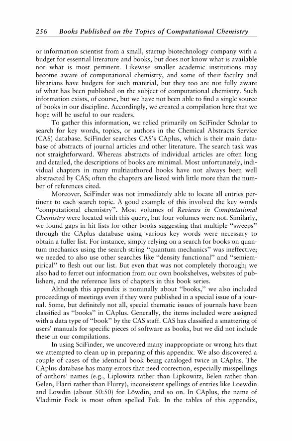
or information scientist from a small, startup biotechnology company with abudget for essential literature and books, but does not know what is availablenor what is most pertinent. Likewise smaller academic institutions maybecome aware of computational chemistry, and some of their faculty andlibrarians have budgets for such material, but they too are not fully awareof what has been published on the subject of computational chemistry. Suchinformation exists, of course, but we have not been able to find a single sourceof books in our discipline. Accordingly, we created a compilation here that wehope will be useful to our readers.

To gather this information, we relied primarily on SciFinder Scholar tosearch for key words, topics, or authors in the Chemical Abstracts Service(CAS) database. SciFinder searches CAS’s CAplus, which is their main data-base of abstracts of journal articles and other literature. The search task wasnot straightforward. Whereas abstracts of individual articles are often longand detailed, the descriptions of books are minimal. Most unfortunately, indi-vidual chapters in many multiauthored books have not always been wellabstracted by CAS; often the chapters are listed with little more than the num-ber of references cited.

Moreover, SciFinder was not immediately able to locate all entries per-tinent to each search topic. A good example of this involved the key words‘‘computational chemistry’’. Most volumes of Reviews in ComputationalChemistry were located with this query, but four volumes were not. Similarly,we found gaps in hit lists for other books suggesting that multiple ‘‘sweeps’’through the CAplus database using various key words were necessary toobtain a fuller list. For instance, simply relying on a search for books on quan-tum mechanics using the search string ‘‘quantum mechanics’’ was ineffective;we needed to also use other searches like ‘‘density functional’’ and ‘‘semiem-pirical’’ to flesh out our list. But even that was not completely thorough; wealso had to ferret out information from our own bookshelves, websites of pub-lishers, and the reference lists of chapters in this book series.

Although this appendix is nominally about ‘‘books,’’ we also includedproceedings of meetings even if they were published in a special issue of a jour-nal. Some, but definitely not all, special thematic issues of journals have beenclassified as ‘‘books’’ in CAplus. Generally, the items included were assignedwith a data type of ‘‘book’’ by the CAS staff. CAS has classified a smattering ofusers’ manuals for specific pieces of software as books, but we did not includethese in our compilations.

In using SciFinder, we uncovered many inappropriate or wrong hits thatwe attempted to clean up in preparing of this appendix. We also discovered acouple of cases of the identical book being cataloged twice in CAplus. TheCAplus database has many errors that need correction, especially misspellingsof authors’ names (e.g., Liplowitz rather than Lipkowitz, Belen rather thanGelen, Flarri rather than Flurry), inconsistent spellings of entries like Loewdinand Lowdin (about 50:50) for Lowdin, and so on. In CAplus, the name ofVladimir Fock is most often spelled Fok. In the tables of this appendix,

256 Books Published on the Topics of Computational Chemistry

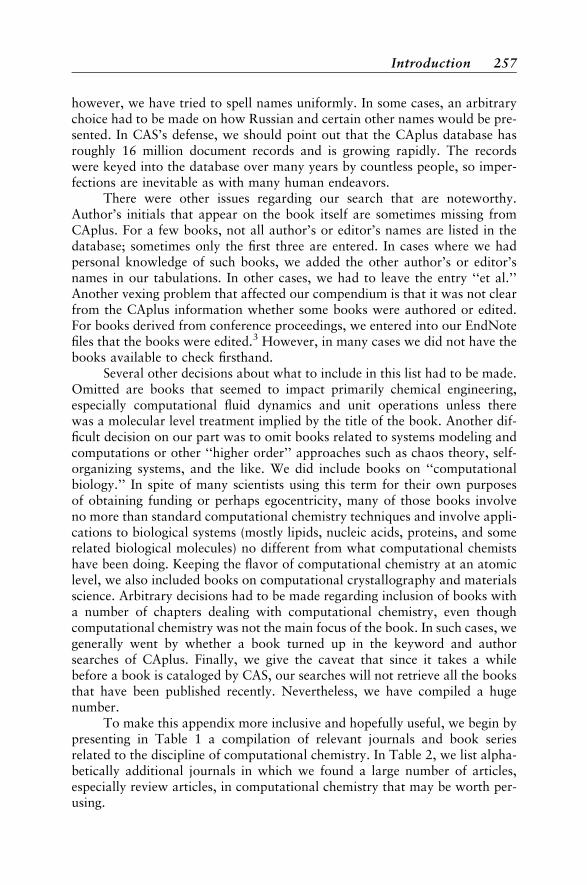
however, we have tried to spell names uniformly. In some cases, an arbitrarychoice had to be made on how Russian and certain other names would be pre-sented. In CAS’s defense, we should point out that the CAplus database hasroughly 16 million document records and is growing rapidly. The recordswere keyed into the database over many years by countless people, so imper-fections are inevitable as with many human endeavors.

There were other issues regarding our search that are noteworthy.Author’s initials that appear on the book itself are sometimes missing fromCAplus. For a few books, not all author’s or editor’s names are listed in thedatabase; sometimes only the first three are entered. In cases where we hadpersonal knowledge of such books, we added the other author’s or editor’snames in our tabulations. In other cases, we had to leave the entry ‘‘et al.’’Another vexing problem that affected our compendium is that it was not clearfrom the CAplus information whether some books were authored or edited.For books derived from conference proceedings, we entered into our EndNotefiles that the books were edited.3 However, in many cases we did not have thebooks available to check firsthand.

Several other decisions about what to include in this list had to be made.Omitted are books that seemed to impact primarily chemical engineering,especially computational fluid dynamics and unit operations unless therewas a molecular level treatment implied by the title of the book. Another dif-ficult decision on our part was to omit books related to systems modeling andcomputations or other ‘‘higher order’’ approaches such as chaos theory, self-organizing systems, and the like. We did include books on ‘‘computationalbiology.’’ In spite of many scientists using this term for their own purposesof obtaining funding or perhaps egocentricity, many of those books involveno more than standard computational chemistry techniques and involve appli-cations to biological systems (mostly lipids, nucleic acids, proteins, and somerelated biological molecules) no different from what computational chemistshave been doing. Keeping the flavor of computational chemistry at an atomiclevel, we also included books on computational crystallography and materialsscience. Arbitrary decisions had to be made regarding inclusion of books witha number of chapters dealing with computational chemistry, even thoughcomputational chemistry was not the main focus of the book. In such cases, wegenerally went by whether a book turned up in the keyword and authorsearches of CAplus. Finally, we give the caveat that since it takes a whilebefore a book is cataloged by CAS, our searches will not retrieve all the booksthat have been published recently. Nevertheless, we have compiled a hugenumber.

To make this appendix more inclusive and hopefully useful, we begin bypresenting in Table 1 a compilation of relevant journals and book seriesrelated to the discipline of computational chemistry. In Table 2, we list alpha-betically additional journals in which we found a large number of articles,especially review articles, in computational chemistry that may be worth per-using.

Introduction 257

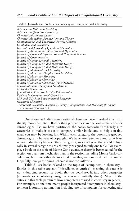
Our efforts at finding computational chemistry books resulted in a list ofslightly more than 1600. Rather than present these in one long alphabetical orchronological list, we have partitioned the books somewhat arbitrarily intocategories to make it easier to compare similar books and to help you findwhat you may be looking for. Within each category, the books are groupedchronologically by year of copyright. We have attempted to avoid or at leastreduce redundancy between these categories, so some books that could fit logi-cally in several categories are arbitrarily assigned to only one table. For exam-ple, a book on the topic of Monte Carlo quantum theory is better suited for thesection on quantum mechanics than in the section including Monte Carlo cal-culations, but some other decisions, akin to this, were more difficult to make.Hopefully, our partitioning scheme is not too inflexible.

Table 3 lists books related to the topic of ‘‘computers in chemistry’’.Entries in this table are not ‘‘miscellaneous entries’’, meaning this table isnot a dumping ground for books that we could not fit into other categories(although some arbitrary assignment was admittedly done). Most of theentries in this table pertain to how computers are used in chemistry in general.For example, at one time many people interpreted ‘‘computers in chemistry’’to mean laboratory automation including use of computers for collecting and

Table 1 Journals and Book Series Focusing on Computational Chemistry

Advances in Molecular ModelingAdvances in Quantum ChemistryChemical Informatics LettersChemical Modelling: Applications and TheoryComputational and Theoretical Polymer ScienceComputers and ChemistryInternational Journal of Quantum ChemistryJournal of Biomolecular Structure and DynamicsJournal of Chemical Information and Computer ScienceJournal of ChemometricsJournal of Computational ChemistryJournal of Computer-Aided Materials DesignJournal of Computer-Aided Molecular DesignJournal of Mathematical ChemistryJournal of Molecular Graphics and ModellingJournal of Molecular ModelingJournal of Molecular StructureJournal of Molecular Structure: THEOCHEMMacromolecular Theory and SimulationsMolecular SimulationQuantitative Structure-Activity RelationshipsReviews in Computational ChemistrySAR and QSAR in Environmental ResearchStructural ChemistryTheoretical Chemistry Accounts: Theory, Computation, and Modeling (formerly

Theoretica Chimica Acta)

258 Books Published on the Topics of Computational Chemistry

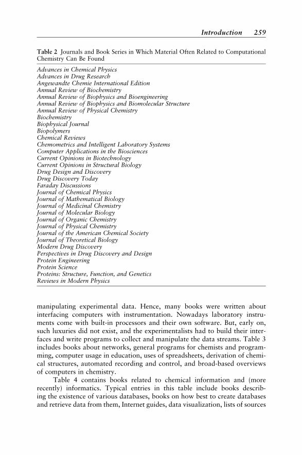
manipulating experimental data. Hence, many books were written aboutinterfacing computers with instrumentation. Nowadays laboratory instru-ments come with built-in processors and their own software. But, early on,such luxuries did not exist, and the experimentalists had to build their inter-faces and write programs to collect and manipulate the data streams. Table 3includes books about networks, general programs for chemists and program-ming, computer usage in education, uses of spreadsheets, derivation of chemi-cal structures, automated recording and control, and broad-based overviewsof computers in chemistry.

Table 4 contains books related to chemical information and (morerecently) informatics. Typical entries in this table include books describ-ing the existence of various databases, books on how best to create databasesand retrieve data from them, Internet guides, data visualization, lists of sources

Table 2 Journals and Book Series in Which Material Often Related to ComputationalChemistry Can Be Found

Advances in Chemical PhysicsAdvances in Drug ResearchAngewandte Chemie International EditionAnnual Review of BiochemistryAnnual Review of Biophysics and BioengineeringAnnual Review of Biophysics and Biomolecular StructureAnnual Review of Physical ChemistryBiochemistryBiophysical JournalBiopolymersChemical ReviewsChemometrics and Intelligent Laboratory SystemsComputer Applications in the BiosciencesCurrent Opinions in BiotechnologyCurrent Opinions in Structural BiologyDrug Design and DiscoveryDrug Discovery TodayFaraday DiscussionsJournal of Chemical PhysicsJournal of Mathematical BiologyJournal of Medicinal ChemistryJournal of Molecular BiologyJournal of Organic ChemistryJournal of Physical ChemistryJournal of the American Chemical SocietyJournal of Theoretical BiologyModern Drug DiscoveryPerspectives in Drug Discovery and DesignProtein EngineeringProtein ScienceProteins: Structure, Function, and GeneticsReviews in Modern Physics

Introduction 259

of chemical information, and so on. Some entries on bioinformatics, mathema-tical biology, genomics, and related topics are included because many compu-tational chemists are moving their research interests in those directions.

Table 5 lists general books including those with computational chemistryin their title. As we previously defined4 ‘‘computational chemistry’’, almost allof the books of this appendix could be suitably cataloged as books in compu-tational chemistry. However, the books in this table are more general thanmost of those in other tables. Hence, our Reviews in Computational Chemis-try series is listed here, as is the Encyclopedia of Computational Chemistry.Some of the entries in this table could have been placed in other tables, butbecause these books often cover several topics of computational chemistry,they are listed here.

Table 6 contains books on artificial intelligence and neural networks asrelated to chemistry. Also included are books on chemometrics. Table 7 is acompilation of computational chemistry books focused on pertinent areas ofphysical chemistry: crystallography, spectroscopy, and thermodynamics.

The next area of focus is quantum mechanics. Not surprisingly, this oldand well-studied field is represented by the greatest number of books in anysingle category. Rather than lump these 600 or so books together, we haveattempted to subdivide them. Accordingly, Table 8a lists textbooks and booksdescribing fundamental aspects of quantum mechanics. Many of these booksdeal with a high level of quantum theory. Table 8b contains books that aremore focused on applications of Hartree–Fock theory, density functional the-ory, and other electronic structure methods to relatively small molecular sys-tems. In some entries, clusters, solvated molecular systems, and the like areconsidered, but the emphasis is still on small molecules. In contrast, Table 8ccontains books focusing on larger systems. In particular, we have sorted outbooks treating mainly polymers, solids like crystals and metals, and othermaterials. Finally, Table 8d gives selected series and proceedings of quantumchemistry conferences and symposia, principally those that have been held ona long-term, regular basis. Examples of this are the ‘‘Sanibel meetings’’ and the‘‘Jerusalem conferences’’. Proceedings of other meetings like the NATO meet-ings on specialized subtopics of quantum mechanics have been distributedthroughout the above-mentioned tables dedicated to quantum chemistry.

Table 9 compiles books on molecular modeling. Again, this listing issomewhat arbitrary in the sense that many of these books could well havebeen placed in other categories. For instance, quantum mechanics is a wayof modeling molecules. Most of the books in this section contain the wordmodel or modeling in the title. Many of these books are broad in scope andcontain more than one aspect of modeling, whether it be quantum mechanics,molecular simulations, quantitative structure–activity relationships (QSAR),and so on.

Table 10 is a compilation of books related to molecular simulation. Thistable includes books on molecular mechanics, which is not a simulation

260 Books Published on the Topics of Computational Chemistry

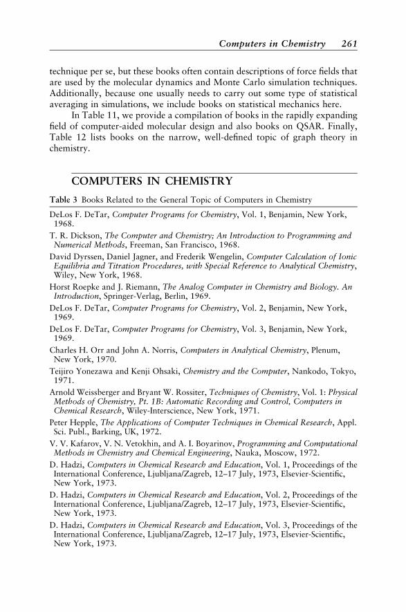
technique per se, but these books often contain descriptions of force fields thatare used by the molecular dynamics and Monte Carlo simulation techniques.Additionally, because one usually needs to carry out some type of statisticalaveraging in simulations, we include books on statistical mechanics here.

In Table 11, we provide a compilation of books in the rapidly expandingfield of computer-aided molecular design and also books on QSAR. Finally,Table 12 lists books on the narrow, well-defined topic of graph theory inchemistry.

COMPUTERS IN CHEMISTRY

Table 3 Books Related to the General Topic of Computers in Chemistry

DeLos F. DeTar, Computer Programs for Chemistry, Vol. 1, Benjamin, New York,1968.

T. R. Dickson, The Computer and Chemistry; An Introduction to Programming andNumerical Methods, Freeman, San Francisco, 1968.

David Dyrssen, Daniel Jagner, and Frederik Wengelin, Computer Calculation of IonicEquilibria and Titration Procedures, with Special Reference to Analytical Chemistry,Wiley, New York, 1968.

Horst Roepke and J. Riemann, The Analog Computer in Chemistry and Biology. AnIntroduction, Springer-Verlag, Berlin, 1969.

DeLos F. DeTar, Computer Programs for Chemistry, Vol. 2, Benjamin, New York,1969.

DeLos F. DeTar, Computer Programs for Chemistry, Vol. 3, Benjamin, New York,1969.

Charles H. Orr and John A. Norris, Computers in Analytical Chemistry, Plenum,New York, 1970.

Teijiro Yonezawa and Kenji Ohsaki, Chemistry and the Computer, Nankodo, Tokyo,1971.

Arnold Weissberger and Bryant W. Rossiter, Techniques of Chemistry, Vol. 1: PhysicalMethods of Chemistry, Pt. 1B: Automatic Recording and Control, Computers inChemical Research, Wiley-Interscience, New York, 1971.

Peter Hepple, The Applications of Computer Techniques in Chemical Research, Appl.Sci. Publ., Barking, UK, 1972.

V. V. Kafarov, V. N. Vetokhin, and A. I. Boyarinov, Programming and ComputationalMethods in Chemistry and Chemical Engineering, Nauka, Moscow, 1972.

D. Hadzi, Computers in Chemical Research and Education, Vol. 1, Proceedings of theInternational Conference, Ljubljana/Zagreb, 12–17 July, 1973, Elsevier-Scientific,New York, 1973.

D. Hadzi, Computers in Chemical Research and Education, Vol. 2, Proceedings of theInternational Conference, Ljubljana/Zagreb, 12–17 July, 1973, Elsevier-Scientific,New York, 1973.

D. Hadzi, Computers in Chemical Research and Education, Vol. 3, Proceedings of theInternational Conference, Ljubljana/Zagreb, 12–17 July, 1973, Elsevier-Scientific,New York, 1973.

Computers in Chemistry 261

Table 3 continued

Mircea Gheorghiu and Petru Filip, Application of Computers to Chemistry, Ed. Stiintif.,Bucharest, 1973.

S. P. Perone and D. K. Jones, Digital Computers in Scientific Instrumentation:Applications in Chemistry, McGraw-Hill, New York, 1973.

E. Ziegler, Computer in Analytical Chemistry, Akad. Verlagsgesellschaft, Frankfurt,1973.

P. S. Hunter, An Index to Computer-Produced Standard Interest Profiles in Chemistry,Applied Chemistry, Chemical Engineering, and Metallurgy, Sch. Librarianship,Polytech. North London, London, UK, 1973.

James S. Mattson, Harry B. Mark Jr., and Hubert C. MacDonald Jr., ComputerFundamentals for Chemists, Dekker, New York, 1973.

Ajit J. Thakkar, Computers in Chemistry, in Topics in Current Chemistry, Vol. 39,Springer, New York, 1973.

F. A. Brusentsev, Mathematical Methods of Solving Some Problems in Solid-StatePhysics and Structural Chemistry with Digital Computers, Nauk. Dumka, Kiev,1973.

James S. Mattson, Harry B. Mark Jr., and Hubert C. MacDonald Jr., Computer-AssistedInstruction in Chemistry, Part A: General Approach, Dekker, New York, 1974.

James S. Mattson, Harry B. Mark Jr., and Hubert C. MacDonald Jr., Computer-Assisted Instruction in Chemistry, Part B: Applications, Dekker, New York, 1974.

Yu. K. Shchipin and A. I. Novikov, Collection of Algorithms and Programs forOptimization Methods: Chemical Technology, Pt. 1: Nonlinear Programming, Mosk.Khim.-Tekhnol. Inst., Moscow, 1974.

V. N. Malkova, V. D. Ryzhkov, and V. I. Belevantsev, Study of Chemical Equilibriums(Calculation Methods, Algorithms, and Programs), Nauka, Sib. Otd., Novosibirsk,1974.

C. E. Klopfenstein and C. L. Wilkins, Computers in Chemical and BiochemicalResearch, Vol. 2, Academic Press, New York, 1974.

Charles L. Wilkins, Introduction to Computer Programming for Chemists. BasicVersion, Allyn & Bacon, Boston, 1974.

J. W. Frazer and F. W. Kunz, Computerized Laboratory Systems, in ASTM SpecialTechnical Publication, Vol. 578, ASTM, Philadelphia, 1975.

G. Beech, Fortran IV in Chemistry: An Introduction to Computer-Assisted Methods,Wiley, Chichester, 1975.

G. Beech, BASIC in Chemistry: A Self-Instructional Computing Course, Sigma Tech.Press, Wolverhampton, UK, 1975.

Julian S. May, Student Scientist Series: The Student Chemist Explores Computations,Richards Rosen, New York, 1975.

Leonard Soltzberg, BASIC and Chemistry, Houghton-Mifflin, Boston, 1975.

Peter Lykos, Computer Networking and Chemistry, in American Chemical SocietySymposium Series 19, American Chemical Society, Washington, DC, 1975.

Victor Marculetiu, Ligia Stoica, and Irina Constantinescu, Computations in Generaland Inorganic Chemistry, Editura Tehnica, Bucharest, 1976.

J. C. Simon, Computer Oriented Learning Processes, in NATO Advanced StudyInstitutes Series E: Applied Sciences, No. 14, Noordhoff, Leyden, Neth., 1976.

262 Books Published on the Topics of Computational Chemistry

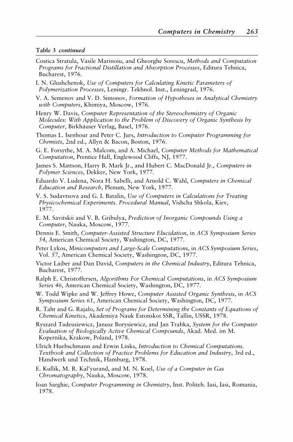
Table 3 continued

Costica Stratula, Vasile Marinoiu, and Gheorghe Sorescu, Methods and ComputationPrograms for Fractional Distillation and Absorption Processes, Editura Tehnica,Bucharest, 1976.

I. N. Glushchenok, Use of Computers for Calculating Kinetic Parameters ofPolymerization Processes, Leningr. Tekhnol. Inst., Leningrad, 1976.

V. A. Semenov and V. D. Simonov, Formation of Hypotheses in Analytical Chemistrywith Computers, Khimiya, Moscow, 1976.

Henry W. Davis, Computer Representation of the Stereochemistry of OrganicMolecules: With Application to the Problem of Discovery of Organic Synthesis byComputer, Birkhauser Verlag, Basel, 1976.

Thomas L. Isenhour and Peter C. Jurs, Introduction to Computer Programming forChemists, 2nd ed., Allyn & Bacon, Boston, 1976.

G. E. Forsythe, M. A. Malcom, and A. Michael, Computer Methods for MathematicalComputation, Prentice Hall, Englewood Cliffs, NJ, 1977.

James S. Mattson, Harry B. Mark Jr., and Hubert C. MacDonald Jr., Computers inPolymer Sciences, Dekker, New York, 1977.

Eduardo V. Ludena, Nora H. Sabelli, and Arnold C. Wahl, Computers in ChemicalEducation and Research, Plenum, New York, 1977.

V. S. Sudavtsova and G. I. Batalin, Use of Computers in Calculations for TreatingPhysicochemical Experiments. Procedural Manual, Vishcha Shkola, Kiev,1977.

E. M. Savitskii and V. B. Gribulya, Prediction of Inorganic Compounds Using aComputer, Nauka, Moscow, 1977.

Dennis E. Smith, Computer-Assisted Structure Elucidation, in ACS Symposium Series54, American Chemical Society, Washington, DC, 1977.

Peter Lykos, Minicomputers and Large-Scale Computations, in ACS Symposium Series,Vol. 57, American Chemical Society, Washington, DC, 1977.

Victor Laiber and Dan David, Computers in the Chemical Industry, Editura Tehnica,Bucharest, 1977.

Ralph E. Christoffersen, Algorithms For Chemical Computations, in ACS SymposiumSeries 46, American Chemical Society, Washington, DC, 1977.

W. Todd Wipke and W. Jeffrey Howe, Computer Assisted Organic Synthesis, in ACSSymposium Series 61, American Chemical Society, Washington, DC, 1977.

R. Taht and G. Rajalo, Set of Programs for Determining the Constants of Equations ofChemical Kinetics, Akademiya Nauk Estonskoi SSR, Tallin, USSR, 1978.

Ryszard Tadeusiewicz, Janusz Borysiewicz, and Jan Trabka, System for the ComputerEvaluation of Biologically Active Chemical Compounds, Akad. Med. im M.Kopernika, Krakow, Poland, 1978.

Ulrich Huebschmann and Erwin Links, Introduction to Chemical Computations.Textbook and Collection of Practice Problems for Education and Industry, 3rd ed.,Handwerk und Technik, Hamburg, 1978.

E. Kullik, M. R. Kal’yurand, and M. N. Koel, Use of a Computer in GasChromatography, Nauka, Moscow, 1978.

Ioan Sarghie, Computer Programming in Chemistry, Inst. Politeh. Iasi, Iasi, Romania,1978.

Computers in Chemistry 263

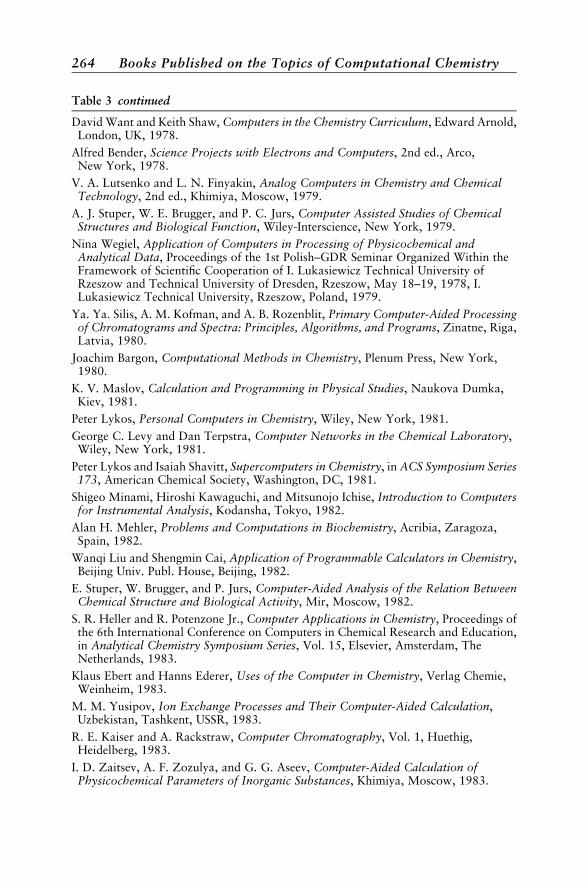
Table 3 continued

David Want and Keith Shaw, Computers in the Chemistry Curriculum, Edward Arnold,London, UK, 1978.

Alfred Bender, Science Projects with Electrons and Computers, 2nd ed., Arco,New York, 1978.

V. A. Lutsenko and L. N. Finyakin, Analog Computers in Chemistry and ChemicalTechnology, 2nd ed., Khimiya, Moscow, 1979.

A. J. Stuper, W. E. Brugger, and P. C. Jurs, Computer Assisted Studies of ChemicalStructures and Biological Function, Wiley-Interscience, New York, 1979.

Nina Wegiel, Application of Computers in Processing of Physicochemical andAnalytical Data, Proceedings of the 1st Polish–GDR Seminar Organized Within theFramework of Scientific Cooperation of I. Lukasiewicz Technical University ofRzeszow and Technical University of Dresden, Rzeszow, May 18–19, 1978, I.Lukasiewicz Technical University, Rzeszow, Poland, 1979.

Ya. Ya. Silis, A. M. Kofman, and A. B. Rozenblit, Primary Computer-Aided Processingof Chromatograms and Spectra: Principles, Algorithms, and Programs, Zinatne, Riga,Latvia, 1980.

Joachim Bargon, Computational Methods in Chemistry, Plenum Press, New York,1980.

K. V. Maslov, Calculation and Programming in Physical Studies, Naukova Dumka,Kiev, 1981.

Peter Lykos, Personal Computers in Chemistry, Wiley, New York, 1981.

George C. Levy and Dan Terpstra, Computer Networks in the Chemical Laboratory,Wiley, New York, 1981.

Peter Lykos and Isaiah Shavitt, Supercomputers in Chemistry, in ACS Symposium Series173, American Chemical Society, Washington, DC, 1981.

Shigeo Minami, Hiroshi Kawaguchi, and Mitsunojo Ichise, Introduction to Computersfor Instrumental Analysis, Kodansha, Tokyo, 1982.

Alan H. Mehler, Problems and Computations in Biochemistry, Acribia, Zaragoza,Spain, 1982.

Wanqi Liu and Shengmin Cai, Application of Programmable Calculators in Chemistry,Beijing Univ. Publ. House, Beijing, 1982.

E. Stuper, W. Brugger, and P. Jurs, Computer-Aided Analysis of the Relation BetweenChemical Structure and Biological Activity, Mir, Moscow, 1982.

S. R. Heller and R. Potenzone Jr., Computer Applications in Chemistry, Proceedings ofthe 6th International Conference on Computers in Chemical Research and Education,in Analytical Chemistry Symposium Series, Vol. 15, Elsevier, Amsterdam, TheNetherlands, 1983.

Klaus Ebert and Hanns Ederer, Uses of the Computer in Chemistry, Verlag Chemie,Weinheim, 1983.

M. M. Yusipov, Ion Exchange Processes and Their Computer-Aided Calculation,Uzbekistan, Tashkent, USSR, 1983.

R. E. Kaiser and A. Rackstraw, Computer Chromatography, Vol. 1, Huethig,Heidelberg, 1983.

I. D. Zaitsev, A. F. Zozulya, and G. G. Aseev, Computer-Aided Calculation ofPhysicochemical Parameters of Inorganic Substances, Khimiya, Moscow, 1983.

264 Books Published on the Topics of Computational Chemistry

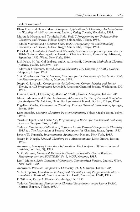
Table 3 continued

Klaus Ebert and Hanns Ederer, Computer Applications in Chemistry. An Introductionto Working with Microcomputers, 2nd ed., Verlag Chemie, Weinheim, 1984.

Murotada Hazama and Yoshitaka Sudo, BASIC Programming for UnderstandingChemistry and Physics, Nikkan Kogyo Shinbunsha, Tokyo, 1984.

Tadashi Mamuro and Yoshitaka Sudo, BASIC Programing for UnderstandingChemistry and Physics, Nikkan Kogyo Shinbunsha, Tokyo, 1984.

Peter Lykos, Computer Education of Chemists, Based on a symposium presented at the184th National Meeting of the American Chemical Society, Kansas City, Missouri,September 1982, Wiley, New York, 1984.

L. S. Polak, M. Ya. Gol’denberg, and A. A. Levitskii, Computing Methods in ChemicalKinetics, Nauka, Moscow, 1984.

Tadayoshi Yoshimura, Introduction to Chemistry Dry Lab Using BASIC, KyoritsuShuppan, Tokyo, 1984.

S. A. Vorob’ev and Yu. V. Shvarov, Programs for the Processing of Geochemical Dataon Microcomputers, Nedra, Moscow, 1984.

Joseph G. Liscouski, Computers in the Laboratory: Current Practice and FutureTrends, in ACS Symposium Series 265, American Chemical Society, Washington, DC,1984.

Osamu Kikuchi, Chemistry by Means of BASIC, Kyoritsu Shuppan, Tokyo, 1984.

Masato Mamiya and Toshio Nishikawa, Advances in the Use of Personal Computersfor Analytical Technicians, Nihon Kankyo Sokutai Bunseki Kyokai, Tokyo, 1984.

Engelbert Ziegler, Computers in Chemistry. Practice Oriented Introduction, Springer,Berlin, 1984.

Kozo Inuzuka, Learning Chemistry by Microcomputers, Tokyo Kagaku Dojin, Tokyo,1984.

Yukihiro Eguchi and Yoichi Aso, Programming in BASIC for Biochemical Problems,Kyoritsu Shuppan, Tokyo, 1985.

Tadayosi Yoshimura, Collection of Software for the Personal Computer in Chemistry.1985 ed., The Association of Personal Computer for Chemists, Sabae, Japan, 1985.

Robert W. Numrich, Supercomputer Applications, Plenum, New York, 1985.

Joseph H. Noggle, Physical Chemistry on a Microcomputer, Little, Brown, Boston,1985.

Anonymus, Managing Laboratory Information: The Computer Options, TechnicalInsights, Fort Lee, NJ, 1985.

V. K. Matveev, Numerical Methods in Chemistry: Scientific Course Based onMicrocomputers and FORTRAN, Pt. 1, MGU, Moscow, 1985.

Leo J. Malone, Basic Concepts of Chemistry, Computerized Version, 2nd ed., Wiley,New York, 1985.

Anonymus, Personal Computers in Chemistry, Pt. 1, Maruzen, Tokyo, 1985.

V. A. Kropotov, Calculations in Analytical Chemistry Using Programmable Micro-calculators: Textbook, Simferopolskii Gos. Un-T., Simferopol, USSR, 1985.

P. Williams, Enzpack, Elsevier, Cambridge, UK, 1985.

Tadayosi Yoshimura, Simulation of Chemical Experiments by the Use of BASIC,Koritsu Shuppan, Tokyo, 1985.

Computers in Chemistry 265

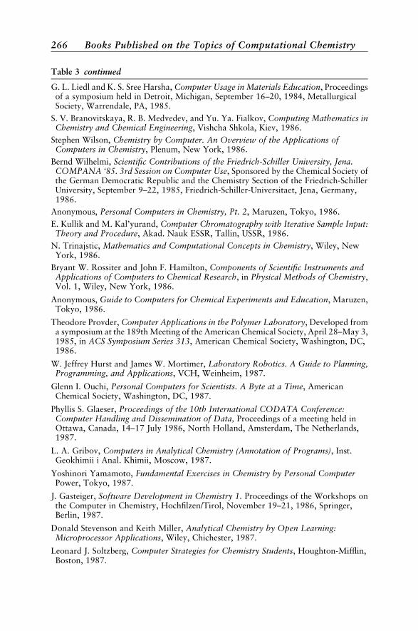
Table 3 continued

G. L. Liedl and K. S. Sree Harsha, Computer Usage in Materials Education, Proceedingsof a symposium held in Detroit, Michigan, September 16–20, 1984, MetallurgicalSociety, Warrendale, PA, 1985.

S. V. Branovitskaya, R. B. Medvedev, and Yu. Ya. Fialkov, Computing Mathematics inChemistry and Chemical Engineering, Vishcha Shkola, Kiev, 1986.

Stephen Wilson, Chemistry by Computer. An Overview of the Applications ofComputers in Chemistry, Plenum, New York, 1986.

Bernd Wilhelmi, Scientific Contributions of the Friedrich-Schiller University, Jena.COMPANA ‘85. 3rd Session on Computer Use, Sponsored by the Chemical Society ofthe German Democratic Republic and the Chemistry Section of the Friedrich-SchillerUniversity, September 9–22, 1985, Friedrich-Schiller-Universitaet, Jena, Germany,1986.

Anonymous, Personal Computers in Chemistry, Pt. 2, Maruzen, Tokyo, 1986.

E. Kullik and M. Kal’yurand, Computer Chromatography with Iterative Sample Input:Theory and Procedure, Akad. Nauk ESSR, Tallin, USSR, 1986.

N. Trinajstic, Mathematics and Computational Concepts in Chemistry, Wiley, NewYork, 1986.

Bryant W. Rossiter and John F. Hamilton, Components of Scientific Instruments andApplications of Computers to Chemical Research, in Physical Methods of Chemistry,Vol. 1, Wiley, New York, 1986.

Anonymous, Guide to Computers for Chemical Experiments and Education, Maruzen,Tokyo, 1986.

Theodore Provder, Computer Applications in the Polymer Laboratory, Developed froma symposium at the 189th Meeting of the American Chemical Society, April 28–May 3,1985, in ACS Symposium Series 313, American Chemical Society, Washington, DC,1986.

W. Jeffrey Hurst and James W. Mortimer, Laboratory Robotics. A Guide to Planning,Programming, and Applications, VCH, Weinheim, 1987.

Glenn I. Ouchi, Personal Computers for Scientists. A Byte at a Time, AmericanChemical Society, Washington, DC, 1987.

Phyllis S. Glaeser, Proceedings of the 10th International CODATA Conference:Computer Handling and Dissemination of Data, Proceedings of a meeting held inOttawa, Canada, 14–17 July 1986, North Holland, Amsterdam, The Netherlands,1987.

L. A. Gribov, Computers in Analytical Chemistry (Annotation of Programs), Inst.Geokhimii i Anal. Khimii, Moscow, 1987.

Yoshinori Yamamoto, Fundamental Exercises in Chemistry by Personal ComputerPower, Tokyo, 1987.

J. Gasteiger, Software Development in Chemistry 1. Proceedings of the Workshops onthe Computer in Chemistry, Hochfilzen/Tirol, November 19–21, 1986, Springer,Berlin, 1987.

Donald Stevenson and Keith Miller, Analytical Chemistry by Open Learning:Microprocessor Applications, Wiley, Chichester, 1987.

Leonard J. Soltzberg, Computer Strategies for Chemistry Students, Houghton-Mifflin,Boston, 1987.

266 Books Published on the Topics of Computational Chemistry

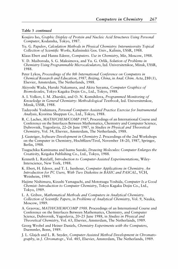
Table 3 continued

Koujiro Iso, Graphic Display of Protein and Nucleic Acid Structures Using PersonalComputer, Kodansha, Tokyo, 1987.

Yu. G. Papulov, Calculation Methods in Physical Chemistry: Interuniversity TopicalCollection of Scientific Works, Kalininskii Gos. Univ., Kalinin, USSR, 1988.

Klaus Ebert and Hanns Ederer, Computers. Use in Chemistry, Mir, Moscow, 1988.

V. D. Maiboroda, S. G. Maksimova, and Yu. G. Orlik, Solution of Problems inChemistry Using Programmable Microcalculators, Izd. Universitetskoe, Minsk, USSR,1988.

Peter Lykos, Proceedings of the 8th International Conference on Computers inChemical Research and Education, 1987, Beijing, China, in Anal. Chim. Acta, 210 (1),Elsevier, Amsterdam, The Netherlands, 1988.

Akiyoshi Wada, Haruki Nakamura, and Akira Suyama, Computer Graphics ofBiomolecules, Tokyo Kagaku Dojin Co., Ltd., Tokyo, 1988.

A. I. Volkov, I. M. Zharskii, and O. N. Komshilova, Programmed Monitoring ofKnowledge in General Chemistry: Methodological Textbook, Izd. Universitetskoe,Minsk, USSR, 1988.

Tadayoshi Yoshimura, Personal Computer-Assisted Practice Exercise for InstrumentalAnalysis, Kyoritsu Shuppan Co., Ltd., Tokyo, 1988.

R. C. Lacher, MATH/CHEM/COMP 1987, Proceedings of an International Course andConference on the Interfaces Between Mathematics, Chemistry and Computer Science,Dubrovnik, Yugoslavia, 22–26 June 1987, in Studies in Physical and TheoreticalChemistry, Vol. 54, Elsevier, Amsterdam, The Netherlands, 1988.

J. Gasteiger, Software Development in Chemistry 2. Proceedings of the 2nd Workshopson the Computer in Chemistry, Hochfilzen/Tirol, November 18–20, 1987, Springer,Berlin, 1988.

Tsuguchika Kaminuma and Isamu Suzuki, Drawing Molecules: Computer Enlarges theCreativity, Keigaku Publishing Co., Ltd., Tokyo, 1988.

Kenneth L. Ratzlaff, Introduction to Computer-Assisted Experimentations, Wiley-Interscience, New York, 1988.

K. Ebert, H. Ederer, and T. L. Isenhour, Computer Applications in Chemistry. AnIntroduction for PC Users, With Two Diskettes in BASIC and PASCAL, VCH,Weinheim, 1989.

Hajime Nishimura, Kizashi Yamaguchi, and Mototsugu Yoshida, Computer Is a GoodChemist: Introduction to Computer Chemistry, Tokyo Kagaku Dojin Co., Ltd.,Tokyo, 1989.

L. A. Gribov, Mathematical Methods and Computers in Analytical Chemistry.Collection of Scientific Papers, in Problems of Analytical Chemistry, Vol. 9, Nauka,Moscow, 1989.

A. Graovac, MATH/CHEM/COMP 1988. Proceedings of an International Course andConference on the Interfaces Between Mathematics, Chemistry, and ComputerScience, Dubrovnik, Yugoslavia, 20–25 June 1988, in Studies in Physical andTheoretical Chemistry, Vol. 63, Elsevier, Amsterdam, The Netherlands, 1989.

Georg Wrobel and Heiner Daniels, Chemistry Experiments with the Computers,Duemmler, Bonn, 1989.

J. L. Glajch and L. R. Snyder, Computer-Assisted Method Development in Chromato-graphy, in J. Chromatogr., Vol. 485, Elsevier, Amsterdam, The Netherlands, 1989.

Computers in Chemistry 267

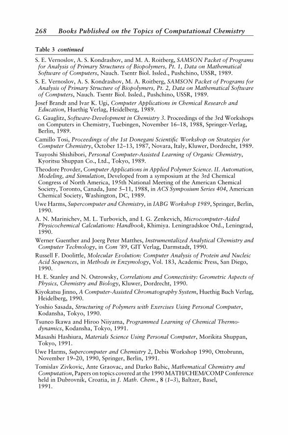
Table 3 continued

S. E. Vernoslov, A. S. Kondrashov, and M. A. Roitberg, SAMSON Packet of Programsfor Analysis of Primary Structures of Biopolymers, Pt. 1, Data on MathematicalSoftware of Computers, Nauch. Tsentr Biol. Issled., Pushchino, USSR, 1989.

S. E. Vernoslov, A. S. Kondrashov, M. A. Roitberg, SAMSON Packet of Programs forAnalysis of Primary Structure of Biopolymers, Pt. 2, Data on Mathematical Softwareof Computers, Nauch. Tsentr Biol. Issled., Pushchino, USSR, 1989.

Josef Brandt and Ivar K. Ugi, Computer Applications in Chemical Research andEducation, Huethig Verlag, Heidelberg, 1989.

G. Gauglitz, Software-Development in Chemistry 3. Proceedings of the 3rd Workshopson Computers in Chemistry, Tuebingen, November 16–18, 1988, Springer-Verlag,Berlin, 1989.

Camillo Tosi, Proceedings of the 1st Donegani Scientific Workshop on Strategies forComputer Chemistry, October 12–13, 1987, Novara, Italy, Kluwer, Dordrecht, 1989.

Tsuyoshi Shishibori, Personal Computer-Assisted Learning of Organic Chemistry,Kyoritsu Shuppan Co., Ltd., Tokyo, 1989.

Theodore Provder, Computer Applications in Applied Polymer Science. II. Automation,Modeling, and Simulation, Developed from a symposium at the 3rd ChemicalCongress of North America, 195th National Meeting of the American ChemicalSociety, Toronto, Canada, June 5–11, 1988, in ACS Symposium Series 404, AmericanChemical Society, Washington, DC, 1989.

Uwe Harms, Supercomputer and Chemistry, in IABG Workshop 1989, Springer, Berlin,1990.

A. N. Marinichev, M. L. Turbovich, and I. G. Zenkevich, Microcomputer-AidedPhysicochemical Calculations: Handbook, Khimiya. Leningradskoe Otd., Leningrad,1990.

Werner Guenther and Joerg Peter Matthes, Instrumentalized Analytical Chemistry andComputer Technology, in Com ’89, GIT Verlag, Darmstadt, 1990.

Russell F. Doolittle, Molecular Evolution: Computer Analysis of Protein and NucleicAcid Sequences, in Methods in Enzymology, Vol. 183, Academic Press, San Diego,1990.

H. E. Stanley and N. Ostrowsky, Correlations and Connectivity: Geometric Aspects ofPhysics, Chemistry and Biology, Kluwer, Dordrecht, 1990.

Kiyokatsu Jinno, A Computer-Assisted Chromatography System, Huethig Buch Verlag,Heidelberg, 1990.

Yoshio Sasada, Structuring of Polymers with Exercises Using Personal Computer,Kodansha, Tokyo, 1990.

Tsuneo Ikawa and Hiroo Niiyama, Programmed Learning of Chemical Thermo-dynamics, Kodansha, Tokyo, 1991.

Masashi Hashiura, Materials Science Using Personal Computer, Morikita Shuppan,Tokyo, 1991.

Uwe Harms, Supercomputer and Chemistry 2, Debis Workshop 1990, Ottobrunn,November 19–20, 1990, Springer, Berlin, 1991.

Tomislav Zivkovic, Ante Graovac, and Darko Babic, Mathematical Chemistry andComputation, Papers on topics covered at the 1990 MATH/CHEM/COMP Conferenceheld in Dubrovnik, Croatia, in J. Math. Chem., 8 (1–3), Baltzer, Basel,1991.

268 Books Published on the Topics of Computational Chemistry

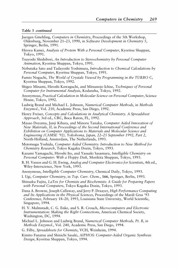
Table 3 continued

Juergen Gmehling, Computers in Chemistry, Proceedings of the 5th Workshop,Oldenburg, November 21–23, 1990, in Software Development in Chemistry 5,Springer, Berlin, 1991.

Hiroya Kamei, Analysis of Protein With a Personal Computer, Kyoritsu Shuppan,Tokyo, 1991.

Tsuyoshi Shishibori, An Introduction to Stereochemistry by Personal ComputerAnimation, Kyoritsu Shuppan, Tokyo, 1991.

Nobutaka Sato and Tadayoshi Yoshimura, Introduction to Chemical Calculations byPersonal Computer, Kyoritsu Shuppan, Tokyo, 1991.

Fumio Noguchi, The World of Crystals Viewed by Programming in the TURBO C,Kyoritsu Shuppan, Tokyo, 1992.

Shigeo Minami, Hiroshi Kawaguchi, and Mitsunojo Ichise, Techniques of PersonalComputer for Instrumental Analysis, Kodansha, Tokyo, 1992.

Anonymous, Practical Calculation in Molecular Science on Personal Computer, ScienceHouse, Tokyo, 1992.

Ludwig Brand and Michael L. Johnson, Numerical Computer Methods, in MethodsEnzymol., Vol. 210, Academic Press, San Diego, 1992.

Henry Freiser, Concepts and Calculations in Analytical Chemistry. A SpreadsheetApproach, 3rd ed., CRC, Boca Raton, FL, 1992.

Masao Doyama, Junji Kihara, and Minoru Tanaka, Computer Aided Innovation ofNew Materials, II, in Proceedings of the Second International Conference andExhibition on Computer Applications to Materials and Molecular Science andEngineering (CAMSE ’92), Yokohoma, Japan, 22–25 September 1992, Part 2,North-Holland, Amsterdam, The Netherlands, 1993.

Mototsugu Yoshida, Computer Aided Chemistry: Introduction to New Method forChemistry Research, Tokyo Kagaku Dozin, Tokyo, 1993.

Kazumi Yamaguchi, Hiroshi Ito, and Yasuaki Sasamura, Intelligible Chemistry onPersonal Computer: With a Floppy Disk, Morikita Shuppan, Tokyo, 1993.

B. H. Vassos and G. H. Ewing, Analog and Computer Electronics for Scientists, 4th ed.,Wiley-Interscience, New York, 1993.

Anonymous, Intelligible Computer Chemistry, Chemical Daily, Tokyo, 1993.

I. Ugi, Computer Chemistry, in Top. Curr. Chem., 166, Springer, Berlin, 1993.

Shinsaku Fujita, LaTex for Chemists and Biochemists: A Guide for Preparing Paperswith Personal Computers, Tokyo Kagaku Dozin, Tokyo, 1993.

Dana A. Browne, Joseph Callaway, and Jerry P. Draayer, High Performance Computingand Its Applications in the Physical Sciences, Proceedings of the Mardi Gras ‘93Conference, February 18–20, 1993, Louisiana State University, World Scientific,Singapore, 1994.

H. V. Malmstadt, C. G. Enke, and S. R. Crouch, Microcomputers and ElectronicInstrumentation: Making the Right Connections, American Chemical Society,Washington, DC, 1994.

Michael L. Johnson and Ludwig Brand, Numerical Computer Methods, Pt. B, inMethods Enzymol., Vol. 240, Academic Press, San Diego, 1994.

G. Filby, Spreadsheets for Chemists, VCH, Weinheim, 1994.

Kimito Funatsu and Shinichi Sasaki, AIPHOS: Computer-Aided Organic SynthesisDesign, Kyoritsu Shuppan, Tokyo, 1994.

Computers in Chemistry 269

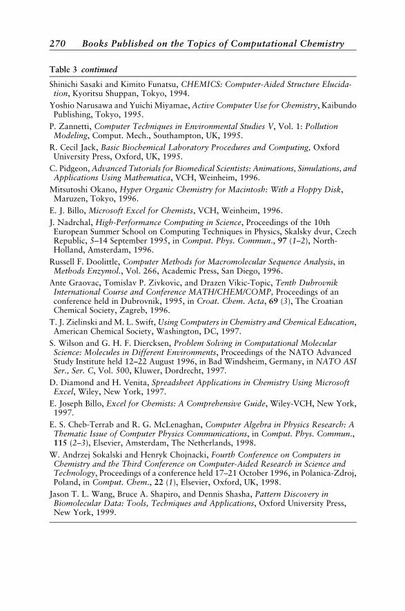
Table 3 continued

Shinichi Sasaki and Kimito Funatsu, CHEMICS: Computer-Aided Structure Elucida-tion, Kyoritsu Shuppan, Tokyo, 1994.

Yoshio Narusawa and Yuichi Miyamae, Active Computer Use for Chemistry, KaibundoPublishing, Tokyo, 1995.

P. Zannetti, Computer Techniques in Environmental Studies V, Vol. 1: PollutionModeling, Comput. Mech., Southampton, UK, 1995.

R. Cecil Jack, Basic Biochemical Laboratory Procedures and Computing, OxfordUniversity Press, Oxford, UK, 1995.

C. Pidgeon, Advanced Tutorials for Biomedical Scientists: Animations, Simulations, andApplications Using Mathematica, VCH, Weinheim, 1996.

Mitsutoshi Okano, Hyper Organic Chemistry for Macintosh: With a Floppy Disk,Maruzen, Tokyo, 1996.

E. J. Billo, Microsoft Excel for Chemists, VCH, Weinheim, 1996.

J. Nadrchal, High-Performance Computing in Science, Proceedings of the 10thEuropean Summer School on Computing Techniques in Physics, Skalsky dvur, CzechRepublic, 5–14 September 1995, in Comput. Phys. Commun., 97 (1–2), North-Holland, Amsterdam, 1996.

Russell F. Doolittle, Computer Methods for Macromolecular Sequence Analysis, inMethods Enzymol., Vol. 266, Academic Press, San Diego, 1996.

Ante Graovac, Tomislav P. Zivkovic, and Drazen Vikic-Topic, Tenth DubrovnikInternational Course and Conference MATH/CHEM/COMP, Proceedings of anconference held in Dubrovnik, 1995, in Croat. Chem. Acta, 69 (3), The CroatianChemical Society, Zagreb, 1996.

T. J. Zielinski and M. L. Swift, Using Computers in Chemistry and Chemical Education,American Chemical Society, Washington, DC, 1997.

S. Wilson and G. H. F. Diercksen, Problem Solving in Computational MolecularScience: Molecules in Different Environments, Proceedings of the NATO AdvancedStudy Institute held 12–22 August 1996, in Bad Windsheim, Germany, in NATO ASISer., Ser. C, Vol. 500, Kluwer, Dordrecht, 1997.

D. Diamond and H. Venita, Spreadsheet Applications in Chemistry Using MicrosoftExcel, Wiley, New York, 1997.

E. Joseph Billo, Excel for Chemists: A Comprehensive Guide, Wiley-VCH, New York,1997.

E. S. Cheb-Terrab and R. G. McLenaghan, Computer Algebra in Physics Research: AThematic Issue of Computer Physics Communications, in Comput. Phys. Commun.,115 (2–3), Elsevier, Amsterdam, The Netherlands, 1998.

W. Andrzej Sokalski and Henryk Chojnacki, Fourth Conference on Computers inChemistry and the Third Conference on Computer-Aided Research in Science andTechnology, Proceedings of a conference held 17–21 October 1996, in Polanica-Zdroj,Poland, in Comput. Chem., 22 (1), Elsevier, Oxford, UK, 1998.

Jason T. L. Wang, Bruce A. Shapiro, and Dennis Shasha, Pattern Discovery inBiomolecular Data: Tools, Techniques and Applications, Oxford University Press,New York, 1999.

270 Books Published on the Topics of Computational Chemistry

CHEMICAL INFORMATION

Table 4 Books on Chemical Information

Carlos A. Cuadra, Annual Review of Information Science and Technology, Vol. 2,Interscience, New York, 1967.

Carlos A. Cuadra, Annual Review of Information Science and Technology, Vol. 3,Encyclopedia Britannica, Chicago, 1968.

M. Fiskus, Construction of an Enzymology Data Bank for Real-Time Computer UseCNRS, Paris, 1969.

Bernard Houghton, Computer Based Information Retrieval Systems, Archon, Hamden,CT, 1969.

R. T. Bottle, The Use of Chemical Literature (Information Sources for Research andDevelopment), 2nd ed., Butterworth, London, UK, 1969.

Anthony P. Harvey, Directory of Scientific Directories. A World Guide to ScientificDirectories Including Medicine, Agriculture, Engineering, Manufacturing, andIndustrial Directories, Hodgson, Guernsey, Channel Islands, UK, 1969.

Saul Herner, A Brief Guide to Sources of Scientific and Technical Information,Information Resources Press, Washington, DC, 1970.

H. Evers, Computer-Based Chemical Information, Royal Netherlands ChemicalSociety, Hague, The Netherlands, 1970.

Gerald Jahoda, Information Storage and Retrieval Systems for Individual Researchers,Wiley-Interscience, New York, 1970.

Carlos A. Cuadra and Ann W. Luke, Annual Review of Information Science andTechnology, Vol. 5, Encyclopedia Britannica, Chicago, 1970.

Michael Lynch, Judith M. Harrison, and William G. Town, Computer Handling ofChemical Structure Information, Elsevier, New York, 1971.

E. L. Gefter, Methods of Working with the Chemical Literature, Khimiya, Moscow,1972.

A. A. Belaya, Theory and Practice of Scientific Information in the Field of Chemistry.Collection of Abstracts 1963–1969, Nauk. Dumka, Kiev, 1972.

Edward M. Arnett and Allen Kent, Computer-Based Chemical Information, Dekker,New York, 1973.

Y. S. Touloukian, Thermophysical Properties Research Literature Retrieval Guide,Suppl. 1: 1964–1970, Vol. 3: Alloys, Intermetallic Compounds, and Cermets, Plenum,New York, 1973.

A. I. Chernyi, Introduction to Information Retrieval Theory, Lectures presented at theCourse for Information Officers and Documentalists from Developing Countries heldby VINITI, 4 September–16 November, 1973, Vses. Inst. Nauchn. Tekhn. Inform.,Moscow, 1973.

Marian Lescinsky, Recording of Information on Organic Materials, Academia, Prague,1974.

G. E. Vleduts and E. A. Geivandov, Automated Information Systems for Chemistry,Nauka, Moscow, 1974.

W. T. Wipke, S. R. Heller, and R. J. Feldmann, Computer Representation andManipulation of Chemical Information, Kreiger, New York, 1974.

Chemical Information 271

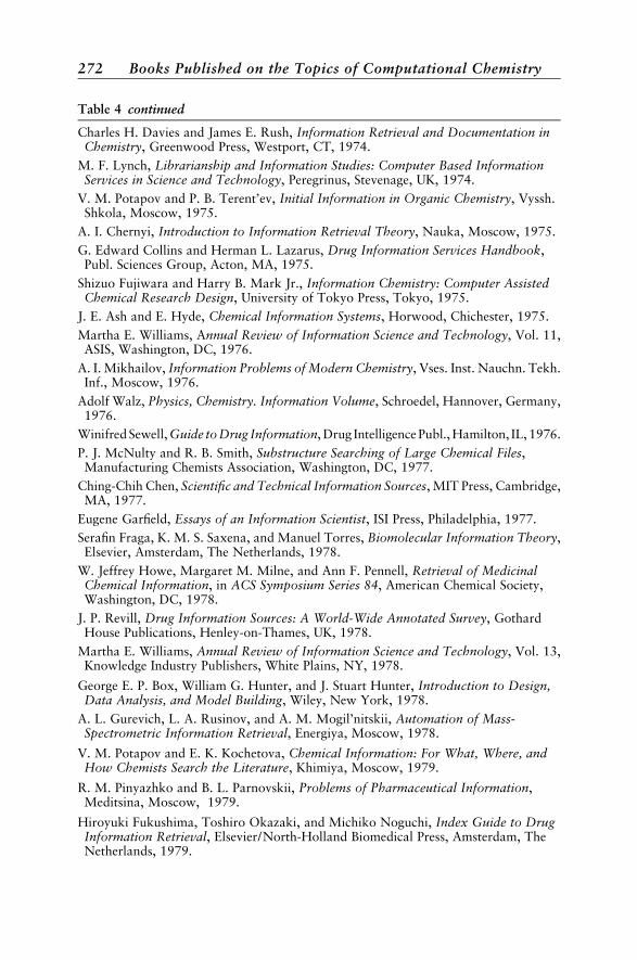
Table 4 continued

Charles H. Davies and James E. Rush, Information Retrieval and Documentation inChemistry, Greenwood Press, Westport, CT, 1974.

M. F. Lynch, Librarianship and Information Studies: Computer Based InformationServices in Science and Technology, Peregrinus, Stevenage, UK, 1974.

V. M. Potapov and P. B. Terent’ev, Initial Information in Organic Chemistry, Vyssh.Shkola, Moscow, 1975.

A. I. Chernyi, Introduction to Information Retrieval Theory, Nauka, Moscow, 1975.

G. Edward Collins and Herman L. Lazarus, Drug Information Services Handbook,Publ. Sciences Group, Acton, MA, 1975.

Shizuo Fujiwara and Harry B. Mark Jr., Information Chemistry: Computer AssistedChemical Research Design, University of Tokyo Press, Tokyo, 1975.

J. E. Ash and E. Hyde, Chemical Information Systems, Horwood, Chichester, 1975.

Martha E. Williams, Annual Review of Information Science and Technology, Vol. 11,ASIS, Washington, DC, 1976.

A. I. Mikhailov, Information Problems of Modern Chemistry, Vses. Inst. Nauchn. Tekh.Inf., Moscow, 1976.

Adolf Walz, Physics, Chemistry. Information Volume, Schroedel, Hannover, Germany,1976.

Winifred Sewell,Guide to Drug Information, Drug IntelligencePubl., Hamilton, IL, 1976.

P. J. McNulty and R. B. Smith, Substructure Searching of Large Chemical Files,Manufacturing Chemists Association, Washington, DC, 1977.

Ching-Chih Chen, Scientific and Technical Information Sources, MIT Press, Cambridge,MA, 1977.

Eugene Garfield, Essays of an Information Scientist, ISI Press, Philadelphia, 1977.

Serafin Fraga, K. M. S. Saxena, and Manuel Torres, Biomolecular Information Theory,Elsevier, Amsterdam, The Netherlands, 1978.

W. Jeffrey Howe, Margaret M. Milne, and Ann F. Pennell, Retrieval of MedicinalChemical Information, in ACS Symposium Series 84, American Chemical Society,Washington, DC, 1978.

J. P. Revill, Drug Information Sources: A World-Wide Annotated Survey, GothardHouse Publications, Henley-on-Thames, UK, 1978.

Martha E. Williams, Annual Review of Information Science and Technology, Vol. 13,Knowledge Industry Publishers, White Plains, NY, 1978.

George E. P. Box, William G. Hunter, and J. Stuart Hunter, Introduction to Design,Data Analysis, and Model Building, Wiley, New York, 1978.

A. L. Gurevich, L. A. Rusinov, and A. M. Mogil’nitskii, Automation of Mass-Spectrometric Information Retrieval, Energiya, Moscow, 1978.

V. M. Potapov and E. K. Kochetova, Chemical Information: For What, Where, andHow Chemists Search the Literature, Khimiya, Moscow, 1979.

R. M. Pinyazhko and B. L. Parnovskii, Problems of Pharmaceutical Information,Meditsina, Moscow, 1979.

Hiroyuki Fukushima, Toshiro Okazaki, and Michiko Noguchi, Index Guide to DrugInformation Retrieval, Elsevier/North-Holland Biomedical Press, Amsterdam, TheNetherlands, 1979.

272 Books Published on the Topics of Computational Chemistry

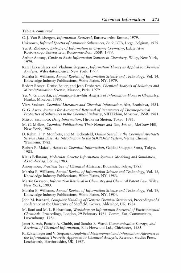
Table 4 continued

C. J. Van Rijsbergen, Information Retrieval, Butterworths, Boston, 1979.

Unknown, Infrared Spectra of Antibiotic Substances, Pt. 9, ICIA, Liege, Belgium, 1979.

Yu. A. Zhdanov, Entropy of Information in Organic Chemistry, Izdatel’stvoRostovskogo Universiteta, Rostov-on-Don, USSR, 1979.

Arthur Antony, Guide to Basic Information Sources in Chemistry, Wiley, New York,1979.

Karel Eckschlager and Vladimir Stepanek, Information Theory as Applied to ChemicalAnalysis, Wiley-Interscience, New York, 1979.

Martha E. Williams, Annual Review of Information Science and Technology, Vol. 14,Knowledge Industry Publications, White Plains, NY, 1979.

Robert Rosset, Denise Bauer, and Jean Desbarres, Chemical Analysis of Solutions andMicroinformation Science, Masson, Paris, 1979.

Yu. V. Granovskii, Information-Scientific Analysis of Information Flows in Chemistry,Nauka, Moscow, 1980.

Viera Saskova, Chemical Literature and Chemical Information, Alfa, Bratislava, 1981.

G. G. Aseev, Systems for Automated Retrieval of Parameters of ThermophysicalProperties of Substances in the Chemical Industry, NIITEkhim, Moscow, USSR, 1981.

Mitsuo Sasamoto, Drug Information, Hirokawa Shoten, Tokyo, 1981.

M. G. Mellon, Chemical Publications: Their Nature and Use, 5th ed., McGraw-Hill,New York, 1982.

D. Rehm, F. P. Monforts, and M. Ockenfeld, Online Search in the Chemical AbstractsService Data Base. An Introduction to the SDC/Orbit System, Verlag Chemie,Weinheim, 1982.

Robert E. Maizell, Access to Chemical Information, Gakkai Shuppan Senta, Tokyo,1983.

Klaus Bellmann, Molecular Genetic Information Systems: Modeling and Simulation,Akad.-Verlag, Berlin, 1983.

Anonymous, Practical Use of Chemical Abstracts, Kodansha, Tokyo, 1983.

Martha E. Williams, Annual Review of Information Science and Technology, Vol. 18,Knowledge Industry Publications, White Plains, NY, 1983.

Martin Grayson, Information Retrieval in Chemistry and Chemical Patent Law, Wiley,New York, 1983.

Martha E. Williams, Annual Review of Information Science and Technology, Vol. 19,Knowledge Industry Publications, White Plains, NY, 1984.

John M. Barnard, Computer Handling of Generic Chemical Structures, Proceedings of aconference at the University of Sheffield, Gower, Aldershot, UK, 1984.

M. Boni and M. L. Richardson, Workshop on Information Retrieval of EnvironmentalChemicals. Proceedings, London, 29 February 1984, Comm. Eur. Communities,Luxembourg, 1984.

Janet E. Ash, Pamela A. Chubb, and Sandra E. Ward, Communication Storage, andRetrieval of Chemical Information, Ellis Horwood Ltd., Chichester, 1985.

K. Eckschlager and V. Stepanek, Analytical Measurement and Information: Advances inthe Information Theoretic Approach to Chemical Analysis, Research Studies Press,Letchworth, Hertfordshire, UK, 1985.

Chemical Information 273

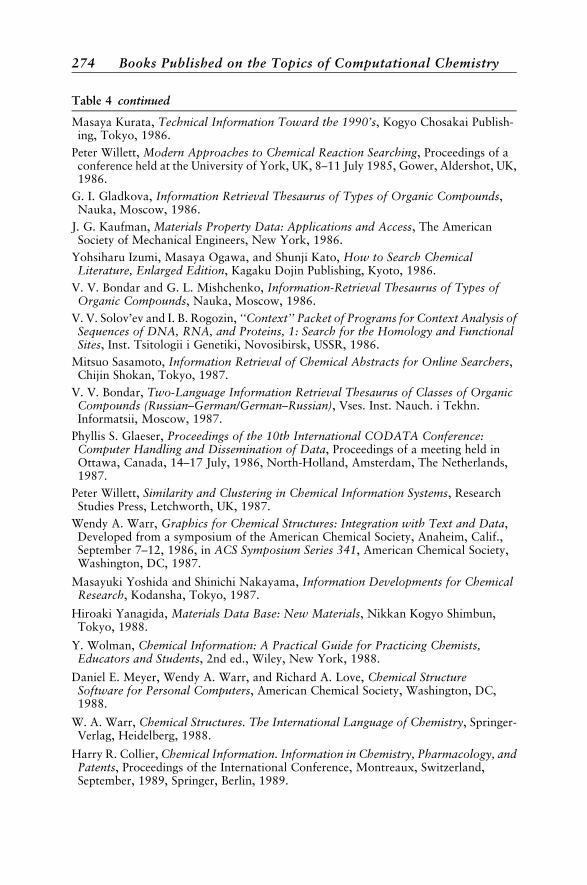
Table 4 continued

Masaya Kurata, Technical Information Toward the 1990’s, Kogyo Chosakai Publish-ing, Tokyo, 1986.

Peter Willett, Modern Approaches to Chemical Reaction Searching, Proceedings of aconference held at the University of York, UK, 8–11 July 1985, Gower, Aldershot, UK,1986.

G. I. Gladkova, Information Retrieval Thesaurus of Types of Organic Compounds,Nauka, Moscow, 1986.

J. G. Kaufman, Materials Property Data: Applications and Access, The AmericanSociety of Mechanical Engineers, New York, 1986.

Yohsiharu Izumi, Masaya Ogawa, and Shunji Kato, How to Search ChemicalLiterature, Enlarged Edition, Kagaku Dojin Publishing, Kyoto, 1986.

V. V. Bondar and G. L. Mishchenko, Information-Retrieval Thesaurus of Types ofOrganic Compounds, Nauka, Moscow, 1986.

V. V. Solov’ev and I. B. Rogozin, ‘‘Context’’ Packet of Programs for Context Analysis ofSequences of DNA, RNA, and Proteins, 1: Search for the Homology and FunctionalSites, Inst. Tsitologii i Genetiki, Novosibirsk, USSR, 1986.

Mitsuo Sasamoto, Information Retrieval of Chemical Abstracts for Online Searchers,Chijin Shokan, Tokyo, 1987.

V. V. Bondar, Two-Language Information Retrieval Thesaurus of Classes of OrganicCompounds (Russian–German/German–Russian), Vses. Inst. Nauch. i Tekhn.Informatsii, Moscow, 1987.

Phyllis S. Glaeser, Proceedings of the 10th International CODATA Conference:Computer Handling and Dissemination of Data, Proceedings of a meeting held inOttawa, Canada, 14–17 July, 1986, North-Holland, Amsterdam, The Netherlands,1987.

Peter Willett, Similarity and Clustering in Chemical Information Systems, ResearchStudies Press, Letchworth, UK, 1987.

Wendy A. Warr, Graphics for Chemical Structures: Integration with Text and Data,Developed from a symposium of the American Chemical Society, Anaheim, Calif.,September 7–12, 1986, in ACS Symposium Series 341, American Chemical Society,Washington, DC, 1987.

Masayuki Yoshida and Shinichi Nakayama, Information Developments for ChemicalResearch, Kodansha, Tokyo, 1987.

Hiroaki Yanagida, Materials Data Base: New Materials, Nikkan Kogyo Shimbun,Tokyo, 1988.

Y. Wolman, Chemical Information: A Practical Guide for Practicing Chemists,Educators and Students, 2nd ed., Wiley, New York, 1988.

Daniel E. Meyer, Wendy A. Warr, and Richard A. Love, Chemical StructureSoftware for Personal Computers, American Chemical Society, Washington, DC,1988.

W. A. Warr, Chemical Structures. The International Language of Chemistry, Springer-Verlag, Heidelberg, 1988.

Harry R. Collier, Chemical Information. Information in Chemistry, Pharmacology, andPatents, Proceedings of the International Conference, Montreaux, Switzerland,September, 1989, Springer, Berlin, 1989.

274 Books Published on the Topics of Computational Chemistry

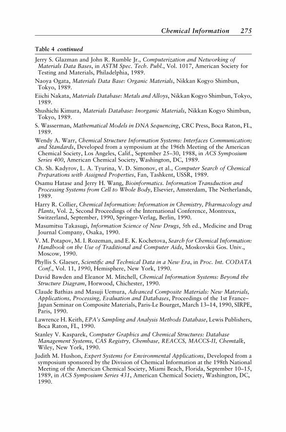
Table 4 continued

Jerry S. Glazman and John R. Rumble Jr., Computerization and Networking ofMaterials Data Bases, in ASTM Spec. Tech. Publ., Vol. 1017, American Society forTesting and Materials, Philadelphia, 1989.

Naoya Ogata, Materials Data Base: Organic Materials, Nikkan Kogyo Shimbun,Tokyo, 1989.

Eiichi Nakata, Materials Database: Metals and Alloys, Nikkan Kogyo Shimbun, Tokyo,1989.

Shushichi Kimura, Materials Database: Inorganic Materials, Nikkan Kogyo Shimbun,Tokyo, 1989.

S. Wasserman, Mathematical Models in DNA Sequencing, CRC Press, Boca Raton, FL,1989.

Wendy A. Warr, Chemical Structure Information Systems: Interfaces Communication;and Standards, Developed from a symposium at the 196th Meeting of the AmericanChemical Society, Los Angeles, Calif., September 25–30, 1988, in ACS SymposiumSeries 400, American Chemical Society, Washington, DC, 1989.

Ch. Sh. Kadyrov, L. A. Tyurina, V. D. Simonov, et al., Computer Search of ChemicalPreparations with Assigned Properties, Fan, Tashkent, USSR, 1989.

Osamu Hatase and Jerry H. Wang, Bioinformatics. Information Transduction andProcessing Systems from Cell to Whole Body, Elsevier, Amsterdam, The Netherlands,1989.

Harry R. Collier, Chemical Information: Information in Chemistry, Pharmacology andPlants, Vol. 2, Second Proceedings of the International Conference, Montreux,Switzerland, September, 1990, Springer-Verlag, Berlin, 1990.

Masumitsu Takasugi, Information Science of New Drugs, 5th ed., Medicine and DrugJournal Company, Osaka, 1990.

V. M. Potapov, M. I. Rozeman, and E. K. Kochetova, Search for Chemical Information:Handbook on the Use of Traditional and Computer Aids, Moskovskii Gos. Univ.,Moscow, 1990.

Phyllis S. Glaeser, Scientific and Technical Data in a New Era, in Proc. Int. CODATAConf., Vol. 11, 1990, Hemisphere, New York, 1990.

David Bawden and Eleanor M. Mitchell, Chemical Information Systems: Beyond theStructure Diagram, Horwood, Chichester, 1990.

Claude Bathias and Masuji Uemura, Advanced Composite Materials: New Materials,Applications, Processing, Evaluation and Databases, Proceedings of the 1st France–Japan Seminar on Composite Materials, Paris-Le Bourget, March 13–14, 1990, SIRPE,Paris, 1990.

Lawrence H. Keith, EPA’s Sampling and Analysis Methods Database, Lewis Publishers,Boca Raton, FL, 1990.

Stanley V. Kasparek, Computer Graphics and Chemical Structures: DatabaseManagement Systems, CAS Registry, Chembase, REACCS, MACCS-II, Chemtalk,Wiley, New York, 1990.

Judith M. Hushon, Expert Systems for Environmental Applications, Developed from asymposium sponsored by the Division of Chemical Information at the 198th NationalMeeting of the American Chemical Society, Miami Beach, Florida, September 10–15,1989, in ACS Symposium Series 431, American Chemical Society, Washington, DC,1990.

Chemical Information 275

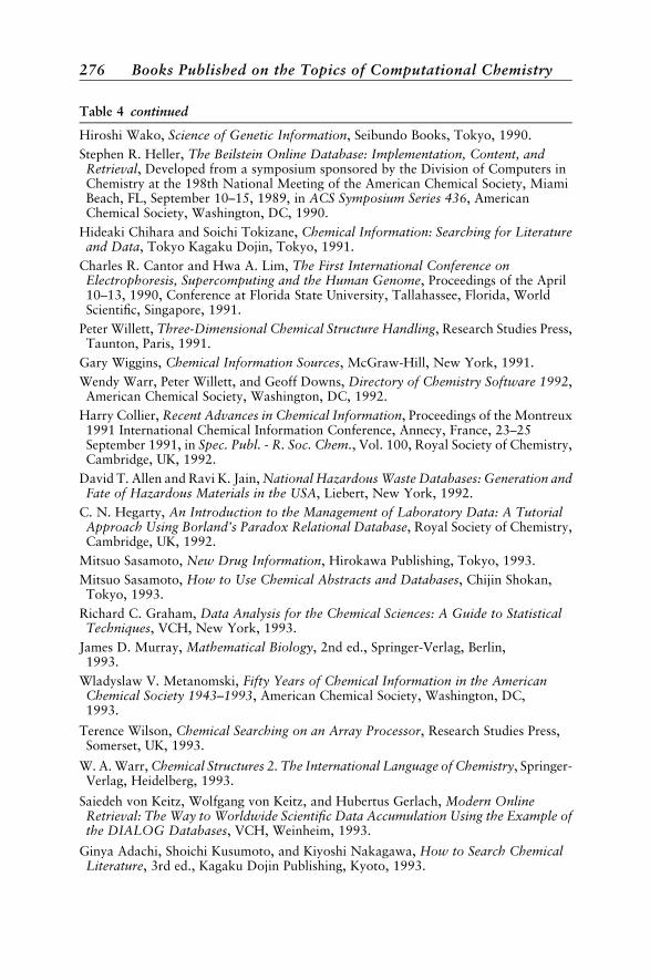
Table 4 continued

Hiroshi Wako, Science of Genetic Information, Seibundo Books, Tokyo, 1990.

Stephen R. Heller, The Beilstein Online Database: Implementation, Content, andRetrieval, Developed from a symposium sponsored by the Division of Computers inChemistry at the 198th National Meeting of the American Chemical Society, MiamiBeach, FL, September 10–15, 1989, in ACS Symposium Series 436, AmericanChemical Society, Washington, DC, 1990.

Hideaki Chihara and Soichi Tokizane, Chemical Information: Searching for Literatureand Data, Tokyo Kagaku Dojin, Tokyo, 1991.

Charles R. Cantor and Hwa A. Lim, The First International Conference onElectrophoresis, Supercomputing and the Human Genome, Proceedings of the April10–13, 1990, Conference at Florida State University, Tallahassee, Florida, WorldScientific, Singapore, 1991.

Peter Willett, Three-Dimensional Chemical Structure Handling, Research Studies Press,Taunton, Paris, 1991.

Gary Wiggins, Chemical Information Sources, McGraw-Hill, New York, 1991.

Wendy Warr, Peter Willett, and Geoff Downs, Directory of Chemistry Software 1992,American Chemical Society, Washington, DC, 1992.

Harry Collier, Recent Advances in Chemical Information, Proceedings of the Montreux1991 International Chemical Information Conference, Annecy, France, 23–25September 1991, in Spec. Publ. - R. Soc. Chem., Vol. 100, Royal Society of Chemistry,Cambridge, UK, 1992.

David T. Allen and Ravi K. Jain, National Hazardous Waste Databases: Generation andFate of Hazardous Materials in the USA, Liebert, New York, 1992.

C. N. Hegarty, An Introduction to the Management of Laboratory Data: A TutorialApproach Using Borland’s Paradox Relational Database, Royal Society of Chemistry,Cambridge, UK, 1992.

Mitsuo Sasamoto, New Drug Information, Hirokawa Publishing, Tokyo, 1993.

Mitsuo Sasamoto, How to Use Chemical Abstracts and Databases, Chijin Shokan,Tokyo, 1993.

Richard C. Graham, Data Analysis for the Chemical Sciences: A Guide to StatisticalTechniques, VCH, New York, 1993.

James D. Murray, Mathematical Biology, 2nd ed., Springer-Verlag, Berlin,1993.

Wladyslaw V. Metanomski, Fifty Years of Chemical Information in the AmericanChemical Society 1943–1993, American Chemical Society, Washington, DC,1993.

Terence Wilson, Chemical Searching on an Array Processor, Research Studies Press,Somerset, UK, 1993.

W. A. Warr, Chemical Structures 2. The International Language of Chemistry, Springer-Verlag, Heidelberg, 1993.

Saiedeh von Keitz, Wolfgang von Keitz, and Hubertus Gerlach, Modern OnlineRetrieval: The Way to Worldwide Scientific Data Accumulation Using the Example ofthe DIALOG Databases, VCH, Weinheim, 1993.

Ginya Adachi, Shoichi Kusumoto, and Kiyoshi Nakagawa, How to Search ChemicalLiterature, 3rd ed., Kagaku Dojin Publishing, Kyoto, 1993.

276 Books Published on the Topics of Computational Chemistry

Table 4 continued

Harry Collier, Recent Advances in Chemical Information II, The Proceedings of theMontreux 1992 International Chemical Information Conference, held at Annecy,France, 19–21 October 1992, in Spec. Publ. - R. Soc. Chem., Vol. 120, Royal Society ofChemistry, Cambridge, UK, 1993.

Harry Collier, Proceedings of the Montreux 1993 International Chemical InformationConference, Proceedings of a conference held in Annecy, France, 18–20 October 1993,Infonortics, Calne, UK, 1993.

Catherine Pepperrell, Three-Dimensional Similarity Searching, Research Studies Press,Taunton, UK, 1994.

H. M. Cartwright, Applications of Artificial Intelligence in Chemistry, Maruzen Co.Ltd., Tokyo, 1994.

Rich Lysakowski and Charles E. Gragg, Computerized Chemical Data Standards:Databases, Data Interchange, and Information Systems. Papers presented at asymposium held in Atlanta, GA, May 5–6, 1993, ASTM, Philadelphia, 1994.

Xiangchun Yu, Chemical Literature and Its Searching, 2nd ed., Science Publ. House,Beijing, 1994.

Tadayoshi Yoshimura and Hideo Sakagami, Intelligible Information Technology inChemistry, Ohmsha, Tokyo, 1994.

Barney K. Huang, Computer Simulation Analysis of Biological and AgriculturalSystems, CRC Press, Boca Raton, FL, 1994.

Masaki Hoshida, Challenge to Genome Informatics, Kyoritsu Shuppan, Tokyo, 1994.

Anonymous, InfoChem CD-ROM, InfoChem, Munich, 1994.

Harry Collier, Further Advances in Chemical Information, Proceedings of the MontreuxInternational Chemical Information Conference, held at Annecy, France, 18–20October 1993, in Spec. Publ. - R. Soc. Chem., Vol. 142, Royal Society of Chemistry,Cambridge, UK, 1994.

Sandor Suhai, Computational Methods in Genome Research, Proceedings of anInternational Symposium on Computational Methods in Genome Research, held July1–4, 1992, in Heidelberg, Germany, Plenum, New York, 1994.

Douglas Wemp Smith, Biocomputing: Informatics and Genome Projects, AcademicPress, San Diego, 1994.

Annette M. Griffin and Hugh G. Griffin, Computer Analysis of Sequence Data, Part I,Humana, Totowa, NJ, 1994.

Steffen Schulze-Kremer, Advances in Molecular Bioinformatics, IOS Press, Amsterdam,The Netherlands, 1994.

Hedda Schulz and Ursula Georgy, From CA to CAS Online, 2nd ed., NichigaiAssociates, Tokyo, 1995.

Dietmar Schomburg and Uta Lessel, Bioinformatics: From Nucleic Acids and Proteinsto Cell Metabolism, Contributions to the Conference on Bioinformatics, held October9–11, 1995, in Braunschweig, Germany, in GBF Monogr., Vol. 18, VCH, Weinheim,1995.

Clifford A. Pickover, Visualizing Biological Information, World Scientific, Singapore,1995.

Shigeki Mitaku and Minoru Kanehisa, The Human Genome Project and Knowledge-Information Processing, Baifukan, Tokyo, 1995.

Chemical Information 277

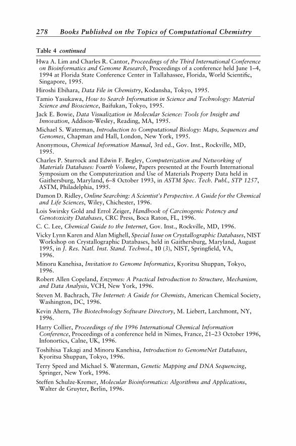
Table 4 continued

Hwa A. Lim and Charles R. Cantor, Proceedings of the Third International Conferenceon Bioinformatics and Genome Research, Proceedings of a conference held June 1–4,1994 at Florida State Conference Center in Tallahassee, Florida, World Scientific,Singapore, 1995.

Hiroshi Ebihara, Data File in Chemistry, Kodansha, Tokyo, 1995.

Tamio Yasukawa, How to Search Information in Science and Technology: MaterialScience and Bioscience, Baifukan, Tokyo, 1995.

Jack E. Bowie, Data Visualization in Molecular Science: Tools for Insight andInnovation, Addison-Wesley, Reading, MA, 1995.

Michael S. Waterman, Introduction to Computational Biology: Maps, Sequences andGenomes, Chapman and Hall, London, New York, 1995.

Anonymous, Chemical Information Manual, 3rd ed., Gov. Inst., Rockville, MD,1995.

Charles P. Sturrock and Edwin F. Begley, Computerization and Networking ofMaterials Databases: Fourth Volume, Papers presented at the Fourth InternationalSymposium on the Computerization and Use of Materials Property Data held inGaithersburg, Maryland, 6–8 October 1993, in ASTM Spec. Tech. Publ., STP 1257,ASTM, Philadelphia, 1995.

Damon D. Ridley, Online Searching: A Scientist’s Perspective. A Guide for the Chemicaland Life Sciences, Wiley, Chichester, 1996.

Lois Swirsky Gold and Errol Zeiger, Handbook of Carcinogenic Potency andGenotoxicity Databases, CRC Press, Boca Raton, FL, 1996.

C. C. Lee, Chemical Guide to the Internet, Gov. Inst., Rockville, MD, 1996.

Vicky Lynn Karen and Alan Mighell, Special Issue on Crystallographic Databases, NISTWorkshop on Crystallographic Databases, held in Gaithersburg, Maryland, August1995, in J. Res. Natl. Inst. Stand. Technol., 10 (3), NIST, Springfield, VA,1996.

Minoru Kanehisa, Invitation to Genome Informatics, Kyoritsu Shuppan, Tokyo,1996.

Robert Allen Copeland, Enzymes: A Practical Introduction to Structure, Mechanism,and Data Analysis, VCH, New York, 1996.

Steven M. Bachrach, The Internet: A Guide for Chemists, American Chemical Society,Washington, DC, 1996.

Kevin Ahern, The Biotechnology Software Directory, M. Liebert, Larchmont, NY,1996.

Harry Collier, Proceedings of the 1996 International Chemical InformationConference, Proceedings of a conference held in Nimes, France, 21–23 October 1996,Infonortics, Calne, UK, 1996.

Toshihisa Takagi and Minoru Kanehisa, Introduction to GenomeNet Databases,Kyoritsu Shuppan, Tokyo, 1996.

Terry Speed and Michael S. Waterman, Genetic Mapping and DNA Sequencing,Springer, New York, 1996.

Steffen Schulze-Kremer, Molecular Bioinformatics: Algorithms and Applications,Walter de Gruyter, Berlin, 1996.

278 Books Published on the Topics of Computational Chemistry

Table 4 continued

Leonard F. Peruski Jr. and Anne Harwood Peruski, The Internet and the New Biology:Tools for Genomic and Molecular Research, ASM Press, Herdon, VA, 1997.

Satoshi Nishijima and Shuichi Iwata, Computerization and Networking of MaterialsDatabases: Fifth Volume, Fifth International Symposium held in Tsukuba, Japan, 6–8November 1995, in ASTM Spec. Tech. Publ., STP 1311, ASTM, Philadelphia, 1997.

Satoru Miyano and Toshihisa Takagi, Proceedings of the Eighth Workshop on GenomeInformatics (GIW ’97), Proceedings of a conference held 12–13 December 1997, atYebisu Garden Place, Tokyo, in Genome Inf. Ser., Vol. 8, Universal Academy Press,Tokyo, 1997.

Brian Ellis and S. M. Jeffery, Polymers on CD-ROM: A Database of Commercial andScientific Information on Polymers and Polymeric Materials, Chapman & Hall,London, 1997.

William R. Crowley, Chemicals on the Internet, Vol. 1, Gulf, Houston, TX, 1997.

William Crowley, Chemicals on the Internet, Vol. 2: Inorganic Chemicals and Minerals,Gulf, Houston, TX, 1997.

Anonymous, Bioinformatics and the Effective Use of the Internet for Rapid DrugDiscovery, Proceedings of IBC’s International Conference held 3–4 March 1997, inSan Diego, California, IBC, Southborough, MA, 1997.

Anonymous, Functional Genomics: Drug Discovery from Gene to Screen, IBC,Southborough, MA, 1997.

Anonymous, AHFS Drug Information 97, Dtsch. Apoth. Verlag, Stuttgart, 1997.

R. Hofestadt and H. A. Lim, Molecular Bioinformatics: Sequence Analysis—TheHuman Genome Project, Proceedings of the ACM International Conference onSupercomputing (ICS ’97), held at the University of Vienna, 7–11 July 1997, ShakerVerlg, Aachen, Germany, 1997.

Sandor Suhai, Theoretical and Computational Methods in Genome Research,Proceedings of the International Symposium held 24–27 March 1996, in Heidelberg,Germany, Plenum, New York, 1997.

Andreas D. Baxevanis and B. F. Francis Ouellette, Bioinformatics: A Practical Guide tothe Analysis of Genes and Proteins, Wiley, New York, 1998.

Robert E. Maizell, How to Find Chemical Information: A Guide for PracticingChemists, Educators, and Students, 3rd ed., Wiley, New York, 1998.

Steven Brenner and Fran Lewitter, Trends Guide to Bioinformatics, Elsevier, Oxford,UK, 1998.

Stephen R. Heller, The Beilstein System: Strategies for Effective Searching, AmericanChemical Society, Washington, DC, 1998.

S. Ataka, M. Tasumi, and I. Suzuki, Infrared and Raman Spectroscopy Literature DataBase: A Bibliography Covering the Period, June 1997–May 1998, in J. Mol. Struct.,472–473, Elsevier, Amsterdam, The Netherlands, 1998.

Anonymous, NIOSH Pocket Guide to Chemical Hazards and Other Databases,NIOSH, Cincinnati, OH, 1999.

Alain Henaut, Informatics and the Genome, in Comput. Chem., 23 (3–4), Elsevier,Oxford, UK, 1999.

Steven Misener and Steven A. Krawetz, Bioinformatics: Methods and Protocols,Humana, Totowa, NJ, 2000.

Chemical Information 279

Table 4 continued

K. Arai, H. Okayama, T. Shimizu, Y. Takao, T. Noda, K. Mikoshiba, and Y. Yazaki,SPN: Application of Genomic Information to Medicine and Drug Discovery and itsRapid Trends in Japan and Overseas, Yodosha Co. Ltd., Tokyo, 2000.

Michael Lutz and Terry Kenakin, Quantitative Molecular Pharmacology andInformatics in Drug Discovery, Wiley, New York, 2000.

COMPUTATIONAL CHEMISTRY

Table 5 Books in the General Area of Computational Chemistry

A. J. Hopfinger, Conformational Properties of Macromolecules, Academic Press,New York, 1973.

Anonymous, A Study of a National Center For Computation in Chemistry, NationalAcademy of Sciences, Washington, DC, 1974.

M. B. Hooper, Computational Methods in Classical and Quantum Physics, HemispherePublishing, Washington, DC, 1976.

Anonymous, Needs and Opportunities For the National Resource For Computation inChemistry (NRCC), National Academy of Sciences, Washington, DC, 1976.

Aage Fredenslund, Jurgen Gmehling, and Peter Rasmussen, Vapor–Liquid Equilibriumsusing UNIFAC. A Group-Contribution Method, Elsevier, Amsterdam, The Nether-lands, 1977.

J. Nuttall, Atomic Scattering Theory: Mathematical and Computational Aspects,Proceedings of a conference held at the University of Western Ontario, June 7–9, 1978,University of Western Ontario, Department of Physics, London, Ontario, 1978.

Peter Lykos, Computer Modeling of Matter, in ACS Symposium Series 86, AmericanChemical Society, Washington, DC, 1978.

Enrico Clementi, Computational Aspects for Large Chemical Systems, Springer-Verlag,Berlin, 1980.

Peter Politzer and Donald G. Truhlar, Chemical Applications of Atomic and MolecularElectrostatic Potentials, Plenum, New York, 1981.

A. C. Norris, Computational Chemistry: An Introduction to Numerical Methods,Wiley, Chichester, 1981.

V. A. Polukhin, V. F. Ukhov, and M. M. Dzugutov, Computer Modeling of theDynamics and Structure of Liquid Metals, Nauka, Moscow, 1981.

I. G. Csizmadia and R. Daudel, Computational Theoretical Organic Chemistry,Proceedings of the NATO Advanced Study Institute Held at Menton, France, June29-July 13, 1980, in NATO Advanced Study Institute Series, Vol. C 67, Reidel,Dordrecht, 1981.

I. K. Karpov, Physicochemical Modeling by Computer in Geochemistry, Nauka, Sib.Otd., Novosibirsk, USSR, 1981.

G. M. Crippen, Distance Geometry and Conformational Calculations, Wiley,New York, 1981.

280 Books Published on the Topics of Computational Chemistry

Table 5 continued

P. G. Khalatur and Yu. G. Papulov, ‘‘Computer-Aided Experiment’’ in the Conforma-tional Analysis of Polymers, Kalinin. Gos. Univ., Kalinin, USSR, 1982.

G. H. F. Diercksen and S. Wilson, Methods in Computational Molecular Physics, inNATO Advanced Science Institutes Series, Series C: Mathematical and PhysicalSciences, Vol. 113, Reidel, Dordrecht, 1983.

Y. H. Ohtsuki, Recent Theoretical (Computational) Developments in Atomic Collisionsin Solids, Based on a symposium held in Strasbourg, France, 14–16 July 1981, WorldScientific, Singapore, 1983.

I. S. Duff and J. K. Reid, Proceedings of the 2nd International Conference on Vector andParallel Processors in Computational Science, in Comput. Phys. Commun, 37 (1–3),North-Holland, Amsterdam, The Netherlands, 1985.

Tim Clark, A Handbook of Computational Chemistry. A Practical Guide to ChemicalStructure and Energy Calculations, Wiley-Interscience, New York, 1985.

J. Broughton, W. Krakow, and S. T. Pantelides, Computer-Based Microscopic SymposiaProceedings, Vol. 63: Computer-Based Microscopic Description of the Structure andProperties of Materials, Based on a symposium held December 2–4, 1985, Boston,Mass., USA, in Materials Research Society Symposia Proceedings, Vol. 63, MaterialsResearch Society, Pittsburgh, PA, 1986.

W. J. Dunn, J. H. Block, and R. S. Pearlman, Partition Coefficient: Determination andEstimation, Pergamon, New York, 1986.

Hidehiko Nakano, Molecular Graphics, Science House, Tokyo, 1987.

P. G. Mezey, Potential Energy Hypersurfaces, Elsevier, Amsterdam, The Netherlands, 1987.

Klavs F. Jensen and Donald G. Truhlar, Supercomputer Research in Chemistry andChemical Engineering, Developed from a symposium held March 16–17, 1987, inMinneapolis, MN, in ACS Symposium Series 353, American Chemical Society,Washington, DC, 1987.

Tim Clark, A Handbook of Computational Chemistry, Maruzen, Tokyo, 1988.

J. Andrew McCammon and George L. Wilcox, Supercomputing in Biology: Proteins,Nucleic Acids, and Water, Selected papers from the Minnesota Conference, September13–16, 1987, Minneapolis, Minn., USA, in J. Comput.-Aided Mol. Design, 1 (4),ESCOM Science Publishers, Leiden, The Netherlands, 1988.

G. M. Crippen and T. F. Havel, Distance Geometry and Molecular Conformations,Wiley, New York, 1988.

Stephen Wilson, Concurrent Computation in Chemical Calculations, in Methods inComputational Chemistry, Vol. 3, Plenum, New York, 1989.

W. T. Thompson, F. Ajersch, and G. Eriksson, Proceedings of the InternationalSymposium on Computer Software in Chemical and Extractive Metallurgy, Basedupon a conference in Montreal, Canada, August 28–31, 1988, Pergamon, New York, 1989.

Enrico Clementi, MOTECC-89: Modern Techniques in Computer Chemistry, ESCOM,Leiden, 1989.

Enrico Clementi, Modern Techniques in Computational Chemistry: MOTECC-90,ESCOM, Leiden, 1990.

Kenny B. Lipkowitz and Donald B. Boyd, Reviews in Computational Chemistry, VCH,New York, 1990.

David M. Hirst, A Computational Approach to Chemistry, Blackwell Scientific, Oxford,UK, 1990.

Computational Chemistry 281

Table 5 continued

C. R. A. Catlow, S. C. Parker, and M. P. Allen, Computer Modeling of Fluids, Polymers,and Solids, in NATO ASI Series, Ser. C: Mathematical and Physical Sciences, Vol. 293,Kluwer, Dordrecht, 1990.

Tim Clark, Computer Chemistry: Practical Manual on Calculations of Structure andEnergy of Molecules, Mir, Moscow, 1990.

Arieh Warshel, Computer Modeling of Chemical Reactions in Enzymes and Solutions,Wiley, New York, 1991.

Kenny B. Lipkowitz and Donald B. Boyd, Reviews in Computational Chemistry, Vol. 2,VCH, New York, 1991.

Cemil Oegretir, Imre G. Csizmadia, and Emilia A. Lang, Computational Advances inOrganic Chemistry: Molecular Structure and Reactivity, Proceedings of the NATOAdvanced Study Institute on Computational Advances in Organic Chemistry:Molecular Structure and Reactivity, Altinoluk, Edremit, Turkey, July 31–August 12,1989, in NATO ASI Series C: Mathematical and Physical Sciences, Vol. 338, Kluwer,Dordrecht, 1991.

Enrico Clementi, Modern Techniques in Computational Chemistry: MOTECC-91,ESCOM, Leiden, 1991.

Sebastiao J. Formosinho, Imre G. Csizmadia, and Luis G. Arnaut, Theoretical andComputational Models for Organic Chemistry, Proceedings of the NATO AdvancedStudy Institute on Theoretical and Computational Models for Organic Chemistry,Praia de Porto Novo, Portugal, August 26–September 8, 1990, in NATO ASI Series.Series C: Mathematical and Physical Sciences, Vol. 339, Kluwer, Dordrecht, 1991.

Stephen Wilson and Geerd H. F. Diercksen, Methods in Computational MolecularPhysics, Proceedings of a NATO Advanced Study Institute on Methods inComputational Molecular Physics, held July 22–August 2, 1991, in Bad Windsheim,Germany, in NATO ASI Series, Ser. B., Vol. 293, Plenum, New York, 1992.

Stephen Wilson, Molecular Vibrations, in Methods in Computational Chemistry, Vol. 4,Plenum, New York, 1992.

Stephen Wilson, Atomic and Molecular Properties, in Methods in ComputationalChemistry, Vol. 5, Plenum, New York, 1992.

Jozef Bicerano, Computational Modeling of Polymers, in Plast. Eng. (N.Y.), Vol. 25,Dekker, New York, 1992.

L. A. Montero and Y. G. Smeyers, Trends in Applied Theoretical Chemistry, Kluwer,Dordrecht, 1992.

James E. Mark, Martin E. Glicksman, and Steven P. Marsh, Computational Methods inMaterials Science, Proceedings of a symposium, San Francisco, CA, 27 April–1 May1992, in Mater. Res. Soc. Symp. Proc., Vol. 278, Materials Research Society,Pittsburgh, PA, 1992.

J. Bertran, Molecular Aspects of Biotechnology: Computational Models andTheories, Proceedings of the NATO Advanced Research Workshop on The Role ofComputational Models and Theories in Biotechnology, Sant Feliu de Guixols, Spain,June 13–19, 1991, in NATO ASI Series, Ser. C., Vol. 368, Kluwer, Dordrecht, 1992.

Merry M. Ambos, Bruce R. Gelin, and Allen Richon, Computational Chemistry YellowPages, Molecular Solutions, Inc., St. Louis, MO, 1992.

S. Fraga, Computational Chemistry: Structure, Interactions and Reactivity, Part A, inStud. Phys. Theor. Chem., Vol. 77, Elsevier, Amsterdam, The Netherlands, 1992.

282 Books Published on the Topics of Computational Chemistry

Table 5 continued

Kenny B. Lipkowitz and Donald B. Boyd, Reviews in Computational Chemistry, Vol. 3,VCH, New York, 1992.

P. E. Bloechi, C. Joachim, and A. J. Fisher, Computations for the Nano-Scale,Proceedings of the Advanced Study Institute, Aspet, France, 12–16 October 1992, inNATO ASI Series, Ser. E, Vol. 240, Kluwer, Dordrecht, 1993.

W. J. Hehre, L. D. Burke, A. J. Shusterman, and W. J. Pietro, Experiments inComputational Organic Chemistry, Wavefunction, Inc., Irvine, CA, 1993.

Warren J. Hehre, Lonnie D. Burke, Alan J. Shusterman, A Spartan Tutorial,Wavefunction, Inc., Irvine, CA, 1993.

Kenny B. Lipkowitz and Donald B. Boyd, Reviews in Computational Chemistry, Vol. 4,VCH, New York, 1993.

Georges Wipff, Computational Approaches in Supramolecular Chemistry, Proceedingsof the NATO Advanced Research Workshop on Computational Approaches inSupramolecular Chemistry, ‘‘The Bischenberg’’ (near Strasbourg), France, September1–5, 1993, in NATO ASI Series, Ser. C, Vol. 426, Kluwer, Dordrecht, 1994.

Rudolf Janoschek and Imre G. Csizmadia, Recent Advances in Computational SiliconChemistry, in THEOCHEM, 119 (1), Elsevier, Amsterdam, The Netherlands, 1994.

Hugo O. Villar, Advances in Computational Biology, Vol. 1, JAI Press, Greenwich, CT,1994.

Anonymous, Annual Report of Chemical Software, 1994 ed., The Chemical SoftwareSociety of Japan, Sabae, Japan, 1994.

H. L. Sellers and J. T. Golab, Theoretical and Computational Approaches to InterfacePhenomena, Plenum, New York, 1994.

C. J. Cramer and D. G. Truhlar, Structure and Reactivity in Aqueous Solution.Characterization of Chemical and Biological Systems, in ACS Symposium Series 568,American Chemical Society, Washington, DC, 1994.

Eiji Osawa, Tsuneo Hirano, and Kazuhiko Honda, Computation Chemistry Series:Introduction to Computation Chemistry, Kodansha Ltd., Tokyo, Japan, 1994.

Douglas A. Smith, Modeling the Hydrogen Bond, Developed from a symposiumsponsored by the Division of Computers in Chemistry at the 206th National Meetingof the American Chemical Society, Chicago, Illinois, August 22–27, 1993, in ACSSymposium Series 569, American Chemical Society, Washington, DC, 1994.

Kenny B. Lipkowitz and Donald B. Boyd, Reviews in Computational Chemistry, Vol. 5,VCH, New York, 1994.

Fernando Bernardi and Jean-Louis Rivail, E.C.C.C. 1 Computational Chemistry,F.E.C.S. Conference in Nancy, France, May 1994, in AIP Conference Proceedings 330,AIP, Woodbury, NY, 1995.

Anonymous, Mathematical Challenges from Theoretical/Computational Chemistry,National Academy of Science Press, Washington, DC, 1995.

Anonymous, Annual Report of Chemical Software, 1995 ed., The Chemical SoftwareSociety of Japan, Sabae, Japan, 1995.

Steven M. Bachrach, William L. Hase, Donald B. Boyd, S. K. Gray, and Henry S. Rzepa,Eds., Proceedings of the First Electronic Computational Chemistry Conference, CDROM Version, Proceedings of a conference held exclusively on the Internet, November7–December 2, 1994, ARInternet Corporation, Landover, MD, 1995.

Computational Chemistry 283

Table 5 continued

D. W. Rogers, Computational Chemistry Using the PC, 2nd ed., VCH, Weinheim,1995.

Luciano Reatto and Franca Manghi, Progress in Computational Physics of Matter:Methods, Software and Applications, World Scientific, Singapore, 1995.

Winifred M. Huo and Franco A. Gianturco, Computational Methods for Electron-Molecule Collisions, Proceedings of the Workshop on Comparative Study of CurrentMethodologies in Electron-Molecule Scattering, held March 11–13, 1993, inCambridge, Massachusetts, Plenum, New York, 1995.

D. Neilson and M. P. Das, Computational Approaches to Novel Condensed MatterSystems: Applications to Classical and Quantum Systems, Proceedings of the ThirdGordon Godfrey International Workshop on Computational Approaches to NovelCondensed Matter Systems, held July 12–17, 1993, in Sydney, Australia, Plenum,New York, 1995.

W. J. Hehre and W. W. Huang, Chemistry with Computation, Wavefunction, Inc.,Irvine, CA, 1995.

W. J. Hehre, Practical Strategies for Electronic Structure Calculations, Wavefunction,Inc., Irvine, CA, 1995.

Timothy G. Mattson, Parallel Computing in Computational Chemistry, Developedfrom a symposium sponsored by the Division of Computers in Chemistry at the 207thNational Meeting of the American Chemical Society, San Diego, CA, March 13–17,1994, in ACS Symposium Series 592, American Chemical Society, Washington, DC,1995.

Guy H. Grant and W. Graham Richards, Computational Chemistry, Oxford UniversityPress, Oxford, UK, 1995.

Jerzy Leszczynski, Current Trends in Computational Chemistry, in Struct. Chem., 6(4–5), Plenum, New York, 1995.

Kenny B. Lipkowitz and Donald B. Boyd, Reviews in Computational Chemistry, Vol. 6,VCH, New York, 1995.

Lawrence Hunter and Teri E. Klein, Pacific Symposium on Biocomputing ‘96, Based ona Conference held in Hawaii, 3–6 January 1996, World Scientific, Singapore, 1996.

Jerzy Leszczynski, Computational Chemistry: Reviews of Current Trends, Vol. 1, WorldScientific, Singapore, 1996.

Michael Waterman, Introduction to Computational Biology; Maps, Sequences andGenomes, Chapman & Hall, London, UK, 1996.

Hugo O. Villar, Advances in Computational Biology, Vol. 2, JAI Press, Greenwich, CT,1996.

G. W. Robinson, S. Singh, and M. W. Evans, Water in Biology, Chemistry and Physics:Experimental Overviews and Computational Methodologies, World Scientific,Singapore, 1996.

Peter C. Jurs, Computer Software Applications in Chemistry, 2nd ed., Wiley, New York,1996.

W. J. Hehre, A. J. Shusterman, and W. W. Huang, A Laboratory Book ofComputational Organic Chemistry, Wavefunction, Inc., Irvine, CA, 1996.

Jane S. Murray and Kalidas Sen, Molecular Electrostatic Potentials: Concepts andApplications, in Theor. Comput. Chem., Vol. 3, Elsevier, Amsterdam, TheNetherlands, 1996.

284 Books Published on the Topics of Computational Chemistry

Table 5 continued

Kenneth M. Merz Jr. and Benoit Roux, Biological Membranes: A Molecular Perspectivefrom Computation and Experiment, Birkhauser, Cambridge, MA, 1996.

Kenny B. Lipkowitz and Donald B. Boyd, Reviews in Computational Chemistry, Vol. 7,VCH, New York, 1996.

Kenny B. Lipkowitz and Donald B. Boyd, Reviews in Computational Chemistry, Vol. 8,VCH, New York, 1996.

Kenny B. Lipkowitz and Donald B. Boyd, Reviews in Computational Chemistry, Vol. 9,VCH, New York, 1996.

S. M. Bachrach, Proceedings of the Second Electronic Computational Chemistry,Proceedings of a conference held 1–30 November 1995, in THEOCHEM, 368 (1–3),Elsevier, Amsterdam, The Netherlands, 1996.

Gerardo Cisneros, J. A. Cogordan, and Miguel Castro, Computational Chemistry andChemical Engineering, Proceedings of the Third UNAM–CRAY SupercomputingConference, held 13–16 August 1996, in Mexico, World Scientific, Singapore, 1997.

V. Fiorentini and F. Meloni, Proceedings of the VI Italian-Swiss Workshop on Advancesin Computational Materials Science, Proceedings of a conference held in S. Margheritadi Pula, (Cagliari), 28 September–2 October 1996, in Conf. Proc. - Ital. Phys. Soc., Vol.55, Ed Compos, Bologna, Italy, 1997.

Jerzy Leszczynski, Computational Chemistry: Reviews of Current Trends, Vol. 2, WorldScientific, Singapore, 1997.

Kazue Kurihara, The PRESTO Program: Structure and Functional Properties, Elsevier,Amsterdam, The Netherlands, 1997.

Andrzej K. Konopka, Open Problems of Computational Molecular Biology (5), inComput. Chem., 21 (4), Elsevier, Oxford, UK, 1997.

Stefan Balint, Analysis and Numerical Computation of Solutions of Nonlinear SystemsModeling Physical Phenomena, Especially: Nonlinear Optics, Inverse Problems,Mathematical Materials Science and Theoretical Fluid Mechanics, Proceedings of aconference held 19–21 May 1997, in Timisoara, Romania, University of the WestTimisoara, Timisoara, Romania, 1997.

S. M. Bachrach, Proceedings of the Third Electronic Computational ChemistryConference, Proceedings of a conference held 1–30 November 1996, in THEOCHEM,419, Elsevier, Amsterdam, The Netherlands, 1997.

Gabor Naray-Szabo and Arieh Warshel, Computational Approaches to BiochemicalReactivity, in Understanding Chem. React., Vol. 19, Kluwer, Dordrecht, 1997.

Saburo Nagakura and P. Rama Rao, India–Japan Joint Seminar on ComputationalMaterials Science, Based on a conference held 21–22 October 1996, in Hyderabad, inBull. Mater. Sci., 20 (6), Indian Academy of Sciences, Bangalore, 1997.

Ramesh Hariharan, Computational Biology, in J. Indian Inst. Sci., 77 (4), IndianInstitute of Science, Bangalore, 1997.

Pedro L. Garrido and Joacquin Marro, Fourth Granada Lectures in ComputationalPhysics, Proceedings of the 4th Granada Seminar held at Granada, Spain, 9–14September 1996, in Lect. Notes Phys., Vol. 493, Springer, Berlin, 1997.

Kenny B. Lipkowitz and Donald B. Boyd, Reviews in Computational Chemistry,Vol. 10, VCH, New York, 1997.

J.-M. Andre and D. H. Mosley, Exploring Aspects of Computational Chemistry:Concepts and Exercises, Presses Universitaires de Namur, Namur, Belgium, 1997.

Computational Chemistry 285

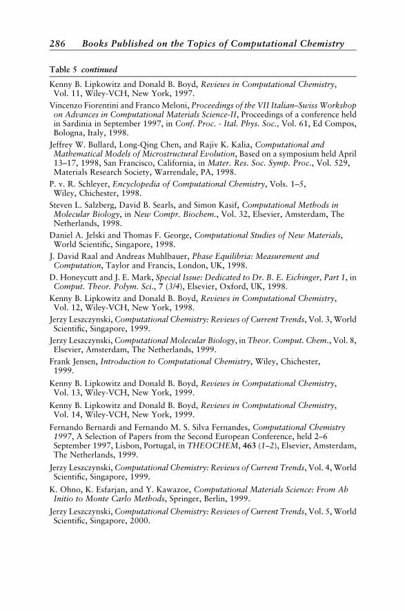
Table 5 continued

Kenny B. Lipkowitz and Donald B. Boyd, Reviews in Computational Chemistry,Vol. 11, Wiley-VCH, New York, 1997.

Vincenzo Fiorentini and Franco Meloni, Proceedings of the VII Italian–Swiss Workshopon Advances in Computational Materials Science-II, Proceedings of a conference heldin Sardinia in September 1997, in Conf. Proc. - Ital. Phys. Soc., Vol. 61, Ed Compos,Bologna, Italy, 1998.

Jeffrey W. Bullard, Long-Qing Chen, and Rajiv K. Kalia, Computational andMathematical Models of Microstructural Evolution, Based on a symposium held April13–17, 1998, San Francisco, California, in Mater. Res. Soc. Symp. Proc., Vol. 529,Materials Research Society, Warrendale, PA, 1998.

P. v. R. Schleyer, Encyclopedia of Computational Chemistry, Vols. 1–5,Wiley, Chichester, 1998.

Steven L. Salzberg, David B. Searls, and Simon Kasif, Computational Methods inMolecular Biology, in New Compr. Biochem., Vol. 32, Elsevier, Amsterdam, TheNetherlands, 1998.

Daniel A. Jelski and Thomas F. George, Computational Studies of New Materials,World Scientific, Singapore, 1998.

J. David Raal and Andreas Muhlbauer, Phase Equilibria: Measurement andComputation, Taylor and Francis, London, UK, 1998.

D. Honeycutt and J. E. Mark, Special Issue: Dedicated to Dr. B. E. Eichinger, Part 1, inComput. Theor. Polym. Sci., 7 (3/4), Elsevier, Oxford, UK, 1998.

Kenny B. Lipkowitz and Donald B. Boyd, Reviews in Computational Chemistry,Vol. 12, Wiley-VCH, New York, 1998.

Jerzy Leszczynski, Computational Chemistry: Reviews of Current Trends, Vol. 3, WorldScientific, Singapore, 1999.

Jerzy Leszczynski, Computational Molecular Biology, in Theor. Comput. Chem., Vol. 8,Elsevier, Amsterdam, The Netherlands, 1999.

Frank Jensen, Introduction to Computational Chemistry, Wiley, Chichester,1999.

Kenny B. Lipkowitz and Donald B. Boyd, Reviews in Computational Chemistry,Vol. 13, Wiley-VCH, New York, 1999.

Kenny B. Lipkowitz and Donald B. Boyd, Reviews in Computational Chemistry,Vol. 14, Wiley-VCH, New York, 1999.

Fernando Bernardi and Fernando M. S. Silva Fernandes, Computational Chemistry1997, A Selection of Papers from the Second European Conference, held 2–6September 1997, Lisbon, Portugal, in THEOCHEM, 463 (1–2), Elsevier, Amsterdam,The Netherlands, 1999.

Jerzy Leszczynski, Computational Chemistry: Reviews of Current Trends, Vol. 4, WorldScientific, Singapore, 1999.

K. Ohno, K. Esfarjan, and Y. Kawazoe, Computational Materials Science: From AbInitio to Monte Carlo Methods, Springer, Berlin, 1999.

Jerzy Leszczynski, Computational Chemistry: Reviews of Current Trends, Vol. 5, WorldScientific, Singapore, 2000.

286 Books Published on the Topics of Computational Chemistry

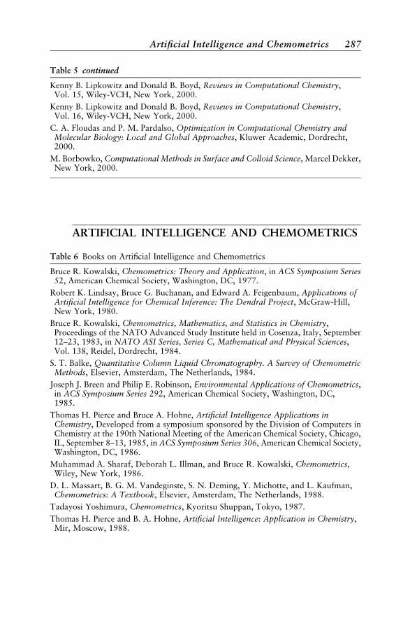
Table 5 continued

Kenny B. Lipkowitz and Donald B. Boyd, Reviews in Computational Chemistry,Vol. 15, Wiley-VCH, New York, 2000.

Kenny B. Lipkowitz and Donald B. Boyd, Reviews in Computational Chemistry,Vol. 16, Wiley-VCH, New York, 2000.

C. A. Floudas and P. M. Pardalso, Optimization in Computational Chemistry andMolecular Biology: Local and Global Approaches, Kluwer Academic, Dordrecht,2000.

M. Borbowko, Computational Methods in Surface and Colloid Science, Marcel Dekker,New York, 2000.

ARTIFICIAL INTELLIGENCE AND CHEMOMETRICS

Table 6 Books on Artificial Intelligence and Chemometrics

Bruce R. Kowalski, Chemometrics: Theory and Application, in ACS Symposium Series52, American Chemical Society, Washington, DC, 1977.

Robert K. Lindsay, Bruce G. Buchanan, and Edward A. Feigenbaum, Applications ofArtificial Intelligence for Chemical Inference: The Dendral Project, McGraw-Hill,New York, 1980.

Bruce R. Kowalski, Chemometrics, Mathematics, and Statistics in Chemistry,Proceedings of the NATO Advanced Study Institute held in Cosenza, Italy, September12–23, 1983, in NATO ASI Series, Series C, Mathematical and Physical Sciences,Vol. 138, Reidel, Dordrecht, 1984.

S. T. Balke, Quantitative Column Liquid Chromatography. A Survey of ChemometricMethods, Elsevier, Amsterdam, The Netherlands, 1984.

Joseph J. Breen and Philip E. Robinson, Environmental Applications of Chemometrics,in ACS Symposium Series 292, American Chemical Society, Washington, DC,1985.

Thomas H. Pierce and Bruce A. Hohne, Artificial Intelligence Applications inChemistry, Developed from a symposium sponsored by the Division of Computers inChemistry at the 190th National Meeting of the American Chemical Society, Chicago,IL, September 8–13, 1985, in ACS Symposium Series 306, American Chemical Society,Washington, DC, 1986.

Muhammad A. Sharaf, Deborah L. Illman, and Bruce R. Kowalski, Chemometrics,Wiley, New York, 1986.

D. L. Massart, B. G. M. Vandeginste, S. N. Deming, Y. Michotte, and L. Kaufman,Chemometrics: A Textbook, Elsevier, Amsterdam, The Netherlands, 1988.

Tadayosi Yoshimura, Chemometrics, Kyoritsu Shuppan, Tokyo, 1987.

Thomas H. Pierce and B. A. Hohne, Artificial Intelligence: Application in Chemistry,Mir, Moscow, 1988.

Artificial Intelligence and Chemometrics 287

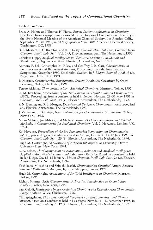
Table 6 continued

Bruce A. Hohne and Thomas H. Pierce, Expert System Applications in Chemistry,Developed from a symposium sponsored by the Division of Computers in Chemistry atthe 196th National Meeting of the American Chemical Society, Los Angeles, Calif.,September 25–30, 1988, in ACS Symposium Series 408, American Chemical Society,Washington, DC, 1989.

D. L. Massart, R. G. Brereton, and R. E. Dessy, Chemometrics Tutorials, Collected fromChemom. Intell. Lab. Syst., Vol. 1–5, Elsevier, Amsterdam, The Netherlands, 1990.

Zdzislaw Hippe, Artificial Intelligence in Chemistry: Structure Elucidation andSimulation of Organic Reactions, Elsevier, Amsterdam, Neth., 1991.

Anthony F. Fell, Christopher M. Riley, and Geoffrey P. R. Carr, Chemometrics inPharmaceutical and Biomedical Analysis, Proceedings from the InternationalSymposium, November 1990, Stockholm, Sweden, in J. Pharm. Biomed. Anal., 9 (8),Pergamon, Oxford, UK, 1991.

E. Morgan, Chemometrics: Experimental Design (Analytical Chemistry by OpenLearning), Wiley, Chichester, 1991.

Tetsuo Aishima, Chemometrics: New Analytical Chemistry, Maruzen, Tokyo, 1992.

O. M. Kvalheim, Proceedings of the 2nd Scandinavian Symposium on Chemometrics(SSC2), Proceedings from a conference held in Bergen, Norway, 28–31 May 1991 inChemom. Intell. Lab. Syst., 14 (1), Elsevier, Amsterdam, The Netherlands, 1992.

S. N. Deming and S. L. Morgan, Experimental Design: A Chemometric Approach, 2nded., Elsevier, Amsterdam, The Netherlands, 1993.

J. Zupan and J. Gasteiger, Neural Networks for Chemists—An Introduction, Wiley,New York, 1993.

Milan Meloun, Jiri Militky, and Michele Forina, PC-Aided Regression and RelatedMethods, in Chemometrics for Analytical Chemistry, Vol. 2, Horwood, London, UK,1994.

Kaj Heydorn, Proceedings of the 3rd Scandinavian Symposium on Chemometrics(SSC3), proceedings of a conference held in Aarhus, Denmark, 13–17 June 1993, inChemom. Intell. Lab. Syst., 23 (1), Elsevier, Amsterdam, The Netherlands, 1994.

Hugh M. Cartwright, Applications of Artificial Intelligence in Chemistry, OxfordUniversity Press, New York, 1994.

R. A. Felder, Third Symposium on Automation, Robotics and Artificial IntelligenceApplied to Analytical Chemistry and Laboratory Medicine, Based on a conference heldin San Diego, CA, 15–18 January 1994, in Chemom. Intell. Lab. Syst., 26 (2), Elsevier,Amsterdam, The Netherlands, 1994.

Yoshikatsu Miyashita and Shinichi Sasaki, Chemometrics: Chemical Pattern Recogni-tion and Multivariate Analysis, Kyoritsu Shuppan, Tokyo, 1995.

Hugh M. Cartwright, Applications of Artificial Intelligence in Chemistry, Maruzen,Tokyo, 1995.

Richard Kramer, Basic Chemometrics: A Practical Introduction to QuantitativeAnalysis, Wiley, New York, 1995.

Paul Geladi, Multivariate Image Analysis in Chemistry and Related Areas: ChemometricImage Analysis, Wiley, Chichester, 1996.

Cliff Spiegelman, Third International Conference on Environmetrics and Chemo-metrics, Based on a conference held in Las Vegas, Nevada, 11–13 September 1995, inChemom. Intell. Lab. Syst., 37 (1), Elsevier, Amsterdam, The Netherlands, 1997.

288 Books Published on the Topics of Computational Chemistry

Table 6 continued

Roman Kaliszan, Structure and Retention in Chromatography: A ChemometricApproach, Harwood, Amsterdam, The Netherlands, 1997.

Juergen W. Einax, Heinz W. Zwanziger, and Sabine Geiss, Chemometrics inEnvironmental Analysis, VCH, Weinheim, 1997.

D. L. Massart, B. G. M. Vandeginste, and L. M. C. Buydens, Handbook ofChemometrics and Qualimetrics, Part A, Elsevier, Oxford, UK, 1997.

D. L. Massart, B. G. M. Vandeginste, and L. M. C. Buydens, Handbook ofChemometrics and Qualimetrics, Part B, Elsevier, Oxford, UK, 1998.

Kenneth R. Beebe, Randy J. Pell, and Mary Beth Seasholtz, Chemometrics: A PracticalGuide, Wiley, New York, 1998.

J. Inczedy and D. L. Massart, CC ’97: Conferentia Chemometrica, Based on aconference held 21–23 August 1997, Budapest, Hungary, in Chemom. Intell. Lab.Syst., 47 (2), Elsevier, Amsterdam, The Netherlands, 1999.

Otto Matthias, Chemometrics: Statistics and Computer Application in AnalyticalChemistry, Wiley-VCH, Weinheim, 1998.

Khalid J. Siddiqui and DeLyle Eastwood, Pattern Recognition, Chemometrics, andImaging for Optical Environmental Monitoring. Proceedings of a symposium held20–21 September 1999 in Boston, Mass. Proc. SPIE-Int. Soc. Opt. Eng., Vol. 3854,1999.

Peter C. Meier and R. W. Johnson, Statistical Methods in Analytical Chemistry, 2nd ed.,Wiley, New York, 1999.

K. H. Esbensen, Special Issue: Proceedings of the 6th Scandinavian Symposium onChemometrics. Symposium held August 1999, Porsgrunn, Norway. J. Chemom., 14(5–6), 2000.

Jure Zupan and Johann Gasteiger, Neural Networks for Chemists, 2nd ed., Wiley, NewYork, 2000.

D. E. Clark, Evolutionary Algorithms in Molecular Design, Wiley-VCH, Weinheim,Germany, 2000.

CRYSTALLOGRAPHY, SPECTROSCOPY,AND THERMOCHEMISTRY

Table 7 Computational Chemistry Books in Crystallography, Spectroscopy, andThermochemistry

L. A. Gribov, Introduction to the Theory and Computation of Vibration Spectra ofPolyatomic Molecules, Leningradsk. Gos. Univ., Leningrad, 1965.

David P. Shoemaker, World List of Crystallographic Computer Programs, 2nd ed.,Polycrystal Book Service, Pittsburgh, PA, 1966.

Bonnie J. McBride and Sanford Gordon, FORTRAN IV Program for Calculation ofThermodynamic Data, CFSTI, Springfield, VA, 1967.

Richard Norman Jones, Computer Programs for Absorption Spectrophotometry,National Research Council of Canada, Ottawa, 1968.

Crystallography, Spectroscopy, and Thermochemistry 289

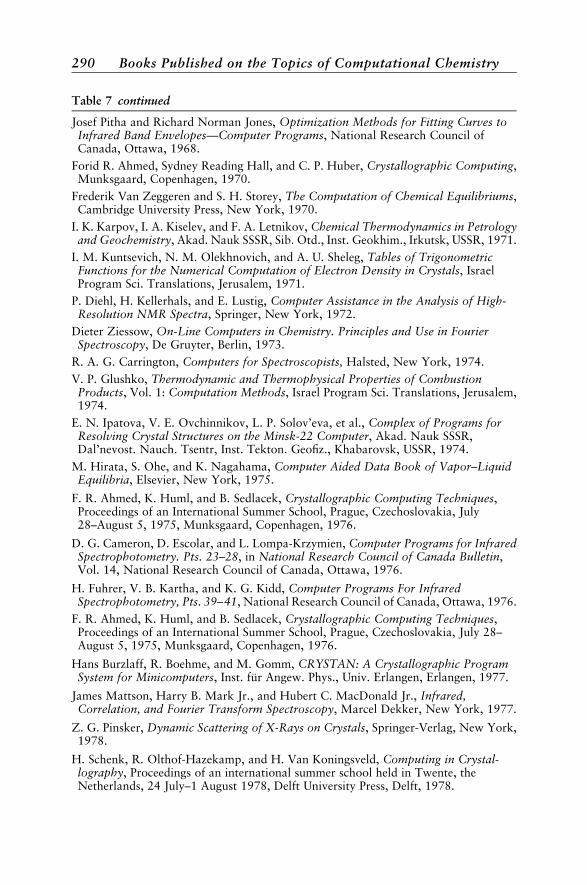
Table 7 continued

Josef Pitha and Richard Norman Jones, Optimization Methods for Fitting Curves toInfrared Band Envelopes—Computer Programs, National Research Council ofCanada, Ottawa, 1968.

Forid R. Ahmed, Sydney Reading Hall, and C. P. Huber, Crystallographic Computing,Munksgaard, Copenhagen, 1970.

Frederik Van Zeggeren and S. H. Storey, The Computation of Chemical Equilibriums,Cambridge University Press, New York, 1970.

I. K. Karpov, I. A. Kiselev, and F. A. Letnikov, Chemical Thermodynamics in Petrologyand Geochemistry, Akad. Nauk SSSR, Sib. Otd., Inst. Geokhim., Irkutsk, USSR, 1971.

I. M. Kuntsevich, N. M. Olekhnovich, and A. U. Sheleg, Tables of TrigonometricFunctions for the Numerical Computation of Electron Density in Crystals, IsraelProgram Sci. Translations, Jerusalem, 1971.

P. Diehl, H. Kellerhals, and E. Lustig, Computer Assistance in the Analysis of High-Resolution NMR Spectra, Springer, New York, 1972.

Dieter Ziessow, On-Line Computers in Chemistry. Principles and Use in FourierSpectroscopy, De Gruyter, Berlin, 1973.

R. A. G. Carrington, Computers for Spectroscopists, Halsted, New York, 1974.

V. P. Glushko, Thermodynamic and Thermophysical Properties of CombustionProducts, Vol. 1: Computation Methods, Israel Program Sci. Translations, Jerusalem,1974.

E. N. Ipatova, V. E. Ovchinnikov, L. P. Solov’eva, et al., Complex of Programs forResolving Crystal Structures on the Minsk-22 Computer, Akad. Nauk SSSR,Dal’nevost. Nauch. Tsentr, Inst. Tekton. Geofiz., Khabarovsk, USSR, 1974.

M. Hirata, S. Ohe, and K. Nagahama, Computer Aided Data Book of Vapor–LiquidEquilibria, Elsevier, New York, 1975.

F. R. Ahmed, K. Huml, and B. Sedlacek, Crystallographic Computing Techniques,Proceedings of an International Summer School, Prague, Czechoslovakia, July28–August 5, 1975, Munksgaard, Copenhagen, 1976.

D. G. Cameron, D. Escolar, and L. Lompa-Krzymien, Computer Programs for InfraredSpectrophotometry. Pts. 23–28, in National Research Council of Canada Bulletin,Vol. 14, National Research Council of Canada, Ottawa, 1976.

H. Fuhrer, V. B. Kartha, and K. G. Kidd, Computer Programs For InfraredSpectrophotometry, Pts. 39–41, National Research Council of Canada, Ottawa, 1976.

F. R. Ahmed, K. Huml, and B. Sedlacek, Crystallographic Computing Techniques,Proceedings of an International Summer School, Prague, Czechoslovakia, July 28–August 5, 1975, Munksgaard, Copenhagen, 1976.

Hans Burzlaff, R. Boehme, and M. Gomm, CRYSTAN: A Crystallographic ProgramSystem for Minicomputers, Inst. fur Angew. Phys., Univ. Erlangen, Erlangen, 1977.

James Mattson, Harry B. Mark Jr., and Hubert C. MacDonald Jr., Infrared,Correlation, and Fourier Transform Spectroscopy, Marcel Dekker, New York, 1977.

Z. G. Pinsker, Dynamic Scattering of X-Rays on Crystals, Springer-Verlag, New York,1978.

H. Schenk, R. Olthof-Hazekamp, and H. Van Koningsveld, Computing in Crystal-lography, Proceedings of an international summer school held in Twente, theNetherlands, 24 July–1 August 1978, Delft University Press, Delft, 1978.

290 Books Published on the Topics of Computational Chemistry

Table 7 continued

V. V. Serov, M. E. Elyashberg, and L. A. Gribov, System of Programs for IdentifyingChemical Compounds on the Basis of Molecular Spectra, VINITI, Moscow, 1978.

J. B. Pedley and J. Rylance, Sussex–N.P.L. Computer Analyzed Thermochemical Data:Organic and Organometallic Compounds, University of Sussex, Brighton, UK, 1979.

R. Diamond, S. Ramaseshan, and K. Venkatesan, Computing in Crystallography,Lectures delivered at the International Winter School on Crystallographic Computingheld in Bangalore, India, 4–14 January 1980, Indian Academy of Sciences, Bangalore,1980.

Yu. A. Osip’yan, Defects in Crystals and Their Computer-Aided Modeling, Nauka,Leningr. Otd., Leningrad, 1980.

M. E. Elyashberg, L. A. Gribov, and V. V. Serov, Molecular Spectrochemical Analysisand Computers, Nauka, Moscow, 1980.

Jong K. Lee, Interatomic Potentials and Crystalline Defects, Proceedings of asymposium sponsored by the TMS–AIME Chemistry and Physics of Metals Committeeand the MSD–ASM Computer Simulation Activity at the fall meeting of theMetallurgical Society of AIME, Pittsburgh, PA, October 6–7, 1980, MetallurgicalSociety AIME, Warrendale, PA, 1981.

David Sayre, Computational Crystallography, Clarendon Press, Oxford, UK, 1982.

Yu. V. Trushin, Computer and Modeling of Defects in Crystals, Akad. Nauk SSSR, Fiz.-Tekh. Inst., Leningrad, 1982.

V. I. Baranov, F. A. Savin, and L. A. Gribov, Programs for Calculation of Electron-Vibration Spectra of Polyatomic Molecules, Nauka, Moscow, 1983.

Yu. V. Trushin, Computer-Aided Modeling of Radiation Defects in Crystals, Akad.Nauk SSSR, Fiz.-Tekh. Inst., Leningrad, 1983.

Lester Haar, John S. Gallagher, and George S. Kell, NBS/NRC Steam Tables:Thermodynamic and Transport Properties and Computer Programs for Vapor andLiquid States of Water in SI Units, Hemisphere Publishing, Washington, DC, 1984.

S. R. Hall and T. Ashida, Methods and Applications in Crystallographic Computing,Papers presented at the International Summer School on Crystallographic Computingheld at Kyoto, Japan, 18–27 August 1983, Oxford University Press, Oxford, UK, 1984.

Yu. V. Trushin and U. G. Samsanidze, Evolution of the Defective Structure of Crystals(Computer-Aided Modeling), Akad. Nauk SSSR, Fiz.-Tekh. Inst., Leningrad, 1984.

G. M. Sheldrick, C. Krueger, and R. Goddard, Crystallographic Computing 3: DataCollection, Structure Determination, Proteins, and Databases, Papers presented at theInternational Summer School on Crystallographic Computing held in Muelheim an derRuhr, Federal Republic of Germany, 30 July–8 August, 1984, Clarendon Press,Oxford, UK, 1985.

Ole G. Mouritsen, Computer Studies of Phase Transitions and Critical Phenomena,Springer-Verlag, Berlin, 1984.

T. I. Barry, Chemical Thermodynamics in Industry: Models and Computation, inCritical Reports on Applied Chemistry, Vol. 8, Blackwell Scientific, Oxford, UK, 1985.

Paul Benedek and Francis Olti, Computer Aided Chemical Thermodynamics of Gasesand Liquids: Theory, Models, and Programs, Wiley, New York, 1985.

Jure Zupan, Computer-Supported Spectroscopic Databases, Ellis Horwood, Chichester,1986.

Crystallography, Spectroscopy, and Thermochemistry 291

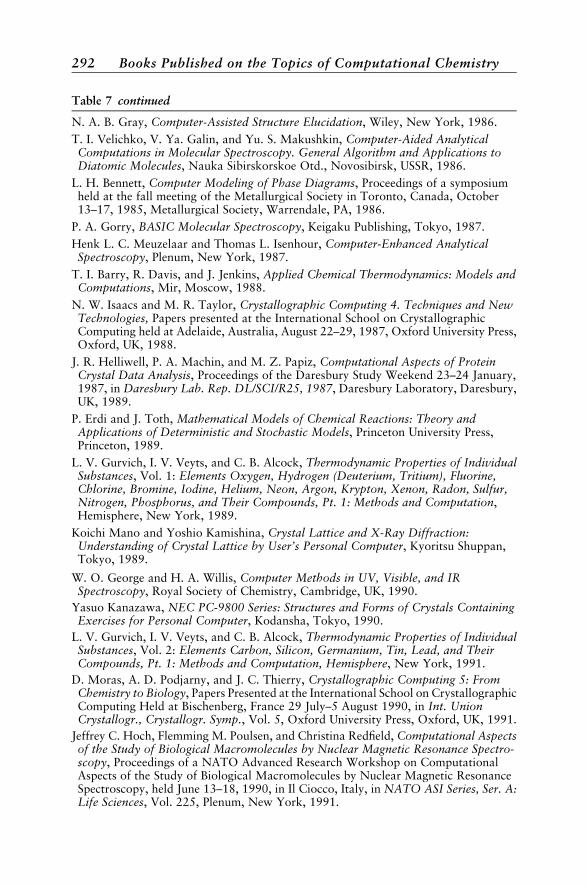
Table 7 continued

N. A. B. Gray, Computer-Assisted Structure Elucidation, Wiley, New York, 1986.

T. I. Velichko, V. Ya. Galin, and Yu. S. Makushkin, Computer-Aided AnalyticalComputations in Molecular Spectroscopy. General Algorithm and Applications toDiatomic Molecules, Nauka Sibirskorskoe Otd., Novosibirsk, USSR, 1986.

L. H. Bennett, Computer Modeling of Phase Diagrams, Proceedings of a symposiumheld at the fall meeting of the Metallurgical Society in Toronto, Canada, October13–17, 1985, Metallurgical Society, Warrendale, PA, 1986.

P. A. Gorry, BASIC Molecular Spectroscopy, Keigaku Publishing, Tokyo, 1987.

Henk L. C. Meuzelaar and Thomas L. Isenhour, Computer-Enhanced AnalyticalSpectroscopy, Plenum, New York, 1987.

T. I. Barry, R. Davis, and J. Jenkins, Applied Chemical Thermodynamics: Models andComputations, Mir, Moscow, 1988.

N. W. Isaacs and M. R. Taylor, Crystallographic Computing 4. Techniques and NewTechnologies, Papers presented at the International School on CrystallographicComputing held at Adelaide, Australia, August 22–29, 1987, Oxford University Press,Oxford, UK, 1988.

J. R. Helliwell, P. A. Machin, and M. Z. Papiz, Computational Aspects of ProteinCrystal Data Analysis, Proceedings of the Daresbury Study Weekend 23–24 January,1987, in Daresbury Lab. Rep. DL/SCI/R25, 1987, Daresbury Laboratory, Daresbury,UK, 1989.

P. Erdi and J. Toth, Mathematical Models of Chemical Reactions: Theory andApplications of Deterministic and Stochastic Models, Princeton University Press,Princeton, 1989.

L. V. Gurvich, I. V. Veyts, and C. B. Alcock, Thermodynamic Properties of IndividualSubstances, Vol. 1: Elements Oxygen, Hydrogen (Deuterium, Tritium), Fluorine,Chlorine, Bromine, Iodine, Helium, Neon, Argon, Krypton, Xenon, Radon, Sulfur,Nitrogen, Phosphorus, and Their Compounds, Pt. 1: Methods and Computation,Hemisphere, New York, 1989.

Koichi Mano and Yoshio Kamishina, Crystal Lattice and X-Ray Diffraction:Understanding of Crystal Lattice by User’s Personal Computer, Kyoritsu Shuppan,Tokyo, 1989.

W. O. George and H. A. Willis, Computer Methods in UV, Visible, and IRSpectroscopy, Royal Society of Chemistry, Cambridge, UK, 1990.

Yasuo Kanazawa, NEC PC-9800 Series: Structures and Forms of Crystals ContainingExercises for Personal Computer, Kodansha, Tokyo, 1990.

L. V. Gurvich, I. V. Veyts, and C. B. Alcock, Thermodynamic Properties of IndividualSubstances, Vol. 2: Elements Carbon, Silicon, Germanium, Tin, Lead, and TheirCompounds, Pt. 1: Methods and Computation, Hemisphere, New York, 1991.

D. Moras, A. D. Podjarny, and J. C. Thierry, Crystallographic Computing 5: FromChemistry to Biology, Papers Presented at the International School on CrystallographicComputing Held at Bischenberg, France 29 July–5 August 1990, in Int. UnionCrystallogr., Crystallogr. Symp., Vol. 5, Oxford University Press, Oxford, UK, 1991.

Jeffrey C. Hoch, Flemming M. Poulsen, and Christina Redfield, Computational Aspectsof the Study of Biological Macromolecules by Nuclear Magnetic Resonance Spectro-scopy, Proceedings of a NATO Advanced Research Workshop on ComputationalAspects of the Study of Biological Macromolecules by Nuclear Magnetic ResonanceSpectroscopy, held June 13–18, 1990, in Il Ciocco, Italy, in NATO ASI Series, Ser. A:Life Sciences, Vol. 225, Plenum, New York, 1991.

292 Books Published on the Topics of Computational Chemistry

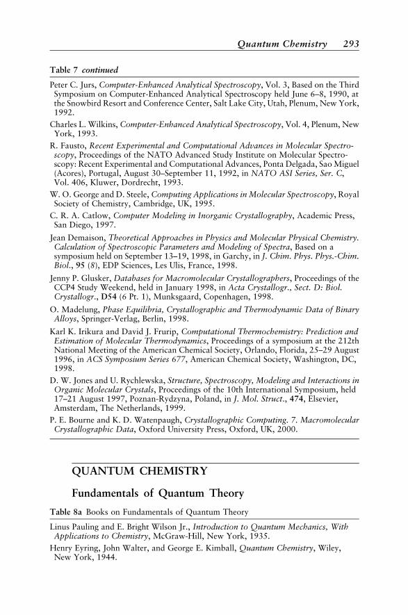
Table 7 continued

Peter C. Jurs, Computer-Enhanced Analytical Spectroscopy, Vol. 3, Based on the ThirdSymposium on Computer-Enhanced Analytical Spectroscopy held June 6–8, 1990, atthe Snowbird Resort and Conference Center, Salt Lake City, Utah, Plenum, New York,1992.

Charles L. Wilkins, Computer-Enhanced Analytical Spectroscopy, Vol. 4, Plenum, NewYork, 1993.

R. Fausto, Recent Experimental and Computational Advances in Molecular Spectro-scopy, Proceedings of the NATO Advanced Study Institute on Molecular Spectro-scopy: Recent Experimental and Computational Advances, Ponta Delgada, Sao Miguel(Acores), Portugal, August 30–September 11, 1992, in NATO ASI Series, Ser. C,Vol. 406, Kluwer, Dordrecht, 1993.

W. O. George and D. Steele, Computing Applications in Molecular Spectroscopy, RoyalSociety of Chemistry, Cambridge, UK, 1995.

C. R. A. Catlow, Computer Modeling in Inorganic Crystallography, Academic Press,San Diego, 1997.

Jean Demaison, Theoretical Approaches in Physics and Molecular Physical Chemistry.Calculation of Spectroscopic Parameters and Modeling of Spectra, Based on asymposium held on September 13–19, 1998, in Garchy, in J. Chim. Phys. Phys.-Chim.Biol., 95 (8), EDP Sciences, Les Ulis, France, 1998.

Jenny P. Glusker, Databases for Macromolecular Crystallographers, Proceedings of theCCP4 Study Weekend, held in January 1998, in Acta Crystallogr., Sect. D: Biol.Crystallogr., D54 (6 Pt. 1), Munksgaard, Copenhagen, 1998.

O. Madelung, Phase Equilibria, Crystallographic and Thermodynamic Data of BinaryAlloys, Springer-Verlag, Berlin, 1998.

Karl K. Irikura and David J. Frurip, Computational Thermochemistry: Prediction andEstimation of Molecular Thermodynamics, Proceedings of a symposium at the 212thNational Meeting of the American Chemical Society, Orlando, Florida, 25–29 August1996, in ACS Symposium Series 677, American Chemical Society, Washington, DC,1998.

D. W. Jones and U. Rychlewska, Structure, Spectroscopy, Modeling and Interactions inOrganic Molecular Crystals, Proceedings of the 10th International Symposium, held17–21 August 1997, Poznan-Rydzyna, Poland, in J. Mol. Struct., 474, Elsevier,Amsterdam, The Netherlands, 1999.

P. E. Bourne and K. D. Watenpaugh, Crystallographic Computing. 7. MacromolecularCrystallographic Data, Oxford University Press, Oxford, UK, 2000.

QUANTUM CHEMISTRY

Fundamentals of Quantum Theory

Table 8a Books on Fundamentals of Quantum Theory

Linus Pauling and E. Bright Wilson Jr., Introduction to Quantum Mechanics, WithApplications to Chemistry, McGraw-Hill, New York, 1935.

Henry Eyring, John Walter, and George E. Kimball, Quantum Chemistry, Wiley,New York, 1944.

Quantum Chemistry 293

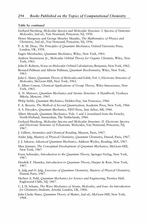
Table 8a continued

Gerhard Herzberg, Molecular Spectra and Molecular Structure. I. Spectra of DiatomicMolecules, 2nd ed., Van Nostrand, Princeton, NJ, 1950.

Henry Margenau and George Moseley Murphy, The Mathematics of Physics andChemistry, 2nd ed., Van Nostrand, Princeton, NJ, 1956.

P. A. M. Dirac, The Principles of Quantum Mechanics, Oxford University Press,London, UK, 1958.

Eugen Merzbacher, Quantum Mechanics, Wiley, New York, 1961.

Andrew Streitwieser Jr., Molecular Orbital Theory for Organic Chemists, Wiley, NewYork, 1961.

John D. Roberts, Notes on Molecular Orbital Calculations, Benjamin, New York, 1962.

Bernard Pullman and Alberte Pullman, Quantum Biochemistry, Wiley, New York,1963.

John C. Slater, Quantum Theory of Molecules and Solids, Vol. 1, Electronic Structure ofMolecules, McGraw-Hill, New York, 1963.

F. Albert Cotton, Chemical Applications of Group Theory, Wiley-Interscience, NewYork, 1963.

A. N. Matveev, Quantum Mechanics and Atomic Structure. A Handbook, VysshayaShkola, Moscow, 1965.

Philip Stehle, Quantum Mechanics, Holden-Day, San Francisco, 1966.

F. A. Berezin, The Method of Second Quantization, Academic Press, New York, 1966.

A. S. Davydov, Quantum Mechanics, NEO Press, Ann Arbor, MI, 1966.

Albert Messiah, Quantum Mechanics, Vols. 1 and 2 (translated from the French),North-Holland, Amsterdam, The Netherlands, 1966.

Gerhard Herzberg, Molecular Spectra and Molecular Structure. II. Electronic Spectraand Electronic Structure of Polyatomic Molecules, Van Nostrand, Princeton, NJ,1967.

J. Gilbert, Atomistics and Chemical Bonding, Masson, Paris, 1967.

Andre Julg, Mastery of Physical Chemistry, Quantum Chemistry, Dunod, Paris, 1967.

J. J. Sakurai, Advanced Quantum Mechanics, Addison-Wesley, Reading, MA, 1967.

Max Jammer, The Conceptual Development of Quantum Mechanics, McGraw-Hill,New York, 1967.

Franz Schneider, Introduction to the Quantum Theory, Springer-Verlag, New York,1967.

Hendrik F. Hameka, Introduction to Quantum Theory, Harper & Row, New York,1967.

A. Julg and O. Julg, Exercises of Quantum Chemistry, Mastery of Physical Chemistry,Dunod, Paris, 1967.

Herbert A. Pohl, Quantum Mechanics for Science and Engineering, Prentice Hall,Englewood Cliffs, NJ, 1967.

C. J. H. Schutte, The Wave Mechanics of Atoms, Molecules, and Ions: An Introductionfor Chemistry Students, Arnold, London, UK, 1968.

John Clarke Slater, Quantum Theory of Matter, 2nd ed., McGraw-Hill, New York,1968.

294 Books Published on the Topics of Computational Chemistry

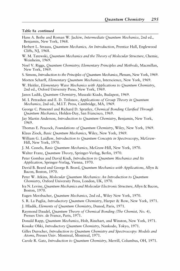
Table 8a continued

Hans A. Bethe and Roman W. Jackiw, Intermediate Quantum Mechanics, 2nd ed.,Benjamin, New York, 1968.

Herbert L. Strauss, Quantum Mechanics, An Introduction, Prentice Hall, EnglewoodCliffs, NJ, 1968.

W. M. Tatewski, Quantum Mechanics and the Theory of Molecular Structure, Chemie,Weinheim, 1969.

Noel V. Riggs, Quantum Chemistry; Elementary Principles and Methods, Macmillan,New York, 1969.

S. Simons, Introduction to the Principles of Quantum Mechanics, Plenum, New York, 1969.

Morten Scharff, Elementary Quantum Mechanics, Interscience, New York, 1969.

W. Heitler, Elementary Wave Mechanics with Applications to Quantum Chemistry,2nd ed., Oxford University Press, New York, 1969.

Janos Ladik, Quantum Chemistry, Muszaki Kiado, Budapest, 1969.

M. I. Petrashen and E. D. Trifonov, Applications of Group Theory in QuantumMechanics, 2nd ed., M.I.T. Press, Cambridge, MA, 1969.

George C. Pimentel and Richard D. Spratley, Chemical Bonding Clarified ThroughQuantum Mechanics, Holden-Day, San Francisco, 1969.

Jay Martin Anderson, Introduction to Quantum Chemistry, Benjamin, New York,1969.

Thomas E. Peacock, Foundations of Quantum Chemistry, Wiley, New York, 1969.

Klaus Ziock, Basic Quantum Mechanics, Wiley, New York, 1969.

William G. Laidlaw, Introduction to Quantum Concepts in Spectroscopy, McGraw-Hill, New York, 1970.

J. M. Cassels, Basic Quantum Mechanics, McGraw-Hill, New York, 1970.

Walter Franz, Quantum Theory, Springer-Verlag, Berlin, 1970.

Peter Gombas and David Kisdi, Introduction to Quantum Mechanics and ItsApplication, Springer-Verlag, Vienna, 1970.

David B. Beard and George B. Beard, Quantum Mechanics with Applications, Allyn &Bacon, Boston, 1970.

Peter W. Atkins, Molecular Quantum Mechanics: An Introduction to QuantumChemistry, Oxford University Press, London, UK, 1970.

Ira N. Levine, Quantum Mechanics and Molecular Electronic Structure, Allyn & Bacon,Boston, 1970.

Eugen Merzbacher, Quantum Mechanics, 2nd ed., Wiley New York, 1970.

S. R. La Paglia, Introductory Quantum Chemistry, Harper & Row, New York, 1971.

J. Hladik, Elements of Quantum Chemistry, Dunod, Paris, 1971.

Raymond Daudel, Quantum Theory of Chemical Bonding (The Chemist, No. 4),Presses Univ. de France, Paris, 1971.

Donald Rapp, Quantum Mechanics, Holt, Rinehart, and Winston, New York, 1971.

Kosuke Ohki, Introductory Quantum Chemistry, Nankodo, Tokyo, 1971.

Gilles Durocher, Introduction to Quantum Chemistry and Spectroscopy: Models andAtoms, Presses Univ. Montreal, Montreal, 1971.

Carole R. Gatz, Introduction to Quantum Chemistry, Merrill, Columbus, OH, 1971.

Quantum Chemistry 295

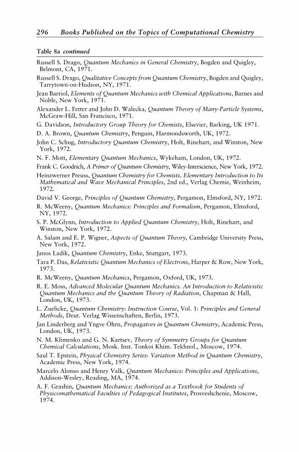
Table 8a continued

Russell S. Drago, Quantum Mechanics in General Chemistry, Bogden and Quigley,Belmont, CA, 1971.

Russell S. Drago, Qualitative Concepts from Quantum Chemistry, Bogden and Quigley,Tarrytown-on-Hudson, NY, 1971.

Jean Barriol, Elements of Quantum Mechanics with Chemical Applications, Barnes andNoble, New York, 1971.

Alexander L. Fetter and John D. Walecka, Quantum Theory of Many-Particle Systems,McGraw-Hill, San Francisco, 1971.

G. Davidson, Introductory Group Theory for Chemists, Elsevier, Barking, UK 1971.

D. A. Brown, Quantum Chemistry, Penguin, Harmondsworth, UK, 1972.

John C. Schug, Introductory Quantum Chemistry, Holt, Rinehart, and Winston, NewYork, 1972.

N. F. Mott, Elementary Quantum Mechanics, Wykeham, London, UK, 1972.

Frank C. Goodrich, A Primer of Quantum Chemistry, Wiley-Interscience, New York, 1972.

Heinzwerner Preuss, Quantum Chemistry for Chemists. Elementary Introduction to ItsMathematical and Wave Mechanical Principles, 2nd ed., Verlag Chemie, Weinheim,1972.

David V. George, Principles of Quantum Chemistry, Pergamon, Elmsford, NY, 1972.

R. McWeeny, Quantum Mechanics: Principles and Formalism, Pergamon, Elmsford,NY, 1972.

S. P. McGlynn, Introduction to Applied Quantum Chemistry, Holt, Rinehart, andWinston, New York, 1972.

A. Salam and E. P. Wigner, Aspects of Quantum Theory, Cambridge University Press,New York, 1972.

Janos Ladik, Quantum Chemistry, Enke, Stuttgart, 1973.

Tara P. Das, Relativistic Quantum Mechanics of Electrons, Harper & Row, New York,1973.

R. McWeeny, Quantum Mechanics, Pergamon, Oxford, UK, 1973.

R. E. Moss, Advanced Molecular Quantum Mechanics. An Introduction to RelativisticQuantum Mechanics and the Quantum Theory of Radiation, Chapman & Hall,London, UK, 1973.

L. Zuelicke, Quantum Chemistry: Instruction Course, Vol. 1: Principles and GeneralMethods, Deut. Verlag Wissenschaften, Berlin, 1973.

Jan Linderberg and Yngve Ohrn, Propagators in Quantum Chemistry, Academic Press,London, UK, 1973.

N. M. Klimenko and G. N. Kartsev, Theory of Symmetry Groups for QuantumChemical Calculations, Mosk. Inst. Tonkoi Khim. Tekhnol., Moscow, 1974.

Saul T. Epstein, Physical Chemistry Series: Variation Method in Quantum Chemistry,Academic Press, New York, 1974.

Marcelo Alonso and Henry Valk, Quantum Mechanics: Principles and Applications,Addison-Wesley, Reading, MA, 1974.

A. F. Grashin, Quantum Mechanics: Authorized as a Textbook for Students ofPhysicomathematical Faculties of Pedagogical Institutes, Prosveshchenie, Moscow,1974.

296 Books Published on the Topics of Computational Chemistry

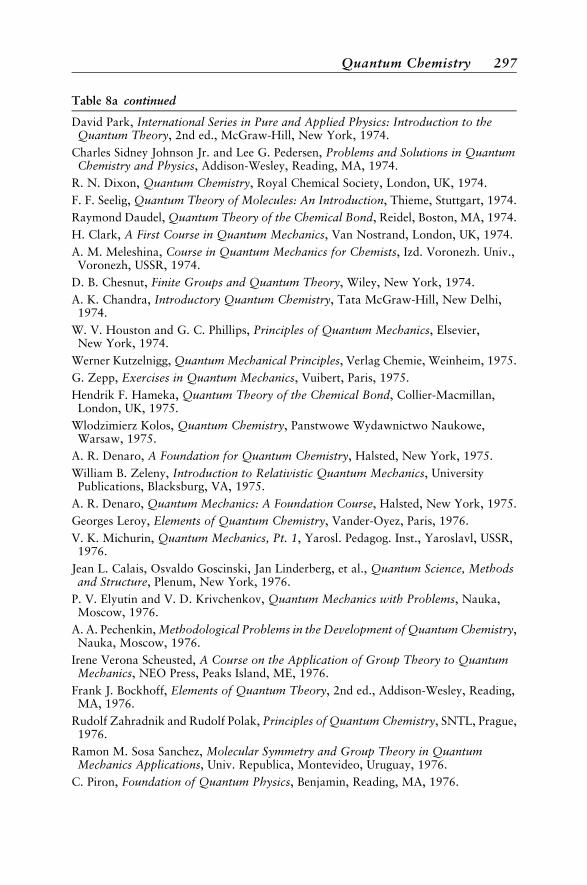
Table 8a continued

David Park, International Series in Pure and Applied Physics: Introduction to theQuantum Theory, 2nd ed., McGraw-Hill, New York, 1974.

Charles Sidney Johnson Jr. and Lee G. Pedersen, Problems and Solutions in QuantumChemistry and Physics, Addison-Wesley, Reading, MA, 1974.

R. N. Dixon, Quantum Chemistry, Royal Chemical Society, London, UK, 1974.

F. F. Seelig, Quantum Theory of Molecules: An Introduction, Thieme, Stuttgart, 1974.

Raymond Daudel, Quantum Theory of the Chemical Bond, Reidel, Boston, MA, 1974.

H. Clark, A First Course in Quantum Mechanics, Van Nostrand, London, UK, 1974.

A. M. Meleshina, Course in Quantum Mechanics for Chemists, Izd. Voronezh. Univ.,Voronezh, USSR, 1974.

D. B. Chesnut, Finite Groups and Quantum Theory, Wiley, New York, 1974.

A. K. Chandra, Introductory Quantum Chemistry, Tata McGraw-Hill, New Delhi,1974.

W. V. Houston and G. C. Phillips, Principles of Quantum Mechanics, Elsevier,New York, 1974.

Werner Kutzelnigg, Quantum Mechanical Principles, Verlag Chemie, Weinheim, 1975.

G. Zepp, Exercises in Quantum Mechanics, Vuibert, Paris, 1975.

Hendrik F. Hameka, Quantum Theory of the Chemical Bond, Collier-Macmillan,London, UK, 1975.

Wlodzimierz Kolos, Quantum Chemistry, Panstwowe Wydawnictwo Naukowe,Warsaw, 1975.

A. R. Denaro, A Foundation for Quantum Chemistry, Halsted, New York, 1975.

William B. Zeleny, Introduction to Relativistic Quantum Mechanics, UniversityPublications, Blacksburg, VA, 1975.

A. R. Denaro, Quantum Mechanics: A Foundation Course, Halsted, New York, 1975.

Georges Leroy, Elements of Quantum Chemistry, Vander-Oyez, Paris, 1976.

V. K. Michurin, Quantum Mechanics, Pt. 1, Yarosl. Pedagog. Inst., Yaroslavl, USSR,1976.

Jean L. Calais, Osvaldo Goscinski, Jan Linderberg, et al., Quantum Science, Methodsand Structure, Plenum, New York, 1976.

P. V. Elyutin and V. D. Krivchenkov, Quantum Mechanics with Problems, Nauka,Moscow, 1976.

A. A. Pechenkin, Methodological Problems in the Development of Quantum Chemistry,Nauka, Moscow, 1976.

Irene Verona Scheusted, A Course on the Application of Group Theory to QuantumMechanics, NEO Press, Peaks Island, ME, 1976.

Frank J. Bockhoff, Elements of Quantum Theory, 2nd ed., Addison-Wesley, Reading,MA, 1976.

Rudolf Zahradnik and Rudolf Polak, Principles of Quantum Chemistry, SNTL, Prague,1976.

Ramon M. Sosa Sanchez, Molecular Symmetry and Group Theory in QuantumMechanics Applications, Univ. Republica, Montevideo, Uruguay, 1976.

C. Piron, Foundation of Quantum Physics, Benjamin, Reading, MA, 1976.

Quantum Chemistry 297

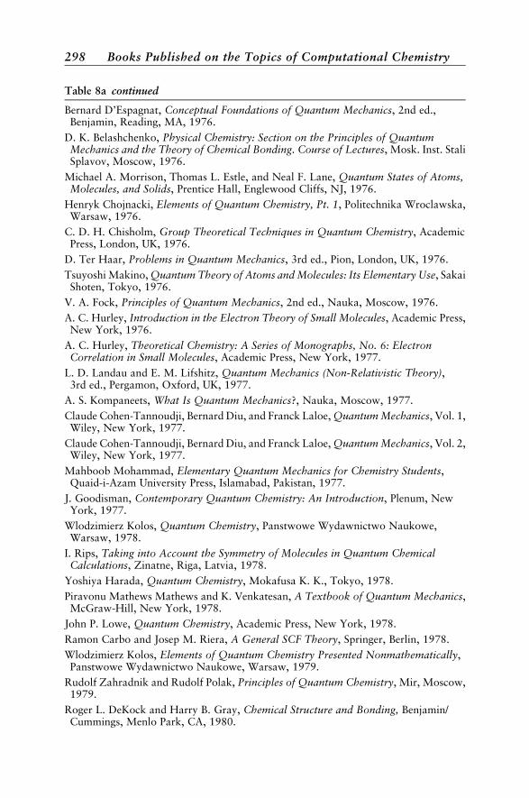
Table 8a continued

Bernard D’Espagnat, Conceptual Foundations of Quantum Mechanics, 2nd ed.,Benjamin, Reading, MA, 1976.

D. K. Belashchenko, Physical Chemistry: Section on the Principles of QuantumMechanics and the Theory of Chemical Bonding. Course of Lectures, Mosk. Inst. StaliSplavov, Moscow, 1976.

Michael A. Morrison, Thomas L. Estle, and Neal F. Lane, Quantum States of Atoms,Molecules, and Solids, Prentice Hall, Englewood Cliffs, NJ, 1976.

Henryk Chojnacki, Elements of Quantum Chemistry, Pt. 1, Politechnika Wroclawska,Warsaw, 1976.

C. D. H. Chisholm, Group Theoretical Techniques in Quantum Chemistry, AcademicPress, London, UK, 1976.

D. Ter Haar, Problems in Quantum Mechanics, 3rd ed., Pion, London, UK, 1976.

Tsuyoshi Makino, Quantum Theory of Atoms and Molecules: Its Elementary Use, SakaiShoten, Tokyo, 1976.

V. A. Fock, Principles of Quantum Mechanics, 2nd ed., Nauka, Moscow, 1976.

A. C. Hurley, Introduction in the Electron Theory of Small Molecules, Academic Press,New York, 1976.

A. C. Hurley, Theoretical Chemistry: A Series of Monographs, No. 6: ElectronCorrelation in Small Molecules, Academic Press, New York, 1977.

L. D. Landau and E. M. Lifshitz, Quantum Mechanics (Non-Relativistic Theory),3rd ed., Pergamon, Oxford, UK, 1977.

A. S. Kompaneets, What Is Quantum Mechanics?, Nauka, Moscow, 1977.

Claude Cohen-Tannoudji, Bernard Diu, and Franck Laloe, Quantum Mechanics, Vol. 1,Wiley, New York, 1977.

Claude Cohen-Tannoudji, Bernard Diu, and Franck Laloe, Quantum Mechanics, Vol. 2,Wiley, New York, 1977.

Mahboob Mohammad, Elementary Quantum Mechanics for Chemistry Students,Quaid-i-Azam University Press, Islamabad, Pakistan, 1977.

J. Goodisman, Contemporary Quantum Chemistry: An Introduction, Plenum, NewYork, 1977.

Wlodzimierz Kolos, Quantum Chemistry, Panstwowe Wydawnictwo Naukowe,Warsaw, 1978.

I. Rips, Taking into Account the Symmetry of Molecules in Quantum ChemicalCalculations, Zinatne, Riga, Latvia, 1978.

Yoshiya Harada, Quantum Chemistry, Mokafusa K. K., Tokyo, 1978.

Piravonu Mathews Mathews and K. Venkatesan, A Textbook of Quantum Mechanics,McGraw-Hill, New York, 1978.

John P. Lowe, Quantum Chemistry, Academic Press, New York, 1978.

Ramon Carbo and Josep M. Riera, A General SCF Theory, Springer, Berlin, 1978.

Wlodzimierz Kolos, Elements of Quantum Chemistry Presented Nonmathematically,Panstwowe Wydawnictwo Naukowe, Warsaw, 1979.

Rudolf Zahradnik and Rudolf Polak, Principles of Quantum Chemistry, Mir, Moscow,1979.

Roger L. DeKock and Harry B. Gray, Chemical Structure and Bonding, Benjamin/Cummings, Menlo Park, CA, 1980.

298 Books Published on the Topics of Computational Chemistry

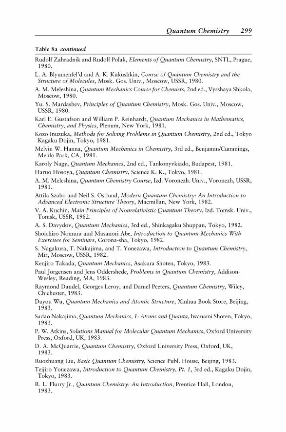
Table 8a continued

Rudolf Zahradnik and Rudolf Polak, Elements of Quantum Chemistry, SNTL, Prague,1980.

L. A. Blyumenfel’d and A. K. Kukushkin, Course of Quantum Chemistry and theStructure of Molecules, Mosk. Gos. Univ., Moscow, USSR, 1980.

A. M. Meleshina, Quantum Mechanics Course for Chemists, 2nd ed., Vysshaya Shkola,Moscow, 1980.

Yu. S. Mardashev, Principles of Quantum Chemistry, Mosk. Gos. Univ., Moscow,USSR, 1980.

Karl E. Gustafson and William P. Reinhardt, Quantum Mechanics in Mathematics,Chemistry, and Physics, Plenum, New York, 1981.

Kozo Inuzuka, Methods for Solving Problems in Quantum Chemistry, 2nd ed., TokyoKagaku Dojin, Tokyo, 1981.

Melvin W. Hanna, Quantum Mechanics in Chemistry, 3rd ed., Benjamin/Cummings,Menlo Park, CA, 1981.

Karoly Nagy, Quantum Mechanics, 2nd ed., Tankonyvkiado, Budapest, 1981.

Haruo Hosoya, Quantum Chemistry, Science K. K., Tokyo, 1981.

A. M. Meleshina, Quantum Chemistry Course, Izd. Voronezh. Univ., Voronezh, USSR,1981.

Attila Szabo and Neil S. Ostlund, Modern Quantum Chemistry: An Introduction toAdvanced Electronic Structure Theory, Macmillan, New York, 1982.

V. A. Kuchin, Main Principles of Nonrelativistic Quantum Theory, Izd. Tomsk. Univ.,Tomsk, USSR, 1982.

A. S. Davydov, Quantum Mechanics, 3rd ed., Shinkagaku Shuppan, Tokyo, 1982.

Shoichiro Nomura and Masanori Abe, Introduction to Quantum Mechanics WithExercises for Seminars, Corona-sha, Tokyo, 1982.

S. Nagakura, T. Nakajima, and T. Yonezawa, Introduction to Quantum Chemistry,Mir, Moscow, USSR, 1982.

Kenjiro Takada, Quantum Mechanics, Asakura Shoten, Tokyo, 1983.

Paul Jorgensen and Jens Oddershede, Problems in Quantum Chemistry, Addison-Wesley, Reading, MA, 1983.

Raymond Daudel, Georges Leroy, and Daniel Peeters, Quantum Chemistry, Wiley,Chichester, 1983.

Dayou Wu, Quantum Mechanics and Atomic Structure, Xinhua Book Store, Beijing,1983.

Sadao Nakajima, Quantum Mechanics, 1: Atoms and Quanta, Iwanami Shoten, Tokyo,1983.

P. W. Atkins, Solutions Manual for Molecular Quantum Mechanics, Oxford UniversityPress, Oxford, UK, 1983.

D. A. McQuarrie, Quantum Chemistry, Oxford University Press, Oxford, UK,1983.

Ruozhuang Liu, Basic Quantum Chemistry, Science Publ. House, Beijing, 1983.

Teijiro Yonezawa, Introduction to Quantum Chemistry, Pt. 1, 3rd ed., Kagaku Dojin,Tokyo, 1983.

R. L. Flurry Jr., Quantum Chemistry: An Introduction, Prentice Hall, London,1983.

Quantum Chemistry 299

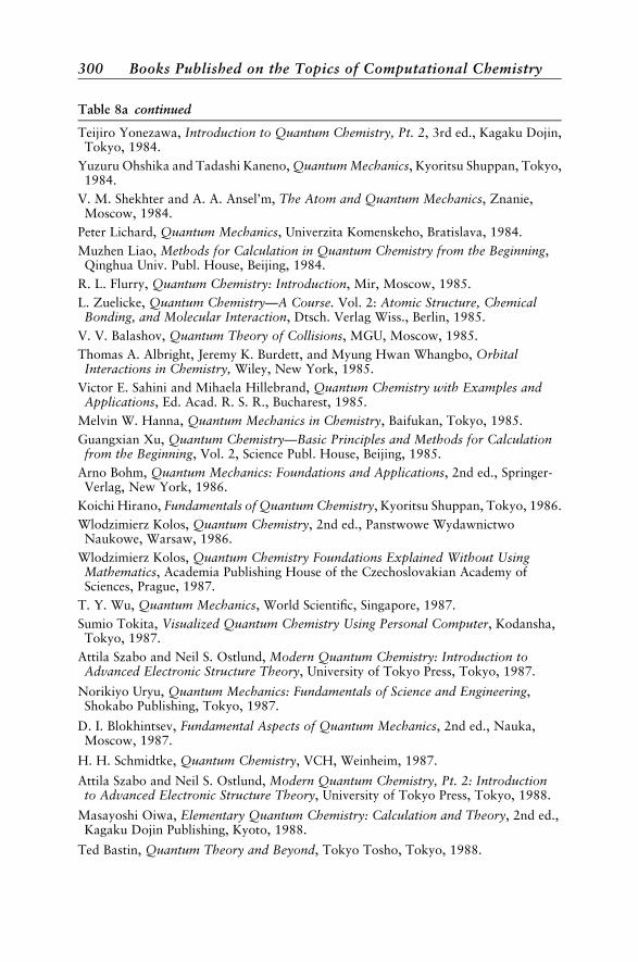
Table 8a continued

Teijiro Yonezawa, Introduction to Quantum Chemistry, Pt. 2, 3rd ed., Kagaku Dojin,Tokyo, 1984.

Yuzuru Ohshika and Tadashi Kaneno, Quantum Mechanics, Kyoritsu Shuppan, Tokyo,1984.

V. M. Shekhter and A. A. Ansel’m, The Atom and Quantum Mechanics, Znanie,Moscow, 1984.

Peter Lichard, Quantum Mechanics, Univerzita Komenskeho, Bratislava, 1984.

Muzhen Liao, Methods for Calculation in Quantum Chemistry from the Beginning,Qinghua Univ. Publ. House, Beijing, 1984.

R. L. Flurry, Quantum Chemistry: Introduction, Mir, Moscow, 1985.

L. Zuelicke, Quantum Chemistry—A Course. Vol. 2: Atomic Structure, ChemicalBonding, and Molecular Interaction, Dtsch. Verlag Wiss., Berlin, 1985.

V. V. Balashov, Quantum Theory of Collisions, MGU, Moscow, 1985.

Thomas A. Albright, Jeremy K. Burdett, and Myung Hwan Whangbo, OrbitalInteractions in Chemistry, Wiley, New York, 1985.

Victor E. Sahini and Mihaela Hillebrand, Quantum Chemistry with Examples andApplications, Ed. Acad. R. S. R., Bucharest, 1985.

Melvin W. Hanna, Quantum Mechanics in Chemistry, Baifukan, Tokyo, 1985.

Guangxian Xu, Quantum Chemistry—Basic Principles and Methods for Calculationfrom the Beginning, Vol. 2, Science Publ. House, Beijing, 1985.

Arno Bohm, Quantum Mechanics: Foundations and Applications, 2nd ed., Springer-Verlag, New York, 1986.

Koichi Hirano, Fundamentals of Quantum Chemistry, Kyoritsu Shuppan, Tokyo, 1986.

Wlodzimierz Kolos, Quantum Chemistry, 2nd ed., Panstwowe WydawnictwoNaukowe, Warsaw, 1986.

Wlodzimierz Kolos, Quantum Chemistry Foundations Explained Without UsingMathematics, Academia Publishing House of the Czechoslovakian Academy ofSciences, Prague, 1987.

T. Y. Wu, Quantum Mechanics, World Scientific, Singapore, 1987.

Sumio Tokita, Visualized Quantum Chemistry Using Personal Computer, Kodansha,Tokyo, 1987.

Attila Szabo and Neil S. Ostlund, Modern Quantum Chemistry: Introduction toAdvanced Electronic Structure Theory, University of Tokyo Press, Tokyo, 1987.

Norikiyo Uryu, Quantum Mechanics: Fundamentals of Science and Engineering,Shokabo Publishing, Tokyo, 1987.

D. I. Blokhintsev, Fundamental Aspects of Quantum Mechanics, 2nd ed., Nauka,Moscow, 1987.

H. H. Schmidtke, Quantum Chemistry, VCH, Weinheim, 1987.

Attila Szabo and Neil S. Ostlund, Modern Quantum Chemistry, Pt. 2: Introductionto Advanced Electronic Structure Theory, University of Tokyo Press, Tokyo, 1988.

Masayoshi Oiwa, Elementary Quantum Chemistry: Calculation and Theory, 2nd ed.,Kagaku Dojin Publishing, Kyoto, 1988.

Ted Bastin, Quantum Theory and Beyond, Tokyo Tosho, Tokyo, 1988.

300 Books Published on the Topics of Computational Chemistry

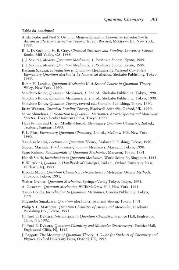
Table 8a continued

Attila Szabo and Neil S. Ostlund, Modern Quantum Chemistry: Introduction toAdvanced Electronic Structure Theory. 1st ed., Revised, McGraw-Hill, New York,1989.

R. L. DeKock and H. B. Gray, Chemical Structure and Bonding, University ScienceBooks, Mill Valley, CA, 1989.

J. J. Sakurai, Modern Quantum Mechanics, 1, Yoshioka Shoten, Kyoto, 1989.

J. J. Sakurai, Modern Quantum Mechanics, 2, Yoshioka Shoten, Kyoto, 1989.

Katsumi Sakurai, Introduction to Quantum Mechanics by Personal Computer:Elementary Quantum Mechanics by Numerical Method, Shokabo Publishing, Tokyo,1989.

Rubin H. Landau, Quantum Mechanics II. A Second Course in Quantum Theory,Wiley, New York, 1990.

Shoichiro Koide, Quantum Mechanics, 1, 2nd ed., Shokabo Publishing, Tokyo, 1990.

Shoichiro Koide, Quantum Mechanics, 2, 2nd ed., Shokabo Publishing, Tokyo, 1990.

Shoichiro Koide, Quantum Theory, revised ed., Shokabo Publishing, Tokyo, 1990.

Brian Webster, Chemical Bonding Theory, Blackwell Scientific, Oxford, UK, 1990.

Shozo Shinohara, Introduction to Quantum Mechanics: Atomic Spectra and MolecularSpectra, Tokyo Denki University Press, Tokyo, 1990.

Hans Primas and Ulrich Mueller-Herold, Elementary Quantum Chemistry, 2nd ed.,Teubner, Stuttgart, 1990.

F. L. Pilar, Elementary Quantum Chemistry, 2nd ed., McGraw-Hill, New York1990.

Yasuhisa Murai, Lectures on Quantum Theory, Asakura Publishing, Tokyo, 1990.

Shigeru Machida, Fundamental Quantum Mechanics, Maruzen, Tokyo, 1990.

Seigo Kishino, Fundamentals of Quantum Mechanics, Maruzen, Tokyo, 1991.

Henrik Smith, Introduction to Quantum Mechanics, World Scientific, Singapore, 1991.

P. W. Atkins, Quanta: A Handbook of Concepts, 2nd ed., Oxford University Press,Fairlawn, NJ, 1991.

Kiyoshi Mutai, Quantum Chemistry: Introduction to Molecular Orbital Methods,Shokodo, Tokyo, 1991.

Walter Greiner, Quantum Mechanics, Springer-Verlag Tokyo, Tokyo, 1991.

A. Goswami, Quantum Mechanics, WCB/McGraw-Hill, New York, 1991.

Yasuo Gondo, Introduction to Quantum Mechanics, Corona Publishing, Tokyo,1991.

Shigenobu Sunakawa, Quantum Mechanics, Iwanami Shoten, Tokyo, 1991.

Philip S. C. Matthews, Quantum Chemistry of Atoms and Molecules, HirokawaPublishing Co., Tokyo, 1991.

Clifford E. Dykstra, Introduction to Quantum Chemistry, Prentice Hall, EnglewoodCliffs, NJ, 1992.

Clifford E. Dykstra, Quantum Chemistry and Molecular Spectroscopy, Prentice Hall,Englewood Cliffs, NJ, 1992.

J. Baggott, The Meaning of Quantum Theory: A Guide for Students of Chemistry andPhysics, Oxford University Press, Oxford, UK, 1992.

Quantum Chemistry 301

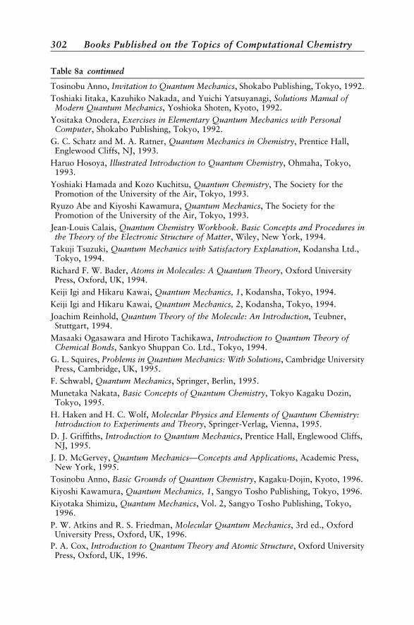
Table 8a continued

Tosinobu Anno, Invitation to Quantum Mechanics, Shokabo Publishing, Tokyo, 1992.

Toshiaki Iitaka, Kazuhiko Nakada, and Yuichi Yatsuyanagi, Solutions Manual ofModern Quantum Mechanics, Yoshioka Shoten, Kyoto, 1992.

Yositaka Onodera, Exercises in Elementary Quantum Mechanics with PersonalComputer, Shokabo Publishing, Tokyo, 1992.

G. C. Schatz and M. A. Ratner, Quantum Mechanics in Chemistry, Prentice Hall,Englewood Cliffs, NJ, 1993.

Haruo Hosoya, Illustrated Introduction to Quantum Chemistry, Ohmaha, Tokyo,1993.

Yoshiaki Hamada and Kozo Kuchitsu, Quantum Chemistry, The Society for thePromotion of the University of the Air, Tokyo, 1993.

Ryuzo Abe and Kiyoshi Kawamura, Quantum Mechanics, The Society for thePromotion of the University of the Air, Tokyo, 1993.

Jean-Louis Calais, Quantum Chemistry Workbook. Basic Concepts and Procedures inthe Theory of the Electronic Structure of Matter, Wiley, New York, 1994.

Takuji Tsuzuki, Quantum Mechanics with Satisfactory Explanation, Kodansha Ltd.,Tokyo, 1994.

Richard F. W. Bader, Atoms in Molecules: A Quantum Theory, Oxford UniversityPress, Oxford, UK, 1994.

Keiji Igi and Hikaru Kawai, Quantum Mechanics, 1, Kodansha, Tokyo, 1994.

Keiji Igi and Hikaru Kawai, Quantum Mechanics, 2, Kodansha, Tokyo, 1994.

Joachim Reinhold, Quantum Theory of the Molecule: An Introduction, Teubner,Stuttgart, 1994.

Masaaki Ogasawara and Hiroto Tachikawa, Introduction to Quantum Theory ofChemical Bonds, Sankyo Shuppan Co. Ltd., Tokyo, 1994.

G. L. Squires, Problems in Quantum Mechanics: With Solutions, Cambridge UniversityPress, Cambridge, UK, 1995.

F. Schwabl, Quantum Mechanics, Springer, Berlin, 1995.

Munetaka Nakata, Basic Concepts of Quantum Chemistry, Tokyo Kagaku Dozin,Tokyo, 1995.

H. Haken and H. C. Wolf, Molecular Physics and Elements of Quantum Chemistry:Introduction to Experiments and Theory, Springer-Verlag, Vienna, 1995.

D. J. Griffiths, Introduction to Quantum Mechanics, Prentice Hall, Englewood Cliffs,NJ, 1995.

J. D. McGervey, Quantum Mechanics—Concepts and Applications, Academic Press,New York, 1995.

Tosinobu Anno, Basic Grounds of Quantum Chemistry, Kagaku-Dojin, Kyoto, 1996.

Kiyoshi Kawamura, Quantum Mechanics, 1, Sangyo Tosho Publishing, Tokyo, 1996.

Kiyotaka Shimizu, Quantum Mechanics, Vol. 2, Sangyo Tosho Publishing, Tokyo,1996.

P. W. Atkins and R. S. Friedman, Molecular Quantum Mechanics, 3rd ed., OxfordUniversity Press, Oxford, UK, 1996.

P. A. Cox, Introduction to Quantum Theory and Atomic Structure, Oxford UniversityPress, Oxford, UK, 1996.

302 Books Published on the Topics of Computational Chemistry

Table 8a continued

Kenichiro Nakamura, Fundamentals of Quantum Physical Chemistry, Tokai UniversityPress, Tokyo, 1996.

Yoshimasa Murayama, Koji Kajita, Kenji Makoshi, et al., Quantum Mechanics,Baifukan, Tokyo, 1996.

Masanori Abe, Quantum Chemistry for Beginners, Baifukan, Tokyo, 1996.

Leslie E. Ballentine, Quantum Mechanics: A Modern Development, World Scientific,Singapore, 1996.

Takashi Fujikawa, Introduction to Schroedinger Equation and Its Applications,Shokabo Publishing, Tokyo, 1996.

Krishnan Balasubramanian, Relativistic Effects in Chemistry, Part A: Theory andTechniques and Relativistic Effects in Chemistry, Wiley, New York, 1997.

Krishnan Balasubramanian, Relativistic Effects in Chemistry, Part B: Applications,Wiley, New York, 1997.

Jack Simons and Jeff Nichols, Quantum Mechanics in Chemistry, Oxford UniversityPress, New York, 1997.

Hinne Hettema, Quantum Chemistry: Classic Scientific Papers, World Scientific,Singapore, 1997.

Jean-Louis Calais and Eugene Kryachko, Conceptual Perspectives in QuantumChemistry, Kluwer, Dordrecht, 1997.

N. J. B. Green, Quantum Mechanics 1. Foundations, Oxford University Press, Oxford,UK, 1997.

J. E. House, Fundamental of Quantum Mechanics, Academic Press, New York, 1998.

Nicholass Green, Quantum Mechanics 2: The Toolkit, Oxford University Press,Oxford, UK, 1998.

Ira N. Levine, Quantum Chemistry, 5th ed., Prentice Hall, Englewood Cliffs, NJ,1998.

Per-Olov Lowdin, Linear Algebra for Quantum Theory, Wiley, New York, 1998.

K. Hirao, Recent Advances in Multireference Methods, Vol. 4, World Scientific,Singapore, 1999.

Peter R. Surjan, Correlation and Localization, Top. Curr. Chem., 203, Springer, Berlin,1999.

Rudolf Haussmann, Self-Consistent Field Theory and Bosonization for StronglyCorrelated Electron Systems, Springer, Berlin, 1999.

Wolfram Koch and Max C. Holthausen, A Chemist’s Guide to Density FunctionalTheory, Wiley-VCH, Weinheim, 2000.

Ruben Pauncz, The Construction of Spin Eigenfunctions. An Exercise Book, KluwerAcademic/Plenum Publishers, Dordrecht, 2000.

Tamas Veszpremi and Miklos Feher, Quantum Chemistry. Fundamentals to Applica-tions, Kluwer Academic/Plenum Publishers, Dordrecht, 2000.

Stephen Wilson, An Introduction to the Methods of Relativistic Molecular QuantumMechanics, World Scientific, Singapore, 2000.

Trygve Helgaker, Poul Jorgensen, and Jeppe Olsen, Molecular Electronic-StructureTheory, Wiley, New York, 2000.

Quantum Chemistry 303

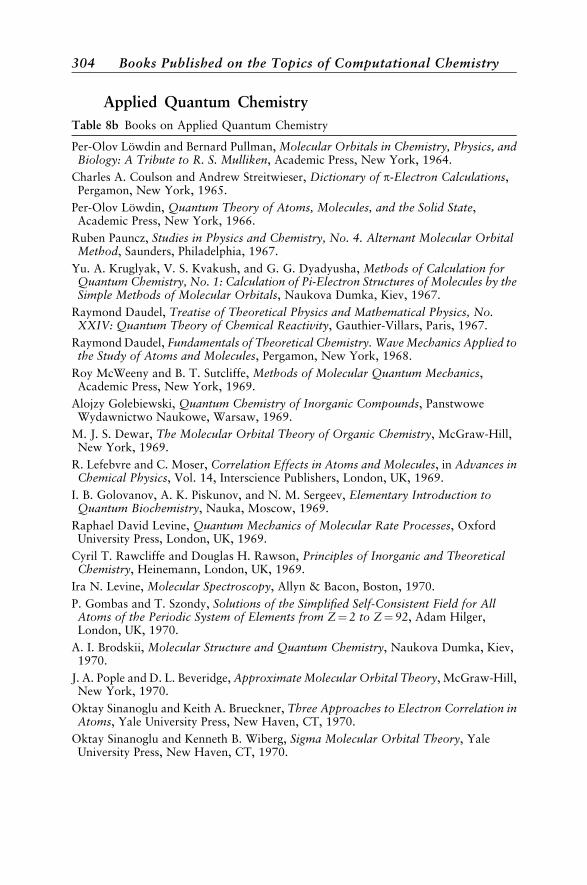
Applied Quantum Chemistry

Table 8b Books on Applied Quantum Chemistry

Per-Olov Lowdin and Bernard Pullman, Molecular Orbitals in Chemistry, Physics, andBiology: A Tribute to R. S. Mulliken, Academic Press, New York, 1964.

Charles A. Coulson and Andrew Streitwieser, Dictionary of p-Electron Calculations,Pergamon, New York, 1965.

Per-Olov Lowdin, Quantum Theory of Atoms, Molecules, and the Solid State,Academic Press, New York, 1966.

Ruben Pauncz, Studies in Physics and Chemistry, No. 4. Alternant Molecular OrbitalMethod, Saunders, Philadelphia, 1967.

Yu. A. Kruglyak, V. S. Kvakush, and G. G. Dyadyusha, Methods of Calculation forQuantum Chemistry, No. 1: Calculation of Pi-Electron Structures of Molecules by theSimple Methods of Molecular Orbitals, Naukova Dumka, Kiev, 1967.

Raymond Daudel, Treatise of Theoretical Physics and Mathematical Physics, No.XXIV: Quantum Theory of Chemical Reactivity, Gauthier-Villars, Paris, 1967.

Raymond Daudel, Fundamentals of Theoretical Chemistry. Wave Mechanics Applied tothe Study of Atoms and Molecules, Pergamon, New York, 1968.

Roy McWeeny and B. T. Sutcliffe, Methods of Molecular Quantum Mechanics,Academic Press, New York, 1969.

Alojzy Golebiewski, Quantum Chemistry of Inorganic Compounds, PanstwoweWydawnictwo Naukowe, Warsaw, 1969.

M. J. S. Dewar, The Molecular Orbital Theory of Organic Chemistry, McGraw-Hill,New York, 1969.

R. Lefebvre and C. Moser, Correlation Effects in Atoms and Molecules, in Advances inChemical Physics, Vol. 14, Interscience Publishers, London, UK, 1969.

I. B. Golovanov, A. K. Piskunov, and N. M. Sergeev, Elementary Introduction toQuantum Biochemistry, Nauka, Moscow, 1969.

Raphael David Levine, Quantum Mechanics of Molecular Rate Processes, OxfordUniversity Press, London, UK, 1969.

Cyril T. Rawcliffe and Douglas H. Rawson, Principles of Inorganic and TheoreticalChemistry, Heinemann, London, UK, 1969.

Ira N. Levine, Molecular Spectroscopy, Allyn & Bacon, Boston, 1970.

P. Gombas and T. Szondy, Solutions of the Simplified Self-Consistent Field for AllAtoms of the Periodic System of Elements from Z¼ 2 to Z¼ 92, Adam Hilger,London, UK, 1970.

A. I. Brodskii, Molecular Structure and Quantum Chemistry, Naukova Dumka, Kiev,1970.

J. A. Pople and D. L. Beveridge, Approximate Molecular Orbital Theory, McGraw-Hill,New York, 1970.

Oktay Sinanoglu and Keith A. Brueckner, Three Approaches to Electron Correlation inAtoms, Yale University Press, New Haven, CT, 1970.

Oktay Sinanoglu and Kenneth B. Wiberg, Sigma Molecular Orbital Theory, YaleUniversity Press, New Haven, CT, 1970.

304 Books Published on the Topics of Computational Chemistry

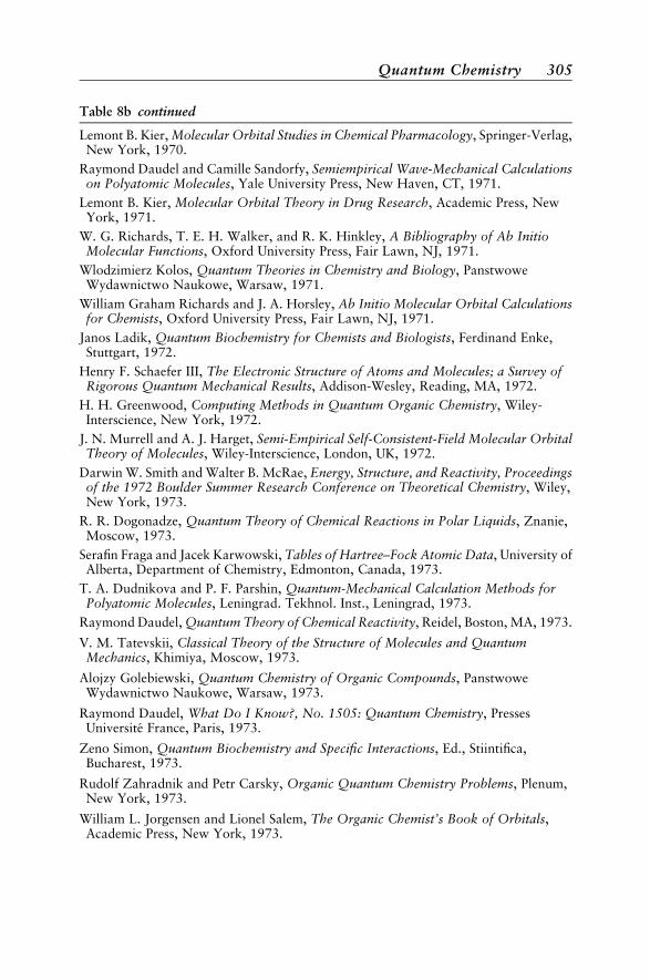
Table 8b continued

Lemont B. Kier, Molecular Orbital Studies in Chemical Pharmacology, Springer-Verlag,New York, 1970.

Raymond Daudel and Camille Sandorfy, Semiempirical Wave-Mechanical Calculationson Polyatomic Molecules, Yale University Press, New Haven, CT, 1971.

Lemont B. Kier, Molecular Orbital Theory in Drug Research, Academic Press, NewYork, 1971.

W. G. Richards, T. E. H. Walker, and R. K. Hinkley, A Bibliography of Ab InitioMolecular Functions, Oxford University Press, Fair Lawn, NJ, 1971.

Wlodzimierz Kolos, Quantum Theories in Chemistry and Biology, PanstwoweWydawnictwo Naukowe, Warsaw, 1971.

William Graham Richards and J. A. Horsley, Ab Initio Molecular Orbital Calculationsfor Chemists, Oxford University Press, Fair Lawn, NJ, 1971.

Janos Ladik, Quantum Biochemistry for Chemists and Biologists, Ferdinand Enke,Stuttgart, 1972.

Henry F. Schaefer III, The Electronic Structure of Atoms and Molecules; a Survey ofRigorous Quantum Mechanical Results, Addison-Wesley, Reading, MA, 1972.

H. H. Greenwood, Computing Methods in Quantum Organic Chemistry, Wiley-Interscience, New York, 1972.

J. N. Murrell and A. J. Harget, Semi-Empirical Self-Consistent-Field Molecular OrbitalTheory of Molecules, Wiley-Interscience, London, UK, 1972.

Darwin W. Smith and Walter B. McRae, Energy, Structure, and Reactivity, Proceedingsof the 1972 Boulder Summer Research Conference on Theoretical Chemistry, Wiley,New York, 1973.

R. R. Dogonadze, Quantum Theory of Chemical Reactions in Polar Liquids, Znanie,Moscow, 1973.

Serafin Fraga and Jacek Karwowski, Tables of Hartree–Fock Atomic Data, University ofAlberta, Department of Chemistry, Edmonton, Canada, 1973.

T. A. Dudnikova and P. F. Parshin, Quantum-Mechanical Calculation Methods forPolyatomic Molecules, Leningrad. Tekhnol. Inst., Leningrad, 1973.

Raymond Daudel, Quantum Theory of Chemical Reactivity, Reidel, Boston, MA, 1973.

V. M. Tatevskii, Classical Theory of the Structure of Molecules and QuantumMechanics, Khimiya, Moscow, 1973.

Alojzy Golebiewski, Quantum Chemistry of Organic Compounds, PanstwoweWydawnictwo Naukowe, Warsaw, 1973.

Raymond Daudel, What Do I Know?, No. 1505: Quantum Chemistry, PressesUniversite France, Paris, 1973.

Zeno Simon, Quantum Biochemistry and Specific Interactions, Ed., Stiintifica,Bucharest, 1973.

Rudolf Zahradnik and Petr Carsky, Organic Quantum Chemistry Problems, Plenum,New York, 1973.

William L. Jorgensen and Lionel Salem, The Organic Chemist’s Book of Orbitals,Academic Press, New York, 1973.

Quantum Chemistry 305

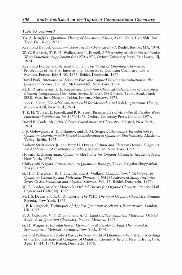
Table 8b continued

Yu. A. Kruglyak, Quantum Theory of Solvation of Ions, Akad. Nauk Ukr. SSR, Inst.Teor. Fiz., Kiev, 1973.

Raymond Daudel, Quantum Theory of the Chemical Bond, Reidel, Boston, MA, 1974.

W. G. Richards, T. E. H. Walker, and L. Farnell, Bibliography of Ab Initio MolecularWave Functions: Supplement for 1970–1973, Oxford University Press, Fair Lawn, NJ,1974.

Raymond Daudel and Bernard Pullman, The World of Quantum Chemistry,Proceedings of the First International Congress of Quantum Chemistry held atMenton, France, July 4–10, 1973, Reidel, Dordrecht, 1974.

David Park, International Series in Pure and Applied Physics: Introduction to theQuantum Theory, 2nd ed., McGraw-Hill, New York, 1974.

M. E. Dyatkina and E. L. Rozenberg, Quantum Chemical Calculations of TransitionElement Compounds, Gos. Kom. Soveta Ministr. SSSR Nauk. Tekh., Acad. NaukSSSR, Vses. Inst. Nauchn. Tekhn. Inform., Moscow, 1974.

John C. Slater, The Self-Consistent Field for Molecules and Solids. Quantum Theory,McGraw-Hill, New York, 1974.

T. E. H. Walker, L. Farnell, and P. R. Scott, Bibliography of Ab Initio Molecular WaveFunctions: Supplement for 1970–1973, Oxford University Press, London, 1974.

David B. Cook, Ab Initio Valence Calculations in Chemistry, Halsted, New York,1974.

I. B. Golowanov, A. K. Piskunov, and N. M. Sergeev, Elementary Introduction toQuantum Chemistry with Special Consideration of Quantum Biochemistry, AkademicVerlag, Berlin, 1975.

Andrew Streitwieser Jr. and Peter H. Owens, Orbital and Electron Density Diagrams:An Application of Computer Graphics, Macmillan, New York, 1975.

Howard E. Zimmerman, Quantum Mechanics for Organic Chemists, Academic Press,New York, 1975.

Chikayoshi Nagata, Introduction to Quantum Biology, Tokyo Daigaku Shuppankai,Tokyo, 1975.

G. H. F. Diercksen, B. T. Sutcliffe, and A. Veillard, Computational Techniques inQuantum Chemistry and Molecular Physics, in NATO Advanced Study InstitutesSeries C: Mathematical and Physical Sciences, Vol. 15, Reidel, Dordrecht, 1975.

W. T. Borden, Modern Molecular Orbital Theory for Organic Chemists, Prentice Hall,Englewood Cliffs, NJ, 1975.

M. J. S. Dewar and R. C. Dougherty, The PMO Theory of Organic Chemistry, Plenum/Rosetta, New York, 1975.

J. P. Killingbeck, Techniques of Applied Quantum Mechanics, Butterworth, London,UK, 1975.

V. A. Gubanov, V. P. Zhukov, and A. O. Litinskii, Semiempirical Molecular OrbitalMethods in Quantum Chemistry, Nauka, Moscow, 1976.

G. H. Wagniere, Introduction to Elementary Molecular Orbital Theory and toSemiempirical Methods, Springer, New York, 1976.

Bernard Pullman and Robert Parr, The New World of Quantum Chemistry, Proceedingsof the 2nd International Congress of Quantum Chemistry held at New Orleans, USA,April 19–24, 1976, Reidel, Dordrecht, 1976.

306 Books Published on the Topics of Computational Chemistry

Table 8b continued

E. R. Davidson, Reduced Density Matrixes in Quantum Chemistry, Academic Press,New York, 1976.

D. A. Zhogolev and V. B. Volkov, Methods, Algorithms, and Programs for Quantum-Chemical Calculations for Molecules, Naukova Dumka, Kiev, 1976.

G. Berthier, M. J. S. Dewar, and H. Fischer, Introduction to Elementary MolecularOrbital Theory and to Semiempirical Methods, in Lecture Notes in Chemistry, Vol. 1,Springer, Berlin, 1976.

R. McWeeny and B. T. Sutcliffe, Methods of Molecular Quantum Mechanics, 2nd ed.,Academic Press, London, UK, 1976.

Bernard Pullman, Perspectives in Quantum Chemistry and Biochemistry: QuantumMechanics of Molecular Conformations, Wiley, Chichester, 1976.

Joanna Sadlej, Semiempirical Methods of CNDO, INDO, and NDDO QuantumChemistry, Panstwowe Wydawnictwo Naukowe, Warsaw, 1977.

A. B. Migdal, Qualitative Methods in Quantum Theory, Benjamin, Reading, MA,1977.

H. F. Schaefer III, Methods of Electronic Structure Theory, Plenum, New York, 1977.

J. A. Pople, H. G. Drickamer, and F. H. Stillinger, Symposium on Structure andQuantum Chemistry and Symposium on Evolution of Magnetic Resonance, AmericanChemical Society, Washington, DC, 1977.

W. G. Richards, Quantum Pharmacology, Butterworth, London, UK, 1977.

Gerald A. Segal, Semiempirical Methods of Electronic Structure Calculation, Pt. A:Techniques, in Modern Theoretical Chemistry, Vol. 7, Plenum, New York, 1977.

Mark A. Ratner, John R. Sabin, and Samuel B. Trickey, Applications of ModelHamiltonians to the Electron Dynamics of Organic Charge Transfer Salts inUncertainty Princ. Found. Quantum Mech., William Charles Price and Seymour S.Chissick, Eds., Wiley, Chichester, 1977.

Gerald A. Segal, Semiempirical Methods of Electronic Structure Calculation: Applica-tions, in Modern Theoretical Chemistry, Vol. 8, Pt. B, Plenum, New York, 1977.

Charlotte Froese Fischer, The Hartree–Fock Method for Atoms: A NumericalApproach, Wiley, New York, 1977.

M. M. Mestechkin, Density Matrix Method in the Theory of Molecules, NaukovaDumka, Kiev, 1977.

L. N. Petrov and V. O. Reisfel’d, Quantum-Chemical Calculations, Leningr. Tekhnol.Inst., Leningrad, 1977.

C. F. Fischer, The Hartree–Fock Method for Atoms: A Numerical Approach, Wiley,New York, 1977.

John C. Slater, The Self-Consistent Field for Molecules and Solids, Mir, Moscow,1978.

N. M. Klimenko, Quantum Chemical Calculations of Transition Metal Complexes,VINITI, Moscow, 1978.

D. H. Whitten, IUPAC Physical Chemistry Division. Expression of Results in QuantumChemistry, Pergamon, Oxford, UK, 1978.

Bernard Pullman, Intermolecular Interactions: From Diatomics to Biopolymers, inPerspectives in Quantum Chemistry and Biochemistry, Vol. 2, Wiley, Chichester,1978.

Quantum Chemistry 307

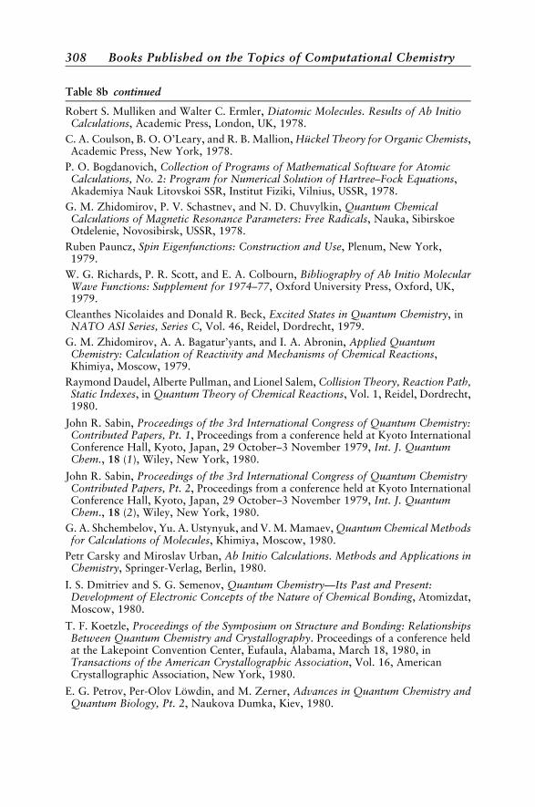
Table 8b continued

Robert S. Mulliken and Walter C. Ermler, Diatomic Molecules. Results of Ab InitioCalculations, Academic Press, London, UK, 1978.

C. A. Coulson, B. O. O’Leary, and R. B. Mallion, Huckel Theory for Organic Chemists,Academic Press, New York, 1978.

P. O. Bogdanovich, Collection of Programs of Mathematical Software for AtomicCalculations, No. 2: Program for Numerical Solution of Hartree–Fock Equations,Akademiya Nauk Litovskoi SSR, Institut Fiziki, Vilnius, USSR, 1978.

G. M. Zhidomirov, P. V. Schastnev, and N. D. Chuvylkin, Quantum ChemicalCalculations of Magnetic Resonance Parameters: Free Radicals, Nauka, SibirskoeOtdelenie, Novosibirsk, USSR, 1978.

Ruben Pauncz, Spin Eigenfunctions: Construction and Use, Plenum, New York,1979.

W. G. Richards, P. R. Scott, and E. A. Colbourn, Bibliography of Ab Initio MolecularWave Functions: Supplement for 1974–77, Oxford University Press, Oxford, UK,1979.

Cleanthes Nicolaides and Donald R. Beck, Excited States in Quantum Chemistry, inNATO ASI Series, Series C, Vol. 46, Reidel, Dordrecht, 1979.

G. M. Zhidomirov, A. A. Bagatur’yants, and I. A. Abronin, Applied QuantumChemistry: Calculation of Reactivity and Mechanisms of Chemical Reactions,Khimiya, Moscow, 1979.

Raymond Daudel, Alberte Pullman, and Lionel Salem, Collision Theory, Reaction Path,Static Indexes, in Quantum Theory of Chemical Reactions, Vol. 1, Reidel, Dordrecht,1980.

John R. Sabin, Proceedings of the 3rd International Congress of Quantum Chemistry:Contributed Papers, Pt. 1, Proceedings from a conference held at Kyoto InternationalConference Hall, Kyoto, Japan, 29 October–3 November 1979, Int. J. QuantumChem., 18 (1), Wiley, New York, 1980.

John R. Sabin, Proceedings of the 3rd International Congress of Quantum ChemistryContributed Papers, Pt. 2, Proceedings from a conference held at Kyoto InternationalConference Hall, Kyoto, Japan, 29 October–3 November 1979, Int. J. QuantumChem., 18 (2), Wiley, New York, 1980.

G. A. Shchembelov, Yu. A. Ustynyuk, and V. M. Mamaev, Quantum Chemical Methodsfor Calculations of Molecules, Khimiya, Moscow, 1980.

Petr Carsky and Miroslav Urban, Ab Initio Calculations. Methods and Applications inChemistry, Springer-Verlag, Berlin, 1980.

I. S. Dmitriev and S. G. Semenov, Quantum Chemistry—Its Past and Present:Development of Electronic Concepts of the Nature of Chemical Bonding, Atomizdat,Moscow, 1980.

T. F. Koetzle, Proceedings of the Symposium on Structure and Bonding: RelationshipsBetween Quantum Chemistry and Crystallography. Proceedings of a conference heldat the Lakepoint Convention Center, Eufaula, Alabama, March 18, 1980, inTransactions of the American Crystallographic Association, Vol. 16, AmericanCrystallographic Association, New York, 1980.

E. G. Petrov, Per-Olov Lowdin, and M. Zerner, Advances in Quantum Chemistry andQuantum Biology, Pt. 2, Naukova Dumka, Kiev, 1980.

308 Books Published on the Topics of Computational Chemistry

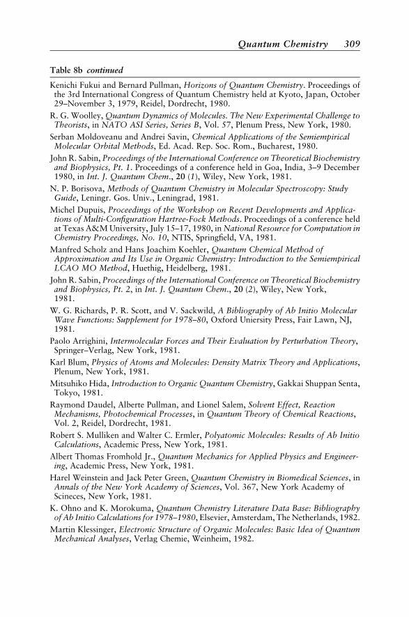
Table 8b continued

Kenichi Fukui and Bernard Pullman, Horizons of Quantum Chemistry. Proceedings ofthe 3rd International Congress of Quantum Chemistry held at Kyoto, Japan, October29–November 3, 1979, Reidel, Dordrecht, 1980.

R. G. Woolley, Quantum Dynamics of Molecules. The New Experimental Challenge toTheorists, in NATO ASI Series, Series B, Vol. 57, Plenum Press, New York, 1980.

Serban Moldoveanu and Andrei Savin, Chemical Applications of the SemiempiricalMolecular Orbital Methods, Ed. Acad. Rep. Soc. Rom., Bucharest, 1980.

John R. Sabin, Proceedings of the International Conference on Theoretical Biochemistryand Biophysics, Pt. 1. Proceedings of a conference held in Goa, India, 3–9 December1980, in Int. J. Quantum Chem., 20 (1), Wiley, New York, 1981.

N. P. Borisova, Methods of Quantum Chemistry in Molecular Spectroscopy: StudyGuide, Leningr. Gos. Univ., Leningrad, 1981.

Michel Dupuis, Proceedings of the Workshop on Recent Developments and Applica-tions of Multi-Configuration Hartree-Fock Methods. Proceedings of a conference heldat Texas A&M University, July 15–17, 1980, in National Resource for Computation inChemistry Proceedings, No. 10, NTIS, Springfield, VA, 1981.

Manfred Scholz and Hans Joachim Koehler, Quantum Chemical Method ofApproximation and Its Use in Organic Chemistry: Introduction to the SemiempiricalLCAO MO Method, Huethig, Heidelberg, 1981.

John R. Sabin, Proceedings of the International Conference on Theoretical Biochemistryand Biophysics, Pt. 2, in Int. J. Quantum Chem., 20 (2), Wiley, New York,1981.

W. G. Richards, P. R. Scott, and V. Sackwild, A Bibliography of Ab Initio MolecularWave Functions: Supplement for 1978–80, Oxford Uniersity Press, Fair Lawn, NJ,1981.

Paolo Arrighini, Intermolecular Forces and Their Evaluation by Perturbation Theory,Springer–Verlag, New York, 1981.

Karl Blum, Physics of Atoms and Molecules: Density Matrix Theory and Applications,Plenum, New York, 1981.

Mitsuhiko Hida, Introduction to Organic Quantum Chemistry, Gakkai Shuppan Senta,Tokyo, 1981.

Raymond Daudel, Alberte Pullman, and Lionel Salem, Solvent Effect, ReactionMechanisms, Photochemical Processes, in Quantum Theory of Chemical Reactions,Vol. 2, Reidel, Dordrecht, 1981.

Robert S. Mulliken and Walter C. Ermler, Polyatomic Molecules: Results of Ab InitioCalculations, Academic Press, New York, 1981.

Albert Thomas Fromhold Jr., Quantum Mechanics for Applied Physics and Engineer-ing, Academic Press, New York, 1981.

Harel Weinstein and Jack Peter Green, Quantum Chemistry in Biomedical Sciences, inAnnals of the New York Academy of Sciences, Vol. 367, New York Academy ofScineces, New York, 1981.

K. Ohno and K. Morokuma, Quantum Chemistry Literature Data Base: Bibliographyof Ab Initio Calculations for 1978–1980, Elsevier, Amsterdam, The Netherlands, 1982.

Martin Klessinger, Electronic Structure of Organic Molecules: Basic Idea of QuantumMechanical Analyses, Verlag Chemie, Weinheim, 1982.

Quantum Chemistry 309

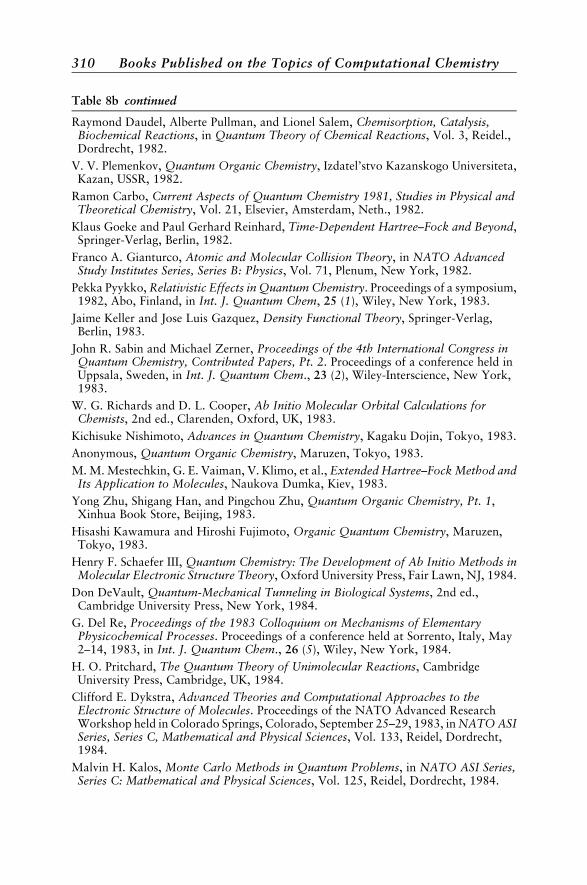
Table 8b continued

Raymond Daudel, Alberte Pullman, and Lionel Salem, Chemisorption, Catalysis,Biochemical Reactions, in Quantum Theory of Chemical Reactions, Vol. 3, Reidel.,Dordrecht, 1982.

V. V. Plemenkov, Quantum Organic Chemistry, Izdatel’stvo Kazanskogo Universiteta,Kazan, USSR, 1982.

Ramon Carbo, Current Aspects of Quantum Chemistry 1981, Studies in Physical andTheoretical Chemistry, Vol. 21, Elsevier, Amsterdam, Neth., 1982.

Klaus Goeke and Paul Gerhard Reinhard, Time-Dependent Hartree–Fock and Beyond,Springer-Verlag, Berlin, 1982.

Franco A. Gianturco, Atomic and Molecular Collision Theory, in NATO AdvancedStudy Institutes Series, Series B: Physics, Vol. 71, Plenum, New York, 1982.

Pekka Pyykko, Relativistic Effects in Quantum Chemistry. Proceedings of a symposium,1982, Abo, Finland, in Int. J. Quantum Chem, 25 (1), Wiley, New York, 1983.

Jaime Keller and Jose Luis Gazquez, Density Functional Theory, Springer-Verlag,Berlin, 1983.

John R. Sabin and Michael Zerner, Proceedings of the 4th International Congress inQuantum Chemistry, Contributed Papers, Pt. 2. Proceedings of a conference held inUppsala, Sweden, in Int. J. Quantum Chem., 23 (2), Wiley-Interscience, New York,1983.

W. G. Richards and D. L. Cooper, Ab Initio Molecular Orbital Calculations forChemists, 2nd ed., Clarenden, Oxford, UK, 1983.

Kichisuke Nishimoto, Advances in Quantum Chemistry, Kagaku Dojin, Tokyo, 1983.

Anonymous, Quantum Organic Chemistry, Maruzen, Tokyo, 1983.

M. M. Mestechkin, G. E. Vaiman, V. Klimo, et al., Extended Hartree–Fock Method andIts Application to Molecules, Naukova Dumka, Kiev, 1983.

Yong Zhu, Shigang Han, and Pingchou Zhu, Quantum Organic Chemistry, Pt. 1,Xinhua Book Store, Beijing, 1983.

Hisashi Kawamura and Hiroshi Fujimoto, Organic Quantum Chemistry, Maruzen,Tokyo, 1983.

Henry F. Schaefer III, Quantum Chemistry: The Development of Ab Initio Methods inMolecular Electronic Structure Theory, Oxford University Press, Fair Lawn, NJ, 1984.

Don DeVault, Quantum-Mechanical Tunneling in Biological Systems, 2nd ed.,Cambridge University Press, New York, 1984.

G. Del Re, Proceedings of the 1983 Colloquium on Mechanisms of ElementaryPhysicochemical Processes. Proceedings of a conference held at Sorrento, Italy, May2–14, 1983, in Int. J. Quantum Chem., 26 (5), Wiley, New York, 1984.

H. O. Pritchard, The Quantum Theory of Unimolecular Reactions, CambridgeUniversity Press, Cambridge, UK, 1984.

Clifford E. Dykstra, Advanced Theories and Computational Approaches to theElectronic Structure of Molecules. Proceedings of the NATO Advanced ResearchWorkshop held in Colorado Springs, Colorado, September 25–29, 1983, in NATO ASISeries, Series C, Mathematical and Physical Sciences, Vol. 133, Reidel, Dordrecht,1984.

Malvin H. Kalos, Monte Carlo Methods in Quantum Problems, in NATO ASI Series,Series C: Mathematical and Physical Sciences, Vol. 125, Reidel, Dordrecht, 1984.

310 Books Published on the Topics of Computational Chemistry

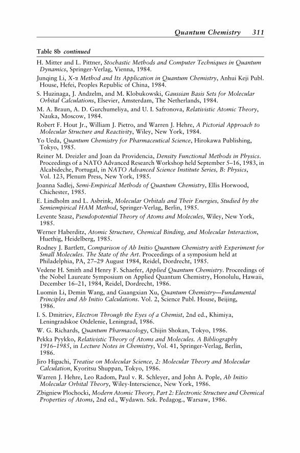
Table 8b continued

H. Mitter and L. Pittner, Stochastic Methods and Computer Techniques in QuantumDynamics, Springer-Verlag, Vienna, 1984.

Junqing Li, X-a Method and Its Application in Quantum Chemistry, Anhui Keji Publ.House, Hefei, Peoples Republic of China, 1984.

S. Huzinaga, J. Andzelm, and M. Klobukowski, Gaussian Basis Sets for MolecularOrbital Calculations, Elsevier, Amsterdam, The Netherlands, 1984.

M. A. Braun, A. D. Gurchumeliya, and U. I. Safronova, Relativistic Atomic Theory,Nauka, Moscow, 1984.

Robert F. Hout Jr., William J. Pietro, and Warren J. Hehre, A Pictorial Approach toMolecular Structure and Reactivity, Wiley, New York, 1984.

Yo Ueda, Quantum Chemistry for Pharmaceutical Science, Hirokawa Publishing,Tokyo, 1985.

Reiner M. Dreizler and Joan da Providencia, Density Functional Methods in Physics.Proceedings of a NATO Advanced Research Workshop held September 5–16, 1983, inAlcabideche, Portugal, in NATO Advanced Science Institute Series, B: Physics,Vol. 123, Plenum Press, New York, 1985.

Joanna Sadlej, Semi-Empirical Methods of Quantum Chemistry, Ellis Horwood,Chichester, 1985.

E. Lindholm and L. Asbrink, Molecular Orbitals and Their Energies, Studied by theSemiempirical HAM Method, Springer-Verlag, Berlin, 1985.

Levente Szasz, Pseudopotential Theory of Atoms and Molecules, Wiley, New York,1985.

Werner Haberditz, Atomic Structure, Chemical Binding, and Molecular Interaction,Huethig, Heidelberg, 1985.

Rodney J. Bartlett, Comparison of Ab Initio Quantum Chemistry with Experiment forSmall Molecules. The State of the Art. Proceedings of a symposium held atPhiladelphia, PA, 27–29 August 1984, Reidel, Dordrecht, 1985.

Vedene H. Smith and Henry F. Schaefer, Applied Quantum Chemistry. Proceedings ofthe Nobel Laureate Symposium on Applied Quantum Chemistry, Honolulu, Hawaii,December 16–21, 1984, Reidel, Dordrecht, 1986.

Luomin Li, Demin Wang, and Guangxian Xu, Quantum Chemistry—FundamentalPrinciples and Ab Initio Calculations. Vol. 2, Science Publ. House, Beijing,1986.

I. S. Dmitriev, Electron Through the Eyes of a Chemist, 2nd ed., Khimiya,Leningradskoe Otdelenie, Leningrad, 1986.

W. G. Richards, Quantum Pharmacology, Chijin Shokan, Tokyo, 1986.

Pekka Pyykko, Relativistic Theory of Atoms and Molecules. A Bibliography1916–1985, in Lecture Notes in Chemistry, Vol. 41, Springer-Verlag, Berlin,1986.

Jiro Higuchi, Treatise on Molecular Science, 2: Molecular Theory and MolecularCalculation, Kyoritsu Shuppan, Tokyo, 1986.

Warren J. Hehre, Leo Radom, Paul v. R. Schleyer, and John A. Pople, Ab InitioMolecular Orbital Theory, Wiley-Interscience, New York, 1986.

Zbigniew Plochocki, Modern Atomic Theory, Part 2: Electronic Structure and ChemicalProperties of Atoms, 2nd ed., Wydawn. Szk. Pedagog., Warsaw, 1986.

Quantum Chemistry 311

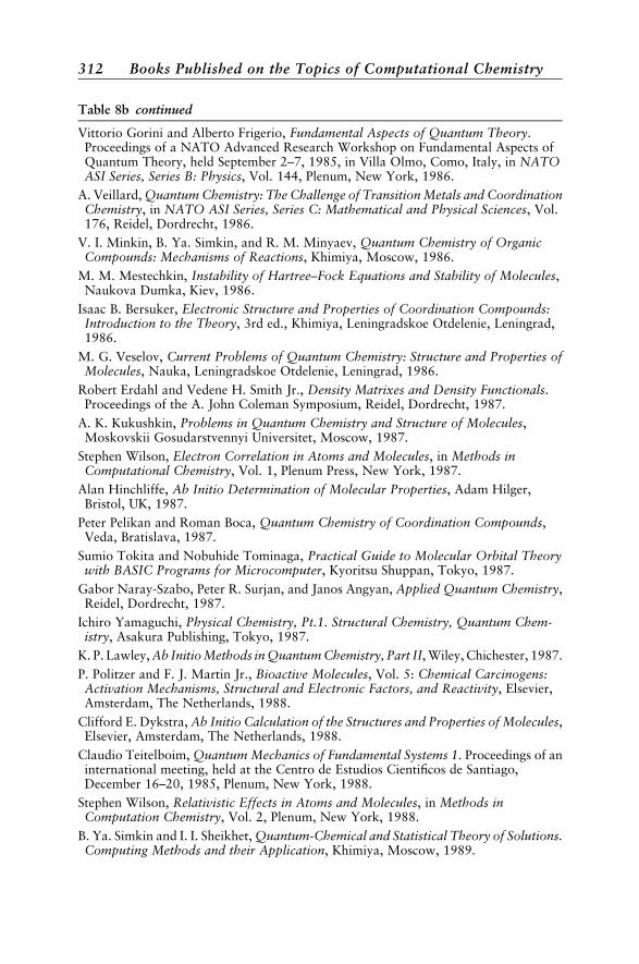
Table 8b continued

Vittorio Gorini and Alberto Frigerio, Fundamental Aspects of Quantum Theory.Proceedings of a NATO Advanced Research Workshop on Fundamental Aspects ofQuantum Theory, held September 2–7, 1985, in Villa Olmo, Como, Italy, in NATOASI Series, Series B: Physics, Vol. 144, Plenum, New York, 1986.

A. Veillard, Quantum Chemistry: The Challenge of Transition Metals and CoordinationChemistry, in NATO ASI Series, Series C: Mathematical and Physical Sciences, Vol.176, Reidel, Dordrecht, 1986.

V. I. Minkin, B. Ya. Simkin, and R. M. Minyaev, Quantum Chemistry of OrganicCompounds: Mechanisms of Reactions, Khimiya, Moscow, 1986.

M. M. Mestechkin, Instability of Hartree–Fock Equations and Stability of Molecules,Naukova Dumka, Kiev, 1986.

Isaac B. Bersuker, Electronic Structure and Properties of Coordination Compounds:Introduction to the Theory, 3rd ed., Khimiya, Leningradskoe Otdelenie, Leningrad,1986.

M. G. Veselov, Current Problems of Quantum Chemistry: Structure and Properties ofMolecules, Nauka, Leningradskoe Otdelenie, Leningrad, 1986.

Robert Erdahl and Vedene H. Smith Jr., Density Matrixes and Density Functionals.Proceedings of the A. John Coleman Symposium, Reidel, Dordrecht, 1987.

A. K. Kukushkin, Problems in Quantum Chemistry and Structure of Molecules,Moskovskii Gosudarstvennyi Universitet, Moscow, 1987.

Stephen Wilson, Electron Correlation in Atoms and Molecules, in Methods inComputational Chemistry, Vol. 1, Plenum Press, New York, 1987.

Alan Hinchliffe, Ab Initio Determination of Molecular Properties, Adam Hilger,Bristol, UK, 1987.

Peter Pelikan and Roman Boca, Quantum Chemistry of Coordination Compounds,Veda, Bratislava, 1987.

Sumio Tokita and Nobuhide Tominaga, Practical Guide to Molecular Orbital Theorywith BASIC Programs for Microcomputer, Kyoritsu Shuppan, Tokyo, 1987.

Gabor Naray-Szabo, Peter R. Surjan, and Janos Angyan, Applied Quantum Chemistry,Reidel, Dordrecht, 1987.

Ichiro Yamaguchi, Physical Chemistry, Pt.1. Structural Chemistry, Quantum Chem-istry, Asakura Publishing, Tokyo, 1987.

K. P. Lawley, Ab Initio Methods in Quantum Chemistry, Part II, Wiley, Chichester, 1987.

P. Politzer and F. J. Martin Jr., Bioactive Molecules, Vol. 5: Chemical Carcinogens:Activation Mechanisms, Structural and Electronic Factors, and Reactivity, Elsevier,Amsterdam, The Netherlands, 1988.

Clifford E. Dykstra, Ab Initio Calculation of the Structures and Properties of Molecules,Elsevier, Amsterdam, The Netherlands, 1988.

Claudio Teitelboim, Quantum Mechanics of Fundamental Systems 1. Proceedings of aninternational meeting, held at the Centro de Estudios Cientificos de Santiago,December 16–20, 1985, Plenum, New York, 1988.

Stephen Wilson, Relativistic Effects in Atoms and Molecules, in Methods inComputation Chemistry, Vol. 2, Plenum, New York, 1988.

B. Ya. Simkin and I. I. Sheikhet, Quantum-Chemical and Statistical Theory of Solutions.Computing Methods and their Application, Khimiya, Moscow, 1989.

312 Books Published on the Topics of Computational Chemistry

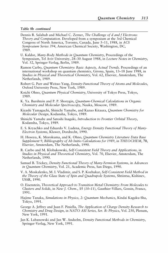
Table 8b continued

Dennis R. Salahub and Michael C. Zerner, The Challenge of d and f Electrons:Theory and Computation. Developed from a symposium at the 3rd ChemicalCongress of North America, Toronto, Canada, June 5–11, 1988, in ACSSymposium Series 394, American Chemical Society, Washington, DC,1989.

U. Kaldor, Many-Body Methods in Quantum Chemistry, Proceedings of theSymposium, Tel Aviv University, 28–30 August 1988, in Lecture Notes in Chemistry,Vol. 52, Springer-Verlag, Berlin, 1989.

Ramon Carbo, Quantum Chemistry: Basic Aspects, Actual Trends. Proceedings of aninternational workshop on quantum chemistry, Girona, Spain, 13–18 June 1988, inStudies in Physical and Theoretical Chemistry, Vol. 62, Elsevier, Amsterdam, TheNetherlands, 1989.

Robert G. Parr and Weitao Yang, Density-Functional Theory of Atoms and Molecules,Oxford University Press, New York, 1989.

Koichi Ohno, Quantum Physical Chemistry, University of Tokyo Press, Tokyo,1989.

K. Ya. Burshtein and P. P. Shorygin, Quantum-Chemical Calculations in OrganicChemistry and Molecular Spectroscopy, Nauka, Moscow, 1989.

Kizashi Yamaguchi, Shinichi Yamabe, and Kazuo Kitaura, Quantum Chemistry forMolecular Design, Kodansha, Tokyo, 1989.

Shinichi Yamabe and Satoshi Inagaki, Introduction to Frontier Orbital Theory,Kodansha, Tokyo, 1989.

E. S. Kryachko and Eduardo V. Ludena, Energy Density Functional Theory of Many-Electron Systems, Kluwer, Dordrecht, 1990.

H. Hosoya, K. Morokuma, and K. Ohno, Quantum Chemistry Literature Data BaseSupplement 9, Bibliography of Ab Initio Calculations for 1989, in THEOCHEM, 70,Elsevier, Amsterdam, The Netherlands, 1990.

R. Carbo and M. Klobukowski, Self-Consistent Field Theory and Applications, inStudies in Physical and Theoretical Chemistry, Vol. 70, Elsevier, Amsterdam, TheNetherlands, 1990.

Samuel B. Trickey, Density Functional Theory of Many-Fermion Systems, in Advancesin Quantum Chemistry, Vol. 21, Academic Press, San Diego, 1990.

V. A. Moskalenko, M. I. Vladimir, and S. P. Kozhukar, Self-Consistent Field Method inthe Theory of the Glass State of Spin and Quadrupole Systems, Shtiintsa, Kishinev,USSR, 1990.

O. Eisenstein, Theoretical Approach to Transition Metal Chemistry: From Molecules toClusters and Solids, in New J. Chem., 15 (10–11), Gauthier-Villars, Gossin, France,1991.

Hajime Tanaka, Simulations in Physics, 2: Quantum Mechanics, Kindai Kagaku-Sha,Tokyo, 1991.

George A. Jeffrey and Juan F. Piniella, The Application of Charge Density Research toChemistry and Drug Design, in NATO ASI Series, Ser. B: Physics, Vol. 250, Plenum,New York, 1991.

Jan K. Labanowski and Jan W. Andzelm, Density Functional Methods in Chemistry,Springer-Verlag, New York, 1991.

Quantum Chemistry 313

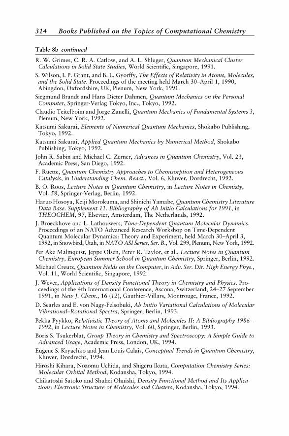
Table 8b continued

R. W. Grimes, C. R. A. Catlow, and A. L. Shluger, Quantum Mechanical ClusterCalculations in Solid State Studies, World Scientific, Singapore, 1991.

S. Wilson, I. P. Grant, and B. L. Gyorffy, The Effects of Relativity in Atoms, Molecules,and the Solid State. Proceedings of the meeting held March 30–April 1, 1990,Abingdon, Oxfordshire, UK, Plenum, New York, 1991.

Siegmund Brandt and Hans Dieter Dahmen, Quantum Mechanics on the PersonalComputer, Springer-Verlag Tokyo, Inc., Tokyo, 1992.

Claudio Teitelboim and Jorge Zanelli, Quantum Mechanics of Fundamental Systems 3,Plenum, New York, 1992.

Katsumi Sakurai, Elements of Numerical Quantum Mechanics, Shokabo Publishing,Tokyo, 1992.

Katsumi Sakurai, Applied Quantum Mechanics by Numerical Method, ShokaboPublishing, Tokyo, 1992.

John R. Sabin and Michael C. Zerner, Advances in Quantum Chemistry, Vol. 23,Academic Press, San Diego, 1992.

F. Ruette, Quantum Chemistry Approaches to Chemisorption and HeterogeneousCatalysis, in Understanding Chem. React., Vol. 6, Kluwer, Dordrecht, 1992.

B. O. Roos, Lecture Notes in Quantum Chemistry, in Lecture Notes in Chemisty,Vol. 58, Springer-Verlag, Berlin, 1992.

Haruo Hosoya, Keiji Morokuma, and Shinichi Yamabe, Quantum Chemistry LiteratureData Base. Supplement 11. Bibliography of Ab Initio Calculations for 1991, inTHEOCHEM, 97, Elsevier, Amsterdam, The Netherlands, 1992.

J. Broeckhove and L. Lathouwers, Time-Dependent Quantum Molecular Dynamics.Proceedings of an NATO Advanced Research Workshop on Time-DependentQuantum Molecular Dynamics: Theory and Experiment, held March 30–April 3,1992, in Snowbird, Utah, in NATO ASI Series, Ser. B., Vol. 299, Plenum, New York, 1992.

Per Ake Malmquist, Jeppe Olsen, Peter R. Taylor, et al., Lecture Notes in QuantumChemistry, European Summer School in Quantum Chemistry, Springer, Berlin, 1992.

Michael Creutz, Quantum Fields on the Computer, in Adv. Ser. Dir. High Energy Phys.,Vol. 11, World Scientific, Singapore, 1992.

J. Wever, Applications of Density Functional Theory in Chemistry and Physics. Pro-ceedings of the 4th International Conference, Ascona, Switzerland, 24–27 September1991, in New J. Chem., 16 (12), Gauthier-Villars, Montrouge, France, 1992.

D. Searles and E. von Nagy-Felsobuki, Ab Initio Variational Calculations of MolecularVibrational–Rotational Spectra, Springer, Berlin, 1993.

Pekka Pyykko, Relativistic Theory of Atoms and Molecules II: A Bibliography 1986–1992, in Lecture Notes in Chemistry, Vol. 60, Springer, Berlin, 1993.

Boris S. Tsukerblat, Group Theory in Chemistry and Spectroscopy: A Simple Guide toAdvanced Usage, Academic Press, London, UK, 1994.

Eugene S. Kryachko and Jean Louis Calais, Conceptual Trends in Quantum Chemistry,Kluwer, Dordrecht, 1994.

Hiroshi Kihara, Nozomu Uchida, and Shigeru Ikuta, Computation Chemistry Series:Molecular Orbital Method, Kodansha, Tokyo, 1994.

Chikatoshi Satoko and Shuhei Ohnishi, Density Functional Method and Its Applica-tions: Electronic Structure of Molecules and Clusters, Kodansha, Tokyo, 1994.

314 Books Published on the Topics of Computational Chemistry

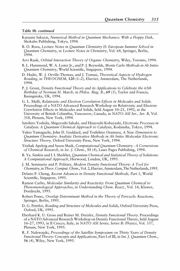
Table 8b continued

Katsumi Sakurai, Numerical Method in Quantum Mechanics: With a Floppy Disk,Shokabo Publishing, Tokyo, 1994.

B. O. Roos, Lecture Notes in Quantum Chemistry II: European Summer School inQuantum Chemistry, in Lecture Notes in Chemistry, Vol. 64, Springer, Berlin,1994.

Arvi Rauk, Orbital Interaction Theory of Organic Chemistry, Wiley, Toronto, 1994.

B. L. Hammond, W. A. Lester Jr., and P. J. Reynolds, Monte Carlo Methods in Ab InitioQuantum Chemistry, World Scientific, Singapore, 1994.

D. Hadzi, W. J. Orville-Thomas, and J. Tomasi, Theoretical Aspects of HydrogenBonding, in THEOCHEM, 120 (1–2), Elsevier, Amsterdam, The Netherlands,1994.

P. J. Grout, Density Functional Theory and its Applications to Celebrate the 65thBirthday of Norman H. March, in Philos. Mag. B., 69 (5), Taylor and Francis,Basingstoke, UK, 1994.

G. L. Malli, Relativistic and Electron Correlation Effects in Molecules and Solids.Proceedings of a NATO Advanced Research Workshop on Relativistic and ElectronCorrelation Effects in Molecules and Solids, held August 10–21, 1992, at theUniversity of British Columbia, Vancouver, Canada, in NATO ASI Ser., Ser. B, Vol.318, Plenum, New York, 1994.

Satohiro Yoshida, Shigeyoshi Sakaki, and Hisayoshi Kobayashi, Electronic Processes inCatalysis: A Quantum Chemical Approach to Catalysis, Kodansha, Tokyo, 1994.

Yukio Yamaguchi, John D. Goddard, and Yoshihiro Osamura, A New Dimension toQuantum Chemistry: Analytic Derivative Methods in Ab Initio Molecular ElectronicStructure Theory, Oxford University Press, New York, 1994.

Yitzhak Apeloig and Sason Shaik, Computational Quantum Chemistry - A Cornerstoneof Chemical Research, in Isr. J. Chem., 33 (4), Laser Pages Publishing, 1994.

B. Ya. Simkin and I. I. Sheikhet, Quantum Chemical and Statistical Theory of Solutions:A Computational Approach, Horwood, London, UK, 1995.

J. M. Seminario and P. Politzer, Modern Density Functional Theory: A Tool forChemistry, inTheor.Comput.Chem.,Vol.2,Elsevier,Amsterdam,TheNetherlands,1995.

Delano P. Chong, Recent Advances in Density Functional Methods, Part 1, WorldScientific, Singapore, 1995.

Ramon Carbo, Molecular Similarity and Reactivity: From Quantum Chemical toPhenomenological Approaches, in Understanding Chem. React., Vol. 14, Kluwer,Dordrecht, 1995.

Robert Ponec, Overlap Determinant Method in the Theory of Pericyclic Reactions,Springer, Berlin, 1995.

D. G. Pettifor, Bonding and Structure of Molecules and Solids, Oxford University Press,Oxford, UK, 1995.

Eberhard K. U. Gross and Reiner M. Dreizler, Density Functional Theory. Proceedingsof a NATO Advanced Research Workshop on Density Functional Theory, held August16–27, 1993, in Il Ciocco, Italy, in NATO ASI Series, Series B: Physics, Vol. 337,Plenum, New York, 1995.

R. F. Nalewajski, Proceedings of the Satellite Symposium on Thirty Years of DensityFunctional Theory: Concepts and Applications, Part I of III, in Int. J. Quantum Chem.,56 (4), Wiley, New York, 1995.

Quantum Chemistry 315

Table 8b continued

R. F. Nalewajski, Proceedings of the Satellite Symposium on Thirty Years of DensityFunctional Theory: Concepts and Applications, Part II of III, in Int. J. QuantumChem., 56 (5), Wiley, New York, 1995.

R. F. Nalewajski, Proceedings of the Satellite Symposium on Thirty Years of DensityFunctional Theory: Concepts and Applications, Part III of III, in Int. J. QuantumChem., 56 (6), Wiley, New York, 1995.

R. F. Nalewajski and J. Korchowiec, Advanced Series in Physical Chemistry, Vol. 8:Charge Sensitivity Approach to Electronic Structure and Chemical Sensitivity, WorldScientific, Singapore, 1995.

Anne-Marie Sapse and Paul von Rague Schleyer, Lithium Chemistry: A Theoretical andExperimental Overview, Wiley, New, York, 1995.

S. Yoshida, S. Sakaki, and H. Kobayashi, Electronic Processes in Catalysis: A QuantumChemical Approach to Catalysis, VCH, Weinheim, 1995.

David R. Yarkony, Modern Electronic Structure Theory: Part I, in Adv. Ser. Phys.Chem., Vol. 2, Pt. 1, World Scientific, Singapore, 1995.

David R. Yarkony, Modern Electronic Structure Theory: Part II, in Adv. Ser. Phys.Chem., Vol. 2, Pt. 2, World Scientific, Singapore, 1995.

Stephen R. Langhoff, Quantum Mechanical Electronic Structure Calculations withChemical Accuracy, in Understanding Chem. React., Vol. 13, Kluwer, Dordrecht, 1995.

Brian B Laird, Richard B. Ross, and Tom Ziegler, Chemical Applications of Density-Functional Theory, American Chemical Society, Washington, DC, 1996.

Constantinos A. Tsipis, Vladimir S. Popov, and Dudley R. Herschbach, New Methods inQuantum Theory. Proceedings of the NATO Advanced Research Workshop on NewMethods in Quantum Theory, held in Halkidiki, Greece, May 14–19, 1995, in NATOASI Ser., Ser. 3, Vol. 8, Kluwer, Dordrecht, 1996.

James R. Durig, A. J. Barnes, and W. J. Orville-Thomas, Spectroscopy and QuantumChemical Theory Applied to Problems in Molecular Structure. A collection ofinvited papers in honor of Professor James E. Boggs on the occasion of his 75thbirthday, in J. Mol. Struct., Vol. 376, Elsevier, Amsterdam, The Netherlands, 1996.

Thomas Klapoetke, Quantum Mechanical Methods in Main-Group Chemistry,Spektrum, Heidelberg, 1996.

John R. Sabin and Michael C. Zerner, Advances in Quantum Chemistry, Vol. 27,Academic Press, San Diego, 1996.

Karl Jug, Special Issue on Electronic Structure Methods for Truly Large Systems:Moving the Frontiers in Quantum Chemistry, Part II of II, in Int. J. Quantum Chem.,58 (3), Wiley, New York, 1996.

R. W. Robinett, Quantum Mechanics: Classical Results, Modern Systems, andVisualized Examples, Oxford University Press, Oxford, UK, 1996.

W. J. Hehre, Critical Assessment of Modern Electronic Structure Methods, Wavefunc-tion, Inc., Irvine, CA, 1996.

Dominique Bicout and Martin Field, Quantum Mechanical Simulation Methods forStudying Biological Systems, Les Houches Workshop, May 2–7, 1995, Springer,Berlin, 1996.

I. Prigogine and S. A. Rice, New Methods in Computational Quantum Mechanics, inAdv. Chem. Phys., Vol. 93, Wiley, New York, 1996.

A. A. Hasanein and M. W. Evans, Computational Methods in Quantum Chemistry,Vol. 2: Quantum Chemistry, World Scientific, Singapore, 1996.

316 Books Published on the Topics of Computational Chemistry

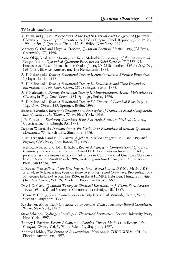
Table 8b continued

R. Polak and J. Fiser, Proceedings of the Eighth International Congress of QuantumChemistry. Proceedings of a conference held in Prague, Czech Republic, June 19–23,1994, in Int. J. Quantum Chem., 57 (5), Wiley, New York, 1996.

Margery G. Ord and Lloyd A. Stocken, Quantum Leaps in Biochemistry, JAI Press,Greenwich, CT, 1996.

Ayao Okiji, Yoshitada Murata, and Kenji Makoshi, Proceedings of the InternationalSymposium on Dynamical Quantum Processes on Solid Surfaces (DQPSS ’95).Proceedings of a conference held in Osaka, Japan, 20–22 September 1995, in Surf. Sci.,363 (1–3), Elsevier, Amsterdam, The Netherlands, 1996.

R. F. Nalewajski, Density Functional Theory I: Functionals and Effective Potentials,Springer, Berlin, 1996.

R. F. Nalewajski, Density Functional Theory II: Relativistic and Time DependentExtensions, in Top. Curr. Chem., 181, Springer, Berlin, 1996.

R. F. Nalewajski, Density Functional Theory III: Interpretation, Atoms, Molecules andClusters, in Top. Curr. Chem., 182, Springer, Berlin, 1996.

R. F. Nalewajski, Density Functional Theory IV: Theory of Chemical Reactivity, inTop. Curr. Chem., 183, Springer, Berlin, 1996.

Isaac B. Bersuker, Electronic Structure and Properties of Transition Metal Compounds:Introduction to the Theory, Wiley, New York, 1996.

J. B. Foresman, Exploring Chemistry With Electronic Structure Methods, 2nd ed.,Gaussian, Inc., Pittsburgh, PA, 1996.

Stephen Wilson, An Introduction to the Methods of Relativistic Molecular QuantumMechanics, World Scientific, Singapore, 1996.

F. M. Fernandez and E. A. Castro, Algebraic Methods in Quantum Chemistry andPhysics, CRC Press, Boca Raton, FL, 1996.

Jacek Karwowski and John R. Sabin, Recent Advances in Computational QuantumChemistry. Papers written to honor Geerd H. F. Diercksen on his 60th birthdaypresented at the symposium Recent Advances in Computational Quantum Chemistryheld in Munich, 29–30 March 1996, in Adv. Quantum Chem., Vol. 28, AcademicPress, San Diego, 1997.

L. Kover, Proceedings of the First International Workshop on DV-X.a Method DV-X.a ’96, with Special Emphasis on Inner-Shell Physics and Chemistry. Proceedings of aconference held 2–3 September 1996, in the ATOMKI, Debrecen, Hungary, in Adv.Quantum Chem., Vol. 29, Academic Press, San Diego, 1997.

David C. Clary, Quantum Theory of Chemical Reactions, in J. Chem. Soc., FaradayTrans., 93 (5), Royal Society of Chemistry, Cambridge, UK, 1997.

Delano P. Chong, Recent Advances in Density Functional Methods, Part 2, WorldScientific, Singapore, 1997.

S. Scheiner, Molecular Interactions. From van der Waals to Strongly Bound Complexes,Wiley, New York, 1997.

Steve Scheiner, Hydrogen Bonding: A Theoretical Perspective, Oxford University Press,New York, 1997.

Rodney J. Bartlett, Recent Advances in Coupled-Cluster Methods, in Recent Adv.Comput. Chem., Vol. 3, World Scientific, Singapore, 1997.

Andrew Holder, The Future of Semiempirical Methods, in THEOCHEM, 401 (3),Elsevier, Amsterdam, 1997.

Quantum Chemistry 317

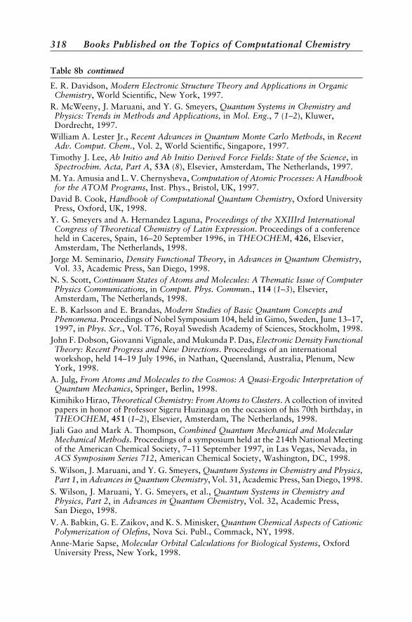
Table 8b continued

E. R. Davidson, Modern Electronic Structure Theory and Applications in OrganicChemistry, World Scientific, New York, 1997.

R. McWeeny, J. Maruani, and Y. G. Smeyers, Quantum Systems in Chemistry andPhysics: Trends in Methods and Applications, in Mol. Eng., 7 (1–2), Kluwer,Dordrecht, 1997.

William A. Lester Jr., Recent Advances in Quantum Monte Carlo Methods, in RecentAdv. Comput. Chem., Vol. 2, World Scientific, Singapore, 1997.

Timothy J. Lee, Ab Initio and Ab Initio Derived Force Fields: State of the Science, inSpectrochim. Acta, Part A, 53A (8), Elsevier, Amsterdam, The Netherlands, 1997.

M. Ya. Amusia and L. V. Chernysheva, Computation of Atomic Processes: A Handbookfor the ATOM Programs, Inst. Phys., Bristol, UK, 1997.

David B. Cook, Handbook of Computational Quantum Chemistry, Oxford UniversityPress, Oxford, UK, 1998.

Y. G. Smeyers and A. Hernandez Laguna, Proceedings of the XXIIIrd InternationalCongress of Theoretical Chemistry of Latin Expression. Proceedings of a conferenceheld in Caceres, Spain, 16–20 September 1996, in THEOCHEM, 426, Elsevier,Amsterdam, The Netherlands, 1998.

Jorge M. Seminario, Density Functional Theory, in Advances in Quantum Chemistry,Vol. 33, Academic Press, San Diego, 1998.

N. S. Scott, Continuum States of Atoms and Molecules: A Thematic Issue of ComputerPhysics Communications, in Comput. Phys. Commun., 114 (1–3), Elsevier,Amsterdam, The Netherlands, 1998.

E. B. Karlsson and E. Brandas, Modern Studies of Basic Quantum Concepts andPhenomena. Proceedings of Nobel Symposium 104, held in Gimo, Sweden, June 13–17,1997, in Phys. Scr., Vol. T76, Royal Swedish Academy of Sciences, Stockholm, 1998.

John F. Dobson, Giovanni Vignale, and Mukunda P. Das, Electronic Density FunctionalTheory: Recent Progress and New Directions. Proceedings of an internationalworkshop, held 14–19 July 1996, in Nathan, Queensland, Australia, Plenum, NewYork, 1998.

A. Julg, From Atoms and Molecules to the Cosmos: A Quasi-Ergodic Interpretation ofQuantum Mechanics, Springer, Berlin, 1998.

Kimihiko Hirao, Theoretical Chemistry: From Atoms to Clusters. A collection of invitedpapers in honor of Professor Sigeru Huzinaga on the occasion of his 70th birthday, inTHEOCHEM, 451 (1–2), Elsevier, Amsterdam, The Netherlands, 1998.

Jiali Gao and Mark A. Thompson, Combined Quantum Mechanical and MolecularMechanical Methods. Proceedings of a symposium held at the 214th National Meetingof the American Chemical Society, 7–11 September 1997, in Las Vegas, Nevada, inACS Symposium Series 712, American Chemical Society, Washington, DC, 1998.

S. Wilson, J. Maruani, and Y. G. Smeyers, Quantum Systems in Chemistry and Physics,Part 1, in Advances in Quantum Chemistry, Vol. 31, Academic Press, San Diego, 1998.

S. Wilson, J. Maruani, Y. G. Smeyers, et al., Quantum Systems in Chemistry andPhysics, Part 2, in Advances in Quantum Chemistry, Vol. 32, Academic Press,San Diego, 1998.

V. A. Babkin, G. E. Zaikov, and K. S. Minisker, Quantum Chemical Aspects of CationicPolymerization of Olefins, Nova Sci. Publ., Commack, NY, 1998.

Anne-Marie Sapse, Molecular Orbital Calculations for Biological Systems, OxfordUniversity Press, New York, 1998.

318 Books Published on the Topics of Computational Chemistry

Table 8b continued

Fernando Bernardi and Fernando M. S. Silva Fernandes, Computational Chemistry1997. A Selection of Papers from the Second European Conference, held 2–6September 1997, Lisbon, Portugal, in THEOCHEM, 463 (1–2), Elsevier, Amsterdam,The Netherlands, 1999.

John R. Sabin, Michael C. Zerner, and Erkki Brandas, Advances in QuantumChemistry, Vol. 34, Academic Press, San Diego, 1999.

Gernot Frenking, Progress in Density Functional Theory, in J. Comput. Chem., 20 (1),Wiley, New York, 1999.

Arthur Greenberg, Curt M. Breneman, and Joel F. Liebman, The Amide Linkage:Structural Significance in Chemistry, Biochemistry, and Materials Science, Wiley,New York, 1999.

Martin Kaupp and Vladimir G. Malkin, Quantum Chemical Calculations of NMR andEPR Parameters. Proceedings of a symposium held 14-18 September 1998 at theSmolenice Castle near Bratislava, Slovak Republic, in J. Comput. Chem., 20 (12),Wiley, New York, 1999.

Yves G. Smeyers and Sylvio Canuto, Proceedings of the Ninth Brazilian Symposium ofTheoretical Chemistry, held 16-19 November 1997, Caxambu, Brazil, in THEO-CHEM, 464 (1–3), Elsevier, Amsterdam, Neth., 1999.

Per Jensen and Philip R. Bunker, Computational Molecular Spectroscopy, Wiley,New York, 2000.

Arvi Rauk, Orbital Interaction Theory of Organic Chemistry, 2nd ed., Wiley,New York, 2000.

Friedel Hossfield, Reinhard Ahlrichs, Peter Taylor, and Donald G. Truhlar, ParallelComputing in Chemical Physics: A Thematic Issue of Computer Physics Commu-nications, in Comput. Phys. Commun., 128 (1–2), Elsevier, Amsterdam, 2000.

Walter A. Harrison, Applied Quantum Mechanics, World Scientific, Singapore, 2000.

Brian N. Figgis and Michael A. Hitchman, Ligand Field Theory and Its Applications.Wiley-VCH, New York, 2000.

W. Koch, A Chemist’s Guide to Density Functional Theory, Wiley-VCH, Weinheim,2000.

Crystals, Polymers, and Materials

Table 8c Quantum Chemistry Books on Crystals, Polymers, and Materials

Berni J. Alder, Sidney Fernbach, and Manual Rotenberg, Energy Bands of Solids,Academic Press, New York, 1968.

Richard L. Longini, Introductory Quantum Mechanics for the Solid State, Interscience,New York, 1970.

Philip L. Taylor, A Quantum Approach to the Solid State, Prentice Hall, EnglewoodCliffs, NJ, 1970.

P. M. Marcus, F. Janak, and A. R. Williams, Computational Methods in Band Theory,Proceedings of the Conference held in Yorktown Heights, New York, May 14–15,1970, Plenum, New York, 1971.

C. George, I. Prigogine, and L. Rosenfeld, The Macroscopic Level of QuantumMechanics, Munksgaard, Copenhagen, 1972.

Quantum Chemistry 319

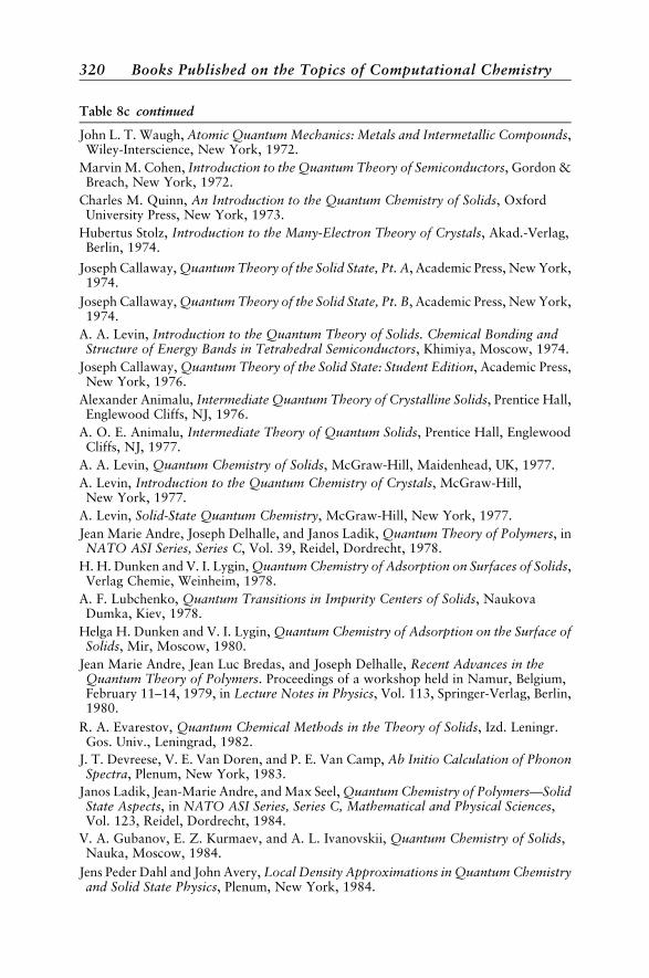
Table 8c continued

John L. T. Waugh, Atomic Quantum Mechanics: Metals and Intermetallic Compounds,Wiley-Interscience, New York, 1972.

Marvin M. Cohen, Introduction to the Quantum Theory of Semiconductors, Gordon &Breach, New York, 1972.

Charles M. Quinn, An Introduction to the Quantum Chemistry of Solids, OxfordUniversity Press, New York, 1973.

Hubertus Stolz, Introduction to the Many-Electron Theory of Crystals, Akad.-Verlag,Berlin, 1974.

Joseph Callaway, Quantum Theory of the Solid State, Pt. A, Academic Press, New York,1974.

Joseph Callaway, Quantum Theory of the Solid State, Pt. B, Academic Press, New York,1974.

A. A. Levin, Introduction to the Quantum Theory of Solids. Chemical Bonding andStructure of Energy Bands in Tetrahedral Semiconductors, Khimiya, Moscow, 1974.

Joseph Callaway, Quantum Theory of the Solid State: Student Edition, Academic Press,New York, 1976.

Alexander Animalu, Intermediate Quantum Theory of Crystalline Solids, Prentice Hall,Englewood Cliffs, NJ, 1976.

A. O. E. Animalu, Intermediate Theory of Quantum Solids, Prentice Hall, EnglewoodCliffs, NJ, 1977.

A. A. Levin, Quantum Chemistry of Solids, McGraw-Hill, Maidenhead, UK, 1977.

A. Levin, Introduction to the Quantum Chemistry of Crystals, McGraw-Hill,New York, 1977.

A. Levin, Solid-State Quantum Chemistry, McGraw-Hill, New York, 1977.

Jean Marie Andre, Joseph Delhalle, and Janos Ladik, Quantum Theory of Polymers, inNATO ASI Series, Series C, Vol. 39, Reidel, Dordrecht, 1978.

H. H. Dunken and V. I. Lygin, Quantum Chemistry of Adsorption on Surfaces of Solids,Verlag Chemie, Weinheim, 1978.

A. F. Lubchenko, Quantum Transitions in Impurity Centers of Solids, NaukovaDumka, Kiev, 1978.

Helga H. Dunken and V. I. Lygin, Quantum Chemistry of Adsorption on the Surface ofSolids, Mir, Moscow, 1980.

Jean Marie Andre, Jean Luc Bredas, and Joseph Delhalle, Recent Advances in theQuantum Theory of Polymers. Proceedings of a workshop held in Namur, Belgium,February 11–14, 1979, in Lecture Notes in Physics, Vol. 113, Springer-Verlag, Berlin,1980.

R. A. Evarestov, Quantum Chemical Methods in the Theory of Solids, Izd. Leningr.Gos. Univ., Leningrad, 1982.

J. T. Devreese, V. E. Van Doren, and P. E. Van Camp, Ab Initio Calculation of PhononSpectra, Plenum, New York, 1983.

Janos Ladik, Jean-Marie Andre, and Max Seel, Quantum Chemistry of Polymers—SolidState Aspects, in NATO ASI Series, Series C, Mathematical and Physical Sciences,Vol. 123, Reidel, Dordrecht, 1984.

V. A. Gubanov, E. Z. Kurmaev, and A. L. Ivanovskii, Quantum Chemistry of Solids,Nauka, Moscow, 1984.

Jens Peder Dahl and John Avery, Local Density Approximations in Quantum Chemistryand Solid State Physics, Plenum, New York, 1984.

320 Books Published on the Topics of Computational Chemistry

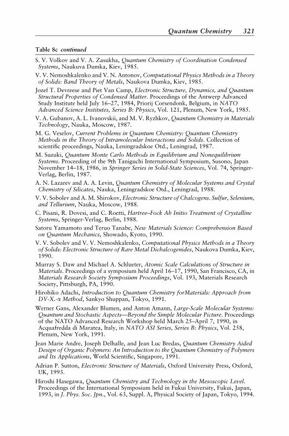
Table 8c continued

S. V. Volkov and V. A. Zasukha, Quantum Chemistry of Coordination CondensedSystems, Naukuva Dumka, Kiev, 1985.

V. V. Nemoshkalenko and V. N. Antonov, Computational Physics Methods in a Theoryof Solids: Band Theory of Metals, Naukova Dumka, Kiev, 1985.

Jozef T. Devreese and Piet Van Camp, Electronic Structure, Dynamics, and QuantumStructural Properties of Condensed Matter. Proceedings of the Antwerp AdvancedStudy Institute held July 16–27, 1984, Priorij Corsendonk, Belgium, in NATOAdvanced Science Institutes, Series B: Physics, Vol. 121, Plenum, New York, 1985.

V. A. Gubanov, A. L. Ivanovskii, and M. V. Ryzhkov, Quantum Chemistry in MaterialsTechnology, Nauka, Moscow, 1987.

M. G. Veselov, Current Problems in Quantum Chemistry: Quantum ChemistryMethods in the Theory of Intramolecular Interactions and Solids. Collection ofscientific proceedings, Nauka, Leningradskoe Otd., Leningrad, 1987.

M. Suzuki, Quantum Monte Carlo Methods in Equilibrium and NonequilibriumSystems. Proceeding of the 9th Taniguchi International Symposium, Susono, JapanNovember 14–18, 1986, in Springer Series in Solid-State Sciences, Vol. 74, Springer-Verlag, Berlin, 1987.

A. N. Lazarev and A. A. Levin, Quantum Chemistry of Molecular Systems and CrystalChemistry of Silicates, Nauka, Leningradskoe Otd., Leningrad, 1988.

V. V. Sobolev and A. M. Shirokov, Electronic Structure of Chalcogens. Sulfur, Selenium,and Tellurium, Nauka, Moscow, 1988.

C. Pisani, R. Dovesi, and C. Roetti, Hartree–Fock Ab Initio Treatment of CrystallineSystems, Springer-Verlag, Berlin, 1988.

Satoru Yamamoto and Teruo Tanabe, New Materials Science: Comprehension Basedon Quantum Mechanics, Showado, Kyoto, 1990.

V. V. Sobolev and V. V. Nemoshkalenko, Computational Physics Methods in a Theoryof Solids: Electronic Structure of Rare Metal Dichalcogenides, Naukova Dumka, Kiev,1990.

Murray S. Daw and Michael A. Schlueter, Atomic Scale Calculations of Structure inMaterials. Proceedings of a symposium held April 16–17, 1990, San Francisco, CA, inMaterials Research Society Symposium Proceedings, Vol. 193, Materials ResearchSociety, Pittsburgh, PA, 1990.

Hirohiko Adachi, Introduction to Quantum Chemistry forMaterials: Approach fromDV-X.-a Method, Sankyo Shuppan, Tokyo, 1991.

Werner Gans, Alexander Blumen, and Anton Amann, Large-Scale Molecular Systems:Quantum and Stochastic Aspects—Beyond the Simple Molecular Picture. Proceedingsof the NATO Advanced Research Workshop held March 25–April 7, 1990, inAcquafredda di Maratea, Italy, in NATO ASI Series, Series B: Physics, Vol. 258,Plenum, New York, 1991.

Jean Marie Andre, Joseph Delhalle, and Jean Luc Bredas, Quantum Chemistry AidedDesign of Organic Polymers: An Introduction to the Quantum Chemistry of Polymersand Its Applications, World Scientific, Singapore, 1991.

Adrian P. Sutton, Electronic Structure of Materials, Oxford University Press, Oxford,UK, 1993.

Hiroshi Hasegawa, Quantum Chemistry and Technology in the Mesoscopic Level.Proceedings of the International Symposium held in Fukui University, Fukui, Japan,1993, in J. Phys. Soc. Jpn., Vol. 63, Suppl. A, Physical Society of Japan, Tokyo, 1994.

Quantum Chemistry 321

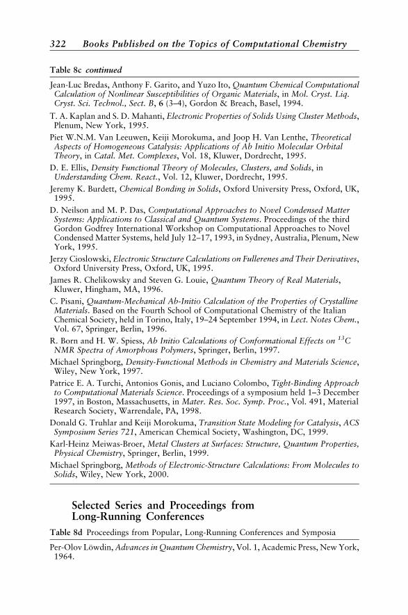
Table 8c continued

Jean-Luc Bredas, Anthony F. Garito, and Yuzo Ito, Quantum Chemical ComputationalCalculation of Nonlinear Susceptibilities of Organic Materials, in Mol. Cryst. Liq.Cryst. Sci. Technol., Sect. B, 6 (3–4), Gordon & Breach, Basel, 1994.

T. A. Kaplan and S. D. Mahanti, Electronic Properties of Solids Using Cluster Methods,Plenum, New York, 1995.

Piet W.N.M. Van Leeuwen, Keiji Morokuma, and Joop H. Van Lenthe, TheoreticalAspects of Homogeneous Catalysis: Applications of Ab Initio Molecular OrbitalTheory, in Catal. Met. Complexes, Vol. 18, Kluwer, Dordrecht, 1995.

D. E. Ellis, Density Functional Theory of Molecules, Clusters, and Solids, inUnderstanding Chem. React., Vol. 12, Kluwer, Dordrecht, 1995.

Jeremy K. Burdett, Chemical Bonding in Solids, Oxford University Press, Oxford, UK,1995.

D. Neilson and M. P. Das, Computational Approaches to Novel Condensed MatterSystems: Applications to Classical and Quantum Systems. Proceedings of the thirdGordon Godfrey International Workshop on Computational Approaches to NovelCondensed Matter Systems, held July 12–17, 1993, in Sydney, Australia, Plenum, NewYork, 1995.

Jerzy Cioslowski, Electronic Structure Calculations on Fullerenes and Their Derivatives,Oxford University Press, Oxford, UK, 1995.

James R. Chelikowsky and Steven G. Louie, Quantum Theory of Real Materials,Kluwer, Hingham, MA, 1996.

C. Pisani, Quantum-Mechanical Ab-Initio Calculation of the Properties of CrystallineMaterials. Based on the Fourth School of Computational Chemistry of the ItalianChemical Society, held in Torino, Italy, 19–24 September 1994, in Lect. Notes Chem.,Vol. 67, Springer, Berlin, 1996.

R. Born and H. W. Spiess, Ab Initio Calculations of Conformational Effects on 13CNMR Spectra of Amorphous Polymers, Springer, Berlin, 1997.

Michael Springborg, Density-Functional Methods in Chemistry and Materials Science,Wiley, New York, 1997.

Patrice E. A. Turchi, Antonios Gonis, and Luciano Colombo, Tight-Binding Approachto Computational Materials Science. Proceedings of a symposium held 1–3 December1997, in Boston, Massachusetts, in Mater. Res. Soc. Symp. Proc., Vol. 491, MaterialResearch Society, Warrendale, PA, 1998.

Donald G. Truhlar and Keiji Morokuma, Transition State Modeling for Catalysis, ACSSymposium Series 721, American Chemical Society, Washington, DC, 1999.

Karl-Heinz Meiwas-Broer, Metal Clusters at Surfaces: Structure, Quantum Properties,Physical Chemistry, Springer, Berlin, 1999.

Michael Springborg, Methods of Electronic-Structure Calculations: From Molecules toSolids, Wiley, New York, 2000.

Selected Series and Proceedings fromLong-Running Conferences

Table 8d Proceedings from Popular, Long-Running Conferences and Symposia

Per-Olov Lowdin, Advances in Quantum Chemistry, Vol. 1, Academic Press, New York,1964.

322 Books Published on the Topics of Computational Chemistry

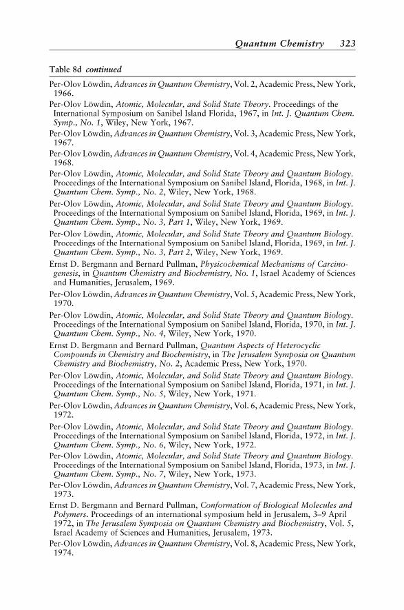
Table 8d continued

Per-Olov Lowdin, Advances in Quantum Chemistry, Vol. 2, Academic Press, New York,1966.

Per-Olov Lowdin, Atomic, Molecular, and Solid State Theory. Proceedings of theInternational Symposium on Sanibel Island Florida, 1967, in Int. J. Quantum Chem.Symp., No. 1, Wiley, New York, 1967.

Per-Olov Lowdin, Advances in Quantum Chemistry, Vol. 3, Academic Press, New York,1967.

Per-Olov Lowdin, Advances in Quantum Chemistry, Vol. 4, Academic Press, New York,1968.

Per-Olov Lowdin, Atomic, Molecular, and Solid State Theory and Quantum Biology.Proceedings of the International Symposium on Sanibel Island, Florida, 1968, in Int. J.Quantum Chem. Symp., No. 2, Wiley, New York, 1968.

Per-Olov Lowdin, Atomic, Molecular, and Solid State Theory and Quantum Biology.Proceedings of the International Symposium on Sanibel Island, Florida, 1969, in Int. J.Quantum Chem. Symp., No. 3, Part 1, Wiley, New York, 1969.

Per-Olov Lowdin, Atomic, Molecular, and Solid State Theory and Quantum Biology.Proceedings of the International Symposium on Sanibel Island, Florida, 1969, in Int. J.Quantum Chem. Symp., No. 3, Part 2, Wiley, New York, 1969.

Ernst D. Bergmann and Bernard Pullman, Physicochemical Mechanisms of Carcino-genesis, in Quantum Chemistry and Biochemistry, No. 1, Israel Academy of Sciencesand Humanities, Jerusalem, 1969.

Per-Olov Lowdin, Advances in Quantum Chemistry, Vol. 5, Academic Press, New York,1970.

Per-Olov Lowdin, Atomic, Molecular, and Solid State Theory and Quantum Biology.Proceedings of the International Symposium on Sanibel Island, Florida, 1970, in Int. J.Quantum Chem. Symp., No. 4, Wiley, New York, 1970.

Ernst D. Bergmann and Bernard Pullman, Quantum Aspects of HeterocyclicCompounds in Chemistry and Biochemistry, in The Jerusalem Symposia on QuantumChemistry and Biochemistry, No. 2, Academic Press, New York, 1970.

Per-Olov Lowdin, Atomic, Molecular, and Solid State Theory and Quantum Biology.Proceedings of the International Symposium on Sanibel Island, Florida, 1971, in Int. J.Quantum Chem. Symp., No. 5, Wiley, New York, 1971.

Per-Olov Lowdin, Advances in Quantum Chemistry, Vol. 6, Academic Press, New York,1972.

Per-Olov Lowdin, Atomic, Molecular, and Solid State Theory and Quantum Biology.Proceedings of the International Symposium on Sanibel Island, Florida, 1972, in Int. J.Quantum Chem. Symp., No. 6, Wiley, New York, 1972.

Per-Olov Lowdin, Atomic, Molecular, and Solid State Theory and Quantum Biology.Proceedings of the International Symposium on Sanibel Island, Florida, 1973, in Int. J.Quantum Chem. Symp., No. 7, Wiley, New York, 1973.

Per-Olov Lowdin, Advances in Quantum Chemistry, Vol. 7, Academic Press, New York,1973.

Ernst D. Bergmann and Bernard Pullman, Conformation of Biological Molecules andPolymers. Proceedings of an international symposium held in Jerusalem, 3–9 April1972, in The Jerusalem Symposia on Quantum Chemistry and Biochemistry, Vol. 5,Israel Academy of Sciences and Humanities, Jerusalem, 1973.

Per-Olov Lowdin, Advances in Quantum Chemistry, Vol. 8, Academic Press, New York,1974.

Quantum Chemistry 323

Table 8d continued

Ernst D. Bergmann and Bernard Pullman, Chemical and Biochemical Reactivity,Proceedings of an international symposium held in Jerusalem, 9–13 April 1973, in TheJerusalem Symposia on Quantum Chemistry and Biochemistry, Vol. 6, Israel Academyof Sciences and Humanities, Jerusalem, 1974.

Ernst D. Bergmann and Bernard Pullman, Molecular and Quantum Pharmacology.Proceedings of the Seventh Jerusalem Symposium on Quantum Chemistry andBiochemistry held in Jerusalem, March 31–April 4, 1974 in The Jerusalem Symposiaon Quantum Chemistry and Biochemistry, Vol. 7, Reidel, Boston,1974.

Per-Olov Lowdin, Atomic, Molecular, and Solid State Theory and Quantum Statistics.Proceedings of the International Symposium on Sanibel Island, Florida, 1974, in Int. J.Quantum Chem. Symp., No. 8, Wiley, New York, 1974.

Per-Olov Lowdin, Quantum Biology and Quantum Pharmacology. Proceedings of theInternational Symposium on Sanibel Island, Florida, January 17–19, 1974, in Int. J.Quantum Chem., Quantum Biol. Symp., No. 1, Wiley, New York, 1974.

Per-Olov Lowdin, Quantum Biology and Quantum Pharmacology. Proceedings of theInternational Symposium on Sanibel Island, Florida, January 16–18, 1975, in Int. J.Quantum Chem., Quantum Biol. Symp., No. 2, Wiley, New York, 1975.

Per-Olov Lowdin, Advances in Quantum Chemistry, Vol. 9, Academic Press, New York,1975.

Per-Olov Lowdin, Atomic, Molecular, and Solid State Theory and Quantum Statistics.Proceedings of the International Symposium on Sanibel Island, Florida, 1975, in Int. J.Quantum Chem. Symp., No. 9, Wiley, New York, 1975.

Bernard Pullman, Environmental Effects on Molecular Structure and Properties,Proceedings of an international symposium held in Jerusalem, 7–11 April, 1975, in TheJerusalem Symposia on Quantum Chemistry and Biochemistry, Vol. 8, Reidel,Dordrecht, 1976.

Per-Olov Lowdin, Atomic, Molecular, and Solid State Theory and Quantum Statistics.Proceedings of the International Symposium on Sanibel Island, Florida, 1976, in Int. J.Quantum Chem. Symp., No. 10, Wiley, New York, 1976.

Per-Olov Lowdin and Yngve Ohrn, Atomic, Molecular, and Solid State Theory,Collision Phenomena, and Computational Methods. Proceedings of the InternationalSymposium on Sanibel Island, Florida, 1977, in Int. J. Quantum Chem. Symp., No. 11,Wiley, New York, 1977.

Per-Olov Lowdin and John R. Sabin, Quantum Biology and Quantum Pharmacology.Proceedings of the International Symposium on Sanibel Island, Florida, January 12–14,1976, in Int. J. Quantum Chem., Quantum Biol. Symp., No. 3, Wiley, New York,1976.

Per-Olov Lowdin, Advances in Quantum Chemistry, Vol. 10, Academic Press,New York, 1977.

Per-Olov Lowdin and John R. Sabin, Quantum Biology and Quantum Pharmacology.Proceedings of the International Symposium on Sanibel Island, Florida, January 9–12,1977, in Int. J. Quantum Chem., Quantum Biol. Symp., No. 4, Wiley, New York,1977.

Bernard Pullman and Natan Goldblum, Metal–Ligand Interactions in OrganicChemistry and Biochemistry, in The Jerusalem Symposia on Quantum Chemistry andBiochemistry, Vol. 9, Pt. 1, Reidel, Dordrecht, 1977.

324 Books Published on the Topics of Computational Chemistry

Table 8d continued

Bernard Pullman and Natan Goldblum, Excited States in Organic Chemistry andBiochemistry, in The Jerusalem Symposia on Quantum Chemistry and Biochemistry,Vol. 10, Reidel, Dordrecht, 1977.

Per-Olov Lowdin and Yngve Ohrn, Atomic, Molecular, and Solid-State Theory,Collision Phenomena, and Computational Methods. Proceedings of the InternationalSymposium held at Flagler Beach, Florida, in 1978, in Int. J. Quantum Chem.,Quantum Chem. Symp., No. 12, Wiley, New York, 1978.

Per-Olov Lowdin, Jean Louis Calais, and Osvaldo Goscinski, Quantum Chemistry—A Scientific Melting Pot. Proceedings of a symposium in Uppsala, Sweden, 1977, inInt. J. Quantum Chem., No. 12 (Suppl.), Wiley, New York, 1978.

Per-Olov Lowdin, Advances in Quantum Chemistry, Vol. 11, Academic Press,New York, 1978.

Per-Olov Lowdin and John R. Sabin, Quantum Biology and Quantum Pharmacology.Proceedings of the International Symposium held at Flagler Beach, Florida, March 3–11, 1978, in Int. J. Quantum Chem., Quantum Biol. Symp., No. 5, Wiley, New York,1978.

Bernard Pullman, Nuclear Magnetic Resonance Spectroscopy in Molecular Biology, inThe Jerusalem Symposia on Quantum Chemistry and Biochemistry, Vol. 11, Reidel,Dordrecht, 1978.

Per-Olov Lowdin and John R. Sabin, Quantum Biology and Quantum Pharmacology.Proceedings of the International Symposium on Sanibel Island, Florida, March 4–10,1979, in Int. J. Quantum Chem., Quantum Biol. Symp., No. 6, Wiley, New York, 1979.

Bernard Pullman, Catalysis in Chemistry and Biochemistry, Theory and Experiment, inThe Jerusalem Symposia on Quantum Chemistry and Biochemistry, Vol. 12, Reidel,Dordrecht, 1979.

Per-Olov Lowdin and Yngve Ohrn, Atomic, Molecular, and Solid-State Theory,Collision Phenomena, Quantum Statistics, and Computational Method. Proceedingsof the International Symposium held at Flagler Beach, Florida, March 11–17, 1979, inInt. J. Quantum Chem., Quantum Chem. Symp., No. 13, Wiley, New York, 1979.

Per-Olov Lowdin and Yngve Ohrn, Atomic, Molecular, and Solid-State Theory,Collision Phenomena, Quantum Statistics, and Computational Method. Proceedingsof the International Symposium held at Flagler Beach, Florida, March 10–20, 1980, inInt. J. Quantum Chem., Quantum Chem. Symp., No. 14, Wiley, New York, 1980.

Per-Olov Lowdin and John R. Sabin, Quantum Biology and Quantum Pharmacology.Proceedings of the International Symposium held at Palm Coast, Florida, March 5–8,1980, in Int. J. Quantum Chem., Quantum Biol. Symp., Vol. 7, Wiley, New York, 1980.

Per-Olov Lowdin, Advances in Quantum Chemistry, Vol. 12, Academic Press,New York, 1980.

Bernard Pullman, Paul O. P. Ts’o, and Harry Gelboin, Carcinogenesis: FundamentalMechanisms and Environmental Effects, in The Jerusalem Symposia on QuantumChemistry and Biochemistry, Vol. 13, Riedel, Dordrecht, 1980.

Per-Olov Lowdin and Yngve Ohrn, Atomic, Molecular, and Solid-State Theory,Collision Phenomena, and Computational Quantum Chemistry. Proceedings of theInternational Symposium held at Flagler Beach, Florida, March 8–14, 1981, in Int. J.Quantum Chem., Quantum Chem. Symp., Vol. 15, Wiley, New York, 1981.

Bernard Pullman, Intermolecular Forces, in The Jerusalem Symposia on QuantumChemistry and Biochemistry, Vol. 14, Reidel, Dordrecht, 1981.

Quantum Chemistry 325

Table 8d continued

Per-Olov Lowdin, Advances in Quantum Chemistry, Vol. 13, Academic Press,New York, 1981.

Per-Olov Lowdin, Advances in Quantum Chemistry, Vol. 14, Academic Press,New York, 1981.

Per-Olov Lowdin and John R. Sabin, Quantum Biology and Quantum Pharmacology.Proceedings of the International Symposium held at Palm Coast, Florida, March 5–7,1981, in Int. J. Quantum Chem., Quantum Biol. Symp., Vol. 8, Wiley, New York,1981.

Per-Olov Lowdin, Advances in Quantum Chemistry, Vol. 15, Academic Press,New York, 1982.

Per-Olov Lowdin, Advances in Quantum Chemistry, Vol. 16, Academic Press,New York, 1982.

Per-Olov Lowdin and John R. Sabin, Quantum Biology and Quantum Pharmacology.Proceedings of the International Symposium held at Palm Coast, Florida, March 4–6,1982, in Int. J. Quantum Chem., Quantum Biol. Symp., Vol. 9, Wiley, New York,1982.

Bernard Pullman and Joshua Jortner, Intermolecular Dynamics, in The JerusalemSymposia on Quantum Chemistry and Biochemistry, Vol. 15, Reidel, Dordrecht,1982.

Per-Olov Lowdin and Yngve Ohrn, Quantum Chemistry, Theory of Condensed Matter,and Propagator Methods in the Quantum Theory of Matter. Proceedings of theInternational Symposium held at Flagler Beach, Florida, March 1–3 and 7–13, 1982, inInt. J. Quantum Chem., Quantum Chem. Symp., No. 16, Wiley, New York, 1982.

Per-Olov Lowdin and Michael C. Zerner, Quantum Biology and QuantumPharmacology. Proceedings of the International Symposium held at Palm Coast,Florida, March 14–16, 1983, in Int. J. Quantum Chem., Quantum Biol. Symp., No. 10,Wiley, New York, 1983.

Per-Olov Lowdin and Yngve Ohrn. Guest Editor: David Micha, Atomic, Molecular andSolid-State Theory, Collision Phenomena, and Computational Quantum Chemistry.Proceedings of the International Symposium held at Flagler Beach, Florida, March3–12, 1983, in Int. J. Quantum Chem., Quantum Chem. Symp., No. 17, Wiley, NewYork, 1983.

Per-Olov Lowdin and Bernard Pullman, New Horizons of Quantum Chemistry.Proceedings of the 4th International Congress held at Uppsala, Sweden, June 14–19,1982, Reidel, Dordrecht, 1983.

Bernard Pullman and Joshua Jortner, Nucleic Acids: The Vectors of Life, in TheJerusalem Symposia on Quantum Chemistry and Biochemistry, Vol. 16, Reidel,Dordrecht, 1983.

Bernard Pullman, Joshua Jortner, and Abraham Nitzan, Dynamics on Surfaces.Proceedings of the 17th Jerusalem Symposium on Quantum Chemistry andBiochemistry held in Jerusalem, Israel, 30 April–3 May, 1984, in The JerusalemSymposia on Quantum Chemistry and Biochemistry, Vol. 17, Reidel, Dordrecht,1984.

Per-Olov Lowdin. Guest Editors: John R. Sabin and Michael C. Zerner, Atomic,Molecular and Solid State Theory and Computational Quantum Chemistry.Proceedings of the International Symposium held at Flagler Beach, Florida, 1984, inInt. J. Quantum Chem., Quantum Chem. Symp., No. 18, Wiley, New York, 1984.

326 Books Published on the Topics of Computational Chemistry

Table 8d continued

Per-Olov Lowdin, John R. Sabin, and Michael C. Zerner, Quantum Biology andQuantum Pharmacology. Proceedings of the International Symposium held at PalmCoast, Florida, March 12–15, 1984, in Int. J. Quantum Chem., Quantum Biol. Symp.,No. 11, Wiley, New York, 1984.

Per-Olov Lowdin, Advances in Quantum Chemistry, Vol. 17, Academic Press, Orlando,FL, 1985.

Bernard Pullman, Paul O. P. Ts’O, and Edmond L. Schneider, Interrelationship AmongAging, Cancer, and Differentiation. Proceedings of the 18th Jerusalem Symposium onQuantum Chemistry and Biochemistry held in Jerusalem, Israel, April 29–May 2,1985, in The Jerusalem Symposia on Quantum Chemistry and Biochemistry, Vol. 18,Reidel, Dordrecht, 1985.

Per-Olov Lowdin, N. Yngve Ohrn, John R. Sabin and Michael C. Zerner, QuantumBiology and Quantum Pharmacology. Proceedings of the International Symposiumheld at Marineland, Florida, March 14–16, 1985, in Int. J. Quantum Chem., QuantumBiol. Symp., Vol. 12, Wiley, New York, 1985.

Per-Olov Lowdin. Guest Editors: N. Yngve Ohrn, John R. Sabin, and Michael C.Zerner, Atomic, Molecular, and Solid-State Theory, Scattering Problems, Many BodyPhenomena, and Computational Quantum Chemistry. Proceedings of the Interna-tional Symposium held in Marineland, Florida, March 18–23, 1985, in Int. J.Quantum Chem., Quantum Chem. Symp., No. 19, Wiley, New York, 1985.

Per-Olov Lowdin. Guest Editors: N. Yngve Ohrn, John R. Sabin, and Michael C.Zerner, Atomic, Molecular, and Solid-State Theory, Scattering Problems, Many BodyPhenomena, and Computational Quantum Chemistry. Proceedings of the Interna-tional Symposium held in Marineland, Florida, 1986, in Int. J. Quantum Chem.,Quantum Chem. Symp., No. 20, Wiley, New York, 1986.

Per-Olov Lowdin, N. Yngve Ohrn, John R. Sabin, and Michael C. Zerner, QuantumBiology and Quantum Pharmacology. Proceedings of the International Symposiumheld in Marineland, Florida, 1986, in Int. J. Quantum Chem., Quantum Biol. Symp.,No. 12, Wiley, New York, 1986.

Per-Olov Lowdin, N. Yngve Ohrn, John R. Sabin and Michael C. Zerner, QuantumBiology and Quantum Pharmacology. Proceedings of the International Symposiumheld at Marineland, Florida, March 6–8, 1986, in Int. J. Quantum Chem., QuantumBiol. Symp., No. 13, Wiley, New York, 1986.

Per-Olov Lowdin, Advances in Quantum Chemistry, Vol. 18, Academic Press, Orlando,FL, 1986.

Joshua Jortner and Bernard Pullman, Tunneling. Proceedings of the 19th JerusalemSymposium on Quantum Chemistry and Biochemistry held in Jerusalem, 5–8, May,1986, Reidel, Dordrecht, 1986.

Joshua Jortner, Alberte Pullman, and Bernard Pullman, Large Finite Systems.Proceedings of the 20th Jerusalem Symposium on Quantum, Chemistry andBiochemistry, held in Jerusalem, Israel, 11–14 May 1987, in The JerusalemSymposia on Quantum Chemistry and Biochemistry, Vol. 20, Reidel, Dordrecht,1987.

Per-Olov Lowdin, N. Yngve Ohrn, John R. Sabin, and Michael C. Zerner, QuantumBiology and Quantum Pharmacology. Proceedings of the International Symposiumheld at Marineland, Florida, March 12–14, 1987, in Int. J. Quantum Chem., QuantumBiol. Symp., No. 14, Wiley, New York, 1987.

Quantum Chemistry 327

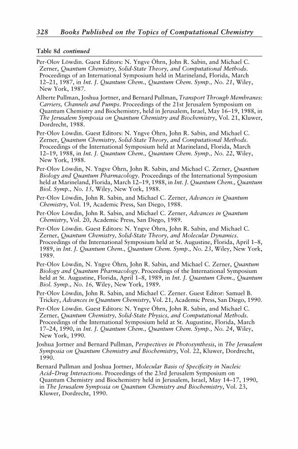
Table 8d continued

Per-Olov Lowdin. Guest Editors: N. Yngve Ohrn, John R. Sabin, and Michael C.Zerner, Quantum Chemistry, Solid-State Theory, and Computational Methods.Proceedings of an International Symposium held in Marineland, Florida, March12–21, 1987, in Int. J. Quantum Chem., Quantum Chem. Symp., No. 21, Wiley,New York, 1987.

Alberte Pullman, Joshua Jortner, and Bernard Pullman, Transport Through Membranes:Carriers, Channels and Pumps. Proceedings of the 21st Jerusalem Symposium onQuantum Chemistry and Biochemistry, held in Jerusalem, Israel, May 16–19, 1988, inThe Jerusalem Symposia on Quantum Chemistry and Biochemistry, Vol. 21, Kluwer,Dordrecht, 1988.

Per-Olov Lowdin. Guest Editors: N. Yngve Ohrn, John R. Sabin, and Michael C.Zerner, Quantum Chemistry, Solid-State Theory, and Computational Methods.Proceedings of the International Symposium held at Marineland, Florida, March12–19, 1988, in Int. J. Quantum Chem., Quantum Chem. Symp., No. 22, Wiley,New York, 1988.

Per-Olov Lowdin, N. Yngve Ohrn, John R. Sabin, and Michael C. Zerner, QuantumBiology and Quantum Pharmacology. Proceedings of the International Symposiumheld at Marineland, Florida, March 12–19, 1988, in Int. J. Quantum Chem., QuantumBiol. Symp., No. 15, Wiley, New York, 1988.

Per-Olov Lowdin, John R. Sabin, and Michael C. Zerner, Advances in QuantumChemistry, Vol. 19, Academic Press, San Diego, 1988.

Per-Olov Lowdin, John R. Sabin, and Michael C. Zerner, Advances in QuantumChemistry, Vol. 20, Academic Press, San Diego, 1989.

Per-Olov Lowdin. Guest Editors: N. Yngve Ohrn, John R. Sabin, and Michael C.Zerner, Quantum Chemistry, Solid-State Theory, and Molecular Dynamics.Proceedings of the International Symposium held at St. Augustine, Florida, April 1–8,1989, in Int. J. Quantum Chem., Quantum Chem. Symp., No. 23, Wiley, New York,1989.

Per-Olov Lowdin, N. Yngve Ohrn, John R. Sabin, and Michael C. Zerner, QuantumBiology and Quantum Pharmacology. Proceedings of the International Symposiumheld at St. Augustine, Florida, April 1–8, 1989, in Int. J. Quantum Chem., QuantumBiol. Symp., No. 16, Wiley, New York, 1989.

Per-Olov Lowdin, John R. Sabin, and Michael C. Zerner. Guest Editor: Samuel B.Trickey, Advances in Quantum Chemistry, Vol. 21, Academic Press, San Diego, 1990.

Per-Olov Lowdin. Guest Editors: N. Yngve Ohrn, John R. Sabin, and Michael C.Zerner, Quantum Chemistry, Solid-State Physics, and Computational Methods.Proceedings of the International Symposium held at St. Augustine, Florida, March17–24, 1990, in Int. J. Quantum Chem., Quantum Chem. Symp., No. 24, Wiley,New York, 1990.

Joshua Jortner and Bernard Pullman, Perspectives in Photosynthesis, in The JerusalemSymposia on Quantum Chemistry and Biochemistry, Vol. 22, Kluwer, Dordrecht,1990.

Bernard Pullman and Joshua Jortner, Molecular Basis of Specificity in NucleicAcid–Drug Interactions. Proceedings of the 23rd Jerusalem Symposium onQuantum Chemistry and Biochemistry held in Jerusalem, Israel, May 14–17, 1990,in The Jerusalem Symposia on Quantum Chemistry and Biochemistry, Vol. 23,Kluwer, Dordrecht, 1990.

328 Books Published on the Topics of Computational Chemistry

Table 8d continued

Per-Olov Lowdin, N. Yngve Ohrn, John R. Sabin, and Michael C. Zerner, QuantumBiology and Quantum Pharmacology. Proceedings of the International Symposiumheld at St. Augustine, Florida, March 17–24, 1990, in Int. J. Quantum Chem.,Quantum Biol. Symp., No. 17, Wiley, New York, 1990.

Per-Olov Lowdin. Guest Editors: N. Yngve Ohrn, John R. Sabin, and Michael C.Zerner, Quantum Chemistry, Solid-State Theory, and Molecular Dynamics. Pro-ceedings of the International Symposium held at St. Augustine, Florida, March 9–16,1991, in Int. J. Quantum Chem., Quantum Chem. Symp., No. 25, Wiley, New York,1991.

Per-Olov Lowdin, N. Yngve Ohrn, John R. Sabin, and Michael C. Zerner, QuantumBiology and Quantum Pharmacology. Proceedings of the International Symposiumheld at St. Augustine, Florida, March 9–16, 1991, in Int. J. Quantum Chem., QuantumBiol. Symp., No. 18, Wiley, New York, 1991.

Per-Olov Lowdin, John R. Sabin, and Michael C. Zerner, Advances in QuantumChemistry, Vol. 22, Academic Press, San Diego, 1991.

Joshua Jortner, R. D. Levine, and B. Pullman, Mode Selective Chemistry. Proceedings ofthe 24th Jerusalem Symposium on Quantum Chemistry and Biochemistry held inJerusalem, Israel, May 20–23, 1991, in The Jerusalem Symposia on QuantumChemistry and Biochemistry, Vol. 24, Kluwer, Dordrecht, 1991.

Alberte Pullman, Joshua Jortner, and Bernard Pullman, Membrane Proteins: Structures,Interactions and Models. Proceedings of the 25th Jerusalem Symposium on QuantumChemistry and Biochemistry held in Jerusalem, Israel, May 18–21, 1992, in JerusalemSymposia on Quantum Chemistry and Biochemistry, Vol. 25, Kluwer, Dordrecht,1992.

Per-Olov Lowdin, N. Yngve Ohrn, John R. Sabin, and Michael C. Zerner, Applicationof Fundamental Theory to Quantum Biology and Quantum Pharmacology. Proceed-ings of the International Symposium held at St. Augustine, Florida, March 14–21,1992, in Int. J. Quantum Chem., Quantum Biol. Symp., No. 19, Wiley, New York,1992.

Per-Olov Lowdin. Guest Editors: N. Yngve Ohrn, John R. Sabin, and Michael C.Zerner, Atomic, Molecular, and Condensed Matter Theory and ComputationalMethods. Proceedings of the International Symposium held at St. Augustine, Florida,March 14–21, 1992, in Int. J. Quantum Chem., Quantum Chem. Symp., No. 26,Wiley, New York, 1992.

Per-Olov Lowdin, John R. Sabin, and Michael C. Zerner, Advances in QuantumChemistry, Vol. 23, Academic Press, San Diego, 1992.

Per-Olov Lowdin, John R. Sabin, and Michael C. Zerner, Advances in QuantumChemistry, Vol. 24, Academic Press, San Diego, 1992.

Per-Olov Lowdin. Guest editors: N. Yngve Ohrn, John R. Sabin, and Michael C. Zerner,Atomic, Molecular, and Condensed Matter Theory and Computational Methods.Proceedings of the International Symposium held at St. Augustine, Florida, March13–20, 1993, in Int. J. Quantum Chem., Quantum Chem. Symp., No. 27, Wiley,New York, 1993.

Per-Olov Lowdin, N. Yngve Ohrn, John R. Sabin, and Michael C. Zerner, Applicationof Fundamental Theory to Problems of Biology and Pharmacology. Proceedings of theInternational Symposium held at St. Augustine, Florida, March 13–20, 1993, in Int. J.Quantum Chem., Quantum Biol. Symp., No. 20, Wiley, New York, 1993.

Quantum Chemistry 329

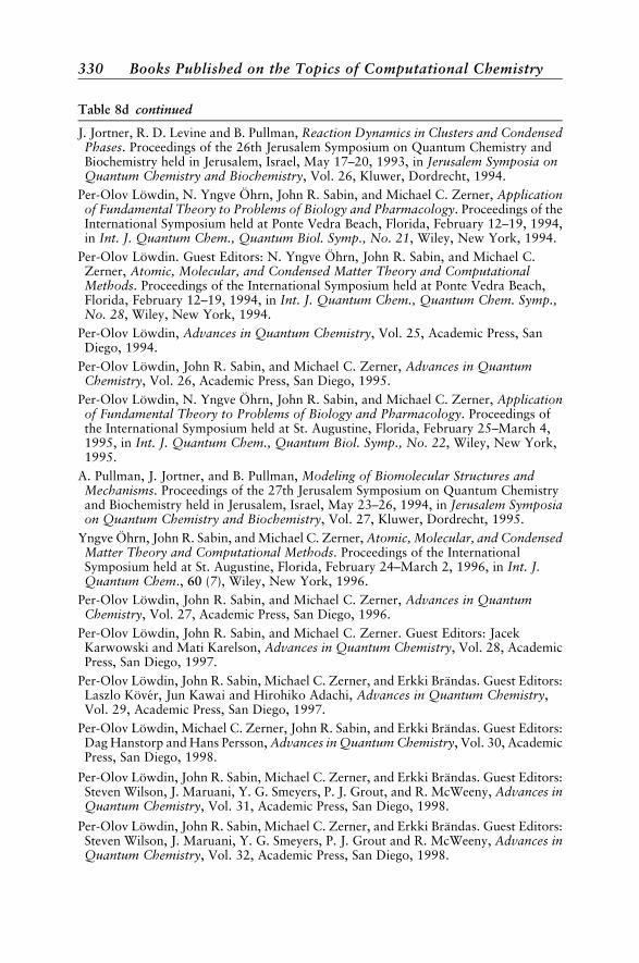
Table 8d continued

J. Jortner, R. D. Levine and B. Pullman, Reaction Dynamics in Clusters and CondensedPhases. Proceedings of the 26th Jerusalem Symposium on Quantum Chemistry andBiochemistry held in Jerusalem, Israel, May 17–20, 1993, in Jerusalem Symposia onQuantum Chemistry and Biochemistry, Vol. 26, Kluwer, Dordrecht, 1994.

Per-Olov Lowdin, N. Yngve Ohrn, John R. Sabin, and Michael C. Zerner, Applicationof Fundamental Theory to Problems of Biology and Pharmacology. Proceedings of theInternational Symposium held at Ponte Vedra Beach, Florida, February 12–19, 1994,in Int. J. Quantum Chem., Quantum Biol. Symp., No. 21, Wiley, New York, 1994.

Per-Olov Lowdin. Guest Editors: N. Yngve Ohrn, John R. Sabin, and Michael C.Zerner, Atomic, Molecular, and Condensed Matter Theory and ComputationalMethods. Proceedings of the International Symposium held at Ponte Vedra Beach,Florida, February 12–19, 1994, in Int. J. Quantum Chem., Quantum Chem. Symp.,No. 28, Wiley, New York, 1994.

Per-Olov Lowdin, Advances in Quantum Chemistry, Vol. 25, Academic Press, SanDiego, 1994.

Per-Olov Lowdin, John R. Sabin, and Michael C. Zerner, Advances in QuantumChemistry, Vol. 26, Academic Press, San Diego, 1995.

Per-Olov Lowdin, N. Yngve Ohrn, John R. Sabin, and Michael C. Zerner, Applicationof Fundamental Theory to Problems of Biology and Pharmacology. Proceedings ofthe International Symposium held at St. Augustine, Florida, February 25–March 4,1995, in Int. J. Quantum Chem., Quantum Biol. Symp., No. 22, Wiley, New York,1995.

A. Pullman, J. Jortner, and B. Pullman, Modeling of Biomolecular Structures andMechanisms. Proceedings of the 27th Jerusalem Symposium on Quantum Chemistryand Biochemistry held in Jerusalem, Israel, May 23–26, 1994, in Jerusalem Symposiaon Quantum Chemistry and Biochemistry, Vol. 27, Kluwer, Dordrecht, 1995.

Yngve Ohrn, John R. Sabin, and Michael C. Zerner, Atomic, Molecular, and CondensedMatter Theory and Computational Methods. Proceedings of the InternationalSymposium held at St. Augustine, Florida, February 24–March 2, 1996, in Int. J.Quantum Chem., 60 (7), Wiley, New York, 1996.

Per-Olov Lowdin, John R. Sabin, and Michael C. Zerner, Advances in QuantumChemistry, Vol. 27, Academic Press, San Diego, 1996.

Per-Olov Lowdin, John R. Sabin, and Michael C. Zerner. Guest Editors: JacekKarwowski and Mati Karelson, Advances in Quantum Chemistry, Vol. 28, AcademicPress, San Diego, 1997.

Per-Olov Lowdin, John R. Sabin, Michael C. Zerner, and Erkki Brandas. Guest Editors:Laszlo Kover, Jun Kawai and Hirohiko Adachi, Advances in Quantum Chemistry,Vol. 29, Academic Press, San Diego, 1997.

Per-Olov Lowdin, Michael C. Zerner, John R. Sabin, and Erkki Brandas. Guest Editors:Dag Hanstorp and Hans Persson, Advances in Quantum Chemistry, Vol. 30, AcademicPress, San Diego, 1998.

Per-Olov Lowdin, John R. Sabin, Michael C. Zerner, and Erkki Brandas. Guest Editors:Steven Wilson, J. Maruani, Y. G. Smeyers, P. J. Grout, and R. McWeeny, Advances inQuantum Chemistry, Vol. 31, Academic Press, San Diego, 1998.

Per-Olov Lowdin, John R. Sabin, Michael C. Zerner, and Erkki Brandas. Guest Editors:Steven Wilson, J. Maruani, Y. G. Smeyers, P. J. Grout and R. McWeeny, Advances inQuantum Chemistry, Vol. 32, Academic Press, San Diego, 1998.

330 Books Published on the Topics of Computational Chemistry

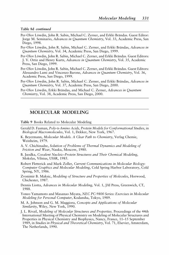
Table 8d continued

Per-Olov Lowdin, John R. Sabin, Michael C. Zerner, and Erkki Brandas. Guest Editor:Jorge M. Seminario, Advances in Quantum Chemistry, Vol. 33, Academic Press, SanDiego, 1998.

Per-Olov Lowdin, John R. Sabin, Michael C. Zerner, and Erkki Brandas, Advances inQuantum Chemistry, Vol. 34, Academic Press, San Diego, 1999.

Per-Olov Lowdin, John R. Sabin, Michael C. Zerner, and Erkki Brandas. Guest Editors:J. V. Ortiz and Henry Kurtz, Advances in Quantum Chemistry, Vol. 35, AcademicPress, San Diego, 1999.

Per-Olov Lowdin, John R. Sabin, Michael C. Zerner, and Erkki Brandas. Guest Editors:Alessandro Lami and Vincenzo Barone, Advances in Quantum Chemistry, Vol. 36,Academic Press, San Diego, 1999.

Per-Olov Lowdin, John R. Sabin, Michael C. Zerner, and Erkki Brandas, Advances inQuantum Chemistry, Vol. 37, Academic Press, San Diego, 2000.

Per-Olov Lowdin, Erkki Brandas, and Michael C. Zerner, Advances in QuantumChemistry, Vol. 38, Academic Press, San Diego, 2000.

MOLECULAR MODELING

Table 9 Books Related to Molecular Modeling

Gerald D. Fasman, Poly-a-Amino Acids, Protein Models for Conformational Studies, inBiological Macromolecules, Vol. 1, Dekker, New York, 1967.

K. Beyermann, Molecular Models. A Clear Path to Chemistry, Verlag Chemie,Weinheim, 1979.

A. V. Chichinadze, Solution of Problems of Thermal Dynamics and Modeling ofFriction and Wear, Nauka, Moscow, 1980.

B. Juodka, Covalent Nucleic–Protein Structures and Their Chemical Modeling,Mokslas, Vilnius, USSR, 1985.

Robert Fletterick and Mark Zoller, Current Communications in Molecular Biology:Computer Graphics and Molecular Modeling, Cold Spring Harbor Laboratory, ColdSpring, NY, 1986.

Zvonimir B. Maksic, Modeling of Structure and Properties of Molecules, Horwood,Chichester, 1987.

Dennis Liotta, Advances in Molecular Modeling, Vol. 1, JAI Press, Greenwich, CT,1988.

Yoneo Yamamoto and Masanao Miyata, NEC PC-9800 Series: Exercises in MolecularModeling for Personal Computer, Kodansha, Tokyo, 1989.

M. A. Johnson and G. M. Maggiora, Concepts and Applications of MolecularSimilarity, Wiley, New York, 1990.

J. L. Rivail, Modeling of Molecular Structures and Properties. Proceedings of the 44thInternational Meeting of Physical Chemistry on Modeling of Molecular Structures andProperties in Physical Chemistry and Biophysics, Nancy, France, 11–15 September1989, in Studies in Physical and Theoretical Chemistry, Vol. 71, Elsevier, Amsterdam,The Netherlands, 1990.

Molecular Modeling 331

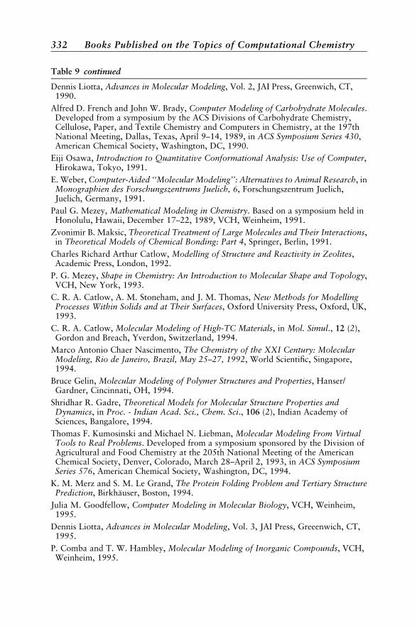
Table 9 continued

Dennis Liotta, Advances in Molecular Modeling, Vol. 2, JAI Press, Greenwich, CT,1990.

Alfred D. French and John W. Brady, Computer Modeling of Carbohydrate Molecules.Developed from a symposium by the ACS Divisions of Carbohydrate Chemistry,Cellulose, Paper, and Textile Chemistry and Computers in Chemistry, at the 197thNational Meeting, Dallas, Texas, April 9–14, 1989, in ACS Symposium Series 430,American Chemical Society, Washington, DC, 1990.

Eiji Osawa, Introduction to Quantitative Conformational Analysis: Use of Computer,Hirokawa, Tokyo, 1991.

E. Weber, Computer-Aided ‘‘Molecular Modeling’’: Alternatives to Animal Research, inMonographien des Forschungszentrums Juelich, 6, Forschungszentrum Juelich,Juelich, Germany, 1991.

Paul G. Mezey, Mathematical Modeling in Chemistry. Based on a symposium held inHonolulu, Hawaii, December 17–22, 1989, VCH, Weinheim, 1991.

Zvonimir B. Maksic, Theoretical Treatment of Large Molecules and Their Interactions,in Theoretical Models of Chemical Bonding: Part 4, Springer, Berlin, 1991.

Charles Richard Arthur Catlow, Modelling of Structure and Reactivity in Zeolites,Academic Press, London, 1992.

P. G. Mezey, Shape in Chemistry: An Introduction to Molecular Shape and Topology,VCH, New York, 1993.

C. R. A. Catlow, A. M. Stoneham, and J. M. Thomas, New Methods for ModellingProcesses Within Solids and at Their Surfaces, Oxford University Press, Oxford, UK,1993.

C. R. A. Catlow, Molecular Modeling of High-TC Materials, in Mol. Simul., 12 (2),Gordon and Breach, Yverdon, Switzerland, 1994.

Marco Antonio Chaer Nascimento, The Chemistry of the XXI Century: MolecularModeling, Rio de Janeiro, Brazil, May 25–27, 1992, World Scientific, Singapore,1994.

Bruce Gelin, Molecular Modeling of Polymer Structures and Properties, Hanser/Gardner, Cincinnati, OH, 1994.

Shridhar R. Gadre, Theoretical Models for Molecular Structure Properties andDynamics, in Proc. - Indian Acad. Sci., Chem. Sci., 106 (2), Indian Academy ofSciences, Bangalore, 1994.

Thomas F. Kumosinski and Michael N. Liebman, Molecular Modeling From VirtualTools to Real Problems. Developed from a symposium sponsored by the Division ofAgricultural and Food Chemistry at the 205th National Meeting of the AmericanChemical Society, Denver, Colorado, March 28–April 2, 1993, in ACS SymposiumSeries 576, American Chemical Society, Washington, DC, 1994.

K. M. Merz and S. M. Le Grand, The Protein Folding Problem and Tertiary StructurePrediction, Birkhauser, Boston, 1994.

Julia M. Goodfellow, Computer Modeling in Molecular Biology, VCH, Weinheim,1995.

Dennis Liotta, Advances in Molecular Modeling, Vol. 3, JAI Press, Greeenwich, CT,1995.

P. Comba and T. W. Hambley, Molecular Modeling of Inorganic Compounds, VCH,Weinheim, 1995.

332 Books Published on the Topics of Computational Chemistry

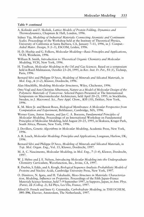
Table 9 continued

A. Kolinski and F. Skolnik, Lattice Models of Protein Folding, Dynamics andThermodynamics, Chapman & Hall, London, 1996.

Sidney Yip, Modeling of Industrial Materials: Connecting Atomistic and ContinuumScales. Proceedings of the Workshop held at the Institute of Theoretical Physics,University of California at Santa Barbara, CA, January 7–11, 1996, in J. Comput.-Aided Mater. Design, 3 (1–3), ESCOM, Leiden, 1996.

H.-D. Hoeltje and G. Folkers, Molecular Modeling—Basic Principles and Applications,VCH, Weinheim, 1996.

William B. Smith, Introduction to Theoretical Organic Chemistry and MolecularModeling, VCH, New York, 1996.

H. Toulhoat, Molecular Modeling in the Oil and Gas Sciences. Based on a symposiumheld in Rueil-Malmaison, October 23–24, 1995, in Rev. Inst. Fr. Pet., 51 (1), Technip,Paris, 1996.

Bernard Silvi and Philippe D’Arco, Modeling of Minerals and Silicated Materials, inMol. Eng., 6 (1–2), Kluwer, Dordrecht, 1996.

Alan Hinchliffe, Modeling Molecular Structures, Wiley, Chichester, 1996.

Otto Vogl and Ann-Christine Albertsson, Nature as a Model of Molecular Design of thePolymeric Materials of Tomorrow. Selected Papers Presented at The InternationalSymposium on Macromolecular Architecture, held April 20–21, 1995, in Stockholm,Sweden, in J. Macromol. Sci., Pure Appl. Chem., A33 (10), Dekker, New York,1996.

K. M. Merz Jr. and Benoit Roux, Biological Membranes: A Molecular Perspective fromComputation and Experiment, Birkhauser, Cambridge, MA, 1996.

Werner Gans, Anton Amann, and Jan C. A. Boeyens, Fundamental Principles ofMolecular Modeling. Proceedings of an International Workshop on FundamentalPrinciples of Molecular Modeling, held August 20–25, 1995, in Skukuza, Kruger Park,South Africa, Plenum, New York, 1996.

J. Devillers, Genetic Algorithms in Molecular Modeling, Academic Press, New York,1996.

A. R. Leach, Molecular Modeling: Principles and Applications, Longman, Harlow, UK,1996.

Bernard Silvi and Philippe D’Arco, Modeling of Minerals and Silicated Materials, inTop. Mol. Organ. Eng., Vol. 15, Kluwer, Dordrecht, 1997.

M. A. C. Nascimento, Molecular Modeling, in Mol. Eng., 7 (3–4), Kluwer, Dordrecht,1997.

W. J. Hehre and J. E. Nelson, Introducing Molecular Modeling into the UndergraduateChemistry Curriculum, Wavefunction, Inc., Irvine, CA, 1997.

R. Durbin, S. Eddy, and A. Krogh, Biological Sequence Analysis: Probabilistic Models ofProteins and Nucleic Acids, Cambridge University Press, New York, 1997.

O. Dimitrov, N. Igata, and H. Takahashi, Meso-Structure in Materials: Characteriza-tion, Modeling, Influence on Properties. Proceedings of the Fifth Japan–FranceMaterials Science Seminar, held 7–9 September 1997, in Sapporo, Japan, in Ann. Phys.(Paris), 22 (Colloq. 2), Ed Phys, Les Ulis, France, 1997.

Alfred D. French and Imre G. Csizmadia, Carbohydrate Modeling, in THEOCHEM,395–396, Elsevier, Amsterdam, The Netherlands, 1997.

Molecular Modeling 333

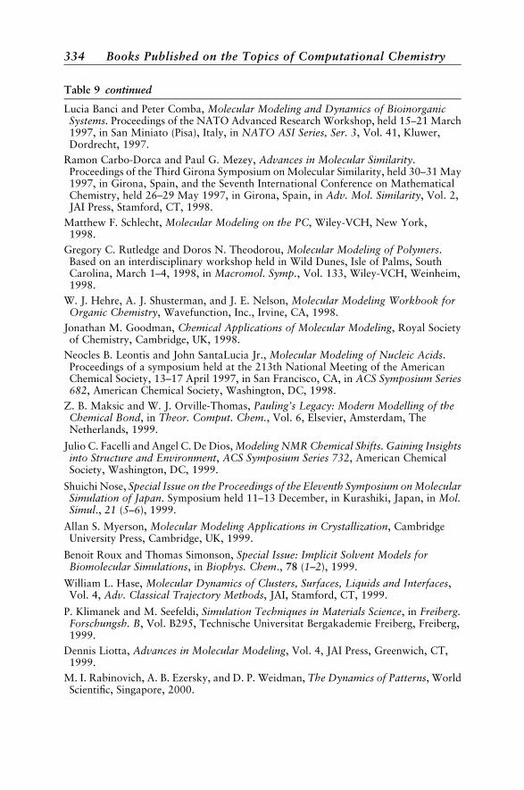
Table 9 continued

Lucia Banci and Peter Comba, Molecular Modeling and Dynamics of BioinorganicSystems. Proceedings of the NATO Advanced Research Workshop, held 15–21 March1997, in San Miniato (Pisa), Italy, in NATO ASI Series, Ser. 3, Vol. 41, Kluwer,Dordrecht, 1997.

Ramon Carbo-Dorca and Paul G. Mezey, Advances in Molecular Similarity.Proceedings of the Third Girona Symposium on Molecular Similarity, held 30–31 May1997, in Girona, Spain, and the Seventh International Conference on MathematicalChemistry, held 26–29 May 1997, in Girona, Spain, in Adv. Mol. Similarity, Vol. 2,JAI Press, Stamford, CT, 1998.

Matthew F. Schlecht, Molecular Modeling on the PC, Wiley-VCH, New York,1998.

Gregory C. Rutledge and Doros N. Theodorou, Molecular Modeling of Polymers.Based on an interdisciplinary workshop held in Wild Dunes, Isle of Palms, SouthCarolina, March 1–4, 1998, in Macromol. Symp., Vol. 133, Wiley-VCH, Weinheim,1998.

W. J. Hehre, A. J. Shusterman, and J. E. Nelson, Molecular Modeling Workbook forOrganic Chemistry, Wavefunction, Inc., Irvine, CA, 1998.

Jonathan M. Goodman, Chemical Applications of Molecular Modeling, Royal Societyof Chemistry, Cambridge, UK, 1998.

Neocles B. Leontis and John SantaLucia Jr., Molecular Modeling of Nucleic Acids.Proceedings of a symposium held at the 213th National Meeting of the AmericanChemical Society, 13–17 April 1997, in San Francisco, CA, in ACS Symposium Series682, American Chemical Society, Washington, DC, 1998.

Z. B. Maksic and W. J. Orville-Thomas, Pauling’s Legacy: Modern Modelling of theChemical Bond, in Theor. Comput. Chem., Vol. 6, Elsevier, Amsterdam, TheNetherlands, 1999.

Julio C. Facelli and Angel C. De Dios, Modeling NMR Chemical Shifts. Gaining Insightsinto Structure and Environment, ACS Symposium Series 732, American ChemicalSociety, Washington, DC, 1999.

Shuichi Nose, Special Issue on the Proceedings of the Eleventh Symposium on MolecularSimulation of Japan. Symposium held 11–13 December, in Kurashiki, Japan, in Mol.Simul., 21 (5–6), 1999.

Allan S. Myerson, Molecular Modeling Applications in Crystallization, CambridgeUniversity Press, Cambridge, UK, 1999.

Benoit Roux and Thomas Simonson, Special Issue: Implicit Solvent Models forBiomolecular Simulations, in Biophys. Chem., 78 (1–2), 1999.

William L. Hase, Molecular Dynamics of Clusters, Surfaces, Liquids and Interfaces,Vol. 4, Adv. Classical Trajectory Methods, JAI, Stamford, CT, 1999.

P. Klimanek and M. Seefeldi, Simulation Techniques in Materials Science, in Freiberg.Forschungsh. B, Vol. B295, Technische Universitat Bergakademie Freiberg, Freiberg,1999.

Dennis Liotta, Advances in Molecular Modeling, Vol. 4, JAI Press, Greenwich, CT,1999.

M. I. Rabinovich, A. B. Ezersky, and D. P. Weidman, The Dynamics of Patterns, WorldScientific, Singapore, 2000.

334 Books Published on the Topics of Computational Chemistry

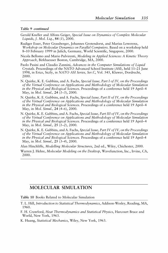
Table 9 continued

Gerald Kneller and Alfons Geiger, Special Issue on Dynamics of Complex MolecularLiquids, J. Mol. Liq., 84 (1), 2000.

Rudiger Esser, Peter Grassberger, Johannes Grotendorst, and Marius Lewerenz,Workshop on Molecular Dynamics on Parallel Computers. Based on a workshop held8–10 February 1999 in Julich, Germany, World Scientific, Singapore, 2000.

Nicola Bellomo and Mario Pulvirenti, Modeling in Applied Sciences: A Kinetic TheoryApproach, Birkhaeuser Boston, Cambridge, MA, 2000.

Paolo Pasini and Claudio Zannini, Advances in the Computer Simulations of LiquidCrystals. Proceedings of the NATO Advanced School Institute (ASI), held 11–21 June1998, in Erice, Sicily, in NATO ASI Series, Ser.C, Vol. 545, Kluwer, Dordrecht,2000.

N. Quirke, K. E. Gubbins, and A. Fuchs, Special Issue, Part I of IV, on the Proceedingsof the Virtual Conference on Applications and Methodology of Molecular Simulationin the Physical and Biological Sciences. Proceedings of a conference held 19 April–4May, in Mol. Simul., 24 (1–3), 2000.

N. Quirke, K. E. Gubbins, and A. Fuchs, Special Issue, Part II of IV, on the Proceedingsof the Virtual Conference on Applications and Methodology of Molecular Simulationin the Physical and Biological Sciences. Proceedings of a conference held 19 April–4May, in Mol. Simul., 24 (4–6), 2000.

N. Quirke, K. E. Gubbins, and A. Fuchs, Special Issue, Part III of IV, on the Proceedingsof the Virtual Conference on Applications and Methodology of Molecular Simulationin the Physical and Biological Sciences. Proceedings of a conference held 19 April–4May, in Mol. Simul., 25 (1–2), 2000.

N. Quirke, K. E. Gubbins, and A. Fuchs, Special Issue, Part IV of IV, on the Proceedingsof the Virtual Conference on Applications and Methodology of Molecular Simulationin the Physical and Biological Sciences. Proceedings of a conference held 19 April–4May, in Mol. Simul., 25 (3–4), 2000.

Alan Hinchliffe, Modelling Molecular Structures, 2nd ed., Wiley, Chichester, 2000.

Warren J. Hehre, Molecular Modeling on the Desktop, Wavefunction, Inc., Irvine, CA,2000.

MOLECULAR SIMULATION

Table 10 Books Related to Molecular Simulation

T. L. Hill, Introduction to Statistical Thermodynamics, Addison-Wesley, Reading, MA,1960.

F. H. Crawford, Heat Thermodynamics and Statistical Physics, Harcourt Brace andWorld, New York, 1963.

K. Huang, Statistical Mechanics, Wiley, New York, 1963.

Molecular Simulation 335

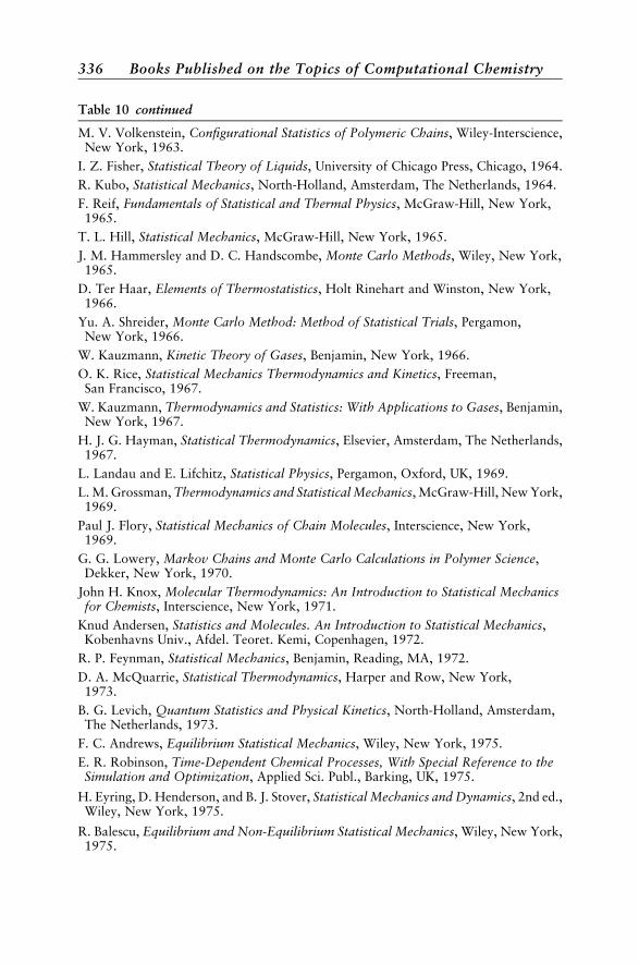
Table 10 continued

M. V. Volkenstein, Configurational Statistics of Polymeric Chains, Wiley-Interscience,New York, 1963.

I. Z. Fisher, Statistical Theory of Liquids, University of Chicago Press, Chicago, 1964.

R. Kubo, Statistical Mechanics, North-Holland, Amsterdam, The Netherlands, 1964.

F. Reif, Fundamentals of Statistical and Thermal Physics, McGraw-Hill, New York,1965.

T. L. Hill, Statistical Mechanics, McGraw-Hill, New York, 1965.

J. M. Hammersley and D. C. Handscombe, Monte Carlo Methods, Wiley, New York,1965.

D. Ter Haar, Elements of Thermostatistics, Holt Rinehart and Winston, New York,1966.

Yu. A. Shreider, Monte Carlo Method: Method of Statistical Trials, Pergamon,New York, 1966.

W. Kauzmann, Kinetic Theory of Gases, Benjamin, New York, 1966.

O. K. Rice, Statistical Mechanics Thermodynamics and Kinetics, Freeman,San Francisco, 1967.

W. Kauzmann, Thermodynamics and Statistics: With Applications to Gases, Benjamin,New York, 1967.

H. J. G. Hayman, Statistical Thermodynamics, Elsevier, Amsterdam, The Netherlands,1967.

L. Landau and E. Lifchitz, Statistical Physics, Pergamon, Oxford, UK, 1969.

L. M. Grossman, Thermodynamics and Statistical Mechanics, McGraw-Hill, New York,1969.

Paul J. Flory, Statistical Mechanics of Chain Molecules, Interscience, New York,1969.

G. G. Lowery, Markov Chains and Monte Carlo Calculations in Polymer Science,Dekker, New York, 1970.

John H. Knox, Molecular Thermodynamics: An Introduction to Statistical Mechanicsfor Chemists, Interscience, New York, 1971.

Knud Andersen, Statistics and Molecules. An Introduction to Statistical Mechanics,Kobenhavns Univ., Afdel. Teoret. Kemi, Copenhagen, 1972.

R. P. Feynman, Statistical Mechanics, Benjamin, Reading, MA, 1972.

D. A. McQuarrie, Statistical Thermodynamics, Harper and Row, New York,1973.

B. G. Levich, Quantum Statistics and Physical Kinetics, North-Holland, Amsterdam,The Netherlands, 1973.

F. C. Andrews, Equilibrium Statistical Mechanics, Wiley, New York, 1975.

E. R. Robinson, Time-Dependent Chemical Processes, With Special Reference to theSimulation and Optimization, Applied Sci. Publ., Barking, UK, 1975.

H. Eyring, D. Henderson, and B. J. Stover, Statistical Mechanics and Dynamics, 2nd ed.,Wiley, New York, 1975.

R. Balescu, Equilibrium and Non-Equilibrium Statistical Mechanics, Wiley, New York,1975.

336 Books Published on the Topics of Computational Chemistry

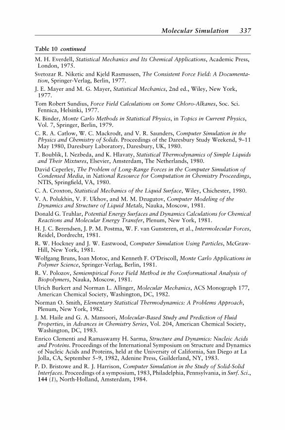
Table 10 continued

M. H. Everdell, Statistical Mechanics and Its Chemical Applications, Academic Press,London, 1975.

Svetozar R. Niketic and Kjeld Rasmussen, The Consistent Force Field: A Documenta-tion, Springer-Verlag, Berlin, 1977.

J. E. Mayer and M. G. Mayer, Statistical Mechanics, 2nd ed., Wiley, New York,1977.

Tom Robert Sundius, Force Field Calculations on Some Chloro-Alkanes, Soc. Sci.Fennica, Helsinki, 1977.

K. Binder, Monte Carlo Methods in Statistical Physics, in Topics in Current Physics,Vol. 7, Springer, Berlin, 1979.

C. R. A. Catlow, W. C. Mackrodt, and V. R. Saunders, Computer Simulation in thePhysics and Chemistry of Solids. Proceedings of the Daresbury Study Weekend, 9–11May 1980, Daresbury Laboratory, Daresbury, UK, 1980.

T. Boublik, I. Nezbeda, and K. Hlavaty, Statistical Thermodynamics of Simple Liquidsand Their Mixtures, Elsevier, Amsterdam, The Netherlands, 1980.

David Ceperley, The Problem of Long-Range Forces in the Computer Simulation ofCondensed Media, in National Resource for Computation in Chemistry Proceedings,NTIS, Springfield, VA, 1980.

C. A. Croxton, Statistical Mechanics of the Liquid Surface, Wiley, Chichester, 1980.

V. A. Polukhin, V. F. Ukhov, and M. M. Dzugutov, Computer Modeling of theDynamics and Structure of Liquid Metals, Nauka, Moscow, 1981.

Donald G. Truhlar, Potential Energy Surfaces and Dynamics Calculations for ChemicalReactions and Molecular Energy Transfer, Plenum, New York, 1981.

H. J. C. Berendsen, J. P. M. Postma, W. F. van Gunsteren, et al., Intermolecular Forces,Reidel, Dordrecht, 1981.

R. W. Hockney and J. W. Eastwood, Computer Simulation Using Particles, McGraw-Hill, New York, 1981.

Wolfgang Bruns, Ioan Motoc, and Kenneth F. O’Driscoll, Monte Carlo Applications inPolymer Science, Springer-Verlag, Berlin, 1981.

R. V. Polozov, Semiempirical Force Field Method in the Conformational Analysis ofBiopolymers, Nauka, Moscow, 1981.

Ulrich Burkert and Norman L. Allinger, Molecular Mechanics, ACS Monograph 177,American Chemical Society, Washington, DC, 1982.

Norman O. Smith, Elementary Statistical Thermodynamics: A Problems Approach,Plenum, New York, 1982.

J. M. Haile and G. A. Mansoori, Molecular-Based Study and Prediction of FluidProperties, in Advances in Chemistry Series, Vol. 204, American Chemical Society,Washington, DC, 1983.

Enrico Clementi and Ramaswamy H. Sarma, Structure and Dynamics: Nucleic Acidsand Proteins. Proceedings of the International Symposium on Structure and Dynamicsof Nucleic Acids and Proteins, held at the University of California, San Diego at LaJolla, CA, September 5–9, 1982, Adenine Press, Guilderland, NY, 1983.

P. D. Bristowe and R. J. Harrison, Computer Simulation in the Study of Solid-SolidInterfaces. Proceedings of a symposium, 1983, Philadelphia, Pennsylvania, in Surf. Sci.,144 (1), North-Holland, Amsterdam, 1984.

Molecular Simulation 337

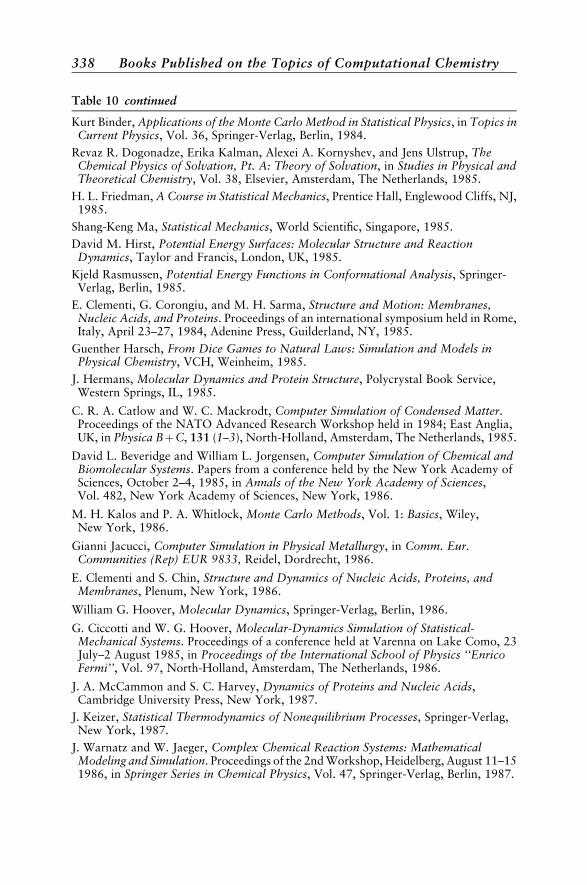
Table 10 continued

Kurt Binder, Applications of the Monte Carlo Method in Statistical Physics, in Topics inCurrent Physics, Vol. 36, Springer-Verlag, Berlin, 1984.

Revaz R. Dogonadze, Erika Kalman, Alexei A. Kornyshev, and Jens Ulstrup, TheChemical Physics of Solvation, Pt. A: Theory of Solvation, in Studies in Physical andTheoretical Chemistry, Vol. 38, Elsevier, Amsterdam, The Netherlands, 1985.

H. L. Friedman, A Course in Statistical Mechanics, Prentice Hall, Englewood Cliffs, NJ,1985.

Shang-Keng Ma, Statistical Mechanics, World Scientific, Singapore, 1985.

David M. Hirst, Potential Energy Surfaces: Molecular Structure and ReactionDynamics, Taylor and Francis, London, UK, 1985.

Kjeld Rasmussen, Potential Energy Functions in Conformational Analysis, Springer-Verlag, Berlin, 1985.

E. Clementi, G. Corongiu, and M. H. Sarma, Structure and Motion: Membranes,Nucleic Acids, and Proteins. Proceedings of an international symposium held in Rome,Italy, April 23–27, 1984, Adenine Press, Guilderland, NY, 1985.

Guenther Harsch, From Dice Games to Natural Laws: Simulation and Models inPhysical Chemistry, VCH, Weinheim, 1985.

J. Hermans, Molecular Dynamics and Protein Structure, Polycrystal Book Service,Western Springs, IL, 1985.

C. R. A. Catlow and W. C. Mackrodt, Computer Simulation of Condensed Matter.Proceedings of the NATO Advanced Research Workshop held in 1984; East Anglia,UK, in Physica BþC, 131 (1–3), North-Holland, Amsterdam, The Netherlands, 1985.

David L. Beveridge and William L. Jorgensen, Computer Simulation of Chemical andBiomolecular Systems. Papers from a conference held by the New York Academy ofSciences, October 2–4, 1985, in Annals of the New York Academy of Sciences,Vol. 482, New York Academy of Sciences, New York, 1986.

M. H. Kalos and P. A. Whitlock, Monte Carlo Methods, Vol. 1: Basics, Wiley,New York, 1986.

Gianni Jacucci, Computer Simulation in Physical Metallurgy, in Comm. Eur.Communities (Rep) EUR 9833, Reidel, Dordrecht, 1986.

E. Clementi and S. Chin, Structure and Dynamics of Nucleic Acids, Proteins, andMembranes, Plenum, New York, 1986.

William G. Hoover, Molecular Dynamics, Springer-Verlag, Berlin, 1986.

G. Ciccotti and W. G. Hoover, Molecular-Dynamics Simulation of Statistical-Mechanical Systems. Proceedings of a conference held at Varenna on Lake Como, 23July–2 August 1985, in Proceedings of the International School of Physics ‘‘EnricoFermi’’, Vol. 97, North-Holland, Amsterdam, The Netherlands, 1986.

J. A. McCammon and S. C. Harvey, Dynamics of Proteins and Nucleic Acids,Cambridge University Press, New York, 1987.

J. Keizer, Statistical Thermodynamics of Nonequilibrium Processes, Springer-Verlag,New York, 1987.

J. Warnatz and W. Jaeger, Complex Chemical Reaction Systems: MathematicalModeling and Simulation. Proceedings of the 2nd Workshop, Heidelberg, August 11–151986, in Springer Series in Chemical Physics, Vol. 47, Springer-Verlag, Berlin, 1987.

338 Books Published on the Topics of Computational Chemistry

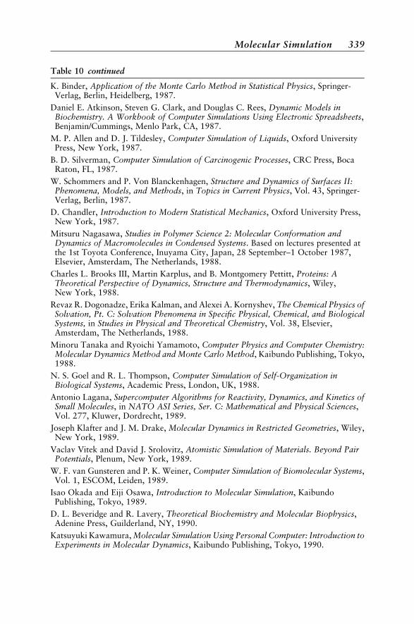
Table 10 continued

K. Binder, Application of the Monte Carlo Method in Statistical Physics, Springer-Verlag, Berlin, Heidelberg, 1987.

Daniel E. Atkinson, Steven G. Clark, and Douglas C. Rees, Dynamic Models inBiochemistry. A Workbook of Computer Simulations Using Electronic Spreadsheets,Benjamin/Cummings, Menlo Park, CA, 1987.

M. P. Allen and D. J. Tildesley, Computer Simulation of Liquids, Oxford UniversityPress, New York, 1987.

B. D. Silverman, Computer Simulation of Carcinogenic Processes, CRC Press, BocaRaton, FL, 1987.

W. Schommers and P. Von Blanckenhagen, Structure and Dynamics of Surfaces II:Phenomena, Models, and Methods, in Topics in Current Physics, Vol. 43, Springer-Verlag, Berlin, 1987.

D. Chandler, Introduction to Modern Statistical Mechanics, Oxford University Press,New York, 1987.

Mitsuru Nagasawa, Studies in Polymer Science 2: Molecular Conformation andDynamics of Macromolecules in Condensed Systems. Based on lectures presented atthe 1st Toyota Conference, Inuyama City, Japan, 28 September–1 October 1987,Elsevier, Amsterdam, The Netherlands, 1988.

Charles L. Brooks III, Martin Karplus, and B. Montgomery Pettitt, Proteins: ATheoretical Perspective of Dynamics, Structure and Thermodynamics, Wiley,New York, 1988.

Revaz R. Dogonadze, Erika Kalman, and Alexei A. Kornyshev, The Chemical Physics ofSolvation, Pt. C: Solvation Phenomena in Specific Physical, Chemical, and BiologicalSystems, in Studies in Physical and Theoretical Chemistry, Vol. 38, Elsevier,Amsterdam, The Netherlands, 1988.

Minoru Tanaka and Ryoichi Yamamoto, Computer Physics and Computer Chemistry:Molecular Dynamics Method and Monte Carlo Method, Kaibundo Publishing, Tokyo,1988.

N. S. Goel and R. L. Thompson, Computer Simulation of Self-Organization inBiological Systems, Academic Press, London, UK, 1988.

Antonio Lagana, Supercomputer Algorithms for Reactivity, Dynamics, and Kinetics ofSmall Molecules, in NATO ASI Series, Ser. C: Mathematical and Physical Sciences,Vol. 277, Kluwer, Dordrecht, 1989.

Joseph Klafter and J. M. Drake, Molecular Dynamics in Restricted Geometries, Wiley,New York, 1989.

Vaclav Vitek and David J. Srolovitz, Atomistic Simulation of Materials. Beyond PairPotentials, Plenum, New York, 1989.

W. F. van Gunsteren and P. K. Weiner, Computer Simulation of Biomolecular Systems,Vol. 1, ESCOM, Leiden, 1989.

Isao Okada and Eiji Osawa, Introduction to Molecular Simulation, KaibundoPublishing, Tokyo, 1989.

D. L. Beveridge and R. Lavery, Theoretical Biochemistry and Molecular Biophysics,Adenine Press, Guilderland, NY, 1990.

Katsuyuki Kawamura, Molecular Simulation Using Personal Computer: Introduction toExperiments in Molecular Dynamics, Kaibundo Publishing, Tokyo, 1990.

Molecular Simulation 339

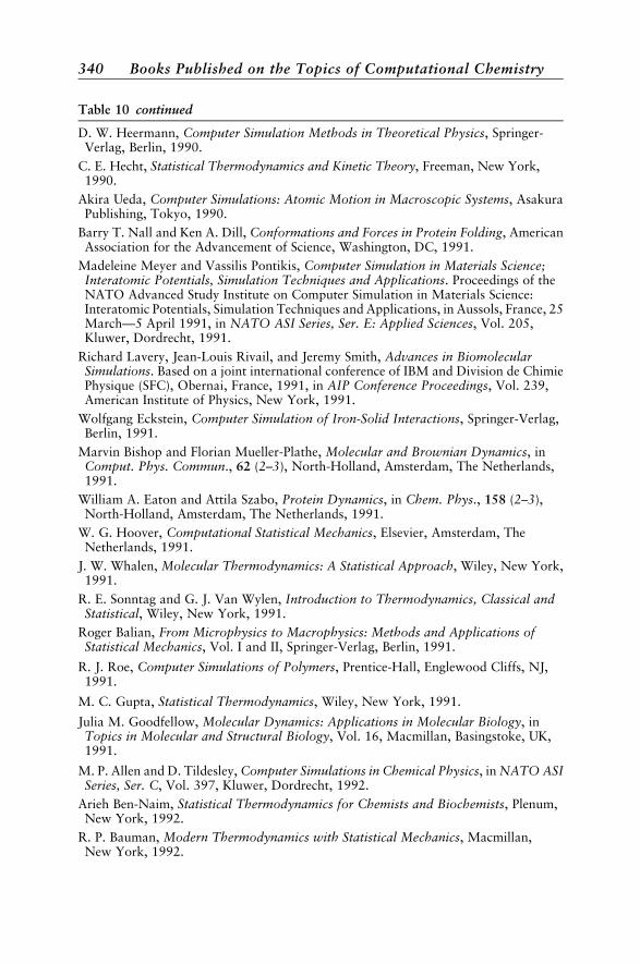
Table 10 continued

D. W. Heermann, Computer Simulation Methods in Theoretical Physics, Springer-Verlag, Berlin, 1990.

C. E. Hecht, Statistical Thermodynamics and Kinetic Theory, Freeman, New York,1990.

Akira Ueda, Computer Simulations: Atomic Motion in Macroscopic Systems, AsakuraPublishing, Tokyo, 1990.

Barry T. Nall and Ken A. Dill, Conformations and Forces in Protein Folding, AmericanAssociation for the Advancement of Science, Washington, DC, 1991.

Madeleine Meyer and Vassilis Pontikis, Computer Simulation in Materials Science;Interatomic Potentials, Simulation Techniques and Applications. Proceedings of theNATO Advanced Study Institute on Computer Simulation in Materials Science:Interatomic Potentials, Simulation Techniques and Applications, in Aussols, France, 25March—5 April 1991, in NATO ASI Series, Ser. E: Applied Sciences, Vol. 205,Kluwer, Dordrecht, 1991.

Richard Lavery, Jean-Louis Rivail, and Jeremy Smith, Advances in BiomolecularSimulations. Based on a joint international conference of IBM and Division de ChimiePhysique (SFC), Obernai, France, 1991, in AIP Conference Proceedings, Vol. 239,American Institute of Physics, New York, 1991.

Wolfgang Eckstein, Computer Simulation of Iron-Solid Interactions, Springer-Verlag,Berlin, 1991.

Marvin Bishop and Florian Mueller-Plathe, Molecular and Brownian Dynamics, inComput. Phys. Commun., 62 (2–3), North-Holland, Amsterdam, The Netherlands,1991.

William A. Eaton and Attila Szabo, Protein Dynamics, in Chem. Phys., 158 (2–3),North-Holland, Amsterdam, The Netherlands, 1991.

W. G. Hoover, Computational Statistical Mechanics, Elsevier, Amsterdam, TheNetherlands, 1991.

J. W. Whalen, Molecular Thermodynamics: A Statistical Approach, Wiley, New York,1991.

R. E. Sonntag and G. J. Van Wylen, Introduction to Thermodynamics, Classical andStatistical, Wiley, New York, 1991.

Roger Balian, From Microphysics to Macrophysics: Methods and Applications ofStatistical Mechanics, Vol. I and II, Springer-Verlag, Berlin, 1991.

R. J. Roe, Computer Simulations of Polymers, Prentice-Hall, Englewood Cliffs, NJ,1991.

M. C. Gupta, Statistical Thermodynamics, Wiley, New York, 1991.

Julia M. Goodfellow, Molecular Dynamics: Applications in Molecular Biology, inTopics in Molecular and Structural Biology, Vol. 16, Macmillan, Basingstoke, UK,1991.

M. P. Allen and D. Tildesley, Computer Simulations in Chemical Physics, in NATO ASISeries, Ser. C, Vol. 397, Kluwer, Dordrecht, 1992.

Arieh Ben-Naim, Statistical Thermodynamics for Chemists and Biochemists, Plenum,New York, 1992.

R. P. Bauman, Modern Thermodynamics with Statistical Mechanics, Macmillan,New York, 1992.

340 Books Published on the Topics of Computational Chemistry

Table 10 continued

K. Binder, The Monte Carlo Method in Condensed Matter Physics, in Top. Appl. Phys.,Vol. 71, Springer, Berlin, 1992.

Florence Baras and Daniel Walgraef, Nonequilibrium Chemical Dynamics: FromExperiment to Microscopic Simulations. NATO Advanced Research Workshop andEuropean Physical Society Liquid State Conference held at the Free University ofBrussels, Brussels, Belgium, 2–5 December 1991, in Physica A (Amsterdam), 188(1–3), North-Holland, Amsterdam, The Netherlands, 1992.

F. Yonezawa, Molecular Dynamics Simulations. Proceedings of the 13th TaniguchiSymposium, Kashikojima, Japan, November 6–9, 1990, in Springer Ser. Solid StateSci., Vol. 103, Springer, Berlin, 1992.

D. P. Landau, K. K. Mon, and H.-B. Schuettler, Computer Simulation Studies inCondensed Matter Physics IV. Proceedings of the Fourth Workshop, Athens,Georgia, February 18–22, 1991, in Springer Proc. Phys., Vol. 72, Springer, Berlin,1993.

D. P. Landau, K. K. Mon, and H.-B. Schuettler, Computer Simulation Studies inCondensed-Matter Physics V. Proceedings of the Fifth Workshop, Athens, Georgia,17–21 February 1992, in Springer Proc. Phys., Vol. 75, Springer, Berlin, 1993.

W. F. van Gunsteren, P. K. Weiner, and A. J. Wilkinson, Computer Simulation ofBiomolecular Systems, Vol. 2: Theoretical and Experimental Applications, ESCOM,Leiden, 1993.

Wayne L. Mattice and Ulrich W. Suter, Conformational Theory of Large Molecules:The Rotational Isomeric State Model in Macromolecular Systems, Wiley, New York,1994.

Katsunosuke Machida, Molecular Mechanics Method, Kodansha Co. Ltd., Tokyo,1994.

Ron Elber and Joel L. Sussman, Structure and Dynamics of Proteins, in Isr. J. Chem., 34(2), Laser Pages Publ., Jerusalem, 1994.

Sebastian Doniach, Statistical Mechanics, Protein Structure, and Protein SubstrateInteractions. Proceedings of a NATO Advanced Research Workshop on StatisticalMechanics, Protein Structure, and Protein Substrate Interactions, held June 1–5, 1993,in Cargese, Corsica, France, Plenum, New York, 1994.

Yosuke Kataoka, Computation Chemistry Series: Molecular Dynamics Method andMonte Carlo Method, Kodansha Co. Ltd., Tokyo, 1994.

Y. Hiwatari, Fundamentals and Applications of Molecular Simulation, Gordon &Breach, Yverdon, Switzerland, 1994.

Elizabeth A. Colbourn, Computer Simulation of Polymers, Longman, Harlow, UK,1994.

William L. Hase, Dynamics of Ion-Molecule Complexes, in Adv. Classical TrajectoryMethods, Vol. 2, JAI Press, Greenwich, CT, 1994.

T. A. Vilgis, Statistical Mechanics of Condensed Polymer Systems: Theory andSimulations. Based on a symposium held in Mainz, Germany, October 4–6, 1993, inMacromol. Symp., Vol. 81, Huethig and Wepf, Basel, 1994.

R. P. H. Gasser and W. G. Richards, Introduction to Statistical Thermodynamics,World Scientific, Singapore, 1995.

Claude Garrod, Statistical Mechanics and Thermodynamics—PC Version, OxfordUniversity Press, Oxford, UK, 1995.

Molecular Simulation 341

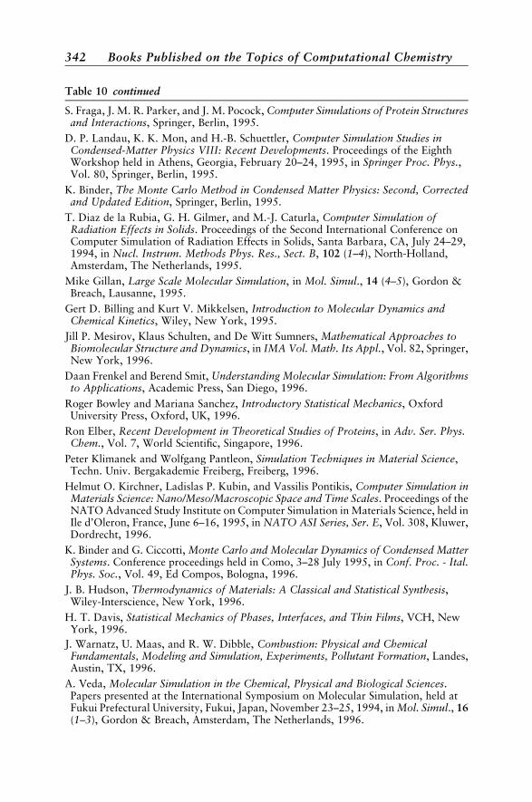
Table 10 continued

S. Fraga, J. M. R. Parker, and J. M. Pocock, Computer Simulations of Protein Structuresand Interactions, Springer, Berlin, 1995.

D. P. Landau, K. K. Mon, and H.-B. Schuettler, Computer Simulation Studies inCondensed-Matter Physics VIII: Recent Developments. Proceedings of the EighthWorkshop held in Athens, Georgia, February 20–24, 1995, in Springer Proc. Phys.,Vol. 80, Springer, Berlin, 1995.

K. Binder, The Monte Carlo Method in Condensed Matter Physics: Second, Correctedand Updated Edition, Springer, Berlin, 1995.

T. Diaz de la Rubia, G. H. Gilmer, and M.-J. Caturla, Computer Simulation ofRadiation Effects in Solids. Proceedings of the Second International Conference onComputer Simulation of Radiation Effects in Solids, Santa Barbara, CA, July 24–29,1994, in Nucl. Instrum. Methods Phys. Res., Sect. B, 102 (1–4), North-Holland,Amsterdam, The Netherlands, 1995.

Mike Gillan, Large Scale Molecular Simulation, in Mol. Simul., 14 (4–5), Gordon &Breach, Lausanne, 1995.

Gert D. Billing and Kurt V. Mikkelsen, Introduction to Molecular Dynamics andChemical Kinetics, Wiley, New York, 1995.

Jill P. Mesirov, Klaus Schulten, and De Witt Sumners, Mathematical Approaches toBiomolecular Structure and Dynamics, in IMA Vol. Math. Its Appl., Vol. 82, Springer,New York, 1996.

Daan Frenkel and Berend Smit, Understanding Molecular Simulation: From Algorithmsto Applications, Academic Press, San Diego, 1996.

Roger Bowley and Mariana Sanchez, Introductory Statistical Mechanics, OxfordUniversity Press, Oxford, UK, 1996.

Ron Elber, Recent Development in Theoretical Studies of Proteins, in Adv. Ser. Phys.Chem., Vol. 7, World Scientific, Singapore, 1996.

Peter Klimanek and Wolfgang Pantleon, Simulation Techniques in Material Science,Techn. Univ. Bergakademie Freiberg, Freiberg, 1996.

Helmut O. Kirchner, Ladislas P. Kubin, and Vassilis Pontikis, Computer Simulation inMaterials Science: Nano/Meso/Macroscopic Space and Time Scales. Proceedings of theNATO Advanced Study Institute on Computer Simulation in Materials Science, held inIle d’Oleron, France, June 6–16, 1995, in NATO ASI Series, Ser. E, Vol. 308, Kluwer,Dordrecht, 1996.

K. Binder and G. Ciccotti, Monte Carlo and Molecular Dynamics of Condensed MatterSystems. Conference proceedings held in Como, 3–28 July 1995, in Conf. Proc. - Ital.Phys. Soc., Vol. 49, Ed Compos, Bologna, 1996.

J. B. Hudson, Thermodynamics of Materials: A Classical and Statistical Synthesis,Wiley-Interscience, New York, 1996.

H. T. Davis, Statistical Mechanics of Phases, Interfaces, and Thin Films, VCH, NewYork, 1996.

J. Warnatz, U. Maas, and R. W. Dibble, Combustion: Physical and ChemicalFundamentals, Modeling and Simulation, Experiments, Pollutant Formation, Landes,Austin, TX, 1996.

A. Veda, Molecular Simulation in the Chemical, Physical and Biological Sciences.Papers presented at the International Symposium on Molecular Simulation, held atFukui Prefectural University, Fukui, Japan, November 23–25, 1994, in Mol. Simul., 16(1–3), Gordon & Breach, Amsterdam, The Netherlands, 1996.

342 Books Published on the Topics of Computational Chemistry

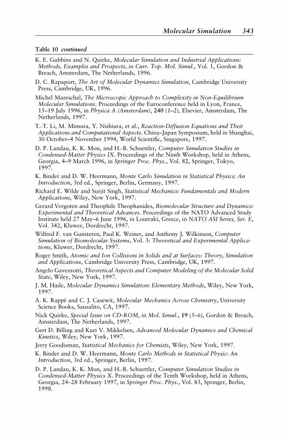
Table 10 continued

K. E. Gubbins and N. Quirke, Molecular Simulation and Industrial Applications:Methods, Examples and Prospects, in Curr. Top. Mol. Simul., Vol. 1, Gordon &Breach, Amsterdam, The Netherlands, 1996.

D. C. Rapaport, The Art of Molecular Dynamics Simulation, Cambridge UniversityPress, Cambridge, UK, 1996.

Michel Mareschal, The Microscopic Approach to Complexity in Non-EquilibriumMolecular Simulations. Proceedings of the Euroconference held in Lyon, France,15–19 July 1996, in Physica A (Amsterdam), 240 (1–2), Elsevier, Amsterdam, TheNetherlands, 1997.

T.-T. Li, M. Mimura, Y. Nishiura, et al., Reaction-Diffusion Equations and TheirApplications and Computational Aspects. China–Japan Symposium, held in Shanghai,30 October–4 November 1994, World Scientific, Singapore, 1997.

D. P. Landau, K. K. Mon, and H.-B. Schuettler, Computer Simulation Studies inCondensed-Matter Physics IX. Proceedings of the Ninth Workshop, held in Athens,Georgia, 4–9 March 1996, in Springer Proc. Phys., Vol. 82, Springer, Tokyo,1997.

K. Binder and D. W. Heermann, Monte Carlo Simulation in Statistical Physics: AnIntroduction, 3rd ed., Springer, Berlin, Germany, 1997.

Richard E. Wilde and Surjit Singh, Statistical Mechanics: Fundamentals and ModernApplications, Wiley, New York, 1997.

Gerard Vergoten and Theophile Theophanides, Biomolecular Structure and Dynamics:Experimental and Theoretical Advances. Proceedings of the NATO Advanced StudyInstitute held 27 May–6 June 1996, in Loutraki, Greece, in NATO ASI Series, Ser. E,Vol. 342, Kluwer, Dordrecht, 1997.

Wilfred F. van Gunsteren, Paul K. Weiner, and Anthony J. Wilkinson, ComputerSimulation of Biomolecular Systems, Vol. 3: Theoretical and Experimental Applica-tions, Kluwer, Dordrecht, 1997.

Roger Smith, Atomic and Ion Collisions in Solids and at Surfaces: Theory, Simulationand Applications, Cambridge University Press, Cambridge, UK, 1997.

Angelo Gavezzotti, Theoretical Aspects and Computer Modeling of the Molecular SolidState, Wiley, New York, 1997.

J. M. Haile, Molecular Dynamics Simulation: Elementary Methods, Wiley, New York,1997.

A. K. Rappe and C. J. Casewit, Molecular Mechanics Across Chemistry, UniversityScience Books, Sausalito, CA, 1997.

Nick Quirke, Special Issue on CD-ROM, in Mol. Simul., 19 (5–6), Gordon & Breach,Amsterdam, The Netherlands, 1997.

Gert D. Billing and Kurt V. Mikkelsen, Advanced Molecular Dynamics and ChemicalKinetics, Wiley, New York, 1997.

Jerry Goodisman, Statistical Mechanics for Chemists, Wiley, New York, 1997.

K. Binder and D. W. Heermann, Monte Carlo Methods in Statistical Physic: AnIntroduction, 3rd ed., Springer, Berlin, 1997.

D. P. Landau, K. K. Mon, and H.-B. Schuettler, Computer Simulation Studies inCondensed-Matter Physics X. Proceedings of the Tenth Workshop, held in Athens,Georgia, 24–28 February 1997, in Springer Proc. Phys., Vol. 83, Springer, Berlin,1998.

Molecular Simulation 343

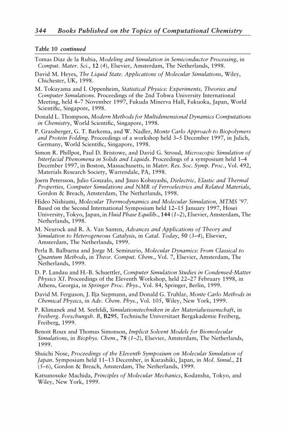
Table 10 continued

Tomas Diaz de la Rubia, Modeling and Simulation in Semiconductor Processing, inComput. Mater. Sci., 12 (4), Elsevier, Amsterdam, The Netherlands, 1998.

David M. Heyes, The Liquid State. Applications of Molecular Simulations, Wiley,Chichester, UK, 1998.

M. Tokuyama and I. Oppenheim, Statistical Physics: Experiments, Theories andComputer Simulations. Proceedings of the 2nd Tohwa University InternationalMeeting, held 4–7 November 1997, Fukuda Minerva Hall, Fukuoka, Japan, WorldScientific, Singapore, 1998.

Donald L. Thompson, Modern Methods for Multidimensional Dynamics Computationsin Chemistry, World Scientific, Singapore, 1998.

P. Grassberger, G. T. Barkema, and W. Nadler, Monte Carlo Approach to Biopolymersand Protein Folding. Proceedings of a workshop held 3–5 December 1997, in Julich,Germany, World Scientific, Singapore, 1998.

Simon R. Phillpot, Paul D. Bristowe, and David G. Stroud, Microscopic Simulation ofInterfacial Phenomena in Solids and Liquids. Proceedings of a symposium held 1–4December 1997, in Boston, Massachusetts, in Mater. Res. Soc. Symp. Proc., Vol. 492,Materials Research Society, Warrendale, PA, 1998.

Joern Petersson, Julio Gonzalo, and Jinzo Kobayashi, Dielectric, Elastic and ThermalProperties, Computer Simulations and NMR of Ferroelectrics and Related Materials,Gordon & Breach, Amsterdam, The Netherlands, 1998.

Hideo Nishiumi, Molecular Thermodynamics and Molecular Simulation, MTMS ’97.Based on the Second International Symposium held 12–15 January 1997, HoseiUniversity, Tokyo, Japan, in Fluid Phase Equilib., 144 (1–2), Elsevier, Amsterdam, TheNetherlands, 1998.

M. Neurock and R. A. Van Santen, Advances and Applications of Theory andSimulation to Heterogeneous Catalysis, in Catal. Today, 50 (3–4), Elsevier,Amsterdam, The Netherlands, 1999.

Perla B. Balbuena and Jorge M. Seminario, Molecular Dynamics: From Classical toQuantum Methods, in Theor. Comput. Chem., Vol. 7, Elsevier, Amsterdam, TheNetherlands, 1999.

D. P. Landau and H.-B. Schuettler, Computer Simulation Studies in Condensed-MatterPhysics XI. Proceedings of the Eleventh Workshop, held 22–27 February 1998, inAthens, Georgia, in Springer Proc. Phys., Vol. 84, Springer, Berlin, 1999.

David M. Ferguson, J. Ilja Siepmann, and Donald G. Truhlar, Monte Carlo Methods inChemical Physics, in Adv. Chem. Phys., Vol. 105, Wiley, New York, 1999.

P. Klimanek and M. Seefeldi, Simulationstechniken in der Materialwissenschaft, inFreiberg. Forschungsh. B, B295, Technische Universitaet Bergakademie Freiberg,Freiberg, 1999.

Benoit Roux and Thomas Simonson, Implicit Solvent Models for BiomolecularSimulations, in Biophys. Chem., 78 (1–2), Elsevier, Amsterdam, The Netherlands,1999.

Shuichi Nose, Proceedings of the Eleventh Symposium on Molecular Simulation ofJapan. Symposium held 11–13 December, in Kurashiki, Japan, in Mol. Simul., 21(5–6), Gordon & Breach, Amsterdam, The Netherlands, 1999.

Katsunosuke Machida, Principles of Molecular Mechanics, Kodansha, Tokyo, andWiley, New York, 1999.

344 Books Published on the Topics of Computational Chemistry

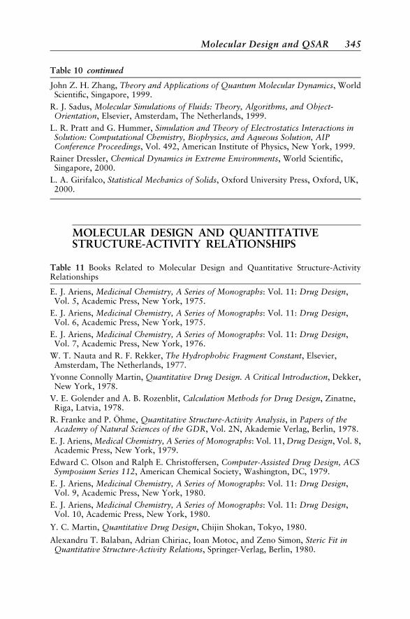
Table 10 continued

John Z. H. Zhang, Theory and Applications of Quantum Molecular Dynamics, WorldScientific, Singapore, 1999.

R. J. Sadus, Molecular Simulations of Fluids: Theory, Algorithms, and Object-Orientation, Elsevier, Amsterdam, The Netherlands, 1999.

L. R. Pratt and G. Hummer, Simulation and Theory of Electrostatics Interactions inSolution: Computational Chemistry, Biophysics, and Aqueous Solution, AIPConference Proceedings, Vol. 492, American Institute of Physics, New York, 1999.

Rainer Dressler, Chemical Dynamics in Extreme Environments, World Scientific,Singapore, 2000.

L. A. Girifalco, Statistical Mechanics of Solids, Oxford University Press, Oxford, UK,2000.

MOLECULAR DESIGN AND QUANTITATIVESTRUCTURE-ACTIVITY RELATIONSHIPS

Table 11 Books Related to Molecular Design and Quantitative Structure-ActivityRelationships

E. J. Ariens, Medicinal Chemistry, A Series of Monographs: Vol. 11: Drug Design,Vol. 5, Academic Press, New York, 1975.

E. J. Ariens, Medicinal Chemistry, A Series of Monographs: Vol. 11: Drug Design,Vol. 6, Academic Press, New York, 1975.

E. J. Ariens, Medicinal Chemistry, A Series of Monographs: Vol. 11: Drug Design,Vol. 7, Academic Press, New York, 1976.

W. T. Nauta and R. F. Rekker, The Hydrophobic Fragment Constant, Elsevier,Amsterdam, The Netherlands, 1977.

Yvonne Connolly Martin, Quantitative Drug Design. A Critical Introduction, Dekker,New York, 1978.

V. E. Golender and A. B. Rozenblit, Calculation Methods for Drug Design, Zinatne,Riga, Latvia, 1978.

R. Franke and P. Ohme, Quantitative Structure-Activity Analysis, in Papers of theAcademy of Natural Sciences of the GDR, Vol. 2N, Akademie Verlag, Berlin, 1978.

E. J. Ariens, Medical Chemistry, A Series of Monographs: Vol. 11, Drug Design, Vol. 8,Academic Press, New York, 1979.

Edward C. Olson and Ralph E. Christoffersen, Computer-Assisted Drug Design, ACSSymposium Series 112, American Chemical Society, Washington, DC, 1979.

E. J. Ariens, Medicinal Chemistry, A Series of Monographs: Vol. 11: Drug Design,Vol. 9, Academic Press, New York, 1980.

E. J. Ariens, Medicinal Chemistry, A Series of Monographs: Vol. 11: Drug Design,Vol. 10, Academic Press, New York, 1980.

Y. C. Martin, Quantitative Drug Design, Chijin Shokan, Tokyo, 1980.

Alexandru T. Balaban, Adrian Chiriac, Ioan Motoc, and Zeno Simon, Steric Fit inQuantitative Structure-Activity Relations, Springer-Verlag, Berlin, 1980.

Molecular Design and QSAR 345

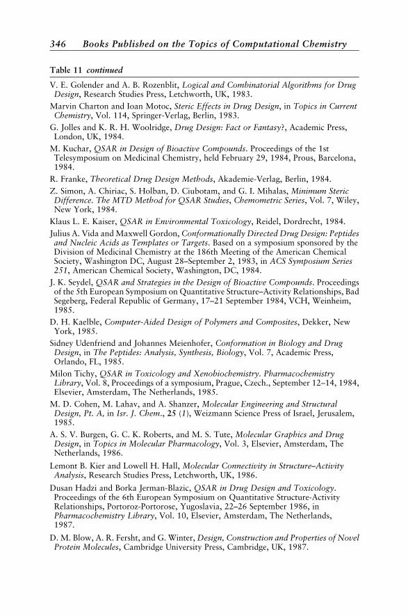
Table 11 continued

V. E. Golender and A. B. Rozenblit, Logical and Combinatorial Algorithms for DrugDesign, Research Studies Press, Letchworth, UK, 1983.

Marvin Charton and Ioan Motoc, Steric Effects in Drug Design, in Topics in CurrentChemistry, Vol. 114, Springer-Verlag, Berlin, 1983.

G. Jolles and K. R. H. Woolridge, Drug Design: Fact or Fantasy?, Academic Press,London, UK, 1984.

M. Kuchar, QSAR in Design of Bioactive Compounds. Proceedings of the 1stTelesymposium on Medicinal Chemistry, held February 29, 1984, Prous, Barcelona,1984.

R. Franke, Theoretical Drug Design Methods, Akademie-Verlag, Berlin, 1984.

Z. Simon, A. Chiriac, S. Holban, D. Ciubotam, and G. I. Mihalas, Minimum StericDifference. The MTD Method for QSAR Studies, Chemometric Series, Vol. 7, Wiley,New York, 1984.

Klaus L. E. Kaiser, QSAR in Environmental Toxicology, Reidel, Dordrecht, 1984.

Julius A. Vida and Maxwell Gordon, Conformationally Directed Drug Design: Peptidesand Nucleic Acids as Templates or Targets. Based on a symposium sponsored by theDivision of Medicinal Chemistry at the 186th Meeting of the American ChemicalSociety, Washington DC, August 28–September 2, 1983, in ACS Symposium Series251, American Chemical Society, Washington, DC, 1984.

J. K. Seydel, QSAR and Strategies in the Design of Bioactive Compounds. Proceedingsof the 5th European Symposium on Quantitative Structure–Activity Relationships, BadSegeberg, Federal Republic of Germany, 17–21 September 1984, VCH, Weinheim,1985.

D. H. Kaelble, Computer-Aided Design of Polymers and Composites, Dekker, NewYork, 1985.

Sidney Udenfriend and Johannes Meienhofer, Conformation in Biology and DrugDesign, in The Peptides: Analysis, Synthesis, Biology, Vol. 7, Academic Press,Orlando, FL, 1985.

Milon Tichy, QSAR in Toxicology and Xenobiochemistry. PharmacochemistryLibrary, Vol. 8, Proceedings of a symposium, Prague, Czech., September 12–14, 1984,Elsevier, Amsterdam, The Netherlands, 1985.

M. D. Cohen, M. Lahav, and A. Shanzer, Molecular Engineering and StructuralDesign, Pt. A, in Isr. J. Chem., 25 (1), Weizmann Science Press of Israel, Jerusalem,1985.

A. S. V. Burgen, G. C. K. Roberts, and M. S. Tute, Molecular Graphics and DrugDesign, in Topics in Molecular Pharmacology, Vol. 3, Elsevier, Amsterdam, TheNetherlands, 1986.

Lemont B. Kier and Lowell H. Hall, Molecular Connectivity in Structure–ActivityAnalysis, Research Studies Press, Letchworth, UK, 1986.

Dusan Hadzi and Borka Jerman-Blazic, QSAR in Drug Design and Toxicology.Proceedings of the 6th European Symposium on Quantitative Structure-ActivityRelationships, Portoroz-Portorose, Yugoslavia, 22–26 September 1986, inPharmacochemistry Library, Vol. 10, Elsevier, Amsterdam, The Netherlands,1987.

D. M. Blow, A. R. Fersht, and G. Winter, Design, Construction and Properties of NovelProtein Molecules, Cambridge University Press, Cambridge, UK, 1987.

346 Books Published on the Topics of Computational Chemistry

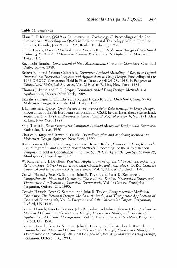
Table 11 continued

Klaus L. E. Kaiser, QSAR in Environmental Toxicology II. Proceedings of the 2ndInternational Workshop on QSAR in Environmental Toxicology held in Hamilton,Ontario, Canada, June 9–13, 1986, Reidel, Dordrecht, 1987.

Sumio Tokita, Masaru Matsuoka, and Yoshiya Kogo, Molecular Design of FunctionalColoring Matter: PPP Molecular Orbital Method and Its Application, Maruzen,Tokyo, 1989.

Kazutoshi Tanabe, Development of New Materials and Computer Chemistry, ChemicalDaily, Tokyo, 1989.

Robert Rein and Amram Golombek, Computer-Assisted Modeling of Receptor-LigandInteractions: Theoretical Aspects and Applications to Drug Design. Proceedings of the1988 OHOLO Conference Held in Eilat, Israel, April 24–28, 1988, in Progress inClinical and Biological Research, Vol. 289, Alan R. Liss, New York, 1989.

Thomas J. Perun and C. L. Propst, Computer-Aided Drug Design. Methods andApplications, Dekker, New York, 1989.

Kizashi Yamaguchi, Shinichi Yamabe, and Kazuo Kitaura, Quantum Chemistry forMolecular Design, Kodansha Ltd., Tokyo, 1989.

J. L. Fauchere, QSAR: Quantitative Structure–Activity Relationships in Drug Design.Proceedings of the 7th European Symposium on QSAR held in Interlaken, Switzerland,September 5–9, 1988, in Progress in Clinical and Biological Research, Vol. 291, AlanR. Liss, New York, 1989.

Shuji Tomoda, Basic Systems for Computer Assisted Molecular Design with Exercises,Kodansha, Tokyo, 1990.

Charles E. Bugg and Steven E. Ealick, Crystallographic and Modeling Methods inMolecular Design, Springer, New York, 1990.

Birthe Jensen, Flemming S. Jørgensen, and Helmer Kofod, Frontiers in Drug Research:Crystallographic and Computational Methods. Proceedings of the Alfred BenzonSymposium held in Copenhagen, June 11–15, 1989, in Alfred Benzon Symposium 28,Munksgaard, Copenhagen, 1990.

W. Karcher and J. Devillers, Practical Applications of Quantitative Structure–ActivityRelationships (QSAR) in Environmental Chemistry and Toxicology. EURO Courses:Chemical and Environmental Science Series, Vol. 1, Kluwer, Dordrecht, 1990.

Corwin Hansch, Peter G. Sammes, John B. Taylor, and Peter D. Kennewell,Comprehensive Medicinal Chemistry. The Rational Design, Mechanistic Study, andTherapeutic Application of Chemical Compounds, Vol. 1: General Principles,Pergamon, Oxford, UK, 1990.

Corwin Hansch, Peter G. Sammes, and John B. Taylor, Comprehensive MedicinalChemistry. The Rational Design, Mechanistic Study, and Therapeutic Application ofChemical Compounds, Vol. 2: Enzymes and Other Molecular Targets, Pergamon,Oxford, UK, 1990.

Corwin Hansch, Peter G. Sammes, John B. Taylor, and John C. Emmett, ComprehensiveMedicinal Chemistry. The Rational Design, Mechanistic Study, and TherapeuticApplication of Chemical Compounds, Vol. 3: Membranes and Receptors, Pergamon,Oxford, UK, 1990.

Corwin Hansch, Peter G. Sammes, John B. Taylor, and Christopher A. Ramsden,Comprehensive Medicinal Chemistry. The Rational Design, Mechanistic Study, andTherapeutic Application of Chemical Compounds, Vol. 4: Quantitative Drug Design,Pergamon, Oxford, UK, 1990.

Molecular Design and QSAR 347

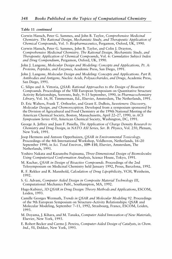
Table 11 continued

Corwin Hansch, Peter G. Sammes, and John B. Taylor, Comprehensive MedicinalChemistry. The Rational Design, Mechanistic Study, and Therapeutic Application ofChemical Compounds, Vol. 5: Biopharmaceutics, Pergamon, Oxford, UK, 1990.

Corwin Hansch, Peter G. Sammes, John B. Taylor, and Colin J. Drayton,Comprehensive Medicinal Chemistry. The Rational Design, Mechanistic Study, andTherapeutic Application of Chemical Compounds, Vol. 6: Cumulative Subject Indexand Drug Compendium, Pergamon, Oxford, UK, 1990.

John J. Langone, Molecular Design and Modeling: Concepts and Applications, Pt. A:Proteins, Peptides, and Enzymes, Academic Press, San Diego, 1991.

John J. Langone, Molecular Design and Modeling: Concepts and Applications. Part B.Antibodies and Antigens, Nucleic Acids, Polysaccharides, and Drugs, Academic Press,San Diego, 1991.

C. Silipo and A. Vittoria, QSAR: Rational Approaches to the Design of BioactiveCompounds. Proceedings of the VIII European Symposium on Quantitative StructureActivity Relationships, Sorrento, Italy, 9–13 September, 1990, in PharmacochemistryLibrary, Vol. 16, H. Timmerman, Ed., Elsevier, Amsterdam, The Netherlands, 1991.

D. Eric Walters, Frank T. Orthoefer, and Grant E. DuBois, Sweeteners: Discovery,Molecular Design, and Chemoreception. Developed from a symposium sponsored bythe Division of Agricultural and Food Chemistry at the 199th National Meeting of theAmerican Chemical Society, Boston, Massachusetts, April 22–27, 1990, in ACSSymposium Series 450, American Chemical Society, Washington, DC, 1991.

George A. Jeffrey and Juan F. Piniella, The Application of Charge Density Research toChemistry and Drug Design, in NATO ASI Series, Ser. B: Physics, Vol. 250, Plenum,New York, 1991.

Joop Hermens and Antoon Opperhuizen, QSAR in Environmental Toxicology.Proceedings of the 4th International Workshop, Veldhoven, Netherlands, 16–20September 1990, in Sci. Total Environ., 109–110, Elsevier, Amsterdam, TheNetherlands, 1991.

Yoshiro Nakata and Kazunobu Fujinuma, Three-Dimensional Design of BiomoleculesUsing Computerized Conformation Analysis, Science House, Tokyo, 1991.

M. Kuchar, QSAR in Design of Bioactive Compounds. Proceedings of the 2ndTelesymposium on Medicinal Chemistry held January 1992, Prous, Barcelona, 1992.

R. F. Rekker and R. Mannhold, Calculation of Drug Lipophilicity, VCH, Weinheim,1992.

S. G. Advani, Computer Aided Design in Composite Material Technology III,Computational Mechanics Publ., Southampton, MA, 1992.

Hugo Kubinyi, 3D QSAR in Drug Design: Theory Methods and Applications, ESCOM,Leiden, 1993.

Camille Georges Wermuth, Trends in QSAR and Molecular Modeling 92. Proceedingsof the 9th European Symposium on Structure–Activity Relationships: QSAR andMolecular Modeling, September 7–11, 1992, Strasbourg, France, ESCOM, Leiden,1993.

M. Doyama, J. Kihara, and M. Tanaka, Computer Aided Innovation of New Materials,Elsevier, New York, 1993.

E. Robert Becker and Carmo J. Pereira, Computer-Aided Design of Catalysts, in Chem.Ind., 51, Dekker, New York, 1993.

348 Books Published on the Topics of Computational Chemistry

Table 11 continued

Hugo Kubinyi, QSAR: Hansch Analysis and Related Approaches, VCH, Weinheim,1994.

J. G. Vinter and Mark Gardner, Molecular Modeling and Drug Design, CRC, BocaRaton, FL, 1994.

Kazuyuki Hirao and Katsuyuki Kawamura, Material Design Using Personal Computer:Programs of Molecular Dynamics with a Floppy Disk, Shokabo, Tokyo, 1994.

Toshio Fujita, QSAR and Drug Design: New Developments and Applications, inPharmacochemistry Library, Vol. 23, Elsevier, Amsterdam, The Netherlands, 1995.

W. J. Zeller, M. D’Incalci, and D. R. Newell, Novel Approaches in Anticancer DrugDesign: Molecular Modeling – New Treatment Strategies. International Symposium onNovel Approaches in Cancer Therapy, Heidelberg, December 1–4, 1993, in Contrib.Oncol., Vol. 49, Karger, Basel, 1995.

Walter Karcher, Quantitative Structure–Activity Relationships (QSAR) in Environ-mental Sciences. Based on the 6th International Workshop held in Belgirate, Italy,13–17 September 1994, in SAR QSAR Environ. Res., 3 (3), Gordon & Breach,Lausanne, 1995.

Walter Karcher, Quantitative Structure-Activity Relationships (QSAR) in Environ-mental Sciences. Based on the 6th International Workshop held in Belgirate, Italy,13–17 September 1994, in SAR QSAR Environ. Res., 4 (1), Gordon & Breach,Amsterdam, The Netherlands, 1995.

Han van de Waterbeemd, Chemometric Methods in Molecular Design, in MethodsPrinc. Med. Chem., Vol. 2, VCH, Weinheim, 1995.

P. M. Dean, G. Jolles, and C. G. Newton, New Perspectives in Drug Design, AcademicPress, London, UK, 1995.

P. M. Dean, Molecular Similarity in Drug Design, Blackie, Glasgow, UK, 1995.

E. C. Herrmann and R. Franke, Computer-Aided Drug Design in Industrial Research.The Ernst Schering Research Foundation 15th Workshop in Berlin, October 19–21,1994, in Ernst Schering Res. Found. Workshop, Vol. 15, Springer, Berlin, 1995.

Charles H. Reynolds, M. Katharine Holloway, and Harold K. Cox, Computer-AidedMolecular Design: Applications in Agrochemicals, Materials, and Pharmaceuticals.Developed from a symposium sponsored by the Division of Computers in Chemistryand the Division of Agrochemicals at the 207th National Meeting of the ACS, SanDiego, CA, March 13–17, 1994, in ACS Symposium Series 589, American ChemicalSociety, Washington, DC, 1995.

Charles H. Reynolds, M. Katharine Holloway, and Harold K. Cox, Computer-AidedMolecular Design: Applications in Agrochemicals, Materials, and Pharmaceuticals,Tec and Doc - Lavoisier, Paris, 1995.

Corwin Hansch and Albert Leo, Exploring QSAR. Fundamentals and Applications inChemistry and Biology, American Chemical Society, Washington, DC, 1995.

Corwin Hansch, Albert Leo, and David Hoekman, Exploring QSAR. Hydrophobic,Electronic, and Steric Constants, American Chemical Society, Washington, DC, 1995.

Corwin Hansch and Toshio Fujita, Classical and Three-Dimensional QSAR inAgrochemistry. Developed from a symposium sponsored by the Division ofAgrochemicals at the 208th National Meeting of the American Chemical Society,Washington, DC, August 21–25, 1994, in ACS Symposium Series 606, AmericanChemical Society, Washington, DC, 1995.

Molecular Design and QSAR 349

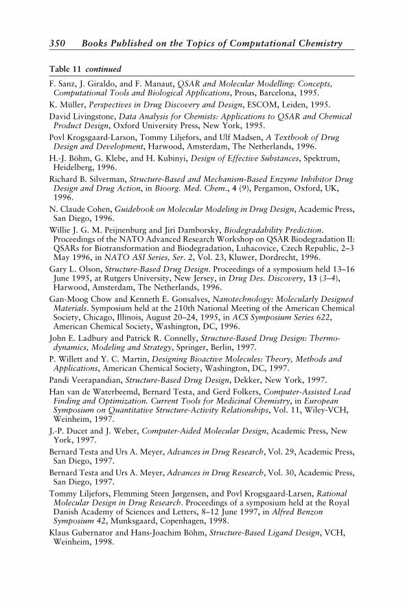
Table 11 continued

F. Sanz, J. Giraldo, and F. Manaut, QSAR and Molecular Modelling: Concepts,Computational Tools and Biological Applications, Prous, Barcelona, 1995.

K. Muller, Perspectives in Drug Discovery and Design, ESCOM, Leiden, 1995.

David Livingstone, Data Analysis for Chemists: Applications to QSAR and ChemicalProduct Design, Oxford University Press, New York, 1995.

Povl Krogsgaard-Larson, Tommy Liljefors, and Ulf Madsen, A Textbook of DrugDesign and Development, Harwood, Amsterdam, The Netherlands, 1996.

H.-J. Bohm, G. Klebe, and H. Kubinyi, Design of Effective Substances, Spektrum,Heidelberg, 1996.

Richard B. Silverman, Structure-Based and Mechanism-Based Enzyme Inhibitor DrugDesign and Drug Action, in Bioorg. Med. Chem., 4 (9), Pergamon, Oxford, UK,1996.

N. Claude Cohen, Guidebook on Molecular Modeling in Drug Design, Academic Press,San Diego, 1996.

Willie J. G. M. Peijnenburg and Jiri Damborsky, Biodegradability Prediction.Proceedings of the NATO Advanced Research Workshop on QSAR Biodegradation II:QSARs for Biotransformation and Biodegradation, Luhacovice, Czech Republic, 2–3May 1996, in NATO ASI Series, Ser. 2, Vol. 23, Kluwer, Dordrecht, 1996.

Gary L. Olson, Structure-Based Drug Design. Proceedings of a symposium held 13–16June 1995, at Rutgers University, New Jersey, in Drug Des. Discovery, 13 (3–4),Harwood, Amsterdam, The Netherlands, 1996.

Gan-Moog Chow and Kenneth E. Gonsalves, Nanotechnology: Molecularly DesignedMaterials. Symposium held at the 210th National Meeting of the American ChemicalSociety, Chicago, Illinois, August 20–24, 1995, in ACS Symposium Series 622,American Chemical Society, Washington, DC, 1996.

John E. Ladbury and Patrick R. Connelly, Structure-Based Drug Design: Thermo-dynamics, Modeling and Strategy, Springer, Berlin, 1997.

P. Willett and Y. C. Martin, Designing Bioactive Molecules: Theory, Methods andApplications, American Chemical Society, Washington, DC, 1997.

Pandi Veerapandian, Structure-Based Drug Design, Dekker, New York, 1997.

Han van de Waterbeemd, Bernard Testa, and Gerd Folkers, Computer-Assisted LeadFinding and Optimization. Current Tools for Medicinal Chemistry, in EuropeanSymposium on Quantitative Structure-Activity Relationships, Vol. 11, Wiley-VCH,Weinheim, 1997.

J.-P. Ducet and J. Weber, Computer-Aided Molecular Design, Academic Press, NewYork, 1997.

Bernard Testa and Urs A. Meyer, Advances in Drug Research, Vol. 29, Academic Press,San Diego, 1997.

Bernard Testa and Urs A. Meyer, Advances in Drug Research, Vol. 30, Academic Press,San Diego, 1997.

Tommy Liljefors, Flemming Steen Jørgensen, and Povl Krogsgaard-Larsen, RationalMolecular Design in Drug Research. Proceedings of a symposium held at the RoyalDanish Academy of Sciences and Letters, 8–12 June 1997, in Alfred BenzonSymposium 42, Munksgaard, Copenhagen, 1998.

Klaus Gubernator and Hans-Joachim Bohm, Structure-Based Ligand Design, VCH,Weinheim, 1998.

350 Books Published on the Topics of Computational Chemistry

Table 11 continued

Anthony K. Cheetham, Ulrich W. Suter, and Erich Wimmer, Multiscale MaterialsPrediction: Fundamentals and Industrial Applications. Proceedings of a workshop held14–16 September 1997, at MIT, in J. Comput.-Aided Mater. Des., 4 (3), Kluwer,Dordrecht, 1998.

Anonymous, Organic Solids Based on p Electron Systems: Molecular Design, ElectronicProperties (Charge and Spin) and Applications, Gakkai Shuppan Center, Tokyo, 1998.

Penelope W. Codding, Structure-Based Drug Design: Experimental and ComputationalApproaches, in NATO ASI Series, Ser. E, Vol. 352, Kluwer, Dordrecht, 1998.

Yvonne Connolly Martin and Peter Willett, Designing Bioactive Molecules: Three-Dimensional Techniques and Applications, American Chemical Society, Washington,DC, 1998.

James Devillers, Comparative QSAR, Taylor and Francis, Washington, DC, 1998.

Martin Reinhard and Axel Drefahl, Handbook for Estimating PhysiochemicalProperties of Organic Compounds, Wiley, New York, 1998.

Jure Zupan and Johann Gasteiger, Neural Networks in Chemistry and Drug Design: AnIntroduction, 2nd ed., Wiley, New York, 1999.

Lemont B. Kier and Lowell H. Hall, Molecular Structure Description: The Electro-topological State, Academic Press, San Diego, 1999.

Marvin Charton and Barbara I. Charton, Advances in Quantitative Structure–PropertyRelationships. Vol. 2, JAI Press, Stamford, CT, 1999.

Gyorgy Keseru and Istvan Kolossvary, Molecular Mechanics and ConformationalAnalysis in Drug Design, Blackwell Science, Oxford, UK, 1999.

Osman F. Guner, Pharmacophore Perception, Development, and Use in Drug Design,International University Line, La Jolla, CA, 1999.

Donald G. Truhlar, W. Jeffrey Howe, Anthony J. Hopfinger, Jeff Blaney, and Richard A.Dammkoehler, Rational Drug Design, IMA Vol. Math. Its Appl., Vol. 108, Springer,New York, 1999.

Alexander Pechenik, Rajiv Kalia, and Priya Vashishta, Computer-Aided Design ofHigh-Temperature Materials, Oxford University Press, Oxford, UK, 1999.

Abby L. Parrill and M. Rami Reddy, Rational Drug Design: Novel Methodology andPractical Applications, ACS Symposium Series 719, American Chemical Society,Washington, DC, 1999.

James Devillers and Alexandru T. Balaban, Topological Indices and Related Descriptorsin QSAR and QSPR, Gordon & Breach, Amsterdam, The Netherlands, 1999.

John M. Fraser, Ruth Pachter, Steve Trohalaki, and Kevin T. Geiss, ComputationalMethods in Toxicology. Proceedings of an international workshop held 20–22 April1998, in Dayton, OH, in SAR QSAR Environ. Res., 10 (2–3), 1999.

P. G. DeBeneditti, Theoretical Approaches to Quantitative Pharmacophore Modeling—Biological Activity Relationships, Elsevier, Amsterdam, The Netherlands, 1999.

David E. Clark, Evolutionary Algorithms in Molecular Design, in Methods andPrinciples in Medicinal Chemistry, Vol. 8, R. Mannhold, H. Kubinyi, andH. Timmerman, Eds., Wiley-VCH, Weinheim, 2000.

Klaus Gundertofte and Flemming Jørgensen, Molecular Modeling and Prediction ofBioactivity, Proceedings of the 12th European Symposium on Quantitative Structure–Activity Relationships held 23–28 August 1998, in Copenhagen, Kluwer Academic/Plenum Publishers, New York, 2000.

Molecular Design and QSAR 351

Table 11 continued

Yvonne C. Martin, Hydrophobicity and Solvation in Drug Design, Part III, in Perspect.Drug Discovery Des., 19, 2000.

R. Carbo, Molecular Quantum Similarity in QSAR and Drug Design, Springer-Verlag,New York, 2000.

Hans-Joachim Bohm and Gisbert Schneider, Virtual Screening for Bioactive Molecules,Wiley, New York, 2000.

Mati Karelson, Molecular Descriptors in QSAR/QSPR, Wiley, New York, 2000.

GRAPH THEORY IN CHEMISTRY

Table 12 Books on Graph Theory in Chemistry

Frantisek Hrncirik, Properties of Hydrocarbons C1–C8 Determined by GraphicMethods, SNTL, Prague, 1967.

K. B. Yatsimirskii, Use of the Method of Graphs in Chemistry, Naukova Dumka, Kiev,1971.

Danail Bonchev, Information Theoretic Indices for Characterization of ChemicalStructures, Research Studies Press, Letchworth, UK, 1975.

Jean U. Thoma, Introduction to Bond Graphs and Their Applications, Pergamon,Elmsford, NY, 1975.

Lemont B. Kier and Lowell H. Hall, Molecular Connectivity in Chemistry and DrugResearch, Academic Press, New York, 1976.

Alexandru T. Balaban, Chemical Applications of Graph Theory, Academic Press,London, 1976.

Gary Chartrand, Introductory Graph Theory, Dover, New York, 1977.

Robin J. Wilson and Lowell W. Beineke, Applications of Graph Theory, AcademicPress, London, 1979.

R. B. King, Chemical Applications of Topology and Graph Theory, Elsevier,Amsterdam, The Netherlands, 1983.

Danail Bonchev, Information Theoretic Indices for Characterization of ChemicalStructures, Research Studies Press, Chichester, 1983.

N. Trinajstic, Chemical Graph Theory, CRC Press, Boca Raton, FL, 1983.

Gerhard Linnemann, Graphs and Network Theory and Uses. Based on the 13thInternational Scientific Colloquium, October 21–25, 1985, in Ilmenau TechnicalInstitute, No. 5, Lecture Series F, Technische Hochschule Ilmenau, Ilmenau, Germany,1985.

Lemont B. Kier and Lowell H. Hall, Molecular Connectivity in Structure-ActivityAnalysis, Wiley, London, UK, 1986.

R. B. King and D. H. Rouvray, Graph Theory and Topology in Chemistry. Based on aninternational conference held in Athens, Georgia, 16–20 March 1987, in Studies inPhysical and Theoretical Chemistry, Vol. 51, Elsevier, Amsterdam, The Netherlands,1987.

N. S. Zefirov and S. I. Kuchanov, Use of the Theory of Graphs in Chemistry, Nauka, Sib.Otd., Novosibirsk, USSR, 1988.

352 Books Published on the Topics of Computational Chemistry

Table 12 continued

Dennis H. Rouvray, Computational Chemical Graph Theory, Nova Scientific,Commack, NY, 1990.

Danail Bonchev and Dennis H. Rouvray, Chemical Graph Theory: Introduction andFundamentals, Gordon & Breach, New York, 1991.

Danail Bonchev and Dennis H. Rouvray, Chemical Graph Theory: Reactivity andKinetics, in Math. Chem., Vol. 2, Gordon & Breach, Philadelphia, 1992.

Jerry Ray Dias, Molecular Orbital Calculations Using Chemical Graph Theory,Springer-Verlag, Berlin, New York, 1993.

Paul G. Mezey and Nenad Trinajstic, Applied Graph Theory and Discrete Mathematicsin Chemistry. Proceedings of the Symposium in Honor of Professor Frank Harary onHis 70th Birthday, Saskatoon, Canada, 12–14 September 1991, in J. Math. Chem., 12(1–4), Baltzer, Basel, 1993.

Danail Bonchev and Ovanes Mekenyan, Graph Theoretical Approaches to ChemicalReactivity, in Understanding Chem. React., Vol. 9, Kluwer, Dordrecht, 1994.

Danail Bonchev and Dennis H. Rouvray, Chemical Graph Theory: Techniques andApplications, in Math. Chem., Vol. 4, Gordon & Breach, Lausanne, 1995.

O. N. Temkin, D. G. Bonchev, and A. V. Zeigarnik, Chemical Reaction Networks: AGraph-Theoretical Approach, CRC Press, Boca Raton, FL, 1996.

Ivan Gutman, 50 Years of the Wiener Index, in J. Serb. Chem. Soc., 62 (3), SerbianChemical Society, Belgrade, 1997.

Ante Graovac and Drazen Vikic-Topic, Proceedings of the Twelfth DubrovnikInternational Course and Conference MATH/CHEM/COMP ’97 Dedicated to theMemory of Marko Razinger, in Croat. Chem. Acta, 71 (3), Croatian Chemical Society,Zagreb, 1998.

TRENDS

To spot trends in publication rates and areas, the data in Tables 3–12were analyzed graphically. Figure 1 shows plots of the number of books pub-lished annually in each area categorized in the tables. It is hard to discern anypatterns in the jumble. However, if we subtotal all the quantum chemistrybooks together and all the nonquantum chemistry books together as inFigure 2, then some interesting trends are noticeable. The growth in the num-ber of books being published in quantum chemistry has fluctuated, but not sig-nificantly decreased or increased since the early 1970s. In contrast, the annualnumber of new books on nonquantum chemistry subjects has been growing,and by 1996 was almost double the number in quantum chemistry.

Another interesting observation is the curious periodicity of Figure 2’s‘‘total’’ curve, which is the sum of the other two curves. The annual numberof computational chemistry books reached peaks around 1969, 1974, 1977,1981, 1987, 1992, and 1996. Apparently, authors and editors are producingtheir books in cycles, each wave generally higher than the previous one. Thespurts occurred every 4 or 5 years in both the quantum mechanical and non-quantum mechanical sectors.

Trends 353

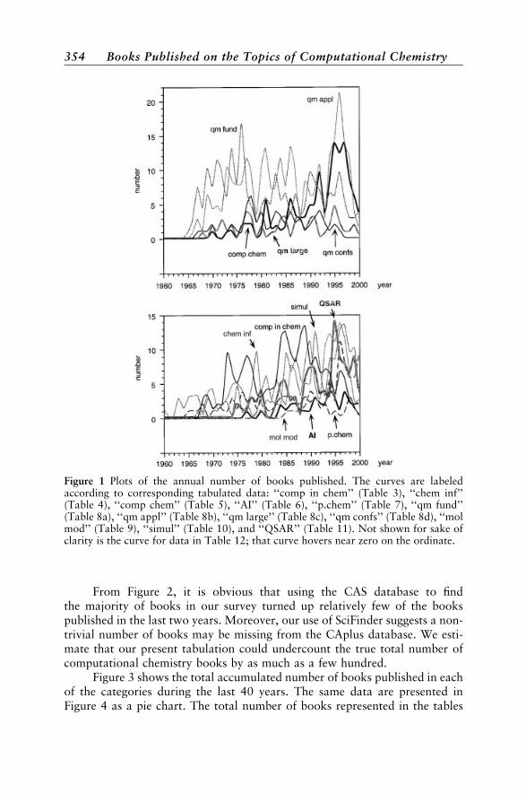
From Figure 2, it is obvious that using the CAS database to findthe majority of books in our survey turned up relatively few of the bookspublished in the last two years. Moreover, our use of SciFinder suggests a non-trivial number of books may be missing from the CAplus database. We esti-mate that our present tabulation could undercount the true total number ofcomputational chemistry books by as much as a few hundred.

Figure 3 shows the total accumulated number of books published in eachof the categories during the last 40 years. The same data are presented inFigure 4 as a pie chart. The total number of books represented in the tables

Figure 1 Plots of the annual number of books published. The curves are labeledaccording to corresponding tabulated data: ‘‘comp in chem’’ (Table 3), ‘‘chem inf’’(Table 4), ‘‘comp chem’’ (Table 5), ‘‘AI’’ (Table 6), ‘‘p.chem’’ (Table 7), ‘‘qm fund’’(Table 8a), ‘‘qm appl’’ (Table 8b), ‘‘qm large’’ (Table 8c), ‘‘qm confs’’ (Table 8d), ‘‘molmod’’ (Table 9), ‘‘simul’’ (Table 10), and ‘‘QSAR’’ (Table 11). Not shown for sake ofclarity is the curve for data in Table 12; that curve hovers near zero on the ordinate.

354 Books Published on the Topics of Computational Chemistry

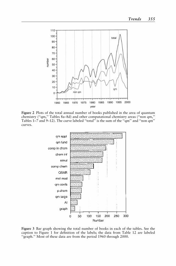
Figure 2 Plots of the total annual number of books published in the area of quantumchemistry (‘‘qm,’’ Tables 8a–8d) and other computational chemistry areas (‘‘non qm,’’Tables 1–7 and 9–12). The curve labeled ‘‘total’’ is the sum of the ‘‘qm’’ and ‘‘non qm’’curves.

Figure 3 Bar graph showing the total number of books in each of the tables. See thecaption to Figure 1 for definition of the labels; the data from Table 12 are labeled‘‘graph.’’ Most of these data are from the period 1960 through 2000.

Trends 355

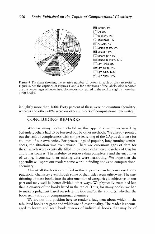
is slightly more than 1600. Forty percent of these were on quantum chemistry,whereas the other 60% were on other subjects of computational chemistry.

CONCLUDING REMARKS

Whereas many books included in this appendix were uncovered bySciFinder, others had to be ferreted out by other methods. We already pointedout the lack of completeness with simple searching of the CAplus database forvolumes of our own series. For proceedings of popular, long-running confer-ences, the situation was even worse. There are enormous gaps of data forthese, which were eventually filled in by more exhaustive searches of CAplusand other sources. The inability to retrieve data completely and the encounterof wrong, inconsistent, or missing data were frustrating. We hope that theappendix will spare our readers some work in finding books on computationalchemistry.

Almost all the books compiled in this appendix can be considered com-putational chemistry even though some of their titles seem otherwise. The par-titioning of these books into the aforementioned categories is subjective on ourpart and may well be better divided other ways. We physically examined lessthan a quarter of the books listed in the tables. Thus, for many books, we hadto make a judgment based on solely the title and/or the author(s) whether thebook really is about computational chemistry.

We are not in a position here to render a judgment about which of thetabulated books are great and which are of lesser quality. The reader is encour-aged to locate and read book reviews of individual books that may be of

Figure 4 Pie chart showing the relative number of books in each of the categories ofFigure 3. See the captions of Figures 1 and 3 for definitions of the labels. Also reportedare the percentages of books in each category compared to the total of slightly more than1600 books.

356 Books Published on the Topics of Computational Chemistry

interest. Citation frequencies can help identify some widely used researchbooks, although equally popular textbooks are not generally heavily cited.The number of copies of each book sold gives an indication of the popularity,but unfortunately publishers are usually loath to reveal their sales data.

We reiterate the caveat that our tabulations, while long, are not compre-hensive. Every effort was made to include as many relevant books as possiblein this appendix, there are probably many books that we overlooked. Thisstatement is especially true for the most recent books, which have not yetbeen cataloged in the CAS database. We apologize to any author or editorwhose book may have been left out; be assured that the omission was inadver-tent, and we regret it. Nonetheless we hope that this tabulation, which is notavailable elsewhere, proves useful to the readers.

REFERENCES

1. D. B. Boyd and K. B. Lipkowitz, in Reviews in Computational Chemistry, K. B. Lipkowitz andD. B. Boyd, Eds., Wiley-VCH, New York, 2000, Vol. 14, pp. 399–439. History of theGordon Research Conferences on Computational Chemistry.

2. P. v. R. Schleyer, N. L. Allinger, T. Clark, J. Gasteiger, P. Kollman, and H. F. Schaefer III, Eds.,Encyclopedia of Computational Chemistry, Vols. 1–5, Wiley, Chichester, 1998.

3. On a technical note, the SciFinder hits were processed and sorted in EndNotes, and then further editedin Microsoft Word.

4. K. B. Lipkowitz and D. B. Boyd, Eds., Reviews in Computational Chemistry, VCH Publishers,New York, 1990, Vol. 1, pp. vii–xii. Preface.

References 357