Review on Micromechanics of Nano‐ and Micro‐Fiber ... COMPOS Review on Micromechanics...Review on Micromechanics of Nano- and Micro-Fiber ... One constituent is called the

Review on Micromechanics of Nano- and Micro-FiberReinforced Composites

Shailesh I. KundalwalApplied and Theoretical Mechanics Laboratory, Discipline of Mechanical Engineering, Indian Institute ofTechnology Indore, Indore 453552, India

This article deals with the prediction of thermome-chanical properties of fiber reinforced compositesusing several micromechanics models. These includestrength of material approach, Halpin–Tsai equations,multi-phase mechanics of materials approaches, multi-phase Mori–Tanaka models, composite cylindricalassemblage model, Voigt–Reuss models, modified mix-ture rule, Cox model, effective medium approach andmethod of cells. Several composite systems reinforcedwith short and long, aligned, random and wavy rein-forcements were considered. In addition, differentaspects such as fiber-matrix interphase, fiber-matrixinterfacial thermal resistance, fiber geometry, and mul-tiple types of reinforcements were considered tomodel the composites systems. The current study alsopresents some important preliminary concepts andapplication of developed micromechanics models toadvanced nanocomposites such as carbon nanotubereinforced composite. Main contribution of the currentwork is the investigation of several analytical microme-chanical models, while most of the existing studies onthe subject deal with only one or two approaches con-sidering few aspects. POLYM. COMPOS., 00:000–000, 2017.VC 2017 Society of Plastics Engineers

INTRODUCTION

A composite is a structural material that consists of two

or more constituents, combined at a macroscopic level and

are not soluble in each other. One constituent is called the

reinforcing phase and the one in which it is embedded is

called the matrix. The reinforcing phase material may be in

the form of fibers, particles, or flakes. Examples of compos-

ite systems include concrete reinforced with steel and epoxy

reinforced with fibers. In addition, advanced composites are

being extensively used in the aerospace industries. These

composites have high performance reinforcements of a thin

diameter in a matrix material such as epoxy-aluminium,

graphite-epoxy, Kevlar-epoxy and boron-aluminium com-

posites. These materials have now found applications in

commercial industries as well [1]. There are many advan-

tages of using composite materials over traditional materials

such as the possibility of weight or volume reduction in a

structure while maintaining a comparable or improved per-

formance level.

Over the last five decades, substantial progress has been

made in the micromechanics of composite materials. One

major objective of micromechanics of heterogeneous mate-

rials is to determine the effective overall properties in terms

of the properties of the constituents and their microstruc-

ture. The most common properties are the thermoelastic

coefficients and thermal conductivities. As outlined by

McCullough [2], numerous micromechanical models have

been developed to predict the macroscopic behavior of

polymeric composite materials reinforced with typical rein-

forcements such as carbon or glass fibers. These microme-

chanical models assume that the fiber, matrix, and

sometimes, the interface, are continuous materials and the

constitutive equations for the bulk composite material are

formulated based on assumptions of continuum mechanics.

Several micromechanical models have been developed

by researchers to predict the effective properties of com-

posites. The earliest works of Voigt [3] and Reuss [4]

were primarily concerned with polycrystals. Their models

can be applied to fiber reinforced composites. Voigt

assumed that the states of strains are constant in the con-

stituents under the application of load. Conversely, Reuss

assumed that the states of stresses are constant in the con-

stituents. Using Voigt and Reuss theories, Hill [5] derived

upper and lower bounds on the effective properties of a

composite material. Likewise, Hashin and Shtrikman [6]

derived upper and lower bounds for the effective elastic

properties of quasi-isotropic and quasi-homogeneous mul-

tiphase materials using a variational approach. Hashin and

Rosen [7] derived bounds and expressions for the effec-

tive elastic moduli of composite materials reinforced with

aligned hollow circular fibers using a variational method.

They obtained the exact results for hexagonal arrays of

identical fibers and approximate results for random array

of fibers. Hill [8, 9] determined the macroscopic elastic

moduli of two-phase composites and showed that the

Correspondence to: S.I. Kundalwal; e-mail: [email protected]

DOI 10.1002/pc.24569

Published online in Wiley Online Library (wileyonlinelibrary.com).

VC 2017 Society of Plastics Engineers

POLYMER COMPOSITES—2017

http://orcid.org/0000-0001-5237-5996

main overall elastic moduli of composites with trans-

versely isotropic phases are connected by simple universal

relations which are independent of the geometry at given

volume fraction. Chamis and Sendeckyj [10] presented a

critique on the theories predicting the thermoelastic prop-

erties of unidirectional fiber reinforced composites. The

theories were considered by them include netting analysis,

mechanics of materials (MOM), self-consistent model,

variational, exact, statistical, discrete element and semi

empirical methods. Several researchers used the

micromechanics-based Mori–Tanaka (MT) method [11] to

predict the effective elastic properties of a composite

material. This method has been successfully applied to

transversely isotropic inclusions by Qui and Weng [12].

Aboudi [13] derived method of cells approaches to pre-

dict the thermoelastic and viscoelastic properties of com-

posites. Several other micromechanical models have also

been developed to determine the overall properties of

composites; these include the self-consistent scheme [14,

15], the generalized self-consistent scheme [16], the dif-

ferential schemes [17, 18], a stepping scheme for multi-

inclusion composites [19], two and three-phase MOM

approaches [20–22], micromechanical damage models

[23], application of multi-phase MT Models [24–28], and

pull-out and shear lag models [29–31].

The method of micromechanical approaches varies

from simple analysis to complex ones. Limited studies

have been reported on the use of most established micro-

mechanical techniques. These studies were either

restricted to few micromechanics models or reported

selected properties taking in to account only special cases.

Therefore, in this study, endeavor has been made to pre-

sent variety of micromechanics techniques characterizing

the effective thermoelastic and thermal properties of

composites considering different influencing parameters

such as fiber structure and orientation, fiber waviness,

fiber-matrix interphase, fiber-matrix interfacial thermal

resistance, and multiple types of reinforcements. This

study provides a concise description and evaluation of

established micromechanical models which are instructive

in the prediction of thermoelastic properties and thermal

properties. The current study provides important insight

in better understanding and judicious application of these

techniques as well as quick and intuitive predictions for

fiber reinforced composites. Preliminary concepts, typical

results, and current trends in nanocomposites are also pre-

sented and discussed herein.

BASIC EQUATIONS

Consider a lamina of fiber reinforced composite mate-

rial as shown in Fig. 1. The 1–2-3 orthogonal coordinate

system is used where the directions are taken as follows:

� The 1-axis is aligned with the fiber axis,

� The 2-axis is in the plane of a lamina and perpendicular to

the fibers, and

� The 3-axis is perpendicular to the plane of a lamina and

thus also perpendicular to the fibers.

The 1-axis is also called the fiber axis, while the 2- and

3-axes are called the matrix directions. This 1-2-3 coordi-

nate system is called the principal material coordinate sys-

tem. The states of stresses and strains in the lamina will be

referred to the principal material coordinate system.

At this level of analysis, the states of stress and strain

of an individual constituent are not considered. The effect

of the fiber reinforcement is smeared over the volume of

the lamina. It is assumed that the fiber-matrix system is

replaced by a single homogenous material. Obviously,

this single material with different properties in three

mutually perpendicular directions is called as orthotropic

material. The Hook’s law for such materials is given by

E11

E22

E33

E23

E13

E12

8>>>>>>>>>>><>>>>>>>>>>>:

9>>>>>>>>>>>=>>>>>>>>>>>;

5

1=E1 2m21=E1 2m31=E3 0 0 0

2m12=E1 1=E2 2m32=E3 0 0 0

2m13=E1 2m23=E2 1=E3 0 0 0

0 0 0 1=G32 0 0

0 0 0 0 1=G13 0

0 0 0 0 0 1=G12

2666666666664

3777777777775

r11

r22

r33

r23

r13

r12

8>>>>>>>>>>><>>>>>>>>>>>:

9>>>>>>>>>>>=>>>>>>>>>>>;

(1)

FIG. 1. A lamina of composite material illustrating representative volume

element (RVE). [Color figure can be viewed at wileyonlinelibrary.com]

2 POLYMER COMPOSITES—2017 DOI 10.1002/pc

where E11, E22, and E33 are the normal strains along 1, 2,

and 3 directions, respectively; E12 is the in-plane shear

strain; E13 and E23 are the transverse shear strains; E1, E2,

and E3 are Young’s moduli along the 1, 2, and 3 direc-

tions, respectively; G12, G23, and G13 are the shear mod-

uli; mij (i, j 5 1, 2, 3) are the different Poisson’s ratios.

Equation 1 can be written in another from as follows

E11

E22

E33

E23

E12

E13

8>>>>>>>>>>><>>>>>>>>>>>:

9>>>>>>>>>>>=>>>>>>>>>>>;

5

S11 S12 S13 0 0 0

S21 S22 S23 0 0 0

S31 S32 S33 0 0 0

0 0 0 S44 0 0

0 0 0 0 S55 0

0 0 0 0 0 S66

2666666666664

3777777777775

r11

r22

r33

r23

r13

r12

8>>>>>>>>>>><>>>>>>>>>>>:

9>>>>>>>>>>>=>>>>>>>>>>>;

(2)

The elements of compliance matrix can be obtained from

Eq. 1. The inverse relation of Eq. 2 is given by

r11

r22

r33

r23

r13

r12

8>>>>>>>>>>><>>>>>>>>>>>:

9>>>>>>>>>>>=>>>>>>>>>>>;

5

C11 C12 C13 0 0 0

C21 C22 C23 0 0 0

C31 C32 C33 0 0 0

0 0 0 C44 0 0

0 0 0 0 C55 0

0 0 0 0 0 C66

2666666666664

3777777777775

E11

E22

E33

E23

E13

E12

8>>>>>>>>>>><>>>>>>>>>>>:

9>>>>>>>>>>>=>>>>>>>>>>>;(3)

In compact form, Eqs. 2 and 3 are written as follows:

Ef g5 S½ � rf g and rf g5 C½ � Ef g (4)

where rf g and Ef g are the stress and stain vectors,

respectively. The inverse of the compliance matrix S½ � is

called the stiffness matrix C½ �.It should be noted that the elastic constants appearing

in Eq. 1 are not all independent. This is clear as the com-

pliance matrix is symmetric. Therefore, we have the fol-

lowing equations relating the elastic constants:

m12

E1

5m21

E2

;m13

E1

5m31

E3

andm23

E2

5m32

E3

(5)

The above equations are called the reciprocity relations.

It should be noted that the reciprocity relations can be

derived irrespective of the symmetry of compliance

matrix. Thus, there are nine independent elastic constants

for an orthotropic material.

A material is called the transversely isotropic if its

behavior in the 2-direction is identical to its behavior in

the 3-direction. For this case: E25E3, m125m13 and

G125G13.

When composite material is heated or cooled, the

material expands or contracts. This is deformation that

takes place independently of any applied load. Let DT be

the change in temperature and let a1, a2, and a3 be the

respective coefficients of thermal expansion for the com-

posite material in the 1, 2, and 3 directions. In such case,

the stress-strain relations can be written as follows:

E112a1DT

E222a2DT

E332a3DT

E23

E13

E12

8>>>>>>>>>>><>>>>>>>>>>>:

9>>>>>>>>>>>=>>>>>>>>>>>;

5

S11 S12 S13 0 0 0

S21 S22 S23 0 0 0

S31 S32 S33 0 0 0

0 0 0 S44 0 0

0 0 0 0 S55 0

0 0 0 0 0 S66

2666666666664

3777777777775

r11

r22

r33

r23

r13

r12

8>>>>>>>>>>><>>>>>>>>>>>:

9>>>>>>>>>>>=>>>>>>>>>>>;

(6)

r11

r22

r33

r23

r13

r12

8>>>>>>>>>>><>>>>>>>>>>>:

9>>>>>>>>>>>=>>>>>>>>>>>;

5

C11 C12 C13 0 0 0

C21 C22 C23 0 0 0

C31 C32 C33 0 0 0

0 0 0 C44 0 0

0 0 0 0 C55 0

0 0 0 0 0 C66

2666666666664

3777777777775

E112a1DT

E222a2DT

E332a3DT

E23

E13

E12

8>>>>>>>>>>><>>>>>>>>>>>:

9>>>>>>>>>>>=>>>>>>>>>>>;(7)

BASIC ASSUMPTIONS

The purpose of this article is to predict the thermome-

chanical properties of a composite material by studying

the micromechanics of the problem. Therefore, in review-

ing models, the current study imposes the general require-

ments that each model must incorporate the effects of

properties of constituents and their volume fractions, fiber

geometry, fiber-matrix interphase, to determine a com-

plete set of properties for the composite. In this regard,

we have the following assumptions:

� both the matrix and fibers are linearly elastic, and the

fibers are either isotropic or transversely isotropic,

� the fibers are continuous, identical in shape and size, and

possess uniform strength,

� the fibers are spaced periodically in square- or hexagonal-

packed arrays (except randomly arranged case),

� the interfacial bond between the neighboring phases is per-

fect, and remains that way during deformation. Thus, the

fiber-interphase-matrix debonding or matrix microcracking

is not considered, and

� the resulting composite is free of voids.

Any model not meeting above-mentioned criteria is

not considered here. Unless otherwise mentioned, the axis

of symmetry of the reinforcement is considered to be

aligned along the 1-axis. When the fibers are uniformly

spaced in the matrix as shown Fig. 1, it is reasonable to

consider a single fiber and the surrounding matrix mate-

rial as the representative volume element (RVE).

DOI 10.1002/pc POLYMER COMPOSITES—2017 3

PRELIMINARIES

Average Stress and Strain

When the composite material is loaded, the point wise

stress field rf g xð Þ and the corresponding strain field Ef gxð Þ will be non-uniform on the microscale. The solution

of these non-uniform fields is a formidable problem.

However, many useful results can be obtained in terms of

average stress and strain [32].

Consider a RVE (V) large enough to contain many

fibers, but small compared to any length scale over which

the average loading or deformation of the composite

varies. The volume average stress �rf g and the volume

average strain �Ef g are defined as the averages of the

point wise stress rf g xð Þ and strain Ef g xð Þ over the vol-

ume, respectively; as follows:

�rf g5 1

V

ðV

rf g xð Þ dV and �Ef g5 1

V

ðV

Ef g xð Þ dV (8)

It is also convenient to define the volume average stresses

and strains for the fiber and matrix phases. To obtain

these, consider the volume (V) which is occupied by the

volume of fibers (Vf) and the volume of matrix (Vm). In

case of two-phase composite, we can write

vf1vm51 (9)

in which vf and vm represent the volume fractions of the

fiber phase and matrix phase in the composite,

respectively.

The average fiber and matrix stresses are the averages

over the corresponding volumes and are given by

�rf� �

51

Vf

ðvf

rf g xð Þ dV and �rmf g5 1

Vm

ðvm

rf g xð Þ dV

(10)

The average strains for the fiber and matrix are defined

similarly.

The relationships between the fiber and matrix aver-

ages, and the overall averages can be derived from the

preceding definitions and these are

�rf g5vf �rf� �

1vm �rmf g (11)

�Ef g5vf �Ef� �

1vm �Emf g (12)

An important related result is the average strain theorem.

Let the average volume (V) subjected to the surface dis-

placements u0� �

xð Þ consistent with the uniform strain

E0� �

. Then the average strain within the region is

�Ef g5 E0� �

(13)

This theorem is proved by Hill [32] by substituting the

definition of the strain tensor Ef g in terms of the

displacement vector uf g into the definition of the average

strain �Ef g and applying Gauss’s theorem. The result is

�Eij

� �5

1

V

ðS

u0i nj1niu

0j

� �dS (14)

where S denotes the surface of V and nf g is a unit vector

normal to dS. The average strain within the volume V is

completely determined by the displacements on the sur-

face of the volume, so the displacements consistent with

the uniform strain must produce the identical value of the

average strain. A corollary of this principle is that, if we

define a perturbation strain Eperf g xð Þ as the difference

between the local strain and average strain as follows

Eperf g xð Þ5 Ef g xð Þ2 �Ef g (15)

then the volume average of Eperf g xð Þ must equal to zero

�Eperf g5 1

V

ðV

Eperf g xð Þ dV50 (16)

The corresponding theorem for the average stress also

holds. Thus, if the surface tractions consistent with r0� �

are exerted on S then the average stress is

�rf g5 r0� �

(17)

Average Properties and Strain Concentration

The objective of the micromechanics models is to pre-

dict the average properties of the composite, but even

these need careful definition. Here, the direct approach by

Hashin [33] was followed, that is, the RVE is subjected

to the surface displacements consistent with the uniform

strain E0� �

. The average stiffness of the composite is the

tensor C½ � that maps this uniform strain to the average

stress:

�rf g5 C½ � �Ef g (18)

The average compliance matrix S½ � is defined in the same

way, applying tractions consistent with the uniform stress

r0� �

on the surface of the average volume:

�Ef g5 S½ � �rf g (19)

Hill [32] introduced an important related concept of strain

and stress concentrations tensors and these are denoted by

M½ � and N½ �, respectively. These are essentially the ratios

between the average fiber strain (or stress) and the corre-

sponding average strain (or stress) in the composite and

are given by

�Ef� �

5 M½ � �Ef g (20)

rf� �

5 N½ � �rf g (21)

where M½ � and N½ � are the fourth-order tensors and, in

general, they must be found from a solution of the


microscopic stress or strain fields. Different microme-

chanics models provide different ways to approximate

M½ � or N½ �. Note that M½ � and N½ � have both the minor

symmetries of the stiffness or the compliance tensor, but

lack the major symmetry. That is,

Mijkl5Mjikl5Mijlk (22)

but in general,

Mijkl 6¼ Mklij (23)

For later use, it will be convenient to have an alternate

strain concentration tensor M� �

that relates the average

fiber strain to the average matrix strain,

�Ef� �

5 M� �

Emf g (24)

This is related to M½ � by

M½ �5 M� �

12vfð Þ I½ �1vf M� �� 21

(25)

in which I½ � represents the fourth-order unit tensor. Using

equations now in hand, one can express the average com-

posite stiffness in terms of the strain concentration tensor

M½ � and the fiber and matrix elastic properties [32]. Com-

bining Eqs. 3, 14, 15, 21, and 23, we can obtain

C½ �5 Cm½ �1vf Cf� �

2 Cm½ ��

M½ � (26)

The dual equation for the compliance is

S½ �5 Sm½ �1vf Sf� �

2 Sm½ ��

N½ � (27)

Equations 26 and 27 are not independent, S½ �5 C½ �21.

Hence, the strain concentration tensor M½ � and stress con-

centration tensor N½ � are not independent either. The

choice of which one to use in any instance is a matter of

convenience.

To illustrate the use of the strain and stress concentration

tensors, we note that the Voigt average corresponds to the

assumption that the fiber and matrix both experience the

same uniform strain. Then �Ef� �

5 �Ef g, M½ �5 I½ �, and from

Eq. 26 the stiffness matrix of the composite is determined as

CVoigt� �

5vf Cf� �

1vm Cm½ � (28)

The Voigt average is an upper bound on the composite stiff-

ness. The Reuss average assumes that the fiber and matrix

both experience the same uniform stress. This implies that

the stress concentration tensor N½ � equals the unit tensor I½ �,and from Eq. 27 the compliance matrix is given by

SReuss� �

5vf Sf� �

1vm Sm½ � (29)

Eigenstrains and Eigenstress

“Eigenstrain” is a generic name given by Mura [34] to

nonelastic strains such as thermal expansion, phase transfor-

mation, initial strains, plastic, misfit strains. “Eigenstress” is

a generic name given to self-equilibrated stresses caused by

one or several of these eigenstrains in bodies which are free

from any other external force and surface constraint. The

eigenstress fields are created by the incompatibility of the

eigenstrains.

For infinitesimal deformations, the total strain ETf g is

regarded as the sum of the elastic strain Ef g and eigen-

strain E�f g,

ETf g5 Ef g1 E�f g (30)

The elastic strain is related to the stress by Hook’s law as

follows

rf g5 C½ � Ef g2 E�f gð (31)

EFFECTIVE THERMOELASTIC PROPERTIES

This section presents the established micromechanics

models for estimating the effective thermoelastic proper-

ties of a composite material containing isotropic or trans-

versely isotropic constituents.

Halpin–Tsai Model (for Isotropic Constituents)

It is well-known fact that the predictions for transverse

Young’s modulus and in-plane shear modulus using strength

of materials approach do not agree well with the experimen-

tal results. This establishes a need for better modeling tech-

niques. These techniques include numerical methods such as

finite element method, boundary element method, elasticity

solution, and variational principal models. Unfortunately,

these models are available only as complicated equations or

in graphical form [10]. Due to these difficulties, semi-

empirical models have been developed for design purposes.

The most useful of these models include those of Halphin

and Tsai [35] because they can be used over a wide range

of elastic properties and fiber volume fractions. Halphin and

Tsai developed their models as simple equations by curve

fitting to results that are based on elasticity. The equations

are semi-empirical in nature because involved parameters in

the curve fitting carry physical meaning.

The Halpin–Tsai equation for the axial Young’s modu-

lus (E1) is same as that obtained through the strength of

materials approach [35],

E15Efvf1Emvm (32)

Transverse Young’s modulus (E2):

E2

Em5

11ngvf

12gvf

(33)

where

g5Ef=Em�

21

Ef=Emð Þ1n(34)


The term n is called the reinforcing factor and it depends

on the fiber geometry, packing geometry and loading con-

ditions. Halpin and Tsai obtained the value of the rein-

forcing factor by comparing Eqs. 33 and 34 to the

solutions obtained from the elasticity solutions. For exam-

ple, for circular fibers in a packing geometry of a square

array, n 5 2. For a rectangular fiber cross section of

length a and width b in a hexagonal array, n 5 2(a/b),

where b is in the direction of loading.

Major Poisson’s ratio (m12):

m125mfvf1mmvm (35)

In-plane shear modulus (G12):

G12

Gm5

11ngvf

12gvf

(36)

where

g5Gf=Gm�

21

Gf=Gmð Þ1n(37)

In this case, for circular fibers in a square array, n 5 1.

For a rectangular fiber cross sectional area of length aand width b in a hexagonal array, n5

ffiffiffi3p

loge a=bð Þ,where a is the direction of loading.

Strength of Materials Approach (for Isotropic Matrix)

This section presents the strength of materials

approach to determine the effective thermoelastic proper-

ties of a composite material made of transversely isotro-

pic fiber and isotropic matrix. Using the strength of

materials approach and simple rule-of-mixtures, we have

the following relations (for a detailed derivation of these

equations the reader is referred to Hyer [36]):

Axial Young’s modulus (E1):

E15Ef1vf1Emvm (38)

Transverse Young’s modulus (E2):

1

E2

5vf

Ef2

1vm

Em

(39)

Major Poisson’s ratio (m12):

m125mfvf1mmvm (40)

In-plane shear modulus (G12):

1

G12

5vf

Gf12

1vm

Gm(41)

Axial coefficient of thermal expansion (CTE) (a1):

a15af

1Ef1vf1amEmvm

Ef1vf1Emvm

(42)

Transverse CTE (a2):

a25a35 af22

Em

E1

� �mf

12 am2af1

� vm

�vf

1 am1Ef

1

E1

� �mm am2af

1

� vf

�vm (43)

We can also use the following rule-of-mixture relation to

determine a2:

a25a35af2vf1amvm (44)

Two-Phase MOM Approach

This section presents the derivation of the microme-

chanics model using the MOM approach [20] to deter-

mine the orthotropic effective elastic properties of a

composite material made of transversely isotropic constit-

uents. To satisfy the perfectly bonding situation between

the fiber and matrix, researchers mainly imposed the iso-

field conditions and used the rules-of-mixture [37, 38].

According to the iso-field conditions one may assume

that the normal strains in the homogenized composite,

fiber and matrix are equal along the fiber direction while

the transverse stresses in the same phases are equal along

the direction transverse to the fiber length. The rules-of-

mixture allows one to express the normal stress along the

fiber direction and transverse strains along the normal to

the fiber direction of the homogenized composite in terms

of that in the fiber and matrix and their volume fractions.

Such iso-field conditions and rules-of-mixture for satisfy-

ing the perfect bonding conditions between the fiber and

matrix can be expressed as

Ef11

rf22

rf33

rf23

rf13

rf12

8>>>>>>>>>>><>>>>>>>>>>>:

9>>>>>>>>>>>=>>>>>>>>>>>;

5

Em11

rm22

rm33

rm23

rm13

rm12

8>>>>>>>>>>><>>>>>>>>>>>:

9>>>>>>>>>>>=>>>>>>>>>>>;

5

E11

r22

r33

r23

r13

r12

8>>>>>>>>>>><>>>>>>>>>>>:

9>>>>>>>>>>>=>>>>>>>>>>>;

(45)

and vf

rf11

Ef22

Ef33

Ef23

Ef13

Ef12

8>>>>>>>>>>><>>>>>>>>>>>:

9>>>>>>>>>>>=>>>>>>>>>>>;

1 vm

rm11

Em22

Em33

Em23

Em13

Em12

8>>>>>>>>>>><>>>>>>>>>>>:

9>>>>>>>>>>>=>>>>>>>>>>>;

5

r11

E22

E33

E23

E13

E12

8>>>>>>>>>>><>>>>>>>>>>>:

9>>>>>>>>>>>=>>>>>>>>>>>;

(46)

In Eq. 46, vf is the volume fraction of the fiber with

respect to the RVE volume (see Fig. 2) and vm 5 12 vf .

Substituting Eq. 3 into Eqs. 45 and 46, the stress and

strain vectors in the composite material can be expressed

in terms of the corresponding stress and strain vectors of

the constituent phases as follows:


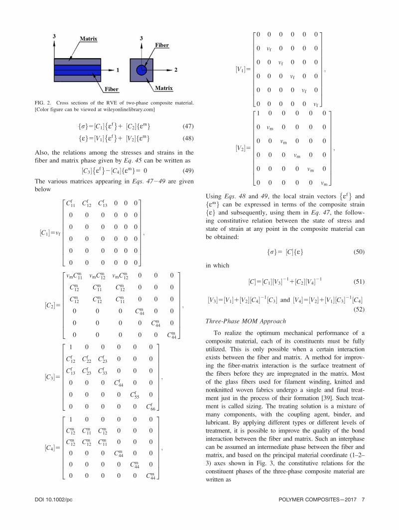
rf g5 C1½ � Ef� �

1 C2½ � Emf g (47)

Ef g5 V1½ � Ef� �

1 V2½ � Emf g (48)

Also, the relations among the stresses and strains in the

fiber and matrix phase given by Eq. 45 can be written as

C3½ � Ef� �

2 C4½ � Emf g5 0 (49)

The various matrices appearing in Eqs. 47249 are given

below

C1½ �5vf

Cf11 Cf

12 Cf13 0 0 0

0 0 0 0 0 0

0 0 0 0 0 0

0 0 0 0 0 0

0 0 0 0 0 0

0 0 0 0 0 0

2666666666664

3777777777775;

C2½ �5

vmCm11 vmCm

12 vmCm12 0 0 0

Cm12 Cm

11 Cm12 0 0 0

Cm12 Cm

12 Cm11 0 0 0

0 0 0 Cm44 0 0

0 0 0 0 Cm44 0

0 0 0 0 0 Cm44

2666666666664

3777777777775;

C3½ �5

1 0 0 0 0 0

Cf12 Cf

22 Cf23 0 0 0

Cf13 Cf

23 Cf33 0 0 0

0 0 0 Cf44 0 0

0 0 0 0 Cf55 0

0 0 0 0 0 Cf66

2666666666664

3777777777775;

C4½ �5

1 0 0 0 0 0

Cm12 Cm

11 Cm12 0 0 0

Cm12 Cm

12 Cm11 0 0 0

0 0 0 Cm44 0 0

0 0 0 0 Cm44 0

0 0 0 0 0 Cm44

266666666664

377777777775;

V1½ �5

0 0 0 0 0 0

0 vf 0 0 0 0

0 0 vf 0 0 0

0 0 0 vf 0 0

0 0 0 0 vf 0

0 0 0 0 0 vf

266666666666664

377777777777775;

V2½ �5

1 0 0 0 0 0

0 vm 0 0 0 0

0 0 vm 0 0 0

0 0 0 vm 0 0

0 0 0 0 vm 0

0 0 0 0 0 vm

266666666666664

377777777777775;

Using Eqs. 48 and 49, the local strain vectors Ef� �

and

Emf g can be expressed in terms of the composite strain

Ef g and subsequently, using them in Eq. 47, the follow-

ing constitutive relation between the state of stress and

state of strain at any point in the composite material can

be obtained:

rf g5 C½ � Ef g (50)

in which

C½ �5 C1½ � V3½ �211 C2½ � V4½ �21

(51)

V3½ �5 V1½ �1 V2½ � C4½ �21 C3½ � and V4½ �5 V2½ �1 V1½ � C3½ �21 C4½ �(52)

Three-Phase MOM Approach

To realize the optimum mechanical performance of a

composite material, each of its constituents must be fully

utilized. This is only possible when a certain interaction

exists between the fiber and matrix. A method for improv-

ing the fiber-matrix interaction is the surface treatment of

the fibers before they are impregnated in the matrix. Most

of the glass fibers used for filament winding, knitted and

nonknitted woven fabrics undergo a single and final treat-

ment just in the process of their formation [39]. Such treat-

ment is called sizing. The treating solution is a mixture of

many components, with the coupling agent, binder, and

lubricant. By applying different types or different levels of

treatment, it is possible to improve the quality of the bond

interaction between the fiber and matrix. Such an interphase

can be assumed an intermediate phase between the fiber and

matrix, and based on the principal material coordinate (1–2–

3) axes shown in Fig. 3, the constitutive relations for the

constituent phases of the three-phase composite material are

written as

FIG. 2. Cross sections of the RVE of two-phase composite material.

[Color figure can be viewed at wileyonlinelibrary.com]


rrf g5 Cr½ � Erf g; r 5 f; i; and m (53)

In Eq. 53, the superscripts f, i, and m denote the fiber,

interphase, and matrix, respectively. Iso-field conditions

and rules-of-mixture [21] for satisfying the perfect bond-

ing conditions between the fiber and neighboring phases

can be expressed as

Ef11

rf22

rf33

rf23

rf13

rf12

8>>>>>>>>>>><>>>>>>>>>>>:

9>>>>>>>>>>>=>>>>>>>>>>>;

5

Ei11

ri22

ri33

ri23

ri13

ri12

8>>>>>>>>>>><>>>>>>>>>>>:

9>>>>>>>>>>>=>>>>>>>>>>>;

5

Em11

rm22

rm33

rm23

rm13

rm12

8>>>>>>>>>>><>>>>>>>>>>>:

9>>>>>>>>>>>=>>>>>>>>>>>;

5

E11

r22

r33

r23

r13

r12

8>>>>>>>>>>><>>>>>>>>>>>:

9>>>>>>>>>>>=>>>>>>>>>>>;

(54)

and

vf

rf11

Ef22

Ef33

Ef23

Ef13

Ef12

8>>>>>>>>>>><>>>>>>>>>>>:

9>>>>>>>>>>>=>>>>>>>>>>>;

1vi

ri11

Ei22

Ei33

Ei23

Ei13

Ei12

8>>>>>>>>>>><>>>>>>>>>>>:

9>>>>>>>>>>>=>>>>>>>>>>>;

1vm

rm33

Em22

Em33

Em23

Em13

Em12

8>>>>>>>>>>><>>>>>>>>>>>:

9>>>>>>>>>>>=>>>>>>>>>>>;

5

r11

E22

E33

E23

E13

E12

8>>>>>>>>>>><>>>>>>>>>>>:

9>>>>>>>>>>>=>>>>>>>>>>>;

(55)

In Eq. 55, vf , vi, and vm represent the volume fractions of

the fiber, interphase, and matrix, respectively, present in

the RVE. Substituting Eqs. 3 into Eqs. 54 and 55, the

stress and strain vectors in the composite material can be

expressed in terms of the corresponding stress and strain

vectors of the constituent phases as follows:

rf g5 C1½ � Ef� �

1 C2½ � Ei� �

1 C3½ � Emf g (56)

Ef g5 V1½ � Ef� �

1 V2½ � Ei� �

1 V3½ � Emf g (57)

C4½ � Ef� �

2 C5½ � Ei� �

5 0 (58)

C5½ � Ei� �

2 C6½ � Emf g 5 0 (59)

The various matrices appearing in Eqs. 56–59 are given

by

C1½ �5

vfCf11 vfC

f12 vfC

f13 0 0 0

Cf12 Cf

22 Cf23 0 0 0

Cf13 Cf

23 Cf33 0 0 0

0 0 0 Cf44 0 0

0 0 0 0 Cf55 0

0 0 0 0 0 Cf66

266666666666664

377777777777775;

C2½ �5vi

Ci11 Ci

12 Ci13 0 0 0

0 0 0 0 0 0

0 0 0 0 0 0

0 0 0 0 0 0

0 0 0 0 0 0

0 0 0 0 0 0

266666666666664

377777777777775;

C3½ �5vm

Cm11 Cm

12 Cm13 0 0 0

0 0 0 0 0 0

0 0 0 0 0 0

0 0 0 0 0 0

0 0 0 0 0 0

0 0 0 0 0 0

26666666666664

37777777777775;

C4½ �5

1 0 0 0 0 0

Cf12 Cf

22 Cf23 0 0 0

Cf13 Cf

23 Cf33 0 0 0

0 0 0 Cf44 0 0

0 0 0 0 Cf55 0

0 0 0 0 0 Cf66

26666666666664

37777777777775;

C5½ �5

1 0 0 0 0 0

Ci12 Ci

22 Ci23 0 0 0

Ci13 Ci

23 Ci33 0 0 0

0 0 0 Ci44 0 0

0 0 0 0 Ci55 0

0 0 0 0 0 Ci66

26666666666664

37777777777775;

C6½ �5

1 0 0 0 0 0

Cm12 Cm

22 Cm23 0 0 0

Cm13 Cm

23 Cm33 0 0 0

0 0 0 Cm44 0 0

0 0 0 0 Cm55 0

0 0 0 0 0 Cm66

26666666666664

37777777777775;

FIG. 3. Cross sections of the RVE of three-phase composite material.

[Color figure can be viewed at wileyonlinelibrary.com]


V1½ �5

1 0 0 0 0 0

0 vf 0 0 0 0

0 0 vf 0 0 0

0 0 0 vf 0 0

0 0 0 0 vf 0

0 0 0 0 0 vf

266666666666664

377777777777775;

V2½ �5

0 0 0 0 0 0

0 vi 0 0 0 0

0 0 vi 0 0 0

0 0 0 vi 0 0

0 0 0 0 vi 0

0 0 0 0 0 vi

266666666666664

377777777777775; and

V3½ �5

0 0 0 0 0 0

0 vm 0 0 0 0

0 0 vm 0 0 0

0 0 0 vm 0 0

0 0 0 0 vm 0

0 0 0 0 0 vm

2666666666664

3777777777775

(60)

Using Eqs. 57–59, the local strain vectors can be

expressed in terms of the composite strain and subse-

quently, using them in Eq. 56, the following effective

elastic coefficient matrix of the composite can be

obtained:

C½ �5 C1½ � V5½ �211 C7½ � V6½ �21

(61)

and

C7½ �5 C3½ �1 C2½ � C5½ �21 C6½ �; V4½ �5 V3½ �1 V2½ � C5½ �21 C6½ �;

V5½ �5 V1½ �1 V4½ � C6½ �21 C4½ � and V6½ �5 V4½ �1 V1½ � C4½ �21 C6½ �(62)

Two-Phase MT Method

MT method [11] is an Eshelby-type model [40] which

accounts for interaction among the neighboring reinforce-

ments. Due to its simplicity, the MT model has been

reported to be the efficient analytical model for predicting

the effective orthotropic elastic properties of composites.

According to the two-phase MT method, the effective

coefficient matrix C½ � of the composite is given by [41]:

C½ �5 Cm½ �1vf Cf� �

2 Cm½ ��

A1½ � (63)

in which

A1½ �5h A½ �i vm I½ �1vf~A1

� �� 21and

h A½ �i5 I½ �1 S½ � Cm½ �ð Þ21 Cf� �

2 Cm½ �� h i21 (64)

where Sf½ � is the Eshelby tensor and it is computed based

on the properties of the matrix and shape of the fiber.

The elements of the Eshelby tensor for the cylindrical

reinforcement in the isotropic matrix are explicitly given

by [12]:

S½ �5

S1111 S1122 S1133 0 0 0

S2211 S2222 S2233 0 0 0

S3311 S3322 S3333 0 0 0

0 0 0 S2323 0 0

0 0 0 0 S1313 0

0 0 0 0 0 S1212

2666666666664

3777777777775

in which

S111150; S22225S33335524mm

8 12mmð Þ ; S22115S33115mm

2 12mmð Þ ;

S22335S332254mm21

8 12mmð Þ ; S11225S113350; S13135S121251=4

and S23235324mm

8 12mmð Þ

Three-Phase MT Method

The effective elastic properties of the composite can

be estimated in the presence of an interphase between a

fiber and the matrix. Using the procedure of the MT

model for multiple inclusions [42], a three-phase MT

model can be derived for the three-phase composite. The

explicit formulation of such three-phase MT model can

be derived as

C½ �5 vm Cm½ � I½ �1 vf Cf� �

Af½ �1vi Ci� �

Ai½ ��

vm I½ �1 vf Af½ �½1 vi Ai½ ��21

(65)

In Eq. 65, vf , vi, and vm represent the volume fractions of

the fiber, interphase, and matrix, respectively with respect

to the RVE of the composite. The concentration tensors

Af½ � and Ai½ � appearing in Eq. 65 are given by

Af½ �5 I½ �1 Sf½ � Cm½ �ð Þ21 Cf� �

2 Cm½ �� n oh i21

(66)

Ai½ �5 I½ �1 Si½ � Cm½ �ð Þ21 Ci� �

2 Cm½ �� n oh i21

(67)

Furthermore, in the above matrices Sf½ � and Si½ � indicate

the Eshelby tensors for the domains f and i, respectively.


For the cylindrical fiber inclusion in the interphase, the

elements of [Sf � can be written as follows:

S111150; S22225S33335524mi

8 12mið Þ ; S22115S33115mi

2 12mmð Þ ;

S22335S332254mi21

8 12mið Þ ; S11225S113350; S13135S121251=4

and S23235324mi

8 12mið Þ

while for the cylindrical fiber-interphase inclusion in the

matrix, the elements of [Si� are given as follows:

S111150; S22225S33335524mm

8 12mmð Þ ; S22115S33115mm

2 12mmð Þ ;

S22335S332254mm21

8 12mmð Þ ; S11225S113350; S13135S121251=4

and S23235324mm

8 12mmð Þ

Using the effective elastic coefficient matrix C½ �, the

effective thermal expansion coefficient vector af g for the

composite can be determined as follows [43]:

af g5 af� �

1 C½ �212 Cf� �21

� �Cf� �21

2 Cm½ �21� �21

af� �

2 amf g�

(68)

where af� �

and amf g are the thermal expansion coeffi-

cient vectors of the fiber and matrix, respectively.

Composite Cylindrical Assemblage Model

The effective elastic moduli of a composite material

reinforced with aligned hollow circular fibers were

derived by Hashin and Rosen [7] using a variational

method. Their model is known as composite cylindrical

assemblage model. Schematic of such model is demon-

strated in Fig. 4. They obtained the following elastic

moduli for hexagonal arrays (see Fig. 5) of identical

fibers reinforced in the matrix.

Axial Young’s modulus (E1):

E15Em vf

Ef

Em1vm

� �Em A12A3B1ð Þ1Ef A22A4B2ð Þ

Em A12A3ð Þ1Ef A22A4ð Þ (69)

A1511a2

12a22mf ; A25

11vg

vm

1vm; A352m2

f

12a2; A45

2m2mvg

vm

;

B15mmvfE

f1mfvmEm

mfvfEf1mmvmEm; B25

mfB1

mm

; a5R1

R2

; vg5R2

2

R2;

vf5 12a2�

vg and vm512vg

(70)

where vg is the volume fraction of the gross cylindrical

inclusion (fiber and the surrounding bonding matrix; see

Fig. 4); R, R1, and R2 are the inner radius of the hollow

fiber, outer radius of the hollow fiber, and radius of gross

cylindrical inclusion, respectively. It may be noted that

the elastic properties of the bonding matrix are same as

those of the matrix.

Longitudinal Poisson’s ratio (m12):

m125EfL1vf1mmEmL2vm

EfL3vf1EmL2vm

(71)

L152mf 12 mmð Þ2h i

vg1vm 11mm½ �mm;

L25 11mf�

a2112mf22 mf� 2

h ivg and

L352 12 mmð Þ2h i

vg1vm 11mm½ � (72)

Longitudinal shear modulus (G12):

G125Gm g 12a2ð Þ 11vg

� 1vm 11a2ð Þ

g 12a2ð Þvm1 11a2ð Þ 11vg

� (73)

where h5Gf=Gm

FIG. 4. RVE of the composite cylindrical assemblage model. [Color

figure can be viewed at wileyonlinelibrary.com]

FIG. 5. Composite cylindrical assemblage made of hexagonal array of

hollow circular fibers. [Color figure can be viewed at wileyonlinelibrary.

com]


Bulk modulus (K23):

K235 �Km

U 12a2ð Þ 112mmvg

� 12mmvm 11 a2

2mf

� �U 12a2ð Þvm1 vg12mm

� 11 a2

2mf

� (74)

where 5�K

f

�Km ; �K

f5kf1Gf ; �K

m5km1Gm; kf5Kf2 2Gf

3;

km5Km2 2Gm

3in which kf and km are the Lame constants

of the fiber and matrix, respectively.

Transverse shear modulus (G23):

Given the complexity of the transverse shear modulus,

the importance of demonstrating the bounding of the solu-

tion is seen. The upper bounds for G23, given by Hashin

and Rosen,7 are

G1ð Þ

23 5Gm 122vg 12mmð Þ �AE

4

122mm

�(75)

where �AE4 can be obtained from the solution of the follow-

ing relation

1 1=vg v2g vg 0 0 0 0

0 2324mm

322mmð Þvg

22v2g

vg

122mm0 0 0 0

1 1 1 1 21 21 21 21

0 2324mm

322mm22

1

122mm0

324mf

322mf2 2

1

122mf

13

322mm23

1

122mm2g 2

3g322mf

3g 2g

122mf

0 21

322mm2 2

1

122mm0

g322mf

22gg

122mf

0 0 0 0 13a2

322mf23=a4 1

122mfð Þa2

0 0 0 0 0 2a2

322mf2=a4 2

1

122mfð Þa2

266666666666666666666666666664

377777777777777777777777777775

�AE1

�AE2

�AE3

�AE4

�BE1

�BE2

�BE3

�BE4

8>>>>>>>>>>>>>>>>>>>>>>>>><>>>>>>>>>>>>>>>>>>>>>>>>>:

9>>>>>>>>>>>>>>>>>>>>>>>>>=>>>>>>>>>>>>>>>>>>>>>>>>>;

5

1

0

0

0

0

0

0

0

8>>>>>>>>>>>>>>>>>>>>>>><>>>>>>>>>>>>>>>>>>>>>>>:

9>>>>>>>>>>>>>>>>>>>>>>>=>>>>>>>>>>>>>>>>>>>>>>>;

The lower bounds for G23, are given by [7]

G2ð Þ

23 5Gm

112vg 12mmð Þ �Ar

4

122mm

h i (76)

where �Ar4 can be obtained from the solution of the following relation

13

322mmð Þvg

23v2g

vg

122mm0 0 0 0

0 21

322mmð Þvg

2v2g 2

vg

122mm0 0 0 0

1 1 1 1 21 21 21 21

0 2324mm

322mm22

1

122mm0

324mf

322mf2 2

1

122mf

13

322mm23

1

122mm2g 2

3g322mf

3g 2g

122mf

0 21

322mm2 2

1

122mm0

g322mf

22gg

122mf

0 0 0 0 13a2

322mf23=a4 1

122mfð Þa2

0 0 0 0 0 2a2

322mf2=a4 2

1

122mfð Þa2

26666666666666666666666666666664

37777777777777777777777777777775

�Ar1

�Ar2

�Ar3

�Ar4

�Br1

�Br2

�Br3

�Br4

8>>>>>>>>>>>>>>>>>>>>>>>>><>>>>>>>>>>>>>>>>>>>>>>>>>:

9>>>>>>>>>>>>>>>>>>>>>>>>>=>>>>>>>>>>>>>>>>>>>>>>>>>;

5

1

0

0

0

0

0

0

0

8>>>>>>>>>>>>>>>>>>>>>>><>>>>>>>>>>>>>>>>>>>>>>>:

9>>>>>>>>>>>>>>>>>>>>>>>=>>>>>>>>>>>>>>>>>>>>>>>;


Method of Cells Approach

This section presents the micromechanics model based

on the method of cells approach to estimate the effective

thermoelastic properties of a composite. Assuming that

fibers are uniformly spaced in the matrix and aligned

along the 1–axis, the resulting composite can be viewed

to be composed of cells forming doubly periodic arrays

along the 2– and 3–directions. Such an arrangement of

cells consisting of subcells is illustrated in Fig. 6. Each

rectangular parallelepiped subcell is labeled by b c, with

b and c denoting the location of the subcell along the 2–

and 3–directions, respectively. The numbers of subcells

present in the cell along the 2– and 3–directions are rep-

resented by M and N, respectively. Here, each cell repre-

sents the RVE and subcell can be either a fiber or the

matrix. Modeling the perfectly bonding condition at the

interface between the subcells is the basis for deriving the

micromechanics model using the method of cells

approach [13]. It may be noted that such perfectly bond-

ing conditions between the subcells can be established by

satisfying the compatibility of displacements and continu-

ities of tractions at the interfaces between the subcells of

the cell. The volume Vbg of each subcell is

Vbc5lbbhc (77)

where bb, hg and l denote the width, height, and length of

the subcell, respectively, while the volume Vð Þ of the cell is

V5lbh (78)

with

b 5XM

b51

bb and h 5XN

c51

hc

The constitutive relations for the medium of a subcell

under thermal environment are given by

rbc� �

5 Cbc� �

Ebc� �

2 abc� �

DT�

(79)

where rbg� �

, Ebg� �

, abg� �

, and Cbg½ � represent the

stress vector, strain vector, thermal expansion coefficient

vector, and elastic coefficient matrix of the subcell,

respectively. It should be noted that to utilize the constit-

uent material properties during computation, the super-

script bc denoting the location of the subcell in the cell

should be replaced by f or m according as the medium of

the subcell is the fiber or the matrix, respectively. In the

method of cells approach, the effective thermoelastic

properties are determined by evaluating the thermoelastic

properties of the repeating cells filled up with the equiva-

lent homogeneous materials. This amounts to volume

averaging of the field variable in concern. Thus, the vol-

ume averaged strain and stress in the composite can be

expressed as follows

Ecf g5 1

V

XM

b51

XN

c51

Vbc Ebc� �

and rcf g5 1

V

XM

b51

XN

c51

Vbc rbc� �

(80)

Here, the superscript c designates the composite. Imposi-

tion of the interfacial displacement continuities provides

the following 2(M 1 N) 1 MN 1 1 number of relations

between the volume averaged subcell strains and the com-

posite strains:

Ebc115Ec

11; b51; 2; . . . :M; c51; 2; . . . :; N (81)

XN

c51

hcEbc225hEc

22; b51; 2; . . . :;M (82)

XM

b51

bbEbc335bEc

33; c51; 2; . . . :;N (83)

XM

b51

XN

c51

bbhcEbc235bhEc

23; (85)

XN

c51

hcEbc125hEc

12; b51; 2; . . . :;M (85)

XM

b51

bbEbc135bEc

13; c51; 2; . . . :;N (86)

Imposition of the interfacial traction continuity conditions

between the adjacent subcells yields the following 5MN –

2(M 1 N) – 1 number of relations between the volume

averaged subcell stresses:

rbc225r b11ð Þc

22 ; b51; 2; . . . :;M21; c51; 2; . . . :; N (87)

rbc335rb c11ð Þ

33 ; b51; 2; . . . :;M; c51; 2; . . . :; N21 (88)

rbc135r b11ð Þc

13 ; b51; 2; . . . :;M21; c51; 2; . . . :; N (89)

rbc125rb c11ð Þ

12 ; b51; 2; . . . :;M; c51; 2; . . . :; N21 (90)

FIG. 6. Representative unit cell of the composite.


rbc235r b11ð Þc

23 ; b51; 2; . . . :;M21; c51; 2; . . . :; N (91)

rbc235rb c11ð Þ

23 ; b51; c51; 2; . . . :; N21 (92)

Equations 81–86 form a set of 2(M 1 N) 1 MN 1 1 num-

ber of relations and can be arranged in a matrix form as

follows:

AG½ � Esf g5 B½ � Ecf g (93)

in which Esf g is the (6MN 31) vector of subcell strains

assembled together and Ecf g is the (6 31) vector of com-

posite strains; AG½ � is the [(2(M 1 N) 1 MN 1 1) 3

(6MN)] matrix formed by the geometrical parameters of

the subcells; and B½ � matrix is constructed by the geomet-

rical parameters of the cell.

Using the constitutive equations given by Eq. 79,

(5MN – 2(M 1 N) – 1) number of traction continuity con-

ditions can be expressed in the following matrix form:

AM½ � Esf g2 asf gDTð Þ50 (94)

in which asf g is the (6MN 3 1) thermal expansion coef-

ficient vector of subcells assembled together and AM½ � is

the [(5MN – 2(M 1 N) – 1) 3 (6MN)] matrix containing

the elastic properties of the subcells. Combination of Eqs.93 and 94 leads to

A½ � Esf g5 K½ � Ecf g1 D½ � asf gDT (95)

where

A½ �5 AM½ �AG½ �

�; K½ �5

�0

B½ �

�and D½ �5 AM½ �

%0

�

with �0 and %0 being [(5MN – 2 M 1 Nð Þ– 1Þ3 6ð )] and

[(2(M 1 N) 1 MN 1 1) 3 (6MN)] null vectors, respec-

tively. From Eq. 95, the subcell strains can be expressed

in terms of the composite strains as follows:

Esf g5 Ac½ � Ecf g1 Dc½ � asf gDT (96)

where Ac½ �5 A½ �21 K½ � and Dc½ �5 A½ �21 D½ �. The matrices

Ac½ � and Dc½ � can be treated as the mechanical and ther-

mal concentration matrices, respectively. It is now possi-

ble to extract the matrices Abgc

� �and Dbg

c

� �of strain

concentration factors for each subcell from the matrices

Ac½ � and Dc½ �, respectively, such that each subcell strains

can be expressed in terms of the composite strains and

thermal strains as follows:

Ebc� �

5 Abcc

� �Ecf g1 Dbc

c

� �asf gDT (97)

Substituting Eq. 97 into Eq. 79 yields

rbc� �

5 Cbc� �

Abcc

� �Ecf g1 Dbc

c

� �asf gDT2 abc

� �DT

� (98)

Using Eq. 97 in Eq. 80, the constitutive relations for the

composite can be derived as

rcf g5 C½ � Ecf g2 af gDTð Þ (99)

in which the effective elastic coefficient matrix C½ � and

effective thermal expansion coefficient vector af g of the

composite are given by

C½ �5 1

V

XM

b51

XN

c51

Vbc Cbc� �

Abcc

� �(100)

af g52C½ �21

V

XM

b51

XN

c51

Vbc Cbc� �

Dbcc

� �asf g 2 abc

� �� (101)

Global Coordinate System

So far, in this work, the constitutive relations for any

material system are written in terms of the thermoelastic

coefficients that are referred to the principal material

coordinate system. The coordinate system used in the

problem formulation, in general, does not always coincide

with the principal coordinate system. Further, composite

laminates have several laminae; each with different orien-

tation. Therefore, there is a need to establish transforma-

tion relations among the thermoelastic coefficients in one

coordinate system to the corresponding properties in

another coordinate system.

In forming composite laminates, fiber reinforced lami-

nae are stacked each other but each having its own fiber

direction. Figure 7 illustrate such rotation of fibers with

respect to the 1-axis.

If the 3-axis of the problem is taken along the laminate

thickness, we have the following transformation law to

relate the thermoelastic coefficients matrices ( �C½ � and �a½ �)in the problem coordinates (10-20-30) to those of C½ � and

af g in the material coordinates (1–2-3):

�C½ �5 T½ �2T C½ � T½ � and �a½ �5 T½ �2T af g (102)

where, T½ �5

m2 n2 0 0 0 2mn

n2 m2 0 0 0 22mn

0 0 1 0 0 0

0 0 0 m n 0

0 0 0 n m 0

2mn mn 0 0 0 m22n2

2666666666664

3777777777775

with

m 5 cos h and n 5 sin h.

Composite Containing Randomly Oriented Fibers

Among various forms of fiber reinforced composites,

sheet molding compound (SMC) appears to be one of the

most promising candidates forming potential applications

in automotive industry because of its relatively low cost

and suitability for high-volume production. The com-

monly used fibers of automotive-type SMC are coated S-


glass filaments. Such glass fibers are randomly dispersed

in a filled or an unfilled thermosetting resin. Considering

different cases, several models were provided herein to

determine the elastic properties of the composite rein-

forced with randomly oriented fibers.

Voigt–Reuss Model. This model estimates Young’s

modulus (EVR) for a lamina of short random fibers and

does not take into account any geometry of the reinforce-

ment. The following relation provides the effective

Young’s modulus:

EVR53

8EA1

5

8ET (103)

where EA and ET are the effective axial and transverse

Young’s moduli of the composite containing aligned

fibers, respectively, and are given by

EA5vfEf1 12vfð ÞEm and ET5

EfEm

Ef 12vfð Þ1vfEm(104)

Halpin–Tsai Model. This model estimates Young’s

modulus (EHR) for a lamina of short random fibers con-

sidering the effect of geometrical parameters of the

reinforcement.

EHT53

8EA1

5

8ET (105)

Various relations appeared in Eq. 105 are given as

follows:

EA5112 Lf=dfð ÞgAvfE

m

12gAvf

; ET5112gTvfE

m

12gLvf

;

gA5Ef=Em�

21

Ef=Emð Þ12 Lf=dfð Þ and gT5Ef=Em�

21

Ef=Emð Þ12

where df and Lf denote the respective diameter and length

of a fiber.

Modified Mixture Law. The formulation of Piggot for

three-dimensional random short fiber composites requires

only three independent variables to estimate Young’s

modulus (EMML):

EMML51

5vfE

f1 12vfð ÞEm (106)

Cox Law. This model [44] incorporates the effect of

aspect ratio of reinforcement into Eq. 106. The following

relation provides Young’s modulus of the composites

reinforced with random short fibers:

ECOX51

512

tan h bsð Þbs

�vfE

f1 12vfð ÞEm 107ð Þ (107)

where s54Lf

df

and b5

ffiffiffiffiffiffiffiffiffiffiffiffiffiffiffiffiffiffiffiffiffiffiffiffiffiffiffiffiffiffiffiffiffiffiffiffiffiffi2pEm

Em 11vmð Þln 1=vfð Þ

s

Randomly Oriented Chopped-Fiber Composites. The

basic constituents of SMC system are resin, filler, fiber

and small amounts of additives. In determining the effec-

tive elastic properties of a typical SMC-composite, the

direct contributions from the additives are ignored and

their weights assigned to the resin weight [45]. By doing

so, a filled SMC can be identified simply as a three-phase

composite (fiber-filler-resin), and an unfilled SMC, a two-

phase composite (fiber-resin).

When the resin and filler are mixed to form the matrix

phase for the final composite, the effective bulk and shear

moduli of the matrix (filled with filler and resin) can be

obtained based on Hashin’s expressions [46] as follows:

Km 5 Kr1 Kp2Krð Þ34Gr13Krð Þv�p

4Gr13Kp13 Kr2Kpð Þv�p(108)

Gm5Gr 1115 12mrð Þ Gp2Grð ÞGrv�p

725mrð ÞGr12 425mrð Þ Gp2 Gp2Grð Þv�ph i

8<:

9=;

(109)

with v�p being the effective filler volume content of the

matrix phase.

v�p5vp

vp1vr

(110)

Young’s modulus and Poisson’s ratio, which are the

effective stiffness properties needed to represent the filled

matrix, can be derived as follows

Em59KmGm

3Km1Gm(111)

mm53Km22Gm

2 3Km1Gmð Þ (112)

Once the effective properties of the filled matrix phase

are known, the three-phase composite can be represented

FIG. 7. Rotation of principal axes from 1 to 2 axes.


as a fiber-matrix mixture. As derived by Hill [8, 14],

axial Young’s modulus and major Poisson’s ratio for the

uniaxial condition are given by:

E15vfEf1vmEm1

4vfvm mf2mm� 2

mm

Kf1 Gf=31 mf

Km1 Gm=31 1

Gm

(113)

m125mfvf1mmvm1 vfvm mf2mm� 1

Km1Gm=32 1

Kf1Gf=3

vm

Kf1Gf=31 vt

Km1Gm=31 1

Gm

!" #

(114)

where the superscript f denotes the fiber, and the matrix

volume fraction (vm) is given by

vm5vr1vp512vf (115)

Based on an elaborate variational principle developed by

Hashin and Shtrikman [7], Hashin [47] obtained the fol-

lowing elastic coefficients.

G23 5Gm 11vf

Gm

Gf2Gm 1Km17

3Gmð Þvm

2 Km143Gmð Þ

8><>:

9>=>;

264

375 (116)

G125 Gm Gf 11vfð Þ1Gmvm

Gfvm1Gm 11vfð Þ (117)

K235Km1Gm

31

vf

1Kf2Km11

3Gf2Gmð Þ1

vm

Km143Gm

( )(118)

The crux of Christensen and Waal’s [48] theory is that the

stiffness of a two-dimensional, randomly oriented fiber com-

posite can be generated from that of transversely isotropic,

unidirectionaly aligned fiber composites by considering the

fibers as evenly oriented from 0 to p. Adopting Cox’s con-

cept of integration, the elastic moduli of a two-dimensional

composite are derived from those of a transversely isotropic,

unidirectionally aligned fiber composite as follows

Pc51

p

ðp

0

P hð Þdh (119)

where Pc represents the elastic moduli of composite mate-

rial and P uð Þ represents the elastic moduli of an unidirec-

tional composite material oriented at an angle u with

respect to the material axis.

Using Hill and Hashin’s results given by Eqs. 113 and

114 and Eqs. 116 to 118, Christensen and Waals applied

the concept of Eq. 119 to obtain the effective elastic

properties of a two-dimensional randomly oriented fiber

composite as follows

Ec51

u1

2 u122u2

2�

(120)

mc5u2

u1

(121)

where Ec and mc denote Young’s modulus and Poisson’s

ratio of the final composite.

u153

8E11

1

2G121

312m121m212

� G23K23

2 G231K23ð Þ (122)

u251

8E12

1

2G121

116m121m212

� G23K23

2 G231K23ð Þ (123)

The final composite density can be expressed by

qc5 qp2qr

� v�pvm1qrvm 1qfvf (124)

The volume fractions of the constituents can be related to

their given weight fractions as follow:

vc5qpqfwr

qpqfwr1qfqrwp1qrqpwr

(125)

vp5qfqrwp

qpqfwr1qfqrwp1qrqpwf

(126)

vf512vr2vp (127)

where wr represents the weight fraction of the rth phase.

Strain Concentration Tensor for Randomly Dispersed

Fibers. It may be noted that the elastic coefficient

matrix C½ � (see Eq. 63) estimated using two-phase MT

method directly provides the effective elastic properties

of the composite, where the fiber is aligned with the 1–

axis. In case of random orientations of fibers, the terms

enclosed with angle brackets in Eq. 64 represent the aver-

age value of the term over all orientations defined by

transformation from the local coordinate system of the

fibers to the global coordinate system. The transformed

mechanical strain concentration tensor for the fibers with

respect to the global coordinates is given by

~Aijkl

� �5tiptjqtkrtls Apqrs

� �(128)

where tij are the direction cosines for the transformation

and are given by

t115cosa cosw sina cosc sinw; t125sina cosw

1cosa cosc sinw;

t135sinw sinc; t2152cosa sinw2sina cosc cosw;

t2252sina sinw1cosa cosc cosw;

t235sinc cosw; t315sina sinc; t3252cosa sinc and

t335cosc

Consequently, the random orientation average of the

dilute mechanical strain concentration tensor h A½ �i can be

determined using the following equation [49]:

h A½ �i5Ð p2p

Ð p0

Ð p=2

0~A� �

a; c; wð Þ sinc dadcdwÐ p2p

Ð p0

Ð p=2

0sinc dadcdw

(129)


where a, g, and w are the Euler angles with respect 1,

2, and 3 axes, respectively. It may be noted that the aver-

aged mechanical strain concentration tensors given by

Eqs. 64 and 129 are used for the cases of aligned and ran-

dom orientations of fibers, respectively, in Eq. 63.

Short Fiber Composite

In the past, various micromechanics models, such as

the dilute concentration model based on the Eshelby’s

equivalent inclusion, the self-consistent model for finite

length fibers, MT models, bounding models, the Halpin–

Tsai equations and shear lag model for estimating the

effective properties of aligned short fiber composites

were reviewed [50]. However, the MT model and Hal-

pin–Tsai equations have been reported to be the efficient

analytical approaches for predicting the effective proper-

ties of short fiber composites [51]. Earlier developed two-

and three-phase MT models in previous sections can be

used directly in property evaluation of short fiber compo-

sites. Therefore, only Halpin–Tsai equations are summa-

rized in the following common form [52]:

P

Pm5

11ngvf

12gvf

(130)

where

g5Pf=Pm�

21

Pf=Pmð Þ11(131)

where P represents any one of the composite elastic mod-

uli listed in Table 1; superscripts f and m refer to the

fiber and matrix, respectively; and n is a parameter that

depends on the Poisson’s ratio of matrix and on the par-

ticular elastic property being considered.

Composite Containing Wavy Fibers

Fiber waviness in composite materials may occur as a

result of a variety of manufacturing induced phenomena.

For example, in filament winding, the winding pressure

can influence the linearity of fibers in underlying layers

[53]. The fiber waviness can be categorized as in-plane or

out-of-plane. In-plane waviness involves the cooperative

undulation of fibers in the plane of the lamina and out-of-

plane waviness generally involves the cooperative undula-

tion of multiple plies through the thickness of laminates

[54]. Generally, in-plane waviness is found to be more

severe than out-of-plane waviness [55]. When fiber wavi-

ness occurs, the mean fiber orientation usually remains

parallel to the desired fiber direction, but displays some

periodic curvature, frequently modeled as sinusoidal

[56–63]. Therefore, the wavy fibers were modeled herein

as sinusoidal fibers; while at any location along its length,

the fiber is considered as transversely isotropic. It may be

noted that the variations of the constructional feature of

the composite can be such that the wavy fibers are copla-

nar with the 1–3 plane or the 2–3 plane as shown in Fig.

8a and b, respectively. In the first, the amplitudes of the

waves are parallel to the plane of a lamina while in the

second, the amplitudes of the wavy fibers are normal to

the plane of a lamina.

The RVE of the composite material containing a wavy

fiber is illustrated in Fig. 9. As shown in this figure, the

RVE is divided into infinitesimally thin slices of thick-

ness dy. Averaging the effective properties of these slices

over the length (LRVE) of the RVE, the homogenized

effective properties of the composite can be estimated.

Each slice can be treated as an off-axis unidirectional

lamina and its effective properties can be determined by

transforming the effective properties of the corresponding

TABLE 1. Parameters to be used in Halpin–Tsai Eqs. 130 and 131 to

predict the effective elastic properties of composite.

P Pf Pm n Comment

G12 Gf Gm 1 Unidirectional short fiber composite

G23 Gf Gm 11mm

32mm24 mmð Þ2 Unidirectional short fiber composite

K23 Kf Km 12mm22 mmð Þ211mm Unidirectional short fiber composite

G Gf Gm 725mm

8210mm Particulate composite

K Kf Km 2 122mmð Þ11mm Particulate composite

FIG. 8. (a) Composite material containing a wavy fiber coplanar with

the plane of a lamina (i.e., 1–3 plane). (b) Composite material contain-

ing a wavy fiber coplanar with the transverse plane of a lamina (i.e., 2–

3 plane). [Color figure can be viewed at wileyonlinelibrary.com]


orthotropic lamina. Now, these wavy fibers are character-

ized by

x5Asin xyð Þ or z5Asin xyð Þ; x5np=LRVE (132)

corresponding to the plane of fiber waviness being copla-

nar with the 1–3 plane and 2–3 plane, respectively. Here,

A and LRVE denote the amplitude of the fiber wave and

linear distance between the fiber ends, respectively; and nrepresents the number of waves of the fiber.

The running length (lnr) of the fiber is given by:

Lnr5

ðLRVE

0

ffiffiffiffiffiffiffiffiffiffiffiffiffiffiffiffiffiffiffiffiffiffiffiffiffiffiffiffiffiffiffiffiffiffiffi11A2x2cos2 xyð Þ

pdy (133)

where the angle a (shown in Fig. 9) is given by

tana5dx=dy5Axcos xyð Þ or tana5dz=dy5Axcos xyð Þ(134)


nar with the 1–3 plane and 2–3 plane, respectively. Note

that for a particular value of x, the value of a varies with

the amplitude of fiber wave.

It may be noted that the effective thermoelastic proper-

ties at any point of any slice of the composite containing

sinusoidally wavy fiber can be approximated by trans-

forming the effective thermoelastic properties of the com-

posite containing straight fibers. It may be noted that

earlier obtained effective thermoelastic tensors ( C½ � and

af g; see Eqs. 51, 61, 63, 65, 68, 100 and 108) are

derived when the fibers are aligned along the 1-axis.

These tensors should be transformed to obtain the proper-

ties when the fibers are aligned along the 3-axis using

Eq. 102. Once Cal� �

and aal� �

are obtained, the effective

elastic coefficient matrix CC½ � and effective thermal

expansion coefficient vector aC� �

at any point of any

slice of the composite can be derived using the appropri-

ate transformations. Transformations for the wavy fibers

being coplanar with the plane of a composite lamina (i.e.,

1–3 plane) are given by:

CC� �

5 T1½ �2T Cal� �

T1½ �21and aC

� �5 T1½ �2T aal

� �(135)

in which

T1½ �5

k2 0 l2 0 kl 0

0 1 0 0 0 0

l2 0 k2 0 2kl 0

0 0 0 k 0 2l

22kl 0 2kl 0 k22l2 2n

0 0 0 l 0 k

2666666666664

3777777777775

k5cos/5 11 npA=LRVEcos npy=LRVEð Þf g2h i21=2

and

l5sin/5npA=LRVEcos npy=LRVEð Þ

11 npA=LRVEcos npy=LRVEð Þf g2h i21=2

Solving Eq. 135, we obtain the following relations

CC115Cal

11k41Cal33l412 Cal

1312Cal55

� k2l2; CC

125Cal12k21Cal

23l2;

CC135 Cal

111Cal3324Cal

55

� k2l21Cal

13 k41l4�

; CC225Cal

22;

CC235Cal

12l21Cal23k2; CC

335Cal11l41Cal

33k412 Cal1312Cal

55

� k2l2;

CC445Cal

44k21Cal66l2; CC

555 Cal111Cal

3322Cal1322Cal

55

� k2l2

1Cal55 k41l4�

;

CC665Cal

44l21Cal66k2; aC

115aal11k21aal

33l2; aC225aal

22 and

aC335aal

11l21aal33k2

The superscript al represents the properties of unidirec-

tional composite lamina in which fibers are aligned along

the 3-direction.

Similarly, if the plane of the fiber waviness is coplanar

with the 2–3 plane, then the effective elastic (CCij ) and

thermal expansion (aCij ) coefficients at any point of the

composite can be determined using the following

transformations:

CC� �

5 T2½ �2T Cal� �

T2½ �21and aC

� �5 T2½ �2T aal

� �(136)

in which

T2½ �5

1 0 0 0 0 0

0 k2 l2 kl 0 0

0 l2 k2 2kl 0 0

0 22kl 2kl k22l2 0 0

0 0 0 0 k 2l

0 0 0 0 l k

2666666666664

3777777777775

Solving Eq. 136, we obtain the following relations

FIG. 9. RVE of the composite material containing a wavy fiber copla-

nar with either the plane of a lamina (i.e., 1–3 plane) or the transverse

plane of a lamina (i.e., 2–3 plane). [Color figure can be viewed at

wileyonlinelibrary.com]


CC115Cal

11; CC125Cal

12k21Cal13l2; CC

135Cal12l21Cal

13k2;

CC225Cal

22k41Cal33l412 Cal

2312Cal44

� k2l2;

CC235 Cal

221Cal3324Cal

44

� k2l21Cal

23 k41l4�

;

CC335Cal

22l41Cal33k412 Cal

2312Cal44

� k2l2;

CC445 Cal

221Cal3322Cal

2322Cal44

� k2l21Cal

44 k41l4�

;

CC555Cal

55k21Cal66l2; CC

665Cal55l21Cal

66k2;

aC115aal

11; aC225aal

22k21aal33l2 and aC

335aal22l21aal

33k2

It is now obvious that the effective thermoelastic proper-

ties of the composite lamina with the wavy fibers vary

along the length of the fiber as the value of a vary over

the length of the fiber. The average effective elastic coef-

ficient matrix �CC

h iand thermal expansion coefficient

vector �aC� �

of the lamina of such composite material

can be obtained by averaging the transformed elastic

CCij

� �and thermal expansion aC

ij

� �coefficients over the

linear distance between the fiber ends as follows [64]:

�CC

h i5

1

LRVE

ðLRVE

0

CC� �

dy and �aC� �

51

LRVE

ðLRVE

0

aC� �

dy

(137)

The Interphase Model

To determine the elastic properties of the interphase,

several models have been implemented in earlier studies

[39, 65–71]. None of these models devoted attention to

model the coefficients of thermal expansion of the inter-

phase layer. The variation in the thermoelastic properties

of the interphase is assumed to satisfy the following

conditions,

Ci� �jr5 Cf� �jr5rf

; Ci� �jr5 Cm½ �jr5ri

; ai� �jr5 af� �jr5rf

and

ai� �jr5 amf gjr5ri

(138)

In Eq. 138, the respective superscripts f, i, and m denote

the fiber, interphase, and matrix. Furthermore, rf is the

fiber radius and ri is the outer radius of the interphase.

Recently, Kundalwal and Meguid [72] proposed a new

interphase model to determine the thermoelastic coeffi-

cients of a nano-tailored composite satisfying the condi-

tions given by Eq. 138. Our model would enable us to

determine the thermoelastic properties of the fiber-matrix

interphase; as follows,

Ci� �jr5 Cm½ � ri

r

� �1

ri2r

ri2rf

� � �g

Cf� �

2 Cm½ � ri

rf

� � �(139)

ai� �jr5 amf g ri

r

� �1

ri2r

ri2rf

� � �g

af� �

2 amf g ri

rf

� � �(140)

where g is the adhesion exponent which controls the qual-

ity of adhesion between a fiber and the surrounding

matrix.

Now, the effective thermoelastic properties of the

interphase can be determined by averaging the varying

interphase properties along radial direction; such that,

Ci� �

51

ri2rf

ðri

rf

Ci� �jr

dr and ai� �

51

ri2rf

ðri

rf

ai� �jr

dr

(141)

Note that the thermoelastic properties of the interphase

were assumed to be vary along the radial direction using

continuity conditions shown in Eq. 138. This assumption

has been used in several studies and validated with exper-

imental and molecular dynamics results to estimate the

interphase properties (see [72] and references therein).

EFFECTIVE THERMAL CONDUCTIVITIES

This section presents established micromechanics models

for estimating the effective conductivities of a composite

material containing either isotropic or orthotropic constituents.

Effective Medium Approach (for Isotropic Constituents)

First, the Maxwell Garnett type effective medium

(EM) approach was presented to estimate the effective

thermal conductivities of the composite material incorpo-

rating the fiber-matrix interfacial thermal resistance. The

EM approach by Nan et al. [73] can be modified to pre-

dict the effective thermal conductivities of the composite

material reinforced with aligned fibers and are given by:

K15vfKf1vmKm (142)

K25K35Km Kf 11að Þ1Km1vf Kf 12að Þ2Km� �

Kf 11að Þ1Km2vf Kf 12að Þ2Km½ � (143)

In Eq. 143, a dimensionless parameter a 5 2ak=df in

which the interfacial thermal property is concentrated on a

surface of zero thickness and characterized by Kaptiza

radius, ak5RkKm where df and Rk represent the diameter

of the fiber and fiber-matrix interfacial thermal resistance,

respectively. The effective thermal conductivity matrix, K½ �,for the composite lamina can be represented as follows

K½ �5

K1 0 0

0 K2 0

0 0 K3

2664

3775 (144)

The effective thermal conductivities ( �K i) at any point in

the composite lamina where the fiber is inclined at an


angle h with the 1–axis (i.e., in 1–2 plane; see Fig. 7) can

be derived in a straightforward manner using the appro-

priate transformation law as follows [74]:

�K½ �5 T1½ �2T K½ � T1½ � (145)

according as the fiber is coplanar with the 1–2 plane (see

Fig. 1) and the corresponding transformation matrix is

given by

T1½ �5

cosh sinh 0

2sinh cosh 0

0 0 1

2664

3775

Composite Cylinder Assemblage Approach (for IsotropicConstituents)

This section presents the composite cylinder assem-

blage (CCA) approach to estimate the effective thermal

conductivities of the composite material. The effective

thermal conductivities of the composite lamina are given

by [75]:

K15vfKf1 12vfð ÞKm (146)

K25K35Km g 11vfð Þ112vf

g 12vfð Þ111vf

�(147)

where g5Kf=Km

Method of Cells Approach (for Orthotropic Constituents)

The MOC approach by Aboudi et al. [76] can be mod-

ified to predict the effective thermal conductivities of the

composite. Assuming that fibers as a rectangular cell, uni-

formly spaced in the matrix and are aligned along the x3–

axis, the composite can be viewed to be composed of

cells forming doubly periodic arrays along the x1– and

x2–directions. Figure 10 shows a repeating unit cell with

four subcells.

Each rectangular subcell is labeled by b c, with b and

c denoting the location of the subcell along the x1– and

x2–directions, respectively. The subcell can be either a

fiber or the matrix. Let four local coordinate systems

(�xbð Þ

1 , �xgð Þ

2 , and x3) be introduced, all of which have ori-

gins that are located at the centroid of each cell. Here,

bb, hg, and l denote the width, height, and length of the

subcell, respectively, while the volume Vð Þ of the repeat-

ing unit cell is

V5bhl (148)

Using MOC approach (for a detailed derivation of these

equations the reader is referred to [76]), the effective

thermal conductivities of the composite lamina are given

by

Kal1 5

Km1 Kf

1 h V111V21ð Þ1h2 V121V22ð Þ½ �1Km1 h1 V121V22ð Þ

� �hbl Km

1 h11Kf1h2

� Kal

2 5Km

2 Kf2 b V111V12ð Þ1b2 V211V22ð Þ½ �1Km

2 b1 V211V22ð Þ� �

hbl Km2 b11Kf

2b2

� and

Kal3 5

Kf3V111Km

3 ðV121ðV211ðV22Þhbl

(149)

The effective thermal conductivities at any point in the

composite where the fiber is inclined at an angle / with

the 3–axis (see Fig. 9) can be derived in a straightforward

manner using the following appropriate transformation

law as follows:

KC� �

5 T1½ �2T Kal� �

T1½ �21and KC

� �5 T2½ �2T Kal

� �T2½ �21

(150)


nar with the 1–3 plane and 2–3 plane, respectively (see

Fig. 8). The various matrices appeared in Eq. 150 are

given by

Kal� �

5

Kal1 0 0

0 Kal2 0

0 0 Kal3

26664

37775; T1½ �5

cos/ 0 sin/

0 0 0

2sin/ 0 cos/

26664

37775 and

T2½ �5

1 0 0

0 cos/ sin/

0 2sin/ cos/

26664

37775;

in which

k5cos/5 11 npA=lfcos npy=lfð Þf g2h i21=2

and

l5sin/5npA=lfcos npy=lfð Þ 11 npA=lfcos npy=lfð Þf g2h i21=2

FIG. 10. Repeating unit cell of the composite material with four sub-

cells (b, c 5 1, 2). [Color figure can be viewed at wileyonlinelibrary.

com]


It is now obvious that the effective thermal conductivities

of the composite lamina containing wavy fibers vary

along the length of the fiber wave as the value of / vary

over its length. The average effective thermal conductiv-

ity matrix of the lamina of such composite containing

wavy fibers can be obtained by averaging the transformed

thermal conductivity coefficients over the linear distance

between the fiber ends as follows:

�KC

h i5

1

LRVE

ðLRVE

0

KC� �

dy (151)

RESULTS AND DISCUSSION

In this section, numerical values of the effective prop-

erties of different composite systems are evaluated using

the different models reviewed in the preceding sections.

For clarity, only the established models were considered

to predict the properties herein. The author also under-

takes some indicative comparisons with respective results

obtained by other researchers. Finally, the application of

micromechanical models has been presented to predict

the properties of carbon nanotube (CNTs) reinforced

composites.

Effective Thermoelastic Properties

The natural questions to ask at this juncture are which

model provides better estimates for thermoelastic proper-

ties of composites. Therefore, comparisons were made

between the results predicted by the different models. The

important associated aspects (fiber-matrix interphase, ran-

dom and wavy orientations of fibers among others) of a

composite in its property evaluation also considered while

comparing the results.

Effect of Interphase. Let us first demonstrate the effect

of fiber-matrix interphase on the effective thermoelastic

properties of the silicon carbide fiber reinforced compos-

ite. For such investigation, the four models were

considered; namely, two- and three-phase MOM

approaches, and two- and three-phase MT methods.

Accordingly, the corresponding Eqs. 51, 61, 63, and 65were used. Carbide fiber, fiber-matrix interphase, and

epoxy matrix are considered for evaluating the numerical

results. Their material properties are listed in Table 2.

Practically, the fiber volume fraction in the composites

can vary typically from 0.3 to 0.7. Hence, this range was

considered to analyze the effect of interphase on the

effective thermoelastic coefficients. Using Eq. 141 and

considering the respective values of adhesion coefficient

(g) and thickness of interphase as 50 and 1 mm, the ther-

moelastic properties of fiber-matrix interphase (see Table

3) were determined. The lower value of g indicates that a

fiber is well bonded to the surrounding matrix through

the intermediate interphase and the reverse is true for the

higher value of g. Values of such adhesion coefficients

can be determined experimentally using Kelly-Tyson

model, Pukanszky model and pull-out model [30]. In sev-

eral studies, the effect of interphase on the nano- and

micro-scale composites was studied, and readers are

referred to Refs. 39, 65–71, 77–80 for more details.

Figure 11 illustrates the variation of the effective elas-

tic coefficient C11 of the carbide fiber reinforced compos-

ite with the carbide fiber volume fraction (vf ). It can be

observed that all the models predict identical estimates. It

is important to note that the fiber-interphase does not

affect the magnitude of C11. Figure 12 illustrates the vari-

ation of the effective elastic coefficient C12 of the com-

posite with the values of vf . It may be observed from Fig.

12 that (i) the MT method overestimates the values of

C12 in comparison to the MOM approach and (ii) the

interphase slightly improves the values of C12 for higher

volume fraction of fiber. As the composite is transversely

isotropic, similar results are also obtained for the effective

elastic coefficient C13 but are not shown here. Similar

trend of results can be observed for the effective trans-

verse elastic coefficient C22 of the composite as shown in

Fig. 13. As the composite is transversely isotropic with

the 1– axis as the symmetry axis, the values of C33 are

TABLE 2. Material properties of the constituent phases of the composite.

Material C11 (GPa) C12 (GPa) C44 (GPa) a1 (1026 K21) (mm)

Silicon carbide fiber [81, 82] 487.61 153.9 166.81 2.4 df 5 150

Fiber-matrix interphase (h550) 16.05 6.36 4.84 50.52 t 5 2

Epoxy matrix [81] 6.57 3.38 1.59 51.15 —

TABLE 3. Material properties of the fiber-matrix interphases.

Adhesion exponent Thickness (mm) C11 (GPa) C12 (GPa) C44 (GPa) a1 (1026 K21)

h55 1 86.76 28.5 29.13 43.14

h55 5 86.82 28.52 29.15 43.58

h510 1 50.32 17.1 16.62 46.86

h510 5 50.4 17.12 16.63 47.41


found to be identical to those of C22 and for brevity are

not presented here. It may be observed from Fig. 14 that

the three-phase MOM approach overestimates the values

of C23 in comparison to the two-phase MOM approach.

Conversely, MT method does not show the influence of

interphase and it over predicts the results in comparison

to the MOM approaches. The MT method significantly

overestimates the values of C55 of the composite as

shown in Fig. 15; but the interphase does not influence

this constant. Figure 16 illustrates the variation of the

axial CTE a1 of the composite with the values of vf . This

figure reveals that the values of a1 decrease with the

increase in the values of vf ; this is obvious result because

the CTE of fiber is much lower than the other two con-

stituents, and therefore, the values of a1 decrease as the

fiber loading in the composite increases. It may also be

observed from Fig. 16 that the interphase does not much

influence the values of a1. Figure 17 demonstrate the

linear decrease in the transverse CTE a2ð Þ of the compos-

ite as the fiber loading in the composite increases. This

figure also demonstrates that the three-phase MOM

approach slightly over predicts the values of a2 in com-

parison to all other models. It may be observed from

Figs. 11–17 that the incorporation of an interphase

between the fiber and matrix slightly increases the trans-

verse thermoelastic coefficients of the resulting compos-

ite; this finding is coherent with the previously reported

results [72, 83–87]. Comparison of the results predicted

by MOM approach with that by the MT methods reveals

that the MOM approach yields conservative estimates;

hence, predictions by the MOM approach have been con-

sidered in the subsequent results for investigating the

effect of interphase thickness and adhesion coefficient on

the effective thermoelastic properties of the composite.

Practically, the fiber-matrix interphase thickness in the

composite can vary; therefore, the investigation of the

FIG. 11. Variation of the effective elastic coefficient C11 of the com-

posite against carbide fiber volume fraction. [Color figure can be viewed

at wileyonlinelibrary.com]











effect of interphase thickness on the effective thermoelas-

tic properties of the composite would be an important

study. For such investigation, two discrete values of inter-

phase thicknesses (t) and adhesion coefficients (g) are

considered: t 5 1, 5 lm and g 5 5, 10. Figures 18–23

illustrate the comparisons of the thermoelastic constants

of the composite for different values of t and g. It may be

observed from these figures that the values of thermoelas-

tic coefficients, except the axial elastic coefficient (C11),

are slightly improved with the increase in the interphase

thickness at higher loading of fibers.

Effect of Random Orientation of Fibers. Practically,

the orientations of the fiber reinforcement in the matrix

can vary over the volume of the composite. Therefore,

studying the properties of composites reinforced with ran-

domly oriented fibers is of a great importance. For such

investigation, carbide fibers are considered to be ran-

domly dispersed in the matrix over the volume of the

composite. First, the effective thermoelastic properties of

the unidirectional fiber reinforced composite were deter-

mined using the two-phase MT method; subsequently, the

transformed mechanical strain concentration tensor given

by Eq. 129 is used to estimate the average properties of

composite containing randomly dispersed fibers. As

expected, this case provides the isotropic thermoelastic

properties for the resulting composite. Figures 24–26

illustrate the variations of the effective thermoelastic

coefficients of the composite with the fiber loading.

These results clearly demonstrate that the randomly dis-

persed fibers improve the values of C12, C22, and a1 of

the composite over those of the values of C12, C22, and

a1 of the composite reinforced with aligned fibers (see

Figs. 12 and 13); the respective improvements are found




FIG. 16. Variation of the axial CTE a1 of the composite against car-

bide fiber volume fraction. [Color figure can be viewed at wileyonlineli-

brary.com]

FIG. 17. Variation of the transverse CTE a2 of the composite against

carbide fiber volume fraction. [Color figure can be viewed at wileyonli-

nelibrary.com]

FIG. 18. Effect of interphase thickness on the effective elastic coeffi-

cient C11 of the three-phase composite. [Color figure can be viewed at



to be 470%, 600%, and 74% when the fiber loading is

0.7. Conversely, it may be observed that the random ori-

entations of fibers significantly affect the effective CTEs

of the composite. The improvement in the elastic proper-

ties is attributed to the fact that the fibers are homoge-

neously dispersed in the matrix in the random case, and

hence, the overall elastic properties of the resulting com-

posite improve in comparison to the aligned case.

Effect of Waviness of Fibers. The effect of fiber wavi-

ness on the effective thermoelastic properties of the com-

posite is investigated when wavy fibers are coplanar with

either of the two mutually orthogonal planes. It may be

noted that the axis symmetry of carbide fibers is consid-

ered to be aligned along the 3–direction (see Figs. 8 and

9); accordingly, the transformations for the wavy fibers

being coplanar with the 1–3 plane or the 2–3 plane are

carried out. The effect of fiber waviness is studied by

varying the value of fiber wave frequency, x5np=Ln; the

multiplying factor (n) takes the value from 0 to 24 and

the amplitude (A) of the fiber wave is considered as 75

mm. Figure 27 illustrates the variations of the values of

C11 of the composite with the wave frequency. It may be

observed from Fig. 27 that the value of C11 significantly

increases as the value of x increases when the wavy

fibers are coplanar with the 1–3 plane but the values of

C11 are not much influenced by the wavy fibers being

coplanar in the 2–3 plane. Although not shown here, the

same trend of results is obtained for the values of C12.

Conversely, it may be observed from Fig. 28 that the val-

ues of C22 significantly increase as the value of xincreases when the wavy fibers are coplanar with the 2–3

plane but the values of C22 are not much influenced by

the wavy fibers being coplanar in the 1–3 plane. Similar










FIG. 22. Effect of interphase thickness on the effective axial CTE a1

of the three-phase composite. [Color figure can be viewed at wileyonli-

nelibrary.com]


trend of results has been obtained for the values of C23 as

shown in Fig. 29. Figure 30 demonstrates that the value

of C55 significantly enhances when the wavy fibers are

coplanar with the 1–3 plane. As the composite is trans-

versely isotropic material, the values of C66 are found to

be identical to those of the values of C55. Figures 31 and

32 demonstrate the variations of the values of a1 and a2

of the composite with the wave frequency. These figures

reveal that the values of a1 and a2 increase with the

increase in the values of x when the wavy fibers are

coplanar with the 1–3 plane and 2–3 plane, respectively.

It may be noted from Figs. 27–32 that if the wavy fibers

are coplanar with the 1–3 plane then the axial thermoelas-

tic coefficients of the composite are significantly

improved. When the wavy fibers are coplanar with the

plane 1–3 as shown in Fig. 8a, the amplitudes of the fiber

waves become parallel to the 1–axis and this results into

the aligning of the projections of parts of fibers lengths

with the 1–axis leading to the axial stiffening of the com-

posite. The more is the value of x, the more will be such

projections and hence the effective axial thermoelastic

coefficients (C11, C12, C13, C55, C66, and a1) of the com-

posite increase with the increase in the values of x. Con-

versely, if the wavy fibers are coplanar with the

transverse plane (2–3 plane) then the transverse thermo-

elastic coefficients (C22, C23, C33, C44, a2, and a3) of the

composite are improved.

Application of Micromechanics Models toNanocomposites

Polymer nanocomposites embedded with nanoparticles

such as CNTs, graphene and their derivatives, nanoclays,

and silica nanoparticles have attracted a large amount of

FIG. 23. Effect of interphase thickness on the effective transverse CTE

a2 of the three-phase composite. [Color figure can be viewed at


FIG. 24. Variation of the effective elastic coefficient C11 (or C22) of

the composite containing randomly dispersed fibers. [Color figure can

be viewed at wileyonlinelibrary.com]

FIG. 25. Variation of the effective elastic coefficient C12 (or C23) of

the composite containing randomly dispersed fibers. [Color figure can

be viewed at wileyonlinelibrary.com]

FIG. 26. Variation of the effective CTE a1 (or a2) of the composite

containing randomly dispersed fibers. [Color figure can be viewed at



attention to achieve more improved thermomechanical

properties than conventional composites [88–98]. Among

all others, CNTs [99] have been emerged as the ideal can-

didates for multifarious applications due to their remark-

able thermoelastic and physical properties. The quest for

utilizing the remarkable thermomechanical properties of

CNTs [86, 100–102] has led to the emergence of a new

area of research that involves the development of nano-

composites [103–113]. These studies revealed that the

addition of a small fraction of CNTs into a polymer

matrix introduces significant improvement in the multi-

functional properties of microcomposites and nanocompo-

sites. Therefore, the current study endeavored to utilize

the micromechanics models for estimating the thermoelas-

tic properties of CNT-reinforced nanocomposites herein.

Thermoelastic Properties. The performance of a CNT-

reinforced nanocomposite material is critically controlled

by the interfacial bonding between a CNT and the sur-

rounding matrix material. Chang et al. [114] used Raman

scattering and X-ray diffraction techniques, and showed

that no chemical bonding exists between a CNT and the

surrounding polymer matrix. In this case, only the domi-

nating non-bonded van der Waals (vdW) interactions can

be considered between a CNT and the surrounding poly-

mer matrix [115–117]. To estimate the effective thermo-

elastic properties of the CNT-reinforced composite, the

consideration of vdW interactions between a CNT and

the surrounding polymer matrix, is an important issue. In

several research studies [86, 103], an equivalent solid

continuum interphase was considered between a CNT and

FIG. 27. Effect of waviness of fiber on the effective elastic coefficient

C11 of the composite (x5np=Ln; n 5 0 to 24). [Color figure can be

viewed at wileyonlinelibrary.com]











the polymer matrix which characterizes vdW interactions;

this assumption allows us to use the interphase model uti-

lized in the current study for estimating the thermoelastic

properties of the CNT-matrix interphase. The results pre-

dicted by the interphase model were compared with the

predictions of molecular dynamics simulations carried out

by Tsai et al. [86]. In their study, the thickness of the

interphase (hi) was assumed equal to the non-bonded gap,

and the corresponding elastic properties were determined

from the molecular energy calculated from molecular

dynamics simulations. Tsai et al. [86] determined

Young’s modulus of the interphase from the normalized

non-bonded energy in CNT-polyimide nanocomposite

considering three different types of zigzag CNTs. For the

comparison purpose, transversely isotropic elastic proper-

ties of zigzag CNTs are taken from Tsai et al. [86] and

the elastic properties of the polymer material are taken

from Odegard et al. [103]. In Table 4, the predicted

Young’s modulus of the interphase considering adhesion

coefficient (g) as 40 are compared with the existing

molecular dynamics simulations.

With CNT type varying from (10, 0) to (18, 0), these

comparisons reveal that: (i) the interphase model accu-

rately predicts Young’s modulus of the interphase for the

CNT (14, 0) and (ii) over predicts Young’s modulus of

the interphase for a smaller diameter of CNT and (iii)

under predicts the same for larger diameter of CNT. The

marginal differences observed are attributed to the fact

that the polyimide polymer is generated by 10 repeated

monomer units in the study of Tsai et al. [86], whereas in

the interphase model, the elastic properties of the polyi-

mide material are taken from Odegard et al. [103]. Thus,

it can be inferred from these comparisons that the inter-

phase model can be reliably applied to predict the ther-

moelastic properties of the interphase if the value of CNT

diameter is between 1 and 1.4 nm and the value of g is

40.

It is accepted by many researchers that CNT-

reinforced composites can be considered as fiber rein-

forced composites so that their elastic properties can be

predicted using the available micromechanics methods.

Seidel and Lagoudas [83] estimated the effective elastic

properties of CNT-reinforced composites using the self-

consistent and the MT methods. Song and Youn [118]

numerically estimated the effective elastic properties of

CNT-reinforced polymer-based composites using the

homogenization technique. The control volume finite ele-

ment method is adopted in their study to implement the

homogenization method with the assumption that the

CNT-epoxy nanocomposites have geometrical periodicity

with respect to a microscopic scale. Recently, Farsadi

et al. [119] developed a three-dimensional finite element

model to investigate the effect of CNT volume fraction

and waviness on the mechanical properties of nanocom-

posites reinforced with waved CNT. They reported that

the CNT waviness decreases the axial and transverse

Young’s moduli of nanocomposites but the change in the

value of transverse Young’s modulus is less remarkable

than the axial Young’s modulus. Suggestive literature

indicates that the established micromechanics models can

be utilized to determine the effective properties of CNT-

reinforced nanocomposites. Therefore, the MT method

was utilized herein to determine the effective thermoelas-

tic properties of CNT-reinforced nanocomposites and the

obtained results were compared with those of the obtained

by Farsadi et al. [119]. Table 5 summarizes the outcome

of this comparison. The two sets of results predicted by

the finite element and the MT model are in excellent

agreement, validating the later.

To further show the applicability of the MT method,

the effective CTEs of the CNT-reinforced nanocomposite

predicted by the MT method are compared with the finite

element predictions of the nanocomposite containing

FIG. 31. Effect of waviness of fiber on the effective axial CTE a1 of

the composite (x5np=Ln; n 5 0 to 24). [Color figure can be viewed at


FIG. 32. Effect of waviness of fiber on the effective axial CTE a2 of

the composite (x5np=Ln; n 5 0 to 24). [Color figure can be viewed at



straight CNTs. Kirtania and Chakraborty [120] deter-

mined the CTEs of the aligned CNT-reinforced nanocom-

posite using the finite element model. For the comparison

purpose, CNTs and matrix material of the nanocomposite

studied by Kirtania and Chakraborty [120] are considered

for the constituent phases of the nanocomposite. For the

effective CTEs of the CNT-reinforced nanocomposite, the

two sets of results are in excellent agreement as demon-

strated in Table 6.

Thermal Conductivities. In this section, the effective

thermal conductivities of CNT-reinforced nanocomposite

are presented using the EM and the CCA approaches.

The current predictions are also compared against those

from the experimental results by Marconnet et al. [121].

They fabricated the aligned CNT-polymer nanocompo-

sites consisting of CNT arrays infiltrated with an

aerospace-grade thermoset epoxy. For the comparison

purpose, the values of thermal conductivities of the CNT

and polymer matrix are taken as Kn522:1 W=mK and

Kp50:26 W=mK, respectively, as considered by Marcon-

net et al. [121]. The comparisons of the axial (KA) and

transverse (KT) thermal conductivities of the aligned

CNT-polymer nanocomposites estimated by the EM and

CCA approaches with those of the experimental results

are illustrated in Figs. 33 and 34, respectively. In these

figures, dotted blue line represents best fits obtained from

the EM approach for the experimental results considering

an alignment factor (AF) of CNTs as 0.77 observed from

the scanning electron microscopy. Figure 33 reveal that

the values of KA predicted by the EM and CCA

approaches overestimate the values of KA by 20% and

25% when the values of CNT volume fractions are 0.07

and 0.16, respectively. Conversely, the EM and CCA

approaches underestimate the values of KT by 40% and

58% when the values of CNT volume fractions are 0.07

and 0.16, respectively. These differences between the

results are attributed to the fact that the perfect align-

ments of CNTs (i.e., AF 5 1) are considered while com-

puting the results by the EM and CCA approaches

whereas the value of AF is 0.77 in Ref. 124. Other possi-

ble reasons for the disparity between the analytical and

experimental results include the CNT-matrix interfacial

thermal resistance [121, 122], lattice defects within CNTs

[123], and modification of the phonon conduction within

CNTs due to interactions with the matrix [124]. It can be

inferred from the comparisons shown in Figs. 33 and 34

TABLE 4. Comparison of Young’s moduli of the CNT-polymer matrix interphase.

CNT type Diameter of CNT (nm) hI (nm)

E (Gpa) E (GPa)

Molecular dynamics simulation [86]

Mori–Tanaka Present modela (g 5 40)

(10, 0) 0.78 0.3333 19.23

17.800

21.90

4.448

(14, 0) 1.1 0.3236 17.95

17.790

17.92

4.44

(18, 0) 1.42 0.3158 17.90

17.800

15.65

4.446

aIn this validation example, Young’s modulus (Ep) and the Poisson’s ratio (mp) of the polymer matrix are consedered as 3.8 GPa and 0.4, respectively

[103].

TABLE 5. Comparison of the engineering constants of the CNT-

reinforced nanocomposite containing sinusoidally wavy CNTs.

w5A=k

Eyy (GPa) Exx (GPa)

FE model [119] MT model FE model [119] MT model

0 18 17.800 4.577 4.448

0.005 17.920 17.790 4.574 4.448

0.010 17.780 17.800 4.570 4.446

0.015 17.690 17.750 4.566 4.445

0.020 17.570 17.720 4.563 4.442

0.025 17.480 17.680 4.561 4.440

0.030 17.130 17.630 4.559 4.435

Farsadi et al. [119]: En51; 030 GPa, mn50:063, Ep53:8 GPa, mp50:4

and CNT volume fraction, vn50:014; where w is the waviness ratio; A

and k are the amplitude and the wave length of CNT wave; En and mn

are the Young’s modulus and Poisson’s ratio of the CNT. Eyy and Exx

are the axial and transverse Young’s moduli of the nanocomposite,

respectively.

TABLE 6. Comparison of the CTEs of the CNT-reinforced nanocom-

posite containing straight CNTs.

a1 31026 K21�

a2 31026 K21�

vn FE Model [120] MT Model FE Model [120] MT Model

0.5 25.2030 24.4850 69.7540 69.9030

1 15.3020 15.0720 72.8670 72.8790

3 5.0978 5.1820 74.7155 74.5120

5.45 2.2670 2.2978 73.5434 73.1220

7.9 1.0643 1.1170 71.7165 71.1300

10.3 0.4253 0.4847 69.7879 69.0140

15.77 20.3201 20.2560 65.1728 64.0370

Kirtania and Chakraborty [120]: En51; 000 GPa, mn50:2, Ep53:89

GPa, mp50:37, an521:531026K21, and ap55831026K21; where a1

and a2 are the axial and transverse CTEs of the nanocomposite with the

straight CNTs, respectively; an and ap are the CTEs of the CNT and

the polymer matrix, respectively.


that the EM and CCA approaches can be reasonably

applied to predict the thermal conductivities of the CNT-

reinforced nanocomposites.

Advanced Nanocomposites. Literature on hybrid com-

posites indicate that the use of CNTs and conventional

fibers together, as multiscale reinforcements, significantly

improves the overall properties of resulting hybrid com-

posites, which are unseen in conventional composites.

More success can be achieved in improving the multi-

functional properties of the hybrid composites by growing

CNTs on the surfaces of conventional fibers. For instance,

a novel nano-reinforced laminated composite (NRLC),

containing carbon fibers grown with the CNTs, has been

characterized experimentally and numerically by Kulkarni

et al. [104]. The longitudinal and transverse cross sections

of such NRLC are shown schematically in Fig. 35.

Therefore, to show the applicability of microme-

chanics models to advanced composites, the results pre-

dicted by the MT method are compared with those of

numerical and experimental findings on the NRLC. The

constituent phases as well as the geometrical parameters

of the NRLC studied by Kulkarni et al. [104] are con-

sidered for the comparison purpose. Table 7 demon-

strates the comparison between the two sets of results

for the NRLC. It may be observed from Table 7 that

the predicted value of the transverse Young’s modulus

(Ex) of the NRLC computed by the MT method match

closely with that of the experimental value. The experi-

mental value of Ex is lower than the theoretical predic-

tion, and this is attributed to the fact that CNTs are not

perfectly radially grown and straight, and hence, the

radial stiffening of the NRLC decreases [104]. It may

also be noted that the value of Ex predicted by the MT

method is much closer to the experimental value than

that of the numerical value predicted by Kulkarni et al.

[104]. These comparisons are significant as the predic-

tion of the transverse Young’s modulus of the NRLC

provides critical check on the validity of the MT

method. Thus, it can be inferred from the comparisons

shown in Table 7 that the micromechanics models can

be reliably applied to predict the overall thermoelastic

properties of the advanced composite.

FIG. 33. Comparisons of the variations of the effective axial thermal

conductivities of the aligned CNT-reinforced polymer nanocomposite

(#[121]). [Color figure can be viewed at wileyonlinelibrary.com]

FIG. 34. Comparisons of the variations of the effective transverse ther-

mal conductivities of the aligned CNT-reinforced polymer nanocompo-

site (#[121]). [Color figure can be viewed at wileyonlinelibrary.com]

FIG. 35. Transverse and longitudinal cross sections of the NRLC

[104].

TABLE 7. Comparison of the effective engineering constants of the

NRLC [104] with those of the CNT-reinforced nanocomposite.

NRLC (2% CNT and 41% IM7

carbon fiber)

Numerical Experimental MT model

Ex(GPa) 13.93 10.02 11.91

mxy 0.34 — 0.38

mzx 0.16 — 0.18


SUMMARY

This article reviews and evaluates several microme-

chanics models that predict the thermomechanical properties

of nano- and micro-fiber reinforced composite materials.

The overall goal of this work is to provide quick and intui-

tive property predictions for different composite systems

using established analytical micromechanical models. To

investigate the effect of reinforcement on the thermome-

chanical properties, different cases of reinforcements are

considered: aligned, random, and wavy. Specific attention

was given to investigate the effect of fiber waviness on the

effective thermoelastic properties of composite when wavy

fibers are coplanar with either of the two mutually orthogo-

nal planes. The current study shows the application of inter-

phase model, which is developed by the current author in

his previous work, to predict the thermoelastic properties of

fiber-matrix interphase. This work also shows the applicabil-

ity of established micromechanics models to predict the

properties of CNT-reinforced composites considering the

non-bonded interactions between a CNT and the polymer

matrix as an equivalent solid continuum. The results from

the micromechanics models are validated with the existing

numerical and experimental findings on the nanocomposites

and found to be in good agreement. The following is a sum-

mary of findings of the current study:

1. MOM approach yields conservative estimates compared to

the MT approach,

2. pronounced effect of fiber-matrix interphase on the effec-

tive transverse thermoelastic coefficients of the fiber rein-

forced composite is observed at higher volume fraction of

fibers,

3. randomly oriented fibers have significant influence on the

thermoelastic properties of the composite,

4. the transverse thermoelastic coefficients of composites

reinforced with aligned fibers are less than those of the

randomly dispersed case,

5. significant improvement has been observed in the effec-

tive thermoelastic properties of the composite when wavy

fibers are coplanar with either of the two mutually orthog-

onal planes; the axial and transverse thermoelastic proper-

ties of a composite improve when wavy fibers are

coplanar with the plane of a lamina and the transverse

plane of a lamina, respectively, and

6. the modeling strategy developed herein is capable of

determining the effective thermoelastic properties and

thermal conductivities of any advanced composite contain-

ing aligned or randomly dispersed nano- and micro-fibers

with less computational efforts.

ABBREVIATIONS

A Amplitude of the fiber, m

ak Kaptiza radius, m

A½ � Matrix formed by the geometrical parame-

ters and the material properties of the

subcell

Ar½ � Strain concentration tensor for the rth phase

Ac½ � Matrix containing strain concentration fac-

tors of all the subcells

Abgc

� �Strain concentration matrix of the bcth

subcell

AG½ � Matrix constructed by the geometrical

parameters of all the subcells

Am½ � Matrix containing the elastic properties of

all the subcells,

b Width of the subcell

B½ � Matrix constructed by the geometrical

parameters of the cell,

CCA Cylinder assemblage approach

CTE Coefficient of thermal expansion�C

Ch i

Elastic coefficient matrix of the composite

containing wavy fibers, GPa

Cr½ � Elastic coefficient matrix of the rth phase,

GPa

Cbg½ � Elastic coefficient matrix of the bcth sub-

cell, GPa

Crij Elastic coefficients of the rth phase, GPa

Cbgij Elastic coefficients of the bcth subcell, GPa

df Diameter of the fiber, m

Dc½ � Thermal concentration matrix of all the

subcells

Dbgc

� �Thermal concentration matrix of the bcth

subcell

EA and ET Effective axial and transverse Young’s

moduli of the composite containing aligned

fibers, respectively, GPa

Ec and mc Young’s modulus and Poisson’s ratio of a

two-dimensional randomly oriented

composite

Er Young’s modulus of the rth phase, GPa

E1, E2, E3 Young’s modulus referred to the principal

material coordinate (1–2–3) axis, GPa

Gr Shear modulus of the rth phase, GPa

G12, G13 Axial shear moduli, GPa

G23 Transverse shear modulus, GPa

h Height of the subcell, m

I½ � Fourth-order identity matrix

K23 Effective bulk modulus, GPa

Kr Thermal conductivity of the rth phase, W/

mK

L Length of the unit cell, m

Lf Length of the fiber

Lnr Running length of the sinusoidally wavy

fiber, m

LRVE Length of the RV m

M Number of subcells present in the cell along

the 1 – direction

M½ � Strain concentration tensor

M� �

Alternate strain tensor that relate the aver-

age fiber strain to the average matrix strain,

MOC Method of cells,

MOM Mechanics of materials,


MT Mori–Tanaka

N Number of subcells present in the cell along

the 2– direction

N½ � Stress concentration tensor

n Number of waves of the sinusoidally wavy

fiber along its axial direction

nf g Unit vector

K1, K2, K3 Thermal conductivity referred to the princi-

pal material coordinate (1–2–3) axis, W/mK

Rk Interfacial thermal resistance between the

fiber and matrix, m2K/W

rr Radius of the rth phase, m,

RVE Representative volume element

Sr½ � Elastic compliance matrix of the rth phase

Srij Elements of compliance matrix of the rth

phase

S½ � Eshelby tensor

Sijkl Elements of Eshelby tensor,

SMC Sheet molding compound

T½ � Transformation matrix

V Volume of the RVE of the composite

Vr Volume of the rth phase

vr Volume fraction of the of the rth phase

Vbg Volume of the bcth subcell m3ð Þwr Weight fraction of the rth phase, kg

af g Thermal expansion coefficient vector of the

composite, K21

arf g Thermal expansion coefficient vector of the

rth phase, K21

ai Thermal expansion coefficients of the com-

posite, K21

abg� �

Thermal expansion coefficient vector of the

bcth subcell, K21

DT Temperature deviation from the reference

temperature, K

Ef g Strain vector�Ef g Volume average strain vector

E�f g Eigenstrain vector

E0� �

Uniform strain vector

Eperf g Perturbation strain vector

Erf g Strain vector of the rth phase

ETf g Total strain vector

‹bg� �

Strain vector of the bcth subcell

Er1, Er

2, Er3 Normal strains along the principal material

coordinate axes 1, 2, and 3, respectively, in

the rth phase

Er12, Er

13, Er23 Shearing strains in the rth phase,

g Adhesion exponent

k Wavelength of the fiber, m

m12, m13, m23 Poisson’s ratios

mf , mi & mp Poisson’s ratios of the fiber, interphase, and

matrix, respectively,

n Reinforcing factor

qr Density of the rth phase, kg/m3

rf g Stress vector, GPa

�rf g Volume average stress vector, GPa

r0� �

Uniform stress vector, GPa

rrf g Stress vector of the rth phase, GPa

rbg� �

Stress vector of the bcth subcell, GPa

rr1, rr

2, rr3 Normal stresses along the principal material

coordinate axes 1, 2, and 3, respectively, in

the rth phase, GPa

rr12, rr

13, rr23 Shearing stresses in the rth phase, GPa

x Wave frequency of the fiber, m21

REFERENCES

1. K. Kaw, Mechanics of Composite Materials, CRC Taylor &

Francis Boca Raton, London, UK (2006).

2. R.L. McCullough, Delaware composites design

encyclopedia-volume 2: micromechanical materials model-

ling, Technomic, Lancaster, PA (1990).

3. W. Voigt, Ann. Phys., 274, 573 (1889).

4. A. Reuss, J. Appl. Math. Mech., 9, 49 (1929).

5. R. Hill, Proc. Phys. Soc., A65, 349 (1952).

6. Z. Hashin and S. Shtrikman, J. Mech. Phys. Solids, 11, 127

(1963).

7. Z. Hashin and B.W. Rosen, ASME J. Appl. Mech., 31, 223

(1964).

8. R. Hill, J. Mech. Phys. Solids, 13, 189 (1965).


10. L.C. Chamis and G.P. Sendeckyj, J. Compos. Mater., 2, 332

(1968).

11. T. Mori and K. Tanaka, Acta Metall., 21, 571 (1973).

12. Y.P. Qui and G.J. Weng, Int. J. Eng. Sci., 28, 1121 (1990).

13. J. Aboudi, Mechanics of Composite Materials: A Unified

Micromechanical Approach, Elsevier, Amsterdam, Nether-

lands (1991).


15. T.W. Chou, S. Nomura, and M. Taya, J. Compos. Mater.,

14, 178 (1980).

16. R.M. Christensen, J. Mech. Phys. Solids, 38, 379 (1990).

17. A.N. Norris, Mech. Mater., 4, 1 (1985).

18. Z. Hashin, J. Mech. Phys. Solids, 36, 719 (1988).

19. Y. Qing-Sheng, T. Xu, and Y. Hui, Int. J. Eng. Sci., 45, 997

(2007).

20. S.I. Kundalwal and M.C. Ray, Int. J. Mech. Mater. Des., 7,

149 (2011).

21. S.I. Kundalwal and M.C. Ray, ASME J. Appl. Mech., 80,

021010 (2013).

22. M.C. Ray and S.I. Kundalwal, Handbook of Graphene Sci-

ence: Mechanical and Chemical Properties, Vol. 4, CRC

Press, Taylor & Francis Group, Boca Raton, FL, 17 (2016).

23. M.J. Mahmoodi and M.M. Aghdam, Mater. Sci. Eng. A,

528, 7983 (2011).

24. S.I. Kundalwal and M.C. Ray, Mech. Mater., 53, 47 (2012).

25. K. Yanase, S. Moriyama, and J.W. Ju, Acta Mech., 224,

1351 (2013).

26. S.I. Kundalwal and M.C. Ray, ASME J. Appl. Mech., 80,

061011 (2013).


27. M.C. Ray and S.I. Kundalwal, ASCE J. Nanomech. Micro-mech., 4, A4013010 (2013).

28. M.C. Ray and S.I. Kundalwal, Eur. J. Mech. – A/Solid, 44,

41 (2014).

29. S.I. Kundalwal, M.C. Ray, and S.A. Meguid, ASME J. Appl.Mech., 81, 091001 (2014).

30. Y. Zare, Mech. Mater., 85, 1 (2015).

31. S.I. Kundalwal and S. Kumar, Mech. Mater., 102, 117

(2016).


33. Z. Hashin, ASME J. Appl. Mech., 50, 481 (1983).

34. T. Mura, Micromechanics of Defects in Solids, Martinus

Nijhoff Publishers, The Hague, Netherlands (1982).

35. J.C. Halphin and S.W. Tsai, “Effect of Environment Factorson Composite Materials,” Air Force Technical Report

AFML-TR-67–423 (1969).

36. M. Hyer, Stress Analysis of Fiber-Reinforced CompositeMaterials, McGraw-Hill (1998).

37. W.A. Smith and B.A. Auld, IEEE Trans. Ultrason. Ferroe-lect. Freq. Control, 38, 40 (1991).

38. Y. Benveniste and G.J. Dvorak, J. Mech. Phys. Solids, 40,

1295 (1992).

39. G. Wacker, A.K. Bledzki, and A. Chate, Compos. Part A,

29A, 619 (1998).

40. J.D. Eshelby, Proc. R. Soc. A Math. Phys. Eng. Sci., 241,

376 (1957).

41. Y. Benveniste, Mech. Mater., 6, 147 (1987).

42. M.L. Dunn and H. Ledbetter, ASME J. Appl. Mech., 62,

1023 (1995).

43. V.M. Levin, Mekh. Tverd. Tela, 2, 88 (1967).

44. H.L. Cox, Br. J. Appl. Phys., 3, 72 (1952).

45. D.C. Chang and G.J. Weng, J. Mater. Sci., 14, 2183

(1979).

46. Z. Hashin, ASME J. Appl. Mech., 29, 143 (1962).

47. Z. Hashin, AIAA J., 4, 1411 (1966).

48. R. Christensen and F. Waals, J. Compos. Mater., 6, 518

(1972).

49. N. Marzari and M. Ferrari, J. Appl. Mech., 59, 269 (1992).

50. C.L. Tucker III, and E. Liang, Compos. Sci. Technol., 59,

655 (1999).

51. J.C. Halpin and J.L. Kardos, Polym. Eng. Sci., 16, 344

(1976).

52. G. Karami and M. Garnich, Compos. Part B, 36, 241

(2005).

53. P.J. Joyce, D. Kugler, and T.J. Moon, J. Compos. Mater.,31, 1694 (1997).

54. T. Stecenko and M.R. Piggott, J. Reinf. Plast. Compos., 16,

1659 (1997).

55. F.T. Fisher, R.D. Bradshaw, and L.C. Brinson, Compos. Sci.Technol., 63, 1689 (2003).

56. S.I. Kundalwal, R.S. Kumar, and M.C. Ray, Enhanced per-

formance of a novel fuzzy fiber heat exchanger with carbon

nanotubes, The Proceedings of 22nd National and 11thISHMT-ASME Heat and Mass Transfer Conference(HMTC1300616), IIT Kharagpur, Dec 28–31, 2013.

57. S.I. Kundalwal, R.S. Kumar, and M.C. Ray, Int. J. HeatMass Trans., 72, 1 (2013).

58. S.I. Kundalwal and M.C. Ray, Compos. Part B: Eng., 57,

199 (2014).

59. S.I. Kundalwal, R.S. Kumar, and M.C. Ray, ASME J. HeatTrans., 137, 012401 (2015).

60. S.I. Kundalwal and S.A. Meguid, Acta Mech., 226, 2035

(2015).

61. A.R. Alian, S.I. Kundalwal, and S.A. Meguid, in 24th Inter-national Congress of Theoretical and Applied Mechanics,

Montreal, Canada, August 21–26 (2016).

62. M.K. Hassanzadeh-Aghdam, R. Ansari, and A. Darvizeh, J.Compos. Mater., 51, 2899 (2017).

63. R. Ansari, S. Rouhi, and M. Eghbalian, J. Reinf. Plast.Compos., 36, 991 (2017).

64. H.M. Hsiao and I.M. Daniel, Compos. Part A, 27, 931 (1996).

65. C.S. Chouchaoui and M.L. Benzeggagh, Compos. Sci. Tech-nol., 57, 617 (1997).

66. X.L. Ji, J.K. Jing, W. Jiang, and B.Z. Jiang, Polym. Eng.Sci., 42, 983 (2010).

67. S.I. Kundalwal and M.C. Ray, Eur. J. Mech. – A/Solid, 36,

191 (2012).

68. R. Rafiee, T. Rabczuk, R. Pourazizi, J. Zhao, and Y. Zhang,

Adv. Mater. Sci. Eng., 2013, 183026 (2013).

69. R. Ansari and M.K. Hassanzadeh-Aghdam, Int. J. Mech.Sci., 115–116, 45 (2016).

70. R. Ansari, M.K. Hassanzadeh-Aghdam, and A. Darvizeh,

Mech. Mater., 101, 14 (2016).

71. M.J. Mahmoodi and M. Vakilifard, Mater. Des., 122, 347

(2017).

72. S.I. Kundalwal and S.A. Meguid, Eur. J. Mech. – A/Solids,

53, 241 (2015).

73. C.W. Nan, R. Birringer, D.R. Clarke, and H. Gleiter, J.Appl. Phys., 81, 6692 (1997).

74. H. Hatta and M. Taya, J. Appl. Phys., 58, 2478 (1985).

75. Z. Hashin, Mech. Mater., 8, 293 (1990).

76. J. Aboudi, S.M. Arnold, and B.A. Bednarcyk, Microme-chanics of Composite Materials: A Generalized MultiscaleAnalysis Approach, Oxford OX5: Butterworth-Heinemann

Ltd (2012).

77. A.R. Alian, S.I. Kundalwal, and S.A. Meguid, Polymer, 70,

149 (2015).

78. A.R. Alian, S.I. Kundalwal, and S.A. Meguid, Compos.Struct., 131, 545 (2015).

79. R. Ansari, M.K. Hassanzadeh-Aghdam, and A. Darvizeh,

Compos. Part A, 96, 110 (2017).

80. R. Ansari and M.K. Hassanzadeh-Aghdam, Meccanica, 52,

1625 (2017).

81. A.K. Noor and R.S. Shah, Compos. Struct., 26, 7

(1993).

82. Available at: specmaterials.com/siliconcarbidefiber.htm

83. G.D. Seidel and D.C. Lagoudas, Mech. Mater., 38, 884

(2006).

84. D.C. Hammerand, G.D. Seidel, and D.C. Lagoudas, Mech.Adv. Mater. Struct., 14, 277 (2007).

85. M. Esteva and P.D. Spanos, J. Mech. Mater. Struct., 4, 887

(2009).

86. J.L. Tsai, S.H. Tzeng, and Y.T. Chiu, Compos. Part B, 41,

106 (2010).


87. M.R. Ayatollahi, S. Shadlou, and M.M. Shokrieh, Compos.Struct., 93, 2250 (2011).

88. S.I. Kundalwal, R.S. Kumar, and M.C. Ray, Smart Mater.Struct., 22, 105001 (2013).

89. S.I. Kundalwal, and M.C. Ray, Int. J. Ther. Sci., 76, 90 (2014).

90. M. Esmaeili, R. Ansari, V. Mottaghitalab, A.K. Haghi, B.

Xi, G.M. Spinks, G.G. Wallace, and A.I. Minett, CNT/poly-

mer nanocomposites: A detailed review on mathematical

modeling and experimental case studies, 149 (2014).

91. P.H. Shah and R.C. Batra, Comput. Mater. Sci., 95, 637

(2014).

92. M.A.N. Dewapriya, R.K.N.D. Rajapakse, and A.S. Phani,

Int. J. Fract., 187, 199 (2014).

93. S.I. Kundalwal and M.C. Ray, Acta Mech., 225, 2621

(2014).

94. R. Ansari and M.K. Hassanzadeh Aghdam, Compos. Part B,

90, 512 (2016).

95. R. Ansari and J. Torabi, Compos. Part B, 95, 196 (2016).

96. R. Ansari, M.K. Hassanzadeh Aghdam, and M.J.

Mahmoodi, Acta Mech., 227, 3475 (2016).

97. Y. Cui, S.I. Kundalwal, and S. Kumar, Carbon, 98, 313 (2016).

98. S.I. Kundalwal, S.A. Meguid, and G.J. Weng, Carbon, 117,

462 (2017).

99. S. Iijima, Nature, 354, 56 (1991).

100. M.M.J. Treacy, T.W. Ebbesen, and J.M. Gibson, Nature,

381, 678 (1996).

101. Y.K. Kwon, S. Berber, and D. Tomanek, Phys. Rev. Lett.,92, 015901 (2004).

102. L. Shen and J. Li, Phys. Rev. B, 69, 045414 (2004).

103. G.M. Odegard, T.S. Gates, K.E. Wise, C. Park, and E.J.

Siochi, Compos. Sci. Technol., 63, 1671 (2003).

104. M. Kulkarni, D. Carnahan, K. Kulkarni, D. Qian, and J.L.

Abot, Compos. Part B, 41, 414 (2010).

105. S.I. Kundalwal and M.C. Ray, J. Mech. Mater. Struct., 9,

1 (2014).

106. S. Rouhi, Y. Alizadeh, and R. Ansari, Superlattices Micro-struct., 72, 204 (2014).

107. M.K. Hassanzadeh-Aghdam, M.J. Mahmoodi, and R. Ansari,

Proc. Inst. Mech. Eng. Pt. C J. Mech., 230, 3361 (2015).

108. S.I. Kundalwal and M.C. Ray, J. Vib. Control, 22, 1526

(2016).

109. R. Ansari and R. Gholami, Compos. Struct., 154, 707 (2016).

110. S. Rouhi, Y. Alizadeh, and R. Ansari, J. Mol. Model., 22,

41 (2016).

111. S. Rouhi, R. Ansari, and M. Ahmadi, Mod. Phys. Lett. B,

31, 1750053 (2017).

112. S.I. Kundalwal and S.A. Meguid, Eur. J. Mech. – A/Solid,

64, 69 (2017).

113. M.K. Hassanzadeh-Aghdam and R. Ansari, Iran. J. Sci.Technol., Trans. Mech. Eng., 41, 141 (2017).

114. B.H. Chang, Z.Q. Liu, L.F. Sun, D.S. Tang, W.Y. Zhou,

G. Wang, L.X. Qian, J.H. Fen, and M.X. Wan, J. Low.Temp. Phys., 119, 41 (2000).

115. V. Lordi and N. Yao, J. Mater. Res., 15, 2770 (2000).

116. B. McCarthy, J.N. Coleman, S.A. Curran, A.B. Dalton,

A.P. Davey, Z. Konya, A. Fonseca, J.B. Nagy, and W.J.

Blau, J. Mater. Sci. Lett., 19, 2239 (2000).

117. K. Liao and S. Li, Appl. Phys. Lett., 79, 4225 (2001).

118. Y.S. Song and J.R. Youn, Polymer, 47, 1741 (2006).

119. M. Farsadi, A. Ochsner, and M. Rahmandoust, J. Compos.Mater., 47, 1425 (2012).

120. S. Kirtania and D. Chakraborty, Evaluation of thermoelastic

properties of carbon nanotube-based composites using finite

element method, in Proceedings of International Conference inMechanical Engineering AM-13, Dhaka, Bangladesh (2009).

121. A.M. Marconnet, N. Yamamoto, M.A. Panzer, B.L.

Wardle, and K.E. Goodson, ACS Nano, 5, 4818 (2011).

122. C.W. Nan, G. Liu, Y. Lin, and M. Li, Appl. Phys. Lett.,85, 3549 (2004).

123. A. Yu, M.E. Itkis, E. Bekyarova, and R.C. Haddon, Appl.Phys. Lett., 89, 133102 (2006).

124. F.H. Gojny, M.H.G. Wichmann, B. Fiedler, I.A. Kinloch,

W. Bauhofer, A.H. Windle, and K. Schulte, Polymer, 47,

2036 (2006).


Documents

Review on Micromechanics of Nano‐ and Micro‐Fiber ... COMPOS Review on Micromechanics...Review on Micromechanics of Nano- and Micro-Fiber ... One constituent is called the