RESOURCE MANAGEMENT FOR DOWNLINK WIRELESS SYSTEMS

RESOURCE MANAGEMENT FOR DOWNLINK

WIRELESS SYSTEMS

BY M. KEMAL KARAKAYALI

A thesis submitted to the

Graduate School—New Brunswick

Rutgers, The State University of New Jersey

in partial fulfillment of the requirements

for the degree of

Master of Science

Graduate Program in Electrical and Computer Engineering

Written under the direction of

Professor Roy D. Yates

and approved by

New Brunswick, New Jersey

October, 2003

ABSTRACT OF THE THESIS

Resource Management for Downlink Wireless Systems

by M. Kemal Karakayali

Thesis Director: Professor Roy D. Yates

In this thesis, we investigate radio resource management for the downlink of multi-

media wireless networks. Our target is to develop simple practical algorithms utilizing

scarce and expensive radio resources in the most efficient way, while meeting quality of

service (QoS) requirements of various service classes.

In the first part of the thesis, we investigate optimum rate scheduling on the down-

link of a multirate CDMA wireless network. Systems employing orthogonal variable

spreading factor codes as well as systems using multiple codes have been studied. Our

objective is to maximize the network throughput under constraints on total transmit

power, total bandwidth and individual QoS requirements in terms of minimum rates.

First, users are ordered based on their transmit energy per bit requirements to achieve

the target received energy per bit to interference power spectral density ratio at the

receivers. Based on the initial ordering, we prove that for systems employing multiple

codes, the greedy rate scheduling is optimal, and therefore it yields maximum network

throughput. For systems employing OVSF codes, the greedy rate scheduling is optimal

ii

only if the minimum rate requirement of a user is larger than or equal to the minimum

rate requirement of any other user with a larger transmit energy per bit requirement.

Simulation results show that the greedy algorithm, even when it is suboptimal, is a

good heuristic yielding average throughput which is very close to the optimal achiev-

able throughput in OVSF-CDMA systems.

In the second part of the thesis, we investigate joint power control and orthogo-

nal code selection (rate control) in frequency selective multipath channels. We show

that the standard power control framework can be extended to include a form of rate

control as well. Using this framework, we prove that a joint power and rate control

algorithm converges to optimum assignments of multiaccess resources (time slots for

TDMA, spreading codes for CDMA, subcarriers for OFDM etc.) to users, and to opti-

mum transmit power levels such that the total transmit power is minimized while each

transmitted bit can be decoded with sufficient SINR. Specifically, for a CDMA wireless

network, we observe that the optimal solution is achieved when each user selects those

spreading codes from the Walsh set whose frequency domain responses match to the

channel response of the user.

Finally, we show how to apply combinatorial network flow models in wireless re-

source management problems. Network flows are well-known subject with many appli-

cations in various fields of computer science, engineering, management and operations

research. The minimum cost flow problem, a fundamental problem of network flows,

deals with determining a least cost shipment of a commodity through a network in

order to satisfy demands at certain nodes from available supplies at other nodes. Here

we model the communication through a wireless network as a network flow, and we

aim to minimize the cost of information flow through the network under constraints

iii

on demands (minimum rate) of mobiles and supply (bandwidth) of the base station.

This model helps us to deal with practical discrete system constraints, and to improve

fairness by enforcing minimum rate constraints on each mobile.

iv

Acknowledgements

First of all, I would like to thank Prof. Roy Yates for his constant support, encour-

agement and guidance throughout this thesis. His friendly and patient attitude helped

me to have a great educational experience at WINLAB. I would also like to extend

my appreciation and thanks to Prof. Leo Razoumov, my coadvisor, who influenced my

research extremely positively at various stages of this thesis work. I am truly indebted

to both Prof. Roy Yates and Prof. Leo Razoumov for their willingness and generosity

in sharing their experiences with me, and I am deeply grateful for having the privilege

of working with them as my advisors.

I would like to thank Prof. Narayan Mandayam and Prof. Predrag Spasojevic for

being in my thesis committee. Their comments and suggestions improved the quality

of the thesis. I would also like to thank all WINLAB colleagues for making a friendly

and fruitful research environment.

I would like to thank all my friends, here at Rutgers and elsewhere, for all the

fun we had together. Finally, my deepest thanks go to my family for the lifelong

encouragement, support and love.

v

Table of Contents

Abstract . . . . . . . . . . . . . . . . . . . . . . . . . . . . . . . . . . . . . . . . ii

Acknowledgements . . . . . . . . . . . . . . . . . . . . . . . . . . . . . . . . . v

List of Figures . . . . . . . . . . . . . . . . . . . . . . . . . . . . . . . . . . . . viii

1. Introduction . . . . . . . . . . . . . . . . . . . . . . . . . . . . . . . . . . . 1

2. Optimum Rate Scheduling on the Downlink of a CDMA Wireless

Network . . . . . . . . . . . . . . . . . . . . . . . . . . . . . . . . . . . . . . . . 5

2.1. Introduction . . . . . . . . . . . . . . . . . . . . . . . . . . . . . . . . . . 5

2.2. System Model and Problem Statement . . . . . . . . . . . . . . . . . . . 12

2.2.1. Problem Definition . . . . . . . . . . . . . . . . . . . . . . . . . . 15

OVSF CDMA Rate Scheduling Problem . . . . . . . . . . . . . . 16

Multicode CDMA Rate Scheduling Problem . . . . . . . . . . . . 17

2.3. Optimum Rate Scheduling Algorithms . . . . . . . . . . . . . . . . . . . 17

2.3.1. OVSF CDMA Case: The Greedy Algorithm . . . . . . . . . . . . 19

2.3.2. Multicode CDMA Case: The Greedy Algorithm . . . . . . . . . 20

2.4. Correctness and Proof of the Algorithms . . . . . . . . . . . . . . . . . . 21

2.4.1. Greedy Optimality in Multicode CDMA Systems . . . . . . . . . 21

2.4.2. Greedy Optimality in OVSF CDMA Systems . . . . . . . . . . . 23

2.4.3. Discussion . . . . . . . . . . . . . . . . . . . . . . . . . . . . . . . 30

vi

2.5. Examples and Simulations . . . . . . . . . . . . . . . . . . . . . . . . . . 32

2.6. Chapter Summary and Conclusion . . . . . . . . . . . . . . . . . . . . . 36

3. Joint Power and Rate Control in Multiaccess Systems with Multirate

Services . . . . . . . . . . . . . . . . . . . . . . . . . . . . . . . . . . . . . . . . 38

3.1. Introduction . . . . . . . . . . . . . . . . . . . . . . . . . . . . . . . . . . 39


3.3. Solution . . . . . . . . . . . . . . . . . . . . . . . . . . . . . . . . . . . . 44

3.4. Examples . . . . . . . . . . . . . . . . . . . . . . . . . . . . . . . . . . . 48


4. Minimum Cost Network Flows and Strict Rate Requirements . . . . 55

4.1. Background . . . . . . . . . . . . . . . . . . . . . . . . . . . . . . . . . . 56

4.1.1. Bipartite Matching and Minimum Cost Network Flows . . . . . . 57


4.3. Application in an OFDM System . . . . . . . . . . . . . . . . . . . . . . 62

4.4. Application in a CDMA System . . . . . . . . . . . . . . . . . . . . . . . 65

4.4.1. CDMA Flow Network Model with Linear Receiver Processing . . 66

4.4.2. Iterative Algorithm on a Flow Network . . . . . . . . . . . . . . 68


5. Conclusion and Future Work . . . . . . . . . . . . . . . . . . . . . . . . . 72

References . . . . . . . . . . . . . . . . . . . . . . . . . . . . . . . . . . . . . . . 74

vii

List of Figures

2.1. OVSF Code Tree. Ci,j represents node j on layer i and has a length of

SF=2i . . . . . . . . . . . . . . . . . . . . . . . . . . . . . . . . . . . . . 6

2.2. Optimal Greedy Rate Scheduling for OVSF CDMA System . . . . . . . 19

2.3. Optimal Greedy Rate Scheduling for Multicode CDMA . . . . . . . . . 21

2.4. Algorithm for the proof of Lemma 1 . . . . . . . . . . . . . . . . . . . . 28

2.5. Comparison of the Average Throughput Results . . . . . . . . . . . . . 33

2.6. Sum Rate vs the Orthogonality Factor . . . . . . . . . . . . . . . . . . . 36

3.1. Channel Matrix . . . . . . . . . . . . . . . . . . . . . . . . . . . . . . . . 42

3.2. Position of Each Mobile Over the Cell . . . . . . . . . . . . . . . . . . . 49

3.3. Total Power Convergence . . . . . . . . . . . . . . . . . . . . . . . . . . 50

3.4. The Spreading Codes in Frequency Domain . . . . . . . . . . . . . . . . 51

3.5. Channel Responses of mobile 8,4 and 7 . . . . . . . . . . . . . . . . . . . 52

3.6. Channel Responses of mobile 1,2,3,5,6 . . . . . . . . . . . . . . . . . . . 53

4.1. A Flow Network . . . . . . . . . . . . . . . . . . . . . . . . . . . . . . . 57

4.2. A Bipartite Network . . . . . . . . . . . . . . . . . . . . . . . . . . . . . 58

4.3. Flow network model for a Wireless system . . . . . . . . . . . . . . . . . 61

4.4. Total Power Convergence . . . . . . . . . . . . . . . . . . . . . . . . . . 70

viii

1

Chapter 1

Introduction

Unlike voice-based second generation cellular networks, third and fourth generation

mobile networks will provide multimedia data services in addition to classical voice

service. The characteristics of data services are quite different from those of voice.

While voice users require constant bit rate transmission with a fixed QoS target in terms

of bit error rate (BER), or equivalently in terms of signal to noise plus interference ratio

(SINR), data users may receive multiple rates and may require multiple QoS targets

depending on the applications. In addition, data service may tolerate transmission

delays while voice service requires real time continuous transmission. As a result, the

tools developed for efficient utilization of radio resources for voice networks have to be

revisited for wireless data.

To this end, this thesis examines resource management for wireless data networks.

Our focus is the downlink of the system, which is supposed to carry the main traffic load

due to the asymmetric nature of multimedia applications. We consider optimization

and control of two important physical layer parameters, transmission power and rate.

We investigate optimum power control and rate scheduling algorithms so as to allocate

the resources in the most efficient way, while meeting QoS requirements of each user

class within a total transmit power and bandwidth budget.

In Chapter 2, we consider throughput maximization on the downlink of a CDMA

2

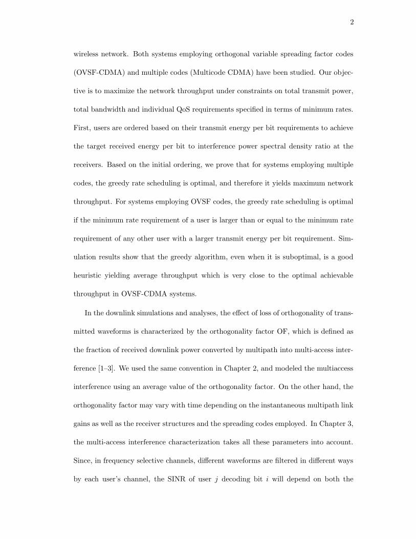
wireless network. Both systems employing orthogonal variable spreading factor codes

(OVSF-CDMA) and multiple codes (Multicode CDMA) have been studied. Our objec-

tive is to maximize the network throughput under constraints on total transmit power,

total bandwidth and individual QoS requirements specified in terms of minimum rates.

First, users are ordered based on their transmit energy per bit requirements to achieve





if the minimum rate requirement of a user is larger than or equal to the minimum rate

requirement of any other user with a larger transmit energy per bit requirement. Sim-

ulation results show that the greedy algorithm, even when it is suboptimal, is a good

heuristic yielding average throughput which is very close to the optimal achievable

throughput in OVSF-CDMA systems.

In the downlink simulations and analyses, the effect of loss of orthogonality of trans-

mitted waveforms is characterized by the orthogonality factor OF, which is defined as

the fraction of received downlink power converted by multipath into multi-access inter-

ference [1–3]. We used the same convention in Chapter 2, and modeled the multiaccess

interference using an average value of the orthogonality factor. On the other hand, the

orthogonality factor may vary with time depending on the instantaneous multipath link

gains as well as the receiver structures and the spreading codes employed. In Chapter 3,

the multi-access interference characterization takes all these parameters into account.

Since, in frequency selective channels, different waveforms are filtered in different ways

by each user’s channel, the SINR of user j decoding bit i will depend on both the

3

waveform si and the channel Hj . Therefore, it is crucial to determine which orthogonal

waveforms provide a given set of rate assignments. To this end, we study joint power

control and orthogonal code selection (rate control) in Chapter 3. We show that the

power control framework [4] can be extended to include rate control as well. Using

this framework, we prove that a joint power and rate control algorithm converges to

optimum assignments of multiaccess resources (time slots for TDMA, spreading codes

for CDMA, subcarriers for OFDM etc.) to users, and to optimum transmit power lev-

els such that the total transmit power is minimized while each transmitted bit can be

decoded with sufficient SINR. Specifically, for a CDMA wireless network, we observe

that the optimal solution is achieved when each user selects those spreading codes from

the Walsh set whose frequency domain responses match to the channel response of the

user.

Finally, in Chapter 4, we illustrate how to apply combinatorial network flow models

in wireless resource management problems. Network flows are well-known combinato-

rial subject with many applications in various fields of computer science, engineering,

management and operations research. The minimum cost flow problem, a fundamental

problem of network flows, deals with determining a least cost shipment of a commodity

through a network in order to satisfy demands at certain nodes from available supplies

at other nodes [5]. Here we model the communication through a wireless network as a

network flow and we aim to minimize the cost of information flow through the network

under constraints on demands (minimum rate) of mobiles and supply (bandwidth) of

the base station. This model helps us to deal with practical discrete system constraints,

and to improve fairness by enforcing minimum rate constraints on each mobile. We first

apply the network flow model in the case of an OFDM system where the channel is flat

4

on each subcarrier and frequency selective across the subcarriers. Next, we propose an

iterative minimum cost flow algorithm for CDMA networks and analyze its convergence

properties. Finally, we consider the downlink of a CDMA network with linear receiver

processing, and apply the network flow model in this system.

We summarize our work and give further research directions in Chapter 5.

5

Chapter 2

Optimum Rate Scheduling on the Downlink of a CDMA

Wireless Network

In this chapter, we investigate optimum rate scheduling on the downlink of a multirate

CDMA wireless network. Both systems employing orthogonal variable spreading factor

codes and multiple codes have been studied. Our objective is to maximize the network

throughput under constraints on total transmit power, total bandwidth, and individual

QoS requirements specified in terms of minimum rates.

The chapter starts with a brief background on the topic including the relevant

literature. In Section 2.2, we describe the system model and define the problem. The

optimum rate scheduling algorithms for both OVSF CDMA and Multicode CDMA

systems are discussed in Section 2.3, and the optimality of the proposed algorithms are

proven in Section 2.4. Examples and simulation results are given in Section 2.6. We

conclude the chapter with a brief summary and discussion.

2.1 Introduction

The multimedia oriented next generation wireless networks will provide multirate ser-

vices with various service classes in addition to classical voice service. In CDMA wireless

networks, multiple users share a common communication medium by means of spread-

ing codes. There are two ways to assign spreading codes in such systems. First, in

6

0,1 =(1)

C 1,1 =(1,1)

C 1,2 =(1,-1)

C 2,1 =(1,1,1,1)

C 2,2 =(1,1,-1,-1)

C 2,3 =(1,-1,1,-1)

C 2,4 =(1,-1,-1,1)

C 3,1

C 3,2

C 3,3

C 3,4

C 3,5

C 3,6

C 3,7

C 3,8

C

SF=1layer 1SF=2

layer 0 layer 2 SF=4

layer 3 SF=8

Rate=R Rate=R/2 Rate=R/4 Rate=R/8

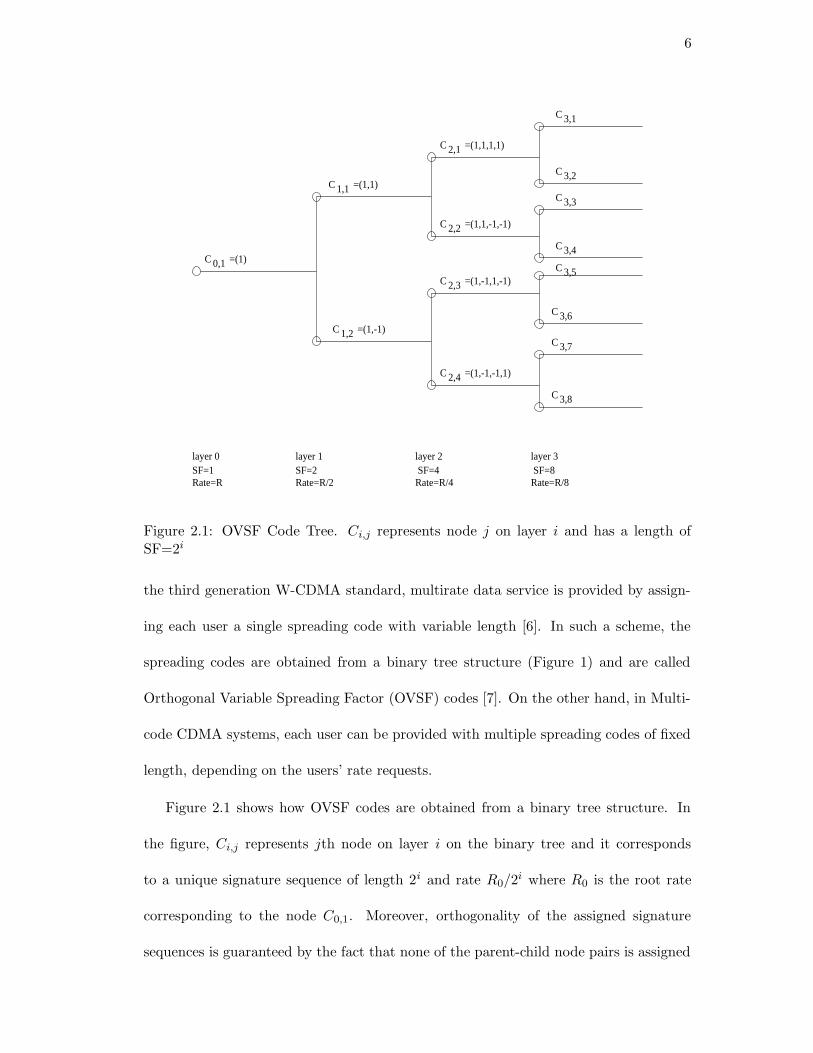
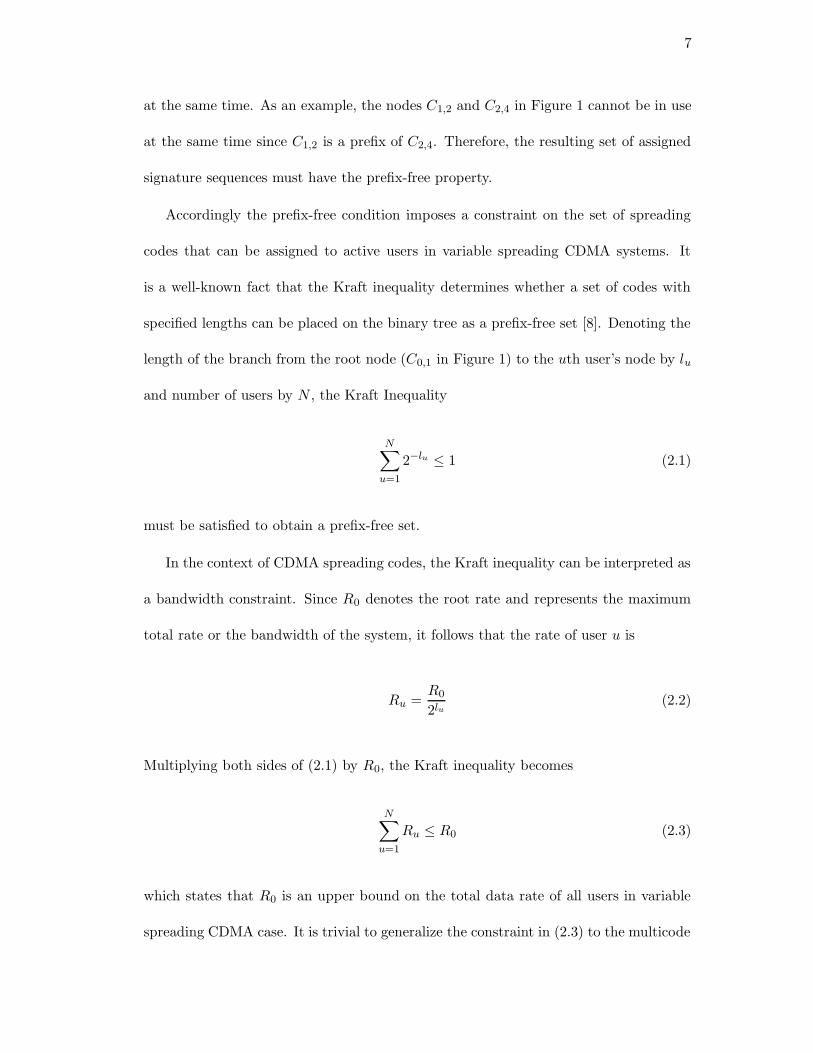
Figure 2.1: OVSF Code Tree. Ci,j represents node j on layer i and has a length ofSF=2i

the third generation W-CDMA standard, multirate data service is provided by assign-

ing each user a single spreading code with variable length [6]. In such a scheme, the

spreading codes are obtained from a binary tree structure (Figure 1) and are called

Orthogonal Variable Spreading Factor (OVSF) codes [7]. On the other hand, in Multi-

code CDMA systems, each user can be provided with multiple spreading codes of fixed

length, depending on the users’ rate requests.

Figure 2.1 shows how OVSF codes are obtained from a binary tree structure. In

the figure, Ci,j represents jth node on layer i on the binary tree and it corresponds

to a unique signature sequence of length 2i and rate R0/2i where R0 is the root rate

corresponding to the node C0,1. Moreover, orthogonality of the assigned signature

sequences is guaranteed by the fact that none of the parent-child node pairs is assigned

7

at the same time. As an example, the nodes C1,2 and C2,4 in Figure 1 cannot be in use

at the same time since C1,2 is a prefix of C2,4. Therefore, the resulting set of assigned

signature sequences must have the prefix-free property.

Accordingly the prefix-free condition imposes a constraint on the set of spreading

codes that can be assigned to active users in variable spreading CDMA systems. It

is a well-known fact that the Kraft inequality determines whether a set of codes with

specified lengths can be placed on the binary tree as a prefix-free set [8]. Denoting the

length of the branch from the root node (C0,1 in Figure 1) to the uth user’s node by lu

and number of users by N , the Kraft Inequality

N∑

u=1

2−lu ≤ 1 (2.1)

must be satisfied to obtain a prefix-free set.

In the context of CDMA spreading codes, the Kraft inequality can be interpreted as

a bandwidth constraint. Since R0 denotes the root rate and represents the maximum

total rate or the bandwidth of the system, it follows that the rate of user u is

Ru =R0

2lu(2.2)

Multiplying both sides of (2.1) by R0, the Kraft inequality becomes

N∑

u=1

Ru ≤ R0 (2.3)

which states that R0 is an upper bound on the total data rate of all users in variable

spreading CDMA case. It is trivial to generalize the constraint in (2.3) to the multicode

8

CDMA case and R0 represents the system bandwidth in this case.

Recent studies on multirate CDMA systems focus on efficiency of dynamic spreading

code assignment schemes, especially for systems employing OVSF codes [9–12]. The

basic question these studies attempt to answer is how to accommodate an incoming

user’s rate request on the OVSF code tree. For a multicode CDMA system it is easy

to handle an incoming user’s request, if the requested rate is within available network

resources, as many spreading codes as needed to meet the requested amount are as-

signed to the incoming user. On the other hand, in variable spreading CDMA systems

the inherent binary tree structure of OVSF codes complicates code management. For

example, assume there are 2 users in the system and their spreading codes are located

at C2,1 and C2,3 on the binary code tree in Figure 1. Thus the total used system band-

width is R/2 and half of the bandwidth is still available. In case a new user requests

R/2, the system cannot locate a spreading code for the new user since C1,1 (C1,2) is not

orthogonal to the existing code C2,3 (C2,1), although the system bandwidth is available

for this request. This is known as code blocking [9].

In [9, 11, 12], dynamic code assignment schemes are proposed to minimize the code

blocking probability and to minimize the number of existing spreading codes relocated

in case of an incoming user. In [10], the authors propose a protocol which uses a credit-

based reservation scheme to prioritize users and attempts to provide fairness to each

user while providing per-connection bandwidth guarantees to bursty data applications.

However, except for total available bandwidth, throughput limiting system resources

such as total transmit power is neglected in the above studies.

For the uplink of multirate CDMA systems, resource allocation problems are stud-

ied extensively in [13–22]. The common objective in these studies is either to maximize

9

the sum of rates (or utility), or to minimize the total transmit power, while there may

be constraints on individual transmit power assignments, total bandwidth, the quality

of reception in terms of SINR targets, minimum service requirement of each user (fair-

ness), or delay. In [13], both the problem of minimizing the total transmit power and

maximizing the sum of rates are considered. For the total power minimization problem,

a closed form solution in terms of a matrix equation is developed. For the throughput

maximization problem, a gradient projection algorithm is proposed, while its conver-

gence to a global optimum solution is not proved. In [14], throughput maximization

problem for a dual class CDMA system is considered. The objective in this study is

to maximize the throughput of delay tolerant users while minimizing the interference

caused by constant bit rate delay intolerant users. In [15], throughput is defined as the

sum of correctly received bits. Since there are no constraints on minimum rates in this

study, the optimum solution becomes unfair, allocating the whole bandwidth to the user

with the largest link gain. Processing gain selection and transmission power control for

multiple class CDMA networks are considered in [16–18]. The delay performances of

the proposed algorithms are also analyzed. Throughput maximization problems with

discrete set of rates are considered in [19, 20]. In [19], distributed control of rate and

power for the best effort data services is studied. The proposed greedy rate assign-

ment algorithm is claimed to maximize the number of users supported with minimum

rate in case of nonzero minimum rate requirements. Here we will show that, for the

downlink, the optimality of the greedy algorithm is in fact dependent on the minimum

rates in case of geometric set of rates, and the greedy rate scheduling is optimal only

if the minimum rate requirement of a user is larger than or equal to the minimum rate

requirement of any other user with a larger transmit energy per bit requirement to

10

achieve the target received SINR per bit at the receiver. Finally, CDMA power control

problems are analyzed in a game theoretic framework in [21, 22].

Since voice based networks, such as IS-95, provide real-time constant bit rate service

with QoS requirement in terms of target SINR at the base station, most of the initial

CDMA resource allocation research is focused on power control algorithms in the uplink

direction. On the other hand, multimedia oriented wireless networks provide data

services, such as web applications, wireless video etc., which require heavy traffic load

in the downlink direction. In [23–29], resource allocation problems for the downlink

CDMA systems are studied. A hierarchical SIR and rate control algorithm is proposed

in [23]. First, the mobiles determine their SIR targets using mobile specific information,

and then the base station determines rate assignments using the limited feedback from

the mobiles. Our analysis in this chapter will answer how the base station algorithm

in the hierarchical structure should work. Joint power control and intracell scheduling

for nonreal time data is studied in [24]. It is shown that a time division scheme in

which users transmit one by one fashion within each cell provides energy efficiency and

increased capacity. In [25], we study joint power control and orthogonal spreading code

selection in frequency selective multipath channels. We show that an iterative algorithm

achieves the optimal solution in which the total transmit power is minimized, while each

user selects the spreading codes from the Walsh set whose frequency domain responses

match to the channel response of the user. Finally, game theoretic pricing models are

applied for downlink CDMA systems in [26–29].

There are basic differences between the downlink and the uplink of CDMA systems.

First, orthogonal spreading codes are used in the downlink while random spreading

codes are used in the uplink. Thus, in a channel with no multipath, both the transmitted

11

and the received waveforms are orthogonal in the downlink direction. Second, both the

desired signal and the interferer signals go through the same channel in the downlink,

which means that both the interference powers and the desired signal power are filtered

equally by the mobile’s channel. We will explore these two important observations.

Using the orthogonality of the spreading codes, we model the overall system as a number

of parallel channels under the assumption of a flat channel. Using the same channel

argument, we are able to derive a closed form expression for the transmit energy per

bit requirement of each mobile to achieve the target SINR per bit at the receiver in

a frequency selective multipath channel. Once the transmit energy per bit targets are

determined, the problem formulation is simplified greatly as the interference constraints

are accounted for in the energy per bit expressions, and the problem formulation is the

same as that in the flat channel case.

Most of the literature on radio resource allocation assumes continuous rate and

power assignments, instead of realistic discrete system parameters, which simplifies

the problem at the expense of an approximate solution. Here, we assume practical

discrete rates corresponding to systems employing either multiple codes or variable

spreading codes (OVSF codes). In this case, the throughput maximization becomes a

discrete optimization problem. We show that for systems employing multiple codes,

the problem can be solved efficiently by a simple greedy algorithm with polynomial

complexity. Moreover, for systems employing variable spreading codes, we show that

the greedy algorithm is optimal if the minimum rate requirement of a user is larger than

or equal to the minimum rate requirement of any other user with worse channel quality1;

1By channel quality, we refer to the transmit energy per bit requirements to achieve the target SINRper bit at the receiver. Thus, a user with a smaller transmit energy per bit requirement is the userwith the better channel.

12

otherwise the greedy algorithm is only a heuristic yielding a suboptimal solution.

We note that the greedy algorithm in this chapter orders users based on transmit

energy per bit requirements which are shown to be not only a function of the path

loss, but also a function of other user specific parameters such as the orthogonality

factor, which is related to the multipath dispersion of the channel [1], and application

specific target received SINR per bit. Thus, an ordering by transmit energy per bit

requirements may not result in the same ordering as by path loss. We identify such

cases and show that, in short range wireless systems such as WLANs or Infostations

in which the average path loss is small compared to a cellular layout, the optimum

scheduling is based only on the orthogonality factor (multipath dispersion or multipath

delay profile) and the target received SINR per bit, and is independent of the path loss.

In the following section, we describe the system model, derive closed form expres-

sions for the transmit energy per bit requirements, and define the problem.

2.2 System Model and Problem Statement

We consider a single cell CDMA downlink. There are N active mobiles in the system.

Each mobile has a different application running and therefore each has a specific QoS

requirement in terms of a minimum service rate. For each transmitted bit of user u,

there is a target received energy per bit to interference power spectral density ratio,

or SINR per bit, denoted by (E/I)ru = γu, with which the receiver can decode the

transmitted bits with an acceptable bit error rate BER.

The channel between the base station and each mobile can be modeled either as a

frequency flat single path channel, or as a frequency selective multipath channel. These

two models have quite different implications on the problem definition. Since orthogonal

13

spreading codes are used on the downlink of the system, orthogonality of the transmitted

waveforms is preserved at each receiver under frequency flat channel assumption. On

the other hand, in a frequency selective multipath channel, the orthogonality of the

transmitted waveforms is lost at the receivers. Our problem definition will be general

enough to account for both channel models. We accomplish this by determining the

transmit energy per bit requirements for both channel models.

Since both the transmitted and the received waveforms are orthogonal in a fre-

quency flat channel, the overall system is modeled as a number of parallel channels,

and the question is how to assign rates on each parallel channel in the presence of total

transmit power and bandwidth (sum of rates) constraints at the base station. Since

there is no interference across parallel channels, the received E ru only compensates for

the background noise, i.e. (E/I)ru = (E/N0)

ru = γu, and therefore Er

u = γuN0 where

N0 is the noise power spectral density. In this case, the transmit energy per bit is given

by Etu = γuN0/hu where hu denotes the link gain for user u.

When there is multipath in the channel, delayed versions of orthogonal spreading

codes arrive at each receiver, leading to multi-access interference due to the loss of or-

thogonality between spreading codes. In the CDMA downlink, the effect of the loss of

orthogonality can be characterized by the orthogonality factor (OF), which is defined

as the fraction of received downlink power converted by multipath into multi-access in-

terference [1–3]. As noted in [1–3], the orthogonality factor is a time-varying parameter

that depends on the instantaneous multipath channels as well as the receiver structure

and the spreading codes employed. On the other hand, in the analysis of downlink, the

time average value of the orthogonality factor is traditionally employed [1–3]. Here we

follow the same convention, and assume that user u has an average orthogonality factor

14

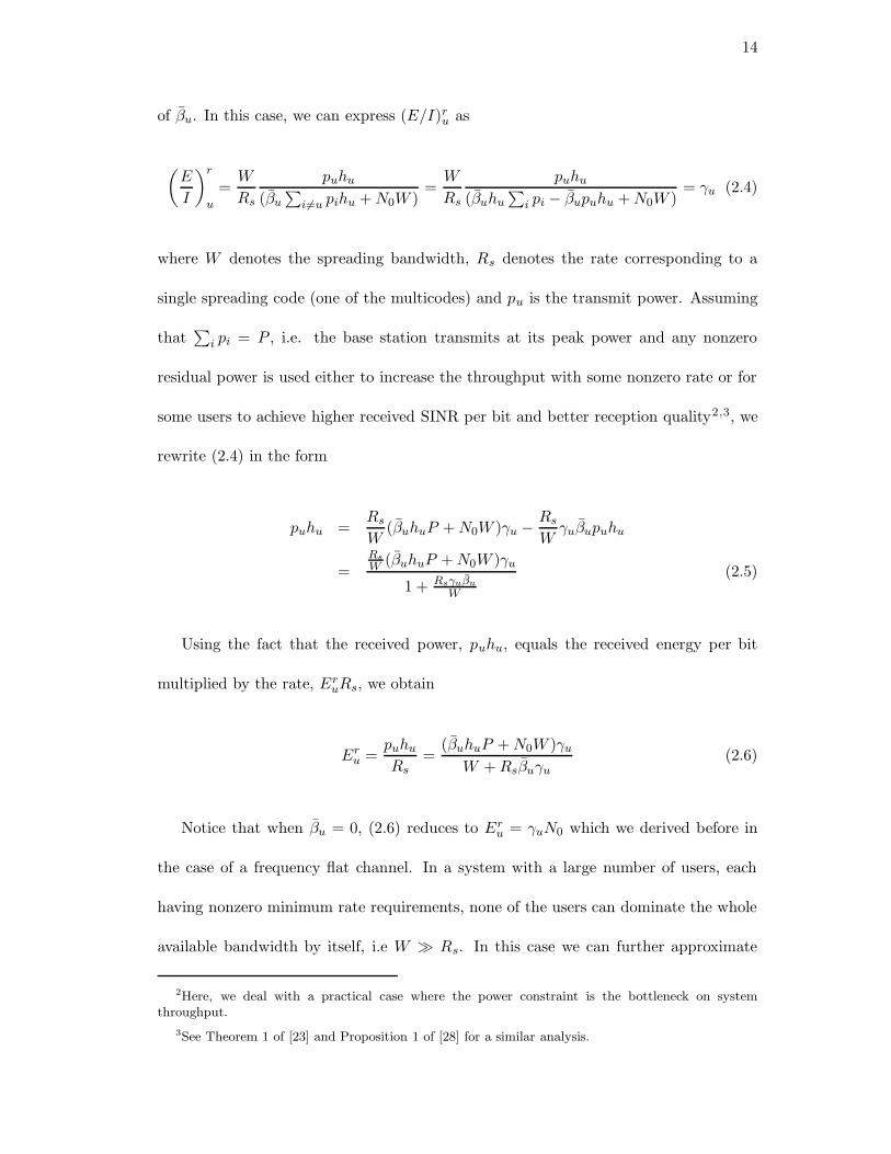
of βu. In this case, we can express (E/I)ru as

(

E

I

)r

u

=W

Rs

puhu

(βu

∑

i6=u pihu +N0W )=W

Rs

puhu

(βuhu

∑

i pi − βupuhu +N0W )= γu (2.4)

where W denotes the spreading bandwidth, Rs denotes the rate corresponding to a

single spreading code (one of the multicodes) and pu is the transmit power. Assuming

that∑

i pi = P , i.e. the base station transmits at its peak power and any nonzero

residual power is used either to increase the throughput with some nonzero rate or for

some users to achieve higher received SINR per bit and better reception quality2,3, we

rewrite (2.4) in the form

puhu =Rs

W(βuhuP +N0W )γu − Rs

Wγuβupuhu

=Rs

W(βuhuP +N0W )γu

1 + Rsγuβu

W

(2.5)

Using the fact that the received power, puhu, equals the received energy per bit

multiplied by the rate, EruRs, we obtain

Eru =

puhu

Rs=

(βuhuP +N0W )γu

W +Rsβuγu

(2.6)

Notice that when βu = 0, (2.6) reduces to Eru = γuN0 which we derived before in

the case of a frequency flat channel. In a system with a large number of users, each

having nonzero minimum rate requirements, none of the users can dominate the whole

available bandwidth by itself, i.e W � Rs. In this case we can further approximate

2Here, we deal with a practical case where the power constraint is the bottleneck on systemthroughput.

3See Theorem 1 of [23] and Proposition 1 of [28] for a similar analysis.

15

(2.6) as

Eru =

puhu

Rs≈ (βuhuP +N0W )γu

W(2.7)

A design based on (2.7) is more conservative than a design based on (2.6). While

the approximation is quite accurate for very low data rates, users with relatively high

rates achieve larger SINR per bit when constraint (2.7) is satisfied. Notice that E ru is

a decreasing function of Rs (2.6). Finally, the transmit energy per bit in the case of

a frequency selective channel is given by E tu = Er

u/hu. We note that Etu is required

for one of the multicodes corresponding to rate Rs. Assignment of multiple codes to a

user generates self interference. In this case, each spreading code needs to be treated

separately, and Etu has to be calculated for each of them as if every other spreading

code is an interferer signal.

An interesting observation is that when the received multiaccess interference power

is much larger than the receiver noise, i.e. βuhuP � N0W , the transmit energy per bit

becomes

Etu =

(βuhuP +N0W )γu

hu(W +Rsβuγu)≈ βuPγu

W +Rsβuγu

(2.8)

which is independent of the path loss. We will explore this fact in Section 2.5 to schedule

users in short range wireless systems such as WLANs or Infostations where the path

loss is small (hu is large) and the term βuhuP dominates N0W .

2.2.1 Problem Definition

We first examine OVSF CDMA systems. Given the minimum rate requirement of each

user and the constraint on the total BS power P , our problem is to assign each user

u a data rate Ru corresponding to a node on the OVSF code tree such that the Kraft

16

inequality (2.1), each user’s individual data rate and total BS power requirements are

satisfied and the total data rate of all users (network throughput) is maximized. The

problem in the multicode CDMA case is similar; given the minimum rate requirement

of each user and the constraint on the total BS power, we determine the number of

spreading codes that will be assigned to each user such that each user’s individual

data rate and total BS power requirements are satisfied and the network throughput is

maximized.

OVSF CDMA Rate Scheduling Problem

Let R0 denote the root rate, Ru and Ru,min denote the rate assignment and the mini-

mum rate requirement for user u respectively, and lu denote the length of the branch

from the root node (C0,1 in Figure 1) to the uth user’s node. Remember that there is a

one-to-one relationship between lu and Ru given by (2.2). In this case, R0 corresponds

to l0 = 0, and the minimum rate constraint Ru,min corresponds to maximum branch

length constraint lu ≤ lu,max = Lu. The problem is to find l=[l1, . . . , lN ] solving

maxl

N∑

u=1

R02−lu (2.9)

subject toN∑

u=1

EtuR02

−lu ≤ P (2.9a)

N∑

u=1

2−lu ≤ 1 (2.9b)

lu ∈ {0, 1, . . . , Lu} (2.9c)

In the above problem formulation, E tuR02

−lu is the transmit power for user u and (2.9a)

represents the total transmit power constraint. On the other hand, the Kraft inequality

17

(2.9b) is necessary to obtain a set of orthogonal codes, and represents the bandwidth

constraint.

Multicode CDMA Rate Scheduling Problem

The problem formulation for the multicode system is similar. Let Rs denote the rate

corresponding to a single spreading code, R0 denote the sum of rates of all spreading

codes, nu and Ru denote the number of spreading codes and the rate assignment for

user u respectively, thus Ru = Rsnu. Each user requires at least n′

u spreading codes as

the minimum QoS requirement. The problem is to find n=[n1, . . . , nN ] solving

maxn

N∑

u=1

Rsnu (2.10)

subject toN∑

u=1

EtuRsnu ≤ P (2.10a)

N∑

u=1

Rsnu ≤ R0 (2.10b)

nu ∈ {n′

u, n′

u + 1, . . . , R0/Rs} (2.10c)

2.3 Optimum Rate Scheduling Algorithms

Before the details of the algorithms, we first summarize our results. First, users are

ordered by their transmit energy per bit, E tu, requirements (from smallest to largest) in

order to achieve the target (E/I)ru = γu at the receivers. Based on the initial ordering:

1. For multicode systems, greedy rate scheduling is optimal, achieving maximum

network throughput.

2. For OVSF CDMA systems, greedy rate scheduling is optimal if the minimum rate

18

requirement of a user is larger than or equal to the minimum rate requirement

of any other user with a larger transmit energy per bit requirement, i.e. when

Eti < Et

j implies Li ≤ Lj for all i and j. 4

3. For OVSF CDMA systems in which minimum rates are not ordered by trans-

mit energy per bit requirements, the greedy rate scheduling achieves maximum

throughput if there is an optimal set of rate assignments ordering rates by the

transmit energy per bit requirements. Otherwise the greedy rate scheduling is

only a heuristic yielding a suboptimal solution.

We will show in the following sections that in cases where the greedy algorithm is

optimal, the set of rate assignments by any existing optimal algorithm can be made

more “greedy” by reordering and reassigning the user rates in a way to favor the users

with better channels. Moreover, as the rate assignments by the optimal algorithm look

more like the greedy assignments, the total power is reduced while keeping the total

throughput constant.

To see how reordering reduces the total power, assume N users with energy per

bit requirements Etb = [Et

1, Et2, . . . , E

tN ] and rate assignments R = [R1, R2, . . . , RN ]. If

Ri < Rj and Eti < Et

j , we can swap the rates of user i and j without changing the

total sum of rates, as long as the new assignments do not violate the minimum rate

constraints. Denoting the total transmit power before and after swapping Ri and Rj

4The statement includes the case where there is no minimum rate constraint on user rates, i.e.Lu = ∞ for all u, or all users have the same minimum rate constraint, i.e. Lu = L for all u.

19

Input : R0, P , £u = {0, 1, . . . , Lu}, Etb = [Et

1, Et2, . . . , E

tN ] (in increasing order)

Output : l=[l1, . . . , lN ]Initialization : lu = Lu, u = 1, . . . , NPt =

∑Nu=1 E

tuR02

−Lu

for u = 1 : Nlu = min{l ∈ £u| 2−l +

∑

v 6=u 2−lv ≤ 1, 2−l − 2−Lu ≤ P−Pt

EtuR0

}Pt = Pt +Et

uR0(2−lu − 2−Lu)

end

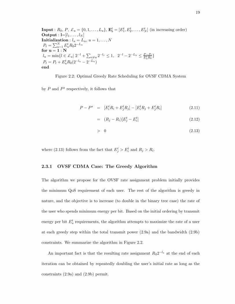
Figure 2.2: Optimal Greedy Rate Scheduling for OVSF CDMA System

by P and P s respectively, it follows that

P − P s = [EtiRi +Et

jRj] − [EtiRj +Et

jRi] (2.11)

= (Rj −Ri)[Etj −Et

i ] (2.12)

> 0 (2.13)

where (2.13) follows from the fact that E tj > Et

i and Rj > Ri.

2.3.1 OVSF CDMA Case: The Greedy Algorithm

The algorithm we propose for the OVSF rate assignment problem initially provides

the minimum QoS requirement of each user. The rest of the algorithm is greedy in

nature, and the objective is to increase (to double in the binary tree case) the rate of

the user who spends minimum energy per bit. Based on the initial ordering by transmit

energy per bit Etu requirements, the algorithm attempts to maximize the rate of a user

at each greedy step within the total transmit power (2.9a) and the bandwidth (2.9b)

constraints. We summarize the algorithm in Figure 2.2.

An important fact is that the resulting rate assignment R02−lu at the end of each

iteration can be obtained by repeatedly doubling the user’s initial rate as long as the

constraints (2.9a) and (2.9b) permit.

20

Notice that uth user’s spreading code resides on layer lu of the binary code tree in

Figure 2.1. Although lu uniquely determines the rate assignment for uth user (2.2),

it does not tell us which node on layer lu of the code tree should be assigned to user

u. On the other hand, satisfying the Kraft Inequality (2.1) guarantees the fact there

is at least a set of N spreading codes on the binary code tree such that uth user’s

spreading code is placed on layer lu, the rates of all other users are not affected by this

placement (although spreading codes might shift on the same layer) and all spreading

codes in the set are mutually orthogonal as a result of the prefix free property. The

shifts or replacements of spreading codes on the same layer on the binary code tree are

implementation issues and such shifts do not affect the assigned rate of a user. Thus,

the way the spreading code replacements or shifts occur at each step of the algorithms,

the subject of [9, 11] and [12], is not addressed in this study.

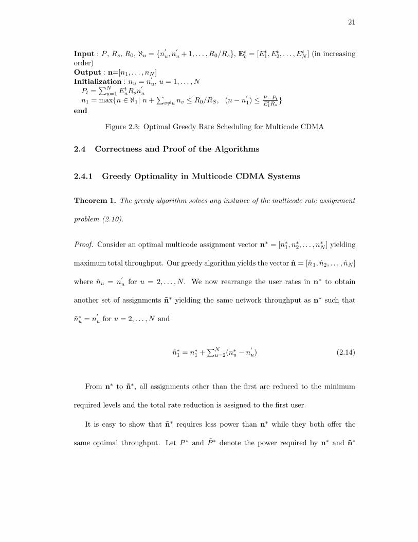
2.3.2 Multicode CDMA Case: The Greedy Algorithm

Similar to the OVSF system, the greedy approach solves the rate assignment problem

in multicode systems. However, in this case the greedy rate assignment only favors

the user with the smallest transmit energy per bit requirement. After the algorithm

assigns minimum rates and allocates corresponding spreading codes to each user, only

the rate of the user with the minimum energy per bit requirement is maximized using

the remaining power budget.

We summarize the algorithm above in Figure 2.3.

21

Input : P , Rs, R0, ℵu = {n′

u, n′

u + 1, . . . , R0/Rs}, Etb = [Et

1, Et2, . . . , E

tN ] (in increasing

order)Output : n=[n1, . . . , nN ]Initialization : nu = n

′

u, u = 1, . . . , NPt =

∑Nu=1E

tuRsn

′

u

n1 = max{n ∈ ℵ1| n+∑

v 6=u nv ≤ R0/RS , (n− n′

1) ≤ P−Pt

Et1Rs

}end

Figure 2.3: Optimal Greedy Rate Scheduling for Multicode CDMA

2.4 Correctness and Proof of the Algorithms

2.4.1 Greedy Optimality in Multicode CDMA Systems

Theorem 1. The greedy algorithm solves any instance of the multicode rate assignment

problem (2.10).

Proof. Consider an optimal multicode assignment vector n∗ = [n∗1, n∗2, . . . , n

∗N ] yielding

maximum total throughput. Our greedy algorithm yields the vector n = [n1, n2, . . . , nN ]

where nu = n′

u for u = 2, . . . , N . We now rearrange the user rates in n∗ to obtain

another set of assignments n∗ yielding the same network throughput as n∗ such that

n∗u = n′

u for u = 2, . . . , N and

n∗1 = n∗1 +∑N

u=2(n∗u − n

′

u) (2.14)

From n∗ to n∗, all assignments other than the first are reduced to the minimum

required levels and the total rate reduction is assigned to the first user.

It is easy to show that n∗ requires less power than n∗ while they both offer the

same optimal throughput. Let P ∗ and P ∗ denote the power required by n∗ and n∗

22

respectively, then

P ∗ − P ∗ = Et1Rs(n

∗1 − n∗1) +

N∑

u=2

EtuRs(n

∗u − n∗u)

≥ Et1Rs[(n

∗1 − n∗1) +

N∑

u=2

(n∗u − n∗u)]

= 0 (2.15)

The last inequality follows from the fact that user 1 requires the smallest energy per

bit, and replacing Etu by Et

1 upperbounds P ∗ − P ∗ since (n∗u − n∗u) ≥ 0.

Comparing n∗ and the greedy n, they agree on all rate assignments except the first

user. On the other hand, for mobile 1, the greedy algorithm makes a locally maximum

choice and maximizes its rate within power and bandwidth constraints, while assuming

that all other users receive the minimum rates. Therefore n1 ≥ n∗1. On the other hand,

since n∗ obtains maximum total throughput by assumption, n∗1 ≥ n1. We conclude

that n∗1 = n1 and n∗ = n.

The intuition behind the optimality of the greedy algorithm is that if a spreading

code is to be assigned, it is better if it is assigned to the user who can receive it with

the smallest power (the smallest contribution to the total power). On the other hand,

unlike uplink where the multiaccess interference at the receiver depends on the channels

of all users and the individual power assignments, the multiaccess interference on the

downlink is a function of the user’s own channel and the power assignments of interferer

spreading codes. Thus, a reduction in the power of any interferer signal is beneficial to

all users no matter who the spreading code is assigned to.

23

2.4.2 Greedy Optimality in OVSF CDMA Systems

We first prove the optimality of the greedy algorithm in the two user case. We then

generalize the proof to any number of users.

Theorem 2. Given that the user with smaller transmit energy per bit requirement has

also larger (or equal) minimum rate requirement, the greedy algorithm solves the OVSF

rate assignment problem for N = 2 users.

Proof. A general form of the problem in the 2 user case is as follows

max R0(2−l1 + 2−l2) (2.16)

subject to Et1R02

−l1 +Et2R02

−l2 ≤ P′

(2.16a)

2−l1 + 2−l2 ≤ ρ (2.16b)

li ∈ {0, 1, . . . , Li}, i = 1, 2 (2.16c)

for any 0 < P′ ≤ P and 0 < ρ ≤ 1. Assume that the first user requires smaller transmit

energy per bit Et1 < Et

2.

Consider an optimal vector l∗ = [l∗1, l∗2] yielding maximum total throughput. Given

L1 ≤ L2, we can always choose the optimal vector l∗ in such a way that l∗1 ≤ l∗2;

otherwise if L1 ≤ L2 and l∗1 > l∗2, user 1 and user 2 can exchange the assigned values so

that the total throughput remains the same and the new assignments even save some

power. Note that such an exchange may violate individual minimum rate constraints

24

if L1 > L2. Our greedy algorithm yields the vector l = [l1, l2]

l1 = min{l ∈ £|2−l + 2−L2 ≤ ρ, Et1R02

−l +Et2R02

−L2 ≤ P′} (2.17)

l2 = min{l ∈ £|2−l + 2−l1 ≤ ρ, Et2R02

−l +Et1R02

−l1 ≤ P′} (2.18)

We compare l∗ and l

(i) Assume l∗1 < l1 : For user 1, the greedy algorithm finds the minimum layer num-

ber l1 while power and bandwidth constraints are satisfied and second user’s spreading

code resides on layer L2. Thus l∗1 < l1 is impossible; otherwise l1 would not be the local

minimum choice.

(ii) Assume l∗1 > l1 : In this case the smallest possible value of l∗1 is l1 + 1. Since

l∗1 ≤ l∗2, we have

l1 + 1 ≤ l∗1 ≤ l∗2 (2.19)

Since l∗ is optimal, it must offer the maximum total throughput. This requires

R0(2−l1 + 2−l2) ≤ R0(2

−l∗1 + 2−l∗

2 ) (2.20)

However, from (2.19),

R0(2−l∗

1 + 2−l∗2 ) ≤ R0(2

−(l1+1) + 2−(l1+1)) = R02−l1 < R0(2

−l1 + 2−l2) (2.21)

since 0 ≤ l2 ≤ L2. Thus we have a contradiction implying l∗1 > l1 is also impossible. As

a result we conclude that l∗1 = l1.

Similar to user 1, the greedy algorithm makes a local minimum choice for user 2

25

while the first user’s spreading code resides on layer l1. Because l∗1 = l1, and l2 is a

local minimum, l2 ≤ l∗2 must be true. On the other hand if l2 < l∗2, then the optimal l∗

offers smaller throughput compared to the greedy l, which is a contradiction. Therefore

l∗2 = l2 must be true. Since we also proved that l∗1 = l1, we conclude l∗ = l.

We next generalize the proof to any number of users.

Theorem 3. Given that minimum rate requirement of a user is larger than or equal

to minimum rate requirement of any other user with a larger transmit energy per bit

requirement, the greedy algorithm solves the OVSF rate assignment problem.

Proof. Here we will prove a more general statement that the greedy algorithm solves

rate maximization problem for any power constraint 0 < P′ ≤ P and any bandwidth

constraint 0 < ρ ≤ 1, corresponding to a “partial” binary code tree. The general form

of the problem is

max

N∑

u=1

R02−lu (2.22)

subject to

N∑

u=1

EtuR02

−lu ≤ P′ ≤ P (2.22a)

N∑

u=1

2−lu ≤ ρ ≤ 1 (2.22b)

lu ∈ {0, 1, . . . , Lu} (2.22c)

Without loss of generality, we can assume that E t1 < Et

2 < · · · < EtN . Consider

an optimal vector l∗ = [l∗1, l∗2, . . . , l

∗N ] yielding maximum total throughput. Given L1 ≤

L2 ≤ · · · ≤ LN , any set of optimal rate assignments can be reordered in such a way

that l∗1 ≤ l∗2 ≤ · · · ≤ l∗N , without violating individual minimum rate constraints. It is

26

important to notice that, given E ti < Et

j and l∗i > l∗j , an exchange between assignments

of users i and j does not violate minimum rate constraints if Li ≤ Lj5. Note that

such an ordering always saves power (2.11)-(2.13), therefore the power constraint is

not violated while the throughput remains constant. Our greedy algorithm yields the

vector l = [l1, l2, . . . , lN ].

The proof goes by induction. We already proved the greedy optimality for the two

user case in Theorem 2. Here, we assume that Theorem 3 is true for any system of

N < N users. We also assume that there is a feasible rate assignment vector for the

problem (2.22). Therefore, optimal and greedy solutions are both feasible and we will

consider them below.

Definition 1. Let A be a user index such that

lu = l∗u u = 1, . . . , A− 1 (2.23)

lA 6= l∗A

Due to local optimality of the greedy algorithm, (2.23) can be made more specific

lA ≤ l∗A − 1 (2.24)

First of all we assume A > 1. In this case at least the first user gets the same rate

assignment by both algorithms (greedy and optimal). The remaining N − 1 users can

be assigned in a greedy fashion because our induction hypothesis stipulates that for

5In fact, the proof is valid as long as there exists an optimal algorithm whose output rate assignmentscan be reordered in such a way that E

ti < E

tj implies li ≤ lj , without violating individual minimum

rate constraints.

27

any N < N users, greedy assignments are optimal. This proves Theorem 3 for the case

of A > 1. Thus, it remains to consider the case of A = 1. Since optimal l∗ achieves

maximum total throughput, employing (2.24) for the case A = 1 we can write that

2−l∗1 +

N∑

u=2

2−l∗u ≥ 2−(l∗1−1) +

N∑

u=2

2−Lu (2.25)

Lemma 1. For any l∗ = [l∗1, l∗2, . . . , l

∗N ] satisfying (2.25), we can always find a set of

assignments l∗2, . . . , l∗N such that

2−l∗1 +

N∑

u=2

2−l∗u = 2−(l∗1−1) +

N∑

u=2

2−l∗u (2.26)

l∗u ≤ l∗u ≤ Lu, u = 2, . . . , N (2.27)

Proof of Lemma 1. Here we give a constructive proof of Lemma 1 by providing an

explicit algorithm which computes the new assignments l∗2, . . . , l∗N . The algorithm is

presented in Figure 2.4. In the figure, n, 4n and Jn denote iteration index, bandwidth

released by decreasing rate of a user at nth iteration and the aggregate bandwidth

released up to the nth iteration respectively.

We will show by contradiction that the aggregate bandwidth released Jn equals to

2−l∗1 at some point, and that the algorithm falls through Step 3 and always terminates.

Let’s assume that there is no n such that Jn = 2−l∗1 . Together with (2.25) it means

that there will be such an iteration t for which

Jt−1 < 2−l∗1 (2.28)

Jt > 2−l∗1

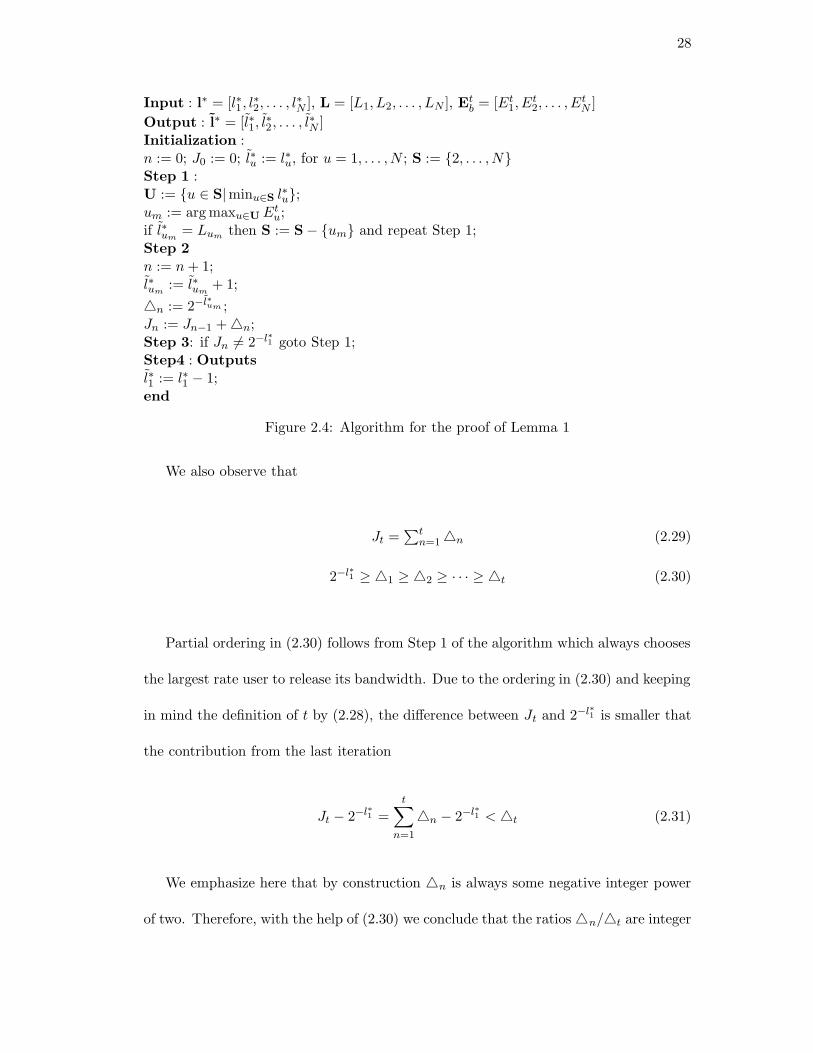
28

Input : l∗ = [l∗1, l∗2, . . . , l

∗N ], L = [L1, L2, . . . , LN ], Et

b = [Et1, E

t2, . . . , E

tN ]

Output : l∗ = [l∗1, l∗2, . . . , l

∗N ]

Initialization :n := 0; J0 := 0; l∗u := l∗u, for u = 1, . . . , N ; S := {2, . . . , N}Step 1 :U := {u ∈ S|minu∈S l

∗u};

um := arg maxu∈U Etu;

if l∗um= Lum

then S := S− {um} and repeat Step 1;Step 2n := n+ 1;l∗um

:= l∗um+ 1;

4n := 2−l∗um ;Jn := Jn−1 + 4n;Step 3: if Jn 6= 2−l∗

1 goto Step 1;Step4 : Outputsl∗1 := l∗1 − 1;end

Figure 2.4: Algorithm for the proof of Lemma 1

We also observe that

Jt =∑t

n=1 4n (2.29)

2−l∗1 ≥ 41 ≥ 42 ≥ · · · ≥ 4t (2.30)

Partial ordering in (2.30) follows from Step 1 of the algorithm which always chooses

the largest rate user to release its bandwidth. Due to the ordering in (2.30) and keeping

in mind the definition of t by (2.28), the difference between Jt and 2−l∗1 is smaller that

the contribution from the last iteration

Jt − 2−l∗1 =

t∑

n=1

4n − 2−l∗1 < 4t (2.31)

We emphasize here that by construction 4n is always some negative integer power

of two. Therefore, with the help of (2.30) we conclude that the ratios 4n/4t are integer

29

numbers for n = 1, . . . , t. Next, we divide both sides of (2.31) by 4t

(

t∑

n=1

4n

4t

)

− 2−l∗1

4t< 1 (2.32)

In the above inequality, the left side is a positive integer due to (2.28), while the

right side is a fractional number less than one. Therefore (2.32) contains a contradiction,

proving that Step 3 terminates the algorithm which results in the set of assignments

l∗2, . . . , l∗N as in Lemma 1.

With the help of Lemma 1, we can immediately construct a new rate assignment

vector l∗ = [l∗1 − 1, l∗2 , . . . , l∗N ] yielding the same throughput as the optimal assignments

l∗, yet because of (2.27), it consumes less energy. Notice that l∗ looks more “greedy”

than l∗, i.e. user 1 with the minimum transmit energy per bit requirement gets an

enhanced rate while the other users get less than or equal to their rate assignments in

l∗ due to (2.27).

To complete the proof of Theorem 3 in the case of A = 1, Lemma 1 can be applied

to l∗ as well, i.e. starting from the new set of optimal assignments l∗, we can construct

another optimal set with the first user receiving l∗1 − 2 and all other users receive less

than or equal to their assignments in l∗, but more than their minimum requirements.

We can continue in this fashion until the first user receives l1, the assignment by the

greedy algorithm, in an optimal set of assignments. At this point, we already proved the

greedy optimality, i.e. for A > 1 using our induction hypothesis that greedy assignments

are optimal for any N < N users. The greedy optimality proof of Theorem 2 in the

two user case is therefore generalized to any number of users by induction.

30

2.4.3 Discussion

It is interesting to note that the optimality of the greedy algorithm in OVSF CDMA

systems depends on the minimum rate constraints. When users with worse channels

require larger minimum rates, the greedy algorithm may not be the optimal way to

assign user rates. As a simple example, assume there are two users in the system; the

first with Et1 = 1, and the second one with Et

2 = 1.25 (for simplicity, we omit the units

and assume all units are consistent and scaled appropriately). The power constraint is

11, and minimum rate requirements are R1,min = 1 and R2,min = 4. Total power to

provide the minimum rates is

Pmin =2∑

u=1

EtuRu,min = 6 (2.33)

Since the first user requires smaller transmit energy per bit, the greedy algorithm

would double (note the geometric relationship between rates on the binary code tree)

the first user’s initial rate assignment using the remaining power budget of 11 − 6 = 5.

In this case, the greedy algorithm could at most assign 4 units of rate to user one, which

requires an additional 3 units of power. The remaining 11 − 6 − 3 = 2 units of power

would not be enough to double second user’s initial assignment from 4 to 8, therefore

the greedy algorithm would conclude R1 = 4, R2 = 4 and a total throughput of 8 units

of rate. On the other hand, optimal throughput is 9 units of rate which is achieved when

R1 = 1 and R2 = 8. In this case, optimal transmission strategy is to favor the user with

the worse channel, which contradicts with the opportunistic transmission strategies in

which users with better channels are favored.

We note that discrete optimization problems, or integer programming problems,

31

are in general NP-complete so that they cannot be solved by simple algorithms with

polynomial complexity such as greedy algorithms. One such intractable problem, which

is similar to the throughput maximization problem, is the Knapsack problem in which

one wish to fill a knapsack of capacity b with items having the largest possible total

utility [30, 31]. Formally,

max

n∑

j=1

cjxj (2.34)

subject ton∑

j=1

ajxj ≤ b (2.34a)

xj integers, 0-1 or 0 ≤ xj ≤ 1 (2.34b)

where cj, aj and xj denote the utility, the size/capacity and the amount included in

the knapsack for jth item respectively. Similarly in resource allocation problems, the

power constraint represents the knapsack capacity, and the target is to achieve the

largest total utility by filling the knapsack by as much rate (item) as possible. Based

on constraints on xj, the Knapsack problems are classified either as integer knapsack

problems, where xj is constrained to be positive integers, 0 − 1 knapsack problems,

where xj is constrained to be 0 or 1 only, or fractional knapsack problems where xj

may be a fractional number and we may take pieces of items [32]. While the integer

knapsack and the 0 − 1 knapsack problems are NP-complete, the fractional knapsack

problems can be solved by greedy algorithms with polynomial complexity [32]. There

is a sizeable theory behind the knapsack problems and we will not go into its details

here. Instead, we conjecture that those OVSF CDMA problems which are not greedy

solvable are NP complete due to similar reasons for NP completeness of some Knapsack

problems.

32

2.5 Examples and Simulations

We apply the algorithms on the downlink of a single cell CDMA wireless network. The

system assumptions are consistent with 3G system specifications. Spreading gain is

assumed to be in the range from a minimum of 4 upto 512, which corresponds to 8

levels on the binary code tree including the root node. The spreading bandwidth is

3.84 MHz, maximum base station transmission power is 10 Watts, the receiver noise,

NoW , is 10−13 Watts, and the target (E/I)ru = γu is 5 (7dB) (different applications

may have different γu targets, the algorithms are applicable in such cases as well). The

x any y coordinates of each mobile are selected uniformly on (0-2000m) in a square cell

of 4km2. The path loss at any given distance d is given by [33]

PL = A+ 10ε log10(d/d0) + s; d ≥ d0 (2.35)

where A is the decibel path loss at distance d0, ε is the path loss exponent, and s is the

shadow fading variation. The numerical values are d0=100 m, A=78 dB, s is lognormal

with σ=8 dB, and ε=4. The multipath characteristics, or the frequency selectivity, of

the channels are represented by the orthogonality factor β; for simplicity we assume

that all users have the same average β. The experiments are conducted for β = 0, which

corresponds to a flat channel, β = 0.1, β = 0.5 and β = 0.8. Each mobile requires a

minimum rate corresponding to one of {128, 256, 512} length spreading codes with equal

probability. We assume fixed modulation and coding 6.

6There is no explicit assumption on modulation and coding format. The only assumption is thatthey are the same and fixed for all users, which implies that spreading codes with the same lengthscorrespond to the same rate, and the rate assignments are proportional to the number of spreadingcode assignments. In numerical calculations, we assumed uncoded QPSK, while the algorithms andanalysis are valid for any fixed coding and modulation format.

33

0 5 10 15 20 25 30 350

0.1

0.2

0.3

0.4

0.5

0.6

0.7

0.8

0.9

1

number of users

ave

rag

e t

hro

ug

hp

ut

− s

cale

d t

o t

he

fla

t/m

ulti

cod

e t

hro

ug

hp

ut

beta=0, greedy MCbeta=0, greedy OVSFbeta=0.1, greedy MCbeta=0.1, greedy OVSFbeta=0.5, greedy MCbeta=0.5, greedy OVSFbeta=0.8, greedy MCbeta=0.8, greedy OVSF

beta=0.8

beta=0.5

beta=0.1,beta=0

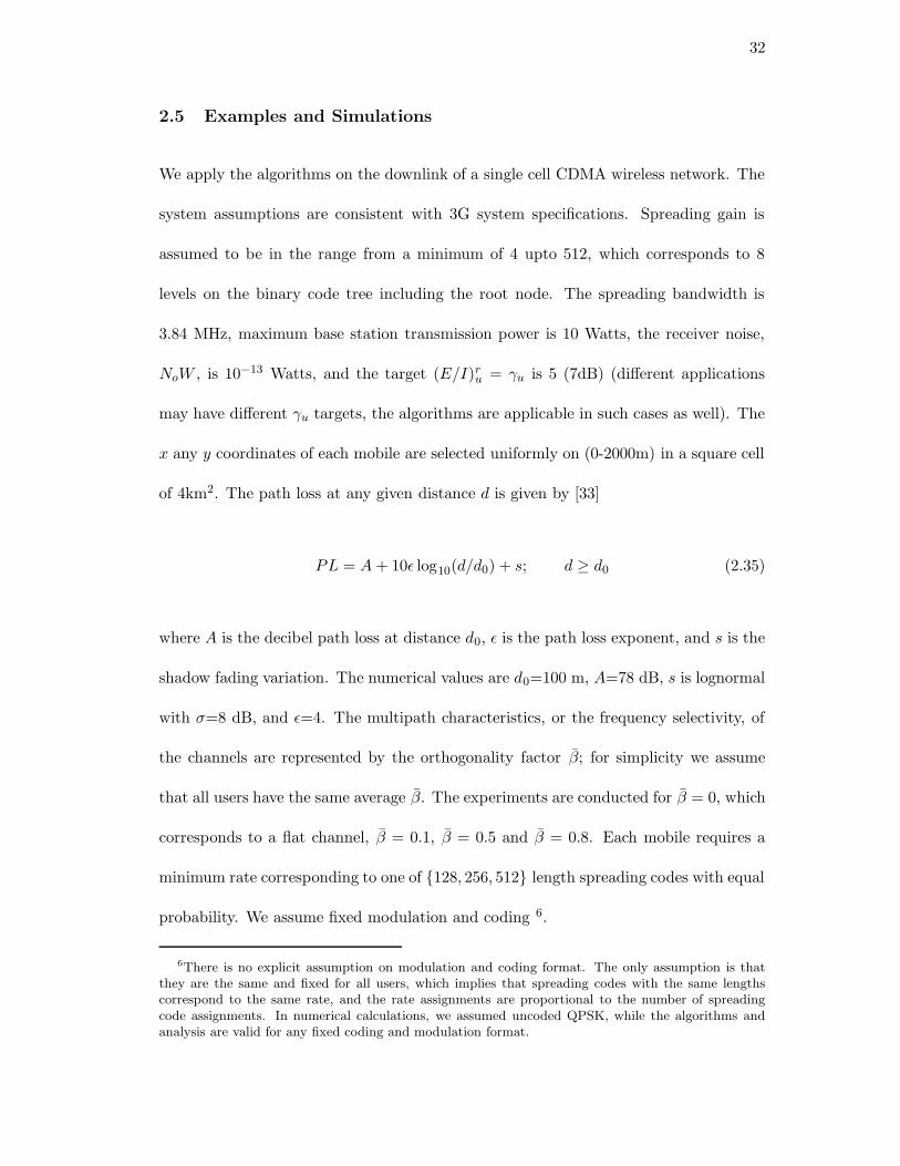
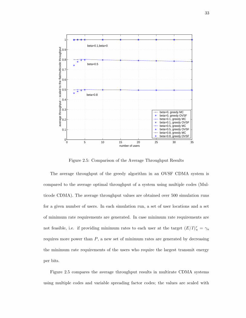
Figure 2.5: Comparison of the Average Throughput Results

The average throughput of the greedy algorithm in an OVSF CDMA system is

compared to the average optimal throughput of a system using multiple codes (Mul-

ticode CDMA). The average throughput values are obtained over 500 simulation runs

for a given number of users. In each simulation run, a set of user locations and a set

of minimum rate requirements are generated. In case minimum rate requirements are

not feasible, i.e. if providing minimum rates to each user at the target (E/I)ru = γu

requires more power than P , a new set of minimum rates are generated by decreasing

the minimum rate requirements of the users who require the largest transmit energy

per bits.

Figure 2.5 compares the average throughput results in multirate CDMA systems

using multiple codes and variable spreading factor codes; the values are scaled with

34

Path Loss (dB) 71 78 93 97 107 108 110 124 127 129

Ru,min (Kbps) 15 60 15 15 15 15 15 60 15 60

Ru (Kbps), β = 0 960 480 240 60 15 15 15 60 15 60

Ru (Kbps), β = 0.1 960 480 240 60 15 15 15 60 15 60

Ru (Kbps), β = 0.5 960 240 120 30 15 15 15 60 15 60

Ru (Kbps), β = 0.8 480 240 30 30 15 15 15 60 15 60

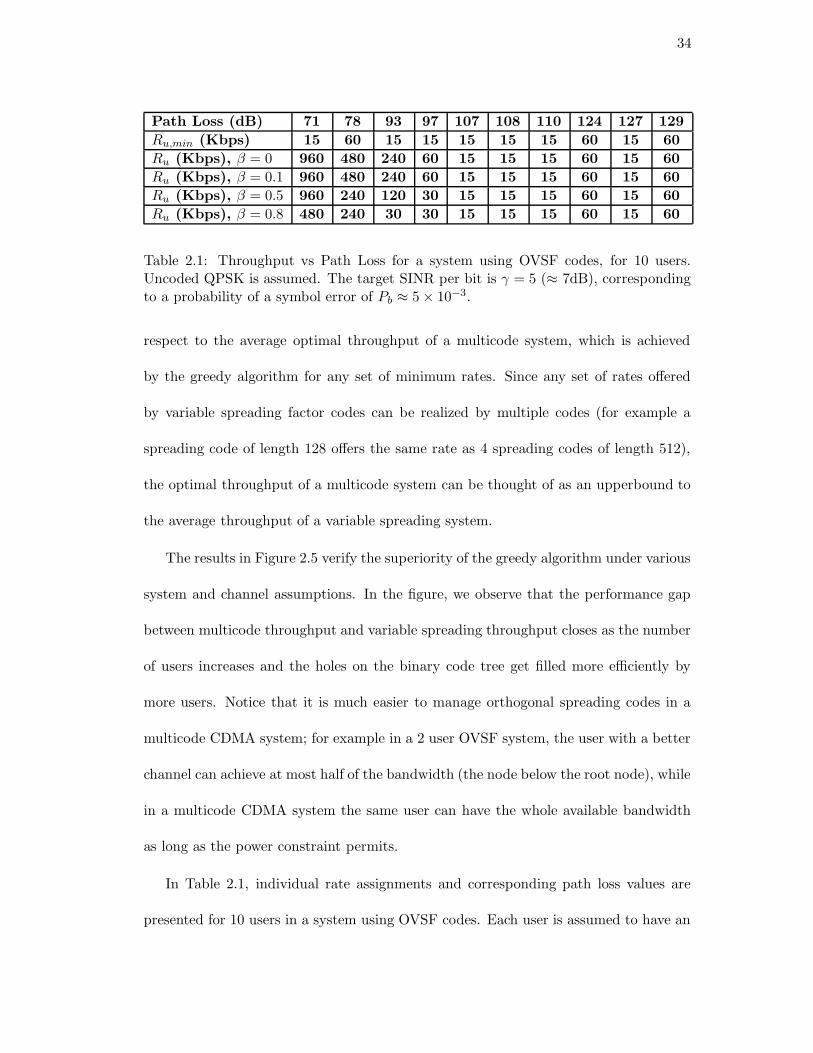
Table 2.1: Throughput vs Path Loss for a system using OVSF codes, for 10 users.Uncoded QPSK is assumed. The target SINR per bit is γ = 5 (≈ 7dB), correspondingto a probability of a symbol error of Pb ≈ 5 × 10−3.

respect to the average optimal throughput of a multicode system, which is achieved

by the greedy algorithm for any set of minimum rates. Since any set of rates offered

by variable spreading factor codes can be realized by multiple codes (for example a

spreading code of length 128 offers the same rate as 4 spreading codes of length 512),

the optimal throughput of a multicode system can be thought of as an upperbound to

the average throughput of a variable spreading system.

The results in Figure 2.5 verify the superiority of the greedy algorithm under various

system and channel assumptions. In the figure, we observe that the performance gap

between multicode throughput and variable spreading throughput closes as the number

of users increases and the holes on the binary code tree get filled more efficiently by

more users. Notice that it is much easier to manage orthogonal spreading codes in a

multicode CDMA system; for example in a 2 user OVSF system, the user with a better

channel can achieve at most half of the bandwidth (the node below the root node), while

in a multicode CDMA system the same user can have the whole available bandwidth

as long as the power constraint permits.

In Table 2.1, individual rate assignments and corresponding path loss values are

presented for 10 users in a system using OVSF codes. Each user is assumed to have an

35

Path Loss (dB) 10 20 30 40 50 60 70 80 90 100

OF (β) 0.7 0.4 0.3 0.2 0.1 0.1 0.1 0.1 0.1 0.1

Ru,min (Kbps) 15 15 15 15 15 15 15 15 15 15

Ru (Kbps) 15 15 15 15 960 480 240 60 15 15

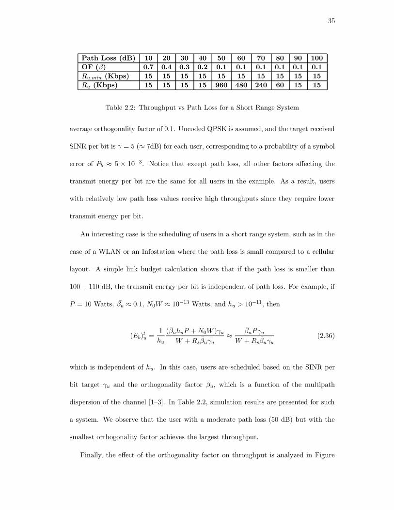
Table 2.2: Throughput vs Path Loss for a Short Range System

average orthogonality factor of 0.1. Uncoded QPSK is assumed, and the target received

SINR per bit is γ = 5 (≈ 7dB) for each user, corresponding to a probability of a symbol

error of Pb ≈ 5 × 10−3. Notice that except path loss, all other factors affecting the

transmit energy per bit are the same for all users in the example. As a result, users

with relatively low path loss values receive high throughputs since they require lower

transmit energy per bit.

An interesting case is the scheduling of users in a short range system, such as in the

case of a WLAN or an Infostation where the path loss is small compared to a cellular

layout. A simple link budget calculation shows that if the path loss is smaller than

100 − 110 dB, the transmit energy per bit is independent of path loss. For example, if

P = 10 Watts, βu ≈ 0.1, N0W ≈ 10−13 Watts, and hu > 10−11, then

(Eb)tu =

1

hu

(βuhuP +N0W )γu

W +Rsβuγu

≈ βuPγu

W +Rsβuγu

(2.36)

which is independent of hu. In this case, users are scheduled based on the SINR per

bit target γu and the orthogonality factor βu, which is a function of the multipath

dispersion of the channel [1–3]. In Table 2.2, simulation results are presented for such

a system. We observe that the user with a moderate path loss (50 dB) but with the

smallest orthogonality factor achieves the largest throughput.

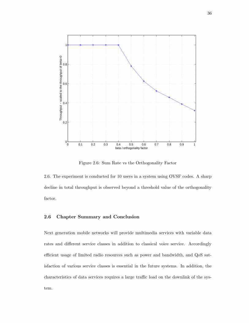
Finally, the effect of the orthogonality factor on throughput is analyzed in Figure

36

0 0.1 0.2 0.3 0.4 0.5 0.6 0.7 0.8 0.9 10

0.2

0.4

0.6

0.8

1

beta / orthogonality factor

Th

rou

gh

pu

t −

sca

led

to

th

e t

hro

ug

hp

ut

of

be

ta=

0

Figure 2.6: Sum Rate vs the Orthogonality Factor

2.6. The experiment is conducted for 10 users in a system using OVSF codes. A sharp

decline in total throughput is observed beyond a threshold value of the orthogonality

factor.

2.6 Chapter Summary and Conclusion

Next generation mobile networks will provide multimedia services with variable data

rates and different service classes in addition to classical voice service. Accordingly

efficient usage of limited radio resources such as power and bandwidth, and QoS sat-

isfaction of various service classes is essential in the future systems. In addition, the

characteristics of data services requires a large traffic load on the downlink of the sys-

tem.

37

In this chapter, we investigated throughput maximization on the downlink of a

CDMA wireless network. Both systems employing orthogonal variable spreading factor

codes (OVSF CDMA) and multiple codes (multicode CDMA) have been studied. The

objective is to maximize the network throughput under constraints on total transmit

power, total bandwidth and individual QoS requirements specified in terms of minimum

rates. First, users are ordered based on transmit energy per bit requirements to achieve





if the minimum rate requirement of a user is larger than or equal to the minimum

rate requirement of any other user with a larger transmit energy per bit requirement.

Simulation results show that the greedy algorithm, even when it is suboptimal, is a

good heuristic yielding average throughput which is very close to the optimal achievable

throughput in OVSF CDMA systems. The simplicity and polynomial time complexity

of the greedy algorithms seem to be very attractive from an implementation point of

view.

38

Chapter 3

Joint Power and Rate Control in Multiaccess Systems

with Multirate Services

In this chapter, we study joint power and rate control for wireless multiaccess systems

providing multirate services in a frequency selective multipath channel. We show that

the power control framework [4] can be extended to include rate control as well. Using

this framework, we prove that a joint power and rate control algorithm converges to

optimum assignments of multiaccess resources (time slots for TDMA, spreading codes

for CDMA, subcarriers for OFDM etc.) to users, and to optimum transmit power

levels such that the total transmit power is minimized while each transmitted bit can

be decoded with sufficient signal to interference plus noise ratio (SINR).

The chapter starts with a brief background on the topic including the relevant litera-

ture. In Section 3.2, we describe the system model and define the problem. An iterative

algorithm is proposed in Section 3.3, and its convergence properties are analyzed in the

same section. In Section 3.4, we apply the proposed algorithm on the downlink of a

multirate CDMA wireless network. We conclude the chapter with a brief summary and

discussion.

39

3.1 Introduction

In wireless multiaccess systems, multiple users share a common communication medium.

In TDMA systems, the medium is shared via time slots. In CDMA systems, spreading

codes provide users access to the communication medium. Similarly, for an OFDM

system, a number of subcarriers provide access to the common medium. While multiple

user’s information bits are transmitted simultaneously in one way or another, each user

has to achieve a level of quality of service (QoS) within system constraints such as total

transmit power or bandwidth.

Since wireless resources are scarce and expensive, a careful and efficient allocation is

vital. For example, in CDMA based IS-95 systems, power control is a useful technique

to regulate transmit powers of constant bit rate voice users so as to minimize the effect

of multiaccess interference (see [34] for a survey on this topic).

On the other hand, current and future wireless networks such as 3G cellular, WLANs

or 4G wireless networks, are based on supporting multirate data services such as multi-

media applications, internet access etc., in addition to classical voice service. For data

service, users may employ multiple time slots or multiple spreading codes, and may

receive variable rates. In this case, efficient resource allocation requires optimization

and control of multiple parameters simultaneously, such as joint control of transmit

power and rate assignments.

In the context of CDMA systems, combined power and rate control algorithms have

been studied in [35–37]. Two algorithms have been proposed in [35], one is based on

Lagrangian relaxation techniques and the other, called selective power control, is an

extension of a fixed rate power control algorithm. On the other hand, the basic idea

40

in [36, 37] is to adapt (reduce) the rate when the transmit power required to achieve a

target QoS exceeds a threshold. For multirate CDMA systems, the uplink throughput

maximization problem has been formulated in [13–15]. For the networks with multiple

service classes, the authors aim to satisfy different QoS requirements while utilizing the

system resources in an efficient way.

Since voice based networks, such as IS-95, provide real-time constant bit rate service

with QoS requirement in terms of target SINR at the base station, most of the initial

CDMA resource allocation research is focused on power control algorithms in the uplink

direction. On the other hand, multimedia oriented wireless networks provide multirate

data services, such as web applications, wireless video etc., which require heavy traffic

load in the downlink direction. Our focus in this chapter is the downlink power and

rate allocation.

In Chapter 2, the downlink throughput maximization problem is considered, where

the effect of loss of orthogonality of transmitted waveforms is characterized by the or-

thogonality factor. Using the orthogonality factor simplifies the problem formulation

considerably since, with a single variable, we account for the combined effects of spread-

ing codes employed, receiver structures and instantaneous multipath channel coefficients

on the multiaccess interference. The main motivation in this chapter is to exploit the

effects of all these parameters on the system performance, which are implicitly ne-

glected by using the orthogonality factor. The rationale is that, unlike uplink where

random spreading codes are used, fixed and deterministic Walsh codes1 are used on the

downlink. On the other hand, in frequency selective channels, different waveforms are

1Although CDMA networks are emphasized throughout the chapter, the analyses are valid for anymulti-access scheme using orthogonal waveforms on the downlink.

41

filtered in different ways by each user’s channel so that the SINR of user j decoding bit

i will depend on both the waveform si and the channel Hj . Therefore, it is crucial to

determine which orthogonal waveforms provide a given set of rate assignments.


We consider multirate data transmission on the downlink of a single cell multiaccess

system. There are K users in the cell. A multiaccess system is represented by a set of

N orthogonal unit energy waveforms denoted by S(t) = {s1(t), s2(t), . . . , sN (t)}. Each

waveform in S(t) is zero outside the transmission interval [0, T ]. For a TDMA system

{si(t) = ψ(t − (i − 1)T/N), i = 1, . . . , N} where ψ(t) is a square pulse on the interval

[0, T/N ]. For a CDMA system {si(t) =∑N

j=1 sijψ(t−(j−1)T/N), i = 1, . . . , N} where

ψ(t) is the chip waveform nonzero in the interval [0, T/N ] and sij =∫ T

0 si(t)ψ(t− (j −

1)T/N)dt. In the case of an OFDM system, N OFDM tones or subcarriers may be

viewed as the waveform set.

Projecting time signals onto an appropriate basis in each multiaccess system, we

obtain vector representation of the waveform set, S = {s1, s2, . . . , sN} where si ∈ CN .

In each tranmission interval [0, T ], base station transmits N waveforms in S. Multirate

transmission is provided by assigning multiple waveforms to a user. A waveform si is

transmitted with power pi and is assigned to a user j such that user j can reliably

decode (achieves target SINR γ) si using filter cij .

Each bit is denoted by bi, thus the base station transmits the signal

x =N∑

i=1

√pibisi (3.1)

42

1jh

1jh

1jh

3jh

3jh

1jh

1jh

1jh

3jh

3jh1-jNh

1-jNh

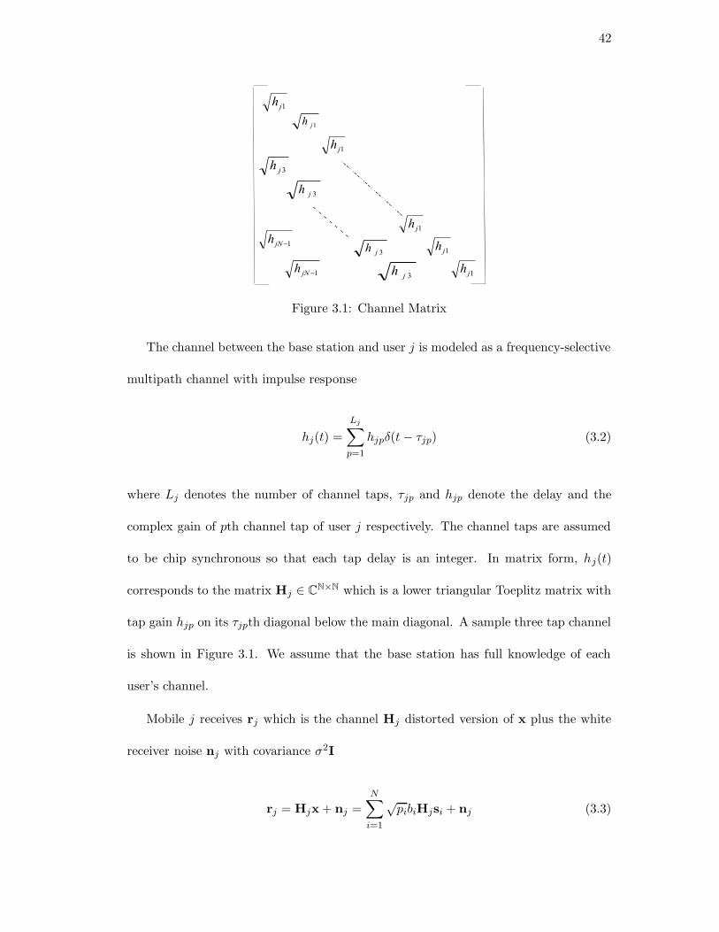
Figure 3.1: Channel Matrix

The channel between the base station and user j is modeled as a frequency-selective

multipath channel with impulse response

hj(t) =

Lj∑

p=1

hjpδ(t− τjp) (3.2)

where Lj denotes the number of channel taps, τjp and hjp denote the delay and the

complex gain of pth channel tap of user j respectively. The channel taps are assumed

to be chip synchronous so that each tap delay is an integer. In matrix form, hj(t)

corresponds to the matrix Hj ∈ CN×N which is a lower triangular Toeplitz matrix with

tap gain hjp on its τjpth diagonal below the main diagonal. A sample three tap channel

is shown in Figure 3.1. We assume that the base station has full knowledge of each

user’s channel.

Mobile j receives rj which is the channel Hj distorted version of x plus the white

receiver noise nj with covariance σ2I

rj = Hjx + nj =

N∑

i=1

√pibiHjsi + nj (3.3)

43

There is no predetermined or fixed assignment of waveforms to users and the base

station has to decide which waveform should be assigned to which user. This is a crucial

point in our problem formulation. Since the channels are frequency-selective, different

waveforms get distorted in a different ways by each user’s channel. Therefore the SINR

of user j decoding bit i will depend on both the waveform si and the channel Hj.

To decode its own bit or bits, mobile j passes the received signal rj through a bank

of receiver filters, one for each waveform si. Denoting the noise power at the output of

a filter by σ2, the signal to noise plus interference ratio γi achieved at the output of the

filter cij is

γi =pi(c

TijHjsi)

2

∑

v 6=i pv(cTijHjsv)2 + σ2(cT

ijcij)(3.4)

Our problem is to minimize the total power required to transmit N waveforms to

K users where N may or may not be equal to K. For each waveform si, we will decide

on a user j intended to receive si, a receiver filter cij , and a transmit power pi required

to achieve the target SINR γ while user j decodes its transmitted bit on the waveform

si. Note that the number of waveforms assigned to a user determines the rate assigned

to that user.

The optimization problem is as follows

min

N∑

i=1

pi (3.5)

s.t. maxj

maxcij

(

pi(cTijHjsi)

2

∑

v 6=i pv(cTijHjsv)2 + σ2(cT

ijcij)

)

≥ γ (3.5b)

pi ≥ 0, cij ∈ CN , i = 1, . . . , N

44

The constraint in (3.5b) guarantees that for a given waveform si, there is at least

one user j∗ ∈ {1, . . . ,K} and a receiver filter cij∗ that can decode si with acceptable

quality.

3.3 Solution

Similar power minimization problems have been well studied in literature [4, 38]. Our

problem definition adds user selection into the formulation. In each transmission inter-

val, the base station has to determine how many waveforms each user will be assigned

to, and accordingly how may bits each user will receive. From this point of view, (3.5)

may be viewed as a joint power and rate control problem.

We follow a similar analysis to that in [38]. We rewrite (3.5) in the form of a

standard power control problem [4].

min

N∑

i=1

pi (3.6)

s.t. pi ≥ minj

mincij

(

γ(∑

v 6=i pv(cTijHjsv)

2 + σ2(cTijcij))

(cTijHjsi)2

)

pi ≥ 0, cij ∈ CN , i = 1, . . . , N

We define

p = [p1, . . . , pN ] (3.7)

Ii(p, j, cij) =γ(∑

v 6=i pv(cTij

Hjsv)2+σ2(cTij

cij))

(cTij

Hjsi)2(3.8)

45

In the context of [4], the interference function I(p) becomes

I(p) = [I1(p), . . . , IN (p)] (3.9)

where

Ii(p) = minj

mincij

Ii(p, j, cij) (3.10)

We propose the following iterative algorithm

p(n+ 1) = I(p(n)) (3.11)

The framework of [4] tells us that an iterative algorithm in the form of (3.11) con-

verges to the minimum power solution if the interference function I(p) is standard [4].

Next, we will show that I(p) is standard. Therefore, when the algorithm (3.11)

converges, we obtain 1) optimum matchings (si, j) between waveforms and the users,

2) optimum receiver filter cij that user j will use to decode si, 3) optimum power

assignments p = [p1, . . . , pN ] that minimizes the objective function in (3.5).

Theorem 1. I(p) = [I1(p), . . . , IN (p)] is a standard interference function.

Proof. In order I(p) to be standard, it has to satisfy Positivity, Monotonicity and

Scalability properties, see [4] for details about these properties.

The positivity property is straightforward. For any user position j and filter cij ,

Ii(p) is always positive for any p ≥ 0 since Ii(p, j, cij) in (3.8) contains only summation,

multiplication and division of positive terms.

Monotonicity is satisfied if p ≥ p′implies I(p) ≥ I(p

′). From (3.8), for any given

j and cij , p ≥ p′implies Ii(p, j, cij) ≥ Ii(p

′, j, cij). Notice that increasing each power

46

assignment from p′

i to pi results in a larger sum in the numerator of (3.8). Assume the

arguments satisfying the equality Ii(p) = minj mincijIi(p, j, cij) occurs at j∗ and c∗ij

then

Ii(p) = minj mincijIi(p, j, cij) (3.12)

= Ii(p, j∗, c∗ij) (3.13)

≥ Ii(p′, j∗, c∗ij) (3.14)

≥ mincijIi(p

′, j∗, cij) (3.15)

≥ minj mincijIi(p

′, j, cij) = Ii(p

′) (3.16)

Scalability is satisfied if α > 1 implies αI(p) > I(αp). From (3.8), for any given j

and cij , α > 1 implies αIi(p, j, cij) > Ii(αp, j, cij). Notice that multiplying the whole

expression in (3.8) with α > 1 results in multiplication of the nonnegative background

noise σ2 with α as well, thus αIi(p, j, cij) > Ii(αp, j, cij) follows. To show scalability

αIi(p) = minj mincijαIi(p, j, cij) (3.17)

= αIi(p, j∗, c∗ij) (3.18)

> Ii(αp, j∗, c∗ij) (3.19)

> mincijIi(αp, j

∗, cij) (3.20)

> minj mincijIi(αp, j, cij ) = Ii(αp) (3.21)

Since I(p) satisfies positivity, monotonicity and scalability properties, I(p) is a standard

interference function.

47

Theorem 2. The solution of minj mincijIi(p, j, cij) occurs at j∗ and cij∗ where

Ai,k =

N∑

v 6=i

pv(Hksv)(Hksv)T + σ2I (3.22)

j∗ = arg mink∈{1,...,K}

((Hksi)T A−1

i,k (Hksi))−1 (3.23)

cij∗ =

√pi

1 + pi(Hj∗si)TA−1ij∗(Hj∗si)

A−1i,j∗Hj∗si (3.24)

Proof. We rewrite (3.8) as

Ii(p, j, cij) =γ cT

ij(∑N

v 6=i pv(Hjsv)(Hjsv)T + σ2I)cij

(cTijHjsi)2

(3.25)

For a given p and j, cij that minimizes (3.25) maximizes the left side of (3.5b),

which is the SINR achieved at the output of cij . Therefore cij must be the SINR

maximizing MMSE filter [38, 39] which is given as

cij =

√pi

1 + pi(Hjsi)TA−1ij (Hjsi)

A−1ij Hjsi (3.26)

where

Aij =N∑

v 6=i

pv(Hjsv)(Hjsv)T + σ2I (3.27)

For a given user j and its MMSE filter cij (3.26), the value of Ii(p, j, cij) becomes

γ ((Hjsi)TA−1

ij Hjsi)−1 (3.28)

In this case, j∗ ∈ {1, . . . ,K} that minimizes (3.28) and its corresponding MMSE

filter cij∗ (3.26) is the solution of minj mincijIi(p, j, cij).

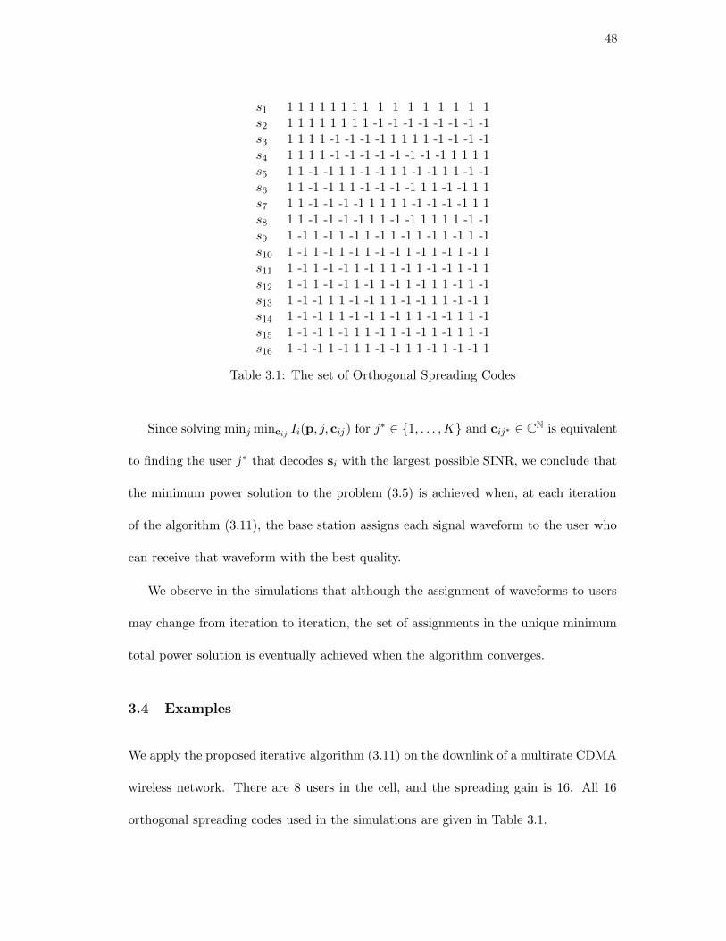
48

s1 1 1 1 1 1 1 1 1 1 1 1 1 1 1 1 1s2 1 1 1 1 1 1 1 1 -1 -1 -1 -1 -1 -1 -1 -1s3 1 1 1 1 -1 -1 -1 -1 1 1 1 1 -1 -1 -1 -1s4 1 1 1 1 -1 -1 -1 -1 -1 -1 -1 -1 1 1 1 1s5 1 1 -1 -1 1 1 -1 -1 1 1 -1 -1 1 1 -1 -1s6 1 1 -1 -1 1 1 -1 -1 -1 -1 1 1 -1 -1 1 1s7 1 1 -1 -1 -1 -1 1 1 1 1 -1 -1 -1 -1 1 1s8 1 1 -1 -1 -1 -1 1 1 -1 -1 1 1 1 1 -1 -1s9 1 -1 1 -1 1 -1 1 -1 1 -1 1 -1 1 -1 1 -1s10 1 -1 1 -1 1 -1 1 -1 -1 1 -1 1 -1 1 -1 1s11 1 -1 1 -1 -1 1 -1 1 1 -1 1 -1 -1 1 -1 1s12 1 -1 1 -1 -1 1 -1 1 -1 1 -1 1 1 -1 1 -1s13 1 -1 -1 1 1 -1 -1 1 1 -1 -1 1 1 -1 -1 1s14 1 -1 -1 1 1 -1 -1 1 -1 1 1 -1 -1 1 1 -1s15 1 -1 -1 1 -1 1 1 -1 1 -1 -1 1 -1 1 1 -1s16 1 -1 -1 1 -1 1 1 -1 -1 1 1 -1 1 -1 -1 1

Table 3.1: The set of Orthogonal Spreading Codes

Since solving minj mincijIi(p, j, cij) for j∗ ∈ {1, . . . ,K} and cij∗ ∈ C

N is equivalent

to finding the user j∗ that decodes si with the largest possible SINR, we conclude that

the minimum power solution to the problem (3.5) is achieved when, at each iteration

of the algorithm (3.11), the base station assigns each signal waveform to the user who

can receive that waveform with the best quality.

We observe in the simulations that although the assignment of waveforms to users

may change from iteration to iteration, the set of assignments in the unique minimum

total power solution is eventually achieved when the algorithm converges.

3.4 Examples

We apply the proposed iterative algorithm (3.11) on the downlink of a multirate CDMA

wireless network. There are 8 users in the cell, and the spreading gain is 16. All 16

orthogonal spreading codes used in the simulations are given in Table 3.1.

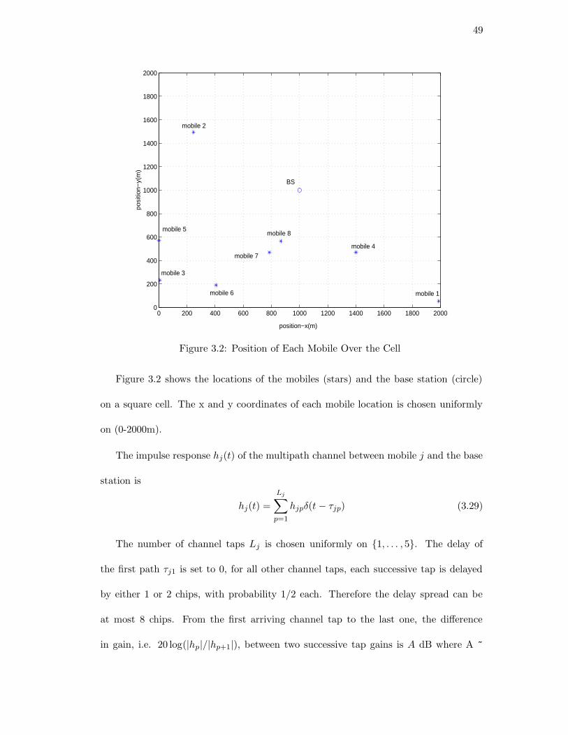
49

0 200 400 600 800 1000 1200 1400 1600 1800 20000

200

400

600

800

1000

1200

1400

1600

1800

2000

position−x(m)

po

sitio

n−

y(m

)

mobile 1

mobile 2

mobile 3

mobile 4

mobile 5

mobile 6

mobile 7

mobile 8

BS

Figure 3.2: Position of Each Mobile Over the Cell

Figure 3.2 shows the locations of the mobiles (stars) and the base station (circle)

on a square cell. The x and y coordinates of each mobile location is chosen uniformly

on (0-2000m).

The impulse response hj(t) of the multipath channel between mobile j and the base

station is

hj(t) =

Lj∑

p=1

hjpδ(t− τjp) (3.29)

The number of channel taps Lj is chosen uniformly on {1, . . . , 5}. The delay of

the first path τj1 is set to 0, for all other channel taps, each successive tap is delayed

by either 1 or 2 chips, with probability 1/2 each. Therefore the delay spread can be

at most 8 chips. From the first arriving channel tap to the last one, the difference

in gain, i.e. 20 log(|hp|/|hp+1|), between two successive tap gains is A dB where A ~

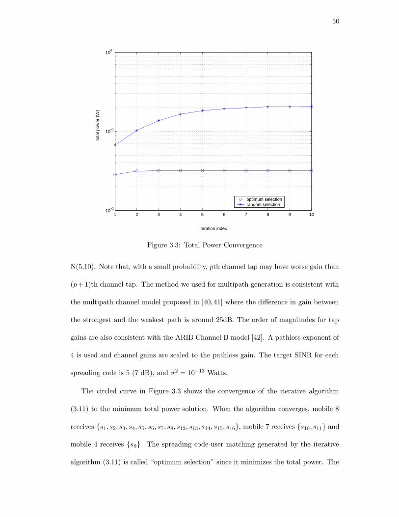
50

1 2 3 4 5 6 7 8 9 1010

−2

10−1

100

tota

l pow

er (

W)

iteration index

optimum selectionrandom selection

Figure 3.3: Total Power Convergence

N(5,10). Note that, with a small probability, pth channel tap may have worse gain than

(p+1)th channel tap. The method we used for multipath generation is consistent with

the multipath channel model proposed in [40, 41] where the difference in gain between

the strongest and the weakest path is around 25dB. The order of magnitudes for tap

gains are also consistent with the ARIB Channel B model [42]. A pathloss exponent of

4 is used and channel gains are scaled to the pathloss gain. The target SINR for each

spreading code is 5 (7 dB), and σ2 = 10−13 Watts.

The circled curve in Figure 3.3 shows the convergence of the iterative algorithm

(3.11) to the minimum total power solution. When the algorithm converges, mobile 8

receives {s1, s2, s3, s4, s5, s6, s7, s8, s12, s13, s14, s15, s16}, mobile 7 receives {s10, s11} and

mobile 4 receives {s9}. The spreading code-user matching generated by the iterative

algorithm (3.11) is called “optimum selection” since it minimizes the total power. The

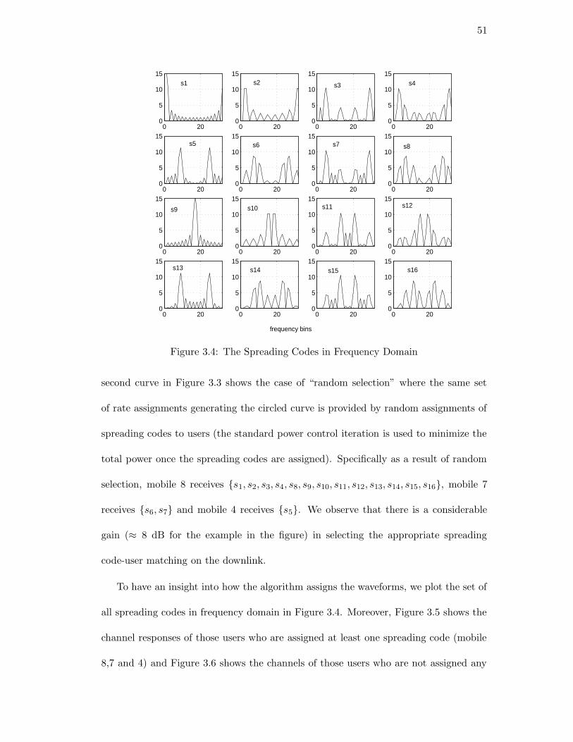
51

0 200

5

10

15

0 200

5

10

15

0 200

5

10

15

0 200

5

10

15

0 200

5

10

15

0 200

5

10

15

0 200

5

10

15

0 200

5

10

15

0 200

5

10

15

0 200

5

10

15

0 200

5

10

15

0 200

5

10

15

0 200

5

10

15

0 200

5

10

15

0 200

5

10

15

0 200

5

10

15

s1 s2 s3 s4

s5 s6 s7 s8

s9 s10 s11 s12

s13 s14 s15 s16

frequency bins

Figure 3.4: The Spreading Codes in Frequency Domain

second curve in Figure 3.3 shows the case of “random selection” where the same set

of rate assignments generating the circled curve is provided by random assignments of

spreading codes to users (the standard power control iteration is used to minimize the

total power once the spreading codes are assigned). Specifically as a result of random

selection, mobile 8 receives {s1, s2, s3, s4, s8, s9, s10, s11, s12, s13, s14, s15, s16}, mobile 7

receives {s6, s7} and mobile 4 receives {s5}. We observe that there is a considerable

gain (≈ 8 dB for the example in the figure) in selecting the appropriate spreading

code-user matching on the downlink.

To have an insight into how the algorithm assigns the waveforms, we plot the set of

all spreading codes in frequency domain in Figure 3.4. Moreover, Figure 3.5 shows the

channel responses of those users who are assigned at least one spreading code (mobile

8,7 and 4) and Figure 3.6 shows the channels of those users who are not assigned any

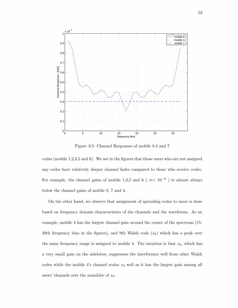
52

0 5 10 15 20 25 300

0.1

0.2

0.3

0.4

0.5

0.6

0.7

0.8

0.9

1x 10

−5

frequency bins

Cha

nnel

Res

pons

e −

|H(f

)|

mobile 8mobile 4mobile 7

Figure 3.5: Channel Responses of mobile 8,4 and 7

codes (mobile 1,2,3,5 and 6). We see in the figures that those users who are not assigned

any codes have relatively deeper channel fades compared to those who receive codes.

For example, the channel gains of mobile 1,3,5 and 6 ( ≈< 10−6 ) is almost always

below the channel gains of mobile 8, 7 and 4.

On the other hand, we observe that assignment of spreading codes to users is done

based on frequency domain characteristics of the channels and the waveforms. As an

example, mobile 4 has the largest channel gain around the center of the spectrum (15-

20th frequency bins in the figures), and 9th Walsh code (s9) which has a peak over

the same frequency range is assigned to mobile 4. The intuition is that s9, which has

a very small gain on the sidelobes, suppresses the interference well from other Walsh

codes while the mobile 4’s channel scales s9 well as it has the largest gain among all

users’ channels over the mainlobe of s9.

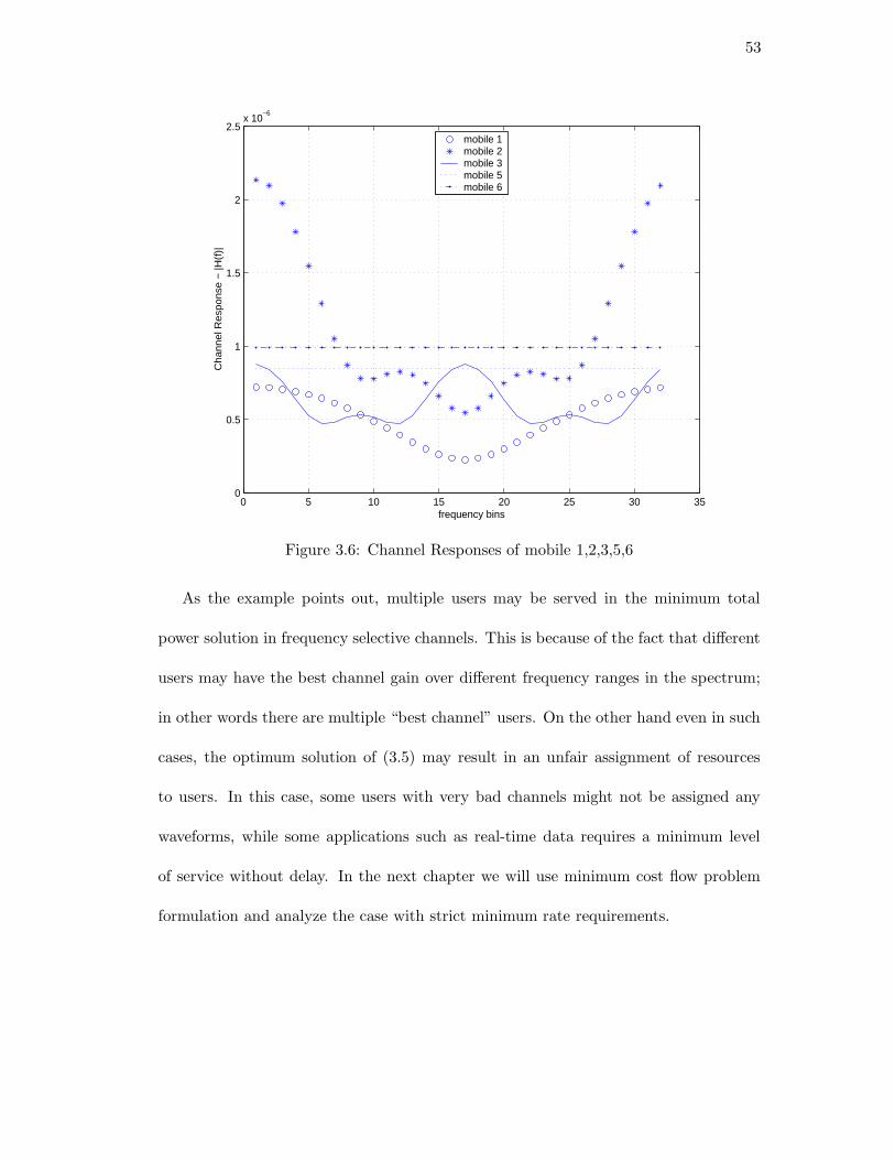
53

0 5 10 15 20 25 30 350

0.5

1

1.5

2

2.5x 10

−6

frequency bins

Cha

nnel

Res

pons

e −

|H(f

)|

mobile 1mobile 2mobile 3mobile 5mobile 6

Figure 3.6: Channel Responses of mobile 1,2,3,5,6

As the example points out, multiple users may be served in the minimum total

power solution in frequency selective channels. This is because of the fact that different

users may have the best channel gain over different frequency ranges in the spectrum;

in other words there are multiple “best channel” users. On the other hand even in such

cases, the optimum solution of (3.5) may result in an unfair assignment of resources

to users. In this case, some users with very bad channels might not be assigned any

waveforms, while some applications such as real-time data requires a minimum level

of service without delay. In the next chapter we will use minimum cost flow problem

formulation and analyze the case with strict minimum rate requirements.

54


In this chapter, we examined joint power control and orthogonal code selection (rate

control) for wireless multiaccess systems providing multirate services in frequency se-

lective multipath channels. We proposed an iterative algorithm converging to optimum

assignments of multiaccess resources to users, and to optimum transmit power levels

such that the total transmit power is minimized while each transmitted bit can be de-

coded with sufficient signal to interference plus noise ratio (SINR). Simulation results

for CDMA networks show that there is a considerable gain (≈ 8 dB for the particular

example in the text) in selecting the appropriate spreading code-user matching on the

downlink.

55

Chapter 4

Minimum Cost Network Flows and Strict Rate

Requirements

Network flows are well-known combinatorial subject with many applications in vari-

ous fields of computer science, engineering, management and operations research. The

minimum cost flow problem, a fundamental problem of network flows, deals with de-

termining a least cost shipment of a commodity through a network in order to satisfy

demands at certain nodes from available supplies at other nodes [5]. Here we model the

communication through a wireless network as a network flow and we aim to minimize

the cost of information flow through the network under constraints on demands (min-

imum rate) of mobiles and supply (bandwidth) of the base station. This model helps

us to improve fairness by enforcing minimum rate constraints on each mobile.

The chapter starts with a brief background on the topic including the relevant

literature. In Section 4.2, we explain how we apply minimum cost network flow model

on a wireless system. We examine an OFDM system in Section 4.3, and we solve

OFDM carrier assignment problem using minimum cost flow technique. In Section

4.4, we illustrate two applications in CDMA systems. We first combine the minimum

cost network flow technique with linear receiver processing, and then we propose an

iterative minimum cost flow algorithm. We conclude the chapter with a brief summary

and discussion.

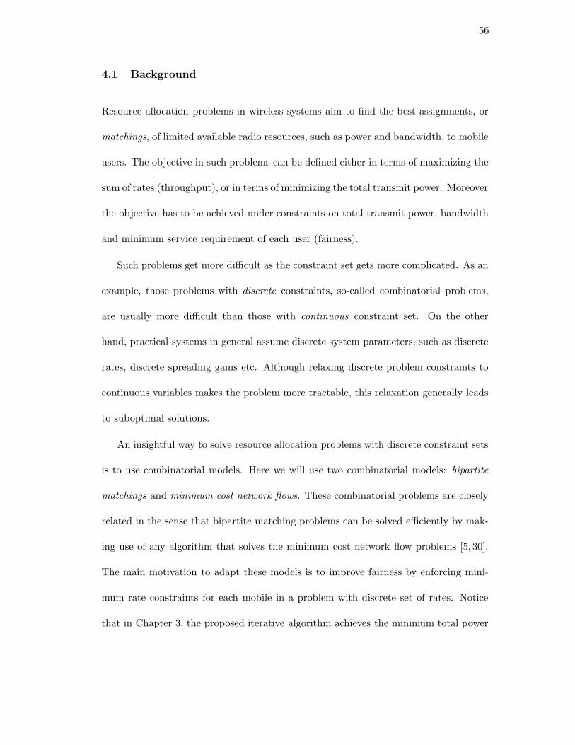
56

4.1 Background

Resource allocation problems in wireless systems aim to find the best assignments, or

matchings, of limited available radio resources, such as power and bandwidth, to mobile

users. The objective in such problems can be defined either in terms of maximizing the

sum of rates (throughput), or in terms of minimizing the total transmit power. Moreover

the objective has to be achieved under constraints on total transmit power, bandwidth

and minimum service requirement of each user (fairness).

Such problems get more difficult as the constraint set gets more complicated. As an

example, those problems with discrete constraints, so-called combinatorial problems,

are usually more difficult than those with continuous constraint set. On the other

hand, practical systems in general assume discrete system parameters, such as discrete

rates, discrete spreading gains etc. Although relaxing discrete problem constraints to

continuous variables makes the problem more tractable, this relaxation generally leads

to suboptimal solutions.

An insightful way to solve resource allocation problems with discrete constraint sets

is to use combinatorial models. Here we will use two combinatorial models: bipartite

matchings and minimum cost network flows. These combinatorial problems are closely

related in the sense that bipartite matching problems can be solved efficiently by mak-

ing use of any algorithm that solves the minimum cost network flow problems [5, 30].

The main motivation to adapt these models is to improve fairness by enforcing mini-

mum rate constraints for each mobile in a problem with discrete set of rates. Notice

that in Chapter 3, the proposed iterative algorithm achieves the minimum total power

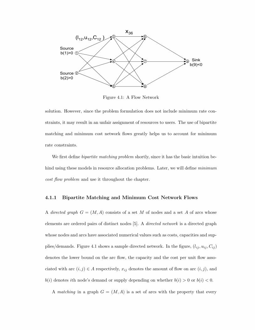
57

1

4

3

7

85

9

2

6(l12,u12,C12 )

x36

Source

b(1)>0

Sink

b(9)<0

Source

b(2)>0

Figure 4.1: A Flow Network

solution. However, since the problem formulation does not include minimum rate con-

straints, it may result in an unfair assignment of resources to users. The use of bipartite

matching and minimum cost network flows greatly helps us to account for minimum

rate constraints.

We first define bipartite matching problem shortly, since it has the basic intuition be-

hind using these models in resource allocation problems. Later, we will define minimum

cost flow problem and use it throughout the chapter.

4.1.1 Bipartite Matching and Minimum Cost Network Flows

A directed graph G = (M,A) consists of a set M of nodes and a set A of arcs whose

elements are ordered pairs of distinct nodes [5]. A directed network is a directed graph

whose nodes and arcs have associated numerical values such as costs, capacities and sup-

plies/demands. Figure 4.1 shows a sample directed network. In the figure, (lij , uij , Cij)

denotes the lower bound on the arc flow, the capacity and the cost per unit flow asso-

ciated with arc (i, j) ∈ A respectively, xij denotes the amount of flow on arc (i, j), and

b(i) denotes ith node’s demand or supply depending on whether b(i) > 0 or b(i) < 0.

A matching in a graph G = (M,A) is a set of arcs with the property that every

58

2

1

5

63

4

7

c14

c15c16

c37

c34

c27

c24

cij: arc cost

Figure 4.2: A Bipartite Network

node is incident to at most one arc in the set so that the matching results in a pairing

of the nodes in the graph using the arcs in A [5]. Matching problems on graphs with

two sets of nodes and with arcs that join only nodes between the two sets are called

bipartite matching problems. Figure 4.2 shows a sample bipartite graph and possible

matchings between the two sets of nodes connected by some arcs. Here we are interested

in weighted matching problems in which there is a weight associated with each arc, and

the objective is to minimize or maximize the total weight of the matching.

In our problem formulation, we will use the first set of nodes (or objects) on a

bipartite graph to represent network resources such as spreading codes, OFDM tones,

time slots etc., and the second set of nodes will represent the mobiles. Our target is to

find the matching between these two sets that has the minimum total weight (cost or

reward).

59

Although bipartite matching problems underlie the basic idea of resource allocation

problems, we will not go into further details of bipartite matchings in this chapter.

Instead, we will use the closely related minimum cost network flows formulation. There

are two reasons to use minimum cost flow model instead of bipartite matchings. First,

any bipartite matching problem can be expressed as a minimum cost network flow

problem; see [5, 30] for details. In other words, any algorithm that solves minimum

cost flow problems solves the bipartite matching problem as well. Second, as we will

show in the following sections that it is very easy to define minimum rate constraints

in a flow network by assigning lower bounds on the amount of flows on appropriate

arcs in the network. The inherent structure of bipartite matching does not have this

property, because any node in a set can at most be connected to a single node in the

other set. We refer to [5, 30] for further details on the relationship between these two

combinatorial models.

The definition of minimum cost flow problem is as follows [5, 30]. Let G = (M,A)

be a directed network with a cost Cij , capacity uij , a lowerbound on the arc flow lij

and flow xij associated with every arc (i, j) ∈ A. Associated with each node i ∈ M , a

number b(i) indicates ith node’s demand or supply depending on whether b(i) > 0 or

b(i) < 0. In this case the minimum cost flow problem is [5, 30]:

min∑

(i,j)∈A

Cijxij (4.1)

s.t.∑

{j:(i,j)∈A}

xij −∑

{j:(j,i)∈A}

xji = b(i) for all i ∈M

lij ≤ xij ≤ uij for all (i, j) ∈ A

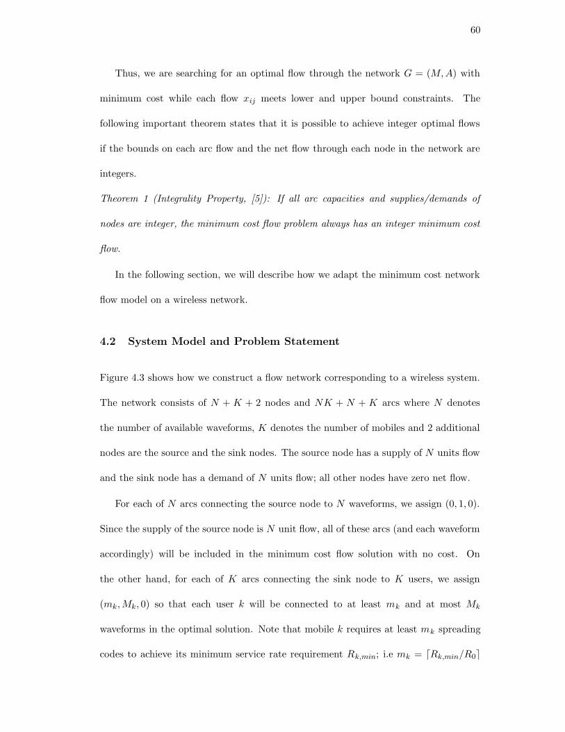
60

Thus, we are searching for an optimal flow through the network G = (M,A) with

minimum cost while each flow xij meets lower and upper bound constraints. The

following important theorem states that it is possible to achieve integer optimal flows

if the bounds on each arc flow and the net flow through each node in the network are

integers.

Theorem 1 (Integrality Property, [5]): If all arc capacities and supplies/demands of

nodes are integer, the minimum cost flow problem always has an integer minimum cost

flow.

In the following section, we will describe how we adapt the minimum cost network

flow model on a wireless network.


Figure 4.3 shows how we construct a flow network corresponding to a wireless system.

The network consists of N + K + 2 nodes and NK + N + K arcs where N denotes

the number of available waveforms, K denotes the number of mobiles and 2 additional

nodes are the source and the sink nodes. The source node has a supply of N units flow

and the sink node has a demand of N units flow; all other nodes have zero net flow.

For each of N arcs connecting the source node to N waveforms, we assign (0, 1, 0).

Since the supply of the source node is N unit flow, all of these arcs (and each waveform

accordingly) will be included in the minimum cost flow solution with no cost. On

the other hand, for each of K arcs connecting the sink node to K users, we assign

(mk,Mk, 0) so that each user k will be connected to at least mk and at most Mk

waveforms in the optimal solution. Note that mobile k requires at least mk spreading

codes to achieve its minimum service rate requirement Rk,min; i.e mk = dRk,min/R0e

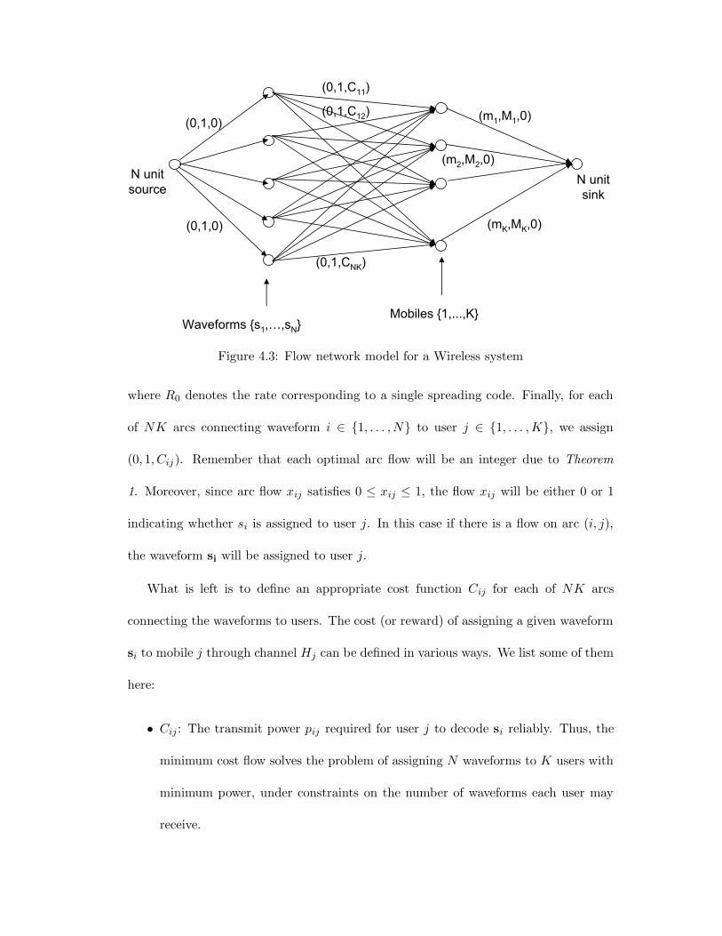
61

Waveforms {s1,…,sN}Mobiles {1,...,K}

(0,1,0)

(0,1,0)

(0,1,CNK)

(0,1,C11)

(0,1,C12) (m1,M1,0)

(mK,MK,0)

(m2,M2,0)N unit

sourceN unit

sink

Figure 4.3: Flow network model for a Wireless system

where R0 denotes the rate corresponding to a single spreading code. Finally, for each

of NK arcs connecting waveform i ∈ {1, . . . , N} to user j ∈ {1, . . . ,K}, we assign

(0, 1, Cij). Remember that each optimal arc flow will be an integer due to Theorem

1. Moreover, since arc flow xij satisfies 0 ≤ xij ≤ 1, the flow xij will be either 0 or 1

indicating whether si is assigned to user j. In this case if there is a flow on arc (i, j),

the waveform si will be assigned to user j.

What is left is to define an appropriate cost function Cij for each of NK arcs

connecting the waveforms to users. The cost (or reward) of assigning a given waveform

si to mobile j through channel Hj can be defined in various ways. We list some of them

here:

• Cij : The transmit power pij required for user j to decode si reliably. Thus, the

minimum cost flow solves the problem of assigning N waveforms to K users with

minimum power, under constraints on the number of waveforms each user may

receive.

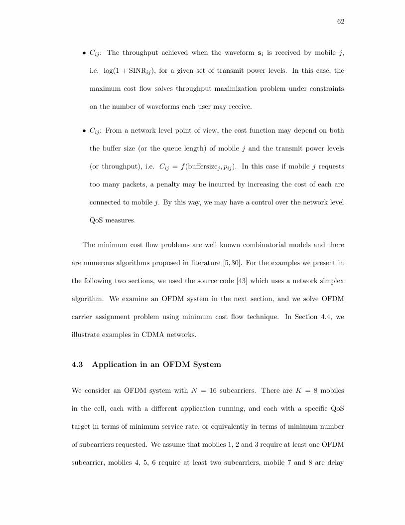
62

• Cij : The throughput achieved when the waveform si is received by mobile j,

i.e. log(1 + SINRij), for a given set of transmit power levels. In this case, the

maximum cost flow solves throughput maximization problem under constraints

on the number of waveforms each user may receive.

• Cij : From a network level point of view, the cost function may depend on both

the buffer size (or the queue length) of mobile j and the transmit power levels

(or throughput), i.e. Cij = f(buffersizej, pij). In this case if mobile j requests

too many packets, a penalty may be incurred by increasing the cost of each arc

connected to mobile j. By this way, we may have a control over the network level

QoS measures.

The minimum cost flow problems are well known combinatorial models and there

are numerous algorithms proposed in literature [5, 30]. For the examples we present in

the following two sections, we used the source code [43] which uses a network simplex

algorithm. We examine an OFDM system in the next section, and we solve OFDM

carrier assignment problem using minimum cost flow technique. In Section 4.4, we

illustrate examples in CDMA networks.

4.3 Application in an OFDM System

We consider an OFDM system with N = 16 subcarriers. There are K = 8 mobiles

in the cell, each with a different application running, and each with a specific QoS

target in terms of minimum service rate, or equivalently in terms of minimum number

of subcarriers requested. We assume that mobiles 1, 2 and 3 require at least one OFDM

subcarrier, mobiles 4, 5, 6 require at least two subcarriers, mobile 7 and 8 are delay

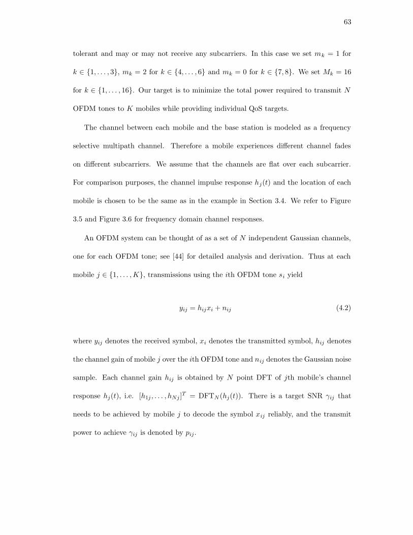
63

tolerant and may or may not receive any subcarriers. In this case we set mk = 1 for

k ∈ {1, . . . , 3}, mk = 2 for k ∈ {4, . . . , 6} and mk = 0 for k ∈ {7, 8}. We set Mk = 16

for k ∈ {1, . . . , 16}. Our target is to minimize the total power required to transmit N

OFDM tones to K mobiles while providing individual QoS targets.

The channel between each mobile and the base station is modeled as a frequency

selective multipath channel. Therefore a mobile experiences different channel fades

on different subcarriers. We assume that the channels are flat over each subcarrier.

For comparison purposes, the channel impulse response hj(t) and the location of each

mobile is chosen to be the same as in the example in Section 3.4. We refer to Figure

3.5 and Figure 3.6 for frequency domain channel responses.

An OFDM system can be thought of as a set of N independent Gaussian channels,

one for each OFDM tone; see [44] for detailed analysis and derivation. Thus at each

mobile j ∈ {1, . . . ,K}, transmissions using the ith OFDM tone si yield

yij = hijxi + nij (4.2)

where yij denotes the received symbol, xi denotes the transmitted symbol, hij denotes

the channel gain of mobile j over the ith OFDM tone and nij denotes the Gaussian noise

sample. Each channel gain hij is obtained by N point DFT of jth mobile’s channel

response hj(t), i.e. [h1j , . . . , hNj ]T = DFTN (hj(t)). There is a target SNR γij that

needs to be achieved by mobile j to decode the symbol xij reliably, and the transmit

power to achieve γij is denoted by pij.

64

We can express pij in terms of γij, σ2 and hij :

pij =γijσ

2

|hij |2(4.3)

In this case we choose the cost function to be Cij = pij. In the experiment, the

SNR target is 5 (7 dB) and σ2 = 10−13 W. The optimal solution is as follows. Mobile

1 receives one carrier corresponding to 1th OFDM tone, i.e. s1, mobile 2 receives one

carrier corresponding to 16th OFDM tone, mobile 3 receives one carrier corresponding

to 9th OFDM tone, mobile 4 receives two carriers corresponding to 8th and 10th OFDM

tones, mobile 5 receives two carriers corresponding to 7th and 13th OFDM tones, mobile

6 receives two carriers corresponding to 5th and 11th OFDM tones, mobile 7 does not

receive any OFDM tones, and mobile 8 receives seven subcarriers corresponding to

2nd, 3th, 4th, 6th, 12th, 14th and 15th OFDM tones. The total power required for the

optimal set of assignments is 4.44 Watts.

In case all mobiles are delay tolerant, i.e. mk = 0 for k = {1, . . . ,K}, mobile 4

receives one carrier corresponding to 9th OFDM tone, and mobile 8 receives the rest

of the OFDM tones. None of the other mobiles are served in this case. Observe in

Figure 3.5 and Figure 3.6 that each OFDM carrier is assigned to the mobile with the

largest gain over that subchannel in this case. The total power required for this set of

assignments is 0.45 Watts.

To compare the above numerical results with the CDMA example in Section 3.4,

notice that in case all mobiles are delay tolerant and minimum number of carrier require-

ments are all zero, a system using OFDM type multiaccess scheme requires more power

than a system using a CDMA type multiaccess scheme (≈ 0.45 Watts for OFDM and

65

≈ 0.03 Watts for CDMA). This result is counterintuitive since we might expect OFDM

type orthogonal transmission schemes to be more efficient than a CDMA scheme with

multiaccess interference in the context of power minimization. The reason for larger

transmit power in the case of an OFDM system is the requirement of the same SNR

on each subchannel. In this case, the transmitter allocates nonzero power even on sub-

channels with deep fades. In particular, this policy contradicts with the information

theoretic optimal water-filling policy where the channels with very deep fades are likely

to be allocated zero power [8].

4.4 Application in a CDMA System

Under a frequency selective multipath channel assumption, the problem of minimizing

total transmit power on the downlink of a multiaccess system with multirate services

has been studied in Chapter 3. In the case of a CDMA system, the proposed iterative

algorithm (3.11) converges to the optimal set of spreading code assignments (orthogonal

Walsh codes) to mobiles and to the set of optimal transmit power levels. On the other

hand, the problem definition in Chapter 3 does not include minimum QoS targets in

terms of number of spreading codes requested for each mobile. Thus, not all users

are guaranteed to be served, and the optimal algorithm (3.11) may result in an unfair

assignment of resources. In this section, we aim to allocate each user at least a number

of codes corresponding to its minimum QoS target while minimizing total transmit

power in a multipath channel on the downlink of a CDMA system.

We apply the same flow network model shown in Figure 4.3 for a CDMA system.

The cost Cij of an arc (i, j) connecting a spreading code si to a mobile j is defined

in terms of the transmit power pi required for mobile j to receive ith spreading code

66

with acceptable quality, i.e. achieving target SINR γ at the output of the receiver filter

fij (instead of using conventional notation cij for the receiver filter, we use fij for the

f ilter in order to avoid confusion with cost Cij). The SINR γij achieved at the output

of the receiver filter fij is

γij =pi(f

TijHjsi)

2

∑

v 6=i pv(fTijHjsv)2 + σ2(fT

ij fij)(4.4)

where Hj denotes the channel matrix of mobile j. In this case, the cost of an arc is

Cij = pi|γij=γ =γ(∑

v 6=i pv(fTijHjsv)

2 + σ2(fTij fij))

(fTijHjsi)2

(4.5)

Among all receiver filters, the MMSE filter minimizes (4.5) since it maximizes the

inverse of the cost function, i.e. SINR, see Section 3.3 for a similar analysis. Therefore

fij can be replaced by fMMSEij in (4.5). Notice that the cost structure (4.5) in a CDMA

system is fundamentally different than the cost structure (4.3) in an OFDM system.

While OFDM arc costs (4.3) are not dependent on each others, which is a result of

orthogonal transmission and reception, CDMA arc costs are dependent on each others

due to multiaccess interference. Notice that Cij (4.5) is a function of pv which is the

cost of another arc.

The following two sections present two approaches to resolve this issue.

4.4.1 CDMA Flow Network Model with Linear Receiver Processing

The fact that the flow network model applies well in case of an OFDM system inspires us

to orthogonalize CDMA channels in a way to get rid of mutual dependence of arc costs.

To this end, we combine the network flow approach with linear receiver processing in a

67

CDMA system.

For the sake of clarity, we revisit the transmitted signal vector x, and the received

signal vector rj by mobile j below. The definitions of each variable used in the expres-

sions are given in detail in Section 3.2.

x =

N∑

i=1

√pibisi (4.6)

rj =

N∑

i=1

√pibiHjsi + nj (4.7)

Linear receiver processing multiplies the received signal (4.7) by the inverse of the

channel matrix Hj. We assume that each mobile knows its own channel. The processed

received signal is denoted by rj

rj = H−1j rj = H−1

j (

N∑

i=1

√pibiHjsi + nj)

=

N∑

i=1

√pibisi + nj (4.8)

where nj = H−1j nj . By linear receiver processing, we orthogonalize received CDMA

waveforms at the expense of coloring the white receiver noise. This operation is reason-

able on the downlink of the system since all transmitted waveforms, both the desired

one and the interferer waveforms, get distorted by the same channel on the downlink.

Thus knowledge of mobile j’s channel Hj is good enough to restore the orthogonality of

the transmitted waveforms at mobile j’s receiver. Notice that this operation is similar

to zero forcing equalization in ISI channels.

The receiver filter fij, following receiver processing, matches to the spreading code

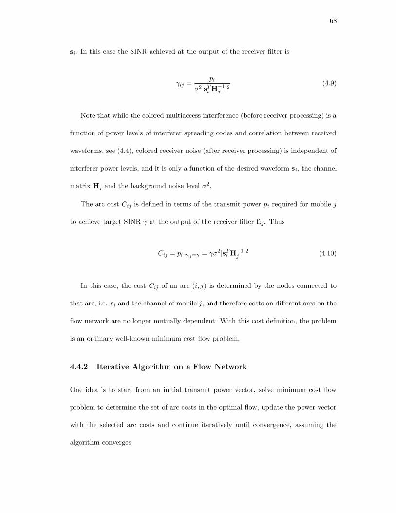
68

si. In this case the SINR achieved at the output of the receiver filter is

γij =pi

σ2|sTi H−1

j |2(4.9)

Note that while the colored multiaccess interference (before receiver processing) is a

function of power levels of interferer spreading codes and correlation between received

waveforms, see (4.4), colored receiver noise (after receiver processing) is independent of

interferer power levels, and it is only a function of the desired waveform si, the channel

matrix Hj and the background noise level σ2.

The arc cost Cij is defined in terms of the transmit power pi required for mobile j

to achieve target SINR γ at the output of the receiver filter fij. Thus

Cij = pi|γij=γ = γσ2|sTi H−1

j |2 (4.10)

In this case, the cost Cij of an arc (i, j) is determined by the nodes connected to

that arc, i.e. si and the channel of mobile j, and therefore costs on different arcs on the

flow network are no longer mutually dependent. With this cost definition, the problem

is an ordinary well-known minimum cost flow problem.

4.4.2 Iterative Algorithm on a Flow Network

One idea is to start from an initial transmit power vector, solve minimum cost flow

problem to determine the set of arc costs in the optimal flow, update the power vector

with the selected arc costs and continue iteratively until convergence, assuming the

algorithm converges.

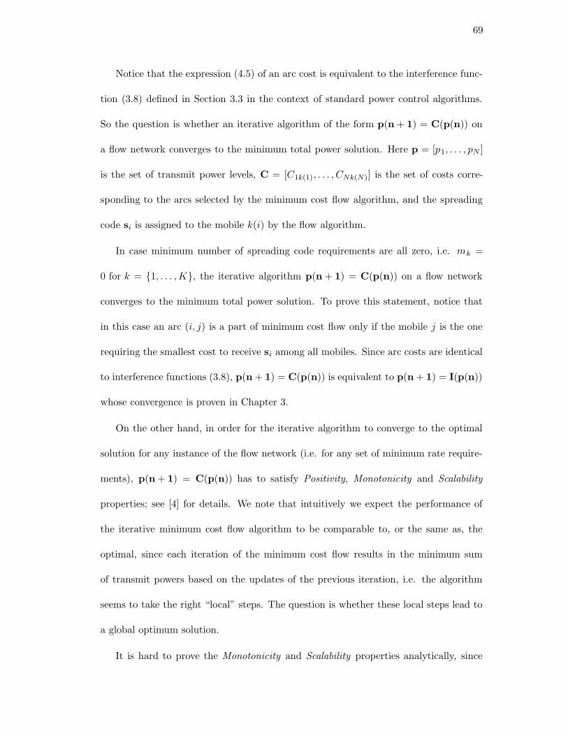
69

Notice that the expression (4.5) of an arc cost is equivalent to the interference func-

tion (3.8) defined in Section 3.3 in the context of standard power control algorithms.

So the question is whether an iterative algorithm of the form p(n + 1) = C(p(n)) on

a flow network converges to the minimum total power solution. Here p = [p1, . . . , pN ]

is the set of transmit power levels, C = [C1k(1), . . . , CNk(N)] is the set of costs corre-

sponding to the arcs selected by the minimum cost flow algorithm, and the spreading

code si is assigned to the mobile k(i) by the flow algorithm.

In case minimum number of spreading code requirements are all zero, i.e. mk =

0 for k = {1, . . . ,K}, the iterative algorithm p(n + 1) = C(p(n)) on a flow network

converges to the minimum total power solution. To prove this statement, notice that

in this case an arc (i, j) is a part of minimum cost flow only if the mobile j is the one

requiring the smallest cost to receive si among all mobiles. Since arc costs are identical

to interference functions (3.8), p(n + 1) = C(p(n)) is equivalent to p(n + 1) = I(p(n))

whose convergence is proven in Chapter 3.

On the other hand, in order for the iterative algorithm to converge to the optimal

solution for any instance of the flow network (i.e. for any set of minimum rate require-

ments), p(n + 1) = C(p(n)) has to satisfy Positivity, Monotonicity and Scalability

properties; see [4] for details. We note that intuitively we expect the performance of

the iterative minimum cost flow algorithm to be comparable to, or the same as, the

optimal, since each iteration of the minimum cost flow results in the minimum sum

of transmit powers based on the updates of the previous iteration, i.e. the algorithm

seems to take the right “local” steps. The question is whether these local steps lead to

a global optimum solution.

It is hard to prove the Monotonicity and Scalability properties analytically, since

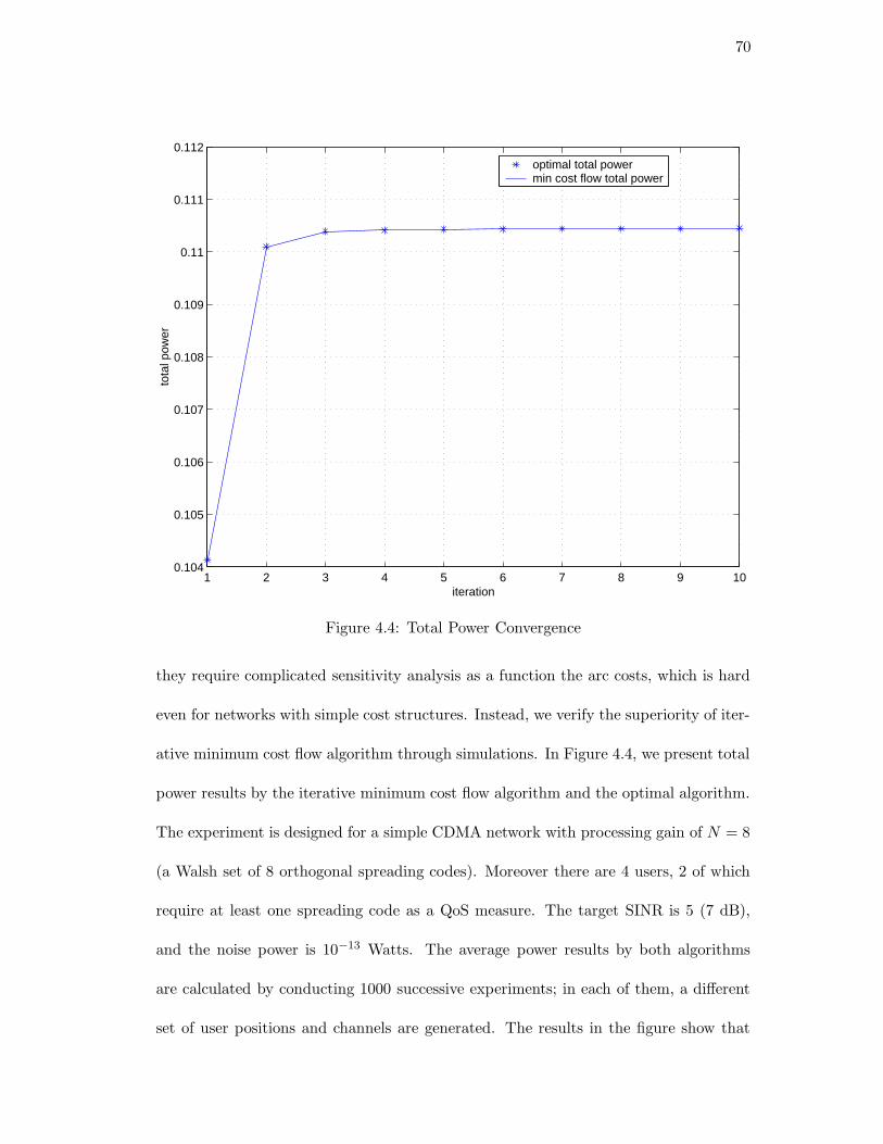
70

1 2 3 4 5 6 7 8 9 100.104

0.105

0.106

0.107

0.108

0.109

0.11

0.111

0.112

iteration

tota

l pow

eroptimal total powermin cost flow total power

Figure 4.4: Total Power Convergence

they require complicated sensitivity analysis as a function the arc costs, which is hard

even for networks with simple cost structures. Instead, we verify the superiority of iter-

ative minimum cost flow algorithm through simulations. In Figure 4.4, we present total

power results by the iterative minimum cost flow algorithm and the optimal algorithm.

The experiment is designed for a simple CDMA network with processing gain of N = 8

(a Walsh set of 8 orthogonal spreading codes). Moreover there are 4 users, 2 of which

require at least one spreading code as a QoS measure. The target SINR is 5 (7 dB),

and the noise power is 10−13 Watts. The average power results by both algorithms

are calculated by conducting 1000 successive experiments; in each of them, a different

set of user positions and channels are generated. The results in the figure show that

71

the iterative minimum cost flow algorithm achieves the minimum total power solution

under strict minimum rate constraints.


This chapter illustrates applications of combinatorial network flow models in wireless

resource management problems. The communication through a wireless network is

modeled as a network flow, and the target is to minimize the cost of information flow

through the network under constraints on demands (minimum rate) of mobiles and

supply (bandwidth) of the base station. We present examples in OFDM and CDMA

wireless networks to illustrate the use of the minimum cost flow model.

72

Chapter 5

Conclusion and Future Work

In this thesis, we investigate radio resource management for downlink wireless systems.

In the first part of the thesis, we examine how to maximize the network throughput on

the downlink of a multirate CDMA wireless network under constraints on total transmit

power and minimum QoS (rate) requirement of each user. The optimal algorithm is

determined as follows. First, users are ordered based on their transmit energy per bit

requirements to achieve the target received energy per bit to interference power spectral

density ratio at the receivers. Based on the initial ordering, we prove that for systems

employing multiple codes, the greedy rate scheduling is optimal, and therefore it yields

maximum network throughput. For systems employing OVSF codes, the greedy rate

scheduling is optimal if the minimum rate requirement of a user is larger than or equal

to the minimum rate requirement of any other user with a larger transmit energy

per bit requirement. Simulation results show that the greedy algorithm, even when

it is suboptimal, is a good heuristic yielding average throughput which is very close

to the optimal achievable throughput in OVSF-CDMA systems. The simplicity and

polynomial time complexity of the greedy algorithms seem to be very attractive from

an implementation point of view.

In the second part of the thesis, we investigate joint power control and orthogonal

code selection (rate control) in frequency selective multipath channels. We show that

73

the standard power control framework can be extended to include rate control as well.

Using this framework, we prove that a joint power and rate control algorithm converges

to optimum assignments of multiaccess resources (time slots for TDMA, spreading

codes for CDMA, subcarriers for OFDM etc.) to users, and to optimum transmit

power levels such that the total transmit power is minimized while each transmitted

bit can be decoded with sufficient SINR.

Finally, we show how to apply combinatorial network flow models in wireless re-

source management problems. We model the communication through a wireless network

as a network flow, and we minimize the cost of information flow through the network

under constraints on demands (minimum rate) of mobiles and supply (bandwidth) of

the base station. This model helps us to improve fairness by enforcing minimum rate

constraints on each mobile, and to deal with practical discrete system constraints. We

first apply minimum cost network flow idea in the case of an OFDM system where the

channel is flat on each subcarrier and frequency selective across the subcarriers. We

then combine the minimum cost network flow technique with linear receiver processing.

Finally, we propose an iterative minimum cost flow algorithm for CDMA systems.

74

References

[1] O. Awoniyi, N. Mehta, and L.J. Greenstein. Characterizing the OrthogonalityFactor in WCDMA Downlinks. IEEE Transactions on Wireless Communications.,2(4), July 2003.

[2] N.B. Mehta, L.J. Greenstein, III T.M Willis, and Z. Kostic. Analysis Results forthe Orthogonality Factor in WCDMA Downlinks. IEEE Transactions on WirelessCommunications, 2002. to be published.

[3] N.B. Mehta, L.J. Greenstein, III T.M Willis, and Z. Kostic. Analysis Results forthe Orthogonality Factor in WCDMA Downlinks. In Proc. of Veh. Technol. Conf.,pages 100–104, 2002.

[4] R. D. Yates. A Framework for Uplink Power Control in Cellular Radio Systems.IEEE Journal on Selected Areas in Communications, pages 1341–1347, September1995.

[5] R.K. Ahuja, T.L Magnanti, and J.B. Orlin. Network Flows. Prentice-Hall Inc.,1993.

[6] F. Adachi, M. Sawahashi, and H. Suda. Wideband DS-CDMA for Next-GenerationMobile Communication Systems. IEEE Communications Magazine, 36(9):56–69,September 1998.

[7] F. Adachi, M. Sawahashi, and K. Okawa. Tree-structured Generation of Orthogo-nal Spreading Codes with Different Lengths for Forward Link of DS-CDMA MobileRadio. IEEE Electronics Letters, 33(1):27–28, January 1997.

[8] T. Cover and J. Thomas. Elements of Information Theory. John Wiley Sons,1991.

[9] T. Minn and K.-Y Siu. Dynamic Assignment of Orthogonal Variable SpreadingFactor Codes in W-CDMA. IEEE J. Selected Areas Commun., 18(8):1429–1440,August 2000.

[10] A. Kam, T. Minn, and K.-Y Siu. Supporting Rate Guarantee and Fair Access forBursty Data Traffic in W-CDMA. IEEE J. Selected Areas Commun., 19(11):2121–2130, November 2001.

[11] Y-C. Tseng, C-M. Chao, and S-L Wu. Code Placement and Replacement Strategiesfor Wideband CDMA OVSF Code Tree Management. In Proc. of IEEE Globecom,volume 1, pages 562–566, 2001.

[12] M. Dell’Amico, M.L. Merani, and F. Maffioli. Efficient Algorithms for the As-signment of OVSF Codes in Wideband CDMA. In Proc. of ICC, volume 5, pages3055–3060, 2002.

75

[13] A. Sampath, P. S. Kumar, and J. M. Holtzman. Power control and resourcemanagement for a multimedia cdma wireless system. In Proc. of PIMRC, pages21–25, September 1995.

[14] S. Ramakrishna and J.M. Holtzman. A scheme for throughput maximization in adual-class cdma system. In Proc. of ICUPC, October 1997.

[15] S. Ulukus and L. J. Greenstein. Throughput maximization in cdma uplinks usingadaptive spreading and power control. In IEEE Symposium on Spread SpectrumTechniques and Applications, September 2000.

[16] S-J. Oh and K.M. Wasserman. Dynamic Spreading Gain Control in MultiserviceCDMA Networks. IEEE Journal on Selected Areas in Communications, 17(5),1999.

[17] S-J. Oh and K.M. Wasserman. Optimality of Greedy Power Control and VariableSpreading Gain in Multi-class CDMA Mobile Networks. In ACM/IEEE MobiCom,1999.

[18] J. B. Kim and M.L Honig. Resource Allocation for Multiple Classes of DS-CDMATraffic. IEEE Transactions on Vehicular Technology, 49:506–519, March 2000.

[19] F. Berggren and S.-L. Kim. Energy-Efficient Control of Rate and Power in DS-CDMA Systems. To appear in IEEE Transactions on Wireless Communications.

[20] A. Goldsmith S.A. Jafar. Adaptive Multirate CDMA for Uplink Throughput Max-imization. IEEE Transactions on Wireless Communications, 2(2):218–228, March2003.

[21] C. Saraydar, N. B. Mandayam, and D. J. Goodman. Efficient Power Control viaPricing in Wireless Data Networks. IEEE Trans. on Communications, 50(2):291–303, February 2002.

[22] C. Saraydar, N. B. Mandayam, and D. Goodman. Pricing and Power Control in aMulticell Wireless Data Network. IEEE JSAC, 19(10):1883–1892, October 2001.

[23] L. Song and N. Mandayam. Hierarchical SIR and Rate Control on the ForwardLink for CDMA Data Users under Delay and Error Constraints. IEEE JSAC,19(10):1871–1882, October 2001.

[24] F. Berggren, S.-L. Kim, R. Jntti, and J. Zander. Joint Power Control and Intra-cellScheduling of DS-CDMA Non-real Time Data. IEEE Journal on Selected Areasin Communications, 19(10):1860–1870, 2001.

[25] M. K. Karakayali, R. D. Yates, and L. Razumov. Joint Power and Rate Controlin Multiaccess Systems with Multirate Services. In CISS’03, The Johns HopkinsUniversity,MD, March 2003.

[26] C. Zhou, M.L Honig, S. Jordan, and R. Berry. Forward-link Resource Allocationfor a Two-cell Voice Network with Multiple Service Classes. volume 2, pages1060–1065, March 2003.

76

[27] L. Peijuan, M.L Honig, and S. Jordan. Forward-link CDMA Resource AllocationBased on Pricing. volume 3, pages 1410–1414, September 2000.

[28] J. W. Lee, R. Mazumdar, and N. B. Shroff. Joint Power and Data Rate Allocationfor the Downlink in Multi-class CDMA Wireless Networks. In The Fortieth AnnualAllerton Conference on Communication, Control, and Computing, Monticello, IL,October 2002.

[29] J. W. Lee, R. Mazumdar, and N. B. Shroff. Downlink Power Allocation for Multi-class CDMA Wireless Networks. In IEEE INFOCOM’02, New York, NY, June2002.

[30] C.H. Papadimitriou and K. Steiglitz. Combinatorial Optimization: Algorithms andComplexity. Dover Publications, 1998.

[31] Janne Laakso, Riku Jntti, and Mika Rinne Oscar Salonaho. Radio Resource Knap-sack Packing for WCDMA Air Interface. In Proc. of PIMRC, volume 1, 1998.

[32] S. Martello and P. Toth. Knapsack Problems. J. Wiley and Sons, 1990.

[33] V. Erceg, L.J. Greenstein, S.Y. Tjandra, S.R. Parkoff, A. Gupta, B. Kulic, A.A.Julius, and R. Bianchi. An Empirically Based Path Loss Model for Wireless Chan-nels in Suburban Environments. IEEE JSAC, 17(7), July 1999.

[34] S.V. Hanly and D. Tse. Power Control and Capacity of Spread-Spectrum WirelessNetworks. Automatica, pages 1987–2012, December 1999.

[35] S.-L. Kim, Z. Rosberg, and J. Zander. Combined Power Control and TransmissionRate Selection in Cellular Networks. In Proc. of VTC Fall, pages 1653–1657, 1999.

[36] B. Hashem and E. Sousa. A combined power/rate control scheme for data trans-mission over a ds/cdma system. In Proc. of IEEE VTC, May 1998.

[37] S. Kim and Y.H. Lee. Combined Rate and Power Adaptation in DS/CDMA Com-munications over Nakagami Fading Channels. IEEE Transactions on Communi-cations, 48, January 2000.

[38] S. Ulukus and R.D. Yates. Adaptive Power Control and MMSE Interference Sup-pression. Baltzer/ACM Wireless Networks, pages 4(6):489–496, 1998.

[39] Sergio Verdu. Multiuser Detection. Cambridge University Press, 1998.

[40] http://grouper.ieee.org/groups/802/16/tg1/phy/contrib/. Recommendation onchannel propagation model for local multipoint distribution service. 16th report.

[41] http://grouper.ieee.org/groups/802/16/tg1/phy/contrib/. Multipath measure-ments and modelling for fixed broadband wireless systems in a residential envi-ronment. 1th report.

[42] Arib swg2, specifications of air-interface for 3g mobile system. December 1998.volume 3.

[43] http://www.zib.de/Optimization/Software/Mcf.

77

[44] J. Beek, O. Edfors, M. Sandell, S. K. Wilson, and P.O. Borjesson. On channelestimation in ofdm systems. In Proc. of VTC, September 1995.

Documents

RESOURCE MANAGEMENT FOR DOWNLINK WIRELESS SYSTEMS