Embed Size (px)
Citation preview
Resonant Excitons in Strontium Titanate
Name: Tan Chian Wen Melvin
Matriculation Number: A0111064Y
Supervisor:
Assistant Professor Andrivo Rusydi
National University of Singapore
A thesis submitted to the Faculty of Science
as a partial fulfilment of the Bachelors of
Science (Hons.) in Physics
2017

Acknowledgements
I would like to express my greatest gratitude to Professor Andrivo
Rusydi for his patience and guidance throughout the project. I would
also like to thank Dr Pranjal for his help and answering my queries. Last
but not least, I would like to thank my family and friends who have
encouraged and supported me through the project.

1
Contents Abstract ......................................................................................................................................................... 2
Chapter 1: Introduction ................................................................................................................................ 3
1.1 Electromagnetic waves ....................................................................................................................... 3
1.2 Fresnel equations ................................................................................................................................ 6
1.3 Dielectric polarization ......................................................................................................................... 7
1.4 Permittivity.......................................................................................................................................... 8
1.5 Kramers-Kronig relations .................................................................................................................. 10
1.6 Excitons ............................................................................................................................................. 11
1.7 Spectroscopic ellipsometry ............................................................................................................... 13
1.8 Strontium Titanate ............................................................................................................................ 15
Chapter 2: Data Analysis Methodology ...................................................................................................... 16
2.1 Experiment background .................................................................................................................... 16
2.2 Experimental determination of the complex dielectric function ..................................................... 17
2.3 Curve Fitting of the complex dielectric function peaks .................................................................... 18
2.4 The curve fitting procedure .............................................................................................................. 20
2.5 Kramers-Kronig transformations of the curves of best fit ................................................................ 27
Chapter 3: Results and Discussion .............................................................................................................. 29
3.1 The curve fitting results .................................................................................................................... 29
3.2 The Kramers-Kronig transformation results ..................................................................................... 36
Chapter 4: Conclusion & Future Work ........................................................................................................ 42
4.1 Conclusion ......................................................................................................................................... 42
4.2 Future work ....................................................................................................................................... 43
References .................................................................................................................................................. 44
2
Abstract
Optical transitions play a role in the formation of excitons in Stontium Titanate (STO). It is
known that the interband transitions between the valence band of STO to the conduction band of
STO is the contributor of the Wannier excitons that are found in STO when a STO sample is
irradiated with light. Resonant excitons in STO on the other hand, are the result of optical
transitions between higher energy states. By curve fitting of the resonant excitonic peaks of the
imaginary part of the temperature difference data of the complex dielectric function of STO
obtained through spectroscopic ellipsometry and subsequently inputting the curve of best fit into
the a Kramers-Kronig transformation, we obtain the corresponding “curve of best fit” for the real
part of the temperature difference data of the complex dielectric function of STO. By comparing
this result to the experimental data points of the real part of the temperature difference data of the
complex dielectric function of STO, we deduce if the majority of the optical transitions between
these higher energy states responsible for the resonant exciton are interband transitions. In
addition, we also determine the sample quality of STO used in terms of the presence of
impurities and defects via the curve fitting procedure.
3
Chapter 1: Introduction
In this section, the background of spectroscopic ellipsometry, electromagnetic waves, behaviour
of electromagnetic waves as they transit from one medium to another and of dielectrics in the
presence of an applied external electric field is discussed. In addition, we discuss the various
exciton types and a brief description of STO.
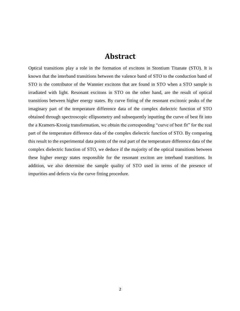
1.1 Electromagnetic waves
Electromagnetic waves travel at a constant speed, the speed of light in a vacuum or air medium.
They arise from two oscillating electric and magnetic fields that oscillate about one another and
are lying in planes perpendicular to each other. The wave propagation in three dimensional space
for the oscillating electric field vector component and oscillating magnetic field vector
component can be described by the following relations (1.1.1) and (1.1.2) respectively.
Here, is the amplitude of the electric field oscillation, is the amplitude of the magnetic
field oscillation, is the angular frequency, is the wave vector and is the phase angle. The
picture below illustrates the propagation of an electromagnetic wave.
Fig 1.1.1: An electromagnetic wave propagating in three dimensional space [1]
4
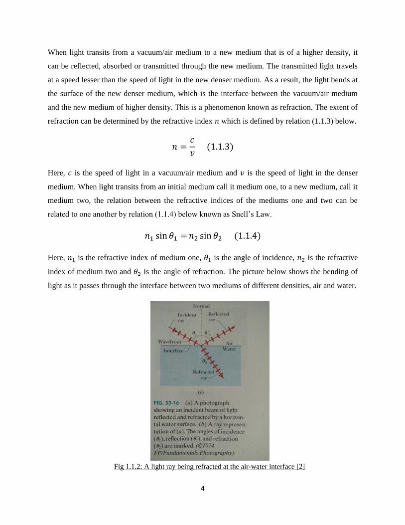
When light transits from a vacuum/air medium to a new medium that is of a higher density, it
can be reflected, absorbed or transmitted through the new medium. The transmitted light travels
at a speed lesser than the speed of light in the new denser medium. As a result, the light bends at
the surface of the new denser medium, which is the interface between the vacuum/air medium
and the new medium of higher density. This is a phenomenon known as refraction. The extent of
refraction can be determined by the refractive index which is defined by relation (1.1.3) below.
Here, is the speed of light in a vacuum/air medium and is the speed of light in the denser
medium. When light transits from an initial medium call it medium one, to a new medium, call it
medium two, the relation between the refractive indices of the mediums one and two can be
related to one another by relation (1.1.4) below known as Snell’s Law.
Here, is the refractive index of medium one, is the angle of incidence, is the refractive
index of medium two and is the angle of refraction. The picture below shows the bending of
light as it passes through the interface between two mediums of different densities, air and water.
Fig 1.1.2: A light ray being refracted at the air-water interface [2]
5
When the refraction of light is accompanied by the attenuation of light as light passes through the
optical medium, the refractive index is no longer a real value but a complex value.
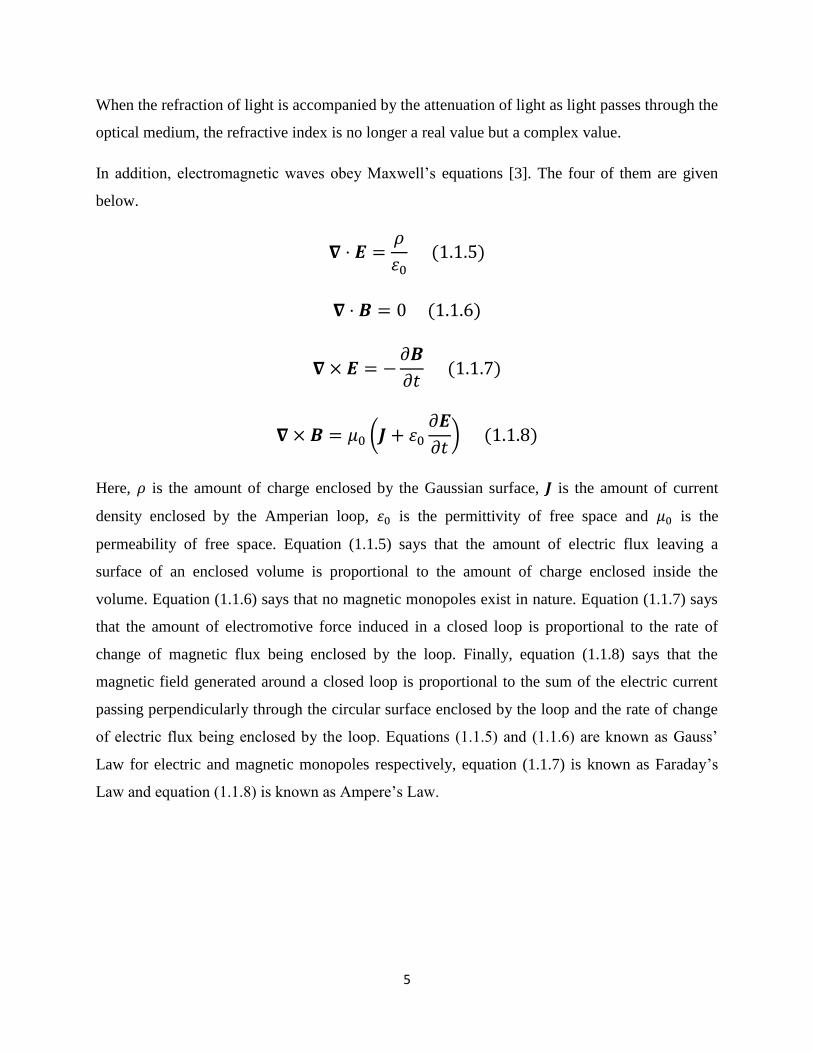
In addition, electromagnetic waves obey Maxwell’s equations [3]. The four of them are given
below.
Here, is the amount of charge enclosed by the Gaussian surface, is the amount of current
density enclosed by the Amperian loop, is the permittivity of free space and is the
permeability of free space. Equation (1.1.5) says that the amount of electric flux leaving a
surface of an enclosed volume is proportional to the amount of charge enclosed inside the
volume. Equation (1.1.6) says that no magnetic monopoles exist in nature. Equation (1.1.7) says
that the amount of electromotive force induced in a closed loop is proportional to the rate of
change of magnetic flux being enclosed by the loop. Finally, equation (1.1.8) says that the
magnetic field generated around a closed loop is proportional to the sum of the electric current
passing perpendicularly through the circular surface enclosed by the loop and the rate of change
of electric flux being enclosed by the loop. Equations (1.1.5) and (1.1.6) are known as Gauss’
Law for electric and magnetic monopoles respectively, equation (1.1.7) is known as Faraday’s
Law and equation (1.1.8) is known as Ampere’s Law.
6
1.2 Fresnel equations
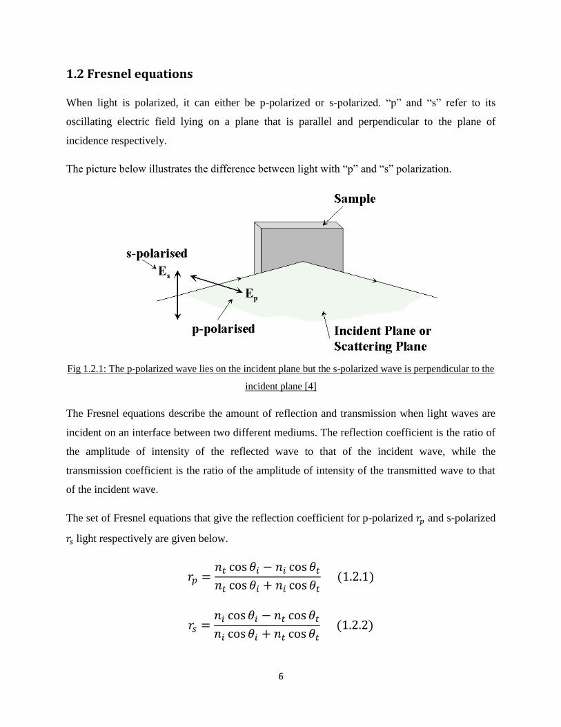
When light is polarized, it can either be p-polarized or s-polarized. “p” and “s” refer to its
oscillating electric field lying on a plane that is parallel and perpendicular to the plane of
incidence respectively.
The picture below illustrates the difference between light with “p” and “s” polarization.
Fig 1.2.1: The p-polarized wave lies on the incident plane but the s-polarized wave is perpendicular to the
incident plane [4]
The Fresnel equations describe the amount of reflection and transmission when light waves are
incident on an interface between two different mediums. The reflection coefficient is the ratio of
the amplitude of intensity of the reflected wave to that of the incident wave, while the
transmission coefficient is the ratio of the amplitude of intensity of the transmitted wave to that
of the incident wave.
The set of Fresnel equations that give the reflection coefficient for p-polarized and s-polarized
light respectively are given below.
7
The set of Fresnel equations that give the transmission coefficient for p-polarized and s-
polarized light respectively are given below.
Here, is the angle of incidence, is the angle of transmission, is the refractive index of the
medium the incident ray passes through and is the refractive index of the medium the
transmission ray passes through.
The Fresnel equations also apply to mediums with complex refractive indices.
1.3 Dielectric polarization
A dielectric material is in general a material where all charges are not free to move around the
material like in conductors, but are tightly attached to their respective atoms or molecules.
However, they are given some extent to move about within their respective atoms or molecules.
When an external electric field is applied on a dielectric material, the positively charged nucleus
and the negatively charged electron cloud within each atom or molecule experience an electric
force in opposite directions causing them to move apart from each other in opposite directions.
They move apart from each other until equilibrium is reached when the mutual forces of
attraction holding them together are balanced by the forces of repulsion they experience as a
result of the applied external electric field. This results in a slight shift of the positive charges in
one direction and the negative charges in the opposite direction. Every atom or molecule
possesses a small dipole moment as a result, which points in the opposite direction of the applied
external electric field. The dielectric as a whole will have a net dipole moment pointing in the
opposite direction of the applied external electric field contributed from the sum of all the small
dipole moments of individual constituent atoms or molecules. This phenomenon is known as
dielectric polarization. The extent of polarization is typically measured by the number of dipole
moments per unit volume and is a vector quantity denoted by .
8
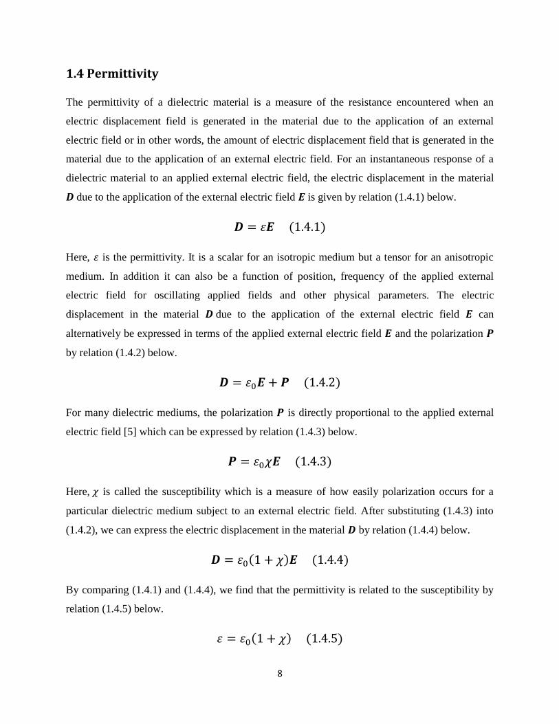
1.4 Permittivity
The permittivity of a dielectric material is a measure of the resistance encountered when an
electric displacement field is generated in the material due to the application of an external
electric field or in other words, the amount of electric displacement field that is generated in the
material due to the application of an external electric field. For an instantaneous response of a
dielectric material to an applied external electric field, the electric displacement in the material
due to the application of the external electric field is given by relation (1.4.1) below.
Here, is the permittivity. It is a scalar for an isotropic medium but a tensor for an anisotropic
medium. In addition it can also be a function of position, frequency of the applied external
electric field for oscillating applied fields and other physical parameters. The electric
displacement in the material due to the application of the external electric field can
alternatively be expressed in terms of the applied external electric field and the polarization
by relation (1.4.2) below.
For many dielectric mediums, the polarization is directly proportional to the applied external
electric field [5] which can be expressed by relation (1.4.3) below.
Here, is called the susceptibility which is a measure of how easily polarization occurs for a
particular dielectric medium subject to an external electric field. After substituting (1.4.3) into
(1.4.2), we can express the electric displacement in the material by relation (1.4.4) below.
By comparing (1.4.1) and (1.4.4), we find that the permittivity is related to the susceptibility by
relation (1.4.5) below.
9
Physically, this means that when a particular dielectric medium polarizes more easily, the lesser
the resistance encountered when an electric displacement field is generated in the material due to
the application of an external electric field.
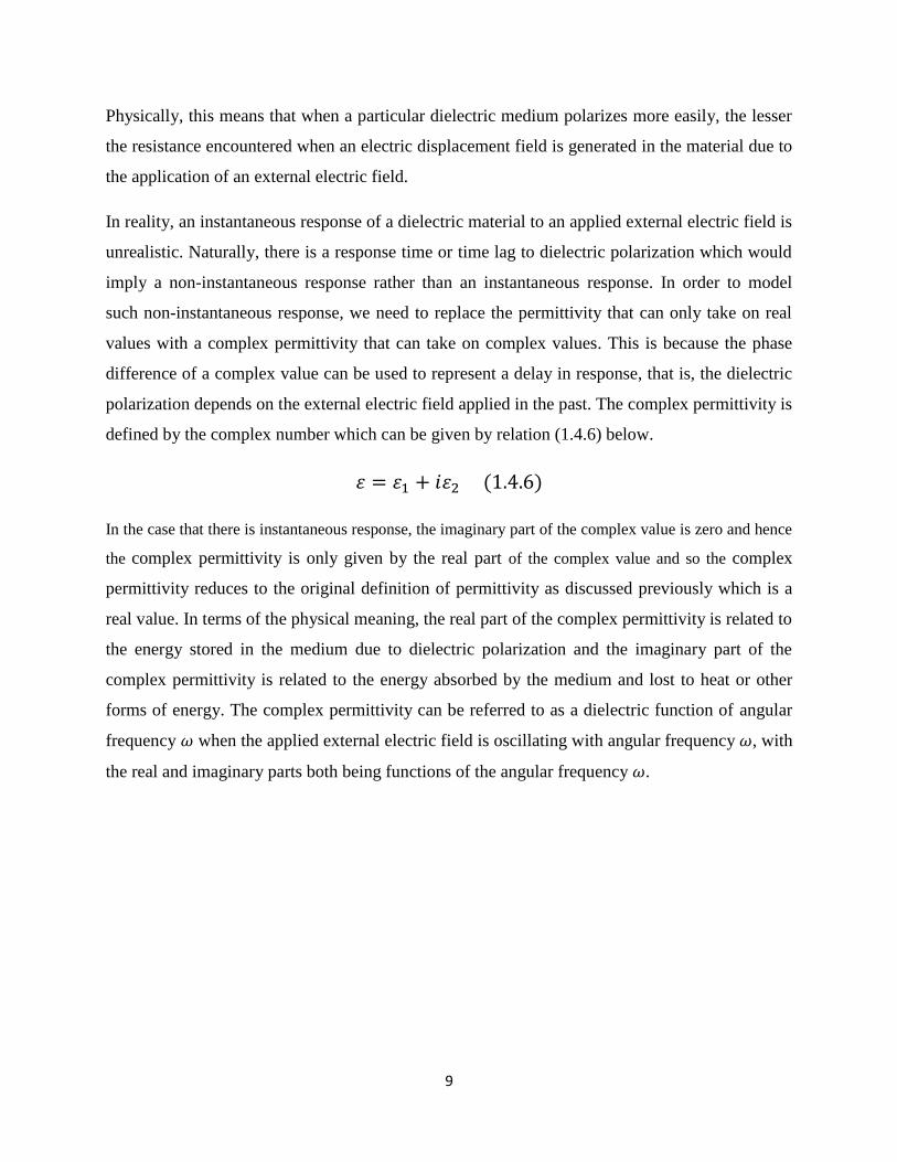
In reality, an instantaneous response of a dielectric material to an applied external electric field is
unrealistic. Naturally, there is a response time or time lag to dielectric polarization which would
imply a non-instantaneous response rather than an instantaneous response. In order to model
such non-instantaneous response, we need to replace the permittivity that can only take on real
values with a complex permittivity that can take on complex values. This is because the phase
difference of a complex value can be used to represent a delay in response, that is, the dielectric
polarization depends on the external electric field applied in the past. The complex permittivity is
defined by the complex number which can be given by relation (1.4.6) below.
In the case that there is instantaneous response, the imaginary part of the complex value is zero and hence
the complex permittivity is only given by the real part of the complex value and so the complex
permittivity reduces to the original definition of permittivity as discussed previously which is a
real value. In terms of the physical meaning, the real part of the complex permittivity is related to
the energy stored in the medium due to dielectric polarization and the imaginary part of the
complex permittivity is related to the energy absorbed by the medium and lost to heat or other
forms of energy. The complex permittivity can be referred to as a dielectric function of angular
frequency when the applied external electric field is oscillating with angular frequency , with
the real and imaginary parts both being functions of the angular frequency .
10
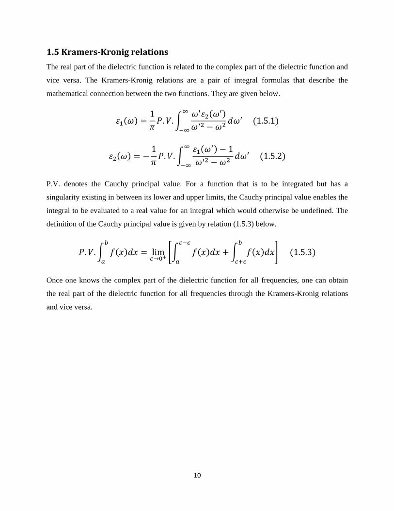
1.5 Kramers-Kronig relations
The real part of the dielectric function is related to the complex part of the dielectric function and
vice versa. The Kramers-Kronig relations are a pair of integral formulas that describe the
mathematical connection between the two functions. They are given below.
P.V. denotes the Cauchy principal value. For a function that is to be integrated but has a
singularity existing in between its lower and upper limits, the Cauchy principal value enables the
integral to be evaluated to a real value for an integral which would otherwise be undefined. The
definition of the Cauchy principal value is given by relation (1.5.3) below.
Once one knows the complex part of the dielectric function for all frequencies, one can obtain
the real part of the dielectric function for all frequencies through the Kramers-Kronig relations
and vice versa.
11
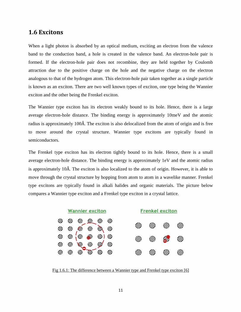
1.6 Excitons
When a light photon is absorbed by an optical medium, exciting an electron from the valence
band to the conduction band, a hole is created in the valence band. An electron-hole pair is
formed. If the electron-hole pair does not recombine, they are held together by Coulomb
attraction due to the positive charge on the hole and the negative charge on the electron
analogous to that of the hydrogen atom. This electron-hole pair taken together as a single particle
is known as an exciton. There are two well known types of exciton, one type being the Wannier
exciton and the other being the Frenkel exciton.
The Wannier type exciton has its electron weakly bound to its hole. Hence, there is a large
average electron-hole distance. The binding energy is approximately 10meV and the atomic
radius is approximately 100 . The exciton is also delocalized from the atom of origin and is free
to move around the crystal structure. Wannier type excitons are typically found in
semiconductors.
The Frenkel type exciton has its electron tightly bound to its hole. Hence, there is a small
average electron-hole distance. The binding energy is approximately 1eV and the atomic radius
is approximately 10 . The exciton is also localized to the atom of origin. However, it is able to
move through the crystal structure by hopping from atom to atom in a wavelike manner. Frenkel
type excitons are typically found in alkali halides and organic materials. The picture below
compares a Wannier type exciton and a Frenkel type exciton in a crystal lattice.
Fig 1.6.1: The difference between a Wannier type and Frenkel type exciton [6]
12
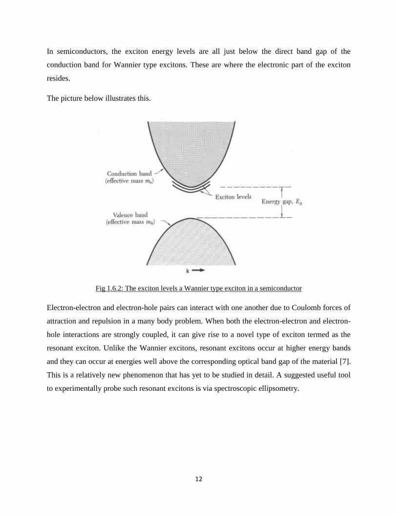
In semiconductors, the exciton energy levels are all just below the direct band gap of the
conduction band for Wannier type excitons. These are where the electronic part of the exciton
resides.
The picture below illustrates this.
Fig 1.6.2: The exciton levels a Wannier type exciton in a semiconductor
Electron-electron and electron-hole pairs can interact with one another due to Coulomb forces of
attraction and repulsion in a many body problem. When both the electron-electron and electron-
hole interactions are strongly coupled, it can give rise to a novel type of exciton termed as the
resonant exciton. Unlike the Wannier excitons, resonant excitons occur at higher energy bands
and they can occur at energies well above the corresponding optical band gap of the material [7].
This is a relatively new phenomenon that has yet to be studied in detail. A suggested useful tool
to experimentally probe such resonant excitons is via spectroscopic ellipsometry.
13
1.7 Spectroscopic ellipsometry
Spectroscopic ellipsometry is an experimental technique that studies the change in polarized light
upon the reflection and transmission of light in an optical medium. The measured optical
properties of the medium are the amplitude ratio and the phase difference between the p-
polarized and s-polarized light waves. Spectroscopic ellipsometry is typically carried out in the
infrared-visible to ultraviolet region. Spectroscopic ellipsometry measures the spectra
across a continuous range of incident photon energies . Here, is the Planck’s constant and
is the frequency of the incident photon. Subsequently, an optical model that assumes the medium
has a perfectly flat surface and infinite thickness is employed to obtain the pseudo dielectric
function (PDF) directly from the spectra. If the medium is isotropic and atomically
flat, then the PDF approaches the true dielectric function . Spectroscopic ellipsometry plays
an important role in the study of excitonic effects as it is able to probe neutral excitations that
give rise to electron-hole pairs and excitons.
The complex reflectance ratio is defined by relation (1.7.1) below.
When light reflection is measured in spectroscopic ellipsometry, the amplitude ratio and the
phase difference between the p-polarized and s-polarized light waves are related to the
complex reflectance ratio by relation (1.7.2) below.
Here, is the amplitude ratio between the reflected p-polarized and s-polarized light waves and
is the phase difference between the reflected p-polarized and s-polarized light waves.
The PDF can be obtained by relation (1.7.3) below.
14
Here, is the angle of incidence of the light beam which is pre-determined in the spectroscopic
ellipsometry experiment and is the complex reflectance ratio which can be found directly
using (1.7.2) with values obtained from the spectra which is measured during the
spectroscopic ellipsometry experiment. Assuming the medium used in the spectroscopic
ellipsometry experiment to be isotropic and atomically flat, the true dielectric function can be
considered to be equivalent to the PDF and can hence be given by (1.7.3).
General restrictions that have to be imposed on the optical medium being used for spectroscopic
ellipsometry are that the surface roughness of the sample is small and the measurements have to
be conducted at an oblique incidence. The rational for the former being that the light scattered by
a rough surface reduces the reflected light intensity severely, rendering the polarization state
difficult to measure. The rationale for the latter being that at normal incidence, p-polarized and s-
polarized waves cannot be distinguished making measurements of the polarization state
impossible [8].
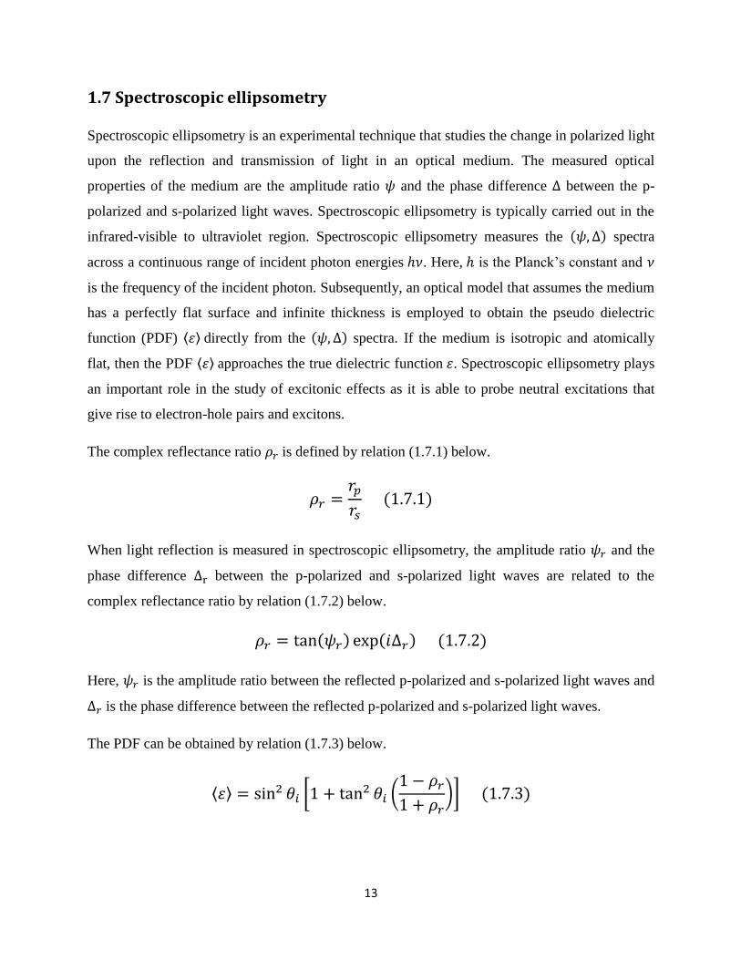
The picture below shows how spectroscopic ellipsometry works.
Fig 1.7.1: Spectroscopic ellipsometry on a sample
A beam of light is incident on the medium at a fixed angle of incidence . The medium has an
intrinsic refractive index which affects the amplitude ratio and extinction coefficient
which affects the phase difference . The reflected light is measured by a detector which records
the spectra across a continuous range of incident photon energies.
15
1.8 Strontium Titanate
Strontium titanate (STO) is a perovskite-type titanate. A perovskite is a material that has the
same crystal structure as calcium titanate. A perovskite has a general chemical formula ABX3
where A and B represent cations of different sizes and X is an anion.
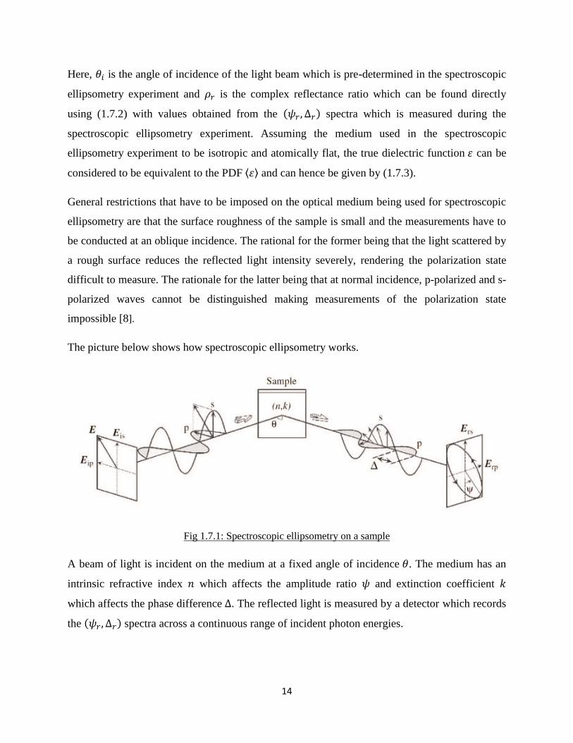
The crystal structure of STO is shown in the picture below.
Fig 1.8.1: The crystal structure of STO or a perovskite in general [9]
The Wannier exciton in STO has its electronic part well localized on the Ti atom, while the hole
is localized on the neighbouring O atom [10]. STO has a band gap of 3.2eV separating the
valence and conduction band at zero Kelvin [11]. The six fold coordination of Ti ions by
surrounding O ions result in a crystal field splitting of the degenerate Ti-3d states at 2.4eV into
two states Ti-3d t2g and Ti-3d eg. Speaking in terms of bands, the valence band of STO which is
the band with highest occupied molecular orbitals is the mainly the O-2s and O-2p states of
oxygen and the conduction band which is the band with lowest unoccupied molecular orbitals is
mainly the titanium empty Ti-3d states of titanium.
There are all together three excitonic peaks for STO named Ex1, Ex2 and Ex3. The Ex1 peak at
3.75eV at 4.2K is identified as a Wannier excitonic peak while the Ex2 and Ex3 peaks at 4.67eV
and 6.11eV respectively at 4.2K are identified as resonant excitonic peaks [12].

16
Chapter 2: Data Analysis Methodology
In this section, we will discuss a brief overview of the spectroscopic ellipsometry procedure used
to generate the data that is being collected for the data analysis. We will then discuss the curve
fitting procedure with the aid of Mathematica for the temperature difference of the imaginary
component of the complex dielectric function of STO. This will be followed by a discussion on
the application of the Kramers-Kronig relations on the curve fitted function of the temperature
difference of the imaginary component of the complex dielectric function to obtain the graph of
the temperature difference of the real component of the complex dielectric function of STO with
the aid of Mathematica. Last but not least, the graph of the temperature difference of the real
component of the complex dielectric function generated from the above procedure is compared
to the experimental data of the temperature difference of the real component of the complex
dielectric function of STO for analysis.
2.1 Experiment background
STO (100) samples from Crystec are being used for the spectroscopic ellipsometry
measurements. They are all of size 10mm by 10mm by 0.5mm and single side polished with rms
roughness less than 5 . Spectroscopic ellipsometry is carried out with a commercial rotating
analyser ellipsometer from J.A. Woollam Inc which covers a photon energy range from 0.6eV to
6.5eV in steps of 0.02eV. The lowest temperature that the STO samples are at is 4.2K and the
highest temperature that the STO samples are at is 350K. The low temperature measurements are
carried out in an open cycle cryostat with base pressures within the regime of Torr, created
by a mixture of liquid helium and liquid nitrogen. The angle of incidence for all measurements
made by the cryostat is fixed at 70 .
17
2.2 Experimental determination of the complex dielectric function
The STO samples are measured in air. Hence, the optical model employed is an air-sample
interface. The optical model also assumes a sample of infinite thickness. This assumption is valid
as the depth of the STO sample is much greater than the light beam penetration depth which does
not exceed 1 m. In addition, the optical model assumes an atomically flat surface which is valid
because all the STO samples have rms roughness less than 5 . Hence, the PDF which is
experimentally obtained directly from the spectroscopic ellipsometry measurements can be
considered to be the true complex dielectric function of STO.
18
2.3 Curve Fitting of the complex dielectric function peaks
The analysis of the peak data points obtained from spectroscopic ellipsometry requires
knowledge of the dielectric function pertaining to the sample. However, we do not know the
dielectric functions pertaining to the sample. We attempt to curve fit the peaks with bell-shaped
distributions, namely the Gaussian, Lorentz and Voigt profile.
We curve fit the imaginary component of the complex dielectric function as it is the imaginary
component that is dependent on the energy absorption of the material, which is in turn linked to
the material’s behavior in terms of photon absorption in order to form the exciton.
The Gaussian profile is a Gaussian distribution defined by relation (2.3.1) below.
Here, are parameters that describe the height of the peak, the position and the
standard deviation of the bell-shaped curve of the Gaussian distribution respectively. Note that
that the standard deviation is related to the half-width at half-maximum of the bell-shaped curve
of the Gaussian distribution.
The Lorentz profile is a Cauchy distribution defined by relation (2.3.2) below.
Here, are parameters that describe the height of the peak, the position and the scale
parameter determining the half-width at half-maximum of the bell-shaped curve of the Cauchy
distribution respectively. It is worth to mention that the Lorentz profile looks like a Gaussian
profile with a bell-shape but with lighter tails, that is, tails that go down less rapidly.
The Voigt profile is a profile that is obtained from the convolution of the Gaussian profile and
the Lorentz profile. The Voigt profile is defined by relation (2.3.3) which follows where the
asterisk is the notation for a convolution operation.
19
For the convenience of computation, the Voigt profile is often approximated by the pseudo-Voigt
profile which is much easier to work with [13]. The pseudo-Voigt profile is given by the linear
combination of or a weighted sum of the Gaussian and Lorentz profiles. The pseudo-Voigt
profile is defined by relation (2.3.4) below.
Here, and are the weights attached to the Gaussian profile and the Lorentz profile
respectively and they must both sum to unity and hence, is a value that must be bounded below
by zero and bounded above by one. In addition, the parameters in the pseudo-Voigt
profile must be same for both the Gaussian profile and the Lorentz profile involved.
20
2.4 The curve fitting procedure
The experimental data of the temperature difference of the imaginary component and real
component of the complex dielectric function of STO is obtained from the Singapore
Synchrotron Light Source (SSLS). The temperature difference of the imaginary component of
the complex dielectric function is defined by relation (2.4.1) that follows.
Here, takes the value 1 for the real component and the value 2 for the imaginary component.
is the temperature the STO samples are at when the measurements are taken in Kelvin. The curve
fitting procedure is done on the experimental data of the temperature difference of the imaginary
component ( ) at , , and . The curve fitting
procedure can be categorized into three main steps.
Step 1: Plotting of the data plots in Mathematica.
The experimental data of the temperature difference of the imaginary component at
, , and are imported into the Mathematica software via a
CSV version of the original excel file. The Mathematica command for the procedure using
as an example is as follows:
The data plots of the against incident photon energy in electron volts are then plotted for
the various temperatures. The Mathematica command for the procedure using as an
example is as follows:
Here, are all the data points imported from the csv file by
evaluating the “Import” command.
21
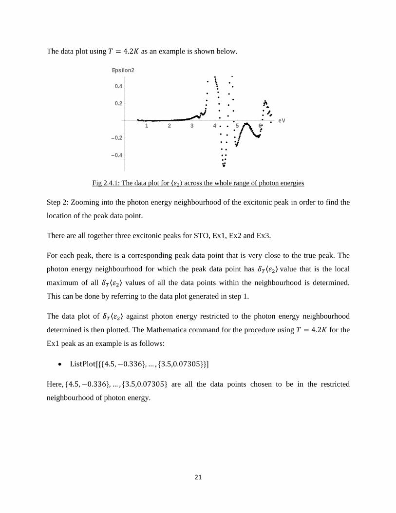
The data plot using as an example is shown below.
Fig 2.4.1: The data plot for across the whole range of photon energies
Step 2: Zooming into the photon energy neighbourhood of the excitonic peak in order to find the
location of the peak data point.
There are all together three excitonic peaks for STO, Ex1, Ex2 and Ex3.
For each peak, there is a corresponding peak data point that is very close to the true peak. The
photon energy neighbourhood for which the peak data point has value that is the local
maximum of all values of all the data points within the neighbourhood is determined.
This can be done by referring to the data plot generated in step 1.
The data plot of against photon energy restricted to the photon energy neighbourhood
determined is then plotted. The Mathematica command for the procedure using for the
Ex1 peak as an example is as follows:
Here, are all the data points chosen to be in the restricted
neighbourhood of photon energy.
1 2 3 4 5 6eV
0.4
0.2
0.2
0.4
Epsilon2
22
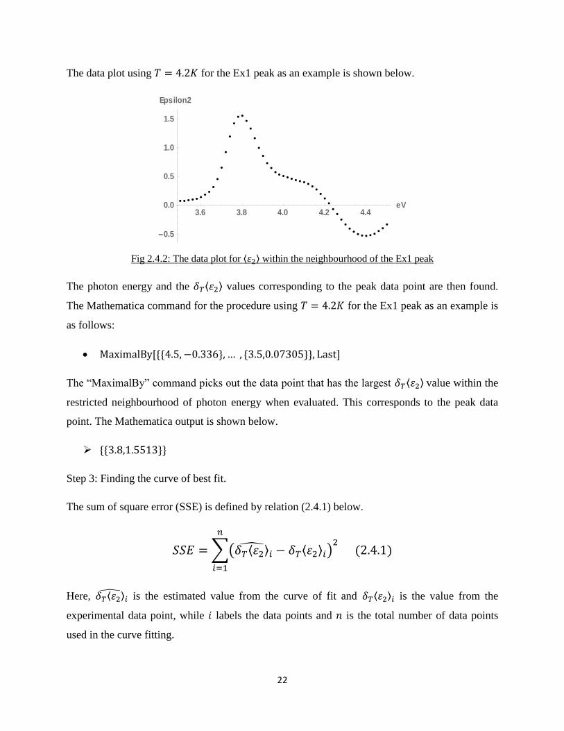
The data plot using for the Ex1 peak as an example is shown below.
Fig 2.4.2: The data plot for within the neighbourhood of the Ex1 peak
The photon energy and the values corresponding to the peak data point are then found.
The Mathematica command for the procedure using for the Ex1 peak as an example is
as follows:
The “MaximalBy” command picks out the data point that has the largest value within the
restricted neighbourhood of photon energy when evaluated. This corresponds to the peak data
point. The Mathematica output is shown below.
Step 3: Finding the curve of best fit.
The sum of square error (SSE) is defined by relation (2.4.1) below.
Here, is the estimated value from the curve of fit and is the value from the
experimental data point, while labels the data points and is the total number of data points
used in the curve fitting.
3.6 3.8 4.0 4.2 4.4eV
0.5
0.0
0.5
1.0
1.5
Epsilon2
23
The mean square error (MSE) is defined by relation (2.4.2) below.
For a particular type of curve with variable parameters, the curve of best fit is attained when the
MSE is minimized. Knowing the values of the respective parameters when the MSE is
minimized will give the equation of the curve of best fit. The process of obtaining the equation of
the curve of best fit can be split into two cases. When curve fitting any peak, we may assume
case 1. If case 1 does not suffice, then we proceed to case 2.
For each peak, we start by finding the equation of the curve of best fit for the Gaussian and
Lorentz profile respectively. We guess that the parameters and respectively take the values
of and the photon energy of the corresponding peak data point found previously in step 2.
For the parameter, we start by setting it to take the value of 0.1. Starting from the
corresponding peak data point found previously in step 2, 10 data points to its left and 10 data
points to its right are chosen. Any data points that have negative value are discarded as
these are in the invalid range of values for a Gaussian or Lorentz profile.
Next, we find the equation of the curve of best fit for the Gaussian and Lorentz profile
respectively. The Mathematica commands for the procedure using for the Ex1 peak as
an example for the Gaussian and Lorentz profile respectively are as follows:
For all the curve fittings done, it has been observed that the parameter of every curve of best fit
for the Gaussian or Lorentz profile always takes values close to 0.1. Hence, it suffices to use 0.1
as a guess for all curve fittings involving the Gaussian and Lorentz profile. Furthermore, since
the pseudo Voigt profile is a linear combination of the Gaussian and Lorentz profile, we expect
the parameter of every curve of best fit for the pseudo Voigt profile to take values close to 0.1
as well.
24
Case 1: The unconstrained pseudo Voigt profile suffices.
For each peak, we start by trying to curve fit the pseudo Voigt profile. We guess that the
parameters and respectively take the values of and the photon energy of the
corresponding peak data point found previously in step 2 and the parameter takes the value
0.1. We initially fix the parameter to take the value of 0.5. That is, assuming half Gaussian and
half Lorentz profile. Starting from the corresponding peak data point found previously in step 2,
10 data points to its left and 10 data points to its right are chosen. Any data points that have
negative value are discarded as these are in the invalid range of values for a pseudo Voigt
profile.
Next, we find the equation of the curve of best fit for a pseudo Voigt profile. The Mathematica
command for the procedure using for the Ex1 peak as an example are as follows:
Here, are all the data points chosen for the curve fitting, and a, b, c
and d are the parameters of the pseudo Voigt profile. The “FindFit” command picks out the
particular values of the parameters that give the pseudo Voigt profile with the minimum MSE
and hence gives the equation of the curve of best fit for the pseudo Voigt profile. The
Mathematica output is shown below.
Only the parameter that needs to be varied when guessed. The parameter is bounded below
by 0 and above by 1. As a rule of thumb, we can first guess the parameter to take the value of
0.5. Should unreasonable estimates of any of the parameters be obtained, we guess the
parameter again in increasing or decreasing steps of 0.1. In the case of the Ex1 peak
example, the guessed parameter values all turn out to be close to the parameter values that give
the minimum MSE and hence, a reasonable answer is obtained immediately.
25
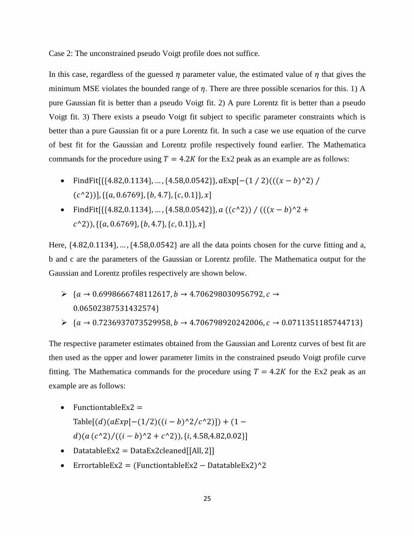
Case 2: The unconstrained pseudo Voigt profile does not suffice.
In this case, regardless of the guessed parameter value, the estimated value of that gives the
minimum MSE violates the bounded range of . There are three possible scenarios for this. 1) A
pure Gaussian fit is better than a pseudo Voigt fit. 2) A pure Lorentz fit is better than a pseudo
Voigt fit. 3) There exists a pseudo Voigt fit subject to specific parameter constraints which is
better than a pure Gaussian fit or a pure Lorentz fit. In such a case we use equation of the curve
of best fit for the Gaussian and Lorentz profile respectively found earlier. The Mathematica
commands for the procedure using for the Ex2 peak as an example are as follows:
Here, are all the data points chosen for the curve fitting and a,
b and c are the parameters of the Gaussian or Lorentz profile. The Mathematica output for the
Gaussian and Lorentz profiles respectively are shown below.
The respective parameter estimates obtained from the Gaussian and Lorentz curves of best fit are
then used as the upper and lower parameter limits in the constrained pseudo Voigt profile curve
fitting. The Mathematica commands for the procedure using for the Ex2 peak as an
example are as follows:
26
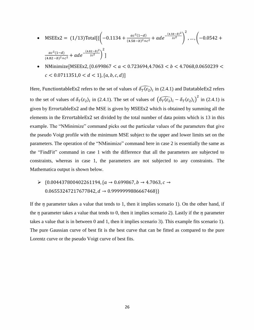
Here, refers to the set of values of in (2.4.1) and refers
to the set of values of in (2.4.1). The set of values of
in (2.4.1) is
given by and the MSE is given by which is obtained by summing all the
elements in the set divided by the total number of data points which is 13 in this
example. The “NMinimize” command picks out the particular values of the parameters that give
the pseudo Voigt profile with the minimum MSE subject to the upper and lower limits set on the
parameters. The operation of the “NMinimize” command here in case 2 is essentially the same as
the “FindFit” command in case 1 with the difference that all the parameters are subjected to
constraints, whereas in case 1, the parameters are not subjected to any constraints. The
Mathematica output is shown below.
If the parameter takes a value that tends to 1, then it implies scenario 1). On the other hand, if
the parameter takes a value that tends to 0, then it implies scenario 2). Lastly if the parameter
takes a value that is in between 0 and 1, then it implies scenario 3). This example fits scenario 1).
The pure Gaussian curve of best fit is the best curve that can be fitted as compared to the pure
Lorentz curve or the pseudo Voigt curve of best fits.
27
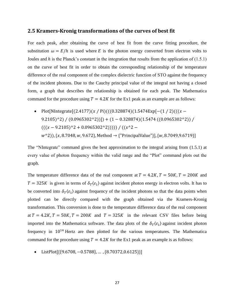
2.5 Kramers-Kronig transformations of the curves of best fit
For each peak, after obtaining the curve of best fit from the curve fitting procedure, the
substitution is used where is the photon energy converted from electron volts to
Joules and is the Planck’s constant in the integration that results from the application of (1.5.1)
on the curve of best fit in order to obtain the corresponding relationship of the temperature
difference of the real component of the complex dielectric function of STO against the frequency
of the incident photons. Due to the Cauchy principal value of the integral not having a closed
form, a graph that describes the relationship is obtained for each peak. The Mathematica
command for the procedure using for the Ex1 peak as an example are as follows:
The “NIntegrate” command gives the best approximation to the integral arising from (1.5.1) at
every value of photon frequency within the valid range and the “Plot” command plots out the
graph.
The temperature difference data of the real component at , , and
is given in terms of against incident photon energy in electron volts. It has to
be converted into against frequency of the incident photons so that the data points when
plotted can be directly compared with the graph obtained via the Kramers-Kronig
transformation. This conversion is done to the temperature difference data of the real component
at , , and in the relevant CSV files before being
imported into the Mathematica software. The data plots of the against incident photon
frequency in Hertz are then plotted for the various temperatures. The Mathematica
command for the procedure using for the Ex1 peak as an example is as follows:

28
We then compare the graph obtained for the temperature difference of the real component via the
Kramers-Kronig transformation of the fitted curve with the experimental data points for the
temperature difference of the real component.

29
Chapter 3: Results and Discussion
In this section, we will discuss the physical insight that we can gain from the curve fitting results
of the experimental data points of the temperature difference of the imaginary component of the
complex dielectric function and the results of the Kramers-Kronig transformation on the curve
fitted results. By considering the temperature difference of the imaginary component in (2.4.1),
we are assuming that interband transitions do not exist in the formation of the resonant exciton.
By performing the curve fitting and subsequently comparing the Kramers-Kronig transformation
of the best fit curve to the experimental data points of the real component of the complex
dielectric function, we should be able to tell if this assumption is valid for the resonant exciton.
3.1 The curve fitting results
The following table shows the respective curves of best fit and the corresponding excitonic peaks
in the temperature difference data of the imaginary component of the complex dielectric function
across the different temperatures.
Excitonic
Peak
Temperature Curve of
Best Fit
A
Parameter
B
Parameter
C
Parameter
D
Parameter
Ex1 4.2K Pseudo-
Voigt
1.54740 3.80914 0.0965302 0.328874
Ex2 4.2K Pure
Gaussian
0.699867 4.70630 0.0650239 -
Ex3 4.2K Pure
Gaussian
0.211112 6.24982 0.102759 -
Ex1 50K Pseudo-
Voigt
1.46836 3.81599 0.0962429 0.437108
Ex2 50K Pure
Gaussian
0.678594 4.71109 0.0641915 -
Ex3 50K Pure
Gaussian
0.175823 6.26828 0.112125 -
30
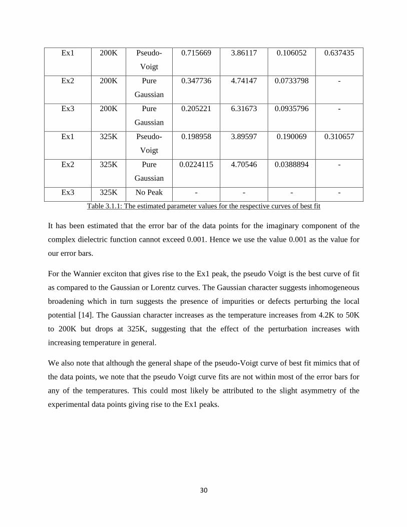
Ex1 200K Pseudo-
Voigt
0.715669 3.86117 0.106052 0.637435
Ex2 200K Pure
Gaussian
0.347736 4.74147 0.0733798 -
Ex3 200K Pure
Gaussian
0.205221 6.31673 0.0935796 -
Ex1 325K Pseudo-
Voigt
0.198958 3.89597 0.190069 0.310657
Ex2 325K Pure
Gaussian
0.0224115 4.70546 0.0388894 -
Ex3 325K No Peak - - - -
Table 3.1.1: The estimated parameter values for the respective curves of best fit
It has been estimated that the error bar of the data points for the imaginary component of the
complex dielectric function cannot exceed 0.001. Hence we use the value 0.001 as the value for
our error bars.
For the Wannier exciton that gives rise to the Ex1 peak, the pseudo Voigt is the best curve of fit
as compared to the Gaussian or Lorentz curves. The Gaussian character suggests inhomogeneous
broadening which in turn suggests the presence of impurities or defects perturbing the local
potential [14]. The Gaussian character increases as the temperature increases from 4.2K to 50K
to 200K but drops at 325K, suggesting that the effect of the perturbation increases with
increasing temperature in general.
We also note that although the general shape of the pseudo-Voigt curve of best fit mimics that of
the data points, we note that the pseudo Voigt curve fits are not within most of the error bars for
any of the temperatures. This could most likely be attributed to the slight asymmetry of the
experimental data points giving rise to the Ex1 peaks.
31
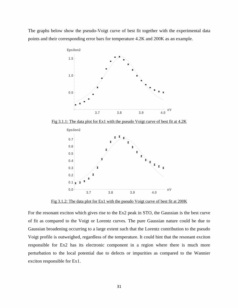
The graphs below show the pseudo-Voigt curve of best fit together with the experimental data
points and their corresponding error bars for temperature 4.2K and 200K as an example.
Fig 3.1.1: The data plot for Ex1 with the pseudo Voigt curve of best fit at 4.2K
Fig 3.1.2: The data plot for Ex1 with the pseudo Voigt curve of best fit at 200K
For the resonant exciton which gives rise to the Ex2 peak in STO, the Gaussian is the best curve
of fit as compared to the Voigt or Lorentz curves. The pure Gaussian nature could be due to
Gaussian broadening occurring to a large extent such that the Lorentz contribution to the pseudo
Voigt profile is outweighed, regardless of the temperature. It could hint that the resonant exciton
responsible for Ex2 has its electronic component in a region where there is much more
perturbation to the local potential due to defects or impurities as compared to the Wannier
exciton responsible for Ex1.
3.7 3.8 3.9 4.0eV
0.5
1.0
1.5
Epsilon2
3.7 3.8 3.9 4.0eV0.0
0.1
0.2
0.3
0.4
0.5
0.6
0.7
Epsilon2
32
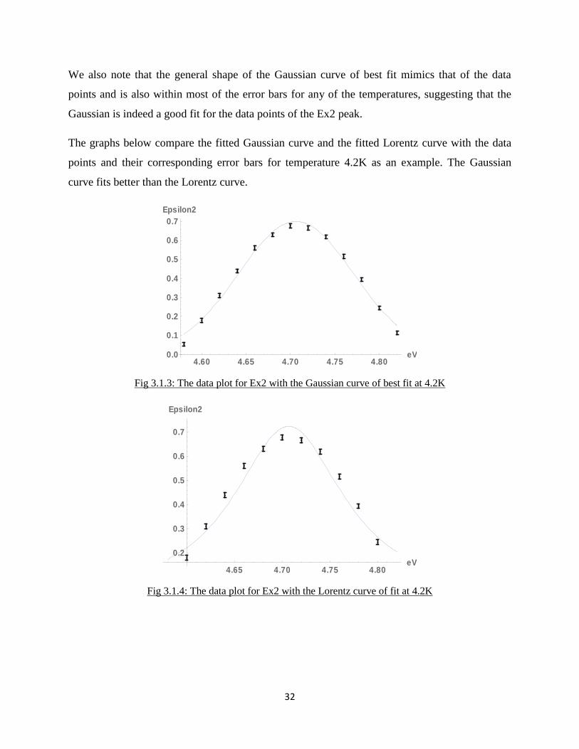
We also note that the general shape of the Gaussian curve of best fit mimics that of the data
points and is also within most of the error bars for any of the temperatures, suggesting that the
Gaussian is indeed a good fit for the data points of the Ex2 peak.
The graphs below compare the fitted Gaussian curve and the fitted Lorentz curve with the data
points and their corresponding error bars for temperature 4.2K as an example. The Gaussian
curve fits better than the Lorentz curve.
Fig 3.1.3: The data plot for Ex2 with the Gaussian curve of best fit at 4.2K
Fig 3.1.4: The data plot for Ex2 with the Lorentz curve of fit at 4.2K
4.60 4.65 4.70 4.75 4.80eV0.0
0.1
0.2
0.3
0.4
0.5
0.6
0.7
Epsilon2
4.65 4.70 4.75 4.80eV
0.2
0.3
0.4
0.5
0.6
0.7
Epsilon2
33
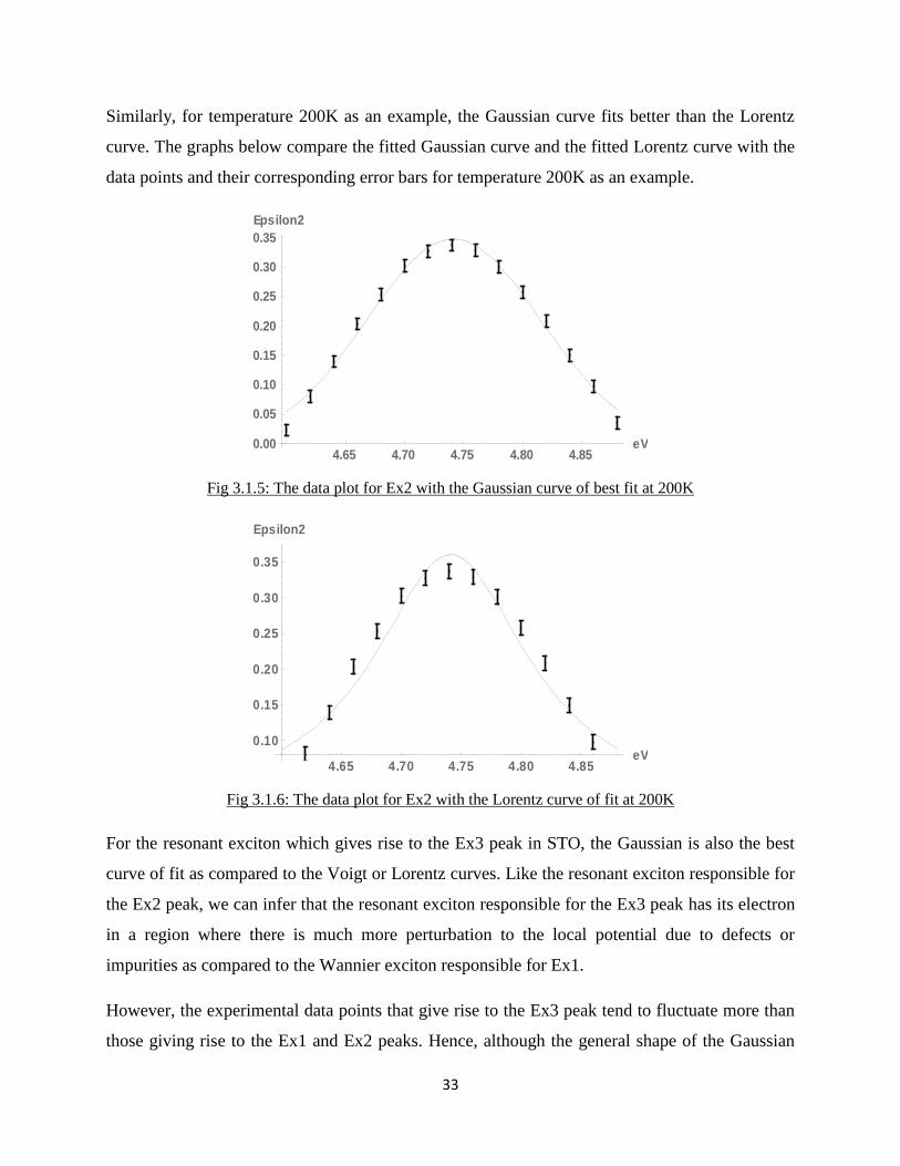
Similarly, for temperature 200K as an example, the Gaussian curve fits better than the Lorentz
curve. The graphs below compare the fitted Gaussian curve and the fitted Lorentz curve with the
data points and their corresponding error bars for temperature 200K as an example.
Fig 3.1.5: The data plot for Ex2 with the Gaussian curve of best fit at 200K
Fig 3.1.6: The data plot for Ex2 with the Lorentz curve of fit at 200K
For the resonant exciton which gives rise to the Ex3 peak in STO, the Gaussian is also the best
curve of fit as compared to the Voigt or Lorentz curves. Like the resonant exciton responsible for
the Ex2 peak, we can infer that the resonant exciton responsible for the Ex3 peak has its electron
in a region where there is much more perturbation to the local potential due to defects or
impurities as compared to the Wannier exciton responsible for Ex1.
However, the experimental data points that give rise to the Ex3 peak tend to fluctuate more than
those giving rise to the Ex1 and Ex2 peaks. Hence, although the general shape of the Gaussian
4.65 4.70 4.75 4.80 4.85eV0.00
0.05
0.10
0.15
0.20
0.25
0.30
0.35
Epsilon2
4.65 4.70 4.75 4.80 4.85eV
0.10
0.15
0.20
0.25
0.30
0.35
Epsilon2
34
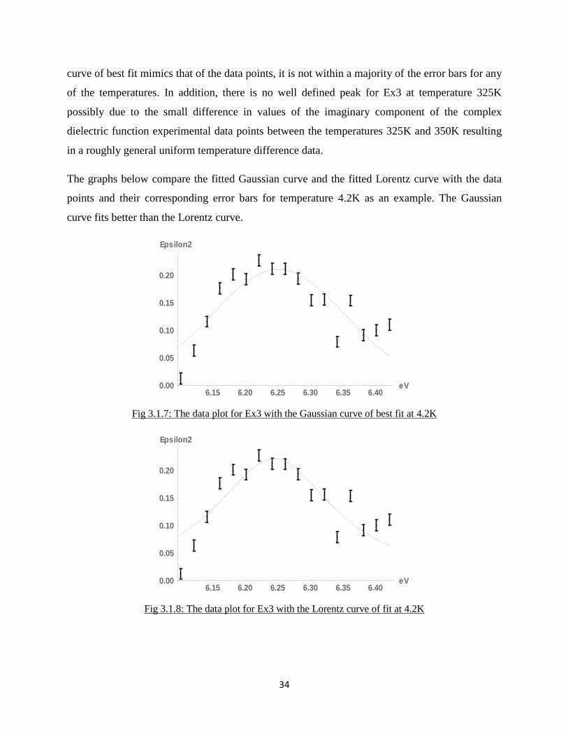
curve of best fit mimics that of the data points, it is not within a majority of the error bars for any
of the temperatures. In addition, there is no well defined peak for Ex3 at temperature 325K
possibly due to the small difference in values of the imaginary component of the complex
dielectric function experimental data points between the temperatures 325K and 350K resulting
in a roughly general uniform temperature difference data.
The graphs below compare the fitted Gaussian curve and the fitted Lorentz curve with the data
points and their corresponding error bars for temperature 4.2K as an example. The Gaussian
curve fits better than the Lorentz curve.
Fig 3.1.7: The data plot for Ex3 with the Gaussian curve of best fit at 4.2K
Fig 3.1.8: The data plot for Ex3 with the Lorentz curve of fit at 4.2K
6.15 6.20 6.25 6.30 6.35 6.40eV0.00
0.05
0.10
0.15
0.20
Epsilon2
6.15 6.20 6.25 6.30 6.35 6.40eV0.00
0.05
0.10
0.15
0.20
Epsilon2
35
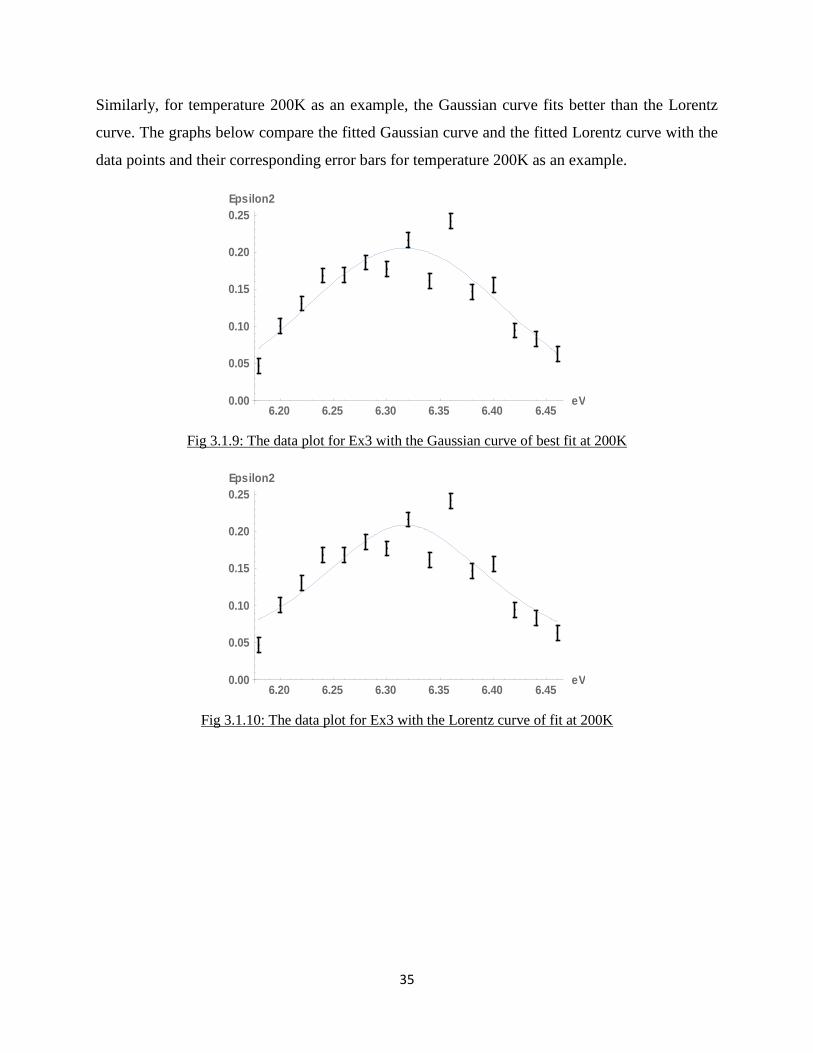
Similarly, for temperature 200K as an example, the Gaussian curve fits better than the Lorentz
curve. The graphs below compare the fitted Gaussian curve and the fitted Lorentz curve with the
data points and their corresponding error bars for temperature 200K as an example.
Fig 3.1.9: The data plot for Ex3 with the Gaussian curve of best fit at 200K
Fig 3.1.10: The data plot for Ex3 with the Lorentz curve of fit at 200K
6.20 6.25 6.30 6.35 6.40 6.45eV0.00
0.05
0.10
0.15
0.20
0.25
Epsilon2
6.20 6.25 6.30 6.35 6.40 6.45eV0.00
0.05
0.10
0.15
0.20
0.25
Epsilon2
36
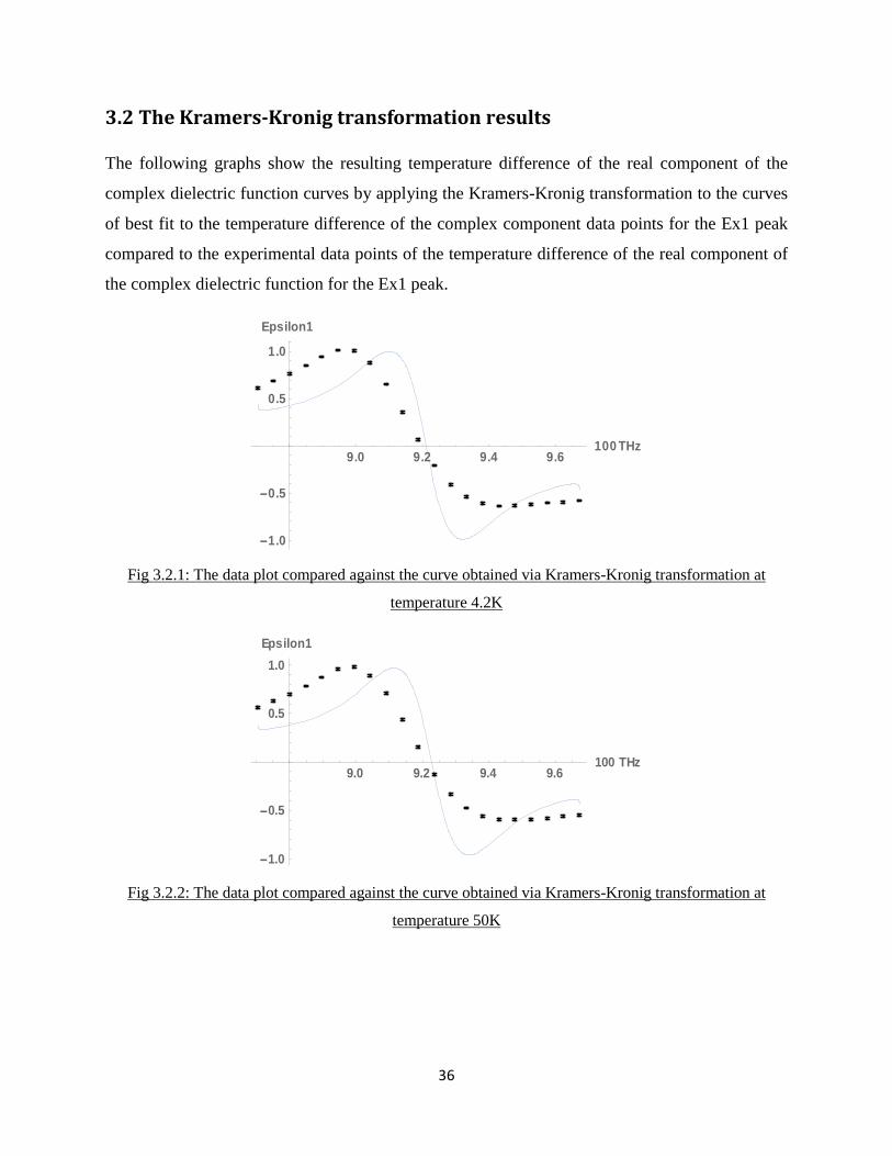
3.2 The Kramers-Kronig transformation results
The following graphs show the resulting temperature difference of the real component of the
complex dielectric function curves by applying the Kramers-Kronig transformation to the curves
of best fit to the temperature difference of the complex component data points for the Ex1 peak
compared to the experimental data points of the temperature difference of the real component of
the complex dielectric function for the Ex1 peak.
Fig 3.2.1: The data plot compared against the curve obtained via Kramers-Kronig transformation at
temperature 4.2K
Fig 3.2.2: The data plot compared against the curve obtained via Kramers-Kronig transformation at
temperature 50K
9.0 9.2 9.4 9.6100 THz
1.0
0.5
0.5
1.0
Epsilon1
9.0 9.2 9.4 9.6100 THz
1.0
0.5
0.5
1.0
Epsilon1
37
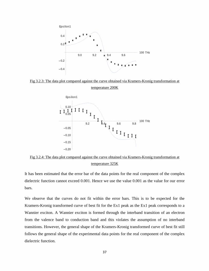
Fig 3.2.3: The data plot compared against the curve obtained via Kramers-Kronig transformation at
temperature 200K
Fig 3.2.4: The data plot compared against the curve obtained via Kramers-Kronig transformation at
temperature 325K
It has been estimated that the error bar of the data points for the real component of the complex
dielectric function cannot exceed 0.001. Hence we use the value 0.001 as the value for our error
bars.
We observe that the curves do not fit within the error bars. This is to be expected for the
Kramers-Kronig transformed curve of best fit for the Ex1 peak as the Ex1 peak corresponds to a
Wannier exciton. A Wannier exciton is formed through the interband transition of an electron
from the valence band to conduction band and this violates the assumption of no interband
transitions. However, the general shape of the Kramers-Kronig transformed curve of best fit still
follows the general shape of the experimental data points for the real component of the complex
dielectric function.
9.0 9.2 9.4 9.6100 THz
0.4
0.2
0.2
0.4
Epsilon1
9.2 9.4 9.6 9.8100 THz
0.20
0.15
0.10
0.05
0.05
0.10
Epsilon1
38
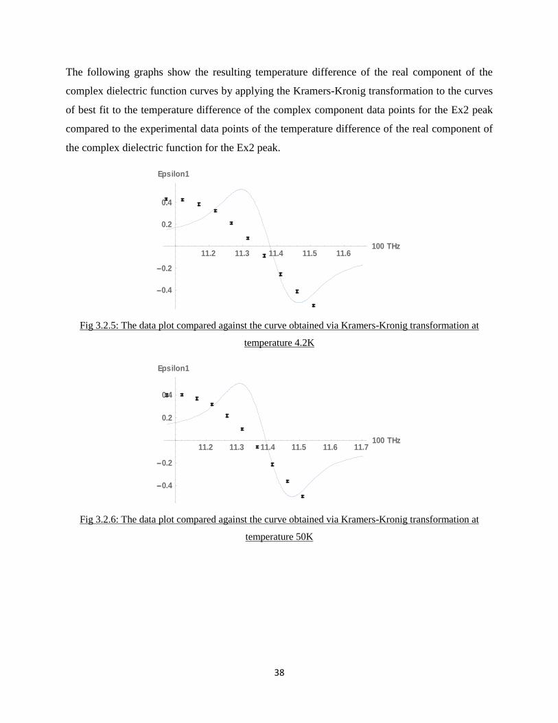
The following graphs show the resulting temperature difference of the real component of the
complex dielectric function curves by applying the Kramers-Kronig transformation to the curves
of best fit to the temperature difference of the complex component data points for the Ex2 peak
compared to the experimental data points of the temperature difference of the real component of
the complex dielectric function for the Ex2 peak.
Fig 3.2.5: The data plot compared against the curve obtained via Kramers-Kronig transformation at
temperature 4.2K
Fig 3.2.6: The data plot compared against the curve obtained via Kramers-Kronig transformation at
temperature 50K
11.2 11.3 11.4 11.5 11.6100 THz
0.4
0.2
0.2
0.4
Epsilon1
11.2 11.3 11.4 11.5 11.6 11.7100 THz
0.4
0.2
0.2
0.4
Epsilon1
39
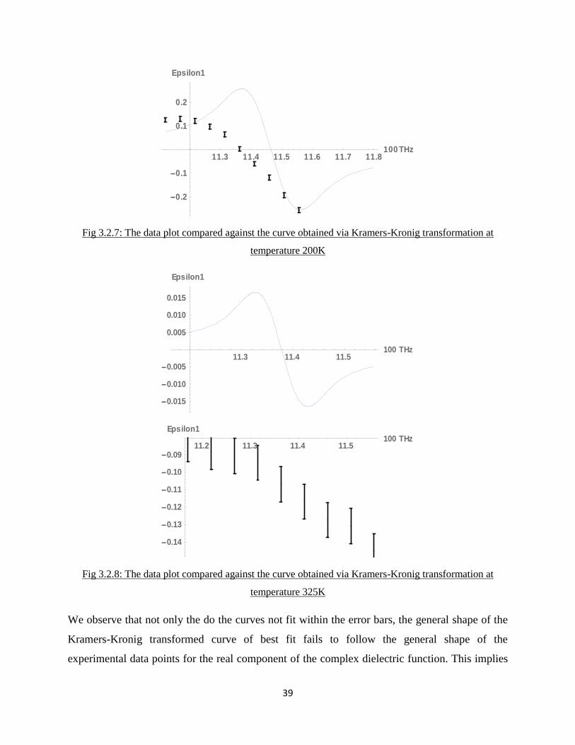
Fig 3.2.7: The data plot compared against the curve obtained via Kramers-Kronig transformation at
temperature 200K
Fig 3.2.8: The data plot compared against the curve obtained via Kramers-Kronig transformation at
temperature 325K
We observe that not only the do the curves not fit within the error bars, the general shape of the
Kramers-Kronig transformed curve of best fit fails to follow the general shape of the
experimental data points for the real component of the complex dielectric function. This implies
11.3 11.4 11.5 11.6 11.7 11.8100 THz
0.2
0.1
0.1
0.2
Epsilon1
11.3 11.4 11.5100 THz
0.015
0.010
0.005
0.005
0.010
0.015
Epsilon1
11.2 11.3 11.4 11.5100 THz
0.14
0.13
0.12
0.11
0.10
0.09
Epsilon1
40
that the assumption interband transitions do not play a role in the formation of the Ex2 resonant
exciton is not valid.
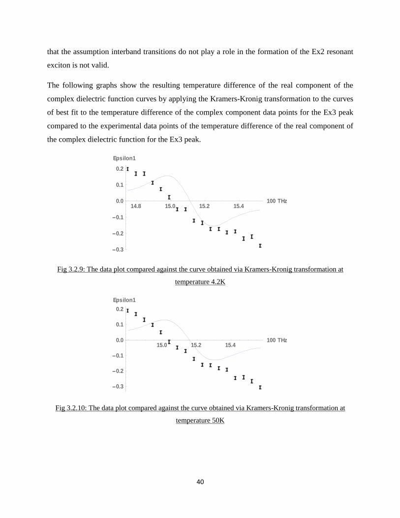
The following graphs show the resulting temperature difference of the real component of the
complex dielectric function curves by applying the Kramers-Kronig transformation to the curves
of best fit to the temperature difference of the complex component data points for the Ex3 peak
compared to the experimental data points of the temperature difference of the real component of
the complex dielectric function for the Ex3 peak.
Fig 3.2.9: The data plot compared against the curve obtained via Kramers-Kronig transformation at
temperature 4.2K
Fig 3.2.10: The data plot compared against the curve obtained via Kramers-Kronig transformation at
temperature 50K
14.8 15.0 15.2 15.4100 THz
0.3
0.2
0.1
0.0
0.1
0.2
Epsilon1
15.0 15.2 15.4100 THz
0.3
0.2
0.1
0.0
0.1
0.2
Epsilon1
41
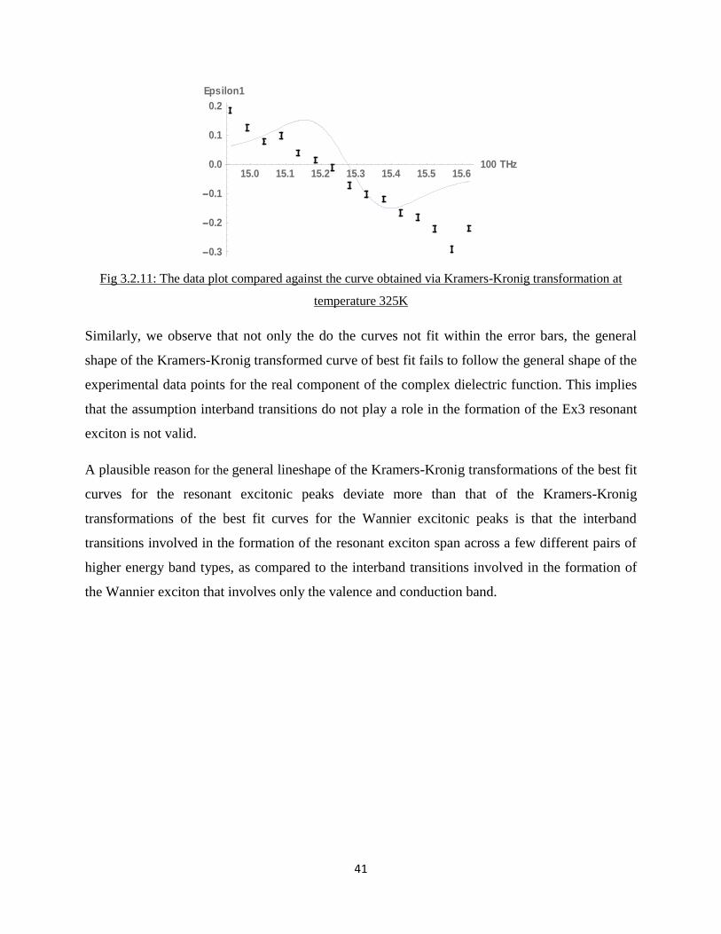
Fig 3.2.11: The data plot compared against the curve obtained via Kramers-Kronig transformation at
temperature 325K
Similarly, we observe that not only the do the curves not fit within the error bars, the general
shape of the Kramers-Kronig transformed curve of best fit fails to follow the general shape of the
experimental data points for the real component of the complex dielectric function. This implies
that the assumption interband transitions do not play a role in the formation of the Ex3 resonant
exciton is not valid.
A plausible reason for the general lineshape of the Kramers-Kronig transformations of the best fit
curves for the resonant excitonic peaks deviate more than that of the Kramers-Kronig
transformations of the best fit curves for the Wannier excitonic peaks is that the interband
transitions involved in the formation of the resonant exciton span across a few different pairs of
higher energy band types, as compared to the interband transitions involved in the formation of
the Wannier exciton that involves only the valence and conduction band.
15.0 15.1 15.2 15.3 15.4 15.5 15.6100 THz
0.3
0.2
0.1
0.0
0.1
0.2
Epsilon1

42
Chapter 4: Conclusion & Future Work
4.1 Conclusion
The Ex1, Ex2 and Ex3 excitonic peaks of the temperature difference of the imaginary component
of the complex dielectric function were curve fitted with well known bell-shaped profiles based
on the least mean square error criterion. All the curve-fitted peaks displayed a Gaussian character
which implies the presence of impurities or defects in the STO sample leading to inhomogeneous
broadening, with the resonant excitons experiencing greater perturbation than the Wannier
excitons.
The Kramers-Kronig transformations of the best fit curves of the peaks do not fit within error
bars of the data points of the temperature difference of the real component of the complex
dielectric function. This implies that like the Ex1 Wannier exciton, interband transitions exist in
the formation of the Ex2 and Ex3 resonant excitons. In addition the general lineshape of the
Kramers-Kronig transformations of the best fit curves for the excitonic peaks deviate from the
general lineshape of the data points of the temperature difference of the real component of the
complex dielectric function for the Ex2 and Ex3 resonant excitons. While for the Ex1 Wannier
exciton, the general lineshape of the Kramers-Kronig transformations of the best fit curves for
the excitonic peaks mimic the general lineshape of the data points of the temperature difference
of the real component of the complex dielectric function. This implies that while interband
transitions between the valence and conduction bands can give rise to the Ex1 Wannier exciton,
interband transitions involving several pairs of higher energy bands can give rise to the Ex2 and
Ex3 resonant excitons.

43
4.2 Future work
There is a slight asymmetry in the Ex1 Wannier excitonic peak for the imaginary component of
the complex dielectric function data points. Hence, an asymmetric pseudo Voigt profile which
has to take into account many body effects multi-electron excitations in the sample [15] might
be considered in future curve fitting purposes.
As the Gaussian character in all the curve fittings seem to suggest the presence of impurities or
defects in the sample being used, future experiments may be carried out on STO samples with
known levels of doping to check if indeed the level of Gaussian character in the new curve
fittings increase with the level of doping.
The data points towards higher photon energies also tend to fluctuate more making it more
difficult to do curve fitting. Future spectroscopic ellipsometry experiments could consider taking
a few repeated runs and taking the average of the readings corresponding to each reading of
photon energy for photon energies that are within the neighborhood of the Ex3 peak.
Finally, we should seek the higher energy bands responsible for the interband transitions that are
responsible for the formation of the Ex2 and Ex3 resonant excitons in STO in future research.
44
References
[1] Hewitt, Paul G, 2006, Conceptual Physics, San Francisco: Pearson Addison Wesley.
[2] Halliday, D., Resnick, R., and Walker, J., 2008, Fundamentals of physics (8th ed.), Hoboken, NJ:
Wiley.
[3] Huray, Paul G, 2010, Maxwell’s Equations, Wiley-Blackwell.
[4] Mannan Ali, 1999, Growth and study of magnetostrictive FeSiBC thin films, for device applications
[5] Griffiths, 2014, Introduction to Electrodynamics 4th edition-Electromagnetic Waves, Pearson.
[6] Martin Pope and Charles E Swenberg, 1999, Electronic Processes in Organic Crystals and Polymers
2nd
edition, Oxford University Press
[7] Z. Yong, P.E. Trevisanutto, L. Chiodo, I. Santoso, A.R. Barman, T.C. Asmara, S. Dhar, A. Kotlov, A.
Terentjevs, F. Della Sala, V. Olevano, M. Rubhausen, T. Venkatesan and A. Rusydi, Phy. Rev. B93,
205118 (2016)
[8] Fujiwara, 2007, Spectroscopic Ellipsometry: Principles and Applications, John Wiley & Sons, Ltd
[9] T. Leisegang, H. Stöcker, A. A. Levin, T. Weißbach, M. Zschornak, E. Gutmann, K. Rickers, S.
Gemming, and D. C. Meyer, Phy. Rev. Lett102,087601 (2008)
[10] Prócel, L. M., Tipán, F., & Stashans, A. (2003). Mott–Wannier excitons in the tetragonal BaTiO3
lattice. International Journal of Quantum Chemistry, 91(4), 586590. doi:10.1002/qua.10471
[11] F.M.F. De Groot, M. Grioni, J.C. Fuggle, J. Ghijsen, G.A. Sawatzky and H. Petersen, Phys. Rev. B
40 (1989), pp. 5715–5723.
[12] P.K. Gogoi, L. Sponza, D. Schmidt, T.C. Asmara, C. Diao, J.C.W. Lim, S.M. Poh, S. Kimura, P.E.
Trevisanutto, V.Olevano and A. Rusydi, Phy. Rev. B92,035119 (2015)
[13] Bales, B. L., Peric, M., & LamyFreund, M. T. (1998). Contributions to the gaussian line broadening
of the proxyl spin probe EPR spectrum due to magneticfield modulation and unresolved proton hyperfine
structure. Journal of Magnetic Resonance, 132(2), 279286. doi:10.1006/jmre.1998.1414
[14] P.K. Gogoi, Z. Hu, Q. Wang, A. Carvalho, D. Schmidt, X. Yin, Y. H. Chang, L.J. Li, C.H. Sow,
A.H.C. Neto, M.B.H. Breese, A. Rusydi and A.T.S. Wee (2017) .Oxygen Passivation Mediated
Turnability of Trion and Excitons in MoS2.
[15] Schmid, M., Steinrück, H., & Gottfried, J. M. (2014). A new asymmetric pseudovoigt function for
more efficient fitting of XPS lines: New asymmetric pseudovoigt function for efficient XPS line fitting.
Surface and Interface Analysis, 46(8), 505511. doi:10.1002/sia.5521


![Influence of Annealing Temperatures on the Structural, Morphological… · 2020. 1. 29. · greatly affected by its growth routes [9]. Strontium titanate (SrTiO 3) perovskite material](https://img.dokumen.tips/doc/110x75/60b88a1c38582264692512f9/influence-of-annealing-temperatures-on-the-structural-morphological-2020-1-29.jpg)
![D. Rama Krishna Sharma*, Dr P. Vijay Bhaskar Rao** · ... Barium Strontium Cobalt Iron Titanate{Ba 0 ... deficiency of oxygen & x is various compositions ], powders ... SOL-GEL method](https://img.dokumen.tips/doc/110x75/5b87fe497f8b9a435b8ce39b/d-rama-krishna-sharma-dr-p-vijay-bhaskar-rao-barium-strontium-cobalt.jpg)