RESEARCH OpenAccess Experimentalevaluationofthe ... · RESEARCH OpenAccess Experimentalevaluationofthe ... of an experimental investigation of 2 × 2 MIMO-OFDM channel measurements

Onubogu et al. EURASIP Journal onWireless Communications andNetworking (2015) 2015:183 DOI 10.1186/s13638-015-0411-5

RESEARCH Open Access

Experimental evaluation of theperformance of 2 × 2MIMO-OFDM forvehicle-to-infrastructure communicationsOkechukwu J. Onubogu1*, Karla Ziri-Castro1, Dhammika Jayalath1 and Hajime Suzuki2

Abstract

In this paper, a novel 2 × 2 multiple-input multiple-output orthogonal frequency division multiplexing (MIMO-OFDM)testbed based on an Analog Devices AD9361 highly integrated radio frequency (RF) agile transceiver was specificallyimplemented for the purpose of estimating and analyzing MIMO-OFDM channel capacity in vehicle-to-infrastructure(V2I) environments using the 920 MHz industrial, scientific, and medical (ISM) band. We implementedtwo-dimensional discrete cosine transform-based filtering to reduce the channel estimation errors and show itseffectiveness on our measurement results. We have also analyzed the effects of channel estimation error on the MIMOchannel capacity by simulation. Three different scenarios of subcarrier spacing were investigated which correspond toIEEE 802.11p, Long-Term Evolution (LTE), and Digital Video Broadcasting Terrestrial (DVB-T)(2k) standards. An extensiveMIMO-OFDM V2I channel measurement campaign was performed in a suburban environment. Analysis of themeasured MIMO channel capacity results as a function of the transmitter-to-receiver (TX-RX) separation distance up to250 m shows that the variance of the MIMO channel capacity is larger for the near-range line-of-sight (LOS) scenariosthan for the long-range non-LOS cases, using a fixed receiver signal-to-noise ratio (SNR) criterion. We observed thatthe largest capacity values were achieved at LOS propagation despite the common assumption of a degeneratedMIMO channel in LOS. We consider that this is due to the large angular spacing between MIMO subchannels whichoccurs when the receiver vehicle rooftop antennas pass by the fixed transmitter antennas at close range, causingMIMO subchannels to be orthogonal. In addition, analysis on the effects of different subcarrier spacings onMIMO-OFDM channel capacity showed negligible differences in mean channel capacity for the subcarrier spacingrange investigated. Measured channels described in this paper are available on request.

Keywords: MIMO-OFDM; Capacity; V2I; LOS; Channel

1 Review1.1 IntroductionMultiple-input multiple-output (MIMO) systems haveattracted considerable attention due to the increasingrequirements of high capacity, spectral efficiency, and reli-ability in wireless communications. For example, MIMOsystems have been adopted in the Long-Term Evolution(LTE) system, and it is expected that the upcoming devel-opments in IEEE 802.11p and Digital Video Broadcast-ing Terrestrial (DVB-T) wireless standards will includethe use of MIMO. It has been shown [1] that MIMO,

*Correspondence: [email protected] of Electrical Engineering and Computer Science, QueenslandUniversity of Technology, Brisbane, QLD 4001, AustraliaFull list of author information is available at the end of the article

when deployed in a rich scattering environment, is capa-ble of achieving high spectral efficiency, capacity, andreliability by exploiting the increased spatial degrees offreedom. MIMO is often combined with the orthogonalfrequency division multiplexing (OFDM) in modern wire-less standards in order to achieve higher data rates andperformance improvements in a multipath fading envi-ronment without increasing the required bandwidth ortransmission power.Efficient vehicular communication is a key in the devel-

opment of intelligent transport systems (ITS) and requiresthe exchange of messages between two vehicles (vehicle-to-vehicle or V2V communications) or between a vehicleand a roadside unit (vehicle-to-infrastructure or V2I com-

© 2015 Onubogu et al. This is an Open Access article distributed under the terms of the Creative Commons Attribution License(http://creativecommons.org/licenses/by/4.0), which permits unrestricted use, distribution, and reproduction in any medium,provided the original work is properly credited.

http://crossmark.crossref.org/dialog/?doi=10.1186/s13638-015-0411-5-x&domain=pdf

mailto: [email protected]

http://creativecommons.org/licenses/by/4.0

Onubogu et al. EURASIP Journal onWireless Communications and Networking (2015) 2015:183 Page 2 of 19

munications). Basically, there are two kinds of vehicularapplications: those dedicated to providing safety servicesand others for non-safety applications [2]. For safety pur-poses, the use of licensed band at 5.9 GHz has beenconsidered to avoid the problem of interference typicallyfaced in the use of industrial, scientific, and medical (ISM)radio bands. Non-safety applications use the ISM bandfor the purpose of infotainment (e.g., high data rate Inter-net access for video streaming) where the availability ofthe service is expected to be opportunistic. The 920 MHzISM band in Australia occupies 918–926 MHz. Amongthe ISM bands, the 920 MHz band gives an optimal trade-off of robustness against slow fading, achieving a longerrange in cluttered environments and having a sufficientbandwidth for the high-data-rate Internet access. Thispaper focuses on the non-safety V2I applications at the920 MHz ISM band which promises to provide infotain-ment applications, mobile internet services, and socialnetwork applications which are widely used in people’sdaily activities in vehicles. The successful deployment ofcommercial MIMO systems will require a solid under-standing of the channel characteristics in which it willoperate. In order to assess the performance of new wire-less communication systems using MIMO antennas, itis desirable to evaluate them in realistic measurementscenarios. Consequently, numerous MIMO channel mea-surement campaigns have been carried out in vehicularenvironments [3–7]. However, only a few research pub-lications have considered MIMO V2V channels [8–12],and even fewer theoretically based research works haveinvestigated MIMO V2I channels [13, 14]. A number ofsingle-input single-output (SISO) antenna V2V and V2Ichannel measurement campaigns have been conducted[15, 16]. However, to the best of our knowledge, we arenot aware of any MIMO-OFDM measurement results forV2I communications published in the scientific literatureto date. In this paper, we focus on presenting the resultsof an experimental investigation of 2 × 2 MIMO-OFDMchannel measurements performed in a real V2I drivingscenario under both line-of-sight (LOS) and non-LOS(NLOS) conditions at the 920 MHz ISM band in a subur-ban environment. A channel sounding system based on asoftware-defined radio (SDR) platform was implementedand used to perform an extensive measurement campaignin a suburban environment. In comparison to the useof the conventional heavy and expensive radio frequency(RF) test equipment such as signal generators, vector net-work analyzers, and spectrum analyzers, SDR providesa flexible, inexpensive, and cost-effective measurementsetup implemented in software that enables researchersto use and control the radio signal through software toolssuch as MATLAB.The rapid development of MIMO systems has been

based on the assumption that independent and identically

distributed (i.i.d) or correlated Rayleigh fading with NLOScomponents is available and a high number of multipathcomponents are created by the surrounding environment[17–19]. This, however, is not valid in all cases, and it isviolated due to the existence of a LOS component thatis stronger than other components. Hence, the channelcan be more effectively modeled using the Ricean distri-bution. Conventionally, the presence of a LOS componentis thought to limit the benefits of MIMO systems becauseof the rank deficiency of the channel matrix [20, 21];however, a number of investigations [13, 14, 22–26] haveshown that using antennas positioned or spaced in sucha way that the LOS MIMO subchannels are orthogonalresults in a full-rank MIMO channel matrix and thereforehigh-capacity channels. The common idea behind theseapproaches is to place the antenna elements sufficientlyfar apart so that the spatial LOS MIMO subchannelsbecome orthogonal with a phase difference of π/2. Theoptimal spacings can be worked out via simple geometri-cal tools, while the channel matrix becomes full rank anddelivers equal eigenvalues. This is known as an optimizedLOS MIMO system [24]. We can determine the requiredinter-element spacings to achieve the maximum 2 × 2MIMO capacity. The formula is a function of the inter-element distance, the transmitter-to-receiver (TX-RX)separation distance, the orientation of the arrays, and thecarrier frequency.This paper validates the theoretical maximum LOS

MIMO capacity criteria in [14, 25, 27, 28] by presentinga measurement-based analysis of mean MIMO capacity(mean over the channel bandwidth and the time of 50 ms)as a function of TX-RX separation distance. The tech-nique is based on the achievement of spatial multiplexingin scenarios by creating an artificial multipath not causedby physical objects but rather by deliberate antenna place-ment or separation of the antenna elements in such away that a deterministic and constant orthogonal multi-path is created at a specific TX-RX separation distancecalled Dopt. This paper also analyzes the MIMO channelcapacity for three different subcarrier spacings: large sub-carrier spacing (LSS), medium subcarrier spacing (MSS),and small subcarrier spacing (SSS). These subcarrier spac-ings approximately correspond to IEEE 802.11p WirelessAccess in Vehicular Environment, LTE, and the 2k ver-sion of the DVB-T standard. It is important to note thatthis paper analyzes the capacity of the MIMO channelswith three different values of subcarrier spacing and notthe capacity of the whole system. In this analysis, theMIMO channels are estimated by the least square (LS)channel estimation method with known channel trainingsymbols [29]. The channel estimation error due to lowersignal-to-noise ratio (SNR) at a longer TX-RX separationdistance is substantially reduced by applying two-dimensional discrete cosine transform (2D DCT)-based


filtering to take advantage of the time and frequencycoherence of the channel [30–32].The remainder of the paper is organized as follows.

Section 1.2 describes the channel model, MIMO chan-nel capacity, the derivation for maximum LOS MIMOchannel capacity criteria, and the LS channel estimation.Section 1.3 presents theMIMO-OFDMV2Imeasurementequipment, measurement environment, and parameters.In Section 1.4, we present the analysis of measurementresults. Finally, Section 2 summarizes the paper and addsconcluding remarks.

1.2 Channel model and capacity1.2.1 LOSMIMO channel modelTo investigate the capacity of aMIMO channel in the pres-ence of a LOS component, a suitable channel model forthe MIMO channel is needed. According to [21, 28] and[25], a suitable way to model the channel matrix is as asum of two components, a LOS component and a NLOScomponent. The ratio between the power of the two com-ponents gives the Ricean K factor. The MIMO channelmatrix is modeled as

H =√

KK + 1

HLOS +√

1K + 1

HNLOS (1)

where HLOS denotes the matrix containing the free spaceresponses between all elements, HNLOS accounts for thescattered signals, and K is the Ricean K-factor which isequal to the ratio of the free space and scattered signals[33, 34]. As given in [25] and [27], the free space com-ponent, HLOS, of the complex response between a trans-mitting element m and a receiving element n (assumingthat both elements are isotropic) is given as e−jβdn,m/dn,mwhere β is the wave number corresponding to the car-rier wavelength λ and it is given as β = 2π

λ. dn,m is the

distance between the nth receiving element and the mthtransmitting element. With the assumption that the dif-ference in the pathloss is negligible and that there is nomutual coupling between the elements, the normalizedfree space response matrix of an nr × nt MIMO systemcan be expressed as

HLOS =

⎡⎢⎢⎢⎣

e−jβd1,1 e−jβd1,2 . . . e−jβd1,nt

e−jβd2,1 e−jβd2,2 . . . e−jβd2,nt...

......

. . .e−jβdnr ,1 e−jβdnr ,2 . . . e−jβdnr ,nt

⎤⎥⎥⎥⎦

where HLOS is totally deterministic and depends only onthe positioning or separation distance between both ele-ments of the RX and TX antennas. Contrastingly, theresponse due to HNLOS is a random complex matrix and isoften modeled by stochastic process, i.e., HNLOS ε ⊂nr×nt

with i.i.d elements.

1.2.2 MIMO channel capacityIn any communication system, the fundamental measureof performance is the capacity of the channel, which isthe maximum rate of communication for which arbitrar-ily small error probability can be achieved [35]. In thissection, the capacity definition of MIMO systems is pre-sented and the minimum and maximum capacity criteriaare derived in terms of the channel response matrix. Inthis case, the receiver is assumed to have perfect chan-nel state information (CSI) but no such prior knowledge isavailable at the transmitter. Hence, the Shannon capacityformula for the MIMO channel is given as [1, 36]

Ck = log2(det

(Inr + ρ

ntHkHH

k

))(2)

whereCk is theMIMO channel capacity in bits per secondper Hertz (bits/s/Hz) at the kth OFDM subcarrier, Inr isthe identitymatrix and superscriptH denotes the complexconjugate transpose (Hermitian), ρ corresponds to theaverage received SNR per receiver over MIMO subchan-nels, and nt and nr are the number of transmitting andreceiving antenna elements, respectively. We note that theabove capacity formula relies on a uniform power alloca-tion scheme at all transmitting elements. Assuming thatnt ≤ nr , we can write

Ck =nt∑

m=1log2

(1 + ρ

ntγm(Hk)

)(3)

where γm(Hk) is the mth eigenvalue of HkHHk . The maxi-

mum capacity is achieved when the channel is orthogonal[1], for which HkHH

k is a diagonal matrix with ||Hk,m||2Fas its (m,m)-th element, where ||Hk,m||2F is the squaredFrobenius norm of the mth row of Hk . In this case,γm(Hk) = ||Hk,m||2F . The MIMO channel capacity iscalculated at each OFDM subcarrier using the aboveequation, while the MIMO-OFDM channel capacity iscalculated as an average of the MIMO channel capacityover all OFDM subcarriers at a fixed signal SNR= 20 dB.For our measurement analysis, we chose signal SNR=20 dB to have an even estimation of the MIMO channelcapacity along the path and to emphasize effects of theMIMO channel structure on the capacity. The fixed valueof signal SNR= 20 dB was chosen as an example, whichis typically used for MIMO channel capacity analysis forthe system using 16-quadrature amplitude modulation(QAM) or 64-QAM (e.g., [27, 37])We note that the MIMO capacity value monotonically

increases or decreases with the higher or lower signalSNR and it does not affect the conclusions of compara-tive analysis of higher or lower MIMO channel capacityas a function of subcarrier spacing or environment ashave been performed in this paper. The MIMO chan-nel capacity referred to in this paper corresponds to an


ideal capacity, where it is assumed that a perfect CSI isavailable at the receiver. The actual capacity is typicallyreduced from this capacity due to the inaccuracy of theCSI at the receiver, especially in a mobile environment. Inaddition, the effects of inter-carrier interference (ICI) andinter-symbol interference (ISI) are ignored in this paper.We consider that the effects of ICI are small given thesubcarrier spacing used and the maximum Doppler shiftassumed. The ISI is expected to be removed by the use ofcyclic prefix.For a SISO fading channel with perfect knowledge of the

channel at the receiver, the capacity of a SISO link is givenas C = log2(1 + ρ). Therefore, the capacity of an equiv-alent SISO link is equal to approximately 6.66 bps/Hz atρ.In this paper, there are two types of SNR being dis-

cussed. The first is nominated as ρ in (2) and is referredas signal SNR. The second SNR is referred to as channelestimation (CE) SNR which indicates the quality of thechannel estimation.

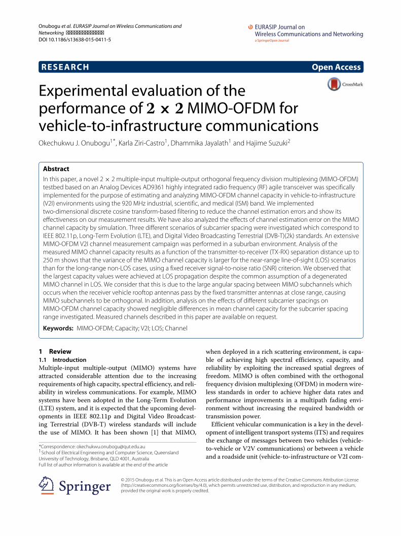
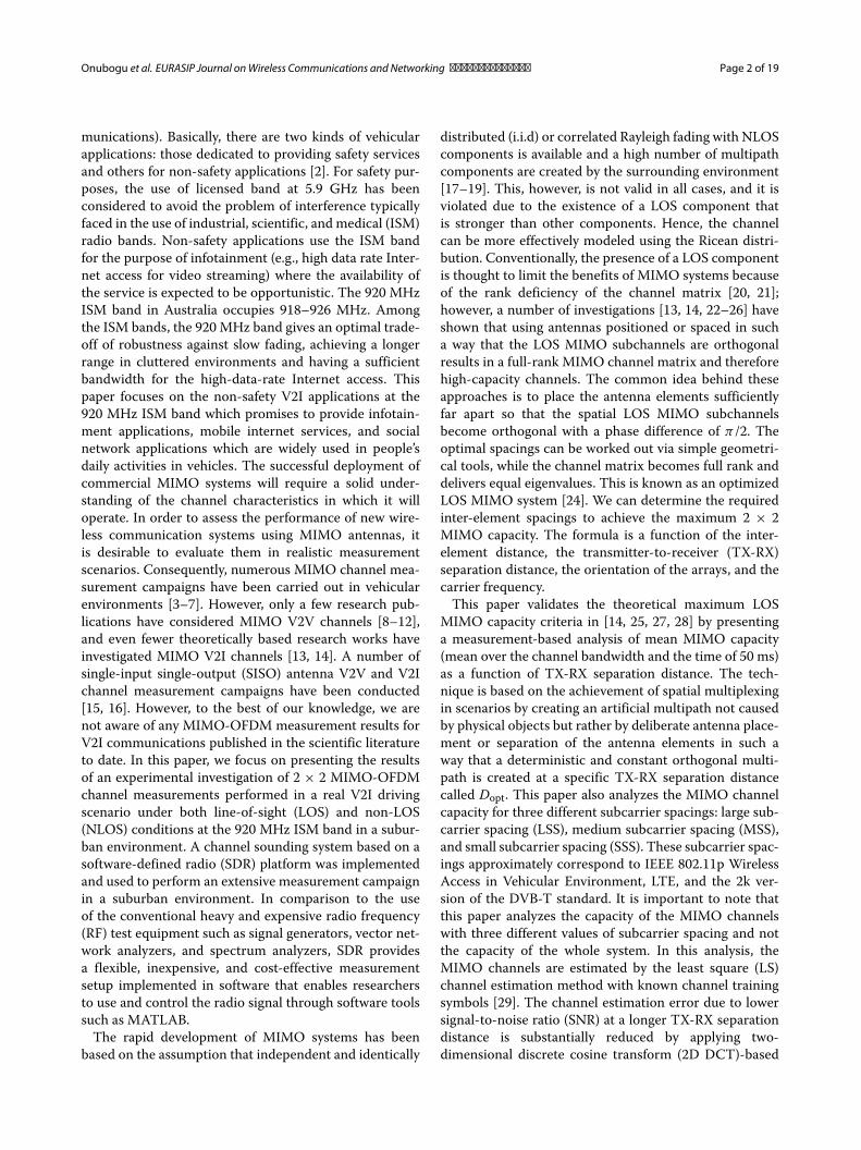
1.2.3 Maximum LOSMIMO capacity criteriaIn conventionalMIMO systems, an inter-element antennaspacing equal to λ/2 is considered to be adequate toavoid strong correlation between received signals [38]. Formost indoor applications, this inter-element spacing is stillapplicable; however, for V2I systems, such spacing cannotbe used to achieve maximum capacity due to the largerdistance between RX and TX, which tends to reduce theangular spacing and hence to increase correlation betweensubchannels. Figure 1 shows an example of the geometryof the positions of TX and RX antenna elements and asso-ciated parameters in V2I systems. In Fig. 1, θ is the angularspacing between the two MIMO subchannels. We used a2 × 2 MIMO system as the basis of our derivation of themaximum capacity criterion. Figure 2 shows a simplified2D version of the model.The conditions for achieving the minimum and maxi-

mum capacities in a time-invariant or slow time-varyingMIMO channel are given below as in [27]. The minimumMIMO capacity is obtained when HHH = nt1nr , where1nr is an nr × nr all ones matrix. This corresponds toa system with rank-1 HLOS response with an associatedcapacity that is equivalent to that of a SISO channel givenas Cmin = log2(1 + nrρ). The capacity in Eq. (2) is maxi-mized for HHH = ntInr , i.e., when H is orthogonal. Thisresponse corresponds to a system with perfectly orthog-onal MIMO subchannels, and the capacity of the MIMOchannel is then equivalent to that of nr independent SISOchannels given as follows: Cmax = nr log2(1 + ρ), Cmaxcorresponds to amaximum capacity value of 13.32 bps/Hzfor a 2×2MIMO system. From the normalized free spacechannel response matrix of the nr × nt MIMO systemgiven above, the correlation matrix is given as follows:

Fig. 1 Positions of TX and RX antenna elements with the RX vehicle(OBU antennas) mounted at the rooftop of a car moving along astreet in x and y directions while the TX roadside unit (RSU antennas)was mounted at a fixed position

HHH =⎡⎢⎣

nt . . .∑nt

m=1 e−jβ(d1,m−dnr ,m)

.... . .

...∑ntm=1 e−jβ(dnr ,m−d1,m) . . . nr

⎤⎥⎦

In the case of the 2 × 2 MIMO system, the aboveequation can be simplified to

HHH =[

2 ejβ(d21−d11) + ejβ(d22−d12)

ejβ(d11−d21) + ejβ(d12−d22) 2

]

It is clearly seen that the matrices are deterministicand depend on the distance between the TX and RX ele-ments [39]. It can be seen that HHH becomes a square

Fig. 2 A 2 × 2 MIMO near-range LOS system with parallel arrays


matrix in which all the elements of the principal diag-onal are twos and all other elements are zeros whenejβ(d11−d21) + ejβ(d12−d22) = 0. Based on the mathematicalconditions given in the previous paragraph, it is clear thatthe maximum capacity of a 2× 2 MIMO is achieved when

HHH = ntInr = 2I2, (4)

that is, when all eigenvalues ofHHH become equal and weend up with perfectly orthogonal MIMO spatial subchan-nels. Sarris et al. in [25, 27] have shown that this maximumcapacity condition is satisfied when

|d11 − d12 + d22 − d21| = (2r + 1)λ

2, rεZ+ (5)

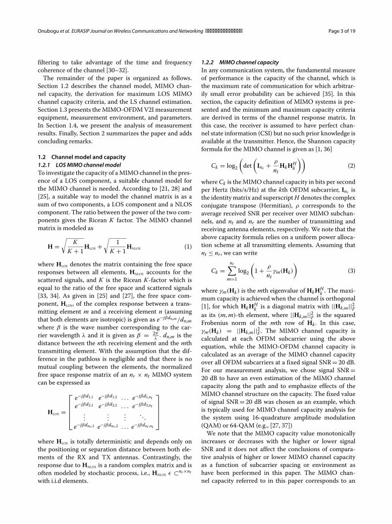
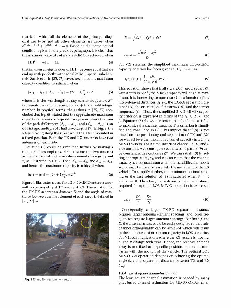
where λ is the wavelength at any carrier frequency, Z+represents the set of integers, and (2r+1) is an odd integernumber. In physical terms, the authors in [25, 27] con-cluded that Eq. (5) stated that the approximate maximumcapacity criterion corresponds to systems where the sumof the path differences (d11 − d12) and (d22 − d21) is anodd integermultiple of a half wavelength [27]. In Fig. 3, theRX is moving along the street while the TX is mounted ina fixed position. Both the TX and RX antennas have twoantennas on each side.Equation (5) could be simplified further by making a

number of assumptions. First, assume the two antennaarrays are parallel and have inter-element spacings, s1 ands2 as illustrated in Fig. 2. Then, d11 = d22 and d12 = d21,and hence, the maximum capacity is achieved when

|d11 − d21| = (2r + 1)λ

4, rεZ+ (6)

Figure 1 illustrates a case for a 2× 2 MIMO antenna arraywith a spacing of s1 at TX and s2 at RX. The equation forthe TX-RX separation distance D and the angle of rota-tion θ between the first element of each array is defined in[25, 27] as

Fig. 3 TX and RX measurement setup

D =√dx2 + dy2 + dz2 (7)

cos θ =√dx2 + dy2

D(8)

For V2I systems, the simplified maximum LOS-MIMOcapacity criterion has been given in [13, 14, 25] as

s1s2 ≈ (r + 12)

Dλ

cos2 θ, rεZ+ (9)

This equation shows that if all s1, s2, D, θ , and λ satisfy (9)with a certain rεZ+, theMIMO capacity will be at its max-imum. It is interesting to note that (9) is a function of theinter-element distances (s1, s2), the TX-RX separation dis-tance (D), the orientation of the arrays (θ), and the carrierfrequency (fc). Thus, the simplified 2 × 2 MIMO capac-ity criterion is expressed in terms of the s1, s2, D, θ , andfc. Equation (5) shows a criterion that should be satisfiedto maximize the channel capacity. The criterion is simpli-fied and concluded in (9). This implies that if (9) is metbased on the positioning and separation of TX and RX,we will achieve the maximum channel capacity in a 2 × 2MIMO system. For a time-invariant channel, λ, D, and θ

are constant. As a consequence, the second part of (9) canbe constant with a certain rεZ+. We can satisfy (9) by set-ting appropriate s1, s2, and we can claim that the channelcapacity is at its maximumwhen that is fulfilled. In mobilescenarios,D and θ may vary with the movement of the RXvehicle. To simplify further, the minimum optimal spac-ing or the first solution of (9) is satisfied when θ = 0and r = 0. Therefore, the antenna separation distancerequired for optimal LOS MIMO operation is expressedas

s1s2 = Dλ

2= Dc

2f(10)

Conceptually, a larger TX-RX separation distancerequires larger antenna element spacings, and lower fre-quencies require larger antenna spacings. For fixed f andD, the antenna arrays could be easily designed so that sub-channel orthogonality can be achieved which will resultto the attainment of maximum capacity in LOS scenarios.For V2I communications where the RX vehicle is moving,D and θ change with time. Hence, the receiver antennaarray is not fixed at a specific position, but its locationvaries with the motion of the vehicle. The optimal LOSMIMO V2I operation depends on achieving the optimalangle θopt and separation distance between TX and RXDopt.

1.2.4 Least square channel estimationThe least square channel estimation is needed by manypilot-based channel estimation for MIMO-OFDM as an


initial estimation. It is the simplest approach to pilot-symbol-aided (PSA) channel estimation in OFDM sys-tems, and no a priori information is assumed to be knownabout the statistics of the channel taps. However, it showspoor accuracy as it is performed on a frame-by-framebasis with no filtering of the estimate. The SISO-OFDMsystem model at the nth OFDM symbol and kth OFDMsubcarrier is given as [29]

Yn,k = Xn,kHn,k + Wn,k (11)

Yn,k is the received signals, Xn,k is the transmitted signal,and Wn,k is the adaptive white Gaussian noise (AWGN).The LS channel estimation HLSn,k is given as

HLSn,k = Yn,kXn,k

= Hn,k + Wn,kXn,k

(12)

It is important to note that this simple LS estimate HLS

does not exploit the correlation of channels across fre-quency carriers and across OFDM symbols. We utilizedthe LS estimation approach to get the initial MIMO chan-nel estimates at the pilot subcarriers, which was thenfurther improved using a 2D DCT filtering technique inboth time and frequency [30–32]. The effectiveness of thistechnique is shown in the Section 1.4.

1.3 MIMO-OFDM V2I measurements1.3.1 Measurement equipmentThe 2×2MIMO-OFDMV2I channel measurements wereperformed using an in-house built software-defined radioplatform using AD9361 dual MIMO RF agile transceiversfrom Analog Devices, as TX and RX. The AD9361is a wideband 2 × 2 MIMO transceiver. It combinesan RF front-end with a flexible mixed-signal basebandsection with a 12-bit analog-to-digital converter (ADC)and a digital-to-analog converter (DAC) and integratedfrequency synthesizers. It provides a configurable digi-tal interface to a processor. It operates from 70 MHzto 6.0 GHz, with tunable bandwidth from 200 kHz to56 MHz. The equipment transmits channel soundingOFDM signals with three different subcarrier spacings, asshown in Table 1.A custom-built user interface software running onWin-

dows operating system was used. This software capturesADC samples and records them on a PC’s hard disk viaUSB connection. The transmitter sends OFDM signals tosound the channel, which are eventually recorded at thereceiver unit. By post-processing, we then obtained thecomplex channel transfer function or frequency responseas explained in Section 1.2.4. The transmitted OFDM sig-nal waveforms (DAC samples) were generated off-line inthe PC, using MATLAB. The in-house built platform isequipped with a field-programmable gate array (FPGA)that streams the off-line generated waveforms to theAD9361’s DAC. The baseband-to-RF module amplifies,

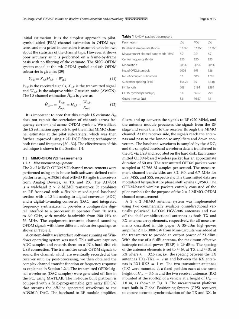
Table 1 OFDM packet parameters

Parameters LSS MSS SSS

Baseband sample rate (Msps) 32.768 32.768 32.768

Measurement channel bandwidth (MHz) 8.2 9.0 6.7

Center frequency (MHz) 920 920 920

Modulation QPSK QPSK QPSK

No. of OFDM symbols 6003 593 156

No. of occupied subcarriers 52 600 1705

Subcarrier spacing (kHz) 156.25 15 3.348

FFT length 208 2184 8384

OFDM symbol period (μs) 6.4 66.67 299

Guard interval (μs) 1.6 16.67 75

filters, and up-converts the signals to RF (920 MHz), andthe antenna module processes the signals from the RFstage and sends them to the receiver through the MIMOchannel. At the receiver side, the signals reach the anten-nas and pass to the low-noise amplifiers and down con-verters. The baseband waveform is sampled by the ADC,and the sampled baseband waveform data is transferred tothe PC via USB and recorded on the hard disk. Each trans-mitted OFDM-based wireless packet has an approximateduration of 50 ms. The transmitted OFDM packets weresampled at 32.768 M samples per second. The measure-ment channel bandwidths are 8.2, 9.0, and 6.7 MHz forLSS, MSS, and SSS, respectively. The transmitted data aremodulated by quadrature phase shift keying (QPSK). TheOFDM-based wireless packets entirely consisted of thepilot symbols for the purpose of the 2 × 2 MIMO-OFDMchannel measurement.A 2 × 2 MIMO antenna system was implemented

using two commercially available omnidirectional ver-tically polarized L-COM HGV-906 antennas and twooff-the-shelf omnidirectional antennas as both TX andRX antenna array elements, respectively, for all measure-ments described in this paper. A 35-dBm high-poweramplifier ZHL-1000-3W fromMini-Circuits was added atthe transmitter to provide an output power of 23 dBm.With the use of a 6-dBi antenna, the maximum effectiveisotropic radiated power (EIRP) is 29 dBm. The spacingof the antenna elements is set to ≈ 6λ at TX and ≈ 3λ atRX where λ = 32.5 cm, i.e., the spacing between the TXantennas TX1-TX2 = 2 m and between the RX anten-nas is RX1-RX2 = 1 m. The two transmitter antennas(TX) were mounted at a fixed position each at the sameheight of HTX = 3.6 m and the two receiver antennas (RX)mounted at the rooftop of a vehicle at a height of HRX =1.8 m, as shown in Fig. 3. The measurement platformuses built-in Global Positioning System (GPS) receiversto ensure accurate synchronization of the TX and RX. In


addition, the receiver system was equipped with an exter-nal EVK-6T-0 U-blox 6 GPS to provide measurement timestamp as well as the location and speed data for the RXvehicle.We used a portable Rohde & Schwarz (R&S) FSH8 spec-

trum analyzer to measure the interference from otherdevices operating at the 920 MHz band. We observedthat the transmitted signal from a nearby cellular basestation was causing desensitization of our receiver. As asolution, we used channel filters to remove the effects ofthe interfering signals during the measurements. No othersignificant interference in the 920 MHz ISM band wasobserved during the measurements. All the measurementequipment was separately calibrated with Agilent signalgenerators and signal analyzers. The TX output powerwas measured with a power meter. The measurementparameters are summarized in Table 2.

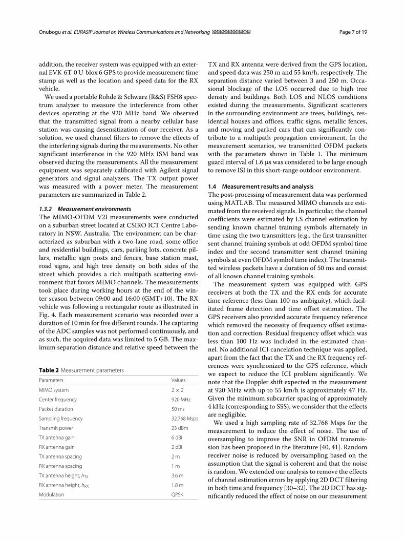
1.3.2 Measurement environmentsThe MIMO-OFDM V2I measurements were conductedon a suburban street located at CSIRO ICT Centre Labo-ratory in NSW, Australia. The environment can be char-acterized as suburban with a two-lane road, some officeand residential buildings, cars, parking lots, concrete pil-lars, metallic sign posts and fences, base station mast,road signs, and high tree density on both sides of thestreet which provides a rich multipath scattering envi-ronment that favors MIMO channels. The measurementstook place during working hours at the end of the win-ter season between 09:00 and 16:00 (GMT+10). The RXvehicle was following a rectangular route as illustrated inFig. 4. Each measurement scenario was recorded over aduration of 10min for five different rounds. The capturingof the ADC samples was not performed continuously, andas such, the acquired data was limited to 5 GB. The max-imum separation distance and relative speed between the

Table 2 Measurement parameters

Parameters Values

MIMO system 2 × 2

Center frequency 920 MHz

Packet duration 50 ms

Sampling frequency 32.768 Msps

Transmit power 23 dBm

TX antenna gain 6 dBi

RX antenna gain 2 dBi

TX antenna spacing 2 m

RX antenna spacing 1 m

TX antenna height, hTX 3.6 m

RX antenna height, hRX 1.8 m

Modulation QPSK

TX and RX antenna were derived from the GPS location,and speed data was 250 m and 55 km/h, respectively. Theseparation distance varied between 3 and 250 m. Occa-sional blockage of the LOS occurred due to high treedensity and buildings. Both LOS and NLOS conditionsexisted during the measurements. Significant scatterersin the surrounding environment are trees, buildings, res-idential houses and offices, traffic signs, metallic fences,and moving and parked cars that can significantly con-tribute to a multipath propagation environment. In themeasurement scenarios, we transmitted OFDM packetswith the parameters shown in Table 1. The minimumguard interval of 1.6 μs was considered to be large enoughto remove ISI in this short-range outdoor environment.

1.4 Measurement results and analysisThe post-processing of measurement data was performedusing MATLAB. The measured MIMO channels are esti-mated from the received signals. In particular, the channelcoefficients were estimated by LS channel estimation bysending known channel training symbols alternately intime using the two transmitters (e.g., the first transmittersent channel training symbols at odd OFDM symbol timeindex and the second transmitter sent channel trainingsymbols at evenOFDM symbol time index). The transmit-ted wireless packets have a duration of 50 ms and consistof all known channel training symbols.The measurement system was equipped with GPS

receivers at both the TX and the RX ends for accuratetime reference (less than 100 ns ambiguity), which facil-itated frame detection and time offset estimation. TheGPS receivers also provided accurate frequency referencewhich removed the necessity of frequency offset estima-tion and correction. Residual frequency offset which wasless than 100 Hz was included in the estimated chan-nel. No additional ICI cancelation technique was applied,apart from the fact that the TX and the RX frequency ref-erences were synchronized to the GPS reference, whichwe expect to reduce the ICI problem significantly. Wenote that the Doppler shift expected in the measurementat 920 MHz with up to 55 km/h is approximately 47 Hz.Given the minimum subcarrier spacing of approximately4 kHz (corresponding to SSS), we consider that the effectsare negligible.We used a high sampling rate of 32.768 Msps for the

measurement to reduce the effect of noise. The use ofoversampling to improve the SNR in OFDM transmis-sion has been proposed in the literature [40, 41]. Randomreceiver noise is reduced by oversampling based on theassumption that the signal is coherent and that the noiseis random.We extended our analysis to remove the effectsof channel estimation errors by applying 2D DCT filteringin both time and frequency [30–32]. The 2D DCT has sig-nificantly reduced the effect of noise on our measurement


Fig. 4 Google Earth map view of the measured location data from the GPS showing the location of the TX and RX route round the measurementenvironment. The blue line shows the route taken by RX, and and yellow dot shows the fixed location of TX. The indicated driving route outside roadsare considered to be due to errors in estimating locations

results. In addition, we have included a simulation anal-ysis to show that the effects of channel estimation erroron MIMO channel capacity are small for high SNR up to20 dB.

1.4.1 Effects of channel estimation error onMIMO channelcapacity

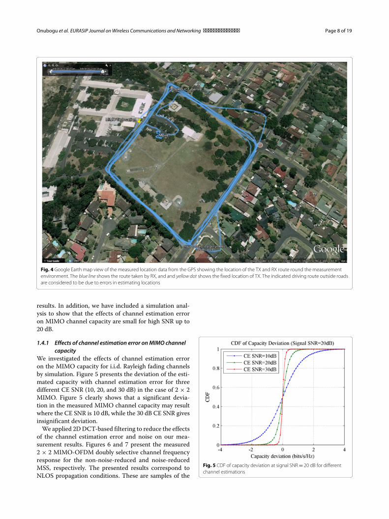
We investigated the effects of channel estimation erroron the MIMO capacity for i.i.d. Rayleigh fading channelsby simulation. Figure 5 presents the deviation of the esti-mated capacity with channel estimation error for threedifferent CE SNR (10, 20, and 30 dB) in the case of 2 × 2MIMO. Figure 5 clearly shows that a significant devia-tion in the measured MIMO channel capacity may resultwhere the CE SNR is 10 dB, while the 30 dB CE SNR givesinsignificant deviation.We applied 2DDCT-based filtering to reduce the effects

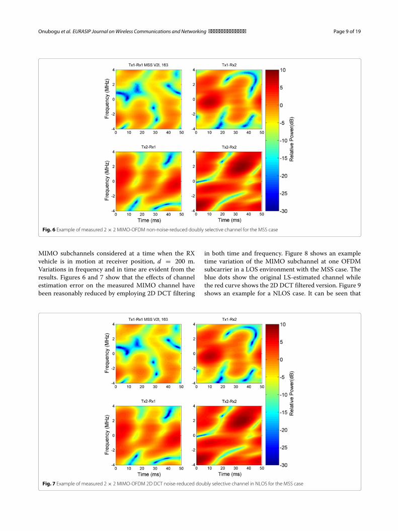
of the channel estimation error and noise on our mea-surement results. Figures 6 and 7 present the measured2 × 2 MIMO-OFDM doubly selective channel frequencyresponse for the non-noise-reduced and noise-reducedMSS, respectively. The presented results correspond toNLOS propagation conditions. These are samples of the

Fig. 5 CDF of capacity deviation at signal SNR= 20 dB for differentchannel estimations


Fig. 6 Example of measured 2 × 2 MIMO-OFDM non-noise-reduced doubly selective channel for the MSS case

MIMO subchannels considered at a time when the RXvehicle is in motion at receiver position, d = 200 m.Variations in frequency and in time are evident from theresults. Figures 6 and 7 show that the effects of channelestimation error on the measured MIMO channel havebeen reasonably reduced by employing 2D DCT filtering

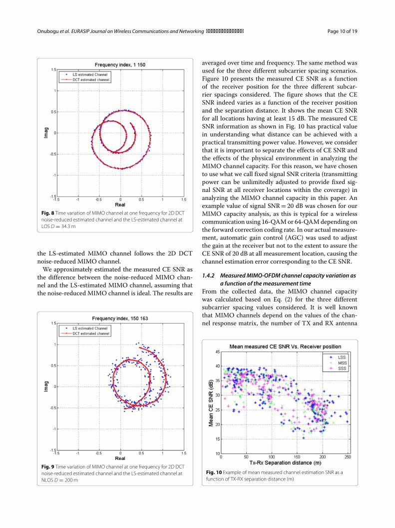
in both time and frequency. Figure 8 shows an exampletime variation of the MIMO subchannel at one OFDMsubcarrier in a LOS environment with the MSS case. Theblue dots show the original LS-estimated channel whilethe red curve shows the 2D DCT filtered version. Figure 9shows an example for a NLOS case. It can be seen that

Fig. 7 Example of measured 2 × 2 MIMO-OFDM 2D DCT noise-reduced doubly selective channel in NLOS for the MSS case


Fig. 8 Time variation of MIMO channel at one frequency for 2D DCTnoise-reduced estimated channel and the LS-estimated channel atLOS D = 34.3 m

the LS-estimated MIMO channel follows the 2D DCTnoise-reduced MIMO channel.We approximately estimated the measured CE SNR as

the difference between the noise-reduced MIMO chan-nel and the LS-estimated MIMO channel, assuming thatthe noise-reduced MIMO channel is ideal. The results are

Fig. 9 Time variation of MIMO channel at one frequency for 2D DCTnoise-reduced estimated channel and the LS-estimated channel atNLOS D = 200 m

averaged over time and frequency. The same method wasused for the three different subcarrier spacing scenarios.Figure 10 presents the measured CE SNR as a functionof the receiver position for the three different subcar-rier spacings considered. The figure shows that the CESNR indeed varies as a function of the receiver positionand the separation distance. It shows the mean CE SNRfor all locations having at least 15 dB. The measured CESNR information as shown in Fig. 10 has practical valuein understanding what distance can be achieved with apractical transmitting power value. However, we considerthat it is important to separate the effects of CE SNR andthe effects of the physical environment in analyzing theMIMO channel capacity. For this reason, we have chosento use what we call fixed signal SNR criteria (transmittingpower can be unlimitedly adjusted to provide fixed sig-nal SNR at all receiver locations within the coverage) inanalyzing the MIMO channel capacity in this paper. Anexample value of signal SNR= 20 dB was chosen for ourMIMO capacity analysis, as this is typical for a wirelesscommunication using 16-QAMor 64-QAMdepending onthe forward correction coding rate. In our actual measure-ment, automatic gain control (AGC) was used to adjustthe gain at the receiver but not to the extent to assure theCE SNR of 20 dB at all measurement location, causing thechannel estimation error corresponding to the CE SNR.

1.4.2 MeasuredMIMO-OFDM channel capacity variation asa function of themeasurement time

From the collected data, the MIMO channel capacitywas calculated based on Eq. (2) for the three differentsubcarrier spacing values considered. It is well knownthat MIMO channels depend on the values of the chan-nel response matrix, the number of TX and RX antenna

Fig. 10 Example of mean measured channel estimation SNR as afunction of TX-RX separation distance (m)


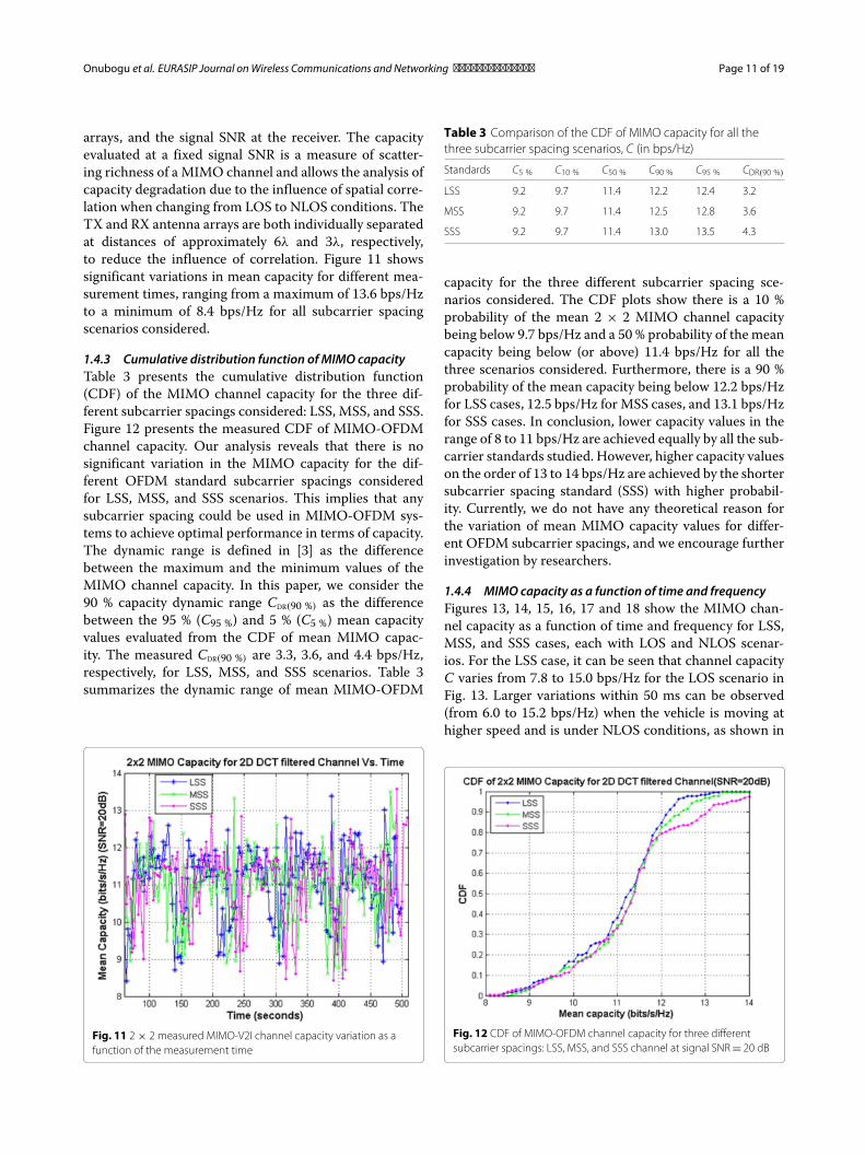
arrays, and the signal SNR at the receiver. The capacityevaluated at a fixed signal SNR is a measure of scatter-ing richness of a MIMO channel and allows the analysis ofcapacity degradation due to the influence of spatial corre-lation when changing from LOS to NLOS conditions. TheTX and RX antenna arrays are both individually separatedat distances of approximately 6λ and 3λ, respectively,to reduce the influence of correlation. Figure 11 showssignificant variations in mean capacity for different mea-surement times, ranging from a maximum of 13.6 bps/Hzto a minimum of 8.4 bps/Hz for all subcarrier spacingscenarios considered.

1.4.3 Cumulative distribution function of MIMO capacityTable 3 presents the cumulative distribution function(CDF) of the MIMO channel capacity for the three dif-ferent subcarrier spacings considered: LSS, MSS, and SSS.Figure 12 presents the measured CDF of MIMO-OFDMchannel capacity. Our analysis reveals that there is nosignificant variation in the MIMO capacity for the dif-ferent OFDM standard subcarrier spacings consideredfor LSS, MSS, and SSS scenarios. This implies that anysubcarrier spacing could be used in MIMO-OFDM sys-tems to achieve optimal performance in terms of capacity.The dynamic range is defined in [3] as the differencebetween the maximum and the minimum values of theMIMO channel capacity. In this paper, we consider the90 % capacity dynamic range CDR(90 %) as the differencebetween the 95 % (C95 %) and 5 % (C5 %) mean capacityvalues evaluated from the CDF of mean MIMO capac-ity. The measured CDR(90 %) are 3.3, 3.6, and 4.4 bps/Hz,respectively, for LSS, MSS, and SSS scenarios. Table 3summarizes the dynamic range of mean MIMO-OFDM

Fig. 11 2 × 2 measured MIMO-V2I channel capacity variation as afunction of the measurement time

Table 3 Comparison of the CDF of MIMO capacity for all thethree subcarrier spacing scenarios, C (in bps/Hz)

Standards C5 % C10 % C50 % C90 % C95 % CDR(90 %)

LSS 9.2 9.7 11.4 12.2 12.4 3.2

MSS 9.2 9.7 11.4 12.5 12.8 3.6

SSS 9.2 9.7 11.4 13.0 13.5 4.3

capacity for the three different subcarrier spacing sce-narios considered. The CDF plots show there is a 10 %probability of the mean 2 × 2 MIMO channel capacitybeing below 9.7 bps/Hz and a 50 % probability of the meancapacity being below (or above) 11.4 bps/Hz for all thethree scenarios considered. Furthermore, there is a 90 %probability of the mean capacity being below 12.2 bps/Hzfor LSS cases, 12.5 bps/Hz for MSS cases, and 13.1 bps/Hzfor SSS cases. In conclusion, lower capacity values in therange of 8 to 11 bps/Hz are achieved equally by all the sub-carrier standards studied. However, higher capacity valueson the order of 13 to 14 bps/Hz are achieved by the shortersubcarrier spacing standard (SSS) with higher probabil-ity. Currently, we do not have any theoretical reason forthe variation of mean MIMO capacity values for differ-ent OFDM subcarrier spacings, and we encourage furtherinvestigation by researchers.

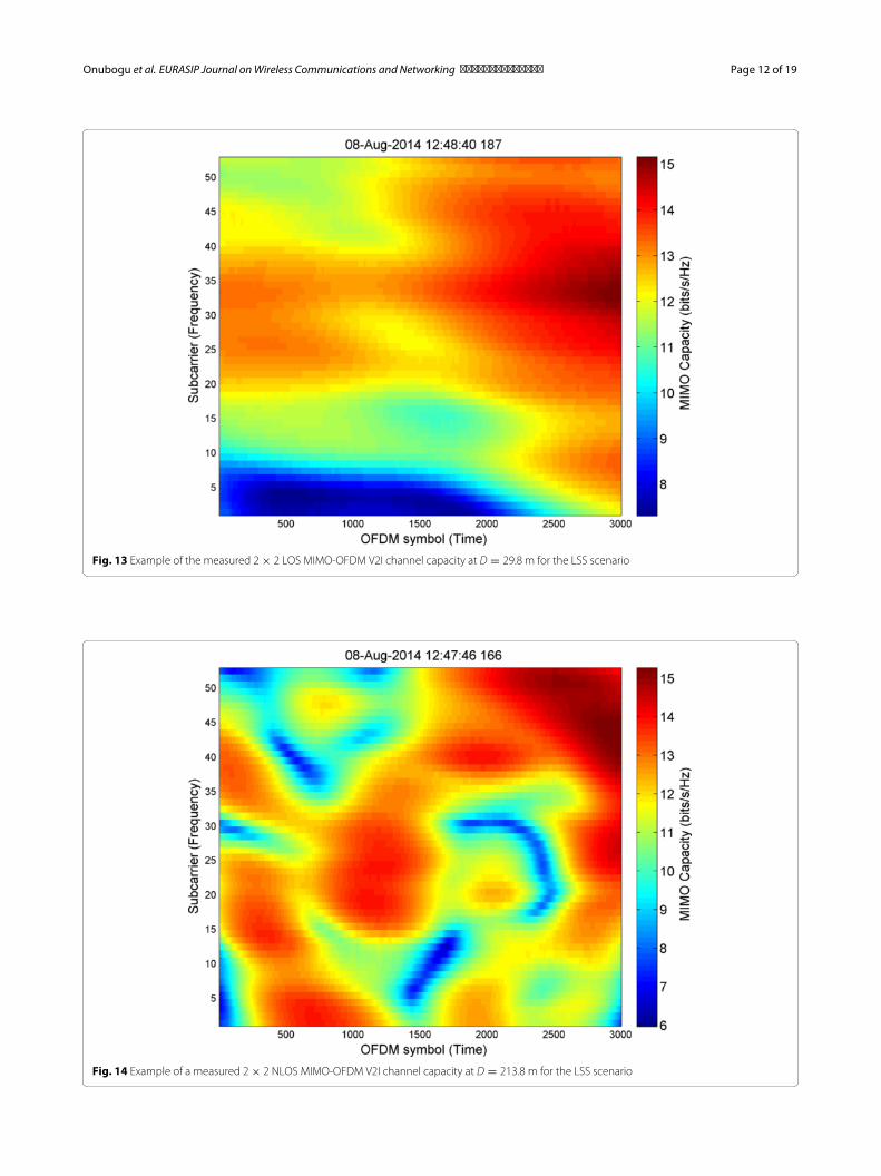
1.4.4 MIMO capacity as a function of time and frequencyFigures 13, 14, 15, 16, 17 and 18 show the MIMO chan-nel capacity as a function of time and frequency for LSS,MSS, and SSS cases, each with LOS and NLOS scenar-ios. For the LSS case, it can be seen that channel capacityC varies from 7.8 to 15.0 bps/Hz for the LOS scenario inFig. 13. Larger variations within 50 ms can be observed(from 6.0 to 15.2 bps/Hz) when the vehicle is moving athigher speed and is under NLOS conditions, as shown in

Fig. 12 CDF of MIMO-OFDM channel capacity for three differentsubcarrier spacings: LSS, MSS, and SSS channel at signal SNR= 20 dB


Fig. 13 Example of the measured 2 × 2 LOS MIMO-OFDM V2I channel capacity at D = 29.8 m for the LSS scenario

Fig. 14 Example of a measured 2 × 2 NLOS MIMO-OFDM V2I channel capacity at D = 213.8 m for the LSS scenario


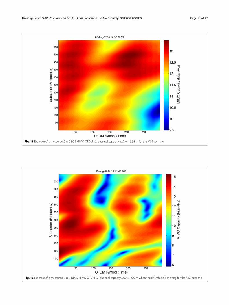
Fig. 15 Example of a measured 2 × 2 LOS MIMO-OFDM V2I channel capacity at D = 19.98 m for the MSS scenario

Fig. 16 Example of a measured 2 × 2 NLOS MIMO-OFDM V2I channel capacity at D = 200 m when the RX vehicle is moving for the MSS scenario


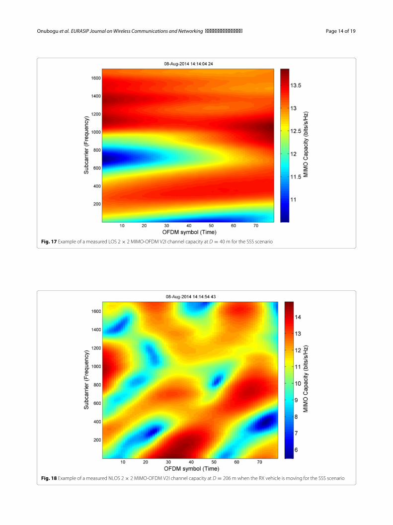
Fig. 17 Example of a measured LOS 2 × 2 MIMO-OFDM V2I channel capacity at D = 40 m for the SSS scenario

Fig. 18 Example of a measured NLOS 2 × 2 MIMO-OFDM V2I channel capacity at D = 206 m when the RX vehicle is moving for the SSS scenario


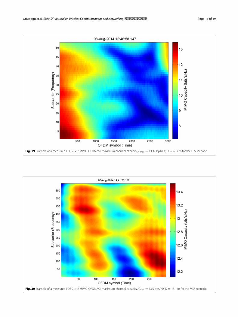
Fig. 19 Example of a measured LOS 2 × 2 MIMO-OFDM V2I maximum channel capacity, Cmax = 13.37 bps/Hz, D = 76.7 m for the LSS scenario

Fig. 20 Example of a measured LOS 2 × 2 MIMO-OFDM V2I maximum channel capacity, Cmax ≈ 13.0 bps/Hz, D = 13.1 m for the MSS scenario


Fig. 14. For the MSS case, the capacity varies from 9.5 to13.5 bps/Hz for LOS in Fig. 15 and from 6.0 to 15 bps/Hzfor NLOS scenario in Fig. 16. And for the SSS case, thecapacity varies from 10.5 to 14.0 bps/Hz and from 5.5 to15.0 bps/Hz for LOS and NLOS scenarios, respectively.Generally, greater channel capacity dynamic range couldbe observed for NLOS conditions that involve larger TX-RX separation distances compared to the near-range LOSscenarios.Figures 19, 20, and 21 present the measured maximum

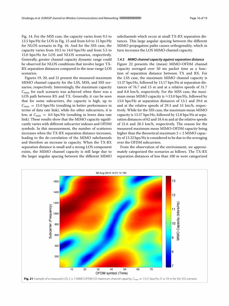
MIMO channel capacity for the LSS, MSS, and SSS sce-narios, respectively. Interestingly, the maximum capacityCmax for each scenario was achieved when there was aLOS path between RX and TX. Generally, it can be seenthat for some subcarriers, the capacity is high, up toCmax = 15.0 bps/Hz (resulting in better performance interms of data rate link), while for other subcarriers, it islow, at Cmin = 4.0 bps/Hz (resulting in lower data ratelink). These results show that the MIMO capacity signifi-cantly varies with different subcarrier indexes and OFDMsymbols. In this measurement, the number of scatterersincreases when the TX-RX separation distance increases,leading to the de-correlation of the MIMO subchannelsand therefore an increase in capacity. When the TX-RXseparation distance is small and a strong LOS componentexists, the MIMO channel capacity is still large due tothe larger angular spacing between the different MIMO

subchannels which occur at small TX-RX separation dis-tances. This large angular spacing between the differentMIMO propagation paths causes orthogonality, which inturn increases the LOS MIMO channel capacity.

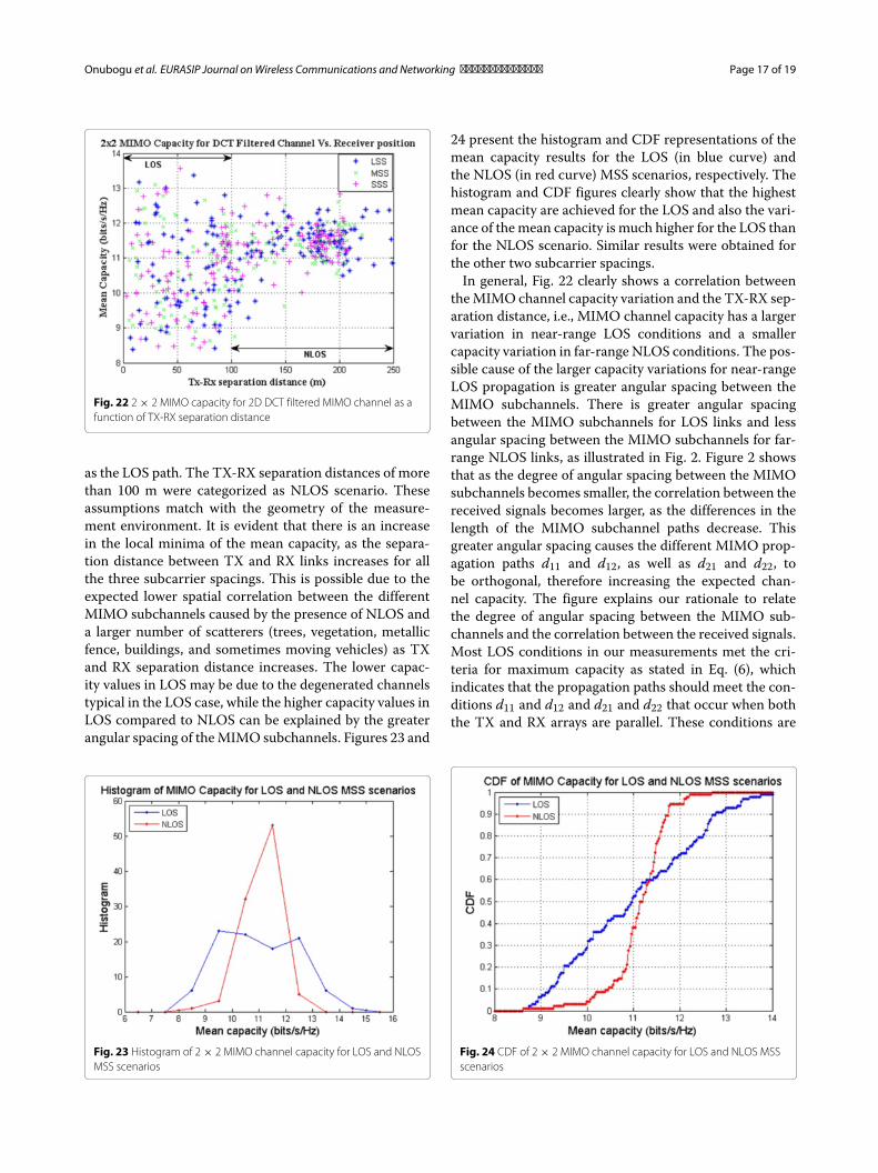
1.4.5 MIMO channel capacity against separation distanceFigure 22 presents the (mean) MIMO-OFDM channelcapacity averaged over 50 ms packet time as a func-tion of separation distance between TX and RX. Forthe LSS case, the maximum MIMO channel capacity is13.37 bps/Hz, followed by 13.17 bps/Hz at separation dis-tances of 76.7 and 15 m and at a relative speeds of 31.7and 8.8 km/h, respectively. For the MSS case, the maxi-mum mean MIMO capacity is ≈13.0 bps/Hz, followed by13.0 bps/Hz at separation distances of 13.1 and 29.6 mand at the relative speeds of 29.3 and 15 km/h, respec-tively. While for the SSS case, the maximummean MIMOcapacity is 13.57 bps/Hz, followed by 12.8 bps/Hz at sepa-ration distances of 62 and 18.4 m and at the relative speedsof 21.6 and 28.3 km/h, respectively. The reason for themeasured maximum mean MIMO-OFDM capacity beinghigher than the theoretical maximum 2×2 MIMO capac-ity of 13.32 bps/Hz is considered to be due to the averagingover the OFDM subcarriers.From the observation of the environment, we approxi-

mately categorized the scenarios as follows. The TX-RXseparation distances of less than 100 m were categorized

Fig. 21 Example of a measured LOS 2 × 2 MIMO-OFDM V2I maximum channel capacity, Cmax = 13.57 bps/Hz, D = 59 m for the SSS scenario


Fig. 22 2 × 2 MIMO capacity for 2D DCT filtered MIMO channel as afunction of TX-RX separation distance

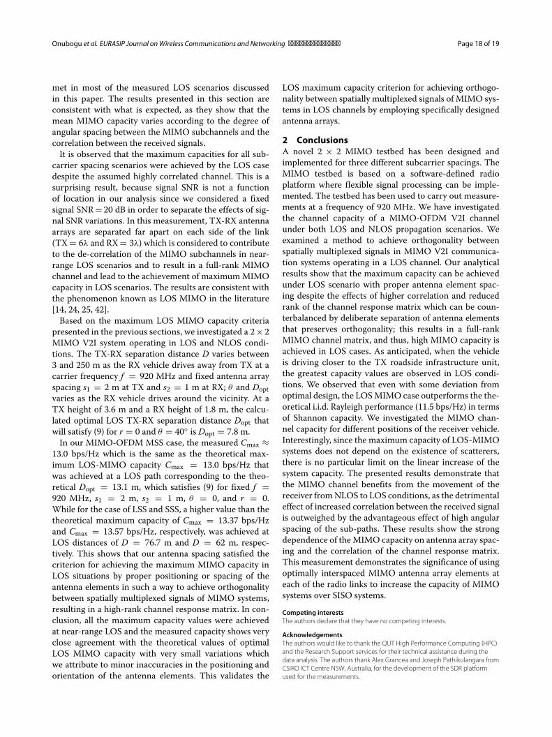
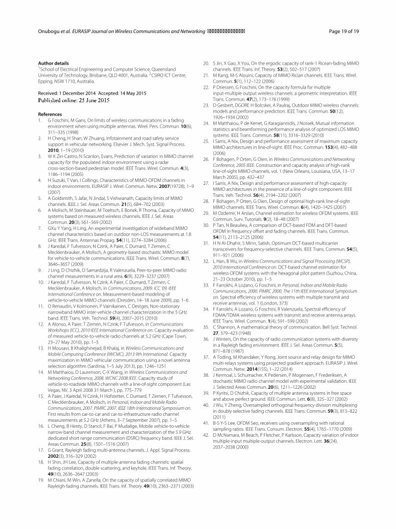
as the LOS path. The TX-RX separation distances of morethan 100 m were categorized as NLOS scenario. Theseassumptions match with the geometry of the measure-ment environment. It is evident that there is an increasein the local minima of the mean capacity, as the separa-tion distance between TX and RX links increases for allthe three subcarrier spacings. This is possible due to theexpected lower spatial correlation between the differentMIMO subchannels caused by the presence of NLOS anda larger number of scatterers (trees, vegetation, metallicfence, buildings, and sometimes moving vehicles) as TXand RX separation distance increases. The lower capac-ity values in LOS may be due to the degenerated channelstypical in the LOS case, while the higher capacity values inLOS compared to NLOS can be explained by the greaterangular spacing of theMIMO subchannels. Figures 23 and

Fig. 23 Histogram of 2 × 2 MIMO channel capacity for LOS and NLOSMSS scenarios

24 present the histogram and CDF representations of themean capacity results for the LOS (in blue curve) andthe NLOS (in red curve) MSS scenarios, respectively. Thehistogram and CDF figures clearly show that the highestmean capacity are achieved for the LOS and also the vari-ance of themean capacity is much higher for the LOS thanfor the NLOS scenario. Similar results were obtained forthe other two subcarrier spacings.In general, Fig. 22 clearly shows a correlation between

theMIMO channel capacity variation and the TX-RX sep-aration distance, i.e., MIMO channel capacity has a largervariation in near-range LOS conditions and a smallercapacity variation in far-range NLOS conditions. The pos-sible cause of the larger capacity variations for near-rangeLOS propagation is greater angular spacing between theMIMO subchannels. There is greater angular spacingbetween the MIMO subchannels for LOS links and lessangular spacing between the MIMO subchannels for far-range NLOS links, as illustrated in Fig. 2. Figure 2 showsthat as the degree of angular spacing between the MIMOsubchannels becomes smaller, the correlation between thereceived signals becomes larger, as the differences in thelength of the MIMO subchannel paths decrease. Thisgreater angular spacing causes the different MIMO prop-agation paths d11 and d12, as well as d21 and d22, tobe orthogonal, therefore increasing the expected chan-nel capacity. The figure explains our rationale to relatethe degree of angular spacing between the MIMO sub-channels and the correlation between the received signals.Most LOS conditions in our measurements met the cri-teria for maximum capacity as stated in Eq. (6), whichindicates that the propagation paths should meet the con-ditions d11 and d12 and d21 and d22 that occur when boththe TX and RX arrays are parallel. These conditions are

Fig. 24 CDF of 2 × 2 MIMO channel capacity for LOS and NLOS MSSscenarios


met in most of the measured LOS scenarios discussedin this paper. The results presented in this section areconsistent with what is expected, as they show that themean MIMO capacity varies according to the degree ofangular spacing between the MIMO subchannels and thecorrelation between the received signals.It is observed that the maximum capacities for all sub-

carrier spacing scenarios were achieved by the LOS casedespite the assumed highly correlated channel. This is asurprising result, because signal SNR is not a functionof location in our analysis since we considered a fixedsignal SNR= 20 dB in order to separate the effects of sig-nal SNR variations. In this measurement, TX-RX antennaarrays are separated far apart on each side of the link(TX= 6λ and RX= 3λ) which is considered to contributeto the de-correlation of the MIMO subchannels in near-range LOS scenarios and to result in a full-rank MIMOchannel and lead to the achievement of maximumMIMOcapacity in LOS scenarios. The results are consistent withthe phenomenon known as LOS MIMO in the literature[14, 24, 25, 42].Based on the maximum LOS MIMO capacity criteria

presented in the previous sections, we investigated a 2× 2MIMO V2I system operating in LOS and NLOS condi-tions. The TX-RX separation distance D varies between3 and 250 m as the RX vehicle drives away from TX at acarrier frequency f = 920 MHz and fixed antenna arrayspacing s1 = 2 m at TX and s2 = 1 m at RX; θ and Doptvaries as the RX vehicle drives around the vicinity. At aTX height of 3.6 m and a RX height of 1.8 m, the calcu-lated optimal LOS TX-RX separation distance Dopt thatwill satisfy (9) for r = 0 and θ = 40◦ is Dopt = 7.8 m.In our MIMO-OFDM MSS case, the measured Cmax ≈

13.0 bps/Hz which is the same as the theoretical max-imum LOS-MIMO capacity Cmax = 13.0 bps/Hz thatwas achieved at a LOS path corresponding to the theo-retical Dopt = 13.1 m, which satisfies (9) for fixed f =920 MHz, s1 = 2 m, s2 = 1 m, θ = 0, and r = 0.While for the case of LSS and SSS, a higher value than thetheoretical maximum capacity of Cmax = 13.37 bps/Hzand Cmax = 13.57 bps/Hz, respectively, was achieved atLOS distances of D = 76.7 m and D = 62 m, respec-tively. This shows that our antenna spacing satisfied thecriterion for achieving the maximum MIMO capacity inLOS situations by proper positioning or spacing of theantenna elements in such a way to achieve orthogonalitybetween spatially multiplexed signals of MIMO systems,resulting in a high-rank channel response matrix. In con-clusion, all the maximum capacity values were achievedat near-range LOS and the measured capacity shows veryclose agreement with the theoretical values of optimalLOS MIMO capacity with very small variations whichwe attribute to minor inaccuracies in the positioning andorientation of the antenna elements. This validates the

LOS maximum capacity criterion for achieving orthogo-nality between spatially multiplexed signals of MIMO sys-tems in LOS channels by employing specifically designedantenna arrays.

2 ConclusionsA novel 2 × 2 MIMO testbed has been designed andimplemented for three different subcarrier spacings. TheMIMO testbed is based on a software-defined radioplatform where flexible signal processing can be imple-mented. The testbed has been used to carry out measure-ments at a frequency of 920 MHz. We have investigatedthe channel capacity of a MIMO-OFDM V2I channelunder both LOS and NLOS propagation scenarios. Weexamined a method to achieve orthogonality betweenspatially multiplexed signals in MIMO V2I communica-tion systems operating in a LOS channel. Our analyticalresults show that the maximum capacity can be achievedunder LOS scenario with proper antenna element spac-ing despite the effects of higher correlation and reducedrank of the channel response matrix which can be coun-terbalanced by deliberate separation of antenna elementsthat preserves orthogonality; this results in a full-rankMIMO channel matrix, and thus, high MIMO capacity isachieved in LOS cases. As anticipated, when the vehicleis driving closer to the TX roadside infrastructure unit,the greatest capacity values are observed in LOS condi-tions. We observed that even with some deviation fromoptimal design, the LOSMIMO case outperforms the the-oretical i.i.d. Rayleigh performance (11.5 bps/Hz) in termsof Shannon capacity. We investigated the MIMO chan-nel capacity for different positions of the receiver vehicle.Interestingly, since the maximum capacity of LOS-MIMOsystems does not depend on the existence of scatterers,there is no particular limit on the linear increase of thesystem capacity. The presented results demonstrate thatthe MIMO channel benefits from the movement of thereceiver fromNLOS to LOS conditions, as the detrimentaleffect of increased correlation between the received signalis outweighed by the advantageous effect of high angularspacing of the sub-paths. These results show the strongdependence of theMIMO capacity on antenna array spac-ing and the correlation of the channel response matrix.This measurement demonstrates the significance of usingoptimally interspaced MIMO antenna array elements ateach of the radio links to increase the capacity of MIMOsystems over SISO systems.

Competing interestsThe authors declare that they have no competing interests.

AcknowledgementsThe authors would like to thank the QUT High Performance Computing (HPC)and the Research Support services for their technical assistance during thedata analysis. The authors thank Alex Grancea and Joseph Pathikulangara fromCSIRO ICT Centre NSW, Australia, for the development of the SDR platformused for the measurements.


Author details1School of Electrical Engineering and Computer Science, QueenslandUniversity of Technology, Brisbane, QLD 4001, Australia. 2CSIRO ICT Centre,Epping, NSW 1710, Australia.

Received: 1 December 2014 Accepted: 14 May 2015

References1. G Foschini, M Gans, On limits of wireless communications in a fading

environment when using multiple antennas. Wirel. Pers. Commun. 10(6),311–335 (1998)

2. H Cheng, H Shan, W Zhuang, Infotainment and road safety servicesupport in vehicular networking. Elsevier J. Mech. Syst. Signal Process.2010, 1–19 (2010)

3. W K Ziri-Castro, N Scanlon, Evans, Prediction of variation in MIMO channelcapacity for the populated indoor environment using a radarcross-section-based pedestrian model. IEEE Trans. Wirel. Commun. 4(3),1186–1194 (2005)

4. H Suzuki, T Van, I Collings, Characteristics of MIMO-OFDM channels inindoor environments. EURASIP J. Wirel. Commun. Netw. 2007(19728), 1–9(2007)

5. A Goldsmith, S Jafar, N Jindal, S Vishwanath, Capacity limits of MIMOchannels. IEEE J. Sel. Areas Commun. 21(5), 684–702 (2003)

6. A Molisch, M Steinbauer, M Toeltsch, E Bonek, R Thoma, Capacity of MIMOsystems based on measured wireless channels. IEEE J. Sel. AreasCommun. 20(3), 561–569 (2002)

7. GXu Y Yang, H Ling, An experimental investigation of wideband MIMOchannel characteristics based on outdoor non-LOS measurements at 1.8GHz. IEEE Trans. Antennas Propag. 54(11), 3274–3284 (2006)

8. J Karedal, F Tufvesson, N Czink, A Paier, C Dumard, T Zemen, CMecklenbrauker, A Molisch, A geometry-based stochastic MIMO modelfor vehicle-to-vehicle communications. IEEE Trans. Wirel. Commun. 8(7),3646–3657 (2009)

9. J Ling, D Chizhik, D Samardzija, R Valenzuela, Peer-to-peer MIMO radiochannel measurements in a rural area. 6(9), 3229–3237 (2007)

10. J Karedal, F Tufvesson, N Czink, A Paier, C Dumard, T Zemen, CMecklenbrauker, A Molisch, in Communications, 2009. ICC ‘09. IEEEInternational Conference on. Measurement-based modeling ofvehicle-to-vehicle MIMO channels (Dresden, 14–18 June 2009), pp. 1–6

11. O Renaudin, V Kolmonen, P Vainikainen, C Oestges, Non-stationarynarrowband MIMO inter-vehicle channel characterization in the 5 GHzband. IEEE Trans. Veh. Technol. 59(4), 2007–2015 (2010)

12. A Alonso, A Paier, T Zemen, N Czink, F Tufvesson, in CommunicationsWorkshops (ICC), 2010 IEEE International Conference on. Capacity evaluationof measured vehicle-to-vehicle radio channels at 5.2 GHz (Cape Town,23–27 May 2010), pp. 1–5

13. H Mousavi, B Khalighinejad, B Khalaj, inWireless Communications andMobile Computing Conference (IWCMC), 2013 9th International. Capacitymaximization in MIMO vehicular communication using a novel antennaselection algorithm (Sardinia, 1–5 July 2013), pp. 1246–1251

14. M Matthaiou, D Laurenson, C-X Wang, inWireless Communications andNetworking Conference, 2008. WCNC 2008 IEEE. Capacity study ofvehicle-to-roadside MIMO channels with a line-of-sight component (LasVegas, NV, 3 April 2008 31 March ), pp. 775–779

15. A Paier, J Karedal, N Czink, H Hofstetter, C Dumard, T Zemen, F Tufvesson,C Mecklenbrauker, A Molisch, in Personal, Indoor andMobile RadioCommunications, 2007. PIMRC 2007. IEEE 18th International Symposium on.First results from car-to-car and car-to-infrastructure radio channelmeasurements at 5.2 GHz (Athens, 3–7 September 2007), pp. 1–5

16. L Cheng, B Henty, D Stancil, F Bai, P Mudalige, Mobile vehicle-to-vehiclenarrow-band channel measurement and characterization of the 5.9 GHzdedicated short range communication (DSRC) frequency band. IEEE J. Sel.Areas Commun. 25(8), 1501–1516 (2007)

17. G Grant, Rayleigh fading multi-antenna channels. J. Appl. Signal Process.2002(3), 316–329 (2002)

18. H Shin, JH Lee, Capacity of multiple-antenna fading channels: spatialfading correlation, double scattering, and keyhole. IEEE Trans. Inf. Theory.49(10), 2636–2647 (2003)

19. M Chiani, M Win, A Zanella, On the capacity of spatially correlated MIMORayleigh-fading channels. IEEE Trans. Inf. Theory. 49(10), 2363–2371 (2003)

20. S Jin, X Gao, X You, On the ergodic capacity of rank-1 Ricean-fading MIMOchannels. IEEE Trans. Inf. Theory. 53(2), 502–517 (2007)

21. M Kang, M-S Alouini, Capacity of MIMO Rician channels. IEEE Trans. Wirel.Commun. 5(1), 112–122 (2006)

22. P Driessen, G Foschini, On the capacity formula for multipleinput-multiple output wireless channels: a geometric interpretation. IEEETrans. Commun. 47(2), 173–176 (1999)

23. D Gesbert, DGORE H Bolcskei, A Paulraj, Outdoor MIMO wireless channels:models and performance prediction. IEEE Trans. Commun. 50(12),1926–1934 (2002)

24. M Matthaiou, P de Kerret, G Karagiannidis, J Nossek, Mutual informationstatistics and beamforming performance analysis of optimized LOS MIMOsystems. IEEE Trans. Commun. 58(11), 3316–3329 (2010)

25. I Sarris, A Nix, Design and performance assessment of maximum capacityMIMO architectures in line-of-sight. IEEE Proc. Commun. 153(4), 482–488(2006)

26. F Bohagen, P Orten, G Oien, inWireless Communications and NetworkingConference, 2005 IEEE. Construction and capacity analysis of high-rankline-of-sight MIMO channels, vol. 1 (New Orleans, Louisiana, USA, 13–17March 2005), pp. 432–437

27. I Sarris, A Nix, Design and performance assessment of high-capacityMIMO architectures in the presence of a line-of-sight component. IEEETrans. Veh. Technol. 56(4), 2194–2202 (2007)

28. F Bohagen, P Orten, G Oien, Design of optimal high-rank line-of-sightMIMO channels. IEEE Trans. Wirel. Commun. 6(4), 1420–1425 (2007)

29. M Ozdemir, H Arslan, Channel estimation for wireless OFDM systems. IEEECommun. Surv. Tutorials. 9(2), 18–48 (2007)

30. P Tan, N Beaulieu, A comparison of DCT-based FDM and DFT-basedOFDM in frequency offset and fading channels. IEEE Trans. Commun.54(11), 2113–2125 (2006)

31. H N Al-Dhahir, S Minn, Satish, Optimum DCT-based multicarriertransceivers for frequency-selective channels. IEEE Trans. Commun. 54(5),911–921 (2006)

32. L Han, B Wu, inWireless Communications and Signal Processing (WCSP),2010 International Conference on. DCT-based channel estimation forwireless OFDM systems with the hexagonal pilot pattern (Suzhou, China,21–23 October 2010), pp. 1–5

33. F Farrokhi, A Lozano, G Foschini, in Personal, Indoor andMobile RadioCommunications, 2000. PIMRC 2000. The 11th IEEE International Symposiumon. Spectral efficiency of wireless systems with multiple transmit andreceive antennas, vol. 1 (London, 373)

34. F Farrokhi, A Lozano, G Foschini, R Valenzuela, Spectral efficiency ofFDMA/TDMA wireless systems with transmit and receive antenna arrays.IEEE Trans. Wirel. Commun. 1(4), 591–599 (2002)

35. C Shannon, A mathematical theory of communication. Bell Syst. Technol.27, 379–423 (1948)

36. J Winters, On the capacity of radio communication systems with diversityin a Rayleigh fading environment. IEEE J. Sel. Areas Commun. 5(5),871–878 (1987)

37. A Toding, M Khandaker, Y Rong, Joint source and relay design for MIMOmulti-relays systems using projected gradient approach. EURASIP J. Wirel.Commun. Netw. 2014(155), 1–22 (2014)

38. J Kermoal, L Schumacher, K Pedersen, P Mogensen, F Frederiksen, Astochastic MIMO radio channel model with experimental validation. IEEEJ. Selected Areas Commun. 20(6), 1211–1226 (2002)

39. P Kyritsi, D Chizhik, Capacity of multiple antenna systems in free spaceand above perfect ground. IEEE Commun. Lett. 6(8), 325–327 (2002)

40. J Wu, Y Zheng, Oversampled orthogonal frequency division multiplexingin doubly selective fading channels. IEEE Trans. Commun. 59(3), 815–822(2011)

41. B-S Y-S Lee, OFDM Seo, receivers using oversampling with rationalsampling ratios. IEEE Trans. Consum. Electron. 55(4), 1765–1770 (2009)

42. D McNamara, M Beach, P Fletcher, P Karlsson, Capacity variation of indoormultiple-input multiple-output channels. Electron. Lett. 36(24),2037–2038 (2000)

Documents

RESEARCH OpenAccess Experimentalevaluationofthe ... · RESEARCH OpenAccess Experimentalevaluationofthe ... of an experimental investigation of 2 × 2 MIMO-OFDM channel measurements