i " NASA-CR-'I-96608

1 _LIGHT-

/ •

!.

i .

[ .

RESEARCH

LABORATORY

G

÷

$

YOF

o_

O, ¢I N

U C_

Z _ 0

THE UNIVERSITY OF KANSAS CENTER FOR RESEARCH, INC.

2201 Irving HIll Drive

Lawrence, Kansas 66045-2060

0

https://ntrs.nasa.gov/search.jsp?R=19940014975 2018-08-26T10:43:43+00:00Z

AN INVESTIGATION OF

FIGHTER AIRCRAFT AGILITY

KU-FRL-831-7

5 November 1993

FINAL TECHNICAL REPORT

NCC 2-588 Phases I-V, 01/01/89 - 12/31/93

John Valasek

and

David R. Downing, Principal Investigator

THE UNIVERSITY OF KANSAS CENTER FOR RESEARCH, INC.

Flight Research Laboratory

2291 Irving Hill Drive

Lawrence, Kansas 66045

(913) 864-3043

prepared for

Joseph Gera and Robert Clarke, Technical MonitorsNASA Ames Research Center

Dryden Flight Research Facility

ABSTRACT

This report attempts to unify in a single document the results of a series of studies on fighter

aircraft agility funded by the NASA Ames Research Center, Dryden Flight Research Facility and

conducted at the University of Kansas Hight Research Laboratory during the period January 1989

through December 1993. New metrics proposed by pilots and the research community to assess

fighter aircraft agility are collected and analyzed. The report develops a framework for understanding

the context into which the various proposed fighter agility metrics fit in terms of application and

testing. Since new metrics continue to be proposed, this report does not claim to contain every

proposed fighter agility melric. Hight test procedures, test constraints, and related criteria are

developed. Instrumentation required to quantify agility via flight test is considered, as is the

sensitivity of the candidate metrics to deviations from nominal pilot command inputs, which is studied

in detail. Instead of supplying specific, detailed conclusions about the relevance or utility of one

candidate metric versus another, the authors have attempted to provide sufficient data and analyses

for readers to formulate their own conclusions. Readers are therefore ultimately responsible for

judging exactly which metrics are "best" for their particular needs. Additionally, it is not the intent

of the authors to suggest combat tactics or other actual operational uses of the results and data in this

report. This has been left up to the user community.

Twenty of the candidate agility metrics were selected for evaluation with high fidelity,

nonlinear, non real-time flight simulation computer programs of the F-5A Freedom Fighter, F-16A

Fighting Falcon, F-18A Hornet, and X-29A. The information and data presented on the 20 candidate

metrics which were evaluated will assist interested readers in conducting their own extensive

investigations. The report provides i) a definition and analysis of each metric; ii) details of how to

test and measure the metric, including any special data reduction requirements; iii) typical values for

the metric obtained using one or more aircraft types, and iv) a sensitivity analysis ff applicable.

The report is organized as follows. The first chapter in the report presents a historical review

of air combat trends which demonstrate the need for agility metrics in assessing the combat

performance of fighter aircraft in a modern, all-aspect missile environment. The second chapter

presents a framework for classifying each candidate metric according to time scale (transient,

functional, instantaneous), further subdivided by axis (pitch, lateral, axial). The report is then broadly

divided into two parts, with the transient agility metrics (pitch lateral, axial) covered in chapters three,

four, and five, and the functional agility metrics covered in chapter six. Conclusions,

recommendations, and an extensive reference list and biography are also included. Five appendices

contain a comprehensive list of the definitions of all the candidate metrics collected by the

investigators; a description of the aircraft models and flight simulation programs used for testing the

metrics; several relations and concepts which are fundamental to the study of lateral agility; an in-

depth analysis of the axial agility metrics; and a derivation of the relations for the instantaneous agility

metrics and thek approximations, including an example of their use.

ii

PREFACE

This report is a summary of fighter agility metrics research conducted by the University of

Kansas Flight Research Laboratory from the period January 1989 through December 1993. This work

was conducted by several researchers, and resulted in five reports, six theses, five conference papers,

and two journal articles. The objective of this report was to collect the individual reports and theses

and supplement them with new material in order to present a comprehensive and coherent overview.

In addition to the authors, the researchers who have contributed to this report are Randall K. Liefer,

David P. Eggold, Brian W. Cox, George W. Ryan HI, and Frank H. Liu.

In the course of this study, the researchers have received assistance and many valuable

suggestions. The authors extend their appreciation and thanks to the following persons: Joseph Gera,

Robert Clarke, and Joseph Wilson of the NASA Ames Research Center, Dryden Flight Research

Facility; Edward D. Onstott of the Northrop Corporation, Aircraft Division; Herbert H. Hickey Jr., G.

Thomas Black, and William T. Thomas of the Air Force Wright Research and Development Center;

Major Bob Vosburgh and Major Dale A. Nagy, United States Air Force; Major Steven Grohsmeyer,

United States Marine Corps.

°°°

Ill

TABLE OF CONTENTS

ABSTRACT .......................................................... i

PREFACE ........................................................... iii

TABLE OF CONTENTS ................................................. iv

LIST OF FIGURES ..................................................... xiv

°°°

LIST OF TABLES .................................................... xxm

NOMENCLATURE .................................................... xxiv

° INTRODUCTION

1.1

1.2

1.3

° o ° , , , , , ° ° ° , ° ° ° , ° ° ° ° ° , ° ° ° ° o ° ° ° ° ° , ° ° ° ° ° ° , ° • * * * ° ° * 1

BACKGROUND OF AGILITY METRICS RESEARCH ................ 1

REPORT OBJECTIVE ....................................... 5

REPORT ORGANIZATION ................................... 6

, CLASSIFICATION OF AGILITY METRICS ............................. 7

2° 1 BACKGROUND ............................................ 7

2°2 CLASSIFICATION FRAMEWORK .............................. 7

2.2.1

2.2.2

2.2.3

Transient, Functional, Potential ............................ 7

Lateral, Pitch, Axial .................................... 9

Agility Classification Matrix .............................. 9

iv

. PITCH AGILITY ................................................

3.1 BACKGROUND ...........................................

3.2 CANDIDATE PITCH AGILITY METRICS ........................

3,3 PITCH AGILITY TESTING AND

DATA REDUCTION TECHNIQUES ............................

3.4 CANDIDATE PITCH AGILITY METRICS RESULTS ................

3.4.2

3.4.3

3.4.4

11

11

11

12

17

Maximum Positive Pitch Rate ............................ 17

3.4.1.1 Definition ............................... 17

3.4.1.2 Discussion And Typical Results ............... 17

3.4.1.3 Maximum Positive Pitch Rate Sensitivity ......... 20

3.4.1.4 Summary ............................... 22

Maximum Negative Pitch Rate ........................... 22

3.4.2.1 Definition ............................... 22

3.4.2.2 Discussion And Typical Results ............... 23

3.4.2.3 Maximum Negative Pitch Rate Sensitivity ........ 25

3.4.2.4 Summary ............................... 26

Maximum Positive And Negative Pitch Rate From

An Initial Angle Of Attack .............................. 27

3.4.3.1 Definition ............................... 27

3.4.3.2 Discussion And Typical Results ............... 27

3.4.3.3 Summary ............................... 29

Time To Pitch To Maximum Normal Load Factor .............. 30

3.4.4.1 Definition ............................... 30

3.4.4.2 Discussion And Typical Results ............... 30

3.4.4.3 Time To Pitch To Maximum Normal

Load Factor Sensitivity ..................... 33

V

3.5

3.4.5

3.4.6

3.4.7

3.4.4.4 Summary ................................ 34

Time to Pitch Down From Maximum

Normal Load Factor to 0g ............................... 35

3.4.5.1 Definition ............................... 35

3.4.5.2 Discussion And Typical Results ............... 35

3.4.5.3 Time To Pitch Down From Maximum

Normal Load Factor To 0g Sensitivity ........... 37

3.4.5.4 Summary ............................... 38

Positive Normal Load Factor Rate ...................... .... 39

3.4.6.1 Definition ............................... 39

3.4.6.2 Discussion And Typical Results ............... 39

3.4.6.3 Positive Normal Load Factor Rate Sensitivity ...... 42

3.4.6.4 Summary ............................... 42

Negative Normal Load Factor Rate ........................ 43

3.4.7.1 Definition ............................... 43

3.4.7.2 Discussion And Typical Results ............... 43

3.4.7.3 Negative Normal Load Factor Rate Sensitivity ..... 44

3.4.7.4 Summary ............................... 46

3.4.8 Avergage Pitch Rate .................................... 46

3.4.8.1 Definition ............................... 46

3.4.8.2 Discussion And Typical Results ............... 46

3.4.8.3 Average Pitch Rate Sensitivity ................ 50

3.4.8.4 Summary ............................... 51

SUMMARY .............................................. 52

vi

. LATERAL AGILITY

4.1

4.2

4.3

4.4

4.5

. o...........o o..........................o... 54

BACKGROUND ........................................... 54

CANDIDATE LATERAL AGILITY METRICS ..................... 54

LATERAL AGILITY TESTING AND

DATA REDUCTION TECHNIQUES ............................ 55

4.3.1 Measurement Criteria For Time Through 90 ° Roll Angle Metric .... 58

4.3.2 Capture Criteria For The 90 ° Roll Angle Capture Metric ......... 58

4.3.3 180 ° Roll Angle Capture Metric ........................... 63

CANDIDATE LATERAL AGILITY METRICS RESULTS ............. 67

4.4.1 Time Through 90 ° Roll Angle ('l'ax90) 67

4.4.1.1 Definition ............................... 67

4.4.1.2 Discussion And Typical Results ............... 67

4.4.1.3 Average Pitch Rate Sensitivity ................ 71

4.4.1.4 Summary ............................... 72

4.4.2 900 Roll Angle Capture (TRcgo) ........................... 73

4.4.2.1 Definition ............................... 73

4.4.2.2 Discussion And Typical Results ............... 73

4.4.2.3 90 ° Roll Angle Capture Sensitivity ............. 75

4.4.2.4 Summary ............................... 77

4.4.3 180 ° Roll Angle Capture (Ttc_so) .......................... 78

4.4.3.1 Definition ............................... 78

4.4.3.2 Discussion And Typical Results ............... 78

4.4.3.3 180 ° Roll Angle Capture Sensitivity ............. 87

4.4.3.4 Summary ............................... 89

SUMMARY .............................................. 90

vii

. AXIAL AGILITY

5.1

5.2

5.3

5.4

5.5

.........,.°o. oo ........Qo.o.....-*.....'''*''" 92

BACKGROUND ........................................... 92

CANDIDATE AXIAL AGILITY METRICS ....................... 92

AXIAL AGILITY TESTING AND

DATA REDUCTION TECHNIQUES ............................ 93

CANDIDATE AXIAL AGILITY METRICS RESULTS ............... 97

5.4.1 Power Onset Parameter ................................. 97

5.4.1.1 Definition ............................... 97

5.4.1.2 Discussion And Typical Results ............... 97

5.4.1.3 Summary ............................... 100

5.4.2 Power Loss Parameter ................................. 100

5.4.2.1 Definition ............................... 100

5.4.2.2 Discussion And Typical Results ............... 100

5.4.2.3 Summary ............................... 102

SUMMARY .............................................. 102

. FUNCTIONAL AGILITY

6.1

6.2

6.3

6.4

..............oo..**ooo..... 1.. o...-..*... 104

BACKGROUND ........................................... 104

CANDIDATE FUNCTIONAL AGILITY METRICS .................. 105

FUNCTIONAL AGILITY TESTING AND

DATA REDUCTION TECHNIQUES ............................ 105

CANDIDATE FUNCTIONAL AGILITY METRICS RESULTS .......... 112

6.4.1 Combat Cycle Time 180 ° Heading Change ................... 112

6.4.1.1 Definition ............................... 112

6.4.1.2 Discussion And Typical Results ............... 112

VIL1

6.4.2

6.4.3

6.4.4

6.4.5

6.4.6

6.4.1.3 Combat Cycle Time 18&

Heading Change Sensitivity .................. 119

6.4.1.4 Summary ............................... 121

Combat Cycle Time 90° Heading Change .................... 123

6.4.2.1 Definition ............................... 123

6.4.2.2 Discussion And Typical Results ............... 124

6.4.2.3 Combat Cycle Time 90*Heading Change Sensitivity .................. 124

6.4.2.4 Summary ............................... 126

Dynamic Speed Turn .................................. 127

6.4.3.1 Definition ............................... 127

6.4.3.2 Discussion And Typical Results ............... 127

6.4.3.3 Dynamic Speed Turn Sensitivity ............... 135

6.4.3.4 Summary ............................... 138

Relative Energy State (V/V_) ............................. 139

6.4.4.1 Definition ............................... 139

6.4.4.2 Discussion And Typical Results ............... 139

6.4.4.3 Relative Energy State Sensitivity ............... 140

6.4.4.4 Summary ............................... 142

Energy-Agility ....................................... 143

6.4.5.1

6.4.5.2

6.4.5.3

6.4.5.4

_me-Energy _nalty

Definition ............................... 143

Discussion And Typical Results ............... 143

Energy-Agility Sensitivity .................... 146

Summary ............................... 150

.................................. 150

ix

6.5

6.4.6.1

6.4.6.2

6.4.6.3

6.4.6.4

Definition ............................... 150

Discussion And Typical Results ............... 150

Time-Energy Penalty Sensitivity ............... 153

Summary ............................... 154

155

°

°

°

CONCLUSIONS ................................................ 158

RECOMMENDATIONS ........................................... 161

REFERENCES .................................................. 163

APPENDIX A:

A.1

A.2

A.3

CANDIDATE AGILITY METRICS ............................ A1

BACKGROUND ........................................... A1

CANDIDATE PITCH AGILITY METRICS ........................ A1

A.2.1 Time Derivative of Load Factor ........................... A1

A.2.2 Time To Capture A Specified Angle Of Attack ................ A2

A.2.3 Time To Change Pitch Attitude ........................... A2

A.2.4 Maximum Nose-Up And Nose-Down Pitch Rate ............... A3

A.2.5 Pitch Agility ........................................ A3

A.2.6 Average Pitch Rate ................................... A4

A.2.7 Pitch Agility Criteria .................................. A5

CANDIDATE LATERAL AGILITY METRICS ..................... A6

A.3.1 Lateral Agility TRcgo ................................... A6

A.3.2 Lateral Agility TRcls0 .................................. A7

A.3.3

A.3.4

A.3.5

A.3.6

A.3.7

A.3.g

Roll Angle Capture ................................... A7

Time Through Roll Angle ................................ A7

Roll Reversal Capture .................................. A8

Defensive Roll Reversal Agility Parameter ................... A9

Torsional Agility, TR/TRcso .......................... .... A10

Roll Transient ....................................... A11

A.4 . CANDIDATE AXIAL AGILITY METRICS ....................... A12

A.4.1 Axial Agility ........................................ A12

A.5 CANDIDATE FUNCTIONAL AGILITY METRICS .................. A13

A.5.1 Combat Cycle Time ................................... A13

A.5.2 Dynamic Speed Turn .................................. A14

A.5.3 Relative Energy State .................................. A14

A.5.4 Energy-Agility ....................................... A15

A.5.5 Time-Energy Penalty .................................. A16

A.5.6 DT Parameter ........................ : .............. A17

A.5.7 Pointing Margin ...................................... A18

A.5.8 One-Circle Pointing Quotient ............................ A19

A.6 CANDIDATE AGILITY POTENTIAL METRICS ................... A20

A.6.1 Agility Potential and Maneuvering Potential .................. A20

A.7 CANDIDATE INSTANTANEOUS AGILITY METRICS .............. A21

A.7.1 Curvature Agility ..................................... A21

A.7.2 Herbst Torsional Agility ................................ A22

xi

APPENDIXB:

B.1

B.2

B.3

e°4

B.5

B.6

FLIGHT SIMULATION PROGRAMS ...........................

BACKGROUND ...........................................

GENERIC Fo5A SIX DEGREE-OF-FREEDOM

AIRCRAFT SIMULATION (ATHP) .............................

GENERIC F-16A SIX DEGREE-OF-FREEDOM

AIRCRAFT SIMULATION (F-16SIM) ...........................

GENERIC F-18A SIX DEGREE-OF-FREEDOM

AIRCRAFT SIMULATION (SIM-IO ............................

GENERIC X-29A SIX DEGREE-OF-FREEDOM

AIRCRAFT SIMULATION ................................ ....

OPTIMAL TRAJECTORIES BY IMPLICIT

SIMULATION PROGRAM (OTIS) .............................

B1

B1

B1

B2

B4

B6

B9

APPENDIX C:

C.1

C.2

C.3

C.4

C.5

ADDITIONAL LATERAL AGILITY CONSIDERATIONS ............ C1

BACKGROUND ........................................... C1

AXIS SYSTEMS .......................................... C1

ROLLING ABOUT THE VELOCITY VECTOR .................... C2

COUPLING EFFECTS ...................................... C10

PILOT CONSIDERATIONS .................................. C12

APPENDIX D:

D.1

D.2

ADDmONAL AXIAL AGILITY CONSIDERATIONS .............. D1

BACKGROUND ........................................... D1

THE COMPONEN'I_ OF AXIAL AGILITY ........................ D1

APPENDIX E:

E.1

E.2

DERIVATION OF INSTANTANEOUS AGILITY METRICS .......... E1

BACKGROUND ........................................... E1

CANDIDATE INSTANTANEOUS AGILITY METRICS .............. E1

xii

E.3

E.4

E.5

E.2.1 Curvature Agility ..................................... E1

E.2.2 Herbst Torsional Agility ................................ E2

DERIVATION AND APPROXIMATION TO

THE INSTANTANEOUS AGILITY METRICS ..................... E2

INSTANTANEOUS AGILITY RESULTS ......................... E6

E.4.1 Curvature Agility Results ............................... E6

E.4.2 Herbst Torsional Agility Results .......................... E7

SUMMARY .............................................. E7

,°,

xln

LIST OF FIGURES

21.1 Historical Trends In Air Combat ......................................

92.1 Proposed Classification Framework ....................................

3.1 Typical Pilot Stick Input Commands And Data ExtractionPoints Used For Evaluating Pitch Agility Metrics .......................... 14

3.2 Generic F-5A, F-16A, and F-18A Maximum Positive Pitch

Rate From Steady Level Flight, H = 500 feet ............................ 18

3.3 Generic F-5A, F-16A, andF-18A Maximum Positive Pitch

Rate From Steady Level Flight, H = 15,000 feet .......................... 19

3.4 Generic F-5A, F-16A, and F-18A Maximum Positive Pitch

Rate From Steady Level Flight, H = 40,000 feet .......................... 20

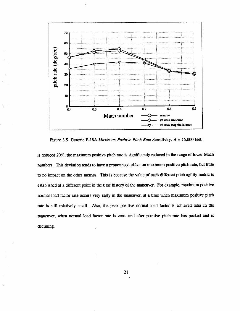
3.5 Generic F-18A Maximum Positive Pitch Rate

Sensitivity, H = 15,000 feet ......................................... 21

3.6 Generic F-5A, F-16A, and F-18A Maximum NegativePitch Rate, H = 500 feet ........................................... 23

3.7 Generic F-5A, F-16A, and F-18A Maximum Negative

Pitch Rate, H - 15,000 feet ......................................... 24

3.8 Generic F-5A, F-16A, and F-18A Maximum NegativePitch Rate, H = 40,000 feet ......................................... 25

3.9 Generic F-18A Maximum Negative Pitch Rate

Sensitivity, H = 15,000 feet ......................................... 26

3.10 Generic F-18A Maximum Positive Pitch Rate From An

Initial Angle Of Attack, H = 15,000 feet ................................ 28

xiv

3.11 Generic F-18A Maximum Negative Pitch Rate From An

Initial Angle Of Attack, H = 15,000 feet ................................ 29

3.12 Generic Fo5A, F-16A, And F-18A Time To Pitch Up ToMaximum Normal Load Factor, H = 500 feet ............................ 31

3.13 Generic F-5A, F-16A, And F-18A Time To Pitch Up ToMaximum Normal Load Factor, H = 15,000 feet .......................... 32

3.14 Generic F-5A, F-16A, And F-18A Time To Pitch Up ToMaximum Normal Load Factor, H = 40,000 feet .......................... 33

3.15 Generic F-18A Time To Pitch Up To Maximum

Normal Load Factor Sensitivity, H = 15,000 feet .......................... 34

3.16 Generic F-5A, F-16A, And F-18A Time To Pitch Down From

Maximum Normal Load Factor To 0g, H -- 500 feet ....................... 35

3.17 Generic F-5A, F-16A, And F-18A Time To Pitch Down From

Maximum Normal Load Factor To 0g, H = 15,000 feet ..................... 36

3.18 Generic F-5A, F-16A, And F-18A Time To Pitch Down From

Maximum Normal Load Factor To 0g, H = 40,000 feet ..................... 37

3.19 Generic F-18A Time To Pitch Down From Maximum

Normal Load Factor To 0g Sensitivity, H = 15,000 feet ..................... 38

3.20 Generic F-5A, F-16A, And F-18A Positive Normal

Load Factor Rate, H = 500 feet ................... . .................. 40

3.21 Generic F-SA, F-16A, And F-18A Positive Normal

Load Factor Rate, H = 15,000 feet .................................... 41

3.22 Generic F-5A, F-16A, And F-18A Positive Normal

Load Factor Rate, H = 40,000 feet .................................... 41

XV

3.23 Generic F-18A Positive Normal Load Factor

Rate Sensitivity, H = 15,000 feet ..................................... 42

3.24 Generic F-5A, F-16A, And F-18A Negative NormalLoad Factor Rate, H - 500 feet ...................................... 43

3.25 Genetic F-5A, F-16A, And F-18A Negative NormalLoad Factor Rate, H -- 15,000 feet .................................... 44

3.26 Generic F-5A, F-16A, And F-18A Negative Normal

Load Factor Rate, H = 40,000 feet .................................... 45

3.27 Genetic F-18A Negative Normal Load Factor

Rate Sensitivity, H -- 15,000 feet ..................................... 45

3.28 Generic F-5A, F-16A, And F-18A Pitch Rate From Level

Flight Time History, Mach - 0.7, H -- 15000 feet ......................... 47

3.29 Generic F-5A, F-16A, And F-18A Average Pitch

Rate From Level Hight, H - 500 feet .................................. 48

3.30 Genetic F-5A, F-16A, And F-18A Average Pitch

Rate From Level Hight, H = 15,000 feet ................................ 49

3.31 Generic F-5A, F-16A, And F-18A Average Pitch

Rate From Level Flight, H -- 40,000 feet ................................ 50

3.32 Genetic F-18A Average Pitch Rate From Level

Flight Sensitivity, H -- 15,000 feet .................................... 51

4.1 Typical Lateral Stick Time History Used To Roll

Through A Target Bank Angle ....................................... 57

4.2 Typical Lateral Stick Time History Used To

Capture A Target Bank Angle ....................................... 58

xvi

4.3 TypicalPilot Stick Input Commands And Data Extraction Points

Used For Testing The Time Through 900 Roll Angle Metric .................. 59

4.4 Typical Pilot Stick Input Commnads And Data Extraction PointsUsed For Testing The 90 ° Roll Angle Capture Metric ....................... 61

4.5 Effest ,Of Normalization On The Time To Roll And Capture 90 °,Generic F-18A, Mach = 0.4, H = 15,000 feet ............................ 62

4.6 Generic F-18A Unsatisfactory Target Bank Angle Capture For

The 90 ° Roll Angle Capture Metric, H -- 15,000 feet ....................... 62

4.7 Typical Pilot Stick Input Commands And Data Extraction PointsUsed For Testing The 1800 Roll Angle Capture Metric ...................... 64

4.8 Application Of The Bank Angle Capture Criteria ForTesting The 180 ° Roll Angle Capture Metric ............................. 65

4.9 Generic F-5A Time Through 90° Roll AngleMetric Results, H = 15,000 feet ...................................... 68

4.10 Generic F-16A Time Through 900 Roll AngleMetric Results, H = 15,000 feet ...................................... 69

4.11 Generic F-18A Time Through 90° Roll AngleMetric Results, H = 15,000 feet ...................................... 70

4.12 Generic F-18A Average Normal Load Factor During A Time

Through 90 ° Roll Angle Maneuver, H - 15,000 feet ........................ 71

4.13

4.14

Generic F-18A Maximum Sideslip Angle During A Time

Through 900 Roll Angle Maneuver, H = 15,000 feet ........................

Generic F-5A 90 ° Roll Angle Capture MetricResults, H = 15,000 feet .............................................

72

73

xvii

4.15 GenericF-16A900Roll Angle Capture MetricResults, H = 15,000 feet ........................................... 74

4.16 Generic F-18A 90 ° Roll Angle Capture MetricResults, H = 15,000 feet ........................................... 75

4.17 Generic F-18A 900 Roll Angle CaptureSensitivity, H -- 15,000 feet ......................................... 76

4.18 Genetic F-5A And Generic F-18A 1800 Roll Angle

Capture Metric Results, H = 15,000 feet ................................ 79

4.19 Generic F-5A And Generic F-18A Average Normal Load Factor

During A 180 ° Roll Angle Capture Maneuver, H -- 15,000 feet ................ 79

4.20 Comparison Of Generic F-5A And Generic F-18A Parameters DuringA 180 ° Roll Angle Capture, Average Angle Of Attack 7°, 0.7/15k .............. 81

4.21 Generic F-18A 180 ° Roll Angle Capture Trajectory,

Average Angle Of Attack 7°, 0.7/15k .................................. 82

4.22 Generic F-18A Parameters During A 180 ° Roll Angle

Capture, Average Angle Of Attack 16°, 0.7/15k ........................... 83

4.23 Generic F-18A Control Surface Activity During A 180 ° Roll

Angle Capture, Average Angle Of Attack 16°, 0.7/15k ...................... 85

4.24 Generic F-18A 180 ° Roll Angle Capture

Sensitivity, Mach -- 0.7, H = 15,000 feet ................................ 88

5.1 Command Time Histories For Testing The Power Onset Parameter ............. 94

5.2

5.3

Command Time Histories For Testing The Power Loss Parameter .............. 96

Power Onset Parameter For The Generic F-16A and Generic F-18A ............ 98

XVlll

5.4 Effect of Transition Times on The Power Onset Parameter ................... 99

5.5 Power Loss Parameter For The Generic F-16A and Generic F-18A ............. 101

6.1 Maneuver Segments Of A Typical Combat Cycle Time Plot .................. 107

6.2 Typical Pilot Stick And Throttle Input CommandsUsed For Testing The Combat Cycle Time Metric ......................... 108

6.3 Angle Of Attack Time History Match For The OTISand Generic F-18A Simulations ................................... ... 111

6.4 Generic F-5A 180 ° Combat Cycle Time Plot ............................. 113

6.5 Generic F-16A 180 ° Combat Cycle Time Plot ............................ 114

6.6 Generic F-18A 180 ° Combat Cycle Time Plot ............................ 115

6.7 Generic F-18A Drag Build-Up And Speed Loss

During 180 ° Heading Change ........................................ 116

6.8 Generic X-29A 180 ° Combat Cycle Time Plot ............................. 117

6.9 Maneuver Segment Times Of The Generic F-5A, F-16A, F-18A,

and X-29A During A 180 ° Combat Cycle Time Maneuver Sequence ............ 118

6.10 Generic F-18A 1800 Combat Cycle Time Sensitivity,Mach -- 0.8, H = 15,000 feet ........................................ 120

6.11 Generic F-18A 180 ° Combat Cycle Time Sensitivity Angle

Of Attack Comparison, Mach= 0.8, H - 15,000 feet ....................... 121

6.12 Generic F-5A 90 ° Combat Cycle Time Plot, Maeh -- 0.8, H - 15,000 feet ........ 125

xix

6.13 Generic F-16A 90 ° Combat Cycle Time Plot, Mach = 0.8, H - 15,000 feet ........ 125

6.14 Generic F-18A 90 o Combat Cycle Time Plot, Mach= 0.8, H = 15,000 feet ........ 126

6.15 Generic F-5A Dynamic Speed Turn Plots, Maeh = 0.8, H = 15,000 feet .......... 128

6.16 Generic F-16A Dynamic Speed Turn Plots, Math = 0.8, H = 15,000 feet ......... 130

6.17 Generic F-18A Dynamic Speed Turn Plots, Maeh = 0.8, H = 15,000 feet ......... 131

6.18 Generic X-29A Dynamic Speed Turn Plots, Mach = 0.8, H = 15,000 feet ......... 133

6.19 Comparison Of Generic F-5A, F-16A, F-18A, and X-29ADynamic Speed Turn Plots, Mach = 0.8, H - 15,000 feet .................... 134

6.20 Genetic Fol8A Dynamic Speed Turn Sensitivity, Mach= 0.8, H = 15,000 feet ..... 136

6.21 Generic F-5A, F-16A, F-18A, And X-29A Relative Energy State

For Various Heading Angles, Mach= 0.8, H = 15,000 feet ................... 140

6.22 Comparison Of Generic F-SA, F-16A, F-18A, And X-29A Angle Of AttackTime Histories For A 180 _ Turn, Math = 0.8, H = 15,000 feet ................ 141

6.23 Generic F-18A Relative Energy State Sensitivity,Mach = 0.8, H = 15,000 feet ......................................... 142

6.24 Generic F-5A Energy-Agility Plot, Maeh = 0.8, H = 15,000 feet ............... 144

6.25 Generic F-16A Energy-Agility Plot, Magh = 0.8, H = 15,000 feet .............. 145

6.26 Genetic F-18A Energy-Agility Plot, Math = 0.8, H = 15,000 feet .............. 145

6.27 Generic X-29A Energy-Agility Plot, Mach= 0.8, H = 15,000 feet .............. 146

XX

6.28

6.29

Comparison Of Generic F-5A, F-16A, F-18A, And X-29A

Overshoot Of Heading Angle Required To Capture 180 °,Mach -- 0.8, H = 15,000 feet ........................................

Generic F-18A Energy-Agility Sensitivity, Mach = 0.8, H - 15,000 feet ..........

147

148

6.30 Comparison Of Generic F-18A Heading Angle Overshoots From

Energy-Agility Sensitivity, Math = 0.8, H = 15,000 feet ..................... 149

6.31 Generic F-5A, F-16A, F-18A, And X-29A 180 ° Time-Energy

Penalty Plot, Math - 0.8, H = 15,000 feet .............................. 151

6.32 Generic F-5A, F-16A, F-18A, And X-29A 90 ° Time-Energy

Penalty Plot, Math -- 0.8, H = 15,000 feet .............................. 152

6.33 Generic F-18A 180 ° Time-Energy Penalty Sensitivity,

Mach = 0.8, H = 15,000 feet ........................................ 153

6.34 Generic F-18A 90 ° Time-Energy Penalty Sensitivity,

Mach -- 0.8, H = 15,000 feet ........................................ 155

B.1 F-5A External Physical Characteristics ................................. B3

B.2 F-16A External Physical Characteristics ................................ B5

B.3 F- 18A External Physical Characteristics ................................ B7

B.4 X-29A External Physical Characteristics ................................ B8

C.1 Geometric Relationships Between Body Axes,

Stability Axes, And Wind Axes ...................................... C1

C.2 Required Combinations Of Body Axis Roll And Yaw RatesFor Stability Axis Roll Rates ........................................ C5

xxi

C.3 Generic F-18A Response To Full Lateral Stick Command,Aft Stick = 1.5 inches, Mach = 0.4, H = 15,000 feet ....................... C7

C.4 Components Of Sideslip Rate Resulting From A Full Lateral

Stick Command, Generic F-18A, Aft Stick = 1.5 inches,

Mach= 0.4, H = 15,000 feet ........................................ C8

C.5 Source Of Kinematic Coupling Into Sideslip Resulting From A FullLateral Stick Command, Generic F-18A, Aft Stick = 1.5 inches,

Mach= 0.4, H - 15,000 feet ........................................ C8

C.6 Components Of Angle Of Attack Rate Resulting From A Full LateralStick Command, Generic F-18A, Aft Stick = 1.5 inches,

Mach= 0.4, H = 15,000 feet ........................................ el0

C.7 Pitching Momem Due To Inertial Coupling .............................. C12

C.8 Components Of Lateral Acceleration At The Pilot Station

During A Full Lateral Stick Command, Generic F-18A,Aft Stick = 1.5 inches, Mach= 0.4, H = 15,000 feet C14

D.1 Terms In Approximation of APs/At, Power Onset Parameter,Generic F-18A, Mach = 0.7, H = 15,000 feet ............................ D3

E.1 Geometry of the Maneuver Plane in a Steady Level Turn .................... E3

E.2 Definition of Serret-Frenet Roll Angle _ and Roll Rate P=.. pbm_ ............... EA

E.3 Comparison Of Approximation To The Curvature Agility Metric,

-15 ° To 10 ° Pitch Capture, 200 KTAS, Angle Of Attack = 15° ................ E7

E.4 Comparison Of Approximation To The Herbst Torsional Agility

Metric, 5g Roll Maneuver, Mach= 0.7, H = 15,000 feet ..................... E8

xxii

LIST OF TABLES

3.1 Deviations For Pitch Sensitivity Testing ................................ 16

4.1 Errors And Magnitudes For Roll Angle Capture Metrics

Sensitivity Analysis .............................................. 67

6.1 180 ° Combat Cycle Times For The Generic F-5A, F-16A,F-18A, and X-29A, Math = 0.8, H = 15,000 feet .......................... 119

6.2 Generic F-18A 180 ° Combat Cycle Time SensitivityResults, Math = 0.8, H = 15,000 feet .................................. 122

C.1 Lateral Acceleration at Pilot Station Requirement ......................... C14

C.2 Effect of High Lateral Accelerations on Pilot

Physiology and Mission Effectiveness ................................. C16

XXlll

NOMENCLATURE

ADI

AIM

AOA

alpha

ATHP

b

beta

BVR

CLmax

Cm_

Cm 8

CCT

CG

D

DEG

DT

EM

FCS

FS

GLOC

attitudedirectionindicator

aircraftinterception missile

angleof attack

centripetalacceleration

angleof attack

aircrafttimehistoryprogram

wing span

sideslipangle

beyond visualrange

maximum liftcoefficient

variationof pitchingmoment coefficientdue toangleof attack

variationof pitchingmoment coefficientdue topitchconlzoleffectors

combat cycletime metric

centerof gravity

mean aerodynamic chord

drag

degrees

product of crossrange and lime metric

energy maneuverability

flight conU'ol system

fuselage station •

g induced loss of consciousness

xxiv

degrees

fee_/sec 2

degrees

feet

degrees

seconds

feet

pounds

feet-seconds

inches

g

H

HARV

HUD

h,

IR

Ixz

Ixx, Izz

KIAS

KTAS

KU/FRL

k

L

L

LEX

lbf

M

M

MC-C

MvN

gravitational acceleration

altitude

high angle of attack research vehicle

head up display

specific energy height

infrared

XZ product of inertia

moment of inertia about X, Y, Z axes

indicated airspeed

true airspeed

University of Kansas Flight Research Laboratory

xlO 3

lift

rolling moment

leading edge extcmion

pounds force

pitching moment

Mach number

pitching moment due to inertial coupling

starting or initial Math number

test Mach number

mean geometric chord

some quantity "M" versus some quantity "N"

feet/see 2

feet

feet

slug-feed

.slug-feed

knots

knOts

pounds

foot-pounds

foot-pounds

foot-pounds

XXV

M8

N

NASA

N,

n

n(+),n(-)

nx

ny

nz

OTIS

P

Pm_n plane

Ps

P

Q

q

R

REF

r

S

SEC

dimensional variation of pitching moment

due to pitch control effectors

yawing moment

national aeronautics and space administration

normal load factor

normal load factor

upper and lower boundaries of n in the service flight envelope

axial load factor

lateral load factor

normal load factor

optimal trajectories by implicit simula_on

body axis roll rate

maneuver plane roll rate

specificexcesspower

stabilityaxisrollrate

perturbedbody axisrollrate

body axispitchrate

perturbedbody axispitchrate

dynamic pressure

body axisyaw rate

reference

perturbed body axis yaw rate

wing area

seconds

seconds-2

foot-pounds

g's

g's

g's

g's

g'S

degress/second

degrees/second

feet/second

degrees/second

degrees/second

degrees/second

degrees/second

pounds/feed

degrees/second

degrees]second

feed

xxvi

SLS

T

TEl'

TO

TR

Tm_ s

Ttcoo

TRc,so

T_o

%0

t

tk

V

VIFFING

V_

v,

W

WVR

X

Y

Y

Z

sea level static

thrust

time-energy penalty metric

take off

turn rate

time to achieve maximum normal load factor metric

time to roll and capture a bank angle near 90 °

time to roll and capture a 900 bank angle change metric

time to roll and capture a 1800 bank angle change metric

time to roll through a 90° bank angle metric

time to pitch from maximum normal load factor to Og melric

time to roll through a 90 ° bank angle change metric

time

time to kill

total velocity

vectoring in forward flight

corner

true speed

weight

within visual range

aircraft longitudinal axis

aircraft lateral axis

crossrange

aircraft transverse axis

pounds

feet-seconds

degrees/second

seconds

seconds

seconds

seconds

seconds

seconds

seconds

seconds

seconds

feet/second

feet/second,knots

feet/second,knots

pounds

feet

xxvii

et

A

e,e

o,¢

X

(0

lvl

angle of attack

sideslip angle

pitch angle or flight path angle in Serret-Frenet reference plane

incremental value

pitchattitudeangle

rollsubsidencemode time constant

bank angle

headingangleinSerret-Frenetreferenceplane

headingangle

turn rate

roll angle in Serret-Frenet reference plane

one-verus-one

degrees

degrees

degrees

degrees

seconds

degrees

degrees

degree,s

degrees/second

degrees

SUBSCRHrFS

B, body body fixed axes

max maximum value

rain minimum value

n normal component

S, stab stabilityaxes

W, wind relativewind axes

x axialcomponent

SUPERSCRIPTS

derivative with respect to time

o*.

XXVlU

1. INTRODUCTION

1.1 BACKGROUND OF AGILITY METRIC RESEARCH

Fighter flying qualifies and combat capabilities are currently measured and compared in terms

relating to vehicle energy, angular rates and sustained acceleration. Criteria based on these measurable

quantifies have evolved over the past several decades and are routinely used to design aircraft

structures, aer .odynamics, propulsion and control systems. While these criteria, or metrics, have the

advantage of being well understood, easily verified and repeatable during test, they tend to measure

the steady state capability of the aircraft and not its ability to transition quickly from one state to

another (REF. 1, 2, 3).

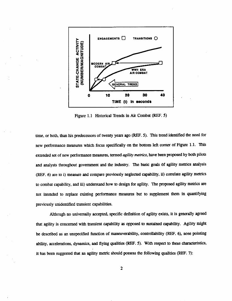
Figure 1.1 displays historical trends in the close or within-visual-range (WVR) air combat

arena. In the past, the necessity of achieving stable, rear quarter firing solutions led to extended

engagement times and steady state maneuvering. Traditional measures of merit such as maximum

level speed, turn rate, rate of climb, and maximum normal load factor were found to be adequate for

quantifying aircraft capabilities. Recently, the introduction of lethal, reliable, all-aspect, short range

missiles such as the AIM-9L Sidewinder have diminished the emphasis on sustained maneuvering

capability. Engagement times have been decreased by nearly an order of magnitude as pilots need

only to point their weapons at the target in order to achieve a high probability of kill.

The emphasis now is to "point and shoot" first (REF. 4).

Point and shoot requires an instantaneous maneuver capability (translational and rotational

accelerations) and nonsymmetric or uncoordinated dynamic maneuvers (sideslip _ 0, sideforce _ 0).

As a result the capability to change aircraft states as quickly as possible has become an important

factor for success in modern air combat. This means the modern fighter pilot is required to execute

the same number of state changes faster, or change a greater number of states in the same length of

<_,

ENGAGEMENTS[] TRANSITIONSC)

Figure 1.1

MODERN

ERAAIR COMBAT

ENERAL TRENDI

0 10 20 30 40

TIME (t) In ucond$

Historical Trends in Air Combat (REF. 5)

time, or both, than his predecessors of twenty years ago (REF. 5). This trend identified the need for

new performance measures which focus specifically on the bottom left comer of Figure 1.1. This

extended set of new performance measures, termed agility metrics, have been proposed by both pilots

and analysts throughout government and the industry. The basic goals 0f agility metrics analysis

(REF. 6) are to i) measure and compare previously neglected capability, ii) correlate agility metrics

to combat capability, and iii) understand how to design for agility. The proposed agility metrics are

not intended to replace existing performance measures but to supplement them in quantifying

previously unidentified transient capabilities.

Although no universally accepted, specific definition of agility exists, it is generally agreed

that agility is concerned with transient capability as opposed to sustained capability. Agility might

be described as an unspecified function of maneuverability, controllability (REF. 6), nose pointing

ability, accelerations, dynamics, and flying qualities (REF. 5). With respect to these characteristics,

it has been suggested that an agility metric should possess the following qualities fREF. 7):

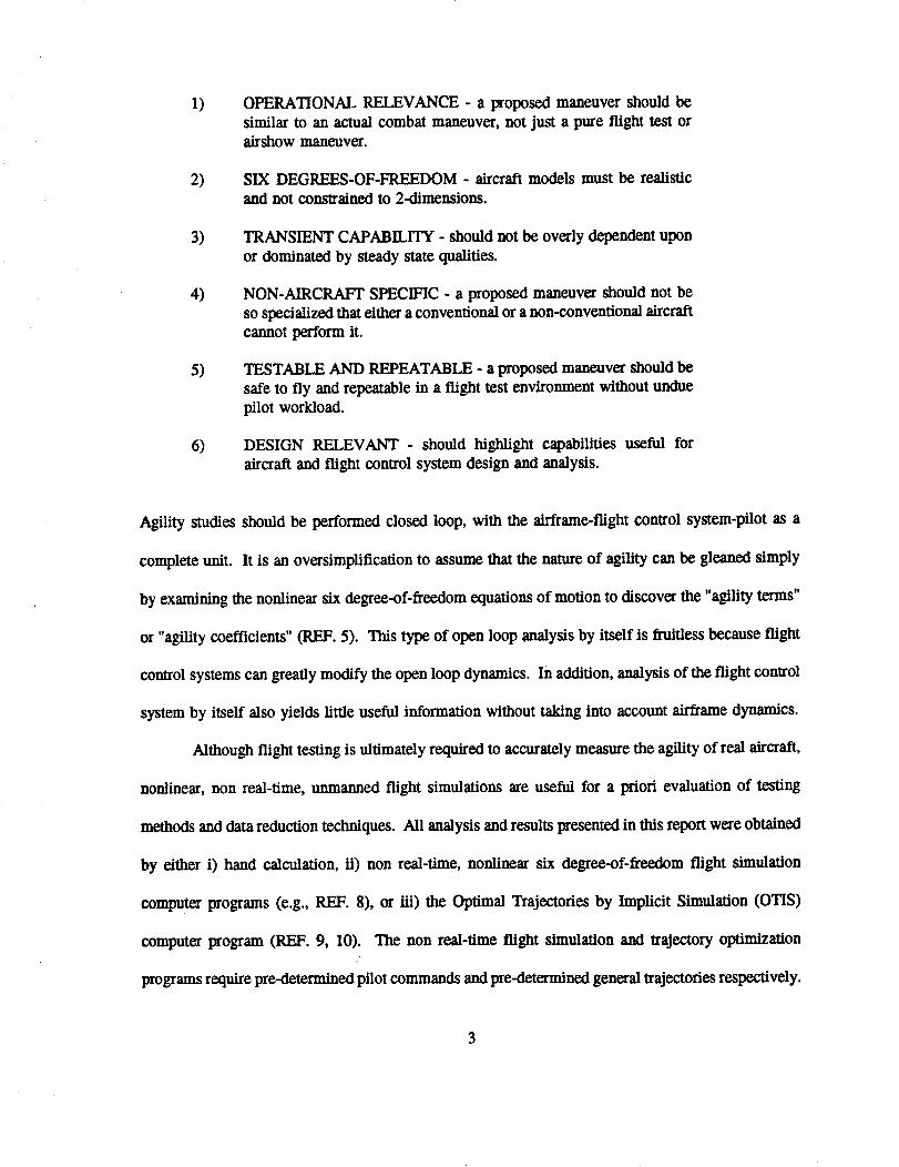
1)

2)

3)

4)

5)

6)

OPERATIONAL RELEVANCE - a proposed maneuver should be

similar to an actual combat maneuver, not just a pure flight test orail"show maneuver,

SIX DEGREES-OF-FREEDOM - aircraft models must be realistic

and not constrained to 2-dimensions.

TRANSIENT CAPABILITY - should not be overly dependent upon

or dominated by steady state qualities.

NON-AIRCRAFT SPECIFIC - a proposed maneuver should not be

so specialized that either a conventional or a non-conventional aircraft

cannot perform it.

TESTABLE AND REPEATABLE - a proposed maneuver should be

safe to fly and repeatable in a flight test environment without undue

pilot workload.

DESIGN RELEVANT - should highlight capabilities useful for

aircraft and flight control system design and analysis.

Agility studies should be performed closed loop, with the airframe-flight control system-pilot as a

complete unit. It is an oversimplification to assume that the nature of agility can be gleaned simply

by examining the nonlinear six degree-of-freedom equations of motion to discover the "agility terms"

or "agility coefficients" (REF. 5). This type of open loop analysis by itself is fruitless because flight

control systems can greatly modify the open loop dynamics. In addition, analysis of the flight control

system by itself also yields little useful information without taking into account airframe dynamics.

Although flight testing is ultimately required to accurately measure the agility of real aircraft,

nonlinear, non real-time, unmanned flight simulations are useful for a priori evaluation of testing

methods and data reduction techniques. All analysis and results presented in this report were obtained

by either i) hand calculation, ii) non real-time, nonlinear six degree-of-freedom flight simulation

computer programs (e.g., REF. 8), or iii) the Optimal Trajectories by Implicit Simulation (OTIS)

computer program (REF. 9, 10). The non real-time flight simulation and trajectory optimization

programs require pre-determined pilot commands and pre-determined general trajectories respectively.

This necessitates analysis of deviations from the nominal pilot command inputs, so where applicable

these sensitivities are included in this report.

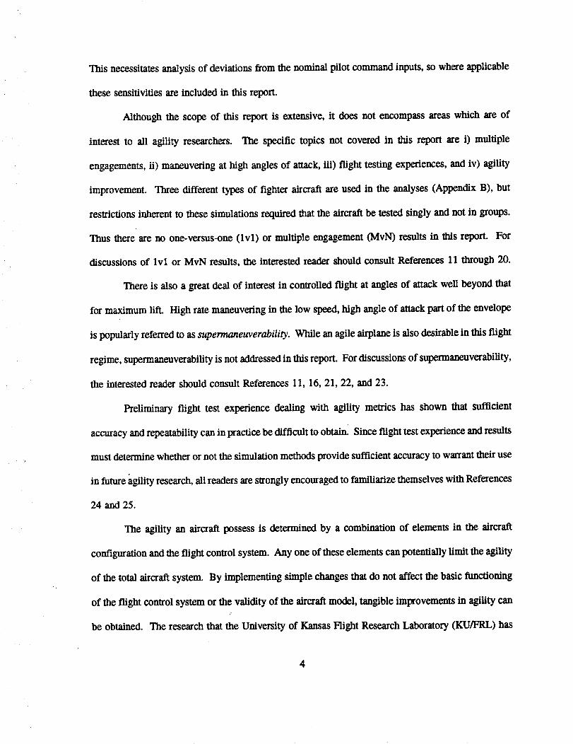
Although the scope of this report is extensive, it does not encompass areas which are of

interest to all agility researchers. The specific topics not covered in this report are i) multiple

engagements, ii) maneuvering at high angles of attack, ili) flight testing experiences, and iv) agility

improvement. Three different types of fighter aircraft are used in the analyses (Appendix B), but

restrictions inherent to these simulations required that the aircraft be tested singly and not in groups.

Thus there are no one-versus-one (lvl) or multiple engagement (MvN) results in this report. For

discussions of lvl or MvN results, the interested reader should consult References 11 through 20.

There is also a great deal of interest in controlled flight at angles of attack well beyond that

for maximum lift. High rate maneuvering in the low speed, high angle of attack part of the envelope

is popularly referred to as supermaneuverabiliry. While an agile airplane is also desirable in this flight

regime, supermaneuverability is not addressed in this report. For discussions of supermaneuverability,

the interested reader should consult References 11, 16, 21, 22, and 23.

Preliminary flight test experience dealing with agility metrics has shown that sufficient

accuracy and repeatability can in practice be difficult to obtain. Since flight test experience and results

must determine whether or not the simulation methods provide sufficient accuracy to warrant their use

in future agility research, all readers are strongly encouraged to familiarize themselves with References

24 and 25.

The agility an aircraft possess is determined by a combination of elements in the aircraft

configuration and the flight control system. Any one of these elements can potentially limit the agility

of the total aircraft system. By implementing simple changes that do not affect the basic functioning

of the flight control system or the validity of the aircraft model, tangible improvements in agility can

be obtained. The research that the University of Kansas Hight Research Laboratory (KU/FRL) has

4

conducted in improving the agility of an existing aircraft is not contained in this report, but is

presented in References 26, 27, and 28.

1.2 REPORT OBJECTIVE

This report attempts to compile in a single document the results of a series of studies

supported by the NASA Ames Dryden Flight Research Facility and conducted at the KU/FRL during

the period January 1989 through July 1993. The majority of the results presented in this report were

obtained by several KU/FRL investigators, and comments on experiences and results of the

investigations are limited to work performed solely by them. The authors have generated new

unpublished results to compliment and unify the previously published data. The intent of the authors

is not to suggest combat tactics or other actual operational uses of the results and data in this report.

This has been left up to the user community.

The report provides a framework for understanding the context into which the various

proposed fighter agility metrics fit in terms of application and testing. Since new metrics continue

to be proposed, this report does not claim to contain every agility metric. Results for those candidate

metrics which were investigated are usually presented for only a small number of flight conditions,

since this research was intended to identify candidate agility metrics and investigate their

characteristics, rather than perform exhaustive analyses over the entire operational flight envelope.

However, the information and data presented in this report should be sufficient to permit interested

readers to conduct their own extensive investigations. Readers interested in investigating a particular

metric should be able to locale i) a definition of the metric; ii) an explanation of how to test and

measure the metric, including any special data reduction requirements; iii) typical values for the metric

obtained using one or more aircraft types, and iv) a sensitivity analysis if applicable.

5

Instead of supplying specific, detailed conclusions about the relevance or utility of particular

metrics, the authors have attempted to provide sufficient data and analyses for readers to formulate

their own conclusions. Readers are ultimately responsible for judging exactly which metrics are ,'best"

for their particular needs.

1.3 REPORT ORGANIZATION

This report is broadly divided into two parts; the transient agility metrics are covered in

Chapters 2 through 5, and the functional agility metrics are covered in Chapter 6. Chapter 2 presents

a framework for classifying the candidate agility metrics investigated. Chapters 3 through 6 each

examine a particular class of metrics, according to the framework established in Chapter 2. In each

chapter a definition, background discussion, testing methods, and data reduction methods are

presented. Typical results and a discussion of sensitivity to testing errors are also presented where

appropriate. Pitch agility is investigated in Chapter 3, lateral agility in Chapter 4, and axial agility

in Chapter 5. Functional agility is investigated in Chapter 6. Conclusions and recommendations are

presented in Chapters 7 and 8 respectively. A comprehensive list of all of the candidate metrics

investigated in this report is contained in Appendix A. Appendix B contains a description of the

aircraft models and flight simulation programs used for the investigations. Appendix C develops

several relations and concepts which are fundamental to the study of lateral agility. Appendix D

examines the axial agility metrics in depth. Appendix E derives the relations for the instantaneous

agility metrics and their approximations, and demonstrates their use.

6

2. CLASSIFICATION OF AGILITY METRICS

2.1 BACKGROUND

Since the pilots, engineers and researchers now involved in agility have, as yet, not reached

a commonly accepted definition of the term, it is not surprising that the proposed agility metrics deal

with many different aspects of fighter capability. The various metrics proposed to measure agility deal

in units of time, velocity, angular rate, distance and combinations of time, rate and distance. One of

the first tasks undertaken in this research was the establishment of a method to classify the numerous

metrics suggested by researchers from industry and government laboratories. Although not unique,

the following classification framework has been found to be useful.

2.2 CLASSIFICATION FRAMEWORK

After collecting and reviewing the candidate metrics now available in the literature, it is

apparent that they may be divided into two categories or classes. First, the candidate metrics can be

grouped by time scale into classes referred to by some authors as functional and transient (REF. 24,

29). Secondly, the metrics may be classified according to type of motion involved, e.g. translational

(axial), longitudinal, and lateral.

Each of these two schemes of metric classification are discussed below. The resulting

framework is then presented in a matrix format.

2.2.1 Transient, Functiona L Potential

Regardless of the motion variables involved or the units chosen, all of the proposed agility

metrics can be grouped into one of two time scales. Agility in the context of the short time scale, on

the order of one to three seconds_ is frequently called transient agility (REF. 4, 18, 29). The transient

7

agility metrics are a means to quantify a fighters ability to generate controlled angular motion and to

transition quickly between minimum and maximum levels of specific excess power.

A second group of time dependent metrics called large amplitude metrics (REF. 29) or

functional agility metrics (REF. 24) deals with a longer time scale of ten to twenty seconds. This

class seeks to quantify how well the fighter executes rapid changes in heading or rotations of the

velocity vector. The emphasis is on energy lost during turns through large heading angles and the

time required to recover kinetic energy after unloading to zero normal load factor. Many of these

functional metrics involve maneuvers made up of a sequence of brief segments of transient agility

metrics. For example, the combat cycle time metric (REF. 30) consists of a pitch to maximum normal

load factor, a turn at maximum normal load factor to some specified new heading angle, a pitch down

to zero normal load factor and an acceleration to the original airspeed. The net effect of combining

a sequence of maneuvers and flight segments into a single metric is that conventional aircraft

performance, that is, thrust to weight ratio and sustained normal load factor or turn rate capability,

tend to dominate the metric. In addition to measuring the aircraft capability, these functional agility

metrics also depend heavily on complex pilot inputs which are in turn influenced by the pilot's skill,

experience, the aircraft's flying qualities and the effect of cockpit displays and cues.

A third group of metrics has appeared which are independent of time and so are neither

transient or large amplitude in nature. These melrics deal not with the aircraft characteristics

demonstrated via flight test or simulation but with the agility potential that results from sizing and

configuration choices. These agility potential metrics serve to highlight the (sometimes obvious)

relationships between thrust, weights, inertias, control power and agility. While they have the

advantage of using data available early in the aircraft design cycle, they tend not to reflect the impact

of cross axis nonlinearity or flight control system response characteristics (REF. 31).

8

2.2.2 Lateral_ Pitch_ Axial

Agility metrics may also be classified according to the type of aircraft motion being studied

independent of time scale. Lateral agility metrics include those that deal primarily with rolling

motion, especially rolling at high angles of attack. Longitudinal or pitch agility metrics involve only

pitching motion and normal acceleration. Finally, a number of metrics have been proposed to quantify

the ability of the aircraft to transition between energy states or specific excess power (P,) levels.

These are commonly referred to as axial agility metrics and involve only translational motion.

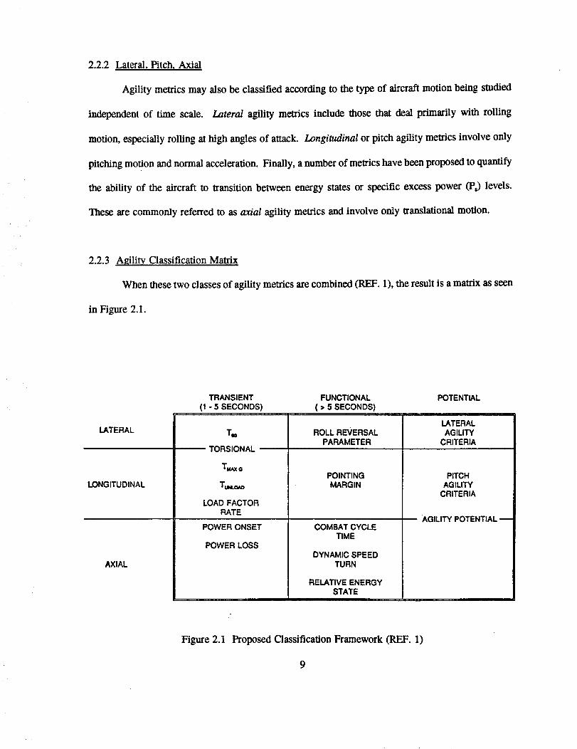
2.2.3 Agility Classification Matrix

When these two classes of agility metrics are combined (REF. 1), the result is a matrix as seen

in Figure 2.1.

TRANSIENT FUNCTIONAL POTENTIAL

(1 - 5 SECONDS) ( > 5 SECONDS)

LATERAL

LONGITUDINAL

AXIAL

T,,,

TORSIONAL

T,_xa

Tu_.o_

LOAD FACTORRATE

POWER ONSET

POWER LOSS

ROLL REVERSALPARAMETER

POINTINGMARGIN

COMBAT CYCLETIME

DYNAMIC SPEEDTURN

RELATIVE ENERGYSTATE

LATERALAGILITY

CRITERIA

PITCHAGILITY

CRITERIA

AGILITY POTENTIAL

Figure 2.1 Proposed Classification Framework (REF. 1)

9

Nearly all of the candidate agility metrics can be placed in a unique position in the matrix. For

instance, pointing margin is a functional agility metric concerned with the longitudinal aircraft axis.

The two exceptions are torsional agility and agility potential. Torsional agility is deliberately

formulated to mix pitching and rolling characteristics and is the ratio of turn rate to the time to roll

and capture a 90 ° bank angle change (REF. 18). The other exception, agility potential, is the ratio of

two traditional performance metrics: wing loading, which is related to longitudinal maneuverability,

and thrust to weight ratio.

Beginning with Chapter 3, each matrix element will be discussed. The order of presentation

is pitch 0ongitudinal) agility in Chapter 3, lateral agility in Chapter 4, axial agility in Chapter 5,

functional agility in Chapter 6, instantaneous agility in Chapter 7, and agility improvement in

Chapter 8.

10

3. PITCH AGILITY

3.1 BACKGROUND

Pitch agility metrics are intended to quantify the motions in the vertical plane or longitudinal

capabilities of fighter aircraft. This class of metrics typically involve only pitching motions and

normal acceleration. This chapter defines the candidate metrics and then details the method of testing

used. The methods used to compare results are also presented. For the results contained in this

chapter, pitch agility is quantified using nonlinear, non real-time, six degree-of-freedom flight

simulation computer programs. Results and analysis are presented for the F-5A, F-16A, and F-18A.

Experiments consist of pre-specified maneuvers designed to quantify the pitch agility of the aircraft.

The acceptability of such maneuvers m an operational pilot, the associated issues of flying qualities,

pilot discomfort, and g-induced loss of consciousness are not addressed in this report.

3.2 CANDIDATE PITCH AGILITY METRICS

Numerous metrics have been proposed to quantify pitch agility including:.

1)

2)

3)

4)

5)

6)

7)

8)

maximum positive and negative pitch rate from steady level flight

maximum positive pitch rate from an initial angle of attack

maximum negative pitch rate from an initial angle of attack

time to pitch to maximum normal load factor

time to pitch down from maximum load factor to zero load normal factor

maximum positive normal load factor rate

maximum negative normal load factor rate

average pitch rate

11

9)

10)

11)

12)

timeto capturea specified angle of attack

time to change pitch attitude

pitch agility criteria

maximum initial pitch acceleration

All of these candidate metrics are investigated with the exception of time to capture a specified angle

of attack, time. to change pitch attitude, pitch agility criteria, and maximum initial pitch acceleration.

These metrics are not investigated in this report because of unsatisfactory results from previous testing,

or because they have been generally rejected by agility researchers (Appendix A).

3.3 PITCH AGILITY TESTING AND DATA REDUCTION TECHNIQUES

The candidate pitch agility metrics listed in Section 3.2 which are tested using non real-time

simulation at altitudes of 500 feet, 15,000 feet and 30,000 feet, and at subsonic Mach numbers ranging

from 0.4 to 0.9. The Mach numbers and altitudes are selected to be representative of those at which

fighter aircraft are most likely to be engaged in within visual range air combat. The metrics

investigated in this report are evaluated in both the nose up and nose down directions.

During subsequent testing of each candidate pitch agility metric (REF. 1, 2, 3), it was

determined that a value for each metric at a given test point could be obtained from a single data

conection run, using a standardized pilot command. This technique simplifies the task for both the

pilot and fight test engineer. The standardized pilot command input consists of an abrupt step input

which is held for two seconds, after which the step command is abruptly taken back out (Figure 3.1).

The duration of the step input is sufficiently long enough for various maximum values and maximum

rates to be achieved. Thus the pilot is not burdened with having to determine whether he has achieved

12

themaximumvalues and rates. This gives the test engineer clearly defined reference points for

measuring the "time to" metrics, using the time at which the pitch-up is initiated, and the time at

which the pitch-down is initiated. Generalizing the command inputs for each candidate pitch agility

metric to a single standardized input sequence is an approximation, but it simplifies the test procedure

and considerably reduces the number of data collection runs.

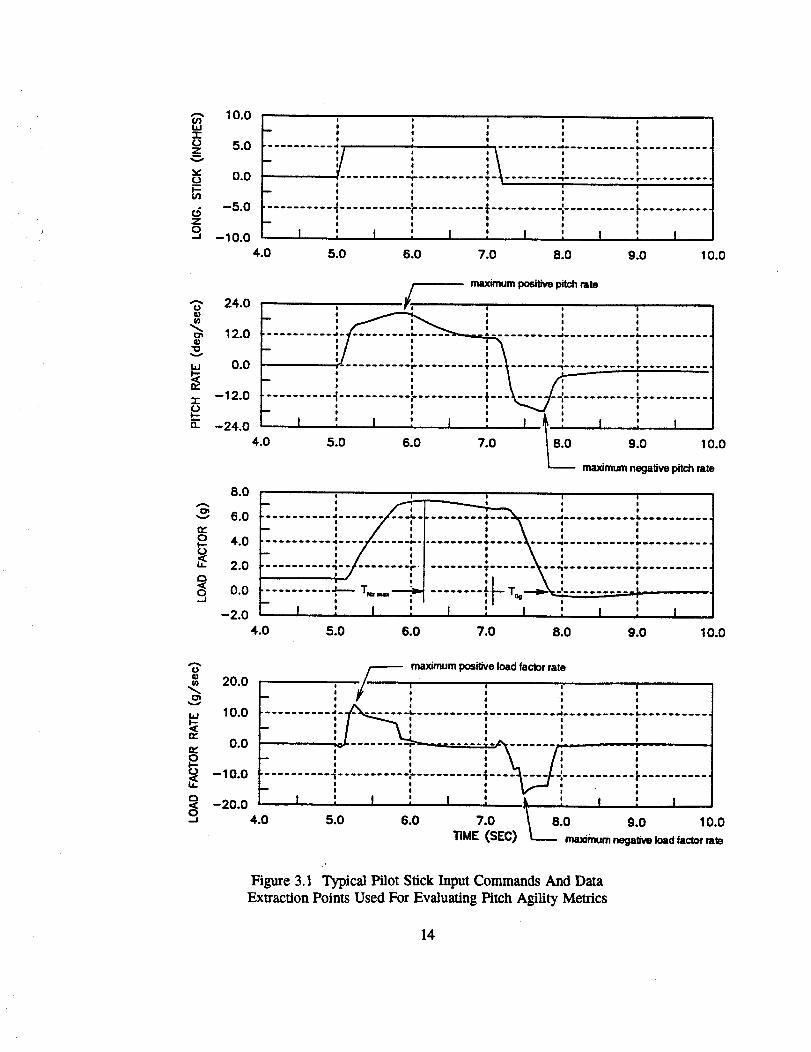
At each flight condition investigated, the aircraft is trimmed to straight and level flight. Step

inputs of maximum aft stick deflection are applied to the longitudinal stick and held for two seconds.

Forward stick was then applied to pitch down to zero normal load factor. Figure 3.1. is a typical

simulation time history from a data collection run, showing how the lime to load, unload and the

associated pitch rates and load factor rates are extracted. Note especially that the time to pitch down

to zero normal load factor is calculated from the time forward stick is commanded, not from the time

that normal load factor begins to decay due to airspeed loss. This method minimizes the influence

of aircraft drag characteristics on pitch agility measurements and emphasizes nose down pitch

authority.

The test technique described above is adequate only for aircraft like the F-16A and F-18A

whose flight control systems incorporate pitch rate and load factor limiters. Applying full aft stick

in aircraft such as the F-5, F-4, or F-15 will at many flight conditions over stress the pilot and aircraft.

In these types of aircraft, the pilot must limit pitch rate and normal load factors manually. As a result,

care must be taken when directly comparing the pitch agility of two aircraft like the F-5 and F- 18A,

whose flight control systems are fundamentally different. One option is to define the maximum

surface deflection permissible for each aircraft at a given flight condition, and then base the agility

measurement on that deflection instead of maximum stick input. This would make flight test much

more difficult since information about surface position is not available to the pilot during flight. Also,

this method would not account for the effects of control surfaces such as maneuvering flaps. These

13

LI.J

C.)z

V

v'o_l-

dZ

B

10.0

5.0

0.0

-5.0

--10.04.0

! I I o$ I I !

I $

•4 I I ----_--o_----d----_. Q.----_..e.. boo...... •

w ! I e !

I ! I I! ! I

o o o--oo------,.,T-, o. oo _.. o. I • ...o...... ...... _...r.._....._.. o

I I e -- ,

I $ I I I

I I $ !

.......... _........... :- .......... .t-.......... -_........... F...........I I l I O

-- t I I I I

! I I I $I , I , I , I , ! , I

5.0 6.0 7.0 8.0 9.0 10.0

_" 24.0O)

g3

o_ 12.0Q)

i 0.0--12.0

0. -24.0

4.0

maximum posilJve pitch rote

I,O O !

| ! I

O l I

I O I

311 : ,r_ l l l

l I l

.--..o.. l.....o.....l .....o. ....

..........+...... .....B

I I I I_ ', _ _ , I

I , I ', i : I : I : I

5.0 6.0 7.0 9.0 10.0

_mt_ n_d_ pkeh rote

8.0

V

Q_0

6.0

4.0

2.0

0.0

-2.04.0

I I

B ! I

-- l I

I !

............+--

I , I t

5.0 6.0

I I l

l I

l I I

I l l

l I It

e i il i l

l l I

I I I

e i l

1 , I , I ,I I I

7.0 8.0 g.o 10.0

¢D

m 20.0

,,, 10.0

iv0.0

-10.0

_ -20.0 4.0

F-- max_um posilJve load factor ratel J I I I I

l JIP I e i e-- e i ii l l

e I e l l

.--o--..o.+--A. ----....._._..._.....................__........... ....

I I I I I

l I l I II l l l l

l I I /-i I

-- I $ I l II

I l e I l

,,+0--+00 .._o l I I I I-- --.oo._.o...r 0_0 ..o_.+.,

e e i e e- : : : , . ,l I l I II , I , I , L . I , I

5.0 6.0 7.0 "I 8.0 9.0 I 0.0TIME (SEC) _ mammumnega_.e load factorm_

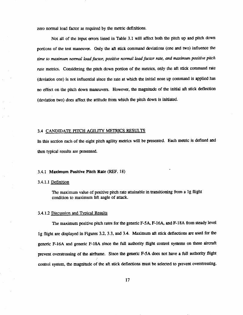
Figure 3.1 Typical Pilot Stick Input Commands And Data

Extraction Points Used For Evaluating Pitch Agility Metrics

14

surfaces are present on the F-18A but are not installed on the generic F-5A.

The time rate of change of normal load factor and average pitch rate are not available either

as a term in the dynamic models of the aircraft or as an output of a modelled sensor. A simple

differencing scheme is used to measure the normal load factor rate. A similar approach would be

needed to obtain this data from a flight test maneuver. In the simulations used with no random

atmospheric inputs, buffeting, or sensor noises, the differencing algorithm produced usable normal load

factor rate data. Applicalion of a differencing scheme to obtain normal load factor rate information

from flight test might require extensive smoothing and may not be feasible.

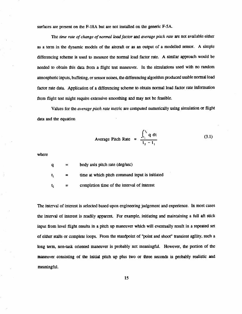
Values for the average pitch rate metric are computed numerically using simulation or flight

data and the equation

where

q =

t 1 =

t2 =

Average Pitch Rateft t2I qdt

t 2 - t 1

(3A)

body axis pitch rate (deg/sec)

time at which pitch command input is initiated

completion time of the interval of interest

The interval of interest is selected based upon engineering judgement and experience. In most cases

the interval of interest is readily apparent. For example, initiating and maintaining a full aft stick

input from level flight results in a pitch up maneuver which will eventually result in a repeated set

of either stalls or complete loops. From the standpoint of "point and shoot" transient agility, such a

long term, non-task oriented maneuver is probably not meaningful. However, the portion of the

maneuver consisting of the initial pitch up plus two or three seconds is probably realistic and

meaningful.

15

ThegeneticF-18A simulation is used to assess the sensitivity of the pitch agility metrics. It

is important to note that these sensitivity results are specific to the generic F-18A only, and cannot

be generalized to all fighter aircraft. The intent here is simply to determine in a broad sense how

sensitive the pitch agility metrics can be to pilot inputs, and to demonstrate one way in which an

analysis of this type can be conducted. If Figure 3.1 represents the nominal pilot command input, then

the actual pilot command input can deviate from the nominal in the following ways (REF. 1):

.

2.

3.

4.

The initial aft stick input can be applied at a slower rate.

The aft stick input can be less than a full deflection command.

The forward stick input can be applied at a slower rate.

The magnitude of the forward stick input may be too large.

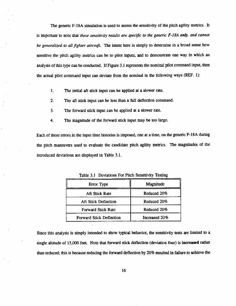
Each of these errors in the input time histories is imposed, one at a time, on the generic F-18A during

the pitch maneuvers used to evaluate the candidate pitch agility metrics. The magnitudes of the

introduced deviations are displayed in Table 3.1.

Table 3.1 Deviations For Pitch Sensitivity Testing

Error Type II Magnitude

Aft Stick Rate Reduced 20%

Aft Stick Deflection Reduced 20%

Forward Stick Rate Reduced 20%

Forward Stick Deflection Increased 20%

Since this analysis is simply intended to show typical behavior, the sensitivity tests are limited to a

single altitude of 15,000 feel Note llmt forward stick deflection (deviation four) is Increased rather

than reduced; this is because reducing the forward deflection by 20% resulted in failure to achieve the

16

zeronormal load factor as required by the metric definitions.

Not all of the input errors listed in Table 3.1 will affect both the pitch up and pitch down

portions of the test maneuver. Only the aft stick command deviations (one and two) influence the

time to maximum normal load factor, positive normal load factor rate, and maximum positive pitch

rate metrics. Considering the pitch down portion of the metrics, only the aft stick command rate

(deviation one) is not influential since the rate at which the initial nose up command is applied has

no effect on the pitch down maneuvers. However, the magnitude of the initial aft stick deflection

(deviation two) does affect the attitude from which the pitch down is initiated.

3.4 CANDIDATE PITCH AGILITY METRICS RESULTS

In this section each of the eight pitch agility metrics will be presented. Each metric is defined and

then typical results are presented.

3.4.1 Maximum Positive Pitch Rate (REF. 18)

3.4.1.1 Definition

The maximum value of positive pitch rate attainable in transitioning from a lg flight

condition to maximum lift angle of attack.

3.4.1.2 Discussion and Typical Results

The maximum positive pitch rates for the generic F-5A, F-16A, and F-18A from steady level

lg flight are displayed in Figures 3.2, 3.3, and 3.4. Maximum aft stick deflections are used for the

generic F-16A and genetic F-18A since the full authority flight control systems on these aircraft

prevent overstressing of the airframe. Since the generic F-5A does not have a full authority flight

control system, the magnitude of the aft stick deflections must be selected to prevent overstressing.

17

............i..........................i......................i.............i.............i.............i............i.............i80 ...........i............i..........: .........i............i.............i............i............i.............

'_ 40 .........:.............: i ......i............i

it i ii i i i i !iiiiiiiii" i...............ZZ ZIIIiiiZZIIIZI iiiZZIIZ iiZZIII ZIII....I0.4 0.5 0.6 0.7 0.8 0.9

Mach number ---o---F-SAF-16A

F-IgA

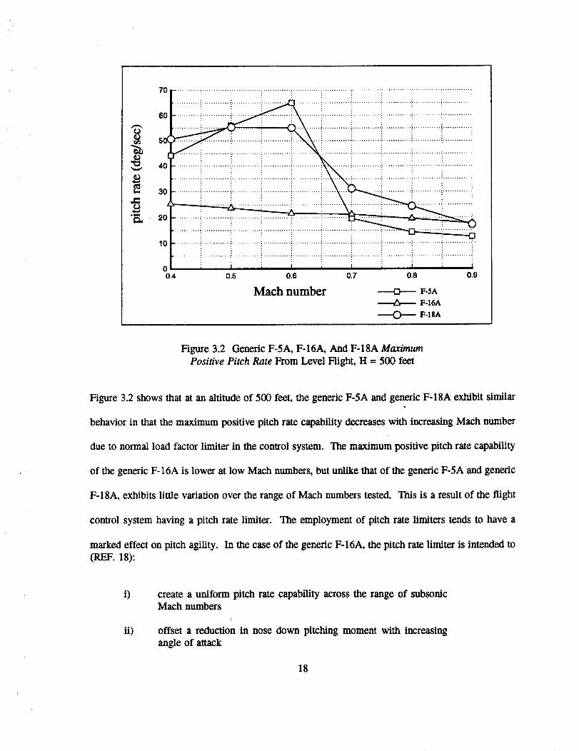
Figure 3.2 Generic F-5A, F-16A, And F-18A Max/mum

Positive Pitch Rate From Level Flight, H = 500 feet

Figure 3.2 shows that at an altitude of 500 feet, the generic F-5A and generic F-18A exhibit similar

behavior in that the maximum positive pitch rate capability decreases with increasing Mach number

due to normal load factor limiter in the control system. The maximum positive pitch rate capability

of the generic F-16A is lower at low Mach numbers, but unlike that of the generic F-5A and generic

F-18A, exhibits little variation over the range of Mach numbers tested. This is a result of the flight

control system having a pitch rate limiter. The employment of pitch rate limiters tends to have a

marked effect on pitch agility. In the case of the generic F-16A, the pitch rate limiter is intended to(REF. 18):

i)

ti)

create a uniform pitch rate capability across the range of subsonicMach numbers

offset a reduction in nose down pitching moment with increasing

angle of attack

18

iii) avoid a deep stall tendency

The maximum positive pitch rate capability for the three aircraft at an altitude of 15,000 feet

is displayed in Figure 3.3.

70 .......................... "....................................... _ ............. : ........................... _ ............ _ ............. :

! ! . i............!............i.............!............. !.............

t "

40

30 !

lo ..........i.............i.............i............i...........i............i.............i............i............i............i

o ..........i..........................i............i..........i.............i..........................i............i.............0.4 0.5 0.6 0.7 0.8 O.g

Mach number ------m---- F-s,.,F-16A

------O-- F-lSA

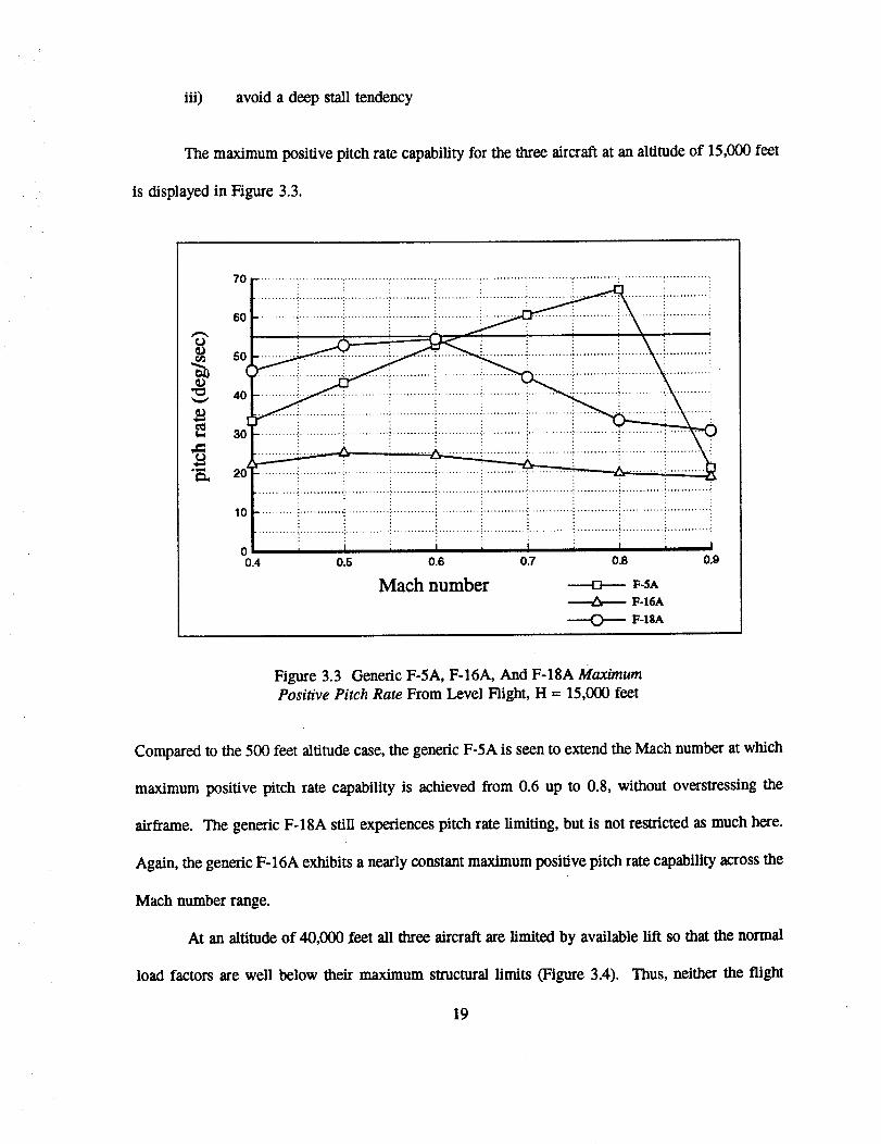
Figure 3.3 Generic F-5A, F-16A, And F-18A MaximumPositive Pitch Rate From Level Flight, H = 15,000 feet

Compared to the 500 feet altitude case, the generic F-5A is seen to extend the Mach number at which

maximum positive pitch rate capability is achieved from 0.6 up to 0.8, without overstressing the

airframe. The generic F-18A still experiences pitch rate limiting, but is not restricted as much here.

Again, the generic F-16A exhibits a nearly constant maximum positive pitch rate capability across the

Mach number range.

At an altitude of 40,000 feet all three aircraft are limited by available lift so that the normal

load factors are well below their maximum structural limits (Figure 3.4). Thus, neither the flight

19

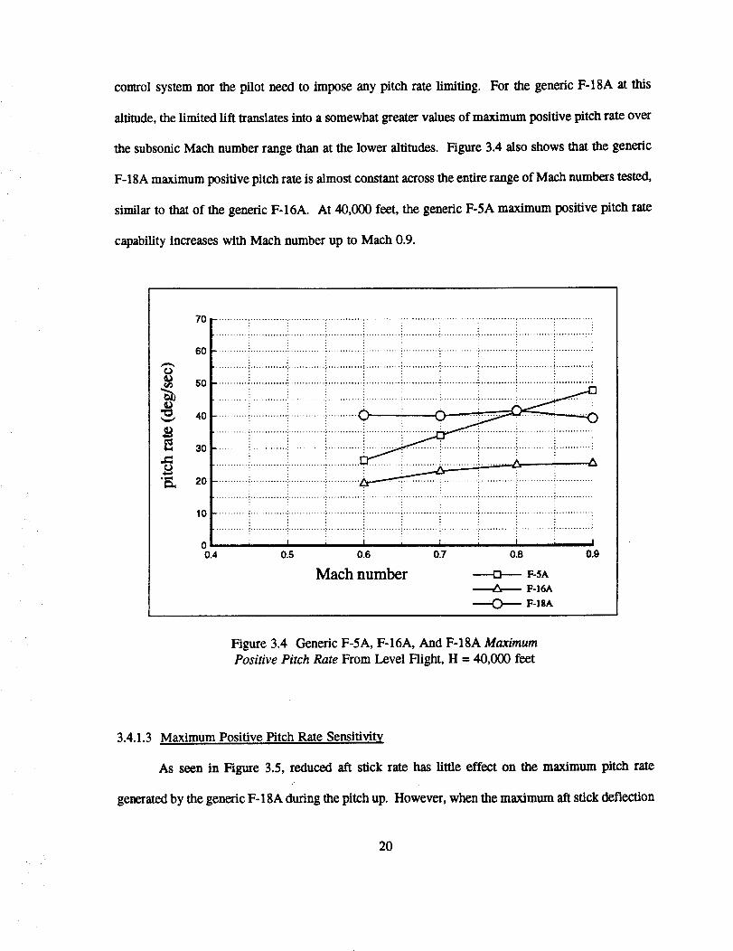
controlsystemnor thepilot needto imposeanypitchratelimiting. ForthegenericF-18Aat this

altitude,thelimited lift translates into a somewhat greater values of maximum positive pitch rate over

the subsonic Mach number range than at the lower altitudes. Figure 3.4 also shows that the generic

F-18A maximum positive pitch rate is almost constant across the entire range of Math numbers tested,

similar to that of the generic F-16A. At 40,000 feet, the generic F-SA maximum positive pitch rate

capability increases with Mach number up to Mach 0.9.

I._ :

so ..........._.......................................::............i ............i..........................i ............,............

........... _............. :............. , ............ i ............ :............. ::........................... ; ............ :............. ::

_o ...........i............i.............i ............i............i............i.........................._............i............-! : :

.......................... :............. : ............ : ............ :............. :........................... i ............ :............. i

0 I I i I i I i l i I0.4 o.s 0.6 0.7 o.a o._

Mach number ---m--- F-SAF-16A

F-18A

Figure 3.4 Generic F-5A, F-I6A, And F-18A Maximum

Positive Pitch Rate From Level Flight, H = 40,000 feet

3.4.1.3 Maximum Positive Pitch Rate Sensitivity

As seen in Figure 3.5, reduced aft stick rate has little effect on the maximum pitch rate

generated by the generic F-18A during the pitch up. However, when the maximum aft stick deflection

20

70

60

50(

4Oq

3O

2O

10

00.4

........... . ............. i.......................... i .......................... :........................................ i ............. :

i!!!iii !!iiii::!::iii!!i!ii !ii!ii i

............!............i.............i...........i............i.............i.............i............_............i............

...........i.............i.............i............i............_.............i.............i..........................i.............

............!.............!.............!............!............!.............!.............!..........i ............!.............i I i I = I i I i I

0.5 0.6 0.7 0.8 0.9

Mach number ----O--- ,om_=f¢ s_ r_ error

aft _ magnitu_ _ror

Figure 3.5 Generic F-18A Maximum Positive Pitch Rate Sensitivity, H = 15,000 feet

is reduced 20%, the maximum positive pitch rate is significantly reduced in the range of lower Mach

numbers. This deviation tends to have a pronounced effect on maximum positive pitch rate, but little

to no impact on the other metrics. This is because the value of each different pitch agility metric is

established at a different point in the time history of the maneuver. For example, maximum positive

normal load factor rate occurs very early in the maneuver, at a time when maximum positive pitch

rate is still relatively small. Also, the peak positive normal load factor is achieved later in the

maneuver, when normal load factor rate is zero, and after positive pitch rate has peaked and is

declining.

21

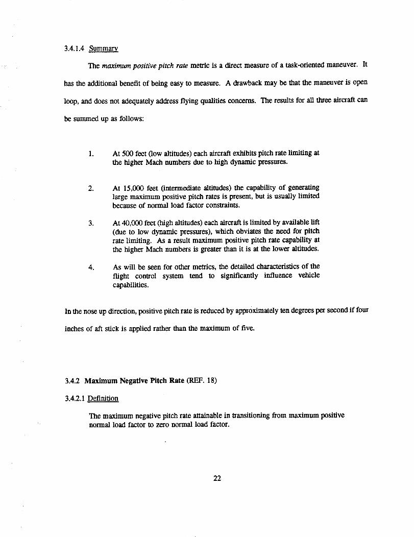
3.4.1.4 Summary

The maximum positive pitch rate metric is a direct measure of a task-oriented maneuver. It

has the additional benefit of being easy to measure. A drawback may be that the maneuver is open

loop, and does not adequately address flying qualities concerns. The results for all three aircraft can

be summed up as follows:

o At 500 feet (low altitudes) each aircraft exhibits pitch rate limiting at

the higher Mach numbers due to high dynamic pressures.

.

.

.

At 15,000 feet 0ntermediate altitudes) the capability of generating

large maximum positive pitch rates is present, but is usually limitedbecause of normal load factor constraints.

At 40,000 feet (high altitudes) each aircraft is limited by available lift

(due to low dynamic pressures), which obviates the need for pitch

rate limiting. As a result maximum positive pitch rate capability at

the higher Mach numbers is greater than it is at the lower altitudes.

As will be seen for other metrics, the detailed characteristics of the

flight control system tend to significantly influence vehicle

capabilities.

In the nose up direction, positive pitch rate is reduced by approximately ten degrees per second if four

inches of aft stick is applied rather than the maximum of five.

3.4.2 Maximum Negative Pitch Rate (REF. 18)

3.4.2.1 Definition

The maximum negative pitch rate attainable in transitioning from maximum positivenormal load factor to zero normal load factor.

22

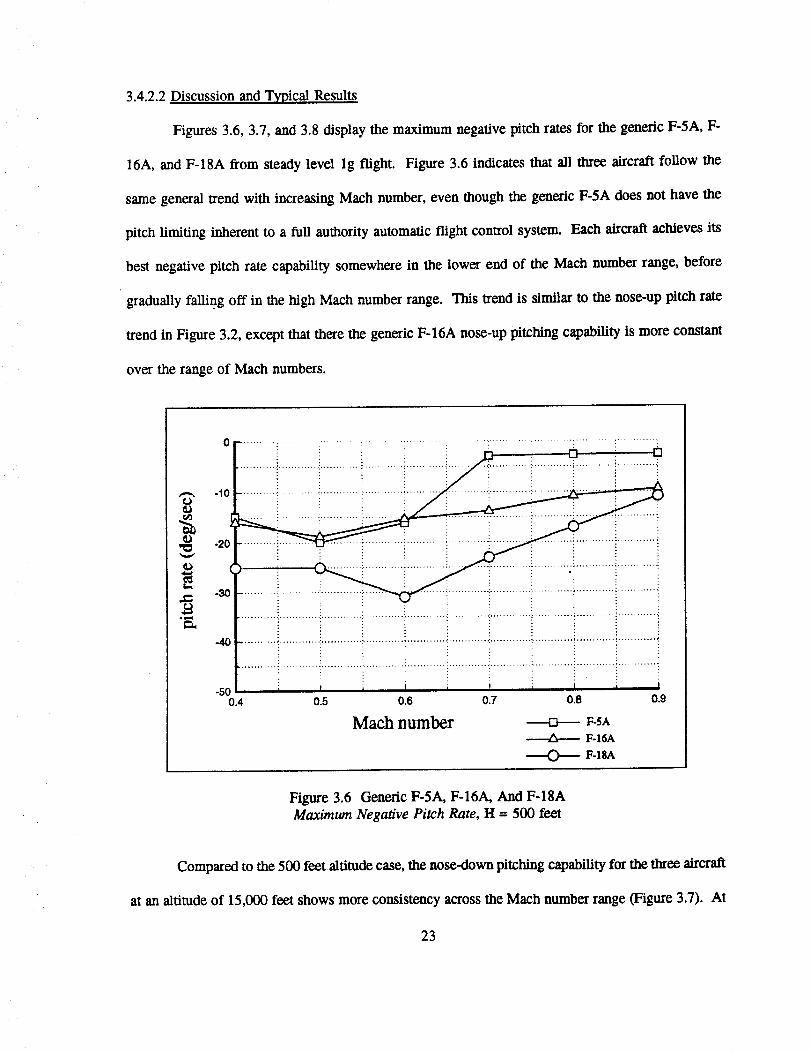
3.4.2.2 Discussion and Typical Results

Figures 3.6, 3.7, and 3.8 display the maximum negative pitch rates for the generic F-5A, F-

16A, and F-18A from steady level lg flight. Figure 3.6 indicates that all three aircraft follow the

same general trend with increasing Mach number, even though the generic F-SA does not have the

pitch limiting inherent to a full authority automatic flight control system. Each aircraft achieves its

best negative pitch rate capability somewhere in the lower end of the Mach number range, before

gradually falling off in the high Mach number range. This trend is similar to the nose-up pitch rate

trend in Figure 3.2, except that there the generic F-16A nose-up pitching capability is more constant

over the range of Mach numbers.

-10

-20

O

.N

-40

-5C0.4

! i ! !

?, I , I i I i I i I0.5 0.6 0.7 0.8 0.9

Maeh number F-SAF-16A

F-hA

Figure 3.6 Generic F-5A, F-16A, And F-18A

Maximum Negative Pitch Rate, H = 500 feet

Compared to the 500 feet altitude case, the nose-down pitching capability for the three aircraft

at an altitude of 15,000 feet shows more consistency across the Math number range (Figure 3.7). At

23

this altitude there is also a greater disparity between the three aircraft. The generic F-16A and generic

F-18A once again exhibit the effects of pitch limiting, but in terms of magnitude the generic F-18A

nose-down pitch capability is actually better at this altitude. The generic F-16A capability at this

altitude is virtually unchanged from the lower altitude, both in terms of magnitude and trend with

Mach number. As is the case for nose-up pitch rate capability on the generic F-5A, increasing altitude

has the effect of extending the Mach number at which maximum negative pitch rate capability is

achieved.

.l,m

-40 ......................... _........................... r............ ; ............ ! ............. _............ !.........................

! ! : : :

-so , i i i i i i0.4 o.s 0.6 0.7 o.0

Mach number

0.8

P-SA

F-16A

F-lSA

Figure 3.7 Generic F-5A, F-16A, And F-18A

Maximum Negative Pitch Rate, H -- 15,000 feet

At an altitude of 40,000 feet neither the Right conl_ol system nor the pilot need to impose any

pitch rate limiting. Figure 3.8 shows very little change over Figure 3.7, except that the genetic F-5A

has a nearly constant negative pitch rate capability across the Math number range like the other two

24

aircraft.ThegenericF-18Ahasaslightlygreaternegative pitch rate capability at this altitude than

it does at the lower altitudes.

•_ -20

.3o

0 ......... • ............ •.......... •............. ' ......... ' ..... :......... "............ " .......... " ......

-10 ....................................... . ............ ' ...................................................... !............ _............

-40 ........... ;............. !............. ; ............................................................................... _............

-50 ) i I i I I i0.4 0.5 0.7 0.8 0.9

i t )0.6

Mach number F-SA

F-16A

0 F-18A

Figure 3.8 Generic F-5A, F-16A, And F-18A

Maximum Negative Pitch Rate, H = 15,000 feet

3.4.2.3 Maximum Negative Pitch Rate Sensitivity

The sensitivity of the maximum negative pitch rate metric to deviations in forward stick rate,

aft stick magnitude and forward stick magnitude for the generic F-18A are shown in Figure 3.9. It

is seen that commanding more than the nominal forward stick deflection causes slightly larger negative

pitch rates, while applying the stick input at a slower rate reduces the magnitude of the resulting pitch.

In no case, however, are the changes large or unpredictable.

25

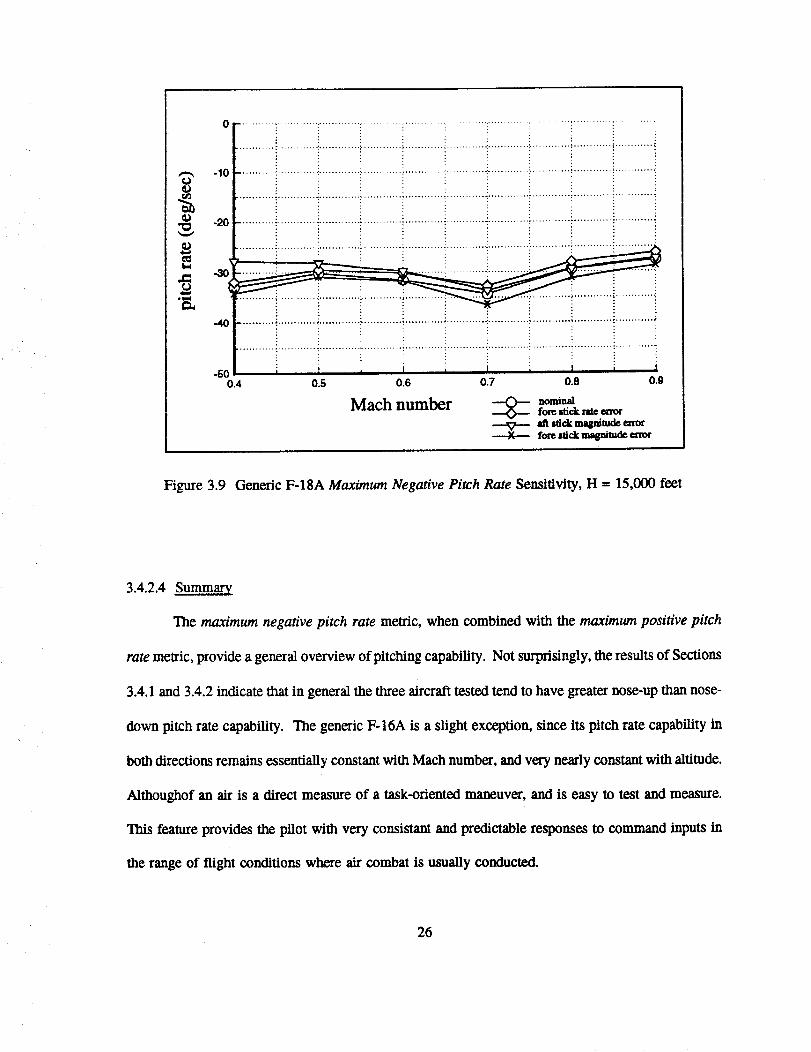
_'_ -10

_ -20

-500.4

........... . ........... .............. ............. , ........... , ....... ............. . .................. : ....... ,

...........'............_.............i............'.........................i..........................i.........................i

.........................i............."......................................i............._............i.........................?i I , I , I i I i I

0.5 0.6 0.7 0.8 0.9

Mach number ::_ ,o_._aforesfek rate errorV

_t .tick magnituck _rorforestickmagnitudeegror

Figure 3.9 Generic F-18A Maximum Negative Pitch Rate Sensitivity, H = 15,000 feet

3.4.2.4 Summary

The maximum negative pitch rate metric, when combined with the maximum positive pitch

rate metric, provide a general overview of pitching capability. Not surprisingly, the results of Sections

3.4.1 and 3.4.2 indicate that in general the three aircraft tested tend to have greater nose-up than nose-

down pitch rate capability. The generic F-16A is a slight exception, since its pitch rate capability in

both directions remains essentially constant with Mach number, and very nearly constant with altitude.

Althoughof an air is a direct measure of a task-oriented maneuver, and is easy to test and measure.

This feature provides the pilot with very consistant and predictable responses to command inputs in

the range of flight conditiom where air combat is usually conducted.

26

Maximum Positive And Negative Pitch Rate From An Initial Angle Of Attack

Definition

The maximum positive or negative pitch rate attained from pitching up or down from

a specified initial angle of attack.

3.4.3.2 Discussion and Typical Results

If maximum positive and negative pitch rates are used to quantify pitch agility, then the flight

maneuver used previously is not adequate to fully evaluate this capability. A full deflection aft stick

input followed by pitch down to zero load factor results in pitch rate data at only one angle of attack

for each flight condition. A more complete picture would show pitch rate versus initial angle of attack

at representative flight conditions. A proposed flight test maneuver consists of pitching the aircraft

with incremental longitudinal stick inputs. Then full aft (or forward if nose down rates are being

studied) stick is applied. Maximum pitch rate is recorded and plotted against the angle of attack from

which the maximum rate command was initiated. The full deflection inputs should follow the initial

incremental steps quickly enough that aircraft Mach and altitude remain within acceptable flight test

tolerances.

The simulation results from this procedure using the generic F-18A at 15,000 feet is shown

in Figure 3.10. The trends for each Mach number show that as the initial angle of attack is increased,

the pitching moment authority remaining available to generate nose up pitch rate is reduced. Figure

3.10 shows the effect of the flight control system limiting the pitch rates at Math equals 0.8 to prevent

the generic F-18A from exceeding its structural limit. At Mach equals 0.4 and 0.6 at an altitude of

15,000 feet, because the value of maximum lift will not overstress the aircraft, there is no need to

limit the pitch rate.

27

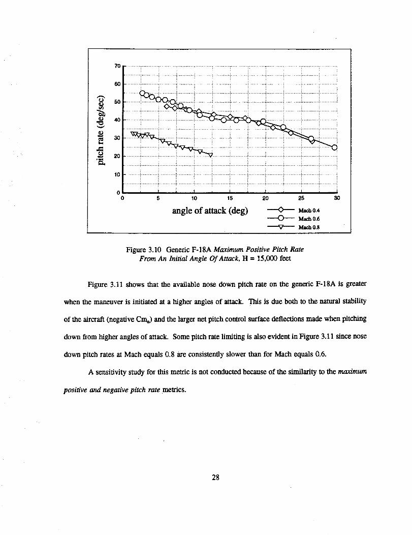
70

60

50

40

N 2o

10

00

!.........i..........i..........i..........i.........!..........i.........._..........i..........;...........i..........i...........i......... i .......... i.......... i .......... ::.......... i.......... _.......... :.......... _.......... _.......... !.......... i........... i

.........i..........i..........i..........i..........i..........i.....................i..........i..........i..........i..........

i I i I i I i I i I i I5 10 15 20 25 30

angle of attack (deg) ----O--- M_ 0.4---O---- M_a 0.6

Ml_a 0.S

Figure 3.10 Generic F-18A Maximum Positive Pitch Rate

From An Initial Angle Of Attack, H = 15,000 feet

Figure 3.11 shows that the available nose down pitch rate on the generic F-18A is greater

when the maneuver is initiated at a higher angles of attack. This is due both to the natural stability

of the aircraft (negative Cm_) and the larger net pitch control surface deflections made when pitching

down from higher angles of attack. Some pitch rate limiting is also evident in Figure 3.11 since nose

down pitch rates at Mach equals 0.8 are consistently slower than for Mach equals 0.6.

A sensitivity study for this metric is not conducted because of the similarity to the max/mum

positive and negative pitch rate metrics.

28

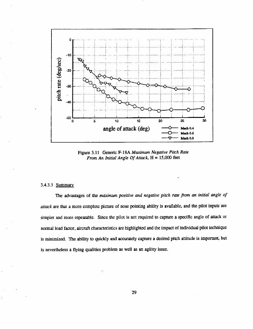
0 ............. ' ........ •

-10

-20

-500

......... i ..................... _ .......... ' .......... t .......... : .......... : ...........................................

.i:i .......i,.i! H.i I I I i I i I i t i I

5 10 15 20 25 30

angle of attack (deg) --0-- _ 0.4------0--- M,_ o.6

Figure 3.11 Generic F-18A Maximum Negative Pitch Rate

From An Initial Angle Of Attack, H = 15,000 feet

3.4.3.3 Summary

The advantages of the max/mum positive and negative pitch rate from an initial angle of

attack are that a more complete picture of nose pointing ability is available, and the pilot inputs are

simpler and more repeatable. Since the pilot is not required to capture a specific angle of attack or

normal load factor, aircraft characteristics are highlighted and the impact of individual pilot technique

is minimized. The ability to quickly and accurately capture a desired pitch attitude is important, but

is nevertheless a flying qualities problem as well as an agility issue.

29

3.4.4Time To Pitch To Maximum Positive Normal Load Factor (REF. 18)

3.4.4.1 Definition

The sum of:

time to pitch from a lg flight condition to maximum lift coefficient or normal loadfactor

and

time to pitch down from maximum lift coefficient or normal load factor to Og

3.4.4.2 Discussion and Typical Results

This definition of pitch agility correctly implies that both nose up and nose down pitch agility are

important. There are, however, a number of questions this definition raises including:

.

.

.

If the times associated with nose up and nose down pitch maneuvers

are to be summed, should the two be equally weighted?

Is the time to pitch up significantly different than the time to pitchdown?

Does an aircraft with better positive pitch agility necessarily have

better negative pitch agility?

Since these questions remain to be resolved by the engineering and pilot communities, in the current

research values of this metric associated with nose up pitch maneuvers are treated separately from

values associated with nose down pitch maneuvers. The nose up pitch maneuver is the t/me to pitch

up to maximum normal load factor and the nose down pitch maneuver is the time to pitch down from

maximum normal load factor to Og.

Figures 3.12, 3.13, and 3.14 show that the time to pitch up to maximum normal load factor

is a strong function of Mach number and altitude. For the generic F-5A at the altitudes tested, normal

acceleration due to angle of attack tends to increase with increasing Math number. The resulting time

to load is smaller, even in cases where the pitch rates at each Math number are nearly the same.

30

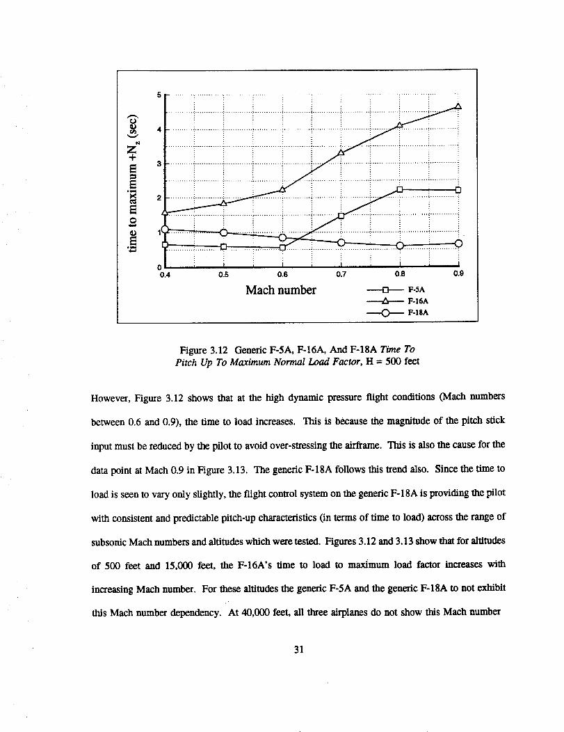
O

Z4-E

E.N

E

E

00.4

................................................. i................ i

i i i i i :: i _i I i t i I , I , I

0.5 0.6 0.7 0.8 0.9

Mach number ---o--- F-_AF-16A

----0--- F-hA

Figure 3.12 Generic F-5A, F-16A, And F-18A Time To

Pitch Up To Maximum Normal Load Factor, H = 500 feet

However, Figure 3.12 shows that at the high dynamic pressure flight conditions (Math numbers

between 0.6 and 0.9), the time to load increases. This is because the magnitude of the pitch stick

input must be reduced by the pilot to avoid over-stressing the airframe. This is also the cause for the

data point at Mach 0.9 in Figure 3.13. The generic F-18A follows this trend also. Since the time to

load is seen to vary only slightly, the flight control system on the generic F-18A is providing the pilot

with consistent and predictable pitch-up characteristics On terms of time to load) across the range of

subsonic Mach numbers and altitudes which were tested. Figures 3.12 and 3.13 show that for altitudes

of 500 feet and 15,000 feet, the F-16A's time to load to maximum load factor increases with

increasing Mach number. For these altitudes the generic F-5A and the generic F-18A to not exhibit

this Math number dependency. At 40,0130 feet, all three airplanes do not show this Mach number

31

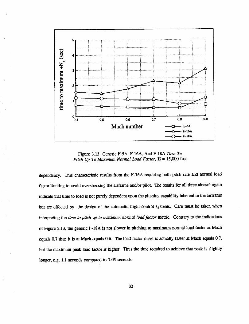
t4

z

E

E t D

0 i 1 i I i I I I i I0.4 0.5 0.6 0.7 0.8 0.0

Mach number --o--- F-_^F-16A

O F-ISA

Figure 3.13 Generic F-5A, F-16A, And F-18A Time To

Pitch Up To Maximum Normal Load Factor, H = 15,000 feet

dependency. This characteristic results from the F-16A requiting both pitch rate and normal load

factor limiting to avoid overstressing the airframe and/or pilot. The results for all three aircraft again

indicate that time to load is not purely dependent upon the pitching capability inherent in the airframe

but are effected by the design of the automatic flight control systems. Care must be taken when

interpreting the time to pitch up to maximum normal load factor metric. Contrary to the indications

of Figure 3.13, the generic F-18A is not slower in pitching to maximum normal load factor at Mach

equals 0.7 than it is at Mach equals 0.6. The load factor onset is actually faster at Math equals 0.7,

but tiae maximum peak load factor is higher. Thus the time required to achieve that peak is slightly

longer, e.g. 1.1 seconds compared to 1.05 seconds.

32

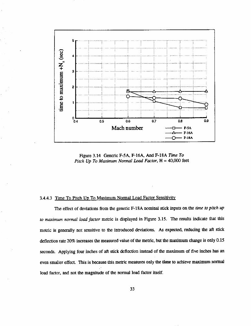
N

z3

00.4

: i !.................................................................i............!.............: ............!............:.............

........................i..........................!.........................._............._.............i ............i............_i 1 i I i f i I i I

o.s 0.6 0.7 0.8 0.9

Mach number -----o---- F-SAF-16A

-----O-- F-is^

Figure 3.14 Generic F-5A, F-16A, And F-18A Time To

Pitch Up To Maximum Normal Load Factor, H = 40,000 feet

3.4.4.3 Time To Pitch Up To Maximum Normal Load Factor Sensitivi .ty

The effect of deviations from the generic F-18A nominal stick inputs on the time to pitch up

to maximum normal load factor metric is displayed in Figure 3.15. The results indicate that this

metric is generally not sensitive to the introduced deviations. As expected, reducing the aft stick

deflection rate 20% increases the measured value of the metric, but the maximum change is only 0.15

seconds. Applying four inches of aft stick deflection instead of the maximum of five inches has an

even smaller effect. This is because this metric measures only the time to achieve maximum normal

load factor, and not the magnitude of the normal load factor itself.

33

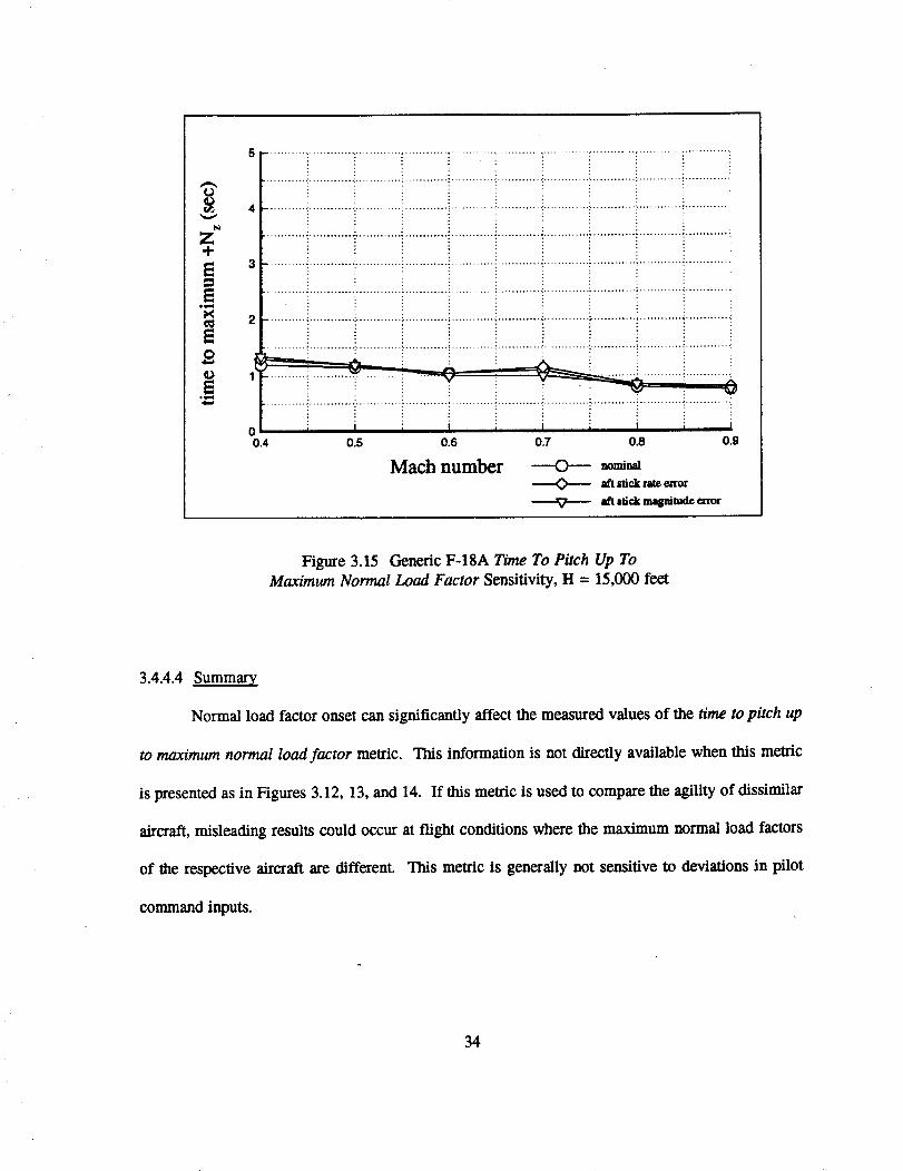
t3

t_

z

21_

00.4

............_........................................i .........................!..........................!............!............!

............i.......................................!.........................i..........................i............i.............i I ; I i I i I I I

0.5 0.6 0.7 0.8 0.9

Mach number ---<>-- _o__ _ck r_ error

_ s_c_ nuqlnimde e_mr

Figure 3.15 Generic F-18A Time To Pitch Up ToMaximum Normal Load Factor Sensitivity, H = 15,000 feet

3.4.4.4 Summary

Normal load factor onset can significantly affect the measured values of the t/me to pitch up

to maximum normal load factor metric. Tiffs information is not directly available when this metric

is presented as in Figures 3.12, 13, and 14. If this metric is used to compare the agility of dissimilar

aircraft, misleading results could occur at flight conditions where the maximum normal load factors

of the respective aircraft are different. This metric is generally not sensitive to deviations in pilot

command inputs.

34

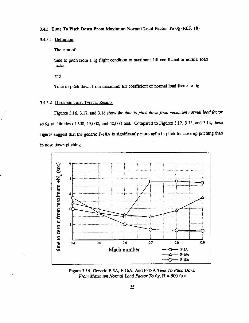
3.4.5 Time To Pitch Down From Maximum Normal Load Factor To 0g (REF. 18)

3.4.5.1 Definition

The sum of:

time to pitch from a lg flight condition to maximum lift coefficient or normal loadfactor

and

Time to pitch down from maximum lift coefficient or normal load factor to 0g

3.4.5.2 Discussion and Typical Results

Figures 3.16, 3.17, and 3.18 show the time to pitch down from maximum normal load factor

to Og at altitudes of 500, 15,000, and 40,000 feet. Compared to Figures 3.12, 3.13, and 3.14, these

figures suggest that the generic F-18A is significantly more agile in pitch for nose up pitching than

in nose down pitching.

_, 5

1,4

z.

O00.4

........... • ............. .............. o ............ . ............. . ............ . ............. • ............ : ............ , .............

.?

i I i [ i I i I i I0.5 0.6 0.7 0.8 o.g

Mach number F-SAF-16A

----O--- F-lSA

Figure 3.16 Generic F-5A, F-16A, And F-18A Time To Pitch Down

From Maximum Normal Load Factor To Og, H = 500 feet

35

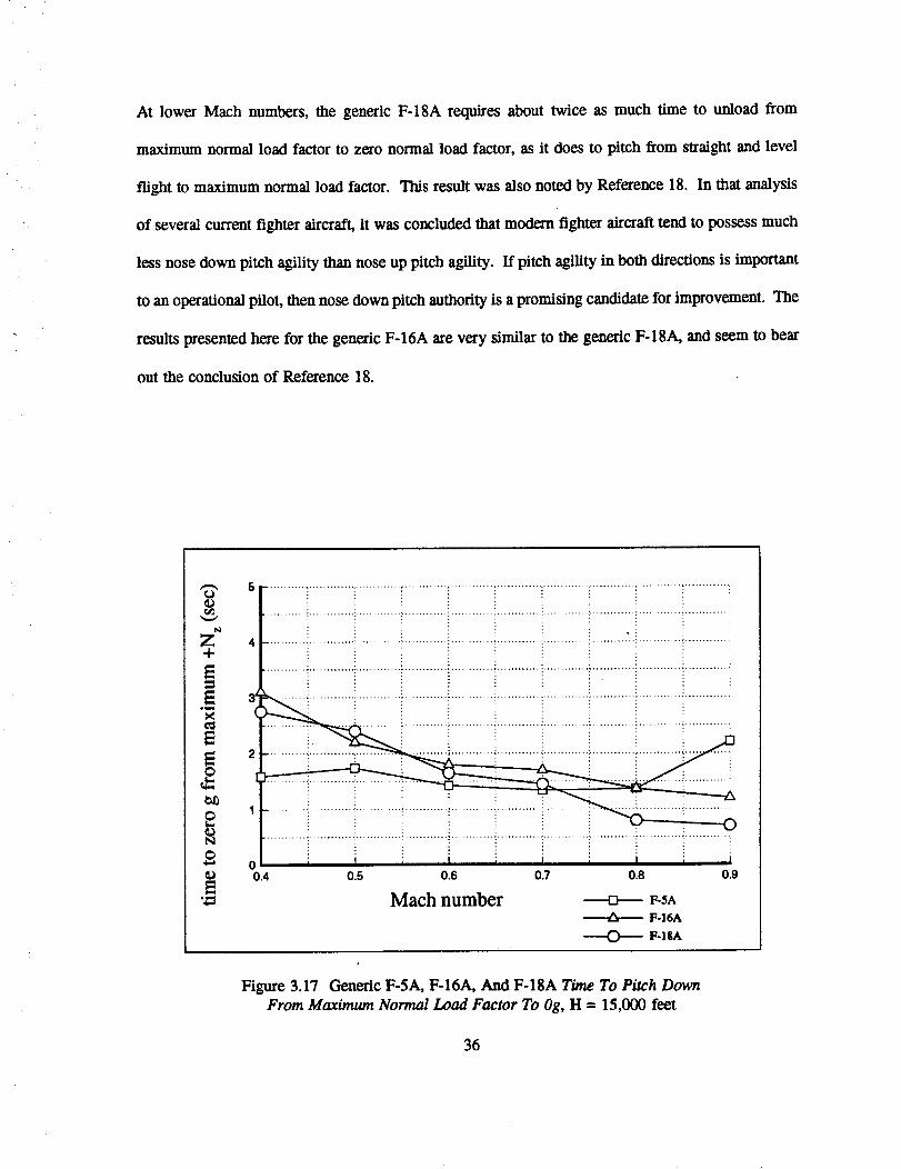
At lower Mach numbers, the generic F-18A requires about twice as much time to unload from

maximum normal load factor to zero normal load factor, as it does to pitch from straight and level

flight to maximum normal load factor. This result was also noted by Reference 18. In that analysis

of several current tighter aircraft, it was concluded that modem tighter aircraft tend to possess much

less nose down pitch agility than nose up pitch agility. If pitch agility in both directions is important

to an operational pilot, then nose down pitch authority is a promising candidate for improvement. The

results presented here for the generic F-16A are very similar to the generic F-18A, and seem to bear

out the conclusion of Reference 18.

z4-

¢_

O

¢x0

o

O4.0

5 ........... ".............. " ............ " ............ ' ............ ' ............. " ............. ' ............. : ............ "..............

4 ..................................................................................................... ?i ......................... !

..........i.....................................................................................................................i

......................... i.......................... ! ............ !............ _........................... ! ............ !............

0 , I I i I i I0.4 0.5 0.7 0.8 0.9

.I i

0.6

Mach number F-SA

F-16A

F-_SA

Figure 3.17 Generic F-5A, F-16A, And F-18A Time To Pitch Down

From Maximum Normal Load Factor To Og, H = 15,000 feet

36

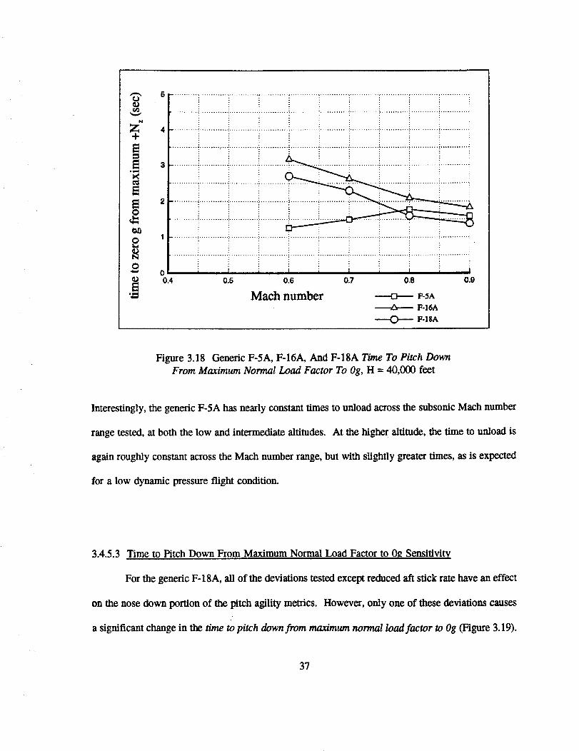
z4-

O

o

o00.4

iiiliiiiiiiiiiiiiiiiiii ....i i i i

I i I i I i I i io.s o.e o.z o.e o._

Mach number _ F-SAF-16A

F-lS^

Figure 3.18 Generic F-5A, F-16A, And F-18A Time To Pitch Down

From Maximum Normal Load Factor To Og, H = 40,000 feet

Interestingly, the generic F-5A has nearly constant times to unioad across the subsonic Mach number

range tested, at both the low and intermediate altitudes. At the higher altitude, the time to unload is

again roughly constant across the Mach number range, but with slightly greater times, as is expected

for a low dynamic pressure flight condition.

3.4.5.3 Time to Pitch Down From Maximum Normal Load Factor to 0g Sensitivity

For the generic F-18A, all of the deviations tested except reduced aft stick rate have an effect

on the nose down portion of the pitch agility metrics. However, only one of these deviations causes

a significant change in the time to pitch down from maximum normal load factor to Og (Figure 3.19).

37

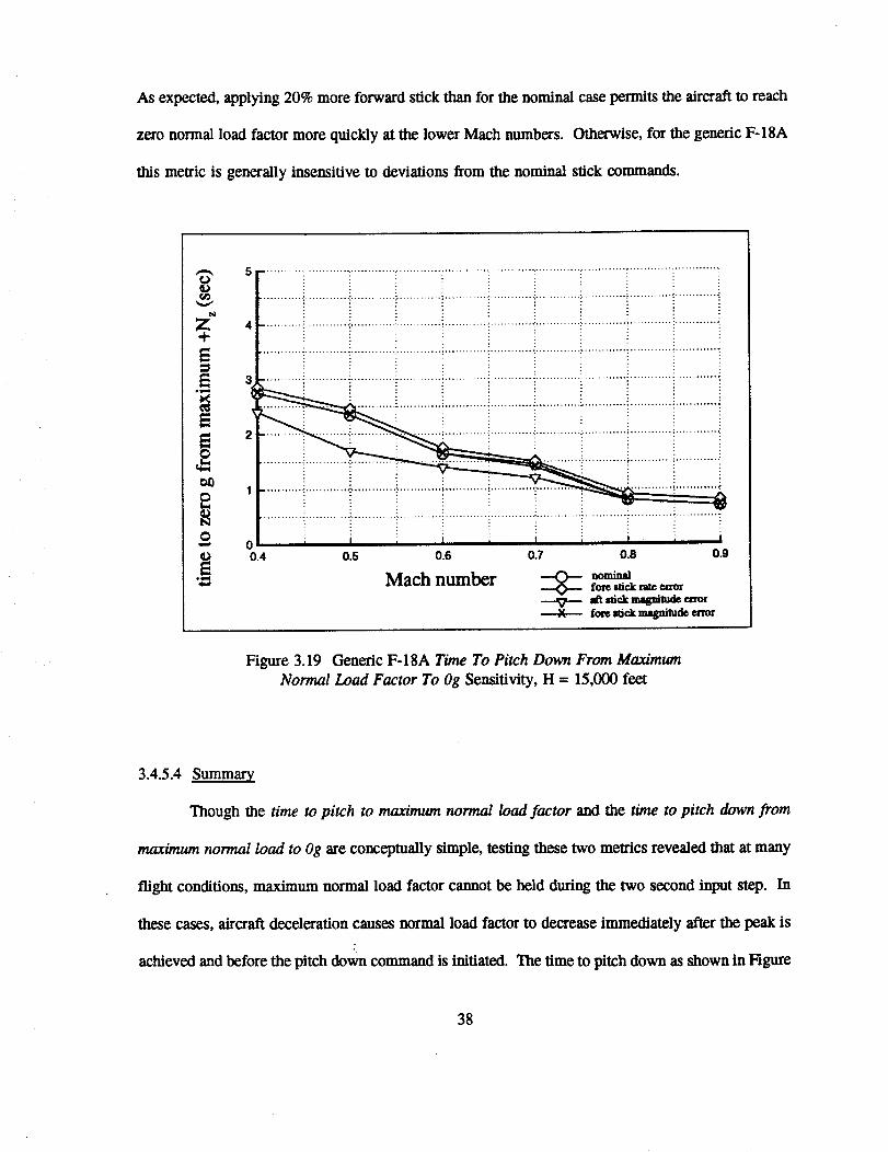
Asexpected, applying 20% more forward stick than for the nominal case permits the aircraft to reach

zero normal load factor more quickly at the lower Mach numbers. Otherwise, for the genetic F-18A

this medic is generally insensitive to deviations from the nominal stick commands.

t_

N

z

i

O r I i I i I i t I I0.4 o.5 o.6 o.7 o.e o.9

Mach number _ ,om=_fore Ilick rate _ttotv

_ _iek mqnim_ euorfore _it_k m_aim_ error

Figure 3.19 Genetic F-18A Time To Pitch Down From Maximum

Normal Load Factor To Og Sensitivity, H = 15,000 feet

3.4.5.4 Summary

Though the t/me to pitch to maximum normal load factor and the time to pitch down from

maximum normal load to Og are conceptually simple, testing these two metrics revealed that at many

flight conditions, maximum normal load factor cannot be held during the two second input step. In

these cases, aircraft deceleration causes normal load factor to decrease immediately after the peak is

achieved and before the pitch down command is initiated. The time to pitch down as shown in Figure

38

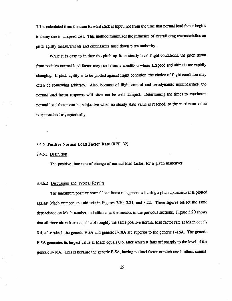
3.1 is calculated from the time forward stick is input, not from the time that normal load factor begins

to decay due to airspeed loss. This method minimizes the influence of aircraft drag characteristics on

pitch agility measurements and emphasizes nose down pitch authority.

While it is easy to initiate the pitch up from steady level flight conditions, the pitch down

from positive normal load factor may start from a condition where airspeed and altitude are rapidly

changing. If pitch agility is to be plotted against flight condition, the choice of flight condition may

often be somewhat arbitrary. Also, because of flight control and aerodynamic nonlinearities, the

normal load factor response will often not be well damped. Determining the times to maximum

normal load factor can be subjective when no steady state value is reached, or the maximum value

is approached asymptotically.

3.4.6 Positive Normal Load Factor Rate (REF. 32)

3.4.6.1 Definition

The positive time rate of change of normal load factor, for a given maneuver.

3.4.6.2 Discussion and Typical Results

The maximum positive normal load factor rate generated during a pitch up maneuver is plotted

against Mach number and altitude in Figures 3.20, 3.21, and 3.22. These figures reflect the same

dependence on Mach number and altitude as the metrics in the previous sections. Figure 3.20 shows

that all three aircraft are capable of roughly the same positive normal load factor rate at Mach equals

0.4, after which the generic F-5A and generic F-18A are superior to the generic F-16A. The generic

F-5A generates its largest value at Mach equals 0.6, after which it falls off sharply to the level of the

generic F-16A. This is because the generic F-SA, having no load factor or pitch rate limiters, cannot

39

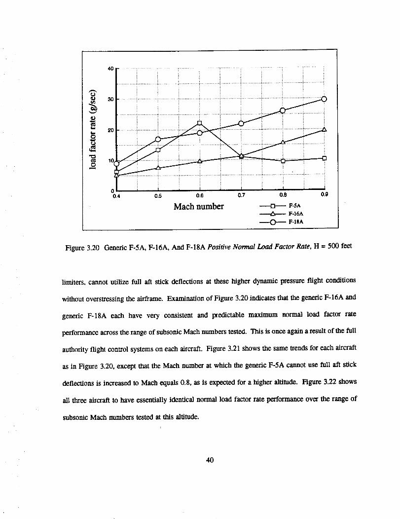
O

401" ........ _.......... : :....... ! ..... _......... i ........ i........... i ........ i ....... i

t ' ' i ' i !30

0.4

........... .. . . .

2O

lo,

i

I I _T I m V , I , Io.s 0.8 0.7 o.e 0.9

Mach number -----cv-- F-SAF-16A

---0--- F-tsA

Figure 3.20 Generic F-5A, F-16A, And F-18A Positive Normal Load Factor Rate, H = 500 feet

limiters, cannot utilize full aft stick deflections at these higher dynamic pressure flight conditions

without overstressing the airframe. Examination of Figure 3.20 indicates that the generic F-16A and

generic F-18A each have very consistent and predictable maximum normal load factor rate

performance across the range of subsonic Mach numbers tested. This is once again a result of the full

authority flight control systems on each aircraft. Figure 3.21 shows the same trends for each aircraft

as in Figure 3.20, except that the Mach number at which the generic F-5A cannot use full aft stick

deflections is increased to Math equals 0.8, as is expected for a higher altitude. Figure 3.22 shows

all three aircraft to have essentially identical normal load factor rate performance over the range of

subsonic Mach numbers tested at this altitude.

J

40

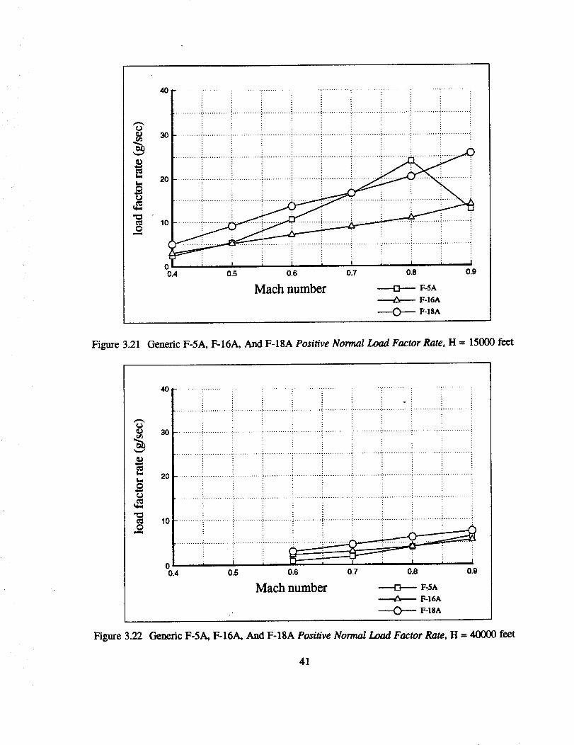
0

0¢-u

°[.............i i............i.........i................i.....i........+ iiiilT !iiiiiii iiiill iliilli ITIi!

20

10

: iI i I I I i I i I

0.4 0.5 0.6 0.7 0.8 0.9

Mach number ----o--- F-SAF-16A

F-1SA

Figure 3.21 Generic F-5A, F-16A, And F-18A Positive Normal Load Factor Rate, H = 15000 feet

40

2o

e==l

..................................................................................................... ?.......................... i

! : !

00.4 0.5 0.6 0.7 0.8 0.9

Mach number -----or--- F,5A

F-16A

.. C) F-18A

Figure 3.22 Generic F-5A, F-16A, And F-18A Positive Normal Load Factor Rate, H = 40000 feet

41

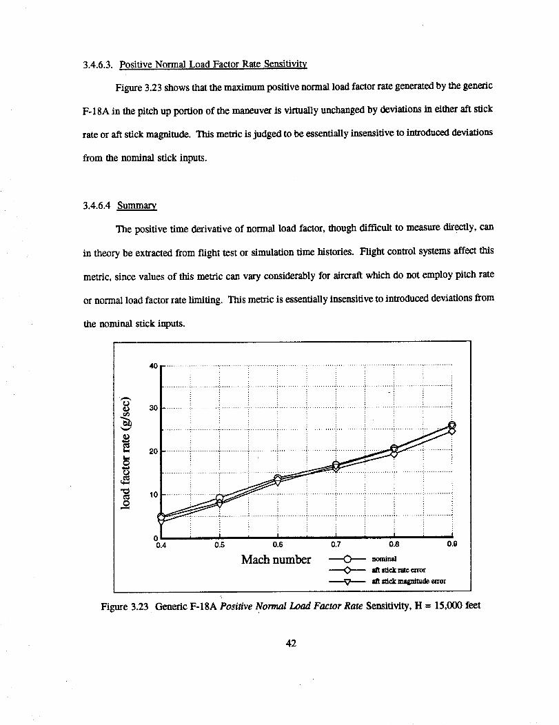
3.4.6.3.Positive Normal Load Factor Rate Sensitivity

Figure 3.23 shows that the maximum positive normal load factor rate generated by the generic

F-18A in the pitch up portion of the maneuver is virtually unchanged by deviations in either aft stick

rate or aft stick magnitude. This metric is judged to be essentially insensitive to introduced deviations

from the nominal stick inputs.

3.4.6.4 Summary

The positive time derivative of normal load factor, though difficult to measure directly, can

in theory be extracted from flight test or simulation time histories. Flight control systems affect this

metric, since values of this metric can vary considerably for aircraft which do not employ pitch rate

or normal load factor rate limiting. This metric is essentially insensitive to introduced deviations from

thenominal stickinputs.

0

4O

30

20

1o

!

00.4

io I I I i I m I i I

O.S 0.6 0.7 0.8 0.9

Mach numberm'__ck ra_erroral__lek amSnituaeerror

Figure 3.23 Generic F-18A Positive Normal Load Factor Rate Sensitivity, H = 15,000 feet

42

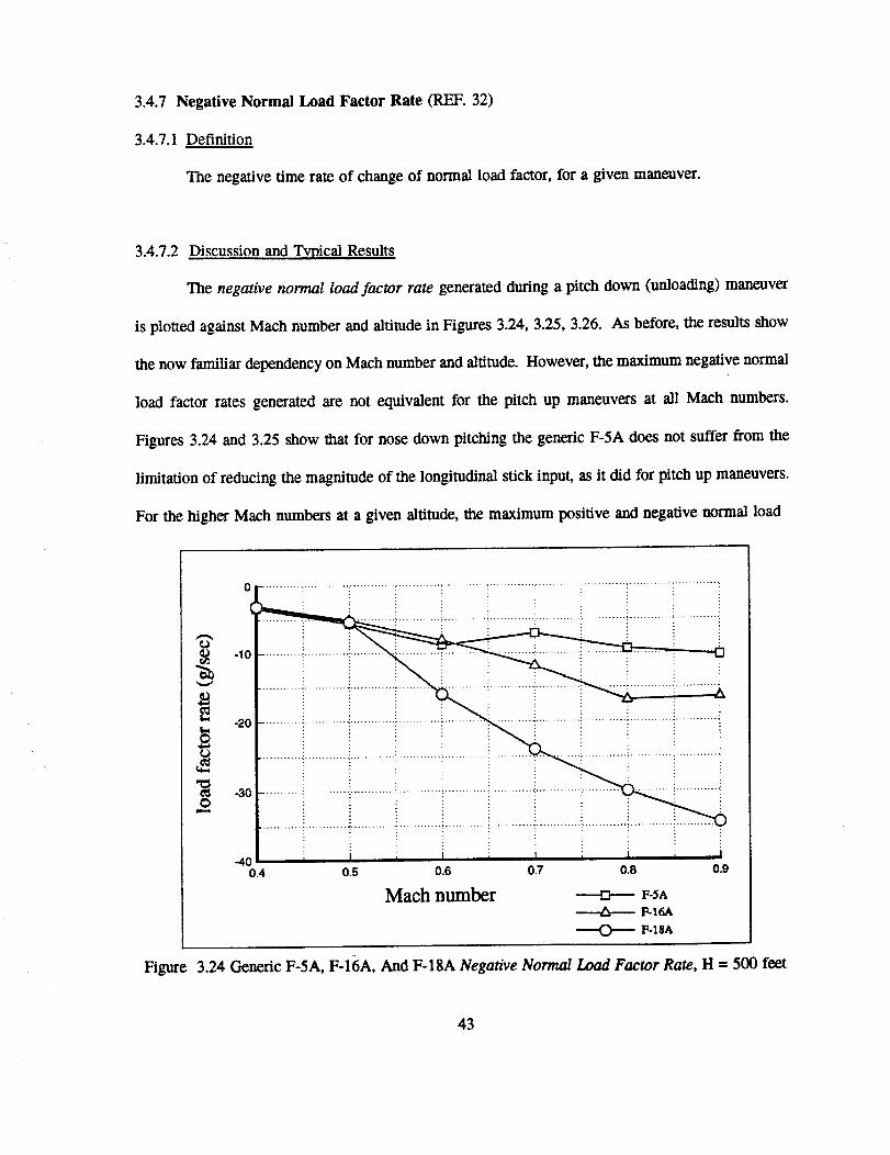
3.4.7 Negative Normal Load Factor Rate (REF. 32)

3.4.7.1 Definition

The negative time rate of change of normal load factor, for a given maneuver.

3.4.7.2 Discussion and Typical Results

The negative normal load factor rate generated during a pitch down (unloading) maneuver

is plotted against Mach number and altitude in Figures 3.24, 3.25, 3.26. As before, the results show

the now familiar dependency on Mach number and altitude. However, the maximum negative normal

load factor rates generated are not equivalent for the pitch up maneuvers at all Mach numbers.

Figures 3.24 and 3.25 show that for nose down pitching the generic F-5A does not suffer from the

limitation of reducing the magnitude of the longitudinal stick input, as it did for pitch up maneuvers.

For the higher Mach numbers at a given altitude, the maximum posiUve and negative normal load

-lC

-20

_o

-40 I I I I i I i I i I0.4 o.s o.8 0.7 o.8

MachnumberF.16A

F-I$A

Figure 3.24 Generic F-5A, F-16A, And F-18A Negative Normal Load Factor Rate, H = 500 feet

43

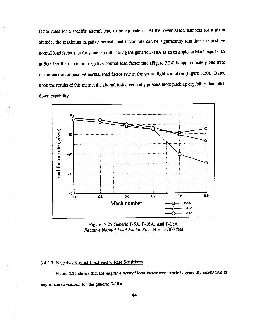
factor rates for a specific aircraft tend to be equivalent. At the lower Mach numbers for a given

altitude, the maximum negative normal load factor rate can be significantly less than the positive

normal load factor rate for some aircraft. Using the generic F-18A as an example, at Math equals 0.5

at 500 feet the maximum negative normal load factor rate (Figure 3.24) is approximately one third

of the maximum positive normal load factor rate at the same flight condition (Figure 3.20). Based

upon the results of this metric, the aircraft tested generally possess more pitch up capability than pitch

down capability.

-I(

-2o

0

-4O0.4

: i

I i I i I I I : •

0.5 0.6 0.7 0.8 0.9

Math number ---o--- F-s.F-16A

F-_SA

Figure 3.25 Generic F-5A, F-16A, And F-18A

Negative Normal Load Factor Rate, H = 15,000 feet

3.4.7.3 Negative Normal Load Factor Rate Sensitivi_

Figure 3.27 shows that the negative normal load factor rate melric is generally insensitive to

any of the deviations for the generic F-18A.

44

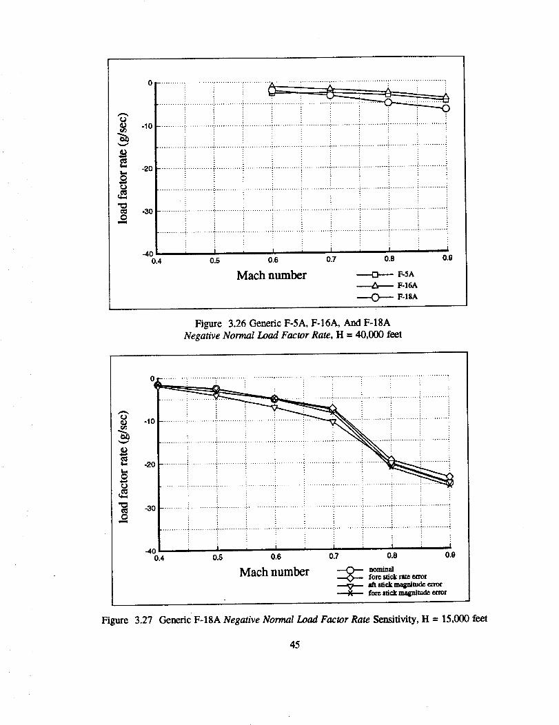
r,j

Otzm=l

-10

-2O

-30

-400,4

........... _............ :............. :............ "K".......... _........................... i............. ; ............ _............. i

i t i I i I i I , I0.5 0.6 0.7 0.8 0.9

Mach number --o-- F SAF-16A

---0---- F-ISA

Figure 3.26 Genetic F-5A, F-16A, And F-18A

Negative Normal Load Factor Rate, H = 40,000 feet

?,

o

Om

0 ............ ;............. :............. ".............. "..................................... ".......................... ' .............

( : •

.o ...........i.............i.............!.............!............::............. i.............!............i............_

: :iillIiiiiiiiiiiiiiiiiiiiilliiiiiiiiiiiiiiiiiiiiliiliiliiiiiii-40

0,4 0.5 0.6 0.7 0.8 0.9

Mach number _ ,o_,fore stick r_ error

aft stick magnitude errorfore midt magnitude error

Figure 3.27 GenericF-18A Negative Normal Load Factor Rate Sensitivity, H = 15,000 feet

45

3.4.7.4 Summary

Since pitch down capability is as tactically important as pitch up capability, the negative

normal load factor rate during a pitch down maneuver was investigated in this report. This metric

is basically analogous to the positive normal load factor rate metric. At the higher Mach numbers,

results for the two metrics are essentially equivalent, while at the lower Mach numbers values for

negative normal load factor rate tend to be lower than the positive normal load factor rate.

Sensitivity results indicate that both of these metrics are insensitive to the deviations applied in this

study. It has been shown in Reference 32 that time histories of normal load factor rate and the

curvature agility metric of Reference 33 are virtually identical when scaled to account for different

units. A derivation and numerical example is supplied in Appendix E.

3.4.8 Average Pitch Rate

3.4.8.1 Definition

Average Pitch Ratet 2 qdt

t 2 - t_

where q is pitch rate, tl is the time at which the pitch-up is executed, and h is the time at

which the pitch-up maneuver is completed. The completion time h is selected at the

discretion of the tester. Usually, h is selected from a common sense point of view for the

particular task which is being performed.

3.4.8.2 Discussion and Typical Results

Referring to Figure 3.3 in Section 3.4.1, for a Mach number of 0.7 and an altitude of 15,000

feet, the generic F-5A has the largest maximum positive pitch rate measured. Based solely upon the

maximum pitch rate criteria of Section 3.4.1, the generic F-5A would be judged to be the most agile

46

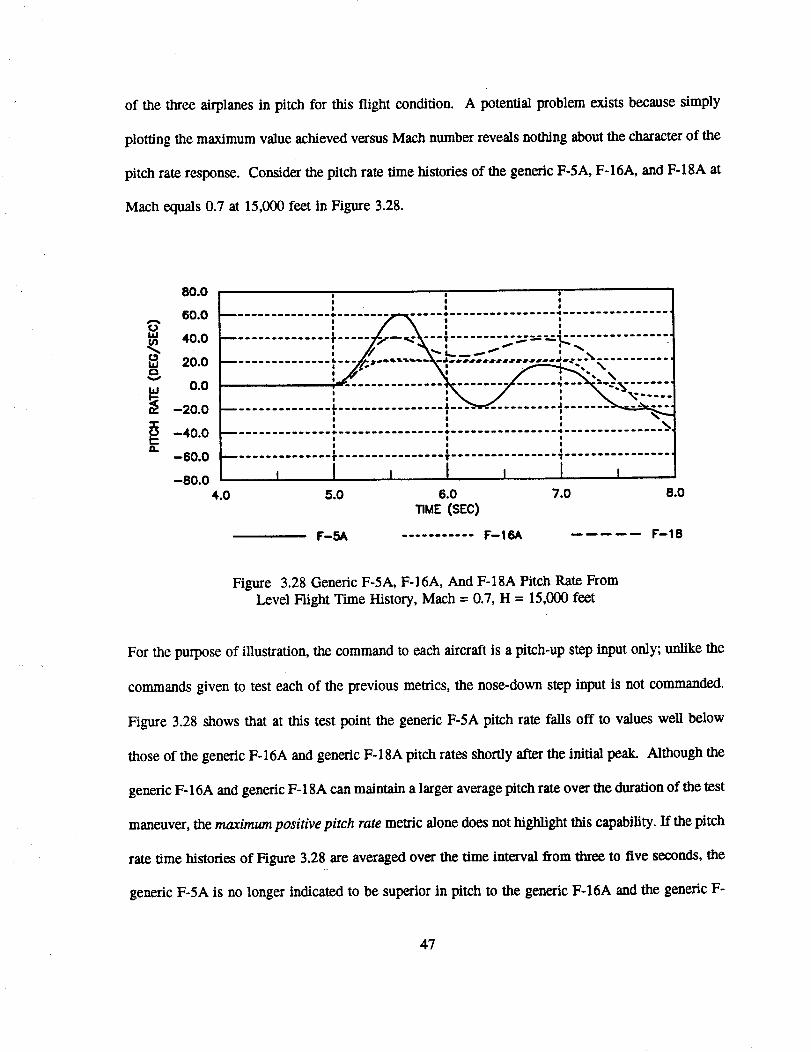
of thethreeairplanes in pitch for this flight condition. A potential problem exists because simply

plotting the maximum value achieved versus Mach number reveals nothing about the character of the

pitch rate response. Consider the pitch rate time histories of the generic F-5A, F-16A, and F-18A at

Mach equals 0.7 at 15,000 feet in Figure 3.28.

80.0I " |

60.0 ................................................................

40.0 ............... r ...... T........ "_':.------_X:- ........0 e ,,,_ e--,, ,0" _.__ ' x

20.0 ............... L... J_,.s,_,,._.T._.-_-at.._ .......e.,d._-.. a eBB _aa_ _ _ ..............# | **

o.o ' -#- '_ _L__..;__._,_ .......

......_,_,_.,_ L................ ' ..........I - !I e I

--40.0 ................................ 4, ..................................o o !

fl. t , i! ! !-60.0 r ................ v................ _.................

-8o.o , I , I , I ,4.0 5.0 6.0 7.0 8.0

TIME (SEC)

F-5A ........... F-16A F-18

Figure 3.28 Generic F-5A, F-16A, And F-18A Pitch Rate FromLevel Hight Time History, Mach = 0.7, H = 15,000 feet

For the purpose of illustration, the command to each aircraft is a pitch-up step input only; unlike the

commands given to test each of the previous metrics, the nose-down step input is not commanded.

Figure 3.28 shows that at this test point the generic F-5A pitch rate falls off to values well below

those of the generic F-16A and generic F-18A pitch rates shortly after the initial peak. Although the

generic F-16A and generic F-18A can maintain a larger average pitch rate over the duration of the test

maneuver, the maximum positive pitch rate metric alone does not highlight this capability. If the pitch

rate time histories of Figure 3.28 are averaged over the time interval from three to five seconds, the

generic F-5A is no longer indicated to be superior in pitch to the generic F-16A and the generic F-

47

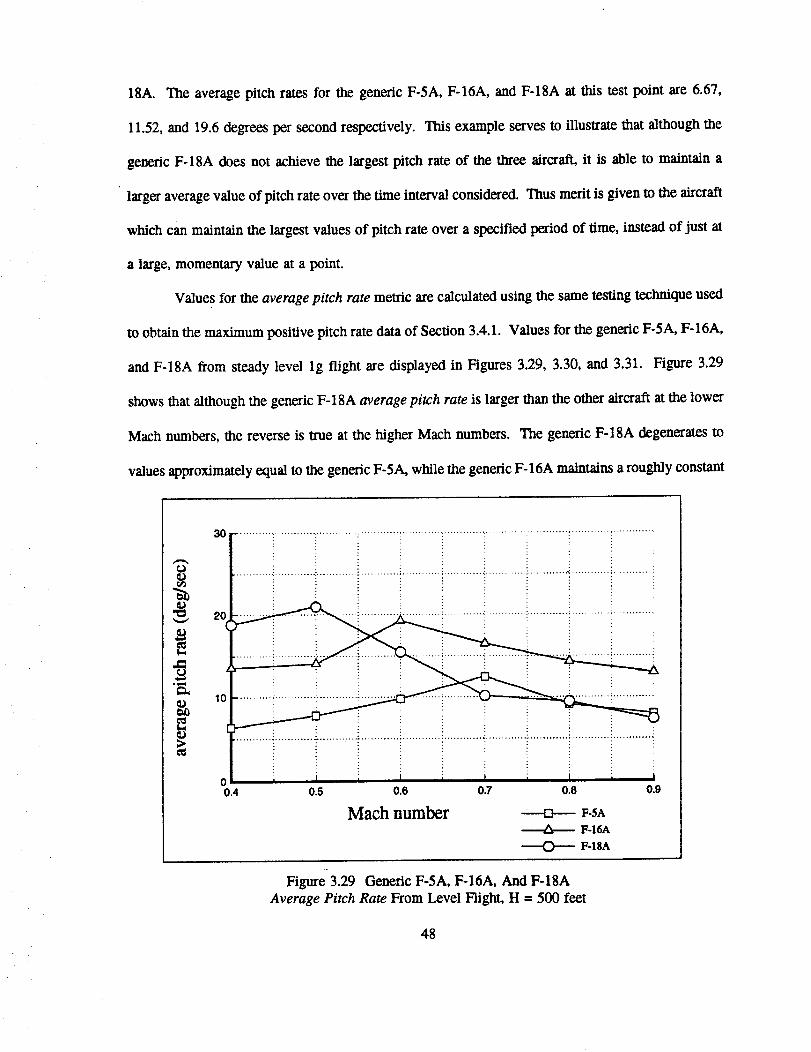
18A. Theaveragepitchratesfor thegenericF-5A,F-16A,andF-18Aat this test point are 6.67,

11.52, and 19.6 degrees per second respectively. This example serves to illustrate that although the

generic F-18A does not achieve the largest pitch rate of the three aircraft, it is able to maintain a

• larger average value of pitch rate over the time interval considered. Thus merit is given to the aircraft

which can maintain the largest values of pitch rate over a specified period of time, instead of just at

a large, momentary value at a point.

Values for the average pitch rate metric are calculated using the same testing technique used

to obtain the maximum positive pitch rate data of Section 3.4.1. Values for the generic F-SA, F-16A,

and F-18A from steady level lg flight are displayed in Figures 3.29, 3.30, and 3.31. Figure 3.29

shoves that although the generic F-18A average pitch rate is larger than the other aircraft at the lower

Mach numbers, the reverse is true at the higher Mach numbers. The generic F-18A degenerates to

values approximately equal to the generic F-5A, while the generic F-16A maintains a roughly constant

i...........i............i.............i............i............i............i.............i............i............i............i

0 I I I t I I t I I I0.4 0.5 0,6 0,7 0.8 0.9

Math number _ F-SAF-16A

F4SA

Figure 3.29 Genetic F-5A, F-16A, And F-18AAverage Pitch Rate From Level Flight, H = 500 feet

48

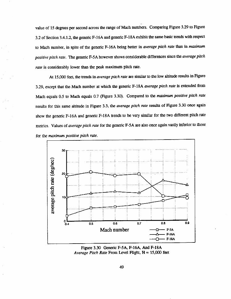
valueof 15degreespersecond across the range of Mach numbers. Comparing Figure 3.29 to Figure

3.2 of Section 3.4.1.2, the generic F-16A and generic F-18A exhibit the same basic trends with respect

to Mach number, in spite of the generic F-16A being better in average pitch rate than in maximum

positive pitch rate. The generic F-5A however shows considerable differences since the average pitch

rate is considerably lower than the peak maximum pitch rate.

At 15,000 feet, the trends in average pitch rate are similar to the low altitude results in Figure

3.29, except that the Mach number at which the generic F-18A average pitch rate is extended from

Mach equals 0.5 to Mach equals 0.7 (Figure 3.30). Compared to the max/mum positive pitch rate

results for this same altitude in Figure 3.3, the average pitch rate results of Figure 3.30 once again

show the generic F-16A and generic F-18A trends to be very similar for the two different pitch rate

metrics. Values of average pitch rate for the generic F-5A are also once again vastly inferior to those

for the maximum positive pitch rate.

30 ........... , ........................... -............. _............ ' ............. • ............. •.............. " ......................... :

i

o| _, i i i i i :, i :, i0.4 0.5 0.6 0.7 0.8 0.9

Mach number ---m--- r-s^F-laA

F-ISA

Figure 3.30 Generic F-5A, F-16A, And F-18A

Average Pitch Rate From Level Flight, H = 15,000 feet

49

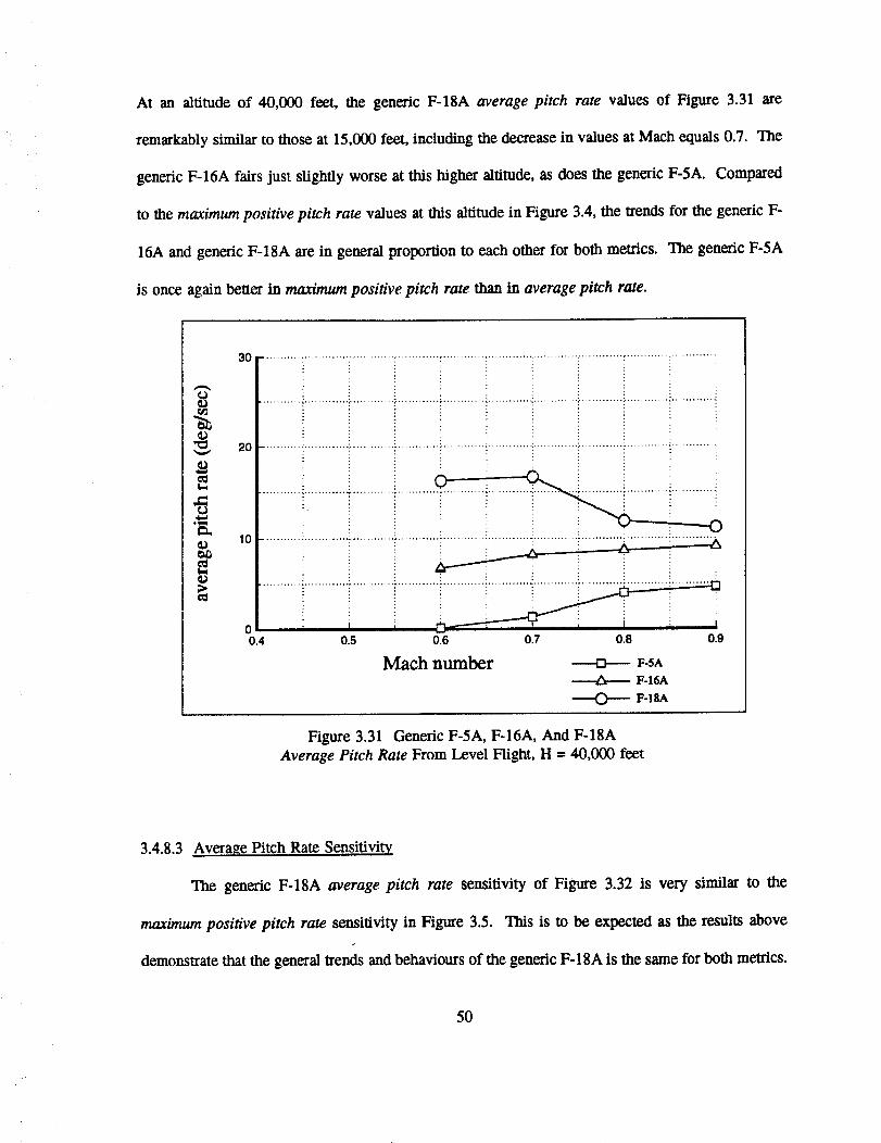
At an altitude of 40,000 feet, the generic F-18A average pitch rate values of Figure 3.31 are

remarkably similar to those at 15,000 feet, including the decrease in values at Math equals 0.7. The

generic F-16A fairs just slightly worse at this higher all_tude, as does the generic F-5A. Compared

to the maximum positive pitch rate values at this altitude in Figure 3.4, the trends for the generic F-

16A and generic F-18A are in general proportion to each other for both metrics. The generic F-5A

is once again better in max/mum positive pitch rate than in average pitch rate.

O

_D

30 ........... • ............. -............. • ............ , ............ • ............. - ............. •............. t ............ . .............

2O

10

00.4

................................................................. :............ ! ............. : ............ i: _ : --A.

.......... _............ .7............ - ............ ; ............ _............ ".-............. :"......................... "........

0.5 0.6 0.7 0.8 0.9

Math number --o-- F-SAF-IaA

---0-- F-lS^

Figure 3.31 Generic F-5A, F-16A, And F-18A

Average Pitch Rate From Level Flight, H = 40,000 feet

3.4.8.3 Average Pitch Rate Sensitivity

The generic F-18A average pitch rate sensitivity of Figure 3.32 is very similar to the

maximum positive pitch rate sensitivity in Figure 3.5. This is to be expected as the results above

demonstrate that the general trends and behaviours of the generic F-18A is the same for both metrics.

50

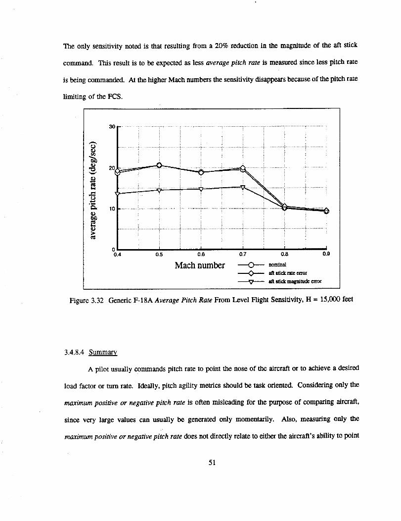
Theonly sensitivity noted is that resulting from a 20% reduction in the magnitude of the aft stick

command. This result is to be expected as less average pitch rate is measured since less pitch rate

is being commanded. At the higher Mach numbers the sensitivity disappears because of the pitch rate

limiting of the FCS.

30 ........... • .............. . ............ • ........................ , ............. . ............. ............... • ........... • ...........

ga,

2O

10

0 i I i 1 i0.4 0.5 0.6

Mach number

I i I i I0.7 0.8 O.O

nominal0 _t =tickrm =for

aft _ck magnitude error

Figure 3.32 Generic F-18A Average Pitch Rate From Level Flight Sensitivity, H = 15,000 feet

3.4.8.4 Summary

A pilot usually commands pitch rate to point the nose of the aircraft or to achieve a desired

load factor or turn rate. Ideally, pitch agility melrics should be task oriented. Considering only the

maximum positive or negative pitch rate is often misleading for the purpose of comparing aircraft,

since very large values can usually be generated only momentarily. Also, measuring only the

maximum positive or negative pitch rate does not directly relate to either the aircraft's ability to point

51

thenoseor to achievea desired load factor.

pitch rate which is desirable to measure.

From this task oriented point of view, it is the average

3.5 SUMMARY

The time to pitch to maximum load factor and the time to unload to zero normal load factor

metrics contain inherent limitations for comparison among dissimilar aircraft or even among various

flight conditions for the same aircraft because the maximum normal load factors can be very different

at the same flight condition. For example, consider two dissimilar aircraft. The first (aircraft A) with

a 5g maximum normal load factor capability at a certain flight condition, and the second (aircraft B)

with a 9g capability at that same flight condition. If both are equally agile in terms of positive normal

load factor rate, then aircraft A will have a shorter time to achieve it's maximum normal load factor

since the maximum normal load factor is a lower value. Likewise, results of the generic F-18A

simulation at an altitude of 15,000 feet demonstrate the same t/me to pitch to maximum normal load

factor at Mach equals 0.6 and at Mach equals 0.7. The reason for this apparent anomaly is that at

Mach equals 0.7, the aircraft has both a higher normal load factor rate and a higher value of

maximum normal load factor.

Maximum positive and negative pitch rate is only an indirect measure of the ability of an

aircraft to generate normal accelerations and to unload quickly to zero normal load factor.

Additionally, differences in lift curve slopes are neglected as they would be in measuring the time to

capture angle of attack. Pitch rate is a direct measure of pilot ability to point the nose of the aircraft,

which is a significant capability during within-visual-range engagements. Although limited because

of the "more is better" property of this metric, assessing pitch agility by plotting max/mum positive

and negative pitch rate versus angle of attack also appears to have some merit. Some advantages of

52

thisapproachare:

l°

.

Since the pilot is not required to capture a specific angle of attack ornormal load factor, his inputs are simpler and more repeatable. As

a result aircraft characteristics are highlighted, and the impact of

individual pilot technique is minimized.

A more complete picture of the aircraft's nose pointing ability is

presented than with other metrics.

In summary, the sensitivity analysis indicates that as tested using the generic F-18A, none of

the candidate pitch agility metrics tested are unusually sensitive to deviations from the nominal

sequence of stick input commands. In the nose up direction, positive pitch rate is reduced by

approximately ten degrees per second if four inches of aft stick is applied rather than the maximum

of five. During the pitch down portion of the maneuvers, zero normal load factor is achieved more

quickly when additional forward slick is applied. Except for these two instances, the input deviations

studied here had no significant effect on the values of the metrics. This would appear to indicate that

,at least for the generic F-18A, useful data for the time to maximum normal load factor and maximum

normal load factor rate metrics possess a reasonable tolerance to variations in pilot input These

sensitivities could apply when using other fighter aircraft to obtain data, but naturally with differing

magnitudes of errors. Additionally, when attempting to collect data to measure maximum positive or

negative pitch rate, or the time to achieve zero normal load factor, unique cockpit displays may be

helpful to allow more precise inputs.

The interaction of flying qualtities and pitch agility metrics becomes especially important when

manned simulators and actual flight testing are used instead of the unmanned non real-time simulations

used for these investigations. For coverage of this aspect of pitch agility the reader is encouraged to

consult Reference 34. ..

53

4. LATERAL AGILITY

4.1 BACKGROUND

Lateral agility is concerned primarily with rolling maneuvers, usually at intermediate or high

angles of attack, and elevated normal load factors. The purposes of this chapter is to analyze the

particular aircraft characteristics which enhance/degrade lateral agility; demonstrate methods for testing

and measuring lateral agility using candidate lateral agility metrics; and compare the lateral agility of

the F-5A, F-16A, and F-18A.

Bank angle capture criteria are developed in order to quantify those candidate lateral agility

metrics which require the capture of a target bank angle. The required pilot command inputs, and the

sensitivity of the candidate lateral agility to deviations in the pilot command inputs is presented. The

lateral agility metrics are evaluated using the University of Kansas Flight Research Laboratory's

generic F-5A and generic F-18A aircraft simulations (Appendix B). All roll angles discussed in this

chapter are in the wind axis coordinate system (Appendix C).

4.2 CANDIDATE LATERAL AGILITY METRICS

In recent years agility researchers have proposed numerous metrics to quantify the lateral

agility of fighter aircraft. The proposed melrics include:

1)

2)

3)

4)

time through 90 ° roll angle (Ta_9o)

90 ° roll angle capture (TRcg0)

180 ° roll angle capture (TRclso)

torsional agility

54

/

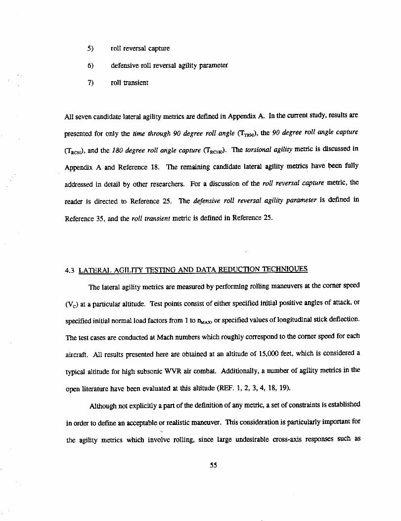
5)

6)

7)

roll reversal capture

defensive roll reversal agility parameter

roll transient

All seven candidate lateral agility metrics are defined in Appendix A. In the current study, results are

presented for only the t/me through 90 degree roll angle (Frv.9o), the 90 degree roll angle capture

(Ttcg0), and the 180 degree roll angle capture (TRcaso). The torsional agility metric is discussed in

Appendix A and Reference 18. The remaining candidate lateral agility metrics have been fully

addressed in detail by other researchers. For a discussion of the roll reversal capture metric, the

reader is directed to Reference 25. The defensive roll reversal agility parameter is defined in

Reference 35, and the roll transient metric is defined in Reference 25.

4.3 LATERAL AGILITY TESTING AND DATA REDUCTION TECHNIQUES

The lateral agility metrics are measured by performing rolling maneuvers at the comer speed

(Vc) at a particular altitude. Test points consist of either specified initial positive angles of attack, or

specified initial normal load factors from 1 to nMAX,or specified values of longitudinal stick deflection.

The test cases are conducted at Mach numbers which roughly correspond to the comer speed for each

aircraft. All results presented here are obtained at an altitude of 15,000 feet, which is considered a

typical altitude for high subsonic WVR air combat. Additionally, a number of agility metrics in the

open literature have been evaluated at this altitude (REF. 1, 2, 3, 4, 18, 19).

Although not explicitly a part of the definition of any metric, a set of constraints is established

in order to define an acceptable or realistic maneuver. This consideration is particularly important for

the agility metrics which involve rolling, since large undesirable cross-axis responses such as

55

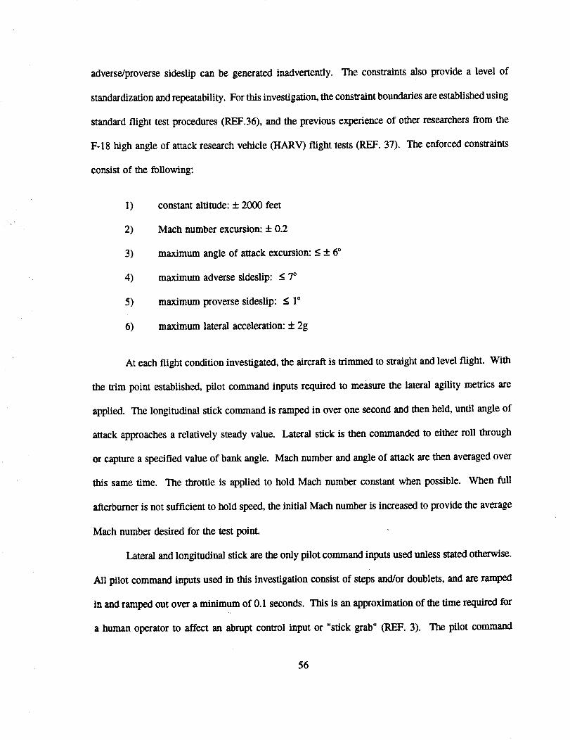
adverse/proversesideslip can be generated inadvertently. The constraints also provide a level of

standardization and repeatability. For this investigation, the constraint boundaries are established using

standard flight test procedures (REF.36), and the previous experience of other researchers from the

F-18 high angle of attack research vehicle (HARV) flight tests (REF. 37). The enforced constraints

consist of the following:

1)

2)

3)

4)

5)

6)

constant altitude: + 2000 feet

Mach number excursion: _+0.2

maximum angle of attack excursion: --. + 6°

maximum adverse sideslip: _<7 °

maximum proverse sideslip: < 1°

maximum lateral acceleration: + 2g

At each flight condition investigated, the aircraft is trimmed to straight and level flight. With

the trim point established, pilot command inputs required to measure the lateral agility metrics are

applied. The longitudinal stick command is ramped in over one second and then held, until angle of

attack approaches a relatively steady value. Lateral stick is then commanded to either roll through

or capture a specified value of bank angle. Mach number and angle of attack are then averaged over

this same time. The throttle is applied to hold Mach number constant when possible. When full

afterburner is not sufficient to hold speed, the initial Mach number is increased to provide the average

Mach number desired for the test point.

Lateral and longitudinal stick are the only pilot command inputs used unless stated otherwise.

All pilot command inputs used in this investigation consist of steps and/or doublets, and are ramped

in and ramped out over a minimum of 0.1 seconds. This is an approximation of the time required for

a human operator to affect an abrupt control input or "stick grab" (REF. 3). The pilot command

56

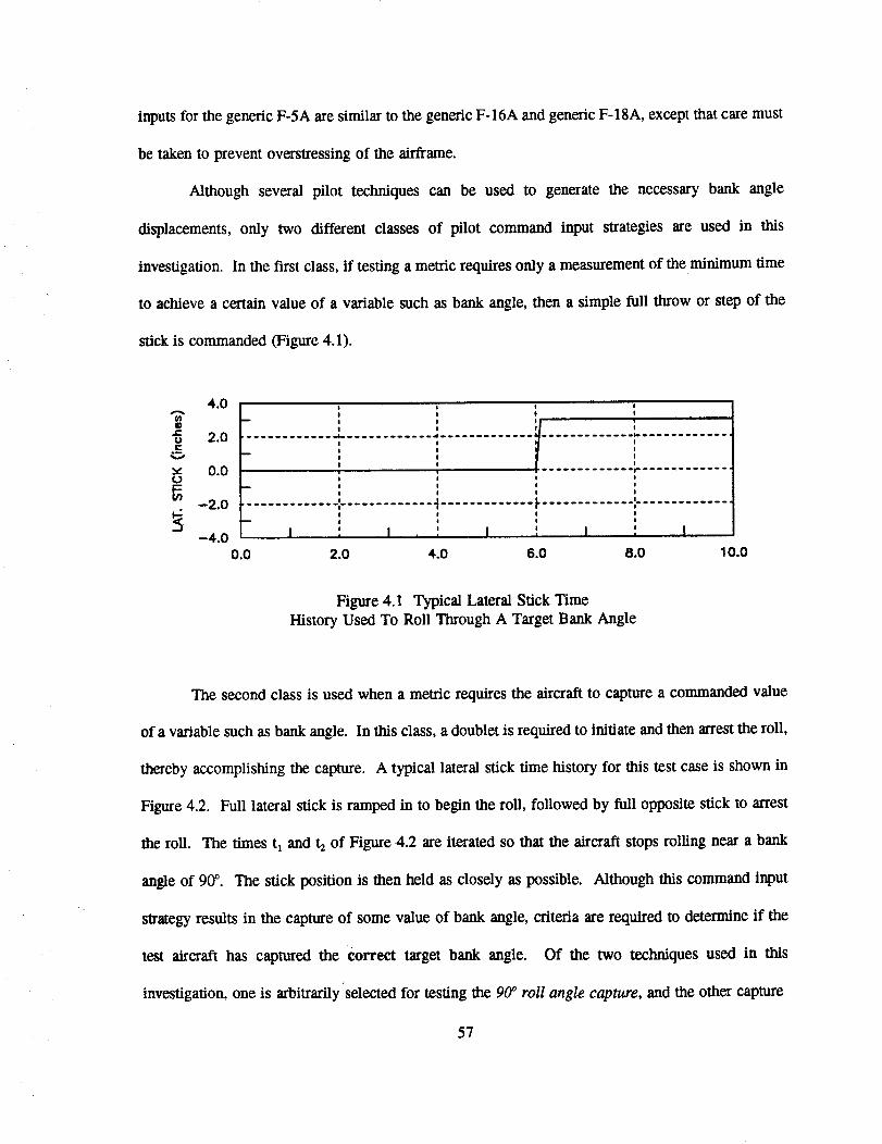
inputs for the generic F-5A are similar to the generic F-16A and generic F-18A, except that care must

be taken to prevent overstressing of the airframe.

Although several pilot techniques can be used to generate the necessary bank angle

displacements, only two different classes of pilot command input strategies are used in this

investigation. In the first class, if testing a metric requires only a measurement of the minimum time

to achieve a certain value of a variable such as bank angle, then a simple full throw or step of the

stick is commanded (Figure 4.1).

%-Ot-Ut-

.mv

V

t_

4.0

2.0

0.0

-2.0

-4.00.0

I

, ',

, , , ;! . I............. ,............. _............. F............. ,"............ "! ! ! I

I I e I

! II , I • , I , I , I

2.0 4.0 6.0 8.0 10.0

Figure 4.1 Typical Lateral Stick Time

History Used To Roll Through A Target Bank Angle

The second class is used when a metric requires the aircraft to capture a commanded value

of a variable such as bank angle. In this class, a doublet is required to initiate and then arrest the roll,

thereby accomplishing the capture. A typical lateral stick time history for this test case is shown in

Figure 4.2. Full lateral stick is ramped in to begin the roll, followed by full opposite stick to arrest

the roll. The times tl and t2 of Figure 4.2 are iterated so that the aircraft stops rolling near a bank

angle of 90°. The stick position is then held as closely as possible. Although this command input

strategy results in the capture of some value of bank angle, criteria are required to determine if the

test aircraft has captured the correct target bank angle. Of the two techniques used in this

investigation, one is arbitrarily selected for testing the 90 ° roll angle capture, and the other capture

57

4.0.g.

O

u 2.0e-

v 0.00

g-2.0

-4.0

! i ! !! I ! !

o ! ! It

t ! I i! ! !

m ! I !! ! !

! ! ! !j I ! !! ! a I

!

! I I I_ , , : U ,! ! ! !I , I , , I , I , I

0.0 2.0 4.0 6.0 8.0 10.0

Figure 4.2 Typical Lateral Stick Time

History Used To Capture A Target Bank Angle

technique is used for testing the 180 ° roll angle capture.

4.3.1 Measurement Criteria For The Time Through 900 Roll Angle Metric

For testing the TTR90 melric, after setting up the aircraft trimmed at the desired Mach number

and angle of attack, full lateral stick is ramped in and held for the duration of the maneuver (Figure

4.1). The time through a target value of bank angle is measured from the time of application of lateral

stick, to the crossing of t_,_ = 90 ° (Figure 4.3).

4.3.2 Capture Criteria For The 90 ° Roll Angle Capture Metric

The TRcg0 metric is tested in the same manner as the TTR90 metric, except that opposite

maximum lateral stick is commanded to arrest the roll near the target bank angle (Figure 4.2). The

time to capture is approximated numerically using a normalization algorithm. Reference 18 proposed

a capture algorithm formulated in terms of parameters in the body axes. Reference 28 modified this

algorithm to relate the time to capture in terms of bank angle and roll rate in the wind axes:

58

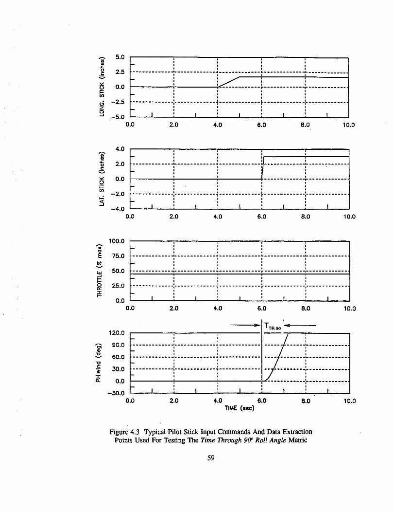
4.0

J;0

._cv

0

co

2.0

0.0

--2.0

--4.00.0

i!

tI m

i

& I

I ' o, I , I , I , I

2.0 4.0 6.0 8.0 10.0

100.0

0

E

k_v

w0n,,

75.0

50.0

25.0

0.00.0

I Ii I

-- i II i

! Ii IiI II i

'lllilIiillll_lilllllllilll_lllililllllll,'llliltliiltlllllllltllllll4

I !! 9

O I

I I I I I , I , I

2.0 4.0 6.0 8.0 10.0

Figure 4.3 Typical Pilot Stick Input Commands And Data Extraction

Points Used For Testing The Time Through 900 Roll Angle Metric

59

90 ° - (q}wt_)m.x (4.1)TRc o-- Tsc+(P,_nd)max

The times are normalized to a bank angle displacement of exactly 90 °. Precise capture of the target

bank angle is not required. Instead, only the capture of a bank angle close to the target angle

(approximately + 10°) is required. Equation 4.1 takes the amount of ¢,_t_ overshoot or undershoot

and computes the time it would have taken to traverse that angle at the maximum rate (Pw._) achieved

during the roll. The time is then added or subtracted from the measured time (TRc), defined as the

time from the application of lateral stick until roll rate reaches zero, to get the normalized time (Figure

4.4).

To see how accurate the normalization procedure is, the time at which the stick deflection was

reversed was varied up to + 0.1 seconds. This created a range of overshoots and undershoots of 90°.

Figure 4.5 shows that despite overshoots and undershoots of more than 10°, consistent TRCg0data can

be predicted.

When using non real-time unmanned simulations, the capture algorithm technique is only

effective for evaluating roll angle capture metrics such as TRcgo and TRcls0 when sideslip angles are

relatively small. Figure 4.6 shows a generic F-18A time history of a 12° angle of attack roll where

capturing the target bank angle is not possible. Kinematic coupling during the roll acceleration and

deceleration generate large sideslip angles, and the rudder actuators are not fast enough to follow the

rudder deflection commands. Although the rudders are riding their rate limits almost continuously

three seconds after the roll is initiated, the transients cannot be eliminated, and the target bank angle

cannot he captured.

60

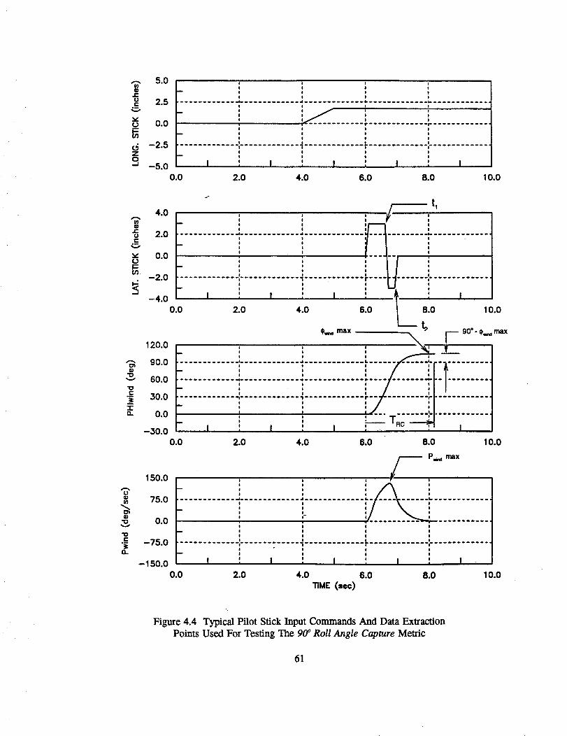
r-

tJ

r"*m

v

,vo

Z

o

(I)

J=

O

.c_V

vo

Lt)

(D

"O

._c

:zn

_n

(I)

'ID

r-

I1.

tl

4.0 : : /--:I ! i rmm_l !

I !iit! I

----:J.H ............ -4-- ............ _ ..................... _ .............I I I ! .

! I I I

I I I

I I I, , --0.0 = , , ;

I I I I =

l l I e

I I !--2.0 .............. ,............. ";..... , ............... ,..............I I ! !- , , I t_ ,

-4.0 I : I : I : : I0.0 2.0 4-.0 6.0 8.0 10.0

--t,*_ max R F 900" _'*'= max

! I !_2o.o _ , , _.' L

'90.0 ............ -:,............. .:............. ,............ :- ...........i I I I =

t_UU--.- ' ' ' 'I I I l

I " I I I

I I I

300 ............ _,............. : ............. ,"'T......... rl.............I I = I, , ,Z ......... LI............., i ' _I

0.0 i I ! t ! I F-' TRc_30.0 i _ I

0.0 2.0 4.0 6.0 8.0 10.0

150.0 F P'_ maxI • !

,I J

75.0 ............ -: ............. -' ............. :-....... '- ...........I J I

$ !

uu-.- ' - '! !

! I

-75.0 '! " I !

I I t I

-150.0 I ', I , I =, I , I

0.0 2.0 4.0 6.0 8.0 10.0TIME (see)

Figure 4.4 Typical Pilot Stick Input Commands And Data Extraction

Points Used For Testing The 90° Roll Angle Capture Metric

61

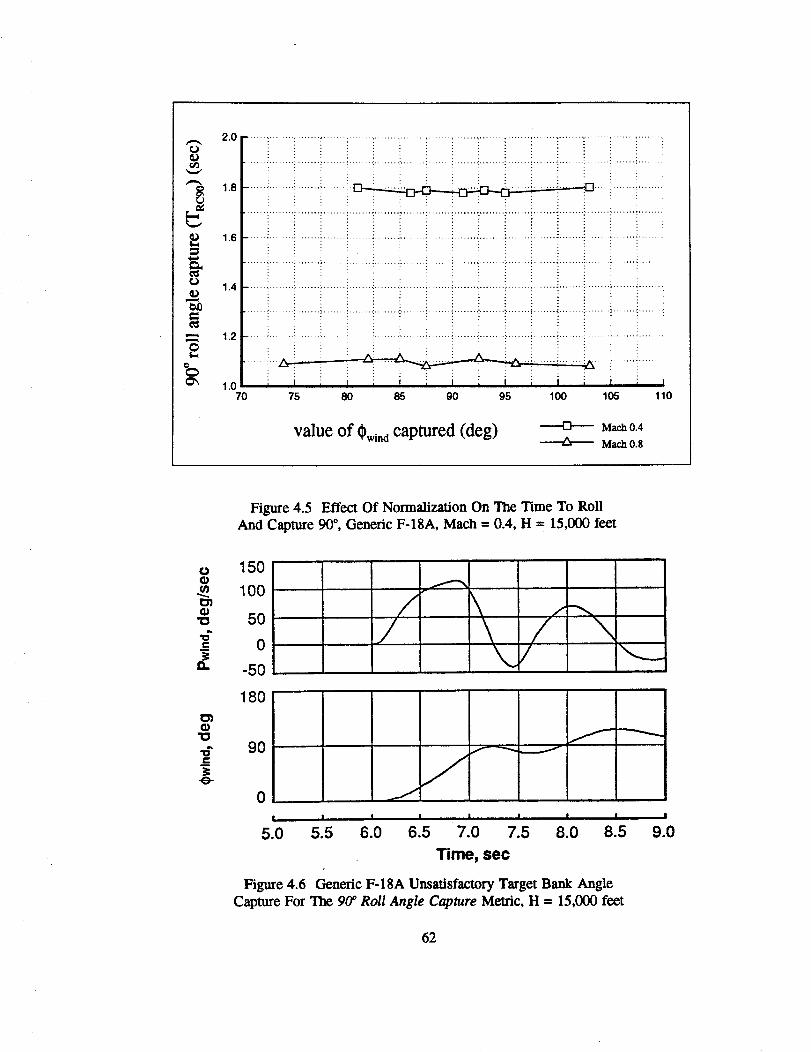
m

2.0 ...... , ........ ......... * ....... . ........ . ........ •....... , ....... , ........ . ........ , ....... . ....... , ........ - ........ • ....... • ........ •

1.8

1.6

1.4

1.2

1.07O

................ _......................... i........................ _........ :........ :-....... _....... --"................................ .:

................ i........ _....... _........ i........................ i ................ i................ ; ................. :........ _........i i. i . . i

! ..... ;

i i i i i i i i i i i i i i i i75 80 85 90 95 100 105 110

value of captured (deg) Mach 0.4

Maeh0.8

Figure 4.5 Effect Of Normalization On The Time To RollAnd Capture 90 °, Generic F-18A, Mach = 0.4, H = 15,000 feet

O

U_ID

'U

e-

fl.

U_

"U

_=

-O-

150

100

5O

0

-50

180

r

9Of_

Jo J

I I I I I I 1 ! I

5.0 5.5 6.0 6.5 7.0 7.5 8.0 8.5 9.0

Time, sec

Figure 4.6 Generic F-18A Unsatisfactory Target Bank Angle

Capture For Tt_e 90 ° Roll Angle Capture Metric, H = 15,000 feet

62

4.3.3 1800 Roll Angle Capture Metric

The TRcls0 metric is tested by first trimming the aircraft to straight and level lg flight. Lateral

stick is then commanded to set the aircraft at the desired -90 ° bank angle. At time equals five

seconds, sufficient longitudinal stick is applied to set the aircraft at the angle of attack specified for

the test point. With the aircraft now banked -90 ° and at the desired angle of attack, the maneuver

commences with the first application of lateral stick, which occurs at time equals seven seconds for

all test cases. Full positive lateral stick is applied and held, then reversed to capture the +90 ° bank

angle (Figure 4.7). Instead of using an algorithm like the one described in Section 4.3.2, bank angle

capture criteria are used to for measuring Tacls0. The criteria are defined as (REF. 7, 38):

1)

2)

maximum overshoot: + 3° after achieving the target bank angle

hold time: 2 seconds after achieving the target bank angle

For a 180 ° roll angle capture maneuver (¢_i= -900, t_t = +90°), the interpretation of the criteria above

is that bank angle must first achieve +900, and then remain there within a six degree band, 87 ° ---

< 93 °, for two full seconds. The band is 3% of the total angular displacement of 180 °. Figure 4.8

shows application of the criteria for a typical successful capture.

A modification of this criteria is required for bank angle responses which decrease

monotonically after achieving the target bank angle. If after achieving the target bank angle, the

response decays monotonically outside the six degree band before two seconds have elapsed, the time

to capture is defined as

t,_c = t._,c, u_s_ + 2 seconds (4.2)

This assumption is justifiable in the case of monotonic bank angle decay because a real-time pilot in

the loop should be able to keep the bank angle within the required six degree band. This is an

63

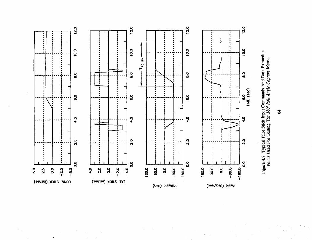
.om.A •o_ o.o -._,

"''I" .... I....

m

I _ I I _ I

o. _. o. _. o

I I

(s0qouO >lOLLS"ONO'I

qr4

ooP

o.00

0

q

qc,,I

q0

u

] TI I

F I I I"" 1 .... r .... I .....I , !! , eJ i i! , O

o 1 Io ! J

i i i0 i 0! I t! II I

0 I! !0 0e !

'

..o. • ._...oo. -I--°-"

I _ i i _, I

o o o. q oI I

(soqouO H:3LLS".LY'I

0

00_

0

qr,,i

q0

:

......... t .... ,"....e ii io i

! ii i -i !

! I oI I ' Il I I

I | lI I1 rI !! I! II 0

: :

! I

: -oI!o

I : I I _ I

q o q q qo d o o o013 _ O_ IX)

"- | T

(80p) pu!_lHd

o

o

o=6

0

qo¢

qo

0

....): : :, , :"" oO I::::1,_, : : ',=_

I _ l

o.

o.0

q0

T

I ! I

q q o. o.0 0 0 OO0 O_"" I

0

(oes/6op) pu!._ d

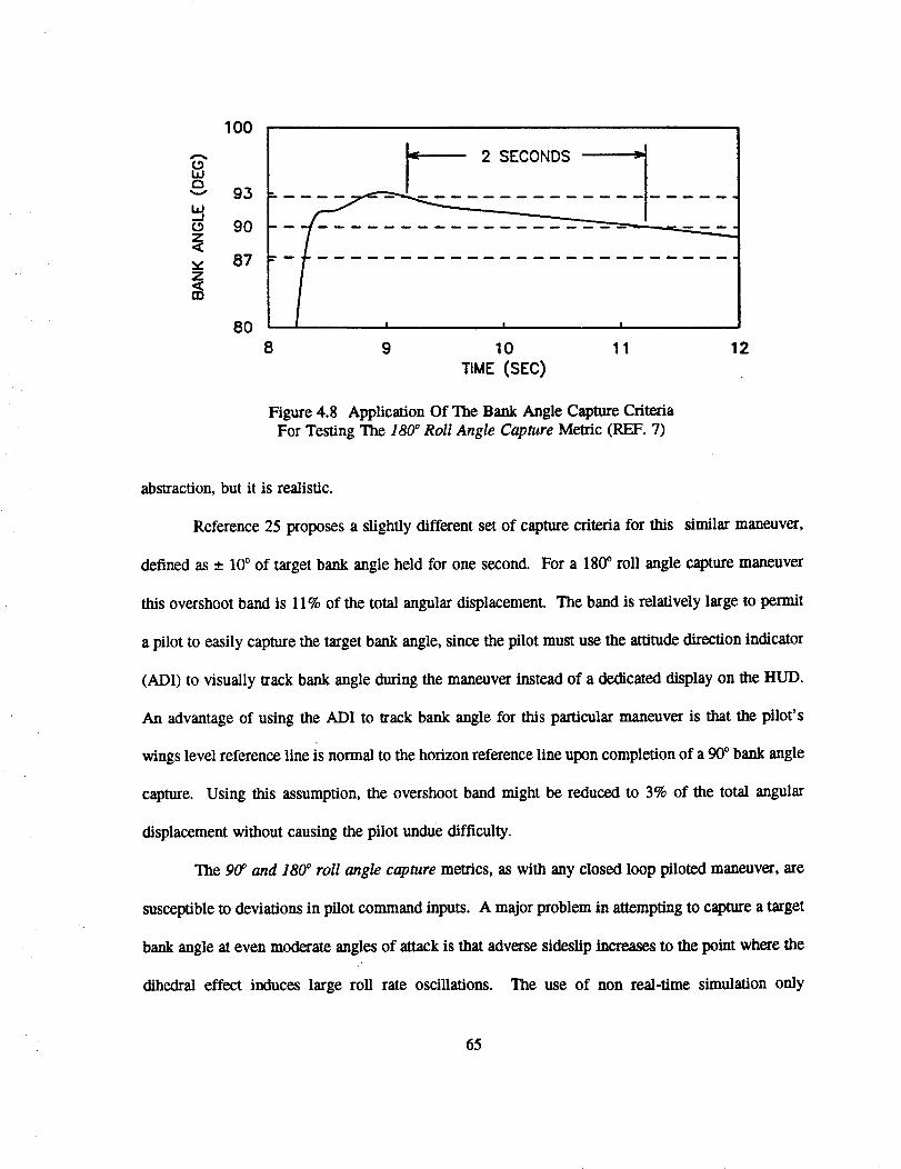
100

2 SECONDS

93

90 -87

80 t , w

8 9 10 11

TIME (SEC)

Figure 4.8 Application Of The Bank Angle Capture CriteriaFor Testing The 180 ° Roll Angle Capture Metric (REF. 7)

12

abstraction, but it is realistic.

Reference 25 proposes a slightly different set of capture criteria for this similar maneuver,

defined as __.10° of target bank angle held for one second. For a 1800 roll angle capture maneuver

this overshoot band is 11% of the total angular displacement. The band is relatively large to permit

a pilot to easily capture the target bank angle, since the pilot must use the attitude direction indicator

(ADI) to visually track bank angle during the maneuver instead of a dedicated display on the HUD.

An advantage of using the ADI to lrack bank angle for this particular maneuver is that the pilot's

wings level reference line is normal to the horizon reference line upon completion of a 90 ° bank angle

capture. Using this assumption, the overshoot band might be reduced to 3% of the total angular

displacement without causing the pilot undue difficulty.

The 90 ° and 180 ° roll angle capture metrics, as with any closed loop piloted maneuver, are

susceptible to deviations in pilot command inputs. A major problem in attempting to capture a target

bank angle at even moderate angles of attack is that adverse sideslip increases to the point where the

dihedral effect induces large roll rate oscillations. The use of non real-time simulation only

65

compounds the problem.

The generic F-18A simulation is used to assess the sensitivity of the lateral agility metrics.

It is important to note timt these sensitivity results are specific to the generic F-18A only, and cannot

be generalized to all fighter aircraft. The intent here is simply to determine in a broad sense how

sensitive the lateral agility metrics can be to pilot inputs, and to demonstrate one way in which an

analysis of this type can be conducted. Since this analysis is simply intended to show typical

behavior, the sensitivity tests are limited to a single altitude of 15,000 feet. The sensitivity of the time

through roll angle metric is not analyzed since the pilot stick input command consists of a single

maximum magnitude step which is held for the duration of the maneuver (Figure 4.1). The nominal

sequence of pilot command inputs are defined here as those inputs which generate the best roll angle

capture performance. If Figure 4.2 represents the nominal pilot command inputs for the roll angle

capture metrics, then the actual pilot command input can deviate from the nominal inputs in five ways

(REF. 3):

1)

2)

3)

4)

5)

Aft stick position relaxed during the roll instead of being held

constant. This deviation was prevalent during F-18A agility flight

testing.

Less than full lateral stick is applied to initiate the roll.

Less than full opposite lateral stick is applied to arrest the roll.

Longitudinal and lateral stick inputs are applied at incorrect rates.

Full opposite lateral stick held too long before arresting the roll.

Deviations two and five are not tested. If less than full lateral stick is applied to initiate the roll, while

the timing of all inputs is the same as the nominal case, as in number two above, the target bank angle

is never achieved. The effect of a deviation like number five above is that the aircraft captures a bank

angle greater than the target bank angle. Figure 4.5 represents the effect of this deviation using the

66

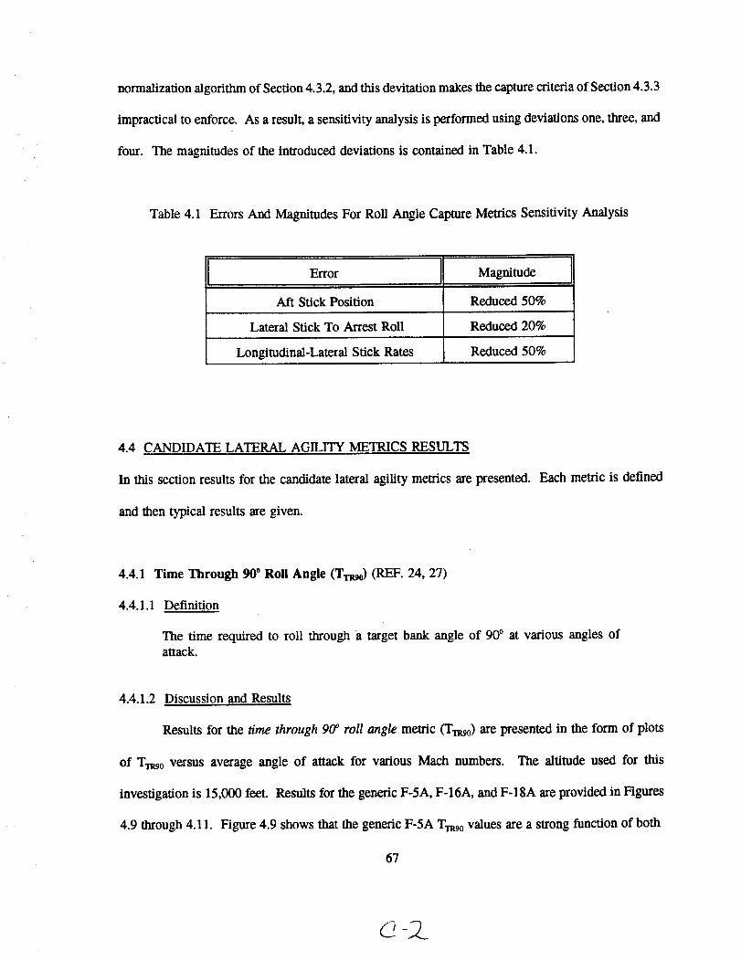
normalizationalgorithmofSection4.3.2,andthisdevitationmakesthecapturecriteriaofSection4.3.3

impracticalto enforce.Asaresult,asensitivityanalysisisperformedusingdeviationsone,three,and

four. Themagnitudesof theintroduceddeviationsis containedin Table4.1.

Table4.1 ErrorsAndMagnitudesForRoll AngleCaptureMetricsSensitivityAnalysis

Error ]

Aft Stick Position Reduced 50%

Lateral Stick To Arrest Roll Reduced 20%

Longitudinal-Lateral Stick Rates Reduced 50%

Magnitude ]

4.4 CANDIDATE LATERAL AGILITY METRICS RESULTS

In this section results for the candidate lateral agility metrics are presented. Each metric is defined

and then typical results are given.

4.4.1 Time Through 90* Roll Angle (Trggo) (REF. 24, 27)

4.4.1.1 .Definition

The time required to roll through a target bank angle of 90 ° at various angles ofattack.

4.4.1.2 Discussion and Results

Results for the t/me through 9& roll angle metric (TTRg0) are presented in the form of plots

of Trv.9o versus average angle of attack for various Mach numbers. The altitude used for this

investigation is 15,000 feet. Results for the generic F-5A, F-16A, and F-18A are provided in Figures

4.9 through 4.11. Figure 4.9 shows that the generic F-5A TTRg0 ValUes are a strong function of both

67

[-

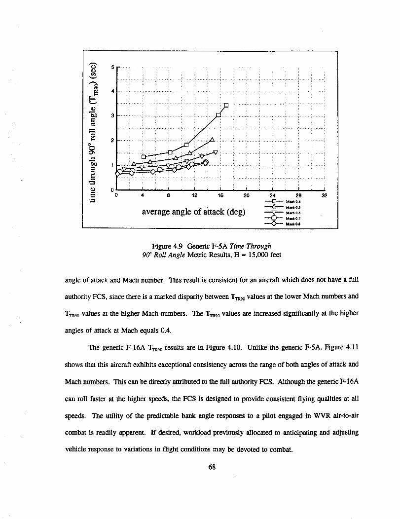
O

_:_ 1

O

ow,,_

: ii i ! i _

................................"........:...........................................................i........i...... :_............

i:iii::iii:::i......'.......................i................i..............!........'........i..............'

i i i i : : : i : i ii _ i _ i T i I i i i i i i , I

4 8 12 18 20 24 28 32M,,m0.4mlcl_ O.5

average angle of attack (deg) _ _'"'_0'.°"

Figure 4.9 Generic F-5A Time Through

900 Roll Angle Metric Results, H - 15,000 feet

angle of attack and Mach number. This result is consistent for an aircraft which does not have a full

authority FCS, since there is a marked disparity between TTRg0 values at the lower Mach numbers and

TTR90 values at the higher Mach numbers. The TTRg0 values are increased significantly at the higher

angles of attack at Mach equals 0.4.

The generic F-16A TTRg0 results are in Figure 4.10. Unlike the generic F-5A, Figure 4.11

shows that this aircraft exhibits exceptional consistency across the range of both angles of attack and

Mach numbers. This can be directly attributed to the full authority FCS. Although the generic F-16A

can roll faster at the higher speeds, the FCS is designed to provide consistent flying qualities at all

speeds. The utility of the predictable bank angle responses to a pilot engaged in WVR air-to-air

combat is readily apparent. If desired, workload previously allocated to anticipating and adjusting

vehicle response to variations in flight conditions may be devoted to combat.

68

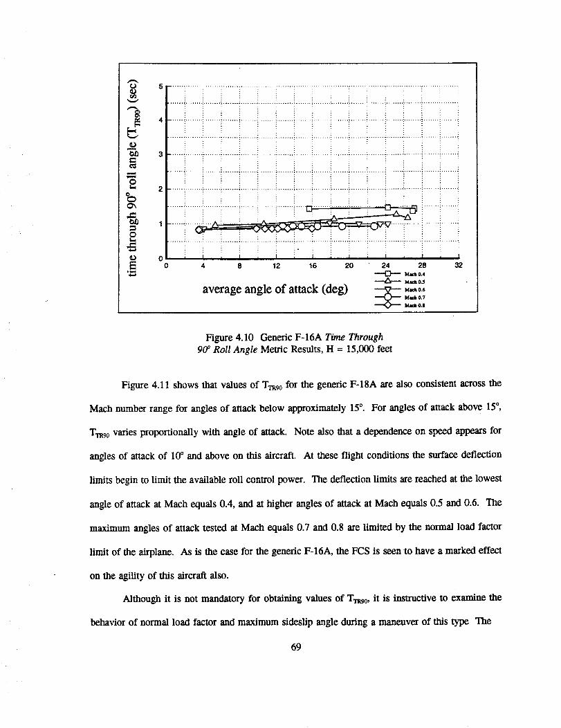
¢J

ID

O

=@

03E

3 .....................................................................................................................................

................ ......... . ............... . ......... . .............. _......................... . ........ . ................. . ...............

i : i

+ ......i_ i......i L .r . i :" .+ _++ + + +....... -+........::........ ;.......i....... _........ :+-.......;....... +........;........_........ ;....... .;........_........ :.......i........_

: !. : i: i : . : : .

o + _ + i + I + i + ,J + i + I + i0 4 8 12 16 20 24 28 32

Math 0.4

Math O.S

average angle of attack (deg) _ ,,.="="='°"o.0'

Figure 4.10 Generic F-16A Time Through90° Roll Angle Metric Results, H = 15,000 feet

Figure 4.11 shows that values of TrRg0 for the generic F-18A are also consistent across the

Mach number range for angles of attack below approximately 15°. For angles of attack above 15°,

TrRg0 varies proportionally with angle of attack. Note also that a dependence on speed appears for

angles of attack of 10° and above on this aircraft. At these flight conditions the surface deflection

limits begin to limit the available roll control power. The deflection limits are reached at the lowest

angle of attack at Mach equals 0.4, and at higher angles of attack at Mach equals 0.5 and 0.6. The

maximum angles of attack tested at Mach equals 0.7 and 0.8 are limited by the normal load factor

limit of the airplane. As is the case for the genetic F-16A, the FCS is seen to have a marked effect

on the agility of this aircraft also.

Although it is not mandatory for obtaining values of T_9o, it is instructive to examine the

behavior of normal load factor and maximum sideslip angle during a maneuver of this type The

69

¢)

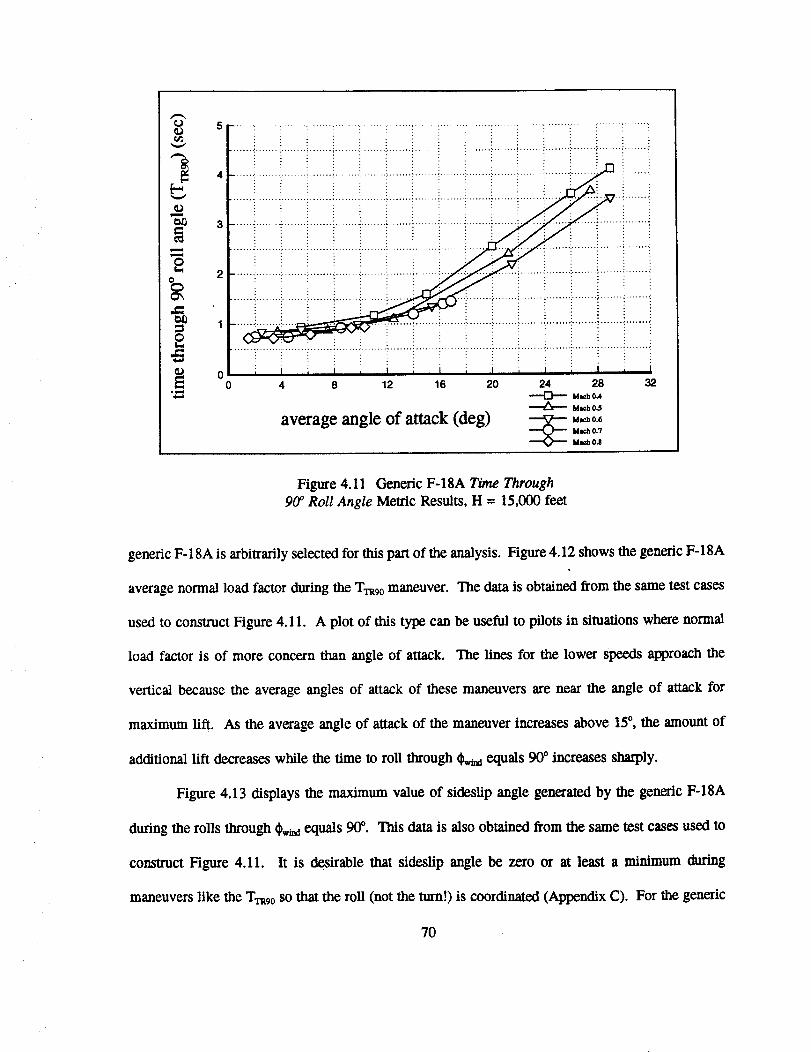
¢)Cx0

2

O

,w,,_

4

3

2

1

......_,........i........i.......',......._,........i.......!.......',........',........U.......i......._,................i.......',.......!0 i I i I i I i I i I i I i I i I

0 4 8 12 16 20 24 28 32Math 0.4

Mae.b 0.5

average angle of attack (deg) _ =="_'_o.,°"°'

Figure 4.11 C-enedc F-18A Time Through

90 ° Roll Angle Metric Results, H = 15,000 feet

generic F- 18A is arbitrarily selected for this part of the analysis. Figure 4.12 shows the generic F-18A

average normal load factor during the TTRg0 maneuver. The data is obtained from the same test cases

used to construct Figure 4.11. A plot of this type can be useful to pilots in situations where normal

load factor is of more concern than angle of attack. The lines for the lower speeds approach the

vertical because the average angles of attack of these maneuvers are near the angle of attack for

maximum lift. As the average angle of attack of the maneuver increases above 15°, the amount of

additional lift decreases while the time to roll through _b,,t_ equals 90 ° increases sharply.

Figure 4.13 displays the maximum value of sideslip angle generated by the generic F-18A

during the rolls through dp,,_ equals 90 °. This data is also obtained from the same test cases used to

construct Figure 4.11. It is desirable that sideslip angle be zero or at least a minimum during

maneuvers like the TzRg0SOthat the roll (not the turn!) is coordinated (Appendix C). For the generic

70

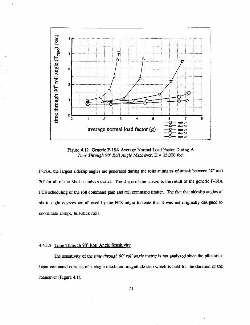
¢D

OD

m

o_

¢)z)

0

°_

iu

4 ........................................ :...... !......................... !........................................................... :

.......i................i.......i.............i.......i......................i..............i........i....i..............i3 ......i........i........i.......i.......i.......i.......i.......i.......i........i.......i.......i........_.......i.......i.......i

iiii12......i........i........i.......i......._........i........i..... i........i........i.......i......i........i........i.......i........ili

0 1 2 3 4 5 6 7 8M_b OA

Mac, b 0.5

average normal load factor (g) _ ...'""o_°"°"

Figure 4.12 Generic F-18A Average Normal Load Factor During A

Time Through 90° Roll Angle Maneuver, H = 15,000 feet

F-18A, the largest sideslip angles are generated during the rolls at angles of altack between 10° and

20 ° for all of the Mach numbers tested. The shape of the curves is the result of the generic F-18A

FCS scheduling of the roll command gain and roll command limiter. The fact that sideslip angles of

six to eight degrees are allowed by the FCS might indicate that it was not originally designed to

coordinate abrupt, full-stick rolls.

4.4.1.3 Time Through 90 ° Roll Angle Sensitivity

The sensitivity of the time through 90 ° roll angle metric is not analyzed since the pilot stick

input command consists of a single maximum magnitude step which is held for the duration of the

maneuver (Figure 4.1).

71

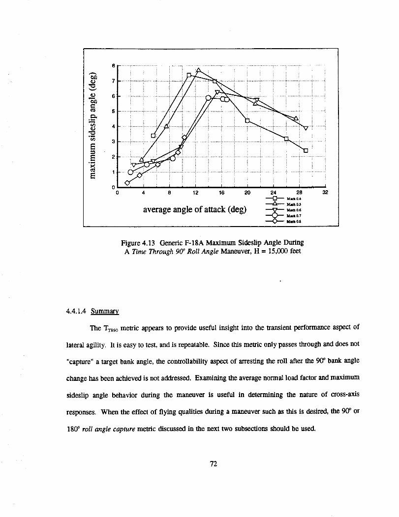
_Dm

°_

¢D

E

E

E

7iiii i6

5

4

3

0 I I I I I I I I I I I I I I t 10 4 8 12 16 20 24 28 32

M_..b 0.4

average angle of attack (deg) _ _"=°'u°"

Figure 4.13 Generic F-18A Maximum Sideslip Angle During

A Time Through 90° Roll Angle Maneuver, H --- 15,000 feet

4.4.1.4 Summary

The TTR90 metric appears to provide useful insight into the transient performance aspect of

lateral agility. It is easy to test, and is repeatable. Since this metric only passes through and does not

"capture" a target bank angle, the controllability aspect of arresting the roll after the 90 ° bank angle

change has been achieved is not addressed. Examining the average normal load factor and maximum

sideslip angle behavior during the maneuver is useful in determining the nature of cross-axis

responses. When the effect of flying qualities during a maneuver such as this is desired, the 90 ° or

180 ° roll angle capture metric discussed in the next two subsections should be used.

72

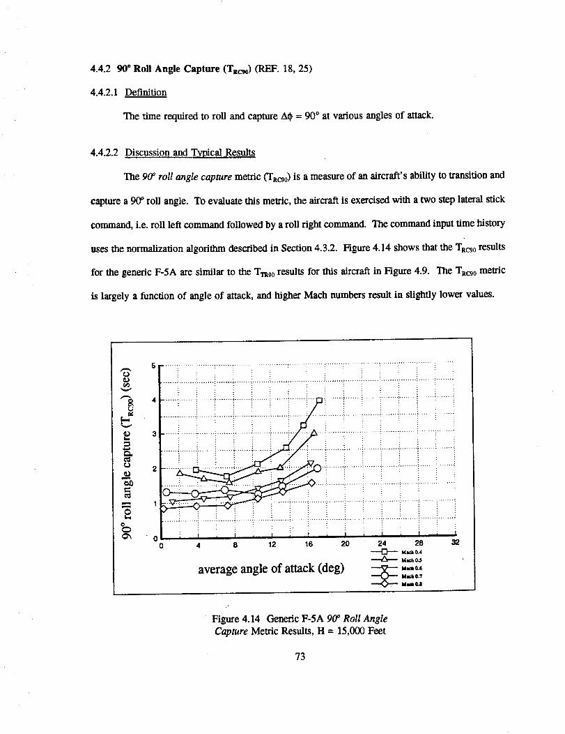
4.4.2 90*Roll Angle Capture (TRoo) (REF. 18, 25)

4.4.2.1 Definition

The time required to roll and capture A(_ = 90 ° at various angles of attack.

4.4.2.2 Discussion and Typical Results

The 90 ° roll angle capture metric (TRcg0) is a measure of an aircraft's ability to transition and

capture a 90 ° roll angle. To evaluate this metric, the aircraft is exercised with a two step lateral stick

command, i.e. roll left command followed by a roll right command. The command input time history

uses the normalization algorithm described in Section 4.3.2. Figure 4.14 shows that the TRcgoresults

for the generic F-5A are similar to the TTRg0 results for this aircraft in Figure 4.9. The TRcg0 metric

is largely a function of angle of attack, and higher Mach numbers result in slightly lower values.

b

e_

O

00

i lili iiii..................................................i................i.............i......i........i...............i................i.......i_......i........!........i.......i.......i........i........i.......i.......i

i 1 I I I I I I i I i I i 1 i I4 8 12 16 20 24 2B 32

Ml_b 0.4

M_ 0.5

average angle of attack (deg) _ .."o"M",,0"

Figure 4.14 Generic F-5A 90 ° Roll Angle

Capture Metric Results, H = 15,000 Feet

73

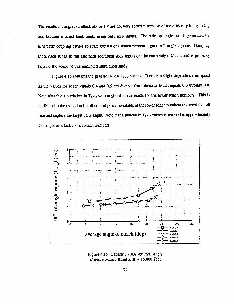
Theresultsfor angles of attack above 10° are not very accurate because of the difficulty in capturing

and holding a target bank angle using only step inputs. The sideslip angle that is generated by

kinematic coupling causes roll rate oscillations which prevent a good roll angle capture. Damping

these oscillations in roll rate with additional stick inputs can be extremely difficult, and is probably

beyond the scope of this unpiloted simulation study.

Figure 4.15 contains the generic F-16A TRcg0values. There is a slight dependency on speed

as the values for Mach equals 0.4 and 0.5 are distinct from those at Mach equals 0.6 through 0.8.

Note also that a variation in TRcgo with angle of attack exists for the lower Mach numbers. This is

attributed to the reduction in roll control power available at the lower Mach numbers to arrest the roll

rate and capture the target bank angle. Note that a plateau in TRcg0values is reached at approximately

23 ° angle of attack for all Mach numbers.

o

t-

ca,

_0

Ox0

0

! : i........ : ........ i.................................................................................. i ................................

i i i :

................................................................................. : ....... i....... - ........ i.........................

......i............................!.......i.......i........i.......i.......i................i.......i........

.......i........_........i.....',.......i........_........i.......i........i........i.......!.......i........i........i.......',.......i I i I i 1 i I i t i I i I i ,I

4 8 12 16 20 24 28 32_0.4

average angle of attack (deg) _ k_'wh°"*,*"

Figure 4.15 Generic F-16A 90_ Roll Angle

Capture Metric Results, H = 15,000 Feet

74

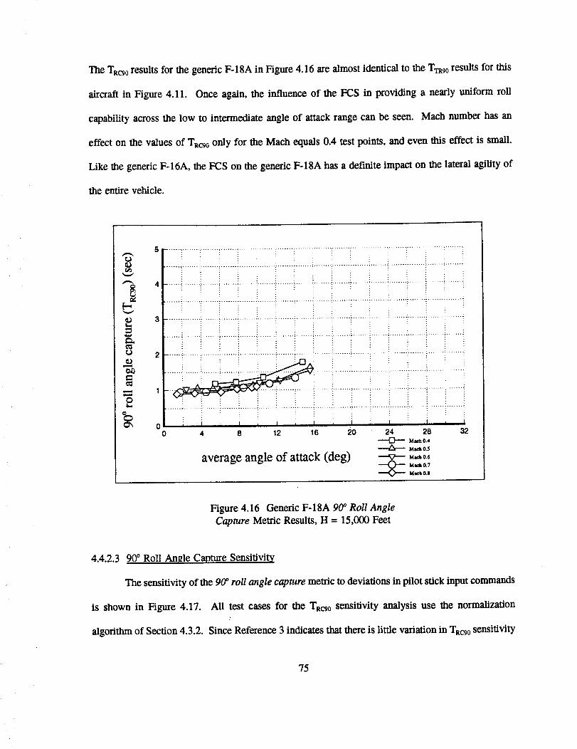
TheTRcg0resultsfor thegenericF-18Ain Figure4.16arealmostidenticalto theTTRg0 results for this

aircraft in Figure 4.11. Once again, the influence of the FCS in providing a nearly uniform roll

capability across the low to intermediate angle of attack range can be seen. Mach number has an

effect on the values of TRcg0 only for the Mach equals 0.4 test points, and even this effect is small.

Like the generic F-16A, the FCS on the generic F-18A has a definite impact on the lateral agility of

the entire vehicle.

[--

@

O'x 00

i

................ i........ :....... _.......................... ! ....... _.................................................. _....... i.........

......"........:........_.......'i......._......._...........i.......i.... i........i......i.......-!........i........i.......!i.......ii i i t i I I I i I i I i I i I

4 8 12 16 20 24 28 32Mlch 0.4

M_ 03

average angle of attack (deg) _ M=o.,Id,.,_ 0.7

Mack 0.8

Figure 4.16 Generic F-18A 90 _ Roll Angle

Capture Metric Results, H = 15,000 Feet

4.4.2.3 90 ° Roll Angle Capture Sensilivity

The sensitivity of the 9& roll angle capture metric to deviations in pilot stick input commands

is shown in Figure 4.17. All test cases for the TRcg0 sensitivity analysis use the normalization

algorithm of Section 4.3.2. Since Reference 3 indicates that there is little variation in Txcgo sensitivity

75

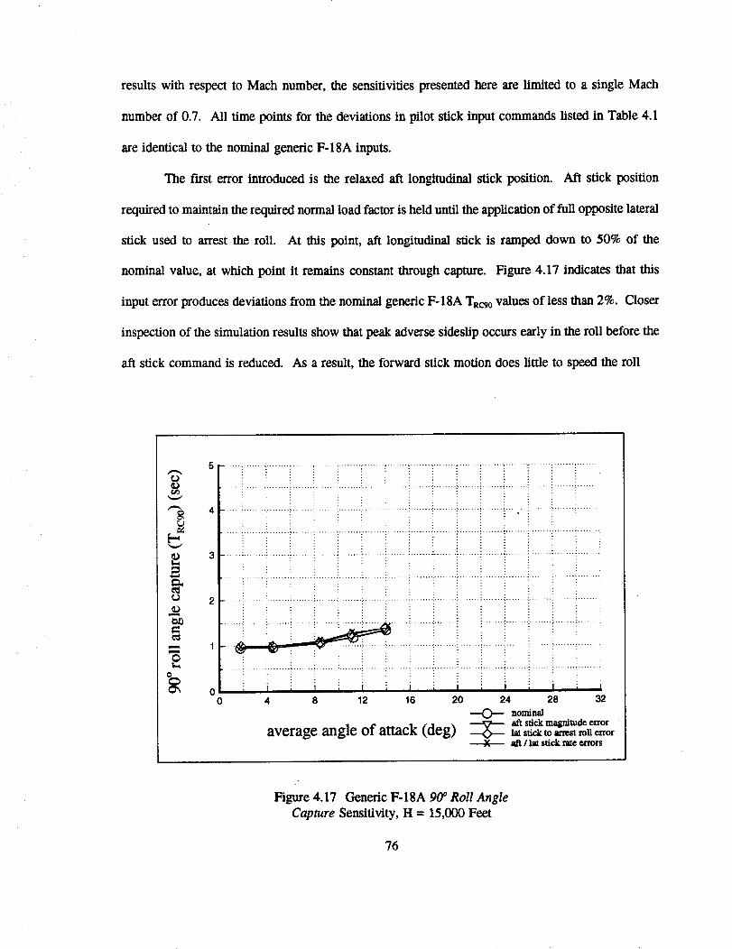
resultswith respectto Machnumber, the sensitivities presented here are limited to a single Mach

number of 0.7. All time points for the deviations in pilot stick input commands listed in Table 4.1

are identical to the nominal generic F-18A inputs.

The first error introduced is the relaxed aft longitudinal stick position. Aft stick position

required to maintain the required normal load factor is held until the application of full opposite lateral

stick used to arrest the roll. At this point, aft longitudinal stick is ramped down to 50% of the

nominal value, at which point it remains constant through capture. Figure 4.17 indicates that this

input error produces deviations from the nominal generic F-18A TRcg0values of less than 2%. Closer

inspection of the simulation results show that peak adverse sideslip occurs early in the roll before the

aft stick command is reduced. As a result, the forward stick motion does little to speed the roll

a

_ 2

1

@

k0

0

.......................................................................................................... ! .........................

: : i i :

..... i........ i........ _....... i........ i i i i !i : i . : : ...., i i I _ i i I i I i J i i i i

4 8 12 16 20 24 28 32

average angle of attack (deg) _ i,,_.tia_"a_tom_'_t_d_t,on"_,,-._ adL_/ I_t stJ¢__ c_ro_

Figure 4.17 Generic F-18A 90* Roll Angle

Capture Sensitivity, H = 15,000 Feet

76

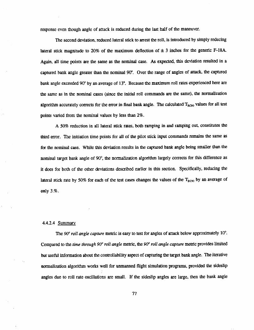
response even though angle of attack is reduced during the last half of the maneuver.

The second deviation, reduced lateral stick to arrest the roll, is introduced by simply reducing

lateral stick magnitude to 20% of the maximum deflection of + 3 inches for the generic F-18A.

Again, all time points are the same as the nominal case. As expected, this deviation resulted in a

captured bank angle greater than the nominal 90 °. Over the range of angles of attack, the captured

bank angle exceeded 90° by an average of 13°. Because the maximum roll rates experienced here are

the same as in the nominal cases (since the initial roll commands are the same), the normalization

algorithm accurately corrects for the error in final bank angle. The calculated TRcgovalues for all test

points varied from the nominal values by less than 2%.

A 50% reduction in all lateral stick rates, both ramping in and ramping out, constitutes the

third error. The initiation time points for all of the pilot stick input commands remains the same as

for the nominal case. While this deviation results in the captured bank angle being smaller than the

nominal target bank angle of 900, the normalization algorithm largely corrects for this difference as

it does for both of the other deviations described earlier in this section. Specifically, reducing the

lateral stick rate by 50% for each of the test cases changes the values of the TRcg0 by an average of

only 3.%.

4.4.2.4 Summary

The 90° roll angle capture metric is easy to test for angles of attack below approximately 10°.

Compared to the time through 90 ° roll angle metric, the 90 ° roll angle capture metric provides limited

but useful information about the controllability aspect of capturing the target bank angle. The iterative

normalization algorithm works well for unmanned flight simulation programs, provided the sideslip

angles due to roll rate oscillations are small. If the sideslip angles are large, then the bank angle

77

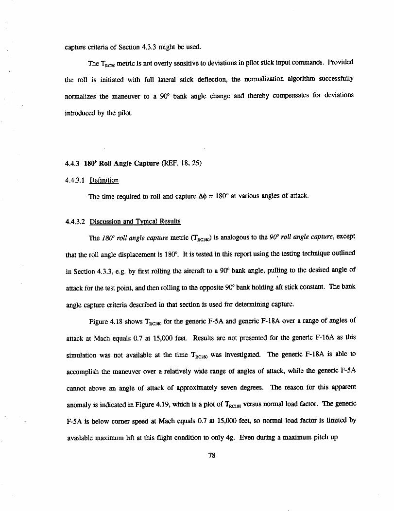
capture criteria of Section 4.3.3 might be used.

The TRcg0metric is not overly sensitive to deviations in pilot stick input commands. Provided

the roll is initiated with full lateral stick deflection, the normalization algorithm successfully

normalizes the maneuver to a 90 ° bank angle change and thereby compensates for deviations

introduced by the pilot.

4.4.3 180 ° Roll Angle Capture (REF. 18, 25)

4.4.3.1 Definition

The time required to roll and capture A_ = 180 ° at various angles of attack.

4.4.3.2 Discussion and Typical Results

The 18& roll angle capture metric (TRcls0) is analogous to the 90_ roll angle capture, except

that the roll angle displacement is 180 °. It is tested in this report using the testing technique outlined

in Section 4.3.3, e.g. by ftrst rolling the aircraft to a 90 ° bank angle, pulling to the desired angle of

attack for the test point, and then rolling to the opposite 90 ° bank holding aft stick constant. The bank

angle capture criteria described in that section is used for determining capture.

Figure 4.18 shows TRcls0 for the generic F-5A and generic F-18A over a range of angles of

attack at Mach equals 0.7 at 15,000 feet. Results are not presented for the generic F-16A as this

simulation was not available at the time TRclso was investigated. The generic F-18A is able to

accomplish the maneuver over a relatively wide range of angles of attack, while the genetic F-5A

cannot above an angle of attack of approximately seven degrees. The reason for this apparent

anomaly is indicated in Figure 4.19, which is a plot of TRC_S0VerSUS normal load factor. The generic

F-5A is below comer speed at Mach equals 0.7 at 15,000 feet, so normal load factor is limited by

available maximum lift at this flight condition to oniy 4g. Even during a maximum pitch up

78

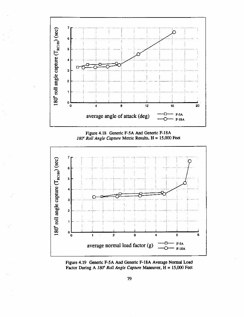
o

j

o

e_0

oO

7

6

5

4

3

2

1

00

.......... • ............. .............. , ............ , ............ • ............. . ............. .............. , ............ , ............. •

iii!

, I i I i I i I i i.4 8 12 16 20

average angle of attack (deg) F-SA

F-18A

Figure 4.18 Generic F-5A And Generic F-18A

180 ° Roll Angle Capture Metric Results, H = 15,000 Feet

o

¢/)

o

=x0

oo

7

6

5

4

3

2

1

00

i I i I i I i _ i I i i1 2 3 4 5 6

average normal load factor (g) F-SA

F-I$A

Figure 4.19 Generic F-5A And Generic F-18A Average Normal Load

Factor During A 18& Roll Angle Capture Maneuver, H = 15,000 Feet

79

maneuverfromwingslevelflight,4.7gis themaximumnormalloadfactorthatthegenericF-5Acan

generate,andeventhenonlymomentarily.Simulationresultsin Reference38clearlydemonstrate

thisbehavior,andtheF-5Aperformancedata in Reference 39 conftrms it. The generic F-18A is not

as severely limited in normal load factor, since it is very near comer speed at this particular flight

condition. However, it is only capable of generating a normal load factor of 6g.

Time histories for the generic F-5A and generic F-18A 7 ° average angle of attack test point

are contained in Figure 4.20. The absence of a throttle ramp input is the only significant difference

in pilot command inputs between the two aircraft for this test point. The bank angle responses in

Figure 4.20 show that the generic F-5A completes the 180 ° transition by achieving the 90 ° bank angle

at about the same time as the generic F-18A, even though the generic F-18A is experiencing high-g

roll rate limiting. The generic F-5A also appears to be much better damped in pitch during this

maneuver, as both normal load factor and angle of attack are only slightly oscillatory. Note that the

generic F-18A angle of attack required to sustain 4g is 18% greater than the same angle of attack

required for the generic F-5A. The corresponding sustained turn rates for both aircraft are 11 degrees

per second. With regard to sideslip angle, the generic F-5A is again well damped, but hits a slightly

greater peak value than the generic F-18A. The maximum lateral acceleration at the pilot's head for

the generic F-5A is 1.1g, and that for the generic F-18A 1.5g.

The complete trajectory of the generic F-18A from trim, to maneuver initiation, to capture for

the 70 average angle of attack test point is displayed in Figure 4.21. Note that Figure 4.21 indicates

the trajectory of the center of mass only, and therefore does not depict angular displacements such as

rolling or yawing. The projection of the trajectory in the XZ plane shows that the generic F-18A

begins losing altitude before the maneuver is initiated. At the initiation point, the sustained turn rate

is 10 degrees per second at a crossrange displacement of 211 feet. The target bank angle is captured

with the aircraft 8,300 feet downrange and 435 feet below the test altitude. The XY projection of the

80

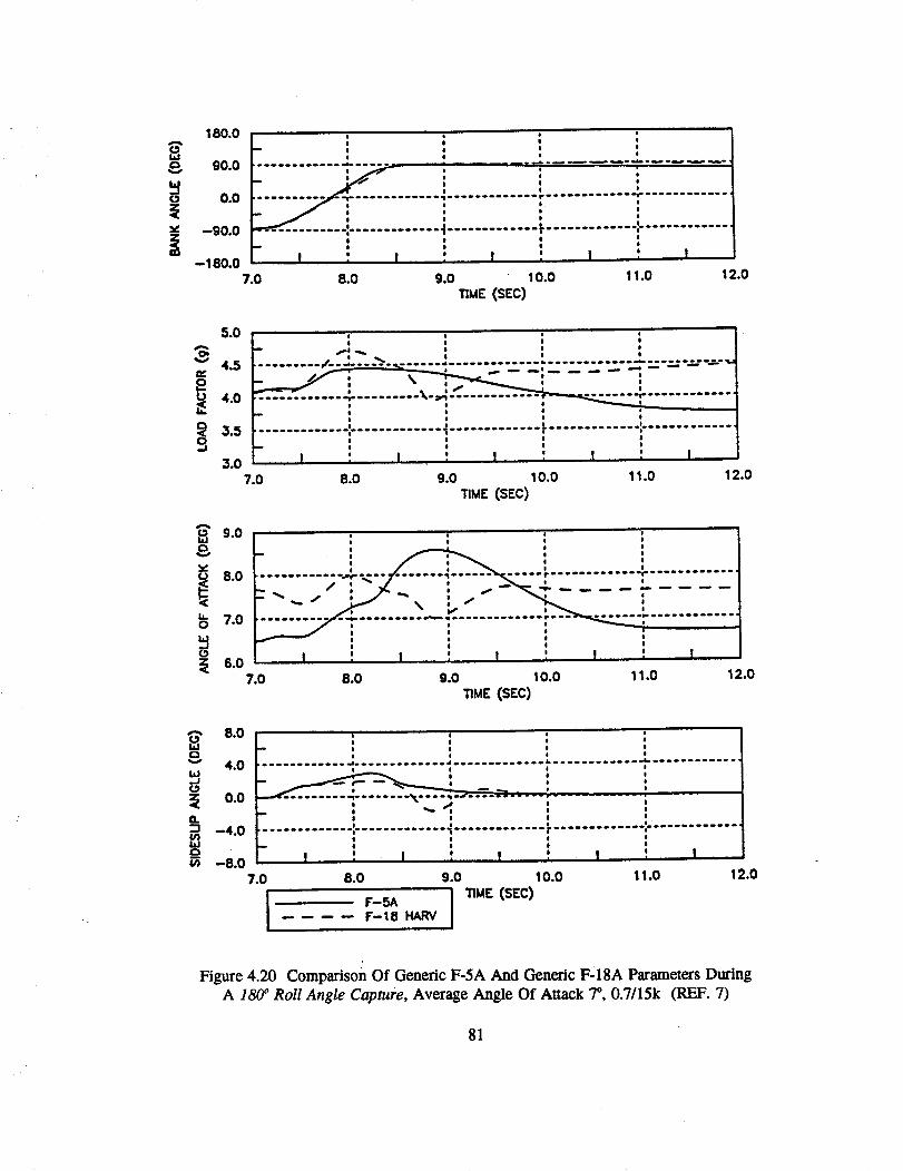
180.0

i 90.00.0

--90.0

- 180.07.0

o *

e e

- " 4s _e o o t

m JL_Sw'r O O e

...................,__---,.,.............t e $. o

e II | eii I i i

•I !" ..... ° ....... ......... °''°O l l I

| l e •

e o e l, I , I , ! , I , I

8.0 9.0 _0.0 1_.0 _2.0_ME(SEC)

i 8.0

O 7.0

6,0

I * I

I I I

I O I *e i i I

l II e I

I ! I I! , I , ! , I , I

7.0 8.0 e.o _0.0 _1.0 12.0TIME (SEC)

V

a.

r/)woIn

8.0

4.0

0.0

-4.0

-8.07.0

I

e

o ie !

,ll.liilliil. _lll II ! lllllt idlillliill ! ill k i i illilitII*_ illiillilil !

' i,,_.."=. ='=._............

e

_ e

I ', I : I , I , I

8.0 9.0 10.0 11.0

F-5AF_18HARV I 'rIME (SEC)

12.0

Figure 4.20 Comparison Of Generic F-SA And Generic F-18A Parameters During

A ]80 ° Roll Angle Capture, Average Angle Of Attack 7°, 0.7/15k (REF. 7)

81

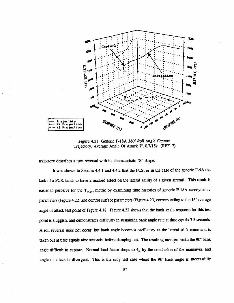
: : : :..!-':'/: .--.: .... : •_'_': ' ;' i.----.! !_' ,,---

" ....!....4.: -

- " .:'" :'_', "E-',-': I+"'-._ _ • : "'-_ ,..P . . ,,. "" I "--..._ : ' i l_,.- . . ,,- • : . . . . ., •

-1¢1"1" , , ' b- , , j. , -L, , L %

'_I : .:-':". '"J_.."_ i '_'-..i

XY Pro j_¢t, ion %Yz Projection I 6-0 '

Figure 4.21 Genetic F-18A 180 ° Roll Angle CaptureTrajectory, Average Angle Of Attack 7°, 0.7/15k (REF. 7)

trajectory describes a turn reversal with its characteristic "S" shape.

It was shown in Section 4.4.1 and 4.4.2 that the FCS, or in the case of the generic F-5A the

lack of a FCS, tends to have a marked effect on the lateral agility of a given aircraft. This result is

easier to perceive for the TRc_o metric by examining time histories of generic F-18A aerodynamic

parameters (Figure 4.22) and control surface parameters (Figure 4.23) corresponding to the 160 average

angle of attack test point of Figure 4.18. Figure 4.22 shows that the bank angle response for this test

point is sluggish, and demonstrates difficulty in sustaining bank angle rate at time equals 7.8 seconds.

A roll reversal does not occur, but bank angle becomes oscillatory as the lateral stick command is

taken out at time equals nine seconds, before damping out. The resulting motions make the 90 ° bank

angle difficult to capture. Normal load factor drops to 4g by the conclusion of the maneuver, and

angle of attack is divergent. This is the only test ease where the 90 ° bank angle is successfully

82

I

eD

|

I....I .... ....r...., | q

e i

, :

-!

O

|

eo

e

!, Io

L/

,......o.,

Itl I!1

o q o q qd o d o o_ | _

I

qw-,

qN

qo

o

w

V

w

q_

q

q

q0

I I '

I e

I i i

I i i

I l I

i i iI I I

"''+I e++'l "'++"

' [i '| 0 I

e e |

e I |

| e e

! e o

o i e

o o el | l

i i

0 I

| e e| 0 0

| 0 !

... +.... _--- +,.. ....I e

i I e

I I

I Ii I

e i

e e i

.oi._+ .p.+--'T'i--_

O I

e i

e|

.... , .... ,..... L!

0

I

e

e o

| e

o |

I . I ' I 'i - - +

o. o. o o. o.

(0) .o_J 0vm

o

o

0

d

o

V

Wop

o.,4"

o.

oo

e... T _.._.--e--

I

0 I

|

o o ,|

... J...l...l....I..I I I

I l

0

O e

O e

I * I * I ' I '

o. o o. o. o o.._ d.+ o .) o

(0:30) )I:DVIIV.t0 ]IONY

o

o

oc_

o

_0G-bJU)

V

LLI2E

o.__D

o.ql-

o.C_l

o.o

I l

e ll l

l I

,e ee i

o |

% .

e e |

0 l !

o I ee I

.. ....L....e....,| I o

I !

e e D| e |

o !

I

I

o

I

: -I

I

t

e

• e +

i

I_1 I_I

q q q _ q

! I

(0]o) _0_ dns3ms

o._r

o

o

c/)V

2Eo._

o.

o.C'4

o.c)

00

me5

G_

I

_E

ce)o0

captured but the angle of attack constraint is violated. Sideslip angle builds to its largest peak

values for this test point, achieving seven degrees both adverse and proverse. This exceeds both

maximum sideslip test constraints. The sideslip angle time history shows that the Dutch Roll mode

has been excited with an equivalent natural frequency of approximately 3.5 radians per second. This

natural frequency meets the applicable Mil-Standard requirement in Reference 40. The equivalent

Dutch Roll damping ratio of approximately 0.28 does not. The resultant sideslip oscillations drive the

roll oscillations at the end of the maneuver, and the capture criteria is not satisfied. The effect of

these oscillations is that the lateral stick command must be reversed at a point where bank angle is

approximately 30° short of the target bank angle. While direct comparisons cannot be made with the

sideslip excursion requirements in full stick rolls in paragraph 4.6.2 of Reference 40, and the roll rate

oscillation requirements of Paragraph 4.5.1.4, both appear to be violated. Although the aircraft can

successfully complete the task of capturing the target bank angle, the total flying qualities seem to be

less than desirable. This result is in agreement with a similar result in Reference 34.

In Figure 4.23, the generic F-18A FCS is seen to use the stabilators, trailing edge flaps, and

ailerons in unison to generate and coordinate the required roll forces. The trailing edge flaps are not

used at all during at this test point, and both stabilators and ailerons are held at their peak values

longer than in the test points at lower normal load factors. Not unexpectedly, all surfaces experience

some rate limiting during the abrupt transient portions of the pilot command inputs. The rudders are

both position limited at their maximum deflection of 30° at time equals 7.8 seconds, and rate limited

thereafter at the maximum rate of 56 degrees per second.

All of the surfaces on the generic F-18A experience rate limiting to some extent while

performing the TRc18omaneuver. Rate limiting occurs not only at the test points at high angles of

attack and elevated normal load factors, but at all of the test points. However, only the rate limiting

of the rudders significantly affect the performance of the maneuver and the value of TRclao. During

84

12.0

,o,8 8.o

0.0

._ -6.0

-12.00.0

I, : : : :- ,, : ,' : :

I I | I I

, , ; , ; ,I I l l l I

I e l I l l

l I I I

O I l 0 l I

I I | I I

I I I $ I I, I , I , I , I , I , I

2.0 4.0 6.0 8.0 10.0 12.0 14.0TIME(SEC)

_Ea

10.0

5.0

0.0

-5.0

-10.00.0

I I

: ,

' 'I e I.

O I I e I

e l

I | I I I I

I O l

I ! I : ,I : I : I : I , !

2.0 4.0 6.0 8.0 10.0 12.0 14.0_ME (SEC)

A

,o,I::1

V

ZO

E

20.0

10.0

0.0

-10.0

-20.00.0

I I l I l

I I I •I I l

I I I _ I I

O I _i!f i I l

I l ! I I

l l I O e

I l I !

• .. .... L.___-- - • __

, , ; , ; ,I , l O $ l l

I t I | I !

I I I l I l

I II J o I V ' Il I I I I l

I I I V i I : I : I : I : I

2.0 4.0 6.0 8.0 10.0 12.0 14.0TIME (SEC)

A

QV

I,iJ

rm::)iY

40.0

20.0

0.0

-20.0

-40.00.0

: : : : :i I l l I $

' ' _ 'I I l I l I

i I l l I l I

I ! I O e I

I _ e ! e I I

O l _ I I

_ , ,O O I I I

I e I l e I !

I' ' ' 'X--F-1 :I I I I

I I | , I II , I , I , I , I , I , I

2.0 4.0 6.0 8.0 10.0 12.0 14.0_ME (SEC)

Figure 4.23 Generic F-18A Control Surface Activity During A 180 °

Roll Angle Capture, Average Angle Of Attack 16°, 0.7/15k (REF. 7)

85

this investigation, this effect only occurs at the 16° average angle of attack test point. Though not

commanded by the pilot, the rudders are used extensively by the FCS of the generic F-18A. Rather

than using the rudder to drive sideslip to zero, the FCS instead tracks lateral acceleration because of

the Ny feedback system used for turn coordination. While this architecture ensures that lateral

accelerations remain within tolerable levels, it does not eliminate all sideslip during uncoordinated

maneuvers, and may not be utilizing all of the roll capability in the airframe. This is probably a result

of lateral agility, i.e. rolling at high angle of attack, not being a stringent requirement during the

design of the F-18A flight control system. It is not a matter of concern when rolling at low normal

load factors, but it is at elevated normal load factors and high angles of attack where roll control

power decreases and adverse yaw can become large.

Although the TRclso metric is normally measured without any rudder inputs from the pilot,

Reference 38 investigated the utility of these inputs to enhance performance of the maneuver. Two

different pilot rudder command input schemes were used. The first scheme tracked sideslip and used

the rudder to generate an opposing yawing moment which reduces the buildup of adverse yaw. The

presumed benefit of this scheme is that the aircraft is able to perform the maneuver in a more

coordinated fashion. The pilot rudder commands for this scheme consist of a series of doublets. The

second scheme used the rudder to generate and maintain a large proverse yawing moment. Provided

that sufficient rudder control power is available, this has the anticipated effect of inhibiting the buildup

of adverse yaw for at least a short time.

Reference 38 concluded that no practical advantage in improving TRcls0 is to be gained from

using pilot rudder command inputs. The pilot rudder command inputs are not pilot friendly, as the

inputs are of short duration and perturb the aircraft sufficiently as to require additional pilot command

input compensation. The only observed benefit of using the rudders in this manner was a reduction

in sideslip angle and lateral accelerations. No significant increase in bank angle rate was achieved

86

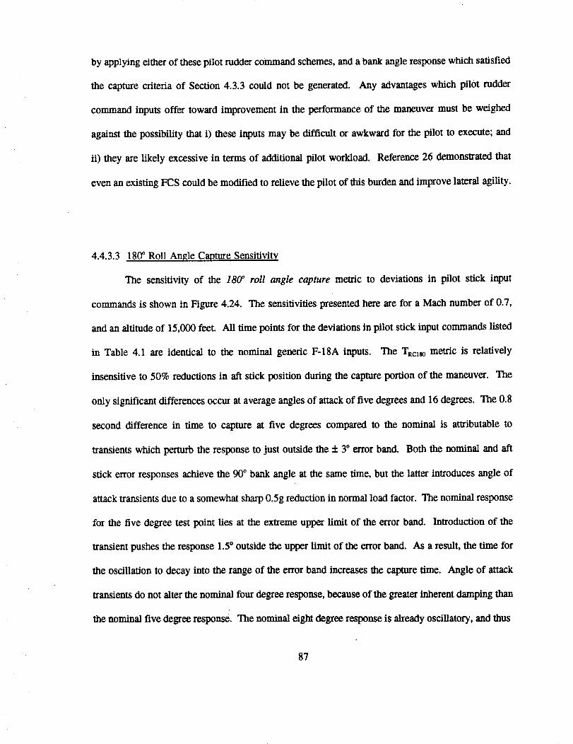
byapplyingeitherofthesepilot ruddercommandschemes,andabankangleresponsewhichsatisfied

the capturecriteriaof Section4.3.3couldnotbe generated.Any advantages which pilot rudder

command inputs offer toward improvement in the performance of the maneuver must be weighed

against the possibility that i) these inputs may be difficult or awkward for the pilot to execute; and

ii) they are likely excessive in terms of additional pilot workload. Reference 26 demonstrated that

even an existing FCS could be modified to relieve the pilot of this burden and improve lateral agility.

4.4.3.3 180° Roll Angle Capture Sensitivity

The sensitivity of the 1800 roll angle capture metric to deviations in pilot stick input

commands is shown in Figure 4.24. The sensitivities presented here are for a Mach number of 0.7,

and an altitude of 15,000 feet. All time points for the deviations in pilot stick input commands listed

in Table 4.1 are identical to the nominal generic F-18A inputs. The TRc_s0 metric is relatively

insensitive to 50% reductions in aft stick position during the capture portion of the maneuver. The

only significant differences occur at average angles of attack of five degrees and 16 degrees. The 0.8

second difference in time to capture at five degrees compared to the nominal is attributable to

transients which perturb the response to just outside the + 3° error band. Both the nominal and aft

stick error responses achieve the 90 ° bank angle at the same time, but the latter introduces angle of

attack transients due to a somewhat sharp 0.5g reduction in normal load factor. The nominal response

for the five degree test point lies at the extreme upper limit of the error band. Introduction of the

transient pushes the response 1.5° outside the upper limit of the error band. As a result, the time for

the oscillation to decay into the range of the error band increases the capture time. Angle of attack

transients do not alter the nominal four degree response, because of the greater inherent damping than

the nominal five degree response. The nominal eight degree response is already oscillatory, and thus

87

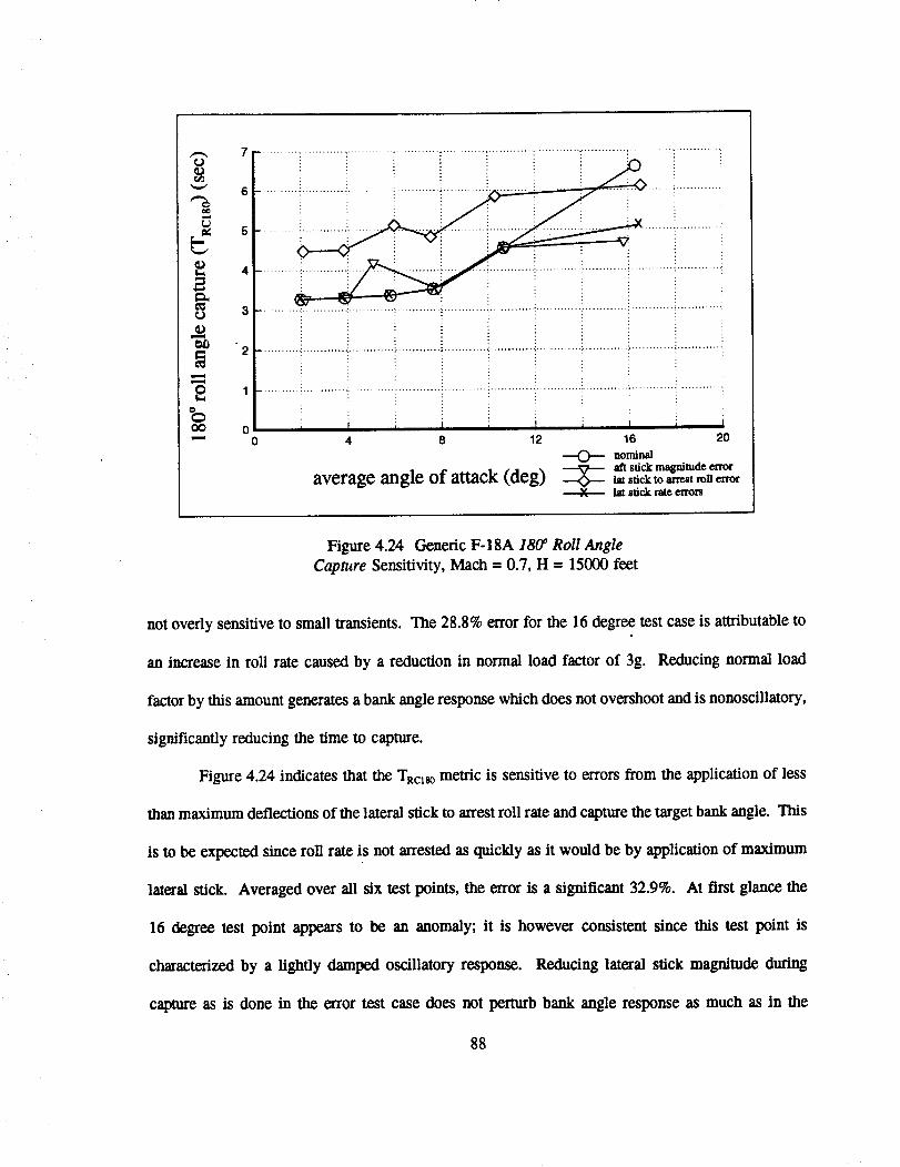
7_

6

5

oo

[--

3eJ

2 1

_ 0_ 0

......................... i ...........................................................................................................

, I , I i I , I i i4 8 12 16 20

--0-- .o_

average angle of attack (deg) _ _ stickm_d_ _rtat stick to arrest roll errorlat stick rate en_ors

Figure 4.24 Generic F-18A 1800 Roll Angle

Capture Sensitivity, Mach = 0.7, H = 15000 feet

not overly sensitive to small transients. The 28.8% error for the 16 degree test case is attributable to

an increase in roll rate caused by a reduction in normal load factor of 3g. Reducing normal load

factor by this mount generates a bank angle response which does not overshoot and is nonoscillatory,

significantly reducing the time to capture.

Figure 4.24 indicates that the TRc180metric is sensitive to errors from the application of less

than maximum deflections of the lateral stick to arrest roll rate and capture the target bank angle. This

is to be expected since roll rate is not arrested as quickly as it would be by application of maximum

lateral stick. Averaged over all six test points, the error is a significant 32.9%. At first glance the

16 degree test point appears to be an anomaly; it is however consistent since this test point is

characterizedby a lightlydamped oscillatoryresponse. Reducing lateralstickmagnitude during

captureas isdone in the errortestcasedoes not perturbbank angleresponseas much as in the

88

nominal case. Although the maximum bank angle achieved is the same in both cases at 16 degrees,

the error response is more damped and requires less time to satisfy the capture criterion. As with the

aft stick error cases, the only seemingly inconsistent trends occur in the higher angle of attack range.

Errors in lateral stick input and output rates do not appreciably affect the test results (Figure

4.24). Averaged over all the test points, this error is only 3.8%. The only standout is the 16 degree

test point, which is in error by 22.7%. It has already been indicated that the nominal 16 degree test

point exhibits light damping and is sensitive to perturbations. The same is Irue when this error is

introduced, as the smaller input and output stick rates produce smaller perturbations than the larger

input and output stick rates of the nominal test case.

The 180 ° roll angle capture metric 16 degree test point is sensitive to errors due to relaxing

aft stick position during capture, ancl reduced lateral stick magnitudes during capture. The generic F-

18A has little difficulty satisfying the capture criterion of Section 4.3.3 at the lower angles of attack,

but has trouble in the 16 test points due to kinematic coupling, reduction in damping in all three axes,

and a heightened sensitivity to perturbations.

4.4.3.4 Summary

Although the 180 ° roll angle capture is similar to the 900 roll angle capture, the longer

duration of the maneuver and the larger bank angle displacement tend to result in a larger buildup of

adverse yaw. This has the effect of making a successful capture increasingly difficult. There appears

to be no specific advantage over the 90 ° roll angle capture metric; it is simply a more challenging task

for the aircraft as explained above. Use of the capture criteria identified a flight condition (test point

for 16 degrees angle of attack) where the generic F-18A could not satisfy the capture criteria. For

other test cases, the capture criteria gave an indication of how easy (or difficult) accomplishing the

89

capture can be. Although more realistic than the normalization algorithm, it is considerably more

demanding and time consuming to use because of the iterative nature of determining the command

sequence that generates the desired results.

When measured using the generic F-18A, the 1800 roll angle capture metric is recognized to

be sensitive to reductions in aft stick magnitude in the higher range of normal load factors.

Comparing the characteristics of the two aircraft, the generic F-5A appears to be better damped in all

three axes, but suffers from being below corner speed at this flight condition. However, the capability

of performing this maneuver over a greater range of angles of attack and near the design limit normal

load factor, may not be tactically significant. Although the normal load factor for the generic F-5A

is limited at this flight condition, it still performs the maneuver quite well. The generic F-18A, on

the other hand, is less damped in all three axes than the generic F-5A, yet is slightly better in

performing the maneuver at all the angles of attack tested.

4.5 .SUMMARY

In summary, the suitability of three candidate lateral agility metrics were tested to determine

for suitability in measuring lateral agility. The maneuvers required to test the lateral agility metrics

are somewhat unique from the standpoint of traditional flight test maneuvers, and could promote pilot

disorientation due to the atypical aircraft attitudes encountered. Disorientation problems can be

partially alleviated through adequate cockpit instrumentation. During this investigation none of the

aircraft exhibited roll reversal or roll ratcheting tendencies, and execution of the maneuvers did not

impose any intolerable linear accelerations upon the pilot.

The time through roll angle metrics, e.g. Tzp.90, as a class are suitable for measuring the

transient performance aspect of lateral agility. The main advantage of this class of metrics is that they

90

measure the same transient performance as the roll angle capture class of melrics (TRcg0, TRclso), but

are easier to fly and simulate. The pilot, being relieved of the task of capturing a bank angle, can

concentrate more on holding longitudinal quantifies (angle of attack or normal load factor) constant

during the roll. The maneuver is an open-loop type, and is much less susceptible to pilot technique

as a source of data scatter.

The sensitivity analysis using the generic F-18A determined that by using the normalization

algorithm of Section 4.3.2, the introduced deviations in pilot inputs resulted in average TRcg0 errors

of less than 3%. The normalization algorithm was not used for the TRclso metric sensitivity. The

TRc_s0metric is quite sensitive to deviations in maximum deflections of the lateral stick. The other

deviations produced an average error of approximately 5% over the range of angles of attack tested.

To obtain an estimate of the flying qualities during the maneuvers, the roll angle capture class

of metrics should be used. Both classes of metrics together with conventional handling qualities

measurements can provide a basic measure of lateral agility. The interaction of flying qualtities and

lateral agility metrics becomes especially important when manned simulators and actual flight testing

are used instead of the unmanned non real-time simulations used for these investigations. For

coverage of this aspect of lateral agility the reader is encouraged to consult Reference 34.

91

5. AXIAL AGILITY

5.1 BACKGROUND

Thischapterintroducestheaxialagilitymetricsand demonstrateshow theyareused to

assess the axial agility of different aircraft. Traditional methods of quantifying the axial capability

(longitudinal translation capability) of fighter aircraft have generally consisted of thrust-to-weight

ratio, maximum Mach number in level flight, maximum rate of climb and specific excess power

(P). These point performance measures of merit quantify performance only at discrete aircraft

states only and are not indicative of the capability of an aircraft to rapidly change its energy rate.

Axial agility metrics are intended to provide a measure of this capability.

The following analysis and results reveal some of the not immediately obvious aspects of

axial agility. Results are presented for the axial agility of the generic F-16A and generic F-18A.

No results are presented for the generic F-5A because that simulation program does not model the

speedbrakes. The utility or acceptability of the maneuvers to an operational pilot and the flying

qualities he would encounter during the maneuver are not addressed in his report.

5.2 CANDIDATE AXIAL AGILITY METRICS

The power onset parameter and the power loss parameter have been proposed to quantify

axial agility. They basically consist of the time rate of change of Ps, and account for the

combined effects of engine spool time, maximum thrust and drag due to speed brakes. A

traditional comparison of energy maneuverability levels will not reflect these interactions. For

example, consider two aircraft with similar energy maneuverability levels, but significantly

different engine spool times. Simply measuring the Ps of the aircraft will not highlight the

92

advantageof quickerengineresponse and more effective speedbrakes. However, measuring both

the positive and negative time rate of change of P_ should. It should be noted that the axial agility

metrics do not quantify the acceleration or deceleration performance of an aircraft. This result

is shown in Appendix D.

5.3 AXIAL AGILITY TESTING AND DATA REDUCTION TECHNIQUES

Both the power onset parameter and the power loss parameter are tested at altitudes of

500 feet, 15,000 feet and 30,000 feet, and at Mach numbers from 0.4 to 0.9. The Mach numbers

are selected to be representative of the range of speeds at which fighter aircraft would most likely

be engaged in close air combat. The altitudes are selected with air combat in mind also. While

it is possible to generate large mounts of drag very quickly by pitching to high angles of attack,

such a maneuver is not considered here. Non real-time simulations of the generic F-18A and

generic F-16A are used to generate the results.

The test case for the power onset parameter begins with the aircraft setting-up at steady

level aimmed flight with speedbrake extended at a Mach number slightly greater than the test

Mach number; typically MSTART-- Mawr + 0.03. The throttle is then ramped down to the flight

idle setting over one second. A one second ramp was used to reduce unwanted, large transitory

thrust responses. The aircraft begins decelerating in a minimum thrust/maximum drag

configuration. When the test Mach number is reached, a step command is applied to the throttle,

from the flight idle setting to maximum afterburner, while simultaneously retracting the

speedbrake (Figure 5.1). The resulting acceleration is maintained, holding altitude constant, until

the net axial force reaches a maximum value. This typically requires approximately three seconds

from the beginning of the maneuver. The entire test case from dynamic settling (aim), set-up,

93

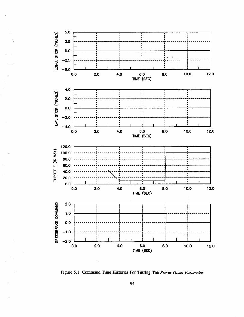
,m,-l-(bzV

v0

c+Z

q

5.0

2.5

0.0

-2.5

-5.00.0

0 II !

! I

,.*..--...... 6- ---..-------- .... --------*- -----------.I I

- I I! I

_ , : ,............ _........... ,'-..................... +- ......... F...........

I J I I I

I I I !

I : I ', I , I ', I I I

2.0 4.0 6.0 8.0 10.0 12.0_ME (SEC)

l.d-1-(3z

V

(.3

4.0

2.0

0.0

-2.0

-4.00.0

I I II I l l

I I I

I I I

I

, l l

I I I I I

I I I I I I I , I I I

2.0 4.0 6.0 8.0 10.0 12.0_ME (SEC)

120.0

I< 80.0

,., 60.0

o 40.0n-

2o.o0.0

T i 7

1 I TI I .

0 I I

I I I

I I I

I I I

0.0 2.0 4.0 6.0 8.0 10.0 12.0_ME (SEe)

_E0o

bJ

_D

P,bJ

U')

2.0

1.0

0.0

-1.0

-2.00.0

I ', : ', :I I I I I

I I I I I

I I I I ...... ****L ...........

I * i *I I

I I I I I I

I I I I I

I O I I I

I I I I I

I I I I I........... "i........... _ .......... T .......... -i ........... i" ...........

I

I I I I I I, I I I I I I I I I

2.0 4.0 6.0 8.0 10.0 12.0TIME (SEC)

Figure 5.1 Command Time Histories For Testing The Power Onset Parameter

94

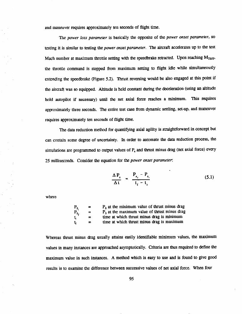
and maneuver requires approximately ten seconds of flight time.

The power loss parameter is basically the opposite of the power onset parameter, so

testing it is similar to testing the power onset parameter. The aircraft accelerates up to the test

Mach number at maximum throttle serdng with the speedbrake retracted. Upon reaching M_sr,

the throttle command is stepped from maximum setting to flight idle while simultaneously

extending the speedbrake (Figure 5.2). Thrust reversing would be also engaged at this point if

the aircraft was so equipped. Altitude is held constant during the deceleration (using an altitude

hold autopilot ff necessary) until the net axial force reaches a minimum. This requires

approximately three seconds. The entire test case from dynamic settling, set-up, and maneuver

requires approximately ten seconds of flight time.

The data reduction method for quantifying axial agility is straightforward in concept but

can contain some degree of uncertainty. In order to automate the data reduction process, the

simulations are programmed to output values of P, and thrust minus drag (net axial force) every

25 milliseconds. Consider the equation for the power onset parameter:

AP, = Ps,-P,, (5.1)

At tf - t i

where

PS. '-

Ps I =ti =

t_ =

Ps at the minimum value of thrust minus dragPs at the maximum value of thrust minus drag

time at which thrust minus drag is minimum

time at which thrust minus drag is maximum

Whereas thrust minus drag usually attains easily identifiable minimum values, the maximum

values in many instances are approached asymptotically. Criteria are thus required to define the

maximum value in such instances. A method which is easy to use and is found to give good

results is to examine the difference between successive values of net axial force. When four

95

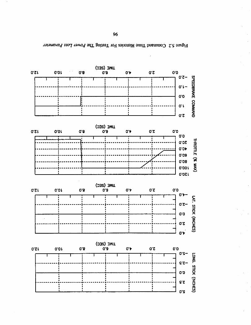
96

O'_t

I ; I ; I ; I ' I ; Ii I I !

I I I I

I I I II i l l

...........i..........JL i............ !!

$

• *** ................ **_ ...........

I ! I i

: ,' :

(03S)3rILL0"0t O'G 0"9 0"_ 0"2_ 0"0

o'z-

O,t- _0"0 m

oO't _=

0'_ _

(03S) 3riLL0"_t 0"0t O'G 0"9 0"_ 0"_ 0"0

0"0

qIIllIIIlill !llIIIIIII

I

I

) lllill III I _ I I I Illl _I li

)IIIIllllII_ililOIIIll( .IIIIIllIIl&lllillilIl_IllIIIIIIII_l IIillIll

O t O| !

IIIIIllllllJllIllIlllII DIIIIIIIIII_IIIIIIIIII_IIIIIIII

i I I ..........I I I I

I"

I

llililllili Ji ! I I!!! lili

.............................................. 0"02_| I

, ,...........°..........".......................0"0_

0"09 rn

0"09

o'ooL0"0_t

(o s)- ntt0"2:t 0"0 t 0"9 0"9 O'tr O'g 0"0

I ' ; I ; I I ; I ; I O'Ir--

I I III I

I I........... t ........... c..................... -,........... I-........... 0"_-I ! I

: : , I : O'O

I I II I I

! I ! 0"t_

(-)x

z<-)-r

(03S) 3_110"_ t 0"0 t 0"9 0"9 0"_ 0"2: 0"0

I ; I ; I ; I ; I ; I: ,' : : : -

I I........... t ........... c .......... ÷.......... -,........... t"...........I I I I

I I I I

I ! I e

I I I I II I I I

I I I I

I I I I i

I ! i I

I I I I

I I O I

O'_w

g'_-

0"0

O'g

z.o

o

zow,

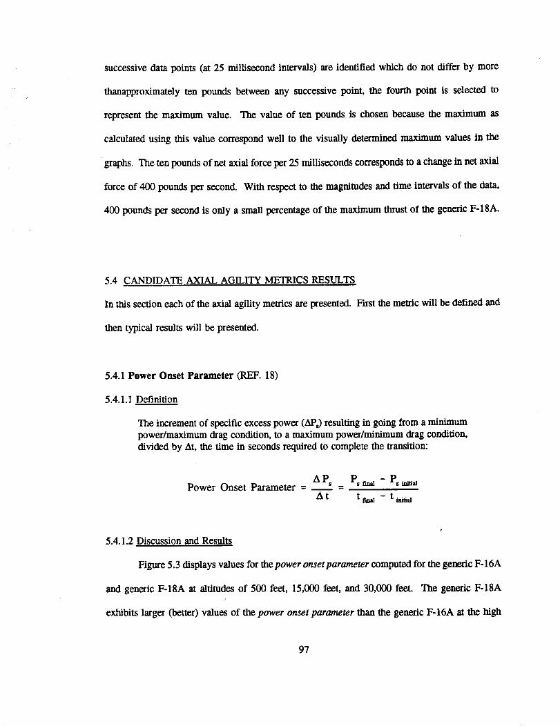
successive data points (at 25 millisecond intervals) are identified which do not differ by more

thanapproximately ten pounds between any successive point, the fourth point is selected to

represent the maximum value. The value of ten pounds is chosen because the maximum as

calculated using this value correspond well to the visually determined maximum values in the

graphs. The ten pounds of net axial force per 25 milliseconds corresponds to a change in net axial

force of 400 pounds per second. With respect to the magnitudes and time intervals of the data,

400 pounds per second is only a small percentage of the maximum thrust of the generic F-18A.

5.4 CANDIDATE AXIAL AGILITY METRICS RESULTS

In this section each of the axial agility metrics are presented. First the metric will be defined and

then typical results will be presented.

5.4.1 Power Onset Parameter (REF. 18)

5.4.1.1 Definition

The increment of specific excess power (AP_) resulting in going from a minimum

power/maximum drag condition, to a maximum power/minimum drag condition,divided by At, the time in seconds required to complete the transition:

A PsPower Onset Parameter = __ =

At t_ - t_

5.4.1.2 Discussion and Results

Figure 5.3 displays values for the power onset parameter computed for the generic F-16A

and generic F-18A at altitudes of 500 feet, 15,000 feet, and 30,000 feet. The generic F-18A

exhibits larger (better) values of the power onset parameter than the generic F-16A at the high

97

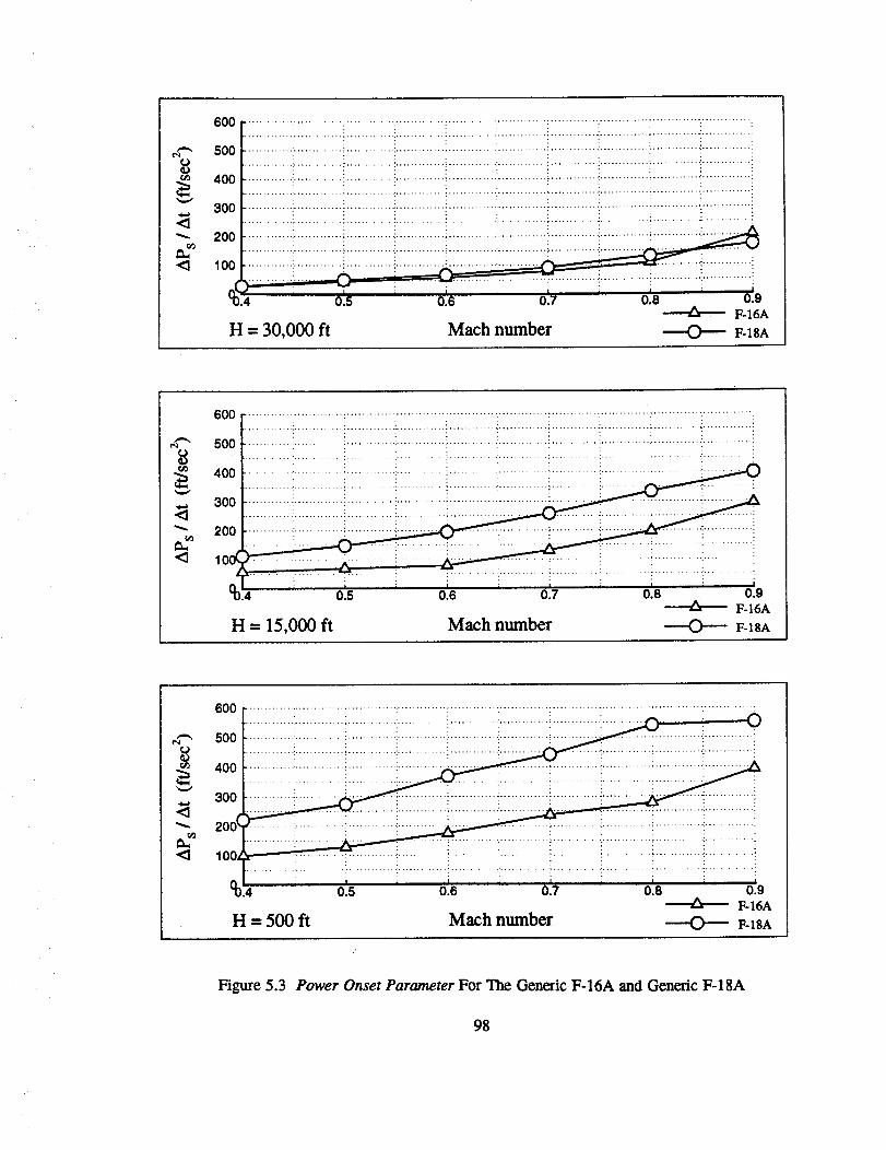
8

r_

600 ............. ,........................... .............. :..............................................................................

500 ......................................... :............. ?......................................................................................................................... i............. .'-................................................................................

400 ........................................ !............. _................................................................................

300 ........................................::......................................... i............ :............. ;.......................... :

............ i............. : ............. !............. i ............. !............. i _i............. !.................. i_oo•...........i............±............i.........._ .........i........_ .....i

"D 4 0 5 0 6 0.7 0.8 0.9• " " _ F-16A

H = 30,000 ft Math number ---O---- l_-18A

600 ......................................................:..........................:.............,.............:.............•.............:.......................................-.............i...........................i............-.............i............-..............

500 .............:..........................._.............!............._.............?.............i.............;............._............:...........:....................i........i.........:........_.........._.......... !.........:

_ i i i " ! : ........ i....................... :............. !

°o., " o!s ' o_._ _ o'.7 : o._ ' o.9F-16A

H = 15,000 ft Mach number --O--- F-ZSA

600 ...........................:.............:...........................:.............:............_.............:............_.............:

.........................._.............i............._..........................:_.............::............_.......:, "0500

400

g300

2od

_ 100, - :........... :............ :............. _........................... _............. :............. _ ........ :............. :

............ i............. i............. i............. : .......... :............ : ............. :........... : ....... i............ :

{_,. , , , i , , , , , ,4 0.5 0.6 0.7 0.8 0.9F-I6A

H = 500 ft Math number ----O--- F-ISA

Figure 5.3 Power Onset Parameter For The Generic F-16A and Generic F-18A

98

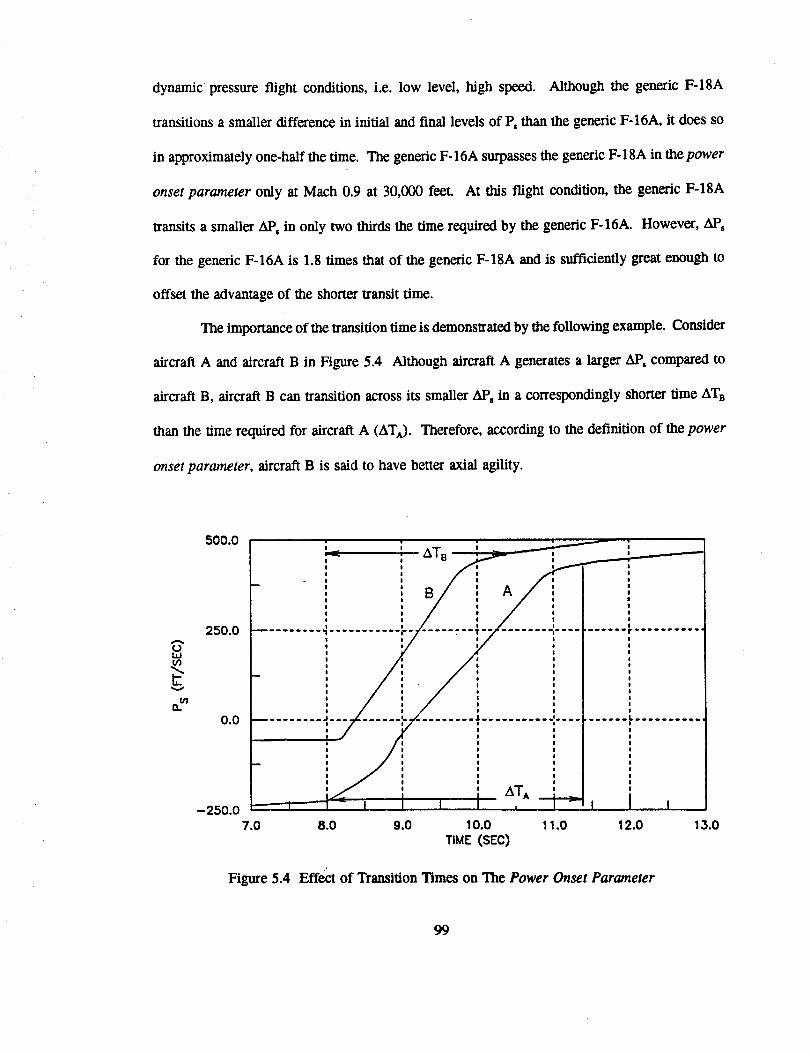
dynamic pressure flight conditions, i.e. low level, high speed. Although the generic F-18A

transitions a smaller difference in initial and final levels of P, than the generic F-16A, it does so

in approximately one-half the time. The generic F-16A surpasses the generic F-18A in the power

onset parameter only at Mach 0.9 at 30,000 feet. At this flight condition, the generic F-18A

transits a smaller AP, in only two thirds the time required by the generic F-16A. However, AP,

for the generic F-16A is 1.8 times that of the generic F-18A and is sufficiently great enough to

offset the advantage of the shorter transit time.

The importance of the transition lime is demonstrated by the following example. Consider

aircraft A and aircraft B in Figure 5.4 Although aircraft A generates a larger AP, compared to

aircraft B, aircraft B can transition across its smaller AP, in a correspondingly shorter time ATB

than the time required for aircraft A (AT^). Therefore, according to the definition of the power

onset parameter, aircraft B is said to have better axial agility.

t.bI.dt/)

tn

500,0

250.0

0.0

-250.0

- I I I I I

m i I ¢ I |

I !

' ./.. i../...i 'I | e i 1

i i i ! i

i i il I i

I ! ! I I

......... _ ........... F" -- ................. r ...........

| I I I I

I I I

I I I I I

I I I I 1

e i I I II I O 8 O

I I " I I II I I I I

I I I I II ! I t I

I ! I I I

I I I I I,, ,// ,,I I I I I

I I ! I I

I I I I !

i I I I I I

I I I I I

I I I I I

I I I I I

O l I t I,./i i T.L,

- I --i_ I I I I , I _ I ! I

7.o 8.o 9.o 1o.o __.o 12.0 __.oT_ME(sEc)

Figure 5.4 EffeJzt of Transition Times on The Power Onset Parameter

99

5.4.1.3Summary

The power onset parameter is simple to test, but measurement of the final Ps level can

be difficult in certain cases. The initial or final value of P, itself usually does not dominate this

metric, but the transition times between the initial and final values usually does. In a few

situations the value AP_ can be important, but normally to a lesser extent.

5.4.2 Power Loss Parameter (REF. 18)

5.4.2.1 Definition

The increment of specific excess power (AP,) resulting in going from a maximum

power/minimum drag condition, to a minimum power/maximum drag condition,

divided by At, the time in seconds required to complete the transition:

APPower Loss Parameter = __ =

At

Ps final - Ps initial

tf,_ - tim,,

5.4.2.2 Discussion and Results

Figure 5.5 displays values for thepower loss parameter for the genetic F-16A and generic

F-18A at altitudes of 500 feet, 15,000 feet and 30,000 feet. Note that unlike the results for the

power onset parameter, Figure 5.5 shows that the generic F-18A does not have better axial agility

than the generic F-16A over most of the test points. At all altitudes, the generic F-18A is superior

in the low subsonic Mach number range, while the generic F-16A is superior in the high subsonic

Mach range. The generic F-18A achieves both larger differences in P, levels and shorter transition

times than the generic F-16A over all low subsonic Mach numbers, at all the altitudes tested. The

power loss parameter values for the two aircraft are similar at 0.7 Math at 500 feet and 15,000

feet, after which the generic E-16A is able to transition a larger AP, and having a shorter transition

100

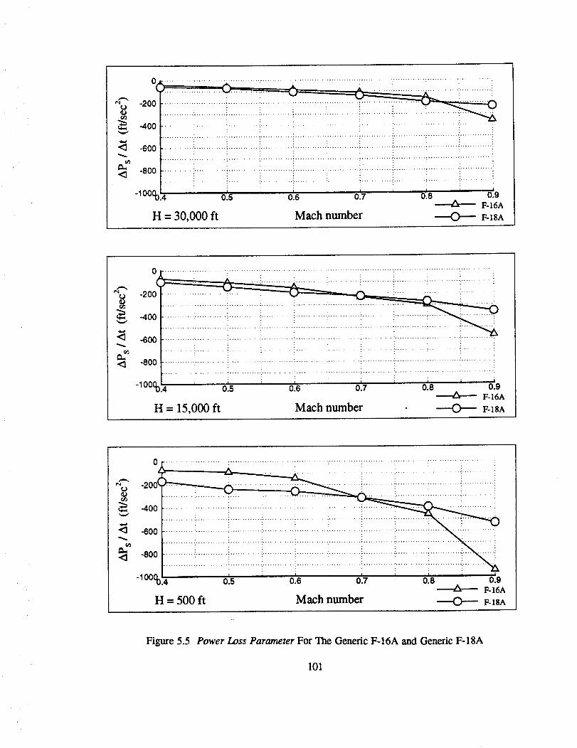
-400

'_ -600

r_

-lOOOo,4 ,

H = 30,000 ft

)!'iiiii................._iiii ....ii............._iiiiiiiiiiiiiiiiiiiiiiiiiiiiiiiiiiiilliiiiiiiiiiiiiiii

iiii i i iiiiiii i......... ii iii iii ii !iiiiiiii i iiiiii ... ........ : .... : ..........

............ i........... : ............. _............. : ............. i- i : i

............ ............. i ....................................... :............. ; ......................... ! ............. !............. :

.:............. ; .......... :............. _............. _............. i

, i I , i i , i i0.5 0.6 0.7 0.8 0.9

F-16A

Mach number ----O--- F-]SA

r_

-400

<1 -600

-_OOOo'.,)

i iiiiiliiiiiiii.... : i ! i i i

....................................... ::............ _ ...................... _........... i............. _............. !.......... :; i _ : i i i ,o.s o'._ o17 o.8 o.o

F-16A

Mach number _ F-laAH = 15,000 ft

0

-2od

-400

-600

_-'_ -800

-10000'.4 '

H = 500 ft

i iiiiiiiiiiI i I , I i I i I

0.5 0.6 0.7 0.8 0.9F-16A

Math number ----O---- F-]sA

Figure 5.5 Power Loss Parameter For The Generic F-I6A and Generic F-18A

101

time than the generic F-18A. The generic F-16A is superior at 30,000 feet only because of its

larger Ps level.

5.4.2.3 Summary

Although the power loss parameter is very similar to the power onset parameter, the

results have shown that an aircraft which is superior in terms of one of the axial agility metrics

is not necessarily superior in terms of the other metric also. The power loss parameter is simple

to test, and is generally affected by the same parameters as the power onset parameter.

5.5 SUMMARY

Axial agility metrics measure the capability of an aircraft to transition between maximum

and minimum Ps levels. Instead of knowing only what level of Ps an aircraft possesses at a

particular point, axial agility reflects how fast the aircraft can transition to another P, level. The

time required to make the transition tends to be the most important aspect, while the magnitude

of the P_ change involved in transitioning is important to a lesser extent. Thus both the time rate

of change of thrust and the time rate of change of drag are influential. Overall, the time rate of

change of thrust, i.e. engine spool time, tends to have a more pronounced effect on these metrics

than the time rate of change of drag, i.e. effectiveness and deployment times of speedbrakes. In

terms of axial agility, an agile aircraft is characterized as having high thrust engines with very

short spool times, and fast deploying, effective speedbrakes.

The power onset parameter and power loss parameter are not measures of the acceleration

capability of an aircraft. In fact, the acceleration of the aircraft has a negligible impact on the

values of the power onset parameter and power loss parameters, meaning that the weight of the

102

aircraftdoesnotaffectthevalues(AppendixD). Therefore,a lighter aircraft is not advantageous

in terms of axial agiliW.

The axial agility of a fighter is also affected by the engine's transient performance at

elevated angles of attack and sideslip. The transient behavior of the engine during large scale

maneuvers and high angle of attack flight is an important contributor to overall combat

effectiveness. However, the power onset parameter and the power loss parameter do not address

this aspect of engine performance.

The power onset parameter and power loss parameter could be easily extended tO.account

for any unique capabilities which may be used to effect changes in Ps. These capabilities may

consist of engines with very fast response to throttle commands, thrust vectoring or thrust

reversing nozzles, or even nozzles which permit vectoring in forward flight (VIFFING).

103

6. FUNCTIONAL AGILITY

6.1 BACKGROUND

Functional agility metrics are intended to quantify how fighter aircraft execute rapid

changes in heading or rotations of the velocity vector. This class of metrics is concerned with a

time scale on the order of ten to twenty seconds. These metrics as a class tend to place emphasis

on energy lost during turns through large heading angles, and the time required to recover kinetic

energy after unloading to zero normal load factor. Many of the functional agility metrics involve

maneuvers composed of brief transient segments. The effect of these transient segments are

measured best by the class of transient agility metrics, e.g. pitch agility and lateral agility.

However, metrics are needed to quantify an entire maneuver. These are the functional agility

metrics.

This chapter demonstrates how to test, measure, and compare the functional agility of

fighter aircraft using several of the candidate functional agility metrics. For the results contained

in this chapter, functional agility is quantified using nonlinear, non real-time, six degree-of-

freedom generic flight simulation computer programs. Results and analysis are presented for the

F-5A, F-16A, F-18A, and X-29A aircraft to show how characteristics of the aircraft and flight

control system (FCS) can influence the metrics. The maneuvers and results are intended to

quantify the agility of the aircraft being tested. The acceptability of such maneuvers to an

operational pilot, the associated issues of flying qualities, pilot discomfort, and g-induced loss of

consciousness are not addressed in this report.

104

6.2 CANDIDATE FUNCTIONAL AGILITY METRICS

In recent years agility researchers have proposed numerous metrics to quantify functional

agility of fighter aircraft. The proposed metrics include:

1)

2)

3)

4)

5)

6)

7)

8)

9)

combat cycle time 1800 heading change

combat cycle time 90 ° heading change

dynamic speed turn

relative energy state

energy-agility concept

time-energy penalty

DT parameter

pointing margin

one-circle pointing quotient

All nine candidate functional agility metrics are defined in Appendix A. Results for the DT

parameter, pointing margin, and one-circle pointing quotient metrics are not presented in the

current study, since these metrics have been previously analyzed and tested. For a discussion and

results from these metrics, the reader should consult References 35, 30, and 41 respectively.

6.3 FUNCTIONAL AGILITY TESTING AND DATA REDUCTION TECHNIQUES

Metrics one through six listed above are tested at Mach equals 0.8 at 15,000 feet. The

Mach number is selected to at or near comer speed for the aircraft tested, and the altitude is

selected to be representative of that at which fighter aircraft are most likely be engaged in within

105

visualrangeaircombat.Themaneuversequenceusedto test the combat cycle time metric (CCT)

is sufficient for testing the dynamic speed turn, relative energy state, energy-agility concept, and

time-energy penalty metrics. Data for all of these metrics can be obtained by post-processing a

single CCT test case for a given aircraft.

Although not explicitly a part of the clef'tuition of any metric, a set of constraints is

established in order to define an acceptable or realistic maneuver. This consideration is

particularly important for the functional agility metrics from an energy management standpoint.

The constraints also provide a level of standardization and repeatability. Referring to Figure 6.1,

the CCT metric is a series of segments consisting of the time to pitch from one g to the limit

normal load factor (t_), plus the time to turn to a specified new heading angle at maximum normal

load factor (t_ + t22), plus the time to unload the aircraft to a normal load factor of either one or

zero (t3), plus the time to accelerate to the original energy level (t,). The enforced test constraints

for the CCT maneuver sequence consist of the following:

°

2.

3.

altitude excursion during any phase: ± 1500 feet

altitude excursion during unload and roll: ± 200 feet

captured heading angle excursion: ± 5 °

The altitude band is imposed during the transition from the unloading phase (t_) to the start of the

acceleration phase (t4) to insure that the aircraft is using a straight-line acceleration to regain the

original energy, and not climbing to gain altitude or descending to gain airspeed. Tiffs isolates

the ability of the aircraft to accelerate without using beneficial gravity effects. The heading angle

capture criterion of ±2 ° is arbitrarily selected, and insures that the acceleration phase of the

maneuver occurs at the desired heading.

106

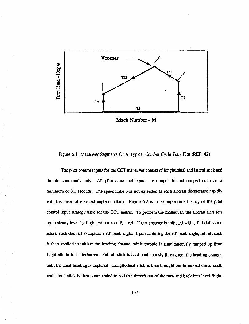
o

o

E

'I"3

Vcomor /

T1

T4

Mach Number- M

Figure 6.1 Maneuver Segments Of A Typical Combat Cycle Time Plot (REF. 42)

The pilot control inputs for the CCT maneuver consist of longitudinal and lateral stick and

throttle commands only. All pilot command inputs are ramped in and ramped out over a

minimum of 0.1 secor.ds. The speedbrake was not extended as each aircraft decelerated rapidly

with the onset of elevated angle of attack. Figure 6.2 is an example time history of the pilot

control input strategy used for the CCT metric. To perform the maneuver, the aircraft first sets

up in steady level lg flight, with a zero P_ level. The maneuver is initiated with a full deflection

lateral stick doublet to capture a 90 ° bank angle. Upon capturing the 90 ° bank angle, full aft stick

is then applied to initiate the heading change, while throttle is simultaneously ramped up from

flight idle to full afterburner. Full aft stick is held continuously throughout the heading change,

until the final heading is captured. Longitudinal stick is then brought out to unload the aircraft,

and lateral stick is then commanded to roll the aircraft out of the turn and back into level flight.

107

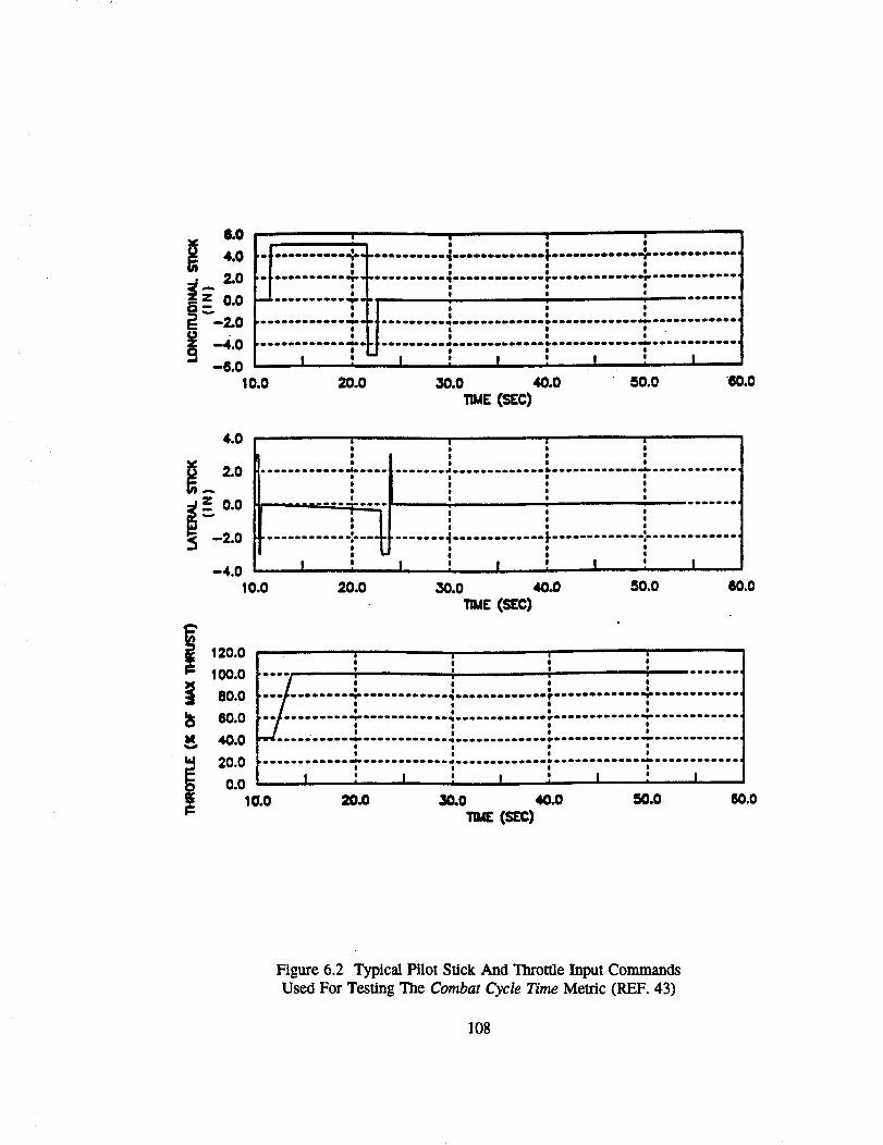
,*.0°

10.0 20.0 30.0 40.0 50.0 60.0_[ (sEc)

4.0

2.O

-2.0

-4.010.0

120.0

100.0

80.O

60.0

40.0

20.00.0

: : : :

: t : : :

oeoeee_ei_e_ee_ e _ e e e o o _ eee O_ _ _ _e _ e ee_e e e_e _ _ e OIBIP_ _"'11" e _ e e _ e e_ _ _ _ _ '

* 0 e $

I I I I

I t * e

O * e e.... ...oo4. oo_ , . n iooo*o*o,

T 7 ; ; *I O II *

O t

O II O e 0

I v_ I O I

| o i* | o, I , ! _ !

2o.o _o.o 4o.o so.o oo.o

e l o

o e i

ooo e ! * OODB_I

" /. ; ; ; ;I | I i

_ e e I e

O o I e

eo ooooooo_o_o_oooo_ooo_Dqool.omoomooooo _omenooo_eDeeoe_ooo_ooooo_ooq

e I I I "

• O I P I

_ oiII, eIOIIe! I iiloi t emqlOeOoi_,iImOelipo IOeOIIlIl'l'oIieellloIIel o4

t * e0 I *

............ "7............ _.......................... "7.............j , o, l : I , I , I

lO.O 2o.0 _o 40.0 5o.o _.o(sic)

Figure 6.2 Typical Pilot Stick And Throttle Input Commands

Used For Testing The Combat Cycle Time Metric (REF. 43)

108

Heading angle change is the independent variable for selecting test points for the CCT

metric. Heading angle changes of 180 ° and 90 ° are selected for this study. A 180 ° heading

change is selected because previous studies involving minimum time turns consider 180 ° heading

changes as a baseline maneuver (REF. 44, 45, 46). A 90° heading angle change is selected as an

attempt to reduce the influence of sustained maneuvering.

The dynamic speed turn plots are by definition cross-plots from the

energy-maneuverability doghouse plot (REF. 47). Rather than developing the entire

energy-maneuverability diagram for each aircraft, the turn rate versus airspeed data from the CCT

maneuver is used to obtain data for this metric. The equation for specific excess power (P_) is

used to calculate the amount of acceleration and deceleration. Since the CCT maneuver does not

employ a level turn, the acceleration and bleed rates for the dynamic speed turn plots are

calculated by differentiating true airspeed in knots. Airspeed changes are indicated using Mach

number.

The data for the relative energy state metric is obtained from the CCT maneuver by

dividing the velocity of the aircraft during the turn by the corner velocity (V_). It is suggested

that at least two 90 ° turns be completed before the velocity of the aircraft falls below corner speed.

The energy-agility plot is generated by plotting P_ as a function of time during the CCT

The time to kill (tk) is then defined as the time required to reach a heading angle ofmaneuver.

180 °.

The generic F-18A simulation is used to assess the sensitivity of the functional agility

metrics. It is important to note that these sensitivity results are specific to the generic F-18A only,

and cannot be generalized to all fighter aircraft. The intent here is simply to determine in a

broad sense how sensitive the functional agility metrics can be to pilot inputs, and to demonslrate

one way in which an analysis of this type can be conducted. Since this analysis is simply

109

intended to show typical behavior, the sensitivity tests are limited to a single altitude of 15,000

feet.

The sensitivities are determined by generating optimal trajectories for the 1800 and 90 °

CCT maneuvers using the Optimal Trajectories by Implicit Simulation (OTIS) program (Appendix

B). Angle of attack and bank angle are the conlrol parameters which the OTIS program uses to

generate the optimal CCT maneuver. The angle of attack and bank angle time histories specified

by the OTIS program are then used as schedules for determining a sequence of pilot stick input

commands. This command sequence is then used to reproduce the optimal CCT maneuver using

the generic F-18A simulation. The optimal CCT maneuver is also used to determine sensitivities

for the dynamic speed turn, relative energy state, energy-agility concept, and time energy penalty

metrics.

Three variations of the 180 ° and 90 ° CCT maneuvers form the basis for the sensitivity

analysis:

1)

2)

3)

heading change at maximum angle of attack

optimal turn; defined here as a minimum time mm without thefinal velocity defined, and using the angle of attack schedule

specified by OTIS

optimal total time; defined here as a minimum time turn with the

final velocity = initial velocity, and using angle of attack

schedule specified by OTIS

The comtraints enforced on the nominal CCT are applied to the three maneuvers listed above.

The first variation, heading change at maximum angle of attack, is tested by maintaining full aft

stick deflection after the aircraft captures the initial 90° bank angle, until the aircraft achieves the

new heading. A full aft stick deflection is typically used in flight testing agility parameters (REF.

25, 48).

110

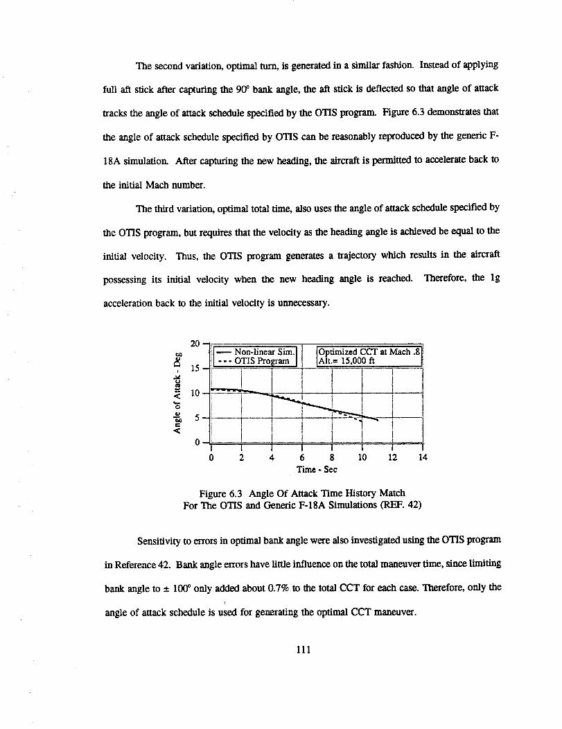
The second variation, optimal turn, is generated in a similar fashion. Instead of applying

full aft stick after capturing the 90 ° bank angle, the aft stick is deflected so that angle of attack

tracks the angle of attack schedule specified by the OTIS program. Figure 6.3 demonstrates that

the angle of attack schedule specified by OTIS can be reasonably reproduced by the generic F-

18A simulation. After capturing the new heading, the aircraft is permitted to accelerate back to

the initial Mach number.

The third variation, optimal total time, also uses the angle of attack schedule specified by

the OTIS program, but requires that the velocity as the heading angle is achieved be equal to the

initial velocity. Thus, the OTIS program generates a trajectory which results in the aircraft

possessing its initial velocity when the new heading angle is reached. Therefore, the lg

acceleration back to the initial velocity is unnecessary.

!

t_

<

o

<

0 u

[m Non-linear Sim.I i IOptimized CCT at Mach .8 i

--- OTIS Pro_am J! IAlt.= 15,000 ft [15.......................i....................._.................i............i.................!................]................]10 -- _"........................... _ :' *' i i ........I

5 -- : _ *' T -_"_"_-- •.... ,! i i i , i t

0_ i 1 i i i II I I I I I I

0 2 4 6 8 10 12 14

Time - Sec

Figure 6.3 Angle Of Attack Time History MatchFor The OTIS and Generic F-18A Simulations (REF. 42)

Sensitivity to errors in optimal bank angle were also investigated using the OTIS program

in Reference 42. Bank angle errors have little influence on the total maneuver time, since limiting

bank angle to _ 100 ° only added about 0.7% to the total CCT for each case. Therefore, only the

angle of attack schedule is used for generating the optimal CCT maneuver.

111

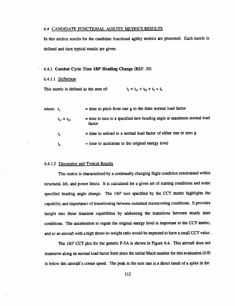
6.4 CANDIDATE FUNCTIONAL AGILITY METRICS RESULTS

In this section results for the candidate functional agility metrics are presented.

defined and then typical results are given.

Each metric is

6.4.1 Combat Cycle Time 180" Heading Change (R.EF. 30)

6.4.1.1 Definition

This metric is defined as the sum of: t_ + t2_ + h_ + h + t4

where

h

h

= time to pitch from one g to the limit normal load factor

= time to turn to a specified new heading angle at maximum normal loadfactor

= time to unload to a normal load factor of either one or zero g

= time to accelerate to the original energy level

6.4.1.2

structural, lift, and power limits.

specified heading angle change.

Discussion and Typical Results

This metric is characterized by a continually changing flight condition constrained within

It is calculated for a given set of starting conditions and some

The 180 ° turn specified by the CCT metric highlights the

capability and importance of transitioning between sustained maneuvering conditions. It provides

insight into these transient capabilities by addressing the transitions between steady state

conditions. The acceleration to regain the original energy level is important to the CCT metric,

and so an aircraft with a high thrust-to-weight ratio would be expected to have a small CCT value.

The 180 ° CCT plot for the generic F-5A is shown in Figure 6.4. This aircraft does not

maneuver along its normal load factor limit since the initial Mach number for this evaluation (0.8)

is below this aircraft's comer speed. The peak in the turn rate is a direct result of a spike in the

112

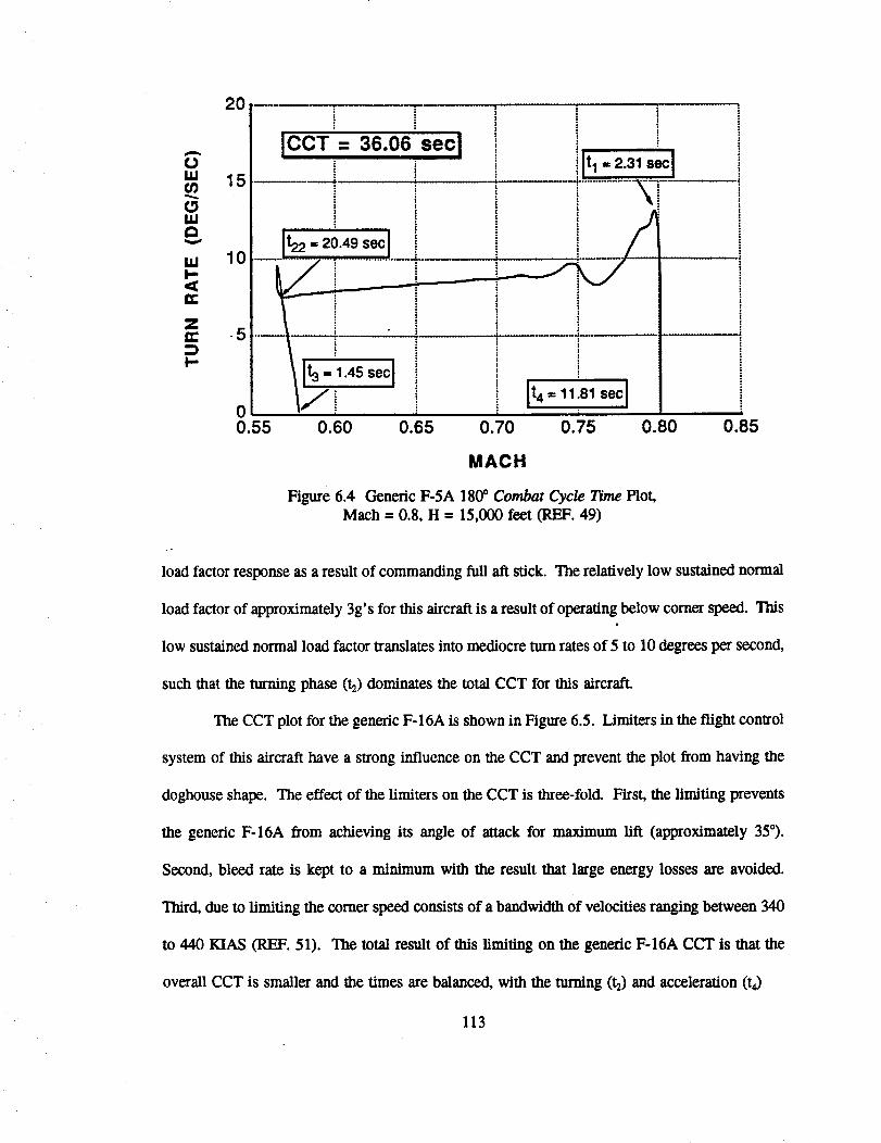
Oi11t/)

OtU

IllI--

a"

Zer"

i--

°L15

10

-5

ICCT = 36.06 secJ

t22 = 20.49 sec I

...................i.......'

_= il .45 secl

Vj

ilt,

i

0.55 0.60 0.65 0.85

t = 11.81 secJi

0.70 0.75 0.80

MACH

Figure6.4 GenericF-5A 180° Combat Cycle Time Plot,

Mach = 0.8,H = 15,000feet(REF. 49)

load factor response as a result of commanding full aft stick. The relatively low sustained normal

load factor of approximately 3g's for this aircraft is a result of operating below comer speed. Tiffs

low sustained normal load factor translates into mediocre turn rates of 5 to 10 degrees per second,

such that the turning phase (ta) dominates the total CCT for this aircraft.

The CCT plot for the generic F-16A is shown in Figure 6.5. Limiters in the flight control

system of this aircraft have a strong influence on the CCT and prevent the plot from having the

doghouse shape. The effect of the limiters on the CCT is three-fold. First, the limiting prevents

the generic F-16A from achieving its angle of attack for maximum lift (approximately 35°).

Second, bleed rate is kept to a minimum with the result that large energy losses are avoided.

Third, due to limiting the comer speed consists of a bandwidth of velocities ranging between 340

to 440 KIAS (REF. 51). The total result of this limiting on the generic F-16A CCT is that the

overall CCT is smaller and the times are balanced, with the turning (t2) and acceleration (t4)

113

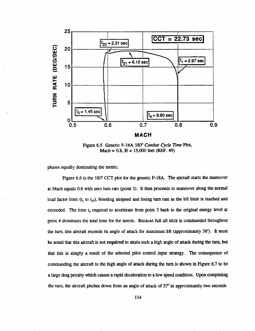
25

A

C_W

r_I.U

U.II-<rr"

Z

I-

20

15

10

5

0

It22 = 2.31 sec IICCT = 22.73 sec !

ilt,-2,Ts.ol

t = 9.90 sec I

0.5 0.6 0.7 0.8 0.9

MACH

Figure 6.5 Generic F-I6A 180 ° Combat Cycle Time Plot,Mach ffi0.8, H = 15,000 feet (REF. 49)

phases equally dominating the metric.

Figure 6.6 is the 1800 CCT plot for the generic F-18A. The .aircraft starts the maneuver

at Mach equals 0.8 with zero turn rate (point 1). It then proceeds to maneuver along the normal

load factor limit (tl to ta2), bleeding airspeed and losing turn rate as the lift limit is reached and

exceeded. The time t4 required to accelerate from point 3 back to the original energy level at

point 4 dominates the total time for the metric. Because full aft stick is commanded throughout

the turn, this aircraft exceeds its angle of attack for maximum lift (approximately 38°). It must

be noted that this aircraft is not required to attain such a high angle of attack during the turn, but

that this is simply a result of the selected pilot control input strategy. The consequence of

commanding the aircraft to the high angle of attack during the turn is shown in Figure 6.7 to be

a large drag penalty which caUses a rapid deceleration to a low speed condition. Upon completing

the turn, the aircraft pitches down from an angle of attack of 57 ° in approximately two seconds

114

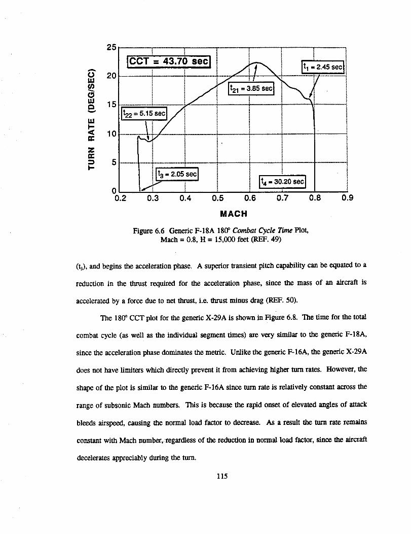
25

A

OW

O!11t_

IllI--

Z

I--

20

15

10

5

ICCT = 43.70 sec I

t22 = 5.15 sec I

t21 = 3.85 sec I

t = 30.20 sec I

0.6 0.7

MACH

Figure 6.6 Generic F-18A 1800 Combat Cycle Time Plot,Mach= 0.8, H = 15,000 feet (REF. 49)

(h), and begins the acceleration phase. A superior Iransient pitch capability can be equated to a

reduction in the thrust required for the acceleration phase, since the mass of an aircraft is

accelerated by a force due to net thrust, i.e. thrust minus drag (REF. 50).

The 180 ° CCT plot for the generic X-29A is shown in Figure 6.8. The time for the total

combat cycle (as well as the individual segment times) are very similar to the generic F-18A,

since the acceleration phase dominates the metric. Unlike the generic F-16A, the generic X-29A

does not have limiters which directly prevent it from achieving higher turn rates. However, the

shape of the plot is similar to the generic F-16A since turn rate is relatively constant across the

range of subsonic Mach numbers. This is because the rapid onset of elevated angles of attack

bleeds airspeed, causing the normal load factor to decrease. As a result the turn rate remains

constant with Mach number, regardiess of the reduction in normal load factor, since the aircraft

decelerates appreciably during the turn.

115

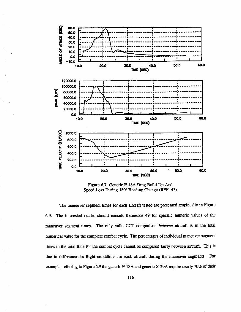
_O

40.0

30.020.0100

O0-IO0I_o 20o- _o.o 40o so.o eo.o

T._ (S_C)

120000.0 ....O I I I1ooooo.0 ....... _,,._-- -,'-............ .I............. F............ -:-............

' 'I----_.""""'""1_1(:_10.0 .......... .... ° ..... ...... °''0""

I ! "_1 o o o uO e o

o e o

e o o

0000eO _ go ° °Io ° I° q_e_°IOl° °eeoepoooll °°oee_e_ooleooe° _ol°

I I lt I t

I I I

_ t ! ! --0.0 , 1 I , Ilo.o 2o.o _o 4o.o _.o _.o

T_ (S(C)

1000.0 ' ' ' ' t

$ I 0 |I O O I

00o0 i oloomI_owlloo mloloodmoooIoomoloIiA-ooooooooloo _ooooooloooI I O I

g O O I

I e I I

I .................................................... 1

I ¢ 8 O

¢ O . O t

I t I 8 _00o o °coJ Jq,_ _ql4JUoU .ooooeoooooo eo .oooo .o°oo e oe °

I e o=oo.o ......... .:,"............e I I I

O t O I

O01oo 2o.o _o.o 40o 5o.o eo.o

Figure 6.7 Generic F-18A Drag Build-Up AndSpeed Loss During 180 ° Heading Change (REF. 43)

The maneuver segment times for each aircraft tested are presented graphically in Figure

6.9. The interested reader should consult Reference 49 for specific numeric values of the

maneuver segment times. The only valid CCT comparison between aircraft is in the total

numerical value for the complete combat cycle. The percentages of individual maneuver segment

times to the total time for the combat cycle cannot be compared fairly between aircraft. This is

due to differences in flight.conditions for each aircraft during the maneuver segments. For

example, referring to Figure 6.9 the generic F-18A and generic X-29A require nearly 70% of their

116

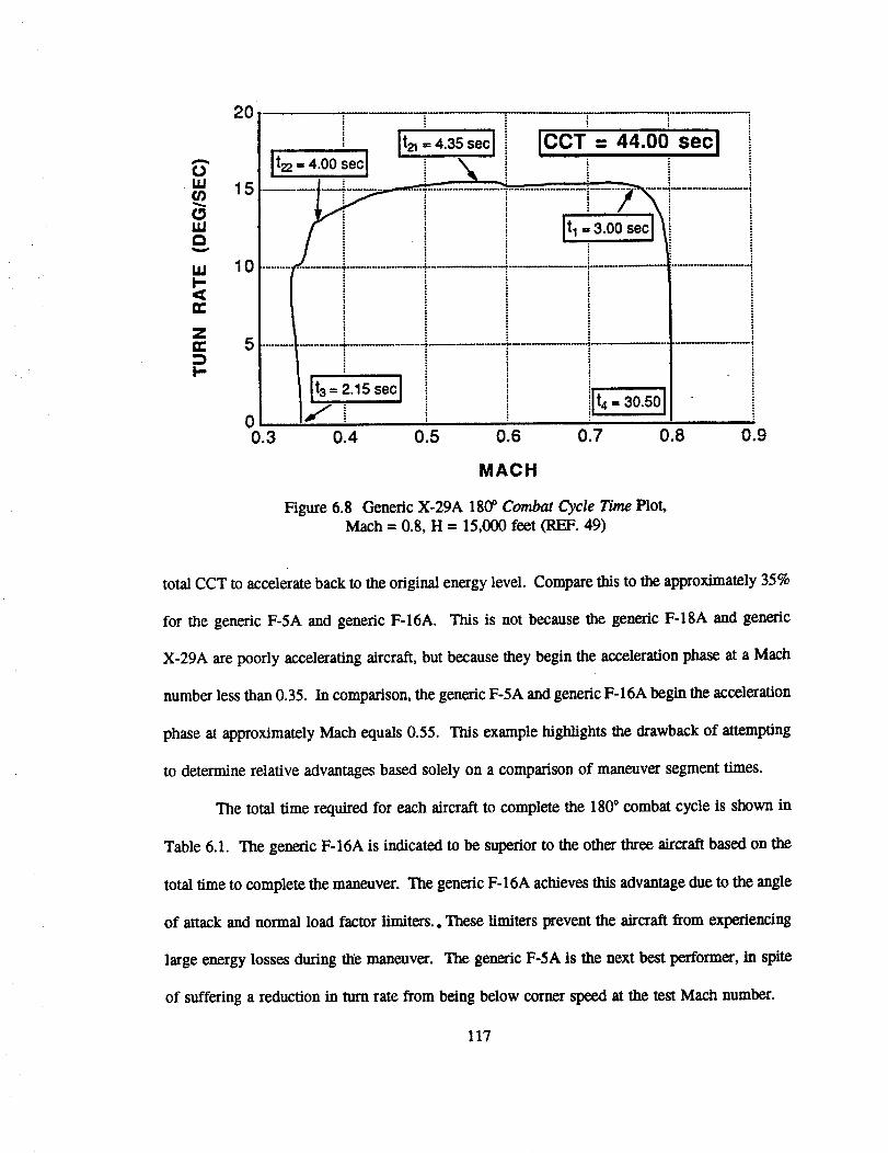
Orid

OIlle_

ulI--

Z

i--

20

15

10

5

0

It= '='°°secl It_=4.ZSsecI ICCT = 44.00 secI= \

......... ! i__

0.3 0.4 0.5 0.6 0.7 ).8

MACH

Figure 6.8 Generic X-29A 180 ° Combat Cycle Time Plot,Mach= 0.8, H = 15,000 feet (REF. 49)

0.9

total CCT to accelerate back to the original energy level. Compare this to the approximately 35%

for the generic F-5A and generic F-16A. This is not because the generic F-18A and generic

X-29A are poorly accelerating aircraft, but because they begin the acceleration phase at a Mach

number less than 0.35. In comparison, the generic F-5A and generic F-16A begin the acceleration

phase at approximately Mach equals 0.55. This example highlights the drawback of attempting

to determine relative advantages based solely on a comparison of maneuver segment times.

The total time required for each aircraft to complete the 1800 combat cycle is shown in

Table 6.1. The generic F-16A is indicated to be superior to the other three aircraft based on the

total time to complete the maneuver. The generic F-16A achieves this advantage due to the angle

of attack and normal load factor limiters.. These limiters prevent the aircraft from experiencing

large energy losses during the maneuver. The generic F-5A is the next best performer, in spite

of suffering a reduction in turn rate from being below corner speed at the test Mach number.

117

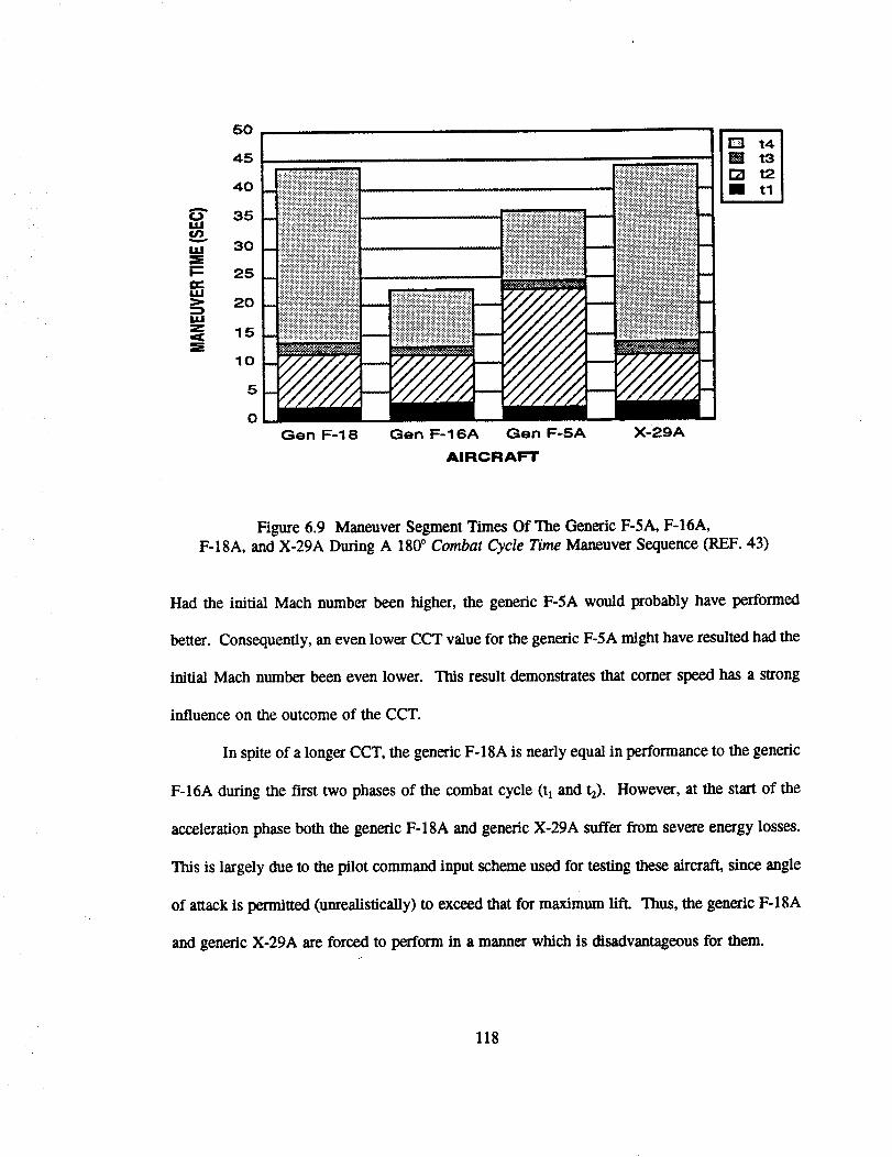
,45 :=: ::::::: i:i:i-i:ii

,o iiiiii ii iiiiiiiiii iii

15

Gen F-18 Gen 1::-16A Gen F-5A X-29A

AIRCRAFT

Figure 6.9 Maneuver Segment Times Of The Generic F-5A, F-16A,

F-18A, and X-29A During A 180 ° Combat Cycle Time Maneuver Sequence (REF. 43)

Had the initial Mach number been higher, the generic F-5A would probably have performed

better. Consequently, an even lower CCT value for the generic F-5A might have resulted had the

initial Mach number been even lower. This result demonstrates that comer speed has a strong

influence on the outcome of the CCT.

In spite of a longer CCT, the generic F-18A is nearly equal in performance to the generic

F-16A during the first two phases of the combat cycle (tl and t2). However, at the start of the

acceleration phase both the generic F-18A and generic X-29A suffer from severe energy losses.

This is largely due to the pilot command input scheme used for testing these aircraft, since angle

of attack is permitted (unrealistically) to exceed that for maximum lift. Thus, the generic F-18A

and generic X-29A are forced to perform in a manner which is disadvantageous for them.

118

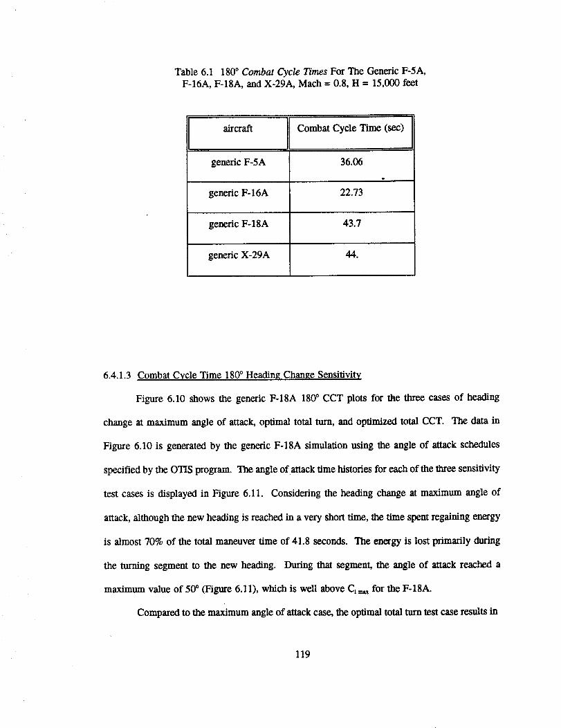
Table 6.1 180 ° Combat Cycle Times For The Generic F-5A,F-16A, F-18A, and X-29A, Mach= 0.8, H = 15,000 feet

aircraft Combat Cycle Time (see)

generic F-5A 36.06

generic F-16A 22.73

generic F-18A 43.7

generic X-29A 44.

6.4.1.3 Combat Cycle Time 180 ° Heading Change Sensitivity

Figure 6.10 shows the generic F-18A 180 ° CCT plots for the three cases of heading

change at maximum angle of attack, optimal total turn, and optimized total CCT. The data in

Figure 6.10 is generated by the generic F-18A simulation using the angle of attack schedules

specified by the OTIS program. The angle of attack time histories for each of the three sensitivity

test cases is displayed in Figure 6.11. Considering the heading change at maximum angle of

attack, although the new heading is reached in a very short time, the time spent regaining energy

is almost 70% of the total maneuver time of 41.8 seconds. The energy is lost primarily during

the turning segment to the new heading. During that segment, the angle of attack reached a

maximum value of 50 ° (Figure 6.11), which is well above C_ for the F-18A.

Compared to the maximum angle of attack case, the optimal total turn test case results in

119

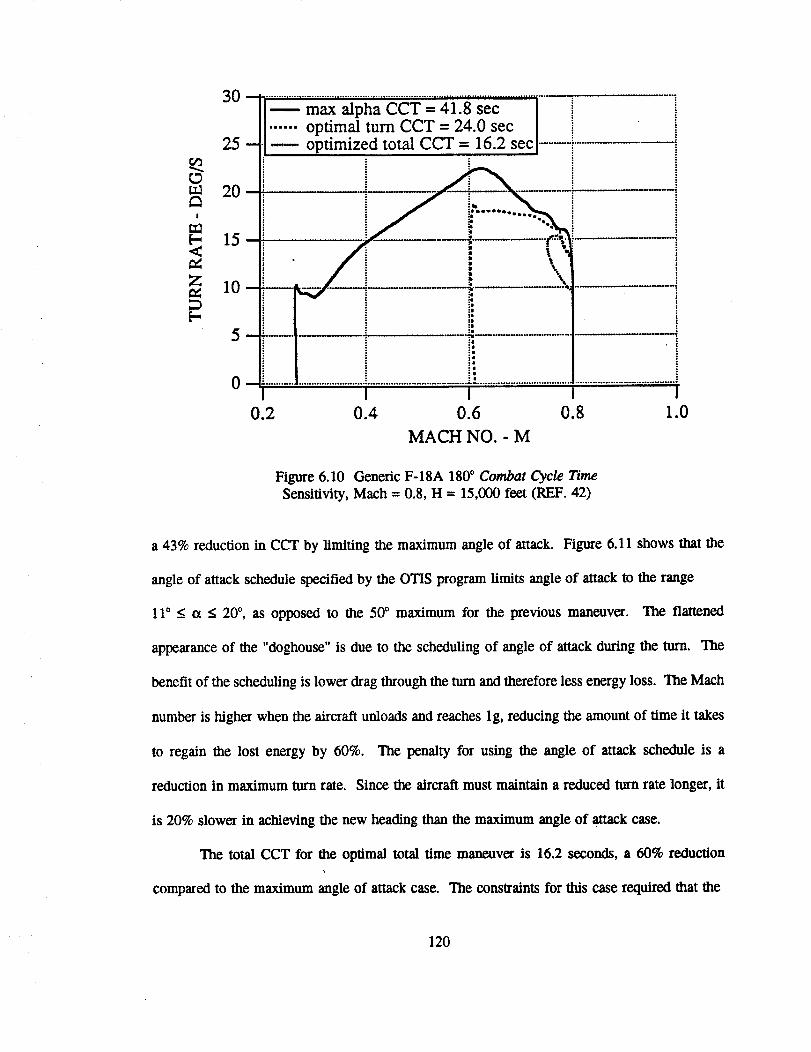
r_

!

[-<

[-

30-

25-

20-

15-

10-

m

.................................................................................. _o..oT ..............

-- max alpha CCT = 41.8 sec

...... optimal turn CCT = 24.0 sec

---- optimized total CCT = 16.2 sec

I

; i:a

:e

:l_a_°:l

I i

0.4 0.6 0.8 1.0

MACH NO. - M

Figure 6.10 Generic F-18A 180 ° Combat Cycle Time

Sensitivity, Mach = 0.8, H = 15,000 feet (REF. 42)

a 43% reduction in CCT by limiting the maximum angle of attack. Figure 6.11 shows that the

angle of attack schedule specified by the OTIS program limits angle of attack to the range

11° __.o_ < 20 °, as opposed to the 50 ° maximum for the previous maneuver. The flattened

appearance of the "doghouse" is clue to the scheduling of angle of attack during the turn. The

benefit of the scheduling is lower drag through the turn and therefore less energy loss. The Mach

number is higher when the aircraft unloads and reaches lg, reducing the amount of time it takes

to regain the lost energy by 60%. The penalty for using the angle of attack schedule is a

reduction in maximum turn rate. Since the aircraft must maintain a reduced turn rate longer, it

is 20% slower in achieving the new heading than the maximum angle of attack case.

The total CCT for the optimal total time maneuver is 16.2 seconds, a 60% reduction

compared to the maximum angle of attack case. The constraints for this case required that the

120

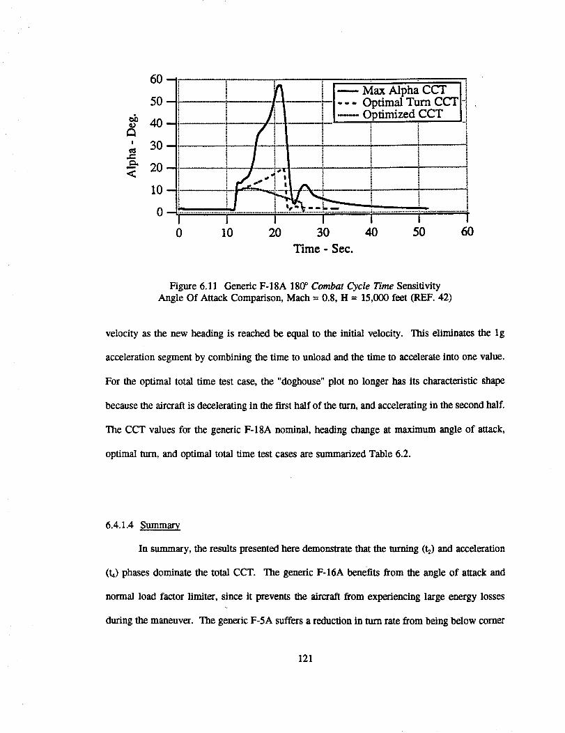
60-

50-

_4o_' 30

•-_ 20<

10

m

i _ I--- M.x_pha CCr i". [-_ _-1 _ Optimal Turn CC"Th ,

_/i._l__._i_|-__--s___._ : : ;

I I i I I

0 10 20 30 40 50 60

Time - Sec.

Figure 6.11 Genetic F-18A 180 ° Combat Cycle Time SensitivityAngle Of Attack Comparison, Mach = 0.8, H = 15,000 feet (P,EF. 42)

velocity as the new heading is reached be equal to the initial velocity. This eliminates the lg

acceleration segment by combining the time to unload and the time to accelerate into one value.

For the optimal total time test case, the "doghouse" plot no longer has its characteristic shape

because the aircraft is decelerating in the first half of the turn, and accelerating in the second half.

The CCT values for the generic F-18A nominal, heading change at maximum angle of attack,

optimal turn, and optimal total time test cases are summarized Table 6.2.

6.4.1.4 Summary

In summary, the results presented here demonstrate that the turning (h) and acceleration

(h) phases dominate the total CCT. The generic F-16A benefits from the angle of attack and

normal load factor limiter, since it prevents the aircraft from experiencing large energy losses

during the maneuver. The generic F-5A suffers a reduction in turn rate from being below corner

121

Table6.2 Generic F-18A 180 ° Combat Cycle Time

Sensitivity Results, Mach= 0.8, H = 15,000 feet

test case Combat Cycle Time (see)

nominal 43.7

maximum angle of attack 41.8

optimal turn 24.

optimal total CCT 16.2

speed at the test Mach number. Had the initial Mach number been higher, the generic F-SA

would probably have performed better. Consequently, a lower initial Mach number would

probably result in a worse performance. These considerations demonstrate that comer speed has

a strong influence on the outcome of the CCT, and should be kept firmly in mind when evaluating

results obtained using this metric. At the start of the acceleration phase, both the generic F-18A

and generic X-29A suffer from severe energy losses. This is largely due to the pilot command

input strategy used for testing these aircraft, since angle of attack is permitted to (unrealistically)

exceed that for maximum lift. Thus, the generic F-18A and generic X-29A are forced to perform

at a disadvantage.

These results support the hypothesis in Reference 1 that the CCT metric is dominated by

sustained capabilities such as turn rate and level acceleration. These capabilities are in turn

dependent upon the traditional measures of merit of wing loading and thrust-to-weight ratio.

Although it does not quanti_ transient agility, the CCT metric is useful in that it: i) provides a

122

measureof theabilityof anaircrafttotransitionbetweensustained maneuver states and ii) stresses

the importance of minimizing the time required to point the nose while keeping the significant

energy losses associated with hard nose pointing maneuvers to a minimum.

The cur metric is highly sensitive to the particular type of maneuver (nominal, maximum

angle of attack, optimal turn, optimal total time) used to test it. The maneuver is dictated by the

angle of attack schedule which is followed, which significantly affects measured values of the

metric. Additionally, which maneuver is best from an operational standpoint is highly dependent

on the combat situation. For example, from the context of operations the turn segment might

likely involve a pitch up to bleed airspeed, followed by a descending slice back for gravity assist

to help tighten the turn (REF. 52). Naturally, this technique might also vary somewhat according

to the aircraft being flown.

Therefore when drawing conclusions, the combat utility of all three types of maneuvers

must be carefully weighed against the particular objective or task the pilot is trying to accomplish.

This also underscores the need to standardize test procedures in agility flight testing. If the

optimal maneuvers had been used, the generic F-5A and generic F-18A would compare more

favorably to the other aircraft since they would not have been forced into large energy loss

situations.

6.4.2 Combat Cycle Time 90* Heading Change (REF. 30)

6.4.2.1 Definition

This metric is defined as the sum of: t_ + t21 + h2 + t3 + t4

where tl = time to pitch from one g to the limit normal load factor

123

t21 + 1,22

t3

t4

= time to turn to a specified new heading angle at maximum normal loadfactor

= time to unload to a normal load factor of either one or zero g

= time to accelerate to the original energy level

6.4.2.2 Discussion and Typical Results

This metric is completely analogous to the 1800 CCT of Section 6.4.1, except that the

specified new heading angle is 90 degrees. Results for the generic X-29A are not presented for

the 90 ° CCT since the simulator was not available at the time the investigation was being

conducted. The 90 ° CCT plot for the generic F-5A is shown in Figure 6.12. The 90 o CCT for

this aircraft is very similar to the results for the 180 ° CCT, in that all of the maneuvering occurs

along the normal load factor limit line. This is because the 90 degree heading angle is captured

before comer speed is reached.

Figure 6.13 shows the 90 ° CCT plot for the generic F-16A. Like the generic F-5A, this

aircraft also maneuvers only along its normal load factor limit line, since the 90 degree heading

angle is captured before comer speed is reached. The segment h2 is not applicable for the generic

F-16A when performing the 90 ° CCT.

Figure 6.14 shows the 90 ° CCT plot for the generic F-18A. Like the generic F-5A and

generic F-16A, the generic F-18A is seen to maneuver only along its normal load factor limit line

for the same reason.

6.4.2.3 Combat Cycle Time 90 ° Heading Change Sensitivity

The sensitivity analysis for the 90 ° CCT metric is performed using the angle of attack

schedules specified by the OTIS program. Because of the short time scale involved with the 900

124

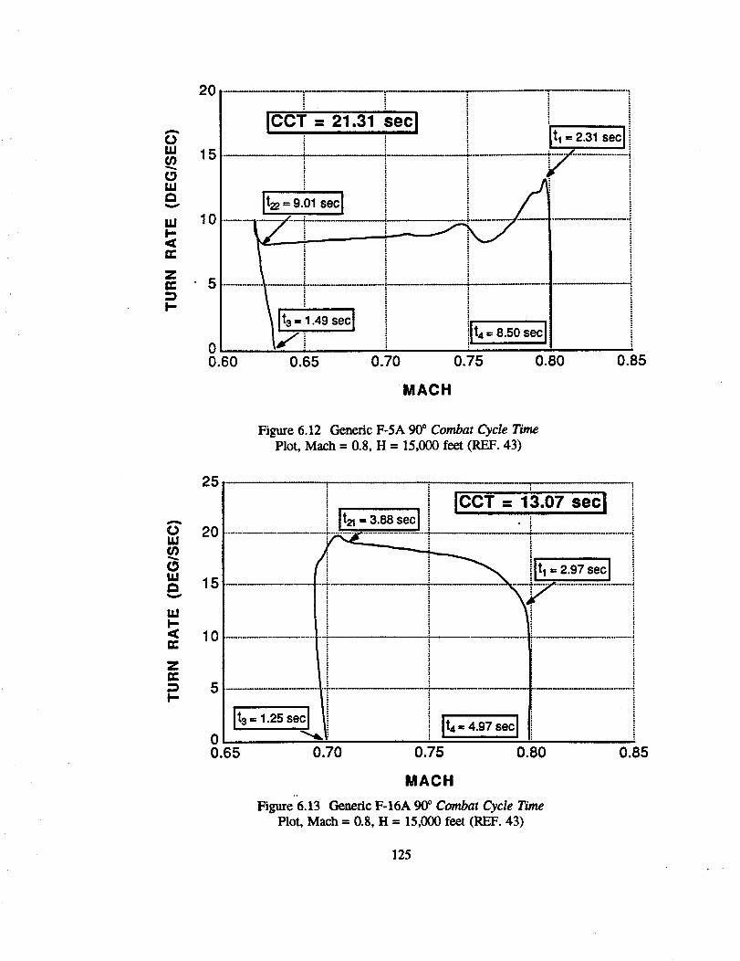
20

A

OI¢1O3OIJ.I

I¢1I.-,,¢n..

Z

I-

15

10

5

00.60

ICCT = 21.31 sec I

i

0.70

It22= 9.01 secI

.......... ii

.49 sec I

0.65

AI,

It,--_,secI

J

0.85

MACH

Figure 6.12 Genedc F-5A 90 ° Combat Cycle TimeP10t, Mach= 0.8, H = 15,000 feet (REF. 43)

25

A

O=11O3

OIJJt_

UJI-

Ztr"

!-

20

15

10

5

0

! . iccT= 13.07s,cli It_ 3SssecI .:;

t3 = 1.25 sec It4 = 4.97 sec I

0.65 0.70 0.75 0.80

MACH

Figure 6.13 Generic F-I6A 90 ° Combat Cycle Time

Plot, Mach= 0.8, H = 15,000 feet (REF. 43)

0.85

125

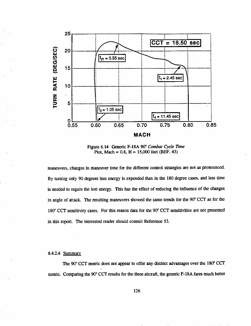
25

A

0 20I.Uo')¢3I,,1.1a 15

wI,.-< 10n-,

zn..:_ 5I..-

0

isecl

It I = 2.45 sec Ii

]

i

t4= 11.45 sec I

0.55 0.60 0.65 0.70 0.75 0.80 0.85

MACH

Figure 6.14 Generic F-18A 90 ° Combat Cycle TimePlot, Math = 0.8, H = 15,000 feet (REF. 43)

maneuvers, changes in maneuver time for the different control strategies are not as pronounced.

By turning only 90 degrees less energy is expended than in the 180 degree cases, and less time

is needed to regain the lost energy. This has the effect of reducing the influence of the changes

in angle of attack. The resulting maneuvers showed the same trends for the 90 ° CCT as for the

180 ° CCT sensitivity cases. For this reason data for the 90 ° CCT sensitivities are not presented

in this report. The interested reader should consult Reference 53.

6.4.2.4

metric.

Summary

The 90 ° CCT metric does not appear to offer any distinct advantages over the 180 ° CCT

Comparing the 90 ° CCT results for the three aircraft, the generic F-18A fares much better

126

against the generic F-16A and F-5A for the 90 degree heading angle change because it is not

commanded to as high an angle of attack as it was for the 180 degree case, thereby avoiding high

energy bleed rates. The overall 90 ° CCT performance of the generic F-5A once again suffers

because of its reduced turn rate capability, as it requires roughly twice as long as the other aircraft

to complete the 90° turn.

6.4.3 Dynamic Speed Turn (REF. 47, 54)

6.4.3.1 Definition

plot of Ps versus maximum turn rate at a given starting airspeed.

6.4.3.2 Discussion and Typical Results

The intent of the dynamic speed turn metric is to capture the dynamic maneuvering

capability of fighter aircraft (agility) as viewed from a pilots perspective, and to present that

capability in a form which can be readily used by pilots and engineers. Dynamic speed turn plots

show the dynamics of turning and acceleration over a wide range of speeds, combine the ability

of the aircraft to point its nose, continue pointing its nose, and accelerate. This is accomplished

by presenting information in the form of two distinct plots: one clearly showing the bleed rate for

maximum acceleration turns, and another showing the slraight and level acceleration capability

at various airspeeds.

The dynamic speed turn plots for the generic F-5A, F-16A, F-18A, and X-29A are derived

from the nominal 180 ° CCT maneuvers of Section 6.4.1. The generic F-5A dynamic speed turn

plots are shown in Figure 6.15. Maneuvering along the normal load factor and lift limit lines is

represented by Figure 6.15a, which plots turn rate versus bleed rate. The straight line acceleration

127

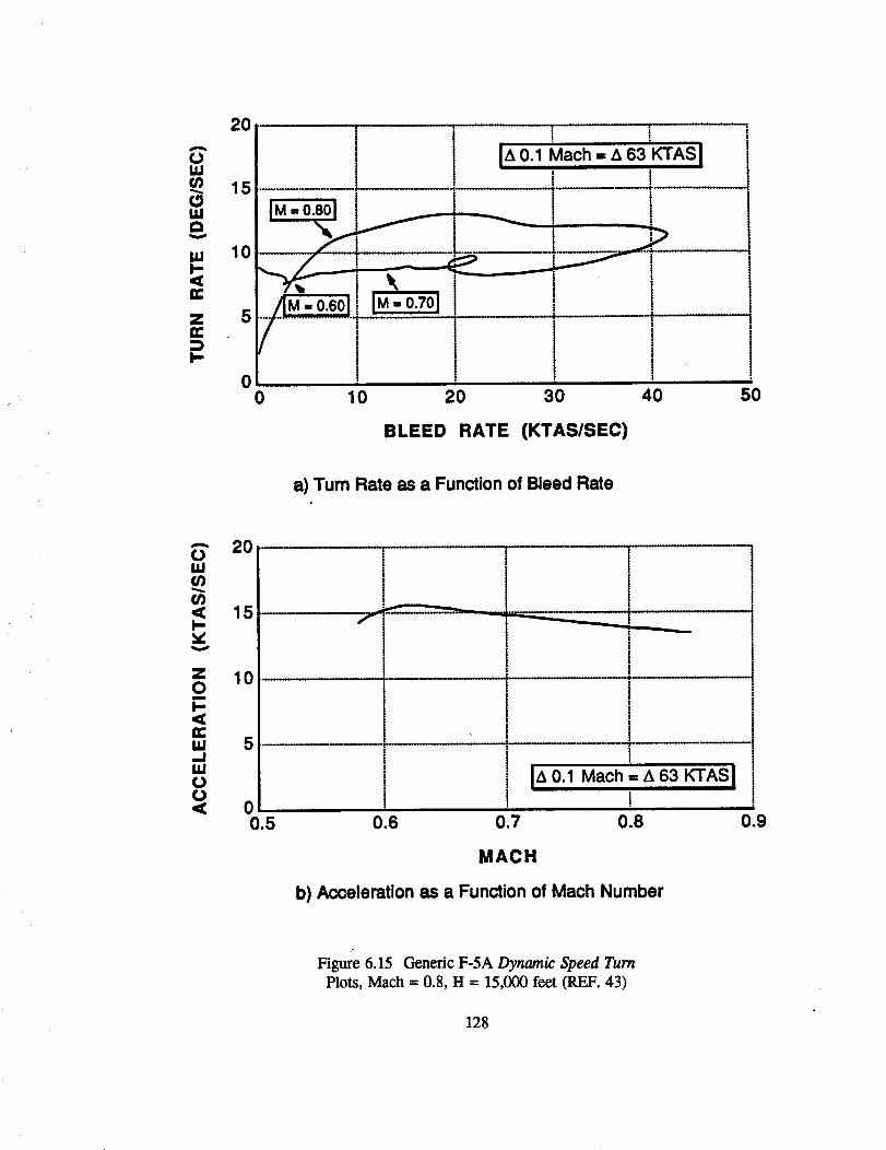
A

Ou,i03Ou,I

u.II.-,<=:

;[¢C

I-,.

20

15

10

5

0

IA 0.1 Mach = A 63 KTAS It {

nM-*o_

r I t { {0 0 20 30 40 50

BLEED RATE (KTAS/SEC)

a) Turn Rate as a Function of Bleed Rate

ou,i0303

I-

zOm

I-,c¢G:u.I_Ju,IOO

20

15

10

5

0

I{{

{{{!{

IA 0.1 Mach = A 63 KTASI!

0.5 0.6 0.7 0.8

MACH

b) Acceleration as a Function of Mach Number

0.9

Figure 6.15 Generic F-5A Dynamic Speed TurnPlots, Mach = 0.8, H = 15,000 feet (REF. 43)

128

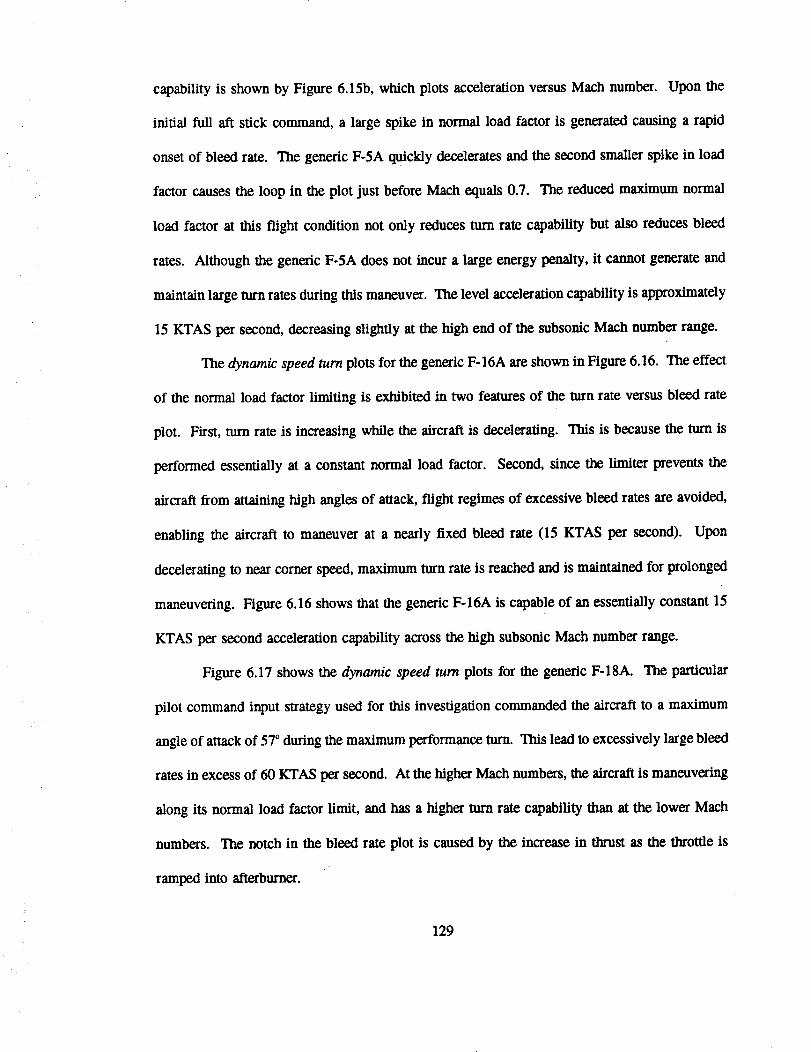
capability is shown by Figure 6.15b, which plots acceleration versus Mach number. Upon the

initial full aft stick command, a large spike in normal load factor is generated causing a rapid

onset of bleed rate. The generic F-5A quickly decelerates and the second smaller spike in load

factor causes the loop in the plot just before Mach equals 0.7. The reduced maximum normal

load factor at this flight condition not only reduces turn rate capability but also reduces bleed

rates. Although the generic F-5A does not incur a large energy penalty, it cannot generate and

maintain large turn rates during this maneuver. The level acceleration capability is approximately

15 KTAS per second, decreasing slightly at the high end of the subsonic Mach number range.

The dynamic speed turn plots for the generic F-16A are shown in Figure 6.16. The effect

of the normal load factor limiting is exhibited in two features of the turn rate versus bleed rate

plot. First, turn rate is increasing while the aircraft is decelerating. This is because the turn is

performed essentially at a constant normal load factor. Second, since the limiter prevents the

aircraft from attaining high angles of attack, flight regimes of excessive bleed rates are avoided,

enabling the aircraft to maneuver at a nearly fixed bleed rate (15 KTAS per second). Upon

decelerating to near corner speed, maximum turn rate is reached and is maintained for prolonged

maneuvering. Figure 6.16 shows that the generic F-16A is capable of an essentially constant 15

KTAS per second acceleration capability across the high subsonic Mach number range.

Figure 6.17 shows the dynamic speed turn plots for the generic F-18A. The particular

pilot command input strategy used for this investigation commanded the aircraft to a maximum

angle of attack of 570 during the maximum performance turn. This lead to excessively large bleed

rates in excess of 60 KTAS per second. At the higher Math numbers, the aircraft is maneuvering

along its normal load factor limit, and has a higher turn rate capability than at the lower Mach

numbers. The notch in the bleed rate plot is caused by the increase in thrust as the throttle is

ramped into afterburner.

129

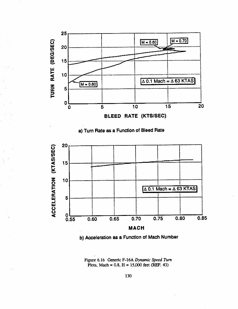
A

(JUJ

(3Illt_

U.II-,<=:

Zg:

I-

25

20

15

10

5

00

M-0.60 IM'0"_01

t I iI• i

BLEED RATE (KTS/SEC)

a) Turn Rate as a Function of Bleed Rate

A

U,I

<I-b¢

Z0m

I-,<IX:U.I__1U.I

O

20

15

10

5

i i

I I& 0.1 Mach = A 63 KTAS I1! i' t.

0 ' ! ;

0.55 0.60 0.65 0.70 0.75 0.60 0.85

MACH

b) Acceleration as a Function of Mach Number

Figure 6.16 C-enedc F-16A Dynamic Speed TurnPlots, Mach = 0.8, H = 15,000 feet (REF. 43)

130

25i I i !

IM-O,701 i _,,_ __t ........

II _ IM=O.S01i

I V I,-0.,011 i

IM- o.3o1 1 t 1

M- 0.80 [ IA 0.1 Mach = & 63 KTAS I

i i

10 ' 20 30 40 50 60 7'0

A

(JUJ(nf3uJD

I¢1I-,<=:

Z=::)I-,

2O

15

10

5

00

BLEED RATE (KTS/SEC)

a) Tum Rate as a Function of Bleed Rate

-- 20 .............OU,IU)(n<I-

Om

I-,<n-U,I_JU.IO(.1<

i i15

! • .

10 t

i. l, , i i

0 _ i i ,0.3 0.4 0.5 0.6 0.7 0.8 019

MACH

b) Acceleration as a Function of Mach Number

Figure 6.17 Generic F-18A Dynamic Speed Turn

Plots, Mach = 0.8, H = 15,000 feet (REF. 43)

131

ThegenericX-29A dynamic speed turn plots in Figure 6.18 highlight the difference

between the maneuver capability of that aircraft and the generic F-16A. Although both aircraft

have a flattened doghouse plot, the 30 KTAS per second bleed rate of the generic X-29A is nearly

twice that of the generic F-16A during the entire ann. This comparison demonstrates that the

generic X-29A may not be capable of achieving its maximum (theoretical) turn rate, whereas the

generic F-16A could do so were it not for the angle of attack and normal load factor Umiters. To

a large extent the inability of the generic X-29A to sustain a high normal load factor is due to the

higher angles of attack (and thus higher drag) attained by the generic X-29A during the turn, and

to a lesser extent by thrust-to-weight considerations (REF. 43). The generic X-29A level

acceleration capability is approximately 10 to 12 KTAS per second across the mid to high

subsonic Mach number range.

Perhaps the most useful feature of the dynamic speed turn plots is the ability to clearly

compare the maneuver capability of dissimilar aircraft. For the purpose of relative comparison

between the four aircraft, the respective dynamic speed turn plots are superimposed into a single

combined dynamic speed turn plot in Figure 6.19. The turn rate versus bleed rate plot shows that

an aircraft maneuvering in the region upwards and to the left side of the plot is desirable as this

indicates a high turn rate capability at low bleed rates. The generic F-16A appears to dominate

as it has a higher turnrate and lower bleed rate than either the generic F-5A, F-18A, or X-29A.

In terms of acceleration capability the generic F-5A and generic F-16A are comparable, exceeding

abe generic F-18A and generic X-29A by approximately 2 to 3 KTAS per second. Although the

X-29A exhibits lower bleed rates than the generic F-18A, its acceleration capability is several

KTAS per second less than the generic F-18A for the low subsonic Mach numbers. This results

in equivalent values for the CCT.

132

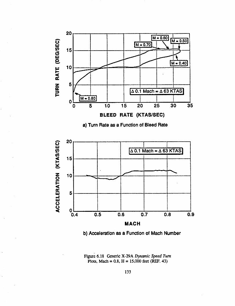
tOuJ¢n

Ou.ID

u.II,-

e_

ZOC

I.,-

2O

15

10

5

00

t

IM-O.SOI .,

5 10

! IM'.o6ol.i .• • i _,-" IM = 0.501

i ...... "................i........ '

I'!IA0.1i_ch=Aea_rASI

i t t! . !i i

15 20 25 30 35

BLEED RATE (KTAS/SEC)

a) Turn Rate as a Function of Bleed Rate

A 20

=9 lo

! . TI"o.1Mach A 63KTASI

m 5_Jwoo< 0

0.4

i ||

i t

!, !

st

" i i i

0.5 0.6 0.7 0.8 0.9

MACH

b) Acceleration as a Function of Mach Number

Figure 6.18 Genedc X-29A Dynamic Speed Turn

Plots, Mach= 0.8, H = 15,000 fe_t (REF. 43)

133

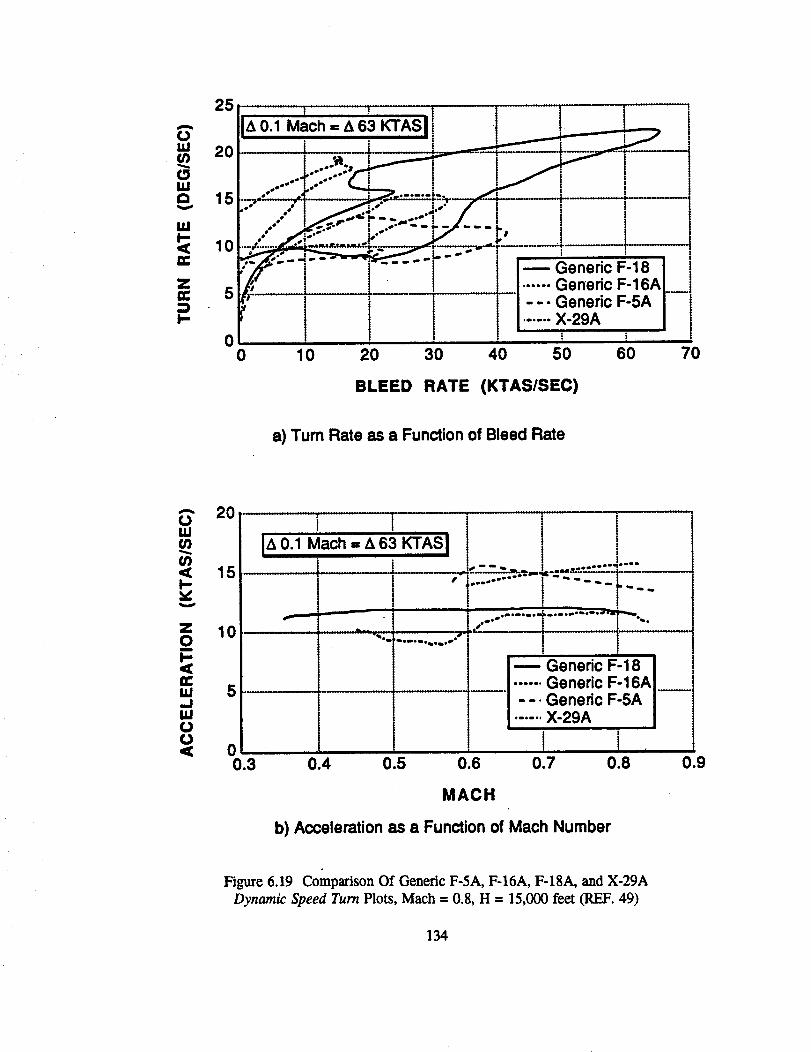
25

A

0W

Wa

WI-<

Z

p-

20

15

10

5

00

i :' I i I&0.1Mach=&63KTASlt -i I , -,

......t , .J

.,'- .,r" _ ...... f,.o _ 1 . .. |7---_.'r_."_i- i '- i

." __'"'-" _" "" " i', I i• o_ B_ ¥ .I/_t- I......-!---

_" _ j J j ._'eric F-16AL_ii" T T --- Generic F-5A I i

i i o n

10 20 30 40 50 60 70

BLEED RATE (KTAS/SEC)

a) Turn Rate as a Function of Bleed Rate

A

¢.)IJJ

¢n¢¢I-v

ZOm

WJW00

0 ,[, _ [ L,

i il& 0.1 Mach = & 63 KTAS I

i i15, ,L ,

!10 ..........

,,, ..... L,,

0

l f!

__o_eoe°m°_ e°°°

i .

_.Oeoe _'_lt.e

I !Generic F-18...... Generic F-16A

! --. Generic F-5AI ...... X-29Ai

"_°abl • 0_• e • -o _ iBoo •

!

0.3 0.4 0.5 0.6 0.7 0.8 0.9

MACH

b) Acceleration as a Function of Mach Number

Figure 6.19 Comparison Of Generic F-5A, F-16A, F-18A, and X-29A

Dynamic Speed Turn Plots, Mach= 0.8, H = 15,000 feet (REF. 49)

134

6.4.3.3Dynamic Speed Turn Sensitivity

The sensitivity of the dynamic speed turn metric to pilot command input strategy is

determined using the generic F-18A and the OTIS program. Figure 6.20 shows the generic F-18A

dynamic speed turn plots for the three cases of heading change at maximum angle of attack CCT,

optimal total turn CCT, and optimized total CCT. The data in Figure 6.20 is generated by the

generic F-18A simulation using the angle of attack schedules specified by the OTIS program for

the 180 ° CCT.

Considering the turn rate versus bleed rate plot first, the desirable test case is defined here

as the one which results in minimal bleed rates but still allows a high turn rate. Tiffs produces

a good combination of low maneuver time and low energy loss. The maximum angle of attack

CCT test case demonslrates the consequence of maneuvering at high angle of attack. The bleed

rates are in excess of 60 KTAS per second during the maneuver, since the aircraft decelerates

from Mach equals 0.8 to Mach equals 0.25. It is evident from Figure 6.20 that the optimal turn

CCT test case achieves a high value of turn rate, yet produces a lower bleed rate than the

maximum angle of attack CCT test case. The optimal total CCT test case reduces bleed rates

even further, but does not achieve maximum turn rate until the end of the maneuver. The fiat

appearance of the slope is due to the scale used to plot the graph. The energy efficiency is

evidenced by the very small loss of airspeed during the turning portion of the maneuver. The

optimal total CCT test case also shows that the maximum bleed rate for this maneuver is only 12

KTAS per second, compared to the 60 KTAS per second for the maximum angle of attack CCT

test case. The optimal total CCT test case and the optimal turn CCT test case both show that by

performing the maneuver at lower angles of attack, the maximum bleed rate is approximately 20

KTAS per second, compared to the 60 KTAS per second for the maximum angle of attack CCT

test case.

135

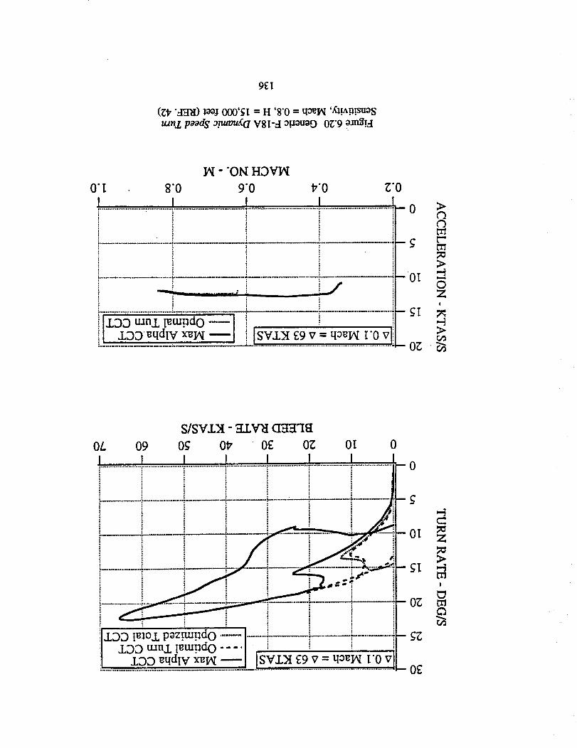
9gI

(_, "_) _ 000'_I = H '8"0 = q_I_I '_!a._isuoS_nz p_d S o_.uamK.(lV81-4 o.uouoo OU9 o.m_!.4

IAI - "ON HDVIAI

9"0O'I 80 ¢'0 Z'O

........................_............................................................................................................ I O

/-- I II ...... -"

[JL.DD tunA, [gtu!ld 0 .... [ I[ _LDD _qdlV x_N _ SVZN E9 v = qo_IAI I'Ov

-Ol

-_I

- O_

>

7=>

0ZI

>

S/S'v'J2,I - _LV_I CICEr-J"l_I

OL 09 Og Olr Og OZ OI 0

SVZXA E9 v = qo_I_I['0v

0

>

!

OZ rnc_

OE

The acceleration versus Mach number plot in Figure 6.20 for the maximum angle of attack

CCT test case shows that the generic F-18A is capable of a straight and level aczelerafion of 12

KTAS per second, or a sustained acceleration of approximately 0.6 g. This information is useful

for estimating how long it will take the pilot to regain lost energy at a given flight condition. The

optimal turn CCT test case shows that the generic F-18A accelerates straight and level at about

12 KTAS per second for this maneuver. This test case matches the plot for the maximum angle

of attack CCT test case since the generic F-18A is at full throttle, indicating that the maximum

straight and level acceleration for the generic F-18A at 15,000 ft is approximately 12 KTAS per

second. The optimal total CCT test case shows the generic F-18A to be accelerating at its

maximum capability of approximately 12 KTAS per second for this test case, which is again

virtually identical to the other two test cases. It is interesting to note that this angle of attack

schedule results in a maximum bleed rate of 12 KTAS per second, which is equal to the maximum

level acceleration of the aircraft=

In terms of the dynamic speed turn metric, the 180 ° optimal total CCT is judged to be the

best command input strategy. This is in spite of the fact that the optimal total CCT test case is

actually slower in reaching the final heading angle.

A similar dynamic speed turn analysis using the 90 ° cur cases (REF. 53) showed that

the maneuver time is too small to allow the bleed rate to increase to a significant level. The turn

rate versus bleed rate plots for these maneuvers are not included since they are almost identical

to Figure 6.20. The acceleration of the aircraft is not changed appreciably from the previous test

cases, and the different control strategies do not yield significant changes in the shape of the plots.

137

6.4.3.4 Summary

The dynamic speed turn metric provides useful information regarding

capabilities. The two plots relate maneuverability to three combat relevant tasks:

maneuver

.

2.

.

The ability to point the nose of the aircraft

The ability to continue pointing the aircraft quickly, i.e. residualturn rate.

The capability to disengage or regain speed.

As indicated in Section 6.4.3.3, the generic F-18A and generic X-29A incur large energy losses

during the 180 ° turn reversal because they are commanded to maneuver at high angles of attack.

These high angles of attack are a direct result of the pilot command input strategy used. The

generic F-16A is able to avoid incurring large energy losses with the same basic pilot command

input strategy because of its angle of attack limiter. However, this same angle of attack limiter

also res_icts the maximum maneuver potential of the generic F-16A. In limiting the maximum

angle of attack for this maneuver, a trade-off occurs between energy preservation 0ower bleed

rates) versus the effectiveness of high angle of attack maneuvering (rapid heading angle changes).

Another consideration is that these maneuvers generate significant downrange and crossrange

distances, which could be significant.

The pilot command input strategy to use for the best dynamic speed turn results is defined

as that which results in the maximum angle of attack for which increasing turn rates at the

expense of increased bleed rates results in diminshing returns (REF. 47). Performing the dynamic

speed turn at this angle of attack maximizes maneuver potential while minimizing energy losses.

The sensitivity analysis for this metric shows that the 1800 optimal total CCT test case produces

the angle of attack schedule for the best dynamic speed turn performance.

138

6.4.4 Relative Energy State (V/V_) (RF_. 30)

6.4.4.1 Definition

The ratio of the aircraft's speed to its comer speed at the completion of a 180 ° turn at

maximum normal load factor from a given starting position (altitude and airspeed). This

ratio, VNc, should be as close to 1.0 as possible.

6.4.4.2 Discussion and Typical Results

The relative energy state metric is intended to quantify the capability of an aircraft

engaged in WVR air combat to execute multiple 90 degree turns. The presentation of this metric

consists of plots of the ratio of aircraft speed to comer speed for various heading angle changes.

In testing the relative energy state metric, the number of 90 degree turns an aircraft is required

to execute is not specified by the definition of the metric. However, the author of this metric

suggests in Reference 30 that at least two 90 degree turns be completed before the speed of the

aircraft falls below corner speed. When an aircraft is flying below corner speed, it has in essence

maximized pointing capability, while exhausting maneuvering potential. Conversely, when flying

above comer speed, an aircraft retains energy for future maneuvering while sacrificing maximum

pointing capability (REF. 49).

Data for the relative energy state metric is obtained directly from the 180 ° CCT maneuver

of Section 6.4.1. The relative energy state for the generic F-5A, generic F-16A, generic F-18A,

and generic X-29A is plotted versus heading angle in Figure 6.21. From Figure 6.21 it is seen

that the generic F-18A loses speed during the turn reaching a relative energy state of 0.62 at 180 °,

whereas the generic F-16A is seen to maintain its speed relatively well with a final relative energy

state of 0.92. The X-29A loses airspeed at a constant rate throughout the heading change with

the relative energy state remaining above 1.0 for the first 900 turn, and then reaching a value of

0.70 by the end of the second turn.

139

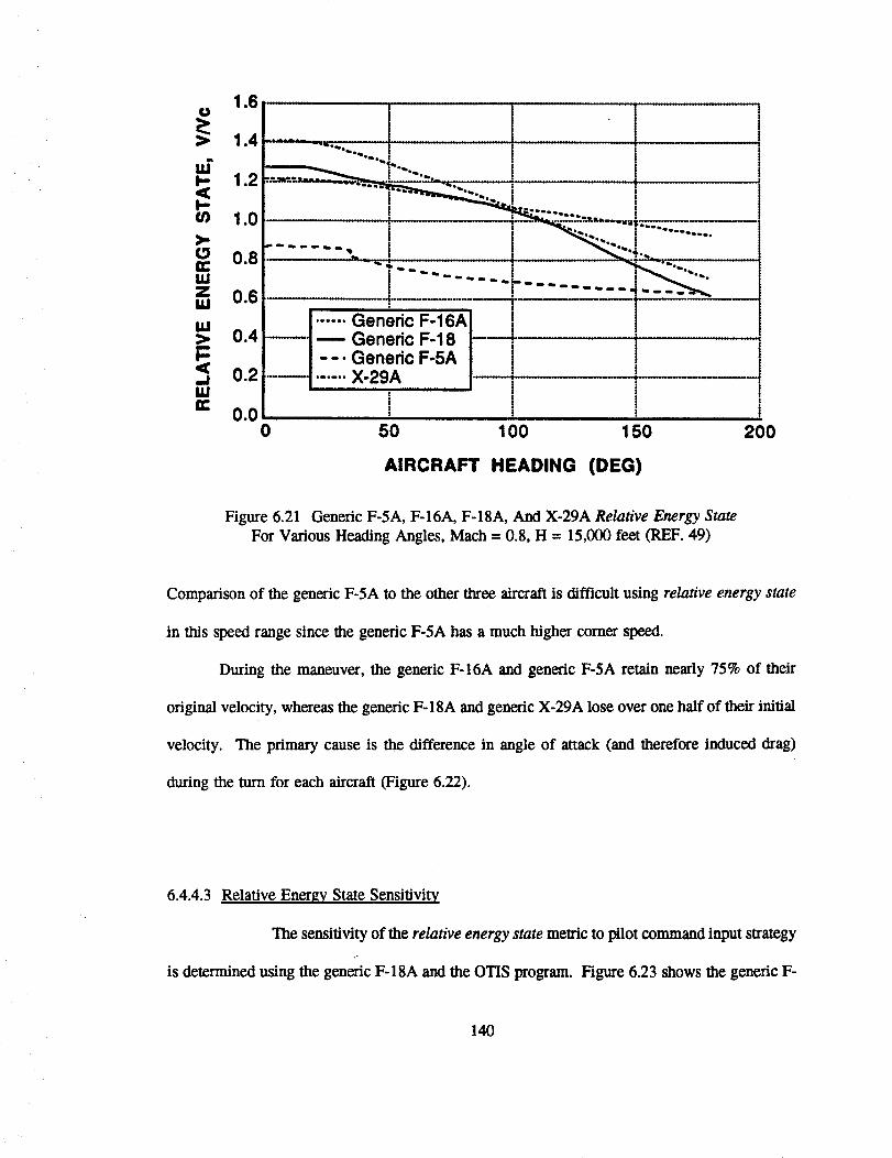
1.6o

1.4

tu"v,- 1.2,<I-u_ 1.0>-¢.-1 0.8

U.Iz 0.6I,IJ

U.I> 0.4I-< 0.2,.II¢1=¢

0.0

_.ll,._o_ ' ,, , ,tL ,, .......................

l _"',---. ..... __

" .... i .... '"" .... -

.... " "_,. I , _ Z/"_..

i

°ncF.Genedc F-18Genedc F-5AX-29A

!

!

!¢

i ,!

0 50 100 150

AIRCRAFT HEADING (DEG)

I

200

Figure 6.21 Generic F-5A, F-16A, F-18A, And X-29A Relative Energy State

For Various Heading Angles, Mach= 0.8, H = 15,000 feet (REF. 49)

Comparison of the generic F-5A to the other three aircraft is difficult using relative energy state

in this speed range since the generic F-5A has a much higher comer speed.

During the maneuver, the generic F-16A and generic F-5A retain nearly 75% of their

original velocity, whereas the generic F-18A and generic X-29A lose over one half of their initial

velocity. The primary cause is the difference in angle of attack (and therefore induced drag)

during the turn for each aircraft (Figure 6.22).

6.4.4.3 Relative Energy State Sensitivity

The sensitivity of the relative energy state metric to pilot command input strategy

is determined using the generic F-18A and the OTIS program. Figure 6.23 shows the generic F-

140

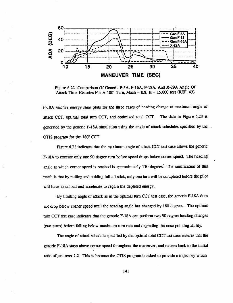
60A

OWO

<0<

40

20

010

! .... "-_'_'_! t.... I.--G_enF-SA I-----+.I ./! .... ,\ { ! I_GenF-IBI iT.... .._""-'+3' .... +.+X.... "-1 +........I ..... Gen F-lSAI ...... i

...................... f'"/_ ...... :_'_'......."i".................... " ......] ..... X-29A I.........

.... J,.$* • " .m.m_...m,.m.m.m.m_.w.AL.m.m. --....._ ..... "

p-__..=. -'- 1 " -,._ i,'-- ", i I t ,.........__.: ..................,......l..........................!: • • : -'p ....... , ! __ :......... ........ .... .-,

15 20 25 30 35 40

MANEUVER TIME (SEC)

Figure 6.22 Comparison Of Generic F-5A, F-16A, F-18A, And X-29A Angle OfAttack Time Histories For A 180 ° Turn, Mach= 0.8, H = 15,000 feet (REF. 43)

F-18A relative energy state plots for the three cases of heading change at maximum angle of

attack CCT, optimal total turn CCT, and optimized total CCT. The data in Figure 6.23 is

generated by the generic F-18A simulation using the angle of attack schedules specified by the

OTIS program for the 180 ° CCT.

Figure 6.23 indicates that the maximum angle of attack CCT test case allows the generic

F-18A to execute only one 90 degree turn before speed drops below comer speed. The heading

angle at which comer speed is reached is approximately 110 degrees" The ramification of this

result is that by pulling and holding full aft stick, only one turn will be completed before the pilot

will have to unload and accelerate to regain the depleted energy.

By limiting angle of attack as in the optimal turn CCT test case, the generic F-18A does

not drop below comer speed until the heading angle has changed by 180 degrees. The optimal

tam CCT test case indicates that the generic F-18A can perform two 90 degree beading changes

(two turns) before falling below maximum turn rate and degrading the nose pointing ability.

The angle of attack schedule specified by the optimal total CCT test case ensures that the

generic F-18A stays above comer speed throughout the maneuver, and returns back to the initial

ratio of just over 1.2. This is because the OTIS program is asked to provide a trajectory which

141

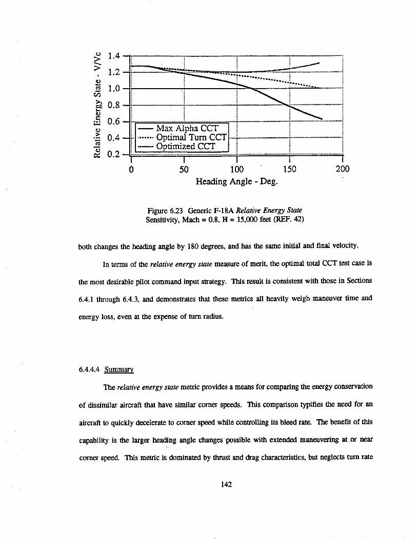
1.4

;> 1.2I

_ 10-

0.8-

e-ra 0.6-

•-> 0.4-

0.2-

0

; Q°I°Q .IOeQiIQ a i

ii i i .................

Max Alpha CCT

....... Optimal Turn CCT_n. Optimized CCT i

I I I

50 100 150 200

Heading Angle - Deg.

Figure 6.23 Generic F-18A Relative Energy State

Sensitivity, Math = 0.8, H = 15,000 feet (REF. 42)

both changes the heading angle by 180 degrees, and has the same initial and final velocity.

In terms of the relative energy state measure of merit, the optimal total CCT test case is

the most desirable pilot command input slrategy. This result is consistent with those in Sections

6.4.1 through 6.4.3, and demonstrates that these metrics all heavily weigh maneuver time and

energy loss, even at the expense of turn radius.

6.4.4.4 Summary

The relative energy state metric provides a means for comparing the energy conservation

of dissimilar aircraft that have similar comer speeds. This comparison typifies the need for an

aircraft to quickly decelerate to comer speed while controlling its bleed rate. The benefit of this

capability is the larger heading angle changes possible with extended maneuvering at or near

comer speed. This metric is dominated by thrust and drag characteristics, but neglects turn rate

142

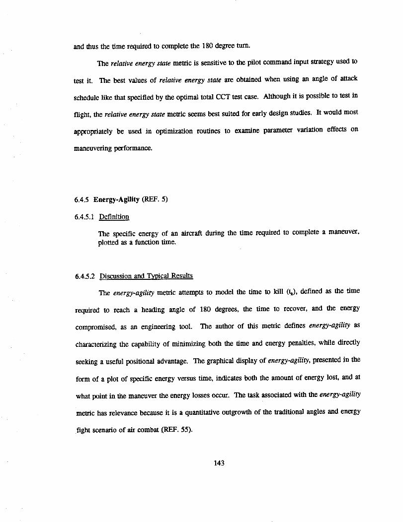
and thus the time required to complete the 180 degree turn.

The relative energy state metric is sensitive to the pilot command input strategy used to

test it. The best values of relative energy state are obtained when using an angle of attack

schedule like that specified by the optimal total CCT test case. Although it is possible to test in

flight, the relative energy state metric seems best suited for early design studies. It would most

appropriately be used in optimization routines to examine parameter variation effects on

maneuvering performance.

6.4.5 Energy-Agility (REF. 5)

6.4.5.1 Definition

The specific energy of an aircraft during the time required to complete a maneuver,

plotted as a function time.

6.4.5.2 Discussion and Typical Results

The energy-agility metric attempts to model the time to kill (tt), defined as the time

required to reach a heading angle of 180 degrees, the time to recover, and the energy

compromised, as an engineering tool. The author of this metric defines energy-agility as

characterizing the capability of minimizing both the time and energy penalties, while directly

seeking a useful positional advantage. The graphical display of energy-agility, presented in the

form of a plot of specific energy versus time, indicates both the amount of energy lost, and at

what point in the maneuver the energy losses occur. The task associated with the energy-agility

metric has relevance because it is a quantitative outgrowth of the traditional angles and energy

fight scenario of air combat ICREF. 55).

143

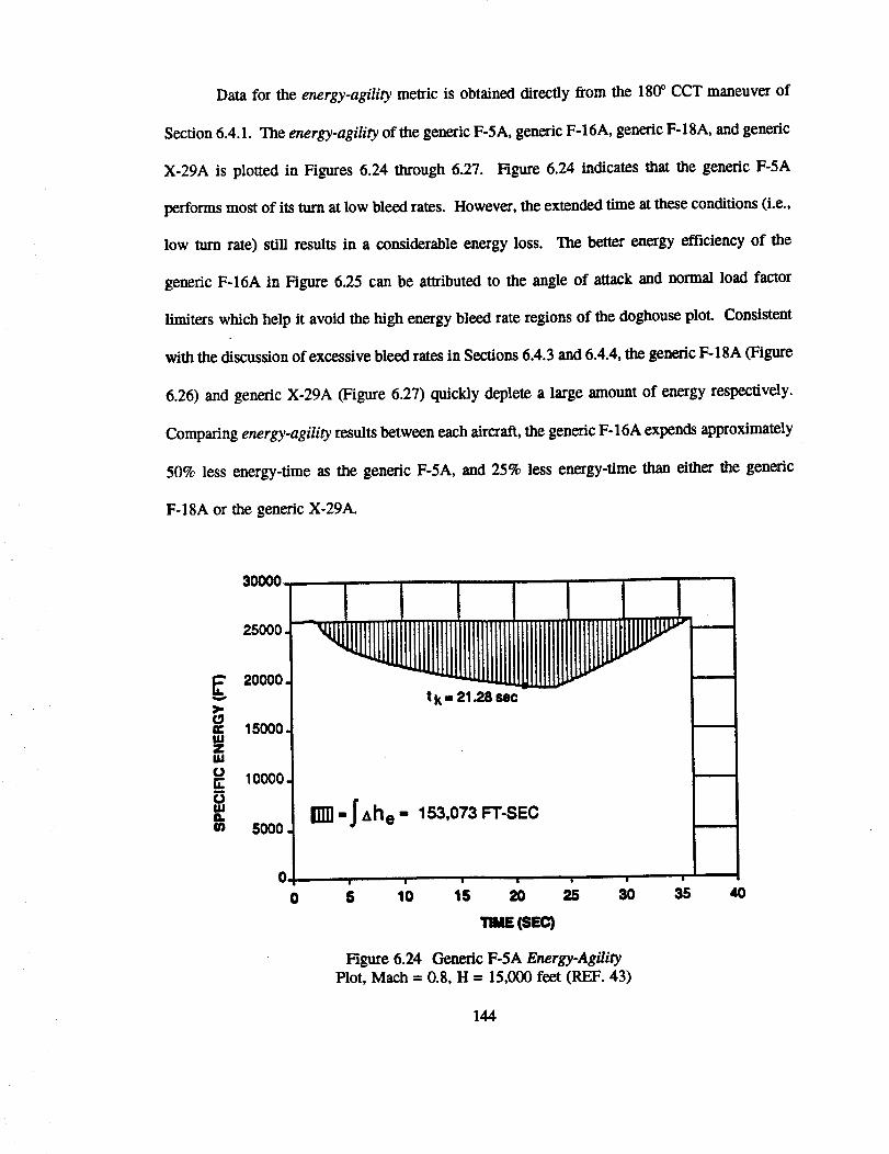
Datafor the energy-agility metric is obtained directly from the 180 ° CCT maneuver of

Section 6.4.1. The energy-agility of the generic F-5A, generic F-16A, generic F-18A, and generic

X-29A is plotted in Figures 6.24 through 6.27. Figure 6.24 indicates that the generic F-5A

performs most of its turn at low bleed rates. However, the extended time at these conditiom (i.e.,

low turn rate) still results in a considerable energy loss. The better energy efficiency of the

generic F-16A in Figure 6.25 can be attributed to the angle of attack and normal load factor

limiters which help it avoid the high energy bleed rate regions of the doghouse plot. Consistent

with the discussion of excessive bleed rates in Sections 6.4.3 and 6.4.4, the generic F-18A (Figure

6.26) and generic X-29A (Figure 6.27) quickly deplete a large mount of energy respectively.

Comparing energy-agility results between each aircraft, the generic F-16A expends approximately

50% less energy-time as the generic F-5A, and 25% less energy-time than either the generic

F-18A or the generic X-29A.

30000.

25000.

_ 20000

15000

i 10000.

5000.

0

I

t k" 21.28 sec

ITm-IAhe - 153,073 FT-SEC

5 10 15 2O 25 3O

11ME(st=c)

Figure 6.24 Generic F-SA Energy-AgilityPlot, Math = 0.8, H = 15,000 feet (REF. 43)

35

144

40

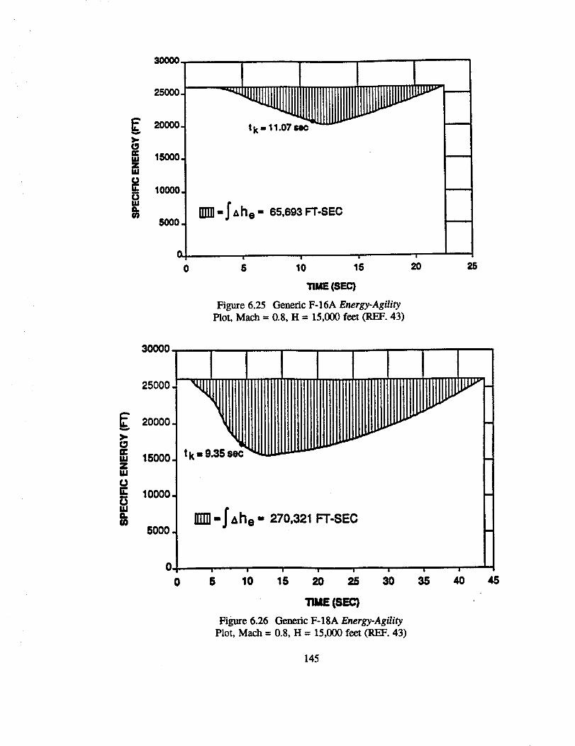
_)O01

25000.

20000.

15000.

..z,

10000.

t/)500O

tk- 11.07 sec

IT_ -J'_he - 65,693 FT-SEC

! | , I

0 5 10 15 20

TIME (SEC)

Figure 6.25 Genedc F-16A Energy-AgilityPlot, Mach = 0.8, H = 15,000 feet (REF. 43)

30000

OOOoooo15000 t

10000

FT SEC5000

0

0 5 10 15 20 25 30 35 40 45

I (SEC)

Figure 6.26 G-enefic F-18A Energy-Agility

Plot, Mach = 0.8, H : 15,000 feet (REF. 43)

145

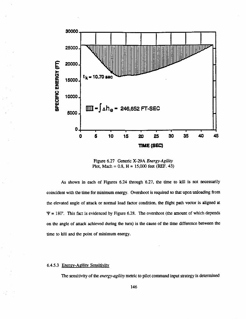
I • I20000. i

B

10000.

sooo SEC

0

0 5 10 15 2O 25 3O 35 4O 45

11ME(SF.C)

Figure 6.27 Generic X-29A Energy-AgilityPlot, Mach = 0.8, H = 15,000 feet (REF. 43)

As shown in each of Figures 6.24 through 6.27, the time to kill is not necessarily

coincident with the time for minimum energy. Overshoot is required so that upon unloading from

the elevated angle of attack or normal load factor condition, the flight path vector is aligned at

= 180 °. This fact is evidenced by Figure 6.28. The overshoot (the amount of which depends

on the angle of attack achieved during the turn) is the cause of the time difference between the

time to kill and the point of minimum energy.

6.4.5.3 Energy-Agility Sensitivity

The sensitivity of the energy-agility metric to pilot command input strategy is determined

146

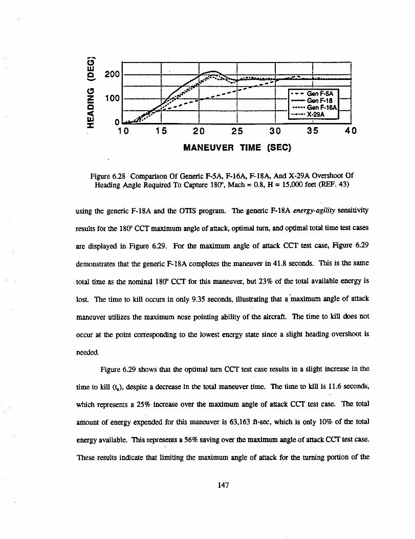
OIllH

OZm

H

tuX

200

100

0

l 0 ! .. i iL;4 * ....T - ." ,,.,_ ;-

! .f.f" J .----s"° i !---:_ I_";_i'-_----j;' T---I--'--"Gen F-18

_"i-- ! t 7-1......x:_A J--i10 15 20 25 30 35 40

MANEUVER TIME (SEC)

Figure 6.28 Comparison Of Generic F-5A, F-16A, F-18A, And X-29A Overshoot Of

Heading Angle Required To Capture 180 °, Mach= 0.8, H = 15,000 feet (REF. 43)

using the generic F-18A and the OTIS program. The generic F-18A energy-agility sensitivity

results for the 180 ° CCT maximum angle of attack, optimal turn, and optimal total time test cases

are displayed in Figure 6.29. For the maximum angle of attack CCT test case, Figure 6.29

demonstrates that the generic F-18A completes the maneuver in 41.8 seconds. This is the same

total time as the nominal 180 ° CCT for this maneuver, but 23% of the total available energy is

lost. The time to kill occurs in only 9.35 seconds, illustrating that a'maximum angle of attack

maneuver utilizes the maximum nose pointing ability of the aircraft. The time to kill does not

occur at the point corresponding to the lowest energy state since a slight heading overshoot is

needed.

Figure 6.29 shows that the optimal mrn CCT test case results in a slight increase in the

time to kill (t0, despite a decrease in the total maneuver time. The time to kill is 11.6 seconds,

which represents a 25% increase over the maximum angle of attack CCT test case. The total

amount of energy expended for this maneuver is 63,163 ft-sec, which is only 10% of the total

energy available. Tiffs represents a 56% saving over the maximum angle of attack CCT test ease.

These results indicate that limiting the maximum angle of attack for the turning portion of the

147

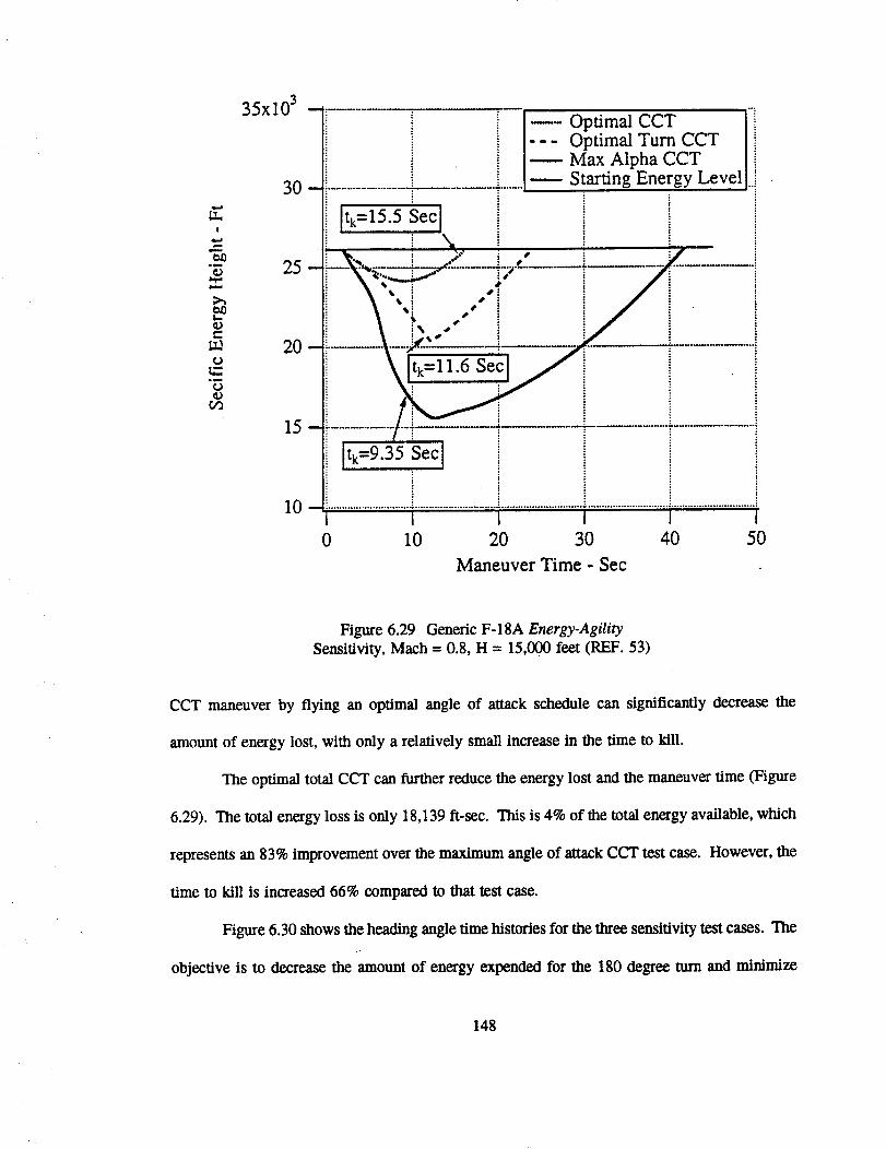
61b

!

e.,o,N¢D

e-

cDr_

35x103 --

30--

25--

20-

15-

10-

0

--.- Optimal CCT ii--- Optimal Turn CCT 1!----- Max Alpha CCT [i

Starting Energy Level].. i

[tk=15.5 Sec[ i

I ....i /

%: • i ! "_i ll' i i

_tk=l 1.6 Sec]_/

1tk-9.35 I

.............................. ; ............................. ._ ...........................................................................................

110 20 30 40 50

Maneuver Time - Sec

Figure 6.29 Generic F-18A Energy-Agility

Sensitivity, Mach = 0.8, H = 15,000 feet (REF. 53)

CCT maneuver by flying an optimal angle of attack schedule can significantly decrease the

amount of energy lost, with only a relatively small increase in the time to kill.

The optimal total CCT can further reduce the energy lost and the maneuver time (Figure

6.29). The total energy loss is only 18,139 ft-sec. This is 4% of the total energy available, which

represents an 83% improvement over the maximum angle of attack CCT test case. However, the

time to kill is increased 66% compared to that test case.

Figure 6.30 shows the heading angle time histories for the three sensitivity test cases. The

objective is to decrease the amount of energy expended for the 180 degree turn and minimize

148

!

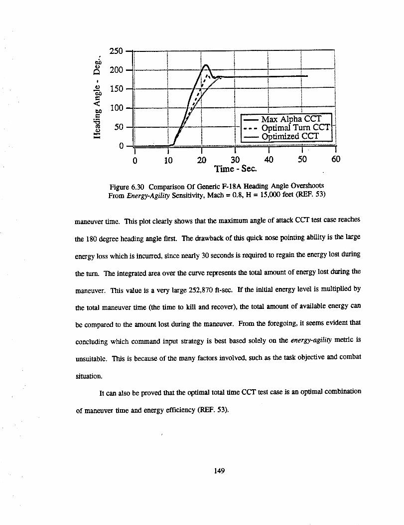
ued_

<

o_

t_

250 -

200 -

150 --

100 -

50-

0-

0

!.__ Max Alpha CCT [Optimal Turn CCT[- i

i Optimized CCT l i

I 'I I I I

10 20 30 40 50 60

Time - Scc.

Figure 6.30 Comparison Of Generic F-18A Heading Angle Overshoots

From Energy-Agility Sensitivity, Mach = 0.8, H = 15,000 feet (REF. 53)

maneuver time. This plot clearly shows that the maximum angle of attack CCT test case reaches

the 180 degree heading angle first. The drawback of this quick nose pointing ability is the large

energy loss which is incurred, since nearly 30 seconds is required to regain the energy lost during

the turn. The integrated area over the curve represents the totalamount of energy lost during the

maneuver. This value is a very large 252,870 ft-sec. If the initial energy level is multiplied by

the total maneuver time (the time to kill and recover), the total amount of available energy can

be compared to the amount lost during the maneuver. From the foregoing, it seems evident that

concluding which command input slrategy is best based solely on the energy-agility metric is

unsuitable. This is because of the many factors involved, such as the task objective and combat

situation.

It can also be proved that the optimal total time CCT test case is an optimal combination

of maneuver time and energy efficiency (REF. 53).

149

6.4.5.4 Summary

The energy-agility concept is a useful graphical technique to view the energy loss during

a combat relevant task. This metric is well suited to comparing the energy compromised during

the task by different aircraft, since each aircraft can be rated by its ability to minimize the energy

loss penalty while directly seeking a positional advantage. Determining the best pilot command

input strategy to use for testing the energy-agility metric is difficult because of the many inter-

related effects.

6.4.6 Time.Energy Penalty (REF. 43)

6.4.6.1 Definition

This metric is defined as

Time Energy Penalty = tar x h h e

where tax F is the time to complete a specified beading angle change and (if required) thetime to pitch down to achieve missile envelope firing parameters, and Ahe is the change

in specific energy height during the maneuver.

6.4.6.2 Discussion and Typical Results

The time tA_/consists of the sum of the time to roll 90 degrees and pitch to maximum

normal load factor (tl of combat cycle time), plus the time to obtain a specified heading angle (h

of combat cycle time), plus the time to pitch down and reduce angle of attack or normal load

factor so that an air-to-air missile can be fired within its envelope. The missile envelope is based

on the all-aspect AIM-9L Sidewinder which can be fired up to 25 degrees angle of attack and

approximately six to seven g (REF. 56). The change in specific energy height, Alae, is measured

150

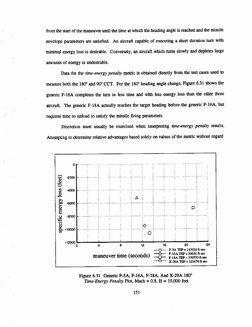
fromthestartof themaneuveruntil thetimeatwhichtheheadingangleisreachedandthemissile

envelopeparametersaresatisfied.

minimal energy loss is desirable.

amounts of energy is undesirable.

An aircraft capable of executing a short duration turn with

Conversely, an aircraft which turns slowly and depletes large

Data for the time-energy penalty metric is obtained directly from the test eases used to

measure both the 18& and 90 ° CCT. For the 180 ° heading angle change, Figure 6.31 shows the

generic F-16A completes the turn in less time and with less energy loss than the other three

aircraft. The generic F-18A actually reaches the target heading before the generic F-16A, but

requires time to unload to satisfy the missile firing parameters.

Discretion must usually be exercised when interpreting time-energy penalty results.

Attempting to determine relative advantages based solely on values of the metric without regard

_'_ -2000

-4000C)

m

-8000t_

_, -10000i<>

-12000 I 1 i I i I0 4 8 12

maneuver time (seconds)

O

i t

16i I i I

20 24

F-5A TEP= 143930 ft-_e

F-16A TEP = 59650 tl-_eF-18A TEP = 139550 R-_c

X-29A TI_ = 121670 It-see

Figure 6.31 Generic F-5A, F-16A, F-18A, And X-29A 1800

Time-Energy Penalty Plot, Mach= 0.8, H = 15,000 feet

151

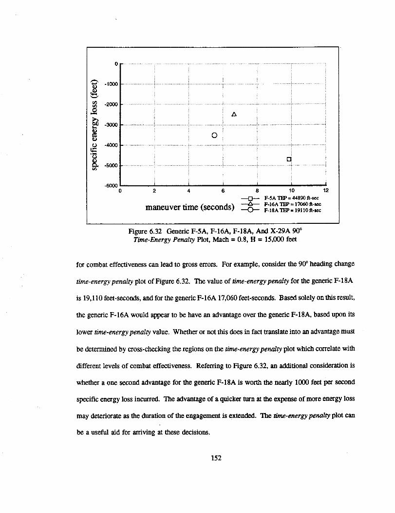
0 .................... ' ..................... ' ................................................................. _...................... "

C)

=o

Ct,

-lOOO

.2000

.3000

.4000

-5000

-6000o

A

C)

D_

I I I I I , I2 4 6 8 10 12

---D--- F-5A TI_ = 44890 _-se¢

_u)/SeCOn=S _ F-16A TEP = 17060 fi-mtimemaneuver --'O--- F-IgA TI_ = 19110t-race

Figure 6.32 Generic F-5A, F-16A, F-18A, And X-29A 90 °

Time-Energy Penalty Plot, Mach = 0.8, H = 15,000 feet

for combat effectiveness can lead to gross errors. For example, consider the 90° heading change

time-energy penalty plot of Figure 6.32. The value of time-energy penalty for the generic F-18A

is 19,110 feet-seconds, and for the generic F-16A 17,060 feet-seconds. Based solely on this result,

the generic F-16A would appear to be have an advantage over the generic F-18A, based upon its

lower time-energy penalty value. Whether or not this does in fact translate into an advantage must

be determined by cross-checking the regions on the time-energy penalty plot which correlate with

different levels of combat effectiveness. Referring to Figure 6.32, an additional consideration is

whether a one second advantage for the generic F-18A is worth the nearly 1000 feet per second

specific energy loss incurred. The advantage of a quicker turn at the expense of more energy loss

may deteriorate as the duration of the engagement is extended. "me time-energy penalty plot can

be a useful aid for arriving at these decisions.

152

6.4.6.3Time-Energy Penalty Sensitivity

The sensitivity of the time-energy penalty metric to pilot command input strategy is

determined using the generic F-18A simulation and the OTIS program. The data for the time-

energy penalty sensitivity study presented here is condensed from Reference 53. The generic F-

18A time-energy penalty sensitivity results for the 180* CCT maximum angle of attack, oplimal

turn, and optimal total time test cases are displayed in Figure 6.33. The desirable position on the

plot is to be as close to the origin as possible, or in the region of low energy loss and low

maneuver time. At a time-energy penalty of 135_.25.6 feet-seconds, the maximum angle of attack

CCT test case loses a considerable amount of energy compared to the optimal turn CCT test case,

which has a time-energy penalty of only 62,506 feet-seconds. Not unexpectedly, the optimal total

CCT test case reduces the time-energy penalty further still to 5,852.8 feet-seconds. According to

'_ -2000

-4000O

: 0oo

o -8000

_ -10000

X

nominal TI_ = 139550 R-see

max AOA TEP = 135225 ft-sec

optimal turn TEP - 62506 fl-sec

optimal total TEP = 5852 ft-sec

i.

<>

vO

-12000 i I i I0 4 8

maneuver time (seconds)

i I i I12 16

O nominal

max AOA CCT

op_aal turn¢CTX optimal total CCT

FigUre 6.33 Generic F-18A 180" Time-Energy

Penalty Sensitivity, Mach= 0.8, H = 15,000 feet

153

thetime-energy penalty criteria, the optimal turn CCT test case is judged to be the best. All of

these trends are substantiated by the energy losses results of Sections 6.4.1 through 6.4.5 for these

test cases.

Figure 6.34 is a plot of the time-energypenalty values for the three 90 ° combat cycle time

test cases. The same trends are evident using the 90 ° CCT, though the short time scales for the

turns make the three test cases very similar.

6.4.6.4 Summary

The time-energy penalty metric is basically an extension of the combat cycle time and

energy-agility metrics with its name taken from Reference 57. It is intended to address the

tactically significant maneuver of heading angle changes by correlating combat effectiveness with

regions on the time-energy penalty plot. The result of a direct multiplication between tAV and

Ahe is a single parameter which equally weighs the importance of minimizing time and preserving

energy during a heading change maneuver. The optimum balance between time to point the nose

of the aircraft and the energy lost while doing so may be determined and used as a design guide.

The time-energy penalty metric is sensitive to the pilot command input strategy used to

test it. The best time-energy penalty results are obtained when the test aircraft uses the angle of

attack schedule corresponding.to the optimal turn CCT test case.

154

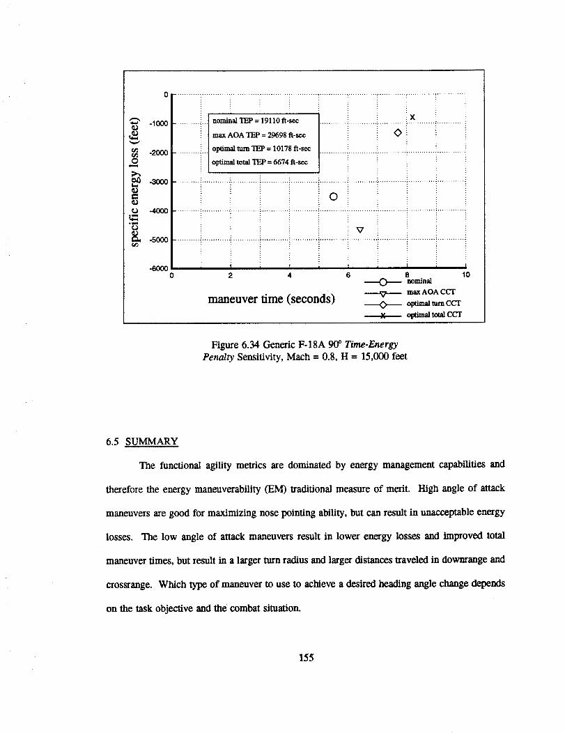
o

-1000

-2000

-3OOO

-4OOO

-5000

..........i...................................................i...................................................i...........

..........i...loo,_,,,_=,o,,o_-s_.............i.............i.............;.x.........i.............

L .......... i'" optimal mrn TEP= 10178 fl-sec ............. iI............. i............. i ............ i............. i

....................................... , ............ , ............. . ...................................... , ..........................

©

v

-6000 i I i T i t0 2 4 6

maneuver time (seconds)

i I i I8 10

0 no_a]max AOA CCT

--"0---- ovtin_ tam ccrX oFim_totalCCT

Figure 6.34 Generic F-lgA 90° Time-Energy

Penalty Sensitivity, Mach = 0.8, H = 15,000 feet

6.5 SUMMARY

The functional agility metrics are dominated by energy management capabilities and

therefore the energy maneuverability (EM) traditional measure of merit. High angle of attack

maneuvers axe good for maximizing nose pointing ability, but can result in unacceptable energy

losses. The low angle of attack maneuvers result in lower energy losses and improved total

maneuver times, but result in a larger turn radius and larger distances traveled in downrange and

crossrange. Which type of maneuver to use to achieve a desired heading angle change depends

on the task objective and the combat situation.

155

The functionalagilitymetricstestedherecannotfullyaddressthehigh angleof attack

controllabilityissueand itseffectupon maneuvering capability.This isdemonstratexlby the

inabilityof the functionalagilitymetricsto highlightthe unconventionaldesign features

incorporatedin theX-29A, e.g.good highangleof attacklateralcontrol,and reducedtrimdrag

in the transonic and supersonic flight regimes. These aspects tend to lend themselves better to

analysis using the lateral agility metrics in Chapter 4. However, the functional agility metrics did

indicate that the generic X-29A has energy bleed rates at elevated angles of attack similar to other

fighter aircraft.

None of the functional agility metrics studied take into account the turn radius of a given

maneuver, which is an important parameter. A metric that directly combines the turn radius,

maneuver time, and energy efficiency for a given maneuver into one parameter would be very

useful but is beyond the scope of the current study.

Within their limitations, the functional agility metrics are useful measures of maneuvering

capability. The strength of this class of metrics is:

.

*

o

the direct measurement of the capability to quickly transition

between two distinct maneuvering states

representation of tasks relevant to air combat maneuvering, in a

format readily accessible to pilots

measurement of the efficiency of a given maneuver, in addition

to assessing the agility of the airframe.

The results presented for each of the functional agility metrics tested in Section 6.4

demonstrate that they are highly sensitive to the particular pilot command input strategy used.

These sensitivities can cause large changes in the measured value for each metric, but also offer

156

insight into the efficiency of different air combat maneuvers for a given aircraft. The sensitivity

also makes it difficult to use these metrics for direct comparisons between aircraft without

establishing a common test strategy, not just a common test pilot command input strategy. The

example of using the 180 ° combat cycle time meu'ic to compare the generic F-16A and generic

F-18A illustrates that a standardized command input strategy can inadvertently favor a given

aircraft and bias the results. This is because the aircraft which does not have an angle of attack

limiter (e.g. the generic F-18A) might be judged inferior due to large energy losses during the 180

degree heading angle change, compared to an aircraft which has an angle of attack Umiter (e.g.

the generic F-16A). The use of an optimal angle of attach schedule resulted in marked

improvements in the measured agility of the generic F-18A, while still complying with the test

criteria.

From results obtained using the generic F-18A, the seusitivilies of the functional agility

metrics as a class can be summarized as follows:

°

°

°

.

.

the measured values of the functionai agility metrics are a strong

function of angle of attack, while bank angle errors and throttle

setting have only a small effect.

low angle of attack maneuvers provide the lowest measuredvalues of the metrics, but may not best the "best" maneuvers for

a given combat situation.

high angle of attack nose pointing maneuvers result in largemeasured values of the metrics, but maximize nose pointing

capability (small time to kill).

by following an optimal angle of attack schedule, it is possibleto reduce total energy losses and bleed rates as much as 80%,

and improve the measured value of some metrics by 60%.

the time to capture a 180 ° heading angle change (time to kill) can

be reduced 40% by using the maximum available angle of atlack.

157

7. CONCLUSIONS

Instead of supplying specific, detailed conclusions about the relevance or utility of one

candidate metric versus another one, the authors have attempted to provide sufficient data and

analyses for readers to formulate their own conclusions. Readers are ultimately responsible for

judging exactly which metrics are "best" for their particular needs. The following general

conclusions on fighter agility, based upon the experiences of all researchers who participated in

the investigation, are as follows.

1) The study of agility uses conventional airplane dynamics that are well known and

understood. It does not require a "new look" at the airplane equations of motion.

Agility is some unspecified combination of transient performance and flying

qualities. Besides the obvious impact of transient performance on agility, flyingqualities serve to identify the fastest dynamics that pilots can use effectively.

2) Agility metrics are most useful when they measure combat relevant tasks. Thetask oriented measures of agility are usually straightforward to test and measure

since they are well defined. Metrics which emphasize large instantaneous rates

and accelerations are not true reflections of the quicker time to complete a task.

Acceleration is just one aspect of transient performance. Emphasizing maximum

values ignores the associated problem of reductions in controllability. However,it has been shown that task oriented metrics can in some cases be unintentionally

aircraft specific, usually due to prescribed initial and final conditions.

3) No single candidate agility metric investigated in this report is completely

adequate, by itself, for quantifying the combat capabilities of fighter aircraft in a

modem, within visual range (WVR) air combat environment. Each candidate

metric provides a different insight into the complex issue of agility.

4) With the exception of the functional metrics and instantaneous metrics, eachcandidate agility metric is categorized according to a single aircraft axis. The axis

selected represents the axis in which the (intended) motion occurs. However, the

metrics categorized according to axis tend not to be truly uncoupled from theother axes.

158

5) The usefulness and/or relevance of any one candidate agility metric cannot be

determined by applying it to only one type of aircraft. The results in this report

clearly demonslrate that results can vary widely between aircraft types for thesame melric.

6) In addition to the sometimes obvious contributions of the airframe and powerplant

to the overall agility level of an aircraft, the details of the flight conlrol system

have a major impact on the agility (or lack of agility) that an aircraft possesses.

7) Aircraft design involves compromises between many conflicting requirements.

Once a particular class or set of candidate agility me_cs is selected, it is possible

to incorporate them as performance requirements when specifying airframe/flight

controller design specifications, even if not as a formal specification such as a

military specification. Using only minor changes (increased rudder rate, largerrudder on the same vertical tail, and modified roll command limiters), aircraft

which were designed without an specific agility requirement can in some cases

have their existing level of agility improved. An example of how the existing

agility of an aircraft can be improved is given in Reference 26.

8) The sensitivity of the candidate agility metrics to deviations in pilot command

inputs varies widely. The range is from low sensitivity (pitch metrics), to

medium sensitivity and reliance on algorithms (lateral metrics), to highly sensitive(functional metrics). Therefore agility melrics as a whole cannot reliably be

classified as having a single, common degree of sensitivity.

9) All of the candidate agility metrics investigated in this report are straightforwardto measure and test using non real-time flight simulation. Since the metrics are

well defined and existing standard flight test instrumentation is sufficient,

extension of the testing and measurement procedures in this report to piloted

simulators and actual flight testing should not impose reqmr' ements for

instrumentation or sensors currently available on high performance test aircraft.

lO) The axial agility melrics (power onset parameter and the power loss parameter)

do not quantify the acceleration capability of an aircraft. They highlight instead

the desirable qualifies of short engine spool up and down times and the

effectiveness of drag producing devices. In general, the aircraft with the faster

spooling engine and the more effective speedbrakes tends to have greater axial

agility than the aircraft which is superior in acceleration.

159

11) With the exception of the time to maximum normal load factor metric, the pitch

agility metrics as a class apply to dissimilar aircraft comparisons, and are

straightforward for pilots to flight test. Extraction of useable data from flight test

for measuring the load factor rate metric may require unique data reductionmethods. As tested on the generic F-18A, all of the pitch agility metrics

investigated are largely insensitive to deviations in pilot command inlmts.

12) Lateral agility metrics tend to be representative of the pilot tasks and

nonsymmetrical maneuvering demands of modem air combat. The time throughroll angle metrics are useful for measuring the transient performance aspect of

agility, and the roll angle capture metrics incorporate flying qualifies to a certain

extent. Although the lateral agility metrics tend to become more sensitive to

deviations in pilot command inputs with increasing angle of attack, the effects canbe largely corrected by the data reduction algorithm discussed in Chapter 4.

13) The functional agility metrics are measures of the efficiency of a given maneuver,in addition to measures of airframe agility. The use of high angle of attack

command input strategies for evaluating the functional agility metrics provides

good nose pointing ability, but tends to result in unacceptable energy losses.

Trajectory optimization routines can provide command input slrategies (optimal

angle of attack schedules) which lead to significant reductions in the functional

agility metric values for a given aircraft. Maneuvers which track an optimal angle

of attack schedule result in lower energy losses and improved total maneuver

times, but result in larger turn radius values and larger distances lraveled in

downrange and crossrange. The task objective and combat situation would dictate

which strategy is best to use for a given situation. The functional agility metrics

as a class are very sensitive to variations in pilot command input strategy.

14) The instantaneous agility metrics, curvature agility and Herbst torsional agility,

are of the open loop, maximum value, "more is better" type. Since no practical

upper limits on the measured values of these two metrics are imposed, care mustbe taken when interpreting results and drawing conclusions based upon them.

Curvature agility and Herbst torsional agility are well approximated by maximum

rate of change of normal load factor and maximum wind axis roll rate

respectively.

160

8. RECOMMENDATIONS

Based on the results of this report, several promising areas for fu_er investigation have

been identified.

I) The value that increased agility holds for air combat effectiveness should be

investigated. The differences in levels of agility must be correlated with the

experiences of the pilots who employ the aircraft in operational air-to-air and air-

to-ground missions. Further study of the promising candidate agility metrics

studied so far under this project should be conducted on a manned fight simulator.This information can then be used to help set priorities and goals for designing

more agility into fighter aircraft.

2) The ail_ame design compromises necessary to achieve various levels of agility

should be investigated, especially large control surfaces and fast actuator rates.

With regard to lateral agility, focus on ways to increase both roll and yaw control

power and how to coordinate them during a rolling maneuver. A study of the

generic F-18A showed that lateral agility on that aircraft can be improved throughbetter coordination of the ailerons and rudders (REF. 26). A similar analysis on

a different aircraft, one which already possesses good aileron-rudder coordination,

might highlight different areas for improvement.

3) Flight control system design can directly enhance the agility of fighter aircraft.

Techniques which appear promising for improving agility include:

i) striving for control harmony by trying variouscombinations of rudder and actuator rates until a

combination which enhances agility is obtained.

ii) feedbacks to the rolling surfaces to coordinate

rolls at high angles of attack.

i_) using rudder to generate proverse yawingmoments and to damp lateral and directional

oscillations at high angles of attack.

4) The benefits of increased nose down pitch agility on air combat effectiveness

should be determined. NASA Langley has also expressed renewed interest (May

1991) in the capability of pitching down to zero g from a high angle of attackattitude.

161

5) Standardized test procedures for testing different aircraft types should be

developed, especially for the functional agility metrics. In this regard, the OTIS

program can be used to study the feasibility of automatically flying agility

maneuvers. These optimal maneuvers could also be used to provide information

for designing flight control limiters and pilot displays. The OTIS program canalso be used for optimization of high angle of attack maneuvers, such as the

Herbst maneuver. By calculating the functional agility metrics for this maneuver,

it could be compared to other conventional maneuvers to study energy loss,

heading capture time, and total maneuver time.

6) Determine whether axial accelermion capabilities or axial agility capabilities is

most important in modern air combat. The less desirable characteristic can

pr_)bably be discarded all together.

7) Most of the candidate agility melrics investigated in this report exhibited

significant multi-axis effects. These multi-axis effects should be carefullyexamined and given due consideration when interpreting results and drawing

conclusions.

8) Aerodynamic data thatincludesunsteady and aero-elasticeffectsshould be

incorporatedintoflightsimulationprograms which areused forstudyingagility

metrics.This can helpdeterminewhat influencethesenonlinearaerodynamic

effects might have on the values of the metrics.

9) The functional agility metrics studied in this report do not take into account the

turn radius of a given maneuver, which can be a significant consideration. A new

metric, or a modified version of an existing one, that directly combines the turn

radius, maneuver time, and energy efficiency for a given maneuver into one

parameter might be useful.

162

9. REFERENCES

. Liefer, Randall K., Valasek, John, Eggold, David P., and Downing, David R., ',Fighter

Agility Metrics, Research and Test," Journal Of Aircraft, Vol. 29, No. 3, May-Jtm.

1992, pp. 452-457.

. Liefer, Randall IC, Valasek, John, Eggold David P., and Downing, David R.,

"Assessment of Proposed Fighter Agility Metrics," AIAA-90-2807-CP, AIAA

Atmospheric Flight Mechanics Conference, Portland, OR, Aug. 1990.

. Liefer, Randall K., "Fighter Agility Melrics," University Of Kansas Flight Research

Laboratory, KU-FRL-831-2, Lawrence, KS, Jan. 1990.

. Skow, Andrew M., and Hamilton, W. L., "Advanced Fighter Agility Metrics," Eidetics

International Technical Report TR84-05, Hawthorne, CA, Sept. 1984.

° Dorn, Matthew D., "Aircraft Agility: The Science and the Opporttmities," AIAA-89-

2015-CP, AIAA/AHS/ASEE Aircraft Design, Systems and Operations Conference,

Seattle, WA, Jul. 1989.

Valasek, John, and Eggold, David P., "Fighter Agility Metrics Research At The

University Of Kansas," AIAA Wichita Section XVI Annual Teehnologyfest, Wichita,

KS, Nov. 1989.

. Valasek, John, "A Study Of A Proposed Modified Torsional Agility Metric," AIAA-

91-2883-CP, A/AA Atmospheric Flight Mechanics Conference, New Orleans, LA,

Aug. 1991.

. Valasek, John, "SIM-II Generic F-18 Flight Simulation Program Documentation,"

University Of Kansas Flight Research Laboratory, KU-FRL-831-1, Lawrence, KS,Jun. 1990.

, Paris, S.W., Hargraves, C.R., and Martens, P.J., "Optimal Trajectories By Implicit

Simulation Version 2.0 Formulation Manual," Boeing Aerospace and Electronics,

Seattle, WA, 1990.

163

10. Vlases, W.G., "Optimal Trajectories By Implicit Simulation Version 2.0 User's

Manual," Boeing Aerospace and Elec_onics, Seattle, WA, 1990.

II. Foltyn, R.W., et. al., "Development of Innovative Air Combat Measures of Merit for

Supermaneuverable Fighters," Air Force Wright Aeronautical Laboratories, Dayton,OH, AFWAL-TR-87-3073, Oct. 1987.

12. Lynch, Urban H.D., et. al., "Tactical Evaluation of the Air-to-Air CombatEffectiveness of Supermaneuverability," WRDC-TR-90-3035, Jun. 1990.

13. Herbst, Wolfgang B., and Krogull, B., "Design For Air Combat", Journal Of Aircraft,

Vol. 10, No. 4, Apr. 1973, pp. 247-253.

14. Herbst, Wolfgang B., "Supermaneuverability," Joint Automatic Contlol Conference,

Charlottesville, VA, Jun. 1981.

15. HerbsL Wolfgang B., "Dynamics of Air Combat," Journal of Aircraft, Vol. 20, No.7, lul. 1983, pp. 594-598.

16. Herbst, Wolfgang B., "Future Fighter Maneuverability for Air Combat," AIAA

Design, Systems and Operations Meeting, Oct. 1983.

17. Hodgkinson, John, el. al., "Relationships Between Hying Qualities, Transient Agility,

and Operational Effectiveness of Fighter Aircraft," AIAA-88-4329-CP, AIAA

Atmospheric Flight Mechanics Conference, Minneapolis, MN, Aug. 1988.

18. Skow, Andrew M., el= al., "Transient Agility Enhancements for Taclical Aircraft, Vol.

III," Eidetics International Technical Report TR89-001, Hawthorne, CA., Jan. 1989.

19. Riley, David R., and Drajeske, Mark H., "An Experimental Investigation of Torsional

Agility in Air-to-Air Combat," AIAA-89-3388, AIAA Atmospheric Flight MechanicsConference, Boston, MA, Aug. 1989.

20. Small, Lester L., and Liston, Glenn W., "Impact of Pitch/Yaw Vectoring Nozzles on

Close-In Fighter Combat," Wright Research and Development Center, Oct. 1990.

164

21. Herbst, Wolfgang B., "X-31A," SAE-871346, _ National Aerospace ElectronicsConference, 1987.

22. Ray, B.S. and Cord, Thomas J. "Supermaneuverability and Hying Qualities Issues,"

National Aerospace Electronics Conference, 1986.

23. Sweetman, Bill "X-31; Through the Grape Barrier," Interavia, Oct. 1987, pp. 475-476.

24. Brown, Paul T., Hardeman, J.W., Ross, M.L., Albrecht, B.R., Fortmann, K.M., and

Zeis, J,E. Jr., "T-38A/F-16B Agility Metrics Evaluation (Agile Lightning)," USAFTest Pilot School Technical Report USAFTPS-TR-87A-SO4, Dec. 1987.

5. Butts, Smart L. and Lawless, Alan R. "Flight Testing for Aircraft Agility," AIAA-90-1308-CP, AIAA/SFTE/DGLR/SETP Fifth Biannual Flight Test Conference, May

1990.

26. Eggold, David P., Valasek, John, and Downing, David R., "Measurement and

Improvement of the Lateral Agility of the F-18," Journal of Aircraft, Vol. 30, No. 6,Nov.-Dec. 1993.

27. Eggold, David P., Valasek, John, and Downing, David R., "The Measurement and

Improvement of the Lateral Agility of the F-18," AIAA-91-2880-CP, AIAAAtmospheric Flight Mechanics Conference, New Orleans, LA, At/g. 1991.

28. Eggold, David P., "The Assessment and Quantification of Lateral Agility Metrics

Using an F-18 Simulation," University Of Kansas Flight Research Laboratory, KU-FRL-831-4, Lawrence, KS, Sept. 1990.

29. Dorn, Matthew D., "The Science of Aircraft Agility: A Framework for Classification

and Exploration," AIAA Aerospace Engineering and Conference Show, Feb. 1989.

30. Tamrat, B.F., "Fighter Agility Assessment Concepts and Their Implications on Future

Agile Fighter Design," AIAA-88-4400-CP, AIAA Aircraft Systems, Design and

Operations Meeting, Sept. 1988.

31. Spearman, M. Leroy, "Some Fighter Aircraft Trends," AIAA-g4-2503-CP, AIAA

Aircraft Design, Systems and Operations Meeting, San Diego, CA, Nov. 1984.

165

32. Bitten, Robert, "Qualitative and Quantitative Comparison of Government and Industry

Agility Metrics," AIAA-89-3389-CP, AIAA Atmospheric Flight Mechanics

Conference, Boston, MA, Aug. 1989.

33. HerbsL Wolfgang B., "Agility," Workshop On Agility Metrics, Air Force FLight TestCenter, Edwards AFB, CA, Mar. 1988.

4. Riley, David R., and Drajeske, Mark H., "Relationships Between Agility Metrics and

Flying Qualities," SAE Paper 901003, SAE Aerospace Atlantic, Dayton, OH, Apr.1990.

35. Ka]viste, JurJ, "Measures of Merit for Aircraft Dynamic Maneuvering," SAE Paper

901005, SAE Aerospace Atlantic, Dayton, OH, Apr. 1990.

36. Schweikhard, William G., Kohiman, D.L., "Flight Test Principles and Practices Short

Course Notes," University Of Kansas Division of Continuing Education, May 1990.

37. Hoffler, Keith, Ogburn, M., and Nguyen, L., "High-Alpha ControlRequirements,"

NASA High- Alpha Technology Program Workshop, Dryden Flight Research Facility,

Nov. 1989.

38. Valasek,John,"A Study Of A ModifiedTorsionalAgilityMetricUsing Simulation

Methods," UniversityOf Kansas FlightResearch Laboratory,KU-FRL-831-3,

Lawrence,KS, Oct.1990.

39. Anonymous, "F-5A/E Technical Description," Northrop Corlx_ation Aircraft Division,

Northrop Report 71-20, Hawthorne, CA, Jul. 1973.

0. Anonymous, "Military Standard - Flying Qualities of Piloted Vehicles," MIL-STD-1797-A, Mar. 1987.

41. Cannon, John D., "Predicting The Victor," AIAA-91-0418-CP, 29th AIAA Aerospace

Sciences Meeting, Reno, NV, Jan. 1991.

2o Ryan, George W. 111,and Downing, David R., "The Evaluation of Several FunctionalFighter Agility Metrics Using Optimal Trajectory Analysis Techniques," AIAA-92-

4488-CP, AIAA Atmospheric night Mechanics Conference, Hilton Head Island, SC,

Aug. 1992.

166

43. Cox, Brian W., "Evaluation of Several Functional Agility Melrics For Fighter Class

Aircraft," MS Thesis, University of Kansas Department of Aerospace Engineering,

Lawrence, KS, Aug. 1991

4. Humphreys, Robert P., Hennig, G.R., Bolding, W.A., and Helgeson, L.A., "Optimal3-Dimensional Minimum Time Turns for an Aircraft," The Journal of the

Astronautical Sciences, VoL XX, No. 2, Sept.-Oct. 1972, pp. 88-112.

5o Well, K.H., and Berger, E., "Minimum-Time 1800 Turns of Aircraft," Journal of

Optimization Theory and Applications, Vol. 38, No. 1, Sept. 1982, pp. 83-97.

46. Schneider, Garret L., and Watt, George W., "Minimum Time Turns Using Vectored

Thrust," Journal of Guidance, Control, and Dynamics, Vol. 12, No. 6,

Nov.-Dec., 1989.

7. McAtee, Thomas P., "Agility-Its Nature And Need in the 1990's," The Society of

Experimental Test Pilots Symposium, Sept. 1987.

48. Lawless, Alan R., "Aircraft Agility Measurement Research and Development,"

AFFIC-TIM-91-01, Jun. 1991.

49. Cox, Brian W., and Downing, David R., "Evaluation of Functional Agility Metrics

For Fighter Class Aircraft," AIAA-92-4487-CP, AIAA Atmospheric Flight Mechanics

Conference, Hilton Head Island, SC, Aug. 1992.

50. Skow, Andrew M., "Agility As A Contributor To Design Balance," Journal Of

Aircraft, Vol. 29, Jan.-Feb. 1992, pp. 34-46.

51. PersonalConversationwithMajor Bob Vosburgh,USAF, Iowa StateUniversityAir

Force ROTC, Oct.1990.

52. Personal Conversation with Major Dale A. Nag),, USAF, United States Air Force

Academy, Nov. 1990.

53. Ryan, George Wesley HI, "The Evaluation of Several Functional Agility Metrics

Using Optimal TrajectoryAnalysisTechniques,"MS Thesis,Universityof Kansas

Departmentof AerospaceEngineering,Lawrence,KS, Apr. 1992

167

54. McAtee, Thomas P., "Agility in Demand," Aerospace America, May 1988, pp. 36-38.

55. Shaw, Robert L., FIGHTER COMBAT Tactics and Maneuvering, Naval Institute

Press, Annapolis, MD, 1985.

56. Personal Conversation with Joe Wilson, NASA-Ames Dryden Flight Research Facility

(XRDD), May 1991.

57. Dorn, Matthew D., "EIGHT IDEAS Toward an Aircraft Agility Theory," a USAF

Flight.Dynamics Laboratory White Paper, 1989.

58. Anonymous, "Military Specification, Flying Qualities of Piloted Airplanes," MIL-F-

8785C, Nov. 1980.

59. Anonymous, "Military Specification, Flying Qualities of Piloted Airplanes," MIL-F-

8785, Sept. 1954.

60. Anonymous, "Military Specification,FlyingQualitiesofPiloted Airplanes," MIL-F-

8785B, Aug. 1969.

61. Lockenour, Jerry L., "Northrop Review of MIL-F-8785B Proposed Revisions,"

Proceedings of AFFDL Flying Qualities Symposium Held at Wright State University

12-15 Sep. 1978, AFFDL-TR-78-171, Dec. 1978, pp. 260-282.

62. Moorehouse, David J., Woodcock, R.J., and Sweeney, T.P., "Discussion and Status

of the Proposed Revision (1978) to MIL-F-8785B," Proceedings of AFFDL Flying

Qualities Symposium Held at Wright State University, 12-15 Sept. 1978, AFFDL-TR-

78-171, Dec. 1978, pp. 236-250.

63. Chalk, Charles R., Neal, T.P., Harris, T.M., Pritchard, F.E., and Woodcock, R.J.,

"Background Information and User Guide For MIL-F-g795B(ASG)," Air Force Flight

Dynamics Laboratories, Dayton, OH, AFFDL-TR-69-72, Aug. 1969.

4°

65.

Lipschutz, NL M., Differential Geometry, Mc-Graw Hill, New York, NY 1969.

Stoker, J. J., Differential Geometry, Wiley Interscience, New York, NY, 1969.

168

66. Baker, Dick, "Aircraft Time History Program," Sperry Support Services, Langley

Operations, Report Number SP-205-, Hampton, VA, Jan. 1979.

67. Angelucci, Enzo, and Bowers, P., The American Fighter, Orion Books, New York,

NY, 1985.

68. Linn, Don, The F-18 Hornet In Detail & Scale, Tab Books Inc., Blue Ridge

Summit, PA, 1982.

69. Reports and Presentations Branch, NASA-Ames Dryden Flight Research Facility,Edwards, CA.

70. Etkin, Bernard, Dynamics of Atmospheric Flight, John Wiley & Sons, New York,1972.

71. Anonymous, "USAF Test Pilot School FLYING QUALITIES TEXTBOOK VOLUME

II Pan 2," USAF-TPS-CUR-86-03, Apr. 1986.

72. Blakelock, John, Automatic Control of Aircraft and Missiles, John Wiley & Sons,

New York, 1965.

73. Nguyen, Lnat T., Gilbert, William P., and Ogburn, Marilyn E., "Control-System

Techniques For Improved Departure/Spin Resistance For Fighter Aircraft," NASA TP-

1689, Aug. 1980.

74. Chalk, Charles R., "The Ideal Controlled Element for Real Airplanes is Not K/s,"

Calspan FRM No. 554, Aug. 1981.

75. Monagan, Stephen J., Smith, R.E., and Bailey, R.E., '1.,ateral Hying Qualities of

Highly Augmented Fighter Aircraft," Air Force Wright Aeronautical Laboratories,

Dayton, OH, AFWAL-TR-81-3171, Vol. I, Jtm. 1982.

76. Hoh, Roger H., Mitchell, D.G., Aslakenas, I.L., Klein, R.H., Heffley, R.K., and

Hodgkinson, J., "Proposed MIL Standard and Handbook -Flying Qualities of AirVehicles, Volume H: Proposed MIL Handbook," Air Force Wright Aeronautieai

Laboratories, Dayton, OH, AF'_AL-TR-82-3081 VOLUME II, Nov. 1982.

169

77. Whitley,PhillipB., "Human Capabilities in Highly Agile Aircraft," SAE Aerospace

Atlantic Conference, Dayton, OH, Apr. 1990.

78. Lan, Chuan-Tau, and Roskam, J., Airplane Aerodynamics and Performance,

Roskam Aviation and Engineering Corporation, Ottawa, Kansas, 1980.

In addition to the numbered references, the researchers and contributors to this report have

found the following reports and documents useful in the study of agility, and recommend them to the

interested reader:

Aircraft Agility WORKshop," Air Force Wright Research and Development Center, Aug. 1989.

Anderson, John, "Agile Fighter Aircraft Simulation," AIAA-89-0015-CP.

Barnes, A.G., "The Study of Combat Aircraft Manoeuvrability by Air To Air Combat Simulation,"

British Aerospace Public Limited Company, Warton Division, Preston, Lancashire, England.

Beaufrere, Henry, "Integrated Flight Control System Design for Fighter Aircraft Agility," AIAA-88-

4503-CP, Aircraft Design, Systems and Operations Meeting, Sep. 1988.

Bihrle, William Jr., and Barnhart, B., "Departure Susceptibility and Uncoordinated Roll-Reversal

Boundaries for Fighter Configurations," Journal of Aircraft, Vol. 19, No. 11, Nov. 1982.

Bise, Michael E., Black, Thomas G., "Is Agility Implicit in Flying Qualities?," Proceedings of the

1990 IEEE National Aerospace and Electronics Conference, Dayton, OH, May 1990.

170

Bran, R.W. and Johnston, E.W., "Technology Analysis - Candidate Advanced Tactical Fighters,"

AIAA-78-1451-CP, AIAA Systems and Technology Meeting, Aug. 1978.

Chin, J., "X-29A Flight Control System Performance During Flight Test," AIAA-87-2878-CP, AIAA

Aircraft Design, Systems and Operations Meeting, Sep. 1987.

Chin, Hubert H, "A Knowledge Based System for Supermaneuver Selection for Pilot Aiding," AIAA-

88-4442-CP, AIAA Aircraft Design, Systems and Operations Meeting, Sep. 1988.

Chody, Joseph R., Hodgkinson, John, and Skow, Andrew M., "Combat Aircraft Control Requirements

for Agility," Aerodynamics of Combat Aircraft Controls and of Ground Effects, AGARD-CP-465, Apr.1990.

Conrady, Neal, Baron, Timothy, and Fu, Johnny S., "Local Adaptive Maneuvering Optimization for

Fighter Aircraft," AIAA-90-3453-CP, AIAA Atmospheric Flight Mechanics Conference, Portland, OR,

Aug. 1990.

Cord, Thomas J., Detroit, Mark J. and Muithopp, Dieter, "Is An Agility Requirement Needed for

Fighter Agility," SAE Aerospace Atlantic Conference, Dayton, OH, Apr. 1990.

Cord, Tom J., "A Standard Evaluation Maneuver Set for Agility and the Extended Flight Envelope -

An Extension to HQDT," AIAA-89-3357-CP, AIAA Atmospheric Flight Mechanics Conference,

Boston, MA, Aug. 1989.

EtheU, Jeffrey L., "Radar Combat and the Illusion of Invincibility," Aerospace America, Jan. 1990,pp. 14-18.

Foltyn, R.W., et al., "Innovative Cockpit Display and Cuing Systems for Operation in an Extended

Flight Envelope." NASA-TR-87-215.

Gilbert, W.P., "Overview of NASA High-Alpha Technology Program (HAFt)," High AlphaTechnology Program Workshop, Nov. 1989.

Henri, A.W., "Review of Practical Experience on Combat Aircraft Maneuverability," RoyalNetherlands Air Force.

Herbst, Wolfgang B., "Future Fighter Technologies," Journal of Aircraft, Vol. 17, No. 8, Aug. 1980.

171

Herrick, Paul W., "Propulsion Influences on Air Combat," AIAA-85-1457-CP, AIAA Joint PropulsionConference, Jul. 1985.

lnnocenti, Mario, "Metrics for Roll Response Hying Qualifies," Flying Qualities, AGARD-CP-508,

Feb. 1991, pp. 14-1 to 14-11.

Juang, Jyh-Ching and YusseL Hussein M., "Aircraft Agility," Lockheed Aeronautical Systems

Company, Burbank, CA, 1990.

Johnston, Donald E., "High AOA Lateral-Directional Design Guides and Criteria - A Piloted

Simulation Assessment," Proceedings of AFFDL Flying Qualities Symposium Held at Wright-Patterson Air Force Base in October 1979, AFWAL-TR-80-3067, May 1980, pp. 9-28.

Kalviste, Juri, "Spherical Mapping and Analysis of Aircraft Angles for Maneuvering Flight," Journal

of Aircraft, Vol. 24, No. 8, Aug. 1987.

Kalviste, Juri, "Roll Reversal Agility Parameter," Air Force Flight Dynamics Laboratories, Dayton,

OH, AFFDL Aircraft Agility Workshop Summary Booklet, Aug. 1989.

Kato, Osamu, "Attitude Projection Method for Analyzing Large-Amplitude Airplane Maneuvers,"

Journal of Guidance, Control, and Dynamics, Vol. 13, No. 1, Jan.-Feb. 1990, pp. 22-29.

Kocher, James A., "Integrated Conlrol and Avionics for Air Superiority: A Program Overview," SAE

Paper 901049, SAE Aerospace Atlantic Conference, Dayton, OH, Apr. 1990.

Liu, Hung-Chi, "Development of Trim States and Linear Models From Nonlinear Simulations," MS

Thesis, University of Kansas Department of Aerospace Engineering, Lawrence, KS, Dec. 1991

Madelung, Gero, "Characteristics of Fighter Aircraft," AIAA-77-1219-CP, AIAA Aircraft Systems and

Technology Meeting, Seattle, WA, Aug. 1977.

Mayer, John P., and Hamer, H.A., "A Study of Service-Imposed Maneuvers of Four Jet Fighter

Airplanes in Relation to Their Handling Qualities and Calculated Dynamic Characteristics," NACA

RM L55E19, Aug. 1955.

Mazza, C.J., "Agility: A Rational Development of Fundamental Metrics and their Relationship to

Hying Qualities," Flying Qualities, AGARD-CP-508, Feb. 1991, pp. 27-1 to 27-7.

172

McKay,IC, andWalker,M.J., "A Review of High Angle of Attack Requirements for Combat

Aircraft," Flying Qualities, AGARD-CP-508, Feb. 1991, pp. 28-1 to 28-12.

Myers, T.T., McRuer, D.T., and Johnston, D.E., "Flying Qualities Analysis for Nonlinear Large-

Amplitude Maneuvers," AIAA-87-2904-CP, AIAA/AHS/ASEE Aircraft Design, Systems and

Operations Meeting, St- Louis, MO, Sept. 1987.

Neal, T.P. and Smith, R.E., "An In-flight Investigation to Develop Control System Design Criteria for

Fighter Airplanes," Air Force Flight Dynamics Laboratories, Dayton, OH, AFFDL-TR-70-74, Dec.

1970.

Polumbo, Joke, "Lethal at the Merge...Kill and Survive," USAF Fighter Weapons Review, Summer

1992, pp. 23-25.

Raymer, Daniel P., "Post-Stall Maneuver and the Classic Turn Rate PloL" AIAA-91-3170-CP,AIAA/AHS/ASEE Aircraft Design, Systems and Operations Meeting, Baltimore, MD, Sept. 1991.

Roskam, Jan, "A Simplified Method to Identify and Cure Roll Coupling," Journal of the Aerospace

Sciences, Vol. 29, No. 5, May 1962.

Rutowski, Edward, "Energy Approach to the General Aircraft Performance Problem," Journal of the

Aeronautical Sciences, Vol. 21, No. 3, Mar. 1954, pp. 187-195.

Skow, Andrew M., "An Analysis of the Su-27 Flight Demonstration at the 1989 Paris Air Show," SAE

Paper 901001, SAE Aerospace Atlantic Conference, Dayton, OH, Apr. 1990.

Talty, P.IC and Caughling, D.J., "F-16XL Demonstrates New Capabilities in Flight Test at EdwardsAFB," Journal of Aircraft, Vol. 25, No. 3., May-Jun. 1988.

Twisdale, T. and Franklin, D., "Tracking Task Techniques for Handling Qualities Evaluations,"

AFFFC-TD-75-1, May 1975.

Walker, H.C., AFFFC Agility Flight Test Committee Meeting Minutes, Jun. 1987.

Woodcock, Robert J., "Estimation of Flying Qualities of Piloted Airplanes," Air Force Flight

Dynamics Laboratories, Dayton, OH, AFFDL-TR-65-218, Apr. 1966.

173

A. CANDIDATE AGILITY METRICS

A.1 BACKGROUND

This appendix contains a list of most of the published agility metrics and the references in

which they may be found. Each metric in this section is classified according to type, defined, and in

most cases discussed briefly. The definition used for each metric is the definition according to the

author(s) of each metric.

A.2 CANDIDATE PITCH AGILITY METRICS

Pitch agility metrics involve only pitching motion and normal acceleration.

A.2.1 Time Derivative of Load Factor (REF. 32)

Definition:

The time rate of change of normal load factor for a given maneu_,er.

Discussion:

The time derivative of load factor, though difficult to measure directly, can, in theory, be

exlracted from flight test or simulation time histories. Since both pitch up and pitch down

capability are tactically important, the rate of change of normal load factor during both types

of maneuvers should be investigated. It has been shown in Reference 32 that time histories

of normal load factor derivative and the curvature agility metric of Reference 33 are virtually

identical when scaled to account for different units.

A1

A.2.2 Time to Capture a Specified Angle of Attack (REF. 18)

Definition:

The time required to attain (pitch up and stop) maximum lift angle of attack from various

initial angles of attack.

Discussion:

During subsequent discussion of pitch agility (at the AFFDL Agility Workshop, Aug 89, for

example), t/me to capture a specified angle of attack was generally rejected as a useful metric.

Its primary disadvantage is the difficulty in accurately capturing a specified angle of attack

during flight test. A secondary disadvantage is that the time to capture angle of attack is not

an appropriate quantity for comparison among dissimilar aircraft. Also, aircraft normal

acceleration is generated by lift, which is a function angle of attack and lift curve slope. This

metric neglects the lift curve (lift versus angle of attack) characteristics of the aircraft. For

these reasons, the time to capture a specified angle of attack is not studied in this report.

A.2.3 Time to Change Pitch Attitude (REF. 24)

Definition:

The ability of an aircraft to change it's pitch angle as rapidly and precisely as possible.

Discussion:

Time to change pitch attitude has been flight tested by students at the USAF Test Pilots

School (REF. 24). During that study, pitch angle changes of -45 ° to 45 ° and -30 ° to 30° were

flown. Pilots and flight test engineers involved in that evaluation concluded that time to

change pitch attitude was unsuitable due to the large changes in airspeed and altitude that

occurred during the maneuver.

A2

A.2.4 Maximum Nose-Up and Nose-Down Pitch Rate (REF. 18)

Definition:

The maximum value of positive pitch rate attainable in transitioning from a lg flight condition

to maximum lift angle of attack; the maximum value of negative pitch rate attainable in

transitioning from maximum lift angle of attack to a Og flight conditio_

A.2.5 Pitch Agility (REF. 18)

Definition:

The sum of:

(time to pitch from a lg flight condition to maximum lift coefficient or normal load factor)

and

(Time to pitch down from maximum lift coefficient or normal load factor to 0g)

Discussion:

The authors of this metric observed that both nose up and nose down pitch agility are

important. However, a number of questions about pitch agility remain are not addressed in

Reference 18.

o

.

.

If the times associated with nose up and nose down pitch maneuvers

are to be summed, should the two be equally weighted?

Is the time to pitch up significantly different than the time to pitchdown?

Does an aircraft with better positive pitch agility necessarily have

better negative pitch agility?

Since these questions remain to be resolved by flight testers, engineers and fighter pilots,

values associated with positive pitch maneuvers and those associated with nose down pitching

are treated as separate metrics through out this report rather than summed into a single figure

A3

of merit. Though the time to achieve maximum normal load factor and the time to unload

to zero normal load factor are conceptually simple, several difficulties arise when these

metrics are evaluated with realistic aircraft models. While it is easy to initiate the pitch up

from steady level flight conditions, the pitch down from positive normal load factor may start

from a condition where airspeed and altitude are rapidly changing. If pitch agility is to be

plotted against flight condition, the choice of flight condition may often be somewhat

arbitr .a.ry.

A.2.6 Average Pitch Rate

Definition:

This metric is defined as

Average Pitch Rate

_t t2, qdt

t 2 - t I

where q is pitch rate, tl is the time at which the pitch-up is executed, and t: is the time at

which the pitch-up maneuver is completed. The completion time h is selected at the

discretion of the tester. Usually, h is selected from a common sense point of view for the

particular task which is being performed.

Discussion:

A pilot usually commands pitch rate to point the nose of the aircraft or to achieve a desired

load factor/turn rate. Ideally, pitch agility metrics should be task oriented. Measuring

maximum pitch rate capability does not relate directly to either of these tasks. Most pitch

agility metrics measure only the peak value of pitch rate that an aircraft can generate. This

is often misleading for the purpose of comparing aircraft since aircraft can only momentarily

generate very large values of pitch rate. From a task oriented point of view, it is the average

pitch rate which is desirable to measure. This metric gives some indication of how quickly

A4

a change in pitch angle can be acheived. It penalizes an aircraft which can briefly generate

a large pitch rate, and rewards the aircraft which can sustain maintain the largest values of

pitch rate over a period of time. Presentation of the average pitch rate metric are plots of

average pitch rate versus Mach number, for a specified altitude.

A.2.7 Pitch Agility Criteria or Maximum Initial Pitch Acceleration Parameter (REF. 18)

Definition:

This metric is defined as

Pitch Agility CriteriaS_Cm.

Iyy

where Cm is the nondimensional pitching moment produced by maximum deflection theaircraft's l_itch control surfaces. Here, S,'f and Iyy are standard notation for reference wing

area, mean aerodynamic chord and pitch axis moment of inertia.

Discussion:

This parameter is extracted from the expression for the dimensional pitching moment

derivative

q S_Cm.M b --

Iyy

and is a measure of the airframe's potential to generate pitch acceleration. It can be calculated

directly from aerodynamic coefficients and configuration data but does not reflect any flight

control system limits.

A5

A.3 CANDIDATE LATERAL AGILITY METRICS

Lateral agility metrics deal primarily with rolling motion, especially rolling at high angles of

attack and/or elevated normal load factors.

A.3.1 Lateral Agifity, Ttcge (REF. 18)

Definition:

The time required to roll 90 ° and stop while maintaining an angle of attack.

Discussion:

This metric is a closed loop maneuver which is a function of Mach number, altitude, and

normal load factor or angle of attack. No criteria is supplied as to what constitutes the "stop"

which terminates the maneuver. How (or should) this maneuver be compared to the more

common technique of unloading first, then rolling at one or zero g and then pitching to re-

establish the initial angle of attack is not specified. The unload-roll-load method is probably

faster especially for high angle of attack conditions. Using the loaded roll method, i.e.

holding angle of attack as constant as possible during the roll, the aircraft heading angle is

changed during the rolling maneuver. However, with the unloaded roll method the aircraft

orientation is changed but the heading angle is not rotated since the roll is accomplished while

unloaded. Manned simulation or flight test may be required to determine which pilot

technique is both easiest to test and most meaningful to the tactical (as opposed to the test)

pilot. It is the opinion of Reference 55 and others that the loaded roll is important in the

study of fighter agility since it measures the ability of the aircraft to maneuver at high angles

of attack even though it is not as commonly used by current fighters engaged in air combat

maneuvering.

A6

A.3.2 Lateral Agility, TRc_so (REF. 18)

Definition:

The time required to roll 180 ° and stop while maintaining an angle of attack.

Discussion:

This metric may be more representative of actual tactics than TRcg0. TRc_s0 is alSO a more

demanding test of the flight control system since the build up of adverse yaw will be more

pronounced over the longer maneuver.

A.3.3 Roll Angle Capture (REF. 25)

Definition:

The time required to roll and capture delta phi = 90 °, 180 °, and 360 °.

Discussion:

The TRcg0 and TRC_S0metrics introduced above are subsets of the roll angle capture metric.

The discussion involving the TRcgoand TRclso metrics can generally be applied to the roll angle

capture metric.

A.3.4 Time Through Roll Angle (REF. 58)

Definition:

The time required to roll through a target bank angle at elevated normal load factor levels.

Discussion:

Unlike the lateral agility metrics described above, the t/me through roll angle metric is

measured using open loop pilot command inputs. This metric specifies the time to achieve

A7

a specific bank angle change, initiated from a load factor of lg with wings level. The specification

states that the inputs shall be abrupt, and the pitch control input shall be fixed throughout the

maneuver. This metric has evolved into its present form from several metrics which had appeared in

earlier versions of the military specification for flying qualities of piloted airplanes (REF. 59, 60).

It is a well defined metric which specifies the class of aircraft, the flight phase, and the speed range.

These conditions were imposed on the metric to i) account for the reduction in roll response at low

and high airspeeds, ii) account for the reduction in roll response at elevated load factors, iii) require

higher response rates in the middle of the envelope for lg flight (REF. 61). Thus the bank angle

requirements were adjusted such that the bank angle change was modified to be compatible with the

speed at which the roll performance was to be demonstrated (REF. 62). The roll performance for 360 °

rolls were proposed to apply only at lg. This was done because it agreed with the current requirement

in the loads specification, and could be tested without special planning in a typical test program.

Unlike the roll angle capture metrics, the time through roll angle metric does not address the

controllability aspect of arresting the roll after the specified bank angle change has been achieved.

In spite of this, the metric is testable, repeatable, and is useful in the study of agility. Results using

this metric are presented in Chapter 4.

A.3.5 Roll Reversal Capture (REF. 25)

Definition:

The time required to roll from a 90 ° bank angle to the opposite 900 bank angle and then back

to capture the original bank angle.

Discussion:

The roll reversal capture metric is a variation of the roll angle capture metric and most likely

highlights slightly different qualities of an aircraft's transient performance. It is assumed that

A8

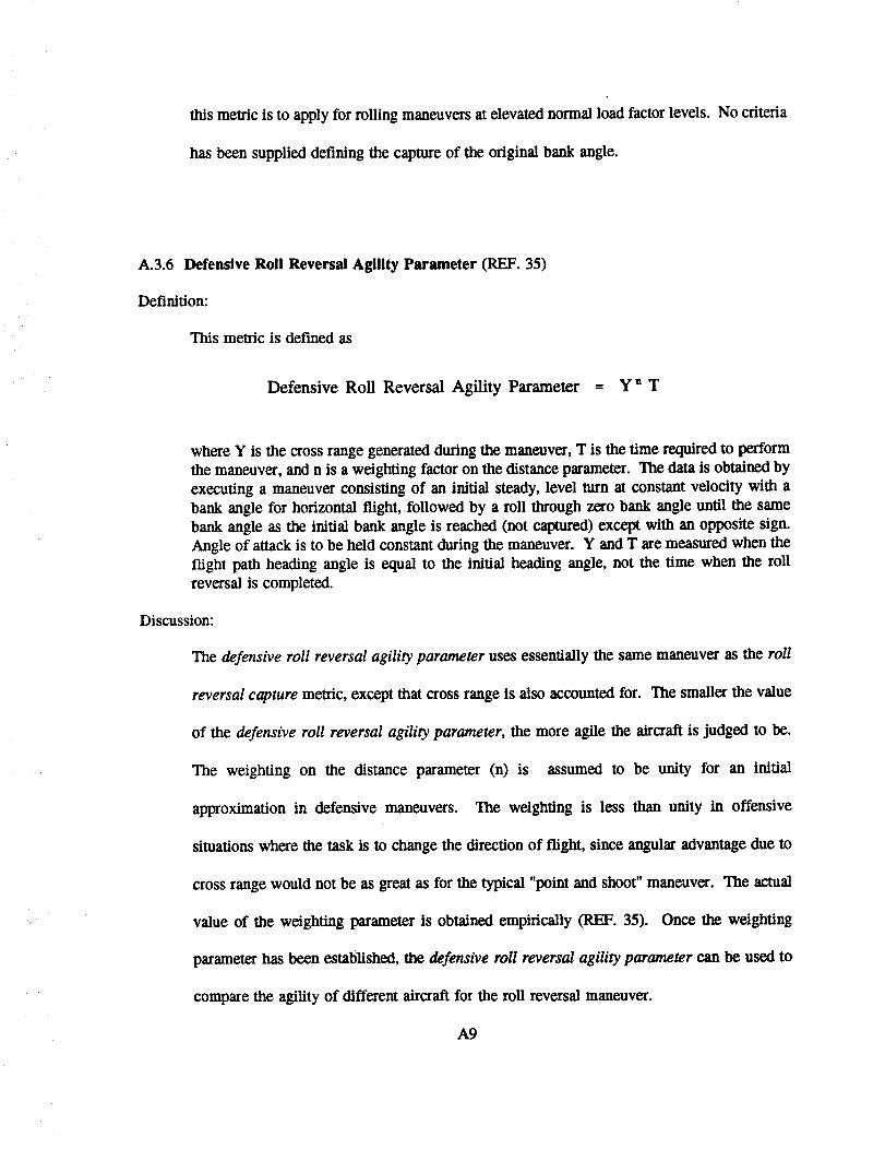
this metric is to apply for rolling maneuvers at elevated normal load factor levels.

has been supplied defining the capture of the original bank angle.

No criteria

A.3.6 Defensive Roll Reversal Agility Parameter (REF. 35)

Definition:

This metric is defined as

Defensive Roll Reversal Agility Parameter = Y*T

where Y is the cross range generated during the maneuver, T is the time required to perform

the maneuver, and n is a weighting factor on the distance parameter. The data is obtained by

executing a maneuver consisting of an initial steady, level turn at constant velocity with a

bank angle for horizontal flight, followed by a roll through zero bank angle until the same

bank angle as the initial bank angle is reached (not captured) except with an opposite sign.

Angle of attack is to be held constant during the maneuver. Y and T are measured when the

flight path heading angle is equal to the initial heading angle, not the time when the roll

reversal is completed.

Discussion:

The defensive roll reversal agility parameter uses essentially the same maneuver as the roll

reversal capture metric, except that cross range is also accounted for. The smaller the value

of the defensive roll reversal agility parameter, the more agile the aircraft is judged to be.

The weighting on the distance parameter (n) is assumed to be unity for an initial

approximation in defensive maneuvers. The weighting is less than unity in offensive

situations where the task is to change the direction of flight, since angular advantage due to

cross range would not be as great as for the typical "point and shoot" maneuver. The actual

value of the weighting parameter is obtained empirically (REF. 35). Once the weighting

parameter has been estatilished, the defensive roll reversal agility parameter can be used to

compare the agility of different aircraft for the roll reversal maneuver.

A9

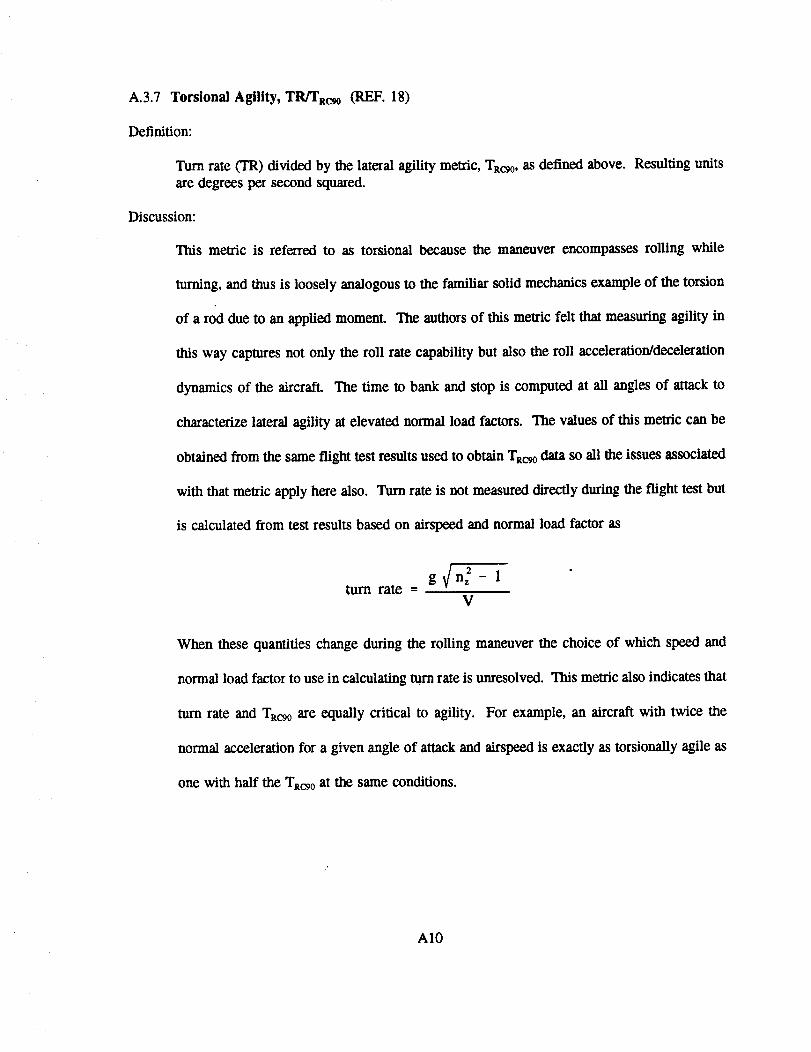
A.3.7 Torsional Agility, TR/TRcge (REF. 18)

Definition:

Turn rate OR) divided by the lateral agility metric, TRcg0, as defined above. Resulting units

are degrees per second squared.

Discussion:

This metric is referred to as torsional because the maneuver encompasses rolling while

turning, and thus is loosely analogous to the familiar solid mechanics example of the torsion

of a rod due to an applied moment. The authors of this metric felt that measuring agility in

this way captures not only the roll rate capability but also the roll acceleration/deceleration

dynamics of the aircraft. The time to bank and stop is computed at all angles of attack to

characterize lateral agility at elevated normal load factors. The values of this metric can be

obtained from the same flight test results used to obtain TRcg0data so all the issues associated

with that metric apply here also. Turn rate is not measured directly during the flight test but

is calculated from test results based on airspeed and normal load factor as

g 1turn rate =

V

When these quantifies change during the rolling maneuver the choice of which speed and

normal load factor to use in calculating turn rate is unresolved. This metric also indicates that

turn rate and TRcg0 are equally critical to agility. For example, an aircraft with twice the

normal acceleration for a given angle of attack and airspeed is exactly as torsionally agile as

one with half the TRCg0 at the same conditions.

AIO

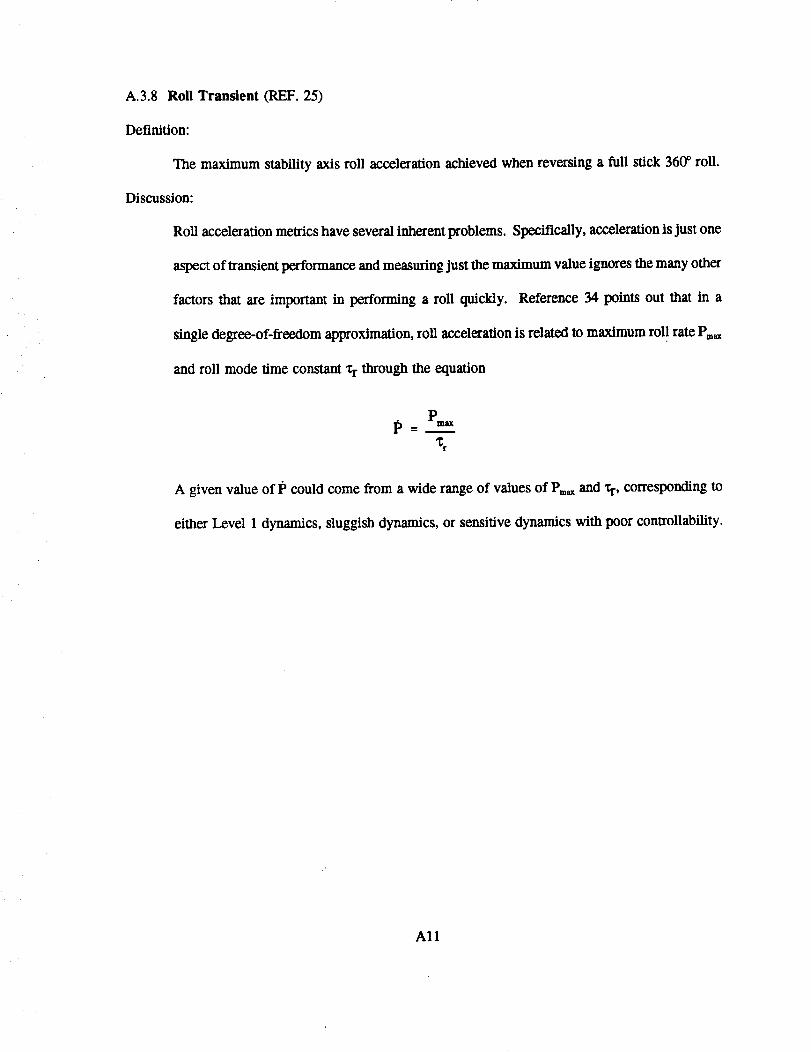
A.3.8 Roll Transient (REF. 25)

Definition:

The maximum stability axis roll acceleration achieved when reversing a full stick 360 ° roll.

Discussion:

Roll acceleration metrics have several inherent problems. Specifically, acceleration is just one

aspect of transient performance and measuring just the maximum value ignores the many other

factors that are important in performing a roll quickly. Reference 34 points out that in a

single degree-of-freedom approximation, roll acceleration is related to maximum rol! rate Pm_

and roll mode time constant x r through the equation

x,

A given value of 1_ could come from a wide range of values of P_,_ and _r, corresponding to

either Level 1 dynamics, sluggish dynamics, or sensitive dyna_cs with poor controllability.

All

A.4 CANDIDATE AXIAL AGILITY METRICS

Axial agility metrics are intended to quantify the ability of an aircraft to transition between

energy states or specific excess power (P_) levels. They involve only translational motion.

A.4.1 AxialAgility (REF. 18)

Definition:

The incremem of specific excess power (AP,) resulting in going from a minimum

power/maximum drag condition, to a maximum power/minimum drag condition, divided byAt, the time in seconds required to complete the transition (REF. 18).

A P. = P,f_ - P' _'_ (1)

At if,.m - tt,in._

Transition from minimum to maximum power is called the power onset parameter and

transition from maximum to minimum power is termed the power loss parameter.

Discussion:

Traditional methods of quantifying the axial capability (i.e. longitudinal translation capability)

of fighter aircraft have generally consisted of thrust-to-weight ratio, maximum level Mach

number, maximum rate of climb and specific excess power (P_). These point performance

measures of merit only quantify performance at discrete aircraft states and are not indicative

of the capability of an aircraft to change its energy state rapidly. Axial agility metrics are

intended to provide a measure of this capability. The axial agility metrics measure the rate

of change of P, and conform well to the idea of agility being the rate of change of

maneuverability (REF. 4). Instead of knowing only what level of P, an aircraft possesses at

a particular point, axial agility reflects how effectively the aircraft can transition to another

P, level. The power onset and power loss parameters measure the combined effects of engine

spool time, maximum thrust and drag due to speed brakes. An aircraft with good axial agility

is characterized by superior velocity control (both acceleration and deceleration).

A12

A.5 CANDIDATE FUNCTIONAL AGILITY METRICS

Functional agility metrics deal with time scales of ten to twenty seconds. This class of metrics

seeks to quantify how well the fighter executes rapid changes in heading or rotations of the velocity

vector. The emphasis is on energy lost during turns through large heading angles and the time

required to recover kinetic energy after unloading to normal load factor of zero. Many of these

• " functional agility metrics involve maneuvers made up of a sequence of brief segments of the transient

agility metrics_

A.5.1

Definition:

t_ + h_ + h2 + h + t,

t1 =

hi + h2 =

h =

h =

Combat Cycle Time (REF. 30)

where:

time to pitch from one g to the limit normal load factortime to turn to a specified new heading angle at maximum normal

load factortime to unload the aircraft to a normal load factor of one (or zero)

time to accelerate to the original energy level

Discussion:

The combat cycle time metric is characterized by a continually changing flight condition

constrained within structural, lift, and power limits. It is calculated for a given set of starting

conditions and some specified heading angle change, usually either 90 or 180 degrees. The

plot of this metric conveniently shows the relationships of normal load factor, velocity, turn

rate, and turn radius for a level turn. It is not clear whether the author of the metric intends

for the aircraft to be at the same Mach number and altitude at the end of the combat cycle or

only to have the same total energy. Times tl and h might be negligible relative to the others

A13

so this parameter is probably dominated by turn rate and Ps. Another useful feature of the

combat cycle time metric is that its maneuver cycle allows for measuring the dynamic speed

turn, relative energy state, energy-agility, and time-energy penalty metrics.

A.5.2 Dynamic Speed Turns (REF. 47, 54)

Definition:

plot of specific excess power (P_) versus maximum turn rate at a given starting airspeed.

Discussion:

This intent of this metric is to capture the dynamic maneuvering capability of fighter aircraft

(agility) as viewed from a pilots perspective, and to present that capability in a form which

can be readily used by pilots and engineers. This is accomplished by clearly showing the

bleed rate for maximum acceleration turns and the slralght and level acceleration capability

at various airspeeds. Dynamic speed turn plots show the dynamics of turning and acceleration

over a wide range of speeds, combine the ability of the aircraft to point its nose, continue

pointing its nose, and accelerate.

A.5.3 Relative Energy State, (V/V,) (REF. 30)

Definition:

The ratio of the aircraft's speed to its comer speed at completion of a 180 degree turn at

maximum g from a given starting position (altitude and airspeed). Tiffs ratio, V/Vc, should

be as close to 1.0 as possible.

Discussion:

Relative energy state is classified as a functional agility metric because it is dominated by

A14

thrust and drag characteristics. The author of this metric suggests that at least two 90 degree

turns must be made before falling below comer speed. Any speed below corner indicates that

the fighter has maximized pointing capability while exhausting maneuvering potential and

conversely, any speed above comer indicates that a fighter has not yet achieved its maximum

pointing ability in favor of retaining energy for future maneuvering. Turn rate and thus the

time required to complete the 180 degree turn are not addressed by this metric.

A.5.4 Energy-Agility (REF. 5)

Definition:

The specific energy of an aircraft during the time required to complete a maneuver, plottedas a function time.

Discussion:

This metric was developed as an attempt to model the time to kill, the time to recover, and

the energy compromised as an engineering tool. The concept for this metric was inspired by

the description of an angles fight and an energy fight (REF. 55). An angles fight is one in

which a positional advantage is sought first at the expense of energy. The purpose of the

energy fight is to garner an energy advantage over the adversary and then convert this energy

into a lethal positional advantage. The author of this metric coined the terms angles-agility

(the ability to rapidly and efficiently convert a given energy advantage into a useful positional

advantage) and energy-agility (the ability to minimize the time-energy penalty while directly

seeking a useful positional advantage) from which this metric derives its name.

A15

A.5.5 Time-Energy Penalty (REF. 43)

Definition:

This metric is def'med as

Time Energy Penalty tar * Ah,

where tA_ is the time to complete a specified heading angle change and (if required) the timeto pitch down to achieve missile envelope firing parameters, and AIM is the change in specific

energy height during the maneuver.

Discussion:

The time-energy penalty melric examines the tactically significant maneuver of heading angle

changes. This metric is essentially an extension of the combat cycle time and energy-agility

metrics with its name taken from Reference 57. The result of a direct multiplication between

tA_F and AtM is a single parameter which equally weighs the importance of minimizing time

and preserving energy during a heading change maneuver. The ideal situation is a

maneuvering aircraft which completes a short duration turn with minimal energy loss.

Conversely, an aircraft which turns slowly and depletes a large amount of energy is

undesirable. The time tAV consists of the sum of the lime to roll 90 degrees and pitch to

maximum normal load factor (tl of combat cycle time), plus the time to obtain a specified

heading angle (h of combat cycle time), plus the time to pitch down and reduce angle of

attack or normal load factor so that the missile can be fired within its envelope. The change

in specific energy height, AIM, is measured from the start of the maneuver until the time at

which the heading angle is reached and the missile envelope parameters are attained.

A16

A.5.6 DT Parameter (REF. 35)

Definition:

This metric is defined as

DTParameter -- DnT

where D is the cross range distance of the maneuver, T is the time required to perform themaneuver, and n is a weighting factor on the distance parameter. The maneuver is initiated

from straight and level flight at constant velocity. The aircraft then pitches, rolls into a limitnormal load factor level turn, and then decelerates to corner speed to achieve maximum

instantaneous turn rate. The turn is continued at constant angle of attack until the body X-axis

of the aircraft has been turned through 180 °.

Discussion:

The DT parameter is analogous to the defensive roll reversal agility parameter defined in

Section A.3.6, except that the maneuver for the DT parameter is a level 180 degree turn. This

metric is a function of Mach number, altitude, and the heading angle change of the maneuver.

It is intended to predict the "point and shoot" firing solution in engagements consisting of

aircraft which have different initial velocities and relative heading angles. Also, the difference

in DTparameters for two aircraft performing the same maneuver (ADT) predicts an advantage

for one of the aircraft, but does not relate directly to a time advantage, which is the most

important parameter. The time advantage can be computed from

AT --(DT)._r_B - (DT)tirmBA ADT

Du_t A D_t A

The AT is an approximation of the time advantage that aircraft A has over aircraft B based

on the difference in the DTparameters for the two aircraft. An important assumption which

has been made in defining a "point and shoot" maneuver such as the DT parameter is that

both aircraft have similar weapons and flying qualities so that the time increment for "capture"

A17

(or terminationof the maneuver) will be the same. The capture is defined in terms of the

envelope of the weapon carried. Thus the termination of the maneuver is not defined in terms

of capturing a desired angle, but rather in tracking a target, i.e when the weapon is within

firing parameters. These parameters will be distinctly different for missiles and guns. The

DT parameter encompasses some aspects of transient agility, and assumes both aircraft are

to be constrained to a single maneuver plane, essentially 2-D maneuvering in the horizontal

plane. As such, the metric is heavily dependent upon the traditional performance measure of

sustained level turn performance. Like the relative energy state metric, the DTparameter is

dominated largely by pitch rate and thrust and drag characteristics.

A.5.7 Pointing Margin (REF. 30)

Definition:

The angle between the nose of the adversary and the line of sight at the instant the friendly

fighter is aligned with the line of sight.

Discussion:

This metric requires the definition of some standard adversary turn performance (normal load

factor, speed loss, altitude change, etc). Reference Liefer 30 implies that both aircraft are to

be constrained to a single maneuver plane. This metric incorporates the effects of pitch rate,

thrust and drag transient characteristics but long term performance (seven to ten seconds)

tends to have a greater impact than transient agility. Similar aircraft capabilities can possibly

be assessed using the DT parameter.

A18

A.5.8 One-CirclePointing Quotient (REF. 41)

Definition:

This metric is defined as:

do

Op -- D + _. (d_ + -_-) In(T-t_)

where Op is the pointing quotient, D is the distance component of the one-shippointing turn, a. is the flight path displacement angle required in the one-ship

pointing turn, el, is the length of the roll-in segment, do is the initial separation in the

one-ship duel, T is the time component of the one-ship pointing turn, and t_ is the

time of the roll-in segment. The one-ship pointing turn refers to a turn performed by

an aircraft during a one-circle engagement (REF. 41).

Discussion:

The one-circle pointing quotient is a function of quickness and positioning in the one-circle

engagement, thereby determining the relative importance of these two factors. The validity

of the one-circle pointing quotient as a measurement of agility is independent of the tightness

and quickness in the turn and hence independent of tactics and technologies. The author of

thismetricintended to providea singleagilitynumber thatquanti"ms thepointingcapability

of aircraft in the one-circle duel.

A19

A.6 CANDIDATE AGILITY POTENTIAL METRICS

Agility potential metrics are independent of time and serve to highlight the (sometimes

obvious) relationships between thrust, weight, inertia, control power and agility. They deal not with

the aircraft characteristics demonstrated via flight test or simulation, but with the agility potential that

results from sizing and configuration choices.

A.6.I Agility Potential and Maneuvering Potential (REF. 31)

Definition:

Agility potential is defined as the aircraft's maximum thrust to weight ratio divided by its

wing loading. Maneuvering potential is not explicitly defined in Reference 31, but is

described only as a function of the thrust to weight ratio, the lift to drag ratio, the maximum

lift coefficient and wing loading.

Discussion:

These two parameters relate aircraft size and configuration to agility using traditional measures

of merit, wing loading and thrust to weight ratio. It is not the intention of these metrics to

address transient aircraft agility, flight control characteristics, high angle of attack capability,

and body rate controllability.

A20

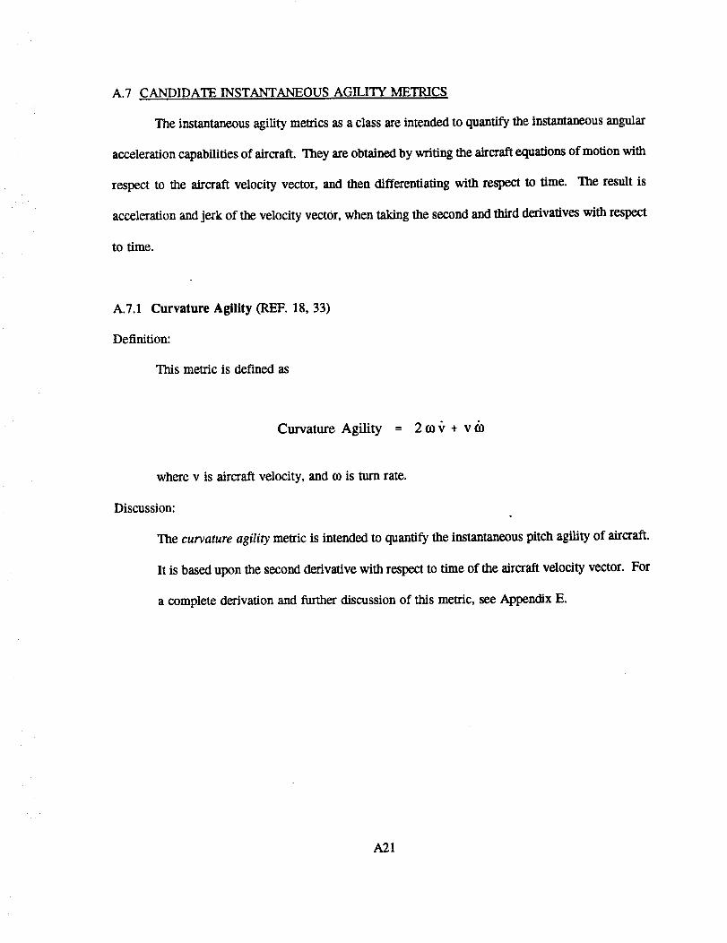
A.7 CANDIDATE INSTANTANEOUS AGILITY METRICS

The instantaneons agility metrics as a class are intended to quantify the instantaneous angular

acceleration capabilities of aircraft. They are obtained by writing the aircraft equations of motion with

respect to the aircraft velocity vector, and then differentiating with respect to time. The result is

acceleration and jerk of the velocity vector, when taking the second and third derivatives with respect

to time.

A.7.1 Curvature Agility (REF. 18, 33)

Definition:

This metric is defined as

Curvature Agility = 2 to _, + v fi_

where v is aircraft velocity, and to is turn rate.

Discussion:

The curvature agility melric is intended to quantify the instantaneous pitch agility of aircraft.

It is based upon the second derivative with respect to time of the aircraft velocity vector. For

a complete derivation and further discussion of this metric, see Appendix E.

A21

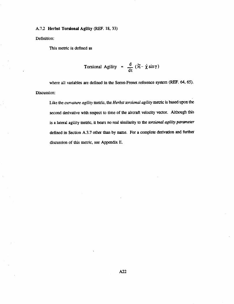
A.7.2 Herbst Torsional Agility (REF. 18, 33)

Definition:

This metricisdefinedas

d zsinr)Torsional Agility --- d'-t"

where allvariablesaredefinedinthe Scrrct-Frenetreferencesystem(REF. 64,65).

Discussion:

Likethecurvatureagilitymetric,theHerbsttorsionalagilitymetricisbasedupon the

secondderivativewithrcspocttotimeof theaircraftvelocityvector.Although this

isa lateralagilitymetric,itbearsno realsimilaritytothetorsionalagilityparameter

definedinSectionA.3.7otherthanby name. For a completederivationand further

discussionof thismetric,see Appendix E.

A22

B. FLIGHT SIMULATION PROGRAMS

B.1 BACKGROUND

This appendix contains descriptions of the flight simulation computer programs used to obtain

the results in this report. The aircraft models consist of a generic F-5A, generic F-16A, generic F-

18A, and generic X-29A. Brief descriptions of the simulation programs, summaries of the mass

properties used for the test cases, and physical descriptions are provided.

B.2 GENERIC F-5A SIX DEGREE-OF-FREEDOM AIRCRAFT SIMULATION (ATHP)

The flight simulation program used to model the generic F-5A Freedom Fighter is the

University of Kansas Flight Research Laboratory's version of the Aircraft Time History Program

(ATHP) (REF. 66). The ATHP simulation is a high fidelity non real-time, nonlinear six degree-of-

freedom aircraft simulation. It contains full flight control system, engine, and aerodynamic models.

The flight control system is representative of the generic F-5A, consisting of pilot command inputs

and a stability augmentation system. The aerodynamic data base contains nonlinear, steady

aerodynamic data for up-and-away flight at angles of attack up to and including 40 °. The aerodynamic

data base was obtained from wind tunnel data. The engine model is nonlinear and is representative

of the F-5A's powerplants. User interface to ATHP is through input and output files. The input flies

contain initial attitude and flight condition, and pilot commands in the form of longitudinal and lateral

stick commands, rudder, and throttle time histories. Output files consist of tabular time history data

which is plotted using standard plotting routines. Any special processing such as filtering or

estimation is performed within the simulation itself when possible. All data collection runs for the

generic F-5A were performed at the following mass properties.

B1

1) Aircraft weight: 12,000 Obf)

2) Inertias: Ixx = 2,620 (slug-_)Iyy = 30,300 (slug-_)

Izz = 32,300 (slug-_)

Ixz = -190 (slug-f_)

The external physical characteristics of the F-5A are displayed in Figure B. 1.

B.3 GENERIC F-16A SIX DEGREE-OF-FREEDOM AIRCRAFT SIMULATION (F-16SIM)

The flight simulation program used to model the generic F-16A Fighting Falcon is the

University of Kansas Hight Research Laboratory's F-16SIM. The F-16SIM simulation is a high

fidelity non real-time, nonlinear six degree-of-freedom aircraft simulation. It contains full flight

control system, engine, and aerodynamic models. The flight control system is representative of the

generic F-16A. The aerodynamic data base contains nonlinear, steady aerodynamic data for up-and-

away flight. The aerodynamic data base was obtained from wind tunnel data. The engine model is

nonlinear and is representative of the F- 16A's powerplant. User interface to F-16SIM is through input

and output files. The input files contain initial attitude and flight condition, and pilot commands in

the form of longitudinal and lateral stick commands, rudder, and throttle time histories. Output files

consist of tabular time history data which is plotted using standard plotting routines. Any special

processing such as filtering or estimation is performed within the simulation itself when possible. All

data collection runs for the generic F-16A were performed at the following mass properties:

B2

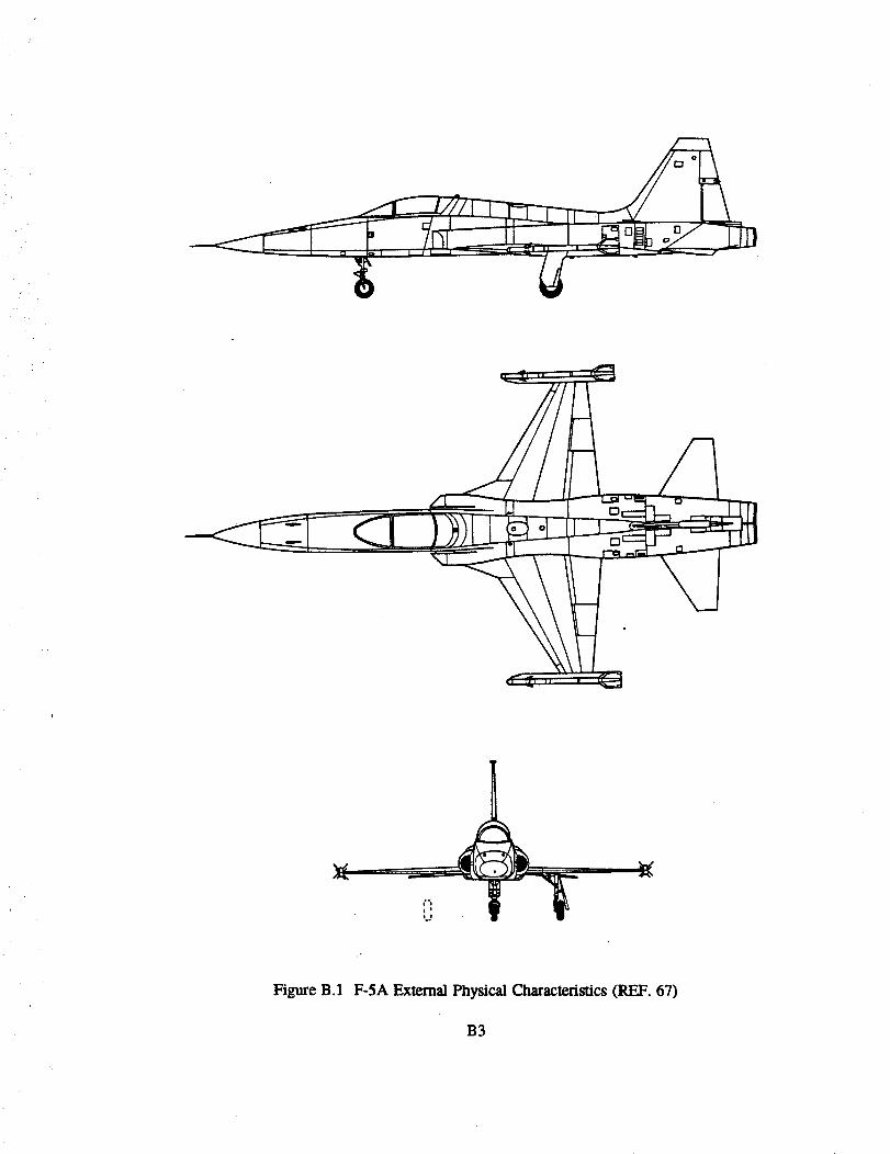
r m I

i"s

I *

i}

Figure B.1 F-5A External Physical Characteristics (REF. 67)

B3

1) Aircraft weight: 20,048 0bf)

2) Inertias: Ixx = 7,035 (slug-f_)

Ivy = 52,372 (slug-H)

Izz = 57,160 (slug-f_)

lxz - 52.2 (slug-H)

3) Center of gravity location: 35.0% MGC

The external physical characteristics of the F-16A are displayed in Figure B.2

B.4 GENERIC F-18A SIX DEGREE-OF-FREEDOM AIRCRAFT SIMULATION (SIM-II)

The generic F-18A Hornet flight simulation computer program is the University of Kansas

Flight Research Laboratory's version of Sim-II (REF. 8). The Sim-II program is a high fidelity, non

real-time, nonlinear six degree-of-freedom aircraft simulation which has been used throughout the

industry to model a wide range of aircraft. It contains full flight control system, engine, and

aerodynamic models. The flight control system model is of version 8.3.3, and runs multi-rate with

gain scheduling. All limiters and nonlinearities in the flight control system are present. The

aerodynamic data base contains nonlinear, steady aerodynamic data for up-and-away flight at angles

of attack up to and including 70 degrees. The aerodynamic data base was obtained from wind tunnel

data and is corrected to flight test data, including flexibility effects. The engine model is nonlinear

and is representative of the F-18A powerplant. User interface to Sim-II is through input and output

files. The input files contain initial attitude and flight cgndition, and pilot commands in the form of

longitudinal and lateral stick position, rudder, and throttle time histories. Output flies consist of

tabular time history data which is plotted using standard plotting routines. Any special processing

such as filtering or estimation is performed within the simulation itself when possible. All simulation

B4

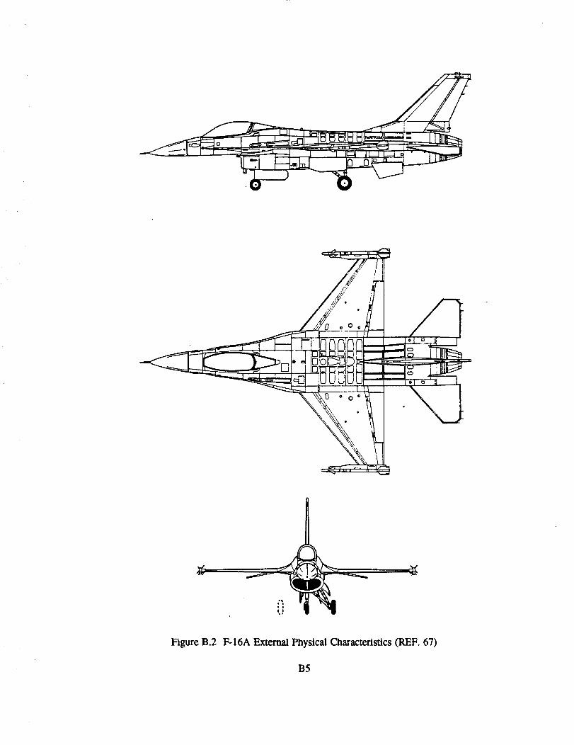
0 o 0 °

o 0 o

Figure B.2 F-16A External Physical Cl_racteristics (REF. 67)

B5

datacollectionnms for the generic F-18A were performed with the following mass properties:

1)

2)

3)

Aircraft weight: 30,540 (lb0

Inertias: Ixx -- 21,957 (slug-_)

Iya, ---122,506 (slug-ft 2)Izz = 137,339 (slug-_)

Ixz -- 1,912 (slug-_)

Center of gravity location: 23.3% MC-CFS 456.17 inches

The external physical characteristics of the F-18A are displayed in Figure B.3.

B.5 GENERIC X-29A SIX DEGREE-OF-FREEDOM AIRCRAFT SIMULATION

The generic X-29A flight simulation computer program at the NASA-Ames Dryden Flight

Research Facility was used to obtain all of the generic X-29A data for this report. All simulation data

collection runs for the generic X-29A were performed with the following mass properties:

1)

2)

3)

Aircraft weight: 15,000 0b0

Inertias: Ixx = 4,600 (slug-_)

Ire = 53,600 (slug-_)

Izz = 56,000 (slug-_)

lxz - 2,500 (slug-f_)

Center of gravity location: between FS 443.5 and 454. inches

The external physical characteristics of the X-29A are displayed in Figure B.4.

B6

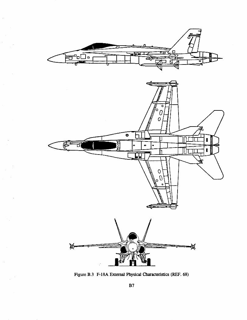
O

Figure B,3 F-18A External Physical Characteristics (REF. 68)

B7

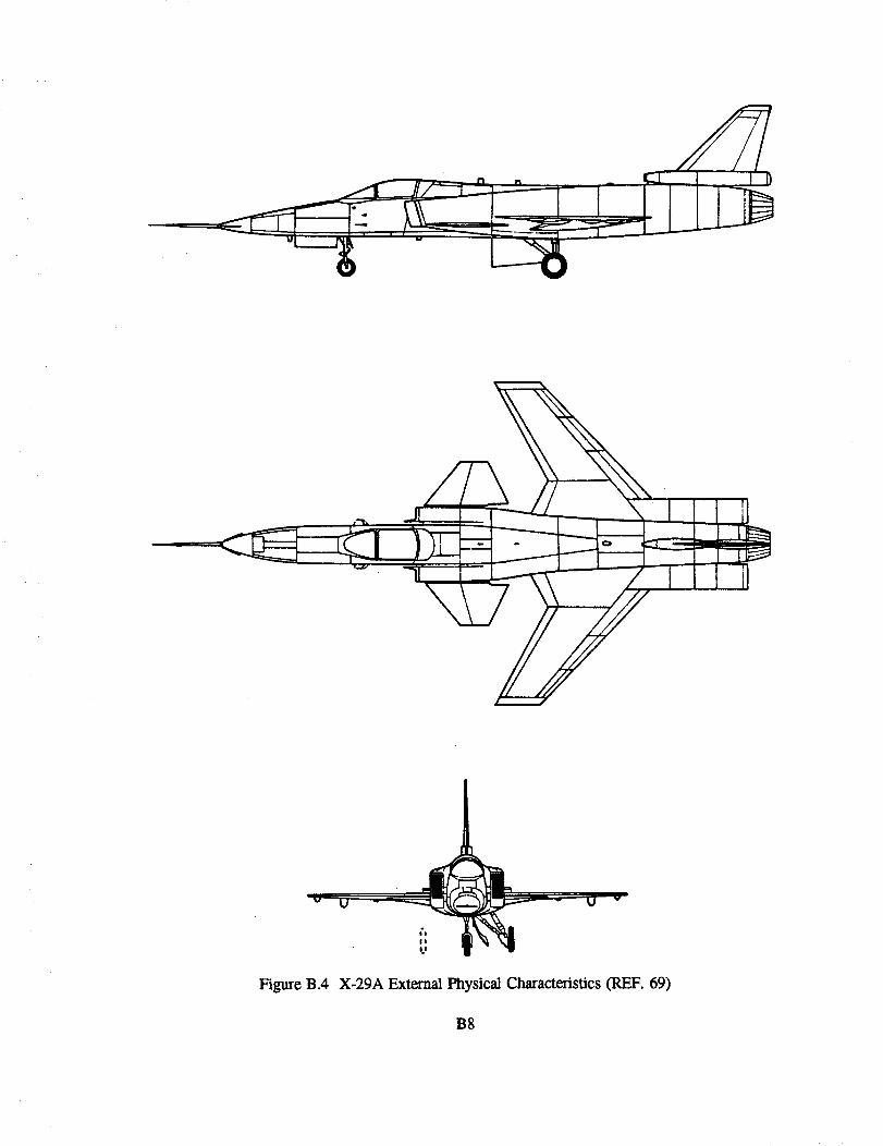
i"1

IQ

Figure B.4 X-29A External Physical Characteristics (REF. 69)

B8

B.6 OPTIMAL TRAJECTORIES BY IMPLICIT SIMULATION PROGRAM (OTIS)

The following description is condensed from Reference 53. OTIS is a general purpose

FORTRAN program for simulating and optimizing point mass trajectories for a wide variety of

aerospace vehicles. The code was written by the Boeing Aerospace and Electronics company in

Seattle, Washington for the Aeronautical Systems Division of the Wright Research and Development

Center (REF. 9, 10). The code consists of over 400 subroutines with a total of over 74000 lines and

can estimate aerodynamic heating for a vehicle and develop propulsion models for the vehicle, in

addition to optimal trajectory development. The OTIS program can be run in one of four different

modes to solve any of the following problems:

1) Generate a discrete trajectory for a set of predefined controls andfixed initial conditions (Mode 1-Explicit Trajectory Integration).

2) Solve targeting problems by varying the values of a set of specified

independent variables to provide a trajectory which passes through a

set of waypoints and/or satisfies preset boundary conditions (Mode2 - Explicit Trajectory Integration With Targeting).

3) Compute an optimal trajectory by varying a set of independent

variables, usually less than 10 in number. Constraints can be

imposed. For optimization, the number of independent variables must

be greater than the number of active constraints. If the number isless, a solution is not possible unless the constraints are dependent in

some way on each other. If the number is equal, a feasible solution

is possible but there is no freedom for optimization (Mode 3 -

Explicit Trajectory Integration With Optimization).

4) Optimize trajectories by generating control functions and varying

discrete parameters. The major difference between this problem and

the previous one is that the optimal control problem has, in theory,an infinite number of degrees of freedom since control functions are

being sought, rather than just discrete parameters. Also, pathconstraints which encompass the entire trajectory can be imposed

(Mode 4 - Implicit Trajectory Optimization).

B9

Theabove problems are complimentary because a discrete trajectory generated using Mode

1 can be used as an input for generating targeting and optimal trajectory solutions in Modes 2-4. In

addition, Mode 1 trajectories can be used to verify the accuracy of Mode 4 results. The above

problems can be solved for a wide variety of vehicles, such as aircraft, missiles, or spacecraft. The

vehicle type os defined by user inputs that are read into the program through a namelist file. The

inputs for the program consist of the following:

1) General inputs to describe the number of phases to divide the

trajectory into, the type of atmospheric model to be used, and what

coordinate system is to be used for integration.

2) Initial conditions and final conditions for trajectory to be simulated.This includes initial conditions for the states and controls and the

starting and ending time constraints to be placed on the trajectory.

3) Constraints to be enforced at every point along the trajectory, such as

limits on load factor, angle of attack, or altitude.

4) Scaling factors to be used to dimension all the states and controls in

the program. This is done to bring all the variables within the same

order of magnitude to allow the program to equally weigh all the

variables in the solution process.

5) Definition of the objective function. This is a combination of any of

the variables within the program, independent or dependent. For

most problems in this thesis, maneuver time was the optimized

parameter.

6) Inputs to describe the vehicle to be modeled, including the numberof engines, the reference areas to be used for aerodynamiccalculations, and the number of stages. Also, a tabular data file is

used to input the aerodynamic and propulsion models for the vehicle.

B10

7) Details of the parameters to be output by the program. This includes

the generation of plots and tabular data files. The routines used in

the code include techniques to convert the objective function to be

minimized into a quadratic approximation, methods to estimate

Lagrange multipliers for the quadratic function, and an algorithm tocalculate the active set of constraints applicable to the problem. Oncethe active set is found and the constraints are determined, the problem

is sent to a nonlinear quadratic programming algorithm to solve for

the states and controls that minimize the objective function.

A sample namelist input file and printout of the tabular data file is available in Reference 53.

Bll

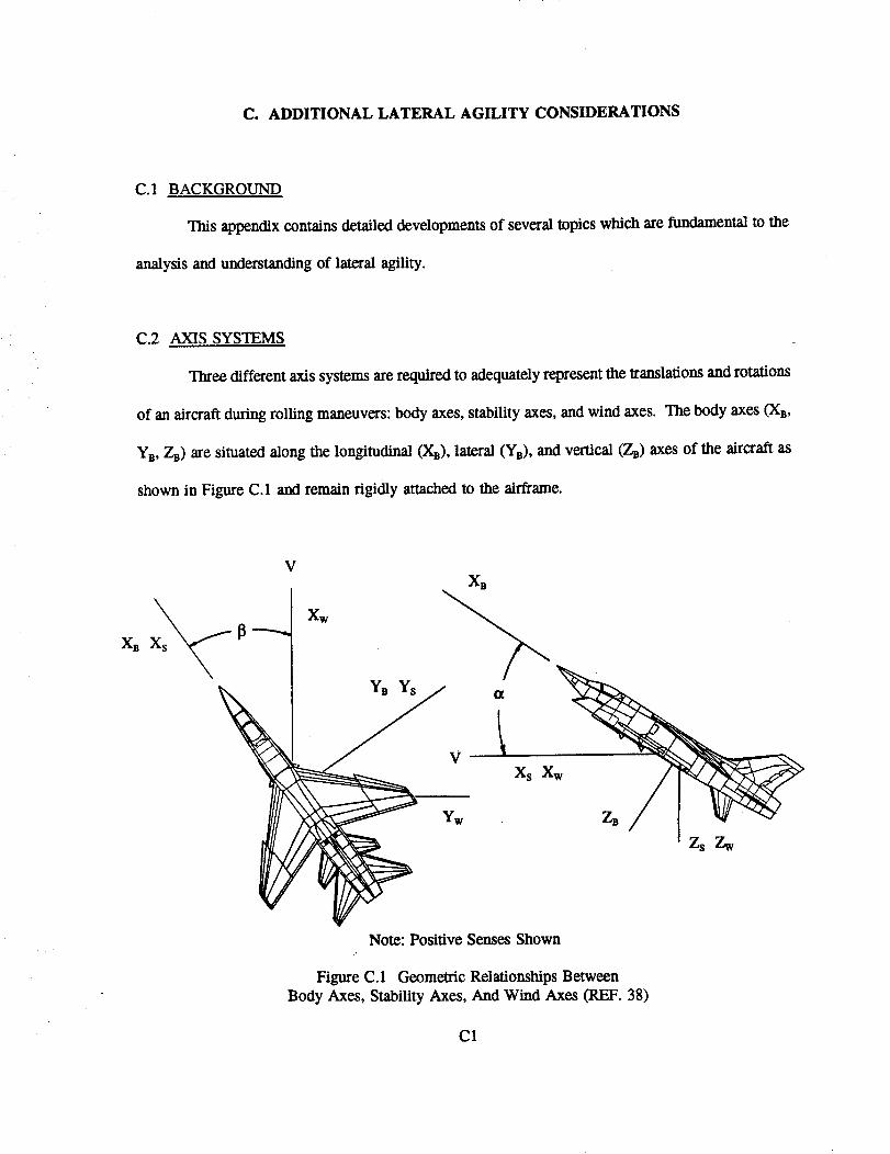
C. ADDITIONAL LATERAL AGILITY CONSIDERATIONS

C.1 BACKGROUND

This appendix contains detailed developments of several topics which are fundamental to the

analysis and understanding of lateral agility.

C.2 AXIS SYSTEMS

Three different axis systems are required to adequately represent the Iranslations and rotations

of an aircraft during rolling maneuvers: body axes, stability axes, and wind axes. The body axes (XB,

YB, Ze) are situated along the longitudinal (Xe), lateral (YB), and vertical (Ze) axes of the aircraft as

shown in Figure C. 1 and remain rigidly attached to the airframe.

XB

VXB

Xw

YB Ys _

'X XNote: Positive Senses Shown

Figure C.1 Geometric Relationships Between

Body Axes, Stability Axes, And Wind Axes (REF. 38)

C1

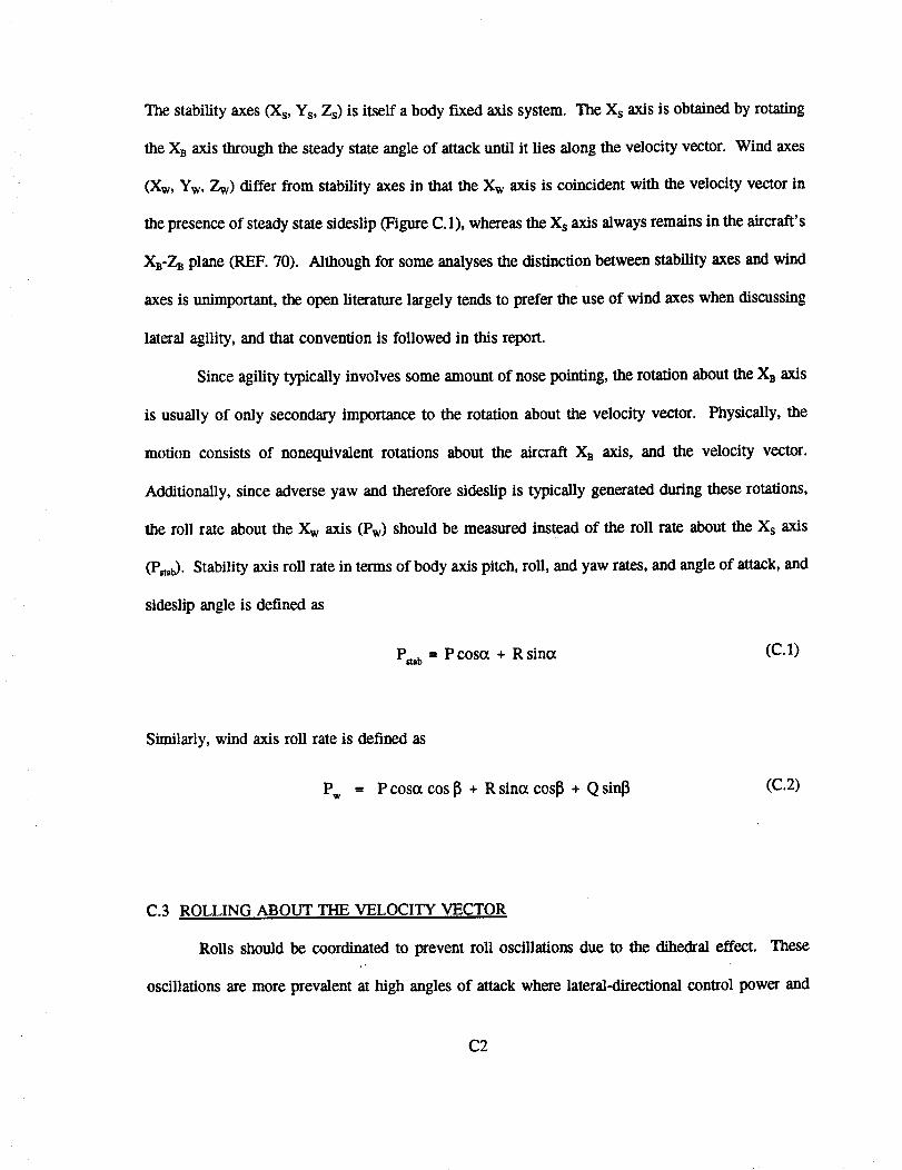
Thestability axes (Xs, Ys, Zs) is itself a body fixed axis system. The Xs axis is obtained by rotating

the XB axis through the steady state angle of attack until it lies along the velocity vector. Wind axes

(Xw, Yw, Zw) differ from stability axes in that the Xw axis is coincident with the velocity vector in

the presence of steady state sideslip (Figure C.1), whereas the Xs axis always remains in the aircraft's

XB-ZB plane (REF. 70). Although for some analyses the distinction between stability axes and wind

axes is unimportant, the open literature largely tends to prefer the use of wind axes when discussing

lateral agility, and that convention is followed in this report.

Since agility typically involves some amount of nose pointing, the rotation about the XB axis

is usually of only secondary importance to the rotation about the velocity vector. Physically, the

motion consists of nonequivalent rotations about the aircraft XB axis, and the velocity vector.

Additionally, since adverse yaw and therefore sideslip is typically generated during these rotations,

the roll rate about the Xw axis (Pw) should be measured instead of the roll rate about the Xs axis

(Pro0. Stability axis roll rate in terms of body axis pitch, roll, and yaw rates, and angle of attack, and

sideslip angle is defined as

Pmb = P cosot ÷ R sinot (C.1)

Similarly, wind axis roll rate is defined as

Pw -- P costx cos _ + R sintx cos_ + Q sin_ (C.2)

C.3 ROLLING ABOUT THE VELOCITY VECTOR

Rolls should be coordinated to prevent roll oscillations due to the dihedral effect. These

oscillations are more prevalent at high angles of attack where lateral-directional control power and

C2

directional stability are reduced. A coordinated roll is defined here as a roll which occurs with zero

sideslip angle. Roll coordination should not be confused with turn coordination, which is defined by

lateral acceleration being equal to zero. Note that while a turn changes the direction of the velocity

vector, a roll rotates the airframe about the velocity vector. The source of nonzero sideslip angles

during a roll can be identified by considering the equation for sideslip rate:

= P sintx - R costx + sinCpcos0 _ + g (C.3)v,

For simplicity, Equation C.3 assumes the sideslip angle to be zero. Equation C.3 is however a good

approximation to the complete equation used by nonlinear six degree-of-freedom aircraft simulations

such as Reference 8 for values of sideslip angle at least as large as those encountered in this research.

This was verified by comparing the sideslip rate from the genetic F-18A simulation to that calculated

by Equation C.3.

Sideslip rate can be divided into kinematic, gravitational and lateral g terms:

_ki_ -- P sina - R cosa(C.4)

gg_" " sin, cos O V-'_

(c.5)

(c.6)g_.mas " ny'_t t

Sideslip due to the kinematic term, called kinematic coupling, occurs when body axis roll and yaw

rates are proportioned such that the axis of airframe rotation is not parallel to the velocity vector. The

other two terms describe the sideslip rate caused by the forces acting on the airplane. During a roll

C3

thesetwotermscannotbeheld to zero. Gravity effects sideslip rate in all attitudes except _ = 0 °,

180 ° and 0 = __90 °, while the control surface deflections required to roll the airplane produce lateral

acceleration. Therefore, in order to roll with sideslip rate equal to zero, there needs to be just enough

kinematic coupling to cancel the effects of gravity and lateral acceleration. To get a general idea of

the body axis roll and yaw rates needed for roll coordination, Equation C.3 is set to zero and the

effects of gravity and lateral g's are neglected:

0 -- P sinct - R cosct (C.7)

Solving for body axis yaw rate,

R = P tano_ (C.8)

Substituting Equation C.8 into Equation C. 1 and multiplying by cos(x, the body axis roll rate (P) can

be expressed as a function of stability axis roll rate (Pmb) and angle of attack as

p .. PmbcosCt (C.9)

Then using Equation C.8, body axis yaw rate can be expressed as

R -- Pmbsinct (C.10)

tEquations C.9 and C.10 are used to construct Figure C.2 which indicates combinations of the body

axis roll rates (P) and yaw rates (R) as a percent of Pa_b which are required at zero sideslip over a

range of angles of attack. Although these are simple relationships, they are important in understanding

the roll and yaw rate requirements for lateral agility, especially at high angles of attack. For example,

in order to be capable of a P,_, of 100 degrees per second at 20 ° angle of attack, a body axis roll rate

of 87 degrees per second, and a body axis yaw rate of 27 degrees per second are required. Although

a 100 degree per second body axis roll rate is typically very easy to achieve for most any jet fighter,

the same fighter may not be able to achieve the same rate of stability and/or wind axis roll. This is

C4

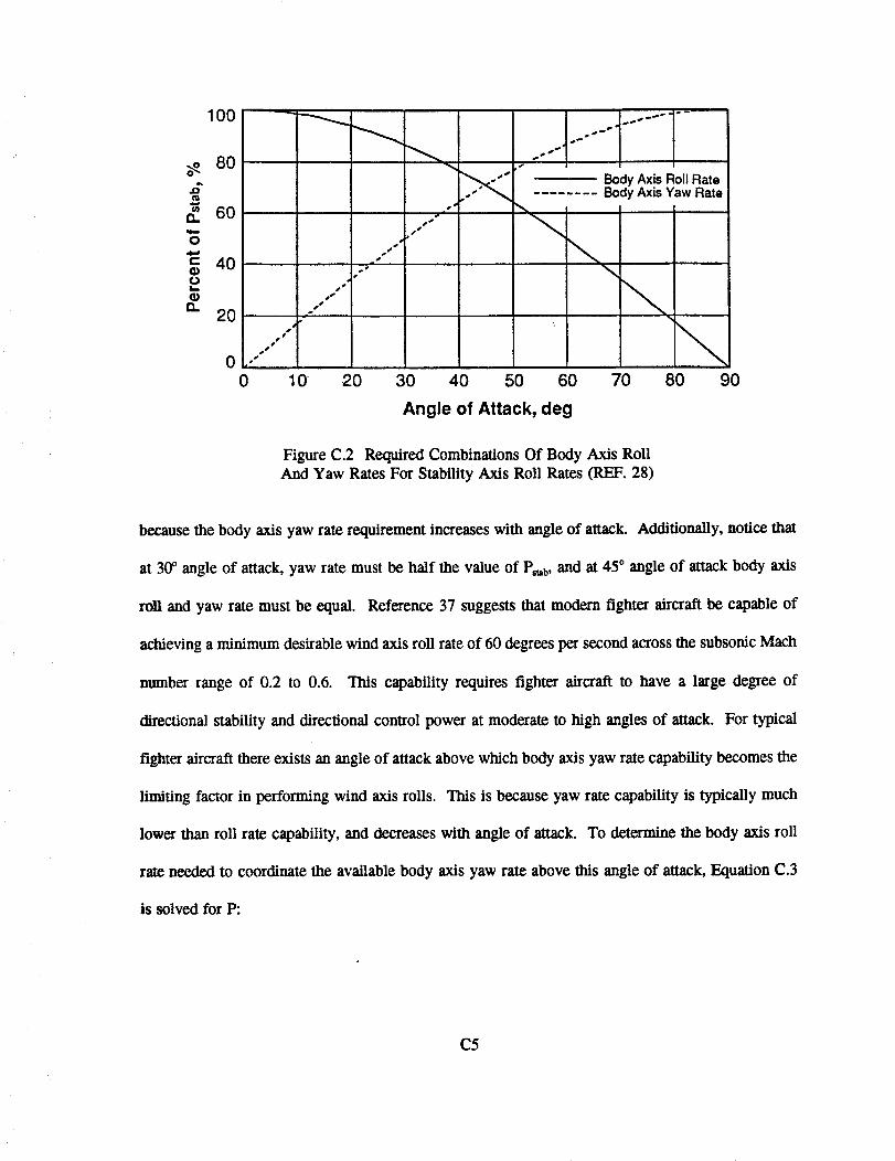
o__t.n

O

e-(Doit..

(I)IX

100 __

8O

6O

4O

s °

sA,

s °

20 -,"o, # •

_,A, •

0

0 10

fL o"

S °

is _S

•* o _

s

20 30 40 50 60

o w

Body Axis Roll RateBody Axis Yaw Rate

\

\70 80 90

Angle of Attack, deg

Figure C.2 Required Combinations Of Body Axis RollAnd Yaw Rates For Stability Axis Roll Rates (REF. 28)

because the body axis yaw rate requirement increases with angle of attack. Additionally, notice that

at 30° angle of attack, yaw rate must be half the value of Pmb, and at 45 ° angle of attack body axis

roll and yaw rate must be equal. Reference 37 suggests that modem fighter aircraft be capable of

achieving a minimum desirable wind axis roll rate of 60 degrees per second across the subsonic Mach

number range of 0.2 to 0.6. This capability requires fighter aircraft to have a large degree of

directional stability and directional control power at moderate to high angles of attack. For typical

fighter aircraft there exists an angle of attack above which body axis yaw rate capability becomes the

limiting factor in performing wind axis rolls. This is because yaw rate capability is typically much

lower than roll rate capability, and decreases with angle of attack. To determine the body axis roll

rate needed to coordinate the available body axis yaw rate above this angle of attack, Equation C.3

is solved for P:

C5

P = Rcoto_ - sin_cos0 g - ny g (C.11)V t sino_ V t sina

Equation C. 11 represents the roll control surface contribution to roll rate which is required to maintain

roll coordination as a function of the available yaw raW. It is important that rolls be coordinated to

avoid oscillations in the lateral-directional axis which tend to reduce controllability. The equations

presented here allow the cause of sideslip during a roll to be isolated and identified.

As an example of roll coordination analysis, consider the generic F-18A response to a full

lateral stick roll at Mach equals 0A at an altitude of 15,000 feet (Figure C.3). Full positive lateral

stick is input at time equals six seconds, while aft stick is held constant at 1.5 inches, which is 30%

of full aft stick deflection. Figure C.3 shows that although the rudders generate a large amount of yaw

rate, they saturate quickly, and adverse sideslip builds up to seven degrees. The cause of the adverse

sideslip can be found by plotting sideslip rate (Equation C.3) along with the three terms for sideslip

rate (Equations C.4, C.5, and C.6). This is done in Figure C.4, which demonstrates that the kinematic

team is dominant. In the first half second, the kinematic term reaches over twice the magnitude

reached by the next largest term, the gravitational term. Plotting the roll rat_ required for coordination

(Equation C.9) with the actual roll rate shows the cause of the kinematic coupling. Figure C.5 shows

that too much roll rate was commanded in the first 1.25 seconds for the amount of yaw rate that was

available. Methods to improve the roll coordination would be in the form of a faster rudder, to allow

the yaw rate to "keep up" with the roll rate; or a reduced roll rate, in proportion to the available yaw

rate. The interested reader should consult Reference 26 for more details on these aspects.

Controlling and maintaining angle of attack is another concern when performing rolls about

the velocity vector. By examining the equation for time rate of change of angle of attack,

C6

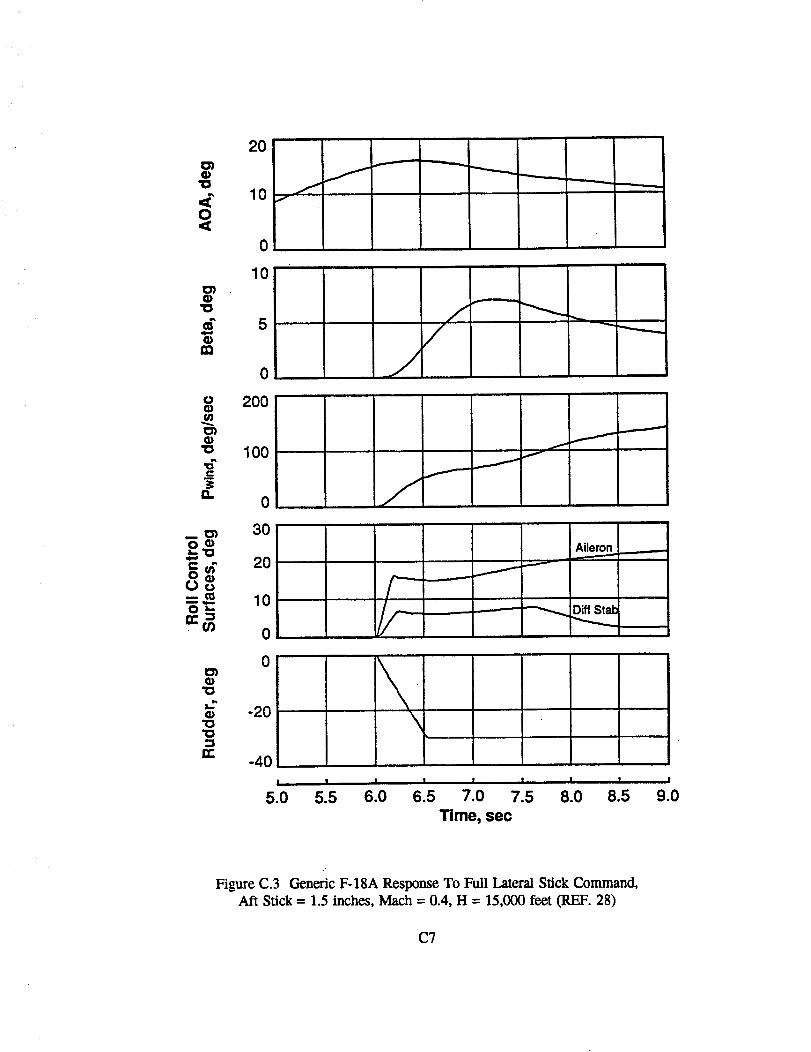
"O

O

1O

¢£G)

m

O

G)1O

3=I%.

,..¢_O_L1O,,$.,,

=,EOom QII.=O"-

03

1O

101O

n-

2O

10

0

10

5

0

200

100

0

30

20

10

0

0

-20

-40

I I I

5.0 5.5 6.0

f_

f

J

f

Aileron

I

--_ Diff Stab

I I I I I

6.5 7.0 7.5 8.0 8.5

Time, sec

!

9.0

Figure C.3 Generic F-18A Response To Full Lateral Stick Command,

Aft SOck = 1.5 inches, Mach = 0.4, H = 15,000 feet (REF. 28)

C7

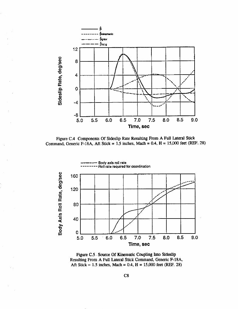
12

O8ol

¢3)O

"O4

mrr

0oum01O"O

-4

-8

5.0 5.5

IT_nq_t_

_rev

_lat g

s o

.,.,.I".,,6.0 6.5 7.0 7.5 8.0 8.5 9.0

Time, sec

Figure C.4 Components Of Sideslip Rate Resulting From A Full Lateral StickCommand, Generic F-18A, Aft Stick = 1.5 inches, Math = 0.4, H = 15,000 feet (REF. 28)

O160

01

"o 120

n-

o 80n,-

¢n

x 40

"00

rn

Body axis roll rateRoll rate required for coordination

0

5.0 5.5

Be"

p.= ,S_

6.0 6.5 7.0 7.5 8.0 8.5 9.0

Time, sec

Figure C.5 Source Of Kinematic Coupling Into Sideslip

Resulting From A Full Lateral Stick Command, Generic F-18A,Aft Stick = 1.5 inches, Mach = 0.4, H = 15,000 feet (REF. 28)

C8

= Q - P+u_tan_ - (L + Tsin(x) gW V, cos D

+(cosO cos(_ cos(x + sin0 sin(x) g

it is seen that there are four contributors:

(C.12)

1. pitch rate

-- Q(C.13)

2. kinematic coupling

_'r_i_ = Pr_tanl3(C.14)

3. lift

_Ii_ = (L + Tsin(x) gW V,cos_

(C.14)

4. gravity

g(cosO cos(_ cos(x + sin0 sin(x)_

v, cosp

(C.15)

Figure C.6 shows an example of how these terms contribute to angle of attack rate for the same full

lateral stick roll maneuver shown in Figure C.3. When the aircraft is rolling, the kinematic coupling

term (Equation C. 13) shows that adverse sideslip contributes a negative value to angle of attack rate.

The lift term (Equation C. 14) remains essentially constant during the maneuver, while the gravitational

term (Equation C.15) switches sign as the aircraft rolls to an inverted attitude. Note that while the

aft stick command was held constant, the flight control system commanded additional pitch rate to

counter the effects of the kinem_c and gravitational terms.

C9

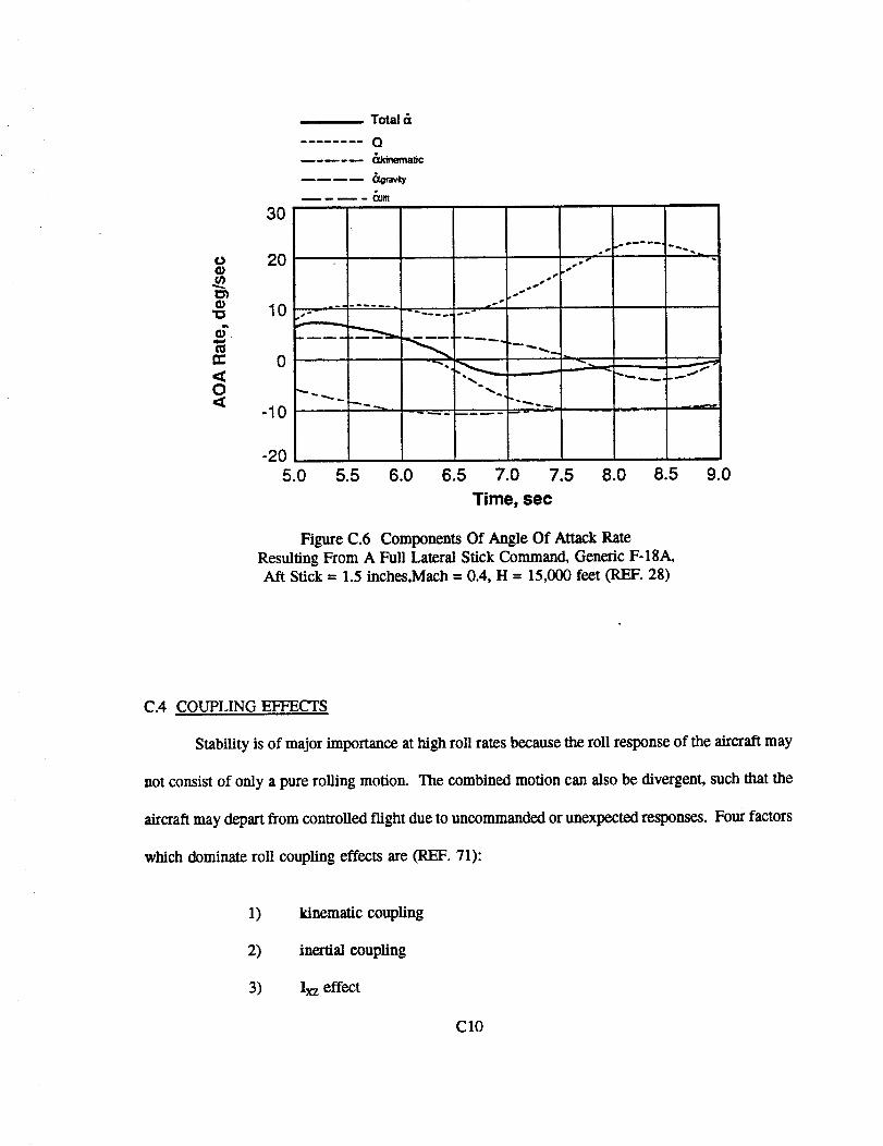
OG)

t_

o"

0

3O

20

10

0

Total &

Q_Udr_ma_c

_w,o

-205.0 5.5 6.0 6.5 7.0 7.5 8.0 8.5

Time, sec

Figure C.6 Components Of Angle Of Attack Rate

Resulting From A Full Lateral Stick Command, Generic F-18A,Aft Stick = 1.5 inches,Mach = 0.4, H = 15,000 feet (REF. 28)

9.0

C.4 COUPLING EFFECTS

Stability is of major importance at high roll rates because the roll response of the aircraft may

not consist of only a pure roiling motion. The combined motion can also be divergent, such that the

aircraft may depart from controlled flight clue to uncommanded or unexpected responses. Four factors

which dominate roll coupling effects are (REF. 71):

1) kinematic coupling

2) inertial coupling

3) Ixz effect

C10

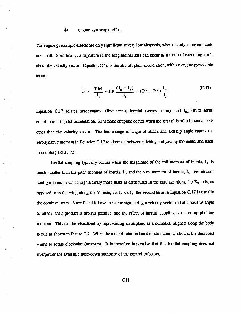
4) engine gyroscopic effect

The engine gyroscopic effects are only significant at very low airspeeds, where aerodynamic moments

are small. Specifically, a departure in the longitudinal axis can occur as a result of executing a roll

Equation C.16 is the aircraft pitch acceleration, without engine gyroscopicabout the velocity vector.

terms.

= Y.M _ PR (Ix - Iz) - (p2 _ R 2) IxzI--:- ly "_y

(C.17)

Equation C.17 relates aerodynamic (firm term), inertial (second term), and Ixz (third term)

contributions to pitch acceleration. Kinematic coupling occurs when the aircraft is rolled about an axis

other than the velocity vector. The interchange of angle of attack and sideslip angle causes the

aerodynamic moment in Equation C.17 to alternate between pitching and yawing moments, and leads

to coupling (REF. 72).

Inertial coupling typically occurs when the magnitude of the roll moment of inertia, Ix, is

much smaller than the pitch moment of inertia, Iv, and the yaw moment of inertia, Iz. For aircraft

configurations in which significantly more mass is distributed in the fuselage along the X B axis, as

opposed to in the wing along the YB axis, i.e. Ix << Iy, the second term in Equation C.17 is usually

the dominant term. Since P and R have the same sign during a velocity vector roll at a positive angle

of attack, their product is always positive, and the effect of inertial coupling is a nose-up pitching

moment. This can be visualized by representing an airplane as a dumbbell aligned along the body

x-axis as shown in Figure C.7. When the axis of rotation has the orientation as shown, the dumbbell

wants to rotate clockwise (nose-up). It is therefore imperative that this inertial coupling does not

overpower the available nose-clown authority of the control effectors.

Cll

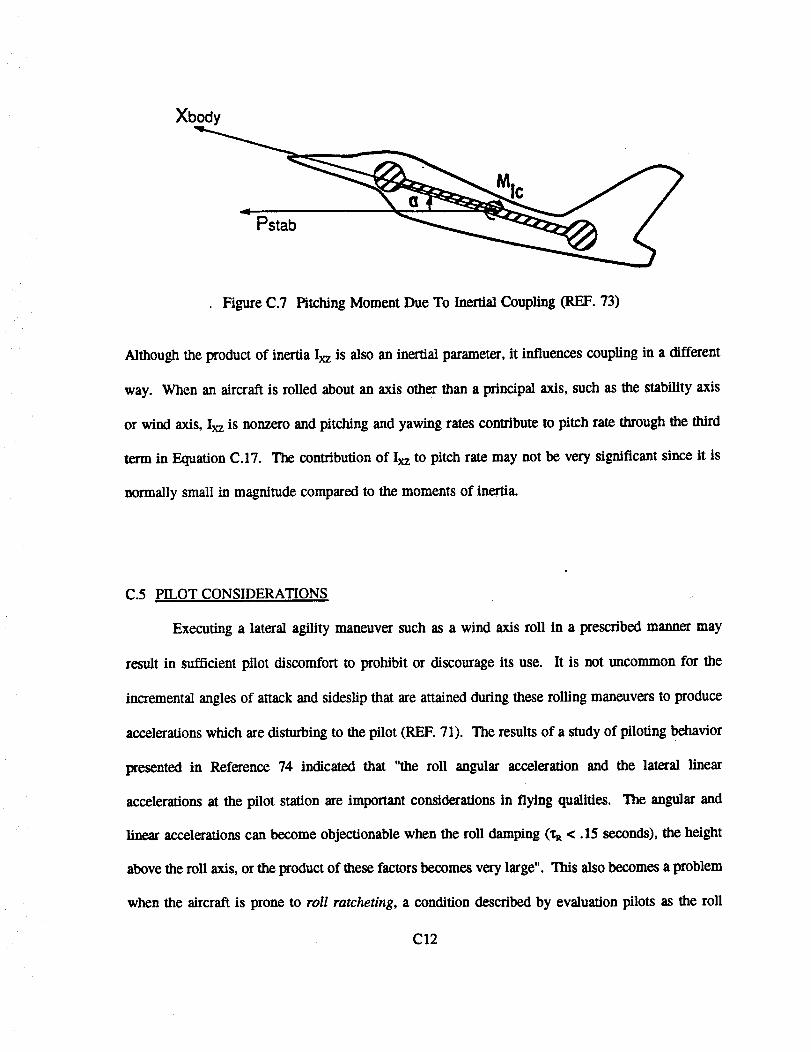
Xbody

Pstab

Figure C.7 Pitching Moment Due To Inertial Coupling (REF. 73)

Although the product of inertia Ixz is also an inertial parameter, it influences coupling in a different

way. When an aircraft is rolled about an axis other than a principal axis, such as the stability axis

or wind axis, Ixz is nonzero and pitching and yawing rates conlribute to pitch rate through the third

term in Equation C.17. Tbe contribution of Ixz to pitch rate may not be very significant since it is

normally small in magnitude compared to the moments of inertia.

C.5 PILOT CONSIDERATIONS

Executing a lateral agility maneuver such as a wind axis roll in a prescribed manner may

result in sufficient pilot discomfort to prohibit or discourage its use. It is not uncommon for the

incremental angles of attack and sideslip that are attained during these rolling maneuvers to produce

accelerations which are disturbing to the pilot (REF. 71). The results of a study of piloting behavior

presentedin Reference 74 indicatedthat "the rollangularaccelerationand the laterallinear

accelerationsatthe pilotstationarc importantconsiderationsin flyingqualities.The angularand

linearaccelerationscan become objectionablewben therolldamping (_R< .15 seconds),theheight

above therollaxis,ortheproductofthesefactorsbecomes verylarge".This alsobecomes aproblem

when the aircraftisprone to rollratcheting,a conditiondescribedby evaluationpilotsas the roll

C12

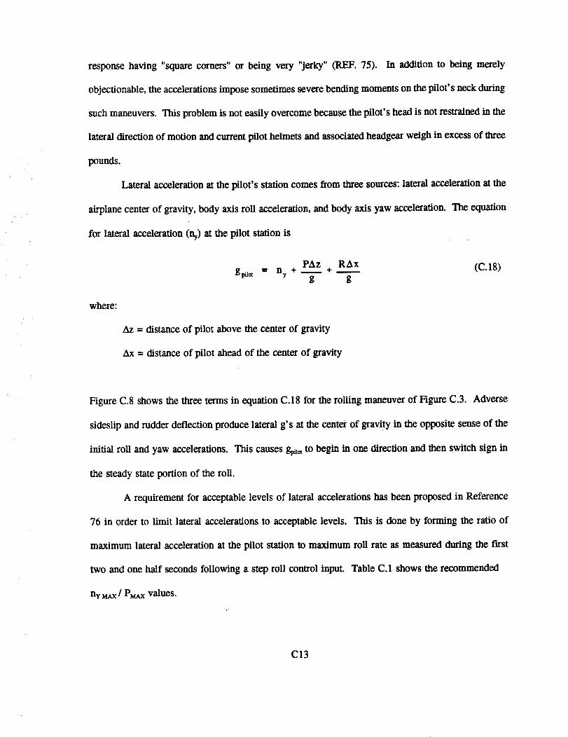
response having "square corners" or being very "jerky" (REF. 75). In addition to being merely

objectionable, the accelerations impose sometimes severe bending moments on the pilot's neck during

such maneuvers. This problem is not easily overcome because the pilot's head is not restrained in the

lateral direction of motion and current pilot helmets and associated headgear weigh in excess of three

pounds.

Lateral acceleration at the pilot's station comes from three sources: lateral acceleration at the

airplane center of gravity, body axis roll acceleration, and body axis yaw acceleration. The equation

for lateral acceleration (ny) at the pilot station is

PAz RAx (C.18)gpflot 'P ny + _ +

g g

where:

Az = distance of pilot above the center of gravity

Ax = distance of pilot ahead of the center of gravity

Figure C.8 shows the three terms in equation C.18 for the rolling maneuver of Figure C.3. Adverse

sideslip and rudder deflection produce lateral g' s at the center of gravity in the opposite sense of the

initial roll and yaw accelerations. This causes gp_,_to begin in one direction and then switch sign in

the steady state portion of the roll.

A requirement for acceptable levels of lateral accelerations has been proposed in Reference

76 in order to limit lateral accelerations to acceptable levels. This is done by forming the ratio of

maximum lateral acceleration at the pilot station to maximum roll rate as measured during the first

two and one half seconds following a step roll control input. Table C.1 shows the recommended

nv MAX/ PM_X values.

C13

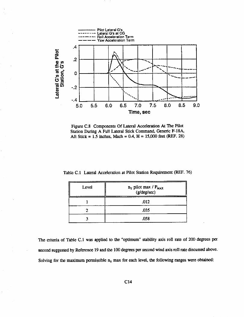
oo_

(*e"ou

L_

II}(I1,.1

.4

.2

0

-.2

Pilot Lateral G'sLateral G's at CGRoll Acceleration TermYaw Acceleration Term

_",t = r

6.0 6.5 7.0 7.5 8.0 8.5 9.0

Time, sec

Figure C.8 Components Of Lateral Acceleration At The PilotStation During A Full Lateral Stick Command, Generic F-18A,Aft Stick = 1.5 inches, Math = 0.4, H = 15,000 feet (REF. 28)

Table C. 1 Lateral Acceleration at Pilot Station Requirement (REF. 76)

Level nv pilot max / P_u,x

(g/deg/sec)

1 .012

2 .035

3 .058

The criteria of Table C.1 was applied to the "optimum" stability axis roll rate of 200 degree, s per

second suggested by Reference 19 and the 100 degrees per second wind axis roll rate discussed above.

Solving for the maximum permissible nv max for each level, the following ranges were obtained:

C14

Level 100 deg/sec 200 deg/sec

1 ny _< 1.2 nv ---2.4

2 1.2 < ny _< 3.5 2.4 < lay _<7.0

3 5.8 < ny 7.0 < ny

The Level 1 ny values for both the 1130and 200 degree per second roll rates appear to be reasonable

when compared with the levels contained in Reference 77. The Level 2 values are arguably

acceptable for the 100 degree per second roll rate since exposure to ny of up to 5g for short durations

impairs but not does not prohibit pilot tracking tasks. The respective values for the 200 degree per

second roll rate would have to be of very short duration if impairment of tracking tasks and ill effects

on the pilot are to be avoided. The Level 3 values are unacceptably high for even extremely short

durations. As a result, it appears that an applicable requirement for lateral accelerations at the pilot

station will need to account for duration of exposure in addition to maximum acceleration levels.

Since lateral agility typically comprise rolling motions at elevated normal load factors, the

possibility of g induced loss of consciousness (GLOC) clue to large lateral accelerations at the pilot

station is a concern. The consideration of large lateral accelerations is important not only for the

determination of flying qualities, but also because of degrading effects on pilot motor and cognitive

performances for demanding tasks such as air-to-air tracking during combat.

Recent research demonstrates that the physiological effect of high lateral accelerations (ny >

2.0) on pilot mission effectiveness is a function of both the magnitude of the imposed acceleration and

the duration of the exposure (REF. 77). Table C.2 indicates the levels of physiological impairment

and effects on pilot mission effectiveness as a result of imposed high lateral accelerations during an

air-to-air combat tracking task.

C15

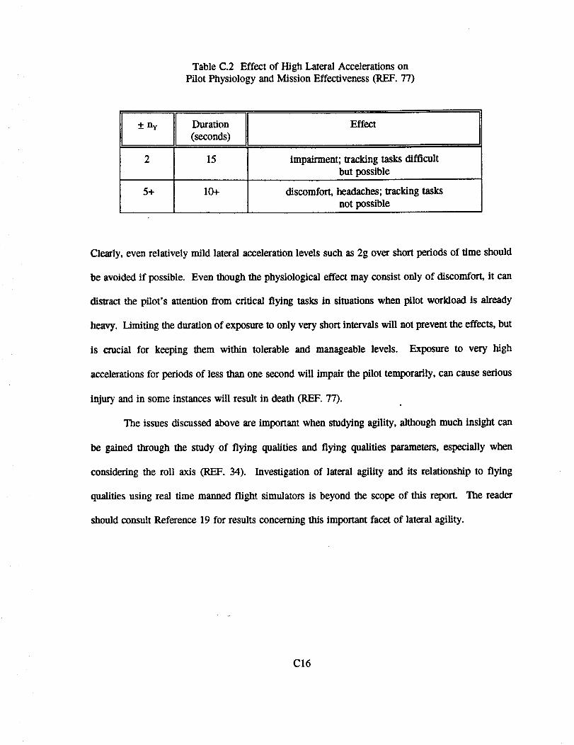
Table C.2 Effect of High Lateral Accelerations on

Pilot Physiology and Mission Effectiveness (REF. 77)

+ny

5+

Duration Effect

(seconds)

15

10+

impairment; tracking tasks difficult

but possible

discomfort, headaches; tracking tasks

not possible

Clearly, even relatively mild lateral acceleration levels such as 2g over short periods of time should

be avoided if possible. Even though the physiological effect may consist only of discomfort, it can

distract the pilot's attention from critical flying tasks in situations when pilot workload is already

heavy. Limiting the duration of exposure to only very short intervals will not prevent the effects, but

is crucial for keeping them within tolerable and manageable levels. Exposure to very high

accelerations for periods of less than one second will impair the pilot temporarily, can cause serious

injury and in some instances will result in death (REF. 77).

The issues discussed above are important when studying agility, although much insight can

be gained through the study of flying qualities and flying qualities parameters, especially when

considering the roll axis (REF. 34). Investigation of lateral agility and its relationship to flying

qualities using real time manned flight simulators is beyond the scope of this report. The reader

should consult Reference 19 for results concerning this important facet of lateral agility.

C16

D. ADDITIONAL AXIAL AGILITY CONSIDERATIONS

D.1 BACKGROUND

A prevalent misconception concerning axial agility is that the axial agility metrics quantify

the level acceleration/deceleration capability of aircraft. This appendix contains an analysis that

elucidates the distinct differences between level acceleration capability and axial agility. An

example result is presented using the genetic F-18A.

D.2 THE COMPONENTS OF AXIAL AGILITY

Axial agility metrics do not quantify the acceleration or deceleration performance of an

aircraft. This can be shown by starting with the relation for specific excess power (REF. 78)

V(T-D) (D.1)Ps = W

where

V = total velocity (ft/sec)T = thrust (lbf)

D = drag 0bf)W = weight (lbf)

Since AP s/At is approximately the derivative of Ps with respect to time, Equation D.1 is

differentiated to obtain

ot:I'T°'Iot (VlOO ,o2 where the weight is assumed" to be constant. The first term in Equation D.2 is the component of

D1

AP_/At clue to acceleration of the airframe; the second and third terms are the components clue to

time rate of change of thrust and drag respectively. Acceleration (dV/dt) does not have a

pronounced effect on the values of AP,/At. This is because the very short spool times of fighter

aircraft engines (generally between three and five seconds), and the rapid drag rise due to

deployment of speedbrakes cause the time rate of change of the thrust and drag terms to be much

larger than the acceleration term. As a result the second and third terms in Equation D.2 achieve

their respective maximum/minimum values before acceleration becomes large enough to contribute

significantly to AP, IAt. Tlaese relationships are displayed in Figure D.1, which is a plot of the

three terms in Equation D.2 during a typical data collection run. Note that each term is plotted

on a different scale.

The time history of the first term, the contribution of the time rate of change of velocity,

is considerably smaller in magnitude relative to the second and third terms (lime rate of change

of thrust and drag respectively). This demonstrates that axial agility is not dominated by

acceleration capability. The time history of the second term shows the thrust level increasing at

a constant rate from time equals 8.3 seconds to 10.3 seconds, during'the engine spool up time,

before leveling off at maximum thrust. The time rate of change of drag, the third term, reflects

the change (decrease) in drag clue to retraction of the speedbrake over a period of one second,

starting at time equals eight seconds. This time history is less intuitive at first glance due to the

sign convention. When retracting the speedbrake, the time rate of change of drag increases in

magnitude, but is negalJve in sign (since drag is decreasing).

The axial agility of a fighter is also affected by the engine's transient performance during

large scale maneuvering, and at elevated angles of attack and sideslip. Although this engine

behavior is an important contributor to overall combat effectiveness, the power onset parameter

and the power loss parameter do not address this aspect.

D2

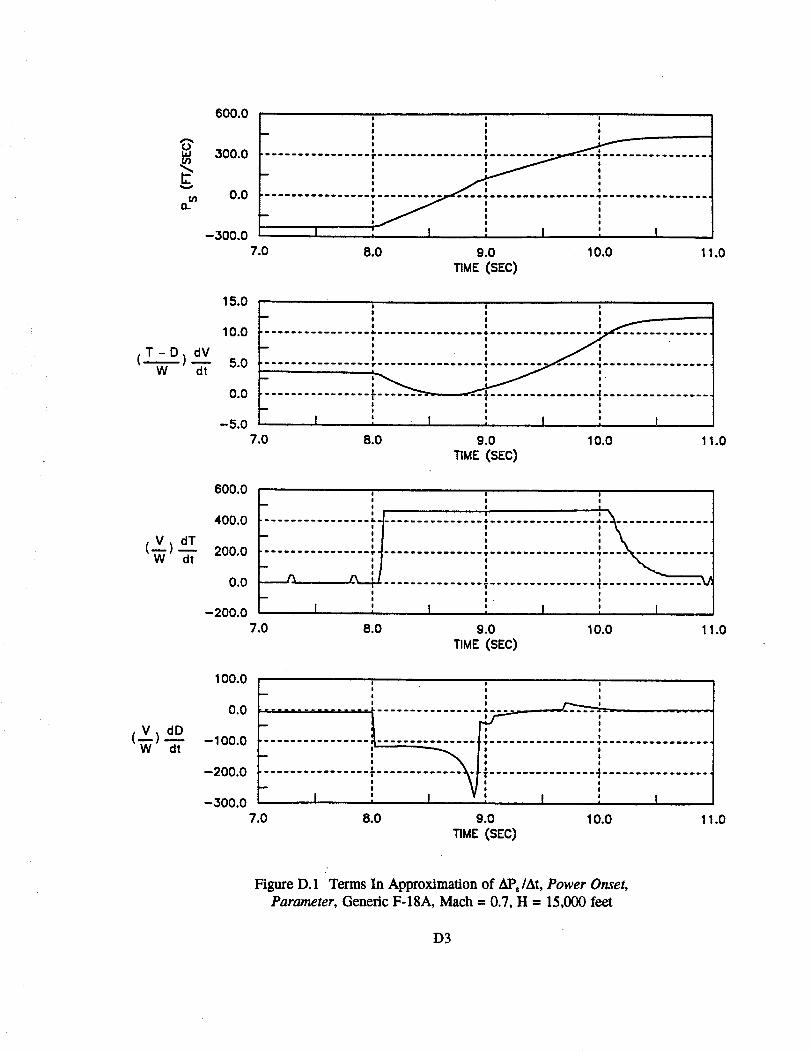
600.0

15.0

J ! !

10.0 ....................................................................!

B I I

T-D) _dV ,, ,'( W dt 5.0 ................. r,................................ _,.................

I I

0.0 .........................! I !

-- ! | 0

-5.0 I : I ', I : I

7.0 8.0 9.0 10.0 1 1.0

TIME (SEC)

600.0

400.0

200.0

0.0

-200.0

Bt

1 I o__ ! |

! ! 0

! ! I

I ! !

-- I I I

_-4 ' °. ! S

!-- I I I

I , I , ! : I

7.o 8.o 9.0 lO.O 11.oTIME (SEC)

(v) dDW dt

100.0

0.0

-100.0

-200.0

-300.07.0

= , !

.................... .. ..... ......_ ..............! !

$ I

• ...............m ......=..==...= ===================================

! I

I I I

I I I.....0...0_....

I I i

8.o 9.o 1o.o 1_.o_ME (SEC)

Figure D. 1 Terms In Approximation of AP,/At, Power Onset,

Parameter, Generic F-18A, Mach= 0.7, H = 15,000 feet

D3

E. DERIVATION OF INSTANTANEOUS AGILITY METRICS

E.1 BACKGROUND

Instantaneous agility is concerned with the instantaneous angular acceleration capabilities

of aircraft. The candidate instantaneous agility metrics are obtained by writing the aircraft

equations of motion with respect to the aircraft velocity vector and then differentiating with

respect to time. The result is acceleration and jerk of the velocity vector, when taking the second

and third derivatives with respect to time. While the derivations of these metrics have remained

proprietary and unpublished in the open literature, the metrics themselves have been published.

The purpose of this chapter is to clearly demonstrate the derivation of these metrics, derive

approximations to the metrics which aid in their physical understanding, and outline the scope of

their applicability.

E.2 CANDIDATE INSTANTANEOUS AGILITY METRICS

E.2.1 Curvature Agility (REF. 18, 33)

Definition:

This metric is defined as

Curvature Agility ffi 2 03x, + v tb

where v is aircraft velocity, and to is turn rate.

Discussion:

The curvature agility metric is intended to quantify the instantaneous pitch agility of

aircraft. It is based upon the second derivative with respect to time of the aircraft velocity

E1

vector. This metric is not task oriented but rather an essentially open loop metric, since

there is no specified initial or terminal state, nor any upper or lower limit on it's value.

E.2.2 Herbst Torsional Agility (REF. 18, 33)

Definition:

This metric is defined as

Torsional Agility -- md( __ Z siny)dt

where the variables are defined in the Serret-Frenet reference system of References 64 and

65:

_/ = pitch angle (or flight path angle)

Z = heading angle= roll angle

Like the curvature agility metric, Herbst torsional agility is open loop and based upon the second

derivative with respect to time of the aircraft velocity vector. Although this is a lateral agility

metric, it bears no real similarity to the torsional agility parameter defined in Section A.3.7 of

Appendix A other than by name.

E.3 DERIVATION AND APPROXIMATION TO THE INSTANTANEOUS AGILITY

METRICS

The Serret-Frenet reference system is briefly introduced to make clear the physical

meaning of the terms in the Herbst torsional agility metric. The pitch angle (or flight path angle)

1" and heading angle Z of the Serret-Frenet system are identical to -/and _ respectively in the

E2

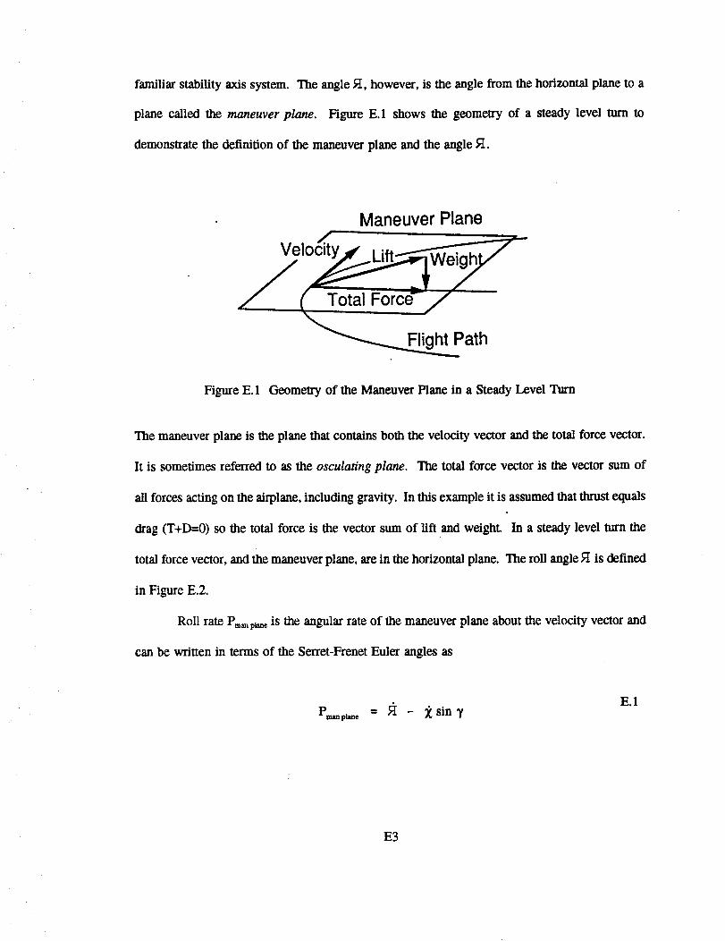
familiarstability axis system. The angle I;t, however, is the angle from the horizontal plane to a

plane called the maneuver plane. Figure E.1 shows the geometry of a steady level turn to

demonstrate the definition of the maneuver plane and the angle _.

./Velocity

Maneuver Plane

Total Force

,ht Path

Figure E. 1 Geometry of the Maneuver Plane in a Steady Level Turn

The maneuver plane is the plane that contains both the velocity vector and the total force vector.

It is sometimes referred to as the osculating plane. The total force vector is the vector sum of

all forces acting on the airplane, including gravity. In this example it is assumed that thrust equals

drag (T+D=-0) so the total force is the vector sum of lift and weight. In a steady level turn the

total force vector, and the maneuver plane, are in the horizontal plane. The roll angle _t is defined

in Figure E.2.

Roll rate Pm_ p_e is the angular rate of the maneuver plane about the velocity vector and

can be written in terms of the Serret-Frenet Euler angles as

Pmnplme -- _ - _ sin yE.1

E3

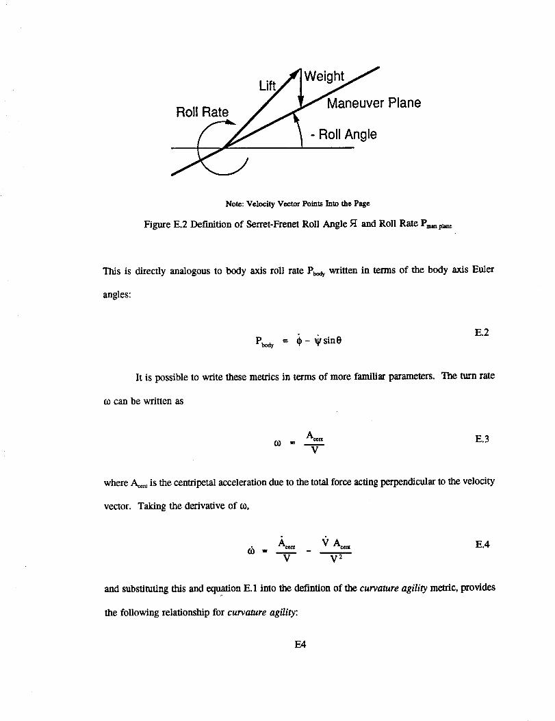
Lift_We_

Roll Rate/_ Maneuver Plane

__/'/ _-RollAngle

Note: Velocity VectorPoints Into the Page

Figure E.2 Definition of Serret-Frenet Roll Angle _ and Roll Rate P=sn pk_r_

This is directly analogous to body axis roll rate P_,oy written in terms of the body axis Euler

angles:

Pbody = 0- _sineE.2

It is possible to write these metrics in terms of more familiar parameters. The turn rate

to can be written as

to A== E.3

V

where A_r_ is the centripetal acceleration due to the total force acting perpendicular to the velocity

vector. Taking the derivative of to,

d_V V _

E.4

and substituting this and equation E.1 into the defintion of the curvature agility metric, provides

the following relationship for curvature agility:

E4

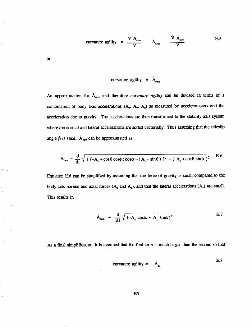
curvature agility_/A_m V A_ E.5

----- ÷ Accnt -V V

or

curvatureagility-- A"m

An approximation for A_m and therefore curvature agility can be devised in terms of a

combination of body axis accelerations (A_, Ay, Az) as measured by accelerometers and the

acceleration clue m gravity. The accelerations are then lransformed to the stability axis system

where the normal and lateral accelerations are added vectorially. Thus assuming that the sideslip

angle 13is small, ,h,,_m can be approximated as

dA=m = -_" _ [ (-An +cosOcos_)cosa-(Ax-sin0) ]: + ( Ay +cosO sin_ ): E.6

Equation E.6 can be simplified by assuming that the force of graviW, is small compared to the

body axis normal and axial forces (A_ and A0, and that the lateral accelerations (A_) are small.

This results in

d _ (_An COS0_ - A sinct):E.7

As a final simplification, it is assumed that the first term is much larger than the second so that

curvatureagility= - ,_,,E.8

E5

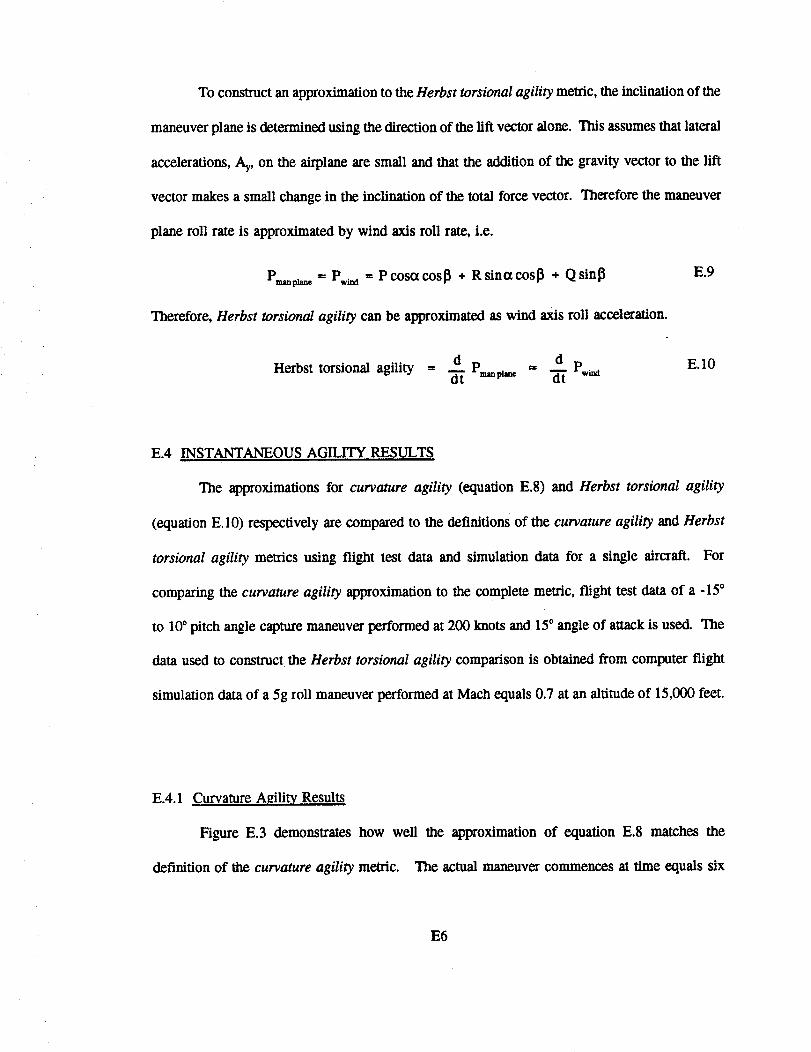
To construct an approximation to the Herbst torsional agility metric, the inclination of the

maneuver plane is determined using the direction of the lift vector alone. Tiffs assumes that lateral

accelerations, Ay, on the airplane are small and that the addition of the gravity vector to the lift

vector makes a small change in the inclination of the total force vector. Therefore the maneuver

plane roll rate is approximated by wind axis roll rate, i.e.

P_pmc _ Pwt_ ---Pcosctcosl 3 ÷ Rsinctcosl3 ÷ Qsinl3

Therefore, Herbst torsional agility can be approximated as wind axis roll acceleration.

d pmanpm_ d P,,t_Herbst torsional agility = ._ =

E.9

E.10

E.4 INSTANTANEOUS AGILITY RESULTS

The approximatiom for curvature agility (equation E.8) and Herbst torsional agility

(equation E.10) respectively are compared to the definitions of the curvature agility and Herbst

torsional agility metrics using flight test data and simulation data for a single aircraft. For

comparing the curvature agility approximation to the complete metric, flight test data of a -15 °

to 10° pitch angle capture maneuver performed at 200 knots and 15° angle of attack is used. The

data used to construct the Herbst torsional agility comparison is obtained from computer flight

simulation data of a 5g roll maneuver performed at Mach equals 0.7 at an altitude of 15,000 feet.

E.4.1 Curvature Agility Results

Figure E.3 demonstrates how well the approximation of equation E.8 matches the

definition of the curvature agility metric. The actual maneuver commences at time equals six

E6

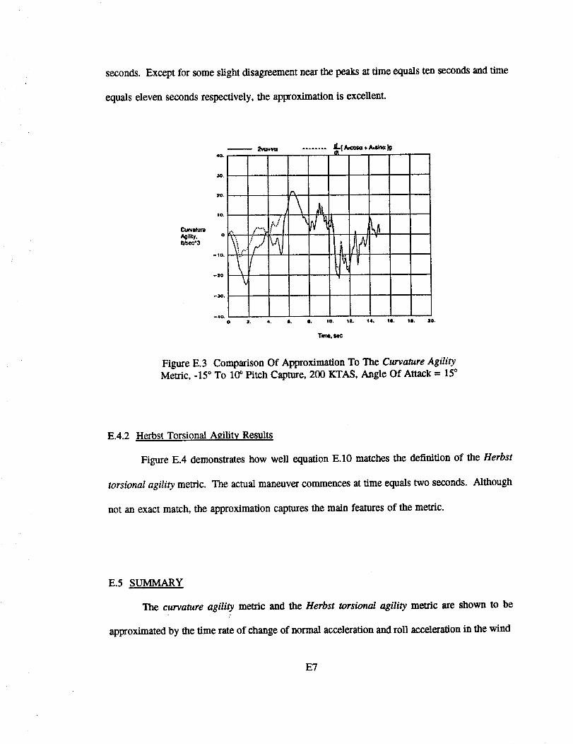
seconds. Except for some slight disagreement near the peaks at time equals ten seconds and time

equals eleven seconds respectively, the approximation is excellent.

I_valum

Agility.

_3

2v_w ........ _ ÷A_na lg

40. -.

2o. t'_

,o. .: _^,_. _', i".., ,,. IV _' I

)..,r"/ i/It '_,o.il v--20

--40,O Z. 4. 6. 8. 10. 12. 14.

TMle. M¢

11, II. lO.

Figure E.3 Comparison Of Approximation To The Curvature AgilityMetric, -15 ° To 10° Pitch Capture, 200 KTAS, Angle Of Attack = 15°

E.4.2 Herbst Torsional Agility Results

Figure E.4 demonstrates how well equation E.10 matches the definition of the Herbst

torsional agility metric. The actual maneuver commences at time equals two seconds. Although

not an exact match, the approximation captures the main features of the metric.

E.5 SUMMARY

The curvature agility metric and the Herbst torsional agility metric are shown to be

approximated by the time rate of change of normal acceleration and roll acceleration in the wind

E7

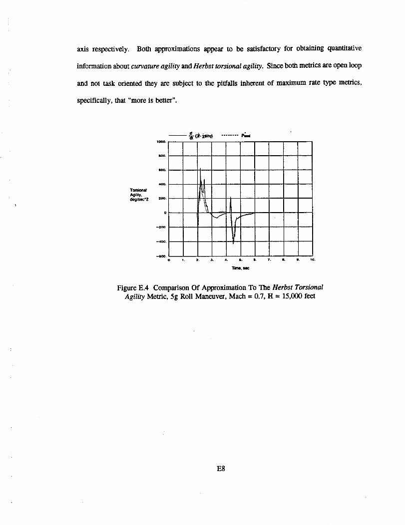
axis respectively. Both approximations appear to be satisfactory for obtaining quantitative

information about curvature agility and Herbst torsional agility. Since both metrics are open loop

and not task oriented they are subject to the pitfalls inherent of maximum rate type metrics,

specifically, that "more is better".

TorsionalAgility.,:_m,c,2

10o0.

eoo.

600.

400.

200.

0

-200

40O

.-ilO0.0

,I

\

I. 2. 3. 4. 7. II. 9. 10.

Figure E.4 Comparison Of Approximation To The Herbst Torsional

Agility Metric, 5g Roll Maneuver, Mach= 0.7, H = 15,000 feet

E8