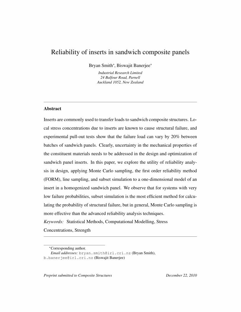
Reliability of inserts in sandwich composite panels

Bryan Smith∗, Biswajit Banerjee∗

Industrial Research Limited24 Balfour Road, Parnell

Auckland 1052, New Zealand

Abstract

Inserts are commonly used to transfer loads to sandwich composite structures. Lo-

cal stress concentrations due to inserts are known to cause structural failure, and

experimental pull-out tests show that the failure load can vary by 20% between

batches of sandwich panels. Clearly, uncertainty in the mechanical properties of

the constituent materials needs to be addressed in the design and optimization of

sandwich panel inserts. In this paper, we explore the utility of reliability analy-

sis in design, applying Monte Carlo sampling, the first order reliability method

(FORM), line sampling, and subset simulation to a one-dimensional model of an

insert in a homogenized sandwich panel. We observe that for systems with very

low failure probabilities, subset simulation is the most efficient method for calcu-

lating the probability of structural failure, but in general, Monte Carlo sampling is

more effective than the advanced reliability analysis techniques.

Keywords: Statistical Methods, Computational Modelling, Stress

Concentrations, Strength

∗Corresponding author.Email addresses: bryan.smith@irl.cri.nz (Bryan Smith),

b.banerjee@irl.cri.nz (Biswajit Banerjee)

Preprint submitted to Composite Structures December 22, 2010

1. Introduction

Sandwich composite panels are used widely in the aerospace and marine indus-

tries, and various configurations of inserts are employed to join panels together

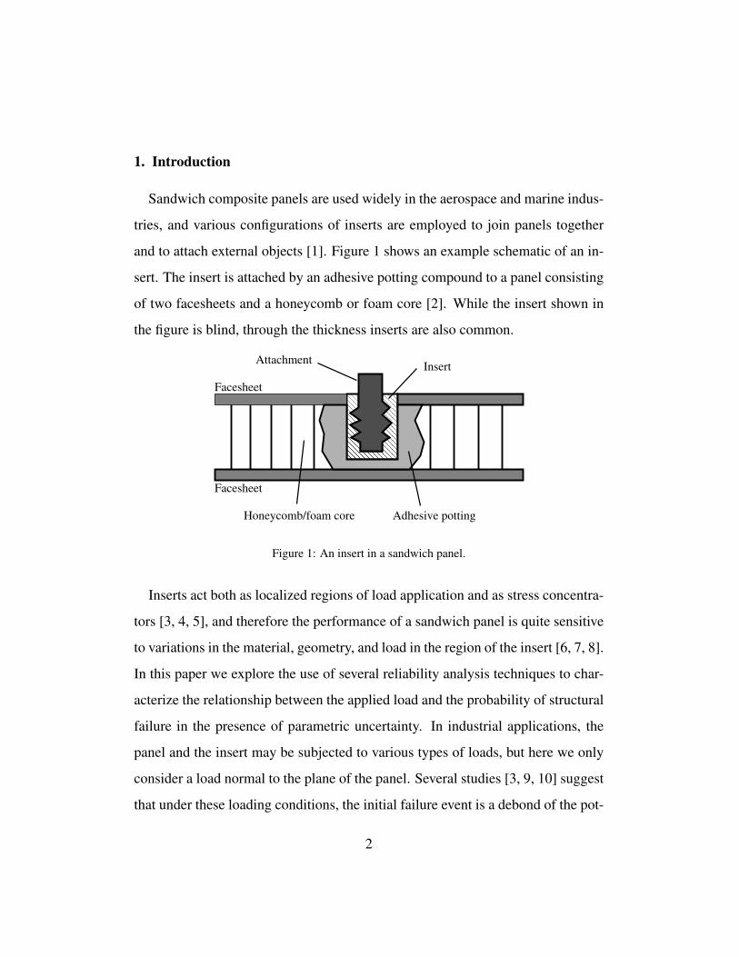
and to attach external objects [1]. Figure 1 shows an example schematic of an in-

sert. The insert is attached by an adhesive potting compound to a panel consisting

of two facesheets and a honeycomb or foam core [2]. While the insert shown in

the figure is blind, through the thickness inserts are also common.

Facesheet

Facesheet

Adhesive potting

InsertAttachment

Honeycomb/foam core

Figure 1: An insert in a sandwich panel.

Inserts act both as localized regions of load application and as stress concentra-

tors [3, 4, 5], and therefore the performance of a sandwich panel is quite sensitive

to variations in the material, geometry, and load in the region of the insert [6, 7, 8].

In this paper we explore the use of several reliability analysis techniques to char-

acterize the relationship between the applied load and the probability of structural

failure in the presence of parametric uncertainty. In industrial applications, the

panel and the insert may be subjected to various types of loads, but here we only

consider a load normal to the plane of the panel. Several studies [3, 9, 10] suggest

that under these loading conditions, the initial failure event is a debond of the pot-

2

ting from the core, followed by buckling of the honeycomb and fracture/yield of

the facesheets. However, we are unaware of any studies addressing reliability of

these structures in the presence of material and geometric variability.

For simplicity and efficiency, we use a one-dimensional axisymmetric model [11]

of a sandwich panel in our study. The structure consists of four components: two

facesheets, a honeycomb core, and the adhesive potting. It is important to note

that though the honeycomb buckles under small loads, the effect of this buck-

ling is not obvious in load-displacement curves from pull-out tests and three-point

bend tests [1, 10]. Thus, a single criterion for localized failure is an insufficient

indicator of macroscopic failure. Since macroscopic failure is of most interest to

design engineers, we consider two multi-component failure criteria. In the first

situation, system failure is assumed to have occurred when any two of the struc-

tural components satisfy certain failure criteria, and in the second situation, failure

occurs when any three components fail.

Sources of uncertainty in the sandwich-insert model include the geometry, the

material properties, and the applied loads. A distinction could possibly be made

between inherent variability (or aleatoric uncertainty) and reducible uncertainty

(or epistemic uncertainty) [12], but for the purpose of this study, all uncertainty

is assumed to be due to inherent variability. In the event of improvement in our

knowledge of the materials or loads, that new knowledge will change only the

expected values and probability distributions that we used to characterize the vari-

ability in our reliability analysis. We ignore detailed micromechanical causes of

variability and focus only on the macroscopically observable statistics. Normal

distributions with assumed standard deviations are used for parameters for which

sufficient data are not available.

3

The simplest method for calculating the probability of failure is Monte Carlo

sampling. However, this method is inefficient for situations with low failure prob-

abilities, so several methods, including the First-order reliability method (FORM) [13],

line sampling [14], and subset simulation [15] have been developed to reduce the

computational cost of determining low probabilities of failure. The principal find-

ing of our work is that for problems with a complex failure sequence and multiple

failure regions within the parameter space, subset simulation is the most efficient

method for determining the structural reliability at low failure probabilities. How-

ever, for failure probabilities of the order typically dealt with by composite de-

signers, none of the advanced reliability analysis methods demonstrate a clear

advantage over Monte Carlo sampling.

The paper is organized as follows. In Section 2, we describe the one-dimensional

axisymmetric model of a sandwich panel with an insert. Comparisons of the

theory with one- and two-dimensional finite element simulations are provided.

Reliability theory and various approaches for uncertainty propagation are briefly

explained in Section 3. In Section 4, finite element simulations are used to de-

termine the estimated reliability of sandwich composites with inserts for various

levels of parameter variability. The results are discussed and conclusions drawn

in Section 5.

2. Modeling sandwich panels with inserts

The numerical simulation of sandwich structures containing inserts can be com-

putationally expensive. This is particularly true when the goal is a statistical anal-

ysis of the effect of variable input parameters on the response of the structure.

Simplified theories of sandwich structures provide an efficient means of reliabil-

4

ity analysis under these circumstances. Models of sandwich structures can be

broadly classified into the following types:

• Single- and multi-layer layer models that do not account for changes in

thickness. Such models include first-order linear models [16], higher-order

linear models [17], and geometrically-exact nonlinear models [18].

• Single- and multi-layer models that do account for thickness changes. These

include linear single-layer models [19, 20, 21], nonlinear single-layer mod-

els [22, 23, 24, 25, 26], and linear multi-layer models [11, 27, 28, 29, 30].

Single-layer models attempt to model the mechanics of sandwich panels in a man-

ner similar to beam and plate theory by adding extra degrees of freedom to a sin-

gle reference surface. Additional effects due to the presence of inserts are difficult

to incorporate into such models. Multi-layer models are more convenient when

modeling inserts in sandwich panels. Also, changes in panel thickness become

important when potted inserts are subjected to pull-out loads. Hence, the linear

theory of sandwich panels with inserts proposed by Thomsen et al. [11, 27, 28]

appears to be appropriate for a reliability analysis of sandwich panels with inserts.

It should be noted that local nonlinear effects (both material and geometric) close

to an insert become pronounced as the deformation proceeds. However, in the

interest of simplicity, we ignore nonlinear effects in this work.

2.1. The Thomsen model

In the original version of the Thomsen model, plate theory was used to develop

three sets of governing equations (for the two facesheets and the core). These

equations were coupled through traction and displacement boundary conditions

at the interfaces between the facesheets and the core. The resulting system of

5

first order ordinary differential equations was solved by Thomsen using a multi-

segment finite-difference method. The insert was assumed to be rigid and the

potting around the insert was modeled as a core material. The model was designed

so that both normal and shear pull-out loads could be applied to the insert.

In our work, we have applied the Thomsen approach to an axisymmetric sand-

wich panel with a through-the-thickness insert. Instead of Thomsen’s numerical

method, we have used a considerably simpler finite element approach to discretize

and solve the governing system of ordinary differential equations.

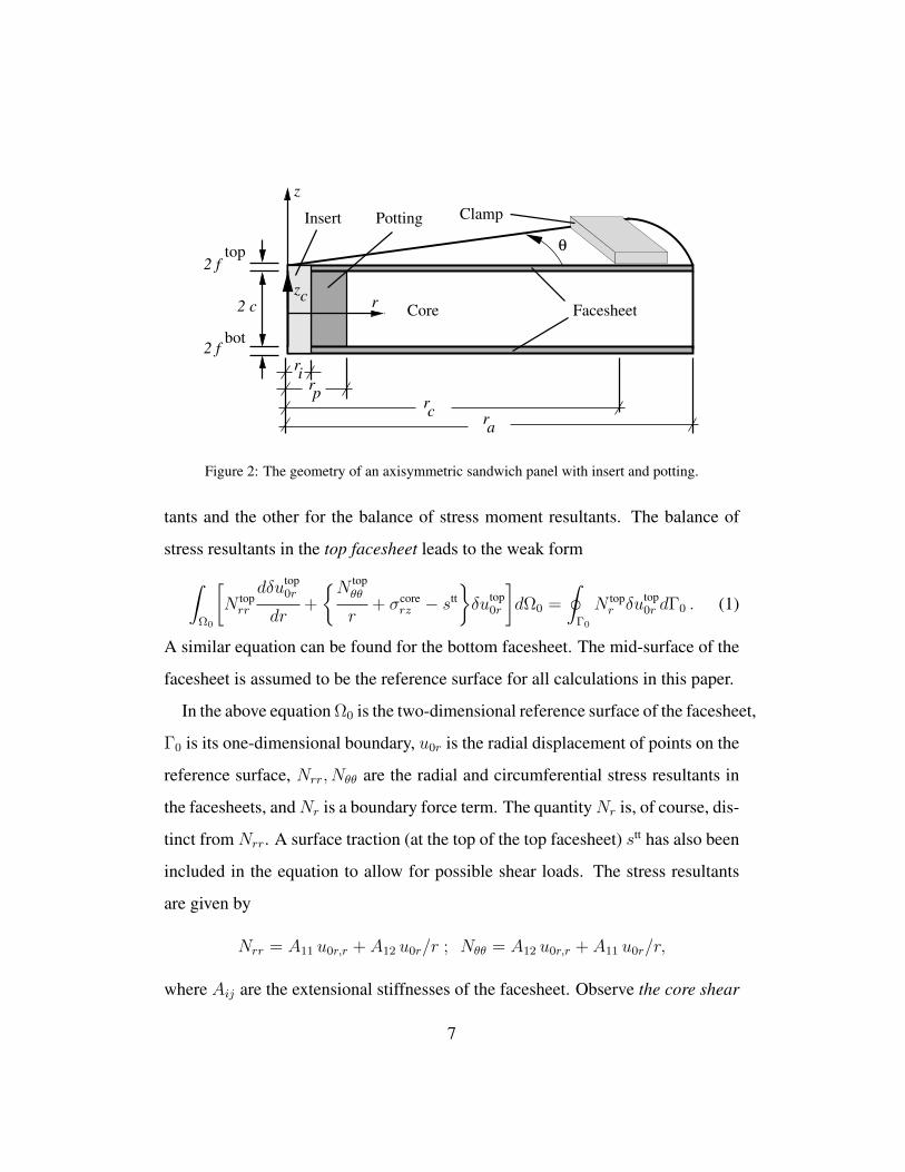
A schematic of an axisymmetric sandwich panel is shown in Figure 2. The

panel has a radius ra and consists of two facesheets and a core. An adhesive

potting of radius rp is used to bond a rigid insert of radius ri to the panel. A vertical

force is applied to the insert in the positive z-direction. A clamp is attached to

the panel at a distance rc from the center to prevent rigid-body motions due to the

applied force. The core thickness is 2c, the top facesheet thickness is 2f top, and the

thickness of the bottom facesheet is 2f bot. The extensional and bending stiffnesses

of the facesheets are Aij = 2fCij and Dij = 2f 3/3Cij , where Cij (i, j = 1, 2)

are components of the stiffness matrix relating the stresses σrr, σθθ to the strains

εrr, εθθ. For the core, the transverse stiffness (C33) is defined by the relation σzz =

C33εzz while the shear compliance (S55) is defined by εrz = S55σrz. The potting

is assumed to have the same behavior as the core, i.e., it is characterized by the

two material constants, C33 and S55.

A detailed derivation of the equations governing the deformation of the panel

(and their weak forms) can be found elsewhere [31]. A summary of the relevant

equations is given below. Conservation of linear and angular momentum in the

facesheets can be expressed as two equations, one for the balance of stress resul-

6

top2 f

bot2 f

ri

rp

ra

rc

2 c

z

θ

Core Facesheetr

Insert Potting Clamp

zc

Figure 2: The geometry of an axisymmetric sandwich panel with insert and potting.

tants and the other for the balance of stress moment resultants. The balance of

stress resultants in the top facesheet leads to the weak form∫Ω0

[N toprr

dδutop0r

dr+

N topθθ

r+ σcore

rz − sttδutop

0r

]dΩ0 =

∮Γ0

N topr δutop

0r dΓ0 . (1)

A similar equation can be found for the bottom facesheet. The mid-surface of the

facesheet is assumed to be the reference surface for all calculations in this paper.

In the above equation Ω0 is the two-dimensional reference surface of the facesheet,

Γ0 is its one-dimensional boundary, u0r is the radial displacement of points on the

reference surface, Nrr, Nθθ are the radial and circumferential stress resultants in

the facesheets, andNr is a boundary force term. The quantityNr is, of course, dis-

tinct from Nrr. A surface traction (at the top of the top facesheet) stt has also been

included in the equation to allow for possible shear loads. The stress resultants

are given by

Nrr = A11 u0r,r + A12 u0r/r ; Nθθ = A12 u0r,r + A11 u0r/r,

where Aij are the extensional stiffnesses of the facesheet. Observe the core shear

7

stress term (σrz) in equation (1. From the point of view of the facesheets, this is

the term that couples the facesheets to the core.

A balance of stress moment resultants in the top facesheet can be expressed as

∫Ω0

[M top

rr

d2δwtop0

dr2+

M topθθ

r− f top (stt − σcore

rz )

dδwtop0

dr

−Ccore

33

2c(wtop

0 − wbot0 )− c

dσcorerz

dr− c

σcorerz

r

δwtop

0

]dΩ0

=

∮Γ0

M topr

dδwtop0

dr−Qtop

z δwtop0

dΓ0. (2)

A similar equation can be found for the bottom facesheet. In the above equation

w0 is the z-direction displacement of the mid-surface of the facesheet and stress

moment resultants are given by:

Mrr = −D11w0,rr −D12w0,r/r ; Mθθ = −D12w0,rr −D11w0,r/r,

where Dij are the bending stiffnesses, Mr is a bending moment, and Qz is a shear

force.

Notice that equation (2) contains another coupling term wbot0 in addition to σcore

rz

which indicates that this equation is couple both to the core and to the bottom

facesheet. Equations (1) and (2) have counterparts when we consider the bot-

tom facesheets and these four coupled equations describe the deformation of the

facesheets. We now need an equation that describes the deformation of the core.

Equilibrium of the core in the presence of the two facesheets requires that the

8

core shear stress satisfies the equation,

∫Ω0

[dσcore

rz

dr

dδσrz

dr+

1

r

(σcorerz

dδσrz

dr+dσcore

rz

drδσrz

)+

( 1

r2+

6Ccore33 Score

55

c2

)σcorerz

−3Ccore

33

2c3

[utop

0r − ubot0r + (f top + c)

dwtop0

dr+(f bot + c

) dwbot0

dr

]δσrz

]dΩ0

=

∮Γ0

(dσcorerz

dr+σcorerz

r

)δσrzdΓ0. (3)

The core shear stress is therefore coupled to the facesheet deformations via the

variables u0r and w0. Therefore we have a system of five coupled equations,

(equations (1) and (2) for both facesheets, and equation (3) for the core), which

can be discretized using finite elements. We have solved these equations with the

finite element code Comsol R©. Quadratic shape functions have been used for the

u-displacement and σ-stress, and cubic Hermite functions for the w-displacement.

2.2. The insert pull-out test

To simulate a pull-out test, a vertical shear traction is applied to the inner surface

of the potting while ur at that location is constrained to zero. The shear stress,

σrz, is set to zero at the free end of the panel, and the points at which the panel is

clamped are constrained such that w0 = 0. Stability of the solution requires that

both the top and the bottom facesheets be clamped. The potting is modelled as

a core with properties that are derived from those of the actual potting material.

Note that the potting, like the core, is assumed to have no extensional stiffness in

the plane of the sandwich panel. There is a discontinuity in material properties

at the potting radius (rp), but no special boundary conditions are required for a

through insert when the appropriate elements are used. For a part-through (or

9

potted) insert, special conditions on the displacements are required (for details

see [31]). However, we only consider through thickness inserts.

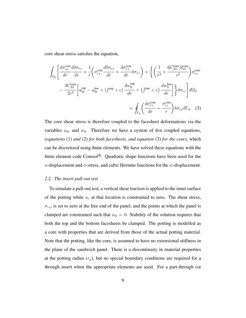
To verify that the one-dimensional model produces reasonable results, it has

been compared with a two-dimensional axisymmetric model simulated with the

Abaqus R© finite element code. Figure 3 shows that the one-dimensional model

provides a reasonable estimate of the core shear stress but underestimates the dis-

placement (compared with the two-dimensional model). The sandwich panel ge-

ometry and material properties for these calculations can be found in [10]. The

stresses in the facesheets are overestimated while those in the potting are underes-

timated by the one-dimensional model and, partly due to the small displacements

and the linear nature of the model, the potting is never observed to fail in our

simulations. However, we ignore these issues in this work and focus on the com-

putation of reliability.

0 10 20 300

0.02

0.04

0.06

0.08

0.1

Distance from insert (mm)

Dis

pla

cem

ent

of

top

of

pan

el (

mm

)

One−dimensional model

Two−dimensional model

0 10 20 30

−3.5

−3

−2.5

−2

−1.5

−1

−0.5

0

Distance from insert (mm)

Sh

ear

stre

ss i

n c

ore

(M

Pa)

Two−dimensional model

One−dimensional model

Figure 3: Comparisons between one-dimensional (solid) and two-dimensional models (dotted).

10

2.3. System failure

The reliability estimates that we seek require the determination of a global fail-

ure surface for the model. There are four components in the structure that can

fail at different loads; the two facesheets, the core, and the potting. One could

take the failure load to be the smallest load at which any of these components fail.

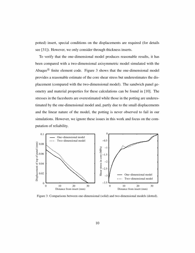
In fact, simulations of detailed honeycomb sandwich panels under pull-out loads

show that the core buckles at relatively small loads (see Figure 4 for an example

of localized buckling at loads less than 1 kN). But load-deflection curves from

the same simulations do not indicate any deviation from linearity at these loads,

let alone failure. Therefore, a global failure surface constructed on the basis of

the “first component to fail” may not be ideal for reliability analyses of sandwich

composites.

0 0.2 0.4 0.6 0.80

1

2

3

4

5

6

Displacement (mm)

Lo

ad (

kN

)

Initial buckling

Figure 4: Localized buckling of the core in an aluminum honeycomb sandwich panel with an

insert under pull-out load.

The procedure that we use to populate the global failure surface is as follows.

A pull-out load is applied to the one-dimensional finite element model. The core

11

and potting stresses (σrz, σzz) and the facesheet stresses (σrr, σθθ) are computed

at each element. The stress in each of these elements is identified and fed into the

failure criterion appropriate for the component to which the element belongs.

In this study, von Mises failure criteria (Tsai-Wu criterion with isotropic prop-

erties) have been used for the aluminum facesheets and the potting. The yield

stresses for these materials have been obtained from [10]. Compressive (buck-

ling) and shear failure stresses in the aluminum honeycomb have been calculated

using the formulae in Gibson and Ashby ([32], p. 171). A quadratic core collapse

criterion that uses the compressive and shear stresses in the core has been used to

flag failure of the honeycomb [33].

The global failure surface is not populated if we observe failure in only one

component. If more than one component appears to have failed, we explore two

options. The first option is designated “two-component failure” and the structure

is assumed to have failed when at least two failure criteria have been exceeded.

The second option is designated “three-component failure”. In this case, the fail-

ure of at least three components is sought before we populate the failure surface.

This approach leads to performance functions that do not necessarily have a high

degree of smoothness and is useful for examining the strengths and weaknesses

of various techniques of reliability analysis.

3. Reliability Analysis

A reliability analysis determines the relationship between the model parame-

ters, θ, a d-dimensional vector with known input probability distributions, and

pf , the probability of structural failure. If g (θ) is a C0 continuous performance

function constructed such that g (θ) ≤ 0 when θ lies in the failure domain and

12

g (θ) > 0 in the safe domain, pf can be defined as:

pf =

∫g(θ)≤0

h (θ) dθ =

∫Rd

1F (θ)h (θ) dθ, (4)

where h(θ) is the joint probability density function of the parameters and 1F (θ) is

an indicator function (equal to one in the failure region and zero elsewhere). For

independent and identically distributed (i.i.d.) parameters, the joint probability

density function can be calculated using

h(θ) =d∏i=1

φ(θi), with φ(θ) =1√2π

e−θ2/2 (5)

where φ is the standard normal probability density function (p.d.f.). Correlated

variables can be converted into an independent set using classical techniques such

as the Nataf transformation. Also, parameters that are not identically distributed

can be usually be transformed and normalized. Therefore, conversion of a non

i.i.d set of parameters into a set that satisfies equation (5) simplifies the analysis

considerably. However, the performance function g(θ) is rarely known explicitly

and typically must be evaluated at individual points in the design space.

The simplest and most reliable method for computing pf is Monte Carlo sam-

pling (MCS) in which N realisations of θ are generated and an estimator, pf =

1N

∑Ni=1 1F (θi), for the failure probability is computed. If the samples are drawn

from the full domain of parameter space, the expression for the coefficient of vari-

ation (CoV) of the Monte Carlo estimator is given by δMC =√

(1− pf )/(pfN).

This expression indicates that in order to achieve a 10% CoV, approximately

100/pf samples must be evaluated. Multiple performance function evaluations

are computationally expensive, so a variety of techniques have been developed to

minimize the required number of simulations.

13

The First Order Reliability Method (FORM) [13] is based on the linearization

of the failure surface at the “design point”, or the most likely point of failure.

Each component of the parameter vector θ is transformed such that θ = T (θ) is

in standard normal space. The performance function is transformed as well, so

that g(θ) = g(T (θ)). The design point is defined as the point θ∗

on the failure

surface that lies closest to the origin. The failure surface is then approximated

as a plane passing through this design point, and the failure probability is given

by pf = Φ(−β) where β = ‖θ∗‖ and Φ is the standard normal cumulative dis-

tribution function (c.d.f.). For many problems, particularly those with relatively

few input parameters and an approximately linear failure surface, FORM is the

most efficient method for calculating the failure probability. But finding the de-

sign point becomes expensive if there are a large number of parameters. Also, it is

not possible to estimate the accuracy of the result without employing an additional

method such as MCS.

Line sampling [14, 34] is a variance reduction technique, meaning it is designed

so that the coefficient of variation (CoV), δLS, of the resulting estimator pf is

smaller than δMC. The key idea behind line sampling is to reduce the dimension

of the problem, and let the failure surface be a function of d − 1 parameters, so

that one parameter, θ1 = g−1 (θ−1), is on the failure surface and the reduced

parameter set is θ−1 = θ2, ..., θd. Like FORM, line sampling requires that θ

be transformed into standard normal space, and the normalized joint probability

density function is given by

h(θ) =d∏i=1

φ(θi) .

The quantity θ1 = g−1(θ−1) is the height of the failure surface at θ−1 in the rotated

14

coordinate system (θ−1, θ1). It can be shown that (see [14]) the probability of

failure is equal to the expectation of the random variable Φ(g−1(θ−1)). A Monte

Carlo estimate of pf is

pf =1

N

N∑i=1

Φ(g−1

(θ

(i)

−1

)). (6)

where Φ is the standard normal cumulative distribution function. Unlike FORM,

it is possible to analytically estimate the accuracy of the pf computed using line

sampling. The variance of the estimator is given by:

Var [pf ] =1

NVar [Φ (g−1)] . (7)

While the CoV of the line sampling estimator, δLS depends on the choice of search

direction θ1, it is always less than or equal to δMC.

Subset simulation [15] is another variance reduction technique, but rather than

dimensional reduction, it employs conditional probability to reduce the variance

of the estimator for pf . Subset simulation is based on the fact that the probability

of a rare failure event can be expressed as the product of the probabilities of more

frequent intermediate events. For example, given a failure event F , let F1 ⊂ F2 ⊂

... ⊂ Fm = F be a decreasing sequence of failure events. Using the definition of

conditional probability, the probability of failure is given by:

pf = P (Fm) = P

(m⋂i=1

Fi

)= P (F1)

m−1∏i=1

P (Fi|Fi−1) . (8)

The key to the implementation of subset simulation is the ability to generate sam-

ples according to the conditional distribution of θ given that it lies in Fi. Markov

chain Monte Carlo simulation is an efficient method for generating samples ac-

cording to an arbitrary distribution, and in this case, a modified Metropolis algo-

rithm is used to generate a Markov chain with the stationary distribution q(·|Fi).

15

This algorithm is described in Appendix A. As with line sampling, the coefficient

of variation of the estimator generated by subset simulation can be calculated di-

rectly, and the details of this calculation can be found in [15].

4. Results

In the previous section we have seen that MCS is expensive if the desired pf is

small. Hundreds, or even thousands, of Monte Carlo simulations may be needed

before we can be confident that a structure will not fail at given load. This is

the primary reason for the lack of penetration of reliability analysis in the routine

design of sandwich composite structures. We have also examined a few methods

that have been developed in recent years with the aim of reducing the number

of simulations needed. Can these advanced techniques be employed to reduce

the number of simulations needed for an accurate analysis of the reliability of

sandwich composites? The results in this section suggest that, in general, the

answer is no.

To evaluate the performance of each technique, the probability of failure of a

sandwich composite with an insert was computed over a range of applied loads,

and calculated failure probabilities, coefficients of variation, and iteration counts

for the four techniques were then compared for each load. Two methods of deter-

mining global failure were examined, two-component failure and three-component

failure, as discussed in Section 2.3.

4.1. Input statistics and sensitivity

The sandwich panel geometry and material properties were obtained from [10].

The input parameter vector, θ, consisted of 19 parameters describing the geom-

etry, stiffnesses, and failure stresses. The geometric parameters were ra, rc, rp,

16

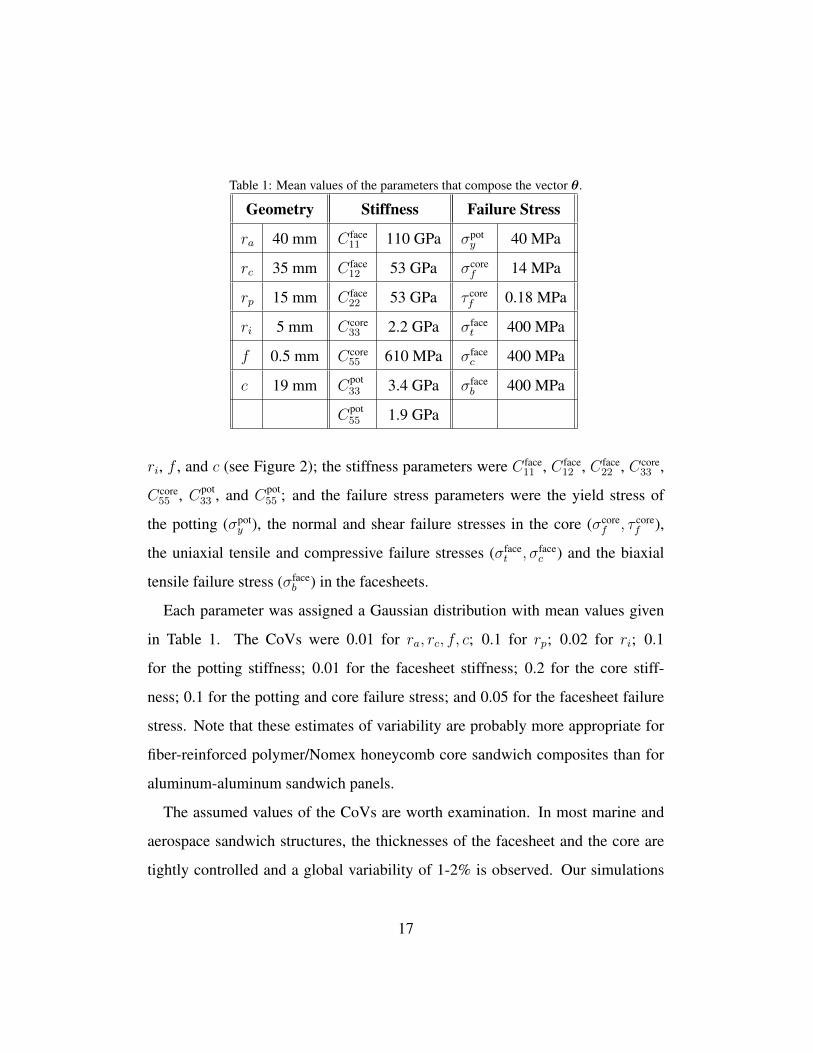
Table 1: Mean values of the parameters that compose the vector θ.

Geometry Stiffness Failure Stress

ra 40 mm C face11 110 GPa σpot

y 40 MPa

rc 35 mm C face12 53 GPa σcore

f 14 MPa

rp 15 mm C face22 53 GPa τ core

f 0.18 MPa

ri 5 mm Ccore33 2.2 GPa σface

t 400 MPa

f 0.5 mm Ccore55 610 MPa σface

c 400 MPa

c 19 mm Cpot33 3.4 GPa σface

b 400 MPa

Cpot55 1.9 GPa

ri, f , and c (see Figure 2); the stiffness parameters were C face11 , C face

12 , C face22 , Ccore

33 ,

Ccore55 , Cpot

33 , and Cpot55 ; and the failure stress parameters were the yield stress of

the potting (σpoty ), the normal and shear failure stresses in the core (σcore

f , τ coref ),

the uniaxial tensile and compressive failure stresses (σfacet , σface

c ) and the biaxial

tensile failure stress (σfaceb ) in the facesheets.

Each parameter was assigned a Gaussian distribution with mean values given

in Table 1. The CoVs were 0.01 for ra, rc, f, c; 0.1 for rp; 0.02 for ri; 0.1

for the potting stiffness; 0.01 for the facesheet stiffness; 0.2 for the core stiff-

ness; 0.1 for the potting and core failure stress; and 0.05 for the facesheet failure

stress. Note that these estimates of variability are probably more appropriate for

fiber-reinforced polymer/Nomex honeycomb core sandwich composites than for

aluminum-aluminum sandwich panels.

The assumed values of the CoVs are worth examination. In most marine and

aerospace sandwich structures, the thicknesses of the facesheet and the core are

tightly controlled and a global variability of 1-2% is observed. Our simulations

17

model a standard insert pull-out test for which the radius of the panel and the

radius of the clamped region are also tightly specified. There is less control over

the radius of the insert, but the variability can still be assumed to be quite small.

However, the effective radius of the adhesive potting can change dramatically

depending on the location of the insert relative to the honeycomb geometry; a

10-20% difference between two samples is quite routine. The facesheet stiffness

varies little between samples, especially if the facesheet is thin. On the other hand,

we have found that the core stiffness can be significantly different from sample to

sample because it depends strongly on the geometry of the honeycomb. This is

even more so when we consider foam cores. The stiffness of the potting is affected

by the presence of voids. The 10% variability that we have assumed attempts to

take the effect of gas pockets into account. The variability in the failure stress of

the potting does not take voids into consideration and hence is lower than that for

the potting stiffness. The core failure stress is dominated by localized buckling

and tensile failure and the variation is less than that of the core stiffness, which is

a global quantity. The variation in the facesheet failure stress is usually quite small

for thin facesheets. However, larger CoVs should be used for thick facesheets.

It is implicit in the above that the parameters are independent. However, there is

a correlation between the geometry of the honeycomb and its stiffness and strength

properties. Simplified models, such as those discussed in [32], can be used to

reduce the number of independent variables. The resulting expressions, though

exact, can be quite involved. If enough experimental data is available on the dis-

tributions of the parameters, correlations may be computed and the vector θ can

be transformed into an independent set using classical transformations.

A sensitivity analysis can also be used to reduce the length of the vector θ. We

18

rp

ri

σface

t

σfacec

σface

b

C55

core

0.1

0.2

0.3

0.4

c

σface

b

Ccore

55

σface

t

σface

c

C33

core

ri rp0.1

0.2

0.3

0.4

f

c

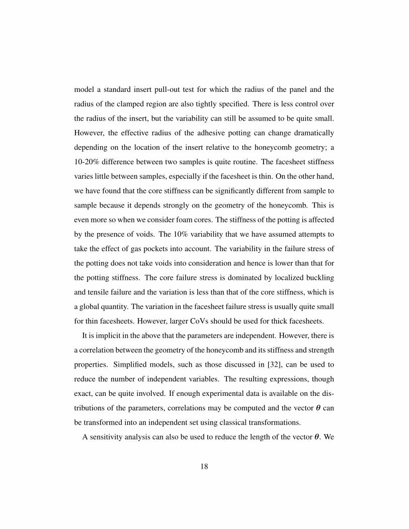
Figure 5: Rosette plots showing the sensitivity of global failure to the input parameters at a load

where the probability of failure is ∼50%. The plot on left is for two-component failure and that

on the right is for three-component failure. Only parameters with a sensitivity index greater than

0.01 are labelled.

have not used sensitivity information for the reliability calculations in this work.

However, for completeness, we have calculated, using Sobol’s Method [35], the

total global sensitivity indices for each of the input variables. In order to best

identify the factors that determine structural failure, these analyses were carried

out at loads where the probability of failure is near 50%: 3.25 kN for the two-

component failure model and 3.55 kN for the three-component failure model. The

rosette plots in Figure 5 indicate which of the input parameters have the largest

impact for the two- and three-component cases. Our calculations with the Thom-

sen model suggest that the critical mode in both cases is the failure of one or

both facesheets and it is not surprising that the most critical parameters are the

facesheet failure strengths. The parameters that govern the shear stiffness of the

core, Ccore55 and c play a large role as well, as these determine how much of the

pullout load must be carried by the facesheets.

19

2.5 3 3.5 40

0.2

0.4

0.6

0.8

1

Monte Carlo

FORM

Line Sampling

Subset Simulation

Load (kN)

Fai

lure

pro

bab

ilit

y

2.5 3 3.5 410

−4

10−3

10−2

10−1

100

Monte Carlo

FORM

Line Sampling

Subset Simulation

Load (kN)

Fai

lure

pro

bab

ilit

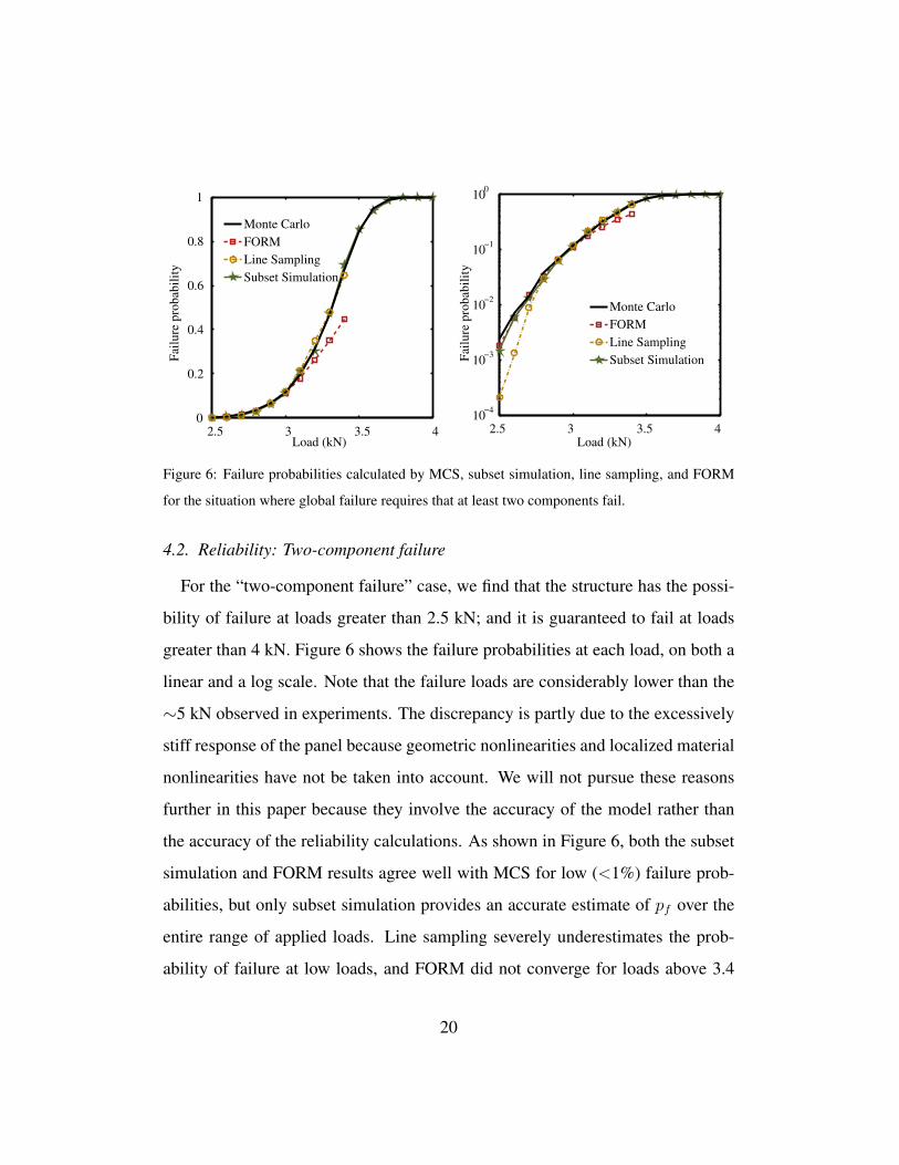
yFigure 6: Failure probabilities calculated by MCS, subset simulation, line sampling, and FORM

for the situation where global failure requires that at least two components fail.

4.2. Reliability: Two-component failure

For the “two-component failure” case, we find that the structure has the possi-

bility of failure at loads greater than 2.5 kN; and it is guaranteed to fail at loads

greater than 4 kN. Figure 6 shows the failure probabilities at each load, on both a

linear and a log scale. Note that the failure loads are considerably lower than the

∼5 kN observed in experiments. The discrepancy is partly due to the excessively

stiff response of the panel because geometric nonlinearities and localized material

nonlinearities have not be taken into account. We will not pursue these reasons

further in this paper because they involve the accuracy of the model rather than

the accuracy of the reliability calculations. As shown in Figure 6, both the subset

simulation and FORM results agree well with MCS for low (<1%) failure prob-

abilities, but only subset simulation provides an accurate estimate of pf over the

entire range of applied loads. Line sampling severely underestimates the prob-

ability of failure at low loads, and FORM did not converge for loads above 3.4

20

2.5 3 3.5 40

0.5

1

1.5

2

2.5

Monte Carlo

Subset Simulation

Load (kN)

Nu

mb

er

of

itera

tio

ns

(x 1

0,0

00

)

2.5 3 3.5 40

0.05

0.1

0.15

0.2

0.3

0.25

Load (kN)

Co

eff

icie

nt

of

vari

ati

on

Monte Carlo

Subset Simulation

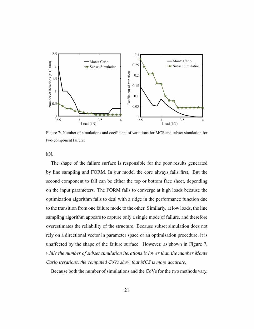
Figure 7: Number of simulations and coefficient of variations for MCS and subset simulation for

two-component failure.

kN.

The shape of the failure surface is responsible for the poor results generated

by line sampling and FORM. In our model the core always fails first. But the

second component to fail can be either the top or bottom face sheet, depending

on the input parameters. The FORM fails to converge at high loads because the

optimization algorithm fails to deal with a ridge in the performance function due

to the transition from one failure mode to the other. Similarly, at low loads, the line

sampling algorithm appears to capture only a single mode of failure, and therefore

overestimates the reliability of the structure. Because subset simulation does not

rely on a directional vector in parameter space or an optimisation procedure, it is

unaffected by the shape of the failure surface. However, as shown in Figure 7,

while the number of subset simulation iterations is lower than the number Monte

Carlo iterations, the computed CoVs show that MCS is more accurate.

Because both the number of simulations and the CoVs for the two methods vary,

21

2

4

6

8

10

0

10−3

10−2

10−1

100

Monte Carlo (Theory)

Subset Simulation

Nu

mb

er o

f it

erat

ion

s (x

10

00

)

Probability of failure

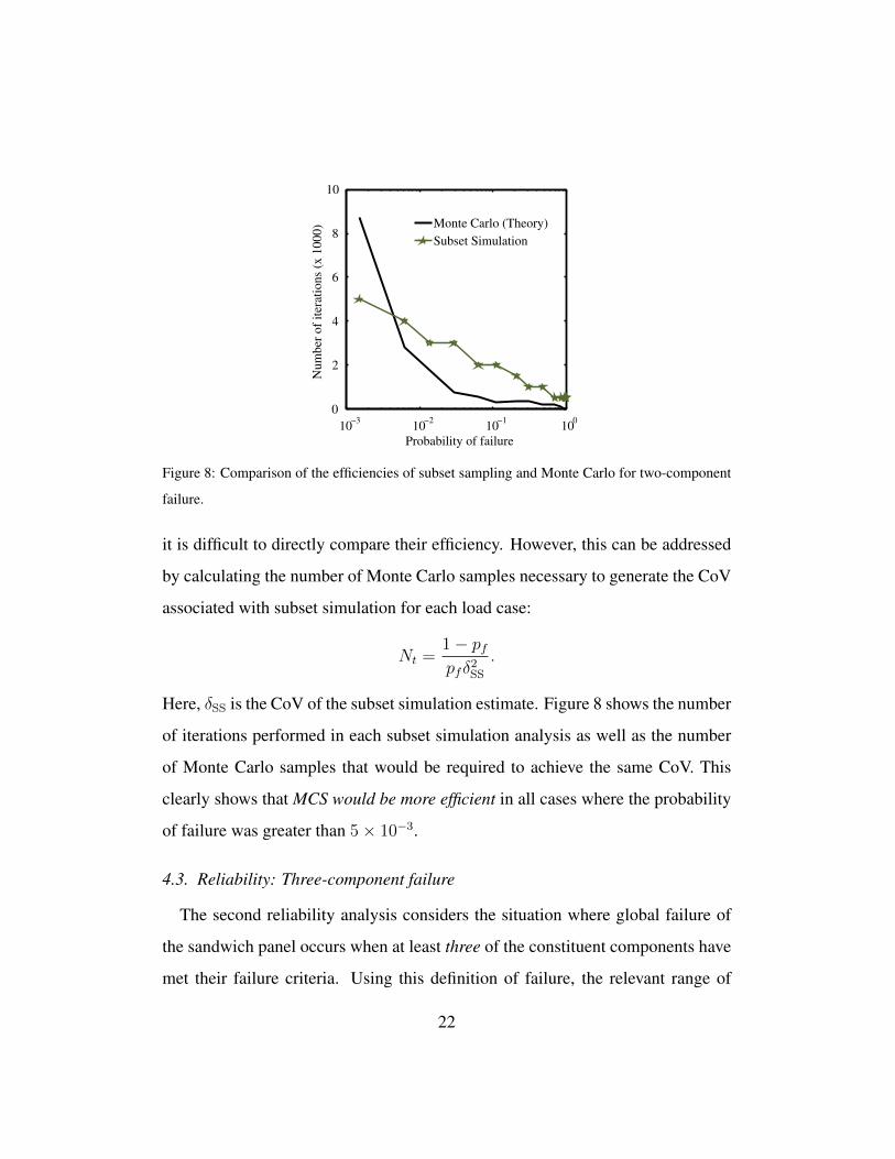
Figure 8: Comparison of the efficiencies of subset sampling and Monte Carlo for two-component

failure.

it is difficult to directly compare their efficiency. However, this can be addressed

by calculating the number of Monte Carlo samples necessary to generate the CoV

associated with subset simulation for each load case:

Nt =1− pfpfδ2

SS

.

Here, δSS is the CoV of the subset simulation estimate. Figure 8 shows the number

of iterations performed in each subset simulation analysis as well as the number

of Monte Carlo samples that would be required to achieve the same CoV. This

clearly shows that MCS would be more efficient in all cases where the probability

of failure was greater than 5× 10−3.

4.3. Reliability: Three-component failure

The second reliability analysis considers the situation where global failure of

the sandwich panel occurs when at least three of the constituent components have

met their failure criteria. Using this definition of failure, the relevant range of

22

2.8 3.2 3.6 4 4.40

0.2

0.4

0.6

0.8

1

Load (kN)

Fai

lure

pro

bab

ilit

y

Monte Carlo

Line Sampling

Subset Simulation

10−4

10−3

10−2

10−1

100

2.8 3.2 3.6 4 4.4

Monte Carlo

Line Sampling

Subset Simulation

Load (kN)

Fai

lure

pro

bab

ilit

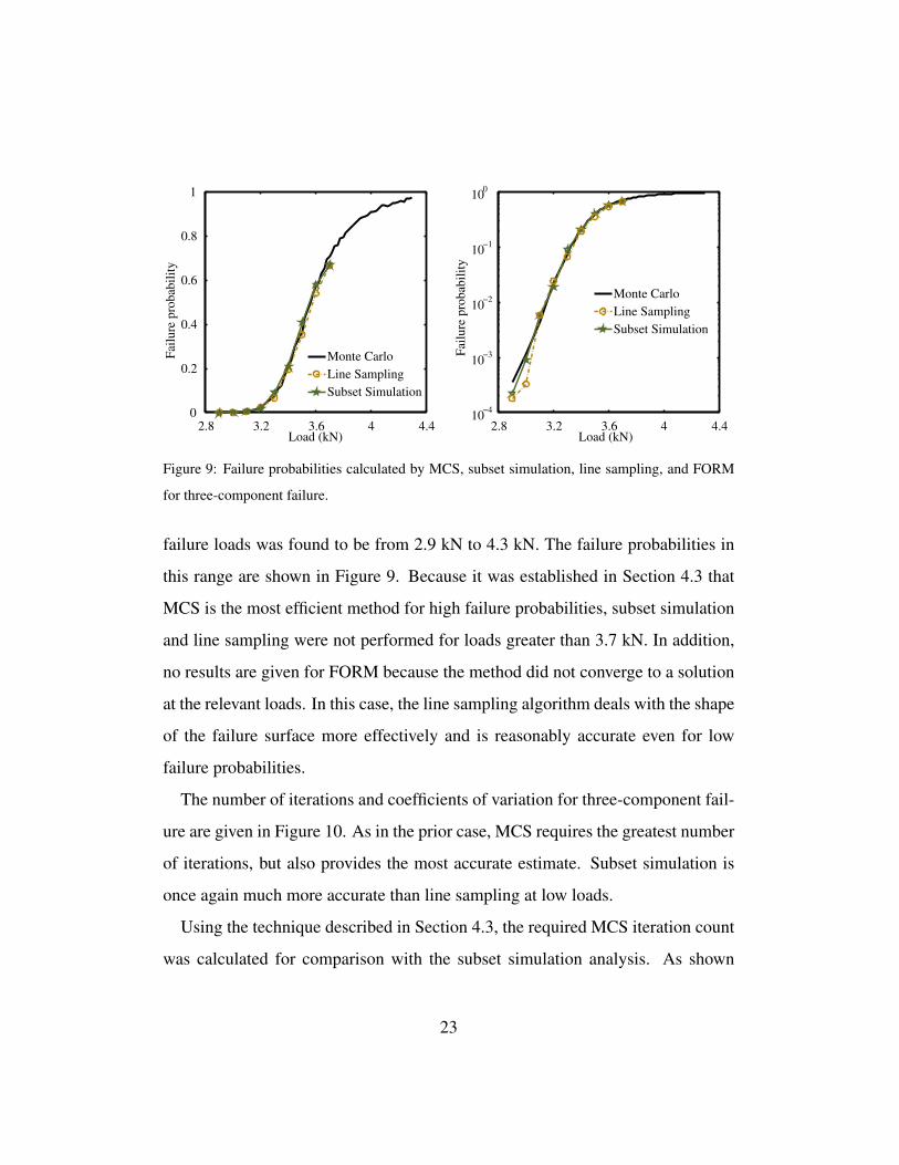
yFigure 9: Failure probabilities calculated by MCS, subset simulation, line sampling, and FORM

for three-component failure.

failure loads was found to be from 2.9 kN to 4.3 kN. The failure probabilities in

this range are shown in Figure 9. Because it was established in Section 4.3 that

MCS is the most efficient method for high failure probabilities, subset simulation

and line sampling were not performed for loads greater than 3.7 kN. In addition,

no results are given for FORM because the method did not converge to a solution

at the relevant loads. In this case, the line sampling algorithm deals with the shape

of the failure surface more effectively and is reasonably accurate even for low

failure probabilities.

The number of iterations and coefficients of variation for three-component fail-

ure are given in Figure 10. As in the prior case, MCS requires the greatest number

of iterations, but also provides the most accurate estimate. Subset simulation is

once again much more accurate than line sampling at low loads.

Using the technique described in Section 4.3, the required MCS iteration count

was calculated for comparison with the subset simulation analysis. As shown

23

2.8 3.2 3.6 4 4.40

0.5

1

1.5

2

2.5

Load (kN)

Nu

mb

er o

f it

erat

ion

s (x

10

,00

0)

Monte Carlo

Line Sampling

Subset Simulation

2.8 3.2 3.6 4 4.40

0.2

0.4

0.6

0.8

0.9

Load (kN)

Co

effi

cien

t o

f v

aria

tio

n

Monte Carlo

Line Sampling

Subset Simulation

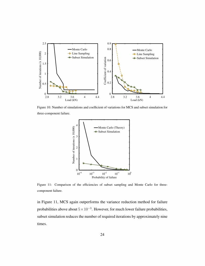
Figure 10: Number of simulations and coefficient of variations for MCS and subset simulation for

three-component failure.

10−4

10−3

10−2

10−1

100

0

1

2

3

4

Probability of failure

Nu

mb

er o

f it

erat

ion

s (x

10

,00

0)

Monte Carlo (Theory)

Subset Simulation

Figure 11: Comparison of the efficiencies of subset sampling and Monte Carlo for three-

component failure.

in Figure 11, MCS again outperforms the variance reduction method for failure

probabilities above about 5×10−3. However, for much lower failure probabilities,

subset simulation reduces the number of required iterations by approximately nine

times.

24

−15

−10

−5

0

5

0.9 1 1.2 1.4

Monte Carlo

Weibull

Gumbel

log(Load −kN) − Two failure criteria met

log

[−lo

g(1

−p

)]f

2.8 3.2 3.6 4 4.4−5

0

5

10

Monte Carlo

Weibull

Gumbel

Load (kN) − Three failure criteria met

)]f

−lo

g[−

log

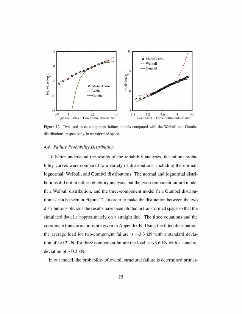
(pFigure 12: Two- and three-component failure models compared with the Weibull and Gumbel

distributions, respectively, in transformed space.

4.4. Failure Probability Distribution

To better understand the results of the reliability analyses, the failure proba-

bility curves were compared to a variety of distributions, including the normal,

lognormal, Weibull, and Gumbel distributions. The normal and lognormal distri-

butions did not fit either reliability analysis, but the two-component failure model

fit a Weibull distribution, and the three-component model fit a Gumbel distribu-

tion as can be seen in Figure 12. In order to make the distinction between the two

distributions obvious the results have been plotted in transformed space so that the

simulated data lie approximately on a straight line. The fitted equations and the

coordinate transformations are given in Appendix B. Using the fitted distribution,

the average load for two-component failure is ∼3.3 kN with a standard devia-

tion of ∼0.2 kN; for three component failure the load is ∼3.6 kN with a standard

deviation of ∼0.3 kN.

In our model, the probability of overall structural failure is determined primar-

25

ily by facesheet failure, due to the fact that the core and the potting fail at very

low and very high loads, respectively. Therefore, in the two component case,

structural failure occurs when at least one facesheet fails (the minimum of the two

criteria), and in the three component case, failure occurs when both facesheets fail

(the maximum). Because a stress based reliability analysis captures the maximum

values of the failure criteria within each component, the distribution of failure

loads is typically described by an extreme value distribution. The Weibull distri-

bution describes the distribution of the minimum of a set of extreme values, and

the Gumbel distribution describes the maximum of a set of extreme values, so the

results given above are reasonable.

5. Discussion and Conclusions

This study has shown that in certain circumstances, variance reduction meth-

ods may be useful for reducing the amount of computational effort required for

the reliability analysis of a composite sandwich structure. When the probability of

failure is anticipated to be below about 0.1%, subset simulation provides a signif-

icant reduction in the number of required structural evaluations while maintaining

the flexibility associated with MCS. Line sampling and FORM are not as effective

for problems in composites due to the fact that they do not deal effectively with

multiple failure modes. There are some special situations, particularly for non-

critical inserts in marine composites, where relatively large failure probabilities

in the range of 0.5% to 5% are acceptable. This study has shown that none of

the available reliability analysis techniques can improve upon MCS in this range.

For lower failure probabilities, though subset simulation provides a stable and

more efficient alternative, the required number of simulations continues to be in

26

the thousands. The implication of this result is that accurate characterisation of

the reliability of composite structures will require either parallel computers capa-

ble of carrying out thousands of detailed simulations in a short period of time or

the development of reduced-order models that capture the important facets of the

behavior of the structure.

Acknowledgment

This work has been supported by The Foundation for Research Science and

Technology of New Zealand through Grant UOAX0710 and Altitude Aerospace

Interiors. We would also like to thank Dr. Emilio Calius, Dr. Mark Battley, and

Dr. Temoana Southward for introducing us to the problem. Thanks are also due

to an anonymous reviewer for pointing out inconsistencies and helping improve

the paper.

Glossary

pf probability of failure

CoV coefficient of variation

ri radius of insert

rp radius of potting

rc radius of clamped region

ra radius of panel

2c core thickness

2f facesheet thickness

Cij elastic stiffness of facesheet

C33 elastic transverse stiffness of core/potting

27

C33 elastic shear stiffness of core/potting

S55 elastic shear compliance of core/potting

Aij extensional stiffness of facesheet

Dij bending stiffness of facesheet

σrr radial stress

σθθ circumferential stress

σrz transverse shear stress

σzz transverse normal stress

εrr radial strain

εθθ circumferential strain

εrz transverse shear strain

Ω0 reference surface of facesheet

Γ0 boundary of reference surface

Nrr radial stress resultant

Nθθ circumferential stress resultant

u0r radial displacement

s external shear traction

Nr external normal force on Γ0

Mr external moment on Γ0

Qz external shear force on Γ0

Mrr radial stress moment resultant

Mθθ circumferential stress moment resultant

w0 out-of-plane displacement

θ vector of uncertain parameters

θ normalized vector of uncertain parameters

28

g(θ) performance function

h(θ) joint probability density function

F failure event

σy yield stress

σf normal stress at failure

τf shear stress at failure

σt uniaxial tensile stress at failure

σc uniaxial compressive stress at failure

σc biaxial tensile stress at failure

Φ standard normal cumulative distribution function

φ standard normal probability density function

References

[1] S. Heimbs, M. Pein, Failure behaviour of honeycomb sandwich corner joints

and inserts, Composite Structures 89 (4) (2009) 575–588.

[2] N. Raghu, M. Battley, T. Southward, Strength variability of inserts in sand-

wich panels, in: Proc. , Eighth International Conference on Sandwich Struc-

tures, Porto, 2008, pp. 558–569.

[3] P. Bunyawanichakul, B. Castanie, J.-J. Barrau, Experimental and numerical

analysis of inserts in sandwich structures, Applied Composite Materials 12

(2005) 177–191.

29

[4] M. A. Roth, Development of new reinforced load introductions for sand-

wich structures, in: O. T. Thomsen, E. Bozhevolnaya, A. Lyckegaard (Eds.),

Sandwich Structures 7: Advancing with Sandwich Structures and Materials,

Spirnger, Dordrecht, 2005, pp. 987–996.

[5] E. V. Iarve, R. Kim, D. Mollenhauer, Three-dimensional stress analysis and

Weibull statistics based strength prediction in open hole composites, Com-

posites Part A: Applied Science and Manufacturing 38 (1) (2007) 174–185.

[6] E. V. Iarve, D. Mollenhauer, T. J. Whitney, R. Kim, Strength prediction in

composites with stress concentrations: Classical Weibull and critical failure

volume methods with micromechanical considerations, Journal of Materials

Science 41 (20) (2006) 6610–6621.

[7] S. Sihn, E. V. Iarve, A. K. Roy, Asymptotic analysis of laminated composites

with countersunk open- and fastened-holes, Composites Science and Tech-

nology 66 (14) (2006) 2479–2490.

[8] K.-I. Song, J.-Y. Choi, J.-H. Kweon, J.-H. Choi, K.-S. Kim, An experimental

study of the insert joint strength of composite sandwich structures, Compos-

ite Structures 86 (2008) 107–113.

[9] N. Raghu, M. Battley, T. Southward, Strength variability of inserts in sand-

wich panels, Journal of Sandwich Structures and Materials 11 (6) (2009)

501.

[10] G. Bianchi, G. S. Aglietti, G. Richardson, Static Performance of Hot Bonded

and Cold Bonded Inserts in Honeycomb Panels, Journal of Sandwich Struc-

tures and Materials (2010) doi:10.1177/1099636209359840.

30

[11] O. T. Thomsen, W. Rits, Analysis and design of sandwich plates with inserts

- a higher order sandwich plate theory, Composites Part B 29B (1998) 795–

807.

[12] J. C. Helton, J. D. Johnson, W. L. Oberkampf, Verification of the calculation

of probability of loss of assured safety in temperature-dependent systems

with multiple weak and strong links, Reliability Engineering and System

Safety 92 (10) (2007) 1363–1373.

[13] A. M. Hasofer, N. C. Lind, Exact and invariant second-moment code format,

ASCE J. Eng. Mech. 100 (EM 1) (1974) 111–121.

[14] P. S. Koutsourelakis, H. J. Pradlwarter, G. I. Schueller, Reliability of struc-

tures in high dimensions, Part I: Algorithms and applications, Probabilistic

Engineering Mechanics 19 (4) (2004) 409–417.

[15] S. K. Au, J. L. Beck, Estimation of small failure probabilities in high di-

mensions by subset simulation, Probabilistic Engineering Mechanics 16 (4)

(2001) 263–277.

[16] F. J. Plantema, Sandwich Construction, John Wiley and Sons, New York,

1966.

[17] W. S. Burton, A. K. Noor, Assessment of continuum models for sandwich

panel honeycomb cores, Comput. Methods Apl. Mech. Engrg. 145 (1997)

341–360.

[18] L. Vu-Quoc, I. K. Ebcioglu, H. Deng, Dynamic formulation for

geometrically-exact sandwich shells, Int. J. Solids Struct. 34 (20) (1997)

2517–2548.

31

[19] T. Anderson, E. Madenci, W. S. Burton, J. Fish, Analytical solution of finite-

geometry composite panels under transient surface loading, Int. J. Solids

Struct. 35 (12) (1998) 1219–1239.

[20] A. Barut, E. Madenci, J. Heinrich, A. Tessler, Analysis of thick sandwich

construction by a 3,2-order theory, Int. J. Solids Struct. 38 (2001) 6063–

6077.

[21] A. Barut, E. Madenci, T. Anderson, A. Tessler, Equivalent single-layer the-

ory for a complete stress field in sandwich panels under arbitrary distributed

loading, Composite Structures 58 (2002) 483–495.

[22] L. Vu-Quoc, I. K. Ebcioglu, General multilayer geometrically-exact

beams/1-d plates with deformable layer thickness: Equations of motion, Z.

Angew. Math. Mech. 80 (2000) 113–136.

[23] Y. Frostig, O. T. Thomsen, I. Sheinman, On the non-linear high-order theory

of unidirectional sandwich panels with a transversely flexible core, Int. J.

Solids Struct. 42 (2005) 1443–1463.

[24] R. A. Arciniega, J. N. Reddy, Large deformation analysis of functionally

graded shells, Int. J. Solids Struct. 44 (2007) 2036–2052.

[25] R. A. Arciniega, J. N. Reddy, Tensor-based finite element formulation for

geometrically nonlinear analysis of shell structures, Comput. Methods Appl.

Mech. Engrg. 196 (2007) 1048–1073.

[26] J. Hohe, L. Librescu, Recent results on the effect of the transverse core com-

pressibility on the static and dynamic response of sandwich structures, Com-

posites: Part B 39 (2008) 108–119.

32

[27] O. T. Thomsen, Sandwich plates with ’through-the-thickness’ and ’fully pot-

ted’ inserts: evaluation of differences in structural performance, Composites

Structures 40 (2) (1998) 159–174.

[28] O. T. Thomsen, High-order theory for the analysis of multi-layer plate as-

semblies and its application for the analysis of sandwich panels with termi-

nating plies, Composites Structures 50 (2000) 227–238.

[29] O. Rabinovitch, Y. Frostig, High-order behavior of fully bonded and delam-

inated circular sandwich plates with laminated face sheets and a “soft” core,

Int. J. Solids Struct. 39 (2002) 3057–3077.

[30] G. M. Kulikov, E. Carrera, Finite deformation higher-order shell models and

rigid-body motions, Int. J. Solids Struct. 45 (2008) 3153–3172.

[31] B. Banerjee, B. Smith, The Thomsen model of inserts in sandwich compos-

ites: An evaluation, arXiv:cond-mat 1009.5431v1 (2010) 1–30.

[32] L. Gibson, M. Ashby, Cellular solids: structure and properties, Cambridge

Univ Pr, 1999.

[33] D. Mohr, M. Doyoyo, Deformation-induced folding systems in thin-walled

monolithic hexagonal metallic honeycomb, International journal of solids

and structures 41 (11-12) (2004) 3353–3377.

[34] G. I. Schueller, H. J. Pradlwarter, P. S. Koutsourelakis, A critical appraisal

of reliability estimation procedures for high dimensions, Probabilistic Engi-

neering Mechanics 19 (4) (2004) 463–474.

33

[35] I. Sobol’, Sensitivity estimates for nonlinear mathematical models, MMCE

1 (4) (1993) 407–414.

Appendix A. Subset simulation implementation details

Appendix A.1. Markov Chain Monte Carlo

The key to the implementation of subset simulation is the ability to generate

samples according to the conditional distribution of θ given that it lies in Fi:

q(θ|Fi) = q(θ)1Fi(θ)/P (Fi). Markov-chain Monte Carlo simulation is an ef-

ficient method for generating samples according to an arbitrary distribution. In

our work, a modified Metropolis algorithm is used to generate a Markov chain

with the stationary distribution q(·|Fi). The modified Metropolis algorithm is

a two step process for generating additional samples, and relies on a “proposal

PDF”, p∗j(ξj|θj) for generating samples around each component of θ. The pro-

posal PDF is a one dimensional PDF centered at θj with the symmetry property

p∗j(ξj|θj) = p∗j(θj|ξj). In this study, p∗j is chosen as the uniform distribution with

a width of one standard deviation.

Appendix A.2. Intermediate Failure Events

The second key implementation detail is the choice of the intermediate failure

events F1, ..., Fm−1. While it is possible to choose the conditional failure values

gi a priori, the implementation of the method is more straightforward if the gi

are chosen adaptively so that the conditional probabilities are equal to a fixed

value p0. This is accomplished by choosing gi as the (1 − p0)N th largest value

from g(θ(k)i ) : k = 1, ..., N . The conditional probability p0 is chosen to reflect

a balance between the number of required conditional levels and the number of

34

samples per level. Here, a value of 0.2 has been chosen for low loads, and 0.5 has

been used at higher loads.

Appendix B. Weibull and Gumbel distributions and transformations

The distributions fitted to the results of the Monte Carlo simulations of the two-

and three-component failure models (see Figure 12) were:

pf (x) ≈ 1− e−(x/λ)k = 1− e−(x/3380)18 Two-component failure,

pf (x) ≈ e−e−(x−µ)/β

= e−e−(x−3490)/209

Three-component failure.

The Weibull distribution is defined by the cumulative distribution function:

pw (x) = 1− e−(x/λ)k .

Let the transformation Tw be defined as Tw(f) = log[− log(1 − f)], and let x =

log x. Applying Tw to pw (x) gives:

Tw [pw (x]) = log[− log

(e−(exp x/λ)k

)]= kx− k log λ,

so a plot of x = log x versus Tw (pw) is a straight line. Similarly, the Gumbel

distribution is defined by the c.d.f:

pg(x) = e−e−x−µ

β.

Applying the transformation Tg(f) = − log(− log f) to pg gives:

Tg [pg (x)] = − log[− log

(ee

−(x−µ)/β)]

=1

βx− µ

β,

so x versus Tg (pg (x)) is a line. The transformations Tw and Tg were used to

create the plots shown in Figure 12.

35