RELATIVE GOODS’ PRICES AND PURE INFLATION

November 2007

Ricardo Reis and Mark W. Watson*

Woodrow Wilson School and Department of Economics, Princeton University and the National Bureau of Economic Research

ABSTRACT

This paper uses a dynamic factor model for the quarterly changes in consumption goods’ prices to separate them into three components: idiosyncratic relative-price changes, aggregate relative-price changes, and changes in the unit of account. The model identifies a measure of “pure” inflation: the common component in goods’ inflation rates that has an equiproportional effect on all prices and is uncorrelated with relative price changes at all dates. The estimates of pure inflation and of the aggregate relative-price components allow us to re-examine three classic macro-correlations. First, we find that pure inflation accounts for 15-20% of the variability in overall inflation, so that most changes in inflation are associated with changes in goods’ relative prices. Second, we find that the Phillips correlation between inflation and measures of real activity essentially disappears once we control for goods’ relative-price changes. Third, we find that, at business-cycle frequencies, the correlation between inflation and money is close to zero, while the correlation with nominal interest rates is around 0.5, confirming previous findings on the link between monetary policy and inflation. JEL codes: E31, C43, C32 Keywords: Inflation, Relative prices, Dynamic Factor Models, Phillips relation.

*This paper supersedes and significantly elaborates on some parts of our unpublished working paper, Reis and Watson (2007). We are grateful to several colleagues for their valuable input to this research project. For their support and hospitality, Reis thanks the Hoover Institution at Stanford University under a Campbell national fellowship, Columbia University, and the University of Chicago. The National Science Foundation provided support through grant SES-0617811. The data and replication files for this research are at http://www.princeton.edu/~rreis or at http://www.princeton.edu/~mwatson. Contact: rreis@princeton.edu or mwatson@princeton.edu.

1

1. Introduction

One of the goals of macroeconomics is to explain the aggregate sources of

changes in goods’ prices. If there was a single consumption good in the world, as is often

assumed in models, describing the price changes of consumption would be a trivial

matter. But, in reality, there are many goods and prices, and there is an important

distinction between price changes that are equiproportional across all goods (absolute-

price changes) and changes in the cost of some goods relative to others (relative-price

changes). The goal of this paper is to empirically separate these two sources of price

changes, and to investigate how they affect the key macroeconomic relations involving

inflation.

Our data are the quarterly price changes in each of 187 sectors in the U.S.

personal consumption expenditures (PCE) category of the national income and product

accounts from 1959:1 to 2006:2. Denoting the rate of price change for the i’th good

between dates t-1 and t by πit, and letting πt be the Nx1 vector that collects these goods’

prices, we model their co-movement using a linear factor model:

πt = ΛFt + ut (1)

The k factors in the kx1 vector Ft capture common sources of variation in prices. These

might be due to aggregate shocks affecting all sectors, like changes in aggregate

productivity, government spending, or monetary policy, or they may be due to shocks

that affect many but not all sectors, like changes in energy prices, weather events in

agriculture, or exchange rate fluctuations and the price of tradables. The N×k matrix Λ

contains coefficients (or factor loadings) that determine how each individual good’s price

responds to these shocks. The remainder Nx1 vector ut captures good-specific relative-

price variability associated with idiosyncratic sectoral events or measurement error.

We see the empirical model in (1) as a useful way to capture the main features of

the covariance matrix of changes in good’s prices. To the extent that the factors in Ft

explain a significant share of the variation in the data, then changes in goods prices

provide information on the aggregate shocks that macroeconomists care about. We

separate this aggregate component of price changes into an absolute-price component and

possibly several relative-price components. Denoting these by the scalar at and the Rt

vector of size k−1 respectively, this decomposition can be written as:

2

ΛFt = lat + ΓRt (2)

Absolute price changes affect all prices equiproportionately, so l is an N×1 vector of

ones, while relative price changes affect prices in different proportions according to the

N×(k−1) matrix Γ. The first question this paper asks is whether the common sources of

variation, ΛFt, can be decomposed in this way.

One issue is that l may not be in the column space of Λ; that is, there may no

absolute-price changes in the data. Given estimates of the factor model, we can

investigate this empirically using statistical tests and measures of fit. Another issue is

that the decomposition in (2) is not unique; that is, at and Rt are not separately identified.

The key source of the identification problem is easy to see: for any arbitrary (k−1)×1

vector α, we have that lat + ΓRt = l(at + α´Rt) + (Γ−lα´)Rt, so that (at, Rt) cannot be

distinguished from (at+ α’Rt, Rt). The intuition is that the absolute change in prices

cannot be distinguished from a change in “average relative prices” α´Rt, but there are

many ways to define what this average means.1

We overcome this challenge by focusing instead on “pure” inflation υt, defined as:

υt = at − E[at | 1{ }TRτ τ = ] (3)

Pure inflation is identified, and it has a simple interpretation: it is the common component

in price changes that has an equiproportional effect on all prices and is uncorrelated with

changes in relative prices at all dates. We label it “pure” because, by construction, its

changes are uncorrelated with relative-price changes at any point in time. In a simple

flexible-price classical model where money is neutral, pure inflation would equal the

money growth rate. More generally, it corresponds to the famous thought experiment

that economists have used since Hume (1752): “imagine that all prices increase in the

same proportion, but no relative price changes.”

The first contribution of this paper consists of estimating pure inflation for the

post-war United States. These estimates provide an interesting alternative to the history

of inflation that is usually told using aggregate inflation measures such as the PCE

1 One natural way is to assume that relative price changes must add up to zero across all goods. Reis and Watson (2007) use this restriction to define a numeraire price index that measures absolute price changes.

3

deflator. While the major changes in both measures coincide from the 1960s to the

1980s, they differ markedly in the 1990s. Our method also provides an estimate of the

changes in inflation associated with relative price changes. We show how to use these

estimates to compute the correlation of inflation with other variables while controlling for

relative-price changes.

We then use these estimates to re-examine three classic macroeconomic

questions. The first of these is how much of the variability in inflation is accounted for

by relative-price changes. Two common ways to estimate this amount have been to look

at the contribution of food and energy prices to overall inflation, or to focus on the

inflation in a representative median good. Using our more comprehensive approach to

control for relative prices, we find that pure inflation accounts for 15-20% of the

variability in PCE inflation, and similar results obtain for other standard measures of

inflation like the CPI or the GDP deflator. This implies that researchers must be cautious

when comparing the predictions for inflation from models with a single consumption

good to the data, because most of the variation in standard aggregate inflation indices is

associated with relative-price movements, which these models ignore. Moreover, we

argue that in models with many goods and nominal rigidities, the 15-20% statistic

provides a useful measure to test and distinguish between different models of pricing.

The second relation that we examine is the correlation between inflation and real

activity. Phillips (1958) famously first estimated it, and a huge subsequent literature

confirmed that it is reasonably large and stable (Stock and Watson, 1999). This

correlation has posed a challenge for macroeconomists because it signals that the

classical dichotomy between real and nominal variables may not hold. The typical

explanation for the Phillips correlation in economic models involves movements in

relative prices. For instance, models with sticky wages but flexible goods prices (or vice-

versa), explain it by movements in the relative price of labor. Models of the transaction

benefits of money or of limited participation in asset markets explain the Phillips

correlation by changes in the relative price of consumption today vis-à-vis tomorrow, or

asset returns. Models with international trade and restrictions on the currency

denomination of prices explain it using the relative price of domestic vis-à-vis foreign

goods, or exchange rates. We show that, after controlling for all of these relative prices,

the Phillips correlation is still quantitatively and statistically significant. Then, using our

A further identification issue in the model is that ΓRt = ΓAA−1Rt for arbitrary non-singular matrix A. We

4

estimates, we control instead for the relative price of different goods. This would be

suggested by models with many consumption goods, as is the case for instance in modern

sticky-price or sticky-information models. We find that, controlling for relative goods

prices, the Phillips correlation becomes quantitatively negligible.

The third relation is between monetary policy and inflation, and it is at the center

of research in monetary economics. Studies in monetarism have established that in the

long run, inflation is tightly linked to money growth, but at the business-cycle frequency,

this relation if much weaker. Studies of nominal interest rates have shown that they are

also tightly linked to inflation in the long run, but unlike money they strongly correlate

with inflation at business-cycle frequencies. We re-examine these facts using pure

inflation and controlling for relative goods prices. We find that they still hold: at

business-cycle frequencies, inflation is barely correlated with money growth, while it has

a correlation of around 0.5 with nominal interest rates.

The paper is organized as follows. Section 2 presents our method to estimate the

factor model and to calculate the macroeconomic correlations. Section 3 implements our

estimator on the U.S. data and discusses the estimates of pure inflation. Section 4

inspects the three classic macroeconomic relations described above. Section 5

investigates the robustness of the conclusions in the previous two sections to different

specifications. Section 6 concludes, summarizing our findings and discussing their

implications for theoretical macroeconomic models.

1.1. Relation to the literature

There has been much research on measuring inflation and pure inflation fits into

the class of stochastic price indices described in Selvanathan and Rao (1994). Despite

this work, as far as we are aware, there have been relatively few attempts at separating

absolute from relative-price changes. An important exception is Bryan and Cechetti

(1993), who use a dynamic factor model in a panel of 36 price series to measure what we

defined above as at. They achieve identification and estimate their model imposing very

strong and strict assumptions on the co-movement of relative prices, in particular that

relative prices are independent across goods. Moreover, while they use their estimates to

forecast future inflation, we use them to assess classic macroeconomic relations. 2

can ignore this issue because we do not need to separately identify the elements of Rt. 2Bryan, Cecchetti and O’Sullivan (2002) use a version of the Bryan-Cecchetti (1993) model to study the importance of asset prices for an inflation index.

5

In methods, our use of large-scale dynamic factor models draws on the literature

on their estimation by maximum likelihood (e.g., Quah and Sargent, 1993, and Doz,

Giannone and Reichlin, 2006) and principal components (e.g., Bai and Ng, 2002, Forni,

Hallin, Lippi and Reichlin, 2000, and Stock and Watson, 2002). We provide a new set of

questions to apply these methods.

Using these methods on price data, Cristadoro, Forni, Reichlin and Veronesi

(2005) estimate a common factor on a panel with price and quantity series and ask a

different question: whether it forecasts inflation well. Amstad and Potter (2007) address

yet another issue, using dynamic factor models to build measures of the common

component in price changes that can be updated daily. Del Negro (2006) estimates a

factor model using sectoral PCE data allowing for a single common component and

relative price factors associated with durable, non-durable, and services goods sectors.

Finally, Altissimo, Mojon, and Zaffaroni (2006) estimate a common factor model using

disaggregated Euro-area CPI indices and use the model to investigate the persistence in

aggregate Euro-area inflation. The common factor in these papers is not a measure of

pure inflation, since it affects different prices differently.

Closer to our paper, in the use of dynamic factor models to extract a measure of

inflation that is then used to assess macroeconomic relations suggested by theory, is

Boivin, Giannoni and Mihov (2007). They extract a macroeconomic shock using many

series that include prices and real quantities, estimate the impulse response of individual

prices to this shock, and then compare their shape to the predictions of different models

of nominal rigidities. In contrast, we use only price data (and no quantity data) to

measure inflation so that we can later ask if it is neutral with respect to quantities.

Moreover, we apply our estimates to assess unconditional correlations of real variables

with inflation, whereas they focus on the link conditional on identified monetary shocks.

Finally, we measure pure inflation, while their inflation measure comes with relative-

price movements, so we ask a different set of questions.

2. Measuring pure inflation and calculating macro-correlations

2.1. Estimating pure inflation

The model in (1)-(3) is meant to capture the key properties of the inflation series

as they pertain to the estimation of υt and the relative-price components, with an eye on

6

the three applications that we discussed in the introduction. We use a factor model for

the covariance between shocks because past research focusing on the output of different

sectors, and macroeconomic variables more generally, found that this model is able to

flexibly account for the main features of the economic data (Stock and Watson, 1989,

2005, Forni et al, 2000).

The strategy for estimating the model can be split in three steps. First, we choose

the number of factors (k). Second, we estimate the factors (at, Rt) and the factor loadings

(Γ), and examine the unit restriction on the loadings in the absolute-price components in

(2). Third, we calculate the expectation of absolute-price changes conditional on relative-

price changes in (3) and use it to obtain the time-series for pure inflation (υt). We discuss

each of these in turn.

Choosing the number of factors, that is the size k of the vector Ft, involves a

trade-off. On the one hand, a higher k implies that a larger share of the variance in the

data is captured by the aggregate components. On the other hand, the extra factors are

increasingly harder to reliably estimate and are less quantitatively significant. Bai and

Ng (2002) have developed estimators for k that are consistent (as min(N,T) → ∞) in

models such as this. We compute the Bai-Ng estimators, which are based on the number

of dominant eigenvalues of the covariance (or correlation) matrix of the data. We

complement them by also looking at a few informative descriptive statistics on the

additional explanatory power of the marginal factor. In particular, we estimate an

unrestricted version of (1) that does not impose the restriction in (2) that the first factor

has a unit loading. We start with one factor and successively increase the number of

factors, calculating at each step the incremental share of the variance of each good’s

inflation explained by the extra factor. If the increase in explained variance is large

enough across many goods, we infer it is important to include at least these many factors.

These pieces of information lead us to choose a benchmark value for k. In section 5, we

investigate the robustness of the results to different choices of k.

To estimate the factor model, we follow two approaches. The first approach

estimates (1)-(2) by restricted principal components. It consists of solving the restricted

least-squares problem:

' 2,( , )

1 1

min ( )N T

a R it t i ti t

a Rπ γΓ= =

− −∑∑ (4)

7

When N and T are large and the error terms uit are weakly cross-sectionally and serially

correlated, the principal components/least squares estimators of the factors have two

important statistical properties that are important for our analysis (Stock and Watson,

2002, Bai, 2003, Bai and Ng, 2006). First, the estimators are consistent. Second, the

sampling error in the estimated factors is sufficiently small that it can be ignored when

the estimates, say ˆta and ˆtR , are used in regressions in place of the true values of at and

Rt.

The second approach makes parametric assumptions on the stochastic properties

of the three latent components (at, Rt, and uit) and estimates the model by maximum

likelihood. In particular, we assume that (at, Rt) follow a vector autoregression, while the

uit follow independent autoregressive processes, all with Gaussian errors.3 The resulting

unobserved-components model is:

πit = at + γi′Rt + uit (5)

( ) t

t

aL

R⎛ ⎞

Φ ⎜ ⎟⎝ ⎠

= εt (6)

ρi(L)uit = αi + eit (7)

with {eit},{ejt}j≠i,{εt} being mutually and serially uncorrelated sequences that are

normally distributed with mean zero and variances var(eit) = 2iσ , var(εt) = Q. To identify

the factors, we use the normalizations that the columns of Г are mutually orthogonal and

add up to zero, although the estimate of υt does not depend on this normalization.

Numerically maximizing the likelihood function is computationally complex

because of the size of the model. For example, our benchmark model includes at and two

additional relative price factors, a VAR(4) for (6), univariate AR(1) models for the {uit},

and N = 187 price series. There are 971 parameters to be estimated.4 Despite its

complexity, the linear latent variable structure of the model makes it amenable to

estimation using an EM algorithm with the “E-step” computed by Kalman smoothing and

the “M-step” by linear regression. The appendix describes this in more detail. Given

3 One concern with assuming Gaussianity is that disaggregated inflation rates are skewed and fat-tailed. In general, skewness is not a major concern for Gaussian MLEs in models like this (Watson, 1989), but excess kurtosis is more problematic. To mitigate the problem, we follow Bryan, Cecchetti and Wiggins (1997) and pre-treat the data to eliminate large outliers (section 3 has more details).

8

parameter estimates, the factors are obtained by signal-extraction.

While this exact dynamic factor model (5)-(7) is surely misspecified − for

instance, it ignores small amounts of cross-sectional correlation among the uit terms,

conditional heteroskedasticity in the disturbances, and so forth − it does capture the key

cross sectional and serial correlation patterns in the data. Doz, Giannone and Reichlin

(2006) study the properties of factors estimated from an exact factor structure as in (5)-

(7) with parameters estimated by Gaussian MLE, but under the assumption that the data

are generated from an approximate factor model (so that (5)-(7) are misspecified). Their

analysis shows that when N and T are large, the factor estimates from (5)-(7) behave like

the principal-components estimators in the approximate factor model: they are consistent

and sampling errors in the estimated factors can be ignored when the estimated factors

are used in subsequent regression models. We will use factors estimated from (5)-(7) in

our benchmark calculations shown in section 4; results with the principal components

estimates of the factors are shown in section 5, which focuses on the robustness of the

empirical conclusions.

The model in (1)-(3) imposes the restriction that the loading on the absolute-price

factor must be one for all goods. To investigate how restrictive this is, we calculate the

increase in fit that comes from dropping the restriction, measured as the fraction of

(sample) variance of πi explained by the factors. Moreover, we estimate the value of θi in

the N regressions:

πit = θiat + λi′Rt + uit, (8)

using ˆta and ˆtR in place of at and Rt, as explained above. When θi = 1, this corresponds

to our restricted model, so we can use the estimates of θi to judge how adequate is this

restriction.

The last step is to compute pure inflation. To evaluate the expectation in (3), we

need a model of the joint dynamics of at and Rt. As in (6), we model this as a VAR,

which is estimated by Gaussian MLE in the parametric factor model, or by OLS using the

principal-component estimators for the factors as in the two-step approach taken in

factor-augmented VARs (Bernanke, Boivin, Eliasz, 2007). Finally, given estimates of

4The number of unknown parameters is 186 + 185 (γi) + 187 (ρi) + 187 (αi) + 187 (var(ei)) + 36 (Φ) + 3 (var(ε)) = 971, where these values reflect the normalizations used for identification.

9

( )LΦ , we compute the implied projection in (3) to obtain pure inflation.

2.2. Computing macro-correlations at different frequencies

As described in the introduction, we are interested in the relationship between

pure inflation, υt, and other macro variables such as the PCE deflator, the unemployment

rate, and the rate of growth of money. Let xt denote one of these macro variables of

interest and consider the projection of xt onto leads and lags of υt

xt = γ(L)υt + et. (9)

The fraction of variability of xt associated with {υt} can be computed as the R2 from this

regression. Adding additional control variables, say zt, to the regression makes it possible

to compute the partial R2 of x with respect to leads and lags of υt after controlling for zt.

We will compute frequency-domain versions of these variance decompositions

and partial R2’s (squared coherences or partial squared coherences). One of their virtues

is that they allow us to focus on specific frequency bands, like business cycle frequencies.

Another virtue is that they are robust to the filter used to define the variables (e.g., levels

or first differences). In particular we report the squared coherence (the R2 at a given

frequency) between x and υ averaged over various frequency bands. When it is relevant,

we also report partial squared coherences controlling for (leads and lags) of a vector of

variables z (the partial R2 controlling for z at a given frequency), again averaged over

various frequency bands. These various spectral R2 measures are computed using VAR

spectral estimators, where the VAR is estimated using xt, ˆta , ˆtR , and (if appropriate) zt.

The standard errors for the spectral measures are computed using the delta-method

constructed from a heteroskedastic-robust estimator for the covariance matrix of the VAR

parameters.

3. The U.S. estimates of pure inflation

3.1. The data

The price data are monthly chained price indices for personal consumption

expenditures by major type of product and expenditure from 1959:1 to 2006:6. Inflation

is measured in percentage points at an annual rate using the final month of the quarter

10

prices: πit = 400×ln(Pit/Pit−1), where Pit are prices for March, June, September, and

December.5 Prices are for goods at the highest available level of disaggregation that have

data for the majority of dates, which gives 214 series. We then excluded series with

unavailable observations (9 series), more than 20 quarters of 0 price changes (4 series),

and series j if there was another series i such that Cor(πit, πjt) > 0.99 and Cor(Δπit, Δπjt)

> .99 (14 series). This left N = 187 price series. Large outliers were evident in some of

the inflation series, and these observations were replaced with local medians. A detailed

description of the data and transformations are given in the appendix.

The level of aggregation, both over time and across goods, affects the

interpretation of the results. In the time dimension, if we looked at minute-by-minute

price changes it would be hard to believe that there are any equiproportional changes in

all prices within one minute. In the goods’ dimension, our inflation estimates are

“purified” from relative-price changes across sectors, but not within sectors. It is

important to keep in mind that our estimates and conclusions are based on quarterly

sectoral prices.6

One feature of these data is the constant introduction of new goods within each

sector (Broda and Weinstein, 2007). Insofar as our statistical factor model of sectoral

price changes remains a good description of their co-movement during the sample period,

this should not affect our results. Another common concern with price data is the need to

re-weight prices to track expenditure shares and measure their effects on welfare. Our

model in (1)-(3) does not require any expenditure shares, since the objective of measuring

pure inflation is not to measure the cost of living, but rather to separate absolute from

relative price changes.

3.2. The number of factors and the order of the autoregressions

Panel (a) of figure 1 shows the largest twenty eigenvalues of the sample

correlation matrix. It is clear that there is one large eigenvalue, but it is much less clear

how many additional factors are necessary. The Bai-Ng estimates confirm this

uncertainty: their ICP1, ICP2 and ICP3 estimates are 2 factors, 1 factor, and 11 factors

respectively. Panel (b) of figure 1 summarizes instead the fraction of variance explained

5We considered using monthly, rather than quarterly, price changes, but found that the extra idiosyncratic error in monthly price changes outweighed the benefit of more observations. 6 Most macroeconomic models of inflation are specifed at the quarterly frequency and focus on aggregate or sectoral shocks, so we are not departing from tradition.

11

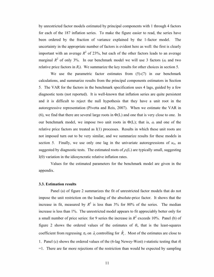
by unrestricted factor models estimated by principal components with 1 through 4 factors

for each of the 187 inflation series. To make the figure easier to read, the series have

been ordered by the fraction of variance explained by the 1-factor model. The

uncertainty in the appropriate number of factors is evident here as well: the first is clearly

important with an average R2 of 23%, but each of the other factors leads to an average

marginal R2 of only 3%. In our benchmark model we will use 3 factors (at and two

relative price factors in Rt). We summarize the key results for other choices in section 5.

We use the parametric factor estimates from (5)-(7) in our benchmark

calculations, and summarize results from the principal components estimators in Section

5. The VAR for the factors in the benchmark specification uses 4 lags, guided by a few

diagnostic tests (not reported). It is well-known that inflation series are quite persistent

and it is difficult to reject the null hypothesis that they have a unit root in the

autoregressive representation (Pivetta and Reis, 2007). When we estimate the VAR in

(6), we find that there are several large roots in Φ(L) and one that is very close to one. In

our benchmark model, we impose two unit roots in Φ(L); that is, at and one of the

relative price factors are treated as I(1) processes. Results in which these unit roots are

not imposed turn out to be very similar, and we summarize results for these models in

section 5. Finally, we use only one lag in the univariate autoregressions of uit, as

suggested by diagnostic tests. The estimated roots of ρi(L) are typically small, suggesting

I(0) variation in the idiosyncratic relative inflation rates.

Values for the estimated parameters for the benchmark model are given in the

appendix.

3.3. Estimation results

Panel (a) of figure 2 summarizes the fit of unrestricted factor models that do not

impose the unit restriction on the loading of the absolute-price factor. It shows that the

increase in fit, measured by R2 is less than 3% for 80% of the series. The median

increase is less than 1%. The unrestricted model appears to fit appreciably better only for

a small number of price series: for 9 series the increase in R2 exceeds 10%. Panel (b) of

figure 2 shows the ordered values of the estimates of θi, that is the least-squares

coefficient from regressing πit on ˆta controlling for ˆtR . Most of the estimates are close to

1. Panel (c) shows the ordered values of the (6-lag Newey-West) t-statistic testing that θi

=1. There are far more rejections of the restriction than would be expected by sampling

12

error, with over 30% of the t-statistics above the standard 5% critical values and over

20% above the 1% critical values. These results suggest that, as a formal matter, the unit

factor loading restriction in (2) appears to be rejected by the data. That said, the results in

panels (a) and (b) suggest that little is lost by imposing this restriction.

Figure 3 turns to the more interesting results: the maximum-likelihood estimates

of pure inflation. The figure plots estimates of υt as well the more familiar core PCE

inflation, and inflation in a representative sector, “major household appliances.” (The

figure shows 2-year changes of the inflation series because these are smoother and easier

to interpret than quarter-to-quarter changes.) Pure inflation is somewhat smoother than

the other two series, as well as less volatile (note the difference in the scales of the plots).

The standard deviation of Δυt is 0.40 percent, while that of core inflation changes is

1.26% and the median across the 87 price series is 5.8%.

Often, the three measures move together. For example, the two spikes in inflation

in the mid and late 1970s are common to all three measures of inflation. Likewise, the

disinflation of the early 1980s shows up both in core inflation as well as pure inflation,

and it is the largest contraction in pure inflation in the sample. In the 1990s, movements

in pure inflation do not match those in core PCE inflation. The disinflation of 1991-92 is

particularly pronounced in pure inflation, but not in core inflation and, in the late 1990s

and early 2000s, core inflation was low but pure inflation was particularly high.

4. Re-examining three classic macroeconomic correlations

In this section, we apply our estimates of pure inflation and relative-price changes

to answer three economic questions: how much of overall inflation is due to pure

inflation? What happens to the correlation between inflation and real activity once we

control for relative price changes? Are monetary policy variables closely linked to pure

inflation?

4.1 Inflation and pure inflation

Table 1 shows the fraction of the variability of overall inflation associated with

pure inflation, either averaged over all frequencies or just over business-cycle

frequencies. The first row of the table uses the PCE deflator as the measure of overall

inflation, and shows that roughly 15% of the movements in the series are accounted for

13

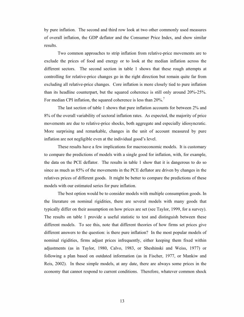
by pure inflation. The second and third row look at two other commonly used measures

of overall inflation, the GDP deflator and the Consumer Price Index, and show similar

results.

Two common approaches to strip inflation from relative-price movements are to

exclude the prices of food and energy or to look at the median inflation across the

different sectors. The second section in table 1 shows that these rough attempts at

controlling for relative-price changes go in the right direction but remain quite far from

excluding all relative-price changes. Core inflation is more closely tied to pure inflation

than its headline counterpart, but the squared coherence is still only around 20%-25%.

For median CPI inflation, the squared coherence is less than 20%.7

The last section of table 1 shows that pure inflation accounts for between 2% and

8% of the overall variability of sectoral inflation rates. As expected, the majority of price

movements are due to relative-price shocks, both aggregate and especially idiosyncratic.

More surprising and remarkable, changes in the unit of account measured by pure

inflation are not negligible even at the individual good’s level.

These results have a few implications for macroeconomic models. It is customary

to compare the predictions of models with a single good for inflation, with, for example,

the data on the PCE deflator. The results in table 1 show that it is dangerous to do so

since as much as 85% of the movements in the PCE deflator are driven by changes in the

relatives prices of different goods. It might be better to compare the predictions of these

models with our estimated series for pure inflation.

The best option would be to consider models with multiple consumption goods. In

the literature on nominal rigidities, there are several models with many goods that

typically differ on their assumption on how prices are set (see Taylor, 1999, for a survey).

The results on table 1 provide a useful statistic to test and distinguish between these

different models. To see this, note that different theories of how firms set prices give

different answers to the question: is there pure inflation? In the most popular models of

nominal rigidities, firms adjust prices infrequently, either keeping them fixed within

adjustments (as in Taylor, 1980, Calvo, 1983, or Sheshinski and Weiss, 1977) or

following a plan based on outdated information (as in Fischer, 1977, or Mankiw and

Reis, 2002). In these simple models, at any date, there are always some prices in the

economy that cannot respond to current conditions. Therefore, whatever common shock

14

affects desired prices, only some firms adjust their actual prices leading to a change in

relative prices. There is no pure inflation, because it is never the case that all firms

change their prices in exactly the same proportion at the same time. If the data we used

to estimate pure inflation were on goods prices, then our finding that there is pure

inflation would reject these simple models of nominal rigidities.

Our price data is on sectors though, not individual goods. The same logic as in

the previous paragraph applies as long as the extent of stickiness of prices is not exactly

the same in every sector. If price stickiness was identical in every sector, even though a

common shock to desired prices would lead to relative-price changes within sectors, there

would be no relative-price changes across sectors, and we would find pure inflation.

Away from this knife-edge case, strict models of nominal rigidities would still imply that

any common shock to desired prices would lead to relative-price changes and real effects,

but no pure inflation.8

More sophisticated models of nominal rigidities can generate movements in pure

inflation. For instance, in the imperfect-information model of Lucas (1972), changes in

the money supply that are announced ex ante are understood by all firms, so all change

their prices equiproportionately in response, leading to pure inflation. Likewise, in the

sticky-price model of Christiano, Eichenbaum and Evans (2005), where prices may be

indexed in between adjustments, it is possible to have movements in pure inflation. In

these models, in response to some shocks only some firms adjust leading to changes in

relative prices and real quantities, but in response to other shocks all prices adjust and

there is pure inflation. The proportion of price variability accounted for by pure inflation

provides a quantitative target with which to directly test the price adjustment mechanism

in these models.

In summary, simple models of sticky prices or information imply that there is no

pure inflation. Our findings reject these models. More sophisticated models of nominal

rigidities allow for pure inflation and their predictions on the size of the variance of pure

inflation relative to overall inflation are tightly linked to the assumptions on how prices

adjust to shocks. Our findings provide a statistic (15%-20%) to test these assumptions.

7 The series for median inflation is available from the Federal Reserve Bank of Cleveland from 1967:2 onwards. 8 It is also possible that in a finite sample, one might find some pure inflation even though in theory there should be none. Reis and Watson (2007) investigate this hypothesis by simulating data from simple sticky-price and sticky-information models with heterogeneous sectors. They find that, in these models, sampling uncertainty generates on average only between 2% and 7% fractions of inflation variability accounted for by pure inflation, well below our U.S. estimates.

15

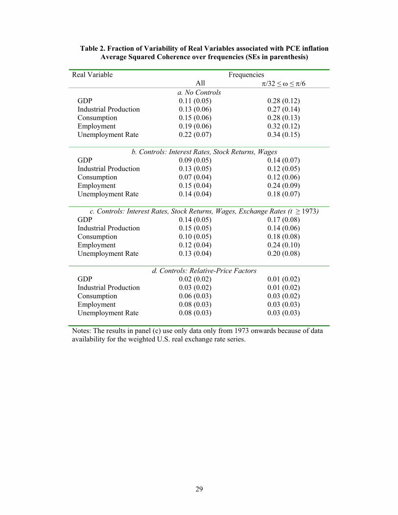
4.2 The Phillips correlation

One of the most famous correlations in macroeconomics, due to Phillips (1958),

relates changes in prices with measures of real activity. The first panel of table 2 displays

the Phillips correlation using our measures of squared coherence. At business-cycle

frequencies, measuring inflation with the PCE deflator and real activity with GDP, the

average squared coherence (R2) is 0.28, corresponding to a “correlation” of roughly 0.5.

The Phillips correlations for industrial production, consumption, employment or the

unemployment rate are all similarly large.

The second and third panels in table 2 show that the usual controls for relative

prices reduce the strength of this correlation. Controlling for intertemporal relative prices

(using short-term interest rates and stock returns), for the relative price of labor and

consumption (using real wages), or for the relative price of domestic and foreign goods

(using the real exchange rate) cuts the Phillips correlations in approximately half. Still,

these correlations remain quantitatively large and statistically significant at the 5% level.

The last panel of table 2 introduces as controls instead the measures of aggregate

relative-price movements that we estimated in this paper. Strikingly, the Phillips

correlation disappears over business cycle frequencies. The largest squared coherence

point estimate is 0.03 and the point estimates are statistically insignificant at the 10%

level for all measures of real activity.

As we saw earlier, the PCE deflator is a noisy measure of inflation, and this may

attenuate the Phillips correlation. Table 3 reassesses the Phillips correlations controlling

for goods’ relative prices by using instead our estimate of pure inflation. Panel (a) shows

the squared coherence between υt and the measures of real activity, and panels (b) and (c)

add the additional controls associated with real wages, asset prices and exchange rates.

Evidently, the correlation of the real variables and pure inflation is much smaller than

their correlation with the PCE deflator (the squared coherences fall by a factor of roughly

two-thirds).

The results in these tables suggest that a large part of the Phillips correlation, that

has puzzled macroeconomists for half a century, is driven by changes in good’s relative

prices. Changes in the unit of account, as captured by pure inflation, do not seem to

affect real variables, consistent with the absence of money illusion. However, note that a

few of the estimates in table 3 are statistically significant, even if small. This suggests

that some money illusion may be present, although it seems to explain very little of the

16

variability of real activity.

4.3 Pure inflation and monetary policy

Another famous set of correlations in empirical macroeconomics are between

measures of monetary policy and inflation. Friedman and Schwartz (1963) famously

observed that in the long run, money growth and inflation are tightly linked. Equally

famously, Fisher (1930) and many that followed showed that there is an almost as strong

link between nominal interest rates and inflation in the long run. At business-cycle

frequencies though, these correlations are much weaker. The correlation between money

growth and inflation is unstable and typically low (Stock and Watson, 1999), while the

correlation between inflation and nominal interest rates is typically higher, but well

below its level at lower-frequencies (Mishkin, 1992).

Table 4 reproduces the findings described in the previous paragraph for different

measures of money growth (M0, M1, and M2) and different short-term nominal interest

rates (the federal funds rate and the 3-month Treasury bill rate), measuring inflation using

the PCE deflator. The growth rate of M0 and M1 is very weakly correlated with the PCE

deflator, and while the relation with M2 is stronger, it is imprecisely estimated. The link

between inflation and nominal interest rates is stronger, in particular at business-cycle

frequencies.

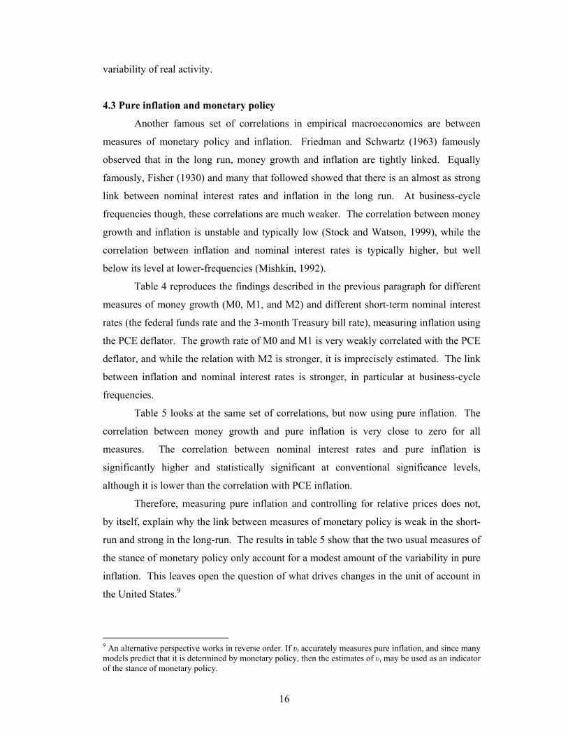
Table 5 looks at the same set of correlations, but now using pure inflation. The

correlation between money growth and pure inflation is very close to zero for all

measures. The correlation between nominal interest rates and pure inflation is

significantly higher and statistically significant at conventional significance levels,

although it is lower than the correlation with PCE inflation.

Therefore, measuring pure inflation and controlling for relative prices does not,

by itself, explain why the link between measures of monetary policy is weak in the short-

run and strong in the long-run. The results in table 5 show that the two usual measures of

the stance of monetary policy only account for a modest amount of the variability in pure

inflation. This leaves open the question of what drives changes in the unit of account in

the United States.9

9 An alternative perspective works in reverse order. If υt accurately measures pure inflation, and since many models predict that it is determined by monetary policy, then the estimates of υt may be used as an indicator of the stance of monetary policy.

17

5. The robustness of the results

Table 6 investigates the robustness of the key empirical conclusions to four

aspects of the model specification: (i) the number of estimated factors, (ii) the method for

estimating the factors (signal extraction using the parametric factor model (5)-(7) versus

principal components on (4)), (iii) the imposition of unit roots in the factor VAR for the

parametric model, and (iv) the number of lags and imposition of unit roots in the VAR

spectral estimator used to compute the various coherence estimates.

The first row of the table shows results for the benchmark model, where the first

column provides details of the factor estimates and where “(1,1,0)” denotes a parametric

k=3 factor model where the first and second factor are I(1) processes and the third is I(0).

The next column, labeled “VAR”, summarizes the specification of the VAR used to

compute the spectral estimates, which for the benchmark model involves 4 lags of first

differences (D,4) of υt and, for the final two columns, first differences of money growth

and interest rates. The next set of results are for factor models estimated using the

parametric model, but with different numbers of factors and/or I(0) specifications for the

first two factors. Results are shown for spectral estimates computed using the first-

difference VAR and for a VAR computed using the level of υt and, for the final two

columns, the level of money growth and nominal interest rates. The final rows of the

table show results for factors computed using principal components. The numerical

entries in the table are the average squared coherence of the estimate of υt with the

variable listed in column heading (in the case of real GDP, controlling for interest rates,

stock returns and wages as in the panel (b) of table 3).

Looking across the entries in the table, two results stand out. First, the

quantitative conclusions concerning the correlation of υt with aggregate inflation (core

PCE in the table), real output (real GDP in the table) and monetary policy indicators (M2

and the nominal Federal Funds rate in the table) appear to be quite robust across the

different specifications. Second, the various estimates of υt based on the parametric

model are highly correlated with the estimates from the benchmark model, but the

estimates based on principal components are less so. The R2 measures relating the

principal components estimates of υt and the benchmark estimates range from 0.38 to

0.66, suggesting correlations in the range of 0.6 to 0.8. Figure 4 shows the estimates of

υt−υt−8 from the benchmark model (this is the same series plotted in figure 3) and the

principal components estimates constructed from the corresponding 3-factor model.

18

While the two series evolve similarly (their correlation is 0.65), there are some obvious

differences. Our interpretation of these differences is that, despite their shared large N,T

consistency properties, there is some gain from exploiting the time series averaging used

in the parametric model that is ignored in the principal components estimator. In any

event, despite the differences in the two sets of estimates for pure inflation, their

implications for the macroeconomic correlations summarized in the remaining columns

of the table are similar.

6. What have we done and why does it matter?

In this paper, we decomposed the quarterly change in sectoral goods’ prices into

three components: pure inflation, aggregate relative prices, and idiosyncratic relative

prices. We used different estimation techniques and specifications to robustly estimate

pure inflation, and proposed a simple method to compute macroeconomic correlations

while controlling for goods’ relative price changes.

Our first finding was that pure inflation can differ markedly from other

conventional measures of inflation, like the PCE deflator or its core version. It is

smoother, less volatile, and in particular in the 1990s, its ups-and-downs are quite

different from those in other measures of inflation. This should be useful to economic

historians since it provides an alternative account of the movements in inflation in the last

half-century. Relative to existing measure of inflation, pure inflation has the virtue of

separating absolute from relative-price changes, which is a crucial distinction in

economic theory. Moreover, pure inflation matches more closely the concept that many

economists seem to have in mind when discussing aggregate movements in prices and

monetary policy (typically based on intuition that comes from a one-good world).

Our second main finding was that pure inflation was quantitatively significant (it

accounts for about 5% of individual price changes), but only accounts for 15-20% of the

variability in inflation measured by conventional price indices, like the PCE deflator, the

GDP deflator, or the CPI. This has at least two implications for the work of economic

theorists building models to explain inflation. First, it shows that comparing the

predictions of one-good models with common measures of inflation is flawed. The

difference between these measures and pure inflation is large enough that it can easily

lead to mistakenly accepting or rejecting models. Second, our estimates provide a new

test statistic with which to test the pricing assumptions of models with many goods. An

19

important ingredient (and topic of debate) in recent models of nominal rigidities is a

model of pricing that implies slow adjustment of prices to monetary policy shocks

together with frequent price changes. The fraction of the variability of cost-of-living

inflation accounted for by pure inflation can be an important statistic to diagnose the

success of these models at fitting the data.

Third, we found that, once we controlled for relative goods’ prices, the Phillips

correlation became quantitatively insignificant. Therefore, the correlation between real

quantity variables and nominal inflation variables that we observe in the data can be

accounted for by changes in relative prices. This implies that models that break the

classical dichotomy via nominal rigidities in good’s price adjustment are likely more

promising than models that rely on money illusion on the part of agents.

Fourth, we found that pure inflation is partly related to monetary policy variables.

The link to the growth rate in monetary aggregates is weak, but the correlation with

nominal interest rates at business cycle frequencies is strong (approximately 0.5).

To conclude, economic theories have strong predictions on whether and when

there should be pure inflation and what its effects would be, and discussions of monetary

policy often revolve around its relation with pure inflation. However, observing pure

inflation is naturally difficult, since the concept itself is more a fruit of thought

experiments than something easily observed. As a result, there have been few systematic

attempts to measure it in the data. The goal of this paper was to make some progress on

measuring pure inflation and understanding its effects. Our estimates are certainly not

perfect. We hope, however, that they are sufficiently accurate that future research can

look deeper into the time-series and the moments that we provide, and that by stating the

challenges and putting forward a benchmark, we can motivate future research to come up

with better estimators. Likewise, we are sure that our findings will not settle the debates

around the key macroeconomic correlations. Our more modest hope is that they offer a

new perspective on how to bring data to bear on these long-standing questions.

20

References

Altissimo, Filippo, Benoit Mojon, and Paolo Zaffaroni (2006). “Fast Micro and Slow

Macro: Can Aggregation Explain the Persistence of Inflation?” Manuscript, Federal

Reserve Bank of Chicago.

Amstad, Marlene and Simon M. Potter (2007). “Real Time Underlying Inflation Gauges

for Monetary Policy Makers.” Manuscript, Federal Reserve Bank of Chicago.

Bai, Jushan (2003). “Inferential Theory for Factor Models of Large Dimensions.”

Econometrica, vol. 71 (1), pp. 135-171.

Bai, Jushan and Serena Ng (2002). “Determining the Number of Factors in Approximate

Factor Models.” Econometrica, vol. 70 (1), pp. 191-221.

Bai, Jusham and Serena Ng (2006). “Confidence Intervals for Diffusion Index Forecasts

and Inference for Factor Augmented Regressions.” Econometrica, 74:4, p. 1133-

1150.

Bernanke, Ben , Jean Boivin and Piotr S. Eliasz (2005). “Measuring the Effects of

Monetary Policy: A Factor-augmented Vector Autoregressive (FAVAR) Approach.”

Quarterly Journal of Economics, vol. 120 (1), pp. 387-422.

Boivin, Jean, Marc Giannoni and Ilian Mihov (2007). “Sticky Prices and Monetary

Policy: Evidence from Disaggregated Data.” NBER working paper 12824.

Broda, Christian and David Weinstein (2007). “Product Creation and Destruction:

Evidence and Price Implications” NBER working paper 13041.

Bryan, Michael F. and Stephen G. Cecchetti (1993). “The Consumer Price Index as a

Measure of Inflation.” Federal Reserve Bank of Cleveland Economic Review, pp. 15-

24.

Bryan, Michael F., Stephen G. Cecchetti and Rodney L. Wiggins II (1997). “Efficient

Inflation Estimation.” NBER working paper 6183.

Calvo, Guillermo (1983). “Staggered Prices in a Utility-Maximizing Framework.”

Journal of Monetary Economics, vol. 12, pp. 383-398.

Christiano, Lawrence J., Martin Eichenbaum, and Charles S. Evans (2005). “Nominal

Rigidities and the Dynamic Effects of a Shock to Monetary Policy.” Journal of

Political Economy, vol. 113 (1), pp. 1-45.

Cristadoro, Riccardo, Mario Forni, Lucrezia Reichlin and Giovanni Veronese (2005). “A

Core Inflation Index for the Euro Area.” Journal of Money, Credit and Banking, vol.

37 (3), pp. 539-560.

21

Del Negro, Marco (2006). “Signal and Noise in Core PCE.” presentation, Federal

Reserve Bank of Atlanta, June 2006.

Doz, Catherine, Domenico Giannone and Lucrezia Reichlin (2006). “A Quasi Maximum

Likelihood Approach for Large Dynamic Factor Models.” CEPR discussion paper

5724.

Fischer, Stanley (1977). “Long-Term Contracts, Rational Expectations, and the Optimal

Money Supply Rule.” Journal of Political Economy, vol. 85 (1), pp. 191-205.

Fisher, Irving (1930). The Theory of Interest. MacMillan, New York.

Forni, Mario, Marc Hallin, Marco Lippi, and Lucrezia Reichlin (2000). “The Generalized

Dynamic Factor Model: Identification and Estimation.” Review of Economics and

Statistics, vol. 82 (4), pp. 540-554.

Friedman, Milton and Anna J. Schwartz (1963). A Monetary History of the United States.

Princeton: Princeton University Press.

Hamilton, James D. (1993). Time Series Analysis, Princeton: Princeton University Press.

Hume, David (1752). Political Discourses. Reprinted in “Essays, Moral, Political, and

Literary” edited by Eugene F. Miller, Liberty Fund.

Lucas, Robert E., Jr. (1972). “Expectations and the Neutrality of Money.” Journal of

Economic Theory, vol. (4), pp. 103-124.

Mankiw, N. Gregory and Ricardo Reis (2002). “Sticky Information versus Sticky Prices:

A Proposal to Replace the New Keynesian Phillips Curve.” Quarterly Journal of

Economics, vol. 117 (4), pp. 1295-1328.

Mishkin, Frederic S. (1992). “Is the Fisher Effect for Real? A Reexamination of the

Relationship between Inflation and Interest Rates.” Journal of Monetary Economics,

vol. 30 (2), pp. 195-215.

Phillips, Alban W. H. (1958). “The Relation between Unemployment and the Rate of

Change of Money Wage Rates in the United Kingdom, 1861-1957.” Economica, vol.

25 (2), pp. 283-299.

Pivetta, Frederic and Ricardo Reis (2007). “The Persistence of Inflation in the United

States.” Journal of Economic Dynamics and Control, vol. 31 (4), pp. 1326-1358.

Quah, Danny and Thomas J. Sargent (1993). “A Dynamic Index Model for Large Cross-

Sections.” In James H. Stock and Mark W. Watson, eds., Business Cycles, Indicators,

and Forecasting, pp. 161–200, Chicago: University of Chicago Press and NBER.

Reis, Ricardo and Mark W. Watson (2007) “Measuring Changes in the Value of the

Numeraire.” Manuscript, Princeton University.

22

Selvanathan, E. A. and D. S. Prasada Rao (1994). Index Numbers: A Stochastic

Approach. Michigan: University of Michigan Press.

Sheshinski, Eytan and Yoram Weiss (1977). “Inflation and Costs of Price Adjustment.”

Review of Economic Studies, vol. 44 (2), pp. 287-303.

Shumway, Robert H. and David S. Stoffer (1982). “An Approach to Time Series

Smoothing and Forecasting using the EM Algorithm.” Journal of Time Series

Analysis, vol. 2, pp. 253-264.

Stock, James H. and Mark W. Watson (1989). “New Indexes of Leading and Coincident

Indicators.” In Olivier J. Blanchard and Stanley Fischer, eds., NBER Macroeconomics

Annual 1989, pp. 351-394.

Stock, James H. and Mark W. Watson (1999). “Business Cycle Fluctuations in U.S.

Macroeconomic Time Series.” In John B. Taylor and Michael Woodford, eds.,

Handbook of Macroeconomics, Elsevier..

Stock, James H. and Mark W. Watson (2002). “Forecasting Using Principal

Components from a Large Number of Predictors.” Journal of the American

Statistical Association, vol. 97, 1167-1179.

Stock, James H. and Mark W. Watson (2005). “Implications of Dynamic Factor Models

for VAR Analysis.” NBER working paper 11467.

Taylor, John B. (1980). “Aggregate Dynamics and Staggered Contracts.” Journal of

Political Economy, vol. 88 (1), pp. 1-24.

Taylor, John B. (1999). “Staggered Price and Wage Setting in Macroeconomics.” In John

B. Taylor and Michael Woodford, Handbook of Macroeconomics, Elsevier.

Watson, Mark W. (1989). “Recursive Solution Methods for Dynamic Linear Rational

Expectations Models.” Journal of Econometrics, vol. 41, pp. 65-91.

Watson, Mark W. and Robert F. Engle (1983). “Alternative Algorithms for the

Estimation of Dynamic Factors, MIMIC, and Varying Coefficient Regression

models.” Journal of Econometrics, vol. 23, pp. 385-400.

23

Appendix

All price series are from NIPA Table 2.4.4U available from

http://www.bea.gov/national/nipaweb/nipa_underlying/SelectTable.asp. Quarterly inflation rates were computed using the first difference of logarithms of the price indices for the last month of the quarter. Inflation observations that differed from the series median by more that six times the interquartile range were replaced by the local median computed using the six adjacent observations. The table below shows the price index from the NIPA table, the series description, the standard deviation of the (outlier-adjusted) series over 1959:2-2006:2 and the 2005 PCE expenditure share. To save space, the final four columns of this table are used to show the estimated parameters from the benchmark 3-factor model.

Table A1: Series Descriptions, Summary Statistics, and Parameter Estimates from the Benchmark 3-factor Model

Benchmark Model ParametersNum.

Label Description sπ 2005

Share λ1 λ2 ρ σe 001 P1NFCG D New foreign autos 4.5 0.5 1.14 0.00 -0.13 0.88 002 P1NETG D Net transactions in used autos 1.8 0.4 2.35 0.42 0.15 2.71 003 P1MARG D Used auto margin 6.9 0.3 1.09 0.18 0.02 4.22 004 P1REEG D Employee reimbursement 7.5 0.0 1.11 0.15 -0.19 1.68 005 P1TRUG D Trucks, new and net used 4.8 2.4 1.25 -0.09 -0.12 0.96 006 P1TATG D Tires and tubes 5.8 0.3 0.15 0.57 0.12 1.27 007 P1PAAG D Accessories and parts 5.5 0.4 -0.21 -0.04 0.26 1.15 008 P1FNRG C Furniture, incl. matt. and bedsprings 4.1 0.9 0.53 0.30 -0.29 0.77 009 P1MHAG D Major household appliances 4.0 0.4 0.84 0.13 0.09 0.73 010 P1SEAG D Small electric appliances 5.0 0.1 1.06 0.35 0.12 0.93 011 P1CHNG C China, glassware, tableware, and utensil 6.7 0.4 1.32 0.93 -0.28 1.25 012 P1TVSG D Television receivers 5.4 0.2 1.16 0.47 0.42 0.99 013 P1AUDG D Audio equipment 5.2 0.3 0.57 0.06 -0.17 1.17 014 P1RTDG D Records, tapes, and disks 4.9 0.2 -0.21 0.07 -0.06 1.17 015 P1MSCG D Musical instruments 4.0 0.1 0.41 0.22 -0.13 0.85 016 P1FLRG D Floor coverings 5.8 0.2 0.60 0.09 -0.24 1.27 017 P1CLFG D Clocks, lamps, and furnishings 6.0 0.4 1.22 0.45 -0.04 1.29 018 P1TEXG D Blinds, rods, and other 8.6 0.1 1.54 1.07 -0.28 1.81 019 P1WTRG D Writing equipment 5.1 0.0 0.18 -1.01 -0.28 1.06 020 P1HDWG D Tools, hardware, and supplies 4.7 0.1 0.56 0.14 -0.04 1.05 021 P1LWNG D Outdoor equipment and supplies 5.1 0.0 0.73 0.13 -0.16 1.11 022 P1OPTG C Ophth. prd, and orthopedic appliances 2.8 0.3 0.29 -0.05 -0.07 0.55 023 P1CAMG D Photographic equipment 6.0 0.1 1.26 0.04 0.34 1.25 024 P1BCYG D Bicycles 4.3 0.1 -0.09 0.30 -0.15 0.90 025 P1MCYG D Motorcycles 4.7 0.2 1.18 -0.11 0.01 1.00 026 P1AIRG D Pleasure aircraft 7.2 0.0 0.05 0.57 0.06 1.64 027 P1JRYG C Jewelry and watches (18) 7.3 0.7 0.15 0.33 -0.21 1.67 028 P1BKSG C Books and maps (87) 5.8 0.5 1.00 -0.37 -0.25 1.23 029 P1GRAG D Cereals 6.3 0.4 -1.34 -0.19 0.45 1.34 030 P1BAKG D Bakery products 4.6 0.6 -0.22 0.25 0.14 1.01 031 P1BEEG D Beef and veal 13.0 0.4 -4.16 -0.28 -0.16 2.88 032 P1PORG D Pork 6.9 0.3 -3.52 -0.91 0.19 3.96 033 P1MEAG D Other meats 8.3 0.2 -2.72 -0.74 0.17 1.84 034 P1POUG D Poultry 7.0 0.5 -2.23 0.03 -0.20 4.06 035 P1FISG D Fish and seafood 5.7 0.2 -0.69 0.01 0.18 1.22 036 P1GGSG D Eggs 7.4 0.1 -5.34 -0.42 -0.03 6.63 037 P1MILG D Fresh milk and cream 6.9 0.2 -1.10 0.04 -0.03 1.63 038 P1DAIG D Processed dairy products 6.2 0.5 -1.19 0.08 0.28 1.32 039 P1FRUG D Fresh fruits 4.5 0.3 -0.89 0.21 -0.07 3.55 040 P1VEGG D Fresh vegetables 9.3 0.4 -2.70 -0.21 -0.41 6.59 041 P1PFVG D Processed fruits and vegetables 5.7 0.2 0.40 0.15 0.38 1.21 042 P1JNBG D Juices and nonalcoholic drinks 6.4 0.8 0.16 0.64 0.32 1.22 043 P1CTMG D Coffee, tea and beverage materials 1.8 0.2 1.49 0.89 0.58 2.31 044 P1FATG D Fats and oils 9.3 0.1 -0.60 1.33 0.52 1.71 045 P1SWEG D Sugar and sweets 6.3 0.5 -0.97 0.36 0.27 1.37 046 P1OFDG D Other foods 4.1 1.3 0.11 0.05 0.11 0.76

24

047 P1PEFG D Pet food 3.9 0.3 -0.19 0.04 -0.04 0.79 048 P1MLTG D Beer and ale, at home 3.6 0.7 0.42 0.18 0.13 0.66 049 P1WING D Wine and brandy, at home 3.9 0.2 -0.51 0.14 -0.02 0.79 050 P1LIQG D Distilled spirits, at home 2.1 0.2 -0.17 -0.40 0.25 0.54 051 P1OPMG D Other purchased meals 2.8 4.5 -0.15 0.09 0.30 0.32 052 P1APMG C Alcohol in purchased meals 3.7 0.6 0.45 -0.06 -0.16 0.79 053 P1MFDG D Food supplied military 3.0 0.0 -0.20 0.10 0.25 0.40 054 P1FFDG C Food produced and consumed on farms 0.9 0.0 -4.86 -1.37 -0.09 4.98 055 P1SHUG C Shoes (12) 3.8 0.6 -0.01 0.41 0.01 0.78 056 P1WGCG D Clothing for females 4.5 1.8 -0.14 0.30 0.02 1.10 057 P1WICG D Clothing for infants 8.9 0.1 1.40 0.58 -0.33 1.88 058 P1MBCG D Clothing for males 3.5 1.2 0.30 0.34 0.11 0.74 059 P1MSGG D Sewing goods for males 6.4 0.0 0.28 0.25 -0.29 1.46 060 P1MUGG D Luggage for males 2.6 0.0 1.29 1.25 -0.21 2.82 061 P1MICG C Std. clothing issued to military personnel 2.8 0.0 0.28 0.16 0.15 0.43 062 P1GASG D Gasoline and other motor fuel 4.2 3.2 -6.30 1.54 -0.13 5.37 063 P1LUBG D Lubricants 5.5 0.0 -0.37 0.47 0.37 1.09 064 P1OILG D Fuel oil 3.7 0.1 -7.75 2.55 0.21 4.84 065 P1FFWG D Farm fuel 6.0 0.0 -3.91 1.84 0.14 3.38 066 P1TOBG C Tobacco products 7.5 1.0 0.36 -0.70 0.06 1.83 067 P1SOAG D Soap 4.9 0.1 1.21 0.25 -0.13 0.92 068 P1CSMG D Cosmetics and perfumes 4.3 0.2 1.07 0.17 -0.24 0.78 069 P1SDHG C Semidurable house furnishings 7.4 0.5 1.76 0.64 -0.44 1.40 070 P1CLEG D Cleaning preparations 4.2 0.4 0.66 0.13 0.09 0.75 071 P1LIGG D Lighting supplies 7.2 0.1 0.87 0.53 -0.13 1.59 072 P1PAPG D Paper products 5.6 0.3 0.36 0.40 0.04 1.17 073 P1RXDG D Prescription drugs 4.0 2.6 0.33 -0.62 0.67 0.55 074 P1NRXG D Nonprescription drugs 4.0 0.3 0.91 -0.45 0.10 0.64 075 P1MDSG D Medical supplies 3.7 0.1 0.77 -0.58 -0.13 0.64 076 P1GYNG D Gynecological goods 4.2 0.0 1.02 0.24 -0.08 0.68 077 P1DOLG D Toys, dolls, and games 5.4 0.6 1.04 0.47 0.10 1.08 078 P1AMMG D Sport supplies, including ammunition 4.7 0.2 0.35 0.15 -0.16 1.06 079 P1FLMG D Film and photo supplies 4.6 0.0 0.62 -0.25 0.10 1.06 080 P1STSG D Stationery and school supplies 4.7 0.1 0.91 0.50 -0.04 0.95 081 P1GREG D Greeting cards 4.8 0.1 0.92 0.50 -0.04 0.97 082 P1ABDG C Expenditures abroad by U.S. residents 16.8 0.1 0.28 0.54 0.18 4.02 083 P1MGZG D Magazines and sheet music 5.5 0.3 0.66 -0.44 -0.31 1.17 084 P1NWPG D Newspapers 3.8 0.2 0.87 0.24 0.14 0.78 085 P1FLOG C Flowers, seeds, and potted plants 6.7 0.2 0.57 0.29 -0.12 1.54 086 P1OMHG D Owner occupied mobile homes 2.5 0.4 0.03 -0.74 -0.30 0.24 087 P1OSTG D Owner occupied stationary homes 2.4 10.7 0.00 -0.75 -0.17 0.19 088 P1TMHG D Tenant occupied mobile homes 3.8 0.1 0.07 -0.75 -0.26 0.77 089 P1TSPG D Tenant occupied stationary homes 2.4 2.8 -0.04 -0.77 -0.31 0.17 090 P1TLDG D Tenant landlord durables 3.8 0.1 0.45 -0.51 0.25 0.66 091 P1FARG C Rental value of farm dwellings (26) 4.3 0.2 -0.27 -0.15 0.70 0.84 092 P1HOTG D Hotels and motels 6.3 0.6 0.19 -0.01 -0.10 1.38 093 P1HFRG D Clubs and fraternity housing 2.9 0.0 0.03 -0.65 -0.33 0.43 094 P1HHEG D Higher education housing 3.0 0.2 -0.15 -0.78 0.04 0.54 095 P1HESG D El. and secondary education housing 8.9 0.0 0.16 -0.84 -0.36 2.01 096 P1TGRG D Tenant group room and board 3.4 0.0 -0.12 -0.70 -0.38 0.60 097 P1ELCG C Electricity (37) 5.7 1.5 0.43 -0.16 0.23 1.15 098 P1NGSG C Gas (38) 2.6 0.8 0.35 0.19 0.44 2.71 099 P1WSMG D Water and sewerage maintenance 3.9 0.6 0.88 -0.50 0.20 0.75 100 P1REFG D Refuse collection 4.1 0.2 1.02 -0.56 0.29 0.75 101 P1LOCG D Local and cellular telephone 4.5 1.3 0.41 -0.84 0.05 0.98 102 P1OLCG D Local telephone 4.4 0.6 0.05 -1.00 0.00 1.00 103 P1LDTG D Long distance telephone 5.3 0.3 0.15 -0.31 0.33 1.24 104 P1INCG D Intrastate toll calls 5.1 0.1 -0.08 -0.66 0.36 1.17 105 P1ITCG D Interstate toll calls 6.3 0.2 0.38 0.09 0.23 1.52 106 P1DMCG D Domestic service, cash 4.3 0.2 0.27 0.10 0.24 0.98 107 P1DMIG D Domestic service, in kind 6.0 0.0 -1.76 -0.21 -0.03 1.24 108 P1MSEG D Moving and storage 3.7 0.2 0.15 0.09 -0.03 0.69 109 P1FIPG D Household insurance premiums 3.7 0.2 0.13 -0.49 0.32 0.84 110 P1FIBG D Less: Household insurance benefits paid 3.3 0.1 0.86 0.38 -0.28 0.40 111 P1RCLG D Rug and furniture cleaning 4.4 0.0 0.33 0.06 -0.36 0.79 112 P1EREG D Electrical repair 3.8 0.1 0.06 0.12 0.17 0.79 113 P1FREG D Reupholstery and furniture repair 3.2 0.0 -0.11 -0.20 0.13 0.74 114 P1MHOG D Household operation services, n.e.c. 3.7 0.2 0.03 0.09 -0.02 0.73 115 P1ARPG D Motor vehicle repair 2.9 1.7 0.17 0.06 0.30 0.34 116 P1RLOG D Motor vehicle rental, leasing, and other 4.9 0.6 0.82 0.15 -0.16 0.96 117 P1TOLG C Bridge, tunnel, ferry, and road tolls 6.2 0.1 0.00 -0.75 -0.19 1.42

25

118 P1AING C Insurance 4.2 0.7 0.84 -0.73 0.13 3.61 119 P1IMTG C Mass transit systems 5.4 0.1 0.09 -0.45 0.09 1.35 120 P1TAXG C Taxicab 5.7 0.0 0.05 0.22 0.02 1.27 121 P1IBUG C Bus 9.2 0.0 -0.10 -0.37 -0.20 2.13 122 P1IAIG C Airline 15.0 0.4 -0.64 0.75 -0.04 3.60 123 P1TROG C Other 9.1 0.1 -0.23 -0.04 -0.05 2.11 124 P1PHYG C Physicians 3.3 4.0 0.63 -0.09 0.50 0.42 125 P1DENG C Dentists 2.7 1.0 0.39 -0.22 0.17 0.48 126 P1OPSG C Other professional services 3.2 2.7 0.61 0.04 0.25 0.50 127 P1NPHG C Nonprofit 3.1 4.4 0.05 -0.02 0.03 0.48 128 P1GVHG C Government 4.3 1.4 -0.10 -0.06 0.51 0.76 129 P1NRSG C Nursing homes 3.3 1.3 0.05 0.11 -0.30 0.62 130 P1MING C Medical care and hospitalization 0.3 1.4 -0.90 -0.95 0.29 4.89 131 P1IING C Income loss 5.7 0.0 0.70 -1.74 0.64 4.86 132 P1PWCG C Workers' compensation 8.1 0.2 -0.55 0.26 0.80 1.16 133 P1MOVG C Motion picture theaters 4.1 0.1 0.05 0.08 0.15 1.07 134 P1LEGG C Leg. theaters and opera, 4.2 0.1 0.13 0.11 0.16 1.10 135 P1SPEG C Spectator sports 4.1 0.2 -0.15 -0.34 -0.08 1.03 136 P1RTVG C Radio and television repair 3.1 0.1 0.28 -0.52 0.33 0.62 137 P1CLUG C Clubs and fraternal organizations 4.2 0.3 -0.13 0.42 -0.27 0.77 138 P1SIGG D Sightseeing 5.3 0.1 0.04 0.00 -0.07 1.21 139 P1FLYG D Private flying 9.8 0.0 0.48 0.19 -0.28 2.27 140 P1BILG D Bowling and billiards 4.1 0.0 0.46 -0.31 0.05 0.96 141 P1CASG D Casino gambling 2.9 0.9 -0.28 0.10 -0.22 0.32 142 P1OPAG D Other com. participant amusements 2.8 0.3 0.27 0.06 0.16 0.59 143 P1PARG C Pari-mutuel net receipts 4.8 0.1 -0.66 -0.09 0.51 0.99 144 P1PETG D Pets and pets services excl. vet. 3.6 0.1 -0.12 -0.07 0.00 0.76 145 P1VETG D Veterinarians 3.0 0.2 -0.18 -0.23 0.13 0.67 146 P1CTVG D Cable television 7.0 0.7 0.18 -0.21 0.08 1.76 147 P1FDVG D Film developing 3.8 0.1 0.76 -0.08 0.39 0.85 148 P1PICG D Photo studios 3.8 0.1 0.12 -0.12 0.09 0.89 149 P1CMPG D Sporting and recreational camps 3.4 0.0 0.09 -0.04 -0.07 0.81 150 P1HREG D High school recreation 4.7 0.0 0.05 -0.14 -0.22 1.12 151 P1NECG D Commercial amusements n.e.c. 3.4 0.6 0.25 0.00 -0.05 0.80 152 P1NISG D Com. amusements n.e.c. except ISPs 3.3 0.4 0.12 -0.05 -0.04 0.80 153 P1SCLG D Shoe repair 3.3 0.0 0.04 -0.27 0.12 0.64 154 P1DRYG D Drycleaning 3.6 0.1 0.30 0.18 0.24 0.52 155 P1LGRG D Laundry and garment repair 3.6 0.1 -0.03 0.07 0.12 0.57 156 P1BEAG D Beauty shops, including combination 3.9 0.5 0.08 -0.09 0.17 0.76 157 P1BARG D Barber shops 2.8 0.0 0.01 0.08 0.11 0.56 158 P1WCRG D Watch, clock, and jewelry repair 3.3 0.0 -0.01 -0.30 -0.03 0.66 159 P1CRPG D Miscellaneous personal services 3.8 0.5 0.17 0.11 -0.02 0.62 160 P1BROG C Brokerage charges and inv. couns. 1.2 1.0 0.30 0.50 0.01 5.18 161 P1BNKG C Bnk srv. chges, trust serv., s-d box rental 5.7 1.2 1.81 -0.70 0.39 1.02 162 P1IMCG D Commercial banks 2.4 1.0 -0.18 0.76 0.18 2.93 163 P1IMNG D Other financial institutions 15.0 1.4 0.19 -0.32 0.58 3.05 164 P1LIFG C Exp. of handl. life ins. and pension plans 2.3 1.2 -0.37 -0.24 0.49 0.45 165 P1GALG C Legal services (65) 4.4 1.0 0.60 -0.41 0.14 0.91 166 P1FUNG C Funeral and burial expenses 3.2 0.2 0.47 -0.61 0.35 0.57 167 P1UNSG D Labor union expenses 4.1 0.2 -0.32 0.29 0.07 0.74 168 P1ASSG D Profession association expenses 6.5 0.1 -0.23 0.03 -0.37 1.33 169 P1GENG D Employment agency fees 5.5 0.0 1.40 -0.11 -0.04 1.03 170 P1AMOG D Money orders 5.3 0.0 1.12 -0.24 -0.21 1.09 171 P1CLAG D Classified ads 5.4 0.0 1.15 -0.23 -0.16 1.09 172 P1ACCG D Tax return preparation services 5.2 0.1 0.97 -0.31 -0.11 1.12 173 P1THEG D Personal business services, n.e.c. 7.1 0.1 0.61 -0.55 -0.03 1.66 174 P1PEDG D Private higher education 4.4 0.7 -0.25 -0.13 0.02 0.89 175 P1GEDG D Public higher education 4.1 0.7 0.52 -0.27 0.07 0.89 176 P1ESCG D Elementary and secondary schools 4.3 0.4 -0.47 0.20 -0.02 0.84 177 P1NSCG D Nursery schools 4.8 0.1 -0.63 0.01 0.02 1.05 178 P1VEDG D Commercial and vocational schools 4.1 0.4 -0.96 -0.38 0.20 0.88 179 P1REDG D Foundations and nonprofit research 4.5 0.2 -0.37 -0.27 -0.03 1.05 180 P1POLG D Political organizations 8.2 0.0 0.04 0.39 -0.32 1.83 181 P1MUSG D Museums and libraries 5.7 0.1 -0.70 0.08 -0.13 1.18 182 P1FOUG D Foundations to religion and welfare 5.4 0.2 -0.54 0.09 0.01 1.11 183 P1WELG D Social welfare 3.3 1.7 -0.39 0.12 -0.01 0.54 184 P1RELG D Religion 5.0 0.7 0.17 0.19 -0.09 1.11 185 P1AFTG D Passenger fares for foreign travel 9.8 0.5 -0.95 0.39 -0.08 2.32 186 P1USTG D U.S. travel outside the U.S. 9.6 0.6 -2.04 0.50 0.15 2.16 187 P1FTUG D Foreign travel in U.S. 3.6 1.0 -0.20 0.00 0.04 0.62

26

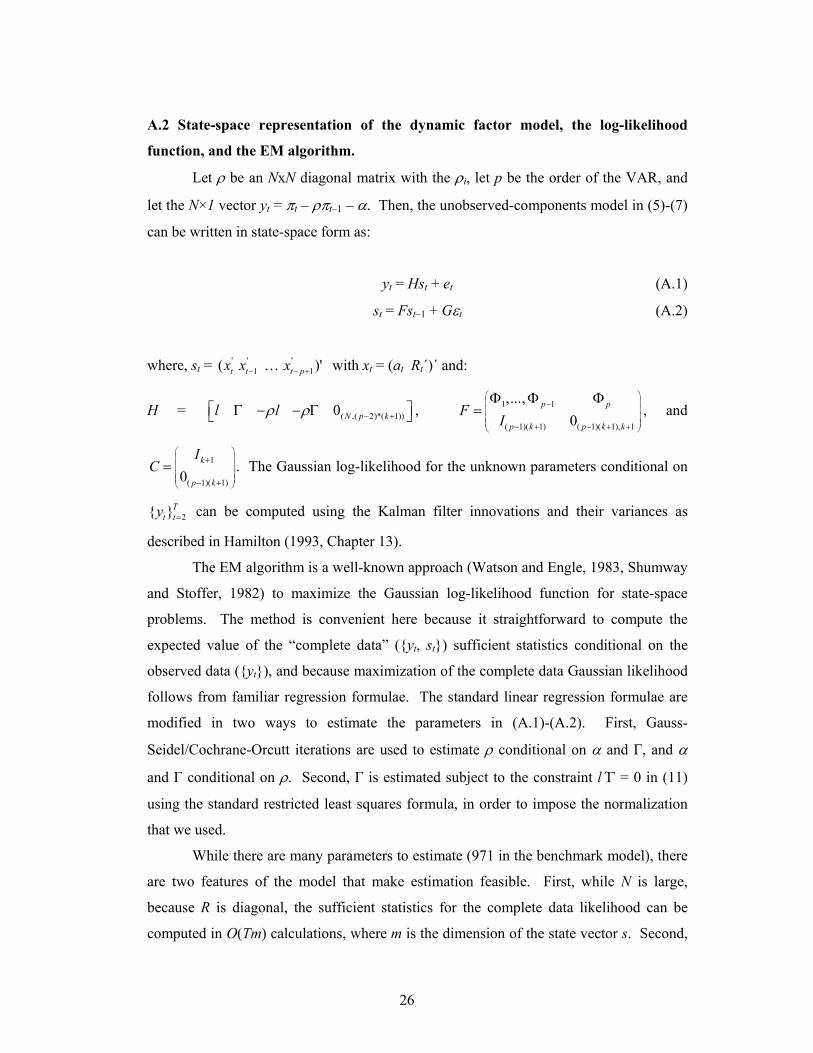
A.2 State-space representation of the dynamic factor model, the log-likelihood

function, and the EM algorithm.

Let ρ be an NxN diagonal matrix with the ρi, let p be the order of the VAR, and

let the N×1 vector yt = πt – ρπt–1 – α. Then, the unobserved-components model in (5)-(7)

can be written in state-space form as:

yt = Hst + et (A.1)

st = Fst–1 + Gεt (A.2)

where, st = ' ' '1 1( )' t t t px x x− − +… with xt = (at Rt´)´ and:

H = ( ,( 2)*( 1)) 0 N p kl lρ ρ − +⎡ ⎤Γ − − Γ⎣ ⎦ , 1 1

( 1)( 1) ( 1)( 1) 10p p

p k p k k

FI

⎛ ⎞⎜ ⎟−⎜ ⎟⎜ ⎟⎜ ⎟− + − + , +⎝ ⎠

Φ ,...,Φ Φ= , and

1

( 1)( 1)0k

p k

IC

⎛ ⎞⎜ ⎟+⎜ ⎟⎜ ⎟⎜ ⎟− +⎝ ⎠

= . The Gaussian log-likelihood for the unknown parameters conditional on

2{ }Tt ty = can be computed using the Kalman filter innovations and their variances as

described in Hamilton (1993, Chapter 13).

The EM algorithm is a well-known approach (Watson and Engle, 1983, Shumway

and Stoffer, 1982) to maximize the Gaussian log-likelihood function for state-space

problems. The method is convenient here because it straightforward to compute the

expected value of the “complete data” ({yt, st}) sufficient statistics conditional on the

observed data ({yt}), and because maximization of the complete data Gaussian likelihood

follows from familiar regression formulae. The standard linear regression formulae are

modified in two ways to estimate the parameters in (A.1)-(A.2). First, Gauss-

Seidel/Cochrane-Orcutt iterations are used to estimate ρ conditional on α and Γ, and α

and Γ conditional on ρ. Second, Γ is estimated subject to the constraint l´Γ = 0 in (11)

using the standard restricted least squares formula, in order to impose the normalization

that we used.

While there are many parameters to estimate (971 in the benchmark model), there

are two features of the model that make estimation feasible. First, while N is large,

because R is diagonal, the sufficient statistics for the complete data likelihood can be

computed in O(Tm) calculations, where m is the dimension of the state vector s. Second,

27

because N and T are large, the principal component estimators of (at Rt´) are reasonably

accurate and regression based estimators of the model parameters can be constructed

using these estimates of the factors. These principal component based estimates serve as

useful initial values for the MLE algorithm. (See Doz, Giannone and Reichlin, 2006, for

further discussion.) Results reported in the text are based on 40,000 EM iterations,

although results using 5,000 iterations are essentially identical.

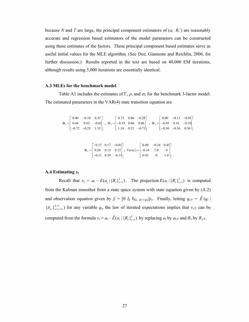
A.3 MLEs for the benchmark model

Table A1 includes the estimates of Γ, ρ, and σe for the benchmark 3-factor model.

The estimated parameters in the VAR(4) state transition equation are

1

0.40 0.10 0.350.44 0.63 0.010.72 0.25 1.33

−⎡ ⎤⎢ ⎥Φ = −⎢ ⎥⎢ ⎥− −⎣ ⎦

, 2

0.73 0.06 0.280.19 0.06 0.06

1.14 0.21 0.71

−⎡ ⎤⎢ ⎥Φ = −⎢ ⎥⎢ ⎥−⎣ ⎦

, 2

0.00 0.13 0.050.45 0.16 0.100.30 0.36 0.36

− −⎡ ⎤⎢ ⎥Φ = − −⎢ ⎥⎢ ⎥− −⎣ ⎦

4

0.13 0.17 0.010.20 0.15 0.120.11 0.39 0.11

− −⎡ ⎤⎢ ⎥Φ = ⎢ ⎥⎢ ⎥− −⎣ ⎦

, 0.40 0.16 0.45

( ) 0.16 1.0 00.45 0 1.0

Var ε−⎡ ⎤

⎢ ⎥= −⎢ ⎥⎢ ⎥⎣ ⎦

A.4 Estimating υt

Recall that υt = at – 1( |{ } )TtE a Rτ τ = . The projection 1( |{ } )T

tE a Rτ τ = is computed

from the Kalman smoother from a state space system with state equation given by (A.2)

and observation equation given by ft = [0 Ik 0(k, (k+1)p)]st. Finally, letting qt/T = E (qt | ,1, 1{ }N T

i iτ τπ = = ) for any variable qt, the law of iterated expectations implies that vt/T can be

computed from the formula vt = at – 1ˆ ( |{ } )T

tE a Rτ τ = by replacing at by at/T and Rτ by Rτ/T.

28

Table 1. Fraction of Variability of Inflation associated with Pure Inflation

Average Squared Coherence over frequencies (SEs in parentheses)

Inflation measure Frequencies

All π/32 ≤ ω ≤ π/6

Usual Measures

Headline PCE 0.16 (0.04) 0.15 (0.07)

Headline GDP 0.21 (0.04) 0.15 (0.07)

Headline CPI 0.12 (0.03) 0.15 (0.06)

Available Pure Measures

Core PCE 0.24 (0.05) 0.21 (0.09)

Median CPI 0.14 (0.04) 0.18 (0.08)

187 Sectoral Inflation Rates

25th Percentile 0.03 0.02

Median 0.05 0.05

75th Percentile 0.07 0.08

Notes: PCE is the Personal Consumption Expenditures deflator, GDP is the Gross Domestic Product deflator, and CPI is the Consumer Price Index. Median CPI inflation is from the Federal Reserve Bank of Cleveland and these data are are available for t ≥ 1967:2. For the last panel, we computed the fraction of variability explained by pure inflation for each of the 187 goods’ series, and report the 25%, 50%, and 75% values.

29

Table 2. Fraction of Variability of Real Variables associated with PCE inflation Average Squared Coherence over frequencies (SEs in parenthesis)

Frequencies Real Variable

All π/32 ≤ ω ≤ π/6 a. No Controls

GDP 0.11 (0.05) 0.28 (0.12) Industrial Production 0.13 (0.06) 0.27 (0.14) Consumption 0.15 (0.06) 0.28 (0.13) Employment 0.19 (0.06) 0.32 (0.12) Unemployment Rate 0.22 (0.07) 0.34 (0.15)

b. Controls: Interest Rates, Stock Returns, Wages

GDP 0.09 (0.05) 0.14 (0.07) Industrial Production 0.13 (0.05) 0.12 (0.05) Consumption 0.07 (0.04) 0.12 (0.06) Employment 0.15 (0.04) 0.24 (0.09) Unemployment Rate 0.14 (0.04) 0.18 (0.07)

c. Controls: Interest Rates, Stock Returns, Wages, Exchange Rates (t ≥ 1973)

GDP 0.14 (0.05) 0.17 (0.08) Industrial Production 0.15 (0.05) 0.14 (0.06) Consumption 0.10 (0.05) 0.18 (0.08) Employment 0.12 (0.04) 0.24 (0.10) Unemployment Rate 0.13 (0.04) 0.20 (0.08)

d. Controls: Relative-Price Factors

GDP 0.02 (0.02) 0.01 (0.02) Industrial Production 0.03 (0.02) 0.01 (0.02) Consumption 0.06 (0.03) 0.03 (0.02) Employment 0.08 (0.03) 0.03 (0.03) Unemployment Rate 0.08 (0.03) 0.03 (0.03) Notes: The results in panel (c) use only data only from 1973 onwards because of data availability for the weighted U.S. real exchange rate series.

30

Table 3. Fraction of Variability of Real Variables associated with Pure Inflation Average Squared Coherence over frequencies (SEs in parenthesis)

Frequencies Real Variable

All π/32 ≤ ω ≤ π/6 a. No Controls

GDP 0.05 (0.02) 0.09 (0.05) Industrial Production 0.06 (0.02) 0.09 (0.06) Consumption 0.08 (0.03) 0.08 (0.04) Employment 0.07 (0.02) 0.12 (0.06) Unemployment Rate 0.12 (0.03) 0.13 (0.07)

b. Controls: Interest Rates, Stock Returns, Wages

GDP 0.04 (0.02) 0.05 (0.03) Industrial Production 0.05 (0.02) 0.04 (0.02) Consumption 0.05 (0.02) 0.06 (0.03) Employment 0.06 (0.02) 0.10 (0.04) Unemployment Rate 0.12 (0.03) 0.07 (0.03)

c. Controls: Interest Rates, Stock Returns, Wages, Exchange Rates (t ≥ 1973)

GDP 0.03 (0.02) 0.07 (0.04) Industrial Production 0.04 (0.02) 0.04 (0.03) Consumption 0.04 (0.02) 0.06 (0.04) Employment 0.06 (0.02) 0.16 (0.07) Unemployment Rate 0.10 (0.02) 0.09 (0.05) Notes: The results in panel (c) use only data only from 1973 onwards because of data availability for the weighted U.S. real exchange rate series.

31

Table 4. Monetary Policy and PCE Inflation Average Squared Coherence over frequencies (SEs in parenthesis)

Frequencies Monetary variable

All π/32 ≤ ω ≤ π/6 Money growth M0 0.05 (0.03) 0.03 (0.04) M1 0.02 (0.02) 0.02 (0.03) M2 0.10 (0.04) 0.16 (0.10)

Nominal Interest Rate Federal Funds Rate 0.14 (0.05) 0.41 (0.14) 3-Month T-bill Rate 0.12 (0.05) 0.33 (0.15)

Table 5. Monetary Policy and Pure Inflation Average Squared Coherence over frequencies (SEs in parenthesis)

Frequencies Monetary variable

All π/32 ≤ ω ≤ π/6 Money growth M0 0.04 (0.02) 0.01 (0.02) M1 0.06 (0.03) 0.01 (0.02) M2 0.03 (0.02) 0.01 (0.02)

Nominal Interest Rate Federal Funds Rate 0.11 (0.04) 0.27 (0.10) 3-Month T-bill Rate 0.12 (0.03) 0.27 (0.12)

32

Table 6. Robustness of Results to Model Specification Average Squared Coherence over business cycle frequencies (SEs in parenthesis)

Factor

Estimates VAR ˆBenchmark

tυ Core PCE Inflation

Real GDP

Money (M2)

Interest Rate (FFR)

Benchmark Model (1,1,0) D,4 1.00 0.21 (.09) 0.05 (0.03) 0.01 (0.02) 0.27 (0.10)

Using Alternative Parametric Factor Estimates (1,1,0) D,6 1.00 0.15 (0.06) 0.06 (0.03) 0.06 (0.07) 0.20 (0.09) (0,0,0) D,4 1.00 0.22 (0.09) 0.05 (0.03) 0.01 (0.02) 0.30 (0.11) (0,0,0) D,6 0.99 0.15 (0.06) 0.06 (0.03) 0.05 (0.07) 0.20 (0.09) (1,1,0,0) D,4 0.95 0.21 (0.09) 0.05 (0.03) 0.01 (0.01) 0.21 (0.10) (1,1,0,0) D,6 0.91 0.15 (0.06) 0.07 (0.04) 0.05 (0.06) 0.15 (0.09) (1,1,0) L,4 1.00 0.18 (0.07) 0.09 (0.04) 0.02 (0.03) 0.20 (0.11) (1,1,0) L,6 1.00 0.15 (0.07) 0.11 (0.04) 0.03 (0.05) 0.20 (0.11) (0,0,0) L,4 0.99 0.16 (0.06) 0.09 (0.04) 0.02 (0.03) 0.19 (0.11) (0,0,0) L,6 1.00 0.14 (0.06) 0.10 (0.04) 0.03 (0.05) 0.19 (0.11) (1,1,0,0) L,4 0.90 0.19 (0.07) 0.08 (0.04) 0.02 (0.03) 0.24 (0.10) (1,1,0,0) L,6 0.86 0.15 (0.07) 0.11 (0.04) 0.03 (0.04) 0.22 (0.10)

Using Principal Component Factor Estimates PC-3 D,4 0.46 0.35 (0.13) 0.02 (0.02) 0.00 (0.01) 0.30 (0.12) PC-3 D,6 0.49 0.25 (0.09) 0.02 (0.01) 0.06 (0.06) 0.28 (0.10) PC-4 D,4 0.54 0.33 (0.12) 0.02 (0.02) 0.01 (0.02) 0.36 (0.10) PC-4 D,6 0.56 0.22 (0.08) 0.03 (0.02) 0.08 (0.06) 0.33 (0.09) PC-2 D,4 0.43 0.49 (0.15) 0.01 (0.01) 0.00 (0.01) 0.30 (0.13) PC-2 D,6 0.40 0.30 (0.10) 0.03 (0.02) 0.06 (0.06) 0.29 (0.10) PC-3 L,4 0.61 0.18 (0.07) 0.09 (0.04) 0.01 (0.01) 0.15 (0.09) PC-3 L,6 0.54 0.16 (0.07) 0.04 (0.02) 0.05 (0.07) 0.16 (0.09) PC-4 L,4 0.66 0.17 (0.06) 0.04 (0.02) 0.00 (0.01) 0.26 (0.10) PC-4 L,6 0.65 0.13 (0.06) 0.05 (0.03) 0.07 (0.07) 0.24 (0.10) PC-2 L,4 0.43 0.29 (0.10) 0.02 (0.02) 0.02 (0.04) 0.18 (0.10) PC-2 L,6 0.38 0.21 (0.08) 0.05 (0.04) 0.04 (0.06) 0.21 (0.11) Notes: The first column describes the factor estimates, where the parametric estimates are based on signal extraction applied to (5)-(7) with parameters estimated by Gaussian MLE, and the numbers in parenthesis indicate the number of factors and whether the relevant factor is modeled as an I(1) or I(0) process. For example, “(1,1,0)” is a three factor model modeled as I(1), I(1), and I(0) processes. PC-k denotes a k-factor model estimated by principal components. The column labeled VAR shows the specification of the VAR used to compute the VAR-spectral estimates, where “D” and “L” denote first differences and levels specifications and the numbers 4 and 6 denote the number of lags in the VAR.

33

Figure 1. Choosing the number of factors

Panel a) Eigenvalues of the correlation matrix

0

5

10

15

20

25

30

35

40

45

1 2 3 4 5 6 7 8 9 10 11 12 13 14 15 16 17 18 19 20

Panel b) Contribution of more factors to the R2 of each good

0

0.1

0.2

0.3

0.4

0.5

0.6

0.7

0.8

0.9

k = 1 k = 2 k = 3 k = 4 Notes: Panel a) shows the eigenvalues of the N×N sample correlation matrix of inflation rates. Panel b) shows the fraction of sample variance of inflation explained by k factors, where k varies from k=1 to k=4.

34

Figure 2. Comparison with unrestricted factor model

Panel a) Increase in R2 from moving to unrestricted model

0

0.05

0.1

0.15

0.2

0.25

Panel b) Estimates of θi, the coefficient on absolute-price component

-2

-1

0

1

2

3

4

Panel c) Individual t-statistics for hypothesis θi=1

-8

-6

-4

-2

0

2

4

6

Notes: The horizontal axis in each panel goes from i = 1 to i = 187. In each panel, the goods are organized in increasing order.

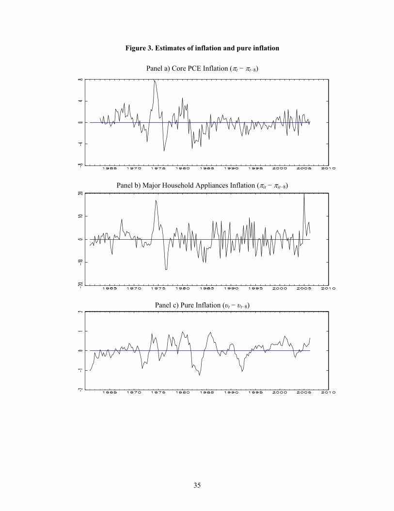
35

Figure 3. Estimates of inflation and pure inflation

Panel a) Core PCE Inflation (πt − πt−8)

Panel b) Major Household Appliances Inflation (πit − πit−8)

Panel c) Pure Inflation (υt − υt−8)

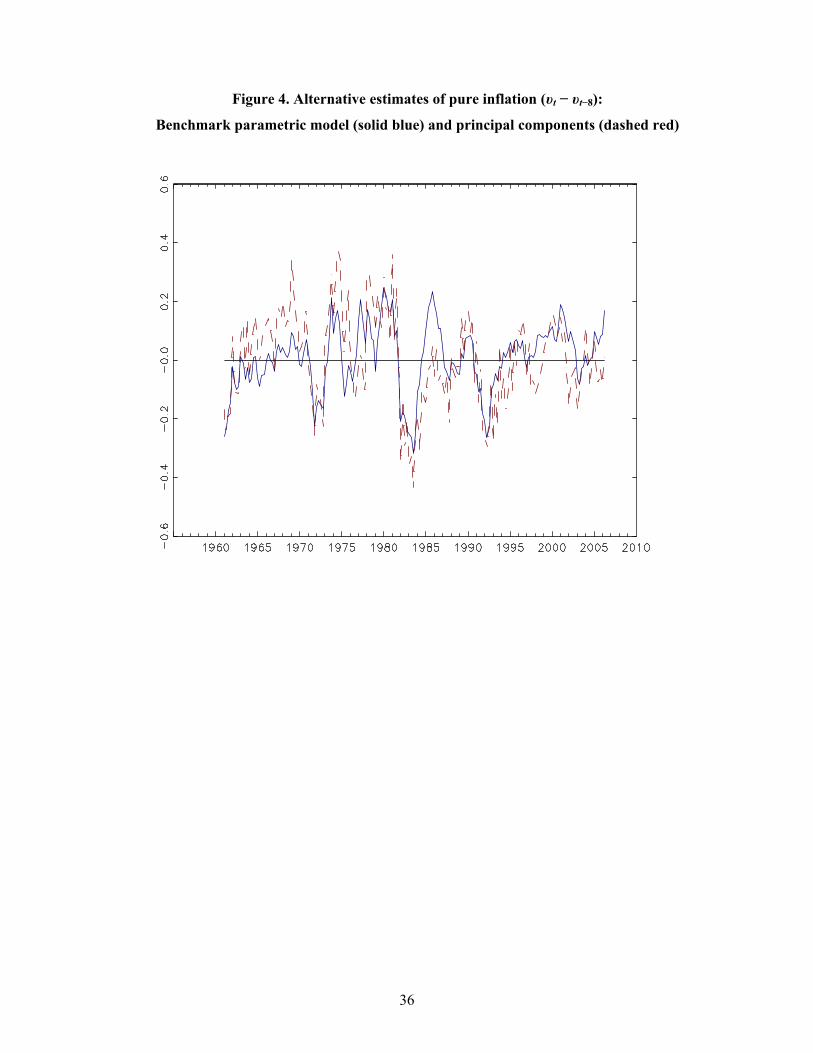
36

Figure 4. Alternative estimates of pure inflation (υt − υt−8):

Benchmark parametric model (solid blue) and principal components (dashed red)