Embed Size (px)
Citation preview
Relationship between Morphology and Terrestrial and Aquatic Invertebrate Assemblages:
A case study at the Bünz (CH)
Master thesis by Christina Baumgartner October 2008 Supervisor: Dr. Christopher T. Robinson


Master thesis by:
Christina Baumgartner
Bruggerstrasse 57
5400 Baden
Supervised by: PD Dr. Christopher T. Robinson, Eawag Dübendorf
1. Examiner: PD Dr. Christopher T. Robinson, Eawag Dübendorf
2. Examiner: Prof. Dr. Klement Tockner, IGB Berlin
submitted at:
Überlandstrasse 133 Department of Biology
8600 Dübendorf 8092 Zürich

Contents
1 Summary .............................................................................................................1
2 Introduction .........................................................................................................3
3 Material and Methods .........................................................................................5
3.1 Study system................................................................................................5
3.2 Study sites....................................................................................................5
3.3 Morphological measurements.......................................................................9
3.3.1 Ecomorphology .......................................................................................9
3.3.2 Indicators ................................................................................................9
3.3.3 Vegetation measurements ....................................................................10
3.4 Biotic measurements ..................................................................................11
3.5 Analysis of data ..........................................................................................14
4 Results ...............................................................................................................15
4.1 Morphology.................................................................................................15
4.2 Biotic assemblages.....................................................................................18
4.2.1 Abundance and diversity.......................................................................18
4.2.2 Correlations...........................................................................................24
4.3 Correlations between morphology and invertebrates .................................24
5 Discussion.........................................................................................................26 5.1 Morphology.................................................................................................26
5.2 Biotic assemblages.....................................................................................28
5.2.1 Abundance and diversity.......................................................................28
5.2.2 Correlations between aquatic and terrestrial communities....................29
5.3 Correlations between morphology and invertebrates .................................30
5.3.1 Aquatic communities.............................................................................30
5.3.2 Terrestrial communities.........................................................................31
5.4 Conclusions ................................................................................................32
6 Acknowledgements ..........................................................................................33
7 References ........................................................................................................34
Index of Figures
Figure 1: The seven study sites along the Bünz......................................................5
Figure 2: Schematic overview of the study design ..................................................6
Figure 3: Site FP .....................................................................................................6
Figure 4: Site NN.....................................................................................................7
Figure 5: Site DG ....................................................................................................7
Figure 6: Site R1 .....................................................................................................7
Figure 7: Site R2 .....................................................................................................8
Figure 8: Site R3 .....................................................................................................8
Figure 9: Site R4 .....................................................................................................8
Figure 10: Schematic overview of the sampling methods .....................................11
Figure 11: Discharge during sampling surveys .....................................................12
Figure 12: The different trap types ........................................................................13
Figure 13: Means of indicator values for each site ................................................15
Figure 14: PCA plot...............................................................................................17
Figure 15: Results of biotic measurements ...........................................................19
Figure 16: Results of biotic measurements ...........................................................20
Figure 17: Results of biotic measurements ...........................................................21
Figure 18: Results of biotic measurements ...........................................................22
Figure 19: Results of biotic measurements ...........................................................23
Figure 20: Correlation between emergence and riparian predators ......................24
Figure 21: Correlation between morphological and biological parameters............25

Index of Tables
Table 1: Summary of morphological measurements .............................................16
Table 2: Output from the PCA analysis .................................................................17
Table 3: ANOVA table ...........................................................................................18
Summary ___________________________________
1
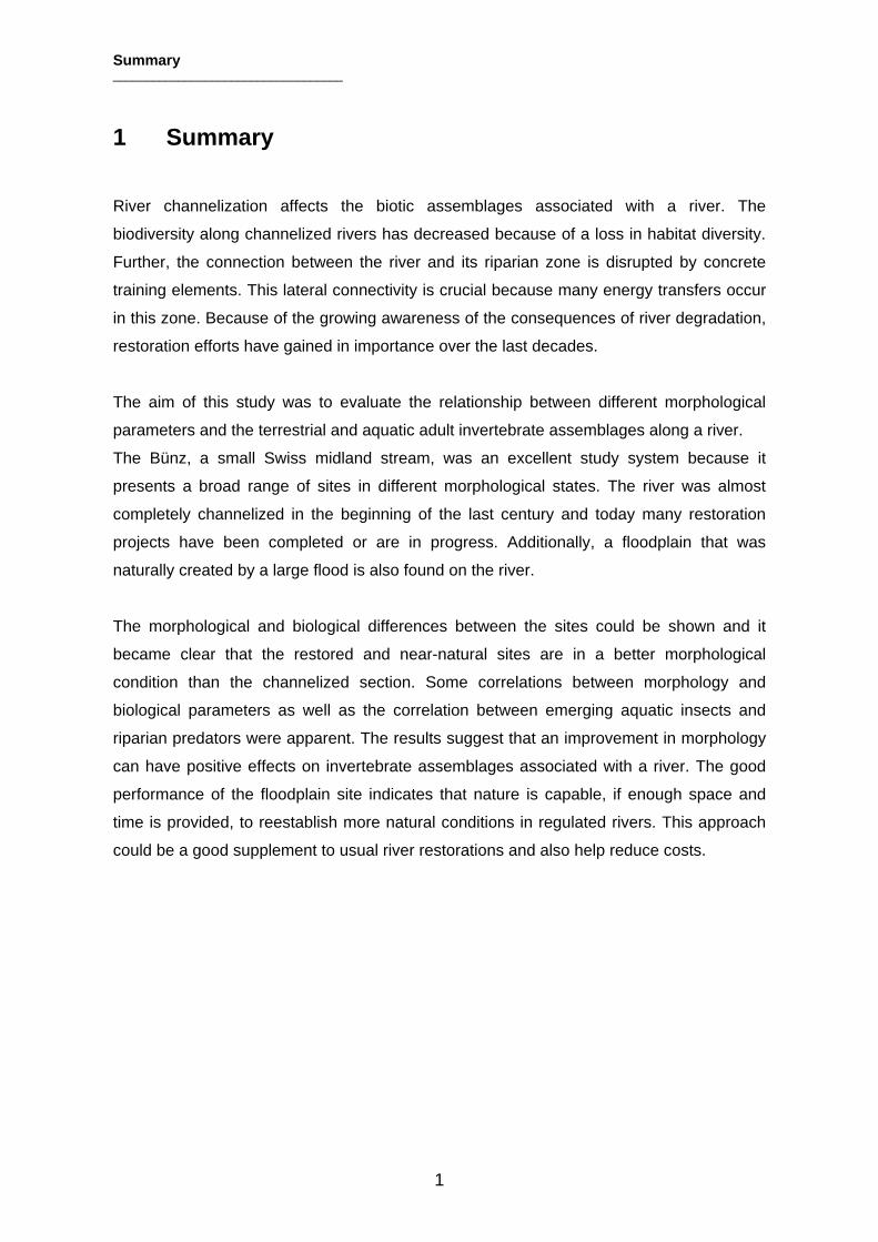
1 Summary
River channelization affects the biotic assemblages associated with a river. The
biodiversity along channelized rivers has decreased because of a loss in habitat diversity.
Further, the connection between the river and its riparian zone is disrupted by concrete
training elements. This lateral connectivity is crucial because many energy transfers occur
in this zone. Because of the growing awareness of the consequences of river degradation,
restoration efforts have gained in importance over the last decades.
The aim of this study was to evaluate the relationship between different morphological
parameters and the terrestrial and aquatic adult invertebrate assemblages along a river.
The Bünz, a small Swiss midland stream, was an excellent study system because it
presents a broad range of sites in different morphological states. The river was almost
completely channelized in the beginning of the last century and today many restoration
projects have been completed or are in progress. Additionally, a floodplain that was
naturally created by a large flood is also found on the river.
The morphological and biological differences between the sites could be shown and it
became clear that the restored and near-natural sites are in a better morphological
condition than the channelized section. Some correlations between morphology and
biological parameters as well as the correlation between emerging aquatic insects and
riparian predators were apparent. The results suggest that an improvement in morphology
can have positive effects on invertebrate assemblages associated with a river. The good
performance of the floodplain site indicates that nature is capable, if enough space and
time is provided, to reestablish more natural conditions in regulated rivers. This approach
could be a good supplement to usual river restorations and also help reduce costs.
Summary ___________________________________
2
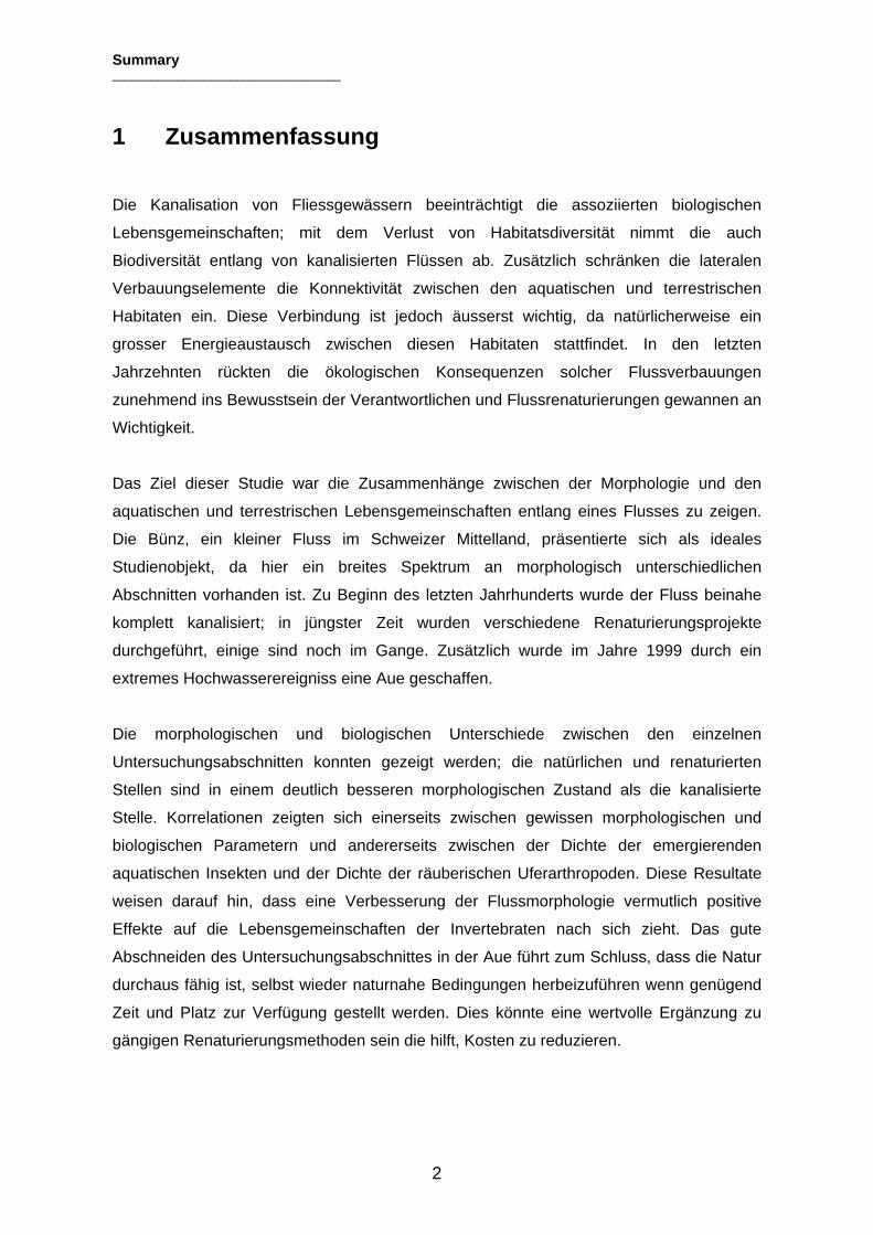
1 Zusammenfassung
Die Kanalisation von Fliessgewässern beeinträchtigt die assoziierten biologischen
Lebensgemeinschaften; mit dem Verlust von Habitatsdiversität nimmt die auch
Biodiversität entlang von kanalisierten Flüssen ab. Zusätzlich schränken die lateralen
Verbauungselemente die Konnektivität zwischen den aquatischen und terrestrischen
Habitaten ein. Diese Verbindung ist jedoch äusserst wichtig, da natürlicherweise ein
grosser Energieaustausch zwischen diesen Habitaten stattfindet. In den letzten
Jahrzehnten rückten die ökologischen Konsequenzen solcher Flussverbauungen
zunehmend ins Bewusstsein der Verantwortlichen und Flussrenaturierungen gewannen an
Wichtigkeit.
Das Ziel dieser Studie war die Zusammenhänge zwischen der Morphologie und den
aquatischen und terrestrischen Lebensgemeinschaften entlang eines Flusses zu zeigen.
Die Bünz, ein kleiner Fluss im Schweizer Mittelland, präsentierte sich als ideales
Studienobjekt, da hier ein breites Spektrum an morphologisch unterschiedlichen
Abschnitten vorhanden ist. Zu Beginn des letzten Jahrhunderts wurde der Fluss beinahe
komplett kanalisiert; in jüngster Zeit wurden verschiedene Renaturierungsprojekte
durchgeführt, einige sind noch im Gange. Zusätzlich wurde im Jahre 1999 durch ein
extremes Hochwasserereigniss eine Aue geschaffen.
Die morphologischen und biologischen Unterschiede zwischen den einzelnen
Untersuchungsabschnitten konnten gezeigt werden; die natürlichen und renaturierten
Stellen sind in einem deutlich besseren morphologischen Zustand als die kanalisierte
Stelle. Korrelationen zeigten sich einerseits zwischen gewissen morphologischen und
biologischen Parametern und andererseits zwischen der Dichte der emergierenden
aquatischen Insekten und der Dichte der räuberischen Uferarthropoden. Diese Resultate
weisen darauf hin, dass eine Verbesserung der Flussmorphologie vermutlich positive
Effekte auf die Lebensgemeinschaften der Invertebraten nach sich zieht. Das gute
Abschneiden des Untersuchungsabschnittes in der Aue führt zum Schluss, dass die Natur
durchaus fähig ist, selbst wieder naturnahe Bedingungen herbeizuführen wenn genügend
Zeit und Platz zur Verfügung gestellt werden. Dies könnte eine wertvolle Ergänzung zu
gängigen Renaturierungsmethoden sein die hilft, Kosten zu reduzieren.

Introduction ___________________________________
3
2 Introduction
Natural river corridors consist of diverse landscape elements and therefore provide a
broad range of different habitats (Ward et al., 2002). This heterogeneity leads to high
levels of biodiversity in riverine landscapes (Ward, 1998). Unfortunately, almost all river
corridors in Europe were regulated before the science of river ecology was developed
(Ward et al., 2001). We now know that alterations in river morphology can have
widespread impacts to associated habitats (Paetzold et al., 2005). Channelization and
stabilization of riverbanks affect the connection between the river and the riparian zone.
The resulting disruption of these two habitats has severe impacts on aquatic and terrestrial
biotic communities along the river.
In the last decades, society began addressing the ecological consequences from the
degradation of many riverine ecosystems. Interest in stream restoration has increased and
many projects have been or are being completed, and developed for the future (Lake et al.,
2007). Additionally, public awareness of ecological processes occurring in rivers has
increased, and responsible stakeholders are switching from solely engineering solutions to
ecologically-based activities (Palmer et al., 2005). For example, the awareness of lateral
connectivity has gained in importance and riparian zones are now integrated part of river
ecosystems and thus considered in planning river restorations (Lake et al., 2007).
Following Naiman et al., (1993), natural riparian zones are among the most diverse and
dynamic biophysical ecotonal habitats. They consist of a diverse mosaic of landforms and
act as an interface between terrestrial and aquatic biotopes. Numerous aquatic-terrestrial
interactions, including crucial energy flows, occur in this zone. Aquatic and terrestrial
invertebrate communities along a river are interdependent and the change in abundance
on one side can directly influence the other (Marczak and Richardson, 2007). Rivers and
their riparian zones are closely linked by reciprocal flows of invertebrate prey (Baxter et al.,
2005), and the largest part of the riparian fauna is predaceous (Hering and Plachter, 1997).
Predation by riparian arthropods, e.g. ground-dwelling beetles on emerging insects, is an
important pathway of energy transfer from aquatic to terrestrial foodwebs (Paetzold et al.,
2005; Iwata, 2007). Reciprocally, the input of terrestrial arthropods, via in-fall and drift,
transfers terrestrial energy to aquatic habitats, for example, as prey for fish (Allan et al.,
2003).
Introduction ___________________________________
4
In this study, terrestrial and aquatic adult invertebrate assemblages were investigated
along a river with sites of different morphological condition. The aim of the study was,
firstly, to show the morphological differences between natural, human-affected and
restored sites. Further, terrestrial and aquatic adult invertebrate assemblages were
examined at these sites and then relations between emergence, riparian predators and
terrestrial inputs were identified, and correlations between morphological and biotic
parameters tested.
The following hypotheses were tested:
I: The ecomorphological state will differ between the different sites. Sites affected by
human activities will be in a worse morphological state than natural or restored sites.
II: Differences between sites and season will be apparent in the terrestrial and aquatic
adult invertebrate assemblages.
III: There will be a relationship between the emergence of aquatic insects, riparian
predators, and input of terrestrial invertebrates into the river at the different sites.
IV: Measured biotic parameters will correlate with the morphological characteristics of the
different sites.
Material and Methods ___________________________________
5
3 Material and Methods
3.1 Study system
The River Bünz is a small midland stream about 25 km
long and has a yearly average discharge of ca.1.5 m3/s at
Othmarsingen. In its natural state, it was a slow
meandering river due to the low slope. Because it required
large areas that were periodically flooded, a large length of
the river was channelized around 1930 to claim space for
agriculture and human settlement. Only a part of the
downstream section was left in a near-natural state. In this
part, the riverbanks were stabilized to keep the river in its
channel. In the last five years, multiple restoration projects
were completed along the river in the formerly channelized
part. In the near natural section, an extreme flood event
created a floodplain in the year 1999 (Burger, 2007). A
small hydropower plant that is privately owned
hydrologically influences the downstream part of the river
by periodic releases.
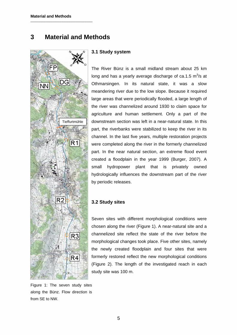
3.2 Study sites
Seven sites with different morphological conditions were
chosen along the river (Figure 1). A near-natural site and a
channelized site reflect the state of the river before the
morphological changes took place. Five other sites, namely
the newly created floodplain and four sites that were
formerly restored reflect the new morphological conditions
(Figure 2). The length of the investigated reach in each
study site was 100 m.
Figure 1: The seven study sites
along the Bünz. Flow direction is
from SE to NW.
Tieffurtmühle
Material and Methods ___________________________________
6
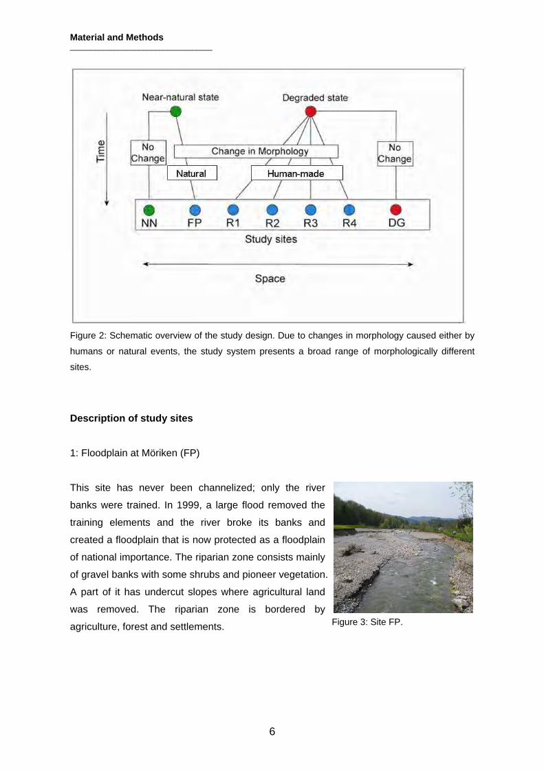
Figure 2: Schematic overview of the study design. Due to changes in morphology caused either by
humans or natural events, the study system presents a broad range of morphologically different
sites.
Description of study sites
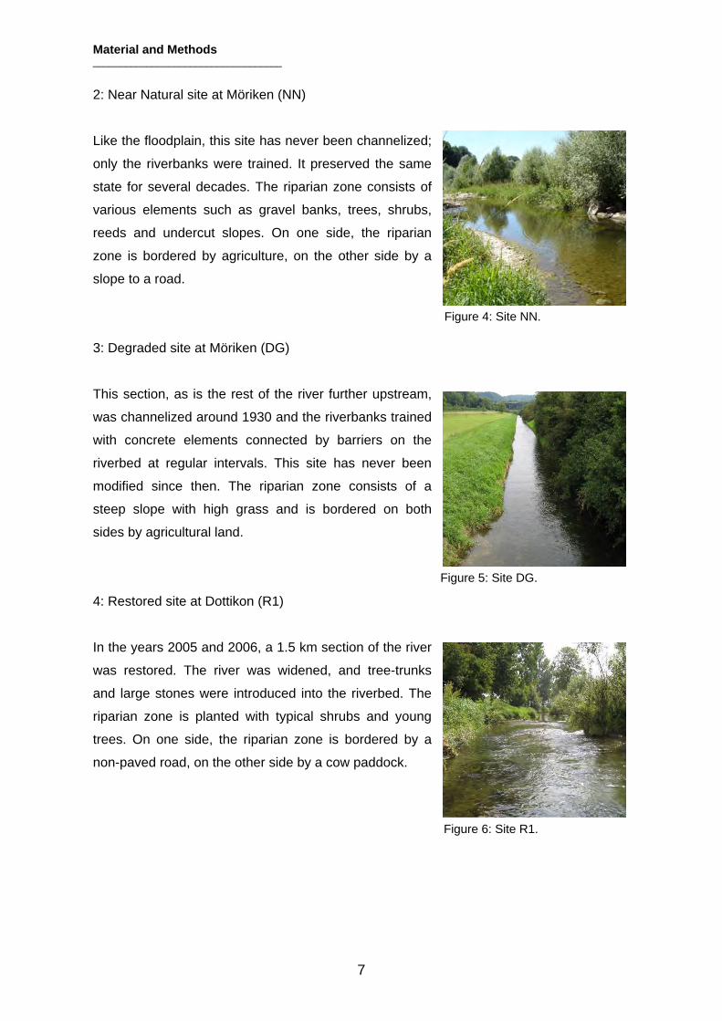
1: Floodplain at Möriken (FP)
This site has never been channelized; only the river
banks were trained. In 1999, a large flood removed the
training elements and the river broke its banks and
created a floodplain that is now protected as a floodplain
of national importance. The riparian zone consists mainly
of gravel banks with some shrubs and pioneer vegetation.
A part of it has undercut slopes where agricultural land
was removed. The riparian zone is bordered by
agriculture, forest and settlements.
Figure 3: Site FP.
Material and Methods ___________________________________
7
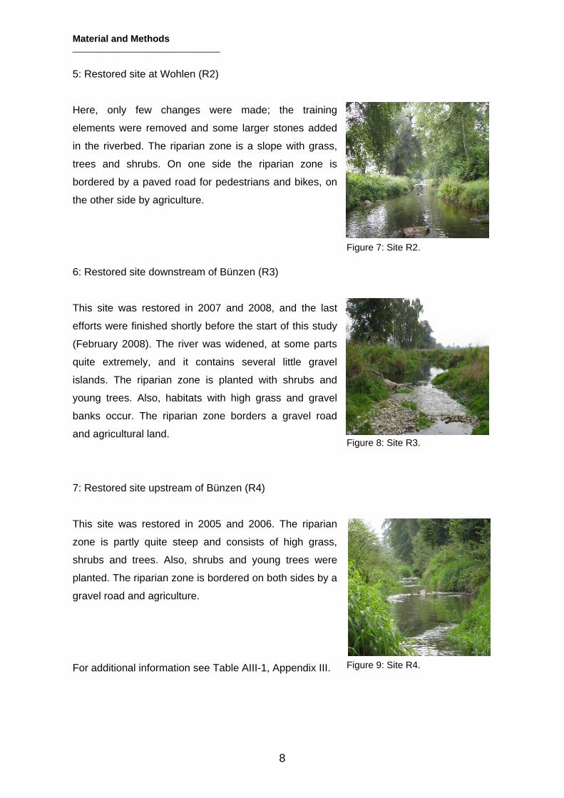
2: Near Natural site at Möriken (NN)
Like the floodplain, this site has never been channelized;
only the riverbanks were trained. It preserved the same
state for several decades. The riparian zone consists of
various elements such as gravel banks, trees, shrubs,
reeds and undercut slopes. On one side, the riparian
zone is bordered by agriculture, on the other side by a
slope to a road.
3: Degraded site at Möriken (DG)
This section, as is the rest of the river further upstream,
was channelized around 1930 and the riverbanks trained
with concrete elements connected by barriers on the
riverbed at regular intervals. This site has never been
modified since then. The riparian zone consists of a
steep slope with high grass and is bordered on both
sides by agricultural land.
4: Restored site at Dottikon (R1)
In the years 2005 and 2006, a 1.5 km section of the river
was restored. The river was widened, and tree-trunks
and large stones were introduced into the riverbed. The
riparian zone is planted with typical shrubs and young
trees. On one side, the riparian zone is bordered by a
non-paved road, on the other side by a cow paddock.
Figure 6: Site R1.
Figure 5: Site DG.
Figure 4: Site NN.
Material and Methods ___________________________________
8
5: Restored site at Wohlen (R2)
Here, only few changes were made; the training
elements were removed and some larger stones added
in the riverbed. The riparian zone is a slope with grass,
trees and shrubs. On one side the riparian zone is
bordered by a paved road for pedestrians and bikes, on
the other side by agriculture.
6: Restored site downstream of Bünzen (R3)
This site was restored in 2007 and 2008, and the last
efforts were finished shortly before the start of this study
(February 2008). The river was widened, at some parts
quite extremely, and it contains several little gravel
islands. The riparian zone is planted with shrubs and
young trees. Also, habitats with high grass and gravel
banks occur. The riparian zone borders a gravel road
and agricultural land.
7: Restored site upstream of Bünzen (R4)
This site was restored in 2005 and 2006. The riparian
zone is partly quite steep and consists of high grass,
shrubs and trees. Also, shrubs and young trees were
planted. The riparian zone is bordered on both sides by a
gravel road and agriculture.
For additional information see Table AIII-1, Appendix III.
Figure 7: Site R2.
Figure 8: Site R3.
Figure 9: Site R4.
Material and Methods ___________________________________
9
3.3 Morphological measurements
Three methods were applied to characterize the seven study sites:
3.3.1 Ecomorphology
The ecomorphological state of each site was determined according to the new “Methods
for the Investigation and Assessment of Running Waters in Switzerland (Modular Stepwise
Procedure)” (Buwal, 1998). This is a standard method in Switzerland and groups the sites
into four categories based on several morphological measurements.
I = natural / near-natural
II = little affected
III = highly affected
IV = non-natural / artificial
For sites NN, DG and R2, we had access to external data from the year 2001 (Source:
Peter Berner, Abteilung für Landschaft und Gewässer, Kanton Aargau). The remaining
sites were surveyed during summer 2008.
3.3.2 Indicators
Eleven Indicators that characterize river restoration success (Woosley et al., 2005) were
used to evaluate the study sites. They all give a value between 0 and 1, where 0
represents the artificial condition and 1 the natural condition.
Indicator 11, Fish habitats: Gives information about the availability of different refuges for
fish and their percentage of the whole water surface area.
Indicator 14, Variability in river width: Classifies into pronounced, limited or no variability in
river width.
Indicator 21, Abundance of riparian arthropods: Is based on carabid beetle abundance.
Indicator 35, Quality and grain size distribution of riverbed substrate: Gives information on
the percentage of the different grain size categories.
Material and Methods ___________________________________
10
Indicator 36, Structure of the riverbed: Percentage of different structures as riffles, pools,
etc. in the riverbed.
Indicator 37, Training of the riverbed: Estimates the percentage of river bed training and
characterizes the training structure.
Indicator 42, Width and composition of riparian zone: Includes the mean width of the
riparian zone and its composition, evaluating if it is appropriate for the river or artificial.
Indicator 44, Shoreline length: Compares the length of the shoreline to the length of the
corresponding river section.
Indicator 45, Structure of the riverbank: Estimates percentage of training elements and
number of different structures in areas without training elements.
Indicator 46, Training of the riverbank: Evaluates percentage and kind of training elements
3.3.3 Vegetation measurements
At each site, a sketch of the river and five meter width of each riverbank was drawn and all
vegetation structures (Table AIII-3, Appendix III) were plotted. Additionally, the percentage
of the total area of each vegetation structure was estimated. Four parameters to
characterize the vegetation were evaluated. First, vegetation diversity was determined by
counting the number of different vegetation structures occurring at each site. Secondly,
vegetation heterogeneity was determined as the number of alternating structures summed
up for both riversides. Furthermore, the Simpson-index and evenness for the vegetation
structures were calculated (Equations can be found in Appendix III).
Material and Methods ___________________________________
11
3.4 Biotic measurements
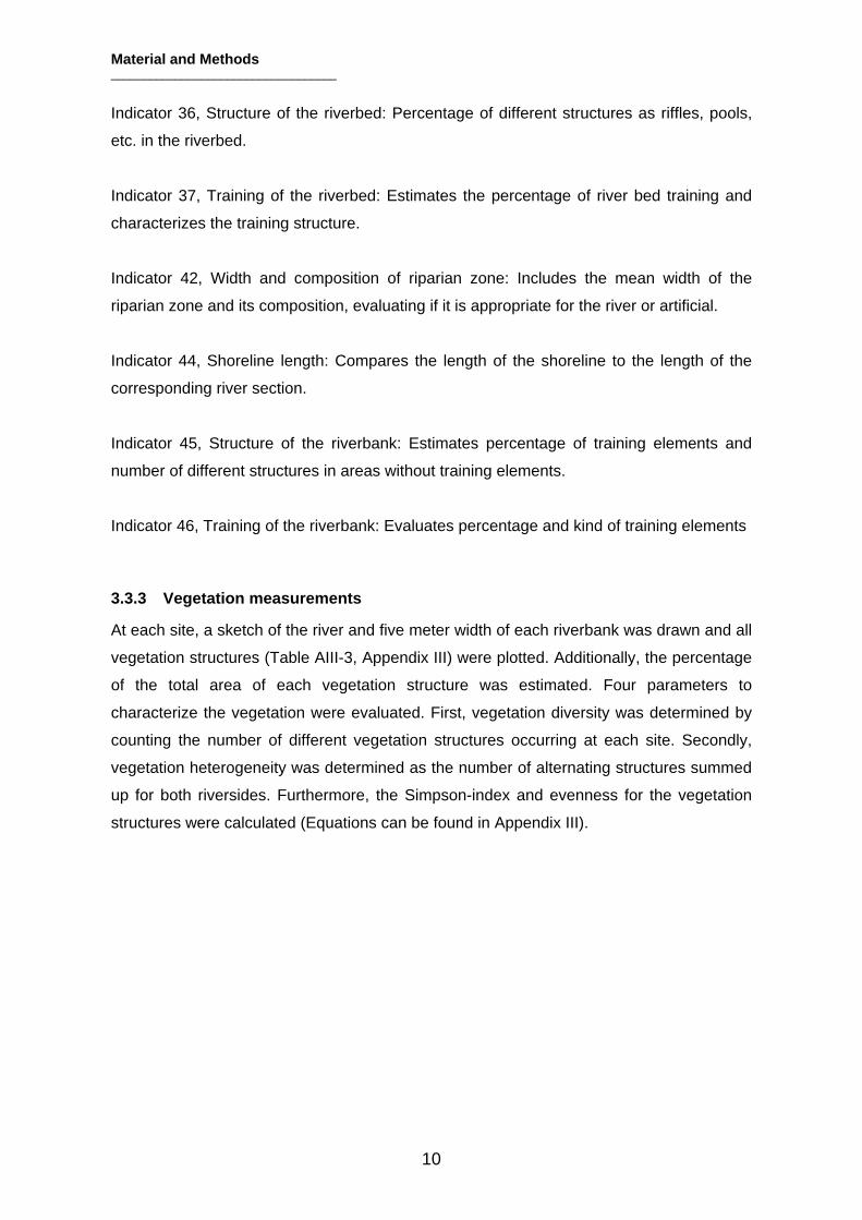
Three groups of arthropods were sampled:
1: Emerging aquatic Insects.
2: Terrestrial arthropod input into the river.
3: Riparian arthropod community.
Figure 10: Schematic overview of the sampling methods. The picture
shows the three sampled groups of invertebrates, their connection to the
river and the traps used to sample them . ET=emergence trap, DN=drift
net. FT=floating trap, PF=pitfall and HS=hand sampling
3.4.1 Sampling methods
To assess the biological diversity at each site, five different sampling methods were
applied.
Emergence traps (ET): Pyramidal emergence traps (for detailed description see Paetzold,
2004), with an opening of 0.25 m2 at the water surface, were placed on the river near the
shoreline (Figure 12A). Emerging insects were collected in an elector head filled with 70%
ethanol. On each sampling date, the traps were exposed for 24 hours.
Material and Methods ___________________________________
12
Drift nets (DN): Drift nets with a mesh of 400 μm and a rectangular opening of 15 x 20 cm
(Figure 12C) were exposed for 25 - 60 minutes. Flow velocity was measured at the mouth
of each net to calculate the volume of water filtered.
Floating traps (FT): A pan (0.25 m2) framed by styrofoam and containing water and one
drop of detergent (Glycerin) up to a filling height of ca 5 mm was fixed near the shoreline to
collect invertebrates falling into the water (Smock, 2006; Figure 12A). They were exposed
for 24 hours on each sampling date.
Pitfalls (PF): Plastic bins, 0.12 m high and with a quadrate opening of 9.5 x 9.5 cm were
dug into the ground near the shoreline (Figure 12C). They contained water with some
dishwashing liquid and were exposed for 24 hours on each sampling date.
Hand samplings (HS): With a self-made exhauster and forceps (Figure 12D), arthropods
were sampled in areas of 0.25 m2 near the shoreline. Vegetation and large stones were
partly removed.
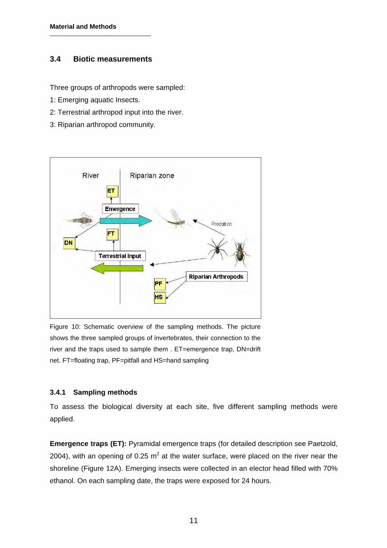
Four sampling surveys took place during the season (Figure 11 and Table AIII-2, Appendix
III) and for each trap method three samples were taken per site.
Figure 11: Discharge during sampling surveys. The values are from the measurement station in
Othmarsingen. The peak of maximum daily discharge during the May sampling is only relevant for
the lower three sites because it is caused by a flushing of the power plant Tieffurtmühle.
Material and Methods ___________________________________
13
A) B)
C) D)
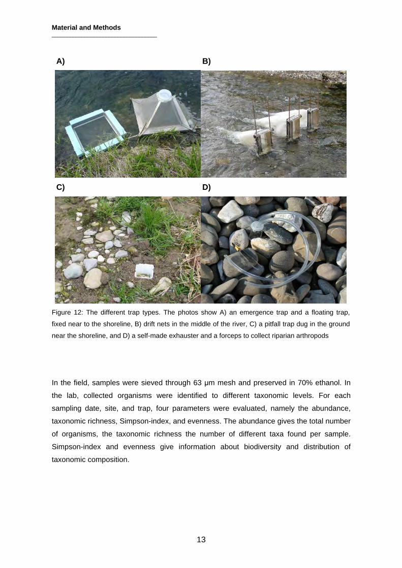
Figure 12: The different trap types. The photos show A) an emergence trap and a floating trap,
fixed near to the shoreline, B) drift nets in the middle of the river, C) a pitfall trap dug in the ground
near the shoreline, and D) a self-made exhauster and a forceps to collect riparian arthropods
In the field, samples were sieved through 63 μm mesh and preserved in 70% ethanol. In
the lab, collected organisms were identified to different taxonomic levels. For each
sampling date, site, and trap, four parameters were evaluated, namely the abundance,
taxonomic richness, Simpson-index, and evenness. The abundance gives the total number
of organisms, the taxonomic richness the number of different taxa found per sample.
Simpson-index and evenness give information about biodiversity and distribution of
taxonomic composition.
Material and Methods ___________________________________
14
3.5 Analysis of data
The parameters of the morphological measurements were analyzed using a Principal
Component Analysis (PCA) and the results presented in a scatter plot to evaluate
differences between the sites.
The influence of site and sampling date on the biotic parameters was tested by ANOVA
(linear model x ~ site * date) using the statistical program R (version 2.4). This analysis
was done for each trap type. To assure a normal distribution of the data, the values were
log transformed.
To determine relationships between the biotic and morphological parameters, a correlation
test was done using the program SPSS for each trap type.
To identify connections between insect emergence, riparian predators and terrestrial inputs,
a Pearson correlation test was done between the abundance of emerging insects from the
emergence traps and the abundance of spiders (all families), rove beetles (Staphilidae),
ground beetles (Carabidae) and riparian predators (the preceding three groups together)
from the pitfall traps and the terrestrial invertebrates in the floating traps.
Results ___________________________________
15
4 Results
4.1 Morphology
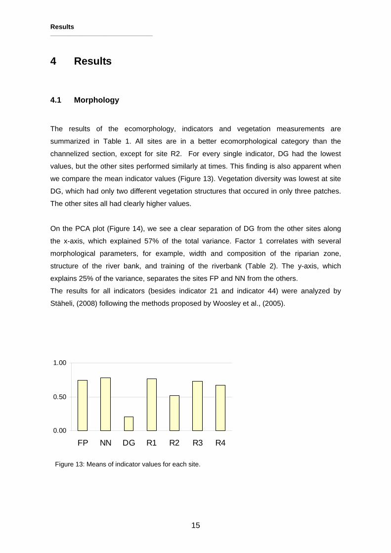
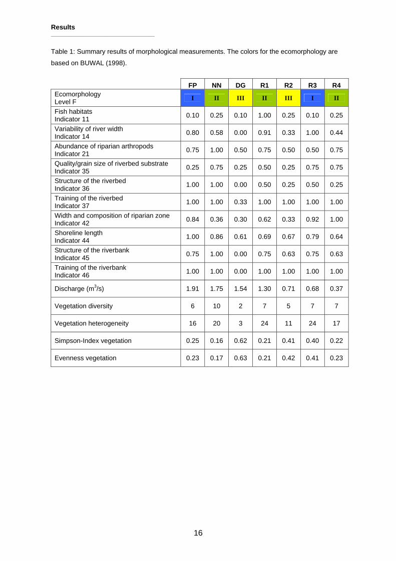
The results of the ecomorphology, indicators and vegetation measurements are
summarized in Table 1. All sites are in a better ecomorphological category than the
channelized section, except for site R2. For every single indicator, DG had the lowest
values, but the other sites performed similarly at times. This finding is also apparent when
we compare the mean indicator values (Figure 13). Vegetation diversity was lowest at site
DG, which had only two different vegetation structures that occured in only three patches.
The other sites all had clearly higher values.
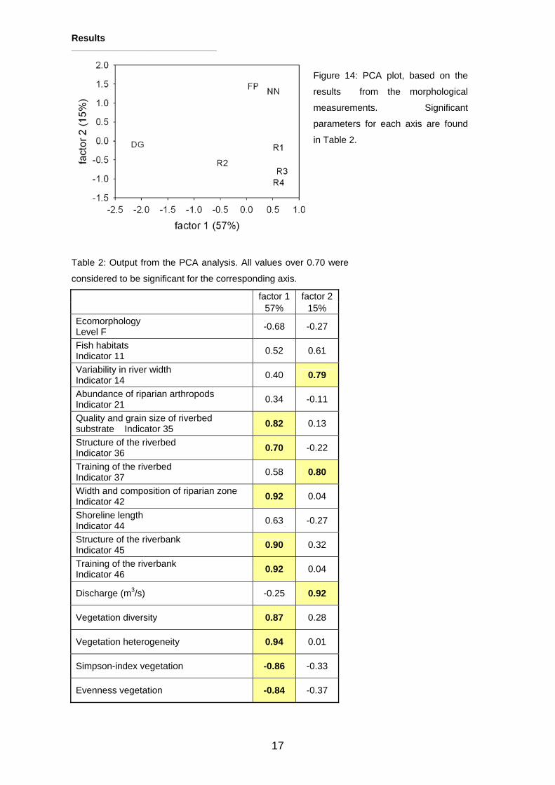
On the PCA plot (Figure 14), we see a clear separation of DG from the other sites along
the x-axis, which explained 57% of the total variance. Factor 1 correlates with several
morphological parameters, for example, width and composition of the riparian zone,
structure of the river bank, and training of the riverbank (Table 2). The y-axis, which
explains 25% of the variance, separates the sites FP and NN from the others.
The results for all indicators (besides indicator 21 and indicator 44) were analyzed by
Stäheli, (2008) following the methods proposed by Woosley et al., (2005).
Figure 13: Means of indicator values for each site.
0.00
0.50
1.00
FP NN DG R1 R2 R3 R4
Results ___________________________________
16
Table 1: Summary results of morphological measurements. The colors for the ecomorphology are
based on BUWAL (1998).
FP NN DG R1 R2 R3 R4 Ecomorphology Level F I II III II III I II
Fish habitats Indicator 11 0.10 0.25 0.10 1.00 0.25 0.10 0.25
Variability of river width Indicator 14 0.80 0.58 0.00 0.91 0.33 1.00 0.44
Abundance of riparian arthropods Indicator 21 0.75 1.00 0.50 0.75 0.50 0.50 0.75
Quality/grain size of riverbed substrate Indicator 35 0.25 0.75 0.25 0.50 0.25 0.75 0.75
Structure of the riverbed Indicator 36 1.00 1.00 0.00 0.50 0.25 0.50 0.25
Training of the riverbed Indicator 37 1.00 1.00 0.33 1.00 1.00 1.00 1.00
Width and composition of riparian zone Indicator 42 0.84 0.36 0.30 0.62 0.33 0.92 1.00
Shoreline length Indicator 44 1.00 0.86 0.61 0.69 0.67 0.79 0.64
Structure of the riverbank Indicator 45 0.75 1.00 0.00 0.75 0.63 0.75 0.63
Training of the riverbank Indicator 46 1.00 1.00 0.00 1.00 1.00 1.00 1.00
Discharge (m3/s) 1.91 1.75 1.54 1.30 0.71 0.68 0.37
Vegetation diversity 6 10 2 7 5 7 7
Vegetation heterogeneity 16 20 3 24 11 24 17
Simpson-Index vegetation 0.25 0.16 0.62 0.21 0.41 0.40 0.22
Evenness vegetation 0.23 0.17 0.63 0.21 0.42 0.41 0.23
Results ___________________________________
17
Table 2: Output from the PCA analysis. All values over 0.70 were
considered to be significant for the corresponding axis.
factor 1 factor 2 57% 15% Ecomorphology Level F -0.68 -0.27
Fish habitats Indicator 11 0.52 0.61
Variability in river width Indicator 14 0.40 0.79
Abundance of riparian arthropods Indicator 21 0.34 -0.11
Quality and grain size of riverbed substrate Indicator 35 0.82 0.13
Structure of the riverbed Indicator 36 0.70 -0.22
Training of the riverbed Indicator 37 0.58 0.80
Width and composition of riparian zone Indicator 42 0.92 0.04
Shoreline length Indicator 44 0.63 -0.27
Structure of the riverbank Indicator 45 0.90 0.32
Training of the riverbank Indicator 46 0.92 0.04
Discharge (m3/s) -0.25 0.92
Vegetation diversity 0.87 0.28
Vegetation heterogeneity 0.94 0.01
Simpson-index vegetation -0.86 -0.33
Evenness vegetation -0.84 -0.37
Figure 14: PCA plot, based on the
results from the morphological
measurements. Significant
parameters for each axis are found
in Table 2.
Results ___________________________________
18
4.2 Biotic assemblages
4.2.1 Abundance and diversity
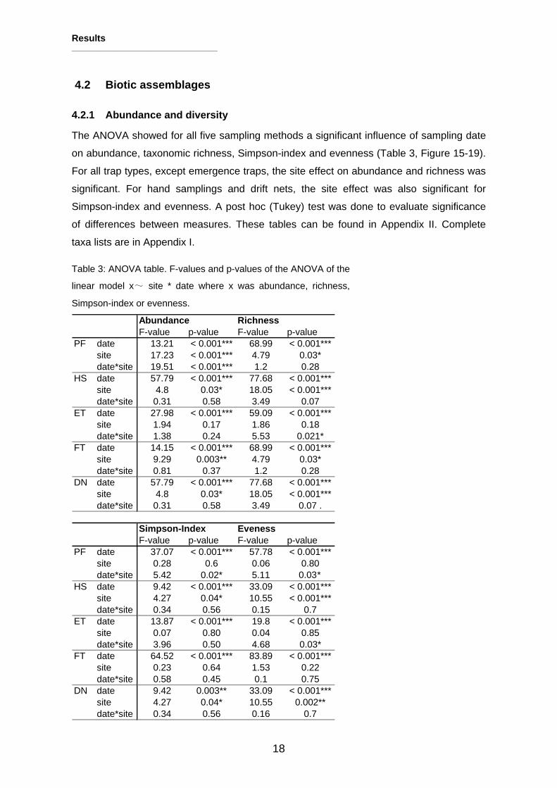
The ANOVA showed for all five sampling methods a significant influence of sampling date
on abundance, taxonomic richness, Simpson-index and evenness (Table 3, Figure 15-19).
For all trap types, except emergence traps, the site effect on abundance and richness was
significant. For hand samplings and drift nets, the site effect was also significant for
Simpson-index and evenness. A post hoc (Tukey) test was done to evaluate significance
of differences between measures. These tables can be found in Appendix II. Complete
taxa lists are in Appendix I.
Table 3: ANOVA table. F-values and p-values of the ANOVA of the
linear model x~ site * date where x was abundance, richness,
Simpson-index or evenness.
Abundance RichnessF-value p-value F-value p-value
PF date 13.21 < 0.001*** 68.99 < 0.001***site 17.23 < 0.001*** 4.79 0.03*date*site 19.51 < 0.001*** 1.2 0.28
HS date 57.79 < 0.001*** 77.68 < 0.001***site 4.8 0.03* 18.05 < 0.001***date*site 0.31 0.58 3.49 0.07
ET date 27.98 < 0.001*** 59.09 < 0.001***site 1.94 0.17 1.86 0.18date*site 1.38 0.24 5.53 0.021*
FT date 14.15 < 0.001*** 68.99 < 0.001***site 9.29 0.003** 4.79 0.03*date*site 0.81 0.37 1.2 0.28
DN date 57.79 < 0.001*** 77.68 < 0.001***site 4.8 0.03* 18.05 < 0.001***date*site 0.31 0.58 3.49 0.07 .
Simpson-Index EvenessF-value p-value F-value p-value
PF date 37.07 < 0.001*** 57.78 < 0.001***site 0.28 0.6 0.06 0.80date*site 5.42 0.02* 5.11 0.03*
HS date 9.42 < 0.001*** 33.09 < 0.001***site 4.27 0.04* 10.55 < 0.001***date*site 0.34 0.56 0.15 0.7
ET date 13.87 < 0.001*** 19.8 < 0.001***site 0.07 0.80 0.04 0.85date*site 3.96 0.50 4.68 0.03*
FT date 64.52 < 0.001*** 83.89 < 0.001***site 0.23 0.64 1.53 0.22date*site 0.58 0.45 0.1 0.75
DN date 9.42 0.003** 33.09 < 0.001***site 4.27 0.04* 10.55 0.002**date*site 0.34 0.56 0.16 0.7
Results ___________________________________
19
Emer
genc
e tr
ap: A
bund
ance
0
100
200
300
FPN
ND
GR
1R
2R
3R
4
# organisms / 0.25 m2
watersurface in 24h Emer
genc
e tr
ap: R
ichn
ess
05101520
FPN
ND
GR
1R
2R
3R
4
# taxa / 0.25 m2
watersurface in 24h
Emer
genc
e tr
ap: S
imps
on-In
dex
0
0.2
0.4
0.6
0.81
FPN
ND
GR
1R
2R
3R
4
Emer
genc
e tr
ap: E
venn
ess
0
0.2
0.4
0.6
0.81
FPN
ND
GR
1R
2R
3R
4
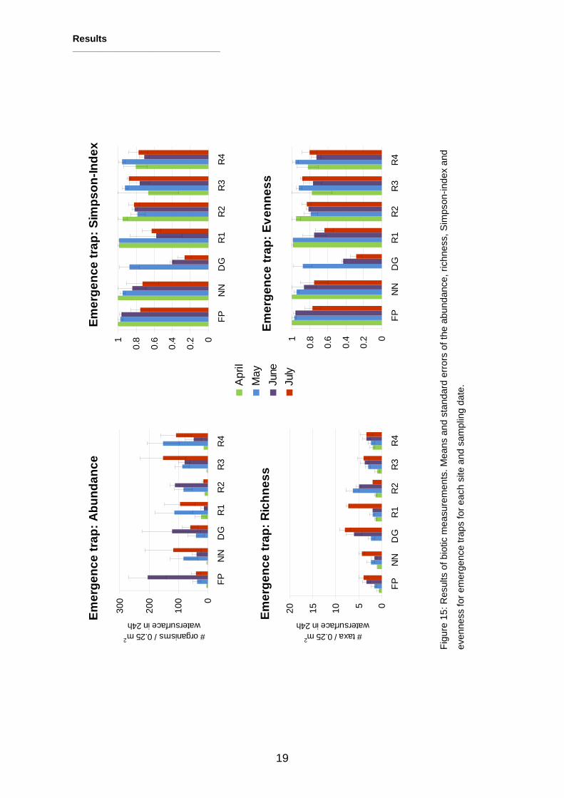
Figu
re 1
5: R
esul
ts o
f bio
tic m
easu
rem
ents
. Mea
ns a
nd s
tand
ard
erro
rs o
f the
abu
ndan
ce, r
ichn
ess,
Sim
pson
-inde
x an
d
even
ness
for e
mer
genc
e tra
ps fo
r eac
h si
te a
nd s
ampl
ing
date
. Apr
ilM
ayJu
neJu
ly
Results ___________________________________
20
Drif
t net
: Abu
ndan
ce
050100
150
200
250
FPN
ND
GR
1R
2R
3R
4
# organisms / m3 water
Drif
t net
: Ric
hnes
s
05101520
FPN
ND
GR
1R
2R
3R
4
# taxa / m3 water
Drif
t net
: Sim
pson
-Inde
x
0
0.2
0.4
0.6
0.81
FPN
ND
GR
1R
2R
3R
4
Drif
t net
: Eve
nnes
s
0
0.2
0.4
0.6
0.81
FPN
ND
GR
1R
2R
3R
4
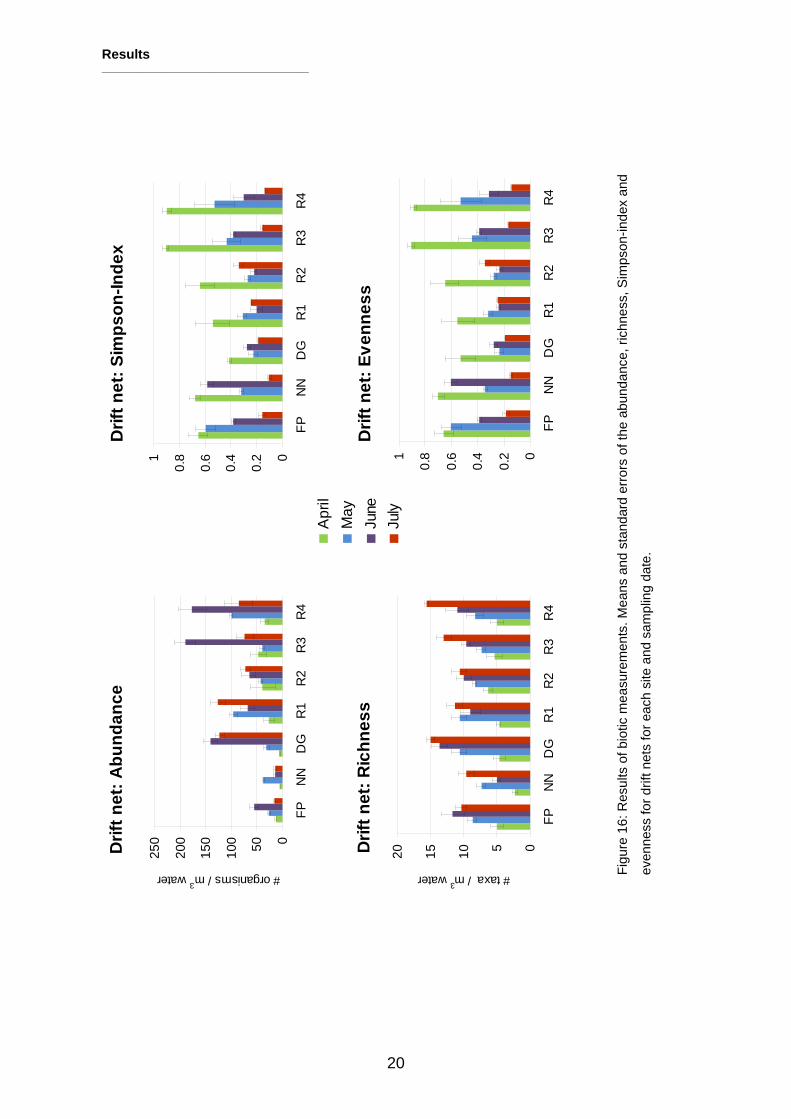
Figu
re 1
6: R
esul
ts o
f bio
tic m
easu
rem
ents
. Mea
ns a
nd s
tand
ard
erro
rs o
f the
abu
ndan
ce, r
ichn
ess,
Sim
pson
-inde
x an
d
even
ness
for d
rift n
ets
for e
ach
site
and
sam
plin
g da
te.
Apr
ilM
ayJu
neJu
ly

Results ___________________________________
21
Figu
re 1
7: R
esul
ts o
f bio
tic m
easu
rem
ents
. Mea
ns a
nd s
tand
ard
erro
rs o
f the
abu
ndan
ce, r
ichn
ess,
Sim
pson
-inde
x an
d
even
ness
for f
loat
ing
traps
for e
ach
site
and
sam
plin
g da
te.
Floa
ting
trap
: Abu
ndan
ce
020406080
FPN
ND
GR
1R
2R
3R
4
# organisms / 0.25 m2 in 24h
Floa
ting
trap
: Ric
hnes
s
05101520
FPN
ND
GR
1R
2R
3R
4
# taxa / 0.25 m2 in 24h
Floa
ting
trap
: Sim
pson
-Inde
x
0
0.2
0.4
0.6
0.81
FPN
ND
GR
1R
2R
3R
4
Floa
ting
trap
: Eve
nnes
s
0
0.2
0.4
0.6
0.81
FPN
ND
GR
1R
2R
3R
4
Apr
ilM
ayJu
neJu
ly
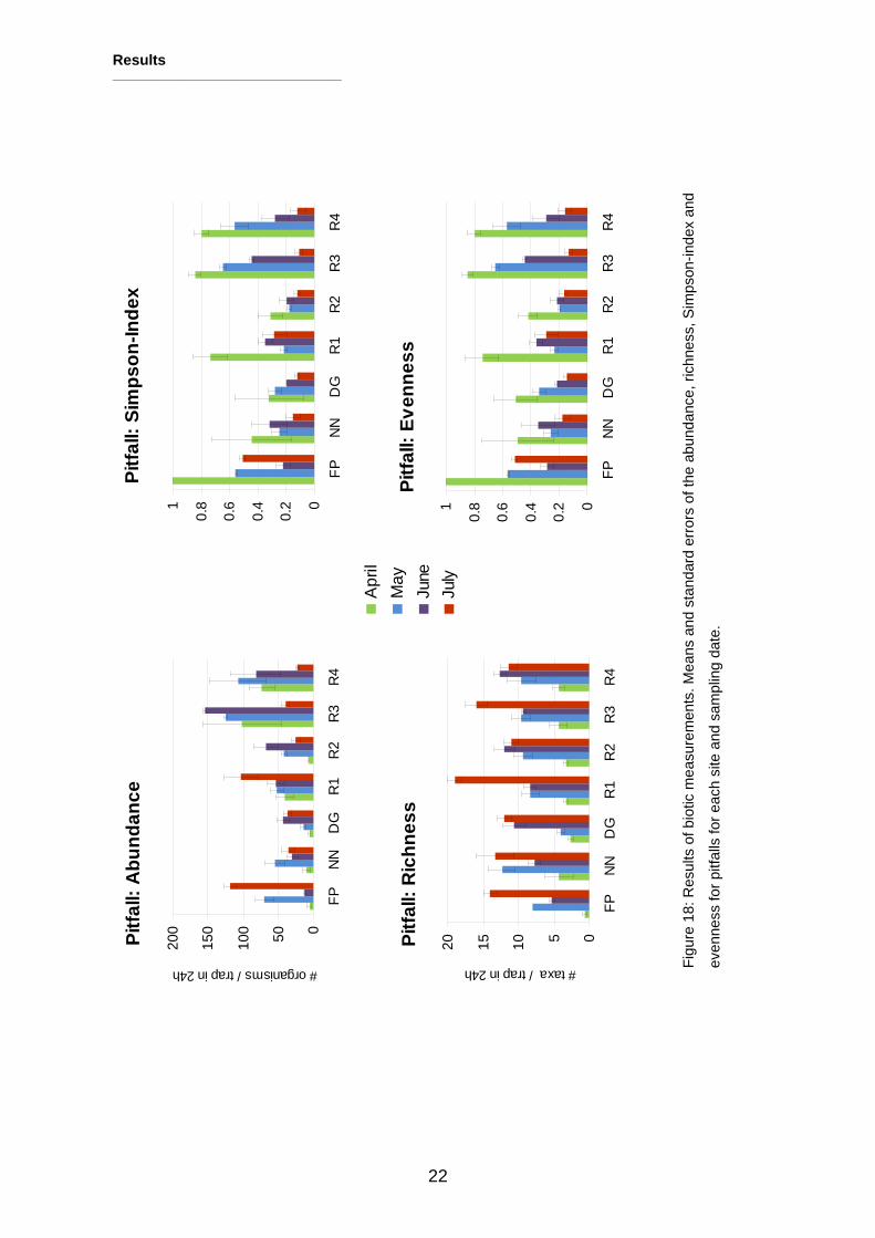
Results ___________________________________
22
Figu
re 1
8: R
esul
ts o
f bio
tic m
easu
rem
ents
. Mea
ns a
nd s
tand
ard
erro
rs o
f the
abu
ndan
ce, r
ichn
ess,
Sim
pson
-inde
x an
d
even
ness
for p
itfal
ls fo
r eac
h si
te a
nd s
ampl
ing
date
.
Pitfa
ll: A
bund
ance
050100
150
200
FPN
ND
GR
1R
2R
3R
4
# organisms / trap in 24h
Pitfa
ll: R
ichn
ess
05101520
FPN
ND
GR
1R
2R
3R
4
# taxa / trap in 24h
Pitfa
ll: S
imps
on-In
dex
0
0.2
0.4
0.6
0.81
FPN
ND
GR
1R
2R
3R
4
Pitfa
ll: E
venn
ess
0
0.2
0.4
0.6
0.81
FPN
ND
GR
1R
2R
3R
4
Apr
ilM
ayJu
neJu
ly
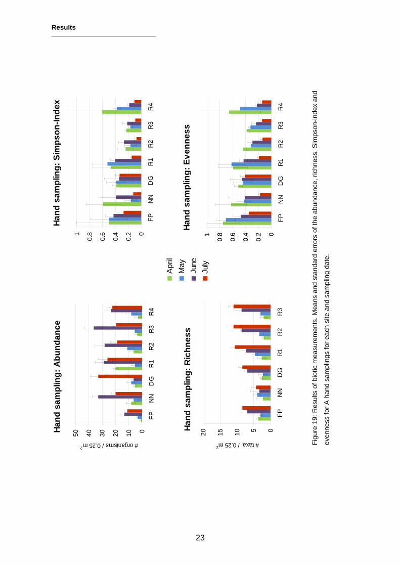
Results ___________________________________
23
Figu
re 1
9: R
esul
ts o
f bio
tic m
easu
rem
ents
. Mea
ns a
nd s
tand
ard
erro
rs o
f the
abu
ndan
ce, r
ichn
ess,
Sim
pson
-inde
x an
d
even
ness
for A
han
d sa
mpl
ings
for e
ach
site
and
sam
plin
g da
te.
Hand
sam
plin
g: A
bund
ance
01020304050
FPN
ND
GR
1R
2R
3R
4
# organisms / 0.25 m2
Hand
sam
plin
g: R
ichn
ess
05101520
FPN
ND
GR
1R
2R
3
# taxa / 0.25 m2
Hand
sam
plin
g: S
imps
on-In
dex
0
0.2
0.4
0.6
0.81
FPN
ND
GR
1R
2R
3R
4
Hand
sam
plin
g: E
venn
ess
0
0.2
0.4
0.6
0.81
FPN
ND
GR
1R
2R
3R
4
Apr
ilM
ayJu
neJu
ly
Results ___________________________________
24
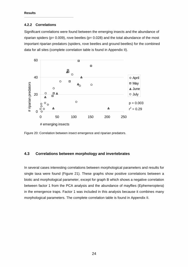
4.2.2 Correlations
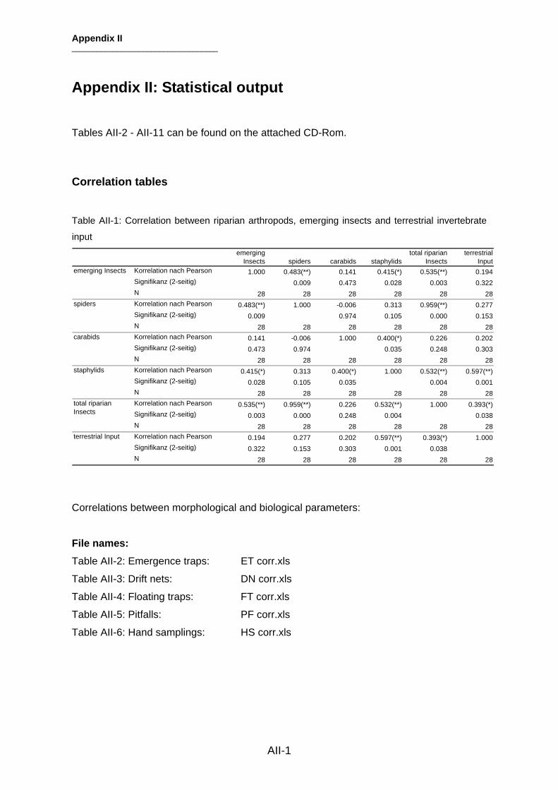
Significant correlations were found between the emerging insects and the abundance of
riparian spiders (p= 0.009), rove beetles (p= 0.028) and the total abundance of the most
important riparian predators (spiders, rove beetles and ground beetles) for the combined
data for all sites (complete correlation table is found in Appendix II).
0
20
40
60
0 50 100 150 200 250
# emerging insects
# rip
aria
n pr
edat
ors
AprilMayJuneJuly
Figure 20: Correlation between insect emergence and riparian predators.
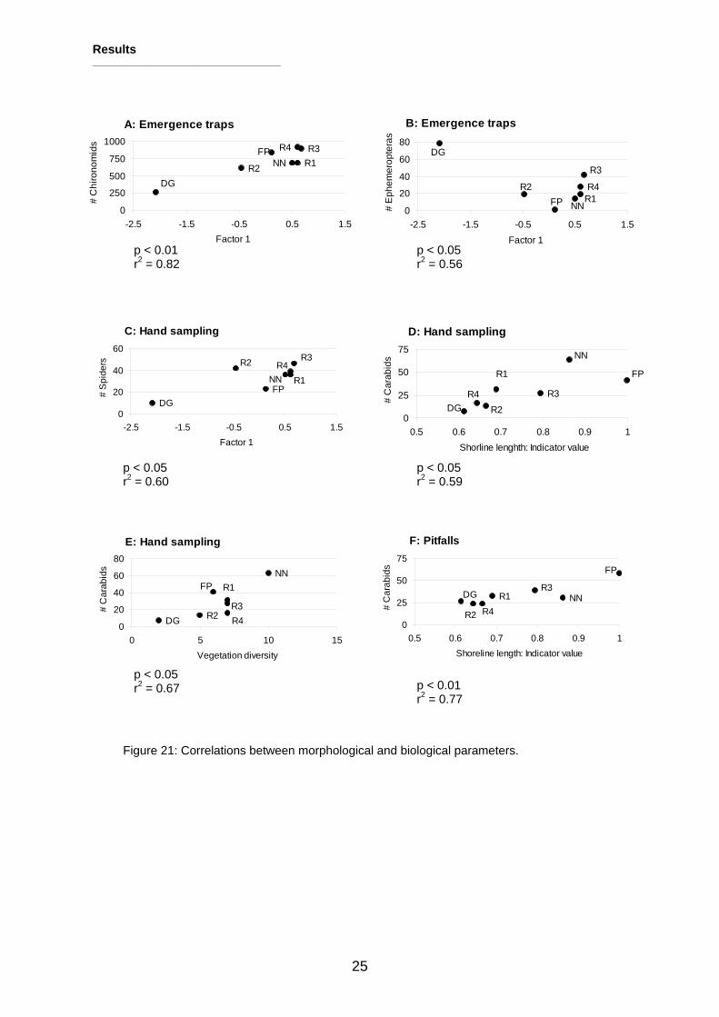
4.3 Correlations between morphology and invertebrates
In several cases interesting correlations between morphological parameters and results for
single taxa were found (Figure 21). These graphs show positive correlations between a
biotic and morphological parameter, except for graph B which shows a negative correlation
between factor 1 from the PCA analysis and the abundance of mayflies (Ephemeroptera)
in the emergence traps. Factor 1 was included in this analysis because it combines many
morphological parameters. The complete correlation table is found in Appendix II.
p = 0.003
r2 = 0.29
Results ___________________________________
25
A: Emergence traps
FPNN
DG
R1R2
R3R4
0
250
500
750
1000
-2.5 -1.5 -0.5 0.5 1.5Factor 1
# C
hiro
nom
ids
B: Emergence traps
FP NN
DG
R1R2
R3
R4
0
20
40
60
80
-2.5 -1.5 -0.5 0.5 1.5Factor 1
# E
phem
erop
tera
s
C: Hand sampling
R4R3R2
R1
DG
NNFP
0
20
40
60
-2.5 -1.5 -0.5 0.5 1.5Factor 1
# S
pide
rs
D: Hand sampling
FP
NN
DG
R1
R2
R3R4
0
25
50
75
0.5 0.6 0.7 0.8 0.9 1Shorline lenghth: Indicator value
# C
arab
ids
E: Hand sampling
FPNN
DG
R1
R2R3R40
20
40
60
80
0 5 10 15Vegetation diversity
# C
arab
ids
F: Pitfalls
FP
NNR4
R1
R2
R3DG
0
25
50
75
0.5 0.6 0.7 0.8 0.9 1Shoreline length: Indicator value
# C
arab
ids
p < 0.05 r2 = 0.67
p < 0.05 r2 = 0.60
p < 0.01 r2 = 0.82
p < 0.05 r2 = 0.56
p < 0.05 r2 = 0.59
p < 0.01 r2 = 0.77
Figure 21: Correlations between morphological and biological parameters.
Discussion ___________________________________
26
5 Discussion
5.1 Morphology
A historical or a natural reference site is missing in the Bünz; therefore, no statements can
be made about how near the restored sites are now to their former natural state. But this
was not really the goal of the restorations because the achievement to a natural state is
not possible under todays conditions in this intensely farmed and densely inhabited Swiss
midland (Woosley et al., 2005). The situation at the channelized site DG can be
considered the worst state of the river except where it flows inside towns and if it is entirely
within a culvert. All the restored sites (R1 to R4) were once in a state very near to this
situation at DG. Therefore, it seems reasonable to compare the restored site to the
degraded site and assess a positive divergence of the morphological values from these
evaluated for site DG as an improvement. Stäheli (2008), who worked with the same data,
analyzed the data by using site DG as a degraded reference. This approach is adequate if
natural references are missing and the degraded state is of interest to evaluate
deficiencies of a system (Rohde, 2004). Stäheli (2008) could show that all sites performed
better compared to the degraded reference. The best site was FP, which is a special case
compared to the rest because the morphological state here is caused by a natural event; it
can be called a “restoration by nature”. Here the river also has the possibility to change its
course, which allows a certain dynamic that is characteristic of natural river corridors
(Ward et al., 2002). The relatively low ranking of NN in this analysis can be explained by
the fact that the width of the riparian zone, which is an important quality measurement, is
quite low at this site. It is evaluated regarding the width of the river itself, which is much
wider at NN than in the more upstream restored sites and requires, therefore, an
accordingly wider riparian zone. A wide riparian area is not possible because of the land
tenure of the neighboring area, which is used as agricultural land.
In this study, several additional morphological measurements were used from those in
Stäheli (2008). First, two indicators were included in the analysis that give information
about the riparian zone, namely shoreline length (Indicator 44) and the density of riparian
arthropods (Indicator 21). Shoreline length reflects the morphological complexity of a river
section that is characteristic for a natural river system (Woosley et al., 2006). This indicator
showed quite high values at sites NN and R3. These two sites meander more than the
Discussion ___________________________________
27
other sites and contain one or several little islands. For Indicator 21, the maximum could
be reached at NN, while the lowest values were found at DG, R2 and R3. The reason for
this result may be the low habitat heterogeneity and steep riparian zone at DG and R2. At
site R3, the time factor may play an important role as restoration at this site was finished
some months before this study. Further aspects of correlations between morphology and
riparian arthropods are discussed in paragraph 5.3.2.
Secondly, the riparian vegetation was investigated. Here, we clearly see one of the main
deficiencies of the channelized section. Only two vegetation structures were found, and on
one river side only one structure is present (Figure 5). Habitat heterogeneity of the riparian
zone that is crucial for biodiversity (Ward, 1998) is therefore very low. Here again, the
natural site (NN) performs well. One reason may be the long time period of no change that
allowed the development of diverse vegetation. This leads to the assumption that restored
sites that are relatively young can reach their full potential only after some years.
In conclusion, it can be said that all sites are in a better ecomorphological state than the
channelized section (DG). The PCA-plot (Figure 13) shows a clear separation of site DG
from the other sites along factor 1. Factor 1 is highly correlated with several parameters
such as, e.g., vegetation diversity (Table 2). Site R2 was placed between DG and the
others. At this site, little restoration effort was made, and only the training elements were
removed. Regardless, a positive effect is still apparent. As the riparian zone is quite narrow
and steep at this site, the rehabilitation potential is low, and the river had little chance to
expand. Based on the good performance of the floodplain (FP), which was actually
restored naturally, it can be assumed that the removal of lateral training elements and
additional availability of space for the river to expand can allow good restoration success at
low efforts and costs.
Hypothesis I: The ecomorphological state will differ between the different sites. Sites
affected by human activities will be in a worse morphological state than natural or restored
sites.
This hypothesis can be accepted because morphological differences between sites are
apparent. It could be showed that site DG, which was heavily affected by humans, is in the
worst morphological state of all the sites.
Discussion ___________________________________
28
5.2 Biotic assemblages
5.2.1 Abundance and diversity
Data analysis was done for each trap separately because of the different sampling
approaches. For all traps, the biotic assemblages showed significant differences between
the different sampling dates. This corresponded to initial expectations based on the
knowledge of seasonal changes in biotic community structure at one place. Thus, it is
important to collect several dates to cover the entire taxonomic phenology (e.g. Dineen et
al., 2007).
Samples from the emergence traps showed no site effect, and only seasonal changes
were apparent. No clear trend or seasonal peak was obvious. The main taxa in the
samples were dipterans, the most frequent family the chironomids. Similar results by
sampling emerging aquatic insects were found by Judd (1962).
The drift net samples showed large seasonal differences, but no clear seasonal peak was
apparent. A reason could be that the sampling was not always done at the same time of
day. The 24 hour drift net survey (Appendix III) showed large diurnal changes and in
addition, the single data surveys spanned about one week and the weather conditions
sometimes changed. Site effects were most pronounced in summer (June and July); for
example, R3 and R4 showed significantly the greatest abundance in June. There were no
sites that showed a clear greater or lower abundance in drift. It is possible that other
factors may have produced these effects.
Regarding the results of the floating traps, two findings are interesting. Firstly, sites FP
and DG were the only ones that showed no seasonal changes. Secondly, site R2 had
always the highest abundance of terrestrial inputs; in June it differed significantly from all
the other sites except for site R3. Sites FP and DG had the lowest canopy coverage, site
R2 the highest. For terrestrial inputs, the vegetation type, coverage and succession state
were important, and the terrestrial input changed with the seasonal change in vegetation
(Wipfli, 1997). Thus, if almost no vegetation exists that can provide invertebrate input, no
changes in input abundance or composition can be expected. This confirms the
importance of canopy for the abundance of terrestrial invertebrate input.
Site effects in the pitfall and hand sampling samples were only small, but if present
mostly pronounced in summer. In June, site R3 had significantly the greatest abundance,
Discussion ___________________________________
29
and in July the sites FP and R1 had the greatest abundance. In the hand samples, the
evenness at site DG was in July significantly higher than at all other sites except for FP ,
which differed from no other sites. To conclude, it can be said that in cases where site
effects were apparent, restored sites either had significantly greater abundance or diversity
or the degraded site had significantly lower abundance and diversity.
Hypothesis II: Differences between sites and season will be apparent in the terrestrial and
aquatic adult invertebrate assemblages.
Hypothesis II can partly be accepted. Seasonal differences differed between sites and trap
types, but generally the abundance and richness were higher in summer and, therefore,
Simpson-index and evenness were lower. Site effects were apparent, but not in all trap
types and they did not allow a clear ranking of the sites.
5.2.2 Correlations between aquatic and terrestrial communities
The existing correlation of riparian arthropods and aquatic insect emergence indicates a
trophic connection of the riparian zone and the river because emerging insects are an
energy source for riparian predators (e.g. Burdon and Harding, 2008). The terrestrial input
was not correlated with these values. A reason for that could be that, on one side, the
abundance of terrestrial input is highly influenced by the riparian vegetation (Wipfli, 1997)
and, on the other side, the terrestrial input does not directly influence the aquatic insect
population. It serves mainly as an important food source for fish (Allan et al., 2003).
Hypothesis III: There will be a relationship between the emergence of aquatic insects,
riparian predators, and input of terrestrial invertebrates into the river at the different sites.
The third hypothesis can not completely be accepted because the terrestrial input does not
correlate with the other factors.
Discussion ___________________________________
30
5.3 Correlations between morphology and biology
5.3.1 Aquatic communities
In emergence traps, two significant correlations were notable. Firstly, the abundance of
chironomids, which was the main taxon, in all emergence traps correlated significantly (p <
0.05) and positively with factor 1 from the PCA analysis that combines several
morphological factors (Table 2). Additionally, chironomid abundance correlated with the
indicators for training of the riverbank and riverbed (both p < 0.05). This indicates an
enhanced emergence at sites with better morphological condition and fewer training
structures on the riverbed or on the riverbank.
Secondly, factor 1 is significantly (p < 0.05) negatively correlated with the abundance of
mayflies. The high abundance at site DG is especially notable. Here, the abundance is
more than twice as high as at the other sites. This result is surprising because the data for
macrozoobenthos (Stäheli, 2008) showed little difference between the sites in the
abundance of mayflies. Two explanations are possible. First, there is the possibility that
the mayfly larvae drift and then emerge at this particular site due to reasons that were not
addressed in this study. The alternative explanation is that the type of emergence trap is
not appropriate for this special case. When possible, traps were placed in a slow flowing
part of each site. At DG, no such habitats were available and the flow velocity under the
emergence traps was quite high. This kind of trap is usually not considered for fast flowing
streams. It is also possible that adult aquatic insects use the trap as an ovipositioning
place and end up in the elector head of the trap. This was showed by a study of Mundie,
(1956) for the mayfly family Baetidae, which was actually the most abundant taxa in the
emergence trap samples for this site.
Discussion ___________________________________
31
5.3.2 Terrestrial communities
Carabid beetles and spiders are both characteristic species of river banks (Kunz, 2006).
The apparent correlations of carabid beetles with the indicator for shoreline length and
vegetation diversity, both reflect heterogeneity, as well as the correlation of spider
abundance with factor 1 from the PCA analysis indicates that riparian arthropods are
influenced by morphological factors and occur in higher abundance in morphologically
intact or restored sites. This is supported by a study of Bosccaini et al., (2000) who
showed that carabids are sensitive to environmental change and channelization. The
shoreline length reflects the morphological complexity of a river section (Woosley et al.,
2006). Complex and heterogeneous habitats influence the abundance of riparian
arthropods. Thus ameliorations in morphology can have a positive influence on riparian
arthtopods.
Hypothesis IV: Measured biotic parameters will correlate with the morphological
characteristics of the different sites.
This hypothesis can be accepted because of above mentioned significant correlations.
Discussion ___________________________________
32
5.4 Conclusions
Restoration clearly influenced the morphological state of the various sites in a positive way.
The Bünz could be potential habitat for many organisms such as invertebrates and fish.
Also, the floodplain site that was restored naturally and site R2 where only little restoration
efforts were made, showed a positive change compared to the channelized site. Allowing
the river to expand by removing lateral training elements and providing space may be a
good approach as a supplement to usual restoration efforts and may help reduce costs.
A better morphological state or a greater availability of habitats does not instinctively lead
to a more abundant or more diverse biotic assemblage. The physical structures alone do
not bring back organisms into the system (Field of Dreams Approach, Hildebrand et al.,
2005). In planning restorations, morphological and ecological processes should be
considered (e.g. Kondolf, 1998). The connectivity with habitats where the target species
pool is present is crucial for the recolonisation of restored habitats.
The recolonisation potential of the Bünz valley was never considered and may be a
restriction. This may be a reason for the poorly pronounced site effects in biotic
assemblages. Another reason could be that the restored sites are quite young and the
biotic community could not yet use the full potential of existing ecological niches.
The correlations of some biotic parameters with measured morphological parameters
suggest that an improvement in morphology can have positive effects on terrestrial and
aquatic invertebrate assemblages.
The restoration efforts at the Bünz showed some positive effects on biotic assemblages
and further restorations that connect the morphologically good habitats may move the
system to a better ecological state. However it is not excluded that some restrictions exist
that impede the river to come to its full potential.

Acknowledgements ___________________________________
33
6 Acknowledgements Thanks to...
...Chris Robinson for supervising my thesis, helping with statistics, reviewing the text and
correcting my English as well as for supplying me with healthy fruits.
...Klement Tockner for being my second examiner.
...Tino Stäheli for good collaboration, field work assistance and entertainment during long
hours sitting in front of the binocular and identifying insects.
...Maria Alp for reviewing my thesis and giving me much helpful advice.
...Caroline Baumgartner for the good time we had being desk-neighbors and for helping
me out with many language and other problems.
...the whole ECO-Department for the good working atmosphere, lots of nice chats in my
coffee-room-office and funny hours at Friday beers and barbecues.
...Peter Moser for many hours of field work assistance and for his mental support during
my master thesis.
...,last but not least, my parents Rosmarie and Franz Baumgartner who enabled my
education and who always supported me.
References ___________________________________
34
7 References
Allan, J. D., M.S. Wipfli, J.P. Caouette, A. Prussian and J. Rodgers. 2003. Influence of
streamside vegetation on inputs of terrestrial invertebrates to salmonid food webs.
Canadian Journal of Fisheries and Aquatic Sciences.Vol. 60, Issue 3. 309-320
Baxter, C.V., K.D. Fausch and W.C. Saunders. 2005. Tangled webs: reciprocal flows of
invertebrate prey link streams and riparian zones. Freshwater Biology Vol.50. 201-220.
Boscaini, A., A. Franceschini and B. Maiolini. 2000. River ecotones: carabid beetles as a
tool for quality assessment. Hydrobiologia 422/423. 173-181.
Burdon, F.J. and J.S. Harding. 2008. The linkage between riparian predators and aquatic
insects across a stream-resource spectrum. Freshwater Biology Vol. 53. 330-346.
Burger, S. 2007. Bünz: Vom Kanal zum dynamischen Bach. Umwelt Aargau Nr. 37. 9-16.
Buwal (Bundesamt für Umwelt, Wald und Landschaft). 1998. Methoden zur Untersuchung
und Beurteilung der Fliessgewässer in der Schweiz. Ökomorphologie Stufe F
(flächendeckend). Mitteilungen zum Gewässerschutz Nr. 27.
Chinery, M. 2004. Parey’s Buch der Insekten. 326 pp.
Dineen, G., S.S.C. Harrison and P.S. Giller. 2007. Seasonal analysis of aquatic and
terrestrial invertebrate supply to streams with grassland and deciduous riparian
vegetation. Biology & Environment: Proceedings of the Royal Irish Academy, Vol. 107B,
No.3. 167-182.
Hering, D. and H. Plachter. 1997. Riparian ground beetles (Coleoptera, Carabidae) preying
on aquatic invertebrates: a feeding strategy in alpine floodplains. Oecologia 111. 261-
270.
Hildebrand, R.H., A.C. Watts and A.M. Randle. 2005. The myths of restoration ecology.
Ecology and Society, Vol. 10(1). 19. http://www.ecologyandsociety.org/vol10/iss1/art19
References ___________________________________
35
Iwata, T. 2007. Linking stream habitats and spider distribution: spatial variations in trophic
transfer across a forest-stream boundary. Ecological Research, Vol. 22, Issue 4. 619-
628
Judd, W.W. 1962. A study of the population of Insects emerging as adults from Medway
creek at Arva, Ontario. American Midland Naturalist, Vol. 68, No.2. 463-473.
Kondolf, D.M. 1998. Lessons learned from river restoration projects in California. Aquatic
Conservation: Marine and Freshwater Ecosystems. Vol. 8. 39-52.
Kunz, Y. 2006. Terrestrische Indikatoren zur Fliessgewässerbeurteilung? Habitatsdiversität,
aArthropoden und Uferlängen an Flüssen unterschiedlicher hydrologischer und
morphologischer Beeinträchtigungen. Diploma Thesis Eawag Dübendorf and ETH
Zürich. 76 pp.
Lake, P.S., N. Bond and P. Reich. 2007. Linking ecological theory with stream restoration.
Freshwater Biology 52. 597-615
Marczak, L.B and J.S. Richardson. 2007. Spiders and subsidies: Results from the riparian
zone of a costal temperate rainforest. Journal of Animal Ecology, Vol. 76. 687-694.
Mundie, J.H. 1956. Emergence traps for aquatic insects. Internationale Vereinigung für
theoretische und angewandte Limnologie: Mitteilungen. No. 7. 13 pp.
Naiman, R.J., H. Decamps and M Pollock. 1993. The role of riparian corridors in
maintaining regional biodiversity. Ecological Applications, Vol.3, No. 2. 209-212.
Paetzold, A. 2004. Life at the Edge- Aquatic-terrestrial interactions along rivers.
Dissertation ETH No. 15825.
Paetzold, A, C.J. Schubert and K. Tockner. 2005. Aquatic terrestrial linkages along a
braided-river: Riparian arthropods feeding on aquatic insects. Ecosystems Vol. 8. 748-
759.
Palmer, M.A., E.S. Bernhardt, J.D. Allan, P.S. Lake, G.Alexander, S.Brooks, J. Carr, S.
Clayton, C.N. Dahm, J. Follstad Sha, D.L. Galat, S.G. Loss, P. Goodwin, D.D. Hart,
B.Hassett, R.Jenkinson, G.M. Kondolf, R. Lave, J.L. Meyer, T.K. O’Donnel, L.Pagano

References ___________________________________
36
and E. Sudduth. 2005. Standards for ecologically succesfull river restoration. Journal of
Applied Ecology 42. 208-217.
Rohde, S. 2004. River Restoration: Potential and limitations to re-establish riparian
landscapes. Assessment & Planning. Dissertation ETH No. 15496.
Smock, L.A. 2005. Macroinvertebrate Dispersal. Methods in stream ecology. Edited by F.R.
Hauer and G.A. Lamberti. Second Edition. Chapter 21, 465-487.
Stäheli, T. 2008. Revitalisierungen entlang der Bünz: Zusammenhänge zwischen
Hydromorphologie und Makrozoobenthos. Diplomarbeit, Eawag und ETH Zürich.
Stresemann, E, H.J. Hannemann, B. Klausnitzer and K. Senglaub. 2000. Exkursionsfauna
von Deutschland, Band 2: Wirbellose: Insekten. Spektrum Akademischer Verlag.
Ward, J.V. 1998. Riverine landscapes: Biodiversity patterns, disturbance regimes, and
aquatic conservation. Biological Conservation Vol. 83, No. 3. 269-278.
Ward, J.V., K. Tockner, D.B. Arscott and C. Claret. 2002. Riverine landscape diversity.
Freshwater Biology 47. 517-539
Ward, J.V., K. Tockner, U. Uehlinger and F. Malard. 2001. Understanding natural patterns
and processes in river corridors as the basis for effective river restoration. Regulated
Rivers: Research & Management 17. 311-323.
Wipfli, M.S. 1997. Terrestrial invertebrates as salmonid prey and nitrogen sources in
streams: contrasting old-growth and young-growth riparian forests in southeastern
Alaska, U.S.A. Canadian Journal of Fisheries and Aquatic Sciences. Vol. 54. 1259-
1269.
Woosley, S., C. Eeber, T. Gonser, E. Hoehn, M. Hostmann, B. Junker, C. Roulier, S.
Schweizer, S. Tiegs, K. Tockner and A. Peter. 2005. Handbuch für die Erfolgskontrolle
bei Fliessgewässerrevitalisierungen. Publikation des Rohne-Thur Projektes. Eawag,
WSL, LCH-EPFL, VAW-ETHZ. 112pp.

References ___________________________________
37
Woolsey, S., C. Weber , T. Gonser, E. Hoehn, M. Hostmann, B. Junker, C. Roulier, S.
Schweizer,S. Tiegs, K. Tockner, A. Peter, F. Capelli, L. Hunzinger, L. Moosmann, A.
Paetzold, S. Rohde. 2006: Indikatorsteckbriefe. Anhang zum Handbuch für die
Erfolgskontrolle bei Fliessgewässerrevitalisierungen. Abgerufen im Juni 2008 auf
www.rivermanagement.ch
Appendix I ___________________________________
AI-1
Appendix I: Taxa lists
The taxa lists can be found on the attached CD-Rom.
File names: Table AI-1: Emergence traps: ET taxalist.xls
Table AI-2: Drift nets: DN taxalist.xls
Table AI-3: Floating traps: FT taxalist.xls
Table AI-4: Pitfalls: PF taxalist.xls
Table AI-5: Hand samplings: HS taxalist.xls
Appendix II ___________________________________
AII-1
Appendix II: Statistical output
Tables AII-2 - AII-11 can be found on the attached CD-Rom.
Correlation tables
Table AII-1: Correlation between riparian arthropods, emerging insects and terrestrial invertebrate
input
Correlations between morphological and biological parameters:
File names: Table AII-2: Emergence traps: ET corr.xls
Table AII-3: Drift nets: DN corr.xls
Table AII-4: Floating traps: FT corr.xls
Table AII-5: Pitfalls: PF corr.xls
Table AII-6: Hand samplings: HS corr.xls
emerging Insects spiders carabids staphylids
total riparian Insects
terrestrial Input
Korrelation nach Pearson 1.000 0.483(**) 0.141 0.415(*) 0.535(**) 0.194Signifikanz (2-seitig) 0.009 0.473 0.028 0.003 0.322N 28 28 28 28 28 28Korrelation nach Pearson 0.483(**) 1.000 -0.006 0.313 0.959(**) 0.277Signifikanz (2-seitig) 0.009 0.974 0.105 0.000 0.153N 28 28 28 28 28 28Korrelation nach Pearson 0.141 -0.006 1.000 0.400(*) 0.226 0.202Signifikanz (2-seitig) 0.473 0.974 0.035 0.248 0.303N 28 28 28 28 28 28Korrelation nach Pearson 0.415(*) 0.313 0.400(*) 1.000 0.532(**) 0.597(**)Signifikanz (2-seitig) 0.028 0.105 0.035 0.004 0.001N 28 28 28 28 28 28Korrelation nach Pearson 0.535(**) 0.959(**) 0.226 0.532(**) 1.000 0.393(*)Signifikanz (2-seitig) 0.003 0.000 0.248 0.004 0.038N 28 28 28 28 28 28Korrelation nach Pearson 0.194 0.277 0.202 0.597(**) 0.393(*) 1.000Signifikanz (2-seitig) 0.322 0.153 0.303 0.001 0.038N 28 28 28 28 28 28
emerging Insects
spiders
carabids
staphylids
total riparian Insects
terrestrial Input
Appendix II ___________________________________
AII-2
Tukey tables
Output from post hoc (Tukey) tests:
File names: Table AII-7: Emergence traps: ET tukey.xls
Table AII-8: Drift nets: DN tukey.xls
Table AII-9: Floating traps: FT tukey.xls
Table AII-10: Pitfalls: PF tukey.xls
Table AII-11: Hand samplings: HS tukey.xls
Appendix III ___________________________________
AIII-1
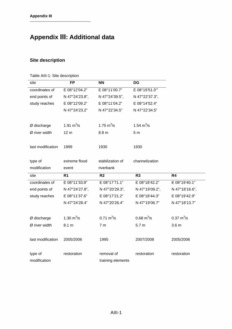
Appendix III: Additional data
Site description
Table AIII-1: Site description
site FP NN DG
coordinates of
end points of
study reaches
E 08°12’04.2”
N 47°24’23.8”,
E 08°12’09.2”
N 47°24’23.2”
E 08°11’00.7”
N 47°24’39.5”,
E 08°11’04.2”
N 47°22’34.5”
E 08°19’51.0’”
N 47°22’37.3”,
E 08°14’52.4”
N 47°22’34.5”
Ø discharge 1.91 m3/s 1.75 m3/s 1.54 m3/s
Ø river width 12 m 8.8 m 5 m
last modification 1999 1930 1930
type of
modification
extreme flood
event
stabilization of
riverbank
channelization
site R1 R2 R3 R4
coordinates of
end points of
study reaches
E 08°11’33.8”
N 47°24’27.8”,
E 08°11’37.6”
N 47°24’28.4”
E 08°17’71.1”
N 47°20’29.3”,
E 08°17’21.2”
N 47°20’26.4”
E 08°18’42.2”
N 47°19’09.2”,
E 08°18’44.3”
N 47°19’06.7”
E 08°19’40.1”
N 47°18’16.6”,
E 08°19’42.9”
N 47°18’13.7”
Ø discharge 1.30 m3/s 0.71 m3/s 0.68 m3/s 0.37 m3/s
Ø river width 8.1 m 7 m 5.7 m 3.6 m
last modification 2005/2006 1995 2007/2008 2005/2006
type of
modification
restoration removal of
training elements
restoration restoration
Appendix III ___________________________________
AIII-2
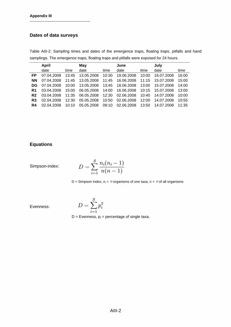
Dates of data surveys
Table AIII-2: Sampling times and dates of the emergence traps, floating traps, pitfalls and hand
samplings. The emergence traps, floating traps and pitfalls were exposed for 24 hours.
April May June July date time date time date time date time FP 07.04.2008 13:45 13.05.2008 10:30 19.06.2008 10:00 16.07.2008 16:00 NN 07.04.2008 11:45 13.05.2008 11:45 16.06.2008 11:15 15.07.2008 15:00 DG 07.04.2008 10:00 13.05.2008 13:45 18.06.2008 13:00 15.07.2008 14:00 R1 03.04.2008 15:00 06.05.2008 14:00 16.06.2008 10:15 15.07.2008 13:00 R2 03.04.2008 11:35 06.05.2008 12:30 02.06.2008 10:40 14.07.2008 10:00 R3 02.04.2008 12:30 05.05.2008 10:50 02.06.2008 12:00 14.07.2008 10:55 R4 02.04.2008 10:10 05.05.2008 09:10 02.06.2008 13:50 14.07.2008 11:35
Equations
Simpson-index:
D = Simpson Index, ni = #organisms of one taxa, n = #of all organisms
Evenness:
D = Evenness, pi = percentage of single taxa.

Appendix III ___________________________________
AIII-3
Vegetation measurements
Table AIII-3: The different vegetation structures included in the vegetation measurements.
vegetation type
1: no vegetation
2: gravel with < 30 % vegetation cover
3: gravel with > 30 % vegetation cover
4: homogenous meadow, regularly cut
5: meadow with additional herbaceous plants, regularly cut
6: meadow with additional herbaceous plants, not cut
7: single young shrub
8: single shrub > 2m high
9: composition of several different shrubs
10: single young tree
11: single tree
12: composition of shrubs and trees, without under story
13: composition of shrubs and trees, with understory
Table AIII-4: Percentage of the different vegetation structures at the different sites.
site 1 2 3 4 5 6 7 8 9 10 11 12 13 FP 18 43 10 5 14 10 NN 8 6 5 5 23 7 19 2 25 DG 75 25 R1 33 15 7 4 25 6 10 R2 4 14 18 4 60 R3 9 61 13 7 3 3 4 R4 4 35 12 12 6 5 26
Appendix III ___________________________________
AIII-4
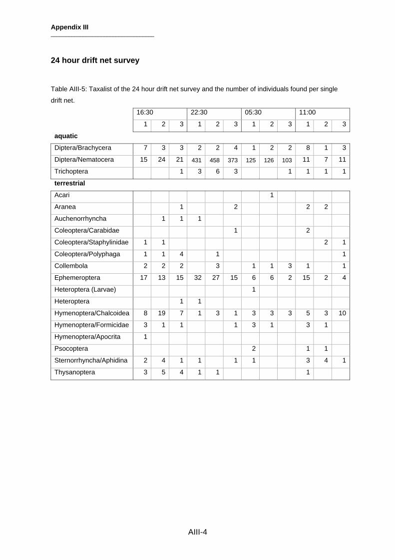
24 hour drift net survey
Table AIII-5: Taxalist of the 24 hour drift net survey and the number of individuals found per single
drift net.
16:30 22:30 05:30 11:00
1 2 3 1 2 3 1 2 3 1 2 3
aquatic
Diptera/Brachycera 7 3 3 2 2 4 1 2 2 8 1 3
Diptera/Nematocera 15 24 21 431 458 373 125 126 103 11 7 11
Trichoptera 1 3 6 3 1 1 1 1
terrestrial
Acari 1
Aranea 1 2 2 2
Auchenorrhyncha 1 1 1
Coleoptera/Carabidae 1 2
Coleoptera/Staphylinidae 1 1 2 1
Coleoptera/Polyphaga 1 1 4 1 1
Collembola 2 2 2 3 1 1 3 1 1
Ephemeroptera 17 13 15 32 27 15 6 6 2 15 2 4
Heteroptera (Larvae) 1
Heteroptera 1 1
Hymenoptera/Chalcoidea 8 19 7 1 3 1 3 3 3 5 3 10
Hymenoptera/Formicidae 3 1 1 1 3 1 3 1
Hymenoptera/Apocrita 1
Psocoptera 2 1 1
Sternorrhyncha/Aphidina 2 4 1 1 1 1 3 4 1
Thysanoptera 3 5 4 1 1 1
Appendix III ___________________________________
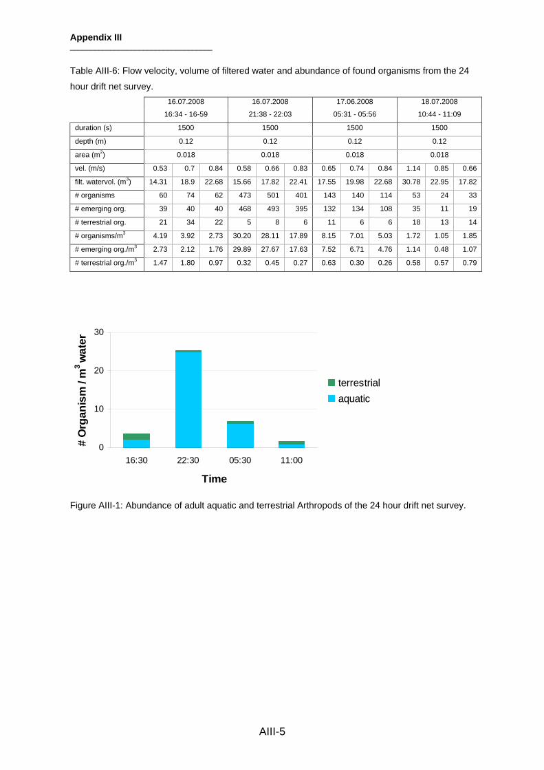
AIII-5
Table AIII-6: Flow velocity, volume of filtered water and abundance of found organisms from the 24
hour drift net survey. 16.07.2008 16.07.2008 17.06.2008 18.07.2008
16:34 - 16-59 21:38 - 22:03 05:31 - 05:56 10:44 - 11:09
duration (s) 1500 1500 1500 1500
depth (m) 0.12 0.12 0.12 0.12
area (m2) 0.018 0.018 0.018 0.018
vel. (m/s) 0.53 0.7 0.84 0.58 0.66 0.83 0.65 0.74 0.84 1.14 0.85 0.66
filt. watervol. (m3) 14.31 18.9 22.68 15.66 17.82 22.41 17.55 19.98 22.68 30.78 22.95 17.82
# organisms 60 74 62 473 501 401 143 140 114 53 24 33
# emerging org. 39 40 40 468 493 395 132 134 108 35 11 19
# terrestrial org. 21 34 22 5 8 6 11 6 6 18 13 14
# organisms/m3 4.19 3.92 2.73 30.20 28.11 17.89 8.15 7.01 5.03 1.72 1.05 1.85
# emerging org./m3 2.73 2.12 1.76 29.89 27.67 17.63 7.52 6.71 4.76 1.14 0.48 1.07
# terrestrial org./m3 1.47 1.80 0.97 0.32 0.45 0.27 0.63 0.30 0.26 0.58 0.57 0.79
Figure AIII-1: Abundance of adult aquatic and terrestrial Arthropods of the 24 hour drift net survey.
0
10
20
30
16:30 22:30 05:30 11:00
Time
# O
rgan
ism
/ m
3 w
ater
terrestrialaquatic
Appendix III ___________________________________
AIII-6
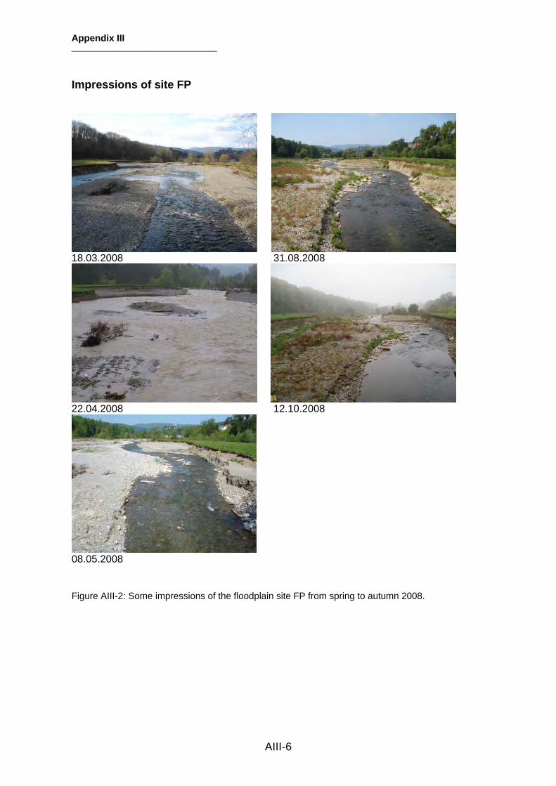
Impressions of site FP
18.03.2008 31.08.2008
22.04.2008 12.10.2008
08.05.2008 Figure AIII-2: Some impressions of the floodplain site FP from spring to autumn 2008.