RReeggiioonnaall PPrriiccee DDiiffffeerreenncceess iinn UUrrbbaann CChhiinnaa

11998866--22000011:: EEssttiimmaattiioonn aanndd IImmpplliiccaattiioonn

Cathy Honge Gong and Xin Meng1

Abstract

Despite the intensive efforts made by economists to examine regional income inequality in China, limited attention has been paid to disentangle the contribution of regional price differentials. This paper examines regional price differential in urban China over the period 1986 to 2001. Spatial Price Index (SPI) is normally calculated using the Basket Cost Method, which defines a national basket and measures price variation of this common basket across different regions. The weakness of this method is that it arbitrarily assumes consumers’ preferences and has a strong reliance on good regional level price data, which are often not available. This paper adopts the Engel’s curve approach to estimate a Spatial Price Index for different provinces. The SPI obtained from the Engel’s curve approach indicates larger regional price variations than those obtained from the Basket Cost method. Further, regional price variations in urban China increased significantly during the late 1980s to early 1990s, stabilized at a relatively high level during the mid to end 1990s. Adjusting for the regional price variations our finding suggests that regional income inequality increased the most between the late 1980s and early 1990s, and stabilized in the mid 1990s, which contradicts previous findings using unadjusted income.

JJEELL CCllaassssiiffiiccaattiioonn:: CC4433,, EE3311,, PP3366 DD1122

KKeeyy WWoorrddss:: SSppaattiiaall pprriiccee iinnddeexx;; EEnnggeell’’ss ccuurrvvee,, IInnccoommee iinneeqquuaalliittyy,, CChhiinnaa..

1 Economics Program, Research School of Social Sciences, The Australia National University; Canberra ACT 0200, Australia, E-mails: cathy.gong@anu.edu.au, xin.meng@anu.edu.au

RReeggiioonnaall PPrriiccee DDiiffffeerreenncceess iinn UUrrbbaann CChhiinnaa 11998866--22000011::

EEssttiimmaattiioonn aanndd IImmpplliiccaattiioonn

1. Introduction A Spatial Price Index (SPI) reflects price differences across different regions

at a point in time. Regional price differences or inter-area comparisons of the cost of

living are very important in measuring poverty and income inequality, analyzing

regional labor markets and comparing employee compensation cost, and for making

location decisions for business and households (Kokoski, 1991, Moulton, 1995, Hayes

2005). Studies have found that measurement of poverty rates and regional income

differentials are very sensitive to regional cost of living adjustments (Johnston,

Mckinney, and Stark , 1995; Short, 2001; Slesnick, 2002; Jollife, Datt and Sharma,

2004; Brandt and Holz, 2007; Dalen, 2006; Roos ,2006; Jolliffe, 2006).

In the last two decades, China has experienced a significant increase in

regional inequality of income and regional income disparity has become an important

policy issue (Knight and Li, 1999; Khan and Riskin, 2001; Riskin, Zhao, and Li,

2001, Meng, 2004; Benjamin, Brandt, Giles, and Wang, 2005). The question naturally

arises as to how much of the regional income inequality is due to an increase in real

income inequality and how much is due to an increase in regional price variation.

Despite the intensive effort made by economists to examine regional income

inequality, limited attention has been paid to disentangling the relative contributions

of real income inequality and regional price differentials.

Regional price differences are normally greater in a developing country with

segmented markets than in a developed country where there exists a higher degree of

market integration. China has had a long history of market segregation and the extent

of its regional price differentials is widely recognized (Young, 2000; Fan and Wei,

2006; Braddon and Holz, 2005; Jiang and Li, 2005). Based on price data collected by

the National Bureau of Statistics in 1997 a simple average of consumer prices for

tradable goods in the province with the highest prices is 4 times that of the lowest

price province. For the non-tradable goods and services the price ratio is 9 times

1

(NBS, 1998). 2 Such large regional price dispersion makes it difficult to study changes

in regional inequality and poverty without adjusting for spatial price differentials.

In the economic literature, a “Spatial Price Index (SPI)” is often derived

through specifying a basket of goods and services and pricing this basket in different

localities (Sherwood, 1975; Kokoski, 1991, Deaton, 2003). This method is referred to

as the Basket Cost method hereafter and it requires price data for the same bundle of

same quality goods to be collected for different regions. Such data are normally not

available. Many studies, therefore, use price data collected for constructing an inter-

temporal Consumer Price Index. These price data are not directly comparable across

regions because they are not specified as the same brand or quality across regions

(Kokoski, 1991). In response to this shortcoming, Kokoski, Moulton, and Zieschange

(1999) developed a hedonic regression method which adjust regional differences in

quality of goods to derive a set of bilateral inter-regional price indices for each good

and from which SPI may be derived (Koo, Phillips, and Sigalla ,2000 and Slesnick,

2002). In most developing countries, however, detailed price data are not available or

only available for some years and not others. In the absence of detailed price data,

Deaton (2003) developed a unit value approach to derive prices from household

expenditure. This approach is also not ideal as unit values are often biased due to

measurement error, quality inconsistency and unavailability of prices for non-

purchased goods (Deaton, 1997; Gibson and Huang and Rozelle, 2002; Gibson and

Rozelle, 2005; Dalen, 2006).

Recently, Hamilton (2001a) and Costa (2001) use cross-sectional household

survey data and the Engel’s Curve approach to estimate the CPI bias over time in the

U.S. The basic idea is quite simple. Because Engel’s law is regarded as the best

established economic law, movements in the budget share of food could serve as an

indicator of movement in real income. If real income as indicated by Engel’s law is

different from real income as measured by nominal income deflated by the CPI, one

may be able to estimate the extent to which the CPI is biased. Hamilton (2001a)

suggests that this method could be extended to estimate the movement in a true cost-

of-living index for different races, age groups, geographic areas, and for developing

countries with adequate household survey data.

2 Data are reported in Appendix A.

2

There have been only a few studies on regional price differences in China due

to lack of published regional price data (Young, 2000; Jiang and Li, 2005; and Brandt

and Holz, 2007). To the best of our knowledge, Brandt and Holz (2007) is the only

comprehensive study which derives a set of Spatial Price Indices for China. Using one

of the few available provincial level price data, they calculated the SPIs for the year

1990 for rural and urban China across provinces and then adjusted these spatial price

indices by regional inter-temporal changes in the CPIs for the years between 1984 and

2002. Due to data limitation, however, their estimation may suffer from various

biases. These possible biases include: (1) the 1990 price data were collected for the

purpose of calculating CPI, which have no quality adjustment across different regions;

(2) the 1990 urban price data used only record provincial capital cities, rather than

average price level in all cities in each province; (3) as there was no record of prices

for non-tradable goods, average manufacturing wages were used as proxies; (4) the

SPIs for years rather than 1990 were obtained from using provincial CPI to deflate

1990 SPI. However, CPI uses the base year provincial average consumption bundle as

the weights while SPI is supposed to use current year national average consumption

bundle as weights. In addition, CPI series itself may be biased (Erwin, 1996;

Moulton, 1996; Boskin et al, 1998; Nordhaus, 1998; Lebow, 2001; Meng, Gregory,

and Wang, 2005).3

In light with the problem associated with lack of proper price data, in this

paper we follow Hamilton’s suggestion to extend the Engel’s curve approach to

estimate a new series of Spatial Price Index for different provinces for urban China.

The data used are from the China Urban Household Income and Expenditure Survey

for the period 1986 to 2001. The Engel’s curve approach may be considered as more

appropriate than the Basket Cost method in estimating SPI for this period in urban 3 Normally, the base year provincial level bundles differ considerably from the national current year bundle. The longer the time period the more they deviate from the national average current year bundle. Because of this deviation, SPI calculated using the base year SPI deflated by provincial level CPI will also deviate from the SPI series which is calculated using each year’s price level and national consumption bundle. Appendix B presents some results from an exercise which uses the provincial level price data for the year 1991-1997 (NBS,1998) and the provincial CPI series over the same period to calculate two sets of SPI: one uses Brandt and Holz (2007) method which calculate the 1991 SPI and deflate it using provincial level CPI over time (noted as DSPI hereafter) and the other uses each year’s price data to calculate SPI (noted as ASPI hereafter) separately. The results show that in 1992 (the first year of deflation) there are slight differences in the price ratio of for the highest and lowest provinces, standard deviations, and Coefficient of Variations, between DSPI and ASPI. The correlation coefficient for the two series in 1992 is 0.96. The discrepancy increases over time. By the end of the period, 1997, the correlation coefficient for the two series reduced to 0.60. Using

3

China for the following reasons. First, the normal Basket Cost method superimposes

a constant national basket on different regions. It does not take into account regional

preference differences. For example, suppose that one region is dominated by Muslim

who do not consume pork, but at the national level pork is one of the most commonly

consumed meat and hence is included in the basket, the national cost of living basket

will not be representing the Muslim region's preference. The Engel’s Curve approach,

on the other hand, infers cost of living directly from consumer’s behaviour. Second, in

a period of economic transition, the price of the national cost of living basket may not

be straightforward. During the 1990s urban Chinese households experienced

extraordinary changes in income, price and social welfare provisions. These changes

were introduced at different points in time to different regions. These changes

effectively changed people’s true cost of living. The following example may explain

this situation more clearly. Suppose that the price level of a certain medicine is 10

yuan in region one and 11 yuan in region two (10 per cent difference). If 80 per cent

of consumers in region one has full public health cover while 50 per cent of

consumers in region two has 40 per cent public health cover, the actual price

difference of this medicine between region one (10 yuan times 20% equals 2 yuan)

and region two (11 yuan times 50% time 40% plus 11 yuan times 50% equals 7.7

yuan) is not 10 per cent but 285 per cent. Normally price level data do not distinguish

the extent to which the price of same medicine differs under different systems,

whereas the Engel’s curve approach take this into account by inferring the true cost of

living directly from consumers’ behaviour.

The paper is structured as follows. Section 2 describes the historical reasons

for the existence of significant regional price differentials in China. Section 3

introduces the Engel’s curve approach and the model used in this paper. Section 4

describes the data and summary statistics. Section 5 presents the main results from the

Engel’s Curve approach. Section 6 calculates SPI using the Basket Cost method with

price data that are available for a few years and with unit values for the whole study

period. Section 7 compares the SPI from different approaches. Section 8 investigates

how regional income inequality may differ after adjusting SPIs estimated by the

Engel’s curve approach. Conclusions are given in section 9.

4

2. Background There are significant price differences across Chinese regions. This is a widely

accepted fact (Young, 2000; Fan and Wei, 2006; Braddon and Holz, 2007; Jiang and

Li, 2005). Based on an internal publication on prices of 120 tradable and non-tradable

goods (NBS, 1998),4 Appendix A presents the ratio for the simple average of

consumer prices of the tradable goods in a highest price province to that in a lowest

price province and the same ratio for non-tradable goods between 1991 and 1997. It

shows that in 1991 the ratio for tradable goods is about 3.5 times, it increased slightly

in 1993, reduced somewhat in 1994, and finally reached 4.2 times in 1997. For non-

tradable goods the ratio is much higher, ranging between 8.73 times in 1991 to 9.01

times in 1997. Although these data may not accurately reflect regional price

differentials due to the fact that these data were collected for the purpose of

constructing inter-temporal CPI and hence may reflect different quality of goods, they

do provide an indication of the regional price variations. To better control for quality,

table 1 presents data on selected goods which may subject to less quality variation.

These data also show significant regional differentials.

What are the reasons for such a large regional price variation in China? In a

study of international price deviations from purchasing power parity (PPP), Cecchetti,

Mark and Sonora (2002) suggested the following reasons: (1) trade barriers; (2)

bureaucratic difficulties; (3) local monopoly power; (4) transportation costs; (5) the

failure of nominal exchange rates to adjust to relative price level shocks; (6) sticky

nominal price-level adjustment because price changes are costly; (7) the presence of

non-tradable goods and services and the potential for different growth level and

efficiency of factors used in production. Although Cecchetti et al.’s (2002) summary

is focused mainly on cross country price differentials, it is also applicable to regional

price differentials within a particular country as long as these conditions exist, and

more specifically, there exists regional protectionism. China’s regional protectionism

has long been recognized (Young, 2000; Bai, Du, Tao and Tong, 2003). Thus, these

are all relevant reasons for large regional price differentials in China.

4 Note that these are the only available data which provide information at provincial level with both prices for tradable and non-tradable goods.

5

In addition to the reasons listed above, China’s special development strategy

and its gradualist economic reform process may also have contributed to the large

regional price variations. Below we outline some of the important reasons.

First, economic development in different regions varies considerably not only

due to the unequal distribution of natural resources and regional difference in

proximity to major markets, but also due to government deliberate policy initiatives.

During the cold war era the government purposely established heavy industry in

inland cities and light industry in coastal cities (Jian, Sachs and Warner, 1996). Later,

at the earlier stage of economic reform, coastal regions received many preferential

policies from the central government, which provided more opportunities for these

regions to grow faster and further widened the economic growth gap between costal

and inland regions (Cai and Wang, 2003). As a result, the coastal regions have higher

labor productivity and per capita income, which has increased demand for consumer

products and services, and generally increased the price level, especially for services.

Second, the imperfect mobility of labor and capital among regions can

differentiate the returns to factors and cause regional price disparities. During the pre-

reform era, labour mobility was strictly forbidden and implemented through the

household registration and food ration systems. Individuals born in one area moved to

another area who would not be registered and would not receive food coupons, and

hence could not survive (Jian and Sachs and Warner, 1996; Meng, 2000; Whalley and

Zhang, 2004). Capital allocation was controlled strictly by central government

through the central planning system (Jian, Sachs and Warner, 1996). Since 1978, the

introduction of the market-oriented reform and open-door policy has increased the

movement of factors among regions, which is expected to narrow regional price

disparities (Cai and Wang, 2003). However, large foreign investment entering into the

eastern region has increased the capital-labor ratio in this region, and the household

registration system still hampers nation wide labor market integration under the

current “guest” working system (Meng and Zhang, 2001; Zhao, 1999; and Du,

Gregory, and Meng, 2006). Consequently, regional prices may converge more slowly

than expected.

Third, local protectionisms, including trade barriers, bureaucracy difficulties

and local monopoly, play a unique role in regional price disparity in China through

differential pricing to segmented markets and making trade and market entrance more

6

difficult. China’s economic reform since 1978 has introduced fiscal decentralization,

which provided local governments with a strong incentive to shield local firms and

industries from interregional competition, especially for those industries that had high

tax-plus-profit margins in the past. Meanwhile, there was no promulgation in the early

years of economic reform, and no effective implementation in the later years, of

central-government policies that prohibit trade barriers (Bai, Du, Tao and Tong,

2003). Therefore, local protectionism has a significant effect on the degree of regional

price difference by introducing monopoly profits and additional costs into prices.

Local protectionism in China includes numerous local standards, regulations and

customs covering everything ranging from cars to construction materials, fertilizer to

instant noodle and beer and even satellite television programs (People’s Daily, July 01,

2000). “Silkworm cocoon war” and “car war”’ are two typical interregional trade

conflicts in raw materials and finished manufactured goods in the 1980s and 1990s

(Young, 2000 and Bai, Du, Tao and Tong, 2003).

Finally, the dual track and gradual price reform affected regional prices

through geographical difference in industrial structure. Before economic reform, most

commodities in China were priced through the central planning system. After 1978,

the State gradually allowed the market determination of prices (NBS Internal Statistic

Report, 2000; Fan and Wei, 2006). From 1979 to1983, controls on prices of major

agriculture goods and industrial inputs were gradually adjusted upwards to their

market price levels. For instance, purchase prices of farming products increased by

more than 20 per cent, which led to a 30 percentage point decrease in the price ratios

of farming products to industry products. With the progressive price decontrol, the

purchasing prices were completely decentralized by 1992, and by 1999, 95 percent of

consumer goods and 80 percent of investment goods were priced by the market (NBS

Internal Statistic Report, 2000; Fan and Wei, 2006). During the whole period of price

reform, especially in the years with high inflation rates, the regional prices diverged

significantly because of the regional difference in industrial structure.

3. Methodology The most commonly used Basket Cost method, either with regional price data

or unit values, suffers from two problems. First, it imposes a fixed basket on

consumers from different regions and ignores differences in environment and

preferences. Second, it has an extremely high requirement for price data (or unit value)

7

on a particular good to have a same quality across different regions. This requirement

is often very difficult to satisfy. To mitigate these problems, this paper extents a

newly developed Engle’s Curve approach (Nakamura, 1996, Hamilton, 2001, Costa,

2001, and Gibson, Stillman, and Le, 2004) to estimate a new series of Spatial Price

Index for urban China.

One of the most important generalizations about consumer behavior is that the

fraction of income spent on food tends to decline as real income increases. This

finding was first discovered by the Prussian economist, Ernst Engel (1821-1896), in

the nineteenth century and has been known as Engel’s Law. Engel’s Law states that

the food budget share is inversely related to household real income and food has

positive income elasticity, which is less than 1. Engel’s Law is probably one of the

best economic laws observed in economic data and has been confirmed by recent

consumer data of many countries (Houthakker, 1987; and Hamilton, 2001).

The basic idea of using Engel’s Curve to estimate CPI bias is as follow. With

proper model specification and reasonable assumptions, there should not be

systematic movement in the Engel’s curve over time (or across regions). If the

Engel’s curve moves, it implies that the real income is not measured correctly, which

in turn indicates that the price index used to deflate real income is biased. However,

Engel’s Law can be used to infer the movement of real income only when other

factors, such as changes of relative prices and household characteristics, are held

constant.

Hamilton (2001) uses the single-good demand function in Almost Ideal

Demand System (AIDS) developed by Deaton & Muellbauer (1980) as the theoretical

platform for Engel’s curve approach to estimate CPI bias. His approach is to estimate

an augmented Engle’s curve as follows:

tj,i,x'

tj,i,tj,tj,i,tn.j,tj,f,tj,i, μθΧ]lnpβ[lny]lnpγ[lnpcω ++−+−+= (1)

where ωi,j,t is the food budget share of household i living in region j at time t; pf,j,t,

pn,j,t, and pj,t are the unobserved true price indices for food, non-food, and all goods in

region j in time t, respectively; yi,j,t is nominal expenditure of household i living in

region j at time t; Xi,j,t is a vector of household characteristics; while μi,j,t is the

residual. The first item in equation (1), ]ln[(ln ,,,, tjntjF pp −γ , can be treated as the

8

substitution effect between food and non-food, and the second term,

]plny[ln t,jt,j,i −β , can be treated as the income effect. It is assumed:

(1) The price of all goods is a weighted average of the food and non food prices:

=tjp ,ln tjntjF pp ,,,, ln)1(ln αα −+ (2)

(2) As the true prices are unobserved, the CPI series are used to proxy the true prices.

Thus, all true prices t,j,nt,j,f p,p and tjp , are measured with errors:

)E1ln()1ln(plnpln t,jt,j0,jt,j ++++= Π , (3a)

)E1ln()1ln(plnpln t,j,Ft,j,F0,j,Ft,j,F ++++= Π (3b)

)E1ln()1ln(plnpln t,j,Nt,j,N0,j,Nt,j,N ++++= Π (3c)

where Π is the cumulative increase in the CPI measured price (of food, nonfood, or

all goods), and Et is the year t percent cumulative measurement error in the CPI since

year 0. Substituting equations (3a) to (3c) into equation (2), gives:

)E1ln()1()E1ln()E1ln( t,j,nt,j,Ft,j +−++=+ αα (4)

Substituting equations (3a) to (3c) and (4) into Equation (1), gives

t,j,i0,j

0,j,N0,j,Ft,jt,j,Nt,j,F

t,jt,j,it,j,nt,j,ft,j,i

pln)plnp(ln)E1ln()]E1ln()E1[ln(

'X)]1ln(Y[ln)]1ln()1[(ln(

μβ

γβγ

θΠβΠΠγφω

+−

−++−+−++

++−++−++= (5)

Let:

)E1ln()]E1ln()E1[ln( tt,Nt,Ft +−+−+= βγδ and

)E1ln()]E1ln()E1[ln( jj,Nj,Fj +−+−+= βγδ ,

and assuming that the CPI bias does not vary geographically, equation (5) may be

written as:

∑ ∑= =

++++

+−++−++=T

1t 1jijtjjtt

'

t,jt,j,it,j,nt,j,ft,j,i

DDX

)]1ln(Y[ln)]1ln()1[(ln(

μδδθ

ΠβΠΠγφω (6)

where, tδ and jδ are the coefficients of time and regional dummy variables tD , and

jD , respectively. The parameter estimated from (6) can be used to identify the CPI

bias as:

9

)

)k1(1)k1(exp(1E t

t

−−−

−−−=−

αγβ

δ (7a)

where k is the relative bias between food and nonfood prices. Further assuming food

and nonfood prices are equally biased, k=1, then )E1ln(k)E1ln( t,Nt,F +=+ and

equation (7a) can be written as:

)exp(1E tt β

δ−−=− (7b)

Thus, under the assumptions that the demand function is properly specified,

preferences are stable, there are no systematic errors in the variables, and food and

nonfood prices are equally biased, the error in the CPI can be identified by

coefficients, δ and β, obtained from estimated equation (6) using pooled repeated

cross-sectional household expenditure survey data.

We can also use Engel’s Curve Approach to derive SPI. To do so, we can

estimate Equation (6) using one cross-sectional data at a time. Since the true food

price ( j,fp ) and non-food price ( j,np ) for each province are not available, we use

aggregated unit values for food ( j,fΠ ) and non-food ( j,nΠ ) to proxy for the true

prices, respectively with measurement errors. Assuming that the unit values of food

and non food for each province at a point in time have the same level of measurement

error, ( 0)ElnE(ln t,j,nt,j,f =− ), provincial dummy variables can be used to capture

provincial general price effects. In order to more precisely capture substitution effects

between food and non-food and to avoid multicollinearity between relative food/non-

food prices and the general price effect (provincial dummy variables) in the model,

we use aggregated unit values at city level for food ( c,fΠ ) and non-food ( c,nΠ )

instead of those at provincial level. Thus, the final estimated equation is specified as

follow:

j,ijjj,ij,c,nj,c,fj,i 'XD]Y[ln)]ln()[(ln( μθδβΠΠγφω ++++−+= (8)

In equation (8), the omitted province is Beijing, for which the general price

effect 1φ is captured in the constant term φ and cannot be identified directly. If we

express the price of Beijing relative to the national average price level

as )exp(p 11 β

φ−

= , and the relative price of province j to the national average price

10

level as )exp()exp(p 1jjj β

φδβφ

−+

=−

= as the difference between the general price of

other provinces j and that of Beijing is ( 1jj φφδ −= ), the relative price level of

province j to Beijing can be calculated as:

)exp()exp(/)exp(SPI j11jj β

δβφ

βφδ

=−−

+= (9)

To estimate equation (8), we use the budget share of food at home rather than

that of all food as dependent variable. This is because that eating-out is expected to

have different income elasticity from food at home and that food at home is mainly to

satisfy the basic requirement of nutrition intake while eating out can be treated

partially as luxurious consumption or recreation.

In the literature, y is either measured in terms of income or expenditure.

Although we use both income and expenditure in our estimated model, it is worth

noting that using expenditure may provide more stable results due to three reasons.

First, annual household income can be erratic and unpredictable, especially for self-

employed and family businesses. In the household survey data, some households are

found to have income less than their food consumption or even negative annual

income. Second, expenditure is typically a better guide to long-term wellbeing of the

household as households will exercise some consumption smoothing through savings

and dissavings (Deaton, 1997). Lastly, expenditure is often measured with less error

than income in household surveys, although with the nature of the data used in this

study, e.g. diary records, they both should be reasonably accurate.

One weakness of using coefficients on regional dummy variables to infer

regional price variations is that other cross regional variations may confound the price

effect (Hamilton, 2000a). To this end, inclusion of relative food/non-food price may

pick up some of the cross-regional variations in the food budget share. Another

important variable which affects individuals’ food budget share is personal taste

difference across regions. If there is no systematic preference variation across

different provinces, ignoring preference differences may not bias our results. However,

it is commonly known that Chinese provinces have considerable preference variations

with regard to food. Although it is hard to capture regional taste difference

empirically, health and nutrition literature has long established that weather,

11

especially temperature, has a significant impact on diet and food preferences

(Stroebele and Castro, 2004; and Thompson and Wilson, 1999). In this paper,

therefore, we use city level temperature and its squared term to capture possible

dietary differences across regions.

Following the literature, other exogenous control variables in vector X include

the age of household head and spouse, their education level, household size, and a

group of variable indicating household composition, such as the female ratio of

household members, the number of children between age 0-15, and the number of

household members over 65. The share of eating out in all food expenditure is also

included in the model.

Whether the Engel’s curve approach is suitable for deriving the SPI in China

depends on whether the assumptions made in deriving the result in equation (9) are

reasonable. While four substantial assumptions are required to use the Engel’s Curve

Model to estimate CPI bias over time,5 only one assumption is required to estimate

the SPI. This assumption is that the proxies for food and non-food prices have

constant measurement errors for each province and at a point in time. This assumption

should be largely satisfied. Appendix C shows the possible bias it may bring to our

estimation of the SPI if this assumption is violated.

44.. Data and Summary Statistics The data used in this study are from the China Urban Household Income and

Expenditure Survey (UHIES) for the year 1986 to 2001. The surveys are conducted

by the Urban Survey Organization of National Bureau of Statistics in China (USO,

NBS). The UHIES covers 30 provinces. The survey samples households with urban

household registration in each province.6

The sampling and survey methods of UHIES have been relatively consistent

over time. The sample is selected based on PPS with several stratifications at the

provincial, city, county, town, and neighborhood community levels. Households are

randomly selected within each chosen neighborhood community. Each household is

5 The assumptions are: 1. The structure of the model is stable over time so that cross-section data can be pooled. 2. Food and non-food CPI is biased constantly or equally over time. 3. CPI bias does not vary geographically. 4. There is no significant time trend in food consumption. 6 Before 1988 there were only 29 provinces in China. In 1988 Hainan province was established and in 1997 Chongqing was established. Tibet is not included. Migrant workers who possess rural household registration and working in cities are not included in the survey.

12

designed to be in the sample for one to three years. All households are designed to

have equal weights in each year.

The main data collecting method are diary records of income and expenditure,

where households are required to record each item (disaggregated for hundreds of

product categories) purchased or income received for each day for a full year.

Enumerators visit sample households once or twice each month to review the records,

assist the household with questions, and to take away the household records for data

entry and aggregation to the annual data in the local Statistical Bureau Office (Han,

Wailes, and Cramer, 1995; Fang, Zhang, and Fan, 2002; and Gibson, Huang, and

Rozelle, 2003; Meng, Gregory and Wang, 2005). Only annual household aggregated

data are used in this paper.

The total number of households in the survey ranges from 12,000 to 17,000

with around 47,000 to 53,000 individuals each year. Excluding missing values and

incorporating a few sample restrictions the final samples used are between 11266 and

16121 households. Table 2 presents the sample size for the original total sample and

the restricted sample for each year.7

UHIES collects data on income, expenditure, housing condition, durable

goods possession and demographic characteristics. The UHIES questionnaire has

changed twice during the data period from 1986 to 2001. The major changes in

questionnaire occurred in 1988 and in 1992.8 Consequently, some discontinuity in the

data series may exist and may affect the estimation. In addition, UHIES do not

provide information on self-produced goods for own consumption, gifts from others,

7 The sample restrictions include: (1) Tibet is excluded from the data because only 100 households are included in a few years. Hainan and Chongqing provinces were established in 1988 and 1998 and the data were not available until 1990 and 1998, respectively. (2) households with negative values on food consumption, eating out, or consumer durables, or with outliers in income/expenditure and with more female members than total household members are excluded. (3) households in Wuwei city of Gansu province in 1986, Bijie city of Guizhou province in 1988, Shanggao city of Jiangxi province in 1988, and Si-Ping city of Jilin province in 1998 seem to have serious measurement errors on quantity data and are therefore excluded from the final sample. (4) households with their heads younger than 18 or with more than 8 individuals are excluded. These restrictions exclude between 4.2% to 9.4% of the total sample in each year. We also estimate the equations with the full sample and the results do not vary much. The full results of these tests are available upon request from the authors. 8 The major changes made in 1988 are related to income sources. Before 1988, only total monthly wages for individuals are collected, while after 1988, individuals’ income from different sources, such as wages, household business, property and transfers are collected. The main changes to the questionnaire made from 1992 are related to the consumption categories. Prior to 1992 there are 39 food goods, 39 non-food goods and 13 service categories are included in the UHIES surveys. Since 1992 the questionnaire includes 113 food, 131 non-food g, and 25 services categories.

13

state subsidies on various goods, and imputed rent for owner-occupied housing. The

lack of the above information may also affect the calculation of SPI.

The mean and standard deviation of income, expenditure, food budget share,

relative food price, and other variables used in our estimation for all years are

presented in Table 3. On average the budget share of food at home reduced from 46

per cent in 1986 to 31 per cent in 2001, while the eating out budget share of the total

food budget increased from 5.5 per cent to 13.9 per cent over the same period. In

addition, Table 3 shows that household and individual characteristics have also

changed. The average household size and the number of children aged between 0 and

15 fell which is consistent with the implementation of the one child policy. The

average age of household head increased by almost 5 years, while years of schooling

for husband and wife increased by 1.6 and 1.9 years, respectively. The summary

statistics by provinces in all years, which are available upon request from the authors,

indicate obvious regional variations of all variables, especially in income, expenditure,

food budget share and eating out between rich provinces (e.g. Beijing or Guangdong)

and poor provinces (Shanxi or Henan).

It is expected that at the same level of income/expenditure, different provinces

should have a similar food budget share. However this does not hold in the data.

Figure 1 shows the relationship between the budget share of food at home and log

nominal expenditure for selected provinces and selected years. It indicates that at each

expenditure level, the food budget share differs considerably among different

provinces and the situation persists for all the years. This is a strong indication that

price level differs considerably among provinces, and hence, real income/expenditure

adjusted by spatial price differences differs considerably from the unadjusted

income/expenditure.

5. Estimated results

5.1 Results The results from estimated Equation (8) are presented in Table 4. The overall

significance of the regression model is relatively high with the adjusted R-square

ranging from 0.44 to 0.60.

Expenditure plays a significantly negative role in determining the food at

home budget share. For each year the coefficient is statistically significant at the 1 per

14

cent level. This result is consistent with Engel’s Law. Over time, however, we

observe that the magnitude of the effect of expenditure on the food at home budget

share decreased significantly, from 18.7 per cent in 1986 to 14.1 per cent in 2001. We

also calculate the expenditure elasticity of food at home budget share for each year,

which are presented in Table 5.9 The elasticity falls from 0.59 in 1986 to 0.54 in 2001

as income rises, which means that in 1986, 1 percent increase in total expenditure

generated a 0.59 percent increase in food at home, and this ratio reduced to 0.54 per

cent in 2001. The reduction is not huge and even in 2001 the elasticity is far from zero

and way above the elasticity for the U.S. for the year 1974, which is estimated to be

0.33 (Hamilton 2001). The relative food price plays a mixed role with some positive

and some negative effects on food at home budget share over time. Eating out as the

share of food budget contributes negatively and significantly to the food at home

budget share.

The linear temperature variable plays a consistent important role in food

budget share over the whole period, while its squared term is only statistically

significant in some years. Most variables related to household characteristics and

composition are statistically significant in most years. For example, the coefficients of

family size are all positively significant implying the larger the household the higher

the food budget share at home. Number of children aged 0 to 15 do not have a

consistent impact on food at home budget share for reasons which are not clear to us.

Households with more elderly aged over 65 consume more food at home, and age of

household heads and spouses have positive effects on the food budget share at home.

Finally, the years of schooling of both household heads and spouse have a negative

and significant effect on food at home budget share. This could indicate both income

effect (more educated people earn more) and/or a physical activity effect (educated

people are more likely to have a sedentary job, which requires less energy

consumption).

Turning to the most important results for this paper—the coefficients for

provincial dummy variables and their implied spatial price indices for different years,

we find that most coefficients are statistically significant at the 1 or 5 per cent levels.

In the regression, Beijing is the omitted category. Thus, the calculated SPI is the

relative price level of other provinces to Beijing. The calculated SPI for all the years 9 The formula used to calculate the expenditure elasticity of food at home is ωβη += 1F,y

.

15

are reported in Table 6. At the bottom of the table the maximum, minimum, mean,

standard deviation and coefficient of variation of the SPI are reported. In addition, the

year to year correlation coefficients, and correlation coefficient of each year relative

to the base year, 1986, are also reported.

Table 6 reveals several important findings. First, there is some persistence in

the provincial relative price position over time. For example, the commonly observed

high price provinces are Guangdong, Shanghai, Tianjin, Beijing and Fujian, while low

price provinces include Shanxi, Shaanxi, Henan, Hebei, and Yunnan. This can also

been observed in Figure 2, where rankings of the relative price position for 1986,

1995 and 2001 are presented. In addition, the year-to-year correlation coefficients and

relative to base year correlation coefficients also show a relatively high correlation of

the relative price position over time. The observed high price provinces seem to

coincide with common knowledge that large cities and more economically advanced

regions often have higher living costs. With regard to low price provinces it is unclear

a priori whether they are reasonable or not.

Second, a few significant changes in the provincial relative price position over

time are observed. For example, as indicated in Figure 2, at the beginning of the

period Shandong province had a relatively high price level, while at the mid 1990s its

relative price level reduced dramatically and stayed low until the end of the period.

Such instability in the relative price position, fortunately, is rare.

Third, the trend of the dispersion of prices over the years seems to have

changed. Figure 3 presents the mean and coefficient of variation of the SPI for the

whole period. It indicates that at the beginning of the period, the dispersion was

relatively low, but increases continuously until 1993, with exception of 1992, then

after 1993, the dispersion seems to stablise at a relatively high level.10

The trend of price dispersion across provinces seems to suggest that between

the late 1980s and the early 1990s price dispersion increased the most and during the

period of the most significant economic reform (1993-1997) urban China actually

experienced largest regional price variation. This, to some extent, seems in conflict

with the objectives of the economic reform agenda. It is often considered that the real

economic reform in urban China occurred after 1992, when Deng visited the South 10 The reason for the significant reduction in price dispersion in 1992 is not entirely clear to us, except that both Young (2000) and Brandt and Holz (2007) find the same phenomenon.

16

China and the government announced that the market system was compatible with

Chinese socialism (Jaggi, Rundle, Rosen, and Takahashi, 1996; Wu, 200?). Since then

the private sector has grown significantly and foreign direct investment, exports, and

GDP increased dramatically. One would think that the privatization process should

have reduced regional protectionism, which, in turn, would reduce regional price

differences.

How should we reconcile our findings of large regional price variations in the

mid to late 1990s with the 1990s’ economic reform agenda? Two possible

explanations may be presented. First, Young (2000) also observed the highest

industrial price variations during the mid to late 1990s. His explanation is mainly

related to local officials’ rent seeking behaviour. If local officials’ promotion is

related to their GDP level, which, in turn, is related to the development of some

particularly profitable manufacturing goods, one would observe convergence in the

structure of production. To protect local production from competition of similar

products of other regions, local protectionism bound to rise, and hence, a high level of

regional price variation would be observed. Anecdotal evidences as indicated in

Young (2000), Bai, Du, Tao and Tong (2003) and numerous newspaper articles seem

to support this explanation.

Another explanation, which may be more closely related to our finding of high

spatial consumer price variations, is perhaps related to the intensive social welfare

reforms introduced in the mid to late 1990s. In the pre-reform era and up until the late

1980s urban Chinese were largely covered by a cradle-to-grave welfare system,

whereby education, health care, housing, and many other forms of services were

provided free of charge or at highly subsidized prices. Starting from the early 1990s,

schools began to charge fees, then health care, housing, and most other forms of

former free services were subject to different forms of fee charging. Some were

subject to public sector fee charges, while others were operated in the market places

completely. Different regions had different levels and types of charges. This may

explain, to a large extent, the high regional price variations during this period. By the

end of 1990s, majority of these goods and services were provided in the market place,

and consequently, regional price variations reduced slightly and stayed at that level.

17

5.2 Sensitivity tests In the above analysis the food at home budge share is measured as food share

in total expenditure while y in equation (8) is measured as log total expenditure.

Regressions using food at home as share of total income as the dependent variable and

log household income as the measure of y are also estimated for each of the survey

years. In addition, we also use the unrestricted sample. In general, the results are quite

consistent and the estimated SPI series has the same trend, though the magnitudes

vary somewhat. Regressions using the budget share of all food (food at home plus

eating out), disposable income, and regressions excluding families of single adult or

single parent are also estimated and the estimated SPI do not change significantly.11

6. SPIs Calculated Using the Basket Cost Method with Prices level data and Unit Value Data

In addition to the SPI estimated from the Engel’s curve approach, we also

calculate two other SPI series, one using limited available provincial level aggregated

price level data and the other using unit value data generated from UHIES 1986-2001.

6.1. Using Provincial Average Price Data The provincial average retail price level data for 1991 to 1997 (PARP 1991-

1997, hereafter) used in this study were aggregated by China’s National Bureau of

Statistics (NBS) using the original price data collected from 260 survey cities (NBS,

1998). The initial purpose to aggregate the price data is to compare CPIs calculated

using two different methods—the chained Laspeyres CPI index implemented before

2001 and the new 5-year fixed bundle Laspeyres CPI used since 2001. The data set

covers prices of 120 goods and service categories in food (without prices of

vegetables and fruits), alcohol and tobacco, clothing and footwear, housing costs

(electricity, house repairs and maintenance, self building materials, housing rent),

household contents and services, health, transportation, communication, recreation

and education. The list of these goods and service categories is listed in Appendix A.

The PARP 1991-1997 data are in many ways better than the price data used by

Brandt and Holz (2007) and Jiang and Li (2005). First, these data are aggregated at

provincial level from the original data of many cities within a province, which are

more suitable for calculation of provincial spatial price index than prices of the

11 All the results discussed in this sub-section are available upon request from the authors.

18

provincial capital cities, which are used in Brandt and Holz (2007) or Jiang and Li

(2005). Second, the data are collected consistently over time from 1991 to 1997. Thus,

there is no need to deflate the data using provincial level CPI as in Brandt and Holz

(2007), at least not for the period 1991 to 1997. Third, our price data include prices

for services while data used in Brandt and Holz (2007) do not. They assume that

service prices can be proxied by manufacturing wages.

However, the PARP 1991-1997 also suffer from a few problems, of which,

some are similar to the problems encountered by Brandt and Holz’ (2007). The first

problem is that the initial purpose of the data collection is to calculate a CPI instead of

SPI. Although the goods and service categories in the price data were identical across

provinces as they were identified by the National Bureau of Statistics, the quality

standard of each good and service was decided independently by each province

according to a common rule, which is the top 5 most commonly consumed brands in

each goods or service for each province. Consequently, the quality standard is

consistent in each province over time, but it is not necessarily so at a point in time

across different provinces. Second, the data for housing rent is not market rent but a

mixture of subsidized rent and market rent. In addition, they do not include the

imputed rent for owner-occupied housing. Thus, the price for rent may underestimate

the regional price difference due to the difference in the share of housing rented from

the market across different provinces. Third, prices for fruit and vegetables are not

available from this data set so that the average price relativities of rice and flour are

used as proxies for price relativities of vegetables and fruits. Fourth, prices of housing

purchase and financial or insurance services are not included. These problems may

bring some bias into the calculation of SPI using the Basket Cost method.

Three steps are taken to calculate SPI using the Basket Cost method. First,

national average prices of 120 categories of goods and services are calculated using

the mean of provincial prices in each year weighted by provincial urban population.

And then the relative prices of province j to the national average price for each of the

120 categories of goods are calculated.

Second, the 120 relative prices are then aggregated into relative prices of 40

categories. The reason for this aggregation is because not every province consumes all

120 goods and services due to difference in preference across regions. For example,

some provinces are Muslin dominated and they hardly consume any pork, while Han

19

dominated provinces mainly consume pork. Given that the weights used to generate

relative prices are derived from national basket it is likely that weight on pork is much

higher. Applying this weight, Muslin dominated provinces will have biased

consumption bundle. However, if detailed beef, lamb, and pork are aggregated into

one category (meat), there will be less bias for both Muslin and non-Muslin provinces.

Finally, the relative prices for the 40 categories of goods and services are used

to calculate the general spatial price indices for each year using (urban) national

average consumption for the 40 categories as weights. The Laspeyres index is

employed:

∑

∑∑∑

∑∑

∑=

=

=

=

=

=

=

==== n

kkk

n

kkjkn

k k

jkn

kkk

kkjk

n

kn

kk

kn

kjkkj

QP

QP

PP

QP

QPRPE

ERPwSPI

1

1

1

1

1

1

1)()()( (12)

where, k refers to a aggregated good or service category, j indicates a province, and

kw , kE , kQ and kP represent weight, expenditure, purchased quantity and price,

respectively. jkRP is relative price of province j to national average price for good k.

The expenditure data used to generate weights are from UHIES. The potential bundle

used in this calculation is the national average consumption bundle for each year.12

The calculated SPI using price data are reported in Table 7. The results show

that the order of the relative price position among different provinces is similar to that

found using the Engel’s Curve approach. The price ratios of the highest to the lowest

province in this period are between 1.5 and 1.7 and the standard deviations are

between 0.1 and 0.15. These findings indicate that SPI calculated using absolute price

level data has a narrower distribution than that using the Engel’s Curve approach

which for the same period has a ratio of maximum to minimum price between 1.83

and 3.12 and standard deviations between 0.12 and 0.25.

12 There are some missing price data for some regions, most of which occur in Guizhou, Qinghai and Xinjiang. In order to reduce the distortion of missing values on calculated price indices, we impute them by setting the current price equal to the previous year’s price, using prices of adjacent province as substitute, or applying the same price change over time of its substitute. For instance, prices of duck in Qinghai and Xinjiang are missing and they are imputed using prices of chicken for the same province at the same year. In additional, the price of housework is used to proxy price of eating out.

20

6.2. Using Provincial Unit Values from Household Survey In this subsection we use unit values to proxy for prices and use the Basket

Cost method to calculate the SPI. The unit value data are also from UHIES. In order

to compare the results from different approaches, we calculate the unit value SPI and

the price data SPI using the same price categories, consumption weights, and index

formulas.

The unit values of 103 goods categories are first calculated using expenditure

divided by quantity data. A few commonly consumed items in each good category are

selected as representatives to calculate the unit value for that category at the

provincial level for each year. Unit values for the 17 service categories cannot be

calculated since quantity data are not collected. Following Brandt and Holz (2007) the

average wages of employees at a city level are used to proxy prices for service

items.13 In the case of missing values for a particular item at provincial level the

corresponding unit value at national level is used. If both provincial and national unit

values are missing, that particular good or service category will be excluded from the

calculation. Further, these unit values of 120 goods and services are aggregated into

unit values of 40 categories using arithmetic means. The weights used to calculate

unit value SPI are the same as those used to calculate the SPI with price level data.

For year 1992 to 2001, weights of 40 categories are calculated from household data

and used to calculate SPI. For year 1986 to 1991 an additional two weights on

furniture and appliance are used.14

There are a few problems associated with using unit values as proxies for

price: First, unit values may suffer from serious quality problems whenever the

quality of the goods is extremely diverse in each sector or across regions (Gibson,

2002). Second, for some infrequently-consumed goods or services, the mean unit

values may be zero at provincial level, and using national average unit values in place

of provincial average unit value may underestimate the true regional price difference.

Third, only 60% to 70% of the total budget has quantity data and for the rest of the

budget share unit values cannot be derived. The use of average wages of employees at

13 The reason for using average wages rather than average manufacturing wages as Brandt and Holz (2007) did is that the latter are normally lower than the wages in service sectors in urban China, especially in sectors such as education, recreation and health. 14 The details 103 goods groups, the items used to represent those groups and the 17 service items and the weights used in calculating the final provincial unit value prices are available upon request from the authors.

21

city level as proxy price for services can only resolve this problem to some extent. It

can by no means capture the true price disparities of services fully. Finally, just like in

the method used for price data, the unit value and weight data do not cover all housing

cost, such as imputed rents of owner-occupied housing, which may underestimate the

regional price difference due to the largest price difference in housing purchase and

housing market rents across regions.

The calculated SPIs using the unit value method are reported in Table 8. It

shows that there is an increasing trend in regional price dispersion from 1986 to 2001.

The price ratio of highest to lowest province in 1986 is 1.47, and it rose to 2.28 in

2001. The standard deviations increased continuously from 0.08 in 1986 to 0.21 in

1994, and then stabilized at a slightly lower level. By 2001 the standard deviation

reduced to 0.18.

7. Comparison of the Results from Different Approaches To what extent the SPIs calculated by the various methods differ?

One important finding is that the rank of different provinces seems to be quite

consistent across methods for most years. In general, high income provinces such as

Guangdong, Beijing, Shanghai, and Fujian are more likely to be ranked as high price

provinces, while low income provinces such as Jiangxi, Shanxi, Shaanxi, are more

likely to have low prices.

Another important finding is that the trend in price variation over time seems

to be similar across different methods, especially between the Engel’s Curve approach

and Brandt and Holz (2007). Figure 4 presents coefficient of variations of SPI

obtained using different methods. The figure shows that in general, price variations

across provinces increased between the mid 1980s to the beginning of 1990s,

remained at a relatively high level until around 1996, dropped slightly between 1997

and 1998 and then stablised at a relatively high level afterwards.

In addition, the Engel’s curve approach seems to present much larger price

variation across different provinces than those derived from various the Basket Cost

methods, while the Brandt and Holz (2007) results present the lowest variations for

almost all the years. A group of measures of price variations across different

provinces for different methods presented in Table 9 indicates this pattern. One

possible reason why Brandt and Holz (2007) generate the lowest price variation may

22

be that service prices are proxied by average manufacturing wages, which should

have a lower variation across provinces than the average wages of all workers.

Further, the regional price variations obtained from different methods differs

between earlier (the late 1980s and early 1990s) and later (the mid 1990s to 2001)

periods. Figure 5 presents the SPI positions (relative to Beijing) for each province for

the years 1986, 1991, 1997, and 2001, which is ranked by the Engel’s curve SPI

position. The figure shows that in the earlier period, for the majority of provinces the

Engel’s Curve SPI seems to be far below that of Beijing, whereas SPIs obtained from

using the Basket Cost approaches suggest that most provinces’ price levels were

similar to that of Beijing (hovering around 1). In the later years, however, this pattern

seems to have disappeared. This may be related to the fact that in the earlier years

public provision of goods and services accounted for a larger share of household

consumption than in the later years and these provisions varied across different cities.

Using price data to calculate SPI cannot take into account goods and services

provided free of charge by government, while the Engel’s Curve approach recognizes

these provisions from consumer behaviour. In the later period the public provision of

goods and services reduced dramatically, though it still exist, thus, the calculated SPI

from the Engel’s curve approach is closer to that obtained from the Basket Cost

approaches.

Finally, the Engel’s Curve SPI correlates well with the Unit value and price

data Basket Cost measured SPIs, but not very well with the Brandt and Holz (2007)

Basket Cost SPIs, especially for the early period. The three Basket Cost method

measured SPIs seem to correlate quite well except for the price data measured SPI and

the Brandt and Holz (2007) SPI for 1996 and 1997. These correlations coefficients are

presented in Table 10.

Are results generated from Engel’s Curve approach more reliable? This is

difficult to judge. However, from the point of view of methodology and data quality,

the Engel’s Curve approach has the following advantages over the Basket Cost

approach:

First, the Engel’s Curve approach estimates SPI as a true cost of living index

directly from consumers’ behavior, it reflects consumers’ judgment on the price level,

including everything consumers have to pay for ( Hamilton, 2001).

23

Second, the Engel’s curve model treats substitution effects between food and

non-food as part of consumer behavior, rather than an arbitrary choice of researchers.

In addition, it distinguishes regional preference differences from the regional price

differences.

Third, the Basket Cost approach needs to use consumption weights to generate

the SPI. These weights, although often generated from household expenditure

surveys, are quite likely to be biased. The key issue in this regard is the treatment of

housing costs. According to the Household Survey Scheme of UN, the treatment of

non-owner occupied housing costs is quite straightforward, as they are defined

primarily as rent and rates minus any subletting receipts. For owner occupied housing

the costs are defined as an imputed rental value equivalent plus actual rates, repairs,

insurance payments minus receipts for subletting. However, in China, the imputed

rent data are not available from expenditure surveys. Thus, when the consumption

weights are generated the housing share will be lower than it should be.

Fourth, currently in China the collected prices for services such as education

and healthcare may not represent the true prices. For example, the price data on

education only cover teaching materials and normal tuition fee in a public school,

while most of schools require “voluntary donations” and an extra curriculum tuition

fee. These latter costs are much higher than the former and vary significantly across

regions. For the healthcare sector, the key problem is that the goods included in the

basket have not been updated on time and many new medicines, equipments, and

treatments with higher prices do not enter into the bundle. These inadequacies in price

data collection may bias the SPI calculated using the Basket Cost method, but should

have no effect on the SPI calculated using the Engel’s curve approach.

Fifth, the basket cost method using either unit value or price data may suffer

from inconsistent quality problem. As mentioned before, the price data used in

calculating the SPI in China are often collected for the purpose of calculating the CPI,

which do not require the quality of goods to be consistent across regions. For the unit

value, Angus Deaton (1988) points out that consumers choose the quality of their

purchases and unit values reflect this choice, furthermore, unit values may be

contaminated by measurement errors in both expenditure and quantity. The issue of

quality consistency should not play an important role in calculating SPI using Engel’s

curve approach.

24

8. How Does Income and Income Inequality Differ after SPI Adjustment?

The main purpose of calculating the SPI is to understand real living costs and

wellbeing of households in different regions, as well as regional income inequality.

Here, wellbeing is measured as nominal income adjusted by SPI.

Tables 11 and 12 report the correlation coefficients of the SPI and unadjusted

income, unadjusted income and SPI adjusted income, and the Gini coefficients for

unadjusted and SPI adjusted income and expenditure at provincial mean level and at

household level, respectively.

The first column of table 11 presents the correlation coefficients between SPI

and per capita unadjusted income, which ranges from the lowest 0.56 in 1991 to the

highest 0.84 in 1996. In general, the two variables are always positively and

statistically significantly correlated. The positive correlation implies that cost of living

is correlated with the income level, and hence, the use of unadjusted income to

measure the regional living standard or income inequality can be misleading.

The second column of Table 11 and the first column of Table 12 present the

correlation coefficients of unadjusted and SPI adjusted income at provincial mean and

household level, respectively. At provincial mean level, it is interesting to note that

there is a change in the relationship between unadjusted and SPI adjusted income for

the period 1991 and before and after 1991. In the early period, the correlation was

quite low with exception of 1986. In the later period the correlation coefficient

increased significantly. Further investigation reveals that the actual relationships

between unadjusted and adjusted incomes for the early period are non-linear, with

inversed U-shapes, while the relationships for the later period are always positive and

almost linear. These relationships are presented in Figure 6. The correlation

coefficients between the unadjusted and adjusted income at household level are very

high, ranging between 0.74 and 0.90 (see second column in Table 13). The reason that

SPI adjustment does not affect income variation to a significant degree at household

level may be that at household level income variation is much larger across

households within a region than that across regions.

The third to the seventh columns of Table 11 and Figure 7 present regional

income inequality (Gini coefficients) measures for unadjusted and SPI adjusted

provincial average per capita income/expenditure. It appears that the differences

25

between the Gini coefficient for unadjusted and SPI adjusted income and expenditure

becomes quite large during the mid 1990s when economic reform intensified. Figure

7 shows that if we trace the Gini coefficient for the unadjusted income, the period

where regional income inequality increased the most is between 1991 and 1994,

whereas if we judge from the Gini coefficient for the SPI adjusted income the

conclusion is different. The most significant increase in regional inequality occurred

between 1986 and 1990. Since 1990, regional income inequality has stabilized. Thus,

we may conclude that while in the early reform period (1986-1990) there was a

genuine significant increase in regional income differentials, what appears to be the

most significant increase in regional inequality period (1991 to 1994) is in fact the

period of the most significant increase in regional price differentials.

At the household level the SPI adjustment does not make any difference to

income inequality for the earlier period (1986 to 1992) but some difference in the later

period, though at a less extent than the difference it makes to the regional income

inequality (see columns 2 to 6 of Table 12 and Figure 8).

9. Conclusions In this paper we employed the Engel’s Curve approach to derive Spatial Price

Indices for urban China during the period 1986 to 2001. Relative to early studies

using the Basket Cost method, the Engel’s curve approach takes into account

substitution effects, regional preferences, and quality effect. The following

conclusions are worth noting.

First, the regional price variations generated from this study are much larger

than those obtained using the Basket Cost method with various available price or unit

value data.

Second, the variation in regional prices was found to be not very high in the

late 1980s. However, it increased significantly and stayed at a relatively high level

during the mid to late 1990s, and dropped slightly and remained at that level after

1997. This pattern, in particular, the high regional price variations in the mid to late

1990s, may to a large extent related to the social welfare reform introduced in the mid

1990s.

Third, the SPI obtained from Engel’s curve approach exhibits larger variations

in the earlier period (before the 1990s) than those obtained from the Basket Cost

26

approach using different price or unit value data, whereas in the later period (after the

early 1990s) the variations from the Engel’s curve approach are closer to those

obtained from the Basket Cost method. This may be related to the fact that the Basket

Cost method does not take into account goods and services provided free of charge by

the government, which comprised a larger proportion of the goods and services in the

earlier period than in the later period.

Finally, due to the significant variation of regional price level and the change

in regional price dispersion over time, using SPI adjusted income presents a very

different regional inequality story than that using unadjusted income. With unadjusted

income the common finding was that the mid 1990s saw the most significant increase

in regional income inequality. Whereas using SPI adjusted income we find that

regional income inequality actually increased the most in the late 1980s. During the

mid 1990s regional income inequality stabilized.

27

References Abraham, Katharine G. and Greenlees, John S. and Moulton, Brent R.,

“Working to Improve the Consumer price Index”, The Journal of Economic Perspectives, Vol. 12, No.1, p27-36, Winter 1998.

Ariga, Kenn and Matsui, Kenji, “Measurement of the CPI”, Working Paper 9436, National Bureau of Economic Research. Available: http://www.nber.org/papers/w9436, January 2003.

Aten, Bettina H., “ Cities in Brazil: An Interarea Price Comparison”, Welfare , 1999.

Aten, Bettina H., “Report on Interarea price Levels”, Joint research by the office of Price and Living Conditions and Division of Price and Index Number Research at the Bureau of Labor Statistics, 2005.

Bai, Chong-En , Du, Yingjuan, Tao, Zhigang and Tong, Sarah Y., “Local Protectionism and Regional Specialization: Evidence from China’s Industries”, William Davidson Institute Working Paper No. 565. Available at SSRN: http://ssrn.com/abstract=404100 or DOI: 10.2139/ssrn.404100, May 2003.

Beatty, Timothy K.M. and Larsen, Erling Roed, “Using Engel’s curves to Estimate Bias in the Canadian CPI as a cost of living index”, Canadian Journal of Economics, Vol.38, No.2. pp482-499, May 2005.

Benjamin Dwayne, Brandt Loren, Giles John & Wang Sangui, “income inequality in the Transition Period”, Prepared for the forthcoming volume, China’s Economic Transition: Origins, Mechanisms, and Consequences, edited by Loren Brandt and Thomas Rawski, July 2005.

Blanciforti, L., Price Measurement for Interarea Comparisons, unpublished manuscript, Bureau of Labour Statistics, November 1986.

Boskin, Michael J. and Dulberger, Ellen R. and Gordon, Robert J. and Griliches, Zvi and Jorgenson, Dale W. ,“Consumer Prices, the Consumer Price Index, and the Cost of Living”, The Journal of Economic Perspectives, Vol. 12, No.1, p3-26, Winter 1998.

Braithwait, Steven D., “The Substitution Bias of the Laspeyres Price Index: An Analysis Using Estimated Cost of Living Indices”. The American Economic Review, Vol.70, No.1 64-77, Mar. 1980.

Brandt, Loren and Holz, Carsten A., “Spatial Price Differences in China: Estimates and Implications” Available at SSRN: http://ssrn.com/abstract=689224, November 2005.

Cai, Fang and Wang, Dewen, “Regional Comparative Advantages in China: Differences, Changes and Their Impact on Disparity”, Paper prepared for the UNU/WIDER project Conference on Spatial Inequality in Asia, March 2003.

Cecchetti, Stephen G. and Mark, Nelson C. and Sonora, Robert J., “Price Index Convergence among United States Cities”, International Economic Review, 43(4): 1081-1099, 2002.

28

Coondoo, D. and Majumder, A. and Ray, R., “A Method of Calculating Regional Consumer Price Differentials with Illustrative Evidence from India”, Review of Income and Wealth, Series 50, Number 1, March 2004.

Costa, Dora L., “Less of a Luxury: The Rise of Recreation Since 1888”, NBER working paper 6054, 1997.

Costa, Dola L., “American Living Standards, 1888-1994: Evidence from consumer Expenditures”, Working Paper 7650. Cambridge, Mass. NBER, April 2000.

Costa, Dola L., “Estimating real Income in the United States from 1888 to 1994: Correcting CPI Bias Using Engel’s curves”, The Journal of Political Economy, 109, 6; Dec 2001.

Dalen, Jorgen, “Spatial Price Comparisons in Poverty measurement, An Example from Cambodia”, pre-conference version, 2006.

Deaton, Angus and Muellbauer, John, “An Almost Idea Demand System.” The American Economic Review, Vol. 70, No.3, 312-326, Jun.,1980.

Deaton, Angus, “Quality, Quantity and Spatial Variation of Price”, The American Economic Review, Vol.78, No.3 418-430, Jun.,1988.

Deaton, Angus, “The Analysis of Household Surveys”, Baltimore: Johns Hopkins University Press, 1997.

Deaton, Angus, “Getting Price Right: What should be done?” The Journal of Economic Perspectives, Vol. 12, No.1, 37-46, Winter 1998.

Deaton, Angus, “Price and Poverty in India, 1987-2000”, Economic and Political Weekly, January, 2003.

Dowrick, Steve and Quiggin, John, “True measures of GDP and Convergence”, The American Economic Review, Vol.87, No.1, pp. 41-64. , Mar., 1997.

Du, Yang and Gregory, Robert and Meng, Xin “Impact of the Guest Worker System on Poverty and Wellbeing of Migrant Workers in Urban China” , Unpublished Monograph, Mar.2006.

Erwin, Diewert W, “Comments on CPI biases”, Business Economics, Washington: APR. Vol. 31, 1996.

Erwin, Diewert W, “Index Number Issues in the Consumer Price Index”, The Journal of Economic Perspectives, Vol.12, No.1, p47-58, Winter, 1998.

Fan, Simon C. and Wei, Xiangdong, “The Law of One Price: Evidence from the Transitional Economy of China”, Review of Economics and Statistics, Vol.88, No.4 pp. 682-697. 2006.

Fleisher,Belton and Li, Haizheng and Zhao,Min Qiang, “Regional Inequality and Productivity Growth in China: The Role of Foreign Direct Investment, Infrastructure and Human Capital”, preliminary paper, 2005.

Gibson, John and Rozelle, Scott, “Is a Picture Worth a Thousand Unit Values? Paper in Conference about Price Collection Method, Poverty Lines and Price Elasticity in Papua New Guinea, 2002.

Gibson, John and Huang, Jikun and Rozelle Scott, “Improving Estimates of Inequality and Poverty from Urban China’s Household Income and Expenditure Survey”, Working paper in Economics 1/02, January 2002.

29

Gibson, John and Rozelle, Scott, “Price and Unit Values in Poverty Measurement and Tax Reform Analysis”, the World Bank Economic Review, Oxford University Press, May, 2005

Grootaert, Christiaan and Kanbur, Ravi, “ A New Regional Price Index fore Cote d’Ivoire Using Data from the International Comparisons Project”, Journal of African Economies, 1994, vol.3, issue 1,pages 114-41, 1994.

Hamilton, Bruce W., “Using Engel’s Law to Estimate CPI Bias.” The American Economic Review; 91, 3; ABI/INFORM Globe pg.619, Jun 2001(a).

Hamilton, Bruce W., “Black-White Differences in Inflation: 1974-1991”. Journal of Urban Economics, 50, p77-96, 2001(b).

Hayes, Peter, “Estimating UK Regional price Indices, 1974-96”, Regional Studies, Vol. 39.3, pp. 333-344, May, 2005.

Houthakker, Hendrik S. “Engel’s law,” In John Eatwell, Murray Milgate, and Peter Newman, eds., The New Palgrave: A Dictionary of Economics, Vol.2. London: Macmillan, pp.143-44, 1987.

Jaggi, G., Rundle, M., Rosen, D., and Takahashi, Y., 1996, “China's economic reforms: chronology and statistics”, Institute for International Economics Working Paper 96-5

Jian, Tianlun and Sachs, Jeffrey D. and Warner, Andrew M., “Trends in Regional Inequality in China”, NBER Working paper 5412, January 1996.

Jiang, Xiaojuan and Li, Hui, “Regional Income Inequality Using Real Income is Smaller than That Using Nominal Income (in Chinese) ”, Economic Research (Jinji Yanji, in Chinese), Vol. 9, 2005.

Johnston, Richard and Mckinney, Martin and Stark, Tom, “Regional Price Level Variations and Real Household Income in the United Kingdom, 1979/80-1993”, Regional Studies, Vol. 30.6, pp. 567-578, 1995.

Jolliffe, Dean and Datt, Gaurav, and Sharma Manohar, “Robust Poverty and Inequality Measurement in Egypt: Correcting for Spatial-price Variation and Sample Design Effects”, Review of Development Economics, 8(4), 557-572, 2004.

Jolliffe, Dean, “Poverty, prices, and Place: How Sensitive is the Spatial Distribution of Poverty to Cost of Living Adjustments?”, Economic Inquiry, 44,2, April 2006.

Jolliffe, Dean, “The Cost of Living and the Geographic Distribution of Poverty”, Economic Research Report, Number 26, United States Department of Agriculture. September 2006.

Jorgenson, Dale W., “Aggregate Consumer Behavior and the Measurement of Social Welfare”, Econometric , Vol. 58, No.5pp. 1007-1040, Sep., 1990.

Jorgenson, Dale W. and Slesnick, Daniel T. “Individual and Social Cost-of-Living Indices,” in Dale W. Jorgenson, ed., Welfare, volume 2: Measuring social welfare. Cambridge, MA: MIT Press, 1997.

Khan, Azizur R. and Riskin, Carl , “Inequality and Poverty in China in the Age of Globalization”, Oxford Univ. Press, Oxford, 2001.

30

Knight, John and Li, Shi, “Fiscal Decentralization, Redistribution and Reform in China”, Oxford Development Studies, 27(1), 5-32. 1999.

Knowles, James C., “ A New Set of Poverty Estimates for Cambodia, 1993/94 to 2004. Draft, 2005.

Kokoski, Mary F., “New Research on Interarea Consumer Price Difference”, Monthly Labor Review, July 1991.

Kokoski, Mary F. and Cardiff, Pat and Moulton, Brent, “Interarea Price Indeces for Consumer Goods and Services: an Hedonic Approach using CPI data” working paper no.256, Bureau of Lobor Statistics, Washington, D.C., July, 1994.

Kokoski, Mary F. and Moulton, Brent and Zieschang Kim, “ Interarea Price Comparisons for Heterogenous Goods and Several Levels of Commodity Aggregation”, in International and Interarea Comparisons of income, Output and Prices, ed., by Alan Heston and Robert Lipsey, 123-66, University of Chicago Press, 1999.

Koo, Jahyeong and Phillips, Keith R. and Sigalla, Fiona D. “Measuring Regional Cost of Living”, Journal of Business & Economic Statistics; 18,1; Jan 2000.

Lebow, David E. and Rudd, Jeremy B., “ Measurement Error in the Consumer Price Index: Where Do We Stand”?, FEDS working paper, No. 2001-61, available at SSRN: http://SSRN.com/abstract=295634, December, 2001.

Malpezzi, Stephen and Chun, Gregory H. and Green, Richard K. “New Place-to-Place Housing Price Indexes for U.S. Metropolitan Areas, and Their Determinants”, Real Estate Economics, Vol. 26, 1998.

Meng, Xin, “Labor Market Reform in China”, Cambridge University Press, 2000.

Meng, Xin and Zhang, Junsen, “the Two Tier Labor Market in Urban China: Occupational and Wage Differentials between Residents and Rural Migrants in Shanghai”, Journal of Comparative Economics, 29(3) 485-504, 2001.

Meng, Xin “Economic Restructuring and Income Inequality in Urban China” . Review of Income and Wealth, Vol. 50, No. 3, pp. 357-379, September 2004.

Meng, Xin and Gong, Xiaodong and Wang, Youjuan, “Impact of Income Growth and Economic Reform on Nutrition Intake in Urban China: 1986-2000”, IZA discussion paper No. 1448, December 2004.

Meng, Xin and Gregory, Robert and Wang, Youjuan, “Poverty, Inequality, and Growth in Urban China, 1986-2000”, Journal of Comparative Economics 33, p710-729, 2005.

Moulton, Brent R., “Interarea Indexes of the Cost of Shelter Using hedonic Quality Adjustment Techniques”, Journal of Econometrics 68, p181-204, 1995.

Moulton, Brent R., “Bias in the Consumer Price Index: What is the Evidence”? The Journal of Economic Perspectives, Vol.10, No.4, p159-177, Autumn, 1996.

Muellbauer John, “Prices and Inequality: The United Kingdom Experience”, The Economic Journal, Vol.84,No.33332-55, Mar.,1974.

Nakamura, Leonard I. “Is U.S. Economic Performance Really That Bad?” Federal Reserve Bank of Philadelphia, Working Paper, 95-21/R, 1996.

31

Nordhaus, William D., “Quality Change in Price Indices”, Journal of Economic perspectives, Volumn 12, number 1, pages 59-68, Winter 1998.

Persky, Joseph, “Retrospectives: Price Indices and General Exchange Values”, The Journal of Economic Perspectives, Vol.12, No.1 197-205, Winter, 1998.

Pollak, Robert A., “The Consumer Price Index: A Research Agenda and Three Proposals”, The Journal of Economic Perspectives, Vol. 12, No.1, p69-78, Winter 1998.

Primont, D.F. and Kokoski, Marry F., Comparing Price across Cities: A hedonic Approach, BLS working Paper 204, Bureau of Labour Statistics, May 1990.

Riskin, Carl and Zhao, Renwei, and Li, Shi (eds), China’s Retreat from Equality: Income Distribution and Economic Transition, M.E. Sharpe, Armonk, NY, 2001.

Roos, Michael W., “Earnings Disparities in Unified Germany: Nominal versus Real”, Jahrbuch fur Regionalwissenschaft 26: 171-189, 2006.

Sherwood, Mark K., “Family Budgets and geographic Difference in price Levels”, Monthly Labor Review, Apr. 1975.

Short, Kathleen, “Where We Live, Geographic Differences in Poverty Thresholds”, U.S. Census Bureau, Paper presented at the Annual Meeting of the Society of Government Economists, New Orleans LA., 2001.

Sicular, Terry and Yue, Ximing and Li, Shi, “the Urban-rural Gap and Income Inequality in China”, paper prepared for UNU-WIDER project meeting “Inequality and Poverty in China,” 26-27 August 2005, Helsinki, Finland.

Slesnick, Daniel T., “Prices and Regional Variation in Welfare”, Journal of Urban Economics 51, p446-468, 2002.

Stroebele Nanette. and Castro John. De, “Effect of ambience on food intake and food choice”, available online 20 August 2004.

Thompson, Gary D. and Wilson, Paul N, “Market Demands for Bagged, Refrigerated Salads”, Journal of Agricultural and Resource Economics 24(2): 463-481, 1999.

Unayama, Takashi, “Upeard bias in the consumer price index under the zero-inflation economy”, Economics Letters 85, p139-144. 2004.

Whalley, John and Shunming Zhang, “ Inequality Change in China and (Hukou) Labor Mobility Restrictions”, Working paper 10683, National Bureau of Economic Research, August 2004.

Wu, J., 200?, “China’s economic reform: past, present and future”, Perspectives, 1(5)

Young, Alwyn, “The Razor’s Edge: Distortions and Incremental Reform in the People’s Republic of China”, The quarterly Journal of Economics, Vol. 115, No.4, pp. 1091-1135, Nov. 2000.

Zhao, Yaohui, “Leaving the Countryside: Rural to Urban Migration Decisions in China”, American Economic Review, 89(2), p281-286, May 1999.

32

Manual of ACCRA Cost of Living Index, Published by the Council for Community and Economic Research, www.coli.org, revised December 2006.

NBS Internal Statistic Report, “Price Reform and Inflation trends (in Chinese)”, Urban Survey Organization, National Bureau of Statistics, 2000.

People’s Daily, “Breaking Barriers: China’s “Nationalization” Drive”, available:http://English.people.com.cn/English/20000701/eng20000701_44395.html; 1st, July, 2000.

Statistics of Price Survey (Jiage Diaocha Tongji Ziliao), internal reports edited by Economic Policy department of National Planning Ministry and Urban Survey Organization of National Bureau of Statistics, Volume 1, P455-550, 1998.

33

Province Rice Egg Shirt Colour TV Rent Hairdressing

service Child care Name kg kg kg piece unit per squ. meter once per monthBeijing 0.93 5.76 3.78 18.58 2145.95 0.13 1.69 27.00Shanxi 1.04 5.33 4.59 27.25 2195.13 0.16 1.27 26.42Shanghai 0.52 5.39 4.16 22.64 2230.00 0.36 1.55 40.75Guangdong 0.92 8.05 5.49 18.82 2498.57 0.50 4.18 23.12Sichuang 0.62 4.61 5.00 17.32 2202.47 0.12 1.34 12.25Shaanxi 0.90 5.03 4.88 17.97 1965.51 0.23 1.19 26.11Mean of all provinces 0.81 5.73 4.95 17.41 2288.30 0.20 1.59 20.10Std.Dev. 0.30 0.77 0.55 3.12 283.94 0.09 0.71 10.12Coeff. of variance 0.37 0.13 0.11 0.18 0.12 0.45 0.45 0.50Beijing 1.05 6.04 3.92 18.60 1793.99 0.28 2.57 33.04Shanxi 1.22 5.76 4.25 27.73 2029.78 0.16 1.45 27.76Shanghai 0.85 6.30 4.43 25.41 2650.00 0.47 2.92 44.00Guangdong 1.21 8.75 5.31 24.78 3055.51 0.88 5.95 32.38Sichuang 0.77 5.16 5.13 19.81 1888.80 0.21 1.53 15.43Shaanxi 1.15 5.44 4.74 19.12 1833.62 0.24 1.41 27.50Mean of all provinces 1.00 6.20 4.97 19.11 2112.49 0.27 1.95 23.26Std.Dev. 0.20 0.81 0.66 3.83 341.90 0.16 0.99 10.78Coeff. of variance 0.20 0.13 0.13 0.20 0.16 0.58 0.51 0.46Beijing 1.43 8.29 5.05 41.50 2444.17 0.42 5.17 50.00Shanxi 1.50 6.24 4.98 38.10 2551.86 0.21 2.17 32.12Shanghai 1.57 7.99 5.43 38.70 2517.50 0.47 5.16 62.00Guangdong 1.54 9.94 6.53 25.55 3384.32 1.27 7.59 35.72Sichuang 0.77 5.16 5.13 19.81 1888.80 0.21 1.53 15.43Shaanxi 1.34 5.76 5.83 22.11 1759.08 0.29 1.82 42.65Mean of all provinces 1.30 7.23 5.72 26.04 2336.35 0.35 2.72 29.50Std.Dev. 0.21 1.36 0.72 9.55 624.11 0.22 1.45 14.44Coeff. of variance 0.16 0.19 0.13 0.37 0.27 0.64 0.53 0.49Beijing 2.13 12.49 5.60 54.33 2635.00 0.55 6.92 50.00Shanxi 2.11 9.44 5.21 44.82 2783.44 0.34 2.83 39.19Shanghai 2.41 12.14 6.41 46.97 2670.42 0.47 7.80 80.00Guangdong 2.35 13.74 8.19 31.81 3346.28 1.46 11.40 42.75Sichuang 2.03 9.49 7.37 48.46 2635.67 0.40 3.71 33.27Shaanxi 2.33 8.88 6.27 37.37 1871.17 0.57 2.27 55.16Mean of all provinces 2.13 10.59 6.69 42.86 2612.31 0.49 3.79 39.16Std.Dev. 0.26 1.36 1.22 15.47 563.68 0.27 2.26 17.47Coeff. of variance 0.12 0.13 0.18 0.36 0.22 0.55 0.60 0.45Beijing 3.27 15.17 6.40 70.17 2645.83 0.76 8.33 50.00Shanxi 3.45 11.84 5.94 48.60 2771.46 0.66 3.40 38.48Shanghai 3.25 16.21 7.74 62.72 2675.00 0.64 9.28 102.92Guangdong 2.94 16.53 9.01 34.07 3059.32 1.80 13.43 60.01Sichuang 2.45 10.91 8.56 54.28 2644.37 0.50 4.31 41.07Shaanxi 3.34 11.52 7.74 47.59 1854.73 1.09 2.75 62.89Mean of all provinces 2.91 12.88 7.70 47.64 2572.34 0.61 4.68 45.58Std.Dev. 0.48 1.68 1.50 13.90 495.10 0.30 2.75 23.06Coeff. of variance 0.17 0.13 0.19 0.29 0.19 0.49 0.59 0.51Beijing 3.60 15.43 7.52 79.67 2600.00 1.30 11.83 50.00Shanxi 3.74 11.64 7.24 51.84 2562.84 0.58 4.53 47.29Shanghai 3.40 16.94 9.67 65.68 2591.17 0.87 10.40 105.00Guangdong 3.04 17.50 11.63 32.85 3054.05 1.50 10.71 73.49Sichuang 2.61 11.35 9.43 69.68 2536.41 0.70 4.83 47.21Shaanxi 3.47 11.45 9.34 53.03 1819.79 1.81 3.06 70.20Mean of all provinces 3.02 13.31 8.92 57.38 2582.49 0.82 5.40 52.75Std.Dev. 0.52 1.84 1.69 18.68 467.89 0.32 3.03 23.82Coeff. of variance 0.17 0.14 0.19 0.33 0.18 0.39 0.56 0.45Beijing 3.00 17.07 5.62 88.00 2163.33 1.30 12.00 60.00Shanxi 2.96 14.07 5.46 53.38 2351.78 0.64 4.70 58.44Shanghai 2.76 19.30 5.95 119.00 2317.71 1.21 9.70 134.17Guangdong 2.63 18.10 9.48 33.81 2824.91 1.78 11.96 89.43Sichuang 2.42 13.03 8.06 74.65 2306.00 0.88 5.58 51.07Shaanxi 2.87 13.20 6.95 60.73 1626.81 2.52 3.44 77.28Mean of all provinces 2.55 14.89 7.07 67.36 2389.43 1.04 5.82 60.66Std.Dev. 0.40 1.92 1.86 23.45 493.68 0.46 3.09 26.99Coeff. of variance 0.16 0.13 0.26 0.35 0.21 0.44 0.53 0.44Note: Authors' own calculation based on Price Statistical Yearbook (NBS, 1998)

Table 1: Regional Average Consumer Prices and Price Differentials in Urban China, 1991-1997

34

Table 2: Sample Size, 1986-2001Year Whole sample Restricted sample

Households Individuals Households Individuals1986 12437 46983 11266 429381987 13200 49572 12266 464521988 13768 49419 12810 466571989 13112 46338 12364 440711990 13680 47673 12987 456831991 13798 46858 13217 451931992 16888 56080 16111 539341993 16723 54611 15903 523961994 16877 54453 16087 522711995 16888 54009 16088 518531996 16900 53754 16121 516421997 16849 53520 16026 512711998 17000 53370 15888 502611999 16900 52543 15962 500372000 16899 52449 15847 496122001 16999 52300 15816 49046

35

0

Table 3: Summary Statistics, 1986-20011986 1987 1988 1989 1990 1991 1992 1993Mean SD Mean SD Mean SD Mean SD Mean SD Mean SD Mean SD Mean SD

Per capita disposable Income 951.11 368.82 1047.60 400.25 1250.93 540.46 1442.43 647.84 1597.14 700.34 1772.46 761.73 2186.21 1082.26 2787.72 1522.98Per capita expenditure 922.77 427.94 1014.97 467.29 1293.33 659.97 1418.13 764.92 1508.03 756.20 1720.13 876.13 2059.08 1129.08 2700.34 1676.31Budget share of food at home in expenditure 45.57 12.28 46.14 12.66 45.68 14.06 47.70 14.23 47.22 13.96 45.52 13.49 43.40 14.09 40.83 15.01Budget share of food at home in income 43.46 12.71 43.93 13.49 45.84 15.02 45.92 15.45 44.11 15.20 43.56 14.67 40.32 13.99 38.35 14.52Share of eating out in all food 5.51 7.32 5.20 7.25 4.40 6.87 4.08 6.69 4.05 6.58 4.51 7.23 8.25 9.06 8.74 9.62City level food price 1 (unit value) 306.85 56.13 337.03 87.21 692.30 133.48 795.61 180.62 846.52 189.33 933.05 226.41 1140.65 285.29 1329.61 355.71City level non-food price 1 (unit value) 371.25 47.19 378.95 123.43 621.79 92.88 598.92 113.59 635.54 112.60 734.18 140.60 1051.14 251.30 1420.69 339.79ln(relative food price 1) -0.20 0.11 -0.12 0.19 0.10 0.13 0.28 0.13 0.28 0.13 0.23 0.15 0.08 0.22 -0.07 0.20City level food price 2 (unit value & wage) 410.53 47.61 460.62 86.33 557.28 79.42 638.05 110.85 679.13 115.52 744.77 131.49 962.72 227.19 1115.95 274.98City level non-food price 2 (unit value *wage ) 446.64 51.94 454.66 135.42 597.51 87.82 598.03 110.52 633.03 104.02 731.68 128.56 921.44 158.58 1251.40 248.86ln(relative food price 2) -0.08 0.08 0.02 0.17 -0.07 0.12 0.07 0.12 0.07 0.12 0.02 0.13 0.03 0.19 -0.13 0.15Household size 3.81 1.07 3.79 1.06 3.64 1.02 3.56 1.00 3.52 0.98 3.42 0.91 3.35 0.86 3.29 0.83Husband age 43.56 10.73 44.25 10.48 44.08 10.91 44.62 10.95 45.00 10.96 43.89 11.03 44.83 11.18 45.45 11.21Wife age 39.70 12.02 40.40 11.70 40.25 11.55 40.83 11.57 41.23 11.56 40.48 11.39 41.42 11.57 42.13 11.47Husband schooling 10.58 3.45 10.77 3.47 10.93 3.48 11.06 3.49 11.26 3.47 11.50 3.41 11.82 3.38 11.89 3.37Wife schooling 9.05 3.81 9.21 3.76 9.35 3.78 9.48 3.77 9.68 3.82 10.07 3.71 10.39 3.72 10.50 3.67No. of children (0-15)child 0.98 0.80 0.92 0.76 0.89 0.73 0.83 0.70 0.79 0.68 0.79 0.64 0.72 0.60 0.68 0.59No of elderly (>=65)No. of elderly (>=65) 0 17.17 0 460.46 0 10.166 0 450.45 0 140.14 0 40. 141 0 150.15 0 420.42 0 10. 515 0 440.44 0 14 0 41 0 15 0 44 0 16 0 460.14 0.41 0.15 0.44 0.16 0.46Female Ratio (%) 50.35 18.17 49.73 17.92 49.24 16.84 48.89 16.59 48.90 16.39 49.09 16.36 49.08 16.46 49.12 16.24Average temperature in January -0.27 8.41 0.30 8.13 0.36 8.24 0.60 8.45 0.44 8.37 0.77 8.41 0.23 8.55 0.19 8.56

1994 1995 1996 1997 1998 1999 2000 2001Mean SD Mean SD Mean SD Mean SD Mean SD Mean SD Mean SD Mean SD

Per capita disposable Income 3806.46 2184.33 4606.67 2578.96 5182.13 2979.39 5560.68 3323.99 5818.58 3486.00 6217.43 3614.52 6735.73 4278.84 7350.23 4806.59Per capita expenditure 3695.44 2414.87 4419.40 2806.24 4919.44 3104.19 5325.29 3569.13 5767.56 4448.89 6079.72 5110.18 6606.99 5555.05 6975.33 6740.17Budget share of food at home in expenditure 41.91 16.12 42.89 15.54 41.02 15.25 38.85 14.95 36.06 14.78 34.06 14.32 31.72 13.89 30.84 13.55Budget share of food at home in income 39.60 15.92 40.29 16.61 38.18 14.96 36.24 15.43 33.70 13.92 31.21 14.09 29.18 13.02 28.83 150.65Share of eating out in all food 8.41 9.58 8.61 9.79 9.28 10.39 10.01 10.93 11.03 11.78 11.97 12.33 13.06 12.82 13.87 13.38City level food price 1 (unit value) 1801.54 491.93 2251.64 546.30 2396.97 604.57 2423.35 579.52 2363.29 570.11 2381.76 578.83 2388.97 634.68 2468.19 627.04City level non-food price 1 (unit value) 1922.64 585.48 2320.24 728.89 2686.38 913.92 2919.04 892.15 3179.74 1041.83 3497.78 951.43 3924.92 1329.87 4209.55 1468.10ln(relative food price 1) -0.07 0.21 -0.02 0.20 -0.11 0.19 -0.18 0.15 -0.28 0.16 -0.38 0.17 -0.48 0.16 -0.52 0.17City level food price 2 (unit value & wage) 1535.46 423.62 1929.02 451.11 2038.97 495.05 2048.53 448.41 2035.04 432.65 2017.85 424.98 2053.19 465.04 2101.20 469.63City level non-food price 2 (unit value *wage ) 1675.94 385.47 2025.50 441.19 2308.27 567.48 2566.07 671.62 2805.56 770.69 3086.20 699.61 3484.45 1018.47 3765.45 1163.72ln(relative food price 2) -0.10 0.20 -0.06 0.16 -0.13 0.16 -0.22 0.12 -0.31 0.11 -0.42 0.11 -0.52 0.12 -0.57 0.12Household size 3.25 0.83 3.22 0.81 3.20 0.79 3.20 0.80 3.16 0.77 3.13 0.75 3.13 0.79 3.10 0.77Husband age 45.87 11.60 46.04 11.41 46.24 11.27 46.37 11.33 46.75 11.27 47.07 11.19 47.61 11.70 47.97 11.43Wife age 42.52 11.87 42.77 11.74 43.02 11.64 43.22 11.63 43.69 11.54 44.01 11.53 44.31 12.22 44.69 12.06Husband schooling 11.97 3.38 12.01 3.32 12.05 3.30 12.00 3.30 12.13 3.29 12.24 3.25 12.12 3.33 12.12 3.28Wife schooling 10.62 3.72 10.69 3.65 10.81 3.60 10.75 3.58 10.92 3.55 11.05 3.56 10.90 3.69 10.98 3.63No. of children (0-15)child 0.64 0.58 0.63 0.57 0.61 0.57 0.59 0.57 0.55 0.56 0.51 0.55 0.51 0.56 0.49 0.55No. of elderly (>=65) 0.17 0.47 0.17 0.47 0.19 0.49 0.19 0.50 0.19 0.50 0.20 0.51 0.23 0.54 0.23 0.55Female Ratio (%) 49.37 16.04 49.34 15.97 49.44 15.96 49.54 15.93 49.48 15.85 49.42 15.74 49.57 15.72 49.50 15.61Average temperature in January 0.22 8.54 0.26 8.53 0.26 8.53 0.38 8.55 0.40 8.56 0.31 8.58 0.28 8.57 0.31 8.57Note: Using restricted sampleNote: Using restricted sample

36

* *** ** *** *

Hebei

Shanxi

Inner Mongolia

Liaoning

Julin

Heilongjiang

Shanghai

Jiangshu

Zhejiang

A h i 3 81 5 77 4 45 3 84 3 33 4 59 5 19 6 45 4 53 6 44 5 32 5 37 6 20 3 42 3 65 4 82

Table 4: Engel's Curve Regression Results, 1986-20011986 1987 1988 1989 1990 1991 1992 1993 1994 1995 1996 1997 1998 1999 2000 2001

ln(total expenditure) -18.68 -17.53 -19.38 -17.31 -17.29 -16.96 -18.06 -18.55 -19.68 -19.04 -18.90 -17.67 -17.06 -15.97 -14.76 -14.05[0.283]*** [0.285]*** [0.265]*** [0.307]*** [0.273]*** [0.302]*** [0.247]*** [0.204]*** [0.200]*** [0.198]*** [0.197]*** [0.195]*** [0.167]*** [0.160]*** [0.156]*** [0.154]***

ln(relative food price) 20.20 5.55 4.93 8.68 9.80 6.19 1.76 -0.40 -2.65 -1.17 -1.14 -3.60 -8.46 -9.49 -10.36 -7.86[1.079]*** [0.628]*** [0.952]*** [0.880]*** [1.057]*** [0.787]*** [0.467]*** [0.545] [0.522]*** [0.541]** [0.631]* [0.713]*** [0.662]*** [0.693]*** [0.680]*** [0.596]***

Eatout -0.49 -0.48 -0.48 -0.49 -0.51 -0.47 -0.45 -0.42 -0.43 -0.43 -0.39 -0.36 -0.32 -0.30 -0.28 -0.28[0.012]*** [0.012]*** [0.012]*** [0.014]*** [0.013]*** [0.012]*** [0.009]*** [0.009]*** [0.009]*** [0.009]*** [0.008]*** [0.008]*** [0.007]*** [0.006]*** [0.006]*** [0.005]***

Household size 2.20 1.65 1.56 1.06 1.06 0.87 1.17 1.31 1.70 1.48 1.74 1.83 1.69 1.60 1.73 1.56[0.105]*** [0.104]*** [0.116]*** [0.121]*** [0.117]*** [0.121]*** [0.112]*** [0.115]*** [0.115]*** [0.115]*** [0.116]*** [0.118]*** [0.117]*** [0.119]*** [0.112]*** [0.111]***

Husband age 0.17 0.15 0.14 0.15 0.16 0.20 0.15 0.16 0.17 0.18 0.19 0.17 0.17 0.15 0.14 0.10[0.017]*** [0.017]*** [0.017]*** [0.019]*** [0.018]*** [0.018]*** [0.016]*** [0.017]*** [0.017]*** [0.016]*** [0.017]*** [0.017]*** [0.016]*** [0.016]*** [0.015]*** [0.014]***

Wife age 0.01 0.03 0.11 0.11 0.11 0.11 0.13 0.11 0.11 0.09 0.10 0.09 0.08 0.05 0.05 0.07[0.014] [0.015]* [0.015]*** [0.017]*** [0.015]*** [0.017]*** [0.015]*** [0.016]*** [0.015]*** [0.015]*** [0.015]*** [0.015]*** [0.014]*** [0.014]*** [0.013]*** [0.012]***

Husband schooling -0.11 -0.17 -0.28 -0.28 -0.33 -0.30 -0.27 -0.26 -0.36 -0.31 -0.29 -0.24 -0.27 -0.24 -0.18 -0.15[0.028]*** [0.028]*** [0.030]*** [0.032]*** [0.031]*** [0.029]*** [0.027]*** [0.028]*** [0.029]*** [0.028]*** [0.028]*** [0.028]*** [0.028]*** [0.027]*** [0.026]*** [0.026]***

Wife schooloing -0.11 -0.19 -0.06 -0.14 -0.07 -0.08 -0.16 -0.13 -0.14 -0.12 -0.11 -0.17 -0.12 -0.09 -0.07 -0.12[0.029]*** [0.029]*** [0.030]* [0.033]*** [0.032]** [0.031]*** [0.028]*** [0.029]*** [0.030]*** [0.029]*** [0.030]*** [0.029]*** [0.029]*** [0.028]*** [0.026]*** [0.026]***

No. of children (0-15) -1.05 -0.53 -0.72 -0.45 -0.51 0.13 -0.12 0.07 -0.06 -0.08 0.22 0.35 0.74 0.46 0.33 0.67[0.131]*** [0.138]*** [0.164]*** [0.181]** [0.176]*** [0.177] [0.172] [0.183] [0.180] [0.179] [0.174] [0.168]** [0.170]*** [0.167]*** [0.169]* [0.168]***

No. of elderly (>65) 0.29 0.92 0.90 0.92 0.91 1.25 0.96 0.85 0.63 0.47 0.29 0.34 0.26 0.65 0.38 0.32[0[0 213].213] [0 231]***[0.231] [0 253]***** [0.25 [03]*** [0 272]***.272] [0 256]***[0.256] [0 255]****** [0.255]*** [[0 223]***0.223] [0 224]**** [0.224 [0]*** [0.2226]***26] [0 221]**[0.221]** [0 216][0.216 [0 202]* [0 199] [0 196]*** [0 177]** [0 174]*] [0.202]* [0.199] [0.196]** [0.177]** [0.174]*

Fenale ratio -0.01 -0.01 -0.01 0.01 -0.01 -0.01 -0.01 -0.02 -0.02 -0.03 -0.02 -0.02 -0.02 -0.02 -0.01 -0.02[0.005]** [0.005]** [0.005]** [0.006] [0.006] [0.005]** [0.005]** [0.005]*** [0.005]*** [0.005]*** [0.005]*** [0.005]*** [0.005]*** [0.005]*** [0.004]*** [0.004]***

Temperature 0.22 0.33 0.38 0.30 0.36 0.39 0.44 0.45 0.36 0.39 0.28 0.33 0.44 0.28 0.42 0.37[0.083]*** [0.073]*** [0.064]*** [0.083]*** [0.077]*** [0.065]*** [0.057]*** [0.057]*** [0.057]*** [0.060]*** [0.059]*** [0.057]*** [0.059]*** [0.055]*** [0.057]*** [0.055]***

Temperature2 0.02 0.01 0.00 -0.01 0.00 -0.02 0.01 -0.01 0.00 0.00 -0.01 0.00 0.01 0.00 0.00 0.00[0.005]*** [0.004]* [0.004] [0.005]* [0.005] [0.004]*** [0.003] [0.003]*** [0.003] [0.003] [0.003] [0.003] [0.004]* [0.003] [0.003] [0.003]

Tianjin -3.13 -0.10 -3.13 0.30 0.12 0.42 0.52 0.58 -0.52 -2.10 -1.90 -2.57 -1.75 -1.57 -0.59 -1.39[0.652]*** [1.001] [0.911]*** [1.352] [0.924] [1.132] [0.613] [0.618] [0.690] [0.649]*** [0.625]*** [0.612]*** [0.603]*** [0.574]*** [0.522] [0.537]***-6.79 -7.56 -7.62 -4.05 -4.45 -8.77 -7.17 -8.65 -7.87 -10.38 -10.88 -9.37 -8.43 -9.08 -8.35 -7.26[0.679]*** [0.887]*** [0.814]*** [1.305]*** [0.861]*** [1.047]*** [0.601]*** [0.581]*** [0.595]*** [0.588]*** [0.574]*** [0.580]*** [0.574]*** [0.544]*** [0.515]*** [0.550]***-9.35 -12.54 -14.27 -12.43 -12.83 -13.99 -11.65 -11.72 -13.78 -13.31 -12.23 -11.25 -8.47 -10.07 -9.66 -11.41[0.676]*** [0.879]*** [0.858]*** [1.324]*** [0.851]*** [1.062]*** [0.623]*** [0.640]*** [0.607]*** [0.636]*** [0.635]*** [0.627]*** [0.654]*** [0.600]*** [0.545]*** [0.546]***-5.84 -6.89 -9.08 -5.94 -6.92 -6.47 -10.34 -9.06 -10.53 -9.87 -11.85 -10.16 -8.59 -8.65 -6.82 -7.48[0.918]*** [1.003]*** [1.017]*** [1.419]*** [0.993]*** [1.172]*** [0.748]*** [0.759]*** [0.779]*** [0.794]*** [0.770]*** [0.728]*** [0.741]*** [0.712]*** [0.672]*** [0.661]***-0.80 -1.74 -1.98 0.21 3.22 2.00 0.34 -1.40 -1.60 -3.22 -3.82 -3.41 -3.49 -3.78 -3.28 -3.44[0.652] [0.889]* [0.896]** [1.351] [0.883]*** [1.084]* [0.659] [0.626]** [0.631]** [0.633]*** [0.616]*** [0.615]*** [0.613]*** [0.585]*** [0.560]*** [0.574]***-0.63 -2.74 -3.35 0.14 -1.67 -1.08 -5.47 -2.72 -3.94 -5.01 -6.51 -3.96 -2.87 -3.79 -2.84 -3.93[0.981] [1.129]** [1.146]*** [1.512] [1.095] [1.266] [0.863]*** [0.876]*** [0.854]*** [0.863]*** [0.824]*** [0.867]*** [0.874]*** [0.799]*** [0.758]*** [0.764]***-3.94 -2.44 -1.15 1.32 -1.17 3.13 -3.48 1.62 -1.49 -5.28 -5.55 -5.61 -3.56 -5.27 -1.81 -4.04[1.261]*** [1.392]* [1.460] [1.727] [1.341] [1.504]** [1.099]*** [1.182] [1.124] [1.119]*** [1.080]*** [1.127]*** [1.108]*** [1.037]*** [0.972]* [0.984]***-0.72 -0.18 -1.88 0.78 2.68 -4.46 0.21 1.95 3.64 1.42 2.14 3.83 4.83 3.23 2.45 2.28[0.788] [0.929] [1.054]* [1.508] [1.112]** [1.338]*** [0.724] [0.718]*** [0.724]*** [0.748]* [0.735]*** [0.736]*** [0.720]*** [0.664]*** [0.640]*** [0.631]***-2.13 -3.59 -5.27 -2.81 -0.98 -3.70 -4.64 -4.67 -3.08 -4.04 -3.49 -4.44 -2.57 -2.16 -3.21 -4.41[0.735]*** [0.917]*** [0.906]*** [1.416]** [0.923] [1.117]*** [0.659]*** [0.653]*** [0.651]*** [0.673]*** [0.663]*** [0.649]*** [0.659]*** [0.625]*** [0.597]*** [0.607]***-2.49 -4.14 -4.55 -1.65 -2.87 -3.37 -5.53 -4.50 -3.22 -4.57 -3.31 -3.37 -3.02 -2.51 -3.92 -4.64[0.897]*** [1.084]*** [1.014]*** [1.521] [1.092]*** [1.184]*** [0.787]*** [0.776]*** [0.789]*** [0.823]*** [0.817]*** [0.767]*** [0.797]*** [0.749]*** [0.718]*** [0.736]***

37

Henan

Hubei

Hunan

Guangdong

Guangxi

[2.959] [2.523]* [2.114]* [2.136]**

4. 8. 3. 7. 6. 6 4

Ganshu -3.57

Qinghai

Ningxia

Xinjiang

[0.805]*** [0.978]*** [0.902]*** [1.356]*** [0.929]*** [1.107]*** [0.706]*** [0.725]*** [0.722]*** [0.722]*** [0.702]*** [0.689]*** [0.676]*** [0.652]*** [0.624]*** [0.645]***Fujian -3.24 -2.71 -1.57 4.11 0.90 0.20 -3.12 -1.80 1.52 1.18 2.41 -3.05 -1.41 2.11 -1.19 -0.86

[1.720]* [1.589]* [1.412] [2.041]** [1.662] [1.539] [1.157]*** [1.167] [1.194] [1.265] [1.246]* [1.204]** [1.231] [1.161]* [1.160] [1.124]Jiangxi -6.73 -8.02 -8.47 -3.51 -5.31 -7.35 -9.80 -9.51 -8.10 -7.86 -8.03 -7.73 -6.23 -7.00 -7.63 -9.17

[0.990]*** [1.064]*** [1.025]*** [1.514]** [1.114]*** [1.200]*** [0.850]*** [0.821]*** [0.855]*** [0.848]*** [0.889]*** [0.859]*** [0.854]*** [0.787]*** [0.750]*** [0.733]***Shandong -2.82 -4.27 -5.05 -3.49 -4.43 -4.29 -6.83 -8.57 -9.21 -10.72 -9.25 -8.67 -7.75 -7.43 -7.03 -8.21

[0.593]*** [0.813]*** [0.834]*** [1.284]*** [0.818]*** [1.036]*** [0.630]*** [0.590]*** [0.614]*** [0.621]*** [0.596]*** [0.585]*** [0.581]*** [0.523]*** [0.499]*** [0.526]***-9.88 -9.46 -11.04 -8.52 -7.53 -9.36 -9.32 -10.94 -9.79 -11.35 -10.75 -9.99 -10.12 -11.45 -12.80 -13.69[0.688]*** [0.858]*** [0.866]*** [1.316]*** [0.873]*** [1.054]*** [0.654]*** [0.620]*** [0.660]*** [0.688]*** [0.665]*** [0.630]*** [0.620]*** [0.587]*** [0.566]*** [0.603]***-5.22 -6.97 -8.41 -5.03 -5.08 -8.26 -8.79 -9.66 -8.78 -8.27 -7.54 -7.22 -7.06 -6.16 -7.49 -8.14[0.828]*** [0.944]*** [0.939]*** [1.417]*** [0.996]*** [1.122]*** [0.677]*** [0.682]*** [0.713]*** [0.719]*** [0.703]*** [0.692]*** [0.686]*** [0.639]*** [0.599]*** [0.610]***-6.47 -6.48 -7.93 -6.58 -7.18 -8.85 -10.48 -11.98 -8.64 -9.26 -8.43 -8.93 -8.44 -7.23 -7.94 -9.95[0.962]*** [1.021]*** [0.981]*** [1.461]*** [1.047]*** [1.157]*** [0.745]*** [0.753]*** [0.743]*** [0.767]*** [0.759]*** [0.743]*** [0.745]*** [0.709]*** [0.667]*** [0.680]***1.44 -0.54 3.63 5.79 5.73 4.83 2.61 6.90 7.51 4.40 6.24 3.19 2.42 4.88 2.32 -0.47[2.178] [1.898] [1.659]** [2.402]** [2.025]*** [1.785]*** [1.425]* [1.434]*** [1.438]*** [1.522]*** [1.478]*** [1.456]** [1.500] [1.400]*** [1.378]* [1.360]-3.14 -2.84 -2.41 -1.07 2.17 -0.87 -4.46 -2.60 -1.44 -3.07 -2.35 -4.11 -4.81 -1.76 -4.42 -5.94[2.125] [1.792] [1.575] [2.352] [1.912] [1.694] [1.207]*** [1.209]** [1.216] [1.289]** [1.264]* [1.222]*** [1.266]*** [1.181] [1.169]*** [1.168]***

Hainan 0.09 4.65 -3.58 5.46 4.57 0.65 2.66 0.13 -2.10 1.97 -2.32 -3.14[2.188]** [2.297] [2.256] [2.228] [2.281] [2.136] [2.085] [2.084]

Chongqin -7.08 -7.74 -5.36 -7.78 -8.39[0.986]*** [0.997]*** [0.934]*** [0.926]*** [0.915]***

SichuangSichuang -4.0404 -6.586.58 -8.4747 -3.6060 -4.964.96 -7.6600 -8.248.24 -7.847.84 -6.1515 -7.787.78 -6.916.91 -6.06 -6.69 -4.14 -7.15 -8.17.06 6.69 .14 7.15 8.17[0.968]*** [1.038]*** [1.002]*** [1.508]** [1.089]*** [1.172]*** [0.740]*** [0.730]*** [0.740]*** [0.773]*** [0.755]*** [0.783]*** [0.805]*** [0.778]*** [0.741]*** [0.717]***

Guizhou -5.50 -8.10 -6.68 -5.80 -5.52 -8.08 -7.57 -8.20 -8.08 -9.52 -7.51 -7.74 -6.05 -6.19 -4.84 -6.57[0.785]*** [0.973]*** [0.956]*** [1.366]*** [0.957]*** [1.098]*** [0.728]*** [0.678]*** [0.700]*** [0.712]*** [0.711]*** [0.726]*** [0.739]*** [0.674]*** [0.644]*** [0.643]***

Yunnan -8.20 -7.94 -10.46 -7.59 -9.90 -10.13 -12.81 -11.18 -9.98 -9.99 -8.69 -9.17 -9.05 -5.78 -8.29 -10.99[1.456]*** [1.391]*** [1.326]*** [1.987]*** [1.585]*** [1.544]*** [1.089]*** [1.111]*** [1.101]*** [1.192]*** [1.167]*** [1.121]*** [1.135]*** [1.081]*** [1.093]*** [1.070]***

Shaanxi -8.47 -10.54 -12.61 -10.04 -10.00 -11.40 -11.89 -13.54 -12.65 -13.26 -13.67 -13.56 -12.43 -12.08 -10.69 -11.04[0.746]*** [0.885]*** [0.876]*** [1.320]*** [0.882]*** [1.059]*** [0.670]*** [0.645]*** [0.663]*** [0.674]*** [0.675]*** [0.633]*** [0.638]*** [0.603]*** [0.571]*** [0.565]***

-6.67 -8.00 -6.62 -7.09 -7.72 -5.81 -5.05 -7.15 -7.64 -7.81 -6.20 -3.93 -4.01 -3.37 -4.77[0.801]*** [0.892]*** [0.947]*** [1.329]*** [0.883]*** [1.101]*** [0.675]*** [0.679]*** [0.670]*** [0.706]*** [0.720]*** [0.755]*** [0.732]*** [0.627]*** [0.596]*** [0.602]***-2.33 -2.22 -4.52 -1.00 -2.12 -2.17 -4.66 -3.06 -6.98 -5.51 -6.10 -6.11 -2.56 -1.76 -0.45 -1.21[1.335]* [1.018]** [0.991]*** [1.458] [0.977]** [1.136]* [0.802]*** [0.788]*** [0.760]*** [0.812]*** [0.806]*** [0.815]*** [0.812]*** [0.804]** [0.738] [0.789]-5.64 -5.42 -9.46 -5.26 -4.93 -6.53 -9.84 -8.37 -9.57 -11.25 -11.69 -10.42 -6.93 -7.10 -6.29 -6.96[1.091]*** [0.984]*** [0.970]*** [1.425]*** [1.064]*** [1.129]*** [0.853]*** [0.862]*** [0.837]*** [0.844]*** [0.835]*** [0.855]*** [0.864]*** [0.834]*** [0.782]*** [0.777]***-3.78 -5.21 -3.86 -1.72 -4.66 -0.94 -3.66 0.54 -4.67 -4.50 -5.37 -4.75 -1.39 -2.26 -1.80 -1.79[1.027]*** [1.103]*** [1.158]*** [1.501] [1.120]*** [1.258] [0.902]*** [0.972] [0.846]*** [0.860]*** [0.881]*** [0.862]*** [0.871] [0.846]*** [0.759]** [0.760]**

Constant 192.77 186.94 202.37 185.47 185.03 184.91 198.77 205.26 220.59 220.60 217.00 203.55 193.58 182.72 167.34 163.59[2.236]*** [2.314]*** [2.255]*** [2.804]*** [2.387]*** [2.672]*** [2.079]*** [1.838]*** [1.847]*** [1.886]*** [1.872]*** [1.829]*** [1.651]*** [1.586]*** [1.547]*** [1.519]***

Observations 11266 12266 12810 12364 12987 13217 16111 15903 16087 16088 16121 16026 15888 15962 15847 15816

38

ωβη +=1,Fyβ

Table 5: Expenditure Elasticities of Food at Home , 1986-2001

YearCoefficient of Ln

(expenditure)Average budget share of food at

home Expenditure elasticity of food at

home

1986 -18.68 45.77 0.591987 -17.53 46.28 0.621988 -19.38 45.92 0.581989 -17.31 47.93 0.641990 -17.29 47.49 0.641991 -16.96 45.74 0.631992 -18.06 43.44 0.581993 -18.55 40.89 0.551994 -19.68 42.07 0.531995 -19.04 43.06 0.561996 -18.90 41.11 0.541997 -17.67 38.99 0.551998 -17.06 36.11 0.531999 -15.97 33.96 0.532000 -14.76 31.59 0.532001 -14.05 30.76 0.54

ω

39

Table 6: Calculated SPI Using Engel Curvey Approach, 1986-20011986 1987 1988 1989 1990 1991 1992 1993 1994 1995 1996 1997 1998 1999 2000 2001

Beijing 1.00 1.00 1.00 1.00 1.00 1.00 1.00 1.00 1.00 1.00 1.00 1.00 1.00 1.00 1.00 1.00Tianjin 0.85 0.99 0.85 1.02 1.01 1.02 1.03 1.03 0.97 0.90 0.90 0.86 0.90 0.91 0.96 0.91Hebei 0.70 0.65 0.68 0.79 0.77 0.60 0.67 0.63 0.67 0.58 0.56 0.59 0.61 0.57 0.57 0.60Shanxi 0.61 0.49 0.48 0.49 0.48 0.44 0.52 0.53 0.50 0.50 0.52 0.53 0.61 0.53 0.52 0.44Inner Mongolia 0.73 0.68 0.63 0.71 0.67 0.68 0.56 0.61 0.59 0.60 0.53 0.56 0.60 0.58 0.63 0.59Liaoning 0.96 0.91 0.90 1.01 1.20 1.13 1.02 0.93 0.92 0.84 0.82 0.82 0.82 0.79 0.80 0.78Jilin 0.97 0.86 0.84 1.01 0.91 0.94 0.74 0.86 0.82 0.77 0.71 0.80 0.84 0.79 0.82 0.76Heilongjiang 0.81 0.87 0.94 1.08 0.93 1.20 0.82 1.09 0.93 0.76 0.75 0.73 0.81 0.72 0.88 0.75Shanghai 0.96 0.99 0.91 1.05 1.17 0.77 1.01 1.11 1.20 1.08 1.12 1.24 1.33 1.22 1.18 1.18Jiangsu 0.89 0.81 0.76 0.85 0.95 0.80 0.77 0.78 0.86 0.81 0.83 0.78 0.86 0.87 0.80 0.73Zhejiang 0.88 0.79 0.79 0.91 0.85 0.82 0.74 0.78 0.85 0.79 0.84 0.83 0.84 0.85 0.77 0.72Anhui 0.82 0.72 0.79 0.80 0.83 0.76 0.75 0.71 0.79 0.71 0.75 0.74 0.70 0.81 0.78 0.71Fujian 0.84 0.86 0.92 1.27 1.05 1.01 0.84 0.91 1.08 1.06 1.14 0.84 0.92 1.14 0.92 0.94Jiangxi 0.70 0.63 0.65 0.82 0.74 0.65 0.58 0.60 0.66 0.66 0.65 0.65 0.69 0.64 0.60 0.52Shandong 0.86 0.78 0.77 0.82 0.77 0.78 0.68 0.63 0.63 0.57 0.61 0.61 0.63 0.63 0.62 0.56Henan 0.59 0.58 0.57 0.61 0.65 0.58 0.60 0.55 0.61 0.55 0.57 0.57 0.55 0.49 0.42 0.38Hubei 0.76 0.67 0.65 0.75 0.75 0.61 0.61 0.59 0.64 0.65 0.67 0.66 0.66 0.68 0.60 0.56Hunan 0.71 0.69 0.66 0.68 0.66 0.59 0.56 0.52 0.64 0.61 0.64 0.60 0.61 0.64 0.58 0.49Guangdong 1.08 0.97 1.21 1.40 1.39 1.33 1.16 1.45 1.46 1.26 1.39 1.20 1.15 1.36 1.17 0.97Guangxi 0.85 0.85 0.88 0.94 1.13 0.95 0.78 0.87 0.93 0.85 0.88 0.79 0.75 0.90 0.74 0.66Hainan 1.01 1.32 0.82 1.34 1.26 1.03 1.15 1.01 0.88 1.13 0.85 0.80Chongqin 0.67 0.64 0.72 0.59 0.55Sichuang 0.81 0.69 0.65 0.81 0.75 0.64 0.63 0.66 0.73 0.66 0.69 0.71 0.68 0.77 0.62 0.56Guizhou 0.74 0.63 0.71 0.72 0.73 0.62 0.66 0.64 0.66 0.61 0.67 0.65 0.70 0.68 0.72 0.63Yunnan 0.64 0.64 0.58 0.64 0.56 0.55 0.49 0.55 0.60 0.59 0.63 0.60 0.59 0.70 0.57 0.46Shaanxi 0.64 0.55 0.52 0.56 0.56 0.51 0.52 0.48 0.53 0.50 0.49 0.46 0.48 0.47 0.48 0.46Ganshu 0.83 0.68 0.66 0.68 0.66 0.63 0.72 0.76 0.70 0.67 0.66 0.70 0.79 0.78 0.80 0.71Qinghai 0.88 0.88 0.79 0.94 0.88 0.88 0.77 0.85 0.70 0.75 0.72 0.71 0.86 0.90 0.97 0.92Ningxia 0.74 0.73 0.61 0.74 0.75 0.68 0.58 0.64 0.61 0.55 0.54 0.55 0.67 0.64 0.65 0.61Xinjiang 0.82 0.74 0.82 0.91 0.76 0.95 0.82 1.03 0.79 0.79 0.75 0.76 0.92 0.87 0.89 0.88Maximum 1.08 1.00 1.21 1.40 1.39 1.33 1.16 1.45 1.46 1.26 1.39 1.24 1.33 1.36 1.18 1.18Minimum 0.59 0.49 0.48 0.49 0.48 0.44 0.49 0.48 0.50 0.50 0.49 0.46 0.48 0.47 0.42 0.38Ratio of max to min 1.83 2.04 2.52 2.86 2.93 3.03 2.35 3.01 2.95 2.54 2.87 2.68 2.75 2.89 2.81 3.12Mean 0.81 0.76 0.76 0.86 0.85 0.81 0.74 0.80 0.80 0.75 0.77 0.74 0.77 0.79 0.75 0.69SD 0.12 0.14 0.16 0.20 0.21 0.24 0.17 0.25 0.23 0.19 0.22 0.18 0.18 0.21 0.19 0.19CV 0.15 0.18 0.21 0.24 0.25 0.30 0.23 0.31 0.29 0.26 0.29 0.25 0.24 0.27 0.26 0.28Year to year Corr. Coeff. 0.89 0.89 0.94 0.91 0.84 0.81 0.87 0.93 0.97 0.98 0.94 0.94 0.91 0.90 0.97Corr. Coeff. Relative to 1986 0.89 0.89 0.82 0.85 0.80 0.86 0.82 0.82 0.83 0.79 0.85 0.82 0.82 0.86 0.83

40

Shaanxi

Table 7: Calculated SPI Using Prices, 1991-1997Province SPI1991 SPI1992 SPI1993 SPI1994 SPI1995 SPI1996 SPI1997Beijing 1.00 1.00 1.00 1.00 1.00 1.00 1.00Tianjin 1.02 1.05 1.07 1.06 1.01 1.05 0.99Hebei 0.91 0.89 0.83 0.85 0.80 0.79 0.75Shanxi 0.99 0.96 0.92 0.89 0.87 0.84 0.79Inner Mongolia 0.94 0.94 0.90 0.89 0.81 0.83 0.78Liaoning 1.09 1.07 1.03 1.10 0.97 0.95 0.89Jilin 1.11 1.14 1.19 1.13 1.05 1.05 1.04Heilongjiang 1.02 1.02 1.12 0.97 0.91 0.93 0.93Shanghai 1.14 1.14 1.24 1.23 1.20 1.19 1.12Jiangsu 1.02 1.01 1.09 1.09 1.05 1.05 0.98Zhejiang 1.13 1.13 1.08 1.12 1.06 1.06 1.00Anhui 0.89 0.91 0.87 0.98 0.80 0.91 0.85Fujian 1.29 1.21 1.14 1.09 1.02 0.96 0.91Jiangxi 0.90 0.87 0.83 0.92 0.85 0.83 0.78Shandong 0.90 0.89 0.82 0.95 0.89 0.90 0.85Henan 0.95 0.92 0.84 0.90 0.90 0.86 0.84Hubei 0.96 0.95 0.88 0.87 0.84 0.84 0.79Hunan 0.97 0.97 1.02 1.02 1.02 0.97 0.93Guangdong 1.26 1.36 1.30 1.26 1.17 1.06 1.00Guangxi 0.97 0.96 0.96 0.99 0.97 0.93 0.86Hainan 1.30 1.25 1.15 1.19 1.10 1.04 0.96Chongqing 1.05 1.11 0.98 1.03 1.01 1.07 1.00Sichuan 0.92 0.91 0.77 0.97 0.90 0.90 0.84Guizhou 0.86 0.83 0.79 0.87 0.80 0.80 0.73Yunnan 0.90 0.90 0.90 0.93 0.88 0.87 0.83Shaanxi 0 880.88 0 890.89 0 820.82 0 830.83 0 810.81 0 820.82 0 790.79Gansu 0.96 0.92 0.87 0.92 0.89 0.92 0.80Qinghai 0.86 0.84 0.76 0.80 0.75 0.75 0.71Ningxia 0.94 0.93 0.85 0.90 0.85 0.83 0.78Xinjiang 1.07 0.98 0.88 0.95 0.77 0.90 0.84Maximum 1.30 1.36 1.30 1.26 1.20 1.19 1.12Minimum 0.86 0.83 0.76 0.80 0.75 0.75 0.71Ratio of max to min 1.51 1.64 1.71 1.58 1.60 1.59 1.58Mean 1.01 1.00 0.96 0.99 0.93 0.93 0.88SD 0.12 0.13 0.15 0.12 0.12 0.11 0.10CV 0.12 0.13 0.15 0.12 0.13 0.11 0.12Year to year Corr. Coeff. 0.96 0.91 0.91 0.93 0.92 0.97Corr. Coeff. Relative to 1986 0.96 0.85 0.85 0.77 0.71 0.69Note: (1) Author’s own calculation using basket cost method, price data and national average consumption bundle, (2) Price of Beijing is normalized as 1.

41

Province SPI1986 SPI1987 SPI1988 SPI1989 SPI1990 SPI1991 SPI1992 SPI1993 SPI1994 SPI1995 SPI1996 SPI1997 SPI1998 SPI1999 SPI2000 SPI2001Beijing 1.00 1.00 1.00 0.99 1.00 1.00 1.00 1.00 1.00 1.00 1.00 1.00 1.00 1.00 1.00 1.00Tianjin 0.94 1.01 0.98 0.97 0.95 0.91 0.92 0.88 0.85 0.88 0.87 0.88 0.85 0.89 0.85 0.88Hebei 0.88 0.95 0.99 0.97 0.99 0.93 0.93 0.90 0.83 0.84 0.82 0.81 0.78 0.76 0.72 0.68Shanxi 0.86 0.89 0.87 0.90 0.87 0.80 0.78 0.80 0.60 0.81 0.74 0.75 0.73 0.70 0.67 0.66Inner Mongolia 0.90 0.95 0.97 0.91 0.87 0.81 0.64 0.64 0.59 0.58 0.57 0.68 0.66 0.67 0.68 0.67Liaoning 0.95 1.03 1.00 1.04 1.03 0.96 0.97 0.94 0.88 0.85 0.82 0.84 0.80 0.78 0.79 0.75Jilin 0.91 0.93 0.92 0.98 0.94 0.84 0.84 0.85 0.82 0.80 0.83 0.79 0.76 0.73 0.71 0.72Heilongjiang 0.95 0.99 0.97 0.99 0.95 0.88 0.85 0.84 0.82 0.80 0.80 0.78 0.75 0.73 0.71 0.69Shanghai 1.00 1.17 1.15 1.16 1.12 1.05 1.22 1.30 1.26 1.23 1.25 1.29 1.16 1.26 1.20 1.14Jiangsu 0.93 1.04 1.06 1.10 1.05 0.96 0.96 0.99 0.96 0.92 0.90 0.92 0.87 0.87 0.82 0.78Zhejiang 0.96 1.05 1.08 1.14 1.05 1.02 1.07 1.17 1.14 1.15 1.17 1.17 1.12 1.14 1.12 1.14Anhui 0.88 0.96 1.02 0.97 0.94 0.85 0.78 0.84 0.81 0.84 0.81 0.75 0.74 0.73 0.72 0.68Fujian 0.95 1.09 1.04 1.25 1.12 1.00 0.84 1.07 1.06 1.02 0.99 1.00 0.98 0.98 0.98 0.95Jiangxi 0.82 0.82 0.90 0.95 0.89 0.82 0.78 0.83 0.78 0.81 0.76 0.75 0.71 0.75 0.70 0.71Shandong 0.89 0.94 0.98 0.97 0.95 0.88 0.85 0.84 0.83 0.83 0.80 0.84 0.82 0.80 0.76 0.76Henan 0.81 0.91 0.93 0.93 0.91 0.84 0.82 0.79 0.75 0.77 0.74 0.74 0.71 0.71 0.68 0.66Hubei 0.90 0.98 0.98 0.99 0.98 0.88 0.84 0.89 0.88 0.83 0.82 0.81 0.80 0.81 0.77 0.75Hunan 0.78 0.93 0.93 0.97 0.89 0.82 0.90 0.88 0.85 0.87 0.83 0.86 0.80 0.81 0.79 0.80Guangdong 1.15 1.25 1.39 1.52 1.43 1.31 1.50 1.57 1.52 1.49 1.53 1.52 1.49 1.34 1.49 1.48Guangxi 0.94 1.03 1.08 1.03 1.17 0.94 0.98 1.09 1.07 1.04 0.97 0.97 0.92 0.89 0.86 0.84Hainan 1.13 1.17 1.08 1.17 1.37 1.38 1.31 1.09 1.02 0.95 0.96 0.87 0.84Chongqing 0.90 0.86 0.86 0.82 0.81Sichuan 0.87 0.95 0.95 0.99 0.94 0.85 0.93 0.94 0.91 0.89 0.87 0.89 0.84 0.86 0.80 0.76Guizhou 0.91 0.92 1.00 0.99 0.98 0.84 0.89 0.85 0.79 0.79 0.81 0.81 0.75 0.79 0.73 0.72Yunnan 0.82 0.99 1.02 1.03 1.07 0.96 0.80 0.91 0.79 0.91 0.86 0.95 0.90 0.87 0.85 0.81Shaanxi 0.89 0.96 0.94 0.96 0.91 0.85 0.81 0.79 0.75 0.76 0.74 0.76 0.73 0.75 0.70 0.69Gansu 0.94 0.99 1.04 0.99 0.94 0.87 0.83 0.82 0.79 0.79 0.72 0.68 0.66 0.71 0.70 0.67Qinghai 0.93 0.90 0.96 0.95 0.91 0.85 0.72 0.70 0.65 0.60 0.63 0.70 0.68 0.66 0.65 0.65Ningxia 1.06 1.02 0.97 1.00 0.95 0.86 0.86 0.83 0.79 0.78 0.72 0.73 0.73 0.71 0.71 0.70Xinjiang 0.97 1.02 0.98 1.00 0.96 0.92 0.89 0.87 0.83 0.86 0.84 0.84 0.78 0.78 0.76 0.73Maximum 1.15 1.25 1.39 1.52 1.43 1.31 1.50 1.57 1.52 1.49 1.53 1.52 1.49 1.34 1.49 1.48Minimum 0.78 0.82 0.87 0.90 0.87 0.80 0.64 0.64 0.59 0.58 0.57 0.68 0.66 0.66 0.65 0.65Ratio of max to min 1.47 1.52 1.60 1.69 1.64 1.64 2.34 2.45 2.58 2.57 2.68 2.24 2.26 2.03 2.29 2.28Mean 0.92 0.99 1.01 1.02 1.00 0.92 0.91 0.94 0.90 0.90 0.87 0.88 0.84 0.84 0.82 0.80SD 0.08 0.09 0.10 0.12 0.12 0.11 0.17 0.20 0.21 0.19 0.19 0.18 0.17 0.16 0.18 0.18CV 0.08 0.09 0.10 0.12 0.12 0.12 0.18 0.21 0.24 0.22 0.22 0.21 0.21 0.20 0.22 0.23Year to year Corr. Coeff. 0.78 0.88 0.90 0.92 0.94 0.90 0.95 0.98 0.97 0.97 0.98 0.99 0.97 0.98 0.99Corr. Coeff. Relative to 1986 0.78 0.71 0.68 0.66 0.72 0.66 0.62 0.64 0.57 0.60 0.58 0.62 0.57 0.64 0.64

(2) Price of Beijing is normalized as 1.Note: (1)Author’s own calculation using basket cost method, unit values , wages as proxy prices for services and national average consumption bundle.

Table 8: Calculated SPI Using Unit Values, 1986-2001

42

Table 9: Comparison of SPIs from different methodsEngel curve 1986 1987 1988 1989 1990 1991 1992 1993 1994 1995 1996 1997 1998 1999 2000 2001Ratio of max to min 1.83 2.04 2.52 2.86 2.93 3.03 2.35 3.01 2.95 2.54 2.87 2.68 2.75 2.89 2.81 3.12Coefficient Variation 0.15 0.18 0.21 0.24 0.25 0.30 0.23 0.31 0.29 0.26 0.29 0.25 0.24 0.27 0.26 0.28Year to year Corr. Coeff. 0.89 0.89 0.94 0.91 0.84 0.81 0.87 0.93 0.97 0.98 0.94 0.94 0.91 0.90 0.97Corr. Coeff. Relative to 1986 0.89 0.89 0.82 0.85 0.80 0.86 0.82 0.82 0.83 0.79 0.85 0.82 0.82 0.86 0.83Basket Cost: Brandt&Holz 1986 1987 1988 1989 1990 1991 1992 1993 1994 1995 1996 1997 1998 1999 2000 2001Ratio of max to min 1.35 1.39 1.49 1.57 1.49 1.42 1.41 1.55 1.51 1.43 1.39 1.39 1.40 1.42 1.47 1.47Coefficient Variation 0.06 0.07 0.09 0.11 0.10 0.09 0.09 0.11 0.10 0.09 0.09 0.08 0.08 0.09 0.10 0.10Year to year Corr. Coeff. 0.98 0.96 0.99 0.98 0.97 0.99 0.98 0.99 0.99 0.98 0.99 0.99 0.99 0.99 0.99Corr. Coeff. Relative to 1986 0.98 0.91 0.86 0.89 0.88 0.86 0.82 0.78 0.76 0.71 0.69 0.65 0.62 0.62 0.58Basket Cost: Price data 1986 1987 1988 1989 1990 1991 1992 1993 1994 1995 1996 1997 1998 1999 2000 2001Ratio of max to min 1.51 1.64 1.71 1.58 1.60 1.59 1.58Coefficient Variation 0.12 0.13 0.15 0.12 0.13 0.11 0.12Year to year Corr CoeffYear to year Corr. Coeff. 0 960.96 0 90. 1 0 91 0 93 0 92 0 9791 0.91 0.93 0.92 0.97Corr. Coeff. Relative to 1991 0.96 0.85 0.85 0.77 0.71 0.69Basket Cost: Unit value 1986 1987 1988 1989 1990 1991 1992 1993 1994 1995 1996 1997 1998 1999 2000 2001Ratio of max to min 1.47 1.52 1.60 1.69 1.64 1.64 2.34 2.45 2.58 2.57 2.68 2.24 2.26 2.03 2.29 2.28Coefficient Variation 0.08 0.09 0.10 0.12 0.12 0.12 0.18 0.21 0.24 0.22 0.22 0.21 0.21 0.20 0.22 0.23Year to year Corr. Coeff. 0.78 0.88 0.90 0.92 0.94 0.90 0.95 0.98 0.97 0.97 0.98 0.99 0.97 0.98 0.99Corr. Coeff. Relative to 1986 0.78 0.71 0.68 0.66 0.72 0.66 0.62 0.64 0.57 0.60 0.58 0.62 0.57 0.64 0.64

43

Table 10: Correlation Coefficients between different SPI measuresEngel's curve vs.

Unit valueEngel's curve vs.

Price dataEngel's curve vs.

B&HB&H vs. Unit

valueB&H vs. Price

dataUnit value vs.

Price data1986 0.71 0.36 0.601987 0.63 0.31 0.721988 0.69 0.53 0.801989 0.74 0.54 0.881990 0.76 0.57 0.811991 0.66 0.71 0.65 0.82 0.76 0.741992 0.69 0.67 0.55 0.78 0.76 0.751993 0.73 0.74 0.76 0.88 0.72 0.721994 0.89 0.86 0.80 0.85 0.70 0.831995 0.79 0.75 0.74 0.85 0.67 0.801996 0.86 0.73 0.78 0.78 0.55 0.741997 0.81 0.74 0.74 0.75 0.49 0.671998 0.69 0.70 0.741999 0.79 0.72 0.762000 0.65 0.61 0.732001 0.57 0.64 0.69

44

1997

Table 11: Correlation Coefficients of SPI and Income and Inter-provincial Gini CoefficientsInequality measure (Inter-provincial Gini Coefficient)

Corr. Coef(SPI and inco

f. me)

Corr. (Income and SP

Coeff. I adj. income

) Income SPI adjusted income Expenditure SPI adjusted expenditure

1986 0.72 0.41 0.09 0.06 0.09 0.071987 0.75 0.10 0.09 0.07 0.09 0.071988 0.73 0.15 0.10 0.08 0.10 0.091989 0.69 0.14 0.10 0.10 0.11 0.111990 0.77 0.07 0.11 0.10 0.12 0.091991 0.56 0.10 0.10 0.13 0.10 0.141992 0.67 0.40 0.13 0.10 0.12 0.111993 0.67 0.30 0.15 0.13 0.15 0.141994 0.80 0.39 0.16 0.10 0.15 0.111995 0.79 0.50 0.16 0.11 0.15 0.111996 0.84 0.41 0.16 0.09 0.15 0.091997 0 810.81 0 570.57 0 170.17 0 10 0 15 0 110.10 0.15 0.111998 0.70 0.59 0.16 0.12 0.15 0.121999 0.75 0.36 0.15 0.11 0.15 0.122000 0.67 0.52 0.16 0.12 0.15 0.132001 0.65 0.44 0.16 0.13 0.15 0.13

Note:(1) Author's own calculation; (2) At provincial level

45

1998

Table 12: Correlation Coefficients and Gini Coefficients of Income and SPI-adjusted IncomeInequality measure ( Whole Gini Coefficient)

Corr. Coeff. (Income and SPI adj. income) Income SPI adjusted income Expenditure SPI adjusted expenditure 1986 0.90 0.20 0.19 0.23 0.221987 0.87 0.20 0.20 0.23 0.231988 0.85 0.22 0.22 0.26 0.261989 0.79 0.23 0.23 0.26 0.261990 0.79 0.23 0.23 0.25 0.251991 0.74 0.22 0.24 0.25 0.261992 0.84 0.24 0.24 0.26 0.261993 0.79 0.27 0.26 0.30 0.301994 0.83 0.29 0.27 0.31 0.301995 0.85 0.28 0.26 0.30 0.291996 0.83 0.28 0.25 0.30 0.281997 0.87 0.29 0.26 0.31 0.301998 0 880.88 0 290.29 0 270.27 0 34 0 330.34 0.331999 0.84 0.29 0.27 0.34 0.332000 0.87 0.31 0.30 0.36 0.352001 0.86 0.32 0.30 0.36 0.35

Note: (1)Author's own calculation; (2) At household level.

46

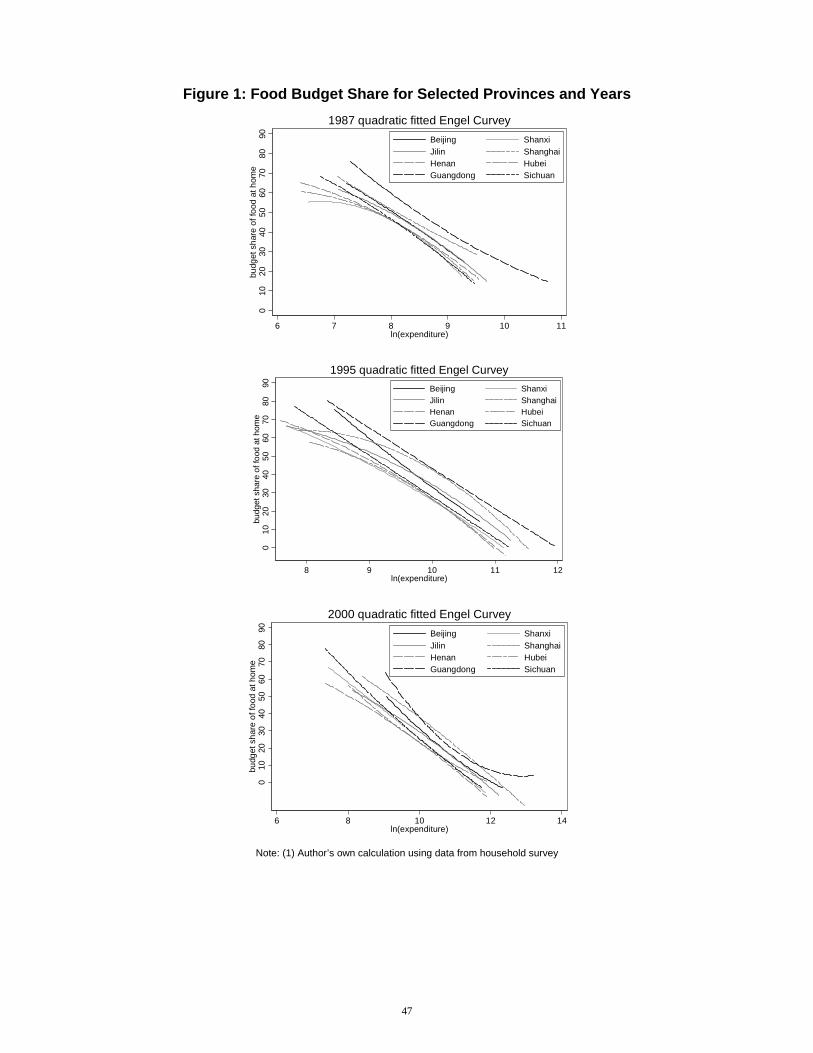
Figure 1: Food Budget Share for Selected Provinces and Years

010

2030

4050

6070

8090

budg

et s

hare

of f

ood

at h

ome

6 7 8 9 10 11ln(expenditure)

Beijing ShanxiJilin ShanghaiHenan HubeiGuangdong Sichuan

1987 quadratic fitted Engel Curvey

010

2030

4050

6070

8090

budg

et s

hare

of f

ood

at h

ome

8 9 10 11 12ln(expenditure)

Beijing ShanxiJilin ShanghaiHenan HubeiGuangdong Sichuan

1995 quadratic fitted Engel Curvey

010

2030

4050

6070

8090

budg

et s

hare

of f

ood

at h

ome

6 8 10 12 14ln(expenditure)

Beijing ShanxiJilin ShanghaiHenan HubeiGuangdong Sichuan

2000 quadratic fitted Engel Curvey

Note: (1) Author’s own calculation using data from household survey

47

Figure 2: Comparison of SPI over time, 1986, 1995, and 2001 Panel A: (Sorted by 1986 SPI)

0.5

11.

5S

patia

l Pric

e In

dex

Gua

ngdo

ngB

eijin

gJi

linS

hang

hai

Liao

ning

Jian

gsu

Qin

ghai

Zhej

iang

Sha

ndon

gTi

enjin

Gua

ngxi

Fujia

nG

ansu

Xinj

iang

Anh

uiH

eilo

ngjia

ngS

ichu

anH

ubei

Gui

zhou

Nin

gxia

Nei

mon

gH

unan

Jian

gxi

Heb

eiYu

nnan

Sha

anxi

Shan

xiH

enan

1986 SPI 1995 SPI2001 SPI

Panel B: (Sorted by 1995 SPI)

0.5

11.

5Sp

atia

l Pric

e In

dex

Gua

ngdo

ngS

hang

hai

Fujia

nB

eijin

gTi

enjin

Gua

ngxi

Liao

ning

Jian

gsu

Xinj

iang

Zhej

iang Jilin

Hei

long

jiang

Qin

ghai

Anhu

iG

ansu

Sic

huan

Jian

gxi

Hub

eiH

unan

Gui

zhou

Nei

mon

gYu

nnan

Heb

eiS

hand

ong

Nin

gxia

Hen

anS

haan

xiSh

anxi

1986 SPI 1995 SPI2001 SPI

Panel C: (Sorted by 2001 SPI)

0.5

11.

5Sp

atia

l Pric

e In

dex

Shan

ghai

Beiji

ngG

uang

dong

Fujia

nQ

ingh

aiTi

enjin

Xinj

iang

Liao

ning Jilin

Hei

long

jiang

Jian

gsu

Zhej

iang

Gan

suA

nhui

Gua

ngxi

Gui

zhou

Nin

gxia

Heb

eiN

eim

ong

Hub

eiS

ichu

anSh

ando

ngJi

angx

iH

unan

Yun

nan

Sha

anxi

Shan

xiH

enan

1986 SPI 1995 SPI2001 SPI

Note: (1) Author’s own calculation.

48

Figure 3: Mean and Standard Deviation of SPI, 1986-2000

Note: (1) Author’s own calculation.

Figure 4: Comparison of Coefficient of Variation of SPI over time obtained from Various Methods

0.00

0.05

0.10

0.15

0.20

0.25

0.30

0.35

0.40

1986 1987 1988 1989 1990 1991 1992 1993 1994 1995 1996 1997 1998 1999 2000 2001

Coe

ffici

ent o

f Var

iatio

n (E

ngel

's C

urve

, Pric

e da

ta, a

nd U

nit V

alue

)

0.00

0.02

0.04

0.06

0.08

0.10

0.12

Coe

ffici

ent o

f Var

iatio

n (B

rand

t and

Hol

z, 2

007)

Engel Curve Basket cost: price data

Basket cost: Unit value Basket cost: B&H

49

Figure 5: Comparison of SPIs obtained from different methods

for various years 1986 1991

0

0.2

0.4

0.6

0.8

1

1.2

1.4

1.6

Guangdong

Beijing

Jilin

Shanghai

Liaoning

Jiangsu

Qinghai

Zhejiang

Shandong

Tianjin

Guangxi

Fujian

Gansu

Xinjiang

Anhui

Heilongjiang

Sichuan

Hubei

Guizhou

Ningxia

Inner Mongolia

Hunan

Jiangxi

Hebei

Yunnan

Shaanxi

Shanxi

Henan

Hainan

Chongqing

Unit valueEngel curveBrandt and Holz

0

0.2

0.4

0.6

0.8

1

1.2

1.4

1.6

Guangdong

Hainan

Heilongjiang

Liaoning

Tianjin

Fujian

Beijing

Guangxi

Xinjiang

Jilin

Qinghai

Zhejiang

Jiangsu

Shandong

Shanghai

Anhui

Inner Mongolia

Ningxia

Jiangxi

Sichuan

Gansu

Guizhou

Hubei

Hebei

Hunan

Henan

Yunnan

Shaanxi

Shanxi

Chongqing

Unit value price data

Engel curve Brandt and Holz

1997 2001

0

0.2

0.4

0.6

0.8

1

1.2

1.4

1.6

Shanghai

Guangdong

Hainan

Beijing

Tianjin

Fujian

Zhejiang

Liaoning

Jilin

Guangxi

Jiangsu

Xinjiang

Anhui

Heilongjiang

Sichuan

Qinghai

Gansu

Chongqing

Hubei

Jiangxi

Guizhou

Shandong

Hunan

Yunnan

Hebei

Henan

Inner Mongolia

Ningxia

Shanxi

Shaanxi

Unit value price data

Engel curve Brandt and Holz

0

0.2

0.4

0.6

0.8

1

1.2

1.4

1.6

Shanghai

Beijing

Guangdong

Fujian

Qinghai

Tianjin

Xinjiang

Hainan

Liaoning

Jilin

Heilongjiang

Jiangsu

Zhejiang

Gansu

Anhui

Guangxi

Guizhou

Ningxia

Hebei

Inner Mongolia

Hubei

Sichuan

Shandong

Chongqing

Jiangxi

Hunan

Yunnan

Shaanxi

Shanxi

Henan

Unit value Engel curve Brandt and Holz

Note: (1) Author’s own calculation

50

Figure 6: Relationship between Provincial Mean Income and SPI Adj. Mean Income

800

1000

1200

1400

1600

inco

me

(Yua

n)

500 1000 1500 2000 2500SPI adj. income (Yuan)

1986198719881989

1000

1500

2000

2500

3000

inco

me

(Yua

n)

1000 2000 3000 4000 5000SPI adj. income (Yuan)

1990199119921993

3000

4000

5000

6000

7000

8000

inco

me

(Yua

n)

2000 4000 6000 8000 10000SPI adj. income (Yuan)

1994199519961997

4000

6000

8000

1000

0in

com

e (Y

uan)

5000 10000 15000SPI adj. income (Yuan)

1998199920002001

Note: (1) Author’s own calculation. Figure 7: Comparison of Gini Coefficients for Unadjusted and SPI Adjusted

Average Provincial Income

0.000

0.020

0.040

0.060

0.080

0.100

0.120

0.140

0.160

0.180

1986 1987 1988 1989 1990 1991 1992 1993 1994 1995 1996 1997 1998 1999 2000 2001

Reg

iona

l Gin

i Coe

ffici

ent

Regional Gini for unadj. Income

Regional Gini for SPI adjusted income

Note: (1) Author’s own calculation.

51

Figure 8: Comparison of Gini Coefficients for Unadjusted and SPI Adjusted Average household Income

0.10

0.15

0.20

0.25

0.30

0.35

1986 1987 1988 1989 1990 1991 1992 1993 1994 1995 1996 1997 1998 1999 2000 2001

Gin

i Coe

ffici

ent

Income SPI adjusted income

52

Appendix A: Price Ratios of the Highest Province to the Lowest Province 1991-1997

Prices Items Unit 1991 1992 1993 1994 1995 1996 1997 p1 Flour Kg 2.33 2.18 2.41 2.29 2.41 2.38 2.56 p2 Rice Kg 4.28 2.31 2.24 1.81 2.09 2.09 2.00 p3 Stick rice Kg 3.24 2.18 1.84 2.24 2.53 1.77 1.80 p4 Noodle Kg 2.28 2.13 2.31 2.14 2.26 2.05 2.12 p5 Bean Kg 4.00 3.02 3.16 2.95 3.39 3.03 2.36 p6 Tofu Kg 1.94 1.80 1.91 2.97 4.32 4.30 4.06 p7 oil Kg 2.37 2.33 2.52 2.21 2.98 3.33 3.19 p8 Pork Kg 1.75 1.70 2.04 1.66 1.55 1.54 1.57 p9 Beef Kg 1.82 1.75 1.74 1.72 1.77 2.02 1.90 p10 Lamb Kg 3.51 3.66 4.02 5.32 3.17 2.95 2.61 p11 Chicken Kg 2.11 2.27 2.57 3.42 3.16 3.29 2.69 p12 Duck Kg 2.52 2.76 2.69 3.79 3.67 3.79 3.70 p13 Egg Kg 1.71 1.67 1.65 1.88 2.10 1.98 2.53 p14 Huanghua fish Kg 13.16 15.50 14.31 8.39 19.03 18.93 12.81 p15 Dai fish Kg 3.34 2.75 3.40 2.02 2.12 2.21 2.21 p16 Li fish Kg 2.50 2.65 2.76 2.14 1.82 1.74 1.90 p17 Lian fish Kg 2.54 2.64 2.38 3.53 6.00 7.04 6.00 p18 Chao fish Kg 2.42 3.24 3.25 6.12 7.75 7.85 7.44 p19 Salt Kg 2.47 2.63 3.54 2.42 4.92 2.72 2.84 p20 Soy Kg 4.43 5.28 6.94 5.28 6.36 7.01 6.90 p21 Vinegar Kg 9.17 9.28 9.21 6.57 5.26 6.97 7.97 p22 White sugar Kg 1.37 1.59 1.87 1.33 1.51 1.33 1.34 p23 Brown sugar Kg 1.45 1.58 1.81 1.46 1.50 1.67 1.72 p24 Cigerrate 1 Box 3.98 4.82 4.48 5.42 5.39 5.57 4.74 p25 Cigerrate 2 Box 6.76 9.18 9.96 8.70 10.60 10.15 9.34 p26 Alcohol Bottle 3.66 5.17 8.64 8.43 5.73 5.75 6.49 p27 Wine Bottle 9.02 8.72 8.56 8.36 6.99 7.57 6.62 p28 Beer Bottle 2.44 2.15 2.49 2.15 2.73 2.92 4.77 p29 Flavour tear Kg 2.30 2.54 2.64 3.29 3.16 3.13 3.41 p30 Green tea Kg 6.61 9.62 5.92 6.45 11.81 11.73 11.43 p31 Jujube Kg 3.64 3.15 3.19 3.24 4.06 3.62 3.92 p32 Walnut Kg 2.59 2.26 6.34 5.73 4.80 3.13 2.75 p33 Peanut Kg 1.61 1.48 2.25 2.20 2.68 2.61 2.10 p34 Cake Kg 2.56 3.13 13.20 12.61 12.49 11.11 10.84 p35 Bascuit Kg 3.09 2.69 3.89 2.79 2.56 2.83 2.87 p36 Fresh milk Bag 10.08 9.58 11.56 12.37 11.63 8.20 9.02 p37 Milk powder Bag 1.74 1.88 2.41 1.88 1.87 11.58 1.80 p38 Meat can Can 1.45 1.65 1.97 3.04 3.93 4.10 5.23 p39 Shirt Piece 1.91 1.98 3.72 4.66 3.56 4.47 4.22 p40 Trousers Piece 6.87 6.97 21.31 5.53 5.10 7.44 10.82 p41 Jacket Piece 5.18 5.61 6.35 5.84 5.28 5.98 6.98 p42 Sweater Piece 1.83 1.78 2.62 2.59 2.48 2.49 2.40 p43 Dress Piece 8.55 7.16 8.20 6.44 4.90 7.95 7.33 p44 Skirt Piece 6.72 5.64 6.43 5.55 5.23 5.99 5.95 p45 Children clothes Set 2.80 3.83 5.64 5.77 5.52 6.34 7.07 p46 White cloth Metre 1.56 1.48 3.63 3.36 4.13 3.36 3.49 p47 Color cloth Metre 1.49 1.50 3.94 1.99 5.41 2.26 1.94 p48 Flower cloth Metre 1.33 1.28 1.53 1.72 2.61 2.61 2.01 p49 Cambric cloth Metre 4.86 7.45 9.13 6.76 7.84 8.17 7.80 p50 Knitting wool Kg 1.43 1.47 1.48 1.60 1.89 1.96 2.37

Note: Author’s own calculation according to the price data in Statistics of Price Survey (1998), edit by Planning Ministry and National Bureau of Statistic of China (NBS).

53

Appendix A (Cont.1) :

Prices Items Unit 1991 1992 1993 1994 1995 1996 1997 p51 Knitting thread Kg 1.38 1.37 1.42 1.98 2.36 1.71 2.11 p52 Cloth shoes Pair 2.37 2.50 2.41 3.06 3.03 2.30 2.76 p53 Leather shoes Pair 3.54 3.78 3.68 3.07 4.19 3.44 3.23 p54 Towel Piece 3.02 2.85 2.64 2.97 2.90 2.51 2.43 p55 Desk unit 3.96 4.35 7.27 4.83 3.81 4.22 4.30 p56 Mattress unit 2.20 2.21 3.94 4.26 3.26 2.83 2.86 p57 Sewing machine unit 1.42 1.40 2.08 1.47 2.05 1.41 1.43 p58 Washing machine unit 3.81 3.63 3.86 3.57 3.18 3.43 4.39 p59 Eletric Fan unit 1.90 1.78 1.96 3.21 3.17 3.44 3.40 p60 Refrigerator 1 unit 1.62 1.74 1.53 1.53 2.37 1.75 1.87 p61 Refrigerator 2 unit 2.58 2.88 2.80 2.71 2.98 1.73 1.74 p62 Rice cooker unit 2.92 1.46 1.66 1.73 1.82 3.25 1.90 p63 Smoke extractor unit 3.32 3.13 3.62 3.51 3.91 3.63 3.76 p64 Air conditioner unit 4.74 4.81 4.70 4.56 5.50 4.86 6.07 p65 Heater unit 3.67 3.65 3.74 3.62 3.44 3.50 3.85 p66 Blanket Piece 3.50 3.74 4.13 3.90 3.65 4.43 4.63 p67 Linen Piece 1.33 1.49 1.72 2.10 2.21 1.60 1.68 p68 Quilt cover Set 8.11 3.34 3.52 2.36 2.70 3.56 2.94 p69 Bed cover Set 4.50 4.23 4.72 5.32 3.48 3.66 4.19 p70 Soap Piece 2.20 2.29 2.24 2.24 2.31 2.38 2.38 p71 Scented soap Piece 4.26 4.26 4.34 2.83 2.84 3.19 3.16 p72 Washing powder bag 2.78 2.07 3.25 3.36 2.89 3.00 3.13 p73 Tooth paste Piece 5.84 5.30 4.74 3.17 19.61 3.46 17.17 p74 Tissue Roll 5.65 4.41 4.49 5.70 5.37 3.93 4.29 p75 Battery Piece 2.39 2.45 2.55 2.19 8.28 2.95 2.48 p76 Dish washing Bottle 1.66 1.39 1.54 16.33 4.49 2.08 1.98 p77 Gold ornaments G 3.21 2.53 1.43 1.43 2.10 1.41 1.39 p78 Thermometer Piece 1.48 1.48 1.36 1.49 1.58 1.66 1.65 p79 Licorice root Kg 3.93 5.28 4.66 3.68 3.69 2.74 3.28 p80 Pistache Kg 3.60 2.06 2.17 2.10 3.52 1.95 2.40 p81 Motorcycle Unit 5.32 5.58 6.91 6.99 6.58 8.61 8.67 p82 Bicycle Unit 1.44 1.49 1.46 1.60 19.21 2.24 1.94 p83 Telephone Unit 11.83 9.92 9.53 8.92 6.22 5.60 2.18 p84 Radio Unit 3.35 6.87 5.75 6.35 3.63 6.26 5.93 p85 Color TV Unit 1.70 1.80 2.95 2.84 3.09 2.63 2.57 p86 Black&white TV Unit 1.70 13.75 1.88 1.66 2.32 1.54 1.71 p87 Recorder Unit 1.76 2.31 3.77 3.95 4.30 4.30 2.96 p88 Camera Unit 3.54 3.57 4.02 3.98 4.63 4.02 4.09 p89 Video player Unit 2.54 2.44 2.79 2.69 2.70 2.45 2.35 p90 Video camera Unit 3.44 3.70 2.36 2.14 2.63 2.28 2.69 p91 Books Piece 2.15 1.63 1.71 1.90 1.55 2.23 1.81 p92 Film Roll 1.21 1.25 1.20 1.29 1.78 1.29 1.28 p93 Tape Piece 2.20 2.16 2.12 2.51 3.03 2.26 2.22 p94 Newspaper Copy 2.29 2.29 3.02 3.17 3.44 3.50 3.08 p95 Brick Piece 12.87 16.60 14.56 13.59 12.22 9.75 17.80

p96 Glass Square metre 1.61 1.64 2.70 2.03 3.05 2.34 2.41

Tradable Goods 3.53 3.71 4.20 3.98 4.51 4.09 4.15 Note: Author’s own calculation according to the price data in Statistics of Price Survey (1998), edit by national Planning Ministry and National

Bureau of Statistic of China (NBS).

54

Appendix A (Cont.2): Price Items Unit 1991 1992 1993 1994 1995 1996 1997

p97 Housing rent Square metre 5.95 10.23 9.43 6.60 6.73 5.00 5.25

p98 Water Tons 4.18 2.40 3.06 3.44 5.94 2.47 2.65

p99 Electricity Cubic metre 3.42 2.28 3.60 4.17 2.91 2.85 2.53

p100 Coal 100 Kg 3.82 3.60 3.51 6.50 10.86 13.47 9.95 p101 Petrol gas Kg 8.55 7.49 5.47 5.28 5.28 5.32 2.81

p102 Coal gas Cubic metre 31.09 24.82 19.82 19.37 16.61 18.06 17.95

p103 Local phone Once 9.08 9.08 9.08 9.19 9.05 6.59 6.23 p104 Local bus One ticket 8.98 8.71 9.36 10.33 9.41 6.58 8.67

p105 Long distance bus Km. person 28.071 28.07 13.64 47.73 42.00 30.81 28.29

p106 Taxi Km 12.18 8.74 5.03 5.33 3.63 3.65 3.65

p107 Hair dressing service Once 4.84 5.20 5.71 5.73 5.37 5.21 4.86

p108 Shower Once 5.78 8.00 8.03 8.32 10.77 13.09 13.09 p109 Movie One ticket 3.36 4.13 4.74 4.70 7.91 5.76 6.86 p110 Tuition Half year 19.92 16.00 15.75 16.81 15.49 8.22 5.49 p111 Child care Month 5.54 5.57 5.42 4.89 6.75 6.45 6.18 p112 Housework Month 8.93 13.83 17.96 11.94 9.83 11.94 14.52 p113 Shoes repair Pair 3.43 3.42 3.54 4.41 3.78 3.57 3.20 p114 Watch repair Piece 2.59 3.60 9.45 7.48 13.28 16.06 15.04 p115 Sewing Set 6.60 7.84 7.17 6.58 16.78 15.56 15.22 p116 Loundry Piece 7.97 9.31 8.52 4.97 5.21 4.83 5.71 p117 Technical repair Once 12.89 12.62 8.01 4.81 8.28 11.71 14.58 p118 Medical registration Once 5.75 3.78 4.69 6.08 6.52 17.78 11.87 p119 An inject Once 3.94 4.56 3.74 3.13 3.64 4.11 5.17 p120 Bed in hospital Bed/night 2.61 2.85 3.52 3.50 6.51 7.42 6.49 Non-tradable goods and services 8.73 8.59 7.84 8.80 9.69 9.44 9.01

Note: Author’s own calculation according to the price data in Statistics of Price Survey (1998), edit by national Planning Ministry and National Bureau of Statistic of China (NBS).

1 The original data is 117.33 here, which is replaced because it is an outlier.

55

Appendix B. Test of Bias in SPI Using CPI as Deflators over Time 1991 1992 1993 1994 1995 1996 1997 Province ASPI ASPI DSPI ASPI DSPI ASPI DSPI ASPI DSPI ASPI DSPI ASPI DSPI Beijing 1.00 1.00 1.00 1.00 1.00 1.00 1.00 1.00 1.00 1.00 1.00 1.00 1.00 Tianjin 1.02 1.05 1.03 1.07 1.04 1.06 1.03 1.01 1.01 1.05 0.96 0.99 0.90 Hebei 0.91 0.89 0.90 0.83 0.86 0.85 0.82 0.80 0.78 0.79 0.72 0.75 0.64 Shanxi 0.99 0.96 0.98 0.92 0.95 0.89 0.93 0.87 0.90 0.84 0.85 0.79 0.79 Inner Mongolia 0.94 0.94 0.93 0.90 0.89 0.89 0.84 0.81 0.80 0.83 0.73 0.78 0.66 Liaoning 1.09 1.07 1.07 1.03 1.03 1.10 1.01 0.97 0.97 0.95 0.91 0.89 0.84 Jilin 1.11 1.14 1.08 1.19 1.01 1.13 0.92 1.05 0.83 1.05 0.72 1.04 0.61 Heilongjiang 1.02 1.02 1.02 1.12 0.98 0.97 0.93 0.91 0.87 0.93 0.78 0.93 0.69 Shanghai 1.14 1.14 1.14 1.24 1.15 1.23 1.16 1.20 1.17 1.19 1.17 1.12 1.13 Jiangsu 1.02 1.01 1.01 1.09 1.00 1.09 0.99 1.05 0.97 1.05 0.94 0.98 0.89 Zhejiang 1.13 1.13 1.12 1.08 1.14 1.12 1.15 1.06 1.16 1.06 1.15 1.00 1.13 Anhui 0.89 0.91 0.88 0.87 0.84 0.98 0.81 0.80 0.78 0.91 0.74 0.85 0.68 Fujian 1.29 1.21 1.27 1.14 1.22 1.09 1.18 1.02 1.13 0.96 1.04 0.91 0.93 Jiangxi 0.90 0.87 0.88 0.83 0.84 0.92 0.81 0.85 0.78 0.83 0.73 0.78 0.67 Shandong 0.90 0.89 0.89 0.82 0.85 0.95 0.81 0.89 0.77 0.90 0.72 0.85 0.67 Henan 0.95 0.92 0.93 0.84 0.85 0.90 0.79 0.90 0.73 0.86 0.66 0.84 0.59 Hubei 0.96 0.95 0.97 0.88 0.97 0.87 0.99 0.84 1.03 0.84 1.07 0.79 1.07 Hunan 0.97 0.97 1.00 1.02 1.02 1.02 1.04 1.02 1.07 0.97 1.05 0.93 1.01 Guangdong 1.26 1.36 1.24 1.30 1.26 1.26 1.23 1.17 1.16 1.06 1.06 1.00 0.93 Guangxi 0.97 0.96 0.94 0.96 0.95 0.99 0.96 0.97 0.98 0.93 0.95 0.86 0.87 Hainan 1.30 1.25 1.29 1.15 1.33 1.19 1.38 1.10 1.35 1.04 1.24 0.96 1.09 Chongqing 1.05 1.11 1.05 0.98 1.03 1.03 1.03 1.01 1.06 1.07 1.06 1.00 1.06 Sichuan 0.92 0.91 0.92 0.77 0.90 0.97 0.91 0.90 0.92 0.90 0.93 0.84 0.93 Guizhou 0.86 0.83 0.85 0.79 0.82 0.87 0.77 0.80 0.74 0.80 0.70 0.73 0.65 Yunnan 0.90 0.90 0.90 0.90 0.91 0.93 0.85 0.88 0.82 0.87 0.77 0.83 0.72 Shaanxi 0.88 0.89 0.89 0.82 0.86 0.83 0.86 0.81 0.86 0.82 0.85 0.79 0.84 Gansu 0.96 0.92 0.94 0.87 0.89 0.92 0.84 0.89 0.80 0.92 0.75 0.80 0.70 Qinghai 0.86 0.84 0.85 0.76 0.80 0.80 0.75 0.75 0.72 0.75 0.68 0.71 0.65 Ningxia 0.94 0.93 0.93 0.85 0.90 0.90 0.87 0.85 0.83 0.83 0.77 0.78 0.69 Xinjiang 1.07 0.98 1.06 0.88 1.01 0.95 0.98 0.77 0.96 0.90 0.93 0.84 0.89 Mean 1.01 1.00 1.00 0.96 0.98 0.99 0.95 0.93 0.93 0.93 0.89 0.88 0.83 Maximum 1.30 1.36 1.29 1.30 1.33 1.26 1.38 1.20 1.35 1.19 1.24 1.12 1.13 Minimum 0.86 0.83 0.85 0.76 0.80 0.80 0.75 0.75 0.72 0.75 0.66 0.71 0.59 Ratio of max. to min. 1.51 1.64 1.52 1.71 1.66 1.58 1.84 1.60 1.88 1.59 1.88 1.58 1.92 SD 0.12 0.13 0.12 0.15 0.13 0.12 0.15 0.12 0.16 0.11 0.17 0.10 0.17 CV 0.12 0.13 0.12 0.15 0.14 0.12 0.16 0.13 0.17 0.11 0.19 0.12 0.21 Correlation coefficients 0.96 0.86 0.83 0.78 0.71 0.60 Note: ASPI is calculated by basket cost method using prices for each year separately, DSPI is calculated using official provincial CPI as deflators based on ASPI in 1991.

56

Appendix C: Assumption on Food and Non-food Price Bias

In the estimated model, the aggregated unit values of food and non-food are

used to proxy true prices of food and non food. Unit values may over/under value the

true prices

j,fj,fj,f ElnPlnln +=Π , where 0Eln j,f > (1)

j,nj,nj,n ElnPlnln +=Π , where 0Eln j,n > (2)

The estimated general price level is:

))ElnE(ln

exp(p j,nj,fjj β

γφ−

−+= (3)

An important assumption is made to derive SPI, which is that the aggregated

unit values of food and non food have same level of bias at each province:

0)ElnE(ln j,nj,f =− (4)

Under this assumption, the estimated true price

)exp(p jj β

φ−

= where 0>− β (5)

If this assumption is violated, j,nj,f ElnkEln = , where 1≠k , equation (3)

becomes:

))Eln)1k(

exp(p j,njBj β

γφ−−+

= (6)

If unit values of food have higher bias than non-food, 01>−k and 0>γ ,

)exp(P))Eln)1k(

exp(P jj

j,njBj β

φβ

γφ−

=>−−+

= (7)

Then the true price will be under estimated by equation (5).

If unit values of food have higher bias than non-food, 01>−k and 0<γ ,

gives

)exp(P))Eln)1k(

exp(P jj

j,njBj β

φβ

γφ−

=<−−+

= (8)

Then the true price will be over estimated by equation (5).

57