Regime-Switching Stochastic Volatility and Short-Term Interest Rates

Madhu Kalimipalli ♣ School of Business and Economics

Wilfrid Laurier University Waterloo, Ontario N2L 3C5 Tel: 519-884-0710 Ext.: 2187

Mkalimip@wlu.ca

and

Raul Susmel C.T. Bauer College of Business

University of Houston, Houston,Tx-77204-6282, USA rsusmel@uh.edu

(Version: May 2001)

Abstract

In this paper, we introduce regime-switching in a two-factor stochastic volatility model to explain the behavior of short-term interest rates. The regime-switching stochastic volatility (RSV) process for interest rates is able to capture all possible exogenous shocks that could be either discrete, as occurring from possible changes in the underlying regime, or continuous in the form of `market-news' events. We estimate the model using a Gibbs Sampling based Markov Chain Monte Carlo algorithm that is robust to complex non-linearities in the likelihood function. We compare the performance of our RSV model with the performance of other GARCH and stochastic volatility two-factor models. We evaluate all models with several in-sample and out-of-sample measures. Overall, our results show a superior performance of the RSV two-factor model. Key Words: Short-term interest rates, stochastic volatility, regime switching, MCMC methods. JEL Classification: G12

♣ We acknowledge the comments of Arthur Warga, and seminar participants at the University of Houston, McGill University and the NFA 2000 Meetings in Waterloo. We thank Siddhartha Chib for providing us with very helpful computational tips.

2

Regime -Switching Stochastic Volatility and Short-Term Interest Rates In this paper, we introduce regime-switching in a two-factor stochastic volatility model to explain the behavior of short-term interest rates. The regime-switching stochastic volatility (RSV) process for interest rates is able to capture all possible exogenous shocks that could be either discrete, as occurring from possible changes in the underlying regime, or continuous in the form of `market-news' events. We estimate the model using a Gibbs Sampling based Markov Chain Monte Carlo algorithm that is robust to complex non-linearities in the likelihood function. We compare the performance of our RSV model with the performance of other GARCH and stochastic volatility two-factor models. We evaluate all models with several in-sample and out-of-sample measures. Overall, our results show a superior performance of the RSV two-factor model. Key Words: Short-term interest rates, stochastic volatility, regime switching, MCMC methods. JEL Classification: G12

3

I. Introduction

The volatility of short-term interest rates plays a crucial role in many popular two-

factor models of the term structure. The level and the volatility of the short rate are

commonly used as state variables in two-factor models. For example, Longstaff and

Schwartz (1992) derive a two-factor general equilibrium model, with the short rate’s level

and the short rate’s conditional volatility as factors. They show that a two-factor model

improves upon a single factor model, which only uses the level of the short rate. They find

that the conditional volatility factor provides additional information about the term

structure that may be useful in pricing interest rate options and hedging interest rate risk.

Similarly, Brenner et al. (1996) include a level effect and a GARCH effect into their

interest rate model. They find that models with both level and GARCH effects outperform

those that exclude one of them. Note that a GARCH model displays a single continuous

information shock; while in a stochastic volatility (SV) model there are two continuous

information shocks. Following this more general formulation for the conditional variance,

Anderson and Lund (1997) and Ball and Torous (1999) include a level factor and a

stochastic volatility factor into the interest rate mean specification. They find a two-factor

model with stochastic volatility performs better than the more traditional two-factor model

with GARCH volatility. The information shocks in both GARCH and SV models are

continuous. Ball and Torous (1995) build a two-factor model, but introducing discrete

shocks from an underlying state variable that follows a two-state Markov process. In Ball

and Torous (1995), the conditional volatility displays Hamilton’s (1989) regime-

switching.

Introducing regime-switching in the volatility process of the short-term interest

rate is consistent with previous studies that document a strong evidence for regime-

switching in short-term interest rates (see Hamilton (1988), Driffill (1992) and Gray

(1996)). Regime-switching in the volatility process of the short rate has important

implications for the dynamics of the yield curve and immunization strategies. As

pointed out by Litterman, Scheinkman and Weiss (1991), the volatility of the short rate

(for example, three-month T-Bill rate) affects the curvature of yield curve1. In

1 See also Brown and Schaefer (1995).

4

particular, the volatility of the short rate has two counteracting effects on the yield

curve. First, higher volatility of the short rate induces higher expected rates for the

longer maturities (premium effect). Second, higher volatility of the short-term interest

rate increases the convexity of the discount factor function and, therefore, reduces the

yields for longer maturities (convexity effect). The premium effect dominates at the

short end of the yield curve, while the convexity effect dominates at the long end

making the yield curve more humped. When regime switching is not considered,

volatility shocks tend to be very persistent and, therefore, the convexity effect and the

hump in the yield curve could be more pronounced than they ought to be. Gray (1996)

notes that there is evidence for 1) mean reverting high-volatility state with low

volatility persistence, and 2) non-mean reverting low-volatility state with high volatility

persistence in one-month U.S. T-Bill yields. This implies that the shape of the yield

curve depends upon the dynamics of the short rate, its volatility and the latent volatility

state.

Regime-switching in the volatility process also has important implications for

hedging. A trader should account for both continuous and discrete shocks to volatility

in computing dynamic hedge ratios. While continuous shocks refer to market-news

events, discrete shocks could refer to the high or low volatility states of the market,

high or low liquidity in the market or high or low sentiment in the market.

In this paper, we follow Ball and Torous (1995) and Anderson and Lund (1997).

We introduce regime-switching in a two-factor model, where volatility follows a SV

process. We model the volatility of short-term interest rates as a stochastic process whose

mean is subject to shifts in regime. That is, our switching stochastic volatility for interest

rates captures all possible exogenous shocks that could be either discrete, as occurring

from possible changes in underlying regime, or continuous, in the form of “market news”

events. We estimate our two-factor regime-switching stochastic volatility model for short-

term interest rates using a Gibbs Sampling based Markov Chain Monte Carlo algorithm.

We conduct an extensive in-sample and out-of-sample evaluation of our two-factor model

against other two-factor models. In-sample, our model performs substantially better than

the GARCH based two-factor models and the single-state stochastic volatility two-factor

models. Out-of-sample, the regime-switching stochastic volatility model tends to

5

outperform the other models. The out-of-sample forecasts from the regime-switching

stochastic volatility model, however, are not that different from the single-state stochastic

volatility model.

The rest of the paper is structured as follows. Section II introduces our regime-

switching stochastic volatility (RSV) two-factor model. Section III examines the data set

used in this paper. Section IV discusses the results from estimation. Section V presents the

in-sample and out-of-sample comparative performance of the RSV model. Section VI

summarizes and presents our conclusions.

II. Two-Factor Models and Regime Switching

A common empirical finding in two-factor models is the high persistence in the

conditional variance. For example, Brenner et al. (1996) estimate the persistence

parameter in the conditional variance equation to be 0.82 using weekly three-month U.S.

T-Bill data. Ball and Torous (1999) report persistence parameter to be 0.928 using

monthly one-month U.S. T-Bill data, while Anderson and Lund (1997) report volatility

persistence to be 0.98 for weekly three-month U.S. T-Bill data.

High persistence in the conditional variance implies that shocks to the conditional

variance do not die out quickly -i.e., current information has a significant effect on the

conditional variance for future horizons. Lamoreux and Lastrapes (1990) show that high

persistence could be related to possible structural changes that have occurred during the

sample period in the variance process. They find that a single-regime GARCH

specification leads to spurious high persistence under the presence of structural breaks. By

allowing for possible regime switching in the data, high persistence observed in the single

regime models seems no longer valid. Similar results have been documented by Hamilton

and Susmel (1994), Cai (1994) and So, Lam and Li (1998).

Hamilton (1988) and Driffill (1992), among others, find strong evidence for

regime-switching in the U.S. short-term interest rates. Various macro-economic events

were responsible for regime switching in the U.S. interest rates. These events include

the OPEC oil crisis, the Federal Reserve experiment of 1979-82, the October 1987

crash and wars involving U.S. and rest of the world. When short rates could switch

randomly between different regimes –i.e., where each regime is associated with its own

6

mean and variance-, we may find high persistence in the data when we average data

from different regimes. It is the possibility of a shift in the underlying regime that we

explicitly incorporate in our short-rate process. Next, we introduce a two-factor model

that nests level and stochastic volatility effects.

Consider the short-term interest rate process described below:

In model (1), rt is the short rate and ht is the conditional variance of the short rate, α

captures the levels effect in the model, µ is the stationary mean of the log conditional, φ1

measures the degree of persistence of conditional variance, and ε t and ηt represent shocks

to the mean and to the volatility, respectively. Both shocks are white noise errors, which

are assumed to be distributed independently of each other. We call model (1) the Single-

state Stochastic Volatility (SSV) model. This model is used in Ball and Torous (1999) and

in Anderson and Lund (1997). The estimation of SSV models involves the estimation of

mean parameters α0, α1 and variance parameters α, β , ση, φ1. Note that model (1)

with a GARCH specification instead of a SV specification for the conditional volatility

becomes the Brenner et al. (1996) model.

Now, let µ be a function of the latent state st, which follows a k-state ergodic

discrete first-order Markov process as in Hamilton (1988). That is, at a given point in

time, the mean of the log volatility belongs to one of the k states. A k-state stationary

transition probability matrix governs the dynamics of the transition from one state to the

next state. This implies that the latent volatility, ht, is driven by a continuous shock, ηt, as

in (1) above and also by a discrete shock st that takes on discrete integer values 1, 2, ...,

k. We can also think of our latent volatility as a mixture of k densities, where each

density corresponds to a single state. The latent volatility at a given time comes from a

single density, which is decided by an underlying k-state Markov process. That is, our

Regime-switching Stochastic Volatility (RSV) model is given by:

( ) ( )(1) '

)ln()ln

0 ,

12

11

211101

βµ

ησµφµ

αεαα

η

α

t

ttt

tttttt

x

h(h

rhrrr

=

+−=−

>++=−

−−

−−−

( ) ( )

(2) 21 0

)ln()ln

5.0 ,

12

11

211101

1

,...k,ss

h(h

rhrrr

tts

tstst

tttttt

t

tt

=>+=

+−=−

=++=−

−−

−−−

−

γγβµ

ησµφµ

αεαα

η

α

7

where µs(t) refers to the state dependent mean of conditional volatility. The parameter γ

measures the sensitivity of the mean with respect to the underlying state and is constrained

to be positive. The underlying state st can assume k possible states, i.e. one of 1,2, .....,k

where higher values of st lead to higher intercept terms in the log variance equation. As an

identification condition, we require each regime to correspond to at least one time point.

In addition, and mainly for convenience, we set the level parameter α=0.5, which has been

used in many previous papers.2 This assumption also avoids potential non-stationary

problems associated with α > 1, as shown in Gray (1996) and Bliss and Smith (1998). The

estimation of the RSV model involves estimation of mean parameters α0, α1, variance

parameters β , γ, ση, φ1, and the transition probability parameters p01, p10, where pij

represents the transition probability of going from state i to j.

In summary, the RSV model specification combines a level effect and a

conditional volatility process that captures all possible exogenous shocks. Note that the

RSV model reduces to the SSV model when there is no regime shift in the data -i.e., when

γ is restricted to zero.

A closely related paper is So, Lam and Li (1998), which uses a switching

stochastic volatility model to explain the persistence in the log volatility for S&P 500

index weekly returns. Using a three-state model (with high, medium and low volatility

states), So et al. (1998) find that the volatility state is less persistent, while the low

volatility state is more persistent. Our model slightly differs from So et al. (1998). In our

RSV model, the drift term of the conditional variance is a function of both current and last

period states, while in So et al. (1998) the conditional variance is a function only of the

current period state. This difference in our volatility specifications also leads to

differences in our likelihood functions and, hence, in our posterior densities.

Estimation of the RSV model involves estimating two latent variables -i.e., ht and

st in addition to the model parameters. In the presence of two latent variables, the

likelihood function for the model needs to be integrated over all the possible states of the

two latent variables. Jacquier, Polson and Rossi (1993) show that maximum likelihood

based methods tend to fail under complex specifications of the likelihood function.

Consequently, we resort to Monte Carlo Markov Chain (MCMC) methods to estimate the

2 For example, Cox, Ingersol and Ross (1985) and Anderson and Lund (1997).

8

RSV model.3 Note that Model 3 can easily incorporate more complicated dynamics. For

example, we can make ση a function of a latent state, or we can specify an ARMA

structure for the conditional mean equation (with parameters driven by the latent state), or

we can consider multiple regimes. Our estimation technique can accommodate all these

extensions.

III. Data

The data consists of annualized yields based on weekly observations of three-

month U.S. T-bill data for the period 01/06/60 to 06/03/98 (2003 weekly observations)

and is obtained from the Chicago Federal Reserve’s database. Wednesday’s rates are used

and if Wednesday is a trading holiday, then, Tuesday's rates are used. Similar data sets

have been previously used by Anderson and Lund (1997) and Gray (1996).

Figure 1 plots the annualized yields and also the first differences in yields based on

weekly observations of three-month T-Bill data. There are several episodes of large

fluctuations in nominal interest rates: the oil shocks during 1969-71 and 1973-75, the

Federal Reserve monetary experiment of 1978-82, and the market crash of 1987. This

observation suggests more than a single regime in the data. For instance, we can think of a

high volatility regime during the periods cited above and a low volatility regime during

rest of the periods. We could allow for an additional regime, as in Hamilton and Susmel

(1994), to capture outliers in the data. Following the existing switching literature,

however, we limit ourselves to two regimes for the underlying volatility.

The weekly three-month T-Bill rate (rt) is non-stationary4. First differencing makes

the data stationary. Using Box-Jenkins methods, an ARIMA(1,1,0) model seems to

provide a satisfactory fit for the autocorrelations in the yields. Following Pagan and

Schwert (1990) and Ball and Torous (1995, 1999), we fit the RSV model (2) to the

residuals (RESt) from regressing ∆rt on a constant and ∆rt-1. For the purpose of estimation

and comparison to alternative volatility models, we write our mean adjusted version of the

RSV model as

3 Appendix A gives the details of our MCMC estimation and Appendix B presents the results of a simulation experiment using our estimation method. 4 ADF tests could not reject the null of a unit root in the yield series.

9

where all the assumptions on the error terms made in (2) still hold. Again, note that when

we set γ to zero, the RSV model reduces to the SSV model.

Table 1 presents the summary statistics of the data. Changes in yields, ∆rt, seem to

be left skewed indicating that periods of high T-Bill returns were less common compared

to periods with low returns. There is also a strong evidence of kurtosis in the return series.

The Ljung-Box statistic suggests that there is a high degree of autocorrelation for the raw

yields (rt). There is a very high persistence in the raw series. On the other hand, ∆rt series

seems to be much less persistent and is characterized by low autocorrelations. High

autocorrelation in the two series (∆rt)2 and log(∆rt)2 suggests the kind of non-linearity in

the data that can be explained by a SV model. Table 2 presents the results from GARCH

tests on the data. We report the Ljung-Box statistic for the squared residuals (RESt2) at

various lags. The null of no GARCH effects is strongly rejected by the data.

IV. Results from the Stochastic Volatility models

To benchmark our results, first, we ignore the possibility of regime-switching in

the data. The results from the MCMC estimation of the SSV model are presented in Table

3, where the parameter set is θ = β , φ, ση. The persistence parameter φ is very high

indicating that the half-life of a volatility shock, measured as -ln(2)/ln(φ), is about fourteen

weeks. Standard errors for the parameters are small indicating that parameters are highly

significant. Figure 2 plots the posterior densities of the parameters. All the parameters

have symmetric densities while half-life density is right skewed indicating that half-lives

longer than fourteen weeks are more common.

We, next, estimate the RSV model for our weekly interest data set. Table 5

presents the prior and posterior parameter estimates of the parameter set θ in our model,

where θ = β , γ, φ, σ η, p01, p10. Standard errors for the parameters are small as before.

( ) ( ) (3) 21 0

)ln()ln

5.0 ,

)ˆˆ(

12

11

21

110

1

, ss

h(h

rhRES

RESrr

tts

tstst

tttt

ttt

t

tt

=>+=

+−=−

==

≡∆+−∆

−−

−

−

−

γγβµ

ησµφµ

αε

αα

η

α

10

The persistence parameter, φ, drops significantly to 0.628 from 0.951 in the SSV model.

This implies that a switch in the latent regime creates a high persistence in volatility and

confirms the earlier results of Hamilton and Susmel (1994), Cai (1994) and So, Lam and

Li (1998). The distribution of φ is left skewed with a median 0.647 (see Figure 3),

implying that even lower persistence than 0.628 is common. The transition probabilities,

p00 and p11, are estimated as 0.994 and 0.966. These estimates are comparable to 0.9896

and 0.9739 respectively reported in Gray (1996) and 0.9878 and 0.9402 respectively

reported in Cai (1994). Our results imply that the effect of a volatility shock is much more

persistent in the low volatility state than in the high volatility state. A volatility shock lasts

on average of, at least, 100 weeks in the low volatility state compared to about 30 weeks

in the high volatility state, where duration of the shock is obtained as (1-pii)-1. Figure 3

plots the Gaussian kernel densities for the posterior parameter estimates. The posterior

densities seem to be symmetric for β and γ and right skewed for σ η (with a median 0.897).

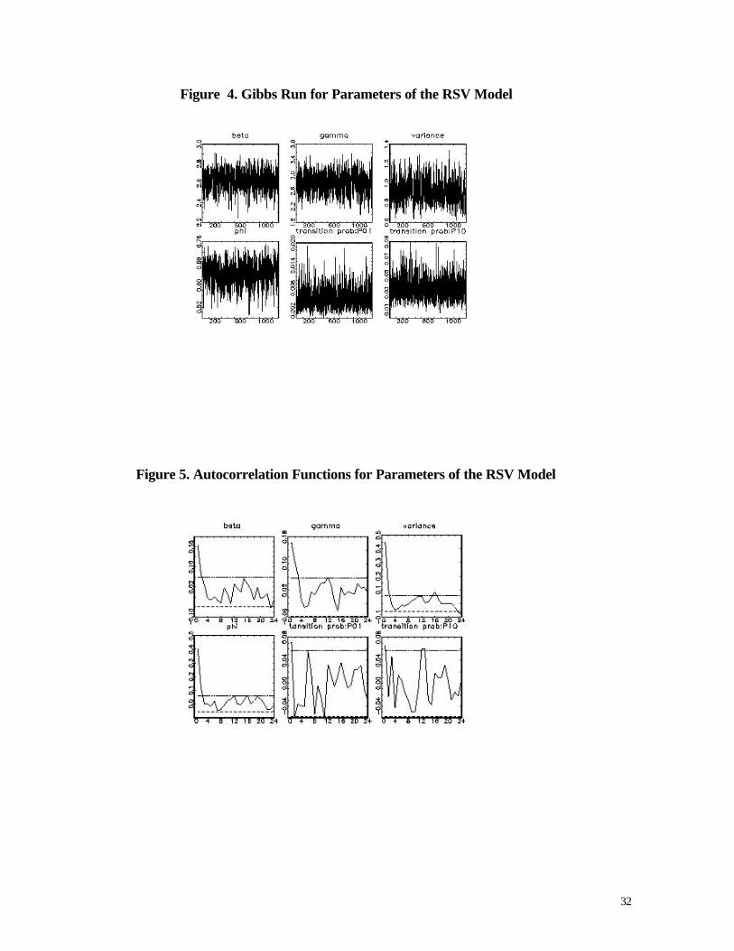
Figure 4 plots the Gibbs parameter estimates from 1200 runs (details in appendix A).

Gibbs runs indicate no autocorrealtion in successive draws. Figure 5 plots autocorrelations

for the parameters. The autocorrelations become insignificant at very early lags implying

that the Gibbs draws are drawn at random.

Tables 4 and 6 present the correlations between the parameters. Both Tables 4 and

6 report strong negative correlation between β and φ, and φ and ση. Table 6 also reports

strong positive correlations between β and γ, and β and σ η. Together, these results imply

that 1) as the variance persistence decreases the unconditional variance -i.e., the long-run

mean of ln(ht)- increases, 2) large volatility shocks are not as persistent as small volatility

shocks and 3) large volatility shocks tend to be associated with higher long-run mean

compared to small volatility shocks.

The first two panels of Figure 6 plot the T-Bill yields and the residuals from a

regression of ∆rt on a constant and ∆rt-1, respectively. The third panel plots the underlying

annualized volatility (generated by a multi-move simulation smoother), and the fourth

panel plots the simulated smoother probabilities of being in high volatility state, i.e.,

Prob(st =1). Following Hamilton (1988), we consider an observation as belonging to state

one if the smoothed probability is higher than 0.5. The simulation smoother shows periods

of high volatility during the oil shocks of 1969 and 1973, the 1979-83 Federal Reserve

11

monetary experiment, and the market crash of 1987. The smoother probabilities indicate

that there is a large probability that the T-Bill yields during 1969, 1973, 1979-82, and

1987-88 belong to a high volatility regime. This dating is in agreement with the dating

reported by Cai (1994) and Gray (1996).

V. Performance of the RSV Model

We conduct an extensive evaluation of the in-sample and out-of-sample

performance of the SV two-factor models and other two-factor models, based on the

GARCH family of models. We consider three popular GARCH models: GARCH(1,1)

model, GARCH(1,1)-L model -i.e., GARCH(1,1) with an asymmetry effect of negative

lagged errors, to capture the leverage effect- and EGARCH(1,1) model. The first GARCH

model is the formulation used by Longstaff and Schwartz (1992). The second and third

GARCH models retain a leverage effect, as in Brenner et al. (1996). All the GARCH

models are specified to include a level effect (for specifications see Table 7). The MLE

results for the three GARCH models are presented in Table 7. There is evidence for a

leverage effect based on the significant t-statistic for κ in the GARCH(1,1)-L model and

the significant t-statistic for δ2 in the EGARCH(1,1) model. The leverage effect, however,

is small relative to the usual size found in equity returns. All the estimates in the

conditional variance equation are significant for the three models. Note that the estimates

show the usual high persistence in the conditional variance.

We extract one-week(step)-ahead in-sample forecast variances from the single

state and regime-switching two-factor models and compare them to other models. In

addition to the full sample period, 01/06/60-06/03/98, we consider three sub-sample

periods. The three sub-sample periods are: (1) 01/06/60-31/12/78, (2) 01/06/60-31/12/82,

and (3) 01/06/60-31/12/91. The first sample includes the oil shocks, the second sample

includes the Fed monetarist experiment of 1979-82, and the third sample includes the

October1987 stock market crash. Based on the estimates for the three sub-samples, we

estimate out-of-sample forecasts until the end of the sample. We also consider shorter

samples and shorter out-of-sample forecast periods. As an example, we include a fourth

sample 01/01/76-31/12/87, which allows an evaluation of the performance of the model in

12

a shorter data set. This forth sample has two well defined spells of high volatility: the Fed

experiment and the October 1987 stock market crash.

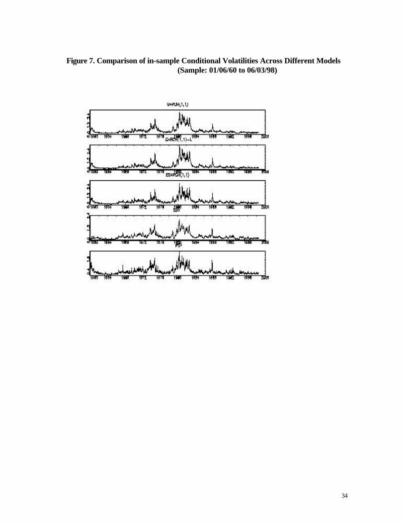
Figures 7 and 8 show the in-sample (annualized) conditional volatilities implied by

all the models. The conditional volatilities from two-factor models are relatively less

smooth compared to those from the GARCH type models. This is because the two-factor

models are more sensitive to shocks. For example, the RSV two-factor model picks up an

outlier in late 1982, which goes undetected by the other models.

Table 8 shows the likelihood function for all the models. The RSV has the biggest

likelihood. Unfortunately, the GARCH models and the SSV models are not nested.

Therefore, standard likelihood ratio tests are not correct. In addition, standard likelihood

ratios cannot be used for the SSV model and the RSV model since there are unidentified

parameters under the null hypothesis of no-switching -see Hansen (1992). Therefore,

Table 8 shows four different in-sample evaluation criteria for the different models. The

stochastic volatility models perform better than all the GARCH models and the SSV

model. In particular, the RSV model has a higher likelihood function, higher adjusted R2,

and higher AIC/SBC values relative to the GARCH models and the SV model. Table 8

also reports posterior odds ratios of the competing model with respect to the constant

variance model –see Kim and Kon (1994). If the odds ratio is positive, then the competing

model is “more likely” to have generated the data than the constant variance model. The

model with the highest value of posterior odds ratio represents the “most likely”

competing model specification. The stochastic volatility models have higher odds ratios

than GARCH models. In particular, the RSV model has an odds ratio at least 56% higher

than the other competing models. Among the two-factor GARCH models, with the

exception of the Adjusted R2 criteria, the E-GARCH(1,1) performs better than the other

models for all the evaluation measures. The E-GARCH(1,1) is also the model used by Ball

and Torous (1999) to evaluate the in-sample evaluation of the SSV model. Based on these

considerations, the E-GARCH(1,1) is the GARCH model we select to evaluate the out-of-

sample performance of the SV models.

Table 9 presents in-sample and out-of-sample one-step ahead forecasts for all the

models for the four different sub-samples. We present the mean squared errors (MSE) and

mean absolute errors (MAE) for the SSV model, the RSV model, a constant volatility

13

model, and for the best performing GARCH model, the E-GARCH(1,1). We keep a

constant volatility model in our out-of-sample comparison, given the results in Figlewski

(1997), where the constant volatility performs well relative to GARCH models. Table 9

shows that the RSV model tends to outperform the GARCH and SSV models. Consistent

with the in-sample results of Table 8, the RSV model always beats in-sample the other

formulations. Out-of-sample, the RSV tends to do better than the EGARCH and SSV

model. The out-of-sample performance of the RSV model, however, is similar to the out-

of-sample performance of the SSV model. Consistent with Figlewski (1997), the constant

variance model shows a good out-of-sample performance, especially in the MSE metric.

Note that the constant variance model in the first sub-sample beats all the other models.

The E-GARCH model never performs better than the SV models. The last sub-sample

presents a short period of out-of-sample forecasts, only one year. Again, the RSV model is

the dominating model.5

VI. Conclusions

In this paper, we introduce regime-switching in a stochastic volatility model to

explain the behavior of short-term interest rates. The regime-switching stochastic

volatility process for interest rates captures all possible exogenous shocks that are

either continuous in the form of `market-news' events or discrete as occurring from

possible changes in underlying regime. We introduce the regime-switching stochastic

volatility process in a two-factor model for the short-term interest rate. We estimate the

two-factor model using a Gibbs Sampling based Markov Chain Monte Carlo algorithm

that is robust to the usual non-linearities in the likelihood function. We find that the

usual high volatility persistence is substantially reduced by the introduction of regime-

switching. We conduct an extensive in-sample and out-of-sample evaluation of several

two-factor models. We use several sub-samples and different evaluation criteria to

compare the RSV model with other GARCH models and single-state stochastic

volatility model. Overall, our results are very supportive of our RSV two-factor model.

5 For the fourth sample, we also calculate (not reported) out-of-sample forecasts for a two-year period and a ten-year period. Overall, the results are similar, although as the out-of-sample forecasting period is extended, the performance of the SSV model becomes very similar to the performance of the RSV model.

14

In-sample and out-of-sample, the RSV model tends to outperform all the other two-

factor models.

15

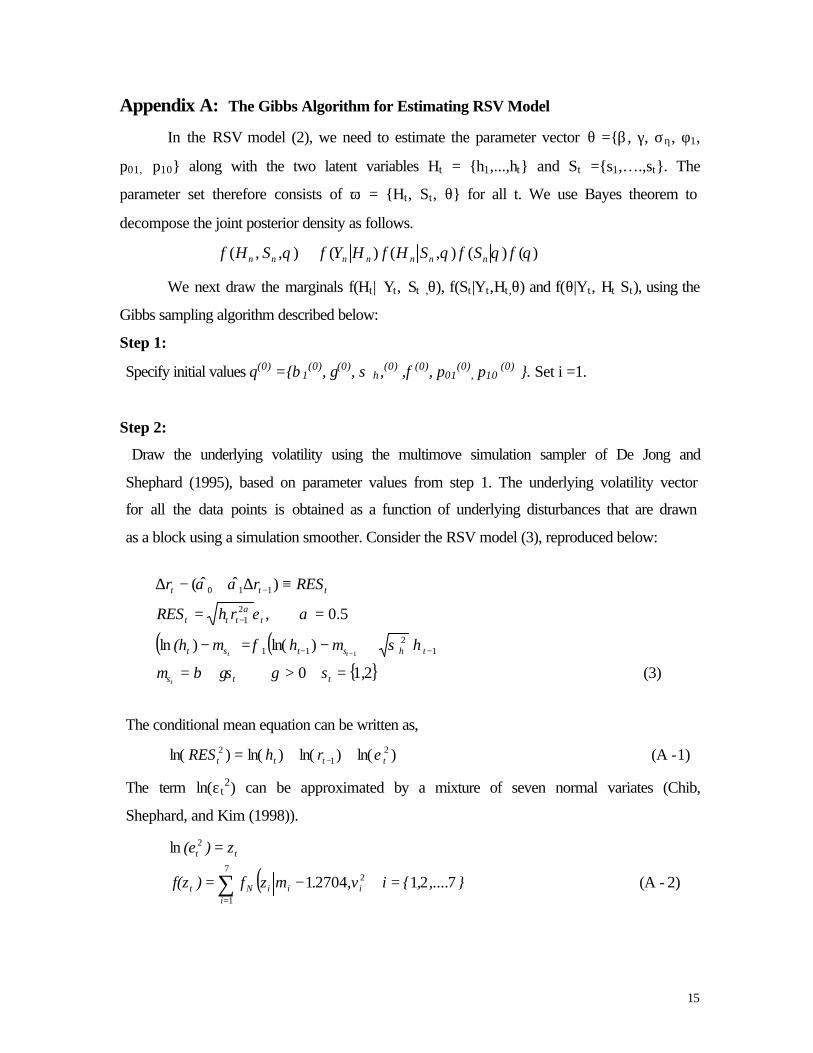
Appendix A: The Gibbs Algorithm for Estimating RSV Model

In the RSV model (2), we need to estimate the parameter vector θ =β , γ, ση, φ1,

p01, p10 along with the two latent variables Ht = h1,...,ht and St =s1,….,st. The

parameter set therefore consists of ω = Ht, St, θ for all t. We use Bayes theorem to

decompose the joint posterior density as follows.

)()(),()(),,( θθθθ fSfSHfHYfSHf nnnnnnn ∝

We next draw the marginals f(Ht| Yt, St ,θ), f(St|Yt,Ht ,θ) and f(θ|Yt, Ht St), using the

Gibbs sampling algorithm described below:

Step 1:

Specify initial values θ(0) =β1(0), γ(0), σ η,(0) ,φ(0), p01

(0), p10

(0) . Set i =1.

Step 2:

Draw the underlying volatility using the multimove simulation sampler of De Jong and

Shephard (1995), based on parameter values from step 1. The underlying volatility vector

for all the data points is obtained as a function of underlying disturbances that are drawn

as a block using a simulation smoother. Consider the RSV model (3), reproduced below:

The conditional mean equation can be written as,

1)-(A )ln()ln()ln()ln( 21

2tttt rhRES ε++= −

The term ln(ε t2) can be approximated by a mixture of seven normal variates (Chib,

Shephard, and Kim (1998)).

( ) 2)-(A 72127041

ln7

1

2

2

,...., i,v.mzf)f(z

z)(e

iiiiNt

tt

=−=

=

∑=

( ) ( ) (3) 21 0

)ln()ln

5.0 ,

)ˆˆ(

12

11

21

110

1

, ss

h(h

rhRES

RESrr

tts

tstst

tttt

ttt

t

tt

=>+=

+−=−

==

≡∆+−∆

−−

−

−

−

γγβµ

ησµφµ

αε

αα

η

α

16

Now, (A-1) can be written as

[ ] 3)-(A )ln()ln()ln( 12 ikzrhRES ttttt =++= −

where kt is one of the seven underlying densities that generates zt. Once the underlying

densities kt, for all t, are known, (A-3) becomes a deterministic linear equation and along

with the RSV model (3) can be represented in a linear state space model. Next, apply the

De Jong and Shephard (1995) simulation smoother to extract the underlying log volatility

from the observed data.

Step 3:

Based the on output from steps 1 and 2, the underlying kt in (A-3) is sampled from

normal distribution as follows -see Chib, Shephard and Kim (1998):

[ ] ( ) 4)-(A k i ,2704.1)ln()ln(),ln( 22 ≤−+∝= iitiNittit vmhzfqhyzf

For every observation t, we draw the normal density from each of the seven normal

distributions kt = 1,2,..,7. Then, we select a “k” based on draws from uniform

distribution.

Step 4:

Based on the output from steps 1, 2 and 3, we draw the underlying Markov-state

following Carter and Kohn (1994). We use the smoother for the above state-space model

(3), to derive the vector of underlying state variable st, t = 1,2,...,n

Step 5:

Cycle through the conditionals of parameter vector θ =β , γ, ση, φ1, p01, p10 for the

volatility equation using Chib (1993), using output from steps 1-4. Assuming that f (θ) can

be decomposed as:

5)-(A ),,,,(),,,(

),,,(),,,(),,,(),,(

1001

22

ijpnnnnnn

nnnnnnnnnnnn

SHYppfSHYf

SHYfSHYfSHYfSHYf

−−

−−−∝

θθφ

θσθγθβθ

φ

σγβ

where θ-j refers to the θ parameters excluding the jth parameter. The respective

conditional distributions (normal for β , γ and φ, inverse gamma for σ2 and beta for pij) are

17

described in Chib (1993). The parameter γ is drawn using an inverse CDF with the

restriction that it is positive. The prior means and standard deviations are specified in

Tables 3 and 5.

Step 6: Go to step 2.

Estimation of SSV model (2) has the same steps as in RSV model (3), except that we do

not have to draw the latent states and transition probabilities. For the Gibbs estimation, we

leave out the first 4000 draws (i.e., burn–in iterations are 4000) and sample from the next

6000 draws. We choose every fifth observation to minimize, and if possible eliminate, any

possible correlation in the draws. Our effective number of draws therefore drops to 1200

(i.e., effective test iterations are 1200). We construct 95% confidence intervals for the

parameters, based on 1200 draws. We construct the standard errors for the parameters

using the batch-means method -see Chib (1993). We estimate the density functions for the

parameters using the Gaussian kernel estimator -see Silverman (1986).

18

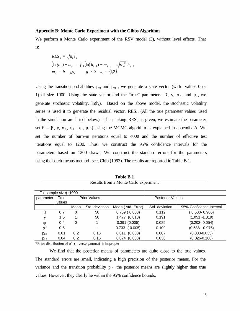
Appendix B: Monte Carlo Experiment with the Gibbs Algorithm

We perform a Monte Carlo experiment of the RSV model (3), without level effects. That

is:

Using the transition probabilities p01 and p01 , we generate a state vector (with values 0 or

1) of size 1000. Using the state vector and the “true” parameters β , γ, ση, and φ1, we

generate stochastic volatility, ln(ht). Based on the above model, the stochastic volatility

series is used it to generate the residual vector, RESt. (All the true parameter values used

in the simulation are listed below.) Then, taking RESt as given, we estimate the parameter

set θ =β , γ, ση, φ1, p01, p10 using the MCMC algorithm as explained in appendix A. We

set the number of burn–in iterations equal to 4000 and the number of effective test

iterations equal to 1200. Thus, we construct the 95% confidence intervals for the

parameters based on 1200 draws. We construct the standard errors for the parameters

using the batch-means method -see, Chib (1993). The results are reported in Table B.1.

Table B.1 Results from a Monte Carlo experiment

T ( sample size) :1000

parameter True values

Prior Values Posterior Values

Mean Std. deviation Mean ( std. Error) Std. deviation 95% Confidence Interval β 0.7 0 50 0.759 ( 0.003) 0.112 ( 0.500- 0.986) γ 1.5 1 50 1.477 (0.018) 0.191 (1.051 -1.819) φ 0.4 0 1 0.391 (0.005) 0.085 (0.202- 0.054) σ2 0.6 - - 0.733 ( 0.005) 0.109 (0.538 - 0.976) p01 0.01 0.2 0.16 0.011 (0.000) 0.007 (0.003-0.035) p10 0.04 0.2 0.16 0.074 (0.003) 0.036 (0.026-0.166)

*Prior distribution of σ2 (inverse gamma) is improper

We find that the posterior means of parameters are quite close to the true values.

The standard errors are small, indicating a high precision of the posterior means. For the

variance and the transition probability p10, the posterior means are slightly higher than true

values. However, they clearly lie within the 95% confidence bounds.

( ) ( ) 21 0

)ln()ln

12

11 1

, ss

h(h

hRES

tts

tstst

ttt

t

tt

=>+=

+−=−

=

−− −

γγβµ

ησµφµ

ε

η

19

Figure B.1 shows the latent volatility and states. The top panel consists of

simulated residuals RESt. The second panel presents both the true and latent volatility, the

latter obtained using the simulation smoother. The third panel presents the true states –i.e.,

either 0 or 1- and smoother probabilities of being in the high volatility state. From the

second and third panels, we see that the smoother volatility and probabilities closely

approximate their true counterparts.

Figure B.1. Simulated Yields and Corresponding Latent Volatility and States

20

References:

Albert, J. H. and S. Chib (1993), “Bayes Inference via Gibbs Sampling of Autoregressive Time Series Subject to Regime Shifts,” Journal of Business Statistics and Economics, 11, 1-15.

Anderson, T. and J. Lund (1997), “Estimating Continuous Time Stochastic

Volatility Models of the Short-term Interest Rates,” Journal of Econometrics, 77, 343-77 Ball, C. and Torous, W. N. (1995), “ Regime Shifts in Short Term Riskless Interest

Rates” Working Paper, #15-95, The Anderson School at UCLA Ball, C. and Torous, W. N. (1999), “The Stochastic Volatility of Short-term

Interest Rates: Some International Evidence,” Journal of Finance, 56, 2339-2359. Bliss, R. R. (1997), “Movements in the Term Structure of Interest Rates,” Federal

Reserve Bank of Atlanta Economic Review, 16-33. Bliss, R. R. and Smith, D. C. (1998), “The Elasticity of Interest Rate Volatility:

Chan, Karolyi, Longstaff, and Sanders Revisited”, Working paper 97-13-a, Federal Reserve Bank of Atlanta.

Brenner, R. J., R. Harjes and K. Kroner (1996), “Another Look at Models of Short-

term Interest Rates”, Journal of Financial and Quantitative Analysis, 31, 85-107. Brown, R. H. and S. M .Schaeffer, (1995), “ Interest Rate Volatility and the Shape

of the Term Structure”, Mathematical Models in Finance edited by S. D. Howison, F. P. Kelly and P. Wilmott. Chapman and Hall, London.

Cai, J. (1994), “A Markov Model of Switching-Regime ARCH,” Journal of

Business and Economic Statistics, 12, 309-316. Carter, C. K. and R. Kohn (1994) “On Gibbs Sampling for State Space Models,”

Biometrika, 81,3, 541-53 Chib, S. (1993), “Bayes Estimation of Regressions with Autoregressive Errors: A

Gibbs Sampling Approach,” Journal of Econometrics, 58, 275-294. Chib, S. (1996), “Calculating Posterior Distributions and Modal Estimates in

Markov Mixture Models”, Journal of Econometrics, 75, 79-97. Chib, S. and E. Greenberg (1995), “Understanding Metropolis-Hastings

algorithm,” Journal of American statistician, 49, 327-35 Cox, J. C., J. E. Ingersoll and S. A. Ross, (1985), “ Theory of Term Structure of

Interest Rates,” Econometrica, Vol. 53, 2, 385-407

21

De Jong, P. and N. Shephard (1995), “Simulation Smoother for Time Series Models,” Biometrika 82, 339-50.

Driffill, J. (1992), “Changes in Regime and Term Structure,” Journal of Economic

Dynamics and Control, 16, 165-173. Figlewski, S. (1997), “Forecasting Volatility,” Financial Markets, Institutions and

Instruments, 6, 1997. Gray, S. (1996), “Modeling the Conditional Distribution of Interest Rates as a

Regime Switching Process”, Journal of Financial Economics, 42, 27-62 Hamilton, J. D. (1988), “Rational Expectations Econometric Analysis of Changes

in Regime,” Journal of Economic Dynamics and Control, 12, 385-423. Hamilton, J. D. and R. Susmel (1994), “ARCH and Changes in Regime,” Journal

of Econometrics, 64, 307-333. Hansen, B.E. (1992), "The Likelihood Ratio Test under Non-standard Conditions:

Testing the Markov Trend Model of GNP," Journal of Applied Econometrics, 7, S61-S82. Jacquier, E., N. G. Polson and P. E. Rossi (1995), “Bayesian Analysis of

Stochastic Volatility Models,” Journal of Business and Economic Statistics, 12, 371-392. Kim. D and S. J. Kon (1994), “Alternative models for the conditional

heteroscedasticity of stock returns,” Journal of Business, 67, No.4, 563-98. Kim. S, N. Shephard and S. Chib (1998), “Stochastic Volatility: Likelihood

Inference and Comparison with ARCH Models,” Review of Economic Studies, 65, 361-94. Lamoureux, C. and B. Lastrapes (1990), “Persistence in Variance, Structural

Change, and the GARCH Model,” Journal of Business and Economic Statistics, 8, 225-234.

Litterman, R., J. A. Scheinkman and L. Weiss (1991), “Volatility and Yield Curve,” Journal of Fixed Income, 49-53

Longstaff, F. A. and E. Schwartz (1992), “Interest Rate Volatility and Term

Structure: A Two-factor General Equilibrium Model,” Journal of Finance, 4, 1259-1282. Pagan, A. R. and G.W. Schwert (1990), “Alternative Models for Conditional Stock

volatility,” Journal of Econometrics, 45, 267-290. So, M., K. Lam and W. Li (1998), “A Stochastic Volatility Model With Markov

Switching,” Journal of Business and Economic Statistics, 16, 244-53.

22

Silverman, B. W. (1986), Density Estimation for Statistics and Data Analysis. New York: Chapman and Hall.

23

Table 1

Summary statistics for weekly interest rates on 3-month T-Bills for the period 1/06/60 to 06/03/98

rt ∆rt (∆rt )2 log (∆rt )2 Mean 6.0436 0.00018962 0.048828 -5.6721

Standard error 0.060171 0.0049374 0.0044547 0.057084

Variance 7.2591 0.048852 0.039769 6.5302 Standard error 0.31925 0.0044540 0.0083140 0.20325

Skewness 1.2504 -1.0377 8.3522 -0.25630

Standard error 2.0700 0.0055073 0.019342 0.71194

Kurtosis 4.8781 17.658 88.586 2.9414 Standard error 22.157 0.0086464 0.049010 6.6579

Ljung-Box (24) 1733.4 12.018 100.96 190.78

Notes: • Ljung-Box (24). Ljung-Box statistics calculated with 24 lags. χ2

(24) critical value for a 95% confidence level is 36.4.

Table 2 Tests for GARCH effects in weekly interest rates on 3-month T-Bills for the period 1/06/60 to

06/03/98

Lag Ljung-Box Statistic χ2(lag) statistic

( 95% confidence level) 6 186.68 12.6 12 137.30 21 18 109.40 28.9 24 104.47 36.4 36 104.79 55

Notes: • We obtain the residuals (RES t) from regressing ∆rt on a constant and ∆rt-1 and report the Ljung-

Box statistics for the squared residuals at different lags. The Ljung-Box statistic for squared residuals is highly significant at all lags.

24

Table 3

Results from the MCMC estimation of the Single -State Stochastic Volatility (SSV) model using weekly 3-month T-Bill yields for the period 01/06/60 to 06/03/98

parameter Prior Values Posterior Values

Mean Standard Deviation

Mean ( std. error) Standard Deviation

95% Confidence Interval

β 0.05 1 2.831 (0.020) 0.219 (2.366- 3.235) φ 0 10 0.951 (0.000) 0.009 (0.932- 0.969) σ2 - - 0.190 (0.002) 0.023 (0.150- 0.241

Notes: • The SSV model used in Table 1 (Model 1):

• The sample size is 2003. Prior distribution of σ2 (inverse gamma) is improper. Details about the model estimation are in appendix A.

Table 4 Correlation matrix of the parameters for the SSV model using weekly 3-month T-Bill yields

for the period 01/06/60 to 06/03/98

Parameters β σ2 φ β 1 0.030 -0.202 σ2 0.030 1 -0.551 φ -0.202 -0.551 1

( ) ( )

)ln()ln

5.0 ,

)ˆˆ(

12

11

21

110

h(h

rhRES

RESrr

ttt

tttt

ttt

βµ

ησµφµ

αε

αα

η

α

=

+−=−

==

≡∆+−∆

−−

−

−

25

Table 5

Results from MCMC estimation of the Regime-switching Stochastic Volatility (RSV) model using weekly 3-month T-Bill yields for the period 01/06/60 to 06/03/98

Parameters Prior Values Posterior Values

Mean Standard Deviation

Mean ( std error) Standard Deviation

95% Confidence Interval

β 0 50 2.580 (0.001) 0.098 (2.378- 2.769) γ 1 50 2.746 (0.022) 0.247 (2.258 -3.220) φ 0 1 0.628 (0.001) 0.046 (0.526- 0.708) σ2 - - 0.931 (0.002) 0.123 (0.726-1.207) p01 0.2 0.16 0.006 (0.001) 0.003 (0.002- 0.013) p10 0.2 0.16 0.034 (0.001) 0.013 (0.014- 0.063)

Notes: • The RSVmodel is estimated in Table 5 (Model 3):

• The sample size is 2003. Prior distribution of σ2 (inverse gamma) is improper. Details about the

model estimation are in appendix A. .

Table 6 Correlation matrix of the parameters for the RSV model using weekly 3-month T-Bill yields

for the period 01/06/60 to 06/03/98

parameters β γ σ2 φ a :p01 B: p10 β 1.000 0.606 0.501 -0.530 0.077 0.170 γ 0.606 1.000 0.424 -0.373 -0.179 -0.105

σ2 0.501 0.424 1.000 -0.766 0.236 0.340 φ -0.530 -0.373 -0.766 1.000 -0.240 -0.382

a :p01 0.077 -0.179 0.236 -0.240 1 0.414 b: p10 0.170 -0.105 0.340 -0.382 0.414 1

( ) ( ) 21 0

)ln()ln

5.0 ,

)ˆˆ(

12

11

21

110

1

, ss

h(h

rhRES

RESrr

tts

tstst

tttt

ttt

t

tt

=>+=

+−=−

==

≡∆+−∆

−−

−

−

−

γγβµ

ησµφµ

αε

αα

η

α

26

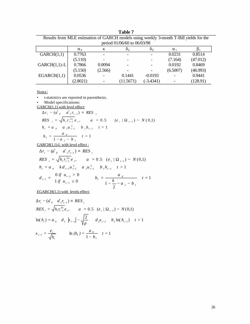
Table 7 Results from MLE estimation of GARCH models using weekly 3-month T-Bill yields for the

period 01/06/60 to 06/03/98 α0 κ δ1 δ2 α1 β1

GARCH(1,1) 0.7763 - - - 0.0231 0.8514 (5.110) - - - (7.164) (47.012)

GARCH(1,1)-L 0.7866 0.0094 - - 0.0192 0.8469 (5.150) (2.566) - - (6.5007) (46.993)

EGARCH(1,1) 0.0536 - 0.1441 -0.0193 - 0.9441 (2.8021) - (11.5671) (-3.4341) - (128.91)

Notes: • t-statistics are reported in parenthesis. • Model specifications: GARCH(1,1) with level effect:

GARCH(1,1)-L with level effect :

EGARCH(1,1) with levels effect:

1 1

1

)1,0(~)|( 5.0 ,

)ˆˆ(

11

01

112

110

12

1

110

=−−

=

>++=

Ω==

≡+−∆

−−

−−

−

th

t huh

NrhRES

RESrr

ttt

tttttt

ttt

βαα

βαα

εαε

ααα

1

21

0 10 0

1

)1,0(~)|( 5.0 ,

)ˆˆ(

11

01

1

11

112

112

110

12

1

110

=−−−

=

≤>

=

>+++=

Ω==

≡+−∆

−

−−

−−−−

−−

−

thuifuif

d

t huudh

NrhRES

RESrr

t

tt

ttttt

tttttt

ttt

βακ

α

βακα

εαε

ααα

1 1

ln

1 )ln(2

)ln(

)1,0(~)|( 5.0 ,

)ˆˆ(

1

011

1112110

12

1

110

=−

==

>++

−+=

Ω==

≡+−∆

−

−−−

−−

−

t)(hh

t hh

NrhRES

RESrr

t

tt

tttt

tttttt

ttt

βαε

ξ

βξδπ

ξδα

εαε

ααα

Table 8 In-sample comparison of alternative models for the entire sample period

01/06/60 to 06/03/98 (sample size: 2003)

number of parameters

Log-Likelihood

AIC SBC Adj R2 Odds ratios

Constant Variance 1 -8589.23 -8590.23 -8593.03 -0.477 - GARCH(1,1) 3 -7965.81 -7968.81 -7977.22 0.222 623.42

GARCH(1,1)-L 4 -7962.05 -7966.05 -7977.25 0.205 627.18 EGARCH(1,1) 4 -7953.13 -7957.13 -7968.34 0.220 636.1

SSV model 3 -7825.64 -7828.64 -7837.04 0.405 763.59 RSV model 6 -7397.39 -7401.39 -7412.60 0.602 1191.84

Notes: • AIC: log-likelihood value less number of parameters • SBC: log-likelihood value less 0.5 log (T*number of parameters )

where T: sample size

• MSE:

[ ]T

hREST

ttt∑

=

−1

22

• MAE: T

hREST

ttt∑

=

−1

2

• Adj R2: Adjusted R2 is calculated for the regression ),~N( uubhas tttt 10 Re 2 ++= t= 1,…..N,

where RESt are the residuals from regressing ∆rt against constant and ∆rt-1 and ht t= 1,…..N are conditional volatility estimates

• Odds ratio: the posterior odds ratio of alternative specifications relative to the constant variance. This is obtained as difference of the Schwartz Bayesian Criterion (SBC) of each competing model and the SBC of the constant variance model –see, Kim and Kon (1994).

• All the models used here are described in Tables 3-7.

Table 9 In-sample and out-of-sample comparison of alternative models for three different sample periods

Sample 1

In-sample (T: 990) 01/06/60-31/12/78

Out-of-sample (T:1012) 01/01/79-06/03/98

MSE MAE Adj. R2 MSE MAE Const. Variance 0.0109 0.0266 -0.0495 0.0702 0.0682 EGARCH(1,1) 0.0104 0.0255 0.104 0.0707 0.0694

SSV model 0.0104 0.0255 0.409 0.0706 0.0688 RSV model 0.0099 0.0243 0.615 0.0705 0.0685

Sample 2

In-sample (T: 1199) 01/06/60-31/12/82

Out-of-sample (T:803) 01/01/83-06/03/98

MSE MAE Adj. R2 MSE MAE Const. Variance 0.0661 0.0714 -0.0671 0.0025 0.0132 EGARCH(1,1) 0.0621 0.0679 0.210 0.0027 0.0130

SSV model 0.0628 0.0680 0.485 0.0026 0.0126 RSV model 0.0616 0.0668 0.612 0.0026 0.0123

Sample 3

In-sample (T: 1668) 01/06/60-31/12/91

Out-of-sample (T:334) 01/01/92-06/03/98

MSE MAE Adj. R2 MSE MAE Const. Variance 0.0489 0.0561 -0.0562 0.0002 0.0067 EGARCH(1,1) 0.0461 0.0538 0.212 0.0001 0.0049

SSV model 0.0464 0.0538 0.481 0.0001 0.0047 RSV model 0.0458 0.0532 0.603 0.0001 0.0047

Sample 4

In-sample (T: 626) 01/01/76-31/12/87

Out-of-sample (T:104) 01/01/88-31/12/89

MSE MAE Adj. R2 MSE MAE Const. Variance 0.1133 0.1081 -0.0993 0.0003 0.0119 EGARCH(1,1) 0.1090 0.1054 0.221 0.0005 0.0128

SSV model 0.1082 0.1051 0.494 0.0005 0.0124 RSV model 0.1031 0.1014 0.554 0.0003 0.0115

Notes: • T: refers to the sample size. • The best model is highlighted.

• MSE:

[ ]T

hREST

ttt∑

=

−1

22

• MAE: T

hREST

ttt∑

=

−1

2

• The estimated coefficients from the in-sample period are used to generate one-week (step) ahead conditional

29

volatility estimates for the out-of-sample period. One-step ahead conditional volatility forecasts are generated using the following equations (based on the GARCH models defined under Table 7 and the SV models 2 and 3):

GARCH(1,1):

GARCH(1,1)-L:

EGARCH(1,1):

SSV model:

RSV model:

11

00

02

|11

1102

|

1

)()(

βαα

σβασ

−−=

−++= +−

+

w

where

ww tts

tst

21

)()2

(

11

00

02

|11

1102

|

κβα

α

σκ

βασ

−−−=

−+++= +−

+

w

where

ww tts

tst

1

00

02

|11

102

|

1

))(ln()()ln(

βα

σβσ

−=

−+= +−

+

w

where

ww tts

tst

))(ln()()ln( 2|1

11

2| µσφµσ −+= +

−+ tt

stst

[ ][ ] )|1()|1()ln(

)|0()|0()ln()ln(

112

|

112

|2

|

−++−+++

−++−++++

=×=

+=×==

ststststtst

ststststtsttst

ssprsspr

ssprsspr

σ

σσ

30

Figure 1. Weekly 3-month T-Bill percentage yields (Sample: 01/06/60 to 06/03/98)

31

Figure 2. Posterior Density Plots for Parameters of the SSV Model

Figure 3. Posterior Density Plots for Parameters of the RSV model

32

Figure 4. Gibbs Run for Parameters of the RSV Model

Figure 5. Autocorrelation Functions for Parameters of the RSV Model

33

Figure 6. T-Bill Yields and Corresponding Latent Volatility and States (Sample: 01/06/60 to 06/03/98)

34

Figure 7. Comparison of in-sample Conditional Volatilities Across Different Models

(Sample: 01/06/60 to 06/03/98)