Reducing False Alarms with Multi-modal Sensing for ...johnh/PAPERS/Zhang13b.pdf · Reducing False Alarms with Multi-modal Sensing for Pipeline Blockage (Extended) ... machine wear-out

Reducing False Alarms with Multi-modal Sensingfor Pipeline Blockage (Extended) ∗

ISI Technical Report ISI-TR-2013-686b

June 2013 (revised 3 July 2013)†

Chengjie ZhangInformation Sciences Institute

University of Southern CaliforniaMarina del Rey, California, USA

[email protected]

John HeidemannInformation Sciences Institute

University of Southern CaliforniaMarina del Rey, California, USA

[email protected]

AbstractIndustrial sensing applications place a premium on cost-

effectiveness and accuracy. Traditional approaches oftenuse expensive, invasive sensors, because inexpensive sensorssuffer from false positive detections. Sensor cost means au-tomation is sparse or avoided when the value of specific sitescannot be justified. In this paper, we show combining dif-ferent types of sensors can allow low-cost sensors to avoidfalse positives, enable much greater levels of automation insome applications. We explore this problem by studying aspecific application: blockages in oil flowline common incold weather. We use pipe skin temperature to infer changesin fluid flow, and combine readings with acoustic data toavoid false positives and be robust to environmental changes.We demonstrate that our approach is effective with field ex-periments. Finally, suggest that this approach generalizesto other classes of problems where false positives from onesensing modality can be resolved by multi-modal sensing.

1 IntroductionSensor networks are used to collect data, detect prob-

lems, and take actions in the physical world. Small andinexpensive, sensornets can be easily deployed to addressmany real-world problems, from sewage pipe leakage detec-tion [37], milling machine wear-out prediction [51] and livestock health monitoring [9].

In spite of their effectiveness in some applications, sen-sornet uptake has been slow in many industrial applications.SCADA systems today often employ traditional dedicatedand often expensive sensors, or fall back on manual observa-tions where automated sensing is not seen as cost effective.A challenge in use of low-cost wireless sensors is that sim-ple sensing methods often create many false alarms whenthey are confused by noise or changes in regular operation.

In this paper we propose to use different kinds of sensorsto distinguish real anomalies from false alarms. We select amain sensor that detects the anomaly but may be confusedby changes during regular operation. We then add additionalsensors that can distinguish actual problems from false posi-tives, although they cannot detect anomalies alone.

∗ This research is partially supported by CiSoft (Center for In-teractive Smart Oilfield Technologies), a Center of Research Ex-cellence and Academic Training and a joint venture between theUniversity of Southern California and Chevron Corporation.

† Revisions in July include correction of typos and small clar-ifications in Section 2.1, 2.3, 2.4, 4.2, 4.4, 4.6 and 5.1.2.

Our overall goal is to identify classes of industrial appli-cations where multi-modal sensing can resolve sensing am-biguities. In this paper we prove this claim in the context ofa specific example: cold-oil blockages in flowlines in pro-ducing oilfields. A typical oilfield has many kilometers ofdistribution flowlines that collect crude oil extracted fromwellhead pumpjacks, gathers the oil for measurement andaccounting, and ultimately sends it to refineries. Distribu-tion systems near the wellhead are often small, particularlyin older fields. In cold weather, oil thickens because oil vis-cosity has an inverse proportional relation with its tempera-ture. Oil may then interact with sand or other contaminantsin the fluid, and with pipe sags or narrow fittings, resultingin blockages in the lines. Blocks cause production loss, andif left unresolved they can result in pipe leaks, damage tothe flowline, or even to the pumpjack. After pipe being fullyclosed, it takes only tens of seconds for pressure to build upbefore some parts in line rupture.

Although the oil industry has explored several stand-alonesensors, current approaches are either unreliable or too ex-pensive to install and maintain (Section 2.1). Although somefields contain thousands of wells where production lines arevulnerable to blockage, manual inspection is the most com-monly used technique today.

Our insight is that multi-modal sensing can not only re-duce the cost of detection of cold-oil blockages while avoid-ing false alarms. Automating sensing can provide muchmore rapid detection than current approaches. Rapid feed-back is important because a shorter gap between blockagereaches critical level and alarm is signaled can minimize dif-ferent losses, including environmental and equipment. Wedetect blockage by sensing temperature and acoustic signals.We infer flow interruption from pipe skin temperature, but inaddition to blockages, many regular events change tempera-ture, including automatic pumpjack shut-ins and diurnal en-vironmental effects. We avoid false positives by comparingmultiple temperature readings and by using acoustic sensingto monitor pumpjack status. We define our sensing problemand summarize our approach in Section 2.1.

Our experimental results focus on cold-oil blockage, butthe principle of multi-modal sensing to avoid false positivesapplies to many other sensing problems. For example, Girodand Estrin suggest using video evidence to correct prob-lems from obstacles in acoustic ranging [10]. In human mo-tion detection, Stiefmeier et al. cross-segment data streambetween different sensors, including inertial, vibration and

force sensitive sensors [36]. We discuss more on generaliz-ing our approach to other applications in Section 4.10.

The first contribution of this paper is to identify the op-portunity for multi-modal sensing to reduce error rates withlow-cost sensors. While some prior sensors have exploredmulti-modal sensing with expensive sensors (for example,cameras [10]) and PC-level computation (including mobilephones or laptops [3,51]), we believe we are the first to showthese approaches apply to low-cost embedded sensors.

Our second contribution is to prove this claim by explor-ing a specific application: we design an embedded sensingapproach that detects cold-oil line blockages using a combi-nation of inexpensive temperature and acoustic sensors (Sec-tion 2), then test our specific implementation (Section 3) inthe field (Section 4).

2 Design of Cold-Oil Blockage Detection Al-gorithm

Here we define the problem we are solving, then explorehow low-cost temperature sensors detect blockage, acous-tic sensors detect equipment operation, and the two togetherprovide reliable blockage detection with a low false positiverate.

2.1 Problem StatementThe goal of this paper is to understand how sensing can

assist industrial applications, and how multi-modal sensingcan help avoid false positives. While in the abstract, multi-modal sensing is straightforward, the key question is under-standing how real-world sources of noise and false detec-tions affect sensing system design. To that end, we focus oncold-oil blockage as a real-world application.

The Problem: Cold-oil blockage occurs when the returnline from a producing oil well becomes blocked, typicallydue to changes in oil viscosity as a result of cold weather,sometimes compounded by buildup of sand in the pipe.

Blockage typically build up gradually over time. Produc-ing wells often operate intermittently with on/off cycles of5-15 minutes (to allow downhole pressure to build up forsuitable operation); when the pump is not operational, oilcan transition from flowing slowly to blocked. A blockedpipe can cause equipment damage and oil leaks, since if wellproduction continues with a blocked flow line pressure inthe line will cause flow line rupture or pumpjack damage.Recovery from equipment damage can easily amount to tenthousand dollars per event, in addition to reducing produc-tion.

Cold-oil blockage is a significant problem in some oil-fields. Figure 1 shows eight consecutive years of produc-tion data of an oil field where cold-oil blockage is a con-cern. We normalize production values to remove long-termdecreasing trend in field production and show seasonal vari-ation in production. The first step of normalization is com-puting monthly index by applying exponential decay fittingover the whole dataset. The resulting fitting error is 1.3%,low enough to show we have a good fit. The fitting forecastis the monthly index—the baseline of monthly productionwhich is unaffected by the overall trend. Next, we normal-ize the raw data by its ratio against its index for every monthand the result is in the upper plot. The lower plot summa-

JAN FEB MAR APR MAY JUN JUL AUG SEP OCT NOV DEC95%

100%

105%

no

rmal

ized

pro

du

ct.

0%

50%

100%

% b

elo

w b

asel

ine

Figure 1. Seasonality analysis shows winter productionloss.

rizes, for each month, how often that month’s production isbelow its index. It further shows that winter months (Novem-ber through February) witness consistently lower productionrates. There are multiple factors that contribute to this trend(scheduled maintenance is often planed to avoid hot summermonths), but field engineers confirm that a significant factorto reduced winter production are well problems due to cold-oil blockage.

Although we focus on cold-oil blockage so can evaluatereal-world sources of error, in Section 4.10 we consider howmulti-modal sensing applies in other applications.

Current Approaches: Aware of the problem, oil com-panies have explored current sensing approaches, includingflowmeters, pressure sensors, leak detection, and of coursemanual inspection. Unfortunately, currently techniques forautomation have high installation and maintenance costs.For example, pressure sensors cost US$1 000 or more to pur-chase and have annual costs of $300 or more to recalibrate;flow sensors are more costly. As a result, these sensors areused only on a few, very productive wells, while manual in-spection remains common, in spite of its large delay.

These approaches suggest the importance of the problem,but sensor cost means they are deployed on only a few ofthe thousands of wells where there is concern. Field engi-neers confirm that in some cases, the alternative is simplyto preemptively stop production on certain well that have nomonitoring.

Degree of Blockage: Blockages build up over time, andone would like to detect them before they happen, or veryquickly after they happen. Currently pressure sensors aredeployed on only a few wells. Instead, manual inspection isdone to identify equipment damage that follows a blocking,something that often occurs twelve hours after the fact.

Here we focus on rapid detection of full and near-fullblockages. Detection of blockage allows well shut-in andrecovery before damage; rapid detection after blockage mayavoid equipment damage and will minimize leaks. Our eval-uation (Section 4.7) shows we can detect blockage in 10 to30 minutes, much shorter than 12 hours by current manualinspection. While not instantaneous, this detection is poten-tially able to save large production loss.

We emulate full blockages in field experiments (Sec-tion 4). We cannot test near-full blockages in the field dueto safety concerns, but we do evaluate near-full blockages in

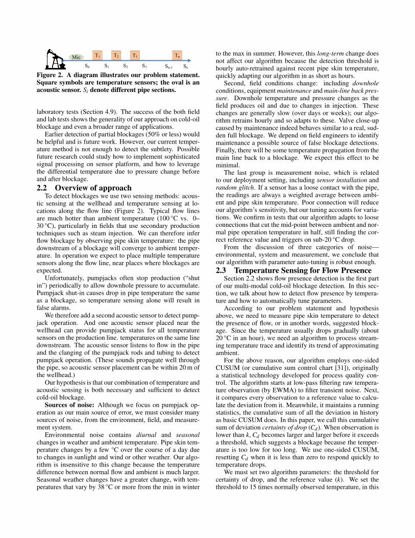
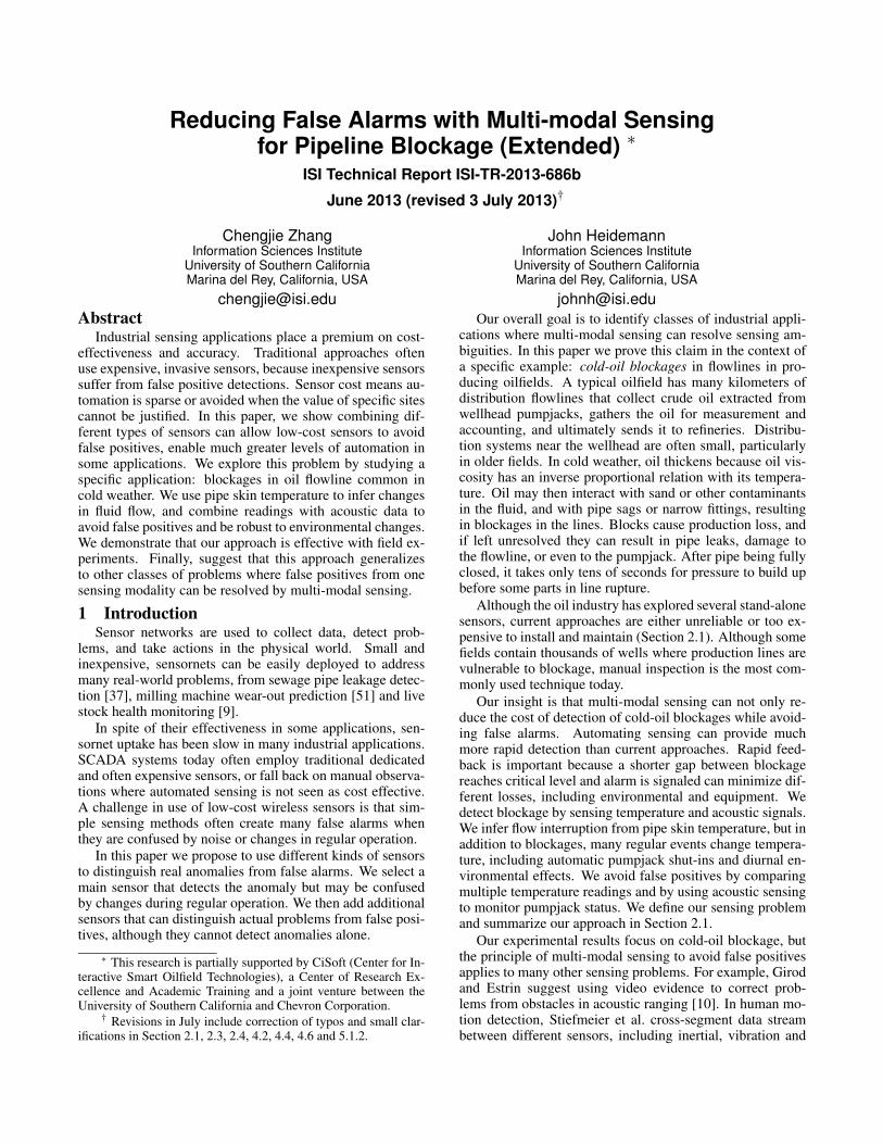
Figure 2. A diagram illustrates our problem statement.Square symbols are temperature sensors; the oval is anacoustic sensor. Si denote different pipe sections.

laboratory tests (Section 4.9). The success of the both fieldand lab tests shows the generality of our approach on cold-oilblockage and even a broader range of applications.

Earlier detection of partial blockages (50% or less) wouldbe helpful and is future work. However, our current temper-ature method is not enough to detect the subtlety. Possiblefuture research could study how to implement sophisticatedsignal processing on sensor platform, and how to leveragethe differential temperature due to pressure change beforeand after blockage.

2.2 Overview of approachTo detect blockages we use two sensing methods: acous-

tic sensing at the wellhead and temperature sensing at lo-cations along the flow line (Figure 2). Typical flow linesare much hotter than ambient temperature (100 °C vs. 0–30 °C), particularly in fields that use secondary productiontechniques such as steam injection. We can therefore inferflow blockage by observing pipe skin temperature: the pipedownstream of a blockage will converge to ambient temper-ature. In operation we expect to place multiple temperaturesensors along the flow line, near places where blockages areexpected.

Unfortunately, pumpjacks often stop production (“shutin”) periodically to allow downhole pressure to accumulate.Pumpjack shut-in causes drop in pipe temperature the sameas a blockage, so temperature sensing alone will result infalse alarms.

We therefore add a second acoustic sensor to detect pump-jack operation. And one acoustic sensor placed near thewellhead can provide pumpjack status for all temperaturesensors on the production line. temperatures on the same linedownstream. The acoustic sensor listens to flow in the pipeand the clanging of the pumpjack rods and tubing to detectpumpjack operation. (These sounds propagate well throughthe pipe, so acoustic sensor placement can be within 20 m ofthe wellhead.)

Our hypothesis is that our combination of temperature andacoustic sensing is both necessary and sufficient to detectcold-oil blockage.

Sources of noise: Although we focus on pumpjack op-eration as our main source of error, we must consider manysources of noise, from the environment, field, and measure-ment system.

Environmental noise contains diurnal and seasonalchanges in weather and ambient temperature. Pipe skin tem-perature changes by a few °C over the course of a day dueto changes in sunlight and wind or other weather. Our algo-rithm is insensitive to this change because the temperaturedifference between normal flow and ambient is much larger.Seasonal weather changes have a greater change, with tem-peratures that vary by 38 °C or more from the min in winter

to the max in summer. However, this long-term change doesnot affect our algorithm because the detection threshold ishourly auto-retrained against recent pipe skin temperature,quickly adapting our algorithm in as short as hours.

Second, field conditions change: including downholeconditions, equipment maintenance and main-line back pres-sure. Downhole temperature and pressure changes as thefield produces oil and due to changes in injection. Thesechanges are generally slow (over days or weeks); our algo-rithm retrains hourly and so adapts to these. Valve close-upcaused by maintenance indeed behaves similar to a real, sud-den full blockage. We depend on field engineers to identifymaintenance a possible source of false blockage detections.Finally, there will be some temperature propagation from themain line back to a blockage. We expect this effect to beminimal.

The last group is measurement noise, which is relatedto our deployment setting, including sensor installation andrandom glitch. If a sensor has a loose contact with the pipe,the readings are always a weighted average between ambi-ent and pipe skin temperature. Poor connection will reduceour algorithm’s sensitivity, but our tuning accounts for varia-tions. We confirm in tests that our algorithm adapts to looseconnections that cut the mid-point between ambient and nor-mal pipe operation temperature in half, still finding the cor-rect reference value and triggers on sub-20 °C drop.

From the discussion of three categories of noise—environmental, system and measurement, we conclude thatour algorithm with parameter auto-tuning is robust enough.

2.3 Temperature Sensing for Flow PresenceSection 2.2 shows flow presence detection is the first part

of our multi-modal cold-oil blockage detection. In this sec-tion, we talk about how to detect flow presence by tempera-ture and how to automatically tune parameters.

According to our problem statement and hypothesisabove, we need to measure pipe skin temperature to detectthe presence of flow, or in another words, suggested block-age. Since the temperature usually drops gradually (about20 °C in an hour), we need an algorithm to process stream-ing temperature trace and identify its trend of approximatingambient.

For the above reason, our algorithm employs one-sidedCUSUM (or cumulative sum control chart [31]), originallya statistical technology developed for process quality con-trol. The algorithm starts at low-pass filtering raw tempera-ture observation (by EWMA) to filter transient noise. Next,it compares every observation to a reference value to calcu-late the deviation from it. Meanwhile, it maintains a runningstatistics, the cumulative sum of all the deviation in historyas basic CUSUM does. In this paper, we call this cumulativesum of deviation certainty of drop (Cd). When observation islower than k, Cd becomes larger and larger before it exceedsa threshold, which suggests a blockage because the temper-ature is too low for too long. We use one-sided CUSUM,resetting Cd when it is less than zero to respond quickly totemperature drops.

We must set two algorithm parameters: the threshold forcertainty of drop, and the reference value (k). We set thethreshold to 15 times normally observed temperature, in this

case 3 000, to be robust to transient temperature dips. Thereference value, k is set as the mid-point between qualitylevel—normal pipe temperature, µ0 and anomaly level—flowstopped, µ1 (µ1 < µ0).

Since k is important to the accuracy and responsiveness ofthe algorithm, we auto-tune it instead of hard-coding. How-ever, due to different sources of noise we list in problemstatement, we do not think predefined, fixed µ0 and µ1 es-timation can best reflect an appropriate k. Hence, it is nec-essary to first auto-tune µ0 and µ1 for its dependency and weembed auto-tuning in our algorithm to adjust the estimationof the two levels. When pumpjack is operating (determinedby acoustic node, introduced later in Section 2.4), we con-stantly update the quality level µ0 by temperature observa-tion. When pumpjack shuts in, we stop updating µ0 but startanomaly level µ1 updating as temperature drops. To general-ize this, we are using a second sensory channel, to convert afalse-alarm hazard into a helper of parameter tuning. By thetime of the shut-in is over and pumpjack resumes operating,a new reference value k will be ready, based on auto-tuned µo

and µ1. Another k-tuning feature is that we do not update k atshut-in because during pump-off, temperature detection be-comes less important. More importantly, we intend to avoidaccidentally updating threshold to an inappropriate value.

2.4 Acoustic Sensing to Avoid False AlarmsOur discussion in Section 2.1 shows that temperature

alone is not enough. Acoustic sensing on pumpjack statuscan avoid the false alarms caused by regular pump-off. Inthis section, we describe our acoustic algorithm design andnext discuss how we automatically tune parameters in thatalgorithm.

We need to determine if pumpjack is operating for endpipe blockage detection. Since pumpjack stroke with enginerumbling generates wide band noise and propagates alongpipe, we use microphone mounted on pipe surface to mea-sure the sound pressure level (SPL), a high level of whichsuggests pumpjack operating. When pumpjack is off, micro-phones are expected to pick up much lower energy of envi-ronmental noise.

Our acoustic algorithm works as follows. First, for eachstroke cycle C, we detect if pumpjack is on by comparingsound amplitude to a pre-configured threshold θp. If sam-ples in C exceeds the threshold, mostly because of a signifi-cantly loud rod-tube clang noise associated with each stroke,we decide the pumpjack is on during the whole cycle (typ-ically 7 s). However, simple pumpjack flip detection is notrobust against transient error and hence we need to know ifthe pumpjack is steady on. In order to make that decision, wecheck a longer history to see if it was being on for a wholewarm-up period W long, usually far longer than a single cy-cle.

Hence, to correctly detect pumpjack status, we need toproperly configure three parameters: certainty of drop (C),warm-up period (W ), and threshold (θp). We do tuning onbase station because the training involves certain intensivecomputation as auto-correlation and memory storage com-plexity both beyond mote capacity; so we employ a PC inour experiments. (In principle a mobile-phone class proces-sor could easily accommodate this work, although it is be-

yond 8-bit motes.) The on-site training step makes acous-tic sensors robust against environment noise and mechanicaldifference across pumpjacks. We next describe our trainingalgorithm for these three parameters, started by training datacollection.

Before deployment, we collect a short period of acoustictraining data containing both pump-on and -off. We nextcompute C by running auto-correlation over the pump-ontrace. The lag yielding the largest coefficient representspumpstroke cycle. To prevent from choosing harmonics,in implementation we search the highest coefficient in apossible-cycle range, say [5 s, 9 s]. Further, based on ourprior study, W could be set as five times of C.

We consider both pump-on and -off to compute θp, be-cause it needs to be able to properly denote the differencebetween those two status. We first compute the noise floorby averaging all the samples in pump-off trace. We nextthrow away all samples below noise floor in pump-on seg-mentation. θp equals the 86-percentile of amplitude amongall the rest of the pump-on segmentation. The reason wechoose this value for θp is that during a common 7 s pumpcycle, our threshold should detect the single sample captur-ing the loudest rod-tube clang noise against other six under1 Hz sampling rate. Therefore, the signature noise sample islikely to have a higher amplitude than the other 86% (six outof seven in one cycle) samples.

2.5 Sensor Fusion for Blockage DetectionWe talk about the two algorithms in the above sections

and next we describe how to fuse them to detect end block-age. If we interpret our basic hypothesis (Section 2.1) withtechnical details, we find that blockage could be detectedas flow stops but pump is steady on. In another words, ifpumpjack is off, our algorithm ignores all suggested block-age detection by temperature sensing, although the certaintyof drop builds up due to stagnant flow.

On the contrary, if pumpjack is on, our algorithm can de-tect blockage, all in the following two different situations. Ifblockage occurs during pumpjack operation (i.e. pumpjack issteady on), we expect to witness a line temperature drop. Assoon as line temperature stays below reference value longenough, blockage detection triggers. Besides, if blockageoccurs during shut-in, after pipe cools off and pumpjack re-sumes, line temperature stays close to ambient and does notincrease significantly. Hence, the certainty of drop can toobuild-up, followed by blockage detection. We evaluate thefusion result later in Section 4.7.

3 System ImplementationBefore we review the details of our field experiment, we

briefly talk about the implementation of our mote sensingplatform with low-cost sensors. We first briefly summarizethe hardware of our multi-modal sensing system. Next, wediscuss the two challenges in acoustic node implementationand our software approaches to solve them.

3.1 System HardwareOur sensor network consists of three types of nodes: base

node for data collection, acoustic mote for pumpjack statusdetection and temperature mote for flow presence detection.In this section, we introduce the hardware of their parts.

Our base node is simply a Mica-2 mote [40] connected toPC through MIB520 programming board. It passively listensand logs all the packets transmitted from acoustic or temper-ature motes in the network.

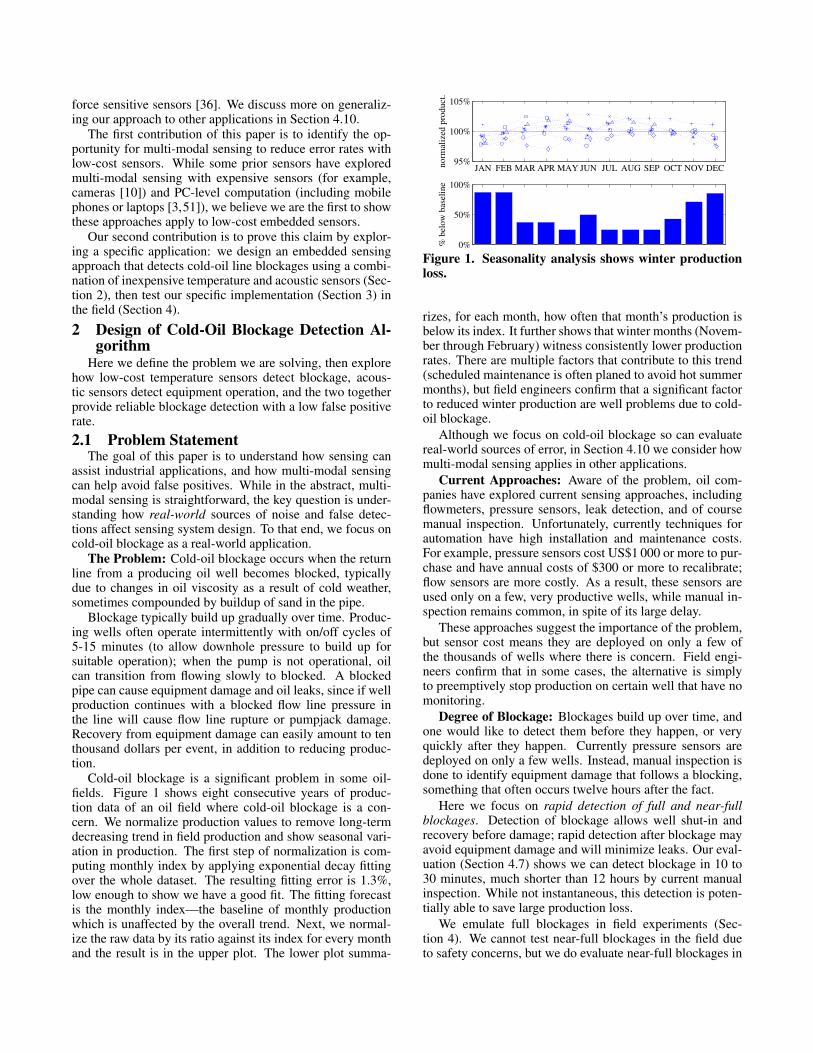
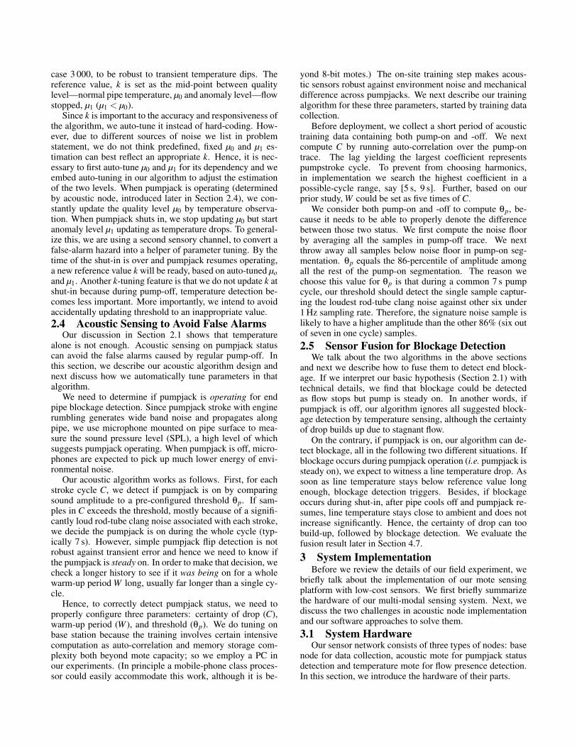
Our acoustic mote is composed of a Mica-2 mote and anMTS310CA, “Mica Sensor Board” with an on-board electretcondenser microphone, Panasonic WM-62A (Figure 3(a)).Figure 3(b) shows how we tape and clamp the extended mi-crophone on the pipe with thermal insulation and we discusshow decoupling microphone benefits signal gain later.

We cannot directly mount Mica-2 microphone on pipebecause the high pipe temperature may damage the equip-ment, or at least result in inaccurate measurement. Com-mon electret condenser microphone has a sub-70 °C opera-tion temperature, lower than the pipe skin temperature in op-eration. Although it is not mentioned in its specification [46],we believe this model on Mica sensor board, WM-62A isnot designed for a higher temperature task. Even if it sus-tains the heat, electret condenser microphone has an unpre-dictable frequency response under high temperature (around80 °C [49]). Therefore in deployment, we apply thermal in-sulation on top of the over-warm pipe to protect our micro-phone. The insulation is called Fire Blanket and is made ofwoven fiberglass. We are aware of some side effects of sand-wiching insulation between the microphone and pipe, for ex-ample, signal attenuation. However, under the design prin-ciple of low-cost sensing, we decide to make this trade-offinstead of employing expensive specially-customized micro-phones, say US$5 000-priced Bruel & Kjær 4949 automotivesurface microphone.

Finally, the design principle of temperature motes inher-its our prior work [52]. They each consists of a Mica-2 forcontrol, a custom amplifier board to optimize thermocouplesignal readings and a thermocouple sensor (NANMAC D6-60-J J-type) for pipe line and ambient temperature measure-ments. Figure 3(c) and 3(d) shows how we deploy them inour experiment.

During experiments, we were surprised to find that ourcustom amplifier boards are sensitive to their operation tem-perature, although all components are rated at a much higherrange. Our initial field trials show if exposed under the sundirectly, temperature sensors with the amplifiers sometimesreturn random readings, but sensors without the amplifierswork correctly. Hence in the latest test (Section 4.2), wecovered the sensor motes in shade, but we are currently ex-amining our design and seeking a more robust solution.

3.2 Hierarchical Sampling and Aggregationin Acoustic Mote

To obtain the sound pressure level of pipe, our acousticsensor samples 2 000 times a second. This sampling rateis high for a mote, posing two challenges. First, althoughthe sensor generate and transmit one packet per second, wecannot collectively stack 2 000 (one-second-long) samples inbuffer due to the limited Mica-2 RAM size (4 kB for bothprogram and data). The other challenge is that because thesensor samples at such short interval as 500 µs, hardware in-terrupts from other components (radio, flash logger, etc) arelikely to cause large variation in sampling rate [14, 18]. For

accurate sampling, we shut down all external componentswhich might occupy the CPU for too long to hold up thetimer. Hence, we design our software able to schedule andinterleave processing, transmitting and flash logging amongcontinual sampling. We do local flash logging because inoperation, it could serve as backup in case of temporary net-work outages, although in a fully integrated system, data isalways streamed back to a central server through field net-work.

We design a hierarchical sampling and aggregationscheme to overcome the two challenges above. Overall, wepause the high frequency sampling and schedule other oper-ations, before next sampling cycle. The pause causes gaps insampling, and in the worst case we may mis-detect interest-ing phenomenon. To minimize this sampling gap and coor-dinate data management, we make following design choices.At a high level, our sensor samples and computes the SPLwithin a one-second-long window (long window) before log-ging it to flash and transmitting it out. At an intermediatelevel, we divide each long window into ten 0.1-second-longshort windows. In each short window, sensor samples for0.06 s at 2 kHz rate, and uses the remaining 0.04 s to do SPLaggregation. The final 10th short window does further aggre-gation by choosing the maximum SPL value among the pastten to represent the entire long window, before flash loggingand radio transmission. Our lab testing shows 60%/40% dutycycle is optimal because a slightly more aggressive setting(i.e. short than 0.04 s gap) causes significantly more packetloss. Besides, the 0.04 s gap does not cause mis-detection onthe 0.2-second-long signature rod-tube clanging noise.

3.3 Maximizing Acoustic GainTo maximize the acoustic signal gain, we take three steps

on software and hardware customization.First, we optimally adjust digital current bias through cal-

ibration. The 10-bit ADC channel of Mica-2 returns valuesranging from 0 to 1023 mapped to 0 to 3 V. As a result, itdoes not return negative voltage. To avoid losing the nega-tive half of the waveform, MTS310CA is designed to elevatethe center of the output acoustic waveform from 0 V to ap-proximately 1.5 V, which corresponds to 512 in ADC value.We test this feature with our equipment and find that the newADC waveform centers around 501, slightly off by the theo-retical value of 512. We thus use our experimental result tooffset mote ADC readings, removing DC bias.

Second, we decouple microphone unit from the board forbetter mounting. The flat Mica sensor board does not wellmatch the curved pipe surface. Therefore, we desolder themicrophone off and extend it out via wire, which enables usto simply tape it down to pipe in deployment for best contactand windscreen.

Finally, we use TinyOS to maximize the microphone ana-log gain. We use the OS service to tune an resistor in theamplification stage to its largest value, which is an on-board,digitally controlled, variable resistor [41].

4 EvaluationWe next describe the experiments we carried out to

demonstrate we can detect flow blockage, and that multi-modal sensing can avoid false positives. We first evaluate

(a) Acoustic mote with microphoneextended

(b) Mote mic on a pipe (c) Temperature motepacked in a box

(d) Thermocouple on apipe.

Figure 3. Our temperature and acoustic sensor hardware and deployment.

our inexpensive sensors in the laboratory. We next describeour field experimental setup and evaluation metrics test howtemperature and acoustic sensors can infer blockages andequipment operation, and finally show how their combina-tion provides a robust system.

4.1 Calibrating Individual SensorsOur premise is that low-cost sensors are sufficient to de-

tect flow blockages. We next compare inexpensive mote-based temperature and acoustic sensors against high-qualityPC-based sensors to confirm that inexpensive sensors are“good enough”.

4.1.1 Temperature Sensor Measurement

We show our acoustic mote is close enough to groundtruth in previous section. Next we compare temperaturedata by mote against USB data logger to verify if our lowcost temperature collection solution performs well enough ornot. The major differences between the two systems lies inhardware and calibration. The software processes are likelythe same, although only limited information about USB datalogger disclosed by its manufacturer.

In our prior work [53], we find that in relatively lowtemperature range (0–200 °C), it is unnecessary to calibrateJ-type thermocouples before we deploy them in detectiontasks. Hence, our mote reports raw ADC readings whileUSB data loggers are pre-calibrated by manufacturer.

Our mote is almost equivalent to USB data logger becauseof the strong correlation between them pairewisely. It is 0.91

on Tu, 0.80 on T1d

and 0.83 on T2d

. We further visualize

one data set, T 2d as an example to better demonstrate that

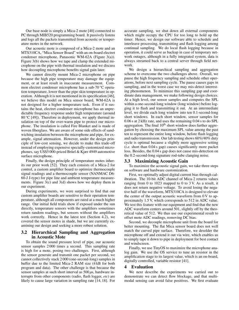
this claim. Figure 4 clearly shows that the data by mote ismerely off from ground truth by a constant but the fluctuationis almost the same. For clearer comparison, we post-facto’lyconvert raw ADC reading by mote to Celsius scale underfollowing equation [53]:

T = 18.259×ADC×3×1000

210×β

+2.852

where β is 367 as the gain of our pre-amplifier board. In ourdetection task, the algorithm is more sensitive to temperaturedrops instead of the absolute value, and hence a constant dis-parity is acceptable.

11:00AM 12:00PM 1:00PM 2:00PM 3:00PM 4:00PM 5:00PM0

20

40

60

80

100

tem

per

ature

(oC

)time

mote

USB

Figure 4. Temperature measured by mote and USB datalogger at T 2

d .

4.1.2 Acoustic Sensor MeasurementWe first look into our acoustic mote. Before we com-

pare mote and PC acoustic sensors, we briefly describestheir components and the difference in the data collectionapproaches. Our acoustic mote is consist of Mica-2 mote,an electret condenser microphone and a Mica sensor board.Whereas, our PC acoustic system is equipped with morepowerful hardware—a laptop with sound card complyingto Intel high definition audio architecture and a battery-powered lavalier microphone. The hardware superiority ofPC system alone is enough to justify its cleaner data.

Other than the hardware difference, the second major dif-ferences is sensor installation. Although both sit on top ofinsulation, we tape down mote microphone by duct tape topipe while we clamp on PC microphone by a customizedclasp and hose-clamps, likely to produce larger force to pressthe microphone against the pipe for a better contact.

Finally, there is difference in sampling and aggregationmechanism in software after we abstracted out the OS differ-ences, although the final packet rates of both for evaluationare the same, 1 Hz. As we described in Section 3, the rawsampling rate on motes is 2 kHz and we next use a hierarchi-cal aggregation to assemble one packet every second fromten 0.1-second-long short packets. On the other hand, theraw sampling rate on PC is 16 kHz, much high than whatwe have with motes, mainly because we plan to keep highquality ground truth data in case we need to investigate thefrequency domain of acoustic signal. Since the software wechoose, Audacity, does not support a sampling rate as low as1 Hz, and more importantly, we prefer to maintain the con-sistency between both systems, we re-sample our PC data in

11:00AM 12:00PM 1:00PM 2:00PM 3:00PM 4:00PM 5:00PM0

100

200

300

AD

C .

time

0

0.05

0.1

. am

pli

tude

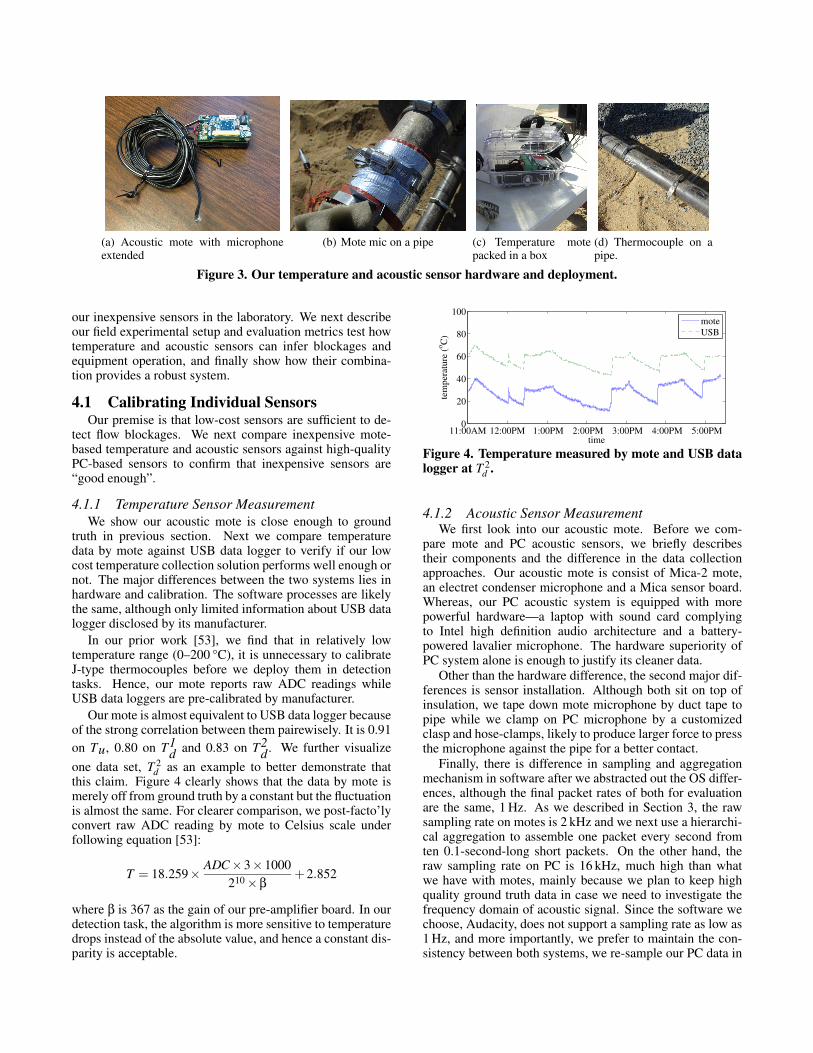
Figure 5. Acoustic measured by mote and PC micro-phone.

2 kHz by the same software before we further aggregate it byone-second-long window.

Despite the differences we listed above, Figure 5 showsthat our mote data is close enough to the ground truth. It isdifficult to directly convert their units; hence we keep bothtrace in their raw units and hand-scale them in the plot. Thecorrelation coefficient between the two traces is 0.44, prov-ing a strong positive correlation. The other observation thatPC data has higher SNR, which is depicted by much higherstate transition spikes and near-zero pump-off noise detec-tion.

In all through the comparison, we show our mote data isclose enough to PC data by a more expensive hardware suite.This result further supports our hypothesis above that lowcost sensor is capable of reaching effective yet economicalsensing.

4.2 Field Experiment ApproachWe next evaluate our system in field tests. From 9:30am

to 5:30pm, November 7th, 2012, we evaluated our systemand a producing oilfield in the California Central Valley,working with field engineers from our research partners whooperate that field. During the nearly seven-hour-long exper-iment, our system collected acoustic and temperature traces,did in-node processing and ran the full detection algorithm.We also collected ground truth data, concurrent with opera-tion of our experimental system. Ground truth temperatureand acoustic data employed USB thermocouple data loggers(EL-USB-TC [45]) and a laptop computer with a commoditymicrophone. Figure 6(b) shows the test site and the produc-ing wellhead.

Our experiment emulates oil blockages by controllingvalves. (We are not able to inject actual blockages, nor wasit the time of year when they would form naturally.) Fig-ure 6(a) illustrates the topology of sensors, pumpjack andvalves. Oval shape represents acoustic mote and squaresdo temperature ones. Tu is located before the production-circulation branch-out and so upstream to both valves. T 1

d

and T 2d are both on production line and straddle production

valve, downstream to Tu. To emulate blockages, we activatethe production valve to close because it is not practical to cre-ate a real blockage in the field. When we close the productionvalve, oil stops flowing in the pipe and hence we observe atotal blockage in line with the valve. In our experiment, wealways leave open either the production or circulation valve,since closing both could cause high pressure at the wellheadthat would damage the producing well or equipment.

Table 1. Experiment schedule and scheme.

product.

start pump valve purpose

11:01am onopen

T1,2

d learn µ0

11:11am off all learn µ1

12:01pm

on

close T1,2

d non-op

12:25pm open T1,2

d learn µ0

1:09pmclose

T1,2

d in-op

1:54pm off all learn µ1

2:35pm

on

open T1,2

d learn µ0

3:05pm close T1,2

d in-op

3:48pm

open

T1,2

d learn µ0

4:30pm* off all learn µ1

4:58pm on T1,2

d learn µ0

We conduct experiments on approximately half-hour in-tervals to allow the system time to stabilize between changes.Table 1 shows our schedule, with three pump-off periods forall four temperature motes to learn µ1 and update k, with thelast one (28-minute long) ran shorter than the first two (eachabout 50-minute-long) due to time constraint. According tothe blockage introduction in Section 2.1, in reality we maygenerally categorize blockage in to two types regarding howit is formed. One is caused by a lump of viscous oil or sandclogging narrow fitting during pumpjack operation (op), anin-op blockage. The other is caused by residue oil in pipecooling off and turning solid during shut-in before pumpjackresumes operation, a non-op blockage. To better evaluatethe generality of our algorithm, we simulate both types inthree instances over the course of the day, and each stage runsbetween 24 to 45 minutes. The simulations are interleavedwith other two types of stages. One is valve-open and pipetemperature rebounce, so sensors can learn normal pipe tem-perature µ0 during operation. The other is pumpjack shut-in, which configures the sensors’ CUSUM anomaly level µ1

(i.e.temperature on stagnant flow).In addition to this field test, we carry out two prior field

experiments where we evaluate components of our systemand collect ground truth data for analysis in the lab. Priortests were done at a different wellhead. We omit this datahere due to space, but replay of this ground truth data in thelab shows our system works correctly on another well withdifferent sensor locations.

4.3 Evaluation MetricsSection 2 shows that we detects cold-oil blockage by fil-

tering out irrelevant flow absence with acoustic pumpjackstatus detection. Before evaluation, we describe below thetemperature and acoustic detection metrics due to their sim-ilarity.

We evaluate both temperature and acoustic sensing in anevent-based manner, but with separate event definition. Fortemperature, one event is one interval between changes ofequipment setting, because we care about if flow presence

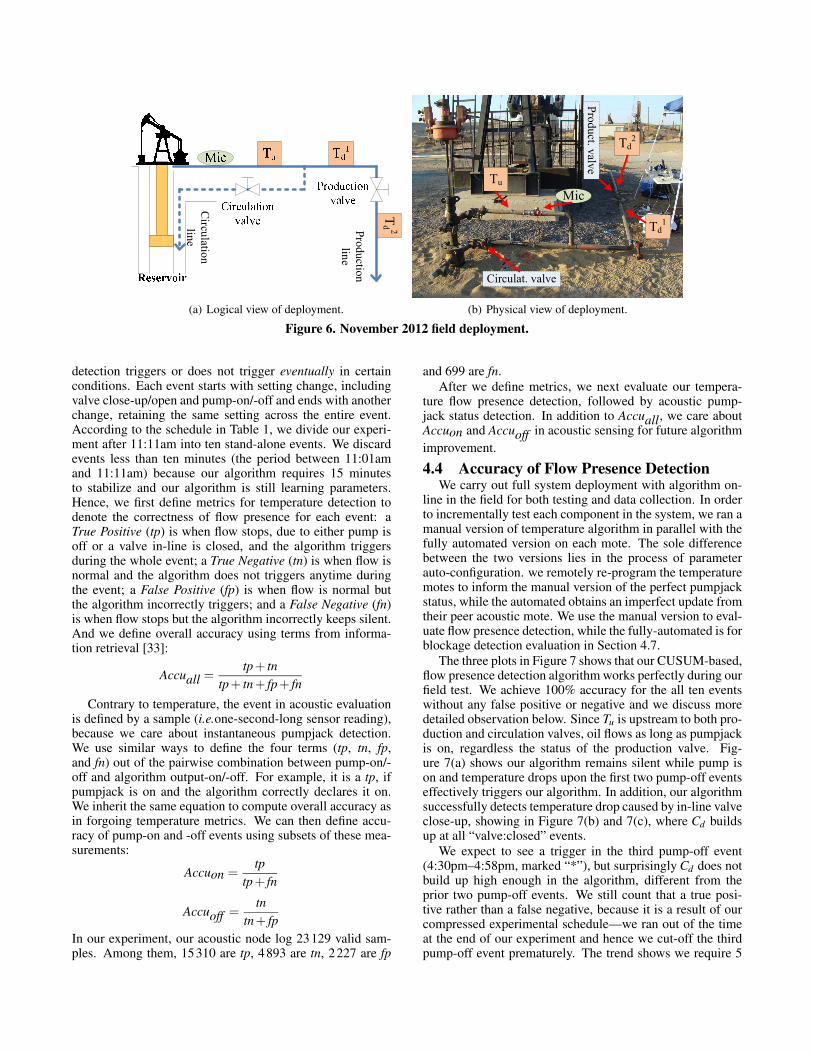
(a) Logical view of deployment.

(b) Physical view of deployment.

Figure 6. November 2012 field deployment.

detection triggers or does not trigger eventually in certainconditions. Each event starts with setting change, includingvalve close-up/open and pump-on/-off and ends with anotherchange, retaining the same setting across the entire event.According to the schedule in Table 1, we divide our experi-ment after 11:11am into ten stand-alone events. We discardevents less than ten minutes (the period between 11:01amand 11:11am) because our algorithm requires 15 minutesto stabilize and our algorithm is still learning parameters.Hence, we first define metrics for temperature detection todenote the correctness of flow presence for each event: aTrue Positive (tp) is when flow stops, due to either pump isoff or a valve in-line is closed, and the algorithm triggersduring the whole event; a True Negative (tn) is when flow isnormal and the algorithm does not triggers anytime duringthe event; a False Positive (fp) is when flow is normal butthe algorithm incorrectly triggers; and a False Negative (fn)is when flow stops but the algorithm incorrectly keeps silent.And we define overall accuracy using terms from informa-tion retrieval [33]:

Accuall =tp+ tn

tp+ tn+ fp+ fn

Contrary to temperature, the event in acoustic evaluationis defined by a sample (i.e.one-second-long sensor reading),because we care about instantaneous pumpjack detection.We use similar ways to define the four terms (tp, tn, fp,and fn) out of the pairwise combination between pump-on/-off and algorithm output-on/-off. For example, it is a tp, ifpumpjack is on and the algorithm correctly declares it on.We inherit the same equation to compute overall accuracy asin forgoing temperature metrics. We can then define accu-racy of pump-on and -off events using subsets of these mea-surements:

Accuon =tp

tp+ fn

Accuoff =tn

tn+ fp

In our experiment, our acoustic node log 23129 valid sam-ples. Among them, 15310 are tp, 4893 are tn, 2227 are fp

and 699 are fn.After we define metrics, we next evaluate our tempera-

ture flow presence detection, followed by acoustic pump-jack status detection. In addition to Accuall, we care aboutAccuon and Accuoff in acoustic sensing for future algorithm

improvement.

4.4 Accuracy of Flow Presence DetectionWe carry out full system deployment with algorithm on-

line in the field for both testing and data collection. In orderto incrementally test each component in the system, we ran amanual version of temperature algorithm in parallel with thefully automated version on each mote. The sole differencebetween the two versions lies in the process of parameterauto-configuration. we remotely re-program the temperaturemotes to inform the manual version of the perfect pumpjackstatus, while the automated obtains an imperfect update fromtheir peer acoustic mote. We use the manual version to eval-uate flow presence detection, while the fully-automated is forblockage detection evaluation in Section 4.7.

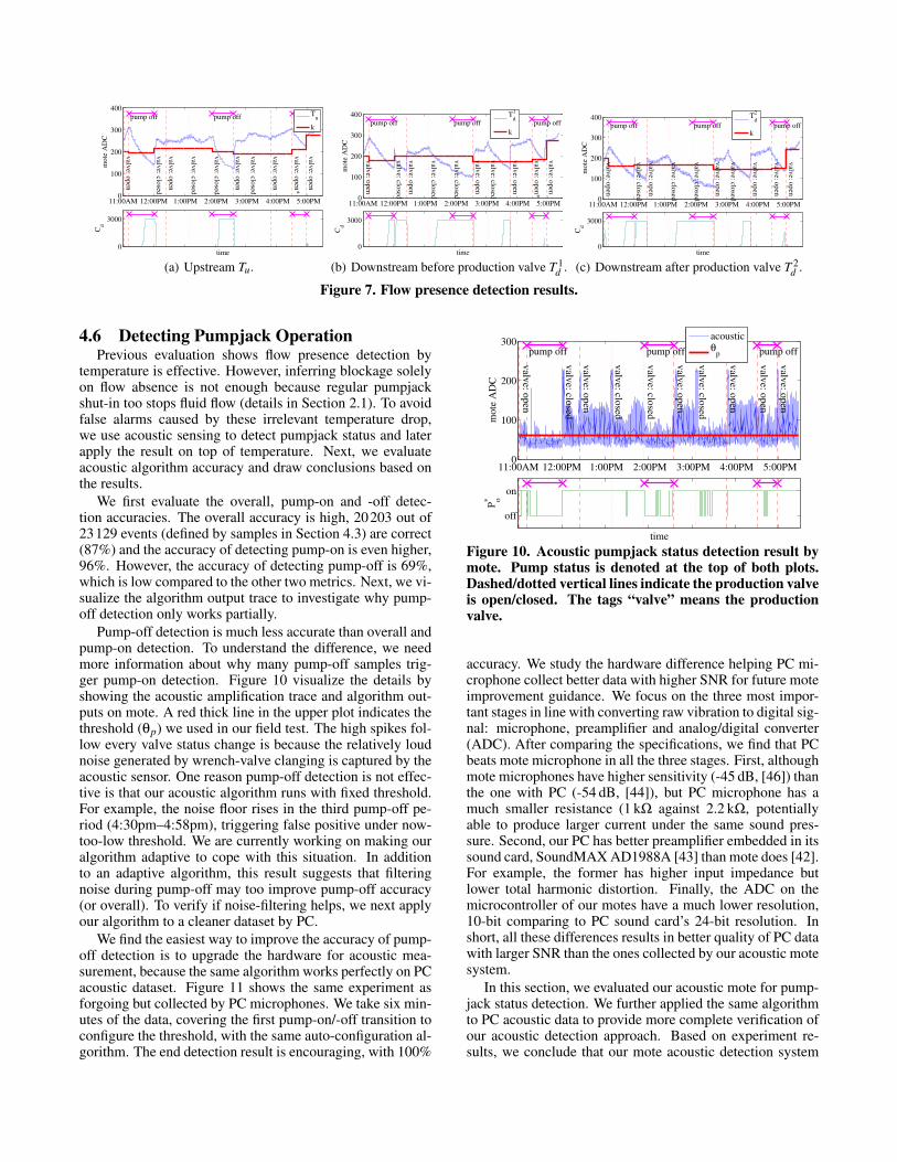
The three plots in Figure 7 shows that our CUSUM-based,flow presence detection algorithm works perfectly during ourfield test. We achieve 100% accuracy for the all ten eventswithout any false positive or negative and we discuss moredetailed observation below. Since Tu is upstream to both pro-duction and circulation valves, oil flows as long as pumpjackis on, regardless the status of the production valve. Fig-ure 7(a) shows our algorithm remains silent while pump ison and temperature drops upon the first two pump-off eventseffectively triggers our algorithm. In addition, our algorithmsuccessfully detects temperature drop caused by in-line valveclose-up, showing in Figure 7(b) and 7(c), where Cd buildsup at all “valve:closed” events.

We expect to see a trigger in the third pump-off event(4:30pm–4:58pm, marked “*”), but surprisingly Cd does notbuild up high enough in the algorithm, different from theprior two pump-off events. We still count that a true posi-tive rather than a false negative, because it is a result of ourcompressed experimental schedule—we ran out of the timeat the end of our experiment and hence we cut-off the thirdpump-off event prematurely. The trend shows we require 5

0

100

200

300

400

TuT

1

dT

2

d

all data

mote

AD

C

TuT

1

dT

2

d

normal flow only

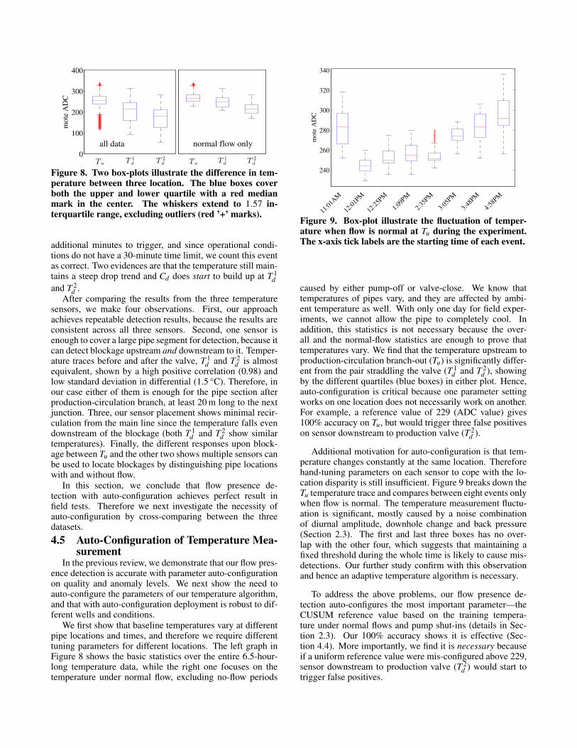
Figure 8. Two box-plots illustrate the difference in tem-perature between three location. The blue boxes coverboth the upper and lower quartile with a red medianmark in the center. The whiskers extend to 1.57 in-terquartile range, excluding outliers (red ’+’ marks).

additional minutes to trigger, and since operational condi-tions do not have a 30-minute time limit, we count this eventas correct. Two evidences are that the temperature still main-tains a steep drop trend and Cd does start to build up at T 1

d

and T 2d .

After comparing the results from the three temperaturesensors, we make four observations. First, our approachachieves repeatable detection results, because the results areconsistent across all three sensors. Second, one sensor isenough to cover a large pipe segment for detection, because itcan detect blockage upstream and downstream to it. Temper-ature traces before and after the valve, T 1

d and T 2d is almost

equivalent, shown by a high positive correlation (0.98) andlow standard deviation in differential (1.5 °C). Therefore, inour case either of them is enough for the pipe section afterproduction-circulation branch, at least 20 m long to the nextjunction. Three, our sensor placement shows minimal recir-culation from the main line since the temperature falls evendownstream of the blockage (both T 1

d and T 2d show similar

temperatures). Finally, the different responses upon block-age between Tu and the other two shows multiple sensors canbe used to locate blockages by distinguishing pipe locationswith and without flow.

In this section, we conclude that flow presence de-tection with auto-configuration achieves perfect result infield tests. Therefore we next investigate the necessity ofauto-configuration by cross-comparing between the threedatasets.

4.5 Auto-Configuration of Temperature Mea-surement

In the previous review, we demonstrate that our flow pres-ence detection is accurate with parameter auto-configurationon quality and anomaly levels. We next show the need toauto-configure the parameters of our temperature algorithm,and that with auto-configuration deployment is robust to dif-ferent wells and conditions.

We first show that baseline temperatures vary at differentpipe locations and times, and therefore we require differenttuning parameters for different locations. The left graph inFigure 8 shows the basic statistics over the entire 6.5-hour-long temperature data, while the right one focuses on thetemperature under normal flow, excluding no-flow periods

240

260

280

300

320

340

11:0

1AM

12:0

1PM

12:2

5PM

1:09

PM

2:35

PM

3:05

PM

3:48

PM

4:58

PM

mo

te A

DC

Figure 9. Box-plot illustrate the fluctuation of temper-ature when flow is normal at Tu during the experiment.The x-axis tick labels are the starting time of each event.

caused by either pump-off or valve-close. We know thattemperatures of pipes vary, and they are affected by ambi-ent temperature as well. With only one day for field exper-iments, we cannot allow the pipe to completely cool. Inaddition, this statistics is not necessary because the over-all and the normal-flow statistics are enough to prove thattemperatures vary. We find that the temperature upstream toproduction-circulation branch-out (Tu) is significantly differ-ent from the pair straddling the valve (T 1

d and T 2d ), showing

by the different quartiles (blue boxes) in either plot. Hence,auto-configuration is critical because one parameter settingworks on one location does not necessarily work on another.For example, a reference value of 229 (ADC value) gives100% accuracy on Tu, but would trigger three false positiveson sensor downstream to production valve (T 2

d ).

Additional motivation for auto-configuration is that tem-perature changes constantly at the same location. Thereforehand-tuning parameters on each sensor to cope with the lo-cation disparity is still insufficient. Figure 9 breaks down theTu temperature trace and compares between eight events onlywhen flow is normal. The temperature measurement fluctu-ation is significant, mostly caused by a noise combinationof diurnal amplitude, downhole change and back pressure(Section 2.3). The first and last three boxes has no over-lap with the other four, which suggests that maintaining afixed threshold during the whole time is likely to cause mis-detections. Our further study confirm with this observationand hence an adaptive temperature algorithm is necessary.

To address the above problems, our flow presence de-tection auto-configures the most important parameter—theCUSUM reference value based on the training tempera-ture under normal flows and pump shut-ins (details in Sec-tion 2.3). Our 100% accuracy shows it is effective (Sec-tion 4.4). More importantly, we find it is necessary becauseif a uniform reference value were mis-configured above 229,sensor downstream to production valve (T 2

d ) would start totrigger false positives.

11:00AM 12:00PM 1:00PM 2:00PM 3:00PM 4:00PM 5:00PM0

100

200

300

400

valv

e: closed

valv

e: closed

valv

e: closed

valv

e: closed

valv

e: op

en

valv

e: op

en

valv

e: op

en

valv

e: op

en

valv

e: op

en*

valv

e: op

en

pump off pump off pump off

mo

te A

DC

0

3000

Cd

time

Tu

k

(a) Upstream Tu.

11:00AM 12:00PM 1:00PM 2:00PM 3:00PM 4:00PM 5:00PM0

100

200

300

400

valv

e: closed

valv

e: closed

valv

e: closed

valv

e: closed

valv

e: op

en

valv

e: op

en

valv

e: op

en

valv

e: op

en

valv

e: op

en*

valv

e: op

en


mo

te A

DC

0

3000

Cd

time

Td

1

k

(b) Downstream before production valve T 1d .

11:00AM 12:00PM 1:00PM 2:00PM 3:00PM 4:00PM 5:00PM0

100

200

300

400

valv

e: closed

valv

e: closed

valv

e: closed

valv

e: closed

valv

e: op

en

valv

e: op

en

valv

e: op

en

valv

e: op

en

valv

e: op

en

valv

e: op

en


mo

te A

DC

0

3000

Cd

time

Td

2

k

(c) Downstream after production valve T 2d .

Figure 7. Flow presence detection results.

4.6 Detecting Pumpjack OperationPrevious evaluation shows flow presence detection by

temperature is effective. However, inferring blockage solelyon flow absence is not enough because regular pumpjackshut-in too stops fluid flow (details in Section 2.1). To avoidfalse alarms caused by these irrelevant temperature drop,we use acoustic sensing to detect pumpjack status and laterapply the result on top of temperature. Next, we evaluateacoustic algorithm accuracy and draw conclusions based onthe results.

We first evaluate the overall, pump-on and -off detec-tion accuracies. The overall accuracy is high, 20203 out of23129 events (defined by samples in Section 4.3) are correct(87%) and the accuracy of detecting pump-on is even higher,96%. However, the accuracy of detecting pump-off is 69%,which is low compared to the other two metrics. Next, we vi-sualize the algorithm output trace to investigate why pump-off detection only works partially.

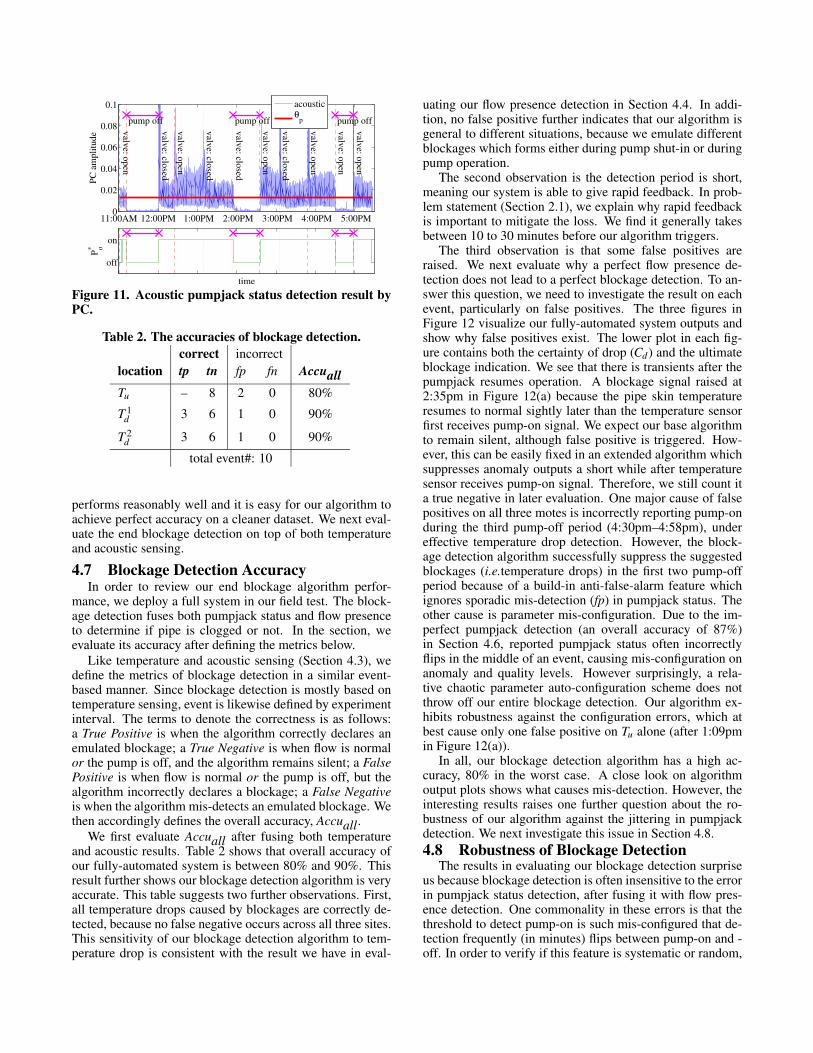
Pump-off detection is much less accurate than overall andpump-on detection. To understand the difference, we needmore information about why many pump-off samples trig-ger pump-on detection. Figure 10 visualize the details byshowing the acoustic amplification trace and algorithm out-puts on mote. A red thick line in the upper plot indicates thethreshold (θp) we used in our field test. The high spikes fol-low every valve status change is because the relatively loudnoise generated by wrench-valve clanging is captured by theacoustic sensor. One reason pump-off detection is not effec-tive is that our acoustic algorithm runs with fixed threshold.For example, the noise floor rises in the third pump-off pe-riod (4:30pm–4:58pm), triggering false positive under now-too-low threshold. We are currently working on making ouralgorithm adaptive to cope with this situation. In additionto an adaptive algorithm, this result suggests that filteringnoise during pump-off may too improve pump-off accuracy(or overall). To verify if noise-filtering helps, we next applyour algorithm to a cleaner dataset by PC.

We find the easiest way to improve the accuracy of pump-off detection is to upgrade the hardware for acoustic mea-surement, because the same algorithm works perfectly on PCacoustic dataset. Figure 11 shows the same experiment asforgoing but collected by PC microphones. We take six min-utes of the data, covering the first pump-on/-off transition toconfigure the threshold, with the same auto-configuration al-gorithm. The end detection result is encouraging, with 100%

11:00AM 12:00PM 1:00PM 2:00PM 3:00PM 4:00PM 5:00PM0

100

200

300

valv

e: closed

valv

e: closed

valv

e: closed

valv

e: closed

valv

e: open

valv

e: open

valv

e: open

valv

e: open

valv

e: open

valv

e: open


mote

AD

C

off

onP

o*

time

acousticθ

p

Figure 10. Acoustic pumpjack status detection result bymote. Pump status is denoted at the top of both plots.Dashed/dotted vertical lines indicate the production valveis open/closed. The tags “valve” means the productionvalve.

accuracy. We study the hardware difference helping PC mi-crophone collect better data with higher SNR for future moteimprovement guidance. We focus on the three most impor-tant stages in line with converting raw vibration to digital sig-nal: microphone, preamplifier and analog/digital converter(ADC). After comparing the specifications, we find that PCbeats mote microphone in all the three stages. First, althoughmote microphones have higher sensitivity (-45 dB, [46]) thanthe one with PC (-54 dB, [44]), but PC microphone has amuch smaller resistance (1 kΩ against 2.2 kΩ, potentiallyable to produce larger current under the same sound pres-sure. Second, our PC has better preamplifier embedded in itssound card, SoundMAX AD1988A [43] than mote does [42].For example, the former has higher input impedance butlower total harmonic distortion. Finally, the ADC on themicrocontroller of our motes have a much lower resolution,10-bit comparing to PC sound card’s 24-bit resolution. Inshort, all these differences results in better quality of PC datawith larger SNR than the ones collected by our acoustic motesystem.

In this section, we evaluated our acoustic mote for pump-jack status detection. We further applied the same algorithmto PC acoustic data to provide more complete verification ofour acoustic detection approach. Based on experiment re-sults, we conclude that our mote acoustic detection system

11:00AM 12:00PM 1:00PM 2:00PM 3:00PM 4:00PM 5:00PM0

0.02

0.04

0.06

0.08

0.1

valv

e: closed

valv

e: closed

valv

e: closed

valv

e: closed

valv

e: open

valv

e: open

valv

e: open

valv

e: open

valv

e: open

valv

e: open


PC

am

pli

tude

off

on

Po*

time

acousticθ

p

Figure 11. Acoustic pumpjack status detection result byPC.

Table 2. The accuracies of blockage detection.

correct incorrect

location tp tn fp fn Accuall

Tu – 8 2 0 80%

T 1d 3 6 1 0 90%

T 2d 3 6 1 0 90%

total event#: 10

performs reasonably well and it is easy for our algorithm toachieve perfect accuracy on a cleaner dataset. We next eval-uate the end blockage detection on top of both temperatureand acoustic sensing.

4.7 Blockage Detection AccuracyIn order to review our end blockage algorithm perfor-

mance, we deploy a full system in our field test. The block-age detection fuses both pumpjack status and flow presenceto determine if pipe is clogged or not. In the section, weevaluate its accuracy after defining the metrics below.

Like temperature and acoustic sensing (Section 4.3), wedefine the metrics of blockage detection in a similar event-based manner. Since blockage detection is mostly based ontemperature sensing, event is likewise defined by experimentinterval. The terms to denote the correctness is as follows:a True Positive is when the algorithm correctly declares anemulated blockage; a True Negative is when flow is normalor the pump is off, and the algorithm remains silent; a FalsePositive is when flow is normal or the pump is off, but thealgorithm incorrectly declares a blockage; a False Negativeis when the algorithm mis-detects an emulated blockage. Wethen accordingly defines the overall accuracy, Accuall.

We first evaluate Accuall after fusing both temperatureand acoustic results. Table 2 shows that overall accuracy ofour fully-automated system is between 80% and 90%. Thisresult further shows our blockage detection algorithm is veryaccurate. This table suggests two further observations. First,all temperature drops caused by blockages are correctly de-tected, because no false negative occurs across all three sites.This sensitivity of our blockage detection algorithm to tem-perature drop is consistent with the result we have in eval-

uating our flow presence detection in Section 4.4. In addi-tion, no false positive further indicates that our algorithm isgeneral to different situations, because we emulate differentblockages which forms either during pump shut-in or duringpump operation.

The second observation is the detection period is short,meaning our system is able to give rapid feedback. In prob-lem statement (Section 2.1), we explain why rapid feedbackis important to mitigate the loss. We find it generally takesbetween 10 to 30 minutes before our algorithm triggers.

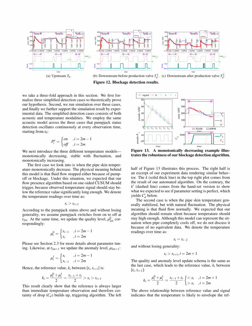
The third observation is that some false positives areraised. We next evaluate why a perfect flow presence de-tection does not lead to a perfect blockage detection. To an-swer this question, we need to investigate the result on eachevent, particularly on false positives. The three figures inFigure 12 visualize our fully-automated system outputs andshow why false positives exist. The lower plot in each fig-ure contains both the certainty of drop (Cd) and the ultimateblockage indication. We see that there is transients after thepumpjack resumes operation. A blockage signal raised at2:35pm in Figure 12(a) because the pipe skin temperatureresumes to normal sightly later than the temperature sensorfirst receives pump-on signal. We expect our base algorithmto remain silent, although false positive is triggered. How-ever, this can be easily fixed in an extended algorithm whichsuppresses anomaly outputs a short while after temperaturesensor receives pump-on signal. Therefore, we still count ita true negative in later evaluation. One major cause of falsepositives on all three motes is incorrectly reporting pump-onduring the third pump-off period (4:30pm–4:58pm), undereffective temperature drop detection. However, the block-age detection algorithm successfully suppress the suggestedblockages (i.e.temperature drops) in the first two pump-offperiod because of a build-in anti-false-alarm feature whichignores sporadic mis-detection (fp) in pumpjack status. Theother cause is parameter mis-configuration. Due to the im-perfect pumpjack detection (an overall accuracy of 87%)in Section 4.6, reported pumpjack status often incorrectlyflips in the middle of an event, causing mis-configuration onanomaly and quality levels. However surprisingly, a rela-tive chaotic parameter auto-configuration scheme does notthrow off our entire blockage detection. Our algorithm ex-hibits robustness against the configuration errors, which atbest cause only one false positive on Tu alone (after 1:09pmin Figure 12(a)).

In all, our blockage detection algorithm has a high ac-curacy, 80% in the worst case. A close look on algorithmoutput plots shows what causes mis-detection. However, theinteresting results raises one further question about the ro-bustness of our algorithm against the jittering in pumpjackdetection. We next investigate this issue in Section 4.8.

4.8 Robustness of Blockage DetectionThe results in evaluating our blockage detection surprise

us because blockage detection is often insensitive to the errorin pumpjack status detection, after fusing it with flow pres-ence detection. One commonality in these errors is that thethreshold to detect pump-on is such mis-configured that de-tection frequently (in minutes) flips between pump-on and -off. In order to verify if this feature is systematic or random,

11:00AM 12:00PM 1:00PM 2:00PM 3:00PM 4:00PM 5:00PM0

100

200

300

400

valv

e: closed

valv

e: closed

valv

e: closed

valv

e: closed

valv

e: op

en

valv

e: op

en

valv

e: op

en

valv

e: op

en

valv

e: op

en

valv

e: op

en


mo

te A

DC

T

u

k

false

true

blo

ck.

.

time

0

3000

.

C

d

(a) Upstream Tu.

11:00AM 12:00PM 1:00PM 2:00PM 3:00PM 4:00PM 5:00PM0

100

200

300

400

valv

e: closed

valv

e: closed

valv

e: closed

valv

e: closed

valv

e: op

en

valv

e: op

en

valv

e: op

en

valv

e: op

en

valv

e: op

en

valv

e: op

en


mo

te A

DC

Td

1

k

false

true

blo

ck.

.

time

0

3000

.

C

d

(b) Downstream before production valve T 1d .

11:00AM 12:00PM 1:00PM 2:00PM 3:00PM 4:00PM 5:00PM0

100

200

300

400

valv

e: closed

valv

e: closed

valv

e: closed

valv

e: closed

valv

e: op

en

valv

e: op

en

valv

e: op

en

valv

e: op

en

valv

e: op

en

valv

e: op

en


mo

te A

DC

Td

2

k

false

true

blo

ck.

.

time

0

3000

.

C

d

(c) Downstream after production valve T 2d .

Figure 12. Blockage detection results.

we take a three-fold approach in this section. We first for-malize three simplified detection cases to theoretically proveour hypothesis. Second, we run simulation over these cases,and finally we further support the simulation result by exper-imental data. The simplified detection cases consists of bothacoustic and temperature modalities. We employ the sameacoustic model across the three cases that pumpjack statusdetection oscillates continuously at every observation time,starting from t0:

Poi =

on , i = 2m−1

off , i = 2m

We next introduce the three different temperature models—monotonically decreasing, stable with fluctuation, andmonotonically increasing.

The first case we look into is when the pipe skin temper-ature monotonically decrease. The physical meaning behindthis model is that fluid flow stopped either because of pump-off or blockage. Under this situation, we expected that ourflow presence algorithm based on one-sided CUSUM shouldtrigger, because observed temperature signal should stay be-low the reference value significantly long enough. We denotethe temperature readings over time as:

si > si+1

According to the pumpjack status above and without losinggenerality, we assume pumpjack switches from on to off att2m. At the same time, we update the quality level, µ0

2m cor-respondingly:

µ0i =

si−1 , i = 2m−1

si , i = 2m

Please see Section 2.3 for more details about parameter tun-ing. Likewise, at t2m+1 we update the anomaly level, µ2m+1:

µ1i =

si , i = 2m−1

si−1 , i = 2m

Hence, the reference value, ki between [ti, ti+1] is:

ki =µ0

i +µ1i

2=

si−1 + si

2> si > si+1

This result clearly show that the reference is always largerthan immediate temperature observation and therefore cer-tainty of drop (Cd) builds up, triggering algorithm. The left

0

20

40

60

80

t0 t1 t2 t3 t4 t5 t6 t7

pse

ud

o-A

DC

signal km

0m

1

off

onp

seu

do

-Po

time

11:30AM 12:00PM0

100

200

300

400

mo

te A

DC

time

0

3000

Cd

time

Td

1

k

k’

Cd

Cd’

Figure 13. A monotonically decreasing example illus-trates the robustness of our blockage detection algorithm.

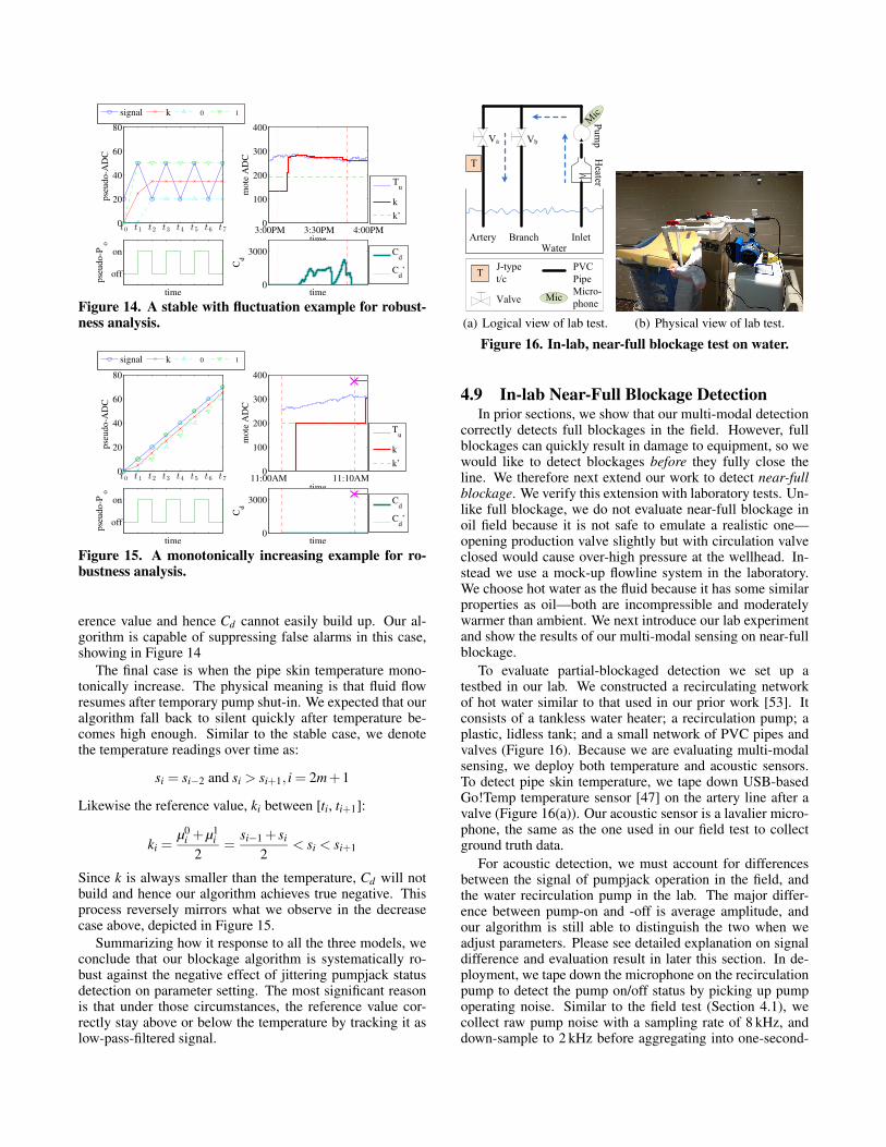
half of Figure 13 illustrates this process. The right half isan excerpt of our experiment data rendering similar behav-ior. The k (solid thick line) in the top right plot comes fromthe result of our automated algorithm. On the contrary, thek′ (dashed line) comes from the hand-set version to showwhat we expected to see if parameter setting is perfect, whichyields C′

d below.The second case is when the pipe skin temperature gen-

erally stabilized, but with natural fluctuation. The physicalmeaning is that fluid flow normally. We expected that ouralgorithm should remain silent because temperature shouldstay high enough. Although this model can represent the sit-uation when pipe completely cools off, we do not discuss itbecause of no equivalent data. We denote the temperaturereadings over time as:

si = si−2

and without losing generality:

si > si+1, i = 2m+1

The quality and anomaly level update schema is the same asthe last case, which leads to the reference value, ki between[ti, ti+1]:

ki =µ0

i +µ1i

2=

si−1 + si

2

< si , i = 2m+1

> si , i = 2m

The above relationship between reference value and signalindicates that the temperature is likely to envelope the ref-

0

20

40

60

80

t0 t1 t2 t3 t4 t5 t6 t7

pse

udo-A

DC

signal km

0m

1

off

on

pse

udo-P

o

time

3:00PM 3:30PM 4:00PM0

100

200

300

400

mote

AD

Ctime

0

3000

Cd

time

Tu

k

k’

Cd

Cd’

Figure 14. A stable with fluctuation example for robust-ness analysis.

0

20

40

60

80

t0 t1 t2 t3 t4 t5 t6 t7

pse

udo-A

DC

signal km

0m

1

off

on

pse

udo-P

o

time

11:00AM 11:10AM0

100

200

300

400

mote

AD

C

time

0

3000

Cd

time

Tu

k

k’

Cd

Cd’

Figure 15. A monotonically increasing example for ro-bustness analysis.

erence value and hence Cd cannot easily build up. Our al-gorithm is capable of suppressing false alarms in this case,showing in Figure 14

The final case is when the pipe skin temperature mono-tonically increase. The physical meaning is that fluid flowresumes after temporary pump shut-in. We expected that ouralgorithm fall back to silent quickly after temperature be-comes high enough. Similar to the stable case, we denotethe temperature readings over time as:

si = si−2 and si > si+1, i = 2m+1

Likewise the reference value, ki between [ti, ti+1]:

ki =µ0

i +µ1i

2=

si−1 + si

2< si < si+1

Since k is always smaller than the temperature, Cd will notbuild and hence our algorithm achieves true negative. Thisprocess reversely mirrors what we observe in the decreasecase above, depicted in Figure 15.

Summarizing how it response to all the three models, weconclude that our blockage algorithm is systematically ro-bust against the negative effect of jittering pumpjack statusdetection on parameter setting. The most significant reasonis that under those circumstances, the reference value cor-rectly stay above or below the temperature by tracking it aslow-pass-filtered signal.

!

" #

#

(a) Logical view of lab test. (b) Physical view of lab test.

Figure 16. In-lab, near-full blockage test on water.

4.9 In-lab Near-Full Blockage DetectionIn prior sections, we show that our multi-modal detection

correctly detects full blockages in the field. However, fullblockages can quickly result in damage to equipment, so wewould like to detect blockages before they fully close theline. We therefore next extend our work to detect near-fullblockage. We verify this extension with laboratory tests. Un-like full blockage, we do not evaluate near-full blockage inoil field because it is not safe to emulate a realistic one—opening production valve slightly but with circulation valveclosed would cause over-high pressure at the wellhead. In-stead we use a mock-up flowline system in the laboratory.We choose hot water as the fluid because it has some similarproperties as oil—both are incompressible and moderatelywarmer than ambient. We next introduce our lab experimentand show the results of our multi-modal sensing on near-fullblockage.

To evaluate partial-blockaged detection we set up atestbed in our lab. We constructed a recirculating networkof hot water similar to that used in our prior work [53]. Itconsists of a tankless water heater; a recirculation pump; aplastic, lidless tank; and a small network of PVC pipes andvalves (Figure 16). Because we are evaluating multi-modalsensing, we deploy both temperature and acoustic sensors.To detect pipe skin temperature, we tape down USB-basedGo!Temp temperature sensor [47] on the artery line after avalve (Figure 16(a)). Our acoustic sensor is a lavalier micro-phone, the same as the one used in our field test to collectground truth data.

For acoustic detection, we must account for differencesbetween the signal of pumpjack operation in the field, andthe water recirculation pump in the lab. The major differ-ence between pump-on and -off is average amplitude, andour algorithm is still able to distinguish the two when weadjust parameters. Please see detailed explanation on signaldifference and evaluation result in later this section. In de-ployment, we tape down the microphone on the recirculationpump to detect the pump on/off status by picking up pumpoperating noise. Similar to the field test (Section 4.1), wecollect raw pump noise with a sampling rate of 8 kHz, anddown-sample to 2 kHz before aggregating into one-second-

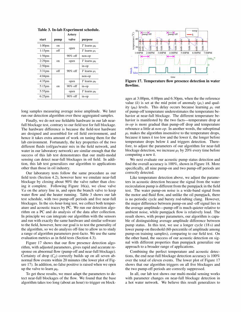
Table 3. In-lab Experiment schedule.

Artery

start pump valve purpose

1:00pm onopen

T learns µ0

1:15pm off T learns µ1

1:56pm

on

90% off non-op

2:29pm open T learns µ0

2:50pm

90% off

in-op

3:31pm off T learns µ1

4:04pm

on

non-op


5:15pm 90% off in-op


6:25pm 90% off in-op

long samples measuring average noise amplitude. We laterrun our detection algorithm over these aggregated samples.

Finally, we do not use fieldable hardware in our lab near-full blockage test, contrary to our field test for full blockage.The hardware difference is because the field-test hardwareare designed and assembled for oil field environment, andhence it takes extra amount of work on tuning them for thelab environment. Fortunately, the key properties of the twodifferent fluids (oil/gas/water mix in the field network, andwater in our laboratory network) are similar enough that thesuccess of this lab test demonstrates that our multi-modalsensing can detect near-full blockages in oil field. In addi-tion, this lab test generalizes our algorithm to applicationsother than those in oil industry.

Our laboratory tests follow the same procedure as ourfield tests (Section 4.2), however here we emulate near-fullblockage by closing about 90% the valve rather than clos-ing it complete. Following Figure 16(a), we close valveV.a on the artery line in, and open the branch valve to keepwater flow and the heater running. Table 3 shows our labtest schedule, with two pump-off periods and five near-fullblockages. In the six-hour-long test, we collect both temper-ature and acoustic traces by PC. We run our detection algo-rithm on a PC and do analysis of the data after collection.In principle we can integrate our algorithm with the sensorsand run with exactly the same hardware and similar softwareto the field, however, here our goal is to test the generality ofthe algorithm, so we do analysis off-line to allow us to studya range of algorithm parameters post-facto. We use the sameevaluation metrics as in field tests (Section 4.3).

Figure 17 shows that our flow presence detection algo-rithm, with adjusted parameters, gives rapid and accurate re-sponse on abnormal flow (pump-off and near-full blockage).Certainty of drop (Cd) correctly builds up on all seven ab-normal flow events within 20 minutes (the lower plot of Fig-ure 17). In addition, no false positive is raised when we openup the valve to learn µ0.

To get these results, we must adapt the parameters to de-tect near-full blockages of the flow. We found that the basealgorithm takes too long (about an hour) to trigger on block-

1:00PM 2:00PM 3:00PM 4:00PM 5:00PM 6:00PM 7:00PM

30

40

50

valv

e: 90%

valv

e: 90%

valv

e: 90%

valv

e: 90%

valv

e: 90%

valv

e: 90%

valv

e: open

valv

e: open

valv

e: open

valv

e: open

valv

e: open

pump off pump off

tem

per

ature

(oC

)

temp

k

false

true

blo

ck. .

time

0

500

. C

d

Figure 17. Temperature flow presence detection in waterflowline.

ages at 3:00pm, 4:00pm and 6:30pm, when the the referencevalue (k) is set at the mid point of anomaly (µ1) and qual-ity (µ0) levels. This delay occurs because learning µ1 outof pump-off temperature underestimates the temperature be-havior at near-full blockage. The different temperature be-havior is manifested by the two facts—temperature drop atin-op is more gradual than pump-off drop and temperaturerebounce a little at non-op. In another words, the suboptimalµ1 makes the algorithm insensitive to the temperature drops,because it tunes k too low and the lower k, the longer beforetemperature drops below k and triggers detection. There-fore, to adjust the parameters of our algorithm for near-fullblockage detection, we increase µ1 by 20% every time beforecomputing a new k.

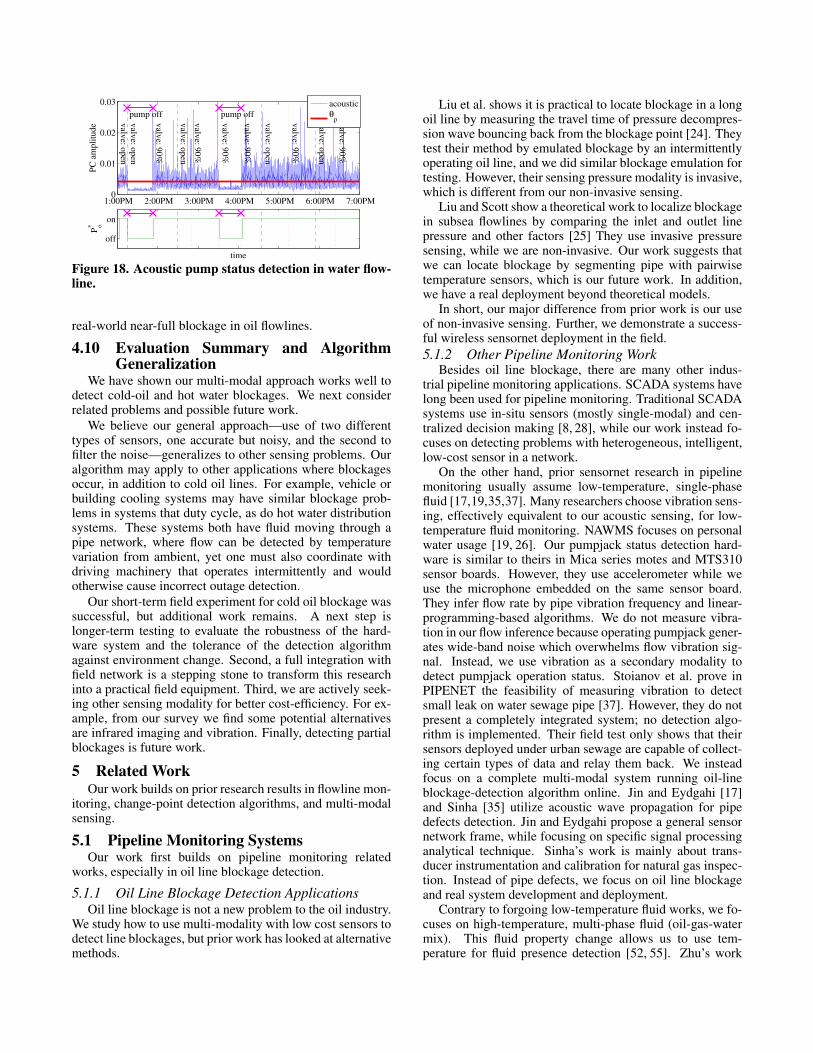
We next evaluate our acoustic pump status detection andfind the overall accuracy is 100%, shown in Figure 18. Morespecifically, all nine pump-on and two pump-off periods arecorrectly detected.

Like temperature detection above, we adjust the parame-ters in acoustic detection because the signal from the waterrecirculation pump is different from the pumpjack in the fieldtest. The water pump-on noise is a wide-band signal fromthe motor and fluid flow, and unlike the oil pumpjack, thereis no periodic cycle and bursty rod-tubing clang. However,the major difference between pump-on and -off signal lies inthe average amplitude—pump-off is much quieter relative toambient noise, while pumpjack flow is relatively loud. Theresult shows, with proper parameters, our algorithm is capa-ble of distinguishing average amplitude difference betweenpump status. In this test, we use a longer cycle (18 s) andlower pump-on threshold (60-percentile of amplitude amongpump-on training samples), comparing to our field test. Onthe other hand, the success of our acoustic detection on sig-nal with different properties than pumpjack generalize ourapproach to a broader range of applications.

Combining the perfect temperature and acoustic detec-tions, the end near-full blockage detection accuracy is 100%over the total of eleven events. The lower plot of Figure 17shows that our algorithm triggers on all five blockages andthe two pump-off periods are correctly suppressed.

In all, our lab test shows our multi-modal sensing workswith parameter changes on near-full blockage detection ina hot water network. We believe this result generalizes to

1:00PM 2:00PM 3:00PM 4:00PM 5:00PM 6:00PM 7:00PM0

0.01

0.02

0.03

valv

e: 90%

valv

e: 90%

valv

e: 90%

valv

e: 90%

valv

e: 90%

valv

e: 90%

valv

e: open

valv

e: open

valv

e: open

valv

e: open

valv

e: open

pump off pump off

PC

am

pli

tude

off

on

Po*

time

acoustic

θp

Figure 18. Acoustic pump status detection in water flow-line.

real-world near-full blockage in oil flowlines.

4.10 Evaluation Summary and AlgorithmGeneralization

We have shown our multi-modal approach works well todetect cold-oil and hot water blockages. We next considerrelated problems and possible future work.

We believe our general approach—use of two differenttypes of sensors, one accurate but noisy, and the second tofilter the noise—generalizes to other sensing problems. Ouralgorithm may apply to other applications where blockagesoccur, in addition to cold oil lines. For example, vehicle orbuilding cooling systems may have similar blockage prob-lems in systems that duty cycle, as do hot water distributionsystems. These systems both have fluid moving through apipe network, where flow can be detected by temperaturevariation from ambient, yet one must also coordinate withdriving machinery that operates intermittently and wouldotherwise cause incorrect outage detection.

Our short-term field experiment for cold oil blockage wassuccessful, but additional work remains. A next step islonger-term testing to evaluate the robustness of the hard-ware system and the tolerance of the detection algorithmagainst environment change. Second, a full integration withfield network is a stepping stone to transform this researchinto a practical field equipment. Third, we are actively seek-ing other sensing modality for better cost-efficiency. For ex-ample, from our survey we find some potential alternativesare infrared imaging and vibration. Finally, detecting partialblockages is future work.

5 Related WorkOur work builds on prior research results in flowline mon-

itoring, change-point detection algorithms, and multi-modalsensing.

5.1 Pipeline Monitoring SystemsOur work first builds on pipeline monitoring related

works, especially in oil line blockage detection.

5.1.1 Oil Line Blockage Detection ApplicationsOil line blockage is not a new problem to the oil industry.

We study how to use multi-modality with low cost sensors todetect line blockages, but prior work has looked at alternativemethods.

Liu et al. shows it is practical to locate blockage in a longoil line by measuring the travel time of pressure decompres-sion wave bouncing back from the blockage point [24]. Theytest their method by emulated blockage by an intermittentlyoperating oil line, and we did similar blockage emulation fortesting. However, their sensing pressure modality is invasive,which is different from our non-invasive sensing.

Liu and Scott show a theoretical work to localize blockagein subsea flowlines by comparing the inlet and outlet linepressure and other factors [25] They use invasive pressuresensing, while we are non-invasive. Our work suggests thatwe can locate blockage by segmenting pipe with pairwisetemperature sensors, which is our future work. In addition,we have a real deployment beyond theoretical models.

In short, our major difference from prior work is our useof non-invasive sensing. Further, we demonstrate a success-ful wireless sensornet deployment in the field.

5.1.2 Other Pipeline Monitoring WorkBesides oil line blockage, there are many other indus-

trial pipeline monitoring applications. SCADA systems havelong been used for pipeline monitoring. Traditional SCADAsystems use in-situ sensors (mostly single-modal) and cen-tralized decision making [8, 28], while our work instead fo-cuses on detecting problems with heterogeneous, intelligent,low-cost sensor in a network.

On the other hand, prior sensornet research in pipelinemonitoring usually assume low-temperature, single-phasefluid [17,19,35,37]. Many researchers choose vibration sens-ing, effectively equivalent to our acoustic sensing, for low-temperature fluid monitoring. NAWMS focuses on personalwater usage [19, 26]. Our pumpjack status detection hard-ware is similar to theirs in Mica series motes and MTS310sensor boards. However, they use accelerometer while weuse the microphone embedded on the same sensor board.They infer flow rate by pipe vibration frequency and linear-programming-based algorithms. We do not measure vibra-tion in our flow inference because operating pumpjack gener-ates wide-band noise which overwhelms flow vibration sig-nal. Instead, we use vibration as a secondary modality todetect pumpjack operation status. Stoianov et al. prove inPIPENET the feasibility of measuring vibration to detectsmall leak on water sewage pipe [37]. However, they do notpresent a completely integrated system; no detection algo-rithm is implemented. Their field test only shows that theirsensors deployed under urban sewage are capable of collect-ing certain types of data and relay them back. We insteadfocus on a complete multi-modal system running oil-lineblockage-detection algorithm online. Jin and Eydgahi [17]and Sinha [35] utilize acoustic wave propagation for pipedefects detection. Jin and Eydgahi propose a general sensornetwork frame, while focusing on specific signal processinganalytical technique. Sinha’s work is mainly about trans-ducer instrumentation and calibration for natural gas inspec-tion. Instead of pipe defects, we focus on oil line blockageand real system development and deployment.

Contrary to forgoing low-temperature fluid works, we fo-cuses on high-temperature, multi-phase fluid (oil-gas-watermix). This fluid property change allows us to use tem-perature for fluid presence detection [52, 55]. Zhu’s work

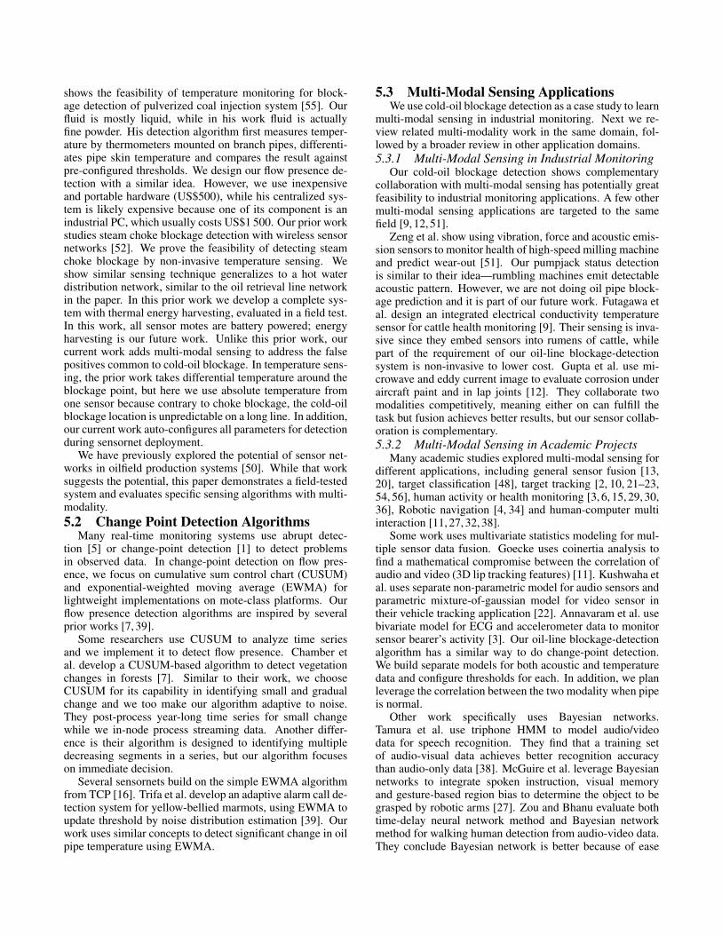
shows the feasibility of temperature monitoring for block-age detection of pulverized coal injection system [55]. Ourfluid is mostly liquid, while in his work fluid is actuallyfine powder. His detection algorithm first measures temper-ature by thermometers mounted on branch pipes, differenti-ates pipe skin temperature and compares the result againstpre-configured thresholds. We design our flow presence de-tection with a similar idea. However, we use inexpensiveand portable hardware (US$500), while his centralized sys-tem is likely expensive because one of its component is anindustrial PC, which usually costs US$1 500. Our prior workstudies steam choke blockage detection with wireless sensornetworks [52]. We prove the feasibility of detecting steamchoke blockage by non-invasive temperature sensing. Weshow similar sensing technique generalizes to a hot waterdistribution network, similar to the oil retrieval line networkin the paper. In this prior work we develop a complete sys-tem with thermal energy harvesting, evaluated in a field test.In this work, all sensor motes are battery powered; energyharvesting is our future work. Unlike this prior work, ourcurrent work adds multi-modal sensing to address the falsepositives common to cold-oil blockage. In temperature sens-ing, the prior work takes differential temperature around theblockage point, but here we use absolute temperature fromone sensor because contrary to choke blockage, the cold-oilblockage location is unpredictable on a long line. In addition,our current work auto-configures all parameters for detectionduring sensornet deployment.

We have previously explored the potential of sensor net-works in oilfield production systems [50]. While that worksuggests the potential, this paper demonstrates a field-testedsystem and evaluates specific sensing algorithms with multi-modality.

5.2 Change Point Detection AlgorithmsMany real-time monitoring systems use abrupt detec-

tion [5] or change-point detection [1] to detect problemsin observed data. In change-point detection on flow pres-ence, we focus on cumulative sum control chart (CUSUM)and exponential-weighted moving average (EWMA) forlightweight implementations on mote-class platforms. Ourflow presence detection algorithms are inspired by severalprior works [7, 39].

Some researchers use CUSUM to analyze time seriesand we implement it to detect flow presence. Chamber etal. develop a CUSUM-based algorithm to detect vegetationchanges in forests [7]. Similar to their work, we chooseCUSUM for its capability in identifying small and gradualchange and we too make our algorithm adaptive to noise.They post-process year-long time series for small changewhile we in-node process streaming data. Another differ-ence is their algorithm is designed to identifying multipledecreasing segments in a series, but our algorithm focuseson immediate decision.

Several sensornets build on the simple EWMA algorithmfrom TCP [16]. Trifa et al. develop an adaptive alarm call de-tection system for yellow-bellied marmots, using EWMA toupdate threshold by noise distribution estimation [39]. Ourwork uses similar concepts to detect significant change in oilpipe temperature using EWMA.

5.3 Multi-Modal Sensing ApplicationsWe use cold-oil blockage detection as a case study to learn

multi-modal sensing in industrial monitoring. Next we re-view related multi-modality work in the same domain, fol-lowed by a broader review in other application domains.

5.3.1 Multi-Modal Sensing in Industrial MonitoringOur cold-oil blockage detection shows complementary

collaboration with multi-modal sensing has potentially greatfeasibility to industrial monitoring applications. A few othermulti-modal sensing applications are targeted to the samefield [9, 12, 51].

Zeng et al. show using vibration, force and acoustic emis-sion sensors to monitor health of high-speed milling machineand predict wear-out [51]. Our pumpjack status detectionis similar to their idea—rumbling machines emit detectableacoustic pattern. However, we are not doing oil pipe block-age prediction and it is part of our future work. Futagawa etal. design an integrated electrical conductivity temperaturesensor for cattle health monitoring [9]. Their sensing is inva-sive since they embed sensors into rumens of cattle, whilepart of the requirement of our oil-line blockage-detectionsystem is non-invasive to lower cost. Gupta et al. use mi-crowave and eddy current image to evaluate corrosion underaircraft paint and in lap joints [12]. They collaborate twomodalities competitively, meaning either on can fulfill thetask but fusion achieves better results, but our sensor collab-oration is complementary.

5.3.2 Multi-Modal Sensing in Academic ProjectsMany academic studies explored multi-modal sensing for

different applications, including general sensor fusion [13,20], target classification [48], target tracking [2, 10, 21–23,54, 56], human activity or health monitoring [3, 6, 15, 29, 30,36], Robotic navigation [4, 34] and human-computer multiinteraction [11, 27, 32, 38].

Some work uses multivariate statistics modeling for mul-tiple sensor data fusion. Goecke uses coinertia analysis tofind a mathematical compromise between the correlation ofaudio and video (3D lip tracking features) [11]. Kushwaha etal. uses separate non-parametric model for audio sensors andparametric mixture-of-gaussian model for video sensor intheir vehicle tracking application [22]. Annavaram et al. usebivariate model for ECG and accelerometer data to monitorsensor bearer’s activity [3]. Our oil-line blockage-detectionalgorithm has a similar way to do change-point detection.We build separate models for both acoustic and temperaturedata and configure thresholds for each. In addition, we planleverage the correlation between the two modality when pipeis normal.

Other work specifically uses Bayesian networks.Tamura et al. use triphone HMM to model audio/videodata for speech recognition. They find that a training setof audio-visual data achieves better recognition accuracythan audio-only data [38]. McGuire et al. leverage Bayesiannetworks to integrate spoken instruction, visual memoryand gesture-based region bias to determine the object to begrasped by robotic arms [27]. Zou and Bhanu evaluate bothtime-delay neural network method and Bayesian networkmethod for walking human detection from audio-video data.They conclude Bayesian network is better because of ease

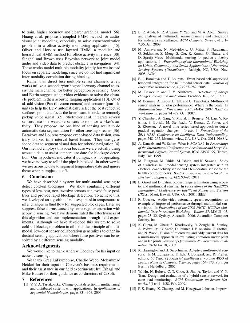
to train, higher accuracy and clearer graphical model [56].Huang et al. propose a coupled HMM method for audio-visual joint modeling, especially to solve asynchronizationproblem in a office activity monitoring application [15].Oliver and Horvitz use layered HMM, a modular andhierarchical HMM method for office activity inference [30].Singhal and Brown uses Bayesian network to joint modelaudio and video data to predict obstacle in navigation [34].These works model multiple modality jointly but we insteadfocus on separate modeling, since we do not find significantinter-modality correlation during blockage.

Rather than direct fuse multiple sensor channels, a fewworks utilize a secondary/orthogonal sensory channel to as-sist the main channel for better perception or sensing. Girodand Estrin suggest using video evidence to solve the obsta-cle problem in their acoustic ranging application [10]. Qu etal. add vision (Pan-tilt-zoom camera) and actuator (pan-tilt-unit) to help the LDV automatically select the best reflectivesurfaces, point and focus the laser beam, in order to remotelypickup voice signal [32]. Stiefmeier et al. integrate severalsensors into one wearable sensors to monitor worker’s ac-tivity. They propose use one kind of sensing result to doautomatic data segmentation for other sensing streams [36].Barakova and Lourens propose event-based data fusion, con-trary to fixed time interval based fusion. They use gyro-scope data to segment visual data for robotic navigation [4].Our method employs this idea because we are actually usingacoustic date to assist temperature date for blockage detec-tion. Our hypothesis indicates if pumpjack is not operating,we have no way to tell if the pipe is blocked. In other words,we use acoustic date to segment temperature date and ignorethose when pumpjack is off.

6 ConclusionWe have described a system for multi-modal sensing to

detect cold-oil blockages. We show combining differenttypes of low-cost, non-invasive sensors can avoid false posi-tives and provide rapid blockage detection. To achieve this,we developed an algorithm first uses pipe skin temperature toinfer changes in fluid flow for suggested blockages. Later wesuppress false alarms caused by some regular operation withacoustic sensing. We have demonstrated the effectiveness ofthis algorithm and our implementation through field exper-iments. Although we have developed this system to solvecold-oil blockage problem in oil field, the principle of multi-modal, low-cost sensor collaboration generalizes to other in-dustrial sensing applications where false positives can be re-solved by a different sensing modality.

AcknowledgmentsWe would like to thank Andrew Goodney for his input on

acoustic sensing.We thank Greg LaFramboise, Charlie Webb, Mohammad

Heidari for their input on Chevron’s business requirementsand their assistance in our field experiments; Iraj Erhagi andMike Hauser for their guidance as co-directors of CiSoft.

7 References[1] V. V. A. Tartakovsky. Change-point detection in multichannel

and distributed systems with applications. In Applications ofSequential Methodologies, pages 331–363, 2004.

[2] B. R. Abidi, N. R. Aragam, Y. Yao, and M. A. Abidi. Surveyand analysis of multimodal sensor planning and integrationfor wide area surveillance. ACM Computer Survey, 41:7:1–7:36, Jan. 2009.

[3] M. Annavaram, N. Medvidovic, U. Mitra, S. Narayanan,G. Sukhatme, Z. Meng, S. Qiu, R. Kumar, G. Thatte, andD. Spruijt-Metz. Multimodal sensing for pediatric obesityapplications. In Proceedings of the International Workshopon Urban, Community, and Social Applications of NetworkedSensing Systems (UrbanSense), Raleigh, NC, USA, Nov.2008. ACM.

[4] E. I. Barakova and T. Lourens. Event based self-supervisedtemporal integration for multimodal sensor data. Journal ofIntegrative Neuroscience, 4(2):265–282, 2005.

[5] M. Basseville and I. V. Nikiforov. Detection of abruptchanges: theory and application. Prentice-Hall, Inc., 1993.

[6] M. Benning, A. Kapur, B. Till, and G. Tzanetakis. Multimodalsensor analysis of sitar performance: Where is the beat? InMultimedia Signal Processing, 2007. MMSP 2007. IEEE 9thWorkshop on, pages 74 –77, Oct. 2007.

[7] Y. Chamber, A. Garg, V. Mithal, I. Brugere, M. Lau, V. Kr-ishna, S. Boriah, M. Steinbach, V. Kumar, C. Potter, andS. Klooster. A novel time series based approach to detectgradual vegetation changes in forests. In Proceedings of the2011 NASA Conference on Intelligent Data Understanding,pages 248–262, Mountainview, CA, USA, Oct. 2011. NASA.

[8] A. Daneels and W. Salter. What is SCADA? In Proceedingsof the International Conference on Accelerator and Large Ex-perimental Physics Control System, ICALEPCS ’99, Trieste,Italy, Oct. 1999.

[9] M. Futagawa, M. Ishida, M. Ishida, and K. Sawada. Studyof a wireless multimodal sensing system integrated with anelectrical conductivity sensor and a temperature sensor for thehealth control of cows. IEEE Transactions on Electrical andElectronic Engineering, 6(2):93–96, 2011.

[10] L. Girod and D. Estrin. Robust range estimation using acous-tic and multimodal sensing. In Proceedings of the IEEE/RSJInternational Conference on Intelligent Robots and Systems(IROS), Maui, Hawaii, USA, Oct. 2001. IEEE.

[11] R. Goecke. Audio-video automatic speech recognition: anexample of improved performance through multimodal sen-sor input. In Proceedings of the 2005 NICTA-HCSNet Mul-timodal User Interaction Workshop - Volume 57, MMUI ’05,pages 25–32, Sydney, Australia, 2006. Australian ComputerSociety, Inc.

[12] K. Gupta, M. Ghasr, S. Kharkovsky, R. Zoughi, R. Stanley,A. Padwal, M. O’Keefe, D. Palmer, J. Blackshire, G. Steffes,and N. Wood. Fusion of microwave and eddy current data fora multi-modal approach in evaluating corrosion under paintand in lap joints. Review of Quantitative Nondestructive Eval-uation, 26:611–618, 2007.

[13] K. Harrington and H. Siegelmann. Adaptive multi-modal sen-sors. In M. Lungarella, F. Iida, J. Bongard, and R. Pfeifer,editors, 50 Years of Artificial Intelligence, volume 4850 ofLecture Notes in Computer Science, pages 164–173. SpringerBerlin / Heidelberg, 2007.

[14] W. Hu, N. Bulusu, C. T. Chou, S. Jha, A. Taylor, and V. N.Tran. Design and evaluation of a hybrid sensor network forcane toad monitoring. ACM Transactions on Sensor Net-works, 5(1):4:1–4:28, Feb. 2009.

[15] P.-S. Huang, X. Zhuang, and M. Hasegawa-Johnson. Improv-

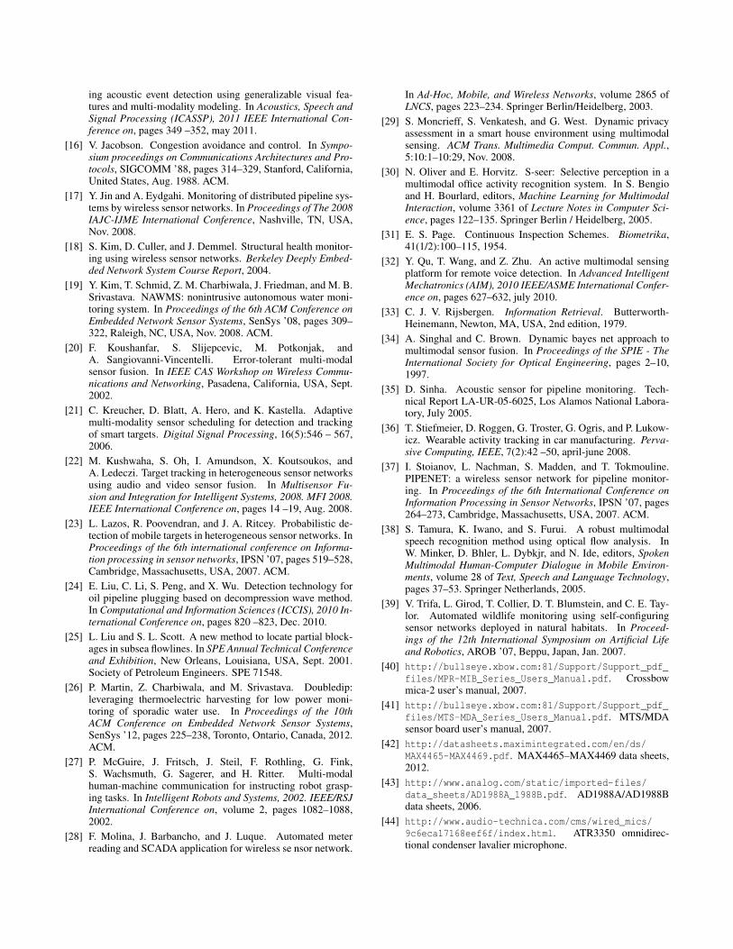
ing acoustic event detection using generalizable visual fea-tures and multi-modality modeling. In Acoustics, Speech andSignal Processing (ICASSP), 2011 IEEE International Con-ference on, pages 349 –352, may 2011.

[16] V. Jacobson. Congestion avoidance and control. In Sympo-sium proceedings on Communications Architectures and Pro-tocols, SIGCOMM ’88, pages 314–329, Stanford, California,United States, Aug. 1988. ACM.

[17] Y. Jin and A. Eydgahi. Monitoring of distributed pipeline sys-tems by wireless sensor networks. In Proceedings of The 2008IAJC-IJME International Conference, Nashville, TN, USA,Nov. 2008.

[18] S. Kim, D. Culler, and J. Demmel. Structural health monitor-ing using wireless sensor networks. Berkeley Deeply Embed-ded Network System Course Report, 2004.

[19] Y. Kim, T. Schmid, Z. M. Charbiwala, J. Friedman, and M. B.Srivastava. NAWMS: nonintrusive autonomous water moni-toring system. In Proceedings of the 6th ACM Conference onEmbedded Network Sensor Systems, SenSys ’08, pages 309–322, Raleigh, NC, USA, Nov. 2008. ACM.

[20] F. Koushanfar, S. Slijepcevic, M. Potkonjak, andA. Sangiovanni-Vincentelli. Error-tolerant multi-modalsensor fusion. In IEEE CAS Workshop on Wireless Commu-nications and Networking, Pasadena, California, USA, Sept.2002.

[21] C. Kreucher, D. Blatt, A. Hero, and K. Kastella. Adaptivemulti-modality sensor scheduling for detection and trackingof smart targets. Digital Signal Processing, 16(5):546 – 567,2006.

[22] M. Kushwaha, S. Oh, I. Amundson, X. Koutsoukos, andA. Ledeczi. Target tracking in heterogeneous sensor networksusing audio and video sensor fusion. In Multisensor Fu-sion and Integration for Intelligent Systems, 2008. MFI 2008.IEEE International Conference on, pages 14 –19, Aug. 2008.

[23] L. Lazos, R. Poovendran, and J. A. Ritcey. Probabilistic de-tection of mobile targets in heterogeneous sensor networks. InProceedings of the 6th international conference on Informa-tion processing in sensor networks, IPSN ’07, pages 519–528,Cambridge, Massachusetts, USA, 2007. ACM.

[24] E. Liu, C. Li, S. Peng, and X. Wu. Detection technology foroil pipeline plugging based on decompression wave method.In Computational and Information Sciences (ICCIS), 2010 In-ternational Conference on, pages 820 –823, Dec. 2010.

[25] L. Liu and S. L. Scott. A new method to locate partial block-ages in subsea flowlines. In SPE Annual Technical Conferenceand Exhibition, New Orleans, Louisiana, USA, Sept. 2001.Society of Petroleum Engineers. SPE 71548.

[26] P. Martin, Z. Charbiwala, and M. Srivastava. Doubledip:leveraging thermoelectric harvesting for low power moni-toring of sporadic water use. In Proceedings of the 10thACM Conference on Embedded Network Sensor Systems,SenSys ’12, pages 225–238, Toronto, Ontario, Canada, 2012.ACM.

[27] P. McGuire, J. Fritsch, J. Steil, F. Rothling, G. Fink,S. Wachsmuth, G. Sagerer, and H. Ritter. Multi-modalhuman-machine communication for instructing robot grasp-ing tasks. In Intelligent Robots and Systems, 2002. IEEE/RSJInternational Conference on, volume 2, pages 1082–1088,2002.

[28] F. Molina, J. Barbancho, and J. Luque. Automated meterreading and SCADA application for wireless se nsor network.

In Ad-Hoc, Mobile, and Wireless Networks, volume 2865 ofLNCS, pages 223–234. Springer Berlin/Heidelberg, 2003.

[29] S. Moncrieff, S. Venkatesh, and G. West. Dynamic privacyassessment in a smart house environment using multimodalsensing. ACM Trans. Multimedia Comput. Commun. Appl.,5:10:1–10:29, Nov. 2008.

[30] N. Oliver and E. Horvitz. S-seer: Selective perception in amultimodal office activity recognition system. In S. Bengioand H. Bourlard, editors, Machine Learning for MultimodalInteraction, volume 3361 of Lecture Notes in Computer Sci-ence, pages 122–135. Springer Berlin / Heidelberg, 2005.

[31] E. S. Page. Continuous Inspection Schemes. Biometrika,41(1/2):100–115, 1954.

[32] Y. Qu, T. Wang, and Z. Zhu. An active multimodal sensingplatform for remote voice detection. In Advanced IntelligentMechatronics (AIM), 2010 IEEE/ASME International Confer-ence on, pages 627–632, july 2010.

[33] C. J. V. Rijsbergen. Information Retrieval. Butterworth-Heinemann, Newton, MA, USA, 2nd edition, 1979.

[34] A. Singhal and C. Brown. Dynamic bayes net approach tomultimodal sensor fusion. In Proceedings of the SPIE - TheInternational Society for Optical Engineering, pages 2–10,1997.

[35] D. Sinha. Acoustic sensor for pipeline monitoring. Tech-nical Report LA-UR-05-6025, Los Alamos National Labora-tory, July 2005.

[36] T. Stiefmeier, D. Roggen, G. Troster, G. Ogris, and P. Lukow-icz. Wearable activity tracking in car manufacturing. Perva-sive Computing, IEEE, 7(2):42 –50, april-june 2008.

[37] I. Stoianov, L. Nachman, S. Madden, and T. Tokmouline.PIPENET: a wireless sensor network for pipeline monitor-ing. In Proceedings of the 6th International Conference onInformation Processing in Sensor Networks, IPSN ’07, pages264–273, Cambridge, Massachusetts, USA, 2007. ACM.

[38] S. Tamura, K. Iwano, and S. Furui. A robust multimodalspeech recognition method using optical flow analysis. InW. Minker, D. Bhler, L. Dybkjr, and N. Ide, editors, SpokenMultimodal Human-Computer Dialogue in Mobile Environ-ments, volume 28 of Text, Speech and Language Technology,pages 37–53. Springer Netherlands, 2005.

[39] V. Trifa, L. Girod, T. Collier, D. T. Blumstein, and C. E. Tay-lor. Automated wildlife monitoring using self-configuringsensor networks deployed in natural habitats. In Proceed-ings of the 12th International Symposium on Artificial Lifeand Robotics, AROB ’07, Beppu, Japan, Jan. 2007.

[40] http://bullseye.xbow.com:81/Support/Support_pdf_

files/MPR-MIB_Series_Users_Manual.pdf. Crossbowmica-2 user’s manual, 2007.

[41] http://bullseye.xbow.com:81/Support/Support_pdf_

files/MTS-MDA_Series_Users_Manual.pdf. MTS/MDAsensor board user’s manual, 2007.

[42] http://datasheets.maximintegrated.com/en/ds/

MAX4465-MAX4469.pdf. MAX4465–MAX4469 data sheets,2012.

[43] http://www.analog.com/static/imported-files/

data_sheets/AD1988A_1988B.pdf. AD1988A/AD1988Bdata sheets, 2006.

[44] http://www.audio-technica.com/cms/wired_mics/

9c6eca17168eef6f/index.html. ATR3350 omnidirec-tional condenser lavalier microphone.

http://bullseye.xbow.com:81/Support/Support_pdf_files/MPR-MIB_Series_Users_Manual.pdf

http://bullseye.xbow.com:81/Support/Support_pdf_files/MPR-MIB_Series_Users_Manual.pdf

http://bullseye.xbow.com:81/Support/Support_pdf_files/MTS-MDA_Series_Users_Manual.pdf

http://bullseye.xbow.com:81/Support/Support_pdf_files/MTS-MDA_Series_Users_Manual.pdf

http://datasheets.maximintegrated.com/en/ds/MAX4465-MAX4469.pdf

http://datasheets.maximintegrated.com/en/ds/MAX4465-MAX4469.pdf

http://www.analog.com/static/imported-files/data_sheets/AD1988A_1988B.pdf

http://www.analog.com/static/imported-files/data_sheets/AD1988A_1988B.pdf

http://www.audio-technica.com/cms/wired_mics/9c6eca17168eef6f/index.html

http://www.audio-technica.com/cms/wired_mics/9c6eca17168eef6f/index.html

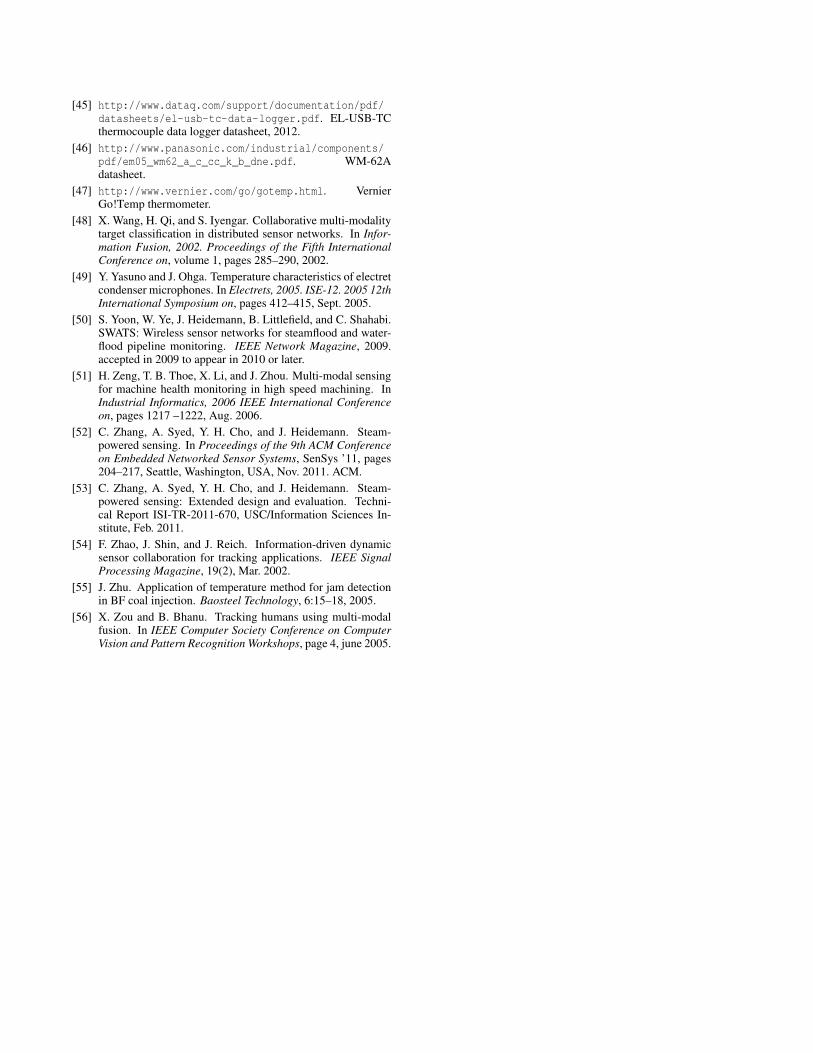
[45] http://www.dataq.com/support/documentation/pdf/

datasheets/el-usb-tc-data-logger.pdf. EL-USB-TCthermocouple data logger datasheet, 2012.

[46] http://www.panasonic.com/industrial/components/

pdf/em05_wm62_a_c_cc_k_b_dne.pdf. WM-62Adatasheet.

[47] http://www.vernier.com/go/gotemp.html. VernierGo!Temp thermometer.

[48] X. Wang, H. Qi, and S. Iyengar. Collaborative multi-modalitytarget classification in distributed sensor networks. In Infor-mation Fusion, 2002. Proceedings of the Fifth InternationalConference on, volume 1, pages 285–290, 2002.

[49] Y. Yasuno and J. Ohga. Temperature characteristics of electretcondenser microphones. In Electrets, 2005. ISE-12. 2005 12thInternational Symposium on, pages 412–415, Sept. 2005.

[50] S. Yoon, W. Ye, J. Heidemann, B. Littlefield, and C. Shahabi.SWATS: Wireless sensor networks for steamflood and water-flood pipeline monitoring. IEEE Network Magazine, 2009.accepted in 2009 to appear in 2010 or later.

[51] H. Zeng, T. B. Thoe, X. Li, and J. Zhou. Multi-modal sensingfor machine health monitoring in high speed machining. InIndustrial Informatics, 2006 IEEE International Conferenceon, pages 1217 –1222, Aug. 2006.

[52] C. Zhang, A. Syed, Y. H. Cho, and J. Heidemann. Steam-powered sensing. In Proceedings of the 9th ACM Conferenceon Embedded Networked Sensor Systems, SenSys ’11, pages204–217, Seattle, Washington, USA, Nov. 2011. ACM.

[53] C. Zhang, A. Syed, Y. H. Cho, and J. Heidemann. Steam-powered sensing: Extended design and evaluation. Techni-cal Report ISI-TR-2011-670, USC/Information Sciences In-stitute, Feb. 2011.

[54] F. Zhao, J. Shin, and J. Reich. Information-driven dynamicsensor collaboration for tracking applications. IEEE SignalProcessing Magazine, 19(2), Mar. 2002.

[55] J. Zhu. Application of temperature method for jam detectionin BF coal injection. Baosteel Technology, 6:15–18, 2005.

[56] X. Zou and B. Bhanu. Tracking humans using multi-modalfusion. In IEEE Computer Society Conference on ComputerVision and Pattern Recognition Workshops, page 4, june 2005.

http://www.dataq.com/support/documentation/pdf/datasheets/el-usb-tc-data-logger.pdf

http://www.dataq.com/support/documentation/pdf/datasheets/el-usb-tc-data-logger.pdf

http://www.panasonic.com/industrial/components/pdf/em05_wm62_a_c_cc_k_b_dne.pdf

http://www.panasonic.com/industrial/components/pdf/em05_wm62_a_c_cc_k_b_dne.pdf

http://www.vernier.com/go/gotemp.html

Documents

Reducing False Alarms with Multi-modal Sensing for ...johnh/PAPERS/Zhang13b.pdf · Reducing False Alarms with Multi-modal Sensing for Pipeline Blockage (Extended) ... machine wear-out