1

Red Wolf (Canis rufus) Population Viability Analysis –

FINAL REPORT FOR U.S. FISH AND WILDLIFE SERVICE (USFWS)

FEASIBILITY STUDY

10 June 2016

Developed by the Red Wolf PVA Team:

Lisa Faust, Ph.D., Lincoln Park Zoo

Joseph Simonis, Ph.D., DAPPER and Lincoln Park Zoo

Rebecca Harrison, Ph.D., USFWS

William Waddell, Point Defiance Zoo and Aquarium

Sarah Long, M.S., Lincoln Park Zoo

Additional modeling feedback/report review provided by:

Kathy Traylor-Holzer, Ph.D., IUCN SSC Conservation Breeding Specialist Group

Pete Benjamin, USFWS

Report Citation:

Faust, L.J., Simonis, J.S., Harrison, R., Waddell, W., Long, S. 2016. Red Wolf (Canis rufus) Population Viability Analysis – Report to U.S. Fish and Wildlife Service. Lincoln Park Zoo, Chicago.

2

Table of Contents

Executive Summary ....................................................................................................................................... 3

Background ................................................................................................................................................... 4

Modeling Approach ...................................................................................................................................... 5

Model Scenarios ............................................................................................................................................ 9

Model Validation ......................................................................................................................................... 12

Model Results Summary ............................................................................................................................. 13

Population History and Current Status ................................................................................................... 13

PVA Results – Baseline (Scenario A) ........................................................................................................ 15

PVA Results – Scenarios With Changes to NENC Parameters ................................................................. 18

PVA Results – Scenarios With Changes to SSP Parameters .................................................................... 20

PVA Results – SSP Population Absorbing NENC Wolves After NENC Termination ................................. 20

PVA Results – Release Scenarios (Connecting SSP and NENC Populations) ........................................... 21

PVA Results – Recovery on Federal Lands Only ...................................................................................... 27

PVA Conclusions .......................................................................................................................................... 28

Appendix 1: Vortex Model Setup Documentation & Supporting Analyses ................................................ 32

Appendix 2. Model Scenario Results Table ................................................................................................. 52

Appendix 3. Literature Cited ....................................................................................................................... 56

Appendix 4. Additional Model Scenarios .................................................................................................... 59

3

Executive Summary BACKGROUND

A Population Viability Analysis (PVA) is a quantitative computer model that can be used to project a population’s long-term demographic and genetic future. In 2013, USFWS and the Red Wolf Species Survival Plan® (SSP) captive breeding program approached experts at the Lincoln Park Zoo to create the Red Wolf PVA team. The goal of this collaboration is to model the viability of the zoo-managed (SSP) and wild, northeastern North Carolina (NENC) red wolf populations, to better understand the conditions under which each population can best persist into the future and how movement of individuals between the populations impacts viability in both. This report summarizes modeling results from a stochastic individual-based model built in Vortex 10.1 for use in USFWS’ Feasibility Review.

POPULATION HISTORY/CURRENT STATUS

A captive red wolf population has been managed in zoos and partner facilities since 1969, growing to 207 wolves at 44 institutions as of 1 January 2015 (our model starting point). Both the captive and wild populations are founded from only 14 wild-caught individuals from a single site in western Louisiana/eastern Texas; currently 12 founder lines are represented. The SSP has retained 89.2% of its founding gene diversity (GD) and the mean inbreeding value (F) is 0.076 (above that of first-cousin matings, 0.0625). The SSP population is space-limited, with current institutions potentially holding 225 wolves.

In 1987, the Recovery Program initiated the first red wolf restoration effort in northeastern North Carolina (NENC), ultimately releasing 165 wolves into NENC and an unsuccessful second reintroduction site. The NENC population had 74 individuals as of 1 January 2015. In the past this population has been as large as 148 individuals, but it has declined from that size over the past decade (Fig. 1a). Since the initiation of this modeling effort, the NENC population has continued to experience a decline, with current population size estimated at 45-60 (USFWS, 2016). Analysis of historical data indicate that mortality in breeding season has been increasing (Fig. A9, Hinton et al. 2015, Hinton et al. in review, Bohling and Waits 2015), disrupting reproductive pairs and lowering reproductive success, and that anthropogenic-caused mortality is the leading cause of death (Hinton et al. 2015). The NENC population has retained 85.4% of its founding GD and its mean F is 0.129 (above that of half-sibling matings, 0.125).

PVA RESULTS Current conditions, without releases from the SSP or improvements to NENC vital rates, will result in extinction of the only remaining wild population of red wolves, typically within 37 years but in some iterations as soon as 8 years. Extinction will likely occur earlier than this timeframe because the population has already declined to lower than the model starting point. However, the NENC population can avoid extinction and be viable, but requires assistance to do so. There were several scenarios that would result in low (<10%) probability of extinction in the next 125 years for the NENC population; the most realistic of these involve a combination of reductions in NENC mortality rates, increases in NENC breeding rates (hypothesized to be achievable by reducing the disruptive effects of breeding-season mortality), and receiving releases from the SSP for a short, intense period (15 years) followed by intermittent releases to maintain genetic health after that. While the SSP population has been maintained at a relatively large population size of more than 150 animals for over 20 years, it needs to increase breeding and increase its population size/space to ensure long-term viability and its ability to serve as a strong source for animals to release to the wild. Model

4

scenarios with growth to 330 or 400 spaces illustrate that the population could benefit substantially in its population genetics and ability to sustain releases from such a change. Currently, space limits population size and, because there are not enough spaces to place pups, fewer breeding recommendations are issued. This management results in the use of contraceptives, separating of pairs during the breeding season, and/or delayed or less frequent breeding opportunities for females. Evidence from other carnivore species suggests that all of these management actions can negatively impact female fertility and reproductive health (Penfold et al. 2014, Asa et al. 2014). To increase from 225 to a population size of 330 or 400 wolves, new resources would need to be identified. The 1990 Recovery Plan stated a goal of retaining 80% GD in 150 years (125 years from the 2015 starting point of the model). Under our various modeling scenarios, when considering the populations separately, 13 of the SSP scenarios had a high (>80%) chance of meeting this benchmark, but only two of the NENC scenarios could do so. However, when considered at the species level with the entire metapopulation, there were 22 model scenarios that had a high chance of retaining 80% GD, illustrating that achieving that recovery plan goal is possible with careful management. These modeling scenarios highlight that red wolves will be a conservation-reliant species, requiring population management: all red wolves will need to be treated as a metapopulation, with occasional movement between the SSP and NENC, and perhaps other populations if they are established, to manage declining gene diversity given its small founding population (Goble et al. 2012). Both populations are small and will face rising inbreeding levels, and our model scenarios include the inbreeding effects that have already been detected (Appendix 1), but careful genetic management and continued, occasional releases to the NENC would help mitigate these effects. With NENC demographic changes and releases, maintaining a functioning wild NENC population is possible. This is a key example of a species that can be best preserved by the “One Plan” approach, where all populations, captive and wild, are considered under an integrated plan for species conservation (Byers et al. 2013).

Background A Population Viability Analysis (PVA) is a quantitative computer model that can be used to project a population’s long-term demographic and genetic future (Beissinger and McCullough, 2002; Morris and Doak, 2002). Models can be used to identify key natural and anthropogenic factors impacting population dynamics. PVAs are typically used to compare a baseline scenario, reflecting the population’s likely future trajectory if current conditions continue, to alternate scenarios which can explore the impact of potential management changes, shifting environmental drivers, or whether uncertainty in parameter values has an impact on model results. These comparisons can help evaluate the relative costs and benefits of possible management actions. Because the future can be uncertain and difficult to predict, model results are most appropriately used to compare between scenarios (e.g. relative to each other) rather than as absolute predictions of what will happen. A PVA is an especially appropriate tool when robust data exist for model parameterization – both on the species biology and on the threats affecting the species’ current and future status. For red wolves, decades of individual-based monitoring has resulted in high quality, long-term datasets that make it possible to base the model on actual historical biological data. This is rare, especially when conducting PVAs for endangered and threatened species. In this sense, the results in this PVA should be especially appropriate for addressing the questions of the USFWS Feasibility review.

5

Red wolves declined in the wild over the 1960s due to habitat loss and predator control programs. The species was listed as endangered in 1967, an ex situ population was established in 1969, and red wolves were considered biologically extinct in the wild in 1980. The first litters of captive pups were born in 1977. In 1987, the Recovery Program initiated the first red wolf restoration effort in northeastern North Carolina (NENC) and began releasing animals from the ex situ population; there was also an unsuccessful second reintroduction site at Great Smoky Mountains National Park in the 1990s. Since reintroductions began in 1987, 165 wolves have been released from the ex situ population (Simonis et al. 2015). Both the captive and wild populations are founded from only 14 wild-caught individuals from western Louisiana/eastern Texas. Currently, the captive and wild populations contain 12 founder lines, with one additional potential founder lineage available via a genome bank if artificial insemination techniques are perfected. The wild population that served as a source for these 14 individuals also went through a severe bottleneck before the capture of these founding wolves.

A Population Habitat and Viability Assessment (PHVA) was previously completed for red wolves (Kelly et al. 1999). Much of the PHVA was not based on detailed analysis of red wolf data from the wild, but rather on a combination of expert opinion and data from other wolves and large canids. The authors recognized the shortcomings of this approach and called for additional modeling (Kelly et al. 1999). The PHVA projected that the NENC population would increase by 20% annually until 2010; the population did follow this trajectory until ~2005, when it began to decline, with the pace of decline increasing rapidly since 2010.

In 2013, USFWS and the Red Wolf Species Survival Plan® (SSP) captive breeding program approached experts at the Lincoln Park Zoo to create the Red Wolf PVA team. The goal of this collaboration is to model the viability of the zoo-managed (SSP) and wild, northeastern North Carolina (NENC) red wolf populations, to better understand the conditions under which each population can best persist into the future and how movement of individuals between the populations impacts viability in both. The team developed an SSP-only model using ZooRisk software (Earnhardt et al. 2008), and published a final report on the PVA to the zoo community (Simonis et al. 2015a). This report reflects an updated metapopulation modeling approach using Vortex software, which has additional features that make it suited for modeling spatially separated populations that are connected via movement of individuals between the populations. The model and this report has been peer-reviewed by the IUCN SSC Conservation Breeding Specialist Group (CBSG). In 2016-2017, anticipated products include one or more manuscripts on the PVA. The information in this PVA and subsequent products can feed into future Recovery Planning documents including Species Assessments, 5-year Status Reviews, Consultations, Rule Revisions, and Recovery Plan revisions.

Modeling Approach We developed a stochastic, individual-based population model in Vortex 10.1.4.0 software, a widely used PVA modeling software package (Lacy and Pollack 2015). For more detailed descriptions of Vortex and how it is applied in PVAs, see Lacy (1993, 2000) and Lacy et al. (2015). The red wolf model has two subpopulations: SSP and NENC. The model is individual-based, meaning it tracks every animal (current and future) in the population over time. After being initiated with the starting population, the model steps through an annual event cycle (e.g., births, transfers between subpopulations, deaths, aging, censusing) for all individuals.

For both the NENC and SSP populations, animals are individually identified and tracked in a studbook, an electronic database maintained using PopLink 2.4 (Faust et al. 2012). The red wolf studbook contains

6

both populations’ demographic and genetic history including births, deaths, transfers between zoos or between the SSP and NENC population, and pedigree relationships tracing back to the original founders (Waddell 2015). Additional NENC data are taken from USFWS databases. We parameterized the Vortex model with data from these datasets.

GENERAL MODEL SETUP

Full details on model parameterization and data analyses are presented in Appendix 1. This is a brief overview of the setup for the baseline model scenario (parameters are bolded and parameter values used in the model are underlined; EV = if a parameter includes environmental variation):

Model Timeframe: 125 years Model results are reported at 150 years from the 1990 Recovery Plan (i.e. 2140, or 125 years from 2015).

Initial Population: SSP = 201 wolves; NENC = 74 wolves The model was initialized with a starting population of the living animals in each population as of 1 January 2015, extracted from the studbook. The model tracks these individual’s age, sex, subpopulation (SSP or NENC), and genetic relatedness to other individuals over time. In addition, the starting individuals were paired with their existing mate if they were currently paired. As of 1 January 2015, the SSP had 201 individuals (87 males, 114 females) and the NENC population had 74 individuals (34 males, 40 females). For age distributions see Appendix 1, Fig. A5.

Movement between populations: baseline scenario = off The baseline scenario models the SSP and NENC as isolated populations, since as of 2015 USFWS had ceased releases into the NENC. In alternate scenarios, the model randomly selects animals (within specified age classes based on a specified number of releases) from the SSP population to move into the NENC population. Equal numbers of males and females are moved. Releases can only occur in years where the SSP’s population size is larger than 80% of Carrying Capacity (see below). The model is behaviorally naive in that it assumes that as soon as an individual is released to the wild, it behaves like a wild wolf with NENC demographic rates. Note that although in the past some wolves were “removed” from the wild and transferred into the SSP or euthanized based on requests for removals from the NENC population due to human-wildlife conflict, in this modeling exercise we are not including these types of removals from the NENC population.

Inbreeding Depression: Includes observed impacts on litter size, sex ratio and pup mortality for SSP and NENC In a small population with a limited founder base, mating between close relatives (inbreeding) is often unavoidable and can have potential negative impacts on population demographics and viability. Inbreeding effects were previously documented for the SSP population (Rabon and Waddell 2010), but were not detected for the NENC population (Brzeski et al. 2014). As part of this modeling effort, we re-analyzed SSP and NENC data for effects of inbreeding depression, and found statistically significant effects on offspring sex ratio, litter size, and pup mortality for both populations. We included these effects in the model (see parameter descriptions below and Appendix 1).

Catastrophes: 2.9% chance per year of a 50% reduction in survival for NENC population Catastrophes are rare events that occur stochastically: in any given model year, Vortex assesses whether it is a catastrophe year or not and alters vital rates for that single year accordingly. Potential catastrophes that might threaten the NENC population include disease outbreaks, hurricanes, and fires. Our selected value for catastrophes was based on the frequency and severity of catastrophes observed in a review of 88 wild vertebrate species (Reed et al. 2003), which found a

7

frequency of 14% per generation (red wolf generation length = 4.9 years based on wild data, See Appendix 1). It is assumed that the SSP is buffered from catastrophes, as it is spread across multiple institutions and adverse events can be mitigated by human management.

Reproductive system: long-term monogamy Red wolves form long-term bonded pairs; in the NENC pairs typically remain together until a mate dies and then the surviving wolf may re-pair, while in the SSP pairs are typically kept together unless the mate becomes post-reproductive, the mate dies, the pair is behaviorally incompatible, or genetic relationships become mismatched. In the model the reproductive system was set at long-term monogamy.

Carrying capacity (K): SSP = 225, NENC = 150 This variable is used to limit population growth in the model; when the population is larger than K at the end of the year, Vortex probabilistically culls across all age and sex classes to bring the population back approximately to K.

In the NENC, K = 150 based on a previous estimate by USFWS (Kelly et al. 1999) of the potential number of individuals that could be held at the original reintroduction site of Alligator River National Wildlife Refuge if the population had access to the whole landscape of the 5-county NEP area. In the past the maximum estimated population size was 148 individuals, and when at that size there was not strong observed intraspecific competition or density-dependent effects, so the population was likely not truly at ecological K (Gese et al. 2015; Hinton et al. in review). However, for the model 150 was chosen as a cap that the population would likely not be able to exceed.

In the SSP, K = 225 based on the population size that can be held in the current space available in zoos (Simonis et al. 2015a). This size/space is not necessarily equivalent to the number of exhibits or enclosures: because of the social structure of wolves, two or more animals are frequently housed together depending on enclosure size, location, and intent (exhibit or off-site). In the model, K reflects the number of individuals, but not the explicit number of spaces/exhibits. In the model the SSP population is “bred to maintain the population at K”, meaning that each year the model assesses the current size against K, takes into consideration the estimated number of deaths expected in the year, average breeding success of recommended breeding pairs, litter size, and pup survival, and determines the number of breeding pairs to make (similar to the SSP breeding recommendation process for the year).

Proportion of females in the breeding pool: SSP = 93%; NENC = 52.5%, EV = 7.9% Each year, the model stochastically pulls a fraction of reproductive-aged (ages 2-10) females into the potential breeding pool (for both unpaired and paired females). This % of adult females breeding was 93% for the SSP based on the % of non-breeders in the current SSP who are unable to breed for health or reproductive reasons (6/87 individuals, or 7%; Waddell and Long 2014). The NENC rate = 52.5%, EV (Standard Deviation) = 7.9% based on the average observed number of females in wolf-wolf pairs from 2000-2014 (Appendix 1, Table A2).

Proportion of males in the breeding pool: SSP = 94%; NENC = 88% Un-paired, reproductive-aged (ages 2-12) males are pulled into the breeding pool based on the % of males in breeding pool. The SSP rate = 94% based on the % of non-breeders in the current SSP who are unable to breed for health or reproductive reasons (4/68 individuals, or 6%; Waddell and Long 2014). The NENC rate = 88% based on excluding the average percentage of males in wolf-non-wolf pairs from 2000-2014, 12% (Appendix 1, Table A2).

Criteria for separating long-term pair: SSP only = 25% In the SSP population, pairs had a 25% probability of being split in any given year and going back into the respective breeding pools. This frequency was based on assessments from the last 15 years of SSP breeding recommendations from SSP Breeding and Transfer Plans. All pairs have an equal chance of being split each year, not based on genetic value or past reproductive performance.

8

Genetic Management: SSP = on; NENC = off For both the SSP and NENC populations, the model is initialized with the existing breeding pairs

as of January 2015 (for the SSP, this was 37 pairs; for the NENC, it was six pairs). For the SSP, genetic management is turned on to simulate the SSP process of managing by mean kinship (MK), the genetic relatedness of an individual to the rest of the population. In any given year, females in the breeding pool that do not have a mate are paired with the next available male with the lowest MK value (i.e. individuals from more rare genetic lines get paired first). To avoid creating excessively inbred litters, if the kinship between the female and a potential male exceeds 1 – 90% * GD (current population gene diversity), the next male on the list is selected (re-trying a maximum of 10 times). This process uses a static MK list, (i.e., one that is only sorted at the beginning of the model year) rather than resorted after each pair has offspring. In the NENC, genetic management = off; in the model unpaired animals from the breeding pools are randomly paired because wild wolves choose their own mates except under coyote management regimes, which is simulated in other model parameters (i.e. proportion of females in the breeding pool).

Female breeding success: SSP = 19%; NENC = 60% For any females in the breeding pool that are paired through the pairing process (randomly in

the NENC or via genetic management for the SSP), the model stochastically assesses whether the female successfully breeds based on the distribution of litters (which Vortex calls broods) per year (i.e. the percentage of unsuccessful (“0 litters”) or successful (“1 litter”) per year). For the SSP, 81% of paired females have 0 litters, and 19% have 1 litter based on the proportion of SSP breeding recommendations that result in a litter before the next breeding and transfer plan is issued (2001-2013 data; Appendix 1, Table A1). For the NENC, 40% have 0 litters, 60% have 1 litter based on the average annual % of wolf-wolf pairs that produced a litter (2000-2014 data; Appendix 1, Table A2).

Reproductive success of these pairs is modeled as random and not based on age, genetic value, or reproductive history (i.e. the model does not take into consideration whether the individual is a “proven breeder”, a young or old reproductive-aged animal, or a genetically valuable individual); this may be an optimistic assumption. For several canid and felid SSP populations, breeding success of recommended pairs is based on several factors, including female age and past reproductive history (Saunders et al. 2014; K. Traylor-Holzer, pers. comm.); however, for red wolves these factors have not been investigated.

Litter Size: Range 1-10; litter size higher in NENC; as inbreeding coefficient increases, litter size decreases; Females can only have one litter per year, at most. If a female is stochastically selected to have a litter, the number of offspring per litter distribution is used to determine the size of her litter. Each litter is between 1 and 10 (based on studbook data), with the number of offspring varying based on statistically significant patterns in the historical data for both populations, where litter size is significantly higher in the NENC population, and as inbreeding coefficient increases in both populations litter size significantly decreases; see Appendix 1 and Fig. A2, A10 for more details.

Offspring sex ratio: as inbreeding coefficient increases, higher probability of male offspring Offspring sex ratio is assigned stochastically, and does not differ between SSP and NENC populations. Sex ratio varies with inbreeding coefficient based on statistically significant patterns in the historical data for both subpopulations: as inbreeding coefficient increases there is a higher probability of a male-biased offspring sex ratio; see Appendix 1 and Fig. A1 for more explanation.

9

Model Scenarios Our modeling was focused on evaluating the population’s viability overall as well as the progress towards meeting the recovery goals laid out in the 1990 Recovery Plan:

1. Develop an ex situ population of at least 330 animals managed at 30 or more breeding facilities and zoos.

2. Establish and maintain at least three in situ red wolf populations totaling at least 220 animals. 3. Preserve at least 80% of the population’s founding genetic diversity for 150 years (i.e., until the

year 2140). Specifically, we were interested in:

1. Under current demographic rates and management (i.e. no releases), are the SSP and NENC populations viable for 125 years?

2. What changes to vital rates would create a viable NENC population? 3. If coyote impacts changed (increased or decreased), how would it impact the NENC population?

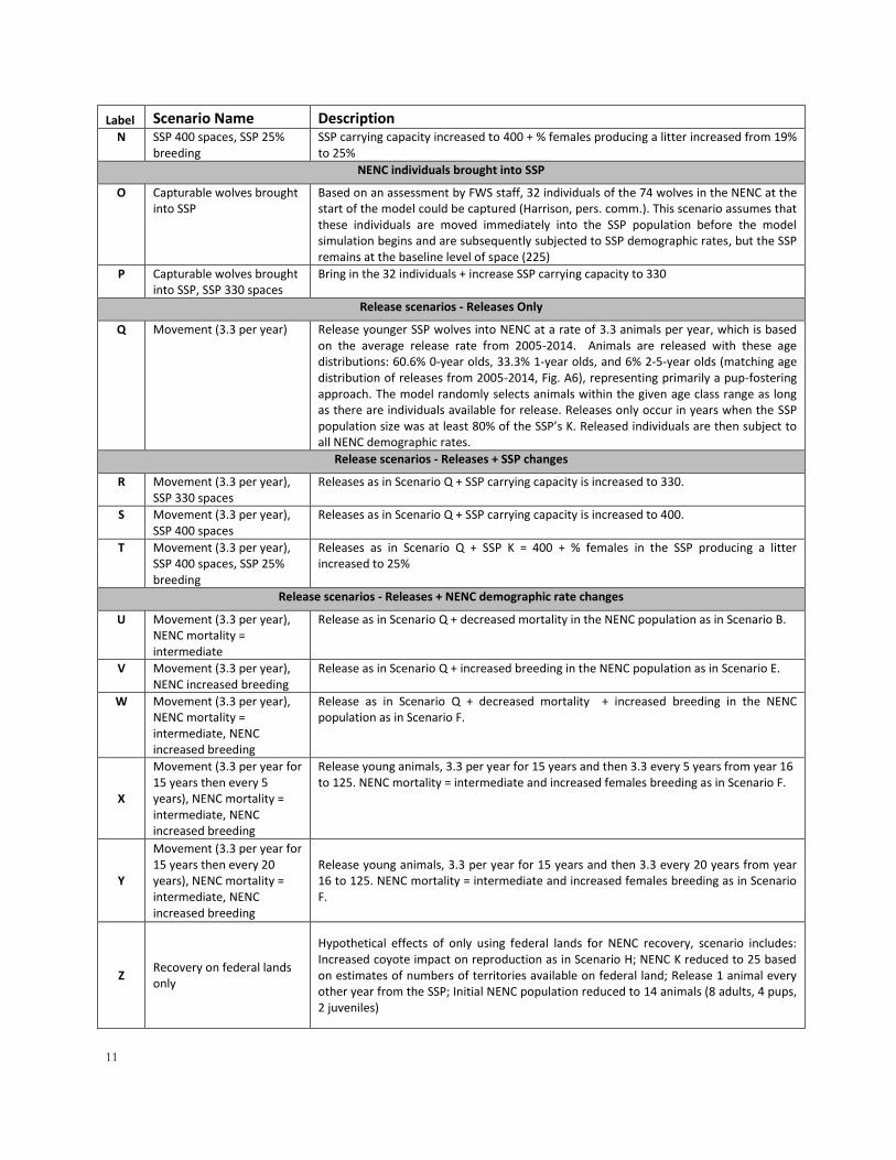
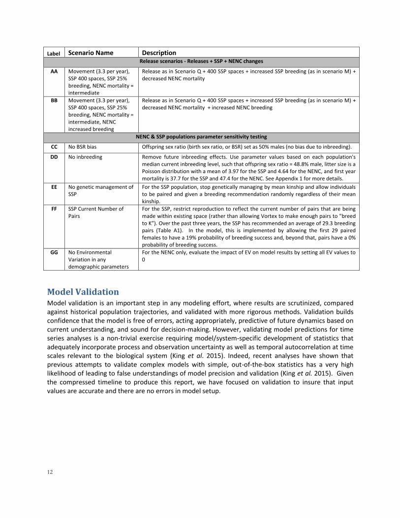
Table 1 details the model scenarios explored in comparison to the baseline model described above, with alterations in parameter setup noted in the “Description” column; see Appendix 1 for additional details.

Additional model scenarios that were run for the preliminary report but are less essential to highlight the main modeling results are included in Appendix 4.

Table 1. Red wolf PVA model scenarios

Label Scenario Name Description A Baseline SSP and NENC populations uncoupled (separate, no releases) with baseline demographic

rates as described above

NENC population - demographic rate changes (survival, reproduction)

B NENC mortality = intermediate

NENC mortality rates are decreased to “intermediate” levels, calculated as the midpoint value between the SSP and NENC rates, for age classes 1-16 (Table A3). Anthropogenic mortality is the leading cause of death for red wolves (Hinton et al. 2015). Evidence suggests that anthropogenic mortality in the population is additive rather than compensatory (Sparkman et al. 2011), suggesting that if human-caused mortalities were reduced, the overall mortality rates for the population would be lower. USFWS managers also suggest that in the population’s early history there were management and health-related issues which, with experience, are now better managed; this is supported by the decreasing trend in per capita mortality over time (Appendix 1, Fig. A8). Although the mortality values used in this scenario are hypothetical, they generally represent a scenario in which anthropogenic (and other) mortality sources are reduced but not reduced to levels as low as the captive SSP population.

C NENC mortality = SSP mortality

NENC mortality rates are decreased to SSP mortality rates for age classes 1-16 (Table A3).

D NENC mortality = Intermediate, no inbreeding depression

NENC has intermediate mortality rates + elimination of inbreeding depression's impact on offspring sex ratio, infant mortality, and litter size as described in scenario DD.

10

Label Scenario Name Description E Increased females breeding

NENC % NENC females breeding increased to 70% based on the highest breeding rates observed in the past, when in 2003-4 the population had 71.4% of females in wolf-wolf pairs (Table A2). We hypothesize that these rates can be achieved again by shifting mortality. Over the history of the population, the timing of mortality in the year has shifted such that in more recent years, mortality (primarily anthropogenic) has occurred fall through winter (i.e. in the fall hunting season), which corresponds to red wolf pre-breeding and breeding season (See Fig. A9; Hinton et al. 2015, Hinton et al. in review, Bohling and Waits 2015). When mortality occurs during this time of year, wolves do not have time to form a new pair bond naturally or via USFWS management actions, disrupting reproduction for the season. If late season, anthropogenic mortality is reduced allowing wolves more time to repair if a mate is killed, higher breeding rates should be achievable (Hinton et al. 2015). While shifts in the timing of mortality would support the increased breeding rate modeled here, the actual mortality rates in this scenario remain unchanged.

F NENC mortality = intermediate, Increased females breeding NENC

NENC has intermediate mortality rates + increased % females breeding. This scenario represents ideal management of demographic rates, where anthropogenic mortality is reduced to the point that overall mortality is reduced, and observed mortality is less concentrated in the pre-breeding and breeding seasons, resulting in higher % females breeding.

G Reduced coyote impact % NENC males in the breeding pool was increased to 100%, assuming no males are mated with coyote females. % NENC females in breeding pool was increased to 68.8%, based on the average annual rate of wolf-canid pairs (i.e. pairs with either a wolf or coyote are replaced by pairs with only wolves) that have been observed 2000-2014 (Table A4). If all wolves were able to make wolf-wolf pairs, reproduction would increase. We hypothesize that these effects might take place if the wolf population was large enough that wolves outcompeted coyotes for breeding partners or territories, and/or if the coyote population was managed through a placeholder approach (Gese et al. 2015, Gese and Terletzky 2015, Bohling et al. 2016).

H Increased coyote impact Assumes that if the coyote population increases or if coyotes are less managed to avoid impacts on the wolf population, then wolf breeding would be further negatively impacted as coyotes would more frequently pair with wolves. To simulate this, we took the average rate of male and female wolves in wolf-coyote breeding pairs (12% and 16.3%, respectfully) and doubled those rates (to 24% and 32.6%); this reduces the % NENC males entering the (wolf) breeding pool from 88% to 76% and females entering the breeding pool from 52.5% to 36.2%. This reduces the breeding pool (of wolf-wolf pairs), which limits the genetic population dynamics as well (fewer pairs have offspring).

I NENC mortality = intermediate, reduced coyote impact

NENC population has intermediate mortality rates + increased breeding rates as in Scenario G.

J NENC mortality = intermediate, Increased coyote impact

NENC population has intermediate mortality rates + decreased breeding rates decreased as in Scenario H.

SSP - increased space and breeding

K SSP 330 spaces SSP carrying capacity increased to 330 based on the target set in the 1990 Recovery Plan (USFWS 1990).

L SSP 400 spaces SSP carrying capacity increased to 400 based on previous modeling work (Simonis et al. 2015b)

M SSP 330 spaces, SSP 25% breeding

SSP carrying capacity increased to 330 + % females producing a litter increased from 19% to 25%. Although the percentage of paired females that successfully breed with their recommended mate in the SSP has achieved a maximum of 34.6% (Table A1), population managers consider this to be overly optimistic for a sustained period of time (Waddell, personal communication). In discussions with population managers, the PVA team decided that 25% was a reasonable, if challenging, value to achieve on an annual basis (Waddell, personal communication).

11

Label Scenario Name Description N SSP 400 spaces, SSP 25%

breeding SSP carrying capacity increased to 400 + % females producing a litter increased from 19% to 25%

NENC individuals brought into SSP

O Capturable wolves brought into SSP

Based on an assessment by FWS staff, 32 individuals of the 74 wolves in the NENC at the start of the model could be captured (Harrison, pers. comm.). This scenario assumes that these individuals are moved immediately into the SSP population before the model simulation begins and are subsequently subjected to SSP demographic rates, but the SSP remains at the baseline level of space (225)

P Capturable wolves brought into SSP, SSP 330 spaces

Bring in the 32 individuals + increase SSP carrying capacity to 330

Release scenarios - Releases Only

Q Movement (3.3 per year) Release younger SSP wolves into NENC at a rate of 3.3 animals per year, which is based on the average release rate from 2005-2014. Animals are released with these age distributions: 60.6% 0-year olds, 33.3% 1-year olds, and 6% 2-5-year olds (matching age distribution of releases from 2005-2014, Fig. A6), representing primarily a pup-fostering approach. The model randomly selects animals within the given age class range as long as there are individuals available for release. Releases only occur in years when the SSP population size was at least 80% of the SSP’s K. Released individuals are then subject to all NENC demographic rates.

Release scenarios - Releases + SSP changes

R Movement (3.3 per year), SSP 330 spaces

Releases as in Scenario Q + SSP carrying capacity is increased to 330.

S Movement (3.3 per year), SSP 400 spaces

Releases as in Scenario Q + SSP carrying capacity is increased to 400.

T Movement (3.3 per year), SSP 400 spaces, SSP 25% breeding

Releases as in Scenario Q + SSP K = 400 + % females in the SSP producing a litter increased to 25%

Release scenarios - Releases + NENC demographic rate changes

U Movement (3.3 per year), NENC mortality = intermediate

Release as in Scenario Q + decreased mortality in the NENC population as in Scenario B.

V Movement (3.3 per year), NENC increased breeding

Release as in Scenario Q + increased breeding in the NENC population as in Scenario E.

W Movement (3.3 per year), NENC mortality = intermediate, NENC increased breeding

Release as in Scenario Q + decreased mortality + increased breeding in the NENC population as in Scenario F.

X

Movement (3.3 per year for 15 years then every 5 years), NENC mortality = intermediate, NENC increased breeding

Release young animals, 3.3 per year for 15 years and then 3.3 every 5 years from year 16 to 125. NENC mortality = intermediate and increased females breeding as in Scenario F.

Y

Movement (3.3 per year for 15 years then every 20 years), NENC mortality = intermediate, NENC increased breeding

Release young animals, 3.3 per year for 15 years and then 3.3 every 20 years from year 16 to 125. NENC mortality = intermediate and increased females breeding as in Scenario F.

Z Recovery on federal lands only

Hypothetical effects of only using federal lands for NENC recovery, scenario includes: Increased coyote impact on reproduction as in Scenario H; NENC K reduced to 25 based on estimates of numbers of territories available on federal land; Release 1 animal every other year from the SSP; Initial NENC population reduced to 14 animals (8 adults, 4 pups, 2 juveniles)

12

Label Scenario Name Description Release scenarios - Releases + SSP + NENC changes

AA Movement (3.3 per year), SSP 400 spaces, SSP 25% breeding, NENC mortality = intermediate

Release as in Scenario Q + 400 SSP spaces + increased SSP breeding (as in scenario M) + decreased NENC mortality

BB Movement (3.3 per year), SSP 400 spaces, SSP 25% breeding, NENC mortality = intermediate, NENC increased breeding

Release as in Scenario Q + 400 SSP spaces + increased SSP breeding (as in scenario M) + decreased NENC mortality + increased NENC breeding

NENC & SSP populations parameter sensitivity testing

CC No BSR bias Offspring sex ratio (birth sex ratio, or BSR) set as 50% males (no bias due to inbreeding).

DD No inbreeding Remove future inbreeding effects. Use parameter values based on each population's median current inbreeding level, such that offspring sex ratio = 48.8% male, litter size is a Poisson distribution with a mean of 3.97 for the SSP and 4.64 for the NENC, and first year mortality is 37.7 for the SSP and 47.4 for the NENC. See Appendix 1 for more details.

EE No genetic management of SSP

For the SSP population, stop genetically managing by mean kinship and allow individuals to be paired and given a breeding recommendation randomly regardless of their mean kinship.

FF SSP Current Number of Pairs

For the SSP, restrict reproduction to reflect the current number of pairs that are being made within existing space (rather than allowing Vortex to make enough pairs to "breed to K”). Over the past three years, the SSP has recommended an average of 29.3 breeding pairs (Table A1). In the model, this is implemented by allowing the first 29 paired females to have a 19% probability of breeding success and, beyond that, pairs have a 0% probability of breeding success.

GG No Environmental Variation in any demographic parameters

For the NENC only, evaluate the impact of EV on model results by setting all EV values to 0

Model Validation Model validation is an important step in any modeling effort, where results are scrutinized, compared against historical population trajectories, and validated with more rigorous methods. Validation builds confidence that the model is free of errors, acting appropriately, predictive of future dynamics based on current understanding, and sound for decision-making. However, validating model predictions for time series analyses is a non-trivial exercise requiring model/system-specific development of statistics that adequately incorporate process and observation uncertainty as well as temporal autocorrelation at time scales relevant to the biological system (King et al. 2015). Indeed, recent analyses have shown that previous attempts to validate complex models with simple, out-of-the-box statistics has a very high likelihood of leading to false understandings of model precision and validation (King et al. 2015). Given the compressed timeline to produce this report, we have focused on validation to insure that input values are accurate and there are no errors in model setup.

13

Model Results Summary Throughout the results, we refer to model scenarios by letter, i.e. (Scenario A) or (A); refer back to Table 1 for full scenario descriptions. We use the following abbreviations for summary statistics:

Abbreviation Description

P(E) Probability of extinction in 125 years (i.e. the # of extinct iterations/total # of iterations)

GD Mean gene diversity retained in 125 years, calculated across surviving (non-extinct) model iterations

F Mean inbreeding coefficient in 125 years, calculated across surviving (non-extinct) model iterations

N Mean population size in 125 years, calculated across all 1000 model iterations (extant and extinct)

TE Median time to extinction for iterations that go extinct (only reported if the population went extinct in at least 50% of simulations)

P(80GD) Probability of population maintaining 80% GD at 125 years, calculated across all surviving (non-extinct) model iterations

Note that GD, F, and N all have variability associated with them due to the stochastic nature of the model dynamics, and this variability conveys the range of possible future outcomes under a model scenario. For GD, F, and N we also present the standard deviation (+ 1 SD) for any mean values reported. See Appendix 2 for a table summarizing all model results across all scenarios for each population.

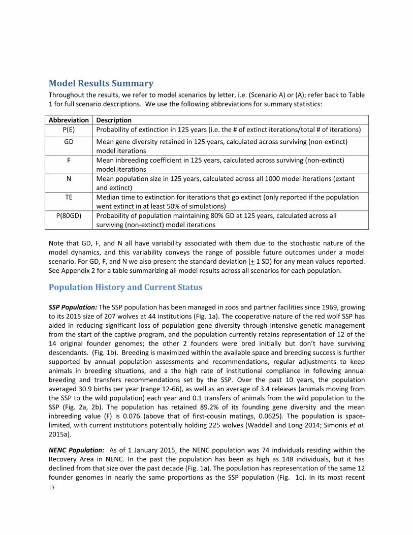
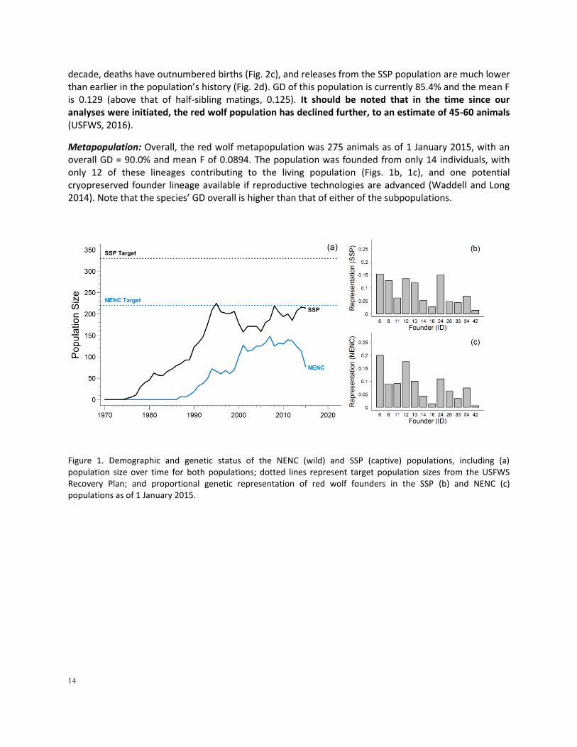
Population History and Current Status SSP Population: The SSP population has been managed in zoos and partner facilities since 1969, growing to its 2015 size of 207 wolves at 44 institutions (Fig. 1a). The cooperative nature of the red wolf SSP has aided in reducing significant loss of population gene diversity through intensive genetic management from the start of the captive program, and the population currently retains representation of 12 of the 14 original founder genomes; the other 2 founders were bred initially but don’t have surviving descendants. (Fig. 1b). Breeding is maximized within the available space and breeding success is further supported by annual population assessments and recommendations, regular adjustments to keep animals in breeding situations, and a the high rate of institutional compliance in following annual breeding and transfers recommendations set by the SSP. Over the past 10 years, the population averaged 30.9 births per year (range 12-66), as well as an average of 3.4 releases (animals moving from the SSP to the wild population) each year and 0.1 transfers of animals from the wild population to the SSP (Fig. 2a, 2b). The population has retained 89.2% of its founding gene diversity and the mean inbreeding value (F) is 0.076 (above that of first-cousin matings, 0.0625). The population is space-limited, with current institutions potentially holding 225 wolves (Waddell and Long 2014; Simonis et al. 2015a).

NENC Population: As of 1 January 2015, the NENC population was 74 individuals residing within the Recovery Area in NENC. In the past the population has been as high as 148 individuals, but it has declined from that size over the past decade (Fig. 1a). The population has representation of the same 12 founder genomes in nearly the same proportions as the SSP population (Fig. 1c). In its most recent

14

decade, deaths have outnumbered births (Fig. 2c), and releases from the SSP population are much lower than earlier in the population’s history (Fig. 2d). GD of this population is currently 85.4% and the mean F is 0.129 (above that of half-sibling matings, 0.125). It should be noted that in the time since our analyses were initiated, the red wolf population has declined further, to an estimate of 45-60 animals (USFWS, 2016).

Metapopulation: Overall, the red wolf metapopulation was 275 animals as of 1 January 2015, with an overall GD = 90.0% and mean F of 0.0894. The population was founded from only 14 individuals, with only 12 of these lineages contributing to the living population (Figs. 1b, 1c), and one potential cryopreserved founder lineage available if reproductive technologies are advanced (Waddell and Long 2014). Note that the species’ GD overall is higher than that of either of the subpopulations.

Figure 1. Demographic and genetic status of the NENC (wild) and SSP (captive) populations, including (a) population size over time for both populations; dotted lines represent target population sizes from the USFWS Recovery Plan; and proportional genetic representation of red wolf founders in the SSP (b) and NENC (c) populations as of 1 January 2015.

15

Figure 2. Annual numbers of demographic events for the SSP (a, b) and NENC (c, d) populations. (a) and (c) show births in green and deaths in red (note that the NENC deaths also include individuals that were lost to follow-up or “LTF”, which are missing, and presumed dead). (b) and (d) show imports in green and exports in red. Imports/exports are in reference to the focal population, thus in (b), imports are animals returning into the SSP from the wild, and exports are releases into the wild; in (d) imports are releases into the wild, and exports are animals transferred into the SSP.

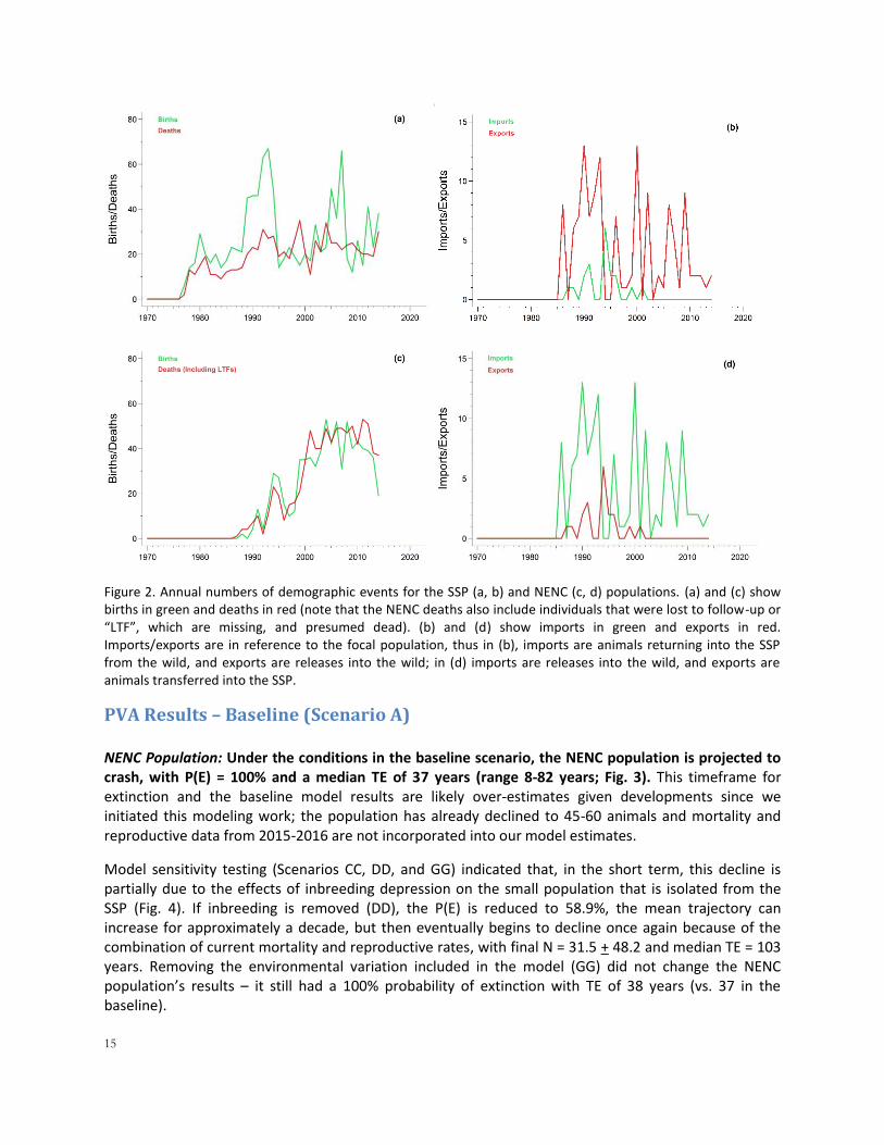
PVA Results – Baseline (Scenario A) NENC Population: Under the conditions in the baseline scenario, the NENC population is projected to crash, with P(E) = 100% and a median TE of 37 years (range 8-82 years; Fig. 3). This timeframe for extinction and the baseline model results are likely over-estimates given developments since we initiated this modeling work; the population has already declined to 45-60 animals and mortality and reproductive data from 2015-2016 are not incorporated into our model estimates.

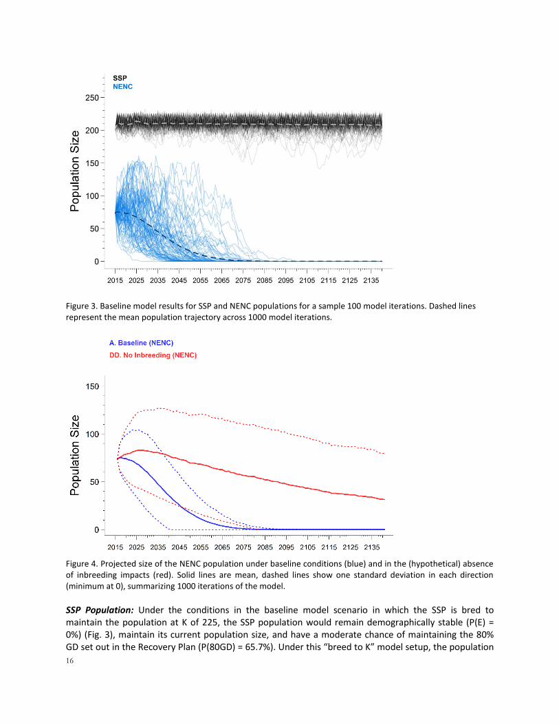
Model sensitivity testing (Scenarios CC, DD, and GG) indicated that, in the short term, this decline is partially due to the effects of inbreeding depression on the small population that is isolated from the SSP (Fig. 4). If inbreeding is removed (DD), the P(E) is reduced to 58.9%, the mean trajectory can increase for approximately a decade, but then eventually begins to decline once again because of the combination of current mortality and reproductive rates, with final N = 31.5 + 48.2 and median TE = 103 years. Removing the environmental variation included in the model (GG) did not change the NENC population’s results – it still had a 100% probability of extinction with TE of 38 years (vs. 37 in the baseline).

16

Figure 3. Baseline model results for SSP and NENC populations for a sample 100 model iterations. Dashed lines represent the mean population trajectory across 1000 model iterations.

Figure 4. Projected size of the NENC population under baseline conditions (blue) and in the (hypothetical) absence of inbreeding impacts (red). Solid lines are mean, dashed lines show one standard deviation in each direction (minimum at 0), summarizing 1000 iterations of the model.

SSP Population: Under the conditions in the baseline model scenario in which the SSP is bred to maintain the population at K of 225, the SSP population would remain demographically stable (P(E) = 0%) (Fig. 3), maintain its current population size, and have a moderate chance of maintaining the 80% GD set out in the Recovery Plan (P(80GD) = 65.7%). Under this “breed to K” model setup, the population

17

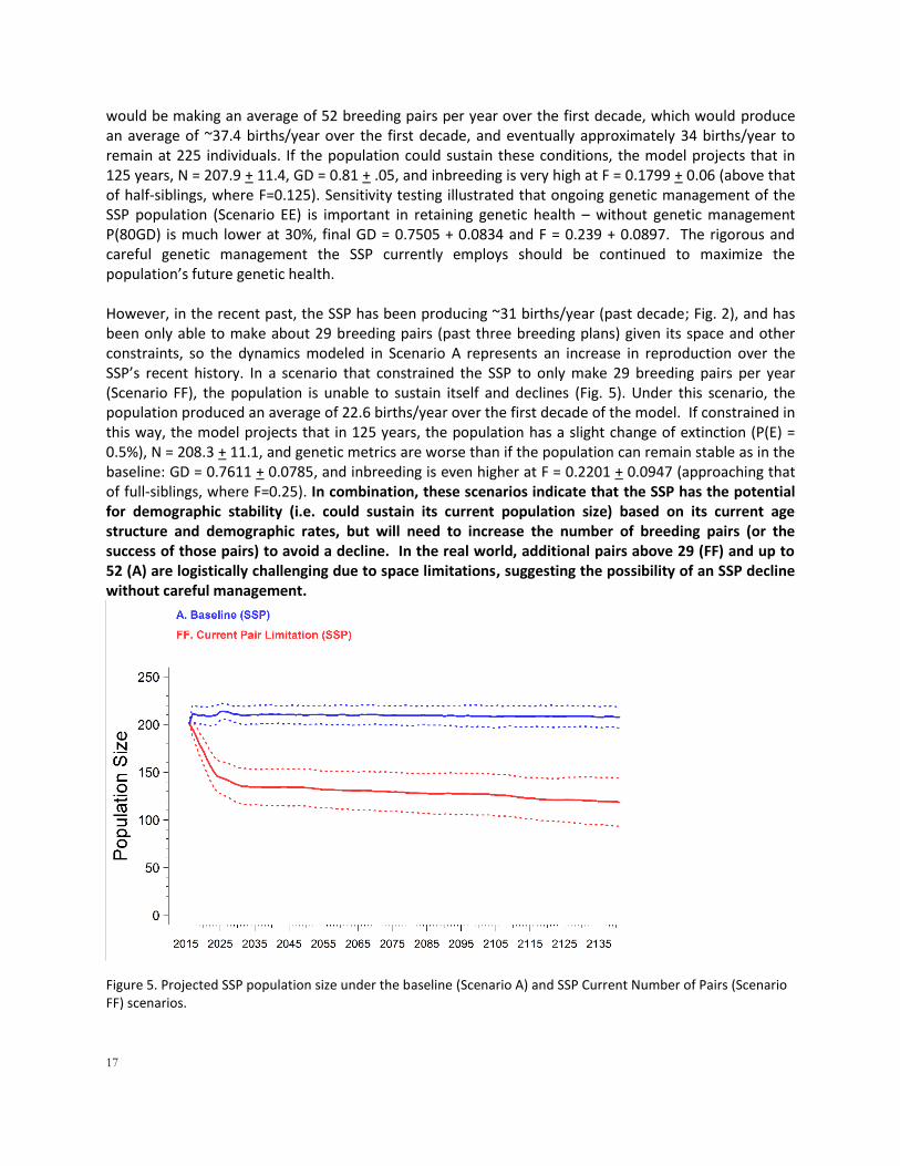
would be making an average of 52 breeding pairs per year over the first decade, which would produce an average of ~37.4 births/year over the first decade, and eventually approximately 34 births/year to remain at 225 individuals. If the population could sustain these conditions, the model projects that in 125 years, N = 207.9 + 11.4, GD = 0.81 + .05, and inbreeding is very high at F = 0.1799 + 0.06 (above that of half-siblings, where F=0.125). Sensitivity testing illustrated that ongoing genetic management of the SSP population (Scenario EE) is important in retaining genetic health – without genetic management P(80GD) is much lower at 30%, final GD = 0.7505 + 0.0834 and F = 0.239 + 0.0897. The rigorous and careful genetic management the SSP currently employs should be continued to maximize the population’s future genetic health. However, in the recent past, the SSP has been producing ~31 births/year (past decade; Fig. 2), and has been only able to make about 29 breeding pairs (past three breeding plans) given its space and other constraints, so the dynamics modeled in Scenario A represents an increase in reproduction over the SSP’s recent history. In a scenario that constrained the SSP to only make 29 breeding pairs per year (Scenario FF), the population is unable to sustain itself and declines (Fig. 5). Under this scenario, the population produced an average of 22.6 births/year over the first decade of the model. If constrained in this way, the model projects that in 125 years, the population has a slight change of extinction (P(E) = 0.5%), N = 208.3 + 11.1, and genetic metrics are worse than if the population can remain stable as in the baseline: GD = 0.7611 + 0.0785, and inbreeding is even higher at F = 0.2201 + 0.0947 (approaching that of full-siblings, where F=0.25). In combination, these scenarios indicate that the SSP has the potential for demographic stability (i.e. could sustain its current population size) based on its current age structure and demographic rates, but will need to increase the number of breeding pairs (or the success of those pairs) to avoid a decline. In the real world, additional pairs above 29 (FF) and up to 52 (A) are logistically challenging due to space limitations, suggesting the possibility of an SSP decline without careful management.

Figure 5. Projected SSP population size under the baseline (Scenario A) and SSP Current Number of Pairs (Scenario FF) scenarios.

18

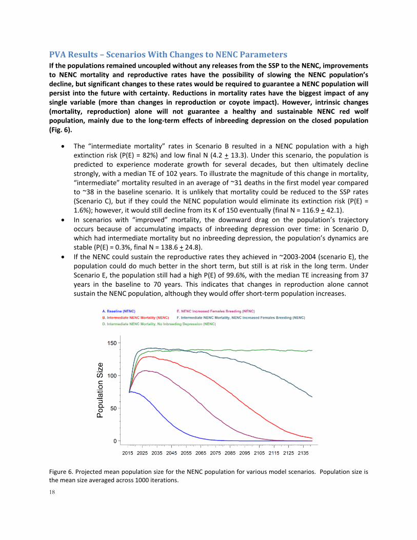
PVA Results – Scenarios With Changes to NENC Parameters If the populations remained uncoupled without any releases from the SSP to the NENC, improvements to NENC mortality and reproductive rates have the possibility of slowing the NENC population’s decline, but significant changes to these rates would be required to guarantee a NENC population will persist into the future with certainty. Reductions in mortality rates have the biggest impact of any single variable (more than changes in reproduction or coyote impact). However, intrinsic changes (mortality, reproduction) alone will not guarantee a healthy and sustainable NENC red wolf population, mainly due to the long-term effects of inbreeding depression on the closed population (Fig. 6).

The “intermediate mortality” rates in Scenario B resulted in a NENC population with a high extinction risk (P(E) = 82%) and low final N (4.2 + 13.3). Under this scenario, the population is predicted to experience moderate growth for several decades, but then ultimately decline strongly, with a median TE of 102 years. To illustrate the magnitude of this change in mortality, “intermediate” mortality resulted in an average of ~31 deaths in the first model year compared to ~38 in the baseline scenario. It is unlikely that mortality could be reduced to the SSP rates (Scenario C), but if they could the NENC population would eliminate its extinction risk (P(E) = 1.6%); however, it would still decline from its K of 150 eventually (final N = 116.9 + 42.1).

In scenarios with “improved” mortality, the downward drag on the population’s trajectory occurs because of accumulating impacts of inbreeding depression over time: in Scenario D, which had intermediate mortality but no inbreeding depression, the population’s dynamics are stable (P(E) = 0.3%, final N = 138.6 + 24.8).

If the NENC could sustain the reproductive rates they achieved in ~2003-2004 (scenario E), the population could do much better in the short term, but still is at risk in the long term. Under Scenario E, the population still had a high P(E) of 99.6%, with the median TE increasing from 37 years in the baseline to 70 years. This indicates that changes in reproduction alone cannot sustain the NENC population, although they would offer short-term population increases.

Figure 6. Projected mean population size for the NENC population for various model scenarios. Population size is the mean size averaged across 1000 iterations.

19

In combination, improvements in mortality and reproduction (Scenario F) are projected to result in a much healthier NENC population compared to the baseline, with a moderate chance of extinction (P(E) = 16.5%). Because it is a small closed population, eventually as inbreeding accumulates the population size declines (final N = 67.5 + 54.3) and genetic results are fairly poor: P(80GD) = 6.6%, GD = 0.6568 + 0.1382, F = 0.3086 + 0.1535 (higher than matings at full-sibling level, F =0.25). If kept isolated from the SSP population, the NENC population suffers genetically even if demographic rates can be changed.

Changes to coyote impacts

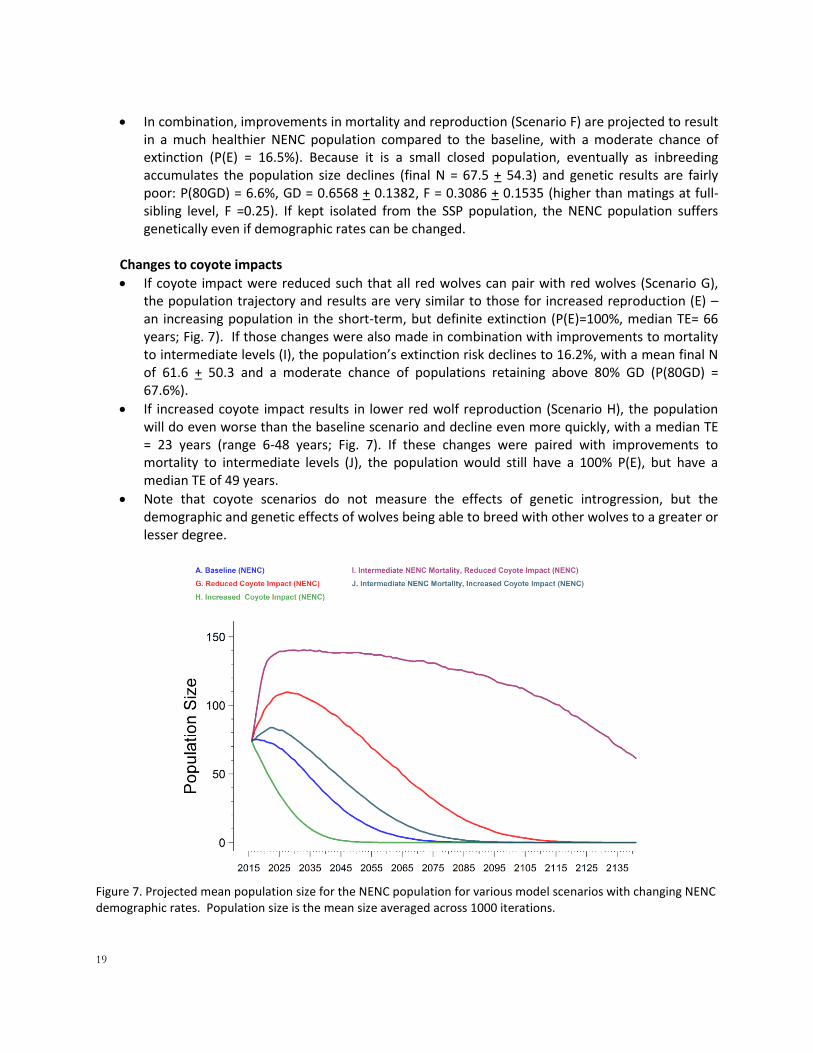
If coyote impact were reduced such that all red wolves can pair with red wolves (Scenario G), the population trajectory and results are very similar to those for increased reproduction (E) – an increasing population in the short-term, but definite extinction (P(E)=100%, median TE= 66 years; Fig. 7). If those changes were also made in combination with improvements to mortality to intermediate levels (I), the population’s extinction risk declines to 16.2%, with a mean final N of 61.6 + 50.3 and a moderate chance of populations retaining above 80% GD (P(80GD) = 67.6%).

If increased coyote impact results in lower red wolf reproduction (Scenario H), the population will do even worse than the baseline scenario and decline even more quickly, with a median TE = 23 years (range 6-48 years; Fig. 7). If these changes were paired with improvements to mortality to intermediate levels (J), the population would still have a 100% P(E), but have a median TE of 49 years.

Note that coyote scenarios do not measure the effects of genetic introgression, but the demographic and genetic effects of wolves being able to breed with other wolves to a greater or lesser degree.

Figure 7. Projected mean population size for the NENC population for various model scenarios with changing NENC demographic rates. Population size is the mean size averaged across 1000 iterations.

20

PVA Results – Scenarios With Changes to SSP Parameters The SSP population has the potential to be demographically strong, but additional space and improved breeding rates could substantially improve demographic and genetic outcomes.

As highlighted earlier, scenario FF illustrates that the SSP needs to increase births to avoid a decline; that increased breeding illustrated in the baseline scenario (A) will create a demographically stable population.

Increasing the SSP population size to the Recovery Plan target of 330 (Scenario K) or 400 (L) does not change the demographic outlook compared to the baseline scenario (A), but does result in substantial improvements in genetics – P(80GD) increases from 65.7% in the baseline to 80% at 330 wolves and 88.5% at 400 wolves, and final F decreases from 0.1799 + 0.0648 in the baseline to 0.1577 + 0.0508 at 330 wolves and 0.1496 + 0.0452 at 400 wolves. To reach these target sizes, the SSP would need to increase from making 52 pairs/year in the baseline (averaged over the first 10 model years) to ~76 pairs/year if 330 spaces were available, or ~82 pairs/year if 400 were available.

Coupling those changes with increased breeding success in the SSP (Scenarios M, N) results in additional improvements in genetics: P(80GD) = 88.3% at 330 wolves and 91.3% at 400 wolves, and final F is 0.1477 + 0.0459 at 330 wolves and 0.1426 + 0.0423 at 400 wolves. Under these scenarios, the SSP could make fewer pairs because success of individual pairs would be higher; if that pair success rate could be reached, the SSP would need to increase to ~62 pairs/year at 330 spaces (M) and ~75 pairs/year at 400 spaces (N).

PVA Results – SSP Population Absorbing NENC Wolves After NENC Termination If the decision were made to remove capturable NENC wolves from the current Recovery Area landscape and bring them into the SSP, it would not have a large impact on demographics of the SSP; genetically, the benefits of reintegrating NENC genes into the SSP would be greater if additional space is added to the SSP.

Bringing NENC animals might benefit the SSP population genetically, but much of that “extra” benefit would not be captured unless SSP population size was increased. Scenarios under current space (O) resulted in higher P(80GD), 71.4% compared to the baseline of 65.7%, but with additional spaces (P), much more GD could be captured, with P(80GD) = 87.1%. Thus adding space to the SSP if the NENC is terminated will be essential to avoid a permanent loss to the species’ genetic health. If additional spaces are not available, cryopreservation of genetic materials should be an important avenue for making sure NENC genes are captured, with investments in the research needed to utilize those genes via assisted reproduction.

The remaining NENC wolves that were not captured would persist until death; the modeled TE for the NENC population under these scenarios was 25 years (range 3-78 years).

21

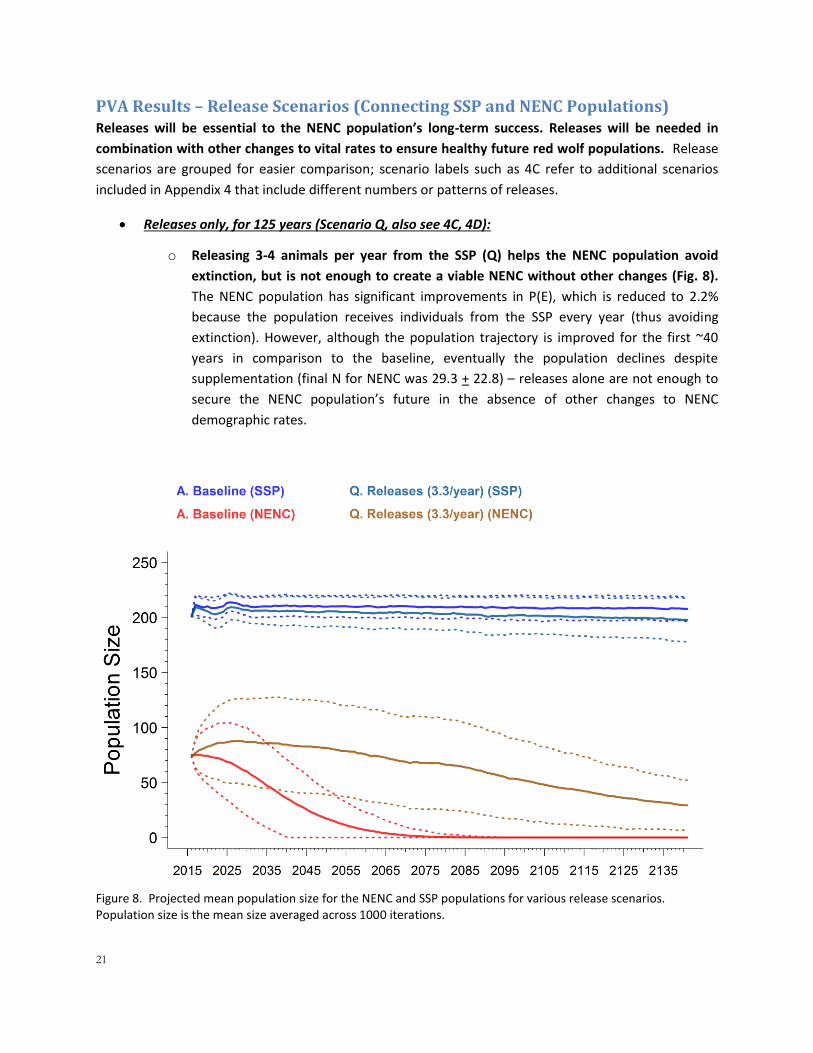
PVA Results – Release Scenarios (Connecting SSP and NENC Populations) Releases will be essential to the NENC population’s long-term success. Releases will be needed in

combination with other changes to vital rates to ensure healthy future red wolf populations. Release

scenarios are grouped for easier comparison; scenario labels such as 4C refer to additional scenarios

included in Appendix 4 that include different numbers or patterns of releases.

Releases only, for 125 years (Scenario Q, also see 4C, 4D):

o Releasing 3-4 animals per year from the SSP (Q) helps the NENC population avoid

extinction, but is not enough to create a viable NENC without other changes (Fig. 8).

The NENC population has significant improvements in P(E), which is reduced to 2.2%

because the population receives individuals from the SSP every year (thus avoiding

extinction). However, although the population trajectory is improved for the first ~40

years in comparison to the baseline, eventually the population declines despite

supplementation (final N for NENC was 29.3 + 22.8) – releases alone are not enough to

secure the NENC population’s future in the absence of other changes to NENC

demographic rates.

Figure 8. Projected mean population size for the NENC and SSP populations for various release scenarios. Population size is the mean size averaged across 1000 iterations.

22

o The SSP can sustain this release rate without major detrimental impacts on

demographics: final N = 197.2 + 20.0 in comparison to the baseline scenario (final N =

207.9). Releases do affect the SSP’s ability to remain above 80% GD, as the P(80GD)

decreases substantially from the baseline of 65.7% to 58.9% - harvesting animals

continuously for 125 years for the release program without changes to SSP rates may

have detrimental effects. However, in the model releases are randomly selected, and in

reality managers may have some ability to genetically select releases that are beneficial

to both the wild and SSP populations.

o Releases at higher rates (4-10 individuals per year in 4C, 4D) start to have detrimental

impacts on the SSP population without other changes. Releases of 9.6 animals per year

causes the SSP to decline (final N = 167.6 + 26.9), and the SSP is not able to produce

enough animals to release most model years.

Releases plus improvements to the SSP such as added space and improved reproduction

(Scenarios R, S, T, also see 4E, 4F, 4G):

o Adding more space to the SSP allows it to remain demographically strong and retain

higher GD while carrying out releases: With 3.3 wolves released for 125 years but

additional space (330, Scenario R, or 400 spaces, Scenario S), the SSP has large gains in

genetic health: it has P(80GD) of 78.1% with 330 spaces or 87.6% with 400 spaces,

substantially higher than the 58.9% chance of retaining 80% GD without any additional

space.

o Adding space and increasing SSP breeding to 25% (T) allows the SSP to retain the most

GD and to be the strongest source population for the NENC: With 3.3 wolves released

for 125 years, 400 spaces, and higher breeding (T), the SSP has the highest P(80GD) of

these set of scenarios, 92.8%, and the lowest F, 0.1412 + 0.0412 (compared to Scenario

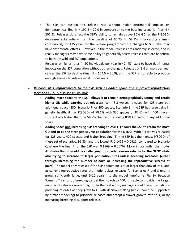
Q where the final F for the SSP was 0.1869 + 0.0676). More importantly, the model

illustrates that it would be challenging to provide releases reliably for the NENC while

also trying to increase to larger population sizes unless breeding increases (either

through increasing the number of pairs or increasing the reproductive success of

pairs). The model only releases if the SSP population is at or larger than 80% of its K, and

at current reproductive rates the model delays releases for Scenarios R and S until it

grows sufficiently large, until 5-10 years into the model timeframe (Fig. 9). Because

Scenario T ramps up breeding to fuel the growth to 400, it is able to provide the target

number of releases sooner (Fig. 9). In the real world, managers could carefully balance

providing releases as they grew to K, with decision-making (which could be supported

by further modeling) to prioritize releases and accept a slower growth rate to K, or by

increasing breeding to support releases.

23

Fig. 9. Projected mean number of releases from the SSP to the NENC population for various release scenarios.

Number of releases is the mean size averaged across only extant (surviving) iterations.

o The NENC population benefits from additional SSP space, and even more so from

space and increased SSP breeding. Although all 3 of these scenarios eventually settled

into the same number of animals for release after the first decade (Fig. 9), their early

dynamics are different and they do produce very different demographic and genetic

results in the NENC population. The NENC final N for Scenario Q (without SSP changes) is

29.3 + 22.8, while in R and S with increased space final N is 38.7 + 28.0 and 44.5 + 31.8,

respectively (Fig. 10). More importantly, these SSP changes have a substantial impact on

the genetics of the NENC. P(80GD) is only 34.3% for scenario Q, but 50.8% in R and

56.1% in S. If breeding is also increased in scenario T, P(80GD) is even higher at 60.6%.

These genetic differences exist even though the SSP is still sending the same number of

releases into the population because:

The SSP is genetically healthier at higher population sizes and breeding rates

(see results above), and because it can retain higher GD and lower F throughout

the simulation, it can release genetically healthier animals to the NENC (animals

that are less related to each other and to the rest of the NENC population).

Larger populations mean more genetic diversity is retained, and that retention

helps the NENC’s genetics as well

24

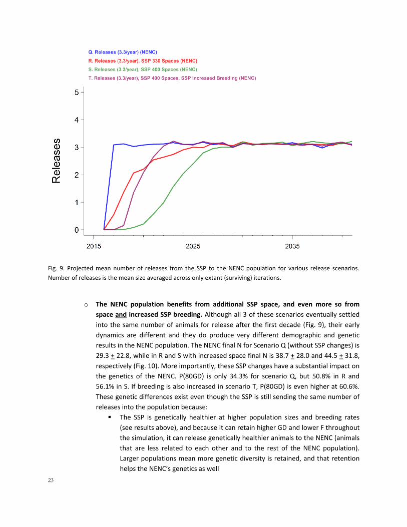
The NENC still experiences a demographic drag on its population as inbreeding

starts to accumulate under these scenarios, which translates into the

differences in population size; that drag is much less if the SSP is larger with

more breeding (Fig. 10). The NENC’s final F in scenario Q is 0.201 + 0.125; in

Scenario R and S, it is 0.175 (+ 0.102 or 0.099, respectively); in T, which

produces the best results demographically and genetically it is as low as 0.1577

+ 0.0879 (all still above that of mating of half siblings, where F = 0.125).

However, without changes to the NENC population’s vital rates, releases with

SSP improvements (more space, better breeding) are helpful but still cannot

counteract the NENC decline due to low survival and breeding rates and

inbreeding depression.

Figure 10. Mean final NENC population size for model scenarios with varying release strategies from the SSP to NENC population, and with additional space for the SSP. Mean size is calculated across all extant iterations. See Table 1 for scenario descriptions.

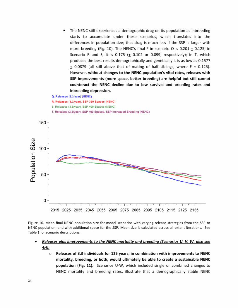
Releases plus improvements to the NENC mortality and breeding (Scenarios U, V, W, also see

4H):

o Releases of 3.3 individuals for 125 years, in combination with improvements to NENC

mortality, breeding, or both, would ultimately be able to create a sustainable NENC

population (Fig. 11). Scenarios U-W, which included single or combined changes to

NENC mortality and breeding rates, illustrate that a demographically stable NENC

25

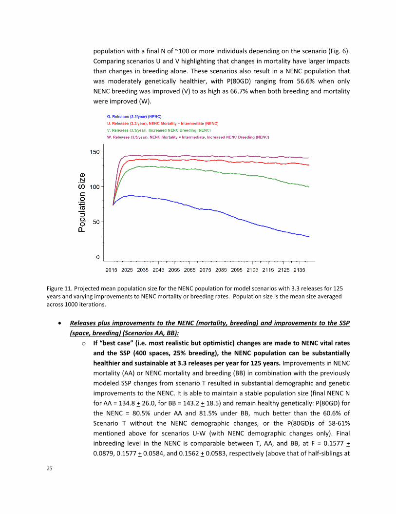
population with a final N of ~100 or more individuals depending on the scenario (Fig. 6).

Comparing scenarios U and V highlighting that changes in mortality have larger impacts

than changes in breeding alone. These scenarios also result in a NENC population that

was moderately genetically healthier, with P(80GD) ranging from 56.6% when only

NENC breeding was improved (V) to as high as 66.7% when both breeding and mortality

were improved (W).

Figure 11. Projected mean population size for the NENC population for model scenarios with 3.3 releases for 125 years and varying improvements to NENC mortality or breeding rates. Population size is the mean size averaged across 1000 iterations.

Releases plus improvements to the NENC (mortality, breeding) and improvements to the SSP

(space, breeding) (Scenarios AA, BB):

o If “best case” (i.e. most realistic but optimistic) changes are made to NENC vital rates

and the SSP (400 spaces, 25% breeding), the NENC population can be substantially

healthier and sustainable at 3.3 releases per year for 125 years. Improvements in NENC

mortality (AA) or NENC mortality and breeding (BB) in combination with the previously

modeled SSP changes from scenario T resulted in substantial demographic and genetic

improvements to the NENC. It is able to maintain a stable population size (final NENC N

for AA = 134.8 + 26.0, for BB = 143.2 + 18.5) and remain healthy genetically: P(80GD) for

the NENC = 80.5% under AA and 81.5% under BB, much better than the 60.6% of

Scenario T without the NENC demographic changes, or the P(80GD)s of 58-61%

mentioned above for scenarios U-W (with NENC demographic changes only). Final

inbreeding level in the NENC is comparable between T, AA, and BB, at F = 0.1577 +

0.0879, 0.1577 + 0.0584, and 0.1562 + 0.0583, respectively (above that of half-siblings at

26

0.125). These rates are lower than those mentioned above for U-W where NENC

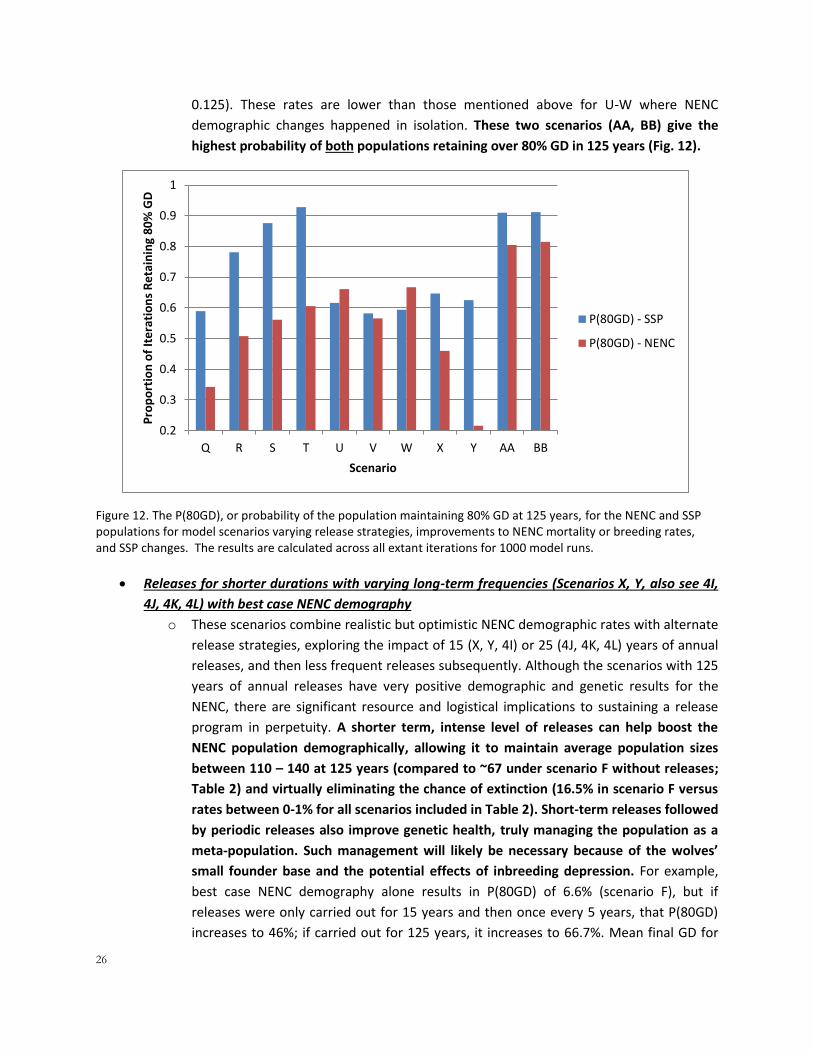
demographic changes happened in isolation. These two scenarios (AA, BB) give the

highest probability of both populations retaining over 80% GD in 125 years (Fig. 12).

Figure 12. The P(80GD), or probability of the population maintaining 80% GD at 125 years, for the NENC and SSP populations for model scenarios varying release strategies, improvements to NENC mortality or breeding rates, and SSP changes. The results are calculated across all extant iterations for 1000 model runs.

Releases for shorter durations with varying long-term frequencies (Scenarios X, Y, also see 4I,

4J, 4K, 4L) with best case NENC demography

o These scenarios combine realistic but optimistic NENC demographic rates with alternate

release strategies, exploring the impact of 15 (X, Y, 4I) or 25 (4J, 4K, 4L) years of annual

releases, and then less frequent releases subsequently. Although the scenarios with 125

years of annual releases have very positive demographic and genetic results for the

NENC, there are significant resource and logistical implications to sustaining a release

program in perpetuity. A shorter term, intense level of releases can help boost the

NENC population demographically, allowing it to maintain average population sizes

between 110 – 140 at 125 years (compared to ~67 under scenario F without releases;

Table 2) and virtually eliminating the chance of extinction (16.5% in scenario F versus

rates between 0-1% for all scenarios included in Table 2). Short-term releases followed

by periodic releases also improve genetic health, truly managing the population as a

meta-population. Such management will likely be necessary because of the wolves’

small founder base and the potential effects of inbreeding depression. For example,

best case NENC demography alone results in P(80GD) of 6.6% (scenario F), but if

releases were only carried out for 15 years and then once every 5 years, that P(80GD)

increases to 46%; if carried out for 125 years, it increases to 66.7%. Mean final GD for

0.2

0.3

0.4

0.5

0.6

0.7

0.8

0.9

1

Q R S T U V W X Y AA BB

Pro

po

rtio

n o

f It

era

tio

ns

Re

tain

ing

80

% G

D

Scenario

P(80GD) - SSP

P(80GD) - NENC

27

those scenarios is 0.6568 + 0.1382, 0.7794 + 0.0689, and 0.8127 + 0.051, respectively

(Table 2). Specific modeling targeted at evaluation of realistic release strategies may be

helpful in the future to evaluate tradeoffs for the species.

Table 2. Genetic and demographic results at 125 years for the NENC population related to scenarios with varying release strategies

NENC Population Results

N - Mean

N – SD

GD – Mean

GD – SD

F – mean

F - SD P(80)

F NENC mortality = intermediate, Increased females breeding NENC

67.46 54.29 0.6568 0.1382 0.3086 0.1535 0.066

W Movement (3.3 every year), NENC mortality = intermediate, NENC increased breeding

141.38 20.21 0.8127 0.0510 0.1755 0.0625 0.667

X Movement (3.3 per year for 15 years then every 5 years), NENC mortality = intermediate, NENC increased breeding

132.23 29.56 0.7794 0.0689 0.2078 0.0790 0.460

Y Movement (3.3 per year for 15 years then every 20 years), NENC mortality = intermediate, NENC increased breeding

113.62 43.54 0.7291 0.0952 0.2510 0.1103 0.216

4J Movement (3.3 per year for 25 years then every 5 years), NENC mortality = intermediate, NENC increased breeding

133.70 29.01 0.7760 0.0726 0.2117 0.0843 0.434

4K Movement (3.3 per year for 25 years then every 10 years), NENC mortality = intermediate, NENC increased breeding

127.94 34.45 0.7563 0.0828 0.2324 0.094 0.344

4L Movement (3.3 per year for 25 years then every 20 years), NENC mortality = intermediate, NENC increased breeding

115.40 40.68 0.7372 0.0929 0.2513 0.1092 0.262

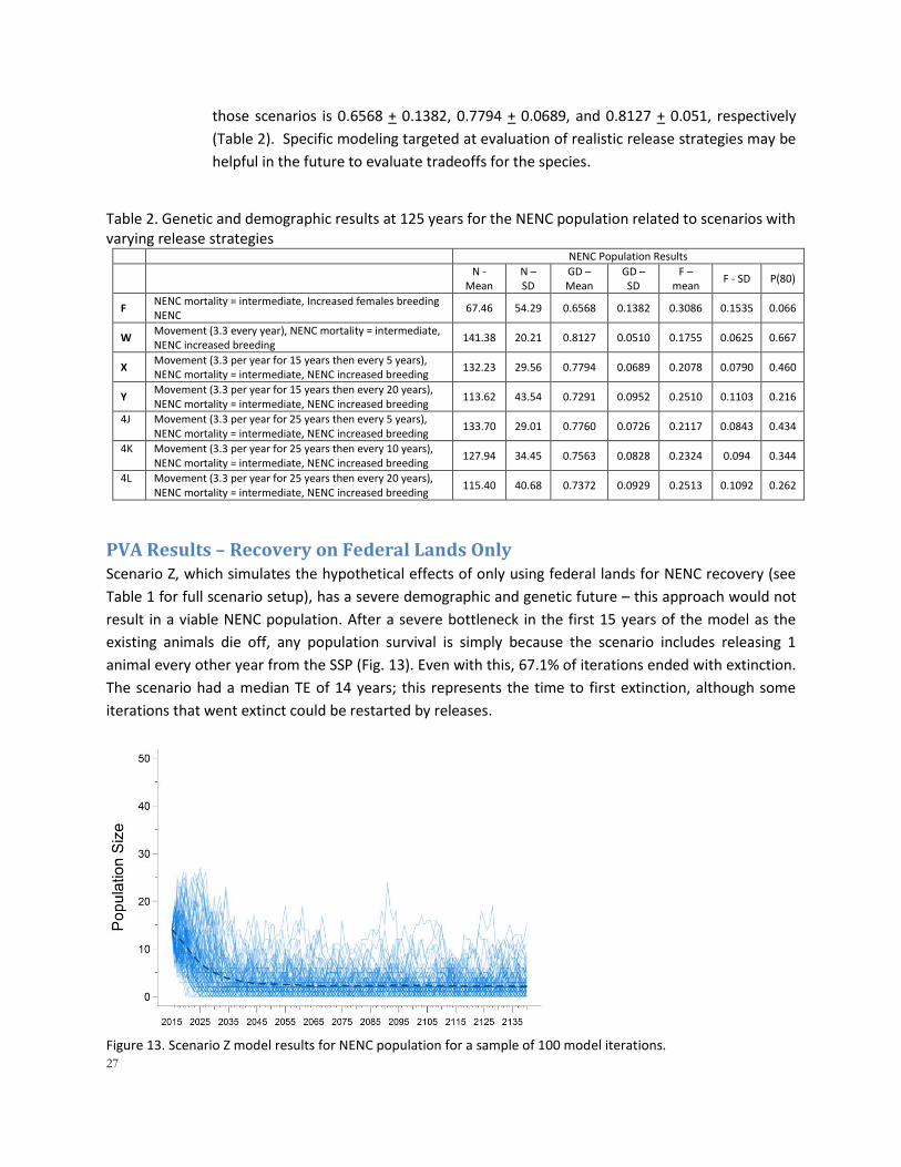
PVA Results – Recovery on Federal Lands Only Scenario Z, which simulates the hypothetical effects of only using federal lands for NENC recovery (see

Table 1 for full scenario setup), has a severe demographic and genetic future – this approach would not

result in a viable NENC population. After a severe bottleneck in the first 15 years of the model as the

existing animals die off, any population survival is simply because the scenario includes releasing 1

animal every other year from the SSP (Fig. 13). Even with this, 67.1% of iterations ended with extinction.

The scenario had a median TE of 14 years; this represents the time to first extinction, although some

iterations that went extinct could be restarted by releases.

Figure 13. Scenario Z model results for NENC population for a sample of 100 model iterations.

28

PVA Conclusions The overarching results from these modeling efforts indicate that:

1. Current conditions, without releases from the SSP or improvements to NENC vital rates, will result in extinction of the NENC population, typically within 37 years but in some iterations as soon as 8 years. The baseline NENC model is considered optimistic when compared to the current estimated population, which has already declined by an estimated 14-30 animals than our starting population taken as of 1 January 2015. Further, the model does not incorporate any requests to remove wolves from private land or more recent trends (2015 and 2016) in mortality and reproductive rates. These factors make it likely that 37 years is a high estimate of the time to extinction for the only remaining wild population of red wolves. This extinction would not just be about numbers, but would also represent the loss of behaviorally competent wild wolves on the landscape; creation of future populations at NENC or elsewhere would have to start from scratch and re-build that behavioral competence again, and would likely experience higher mortality and lower reproductive rates as it worked to re-build that competence.

2. The NENC population can avoid extinction and be viable, but requires assistance to do so:

a. There were several scenarios in which the NENC had less than 10% probability of extinction:

C NENC mortality = SSP mortality

D NENC mortality = Intermediate, no inbreeding depression

Q Movement (3.3 every year)

R Movement (3.3 every year), SSP 330 spaces

S Movement (3.3 every year), SSP 400 spaces

T Movement (3.3 every year), SSP 400 spaces, SSP 25% breeding

U Movement (3.3 every year), NENC mortality = intermediate

V Movement (3.3 every year), NENC increased breeding

W Movement (3.3 every year), NENC mortality = intermediate, NENC increased breeding

X Movement (3.3 per year for 15 years then every 5 years), NENC mortality = intermediate, NENC increased breeding

Y Movement (3.3 per year for 15 years then every 20 years), NENC mortality = intermediate, NENC increased breeding

AA Movement (3.3 every year), SSP 400 spaces, SSP 25% breeding, NENC mortality = intermediate

BB Movement (3.3 every year), SSP 400 spaces, SSP 25% breeding, NENC mortality = intermediate, NENC increased breeding

The most realistic of these are likely scenarios X or Y: a secure future with low extinction risk for the NENC can be created if the NENC can reduce its mortality closer to the modeled intermediate levels (which, when considered alone in scenario B, was a change from ~38 deaths to ~31 deaths in the first model year), increase breeding (by shifting mortality earlier in the year so its disruptive effect on breeding is reduced), and receive releases from the SSP for a short, intense period (15 years) followed by intermittent releases to maintain genetic health after that.

b. It will be challenging for the NENC population to have a strong probability (>80% chance) of retaining greater than 80% GD (when considered alone, separate from the SSP). Only two scenarios, AA and BB, were able to achieve that, and required NENC demographic changes, annual releases for 125 years, and SSP improvements (400

29

spaces and 25% breeding). This benchmark will likely be challenging for the NENC population alone to meet (but will be easier for the species as a whole to meet).

3. To remain a strong supporting population for any recovery goals, the SSP population needs the following changes to increase its viability:

a. Space: Model scenarios with growth to 330 or 400 spaces illustrate that the population could benefit substantially in its population genetics and ability to sustain releases from such a change - P(80GD) increases from 65.7% in the baseline to 80% at 330 wolves and 88.5% at 400 wolves. Currently, space limits population size and, because there are not enough spaces to place pups, fewer breeding recommendations are issued. This management results in the use of contraceptives, separating of pairs during the breeding season, and/or delayed or less frequent breeding opportunities for females. Evidence from other carnivore species suggests that all of these management actions can negatively impact female fertility and reproductive health (Penfold et al. 2014, Asa et al. 2014). Because data on these effects do not exist for red wolves, we did not explicitly model any of these effects, although it is possible that the rate of recommendation success (19%) is being partially driven by females experiencing fertility problems. To increase from 225 to a population size of 330 or 400 wolves, new resources would need to be identified. Space within AZA institutions is limited and there is “competition” for space with other large canids managed within AZA (e.g. Mexican gray wolf, maned wolf, gray wolf, etc.) and potential wolf spaces are often associated with an institution’s zoogeographic theme. The Red Wolf Species Survival Plan® (SSP) already has double the number of holding facilities (44) of similar AZA SSPs (median number of holding facilities is only 22 across all 324 “Yellow” SSPs; Yellow SSPs are populations with more than 50 animals that are not expected to retain 90% gene diversity for 100 years) and has long partnered with non-member facilities to expand beyond AZA institutions. Additional space to expand the captive population in facilities that exhibit animals to the public is limited. To hold 400 individual wolves, the SSP would likely need 100 more enclosures than now (Will Waddell, pers. comm.). The recent Canid and Hyaenid Integrated Collection Assessment and Planning (ICAP) process, which considered wild and captive populations of all canids and prioritized captive populations, recommended that the red wolf SSP population be expanded and that facilities consider converting spaces held by coyotes (and gray wolves) to red wolves if possible.

b. Reproductive improvements: Reproductive improvements are needed even if additional spaces aren’t available if the SSP wants to avoid demographic decline – Scenario A and FF in combination illustrate that an increase in the number of pairs made will be important to avoiding that decline. Another route to reproductive improvements could be making each pairing more successful (e.g. focusing on younger pairs, minimize delayed breeding in females), rather than just making additional pairs; if the pair success rate increased to 25% and the SSP had more space, it would result in even better genetic results: P(80GD) = 88.3% at 330 wolves and 91.3% at 400 wolves.

4. Both populations are small and will face rising inbreeding levels, and in model scenarios including the inbreeding effects that have already been detected (Appendix 1), population declines in the NENC will occur without changes to the NENC population’s demographic rates

30

and SSP releases. There is a possibility that some of these effects may lessen over time, if deleterious alleles are purged from the red wolf gene pool, but this amount of purging may be decreasing over time because the population’s small size means that genetic drift will override selective forces to purge. More work is needed to better understand the impact. Therefore, it is likely that the population will continue to see these inbreeding impacts. Genetic theory suggests that continuing to manage the population in the long-term as a metapopulation, with migrants (either animals or sperm) in both directions (SSP to NENC and NENC to SSP) to maximize and manage gene diversity and inbreeding in both populations, will likely be the best strategy to maintain the species’ long-term genetic health. In our model scenarios we did not include any genetic selection criteria for the releases that occurred, but in real time managers could plan breeding SSP pairs that would most benefit the NENC population genetically. The cross-fostering approach to releases is a promising management tool but has many logistical and timing constraints, which means that designed genetic selection is not predictable, but with additional space and increased breeding, the feasibility of this strategy is higher.

5. There are multiple ways to achieve the recovery goal of preserving at least 80% of the founding genetic diversity until 2140 when the species as a whole is considered (rather than the SSP and NENC considered separately). Scenarios which had greater than 80% chance of hitting that benchmark at the metapopulation level included:

C NENC mortality = SSP mortality

D NENC mortality = Intermediate, no inbreeding depression

F NENC mortality = intermediate, Increased females breeding NENC

I NENC mortality = intermediate, reduced coyote impact

L SSP 400 spaces

M SSP 330 spaces, SSP 25% breeding

N SSP 400 spaces, SSP 25% breeding

P Capturable wolves brought into SSP, SSP 330 spaces

S Movement (3.3 every year), SSP 400 spaces

T Movement (3.3 every year), SSP 400 spaces, SSP 25% breeding

X Movement (3.3 per year for 15 years then every 5 years), NENC mortality = intermediate, NENC increased breeding

Y Movement (3.3 per year for 15 years then every 20 years), NENC mortality = intermediate, NENC increased breeding

AA Movement (3.3 every year), SSP 400 spaces, SSP 25% breeding, NENC mortality = intermediate

BB Movement (3.3 every year), SSP 400 spaces, SSP 25% breeding, NENC mortality = intermediate, NENC increased breeding

4B Capturable wolves brought into SSP, SSP 400 spaces

4E Movement (young, 4.5 per year), SSP 330 spaces

4F Movement (young, 4.5 per year), SSP 400 spaces

4G Movement (young, 4.5 per year), SSP 400 spaces, SSP 25% breeding

4I Movement (3.3 per year for 15 years then every 10 years), NENC mortality = intermediate, NENC increased breeding

4J Movement (3.3 per year for 25 years then every 5 years), NENC mortality = intermediate, NENC increased breeding

4K Movement (3.3 per year for 25 years then every 10 years), NENC mortality = intermediate, NENC increased breeding

4L Movement (3.3 per year for 25 years then every 20 years), NENC mortality = intermediate, NENC increased breeding

31

These modeling scenarios highlight that red wolves will be a conservation-reliant species, requiring population management: all red wolves will need to be treated as a metapopulation, with occasional movement between the SSP and NENC, and perhaps other populations if they are established, to manage declining gene diversity given its small founding population (Goble et al. 2012). However, with NENC demographic changes and releases, maintaining a functioning wild NENC population is possible. This is a key example of a species that can be best preserved by the “One Plan” approach, where all populations, captive and wild, are considered under an integrated plan for species conservation (Byers et al. 2013).

32

Appendix 1: Vortex Model Setup Documentation & Supporting Analyses This Appendix details the set-up of the metapopulation model of the red wolf (Canis rufus) constructed for the Red Wolf Feasibility Assessment. The model was constructed and evaluated using the program Vortex 10 (specific version: 10.1.4.0) (www.vortex.org). This model and supporting analyses were developed by Dr. Joseph (Josie) L. Simonis of DAPPER, LLC as a member of and in collaboration with the Red Wolf Population Viability Analysis Team. The full model file may be made available on request, and/or will be archived with later publication of this research.

Sections

1. Data Sources 2. Conceptual Models for Baseline Scenario 3. Model Setup and Supporting Analyses 4. Figures 5. Tables

1. Data Sources Data for the red wolf population and its management were collected from the SSP Studbook (Waddell 2015), the US Fish and Wildlife Red Wolf Population Database (USFWS, unpublished data), and PMCTrack (www.PMCTrack.org) (Faust et al. 2015). For the SSP population, following standard methodology, “modern management” was considered 1 January 1980 – 31 December 2014 (Simonis et al. 2015a). Thus, in general, that time frame was used for SSP data. However, more recent tracking of the SSP process has generated management data from 2001 onward (e.g., Table A1). Thus, for some analyses, a restricted time window is used for the SSP. For the NENC population, while the database goes all the way back to the initiation of the population, more intensive data collection was begun in 2000, allowing for much more rigorous data regarding, for example, mate pairs. A date window of 1 January 2000 – 31 December 2014 was used for all analyses unless otherwise noted.

33

2. Conceptual Models for Baseline Scenario

To better document and illustrate how we have used Vortex to model the dynamics of both the SSP and NENC populations, we created conceptual models of modeled dynamics for both populations:

34

3. MODEL SETUP AND SUPPORTING ANALYSES

Minor Model Variables and Assumptions

We are assuming that there is concordance between environmental variation in reproduction and survival, such that “good years” and “bad years” for survival are directly correlated with good and bad years for reproduction.

We are assuming that there is no correlation in environmental variation between the NENC and SSP populations (i.e., a good year in the NENC does not necessarily translate to a good year in the SSP).

We are assuming that reproduction is not density-dependent in either the SSP or NENC.

35

When animals move between the SSP and NENC via Vortex’s Harvest and Supplementation routines, there is no additional mortality caused by the movement itself, and animals instantly take on the survival and reproductive rates of the NENC.

Model order of events: our modeled order is different from the default in Vortex 10. In particular, Dispersal has been removed (not being used) and Harvest and Supplement have been moved ahead of Mortality and Age, which allows us to move pups between the populations in the way that wolves are actually managed (right after birth via fostering). First year mortality is delayed until all litters are produced (rather than directly after the creation of each litter), which allows very young pups to be moved (as is needed for pup fostering) before mortality occurs:

Event Type Explanation EV Environmental Variation is imposed Breed Reproduction Harvest As translocation: removal from SSP Supplement As translocation: release to NENC Mortality Mortality (all age classes) Age Animals age +1 year rCalc Calculate population growth rate Ktruncation Enforce Carrying Capacity UpdateVars Update State Variables Census Census the population

Offspring Sex Ratio

Supporting Analysis:

We analyzed the impact of inbreeding on the birth sex ratio of captive and NENC red wolves. In total, we included 1765 total pups: 904 females (51.2%) and 861 males (48.8%). We removed unknown sex individuals. The inbreeding values of the individuals included ranged from 0 to 0.341, with median = 0.076, mean = 0.088, and standard deviation = 0.068. In total, 749 pups were from the NENC (42.4%), and 1016 were from SSP (57.6%). We used a logistic regression (generalized linear model with logit link), using the pup’s inbreeding value and population to predict the sex. We also included blocking factors associated with dam and litter, but neither explained any variation in the sex ratio of offspring, and so they were excluded.

The birth sex ratio is significantly impacted by the inbreeding value of the pup, such that it is male biased with increasing inbreeding level (p = 0.04). There is no significant difference in the birth sex ratio between the SSP and NENC population (p = 0.34). See Fig. A1. Using the general logistic relationship

𝐵𝑆𝑅 =𝑒(𝑏0+𝑏1×𝐼)

𝑒(𝑏0+𝑏1×𝐼) + 1

where BSR = Birth Sex Ratio (1.0 = Male, 0.0 = Female), I = inbreeding of the pup, and 𝑏0 and 𝑏1 are the intercept and slope (respectively), which are fitted statistically. Coefficient Estimate SE(estimate) p Intercept (𝑏0) -0.17462 0.07786 0.0249

36

Slope (𝑏1) 1.43362 0.70165 0.0410 Using the point estimates, the current population level median inbreeding (0.089) generates a BSR of 0.488 (48.8% males). A 50:50 sex ratio is achieved with an inbreeding value of ~0.12. Baseline Model Setup: The final model uses an equation of:

𝐵𝑆𝑅 =𝑒(−0.175+1.434×𝐼)

𝑒(−0.175+1.434×𝐼) + 1

where BSR = Birth Sex Ratio (1.0 = Male, 0.0 = Female) and I = inbreeding of the pup Alternate Scenario Setup: For the “no inbreeding impact” scenarios, we set the parameters equal to the inbreeding equation evaluated at the relevant population’s current median inbreeding level (SSP: 0.075, NENC: 0.113, Total: 0.089).

Birth Sex Ratio (BSR; 1.0 = Male, 0.0 = Female):

𝐵𝑆𝑅 =𝑒(−0.175+1.434×0.089)

𝑒(−0.175+1.434×0.089) + 1= 0.488

Litter size

Supporting Analysis: We analyzed the impact of inbreeding on litter size in captive and NENC red wolves. In total, our data set included 373 litters, 127 of which were NENC-born (2000-2015) and 246 of which were captive-born (1980-2015). Kinship between parents (i.e., the inbreeding value of the pups) ranged from 0 to 0.341 (median = 0.075, mean = 0.090, standard deviation = 0.073). We used a Poisson regression (generalized linear model with log link), and evaluated the impact of kinship between parents and population on the litter size. The data are well-approximated by a Poisson distribution, except from the lack of 0s. However, mean litter size is large enough (4.19) that the probability mass of 0 is only 0.015 (relatively infrequent). The data are slightly overdispersed, but not excessively so: as the variance (4.52) is only 1.08 times the mean (4.19). Litter size decreases significantly with increasing kinship between parents (p = 0.0001) and is significantly larger in the NENC population (p = 0.0005) (Fig. A2, A10). Using the general log relationship

𝐿𝑆 = 𝑒𝑏0+𝑏1+𝑏2×𝐾𝐼𝑁 where LS = Litter Size, KIN = kinship between parents, and 𝑏0, 𝑏1, and 𝑏2 are the general intercept, the population effect, and slope (respectively), which are fitted statistically.

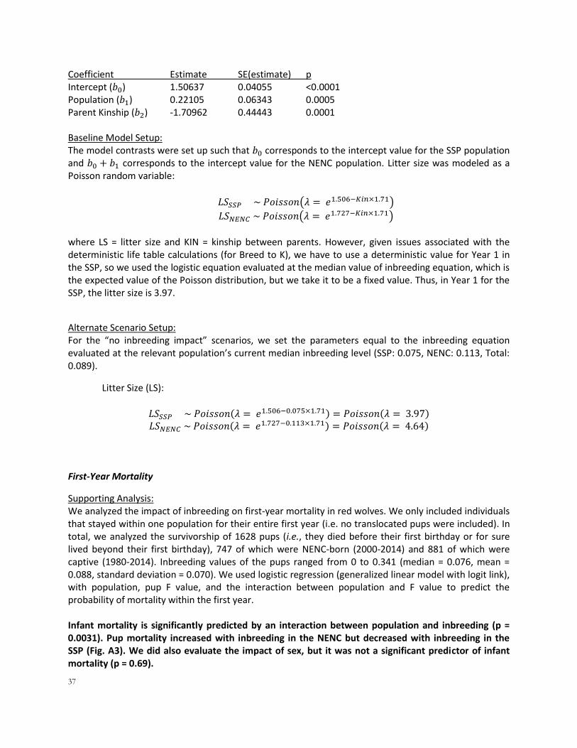
37

Coefficient Estimate SE(estimate) p Intercept (𝑏0) 1.50637 0.04055 <0.0001 Population (𝑏1) 0.22105 0.06343 0.0005 Parent Kinship (𝑏2) -1.70962 0.44443 0.0001 Baseline Model Setup: The model contrasts were set up such that 𝑏0 corresponds to the intercept value for the SSP population and 𝑏0 + 𝑏1 corresponds to the intercept value for the NENC population. Litter size was modeled as a Poisson random variable:

𝐿𝑆𝑆𝑆𝑃 ~ 𝑃𝑜𝑖𝑠𝑠𝑜𝑛(𝜆 = 𝑒1.506−𝐾𝑖𝑛×1.71)

𝐿𝑆𝑁𝐸𝑁𝐶 ~ 𝑃𝑜𝑖𝑠𝑠𝑜𝑛(𝜆 = 𝑒1.727−𝐾𝑖𝑛×1.71)

where LS = litter size and KIN = kinship between parents. However, given issues associated with the deterministic life table calculations (for Breed to K), we have to use a deterministic value for Year 1 in the SSP, so we used the logistic equation evaluated at the median value of inbreeding equation, which is the expected value of the Poisson distribution, but we take it to be a fixed value. Thus, in Year 1 for the SSP, the litter size is 3.97.

Alternate Scenario Setup: For the “no inbreeding impact” scenarios, we set the parameters equal to the inbreeding equation evaluated at the relevant population’s current median inbreeding level (SSP: 0.075, NENC: 0.113, Total: 0.089).

Litter Size (LS):

𝐿𝑆𝑆𝑆𝑃 ~ 𝑃𝑜𝑖𝑠𝑠𝑜𝑛(𝜆 = 𝑒1.506−0.075×1.71) = 𝑃𝑜𝑖𝑠𝑠𝑜𝑛(𝜆 = 3.97) 𝐿𝑆𝑁𝐸𝑁𝐶 ~ 𝑃𝑜𝑖𝑠𝑠𝑜𝑛(𝜆 = 𝑒1.727−0.113×1.71) = 𝑃𝑜𝑖𝑠𝑠𝑜𝑛(𝜆 = 4.64)

First-Year Mortality

Supporting Analysis: We analyzed the impact of inbreeding on first-year mortality in red wolves. We only included individuals that stayed within one population for their entire first year (i.e. no translocated pups were included). In total, we analyzed the survivorship of 1628 pups (i.e., they died before their first birthday or for sure lived beyond their first birthday), 747 of which were NENC-born (2000-2014) and 881 of which were captive (1980-2014). Inbreeding values of the pups ranged from 0 to 0.341 (median = 0.076, mean = 0.088, standard deviation = 0.070). We used logistic regression (generalized linear model with logit link), with population, pup F value, and the interaction between population and F value to predict the probability of mortality within the first year. Infant mortality is significantly predicted by an interaction between population and inbreeding (p = 0.0031). Pup mortality increased with inbreeding in the NENC but decreased with inbreeding in the SSP (Fig. A3). We did also evaluate the impact of sex, but it was not a significant predictor of infant mortality (p = 0.69).

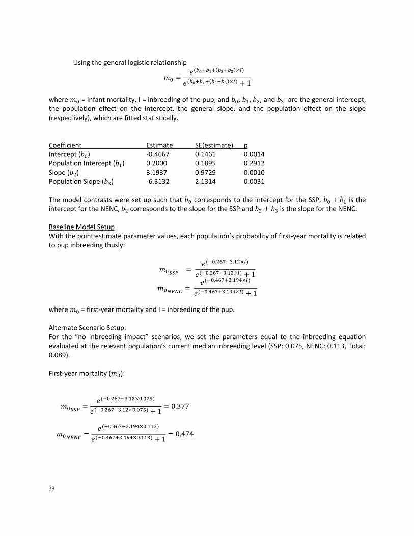
38

Using the general logistic relationship

𝑚0 =𝑒(𝑏0+𝑏1+(𝑏2+𝑏3)×𝐼)

𝑒(𝑏0+𝑏1+(𝑏2+𝑏3)×𝐼) + 1

where 𝑚0 = infant mortality, I = inbreeding of the pup, and 𝑏0, 𝑏1, 𝑏2, and 𝑏3 are the general intercept, the population effect on the intercept, the general slope, and the population effect on the slope (respectively), which are fitted statistically. Coefficient Estimate SE(estimate) p Intercept (𝑏0) -0.4667 0.1461 0.0014 Population Intercept (𝑏1) 0.2000 0.1895 0.2912 Slope (𝑏2) 3.1937 0.9729 0.0010 Population Slope (𝑏3) -6.3132 2.1314 0.0031 The model contrasts were set up such that 𝑏0 corresponds to the intercept for the SSP, 𝑏0 + 𝑏1 is the intercept for the NENC, 𝑏2 corresponds to the slope for the SSP and 𝑏2 + 𝑏3 is the slope for the NENC. Baseline Model Setup With the point estimate parameter values, each population’s probability of first-year mortality is related to pup inbreeding thusly:

𝑚0𝑆𝑆𝑃 =

𝑒(−0.267−3.12×𝐼)

𝑒(−0.267−3.12×𝐼) + 1

𝑚0𝑁𝐸𝑁𝐶=

𝑒(−0.467+3.194×𝐼)

𝑒(−0.467+3.194×𝐼) + 1

where 𝑚0 = first-year mortality and I = inbreeding of the pup. Alternate Scenario Setup: For the “no inbreeding impact” scenarios, we set the parameters equal to the inbreeding equation evaluated at the relevant population’s current median inbreeding level (SSP: 0.075, NENC: 0.113, Total: 0.089). First-year mortality (𝑚0):

𝑚0𝑆𝑆𝑃=

𝑒(−0.267−3.12×0.075)

𝑒(−0.267−3.12×0.075) + 1= 0.377

𝑚0𝑁𝐸𝑁𝐶=

𝑒(−0.467+3.194×0.113)

𝑒(−0.467+3.194×0.113) + 1= 0.474

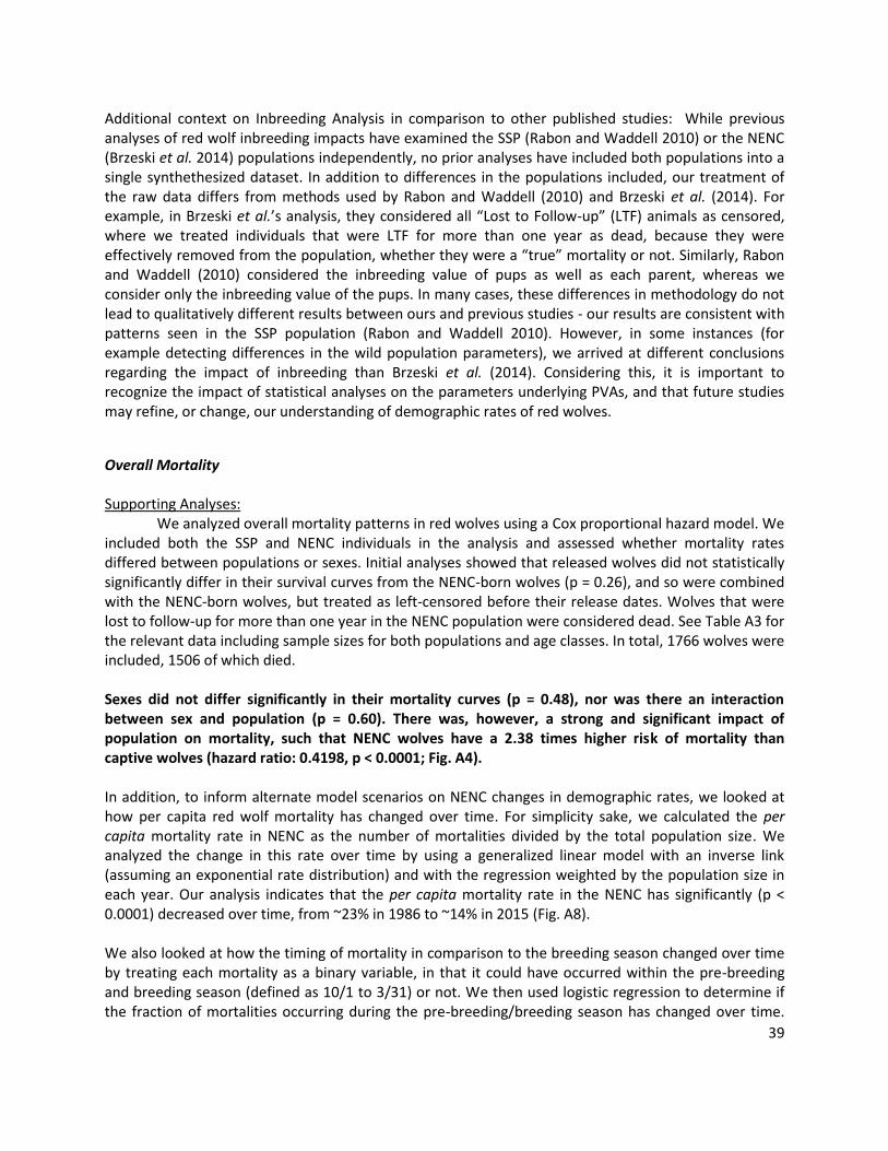
39

Additional context on Inbreeding Analysis in comparison to other published studies: While previous analyses of red wolf inbreeding impacts have examined the SSP (Rabon and Waddell 2010) or the NENC (Brzeski et al. 2014) populations independently, no prior analyses have included both populations into a single synthethesized dataset. In addition to differences in the populations included, our treatment of the raw data differs from methods used by Rabon and Waddell (2010) and Brzeski et al. (2014). For example, in Brzeski et al.’s analysis, they considered all “Lost to Follow-up” (LTF) animals as censored, where we treated individuals that were LTF for more than one year as dead, because they were effectively removed from the population, whether they were a “true” mortality or not. Similarly, Rabon and Waddell (2010) considered the inbreeding value of pups as well as each parent, whereas we consider only the inbreeding value of the pups. In many cases, these differences in methodology do not lead to qualitatively different results between ours and previous studies - our results are consistent with patterns seen in the SSP population (Rabon and Waddell 2010). However, in some instances (for example detecting differences in the wild population parameters), we arrived at different conclusions regarding the impact of inbreeding than Brzeski et al. (2014). Considering this, it is important to recognize the impact of statistical analyses on the parameters underlying PVAs, and that future studies may refine, or change, our understanding of demographic rates of red wolves.

Overall Mortality Supporting Analyses: We analyzed overall mortality patterns in red wolves using a Cox proportional hazard model. We included both the SSP and NENC individuals in the analysis and assessed whether mortality rates differed between populations or sexes. Initial analyses showed that released wolves did not statistically significantly differ in their survival curves from the NENC-born wolves (p = 0.26), and so were combined with the NENC-born wolves, but treated as left-censored before their release dates. Wolves that were lost to follow-up for more than one year in the NENC population were considered dead. See Table A3 for the relevant data including sample sizes for both populations and age classes. In total, 1766 wolves were included, 1506 of which died. Sexes did not differ significantly in their mortality curves (p = 0.48), nor was there an interaction between sex and population (p = 0.60). There was, however, a strong and significant impact of population on mortality, such that NENC wolves have a 2.38 times higher risk of mortality than captive wolves (hazard ratio: 0.4198, p < 0.0001; Fig. A4). In addition, to inform alternate model scenarios on NENC changes in demographic rates, we looked at how per capita red wolf mortality has changed over time. For simplicity sake, we calculated the per capita mortality rate in NENC as the number of mortalities divided by the total population size. We analyzed the change in this rate over time by using a generalized linear model with an inverse link (assuming an exponential rate distribution) and with the regression weighted by the population size in each year. Our analysis indicates that the per capita mortality rate in the NENC has significantly (p < 0.0001) decreased over time, from ~23% in 1986 to ~14% in 2015 (Fig. A8). We also looked at how the timing of mortality in comparison to the breeding season changed over time by treating each mortality as a binary variable, in that it could have occurred within the pre-breeding and breeding season (defined as 10/1 to 3/31) or not. We then used logistic regression to determine if the fraction of mortalities occurring during the pre-breeding/breeding season has changed over time.

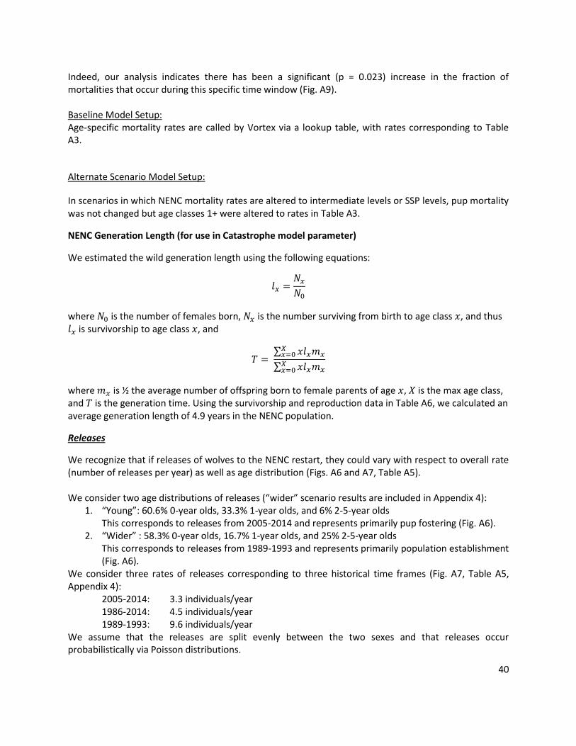
40

Indeed, our analysis indicates there has been a significant (p = 0.023) increase in the fraction of mortalities that occur during this specific time window (Fig. A9). Baseline Model Setup: Age-specific mortality rates are called by Vortex via a lookup table, with rates corresponding to Table A3.

Alternate Scenario Model Setup:

In scenarios in which NENC mortality rates are altered to intermediate levels or SSP levels, pup mortality was not changed but age classes 1+ were altered to rates in Table A3.

NENC Generation Length (for use in Catastrophe model parameter)

We estimated the wild generation length using the following equations:

𝑙𝑥 =𝑁𝑥

𝑁0

where 𝑁0 is the number of females born, 𝑁𝑥 is the number surviving from birth to age class 𝑥, and thus 𝑙𝑥 is survivorship to age class 𝑥, and

𝑇 = ∑ 𝑥𝑙𝑥𝑚𝑥

𝑋𝑥=0

∑ 𝑥𝑙𝑥𝑚𝑥𝑋𝑥=0

where 𝑚𝑥 is ½ the average number of offspring born to female parents of age 𝑥, 𝑋 is the max age class, and 𝑇 is the generation time. Using the survivorship and reproduction data in Table A6, we calculated an average generation length of 4.9 years in the NENC population.

Releases

We recognize that if releases of wolves to the NENC restart, they could vary with respect to overall rate (number of releases per year) as well as age distribution (Figs. A6 and A7, Table A5). We consider two age distributions of releases (“wider” scenario results are included in Appendix 4):

1. “Young”: 60.6% 0-year olds, 33.3% 1-year olds, and 6% 2-5-year olds This corresponds to releases from 2005-2014 and represents primarily pup fostering (Fig. A6).

2. “Wider” : 58.3% 0-year olds, 16.7% 1-year olds, and 25% 2-5-year olds This corresponds to releases from 1989-1993 and represents primarily population establishment (Fig. A6).

We consider three rates of releases corresponding to three historical time frames (Fig. A7, Table A5, Appendix 4):

2005-2014: 3.3 individuals/year 1986-2014: 4.5 individuals/year

1989-1993: 9.6 individuals/year We assume that the releases are split evenly between the two sexes and that releases occur probabilistically via Poisson distributions.

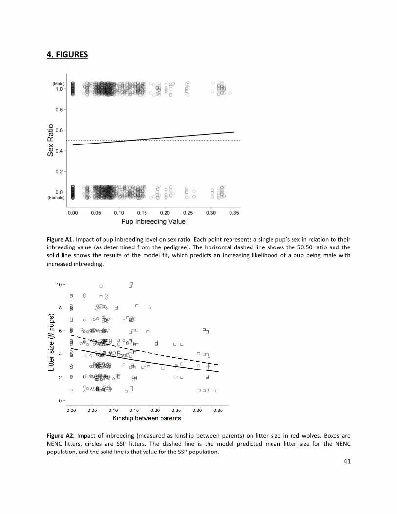
41

4. FIGURES

Figure A1. Impact of pup inbreeding level on sex ratio. Each point represents a single pup’s sex in relation to their inbreeding value (as determined from the pedigree). The horizontal dashed line shows the 50:50 ratio and the solid line shows the results of the model fit, which predicts an increasing likelihood of a pup being male with

increased inbreeding.

Figure A2. Impact of inbreeding (measured as kinship between parents) on litter size in red wolves. Boxes are NENC litters, circles are SSP litters. The dashed line is the model predicted mean litter size for the NENC population, and the solid line is that value for the SSP population.

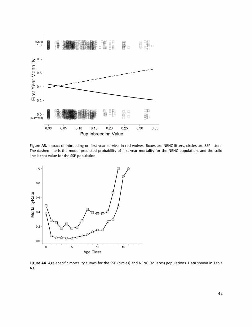
42

Figure A3. Impact of inbreeding on first year survival in red wolves. Boxes are NENC litters, circles are SSP litters. The dashed line is the model predicted probability of first year mortality for the NENC population, and the solid line is that value for the SSP population.

Figure A4. Age-specific mortality curves for the SSP (circles) and NENC (squares) populations. Data shown in Table A3.

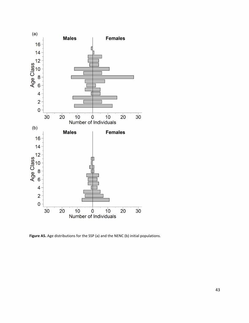
43

Figure A5. Age distributions for the SSP (a) and the NENC (b) initial populations.

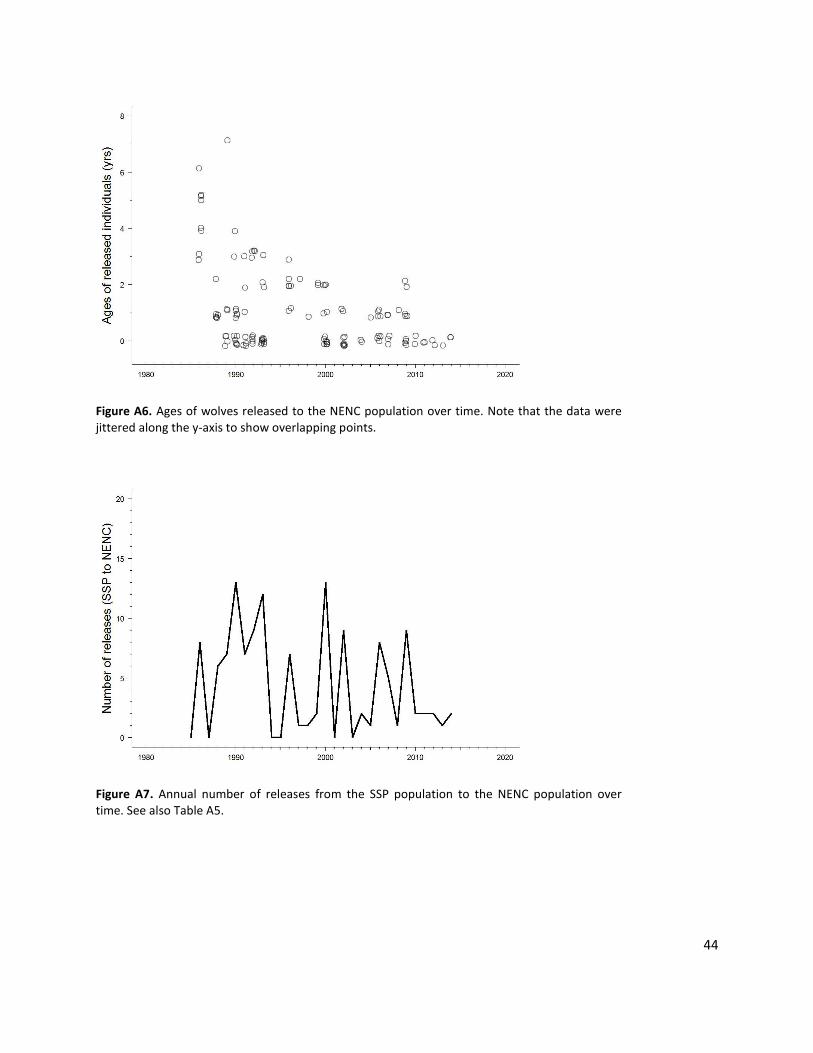
44

Figure A6. Ages of wolves released to the NENC population over time. Note that the data were jittered along the y-axis to show overlapping points.

Figure A7. Annual number of releases from the SSP population to the NENC population over time. See also Table A5.

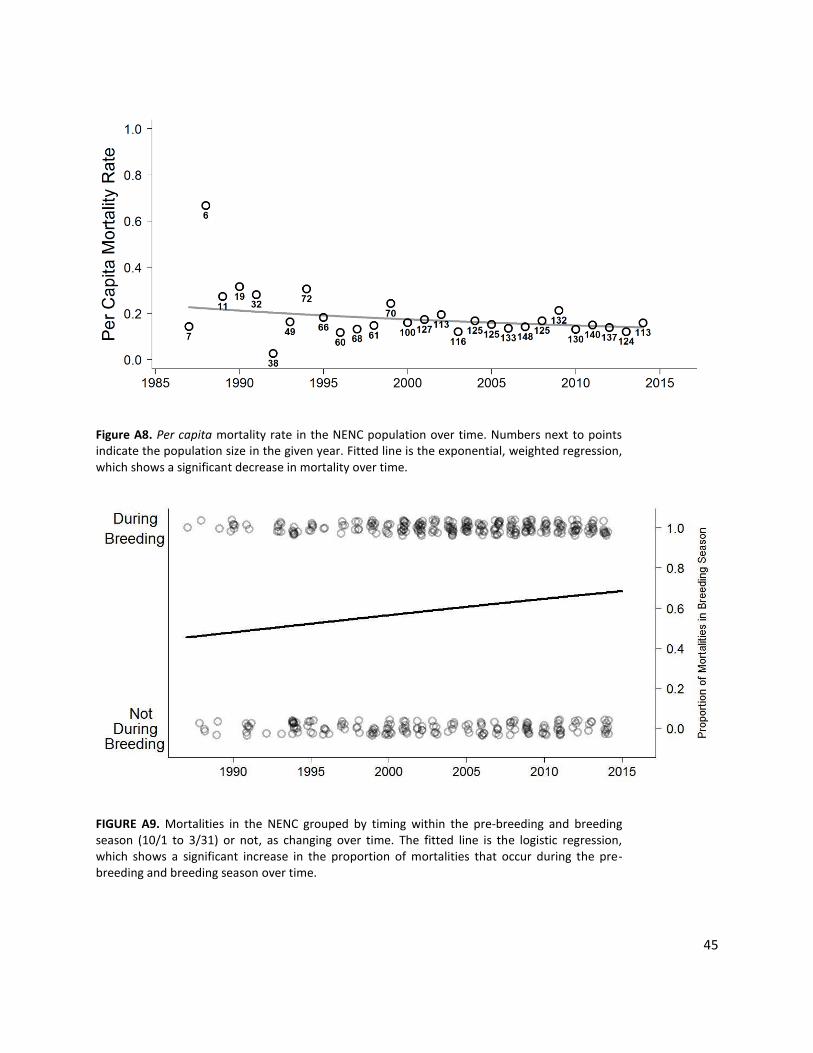
45

Figure A8. Per capita mortality rate in the NENC population over time. Numbers next to points indicate the population size in the given year. Fitted line is the exponential, weighted regression, which shows a significant decrease in mortality over time.

FIGURE A9. Mortalities in the NENC grouped by timing within the pre-breeding and breeding season (10/1 to 3/31) or not, as changing over time. The fitted line is the logistic regression, which shows a significant increase in the proportion of mortalities that occur during the pre-breeding and breeding season over time.

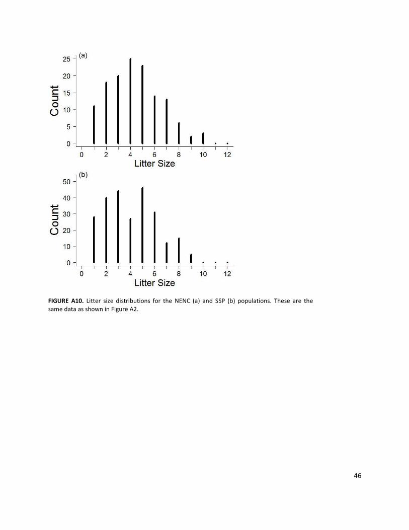
46

FIGURE A10. Litter size distributions for the NENC (a) and SSP (b) populations. These are the same data as shown in Figure A2.

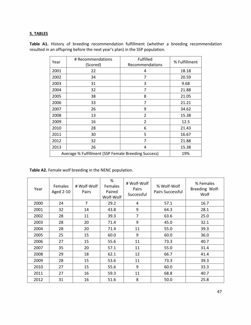
47

5. TABLES

Table A1. History of breeding recommendation fulfillment (whether a breeding recommendation resulted in an offspring before the next year’s plan) in the SSP population.

Year # Recommendations

(Scored) Fulfilled

Recommendations % Fulfillment

2001 22 4 18.18

2002 34 7 20.59

2003 31 3 9.68

2004 32 7 21.88

2005 38 8 21.05

2006 33 7 21.21

2007 26 9 34.62

2008 13 2 15.38

2009 16 2 12.5

2010 28 6 21.43

2011 30 5 16.67

2012 32 7 21.88

2013 26 4 15.38

Average % Fulfillment (SSP Female Breeding Success) 19%

Table A2. Female wolf breeding in the NENC population.

Year Females

Aged 2-10 # Wolf-Wolf

Pairs

% Females Paired

Wolf-Wolf

# Wolf-Wolf Pairs

Successful

% Wolf-Wolf Pairs Successful

% Females Breeding Wolf-

Wolf

2000 24 7 29.2 4 57.1 16.7

2001 32 14 43.8 9 64.3 28.1

2002 28 11 39.3 7 63.6 25.0

2003 28 20 71.4 9 45.0 32.1

2004 28 20 71.4 11 55.0 39.3

2005 25 15 60.0 9 60.0 36.0

2006 27 15 55.6 11 73.3 40.7

2007 35 20 57.1 11 55.0 31.4

2008 29 18 62.1 12 66.7 41.4

2009 28 15 53.6 11 73.3 39.3

2010 27 15 55.6 9 60.0 33.3

2011 27 16 59.3 11 68.8 40.7

2012 31 16 51.6 8 50.0 25.8

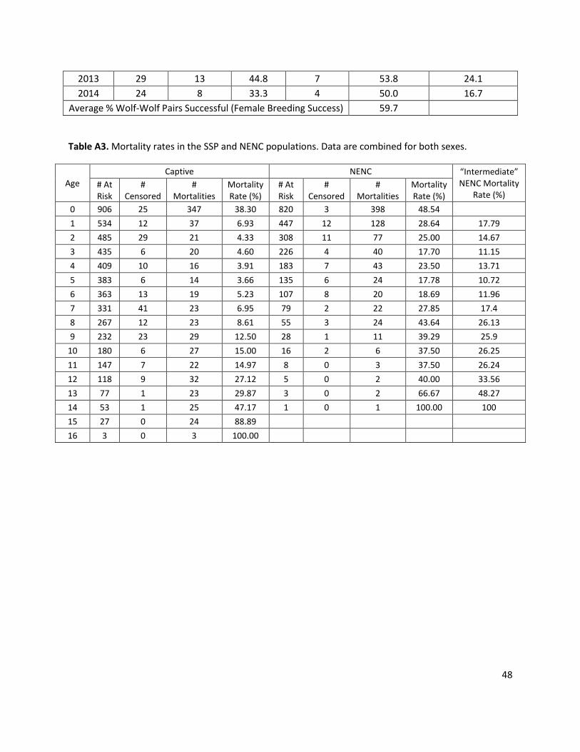
48

2013 29 13 44.8 7 53.8 24.1

2014 24 8 33.3 4 50.0 16.7

Average % Wolf-Wolf Pairs Successful (Female Breeding Success) 59.7

Table A3. Mortality rates in the SSP and NENC populations. Data are combined for both sexes.

Age

Captive NENC “Intermediate” NENC Mortality

Rate (%) # At Risk

# Censored

# Mortalities

Mortality Rate (%)

# At Risk

# Censored

# Mortalities

Mortality Rate (%)

0 906 25 347 38.30 820 3 398 48.54

1 534 12 37 6.93 447 12 128 28.64 17.79

2 485 29 21 4.33 308 11 77 25.00 14.67

3 435 6 20 4.60 226 4 40 17.70 11.15

4 409 10 16 3.91 183 7 43 23.50 13.71

5 383 6 14 3.66 135 6 24 17.78 10.72

6 363 13 19 5.23 107 8 20 18.69 11.96

7 331 41 23 6.95 79 2 22 27.85 17.4

8 267 12 23 8.61 55 3 24 43.64 26.13

9 232 23 29 12.50 28 1 11 39.29 25.9

10 180 6 27 15.00 16 2 6 37.50 26.25

11 147 7 22 14.97 8 0 3 37.50 26.24

12 118 9 32 27.12 5 0 2 40.00 33.56

13 77 1 23 29.87 3 0 2 66.67 48.27

14 53 1 25 47.17 1 0 1 100.00 100

15 27 0 24 88.89

16 3 0 3 100.00

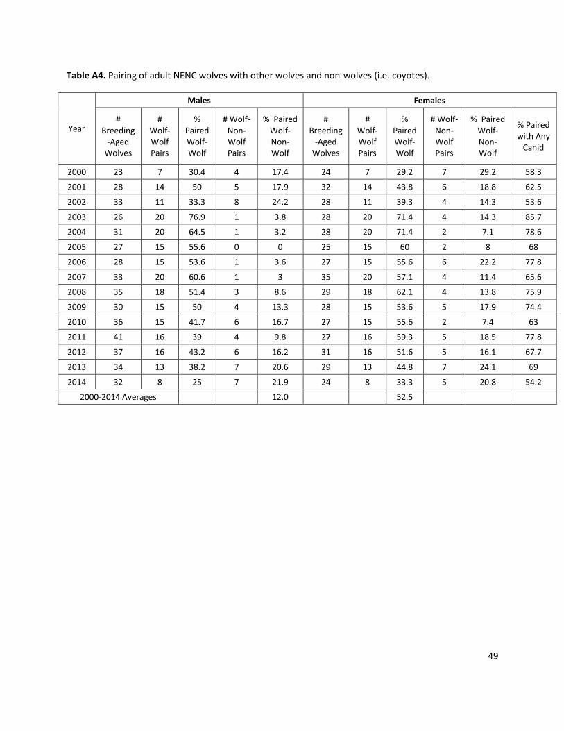
49

Table A4. Pairing of adult NENC wolves with other wolves and non-wolves (i.e. coyotes).

Year

Males Females

# Breeding

-Aged Wolves

# Wolf-Wolf Pairs

% Paired Wolf-Wolf

# Wolf-Non-Wolf Pairs

% Paired Wolf-Non-Wolf

# Breeding

-Aged Wolves

# Wolf-Wolf Pairs

% Paired Wolf-Wolf

# Wolf-Non-Wolf Pairs

% Paired Wolf-Non-Wolf

% Paired with Any

Canid

2000 23 7 30.4 4 17.4 24 7 29.2 7 29.2 58.3

2001 28 14 50 5 17.9 32 14 43.8 6 18.8 62.5

2002 33 11 33.3 8 24.2 28 11 39.3 4 14.3 53.6

2003 26 20 76.9 1 3.8 28 20 71.4 4 14.3 85.7

2004 31 20 64.5 1 3.2 28 20 71.4 2 7.1 78.6

2005 27 15 55.6 0 0 25 15 60 2 8 68

2006 28 15 53.6 1 3.6 27 15 55.6 6 22.2 77.8

2007 33 20 60.6 1 3 35 20 57.1 4 11.4 65.6

2008 35 18 51.4 3 8.6 29 18 62.1 4 13.8 75.9

2009 30 15 50 4 13.3 28 15 53.6 5 17.9 74.4

2010 36 15 41.7 6 16.7 27 15 55.6 2 7.4 63

2011 41 16 39 4 9.8 27 16 59.3 5 18.5 77.8

2012 37 16 43.2 6 16.2 31 16 51.6 5 16.1 67.7

2013 34 13 38.2 7 20.6 29 13 44.8 7 24.1 69

2014 32 8 25 7 21.9 24 8 33.3 5 20.8 54.2

2000-2014 Averages 12.0 52.5

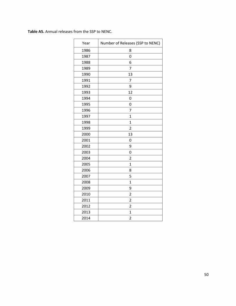
50

Table A5. Annual releases from the SSP to NENC.

Year Number of Releases (SSP to NENC)

1986 8

1987 0

1988 6

1989 7

1990 13

1991 7

1992 9

1993 12

1994 0

1995 0

1996 7

1997 1

1998 1

1999 2

2000 13

2001 0

2002 9

2003 0

2004 2

2005 1

2006 8

2007 5

2008 1

2009 9

2010 2

2011 2

2012 2

2013 1

2014 2

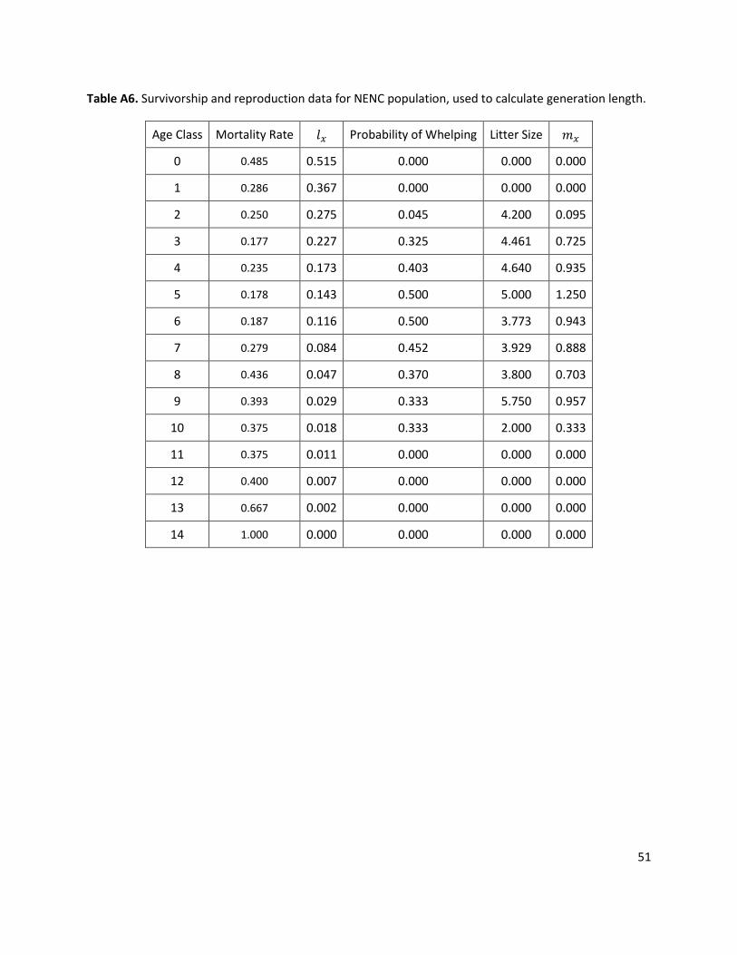
51

Table A6. Survivorship and reproduction data for NENC population, used to calculate generation length.

Age Class Mortality Rate 𝑙𝑥 Probability of Whelping Litter Size 𝑚𝑥

0 0.485 0.515 0.000 0.000 0.000

1 0.286 0.367 0.000 0.000 0.000

2 0.250 0.275 0.045 4.200 0.095

3 0.177 0.227 0.325 4.461 0.725

4 0.235 0.173 0.403 4.640 0.935

5 0.178 0.143 0.500 5.000 1.250

6 0.187 0.116 0.500 3.773 0.943

7 0.279 0.084 0.452 3.929 0.888

8 0.436 0.047 0.370 3.800 0.703

9 0.393 0.029 0.333 5.750 0.957

10 0.375 0.018 0.333 2.000 0.333

11 0.375 0.011 0.000 0.000 0.000

12 0.400 0.007 0.000 0.000 0.000

13 0.667 0.002 0.000 0.000 0.000

14 1.000 0.000 0.000 0.000 0.000

52

Appendix 2. Model Scenario Results Table Abbreviation Description

P(E) Probability of extinction in 125 years (i.e. the # of extinct iterations/total # of iterations)

GD Mean gene diversity in 125 years, calculated across surviving (non-extinct) model iterations

F Mean inbreeding coefficient in 125 years, calculated across surviving (non-extinct) model iterations

N Mean population size in 125 years, calculated across 1000 model iterations (extinct and extant)

TE Median time to extinction for iterations that go extinct (only reported if the population went extinct in at least 50% of simulations)

P(80GD) Probability of population maintaining 80% GD at 125 years, calculated across all surviving (non-extinct) model iterations

SSP RESULTS:

Label

Scenario Name

SSP

N P (E)

TE GD F P (80GD) Mean SD Median Mean SD Mean SD

A Baseline 207.93 11.44 0 -- 0.8100 0.0536 0.1799 0.0648 0.657

B NENC mortality = intermediate 208.20 11.27 0 -- 0.8132 0.0509 0.1748 0.0593 0.690

C NENC mortality = SSP mortality 207.82 12.09 0 -- 0.8070 0.0545 0.1788 0.0638 0.635

D NENC mortality = Intermediate, no inbreeding depression

208.98 10.20 0 -- 0.8107 0.0522 0.1790 0.0627 0.656

E Increased females breeding NENC 207.84 12.43 0 -- 0.8092 0.0505 0.1803 0.0613 0.657

F NENC mortality = intermediate, Increased females breeding NENC

207.79 11.50 0 -- 0.8112 0.0526 0.1779 0.0623 0.695

G Reduced coyote impact 208.18 11.86 0 -- 0.8088 0.0543 0.1793 0.0674 0.654

H Increased coyote impact 208.09 12.49 0 -- 0.8096 0.0509 0.1788 0.0595 0.661

I NENC mortality = intermediate, reduced coyote impact

207.41 11.65 0 -- 0.8099 0.0530 0.1796 0.0640 0.676

J NENC mortality = intermediate, Increased coyote impact

207.90 10.87 0 -- 0.8074 0.0583 0.1820 0.0671 0.647

K SSP 330 spaces 308.97 11.21 0 -- 0.8334 0.0437 0.1577 0.0508 0.800

L SSP 400 spaces 375.24 12.57 0 -- 0.8437 0.039 0.1496 0.0452 0.885

M SSP 330 spaces, SSP 25% breeding 310.47 10.82 0 -- 0.8453 0.0387 0.1477 0.0459 0.883

N SSP 400 spaces, SSP 25% breeding 376.09 11.69 0 -- 0.8511 0.0362 0.1426 0.0423 0.913

O Capturable wolves brought into SSP

209.31 10.40 0 -- 0.8168 0.0535 0.1710 0.0629 0.714

P Capturable wolves brought into SSP, SSP 330 spaces

309.06 11.86 0 -- 0.8435 0.0418 0.1501 0.0497 0.871

Q Movement (3.3 every year) 197.85 20.01 0 -- 0.8007 0.0547 0.1869 0.0676 0.589

R Movement (3.3 every year), SSP 330 spaces

304.55 14.44 0 -- 0.8287 0.0463 0.1648 0.0538 0.781

S Movement (3.3 every year), SSP 400 spaces

371.99 13.79 0 -- 0.8421 0.0397 0.1509 0.0464 0.876

T Movement (3.3 every year), SSP 400 spaces, SSP 25% breeding

374.23 12.37 0 -- 0.8524 0.0356 0.1412 0.0412 0.928

U Movement (3.3 every year), NENC mortality = intermediate

198.61 18.23 0 -- 0.8025 0.0582 0.1846 0.0701 0.616

V Movement (3.3 every year), NENC increased breeding

198.14 19.48 0 -- 0.8003 0.0565 0.1880 0.0675 0.582

W Movement (3.3 every year), NENC 197.70 19.52 0 -- 0.8008 0.0571 0.1885 0.0678 0.594

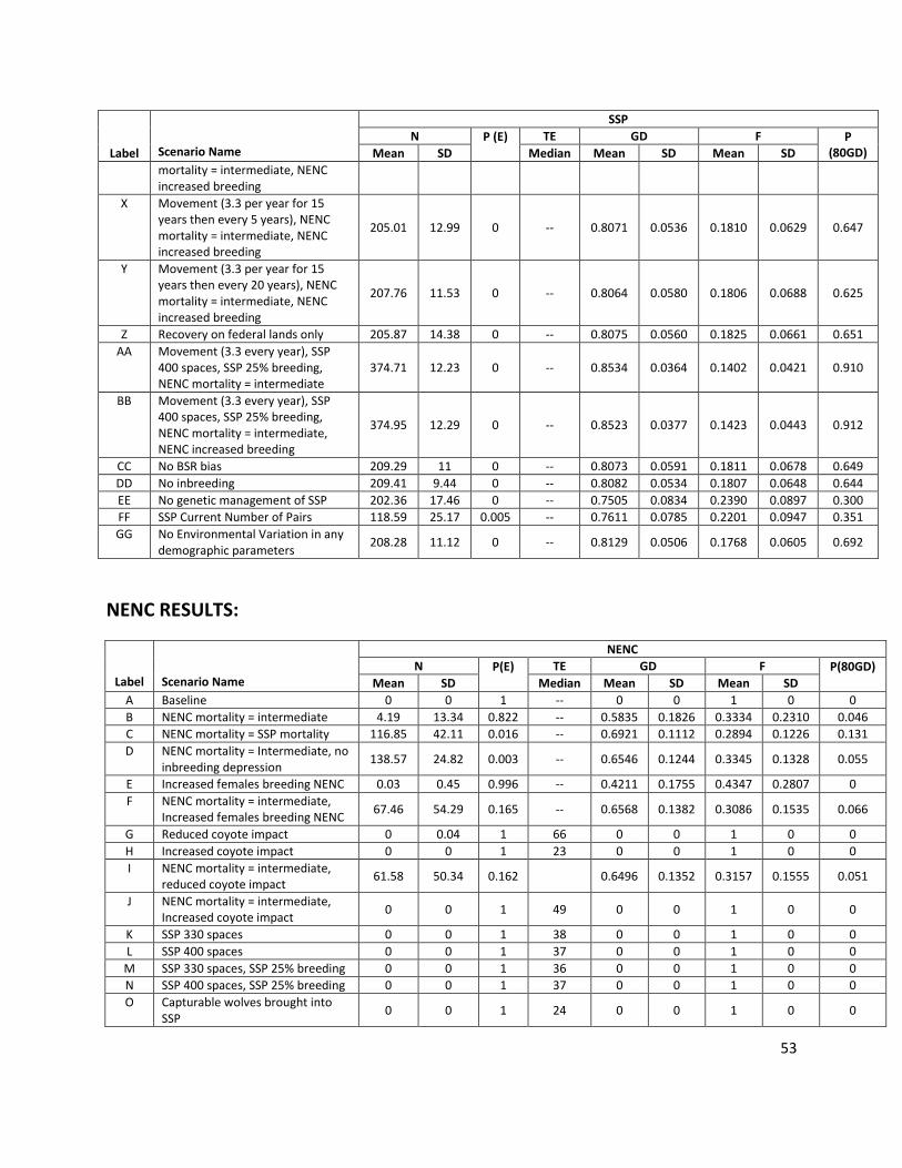
53

Label

Scenario Name

SSP

N P (E)

TE GD F P (80GD) Mean SD Median Mean SD Mean SD

mortality = intermediate, NENC increased breeding

X Movement (3.3 per year for 15 years then every 5 years), NENC mortality = intermediate, NENC increased breeding

205.01 12.99 0 -- 0.8071 0.0536 0.1810 0.0629 0.647

Y Movement (3.3 per year for 15 years then every 20 years), NENC mortality = intermediate, NENC increased breeding

207.76 11.53 0 -- 0.8064 0.0580 0.1806 0.0688 0.625

Z Recovery on federal lands only 205.87 14.38 0 -- 0.8075 0.0560 0.1825 0.0661 0.651

AA Movement (3.3 every year), SSP 400 spaces, SSP 25% breeding, NENC mortality = intermediate

374.71 12.23 0 -- 0.8534 0.0364 0.1402 0.0421 0.910

BB Movement (3.3 every year), SSP 400 spaces, SSP 25% breeding, NENC mortality = intermediate, NENC increased breeding

374.95 12.29 0 -- 0.8523 0.0377 0.1423 0.0443 0.912

CC No BSR bias 209.29 11 0 -- 0.8073 0.0591 0.1811 0.0678 0.649

DD No inbreeding 209.41 9.44 0 -- 0.8082 0.0534 0.1807 0.0648 0.644

EE No genetic management of SSP 202.36 17.46 0 -- 0.7505 0.0834 0.2390 0.0897 0.300

FF SSP Current Number of Pairs 118.59 25.17 0.005 -- 0.7611 0.0785 0.2201 0.0947 0.351

GG No Environmental Variation in any demographic parameters

208.28 11.12 0 -- 0.8129 0.0506 0.1768 0.0605 0.692

NENC RESULTS:

Label

Scenario Name

NENC

N P(E)

TE GD F P(80GD) Mean SD Median Mean SD Mean SD

A Baseline 0 0 1 -- 0 0 1 0 0

B NENC mortality = intermediate 4.19 13.34 0.822 -- 0.5835 0.1826 0.3334 0.2310 0.046

C NENC mortality = SSP mortality 116.85 42.11 0.016 -- 0.6921 0.1112 0.2894 0.1226 0.131

D NENC mortality = Intermediate, no inbreeding depression

138.57 24.82 0.003 -- 0.6546 0.1244 0.3345 0.1328 0.055

E Increased females breeding NENC 0.03 0.45 0.996 -- 0.4211 0.1755 0.4347 0.2807 0

F NENC mortality = intermediate, Increased females breeding NENC

67.46 54.29 0.165 -- 0.6568 0.1382 0.3086 0.1535 0.066

G Reduced coyote impact 0 0.04 1 66 0 0 1 0 0

H Increased coyote impact 0 0 1 23 0 0 1 0 0

I NENC mortality = intermediate, reduced coyote impact

61.58 50.34 0.162

0.6496 0.1352 0.3157 0.1555 0.051

J NENC mortality = intermediate, Increased coyote impact

0 0 1 49 0 0 1 0 0

K SSP 330 spaces 0 0 1 38 0 0 1 0 0

L SSP 400 spaces 0 0 1 37 0 0 1 0 0

M SSP 330 spaces, SSP 25% breeding 0 0 1 36 0 0 1 0 0

N SSP 400 spaces, SSP 25% breeding 0 0 1 37 0 0 1 0 0

O Capturable wolves brought into SSP

0 0 1 24 0 0 1 0 0

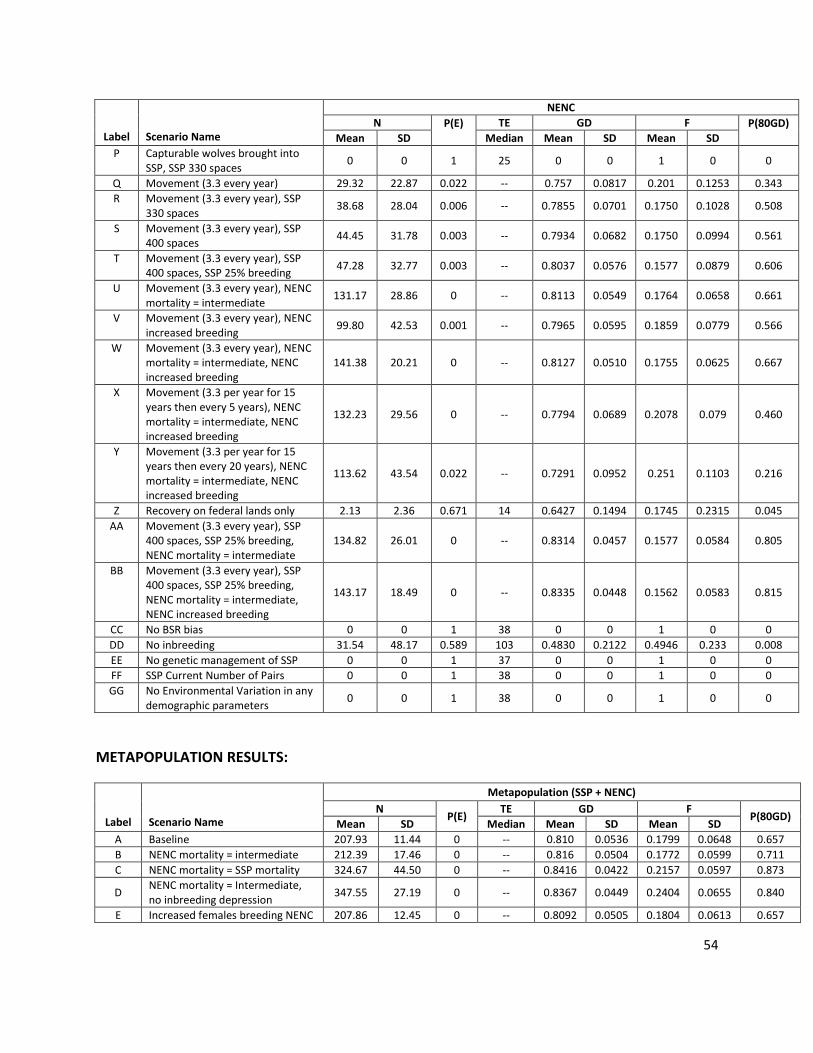
54

Label

Scenario Name

NENC

N P(E)

TE GD F P(80GD) Mean SD Median Mean SD Mean SD

P Capturable wolves brought into SSP, SSP 330 spaces

0 0 1 25 0 0 1 0 0

Q Movement (3.3 every year) 29.32 22.87 0.022 -- 0.757 0.0817 0.201 0.1253 0.343

R Movement (3.3 every year), SSP 330 spaces

38.68 28.04 0.006 -- 0.7855 0.0701 0.1750 0.1028 0.508

S Movement (3.3 every year), SSP 400 spaces

44.45 31.78 0.003 -- 0.7934 0.0682 0.1750 0.0994 0.561

T Movement (3.3 every year), SSP 400 spaces, SSP 25% breeding

47.28 32.77 0.003 -- 0.8037 0.0576 0.1577 0.0879 0.606

U Movement (3.3 every year), NENC mortality = intermediate

131.17 28.86 0 -- 0.8113 0.0549 0.1764 0.0658 0.661

V Movement (3.3 every year), NENC increased breeding

99.80 42.53 0.001 -- 0.7965 0.0595 0.1859 0.0779 0.566

W Movement (3.3 every year), NENC mortality = intermediate, NENC increased breeding

141.38 20.21 0 -- 0.8127 0.0510 0.1755 0.0625 0.667

X Movement (3.3 per year for 15 years then every 5 years), NENC mortality = intermediate, NENC increased breeding

132.23 29.56 0 -- 0.7794 0.0689 0.2078 0.079 0.460

Y Movement (3.3 per year for 15 years then every 20 years), NENC mortality = intermediate, NENC increased breeding

113.62 43.54 0.022 -- 0.7291 0.0952 0.251 0.1103 0.216

Z Recovery on federal lands only 2.13 2.36 0.671 14 0.6427 0.1494 0.1745 0.2315 0.045

AA Movement (3.3 every year), SSP 400 spaces, SSP 25% breeding, NENC mortality = intermediate

134.82 26.01 0 -- 0.8314 0.0457 0.1577 0.0584 0.805

BB Movement (3.3 every year), SSP 400 spaces, SSP 25% breeding, NENC mortality = intermediate, NENC increased breeding

143.17 18.49 0 -- 0.8335 0.0448 0.1562 0.0583 0.815

CC No BSR bias 0 0 1 38 0 0 1 0 0

DD No inbreeding 31.54 48.17 0.589 103 0.4830 0.2122 0.4946 0.233 0.008

EE No genetic management of SSP 0 0 1 37 0 0 1 0 0

FF SSP Current Number of Pairs 0 0 1 38 0 0 1 0 0

GG No Environmental Variation in any demographic parameters

0 0 1 38 0 0 1 0 0

METAPOPULATION RESULTS:

Label

Scenario Name

Metapopulation (SSP + NENC)

N P(E)

TE GD F P(80GD)

Mean SD Median Mean SD Mean SD

A Baseline 207.93 11.44 0 -- 0.810 0.0536 0.1799 0.0648 0.657

B NENC mortality = intermediate 212.39 17.46 0 -- 0.816 0.0504 0.1772 0.0599 0.711

C NENC mortality = SSP mortality 324.67 44.50 0 -- 0.8416 0.0422 0.2157 0.0597 0.873

D NENC mortality = Intermediate, no inbreeding depression

347.55 27.19 0 -- 0.8367 0.0449 0.2404 0.0655 0.840

E Increased females breeding NENC 207.86 12.45 0 -- 0.8092 0.0505 0.1804 0.0613 0.657

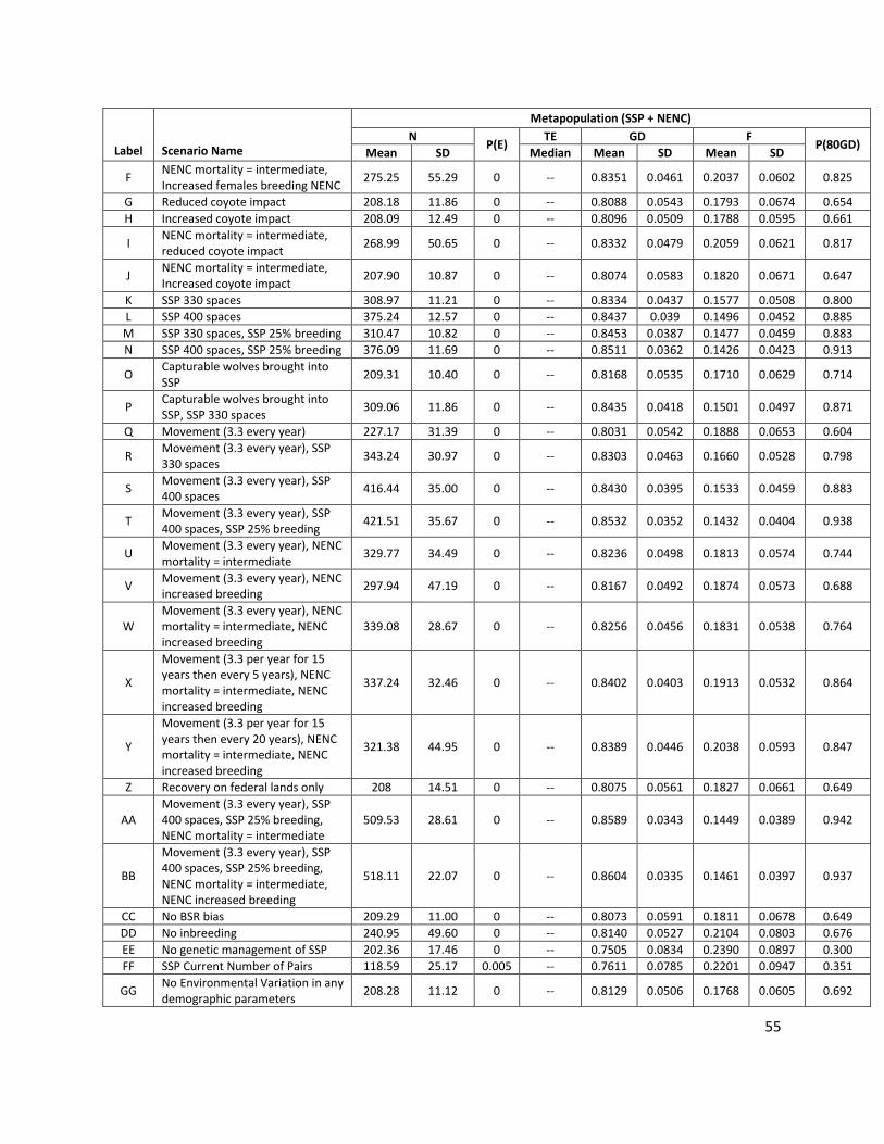
55

Label

Scenario Name

Metapopulation (SSP + NENC)

N P(E)

TE GD F P(80GD)

Mean SD Median Mean SD Mean SD

F NENC mortality = intermediate, Increased females breeding NENC

275.25 55.29 0 -- 0.8351 0.0461 0.2037 0.0602 0.825

G Reduced coyote impact 208.18 11.86 0 -- 0.8088 0.0543 0.1793 0.0674 0.654

H Increased coyote impact 208.09 12.49 0 -- 0.8096 0.0509 0.1788 0.0595 0.661

I NENC mortality = intermediate, reduced coyote impact

268.99 50.65 0 -- 0.8332 0.0479 0.2059 0.0621 0.817

J NENC mortality = intermediate, Increased coyote impact

207.90 10.87 0 -- 0.8074 0.0583 0.1820 0.0671 0.647

K SSP 330 spaces 308.97 11.21 0 -- 0.8334 0.0437 0.1577 0.0508 0.800

L SSP 400 spaces 375.24 12.57 0 -- 0.8437 0.039 0.1496 0.0452 0.885

M SSP 330 spaces, SSP 25% breeding 310.47 10.82 0 -- 0.8453 0.0387 0.1477 0.0459 0.883

N SSP 400 spaces, SSP 25% breeding 376.09 11.69 0 -- 0.8511 0.0362 0.1426 0.0423 0.913

O Capturable wolves brought into SSP

209.31 10.40 0 -- 0.8168 0.0535 0.1710 0.0629 0.714

P Capturable wolves brought into SSP, SSP 330 spaces

309.06 11.86 0 -- 0.8435 0.0418 0.1501 0.0497 0.871

Q Movement (3.3 every year) 227.17 31.39 0 -- 0.8031 0.0542 0.1888 0.0653 0.604

R Movement (3.3 every year), SSP 330 spaces

343.24 30.97 0 -- 0.8303 0.0463 0.1660 0.0528 0.798

S Movement (3.3 every year), SSP 400 spaces

416.44 35.00 0 -- 0.8430 0.0395 0.1533 0.0459 0.883

T Movement (3.3 every year), SSP 400 spaces, SSP 25% breeding

421.51 35.67 0 -- 0.8532 0.0352 0.1432 0.0404 0.938

U Movement (3.3 every year), NENC mortality = intermediate

329.77 34.49 0 -- 0.8236 0.0498 0.1813 0.0574 0.744

V Movement (3.3 every year), NENC increased breeding

297.94 47.19 0 -- 0.8167 0.0492 0.1874 0.0573 0.688

W Movement (3.3 every year), NENC mortality = intermediate, NENC increased breeding

339.08 28.67 0 -- 0.8256 0.0456 0.1831 0.0538 0.764

X

Movement (3.3 per year for 15 years then every 5 years), NENC mortality = intermediate, NENC increased breeding

337.24 32.46 0 -- 0.8402 0.0403 0.1913 0.0532 0.864

Y

Movement (3.3 per year for 15 years then every 20 years), NENC mortality = intermediate, NENC increased breeding

321.38 44.95 0 -- 0.8389 0.0446 0.2038 0.0593 0.847

Z Recovery on federal lands only 208 14.51 0 -- 0.8075 0.0561 0.1827 0.0661 0.649

AA Movement (3.3 every year), SSP 400 spaces, SSP 25% breeding, NENC mortality = intermediate

509.53 28.61 0 -- 0.8589 0.0343 0.1449 0.0389 0.942

BB

Movement (3.3 every year), SSP 400 spaces, SSP 25% breeding, NENC mortality = intermediate, NENC increased breeding

518.11 22.07 0 -- 0.8604 0.0335 0.1461 0.0397 0.937

CC No BSR bias 209.29 11.00 0 -- 0.8073 0.0591 0.1811 0.0678 0.649

DD No inbreeding 240.95 49.60 0 -- 0.8140 0.0527 0.2104 0.0803 0.676

EE No genetic management of SSP 202.36 17.46 0 -- 0.7505 0.0834 0.2390 0.0897 0.300

FF SSP Current Number of Pairs 118.59 25.17 0.005 -- 0.7611 0.0785 0.2201 0.0947 0.351

GG No Environmental Variation in any demographic parameters

208.28 11.12 0 -- 0.8129 0.0506 0.1768 0.0605 0.692

56

Appendix 3. Literature Cited

Asa, C.S., K.L. Bauman, S. Devery, M. Zordan, G.R. Camilo, S. Boutelle, and A. Moresco. 2014. Factors associated with uterine endometrial hyperplasia and pyometra in wild canids: Implications for fertility. Zoo Biology 33: 8-19. Beissinger, S.R., and D.R. McCullough (Eds.). 2002. Population Viability Analysis, University of Chicago Press, Chicago, IL. Bohling, J.H. and L.P. Waits. 2015. Factors influencing red wolf-coyote hybridization in eastern North Carolina, USA. Biological Conservation 184: 108-116. Bohling, J.H., J. Dellinger, J.M. McVey, D.T. Cobb, C.E. Moorman, and L.P. Waits. 2016. Describing a

developing hybrid zone between red wolves and coyotes in eastern North Carolina, USA. Evolutionary

Applications doi:10.1111/eva.12388

Brzeski, K.E, D.R. Rabon, M.J. Chamberlain, L.P. Waits, S.S. Taylor. 2014. Inbreeding and inbreeding depression in endangered red wolves (Canis rufus). Molecular Ecology 23: 4241-4255. Byers O., C. Lees, J. Wilcken, C. Schwitzer. 2013. The One Plan approach: the philosophy and implementation of CBSG's approach to integrated species conservation planning. WAZA Magazine 14: 2–5. Earnhardt, J.M, Y.M. Bergstrom, A. Lin, L.J. Faust, C.A. Schloss, and S.D. Thompson. 2008. ZooRisk: a risk assessment tool. Version 3.8. Lincoln Park Zoo. Chicago, IL. Faust, L.J., M. Theis, S. Long, and S. Shell. 2011. PMCTrack: A Website for Monitoring Breeding and Transfer Recommendations for Zoo Programs. Lincoln Park Zoo. <https://www.pmctrack.org>. Faust, L.J., Y.M. Bergstrom, S.D. Thompson, and L. Bier. 2012. PopLink Version 2.4. Lincoln Park Zoo. Chicago, IL. Gese, E.M., F.F. Knowlton, J.R. Adams, K. Beck, T.K. Fuller, D.L. Murray, T.D. Steury, M.K. Stoskopf, W.T.

Waddell, and L. P. Waits. 2015. Managing hybridization of a recovering endangered species: The red

wolf Canis rufus as a case study. Current Zoology 61: 191–205.

Gese, E. M., and P. A. Terletzky. 2015. Using the “placeholder” concept to reduce genetic introgression

of an endangered carnivore. Biological Conservation 192: 11–19.

Goble, D.D., J.A. Wiens, J.M. Scott, T.D. Male, and J.A. Hall. 2012. Conservation-Reliant Species. BioScience 62 (10): 869-873 doi:10.1525/bio.2012.62.10.6

57

Hinton, J.W., K.E. Brzeski, D.R. Rabon, Jr., and M.J. Chamberlain. 2015. Effects of anthropogenic mortality on critically endangered red wolf Canis rufus breeding pairs: implications for red wolf recovery. Oryx. DOI: http://dx.doi.org/10.1017/S0030605315000770 Hinton, J.W., D.R. Rabon, Jr., G.C. White, and M.J. Chamberlain. Red wolf (Canis rufus) survival and population estimates. Journal of Wildlife Management, in review. Kelly, B.T., P.S. Miller, and U.S. Seal (eds.). 1999. Population and Habitat Viability Assessment Workshop for the Red Wolf (Canis rufus). Apple Valley, MN: Conservation Breeding Specialist Group (SSC/IUCN). King, A.A., M. Domenech de Cellès, F.M.G. Magpantay, and P. Rohani. 2015 Avoidable errors in the modelling of outbreaks of emerging pathogens, with special reference to Ebola. Proceedings of the Royal Soceity London B 282: 20150347. Lacy, R.C. 1993. Vortex: a computer simulation model for population viability analysis. Wildlife Research 20: 45-65. Lacy, R.C. 2000. Structure of the Vortex simulation model for population viability analysis. Ecological Bulletins 48: 191 – 203. Lacy, R.C., P.S. Miller, and K. Traylor-Holzer. 2015. Vortex 10 User’s Manual. 2 September 2015 update. IUCN SSC Conservation Breeding Specialist Group, and Chicago Zoological Society, Apple Valley, Minnesota, USA. Lacy, R.C., and J.P. Pollak. 2015. Vortex: A Stochastic Simulation of the Extinction Process. Version 10.1.4 Chicago Zoological Society, Brookfield, Illinois, USA. W.G. Morris, and D.F. Doak. 2002. Quantitative Conservation Biology: Theory and Practice of Population Viability Analysis. Sinauer Associates, Sunderland, MA. Penfold, L.M., D. Powell, K. Traylor-Holzer, and C. Asa. 2014. “Use it or lose it”: characterization, implications, and mitigation of female infertility in captive wildlife. Zoo Biology 33: 20-28. Rabon, D.R., and W. Waddell. 2010. Effects of inbreeding on reproductive success, performance, litter size, and survival in captive red wolves (Canis rufus). Zoo Biol. 29, 36–49. doi:10.1002/zoo.20262 Reed, D.H, J.J. O’Grady, J.D. Ballou, and R. Frankham. 2003. The frequency and severity of catastrophic die-offs in vertebrates. Animal Conservation 6: 109-114. Saunders, S.P., T. Harris, K. Traylor-Holzer, and K.G. Beck. 2014. Factors influencing breeding success, ovarian cyclicity, and cub survival in zoo-managed tigers (Panthera tigris). Animal Reproduction Science 44, 38-47. Simonis, J.L., L.J. Faust, R.B. Harrison, S.T. Long, D.R. Rabon Jr., and W.T. Waddell. 2015a. Red Wolf (Canis rufus) AZA Animal Program Population Viability Analysis Report. Lincoln Park Zoo, Chicago, IL.

58

Simonis, J.L., L.J. Faust, R.B. Harrison, S.T. Long, D.R. Rabon Jr., and W.T. Waddell. 2015b. The Case for Space: The Impact of Holding Capacity (and Breeding) on the Ability of the Red Wolf SSP to Meet Federal Recovery Goals. Association of Zoos and Aquariums Annual Meeting. Salt Lake City, Utah. Sparkman, A.M., L.P. Waits, and D.L. Murray. 2011. Social and Demographic Effects of Anthropogenic Mortality: A Test of the Compensatory Mortality Hypothesis in the Red Wolf. PLoS ONE 6(6): e20868. Doi: 10.1371/journal.pone.0020868. U.S. Fish and Wildlife Service. 1990. Red wolf recovery plan. Atlanta, GA: U.S. Fish and Wildlife Service. 110p. U.S. Fish and Wildlife Service. 2016. Red wolf recovery program. Retrieved from http://www.fws.gov/redwolf/Images/Mortalitytable.pdf (updated as of March 9, 2016). Waddell, W. 2015. Red Wolf (Canis rufus gregoryi) International AZA Studbook. Point Defiance Zoo & Aquarium, Tacoma, WA. Waddell, W. and S. Long. 2014. Population analysis and breeding and transfer plan: Red Wolf (Canis rufus gregoryi) AZA Species Survival Plan® Yellow Program. Point Defiance Zoo & Aquarium, Tacoma, WA.

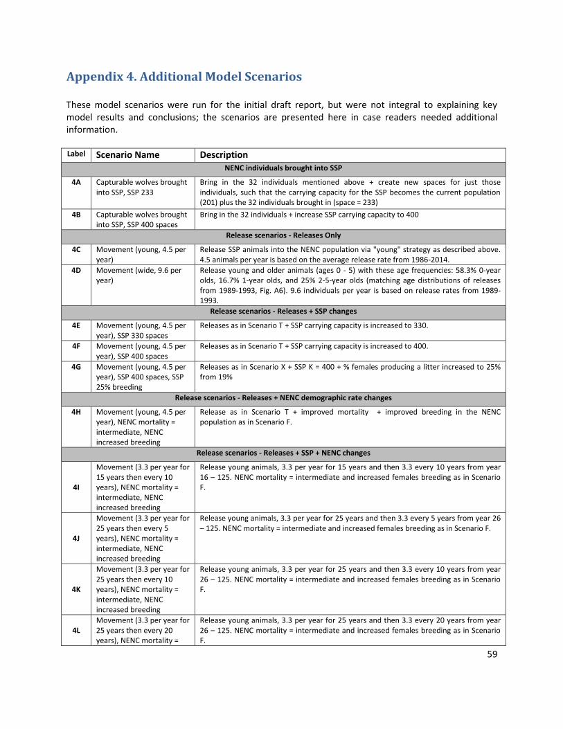
59

Appendix 4. Additional Model Scenarios These model scenarios were run for the initial draft report, but were not integral to explaining key model results and conclusions; the scenarios are presented here in case readers needed additional information. Label Scenario Name Description

NENC individuals brought into SSP

4A Capturable wolves brought into SSP, SSP 233

Bring in the 32 individuals mentioned above + create new spaces for just those individuals, such that the carrying capacity for the SSP becomes the current population (201) plus the 32 individuals brought in (space = 233)

4B Capturable wolves brought into SSP, SSP 400 spaces

Bring in the 32 individuals + increase SSP carrying capacity to 400

Release scenarios - Releases Only

4C Movement (young, 4.5 per year)

Release SSP animals into the NENC population via "young" strategy as described above. 4.5 animals per year is based on the average release rate from 1986-2014.

4D Movement (wide, 9.6 per year)

Release young and older animals (ages 0 - 5) with these age frequencies: 58.3% 0-year olds, 16.7% 1-year olds, and 25% 2-5-year olds (matching age distributions of releases from 1989-1993, Fig. A6). 9.6 individuals per year is based on release rates from 1989-1993.

Release scenarios - Releases + SSP changes

4E Movement (young, 4.5 per year), SSP 330 spaces

Releases as in Scenario T + SSP carrying capacity is increased to 330.

4F Movement (young, 4.5 per year), SSP 400 spaces

Releases as in Scenario T + SSP carrying capacity is increased to 400.

4G Movement (young, 4.5 per year), SSP 400 spaces, SSP 25% breeding

Releases as in Scenario X + SSP K = 400 + % females producing a litter increased to 25% from 19%

Release scenarios - Releases + NENC demographic rate changes

4H Movement (young, 4.5 per year), NENC mortality = intermediate, NENC increased breeding

Release as in Scenario T + improved mortality + improved breeding in the NENC population as in Scenario F.

Release scenarios - Releases + SSP + NENC changes

4I

Movement (3.3 per year for 15 years then every 10 years), NENC mortality = intermediate, NENC increased breeding

Release young animals, 3.3 per year for 15 years and then 3.3 every 10 years from year 16 – 125. NENC mortality = intermediate and increased females breeding as in Scenario F.

4J

Movement (3.3 per year for 25 years then every 5 years), NENC mortality = intermediate, NENC increased breeding

Release young animals, 3.3 per year for 25 years and then 3.3 every 5 years from year 26 – 125. NENC mortality = intermediate and increased females breeding as in Scenario F.

4K

Movement (3.3 per year for 25 years then every 10 years), NENC mortality = intermediate, NENC increased breeding

Release young animals, 3.3 per year for 25 years and then 3.3 every 10 years from year 26 – 125. NENC mortality = intermediate and increased females breeding as in Scenario F.

4L Movement (3.3 per year for 25 years then every 20 years), NENC mortality =

Release young animals, 3.3 per year for 25 years and then 3.3 every 20 years from year 26 – 125. NENC mortality = intermediate and increased females breeding as in Scenario F.

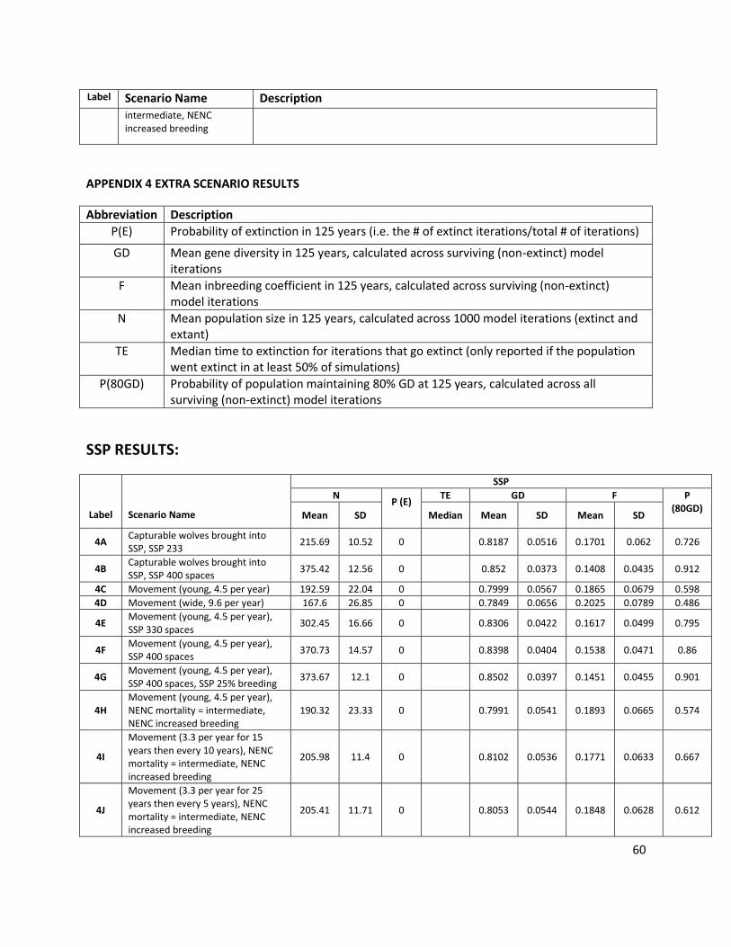
60

Label Scenario Name Description intermediate, NENC increased breeding

APPENDIX 4 EXTRA SCENARIO RESULTS

Abbreviation Description

P(E) Probability of extinction in 125 years (i.e. the # of extinct iterations/total # of iterations)

GD Mean gene diversity in 125 years, calculated across surviving (non-extinct) model iterations

F Mean inbreeding coefficient in 125 years, calculated across surviving (non-extinct) model iterations

N Mean population size in 125 years, calculated across 1000 model iterations (extinct and extant)

TE Median time to extinction for iterations that go extinct (only reported if the population went extinct in at least 50% of simulations)

P(80GD) Probability of population maintaining 80% GD at 125 years, calculated across all surviving (non-extinct) model iterations

SSP RESULTS:

Label

Scenario Name

SSP

N P (E)

TE GD F P (80GD)

Mean SD Median Mean SD Mean SD

4A Capturable wolves brought into SSP, SSP 233

215.69 10.52 0 0.8187 0.0516 0.1701 0.062 0.726

4B Capturable wolves brought into SSP, SSP 400 spaces

375.42 12.56 0 0.852 0.0373 0.1408 0.0435 0.912

4C Movement (young, 4.5 per year) 192.59 22.04 0 0.7999 0.0567 0.1865 0.0679 0.598

4D Movement (wide, 9.6 per year) 167.6 26.85 0 0.7849 0.0656 0.2025 0.0789 0.486

4E Movement (young, 4.5 per year), SSP 330 spaces

302.45 16.66 0 0.8306 0.0422 0.1617 0.0499 0.795

4F Movement (young, 4.5 per year), SSP 400 spaces

370.73 14.57 0 0.8398 0.0404 0.1538 0.0471 0.86

4G Movement (young, 4.5 per year), SSP 400 spaces, SSP 25% breeding

373.67 12.1 0 0.8502 0.0397 0.1451 0.0455 0.901

4H Movement (young, 4.5 per year), NENC mortality = intermediate, NENC increased breeding

190.32 23.33 0 0.7991 0.0541 0.1893 0.0665 0.574

4I

Movement (3.3 per year for 15 years then every 10 years), NENC mortality = intermediate, NENC increased breeding

205.98 11.4 0 0.8102 0.0536 0.1771 0.0633 0.667

4J

Movement (3.3 per year for 25 years then every 5 years), NENC mortality = intermediate, NENC increased breeding

205.41 11.71 0 0.8053 0.0544 0.1848 0.0628 0.612

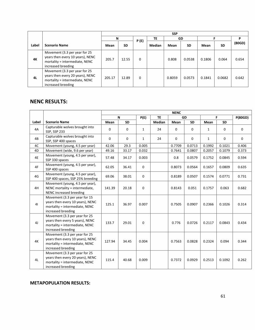
61

Label

Scenario Name

SSP

N P (E)

TE GD F P (80GD)

Mean SD Median Mean SD Mean SD

4K

Movement (3.3 per year for 25 years then every 10 years), NENC mortality = intermediate, NENC increased breeding

205.7 12.55 0 0.808 0.0538 0.1806 0.064 0.654

4L

Movement (3.3 per year for 25 years then every 20 years), NENC mortality = intermediate, NENC increased breeding

205.17 12.89 0 0.8059 0.0573 0.1841 0.0682 0.642

NENC RESULTS:

Label

Scenario Name

NENC

N P(E)

TE GD F P(80GD) Mean SD Median Mean SD Mean SD

4A Capturable wolves brought into SSP, SSP 233

0 0 1 24 0 0 1 0 0

4B Capturable wolves brought into SSP, SSP 400 spaces

0 0 1 24 0 0 1 0 0

4C Movement (young, 4.5 per year) 42.06 29.3 0.005 0.7709 0.0713 0.1992 0.1021 0.406

4D Movement (wide, 9.6 per year) 49.16 33.17 0.032 0.7641 0.0807 0.2057 0.1079 0.373

4E Movement (young, 4.5 per year), SSP 330 spaces

57.48 34.17 0.003 0.8 0.0579 0.1752 0.0845 0.594

4F Movement (young, 4.5 per year), SSP 400 spaces

62.05 36.41 0 0.8073 0.0564 0.1657 0.0809 0.635

4G Movement (young, 4.5 per year), SSP 400 spaces, SSP 25% breeding

69.06 38.01 0 0.8189 0.0507 0.1574 0.0771 0.731

4H Movement (young, 4.5 per year), NENC mortality = intermediate, NENC increased breeding

141.39 20.18 0 0.8143 0.051 0.1757 0.063 0.682

4I

Movement (3.3 per year for 15 years then every 10 years), NENC mortality = intermediate, NENC increased breeding

125.1 36.97 0.007 0.7505 0.0907 0.2366 0.1026 0.314

4J

Movement (3.3 per year for 25 years then every 5 years), NENC mortality = intermediate, NENC increased breeding

133.7 29.01 0 0.776 0.0726 0.2117 0.0843 0.434

4K

Movement (3.3 per year for 25 years then every 10 years), NENC mortality = intermediate, NENC increased breeding

127.94 34.45 0.004 0.7563 0.0828 0.2324 0.094 0.344

4L

Movement (3.3 per year for 25 years then every 20 years), NENC mortality = intermediate, NENC increased breeding

115.4 40.68 0.009 0.7372 0.0929 0.2513 0.1092 0.262

METAPOPULATION RESULTS:

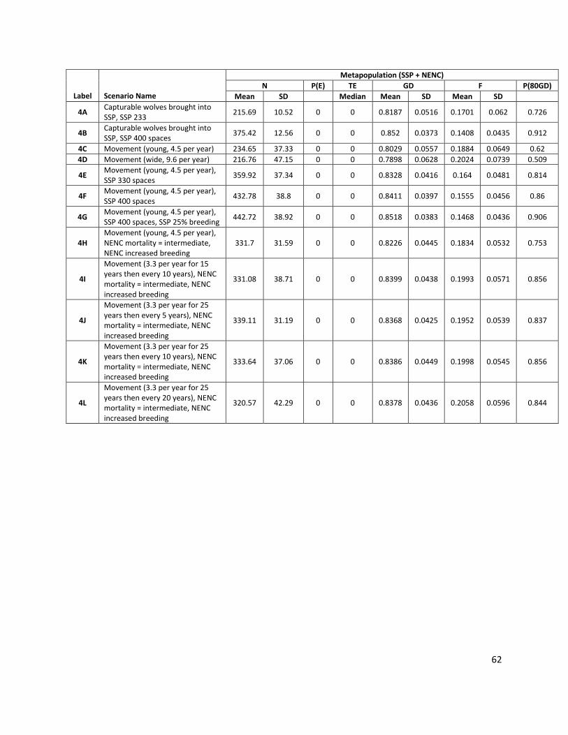
62

Label

Scenario Name

Metapopulation (SSP + NENC)

N P(E) TE GD F P(80GD)

Mean SD

Median Mean SD Mean SD

4A Capturable wolves brought into SSP, SSP 233

215.69 10.52 0 0 0.8187 0.0516 0.1701 0.062 0.726

4B Capturable wolves brought into SSP, SSP 400 spaces

375.42 12.56 0 0 0.852 0.0373 0.1408 0.0435 0.912

4C Movement (young, 4.5 per year) 234.65 37.33 0 0 0.8029 0.0557 0.1884 0.0649 0.62

4D Movement (wide, 9.6 per year) 216.76 47.15 0 0 0.7898 0.0628 0.2024 0.0739 0.509

4E Movement (young, 4.5 per year), SSP 330 spaces

359.92 37.34 0 0 0.8328 0.0416 0.164 0.0481 0.814

4F Movement (young, 4.5 per year), SSP 400 spaces

432.78 38.8 0 0 0.8411 0.0397 0.1555 0.0456 0.86

4G Movement (young, 4.5 per year), SSP 400 spaces, SSP 25% breeding

442.72 38.92 0 0 0.8518 0.0383 0.1468 0.0436 0.906

4H Movement (young, 4.5 per year), NENC mortality = intermediate, NENC increased breeding

331.7 31.59 0 0 0.8226 0.0445 0.1834 0.0532 0.753

4I

Movement (3.3 per year for 15 years then every 10 years), NENC mortality = intermediate, NENC increased breeding

331.08 38.71 0 0 0.8399 0.0438 0.1993 0.0571 0.856

4J

Movement (3.3 per year for 25 years then every 5 years), NENC mortality = intermediate, NENC increased breeding

339.11 31.19 0 0 0.8368 0.0425 0.1952 0.0539 0.837

4K

Movement (3.3 per year for 25 years then every 10 years), NENC mortality = intermediate, NENC increased breeding

333.64 37.06 0 0 0.8386 0.0449 0.1998 0.0545 0.856

4L

Movement (3.3 per year for 25 years then every 20 years), NENC mortality = intermediate, NENC increased breeding

320.57 42.29 0 0 0.8378 0.0436 0.2058 0.0596 0.844