Recursive Merge-Filter Algorithm for Computing the Discrete Wavelet Transform

Kunal Mukherjee and Amar Mukherjee

Abstract We present a new wavelet transform algorithm with a data flow that can fully exploit the

locality property of wavelets. This leads to highly optimized fine grained wavelet coding algo-

rithms, in terms of pipelining performance, flexible data granularity and reliability of transmis-

sion. It can be used by all wavelet coding methods, and has been demonstrated to improve the

performance of the most successful ones. We propose a new bottom-up Embedded Zerotree

Wavelet (EZW) image coding algorithm, and demonstrate a 5-10% speedup over EZW, by means

of close coupling between the new wavelet transform algorithm and the EZW encoding. The

Recursive Merge Filter (RMF) operator introduced in this paper reduces the complexity of creat-

ing larger DWTs of size 2N, from smaller ones of size N, by O(logN). Because this is a frequent

operation in the training process of the wavelet based hierarchical vector quantization (W-HVQ)

method, the result is a significant speedup overall. The RMF algorithm facilitates new fine

grained wavelet codecs, based on EZW encoding of sub-images using our new bottom-up algo-

rithm - this can give rise to future standards along the lines of “wavelet JPEG” and “wavelet

MPEG”.

Keywords: recursive merge filter, wavelet transform, hierarchical vector quantization,

zero tree

1

1.0 Introduction

In current wavelet-based codecs (e.g. [1], [3], [8]) the discrete wavelet transform (DWT)

is treated as a “black box” which cannot start generating the code until the entire image has been

transformed. This gives rise to several limitations, such as:

• performance - the computations in these codecs cannot be pipelined until after the entire trans-

form is computed;

• functionality - it is impossible to generate code at the sub-image level, i.e. fine-grained coding

is not possible; and

• reliability - monolithic code, i.e code for the entire image is more susceptible to channel errors

than fine grained code at the sub-image level, e.g. DCT-based codecs like JPEG and MPEG.

The contribution of this paper is a new wavelet transform algorithm developed specifi-

cally for wavelet-based image and video coding, called the Recursive Merge Filter (RMF) algo-

rithm. The data flow of this algorithm exploits the “locality” property of wavelets (e.g. see [7]) to

ensure that intermediate results can be used in the sense of complete DWTs of sub-images of the

input image. Stronger coupling and pipelining between the transform and the coding stages is

made possible because the wavelet transform of the entire image is constructed in a bottom-up

fashion, by merging smaller DWTs into larger ones. Thus, encoding algorithms, multi-resolution

compression, browsing applications etc. can now efficiently access and use the intermediate

stages of the transform.

The data flow of the RMF wavelet transform algorithm exploits the property of spatial

coherence (i.e. intermediate sub-arrays of DWT coefficients occupy the same positions as the

original data). This property leads to a speedup of existing algorithms like EZW [3] and SPIHT

[8], and also gives rise to new wavelet coding algorithms with flexible data granularity. We also

2

introduce the property of constant time “DWT growing”, or combining smaller DWTs into larger

ones. This is shown to result in significant speedup of certain compression algorithms like wave-

let based hierarchical vector quantization (W-HVQ) [2].

The organization of this paper is as follows. In Section 2 we will introduce the Fast Wave-

let Transform (FWT) paradigm for computing the DWT, and the limitations that it imposes on

image coding. In Section 3, we give a formal, recursive notation to describe the RMF operator,

and describe the DWT algorithm in terms of this operator. Next we prove correctness and algo-

rithmic efficiency by showing that the RMF and FWT algorithms are equivalent both in terms of

complexity and input/output behavior. We then proceed to give other properties of the RMF, and

generalize the algorithm to 2-D (two dimensions) and higher dimensions. We also generalize it to

work with arbitrary separable wavelet filters [7], and discuss the broader implications of the RMF

data flow on wavelet image coding.

In Section 4 we present the impact of the RMF paradigm in the application area of image

compression. We highlight the increased efficiency that RMF brings to the W-HVQ training pro-

cedure [1], [2], the tight coupling that is now possible between the DWT computing and the EZW

code generation processes, and the creation of new wavelet-based block codecs based on EZW-

coded wavelet transforms instead of Huffman-coded DCT, e.g. JPEG, MPEG [16].

In Section 5 we give experimental results, and close in Section 6 with a discussion of

future work and open research problems in this domain.

2.0 Fast Wavelet Transform Algorithm

The DWT can be described as a multi-resolution decomposition of a sequence (see [5]).

The DWT can be formally described using the Pyramid Algorithm (PA) notation (see [11]) as:

3

(1)

(2)

The PA takes a sequence (or signal), x(n), of length N as input, and generates a sequence

of length N as output. The output has N/2 values at the highest resolution, N/4 values at the next

resolution, and so on. Let N=2J, and let the number of frequency bands, or resolutions be J, i.e. we

are considering J=logN such bands or octaves, and the frequency index, j, varies in the range: 1..

J, corresponding to the range of frequency resolutions: 21, 22,..., 2J. WL and WH stand for the low-

pass and high-pass coefficient arrays respectively; n = 1,2,..., 2J-j; WL(0, n) = x(n) (i.e. the initial

array of data to be transformed); h(m) and g(m) are the quadrature mirror filters (QMFs) derived

from the wavelet; and L is the length of h and g (also called the number of taps of these filters).

The final output of the DWT will eventually be contained in WH, the first row containing N/2 out-

puts, the second row containing N/4 outputs, and so on.

2.1 Data flow of the Fast Wavelet Transform

In the Fast Wavelet Transform (FWT), the DWT computation proceeds through a succes-

sion of (filter, permute) operations, halving the effective vector (and filter) size after each such

operation, and permuting the newly computed “detail” coefficients to the bottom half of the old

WL j n,( ) WL j 1 2n m–,–( )h m( )

m 0=

L 1–

∑=

WH j n,( ) WL j 1 2n m–,–( )g m( )

m 0=

L 1–

∑=

4

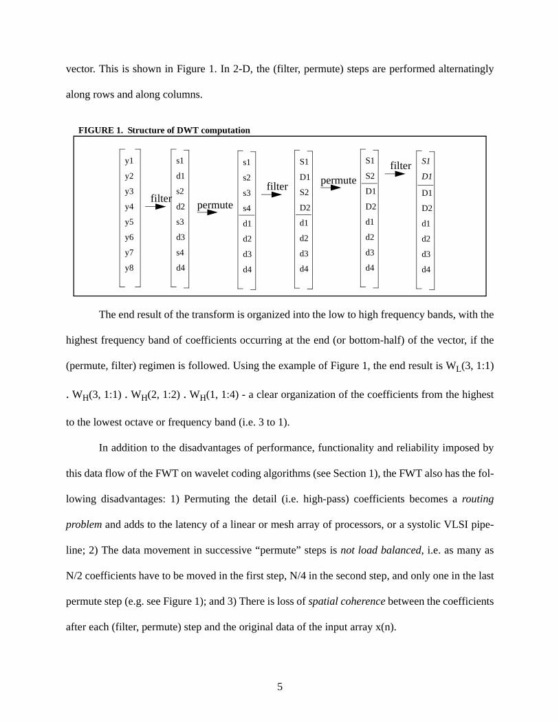
vector. This is shown in Figure 1. In 2-D, the (filter, permute) steps are performed alternatingly

along rows and along columns.

FIGURE 1. Structure of DWT computation

The end result of the transform is organized into the low to high frequency bands, with the

highest frequency band of coefficients occurring at the end (or bottom-half) of the vector, if the

(permute, filter) regimen is followed. Using the example of Figure 1, the end result is WL(3, 1:1)

. WH(3, 1:1) . WH(2, 1:2) . WH(1, 1:4) - a clear organization of the coefficients from the highest

to the lowest octave or frequency band (i.e. 3 to 1).

In addition to the disadvantages of performance, functionality and reliability imposed by

this data flow of the FWT on wavelet coding algorithms (see Section 1), the FWT also has the fol-

lowing disadvantages: 1) Permuting the detail (i.e. high-pass) coefficients becomes a routing

problem and adds to the latency of a linear or mesh array of processors, or a systolic VLSI pipe-

line; 2) The data movement in successive “permute” steps is not load balanced, i.e. as many as

N/2 coefficients have to be moved in the first step, N/4 in the second step, and only one in the last

permute step (e.g. see Figure 1); and 3) There is loss of spatial coherence between the coefficients

after each (filter, permute) step and the original data of the input array x(n).

y1

y2

filtery3

y4

y5

y6

y7

y8

permute

s1

d1

s2

d2

s3

d3

s4

d4

s1

s2

s3

s4

d1

d2

d3

d4

filterS1

D1

S2

D2

d1

d2

d3

d4

permute

S1

S2

D1

D2

d1

d2

d3

d4

S1

D1

D1

D2

d1

d2

d3

d4

filter

5

We will explain spatial coherence with reference to Figure 1. After the first filter step, the

coefficients (s1, d1) comprise the complete DWT of the sub-array (x1, x2). Similarly, (s2, d2) cor-

respond to the DWT of the sub-array (x3, x4), and so on. At this point, the array contains four

complete DWTs of sub-arrays of length two, and these DWTs occupy the same positions of the

array as the original sub-arrays, e.g. (s1, d1) occupy the same positions as (x1, x2), and so on. We

call this the spatial coherence property. In Figure 1, it is easy to see that the next operation, i.e. the

“permute” step shuffles the smooth and difference coefficients, thus destroying the spatial coher-

ence. As we shall shown in future sections, spatial coherence can be a very useful property, if a

wavelet coding algorithm can use the intermediate results of the transform, by interpreting them

as complete DWTs of sub-arrays of the original array.

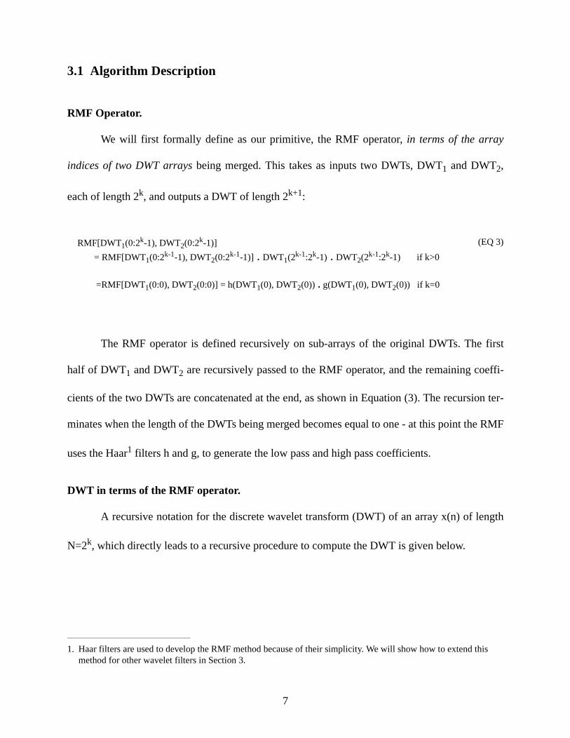
3.0 The Recursive Merge Filter Algorithm

In this section we will describe the Recursive Merge Filter (RMF) algorithm to compute

the DWT, prove correctness, generalize it to work with arbitrary separable wavelet filters and to

higher dimensions. We also discuss the implications of this algorithm on image compression. The

RMF algorithm computes the DWT of an array of length N in a bottom-up fashion, by succes-

sively “merging” two smaller DWTs (four in 2-D), and applying the wavelet filter to only the

“smooth” or DC coefficients.

6

3.1 Algorithm Description

RMF Operator.

We will first formally define as our primitive, the RMF operator, in terms of the array

indices of two DWT arrays being merged. This takes as inputs two DWTs, DWT1 and DWT2,

each of length 2k, and outputs a DWT of length 2k+1:

(EQ 3)

The RMF operator is defined recursively on sub-arrays of the original DWTs. The first

half of DWT1 and DWT2 are recursively passed to the RMF operator, and the remaining coeffi-

cients of the two DWTs are concatenated at the end, as shown in Equation (3). The recursion ter-

minates when the length of the DWTs being merged becomes equal to one - at this point the RMF

uses the Haar1 filters h and g, to generate the low pass and high pass coefficients.

DWT in terms of the RMF operator.

A recursive notation for the discrete wavelet transform (DWT) of an array x(n) of length

N=2k, which directly leads to a recursive procedure to compute the DWT is given below.

1. Haar filters are used to develop the RMF method because of their simplicity. We will show how to extend this method for other wavelet filters in Section 3.

RMF[DWT1(0:2k-1), DWT2(0:2k-1)]

= RMF[DWT1(0:2k-1-1), DWT2(0:2k-1-1)] . DWT1(2k-1:2k-1) . DWT2(2k-1:2k-1) if k>0

=RMF[DWT1(0:0), DWT2(0:0)] = h(DWT1(0), DWT2(0)) . g(DWT1(0), DWT2(0)) if k=0

7

(4)

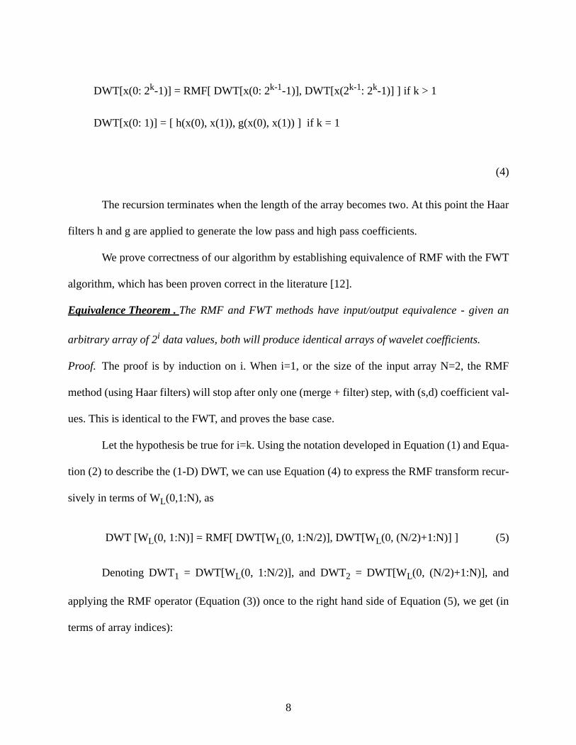
The recursion terminates when the length of the array becomes two. At this point the Haar

filters h and g are applied to generate the low pass and high pass coefficients.

We prove correctness of our algorithm by establishing equivalence of RMF with the FWT

algorithm, which has been proven correct in the literature [12].

Equivalence Theorem . The RMF and FWT methods have input/output equivalence - given an

arbitrary array of 2i data values, both will produce identical arrays of wavelet coefficients.

Proof. The proof is by induction on i. When i=1, or the size of the input array N=2, the RMF

method (using Haar filters) will stop after only one (merge + filter) step, with (s,d) coefficient val-

ues. This is identical to the FWT, and proves the base case.

Let the hypothesis be true for i=k. Using the notation developed in Equation (1) and Equa-

tion (2) to describe the (1-D) DWT, we can use Equation (4) to express the RMF transform recur-

sively in terms of WL(0,1:N), as

DWT [WL(0, 1:N)] = RMF[ DWT[WL(0, 1:N/2)], DWT[WL(0, (N/2)+1:N)] ] (5)

Denoting DWT1 = DWT[WL(0, 1:N/2)], and DWT2 = DWT[WL(0, (N/2)+1:N)], and

applying the RMF operator (Equation (3)) once to the right hand side of Equation (5), we get (in

terms of array indices):

DWT[x(0: 2k-1)] = RMF[ DWT[x(0: 2k-1-1)], DWT[x(2k-1: 2k-1)] ] if k > 1

DWT[x(0: 1)] = [ h(x(0), x(1)), g(x(0), x(1)) ] if k = 1

8

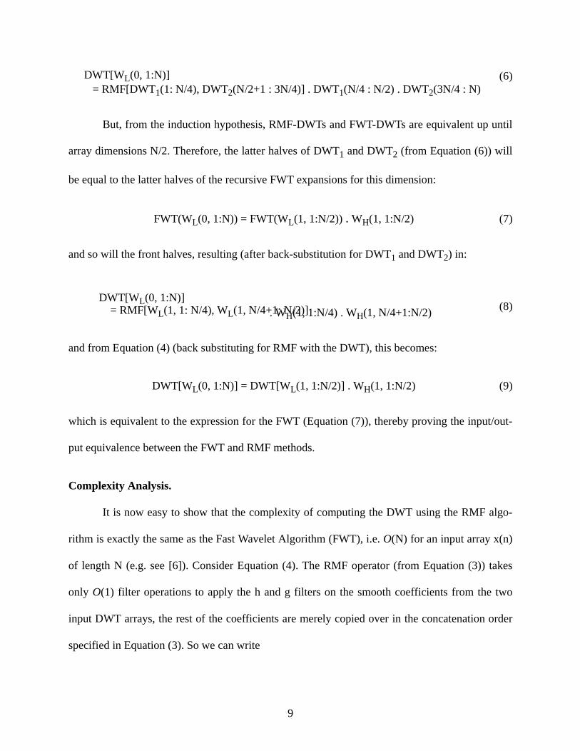
(6)

But, from the induction hypothesis, RMF-DWTs and FWT-DWTs are equivalent up until

array dimensions N/2. Therefore, the latter halves of DWT1 and DWT2 (from Equation (6)) will

be equal to the latter halves of the recursive FWT expansions for this dimension:

FWT(WL(0, 1:N)) = FWT(WL(1, 1:N/2)) . WH(1, 1:N/2) (7)

and so will the front halves, resulting (after back-substitution for DWT1 and DWT2) in:

(8)

and from Equation (4) (back substituting for RMF with the DWT), this becomes:

DWT[WL(0, 1:N)] = DWT[WL(1, 1:N/2)] . WH(1, 1:N/2) (9)

which is equivalent to the expression for the FWT (Equation (7)), thereby proving the input/out-

put equivalence between the FWT and RMF methods.

Complexity Analysis.

It is now easy to show that the complexity of computing the DWT using the RMF algo-

rithm is exactly the same as the Fast Wavelet Algorithm (FWT), i.e. O(N) for an input array x(n)

of length N (e.g. see [6]). Consider Equation (4). The RMF operator (from Equation (3)) takes

only O(1) filter operations to apply the h and g filters on the smooth coefficients from the two

input DWT arrays, the rest of the coefficients are merely copied over in the concatenation order

specified in Equation (3). So we can write

DWT[WL(0, 1:N)] = RMF[DWT1(1: N/4), DWT2(N/2+1 : 3N/4)] . DWT1(N/4 : N/2) . DWT2(3N/4 : N)

DWT[WL(0, 1:N)] . WH(1, 1:N/4) . WH(1, N/4+1:N/2) = RMF[WL(1, 1: N/4), WL(1, N/4+1: N/2)]

9

T(N) = 2T(N/2) + O(1) = O(N) (10)

where T(N) denotes the complexity of computing the RMF transform for input of size N.

3.2 Other Theoretical Properties of the RMF algorithm

In this section, we prove three other important properties of the RMF algorithm.

Invariant Theorem. The following invariant property holds during k successive (merge, filter)

stages of the RMF: after the ith stage, the intermediate (wavelet) coefficients occur as N/2i com-

plete DWTs of successive sub-arrays of the original data array, each sub-array being of length 2i.

This property is obvious from Equation (4), which enforces spatial ordering recursively,

due to the concatenation rule in Equation (4).

Corollary 1: Spatial Coherence Property. After the ith (merge + filter) step of the RMF, the N/2i

complete DWTs occupy exactly those positions of the array, as were occupied by the original data

elements which correspond to their inverse DWT.

This is directly a consequence of the Invariant Theorem, and the fact that there is no fur-

ther migration of coefficients beyond the limits of the two smaller sub-arrays which are merged at

the ith step.

It is difficult to maintain this kind of spatial coherence between input data and transform

coefficients in the Fourier or DCT transform domains, without introducing a significant amount

of positional side-information. This is because Fourier and DCTs don’t have the property of

“localization” like wavelet transforms [7].

Cheap DWT “growing” property. The complexity of combining two arbitrary, complete DWTs,

each of length 2i-1 into a complete DWT of length 2i takes a constant number of filter operations.

10

This is a consequence of the equivalence theorem, and the fact that one merge and filter

step of the RMF only uses the smooth coefficients from the two DWT arrays being merged. Thus,

the complexity of the “filter” part of a RMF operation is independent of the sizes of the coeffi-

cient arrays being merged, and is always equal to one each of h and g.

3.3 Generalization

To be widely applicable to image compression, we need to generalize the new algorithm to

work with different wavelet filters and in higher dimensions than one.

Wavelet Filters.

So far we have developed the RMF only with respect to the Haar wavelets, for simplicity. It is

possible to generalize it for arbitrary quadrature mirror filters (QMFs), h and g, of sizes (length, or

number of taps) htap and gtap respectively, as shown in Equation (11).

11

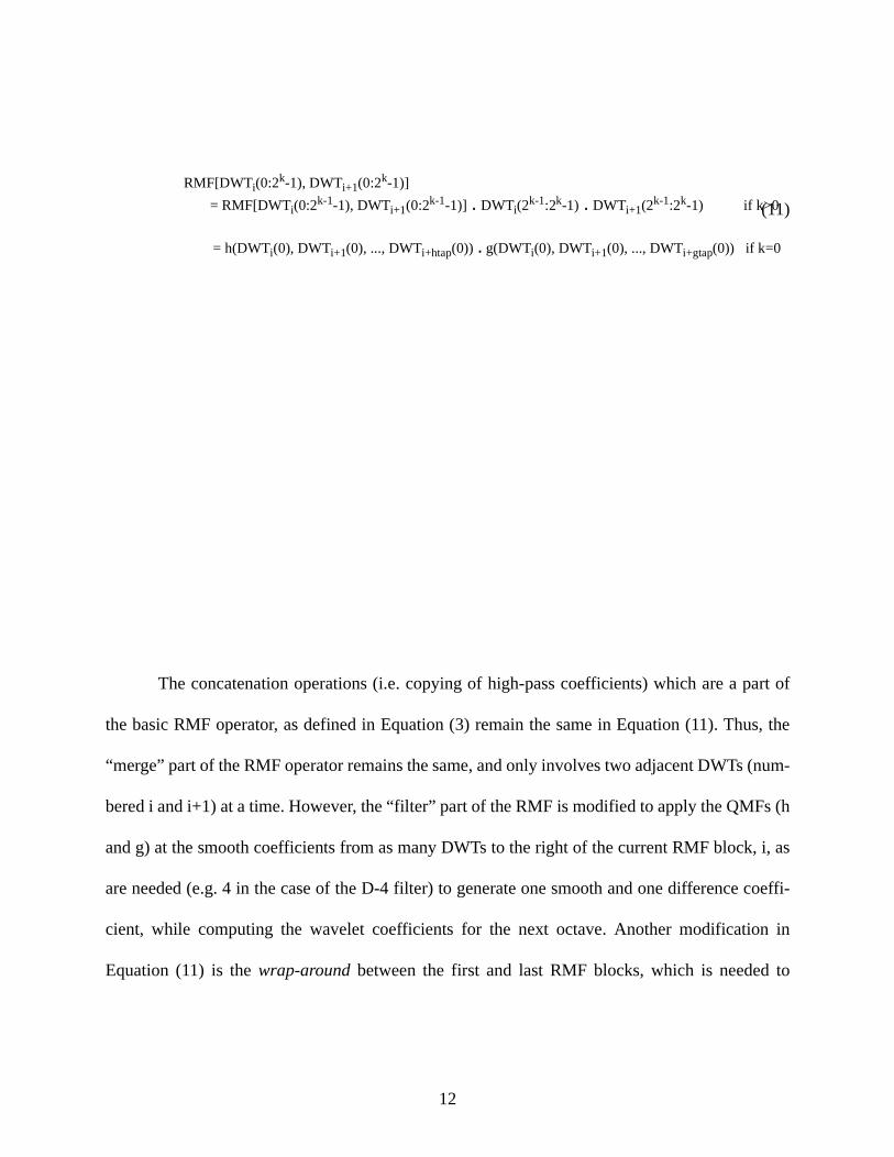
(11)

The concatenation operations (i.e. copying of high-pass coefficients) which are a part of

the basic RMF operator, as defined in Equation (3) remain the same in Equation (11). Thus, the

“merge” part of the RMF operator remains the same, and only involves two adjacent DWTs (num-

bered i and i+1) at a time. However, the “filter” part of the RMF is modified to apply the QMFs (h

and g) at the smooth coefficients from as many DWTs to the right of the current RMF block, i, as

are needed (e.g. 4 in the case of the D-4 filter) to generate one smooth and one difference coeffi-

cient, while computing the wavelet coefficients for the next octave. Another modification in

Equation (11) is the wrap-around between the first and last RMF blocks, which is needed to

RMF[DWTi(0:2k-1), DWTi+1(0:2k-1)]

= RMF[DWTi(0:2k-1-1), DWTi+1(0:2k-1-1)] . DWTi(2k-1:2k-1) . DWTi+1(2k-1:2k-1) if k>0

= h(DWTi(0), DWTi+1(0), ..., DWTi+htap(0)) . g(DWTi(0), DWTi+1(0), ..., DWTi+gtap(0)) if k=0

12

implement QMFs of length greater than 2, due to the technique of using circular convolutions at

the array boundaries [12].

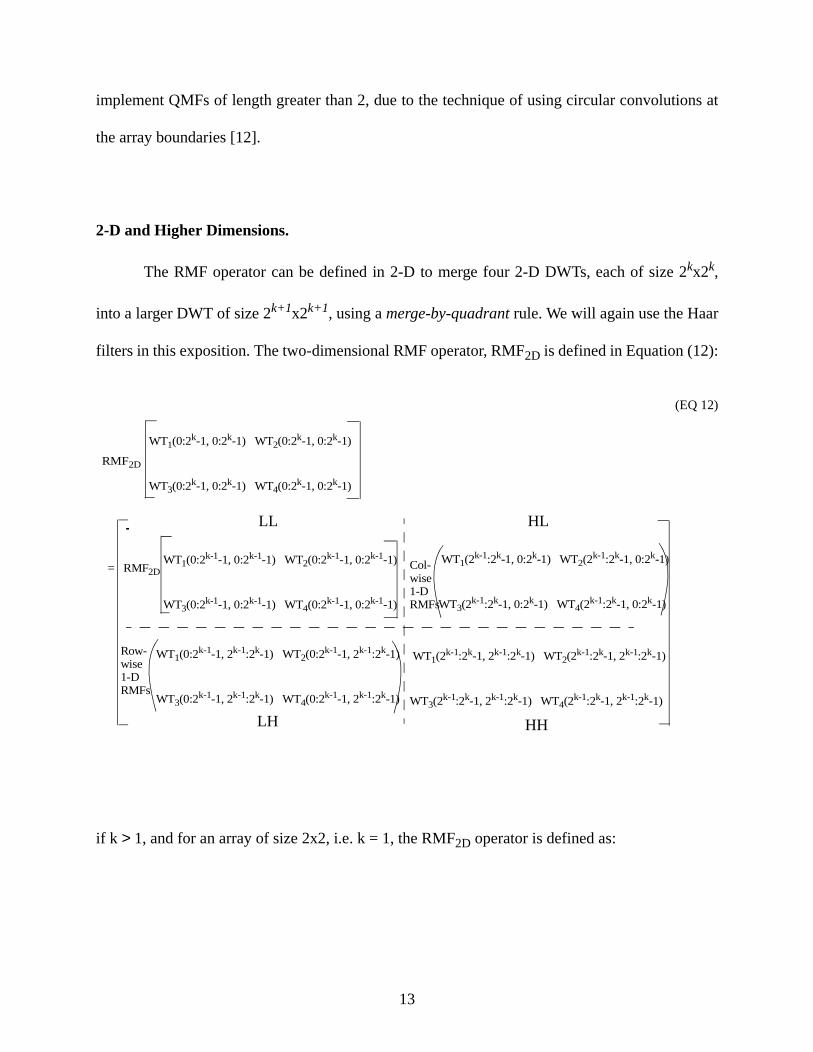
2-D and Higher Dimensions.

The RMF operator can be defined in 2-D to merge four 2-D DWTs, each of size 2kx2k,

into a larger DWT of size 2k+1x2k+1, using a merge-by-quadrant rule. We will again use the Haar

filters in this exposition. The two-dimensional RMF operator, RMF2D is defined in Equation (12):

(EQ 12)

if k > 1, and for an array of size 2x2, i.e. k = 1, the RMF2D operator is defined as:

WT1(0:2k-1, 0:2k-1) WT2(0:2k-1, 0:2k-1)

WT3(0:2k-1, 0:2k-1) WT4(0:2k-1, 0:2k-1)

= RMF2D WT1(0:2k-1-1, 0:2k-1-1) WT2(0:2k-1-1, 0:2k-1-1)

WT3(0:2k-1-1, 0:2k-1-1) WT4(0:2k-1-1, 0:2k-1-1)

WT1(2k-1:2k-1, 0:2k-1) WT2(2k-1:2k-1, 0:2k-1)

WT3(2k-1:2k-1, 0:2k-1) WT4(2k-1:2k-1, 0:2k-1)

WT1(0:2k-1-1, 2k-1:2k-1) WT2(0:2k-1-1, 2k-1:2k-1)

WT3(0:2k-1-1, 2k-1:2k-1) WT4(0:2k-1-1, 2k-1:2k-1)

WT1(2k-1:2k-1, 2k-1:2k-1) WT2(2k-1:2k-1, 2k-1:2k-1)

WT3(2k-1:2k-1, 2k-1:2k-1) WT4(2k-1:2k-1, 2k-1:2k-1)

RMF2D

Col-wise1-D

Row-wise1-D

RMFs

RMFs

LL HL

LH HH

13

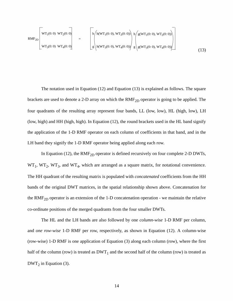
(13)

The notation used in Equation (12) and Equation (13) is explained as follows. The square

brackets are used to denote a 2-D array on which the RMF2D operator is going to be applied. The

four quadrants of the resulting array represent four bands, LL (low, low), HL (high, low), LH

(low, high) and HH (high, high). In Equation (12), the round brackets used in the HL band signify

the application of the 1-D RMF operator on each column of coefficients in that band, and in the

LH band they signify the 1-D RMF operator being applied along each row.

In Equation (12), the RMF2D operator is defined recursively on four complete 2-D DWTs,

WT1, WT2, WT3, and WT4, which are arranged as a square matrix, for notational convenience.

The HH quadrant of the resulting matrix is populated with concatenated coefficients from the HH

bands of the original DWT matrices, in the spatial relationship shown above. Concatenation for

the RMF2D operator is an extension of the 1-D concatenation operation - we maintain the relative

co-ordinate positions of the merged quadrants from the four smaller DWTs.

The HL and the LH bands are also followed by one column-wise 1-D RMF per column,

and one row-wise 1-D RMF per row, respectively, as shown in Equation (12). A column-wise

(row-wise) 1-D RMF is one application of Equation (3) along each column (row), where the first

half of the column (row) is treated as DWT1 and the second half of the column (row) is treated as

DWT2 in Equation (3).

RMF2D

WT1(0: 0) WT2(0: 0)

WT3(0: 0) WT4(0: 0)

=

h h(WT1(0: 0), WT2(0: 0))

g h(WT3(0: 0), WT4(0: 0))

h g(WT1(0: 0), WT2(0: 0))

g g(WT3(0: 0), WT4(0: 0))

14

The recursion of RMF2D continues only on the first quadrant of the matrix. The recursion

terminates when the size of each of the four DWTs being merged becomes 1x1 - at this point the

RMF2D acts as the Haar filters h and g, to generate the low pass and high pass coefficients, as

shown in Equation (13). This is exactly the same as the 2-D FWT algorithm acting on a 2x2 input

array (e.g. see [4]).

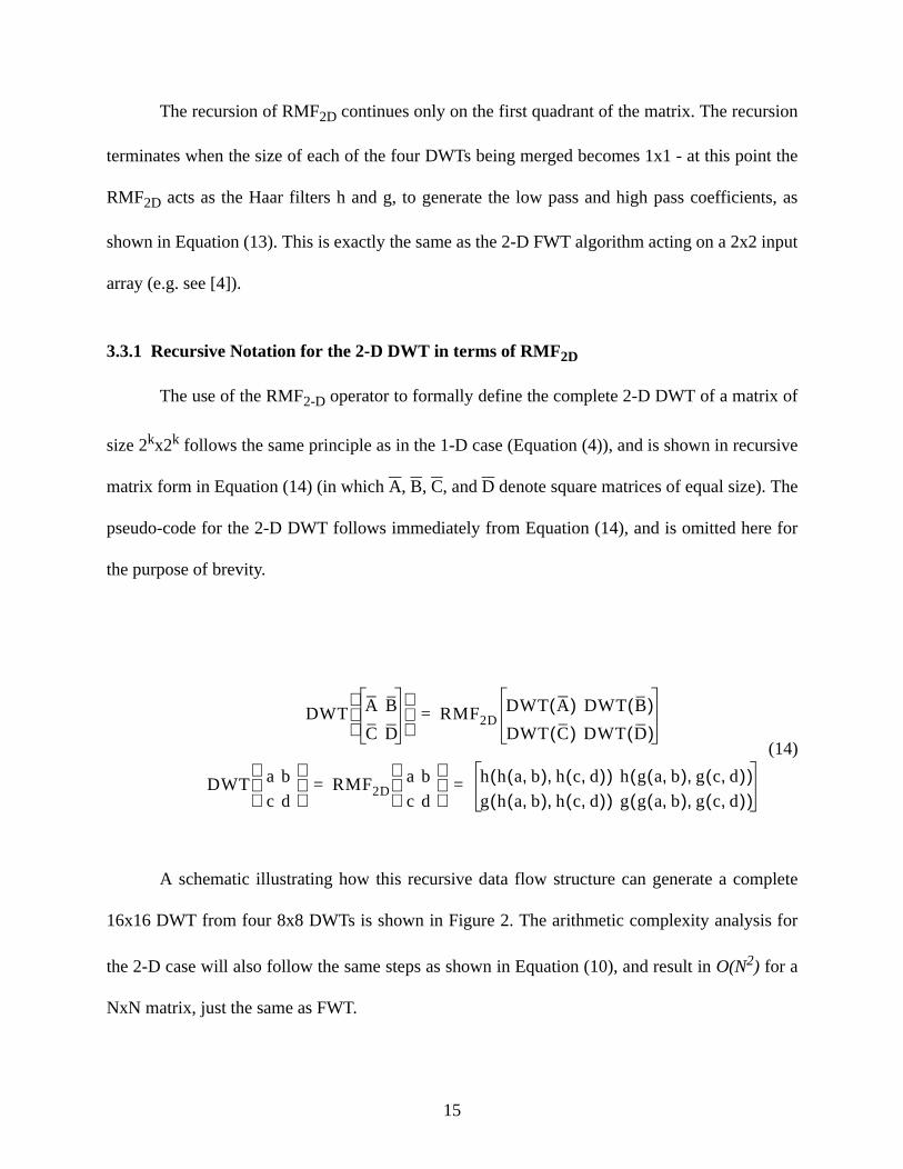
3.3.1 Recursive Notation for the 2-D DWT in terms of RMF2D

The use of the RMF2-D operator to formally define the complete 2-D DWT of a matrix of

size 2kx2k follows the same principle as in the 1-D case (Equation (4)), and is shown in recursive

matrix form in Equation (14) (in which A, B, C, and D denote square matrices of equal size). The

pseudo-code for the 2-D DWT follows immediately from Equation (14), and is omitted here for

the purpose of brevity.

(14)

A schematic illustrating how this recursive data flow structure can generate a complete

16x16 DWT from four 8x8 DWTs is shown in Figure 2. The arithmetic complexity analysis for

the 2-D case will also follow the same steps as shown in Equation (10), and result in O(N2) for a

NxN matrix, just the same as FWT.

DWT A B

C D

RMF2DDWT A( ) DWT B( )DWT C( ) DWT D( )

=

DWT a b

c d

RMF2Da b

c d h h a b,( ) h c d,( ),( ) h g a b,( ) g c d,( ),( )

g h a b,( ) h c d,( ),( ) g g a b,( ) g c d,( ),( )= =

15

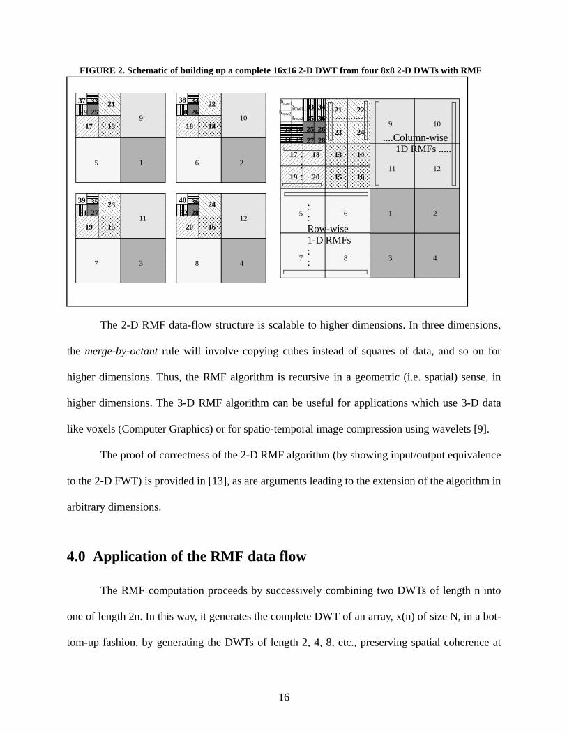
FIGURE 2. Schematic of building up a complete 16x16 2-D DWT from four 8x8 2-D DWTs with RMF

The 2-D RMF data-flow structure is scalable to higher dimensions. In three dimensions,

the merge-by-octant rule will involve copying cubes instead of squares of data, and so on for

higher dimensions. Thus, the RMF algorithm is recursive in a geometric (i.e. spatial) sense, in

higher dimensions. The 3-D RMF algorithm can be useful for applications which use 3-D data

like voxels (Computer Graphics) or for spatio-temporal image compression using wavelets [9].

The proof of correctness of the 2-D RMF algorithm (by showing input/output equivalence

to the 2-D FWT) is provided in [13], as are arguments leading to the extension of the algorithm in

arbitrary dimensions.

4.0 Application of the RMF data flow

The RMF computation proceeds by successively combining two DWTs of length n into

one of length 2n. In this way, it generates the complete DWT of an array, x(n) of size N, in a bot-

tom-up fashion, by generating the DWTs of length 2, 4, 8, etc., preserving spatial coherence at

1 2

3 4

5 6

7 8

9 10

11 12

13 14

15 16

17 18

19 20

21 22

23 24

25 26

27 28

29 30

31 32

33 34

35 36

37 38

39 40

43

215 6

7 8

9 10

11 121615

141317 18

19 20

21 22

23 2425 26

27 28

29 30

31 32

33 34

35 36

grow1

hrow1

grow2hrow2

....Column-wise 1D RMFs .....

::Row-wise1-D RMFs::

...........

:::

16

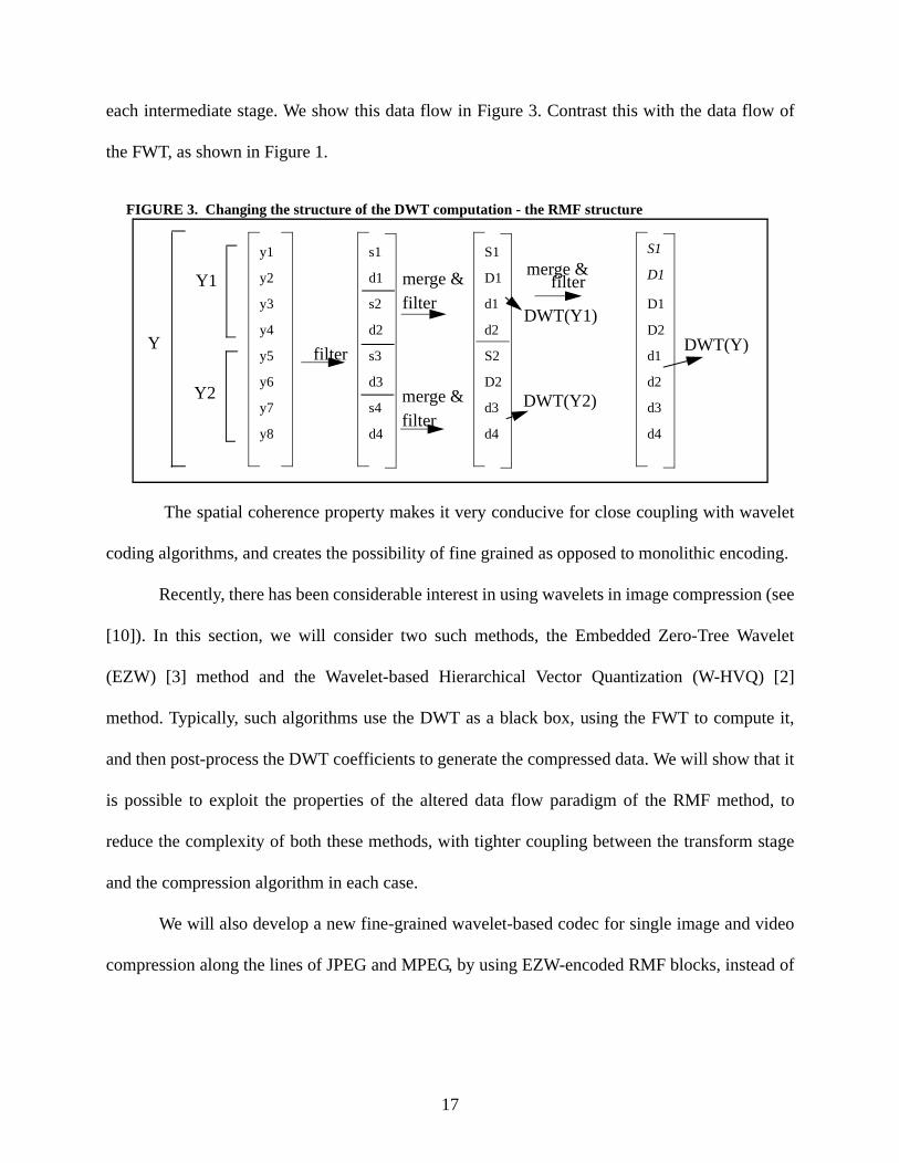
each intermediate stage. We show this data flow in Figure 3. Contrast this with the data flow of

the FWT, as shown in Figure 1.

FIGURE 3. Changing the structure of the DWT computation - the RMF structure

The spatial coherence property makes it very conducive for close coupling with wavelet

coding algorithms, and creates the possibility of fine grained as opposed to monolithic encoding.

Recently, there has been considerable interest in using wavelets in image compression (see

[10]). In this section, we will consider two such methods, the Embedded Zero-Tree Wavelet

(EZW) [3] method and the Wavelet-based Hierarchical Vector Quantization (W-HVQ) [2]

method. Typically, such algorithms use the DWT as a black box, using the FWT to compute it,

and then post-process the DWT coefficients to generate the compressed data. We will show that it

is possible to exploit the properties of the altered data flow paradigm of the RMF method, to

reduce the complexity of both these methods, with tighter coupling between the transform stage

and the compression algorithm in each case.

We will also develop a new fine-grained wavelet-based codec for single image and video

compression along the lines of JPEG and MPEG, by using EZW-encoded RMF blocks, instead of

y1

y2

filter

y3

y4

y5

y6

y7

y8

s1

d1

s2

d2

s3

d3

s4

d4

S1

D1

d1

d2

S2

D2

d3

d4

S1

D1

D1

D2

d1

d2

d3

d4

merge &filter

merge &filter

merge &filterY1

Y2 DWT(Y2)

DWT(Y1)

Y DWT(Y)

17

Huffman-encoded JPEG blocks, and provide several arguments as to why this should give an

improvement in performance.

4.1 Application of RMF in W-HVQ Training

The (merge, filter) operation suggests a way of combining two arbitrary DWTs into a

larger DWT, by simply applying O(1) filter applications (for each such operation) at the low-pass

coefficients from each of the smaller DWTs. We will exploit this property to significantly speed

up the W-HVQ training algorithm.

In the paper by Chaddha et. al. [2], block transforms (e.g. Haar, Walsh, etc.) of input vec-

tors of wavelet coefficients of size 2, 4, 8, etc. are stored in hierarchically constructed transform

tables during training. In the training phase, we create a 2-vector codebook, C2, of size N=28; a 4-

vector codebook, C4, of size N=28; a 8-vector codebook C8, of size N=28, and so on. Each of

these codebooks is indexed by two 8 bit numbers. First, each code vector in C2, C4, etc. is con-

structed by training on vectors of size 2x1, 2x2 etc. from the training set, using a standard training

algorithm like GLA [14]. During encoding, each successive stage of table-lookup implicitly per-

forms a 2:1 data compression and an incremental level of DWT, in cascaded fashion (e.g. see [1]).

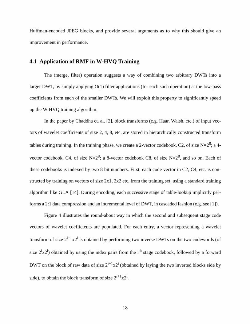
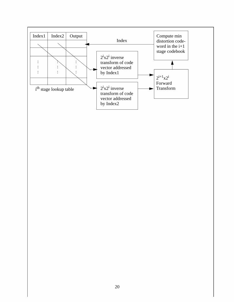
Figure 4 illustrates the round-about way in which the second and subsequent stage code

vectors of wavelet coefficients are populated. For each entry, a vector representing a wavelet

transform of size 2i+1x2i is obtained by performing two inverse DWTs on the two codewords (of

size 2ix2i) obtained by using the index pairs from the ith stage codebook, followed by a forward

DWT on the block of raw data of size 2i+1x2i (obtained by laying the two inverted blocks side by

side), to obtain the block transform of size 2i+1x2i.

18

19

Index1 Index2 Output

: : : : : : : : :

2ix2i inversetransform of code

2i+1x2i

ForwardTransform

Compute mindistortion code-word in the i+1stage codebook

Index

ith stage lookup table

vector addressedby Index1

2ix2i inversetransform of codevector addressedby Index2

20

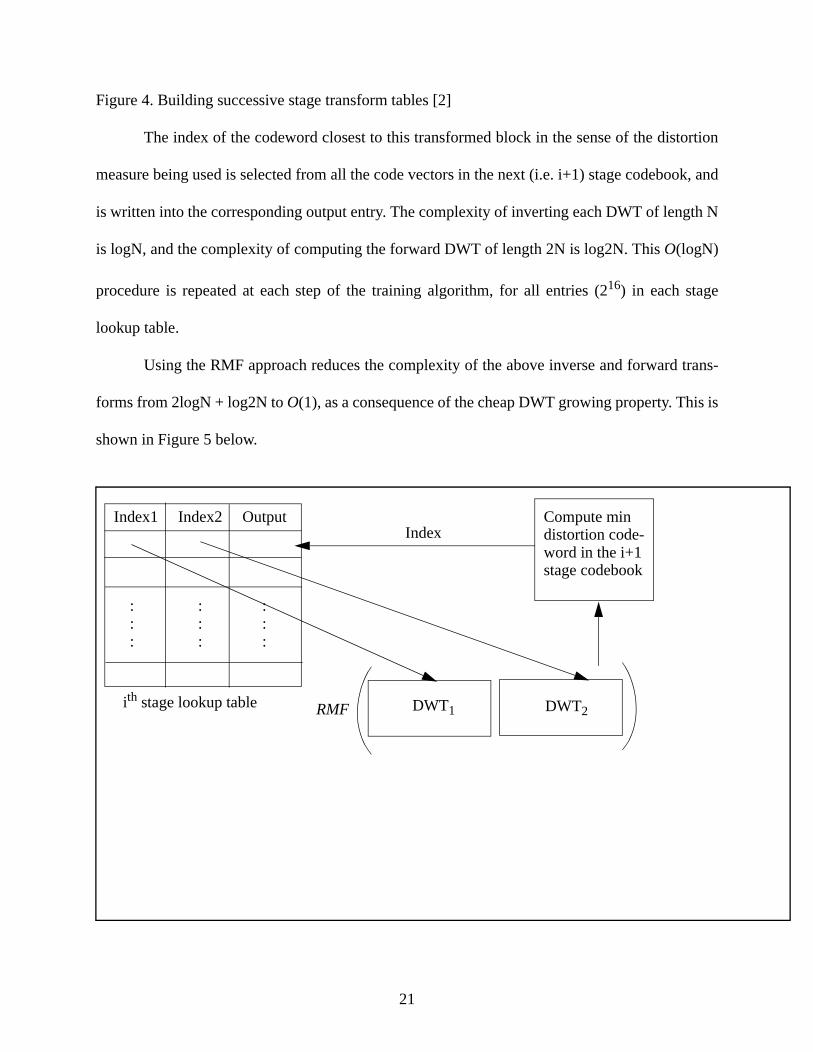
Figure 4. Building successive stage transform tables [2]

The index of the codeword closest to this transformed block in the sense of the distortion

measure being used is selected from all the code vectors in the next (i.e. i+1) stage codebook, and

is written into the corresponding output entry. The complexity of inverting each DWT of length N

is logN, and the complexity of computing the forward DWT of length 2N is log2N. This O(logN)

procedure is repeated at each step of the training algorithm, for all entries (216) in each stage

lookup table.

Using the RMF approach reduces the complexity of the above inverse and forward trans-

forms from 2logN + log2N to O(1), as a consequence of the cheap DWT growing property. This is

shown in Figure 5 below.

Index1 Index2 Output

: : : : : : : : :

Compute mindistortion code-word in the i+1stage codebook

Index

ith stage lookup table RMF DWT1 DWT2

21

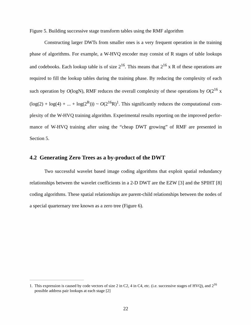
Figure 5. Building successive stage transform tables using the RMF algorithm

Constructing larger DWTs from smaller ones is a very frequent operation in the training

phase of algorithms. For example, a W-HVQ encoder may consist of R stages of table lookups

and codebooks. Each lookup table is of size 216. This means that 216 x R of these operations are

required to fill the lookup tables during the training phase. By reducing the complexity of each

such operation by O(logN), RMF reduces the overall complexity of these operations by O(216 x

(log(2) + log(4) + ... + log(2R))) ~ O(216R)1. This significantly reduces the computational com-

plexity of the W-HVQ training algorithm. Experimental results reporting on the improved perfor-

mance of W-HVQ training after using the “cheap DWT growing” of RMF are presented in

Section 5.

4.2 Generating Zero Trees as a by-product of the DWT

Two successful wavelet based image coding algorithms that exploit spatial redundancy

relationships between the wavelet coefficients in a 2-D DWT are the EZW [3] and the SPIHT [8]

coding algorithms. These spatial relationships are parent-child relationships between the nodes of

a special quarternary tree known as a zero tree (Figure 6).

1. This expression is caused by code vectors of size 2 in C2, 4 in C4, etc. (i.e. successive stages of HVQ), and 216 possible address pair lookups at each stage [2]

22

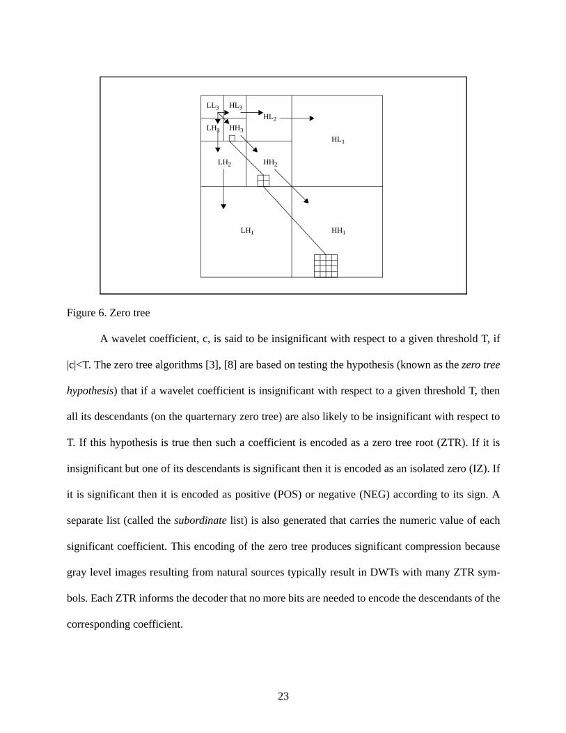
Figure 6. Zero tree

A wavelet coefficient, c, is said to be insignificant with respect to a given threshold T, if

|c|<T. The zero tree algorithms [3], [8] are based on testing the hypothesis (known as the zero tree

hypothesis) that if a wavelet coefficient is insignificant with respect to a given threshold T, then

all its descendants (on the quarternary zero tree) are also likely to be insignificant with respect to

T. If this hypothesis is true then such a coefficient is encoded as a zero tree root (ZTR). If it is

insignificant but one of its descendants is significant then it is encoded as an isolated zero (IZ). If

it is significant then it is encoded as positive (POS) or negative (NEG) according to its sign. A

separate list (called the subordinate list) is also generated that carries the numeric value of each

significant coefficient. This encoding of the zero tree produces significant compression because

gray level images resulting from natural sources typically result in DWTs with many ZTR sym-

bols. Each ZTR informs the decoder that no more bits are needed to encode the descendants of the

corresponding coefficient.

LL3 HL3

LH3 HH3

HL2

LH2 HH2

HL1

HH1LH1

23

The EZW algorithm [3] suffers from a fundamental performance drawback, because the

transform stage and the coding stage are completely decoupled. The zero tree scans (see [3]), i.e.

testing the zero tree hypothesis with respect to each threshold are not started until after the full 2-

D DWT has been computed. The RMF algorithm can speed up the EZW/SPIHT algorithms, by

allowing a tighter coupling between the DWT computing stage and the zero-tree finding stage, so

that the zero-tree can be generated as a by-product of the transform.

4.2.1 The Bottom-Up Zero Tree RMF Algorithm

The new algorithm simultaneously computes the 2-D DWT and the zero trees in bottom-

up fashion. At the ith stage, the complete DWTs of sub-images of size 2ix2i are computed by

applying the RMF2-D operator on the results of the previous (i-1th) step. Simultaneously, the max-

ima of absolute values in each band (HH, HL, LH) are also updated, to aid the zero tree computa-

tion. At any (e.g. ith) step, we may generate the zero tree codes of the sub-images. In this case, we

will not need to explore all the zero tree descendants as in [3]. Instead, we can deduce the code

symbols by using the band-wise maximum values that were propagated in bottom-up fashion.

The Bottom-up Zero Tree RMF algorithm consists of three main steps. Of these, only the

first two are applicable at each intermediate stage. The third step is only applied at the last RMF

step, to generate the zero tree code symbols, from the information generated in a bottom-up fash-

ion from the previous merge and filter steps. The pseudo-code for this algorithm is given in Figure

7. The algorithm is explained below, and is illustrated with an example. First we shall introduce

some basic terminology:

24

• The current_band_max of each band is the maximum absolute value of wavelet coefficients for

that band and its descendant bands, e.g. if 22 is the maximum absolute value in the bands HH2

and HH1, then band_max(HH2) = 22.

• The previous_band_max is the value that is propagated to the next step of the Zero-Tree RMF

algorithm, in order to efficiently generate the current_band_max values, thus propagating the

zero tree computations in a bottom-up fashion.

The band_max updates use the previous_band_max values from each of the four DWTs

participating in the RMF2D operation, and new values of current_band_max and wavelet coeffi-

cients that are generated in the current step of the RMF algorithm. The way in which the current

and previous band_max values are computed varies slightly for the HH, HL and LH bands.

In the new HHi band, current_band_max(HHi) is simply the maximum of the four

previous_band_max(HHi) values, and current_band_max (HHi-1). The current band_max is also

propagated to the next step of the RMF (in which four larger DWTs will be merged) as the

previous_band_max, i.e. previous_band_max(HHi) = current_band_max(HHi).

In the new HLi band, current_band_max(HLi) is the maximum of the four

previous_band_max(HLi) values, the new coefficients generated in the first two rows of the new

HLi by the column-wise 1-D RMF operations (see Equation (12)), and current_band_max(HLi-1).

The new value of the previous_band_max is the maximum of all the coefficients in the new HLi

band, except those in the first row. The reason for leaving out the values from the first row is that

these are the smooth coefficients, which will be replaced by the results of 1-D RMF filter applica-

tions in the next step of RMF2D.

25

Similarly, in the new LHi band, current_band_max(LHi) is the maximum of the four

previous_band_max(LHi) values, the new coefficients generated in the first two columns of the

new LHi by the row-wise 1-D RMF operations (Equation (12)), and current_band_max(LHi-1).

The new value of previous_band_max(LHi-1) is the maximum of all the coefficients in the new

HLi band, except those in the first column.

Step 1. The RMF2D operator is applied to construct a DWT of size 2i+1 x 2i+1 from four smaller

DWTs, each of size 2i x 2i, using Equation (12) and Equation (13).

Step 2. The current and previous values of band_max, i.e. current_band_max and

previous_band_max are updated for each band of the new (new signifies the larger DWT that is

being constructed from the four smaller DWTs) DWT.

Step 3. The third step is applied at the RMF step at which code is to be generated. This could be

the final step of the complete DWT, or an earlier stage if fine-grained (i.e. sub-image level) cod-

ing is being done (see Section 3.3.3). The zero tree symbols with respect to each threshold, T, are

generated for each node of the DWT in increasing order of octaves, i.e. octaves 1 through n, in the

following manner. If the absolute value of the coefficient is greater than T, then it is encoded as

POS or NEG (according to whether it is positive or negative). If it is insignificant, and the

band_max of the band containing its immediate children is also insignificant, then it is encoded

with the symbol 0. For example, for threshold T = 32, if a parent node in band HL2 has a value of

28 and band_max(HL1) = 24, then that node is encoded with 0. If the octave of the parent node is

also the highest octave in the DWT, or fine grained codes are to be generated at that octave, then

the symbol ZTR is used instead of 0. If the coefficient is insignificant, but the band_max of the

band containing its immediate children is significant, then we examine the code for each of its

26

four children. If they are all 0, then the coefficient is also encoded as 0 (or ZTR at the final octave

level). If they are not all 0, then the parent node is encoded with the IZ symbol.

The pseudo-code for the bottom up algorithm is given in Figure 7 below. WT1, WT2,

WT3 and WT4 are the four smaller DWTs that are inputs into the current step of the algorithm.

The notation WT1:WT4 denotes “from WT1, WT2, WT3 and WT4”.

4.2.2 A Simple Example

In this sub-section, a simple example will be used to highlight the order of operations in

the Bottom-Up Zero Tree RMF algorithm, with reference to Figure 8. In this step of the algo-

rithm, four DWTs of size 4x4 are merged and filtered, the band_max values are updated, and the

zero tree codes are generated for the threshold, T = 32. This example has been chosen such that

the end result is exactly the same as that obtained in an example worked out by Shapiro to illus-

trate the EZW algorithm [3], and by Rao and Bopardikar to illustrate the SPIHT algorithm [15].

Thus, for this example, we are able to verify input/output equivalence with these other two algo-

rithms that are also based on zero tree coding.

27

Figure 7. Bottom-up Zero Tree RMF algorithm working on four 2kx2k DWTs

WT1(0:2k-1, 0:2k-1) WT2(0:2k-1, 0:2k-1)

WT3(0:2k-1, 0:2k-1) WT4(0:2k-1, 0:2k-1)

RMF2D

ALGORITHM Bottom Up Zero Tree RMF (Inputs 2D_DWT: WT1, WT2, WT3, WT4){

for octave = 1 to k+1 do /* Step 2

/* Step 1 RMF2D */

current_band_max (HHoctave) = max (maxWT1:WT4( previous_band_max (HHoctave), current_band_max ( HHoctave-1)) previous_band_max (HHoctave) = current_band_max (HHoctave) current_band_max (HLoctave) = max (maxWT1:WT4( previous_band_max (HLoctave), max (1st two rows in HLoctave), current_band_max (HLoctave-1)) previous_band_max (HLoctave)

= max (maxWT1:WT4( previous_band_max (HLoctave), max ( second row in HLoctave)) current_band_max (LHoctave) = max (maxWT1:WT4( previous_band_max (LHoctave), max (1st two columns in LHoctave), current_band_max (LHoctave-1))

} endif done; else if all four children nodes are encoded 0 encode as 0, else encode as IZ

previous_band_max (LHoctave)

else if current_band_max(band of immediate children) is insignificant encode 0 if node is significant then if (node > 0) then encode POS else NEG

for ∀ THRESHOLDS and ∀ nodes in octaves 1 to k+1 do

if EZW coding at this level is required /* Step 3 Generate the Zero Tree codes */

= max (maxWT1:WT4( previous_band_max (LHoctave), max ( second column in LHoctave))done

Update current and previous band_max values */

28

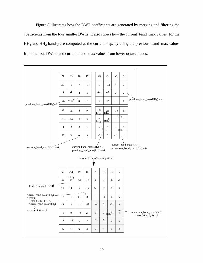
Figure 8 illustrates how the DWT coefficients are generated by merging and filtering the

coefficients from the four smaller DWTs. It also shows how the current_band_max values (for the

HH1 and HH2 bands) are computed at the current step, by using the previous_band_max values

from the four DWTs, and current_band_max values from lower octave bands.

21 63 10 17

29 3 5 -7

6 4 -1 4

3 -3 3 -2

43 -3 -6 6

1 -12 3 9

2 -2 47-14

3 2 0 4

37 35 4 9

-16 -14 4 -2

6 3 6 -1

16 5 0 3

151 23 -18 8

-2 8 3 2

6 3 -4 5

-6 6 -4 4

current_band_max(HH1)= previous_band_max(HH1) = 6

HH1

HL1

LH1

HL2

HH2LH2

LL2

current_band_max(LH1) = 6previous_band_max(LH1) = 6

63 -34 49 10

-31 23 14 -13

-12 3 14 15

-9 -7 -14 8

7 13 -12 7

3 4 6 -1

9 3 -7 5

4 -2 3 2

-5 9 -1 47

3 0 -3 2

-4 6 -3 2

5 11 5 6

4 6 -2 2

3 -2 0 4

6 3 6 3

0 3 -4 4

Bottom-Up Zero Tree Algorithm

previous_band_max(HH1) = 4

previous_band_max(HH1)=6

previous_band_max(HH1) = 6

current_band_max(HH1)= max ( 6, 4, 6, 6) = 6

HH1

HH2current_band_max(HH2)= max ( max (3, 12, 14, 8), current_band_max(HH1)

= max (14, 6) = 14 )

Code generated = ZTR

HH3

29

Figure 8. Example of the Bottom-up Zero Tree Algorithm (3-scale DWT)

The value of the HH3 coefficient generated by the RMF algorithm, 23, is insignificant

with respect to the threshold T = 32. The current_band_max of HH2 band is 14, which is also

insignificant. Therefore, the code symbol generated for this coefficient is ZTR. Note that in this

case we could find the ZTR code for the HH3 coefficient much faster than the EZW algorithm, in

which we would first have to explore all 20 descendants from the HH2 and HH1 bands.

4.3 Fine-Grained Wavelet Codecs using EZW-Encoded 2-D RMF (DWTs)

Because the RMF algorithm builds up a 2-D DWT in a bottom-up fashion, in incremental

steps of complete 2x2, 22x22, ...., 2logNx2logN DWTs, then each of these intermediate DWTs can

also be individually EZW-encoded. The advantages of using a block codec based on EZW coding

of RMF wavelet transforms are the following:

• it is possible to encode any block size, e.g. 8x8, 16x16, etc., and even dynamically adapt the

block size to the desired granularity and network traffic. This is not possible with FWT

encoded with EZW, or with JPEG/MPEG, where the block sizes are pre-set. This flexibility is

very readily (and inexpensively) provided by the RMF algorithm, as it only takes

filter operations to operate at double the current block size. As the

algorithm constructs the 2-D DWT in a bottom-up fashion, therefore operating at any 2ix2i

block size possible.

• we do not suffer blocking artifacts by using overlapping wavelet filters like D-4. As block-

based DCT codecs like JPEG and MPEG do not use any information from neighboring blocks,

ON

2

CurrentBlockSize( )2-------------------------------------------------------

30

at low bit rates this gives rise to a “blocky” appearance. By using D-4 or longer wavelet filters

that use support from across block boundaries, this problem is minimized.

• no training or pre-stored tables or codebooks are required. JPEG/MPEG use Huffman tables

which are based on perceptual prediction of insignificant DCT coefficients, at each operational

quantization level. This means that a large number of these tables need to be stored, but if the

image types are significantly different than the perceptual predictions, then PSNR deterioration

will become visible. By contrast, EZW [3] is based on testing if the zero tree insignificance

hypothesis is true, and if it is violated, then all significant coefficients, even those at high fre-

quencies, are transmitted (see also the discussion on trends and anomalies in [3]). This leads to

better PSNR performance than JPEG/MPEG, especially at very low bit rates (or equivalently,

at high quantization rates).

• using the fact that the zero trees can be generated in a bottom-up fashion, as a by-product of the

RMF algorithm, can also lead to a performance boost over FWT/EZW, by eliminating the iter-

ative parent-child scans [3], thus bringing it closer to interactive speeds for use in a new video

codec like “wavelet-MPEG”. Each RMF block will still need to be arithmetic coded, and the

overall complexity of the encoder will still be higher than MPEG, which uses pre-defined Huff-

man tables, but much better than FWT/EZW, which cannot operate in a block-based mode.

What truly gives our approach an added level of flexibility, is that it will be very easy to change

bit rates and even block dimensions on the fly, and still use the zero tree information that is in

the (bottom-up RMF) pipeline. This information can be used to construct the zero trees at the

next level up (i.e. at the next larger block size), or it already has all the zero tree information for

the next level down (i.e. at the next smaller block size).

31

Fine-grained wavelet coding is a very exciting (and possibly widespread) impact that the

RMF algorithm can have in the field of image compression. Experimental results showing the

fine-grained image encoding using the RMF algorithm are shown in Section 5.

5.0 Experimental Results

We ran experimental evaluations of the RMF algorithms along the lines of: a) execution

time in comparison with FWT; b) W-HVQ training time with and without the “cheap DWT grow-

ing” of the RMF; c) EZW coding with and without the RMF algorithm generating the zero-trees

as by-products; and d) fine-grained codes for sub-images.

Experimental Setup. In our testing we used a SUN Sparc 10 computer, running SunOS 5.6. The

computer has three processors, each of which runs at 248 MHz and has an additional Sparc float-

ing point processor attached to it. The combined main memory is 768 MB. Multiple users were

using the computer when we ran our experiments. C programming was used for all the implemen-

tations. The SPIHT (an EZW-like algorithm) that we used for comparing execution time with our

algorithm was provided by Profs. Said and Pearlman, of the Center for Image Processing

Research, Rensellaer Polytechnic Institute (downloaded from the web-based resource: http://

ipl.rpi.edu/SPIHT/spiht1.html).

The first series of experiments compare the execution time for 1-D and 2-D DWTs gener-

ated by the RMF and FWT methods, for different sizes of input arrays. These are tabulated in

Table 1 and Table 2.

32

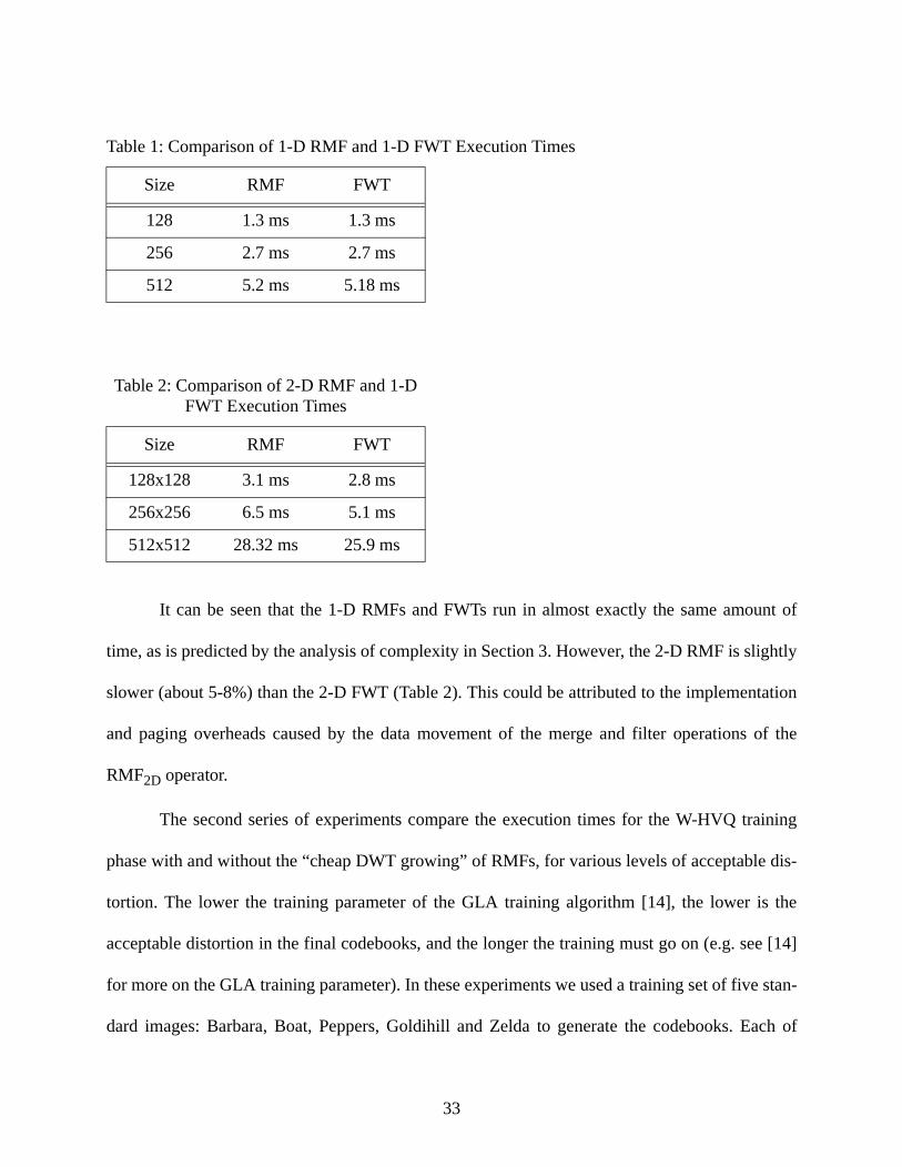
It can be seen that the 1-D RMFs and FWTs run in almost exactly the same amount of

time, as is predicted by the analysis of complexity in Section 3. However, the 2-D RMF is slightly

slower (about 5-8%) than the 2-D FWT (Table 2). This could be attributed to the implementation

and paging overheads caused by the data movement of the merge and filter operations of the

RMF2D operator.

The second series of experiments compare the execution times for the W-HVQ training

phase with and without the “cheap DWT growing” of RMFs, for various levels of acceptable dis-

tortion. The lower the training parameter of the GLA training algorithm [14], the lower is the

acceptable distortion in the final codebooks, and the longer the training must go on (e.g. see [14]

for more on the GLA training parameter). In these experiments we used a training set of five stan-

dard images: Barbara, Boat, Peppers, Goldihill and Zelda to generate the codebooks. Each of

Table 1: Comparison of 1-D RMF and 1-D FWT Execution Times

Size RMF FWT

128 1.3 ms 1.3 ms

256 2.7 ms 2.7 ms

512 5.2 ms 5.18 ms

Table 2: Comparison of 2-D RMF and 1-D FWT Execution Times

Size RMF FWT

128x128 3.1 ms 2.8 ms

256x256 6.5 ms 5.1 ms

512x512 28.32 ms 25.9 ms

33

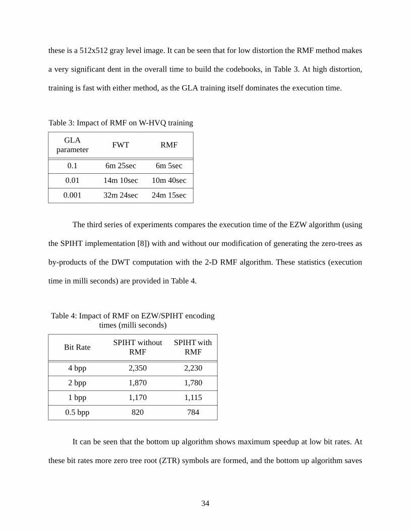
these is a 512x512 gray level image. It can be seen that for low distortion the RMF method makes

a very significant dent in the overall time to build the codebooks, in Table 3. At high distortion,

training is fast with either method, as the GLA training itself dominates the execution time.

The third series of experiments compares the execution time of the EZW algorithm (using

the SPIHT implementation [8]) with and without our modification of generating the zero-trees as

by-products of the DWT computation with the 2-D RMF algorithm. These statistics (execution

time in milli seconds) are provided in Table 4.

It can be seen that the bottom up algorithm shows maximum speedup at low bit rates. At

these bit rates more zero tree root (ZTR) symbols are formed, and the bottom up algorithm saves

Table 3: Impact of RMF on W-HVQ training

GLA parameter

FWT RMF

0.1 6m 25sec 6m 5sec

0.01 14m 10sec 10m 40sec

0.001 32m 24sec 24m 15sec

Table 4: Impact of RMF on EZW/SPIHT encoding times (milli seconds)

Bit RateSPIHT without

RMFSPIHT with

RMF

4 bpp 2,350 2,230

2 bpp 1,870 1,780

1 bpp 1,170 1,115

0.5 bpp 820 784

34

us the effort of searching the immediate children of these coefficients. At higher bit rates the zero

tree hypothesis is violated more often, which means that the immediate children of the high level

coefficients need to be examined and codes generated for them.

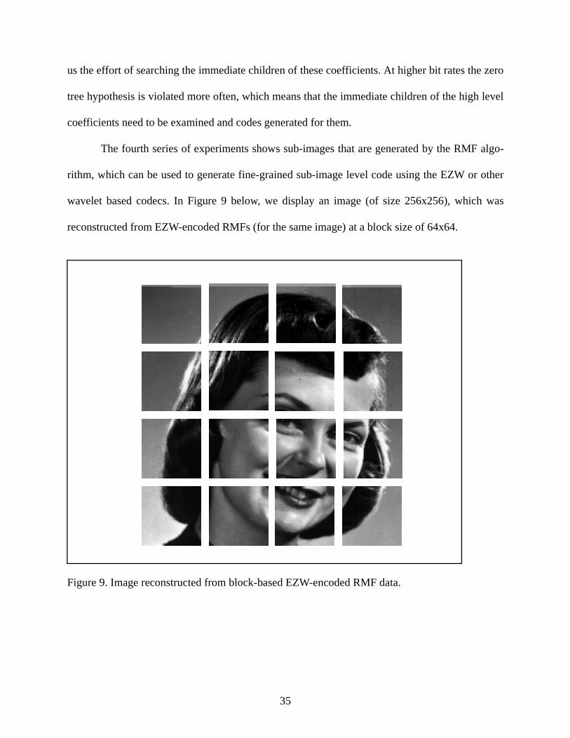
The fourth series of experiments shows sub-images that are generated by the RMF algo-

rithm, which can be used to generate fine-grained sub-image level code using the EZW or other

wavelet based codecs. In Figure 9 below, we display an image (of size 256x256), which was

reconstructed from EZW-encoded RMFs (for the same image) at a block size of 64x64.

Figure 9. Image reconstructed from block-based EZW-encoded RMF data.

35

6.0 Conclusions and Future Work

In this paper, we have proposed the Recursive Merge-Filter (RMF) algorithm for comput-

ing the Discrete Wavelet Transform, and shown that it has the nice properties of a data flow struc-

ture which is geometrically recursive, i.e. fractal in nature, and extends to higher dimensions.

Unlike the FWT, it has the nice property of maintaining spatial coherence with the input data, and

provides an extremely efficient way of building larger wavelet transforms from smaller ones,

without first inverting the smaller DWTs. We have demonstrated one application area (W-HVQ

training) where this “DWT growing” property can drastically reduce the computing time, and one

(EZW/SPIHT) in which the bottom-up tree growing nature of the RMF algorithm, combined with

the spatial coherence property of RMF can concurrently generate the zero tree significance map

as a by-product of the transform. We have also offered the new capability of fine-grained (or sub-

image level) wavelet coding, by using block-wise wavelet transforms (encoded with EZW) as an

alternative to the DCT in JPEG or MPEG codecs.

This work brings up several interesting possibilities for future research:

1) We propose to investigate extending the RMF algorithm to compute the inverse DWT. This

may be relevant for those kinds of DSP, where the preferred or “natural” domain is the transform

(e.g. frequency) domain, e.g. audio and control systems, and where one may be interested in the

intermediate results of taking the inverse transform. For orthogonal transforms, this extension of

the RMF is expected to be easy, as the computational structure is typically the same in both for-

ward and reverse directions for such transforms;

2) It would be interesting to characterize transforms that maintain spatial coherence, and the prop-

erties that they need to exhibit in order to use the RMF data flow, e.g. locality [7];

36

3) Look for ways of improving the performance of EZW, by utilizing the “smooth” coefficient

values at each step of the RMF transform algorithm in constructing the zero tree significance

maps. These values correspond to local spatial averages, which are not available in the final

DWT, at which point the EZW/SPIHT algorithms proposed in the literature start their encoding;

4) We propose to use the RMF algorithm instead of DCT, and the EZW encoding algorithm

instead of Huffman, thus giving new MPEG and JPEG codecs, which have the capability of gen-

erating fine grained (i.e sub-image level) codes, using wavelet transforms.

5) Our implementation of the 1-D and 2-D RMF operator is stateless. Thus, they are obliv-

ious to the type of overall computations for which they are being used, e.g. fine grained coding,

constructing larger DWTs by combining smaller ones, or in computing the end-to-end DWT of an

input array. This re-usable “black-box” design can be incorporated relatively easily into re-config-

urable hardware, parallel algorithms and large software systems in future research.

REFERENCES

[1]M. Vishwanath and P. Chou, “An Efficient Algorithm for Hierarchical Compression of Video”,

Proc. ICIP - 1994, Austin, Texas, vol. 111, pp. 275-279, November 1994.

[2]N.Chaddha, V.Mohan and P.Chou, “Hierarchical vector quantization of perceptually weighted

block transforms”, Proc. Data Compression Conference, IEEE, Piscataway, NJ, pp.3-12, 1995.

[3]J. Shapiro, “Embedded image coding using zero trees of wavelet coefficients”, IEEE Transac-

tions on Signal Processing, vol. 41, no. 12, pp. 3445-3462, December 1993

[4]W.H.Press, et.al., Numerical Recipes in C, 2nd edition, Cambridge University Press, 1992.

37

[5] S. G. Mallat, “A Theory for Multiresolution Signal Decomposition: The Wavelet Representa-

tion”, IEEE Transactions on Pattern Analysis and Machine Intelligence, vol.11, no.7, pp. 674-

693, July 1989.

[6] A. D. Poularikas, The Transforms and Applications Handbook, CRC Press Inc., 1996.

[7] M. Vetterli and J. Kovacevic, Wavelets and Subband Coding, Prentice Hall, 1995.

[8] A. Said and W. A. Pearlman, “A new fast and efficient image codec based on set partitioning

in hierarchical trees”, IEEE Transactions on Circuits and Systems for Video Technology, Vol. 6,

No. 6, pp. 243-250, June 1996.

[9] J. -R. Ohm, “Three-dimensional subband coding with motion compensation”, IEEE Transac-

tions on Image Processing, Vol. 3, No. 5, 1994.

[10] C. I. Podilchuk and R. J. Safranek, “Image and video compression: A review”, International

Journal of High Speed Electronics and Systems, Vol. 8, No.1, pp. 119-177, 1997.

[11]M. Vishwanath, “The Recursive Pyramid Algorithm for the Discrete Wavelet Transform”,

IEEE Transactions on Signal Processing, Vol. 42, No. 3, 1994.

[12]S.G. Mallat, A Wavelet Tour of Signal Processing, Academic Press, 1997.

[13]K.Mukherjee, “Image Compression and Transmission using Wavelets and Vector Quantiza-

tion”, Ph.D. thesis, University of Central Florida, 1999.

[14] A. Gersho, A. and R.M. Gray, Vector Quantization and Signal Compression, Kluwer Aca-

demic Publishers, 1992.

[15]R.M. Rao and A.S. Bopardikar, Wavelet Transforms: Introduction to Theory and Applica-

tions, Addison-Wesley Longman Inc., 1998.

38

[16]K. Sayood, Introduction to Data Compression, Morgan Kaufmann Publishers, Inc., 1996.

39