1

Recursive Decomposition

Richard PelikanOctober 10, 2005

Inference in Bayesian NetworksYou have a Bayesian network.

Let be a set of n discrete variablesWhat do you do with it?

QueriesAs we already know, the joint is modeled by

))(|(),...,,(1

21 ∏=

=n

iiin XparentsXPXXXP

},...,,{ 21 nXXXZ =

2

ConditioningWhen we want to explain a complex event in terms of simpler events, we “condition”.

Let , a set of instantiated variables. Let be the remaining variables in Z. Then,

Computing the probability of an event E

),()( EXPEPX∑=

))(|()(1∏∑=

=n

iii

XXparentsXPEP

ZE ⊆X

What is wrong?Solving the previous equation takes time which is exponential in X

We see this before we learn to “push in” summations.

Just to store a Bayesian network takes room, depending on the connectivity of the network

More parents means more table entries in the CPTs.

Bottom line: We have problems with time and space complexity.

3

ExampleYou have two emotional states (H). You have a pet rabbit (R).

Happy: your pet rabbit is alive.

Sad: your pet rabbit is dead.

R H

ExampleYour new neighbor is a crocodile farmer. If he farms (F), there is a risk of crocodile attack (C).

R HF C

4

ExampleYour new neighbor is a crocodile farmer. If he farms (F), there is a risk of crocodile attack (C).

The crocodile can eat your rabbit. You think you are scared of crocodile attacks.

R HF C

Example

More parents = more space.If we want to compute P(H), the computer does this:

0.90.1

0.20.8

R HF C

0.10.9

01

10

0.90.1

10

0.10.9

0.30.7FF

C

CC

F F C HHRR

C

CR

R

C

C

R

R

∑∑∑=F C R

CRHPCRPFCPFPHP ),|()|()|()()(

5

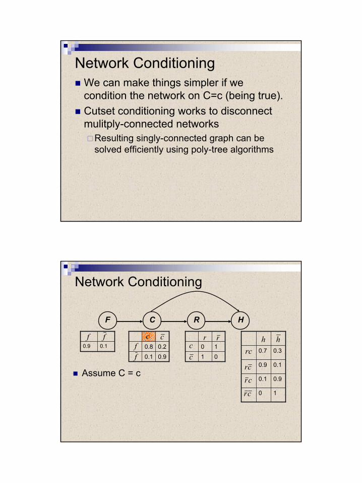
Network ConditioningWe can make things simpler if we condition the network on C=c (being true).Cutset conditioning works to disconnect mulitply-connected networks

Resulting singly-connected graph can be solved efficiently using poly-tree algorithms

Network Conditioning

Assume C = c

0.90.1

0.20.8

R HF C

0.10.9

01

10

0.90.1

10

0.10.9

0.30.7ff

c

cc

f f c hhrr

cr

rc

cr

cr

6

Network Conditioning

Assume C = cWe can save on space immediately –only half of the CPT for H is needed.

0.90.1

0.20.8

R HF C

0.10.9

01

10

0.20.8

10

0.90.1

0.30.7ff

c

cc

f f c hhrr

rc

cr

rc

rc

Network Conditioning

Assume C = cWe can save on space immediately–only half of the CPT for H is needed.The network is now singly connected. (Linear time and space complexity)

0.90.1

0.20.8

R HF C

0.10.9

01

10

0.90.1

0.30.7ff

c

cc

f f c hhrr

rc

cr

7

Network ConditioningWe can make things simpler if we condition the network on (being true).The result is a new, simpler network which allows any computation involving . Just as easily, another network can be created for and then we compute P(H) as the sum over conditions:

cC =cC =

cC =

∑ ∑∑

=

C F RRHPCRPFCPFPHP )|()|()|()()(

Network DecompositionInstead of worrying about single connectivity, it is easier to completely disconnect a graph into two subgraphs.Similar to tree-decomposition – which decomposition to pick?

We can use the BBN structure to decideAny decomposition works, but some are more efficient than others.

8

D-trees

D-Tree: full binary tree where leaves are network CPTsWe should decompose the original network by instantiating variables shared by left and right branches

0.90.1

0.20.8

R HF C

0.10.901

10

0.90.1

10

0.10.9

0.30.7

f

f c

c cf f chh

rr

cr

rc

cr

cr

C

F R

Decomposition

Smaller , less-connected networks are along the nodes of the d-tree

0.90.1

0.20.8

H

0.10.910

10

0.30.7

f

fc cf f c

hhrr

rc

cr

F C

RcC =F C

HR

9

Decomposition

∑ ∑∑

C F RRHPCRPFCPFP )|()|()|()(

∑F

FCPFP )|()(

H

F C

RF C

HR

The structure of the d-tree also shows how the computation can be factoredConditioning imposes independence between the variables in the factored portions of the graph

∑R

RHPRP )|()(

Factoring

All inference tasks are sums of products of conditional probabilities

F C HR

∑∏

∑∑∑

∈

=

=

FCR FCRiii

F C R

XparentsXP

CRHPCRPFCPFPHP

))(|(

),|()|()|()()(

10

Factoring

All inference tasks are sums of products of conditional probabilities

F C HR

∑ ∑∏

∑∏

∑∑∑

=

=

=

∈

∈

C FR FRiii

FCR FCRiii

F C R

XparentsXP

XparentsXP

CRHPCRPFCPFPHP

))(|(

))(|(

),|()|()|()()(

Factoring

At each step, you choose a new “cutset” and work with the subsequent networks

F C HR

∑ ∑∏∑∏

∑ ∑∏

∑∏

∑∑∑

=

=

=

=

∈∈

∈

∈

C R Riii

F Fiii

C FR FRiii

FCR FCRiii

F C R

XparentsXPXparentsXP

XparentsXP

XparentsXP

CRHPCRPFCPFPHP

))(|())(|(

))(|(

))(|(

),|()|()|()()(

11

Recursive Conditioning Algorithm

Cutsets

Conditioning on cutsets allow us to decompose the graph.

The union of all cutsets associated with T’s ancestor nodes

)()(var)(var)( TacutsetTsTsTcutset RL −= I

R HF C

C

F R

CRCF RHF

=)(Tacutset

12

23

12

45

34

67

56

1

78

32 4 5 86 71

1

2

3

4

5

6

7

Cutsets

23

12

45

34

67

56

1

78

32 4 5 86 71

1

2

3

4

5

6

7

Cutsets

23

12

45

34

67

56

1

78

1

12

123

1234

12345

123456

A-Cutsets

13

Some intuitionA cutset tells us what we are conditioning onAn A-cutset represents all of the variables being instantiated at that point on the d-tree.

We produce a solution for a subtree for every possible instantiation of the variables in the subtree’s A-cutset.There can be redundant computation

23

12

45

34

67

56

1

78

1

12

123

1234

12345

123456

A-Cutsets

ContextsSeveral variables in the acutset may never be used in the subtree.

14

23

12

45

34

67

56

1

78

1

12

123

1234

12345

123456

A-Cutsets

ContextsSeveral variables in the acutset may never be used in the subtree. We can instead remember the “context” under which any pair of computations yields the same result.

)()(vars)( TacutsetTTcontext I=

1

2

3

4

5

6

Contexts

Improved Recursive Conditioning Algorithm

15

Relation to Junction-Trees

Sepsets are equivalent to contexts Messages passed between links correspond to contextual information being passed upward in the d-treePassed messages sum out information about a residual (eliminated) set of variables – this is equivalent to the cutset.A d-tree can be built from a tree decomposition

SummaryRC operates in O(n exp(w)) time if you cache every context. This is better than being exponential in n. Caching can be selective, allowing the algorithm to run with limited memoryEliminates redundant computationIntuitively solves a complex event in terms of smaller events.