Recurring large deep earthquakes in Hindu Kushdriven by a sinking slabZhongwen Zhan1 and Hiroo Kanamori1

1Seismological Laboratory, Division of Geological and Planetary Sciences, California Institute of Technology, Pasadena,California, USA

Abstract Hindu Kush subduction zone produces large intermediate-depth earthquakes within a smallvolume every 10–15 years. Here we study the last three M ≥ 7 events within the cluster and find complexand diverse rupture processes. However, their main subevents appear to recur on the same fault patch,dipping 70° to the south. This recurrence requires an average of 9.6 cm/yr slip rate on the patch, much higherthan the ~1 cm/yr surface convergence rate measured geodetically. The high slip rate is likely caused bysignificant slab internal deformation, such as localized slab stretching/necking. We infer that the Hindu Kushsubducted slab below 210 km is sinking through the mantle at a vertical rate of 10 cm/yr.

1. Introduction

Hindu Kush is one of the most seismically active regions in the world, with frequent large (M≥ 7) earthquakesat about 200 km depth. The latest one was the 26 October 2015 Mw 7.5 earthquake, which caused >400casualties, only 13 years after the last Mw 7.3 earthquake in 2002 at almost the same location. The anoma-lously high seismic activity at depth has been noticed for a long time. For example, Gutenberg and Richter[1954] wrote in Seismicity of the Earth: “Among the Hindu Kush earthquakes at intermediate depth the largershocks are abnormally frequent, … Most of the epicenters are at nearly the same point near 36.5 N, 70.5 E(230 km).” The Global Centroid-Moment-Tensor (GCMT) catalog and the recently compiled ISC-GEM catalog[Storchak et al., 2013], in which large earthquakes’ locations and magnitudes are recalibrated with specialcare [Di Giacomo et al., 2015], show that M≥ 7 Hindu Kush deep earthquakes occurred semiregularly, onceevery 10–15 years (Figure 1). For 1900–1950, when the ISC-GEM catalog is not complete for M7s, theGutenberg-Richter catalog includes 10 more M7 events (gray dots in Figure 1b), suggesting that the activityprior to 1950 may have been even higher than recent years. However, the 10 events’magnitudes may not bewell calibrated.

TheHinduKush deep earthquakes are concentrated in a small volume (Figure 1a) andoften called “earthquakenest” [Pavlis and Hamburger, 1991; Pegler and Das, 1998; Pavlis and Das, 2000; Prieto et al., 2012]. In particular,Sippl et al. [2013] relocated small earthquakes in Hindu Kush from 2008 to 2010 using a local seismic networkand found that the deep events form a band only 15 km thick. For the M ≥ 7 events in the last century,epicenters and centroids from various catalogs are all located within 50 km from each other. A notable excep-tion is the 1983 Mw 7.4 GCMT centroid, which is offset to the north by >50 km, even though its epicenter inthe U.S. Geological Survey (USGS) Preliminary Determination of Epicenters (PDE) bulletin is still close to theother events (Figure 1a). In Figure 1c we compare the long-period (T> 20 s) waveforms between the 1983and the 2015 events at four stations, aligned on the direct Pwaves. We find that all the later phases includingsP, PP, S, SS, and surface waves are well aligned and have similar waveforms. If the 1983 centroid is actuallydisplaced from the other events as shown in Figure 1a, these later phases would have 5–10 s misalignments,easily visible in Figure 1c. Therefore, we conclude that the 1983 earthquake centroid location and depth arevery close to the other M> 7 events.

Why large deep earthquakes in Hindu Kush are so frequent and concentrated is unclear. The earthquakelocations and focal mechanisms suggest they are intraplate earthquakes within the subducted oceanic plate,loaded by slab pulling stress [Pegler and Das, 1998]. The plate convergence rate measured on the surface isvery low, only ~1 cm/yr, as part of the 3–5 cm/yr overall shortening distributed across a wide area [Ischuket al., 2013]. Therefore, significant slab internal deformation is required to cause the active seismicity. Listeret al. [2008] proposed that the Hindu Kush earthquake nest is a manifestation of active slab stretching(necking) due to the negative buoyancy of a hanging “slablet.” But the required slab-stretching rate is not

ZHAN AND KANAMORI RECURRING HINDU KUSH EARTHQUAKES 1

PUBLICATIONSGeophysical Research Letters

RESEARCH LETTER10.1002/2016GL069603

Key Points:• Large intermediate-depth earthquakesin Hindu Kush concentrate in a smallvolume

• The last three M ≥ 7 events showdiverse rupture processes, but theirmain subevents appear to recur onthe same fault patch

• The recurrence requires significantslab internal deformation such asnecking due to a fast sinking slab

Supporting Information:• Supporting Information S1

Correspondence to:Z. Zhan,zwzhan@gps.caltech.edu

Citation:Zhan, Z., and H. Kanamori (2016),Recurring large deep earthquakes inHindu Kush driven by a sinking slab,Geophys. Res. Lett., 43, doi:10.1002/2016GL069603.

Received 17 MAY 2016Accepted 29 JUN 2016Accepted article online 4 JUL 2016

©2016. American Geophysical Union.All Rights Reserved.

constrained, and whether the rate is physically plausible is unknown. To quantify the slab-stretching picture,in this paper we study the last threeM≥ 7 events with globally distributed digital seismic data in detail: the 9August 1993Mw 7.0 event, the 3 March 2002Mw 7.3 event, and the 26 October 2015Mw 7.5 event (Table S1 inthe supporting information). We aim to answer the following questions: Are the earthquakes recurring(at least partially) on the same fault plane?What is the average slip rate on the fault plane? Is the correspondingslab-stretching rate plausible for the slab negative buoyancy and mantle viscosity?

2. Depths and Focal Mechanisms

Earthquake depths are often difficult to constrain with only first-arrival data or long-period waveforms. TheGCMT solutions of the 1993, 2002, and 2015 events have similar horizontal locations (Figure 1a) but differentdepths: the difference in depth between the 2002 and 2015 events is more than 30 km (Figure 2a), too largefor the events to overlap significantly. To resolve whether the three events possibly ruptured the same faultplane, we first apply the cut-and-paste (CAP) method to determine their point source solutions [Zhu andHelmberger, 1996; Zhan et al., 2012]. We filter teleseismic P and SH waveforms with a pass band of 20–100 s,a period band long enough for the events to be approximated as point sources and short enough for the

Figure 1. Hindu Kush seismicity. (a) Earthquake locations in the Hindu Kush area. The small dots colored by depth are2008–2010 deep (>70 km) seismicity relocated by Sippl et al. [2013]. Five M> 7 earthquakes before 1983 in the ISC-GEMcatalog are displayed as gray squares, while the large gray square at (70.5°E, 36.5°N) contains 10 events located byGutenberg and Richter [1954]. The GCMT solutions and USGS PDE epicenters of the last four M> 7 events are shown aspurple dots and light blue stars, respectively. Because the 2002 and 2015M7 events are both registered as two earthquakes,there are two light blue stars for each event. The 1983 centroid is >50 km to the north of the other centroids, while itsepicenter does not have such an offset. The black star represents the 2009 reference event used in the directivity analysis.The gray rectangle marks the area plotted in Figure 4a. (b) Magnitude-time plot of M> 6.0 Hindu Kush deep earthquakes,based on the GCMT, ISC-GEM catalogs (red), and the Gutenberg-Richter catalog (gray). This study focuses on events withmagnitude around and above 7.0, which is marked by the gray dashed line. (c) Comparison of the long-period (T> 20 s)waveforms between the 1983M7.4 event and the 2015M7.5 event, at four stations. The waveforms are aligned on the Pwaves, and amplitudes are normalized. The perfect alignments in later phases suggest that the GCMT centroid location ofthe 1983 event in Figure 1a is mislocated.

Geophysical Research Letters 10.1002/2016GL069603

ZHAN AND KANAMORI RECURRING HINDU KUSH EARTHQUAKES 2

depth phases to be separate from the direct phases. Synthetic waveforms are computed using the PREMmodel. We then grid-search depths and focal mechanisms by best fitting the waveforms. Figure 2a showsthe misfit curves, and the optimal depths are 210 km for the 1993 and 2015 events, and 215 km for the2002 event, with a 5 km grid-search step size. The CAP-inverted focal mechanisms are similar to the GCMTmoment tensor solutions (Figure 2a inset), with one nodal plane dipping ~70° toward the south and anothernodal plane dipping ~20° toward the north. From this comparison we conclude that the three events havesimilar centroid locations, depths, and focal mechanisms.

However, the three events are not repeaters in the sense that their rupture patterns are identical. Figure 2bdisplays their broadband P displacement waveforms at the same station COLA. Besides the differences inearthquake moment, the three events do not have the same waveforms, suggesting that at least thekinematic rupture processes are different. Interestingly, the three events also all have weak but clear precur-sory arrivals (zoomed red traces in Figure 2b), while the 1983 event does not. Poli et al. [2016] report that theinitiation phase is inefficient in generating seismic waves. Rupture processes producing the weak precursorsare difficult to image, and the later main slip patches can potentially be far away from the earthquakehypocenters. We will need to derive subevent models to get a clearer image of their rupture processes. Wewill follow a two-step procedure: (1) display the dominant features in waveform data and determine thefirst-order rupture processes by directivity analysis and (2) use themodels produced in step 1 as initial modelsto conduct waveform inversions for subevent models.

3. Directivity Analysis

The directivity analysis performed in this study is similar to that described in Zhan et al. [2014]. As shown byFigure 3, we first arrange the teleseismic P waveforms by their horizontal directivity parameters defined by�cos(θ� θr)/cp, where θr is an assumed unilateral rupture direction from a reference point, θ and cp are

Figure 2. Point source solutions and broadband waveforms. (a) Cut-and-paste (CAP) inversion for the 1993, 2002, and 2015events and the 2009 reference event, using teleseismic P and SH waves. The dashed lines indicate the three large events’depths based on the GCMT catalog, different by more than 10 km between any pair. The dots connected by solid linesshow depthmisfit curves normalized by the optimal solutions, marked as larger dots. The optimal depths of the four eventsare within 5 km. The optimal focal mechanisms are shown in the inset, together with the GCMT moment tensors. (b)Broadband P displacement seismograms of the last four M ≥ 7 events recorded by station COLA, aligned by the onsets ofhigh-amplitude waves. The waveforms before the onsets are amplified by a factor of 10 to highlight the weak precursors.The numbers to the left of each trace are the amplification factors.

Geophysical Research Letters 10.1002/2016GL069603

ZHAN AND KANAMORI RECURRING HINDU KUSH EARTHQUAKES 3

station azimuth and P wave phase speed. Commonly, in directivity plots, the P waveforms are aligned at theonsets of P waves so that the epicenter is taken as the reference point. But if the P onsets are difficult to pickconsistently for all the stations due to noise or weak initiation phases, we may align the P waves by the the-oretical P arrival times corrected for the travel time anomaly along the path. Depending on how the traveltime predictions and path corrections are derived, the reference point in space maymove from the epicenter.If the assumed rupture direction, θr, is correct, subevents can be identified by straight lines with slopes givingthe distance of the subeventmeasured from the reference point in the azimuth of θr. For the three Hindu Kushevents, it is difficult to accurately pick the P onsets due to their weak initiation phases shown in Figure 2b.Furthermore, the relative locations of the USGS PDE epicenters may have large uncertainties, which makethe comparison among the three earthquakes ambiguous if we use the epicenter as the reference point.

We accordingly modify the directivity analysis using a nearby event as reference. As the reference event, weuse the 26 October 2009 Mw 6.2 earthquake (black star in Figure 1a) relocated by Sippl et al. [2013] using alocal seismic network. Our CAP inversion demonstrates that the 2009 event is similar to the three large eventsin depth and focal mechanism (Figure 2a) and serves as a good calibration event. To avoid involving rupturecomplexities within the 2009 event, we low-pass filter all the data at 3 s. Figure 3a shows the directivity plotfor the 2009 event, aligned at the largest phase by cross correlations. This plot is used to determine along-path travel time corrections. We then apply the travel time corrections to the directivity plots of the threelarge events. We align their P waveforms by the theoretical P travel times based on their own origin timesbut the 2009 event’s epicenter with the travel time corrections. Therefore, the reference points for all threelarge events are the same, at the 2009 epicenter. We grid-search rupture direction θr with a 2° interval andvisually inspect all the directivity plots for the θr range showing overall best linear alignments. The optimal

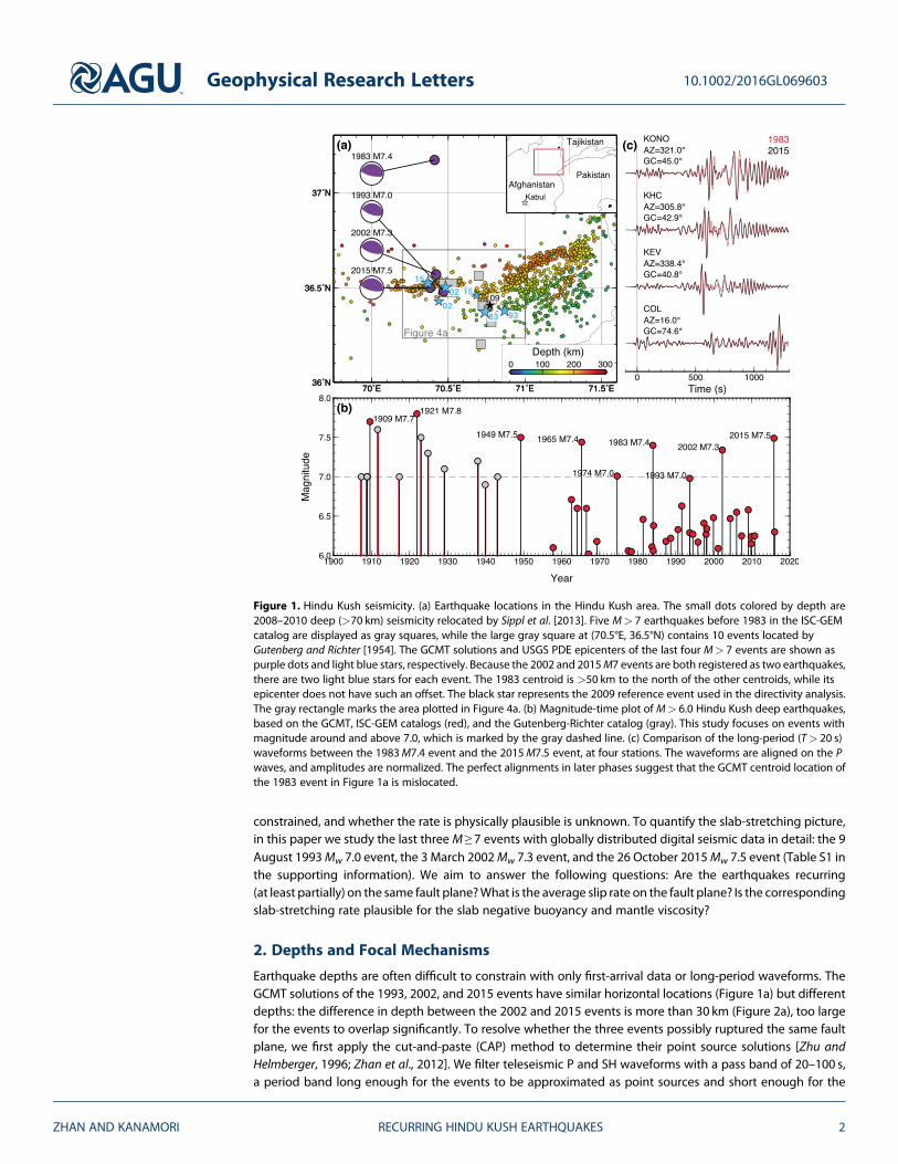
Figure 3. Directivity analysis. (a) Teleseismic P waveforms of the 2009 reference event, low-pass filtered at 3 s, and alignedby cross correlations. Station names and azimuths are shown to the left and right, respectively. (b–d) Directivity plots of the1993, 2002, and 2015 events, after applying the travel time corrections derived from the 2009 reference event in Figure 3a.The waveforms are arranged by their directivity parameters with the reference point at the relocated 2009 epicenter(instead of their own epicenters) and an assumed rupture azimuth of 120°. Seismograms are flipped to ensure consistentpolarities. The thick purple lines with “E” labels indicate arrivals of major subevents, and the black dashed lines with “P”labels are predicted arrivals of their USGS PDE solutions (two for the 2002 and 2015 events).

Geophysical Research Letters 10.1002/2016GL069603

ZHAN AND KANAMORI RECURRING HINDU KUSH EARTHQUAKES 4

θr is around 120°, roughly parallel to the fault strikes, and the directivity plots are displayed in Figures 3b–3d.For comparison, Figure S1 shows the directivity plots without travel time correction. The waveform align-ments shown in Figure 3 are much more coherent than the ones shown in Figure S1. Due to the change inthe reference points, the time axes in Figures 3 and S1 are somewhat arbitrary, but only the relative timingof subevents is important here.

The main P wave pulses of the 1993 Mw 7.0 earthquake are aligned vertically as subevent E1 (Figure 3b),which means that E1 is located close to the 2009 reference event. The predicted arrival times based on theUSGS PDE solution (light blue star in Figure 1a) are plotted as the black dashed line in Figure 3b, whichmatches the precursory arrivals well. About 5–10 s after E1, another (possibly two) group of coherent phasesarrive without aligning on straight lines, suggesting additional subevent(s) not located along the assumedrupture azimuth of 120°. Unfortunately, a major azimuthal gap makes it difficult to locate them accurately.

We identify three subevents for the2002Mw7.3 event (Figure3c). Subevent E1has anegative slope, suggestinga location about 30 km to the N60°W (opposite to the assumed θr) of the 2009 event. Later, large subevents E2and E3 both have nearly vertical alignments, hence are located near the 2009 event. Overall, the 2002 eventruptured unilaterally along the assumed θr, 120°. In the USGS PDE catalog, the 2002 event is registered as twoearthquakes (Figure 1a), whose predicted arrival times are plotted as the black dashed lines P1 and P2 inFigure 3c. While P1 is subparallel to E1, “mainshock” P2 is not parallel to E2 and E3 but has a negative slope.This appears to be a mislocation of the “mainshock” epicenter P2 caused by the difficulty in picking the“mainshock” onsets within the precursory arrivals from E1.

The 2015 Mw 7.5 event, with its 10 s long precursory arrivals, is also listed as two events, P1 and P2, in theUSGS PDE catalog (Figure 1a). Epicenter P1 is located close to the 2009 event, while epicenter P2 is ~30 kmtoward the west. This geometry is roughly consistent with subevents E1 and E2 (Figure 3d). A large subeventE3 occurred close to E2, but with a slightly steeper slope, implying a rupture backward to the east. Soon afterE3, subevent E4 ruptured back in the epicenter area close to the 2009 event, with a vertical moveout. Due tothe small temporal separation between E3 and E4, their waveformsmerge together at the stations toward theeast (bottom portion of Figure 3d).

In summary, the three events show diverse and complex rupture processes. The 1993 event had only weakdirectivity, the 2002 event ruptured mostly toward the east, and the 2015 event first ruptured toward thewest and then backward to the east. However, major arrivals in the directivity plots are aligned nearly verti-cally, suggesting major subevents of all three earthquakes locate close to the 2009 reference event, except2015.E3 to the west.

4. Subevent Models

While the directivity analysis reveals the essential features (e.g., main subevents, overall rupture directions) ofthe three events, quantitative details regarding the number of subevents, the precise locations, timings, andthe moments of the subevents must be derived from waveform inversion. Here we use a subevent algorithmsimilar to that in Zhan et al. [2014], to simultaneously invert the P waveforms shown in Figure 3 (after traveltime corrections) formultiple subevent centroid locations, centroid times, andmoments. For each set of sube-vent locations and times, we predict their arrival times at each station, and then assume Gaussian-shapedsource-time-functions (STFs) centered at the predicted times, and determine the best fitting durations andamplitudes. Subevent moment is calculated posteriorly as proportional to the area beneath its average STF.We refer the readers to Zhan et al. [2014] for more details on the method, and here we only note one changein this application. In Zhan et al. [2014], subevent durations and amplitudes are estimated independently foreach station to accommodate possible path and site effects. Because the velocity seismograms used hereare low-pass filtered at 3 s, the sharpness of pulses is largely smeared. Therefore, we simplify the method byassuming that observed subevent durations τij at the jth station from the ith subevent follow a cosine azimuthpattern τij= τi+Δτj cos(φj� φi), where τi is subevent duration, τj is station azimuth.We includeΔτj and φi as newvariables in the nonlinear inversion. This simplification improves the efficiency and robustness of inversions.

Figure 4a and Table S1 describe the subevent models. With three subevents for the 1993 and 2002 events,and four subevents for the 2015 event, we are able to fit the teleseismic P waveforms remarkably well (seeFigure 5). The 1993 event ruptured its largest M6.8 subevent E1 slightly south of the 2009 event, and then

Geophysical Research Letters 10.1002/2016GL069603

ZHAN AND KANAMORI RECURRING HINDU KUSH EARTHQUAKES 5

Figure 4. Subevent models and fault plane. (a) Subevents of the 1993, 2002, and 2015 earthquakes are shown as circlesnumbered sequentially, with sizes proportional to the subevent moments. Moment rate functions are displayed in thetop left in the same colors. Gray dots/squares (west/east of 70.85°E, respectively) and pink dots are the 2008–2010 relocatedseismicity and 2015 aftershocks, respectively, which are projected to profile AA′ in Figure 4b. The 2009 event on the profileAA′ (black star) serves as the origin point in Figure 4b. The projected events form two distinct structures dipping towardopposite directions: ~75° to the south for events west of 70.85°E (gray dots and the red dashed line), ~75° to the northfor events east of 70.85°E (gray squares). The south dipping plane is subparallel to the steeper nodal plane in the focalmechanism solutions (red line in the inset).

Figure 5. Waveform fits of subevent models for the (a) 1993Mw 7.0, (b) 2002Mw 7.3, and (c) 2015Mw 7.5 events. The direc-tivity parameters and alignments are the same as in Figure 3. Data and synthetics are plotted in black and red, respectively.

Geophysical Research Letters 10.1002/2016GL069603

ZHAN AND KANAMORI RECURRING HINDU KUSH EARTHQUAKES 6

two smaller subevents E2 and E3 to the north. The 2002 event initiated with an M6.6 subevent E1, and thenruptured to the east with a bigger subevent E2, and the biggest subevent E3 (M7.2) near the 2009 event. E3contributes most of the moment of the 2002 event. The 2015 event started with aM6.4 subevent E1 near the2009 event, and ruptured toward N60°W to E2, about 30 km away. Then the rupture reversed direction andproduced a M7.3 subevent E3. Two seconds after E3, another M7.2 subevent E4 occurred back near the2009 event. A continuous rupture from E2/E3 to E4 may be unlikely considering the short time delay, sowe consider E4 as a late development after E1, possibly with dynamic triggering from E2 or E3.

5. Fault Plane and Slip Rate

Despite the diverse rupture processes, the major subevent of each earthquake, 1993.E1, 2002.E3, and 2015.E4are all located within 5 km of the 2009 event, the spatial resolution of subevent modeling. With subeventstreated as point sources in our method, we cannot constrain their spatial dimensions. Therefore, to assesswhether the three subevents overlap significantly, we assume a circular crack and a constant strain drop of10�4, the average value commonly suggested for earthquakes at all depths [Vallée, 2013]. We then convertthe strain drop to stress drop using the shear modulus at 210 km depth in the PREM model, and estimatethe rupture dimensions and average slips from the subevent moments. For the M7.2 subevents 2002.E3and 2015.E4, the diameter of the fault is about 32 km and average slip is ~1.2m, while for the M6.8 1993.E1 the diameter is about 20 km, and average slip is ~0.7m. These diameters are much larger than the offsetsbetween the subevents. Together with the similar centroid depths and focal mechanisms estimated insection 2, we suggest that the three large subevents ruptured on the same (or closely spaced subparallel)fault patch, instead of side-by-side laterally.

The focal mechanisms estimated in section 2 suggest two possible fault planes, one dipping to the south at70°, the other to the north at 20°. The subevent models do not provide any additional constraints on whichfault plane the three large subevents recurred. In this case, we may use background seismicity and after-shocks to identify the fault plane. In Figure 4b, we project the relocated background seismicity and after-shocks of the 2015 event onto profile AA′, roughly perpendicular to the fault strikes. The projectedseismicity shows two clearly separated dipping structures toward the south and north, respectively, bothat ~75° (Figure 4b). Note that the events east of 70.85°E (gray squares) form the north dipping structure, whilethe events west of 70.85°E (gray dots), including the 2015 aftershocks (pink dots), form the south dippingstructure. Thus, we suggest that the south dipping nodal plan is the fault plane of the three large subevents.

Lister et al. [2008] show that deep earthquake locations and focal mechanisms in Hindu Kush support theslab-stretching model, in which earthquakes concentrate in the necking zone due to the ongoing break-off of the subducted oceanic slab. Given our new observation that M~ 7 subevents may recur on the samefault plane, what would be the required slab-stretching rate? To answer this question, we calculate the cumu-lative slip on the fault as a function of time (Figure 6a). As discussed above, the last threeM ≥ 7.0 events likelyproduced average slips of 0.7m (1993.E1) and 1.2m (2002.E3 and 2015.E4), respectively. We further assumethat the three earlier events, 1949M7.5, 1965M7.4, and 1983M7.4, are similar to the 2002M7.3 and 2015M7.5events, each contributing 1.2m of slip on the same fault patch, and the 1974M7.0 event is similar to the1993M7.0 event, contributing 0.7m slip. Combining all these events together, we have 6.2m cumulative slipin 66 years since the 1949 event. The best fitting average slip rate is about 9.6 cm/yr, as shown by the red linein Figure 6a. This slip rate on a 70° dipping fault translates to a vertical slab-stretching rate of 9 cm/yr, muchhigher than the convergence rate measured geodetically on the surface, at about 1 cm/yr [Ischuk et al., 2013].Therefore, the slab below the earthquake depth of 210 km needs to sink at 10 cm/yr to fuel the frequentlyrecurring M ≥ 7.0 deep earthquakes (sketched in Figure 6b). If additional aseismic deformation is involved,then the slab-sinking speed will be higher.

Slab negative buoyancy and mantle viscosity control slab-sinking speed. Seismic tomographic models showthat the Hindu Kush subducted slab has not reached the high-viscosity lower mantle yet, as sketched inFigure 6b based on Figure 2 of Negredo et al. [2007]. If we assume that the slab necking zone is not providingsignificant resistance, then we can do back-of-envelope calculations about the required mantle viscosity forthe slab to be sinking at 10 cm/yr. We assume the process is close to a Stokes flow, with a higher density sphere

dropping through viscous fluid [Morgan, 1965]. The terminal sinking speed is given by v ¼ 2Δρ9μ gR2, in which

Δρ is density contrast, μ is viscosity, g is the gravitational acceleration, and R is radius of sphere. If we take the

Geophysical Research Letters 10.1002/2016GL069603

ZHAN AND KANAMORI RECURRING HINDU KUSH EARTHQUAKES 7

average slab density anomaly to be 0.5–1%, and sphere radius to be 100 km based on tomography [Negredoet al., 2007], the 10 cm/yr sinking speed requires a mantle viscosity of about 2 × 1020 Pa s. This value has theright order of magnitude for the upper mantle, especially for an active subduction zone [Alisic et al., 2012], butis a few times lower than those measured from postglacial rebound in cratonic regions [Turcotte and Schubert,2014]. Thus, the 10 cm/yr slab-stretching rate is physically plausible.

6. Conclusions

Out of the concentrated and anomalously frequent large deep earthquakes in Hindu Kush, we have studiedthe latest three M ≥ 7.0 events in 1993, 2002, and 2015 in detail. The three events show complex and diverserupture processes, but the main subevents/slips seem to always recur on the same fault patch, dipping 70° tothe south. To explain the 10–15 year intervals between theM~7 subevents, the average slip rate on the faultpatch needs to be ~9.6 cm/yr, much higher than the ~1 cm/yr convergence rate measured on the surface.The high slip rate is likely fueled by localized slab stretching/necking [Lister et al., 2008]. This requires the sub-ducted slab below 210 km to sink at a vertical rate of 10 cm/yr, which appears to be geodynamically plausible.The inferred slab stretching may be a transient process; as the slab eventually breaks off, the seismic activitywill cease and the surface will rebound [Richards and Hager, 1984; Duretz et al., 2011].

ReferencesAlisic, L., M. Gurnis, G. Stadler, C. Burstedde, and O. Ghattas (2012), Multi-scale dynamics and rheology ofmantle flowwith plates, J. Geophys. Res.,

117, B10402, doi:10.1029/2012JB009234.Di Giacomo, D., I. Bondár, D. A. Storchak, E. R. Engdahl, P. Bormann, and J. Harris (2015), ISC-GEM: Global instrumental earthquake catalogue

(1900–2009): III. Re-computed MS and mb, proxy MW, final magnitude composition and completeness assessment, Phys. Earth Planet. Inter.,239, 33–47.

Duretz, T., T. V. Gerya, and D. A. May (2011), Numerical modelling of spontaneous slab breakoff and subsequent topographic response,Tectonophysics, 502(1), 244–256.

Gutenberg, B., and C. F. Richter (1954), Seismicity of the Earth and Associated Phenomena, 2nd ed., Princeton Univ. Press, N. J.Ischuk, A., R. Bendick, A. Rybin, P. Molnar, S. F. Khan, S. Kuzikov, S. Mohadjer, U. Saydullaev, Z. Ilyasova, and G. Schelochkov (2013), Kinematics

of the Pamir and Hindu Kush regions from GPS geodesy, J. Geophys. Res. Solid Earth, 118, 2408–2416, doi:10.1002/jgrb.50185.Lister, G., B. Kennett, S. Richards, and M. Forster (2008), Boudinage of a stretching slablet implicated in earthquakes beneath the Hindu Kush,

Nat. Geosci., 1(3), 196–201.Morgan, W. J. (1965), Gravity anomalies and convection currents: 1. A sphere and cylinder sinking beneath the surface of a viscous fluid,

J. Geophys. Res., 70(24), 6175–6187, doi:10.1029/JZ070i024p06175.Negredo, A. M., A. Replumaz, A. Villaseñor, and S. Guillot (2007), Modeling the evolution of continental subduction processes in the Pamir–Hindu

Kush region, Earth Planet. Sci. Lett., 259(1), 212–225.

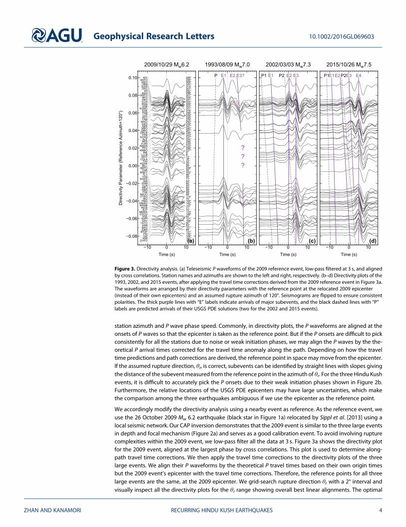
Figure 6. Slip rate and conceptual model. (a) Cumulative slip on the south dipping fault patch responsible for the mainsubevents of the 1993, 2002, and 2015 earthquakes. The step sizes for the three events are estimated based on subeventmoments and a constant strain drop of 10�4. If we assume that the earlier M ≥ 7 events since 1949 produced similarsubevents on the same fault patch, then we can extend to dashed lines. The red line shows the average slip rate of9.6 cm/yr, much faster than the ~1 cm/yr convergence rate measured on the surface. (b) Conceptual model to explain thehigh slip rate as slab-stretching/necking effect under its negative buoyancy. The geometry of the sinking slab below thenecking depth is based on the tomographic image in Negredo et al. [2007]. The green zone is sketched to illustrate slabgeometry with no stretching, as a comparison. The slab-sinking rate needs to be 10 cm/yr to explain the average slip rate onthe fault and the frequent large deep earthquakes.

Geophysical Research Letters 10.1002/2016GL069603

ZHAN AND KANAMORI RECURRING HINDU KUSH EARTHQUAKES 8

AcknowledgmentsIncorporated Research Institutions forSeismology (IRIS) provided the seismicdata used in this study. We thankThorne Lay and Lingling Ye forconstructive discussions, and twoanonymous reviewers for comments.

Pavlis, G. L., and M. W. Hamburger (1991), Aftershock sequences of intermediate-depth earthquakes in the Pamir-Hindu Kush seismic zone,J. Geophys. Res., 96(B11), 18,107–18,117, doi:10.1029/91JB01510.

Pavlis, G. L., and S. Das (2000), The Pamir-Hindu Kush seismic zone as a strain marker for flow in the upper mantle, Tectonics, 19(1), 103–115,doi:10.1029/1999TC900062.

Pegler, G., and S. Das (1998), An enhanced image of the Pamir–Hindu Kush seismic zone from relocated earthquake hypocentres, Geophys. J. Int.,134(2), 573–595.

Poli, P., G. Prieto, E. Rivera, and S. Ruiz (2016), Earthquakes initiation and thermal shear instability in the Hindu-Kush intermediate-depth nest,Geophys. Res. Lett., 43, 1537–1542, doi:10.1002/2015GL067529.

Prieto, G. A., G. C. Beroza, S. A. Barrett, G. A. López, and M. Florez (2012), Earthquake nests as natural laboratories for the study ofintermediate-depth earthquake mechanics, Tectonophysics, 570, 42–56.

Richards, M. A., and B. H. Hager (1984), Geoid anomalies in a dynamic Earth, J. Geophys. Res., 89(B7), 5987–6002, doi:10.1029/JB089iB07p05987.Sippl, C., B. Schurr, X. Yuan, J. Mechie, F. Schneider, M. Gadoev, S. Orunbaev, I. Oimahmadov, C. Haberland, andU. Abdybachaev (2013), Geometry

of the Pamir-Hindu Kush intermediate-depth earthquake zone from local seismic data, J. Geophys. Res. Solid Earth, 118, 1438–1457,doi:10.1002/jgrb.50128.

Storchak, D. A., D. Di Giacomo, I. Bondar, E. R. Engdahl, J. Harris, W. H. K. Lee, A. Villasenor, and P. Bormann (2013), Public release of the ISC-GEMglobal instrumental earthquake catalogue (1900–2009), Seismol. Res. Lett., 84(5), 810–815.

Turcotte, D. L., and G. Schubert (2014), Geodynamics, Cambridge Univ. Press, Cambridge, U. K.Vallée, M. (2013), Source time function properties indicate a strain drop independent of earthquake depth and magnitude, Nat. Commun., 4.Zhan, Z., D. Helmberger, M. Simons, H. Kanamori, W. Wu, N. Cubas, Z. Duputel, R. Chu, V. C. Tsai, and J.-P. Avouac (2012), Anomalously steep

dips of earthquakes in the 2011 Tohoku-Oki source region and possible explanations, Earth Planet. Sci. Lett., 353, 121–133.Zhan, Z., H. Kanamori, V. C. Tsai, D. V. Helmberger, and S. Wei (2014), Rupture complexity of the 1994 Bolivia and 2013 Sea of Okhotsk deep

earthquakes, Earth Planet. Sci. Lett., 385, 89–96.Zhu, L., and D. V. Helmberger (1996), Advancement in source estimation techniques using broadband regional seismograms, Bull. Seismol.

Soc. Am., 86(5), 1634–1641.

Geophysical Research Letters 10.1002/2016GL069603

ZHAN AND KANAMORI RECURRING HINDU KUSH EARTHQUAKES 9