Embed Size (px)
Citation preview

Recommender Systems
Jee-Hyong Lee
Department of Computer Science & Engineering
Sungkyunkwan University

Outline
1. Introduction
2. Collaborative Filtering Overview
3. Memory based Collaborative Filtering
4. Model based Collaborative Filtering
5. Content based Recommender System
6. Summary
2
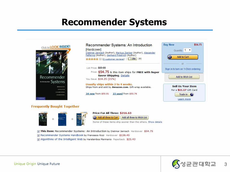
Recommender Systems
3

Recommender Systems
Netflix:
– 2/3 of the movies watched are recommended
Google News:
– Recommendations generate 38% more clickthrough
Amazon:
– 35% sales from recommendations
Choicestream:
– 28% of the people would buy more music if they found what they liked
4

Definition of Recommender Systems
Given
– User profile (usage history, demographics, …)
– Items (with or without additional information)
Goal
– Relevance scores of unseen items
– List of unseen items
By using a number of technologies
– Information Retrieval: document models, similarity, ranking
– Machine Learning & Data Mining: classification, clustering, regression, probability, association
– Others: user modeling, HCI
5
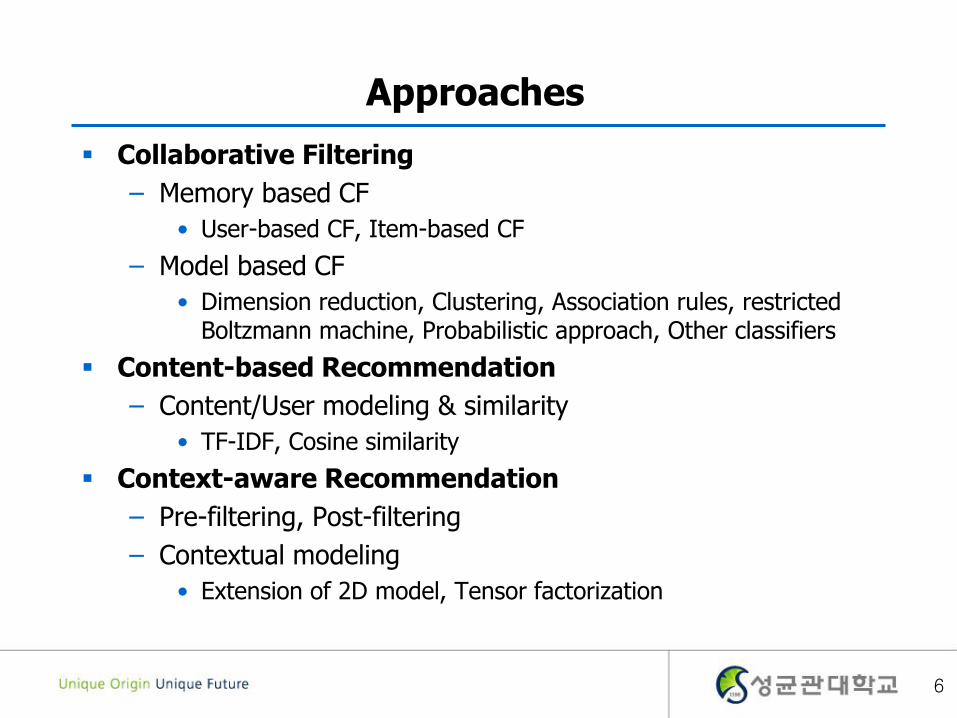
Approaches
Collaborative Filtering
– Memory based CF
• User-based CF, Item-based CF
– Model based CF
• Dimension reduction, Clustering, Association rules, restricted Boltzmann machine, Probabilistic approach, Other classifiers
Content-based Recommendation
– Content/User modeling & similarity
• TF-IDF, Cosine similarity
Context-aware Recommendation
– Pre-filtering, Post-filtering
– Contextual modeling
• Extension of 2D model, Tensor factorization
6

Approaches
Other Approaches
– Combining Multiple Recommendation Approach
– Combining Multiple Information
• Hybrid Information Network based CF
• Collective matrix factorization
– Diversity in Recommendation
– Division of Profiles into Sub-Profiles
– Recommendation for group users
7

Outline
1. Introduction
2. Collaborative Filtering Overview
3. Memory based Collaborative Filtering
4. Model based Collaborative Filtering
5. Content based Recommender System
6. Summary
8

Overview
Basic assumption and idea
– Implicit or explicit user ratings to items are available
– Customers who had similar tastes in the past, will have similar tastes in the future
I1 I2 I3 I4 I5
Active 5 3 ? 4
U1 2 2 3 3
U2 3 2 5 4
U3 4 3 2
U4 1 4
9

Overview
Easy to apply any domain
– Based on big data: commercial e‐commerce sites
– Easy to explain: wisdom of the crowd
– Flexible: various algorithms exist
– Example: book, movies, DVDs, ..
10
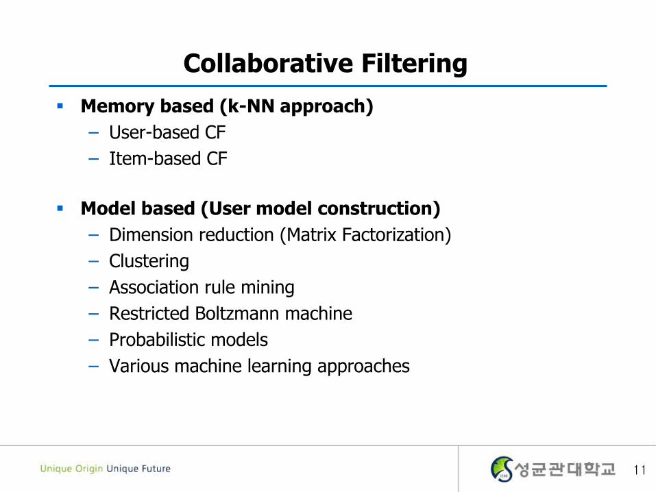
Collaborative Filtering
Memory based (k-NN approach)
– User-based CF
– Item-based CF
Model based (User model construction)
– Dimension reduction (Matrix Factorization)
– Clustering
– Association rule mining
– Restricted Boltzmann machine
– Probabilistic models
– Various machine learning approaches
11
Outline
1. Introduction
2. Collaborative Filtering Overview
3. Memory based Collaborative Filtering
3-1. User-based CF
3-2. Item-based CF
4. Model based Collaborative Filtering
5. Content based Recommender System
6. Summary
12
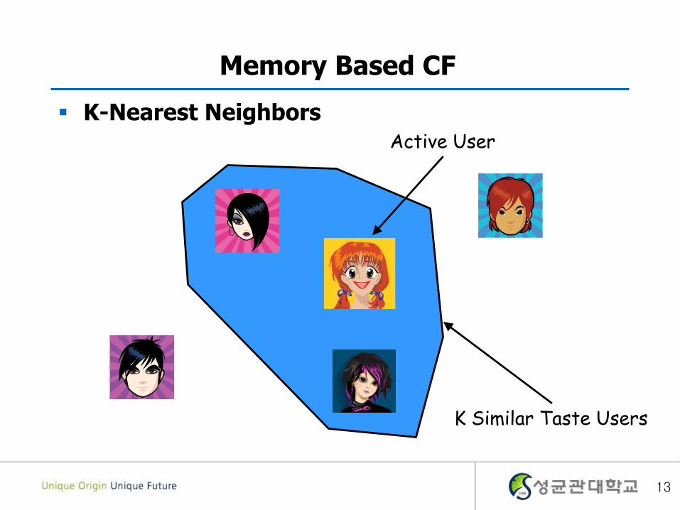
K-Nearest Neighbors
K Similar Taste Users
Memory Based CF
Active User
13

User-based Collaborative Filtering
Questions
– How to determine the similarity of two users?
– How to predict Active user’s rating using neighbors’ ratings?
I1 I2 I3 I4 I5
Active 5 3 ? 4
U1 2 2 3 3
U2 3 2 5 4
U3 4 3 2
U4 1 4
14

User-based Collaborative Filtering
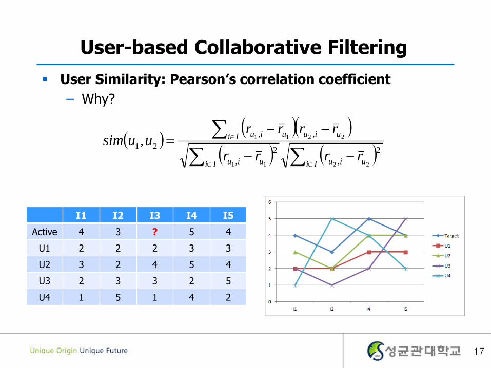
User Similarity: Pearson’s correlation coefficient
– : rating of user u for item i
– : user u’s average ratings
– I: items commonly consumed by u1 and u2
Ii uiuIi uiu
Ii uiuuiu
rrrr
rrrruusim
2
,
2
,
,,
21
2211
2211,
uriur ,
15
User-based Collaborative Filtering
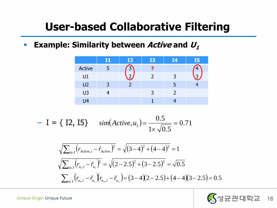
Example: Similarity between Active and U1
– I = { I2, I5} 71.05.01
5.0, 1
uActivesim
14443222
, Ii ActiveiActive rr
5.05.235.22222
, 11 Ii uiu rr
5.05.23445.22432211 ,, Ii uiuuiu rrrr
16
User-based Collaborative Filtering
User Similarity: Pearson’s correlation coefficient
– Why?
Ii uiuIi uiu
Ii uiuuiu
rrrr
rrrruusim
2
,
2
,
,,
21
2211
2211,
I1 I2 I3 I4 I5
Active 4 3 ? 5 4
U1 2 2 2 3 3
U2 3 2 4 5 4
U3 2 3 3 2 5
U4 1 5 1 4 2
17

User-based Collaborative Filtering
How much target user likes I3?
I1 I2 I3 I4 I5
Active 5 3 ? 4
U1 2 2 3 3
U2 3 2 5 4
U3 4 3 2
U4 1 4
itemscommon no available;Not ,
00.1,
not watch does available;Not ,
71.0,
3
3
322
1
uActivesim
uActivesim
IuuActivesim
uActivesim
18
User-based Collaborative Filtering
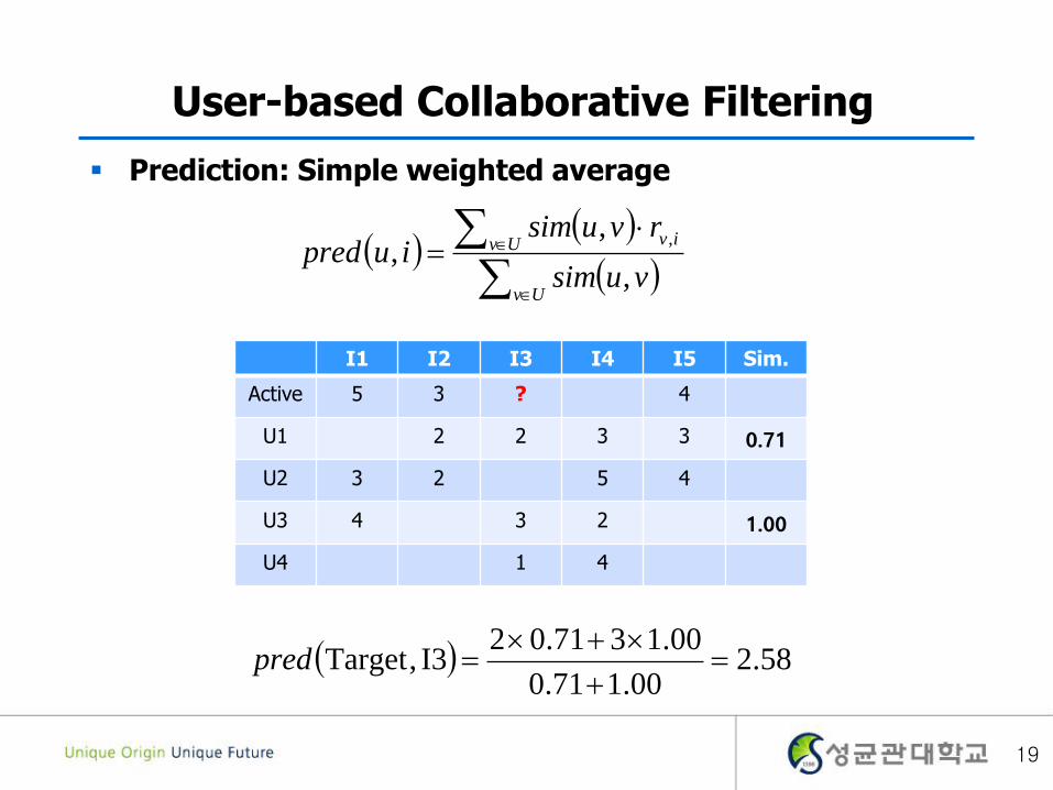
Prediction: Simple weighted average
Uv
Uv iv
vusim
rvusimiupred
,
,,
,
I1 I2 I3 I4 I5 Sim.
Active 5 3 ? 4
U1 2 2 3 3 0.71
U2 3 2 5 4
U3 4 3 2 1.00
U4 1 4
58.200.171.0
00.1371.02I3,Target
pred
19

User-based Collaborative Filtering
Prediction: Considering user bias
Uv
Uv viv
uvusim
rrvusimriupred
,
,,
,
I1 I2 I3 I4 I5 Sim.
Active 5 3 ? 4
U1 2 2 3 3 0.71
U2 3 2 5 4
U3 4 3 2 1.00
U4 1 4
79.300.171.0
00.13371.05.224I3,Target
pred
20

User-based Collaborative Filtering
How many neighbors?
– Only consider positively correlated neighbors (or higher threshold)
– Can be optimized based on data set
– Often, between 50 and 200
21

User-based Collaborative Filtering
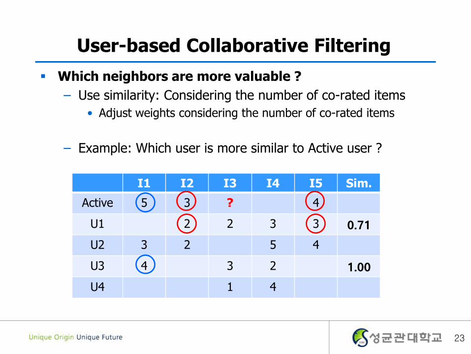
Which neighbors are more valuable ?
– User similarity: Different weights for items
• Give more weight to items with a higher variance
– Example: Which user is more similar to Active user ?
I1 I2 I3 I4 I5
Active 5 3 ? 4 5
U1 3 2 4
U2 5 4 5
U3 5 4 2 5
U4 5 1 5 5
22
User-based Collaborative Filtering
Which neighbors are more valuable ?
– Use similarity: Considering the number of co-rated items
• Adjust weights considering the number of co-rated items
– Example: Which user is more similar to Active user ?
I1 I2 I3 I4 I5 Sim.
Active 5 3 ? 4
U1 2 2 3 3 0.71
U2 3 2 5 4
U3 4 3 2 1.00
U4 1 4
23
User-based Collaborative Filtering
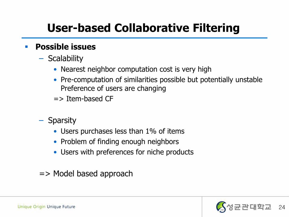
Possible issues
– Scalability
• Nearest neighbor computation cost is very high
• Pre-computation of similarities possible but potentially unstablePreference of users are changing
=> Item-based CF
– Sparsity
• Users purchases less than 1% of items
• Problem of finding enough neighbors
• Users with preferences for niche products
=> Model based approach
24

K items chosen bysimilar taste users
Item-based Collaborative Filtering
K Nearest Neighbors
Target Item
25

Item-based Collaborative Filtering
Questions
– How to determine the similarity of two items?
– How to predict Active user’s rating using neighbors’ ratings?
I1 I2 I3 I4 I5
Active 5 3 ? 4
U1 2 4 3
U2 2 2 5 3
U3 3 5 4
U4 1 3 2
26

Item-based Collaborative Filtering
Similarity between items: Pearson correlation
– : rating of user u for item i
– : item i’s average ratings
– U: users commonly consumed i1 and i2
Uu iiuUu iiu
Uu iiuiiu
rrrr
rrrriisim
2
,
2
,
,,
21
2211
2211,
iriur ,
27

Item-based Collaborative Filtering
Similarity between items
– Cosine similarity
– Adjusted cosine similarity
• Considering user bias
Uu iuUu iu
Uu iuiu
rr
rriisim
2
,
2
,
,,
21
21
21,
Uu uiuUu uiu
Uu uiuuiu
rrrr
rrrriisim
2
,
2
,
,,
21
21
21,
28
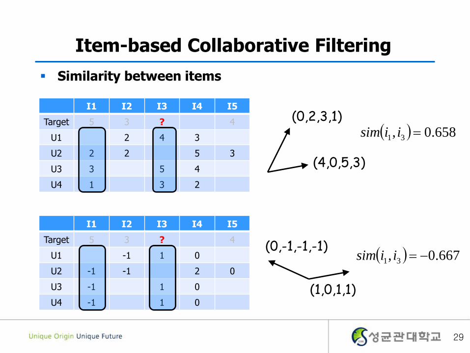
Item-based Collaborative Filtering
Similarity between items
I1 I2 I3 I4 I5
Target 5 3 ? 4
U1 2 4 3
U2 2 2 5 3
U3 3 5 4
U4 1 3 2
I1 I2 I3 I4 I5
Target 5 3 ? 4
U1 -1 1 0
U2 -1 -1 2 0
U3 -1 1 0
U4 -1 1 0
(0,2,3,1)
(4,0,5,3)
(0,-1,-1,-1)
(1,0,1,1)
658.0, 31 iisim
667.0, 31 iisim
29
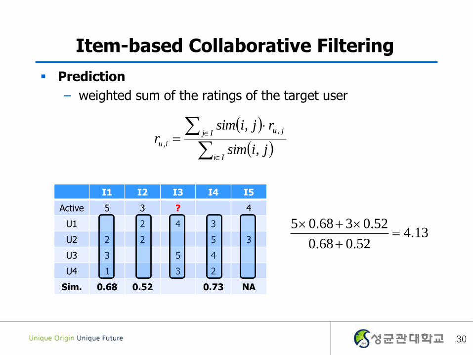
Item-based Collaborative Filtering
Prediction
– weighted sum of the ratings of the target user
Ii
Ij ju
iujisim
rjisimr
,
, ,
,
I1 I2 I3 I4 I5
Active 5 3 ? 4
U1 2 4 3
U2 2 2 5 3
U3 3 5 4
U4 1 3 2
Sim. 0.68 0.52 0.73 NA
13.452.068.0
52.0368.05
30
Item-based Collaborative Filtering
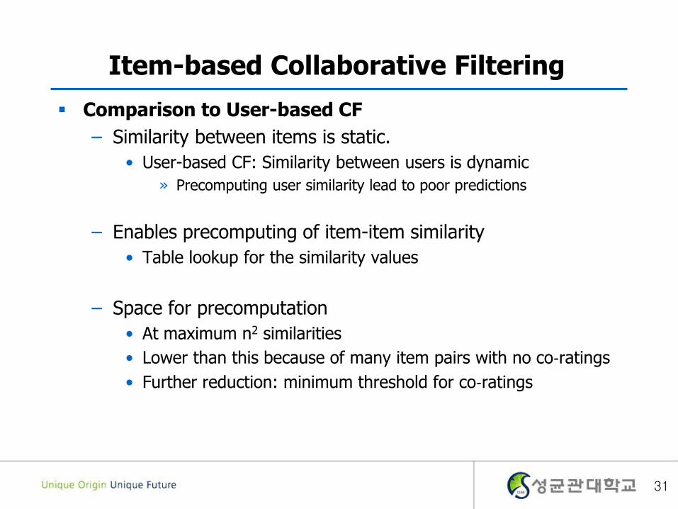
Comparison to User-based CF
– Similarity between items is static.
• User-based CF: Similarity between users is dynamic
» Precomputing user similarity lead to poor predictions
– Enables precomputing of item-item similarity
• Table lookup for the similarity values
– Space for precomputation
• At maximum n2 similarities
• Lower than this because of many item pairs with no co‐ratings
• Further reduction: minimum threshold for co‐ratings
31

Outline
1. Introduction
2. Collaborative Filtering Overview
3. Memory based Collaborative Filtering
4. Model based Collaborative Filtering4-1. Overview
4-2. Matrix Factorization
4-3. Singular Value Decomposition (SVD)
4-4. Prediction with SVD
4-5. Matrix Factorization through Optimization
5. Content based Recommender System
6. Summary
32
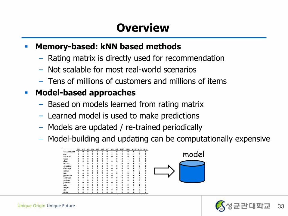
Overview
Memory-based: kNN based methods
– Rating matrix is directly used for recommendation
– Not scalable for most real-world scenarios
– Tens of millions of customers and millions of items
Model-based approaches
– Based on models learned from rating matrix
– Learned model is used to make predictions
– Models are updated / re-trained periodically
– Model-building and updating can be computationally expensive
33
model
Overview
Basic Techniques
– Dimension reduction (Matrix Factorization)
– Clustering
– Association rule mining
– Restricted Boltzmann machine
– Probabilistic models
– Various machine learning approaches
34

Matrix Factorization
Netflix 100M data
– Possibly 8,500M ratings (500,000 x 17,000)
– But, there are only 100 M non-zero ratings
Methods of dimensionality reduction
– Matrix Factorization
– Clustering
– Projection (PCA…)
Space complexity
– Worst case: O(mn)
– In practice: O(m + n)
35

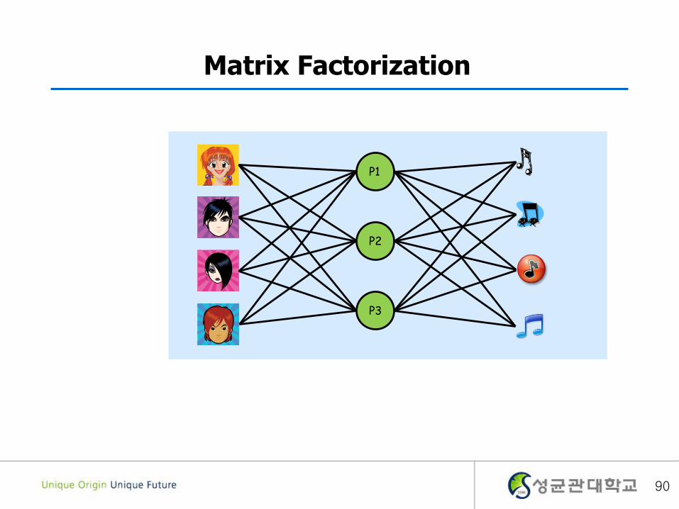
Matrix Factorization
Assume some latent factors in user preference
User 1 watched Item 1 User 1 likes RomanceItem 1 is RomanceSo, User 1 watched Item1
Unfortunately, we do not know about such latent factors !!
36
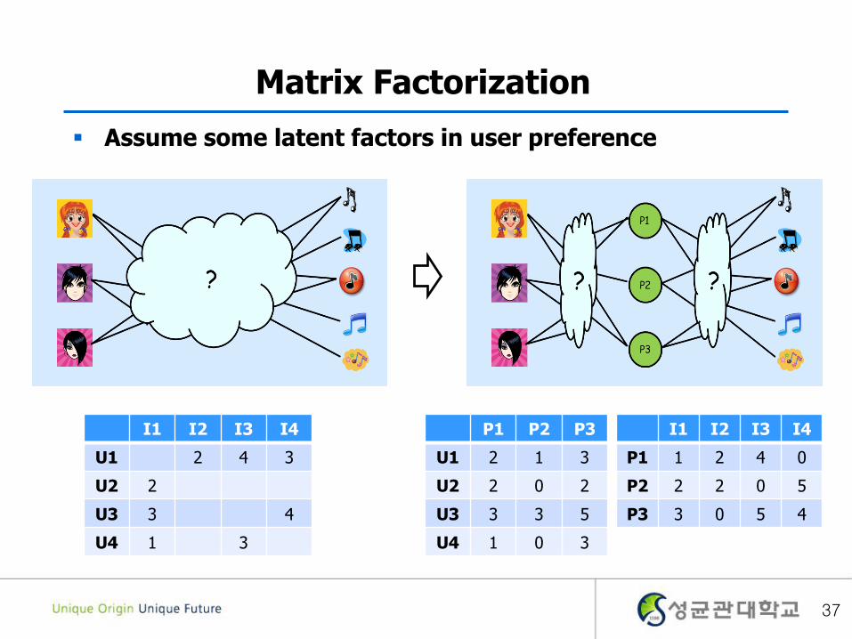
Matrix Factorization
Assume some latent factors in user preference
I1 I2 I3 I4
U1 2 4 3
U2 2
U3 3 4
U4 1 3
P1 P2 P3
U1 2 1 3
U2 2 0 2
U3 3 3 5
U4 1 0 3
I1 I2 I3 I4
P1 1 2 4 0
P2 2 2 0 5
P3 3 0 5 4
37

Matrix Factorization
Assume some latent factors in user preference
P1
P2
P3
1
2
3
2
3
1
1*2 + 2*3 + 3*1 = 11
11
P1 P2 P3
U1 1 2 3
U2
U3
U4
I1 I2 I3 I4
P1 2
P2 3
P3 1
38

Matrix Factorization
Assume some latent factors in user preference
I1 I2 I3 I4
U1 -0.061 1.791 4.048 3.062
U2 1.853 -0.493 0.113 0.141
U3 3.052 0.182 -0.041 3.947
U4 1.091 0.307 2.932 -0.088
P1 P2 P3
U1 -1.915 0.981 -0.524
U2 -0.267 -0.563 0.887
U3 -1.468 -1.581 -0.128
U4 -0.834 0.71 1.146
I1 I2 I3 I4
P1 -0.875 -0.58 -1.543 -1.764
P2 -1.204 0.459 1.413 -0.788
P3 1.061 -0.439 0.56 -0.872
I1 I2 I3 I4
U1 2 4 3
U2 2
U3 3 4
U4 1 3
39

Matrix Factorization
However, we do not know about latent factors
– We just blindly decompose the matrix
– Try to find and so that
I1 I2 I3 I4
U1 2 4 3
U2 2
U3 3 4
U4 1 3
P1 P2 P3
U1 2 1 3
U2 2 0 2
U3 3 3 5
U4 1 0 3
I1 I2 I3 I4
P1 1 2 4 0
P2 2 2 0 5
P3 3 0 5 4
NPPMNM IUR
NPI PMU NPPMNM IUR
= X? ?M
N N
M
P
P
40

Singular Value Decomposition
Any matrix can be decomposed into
U S V
41
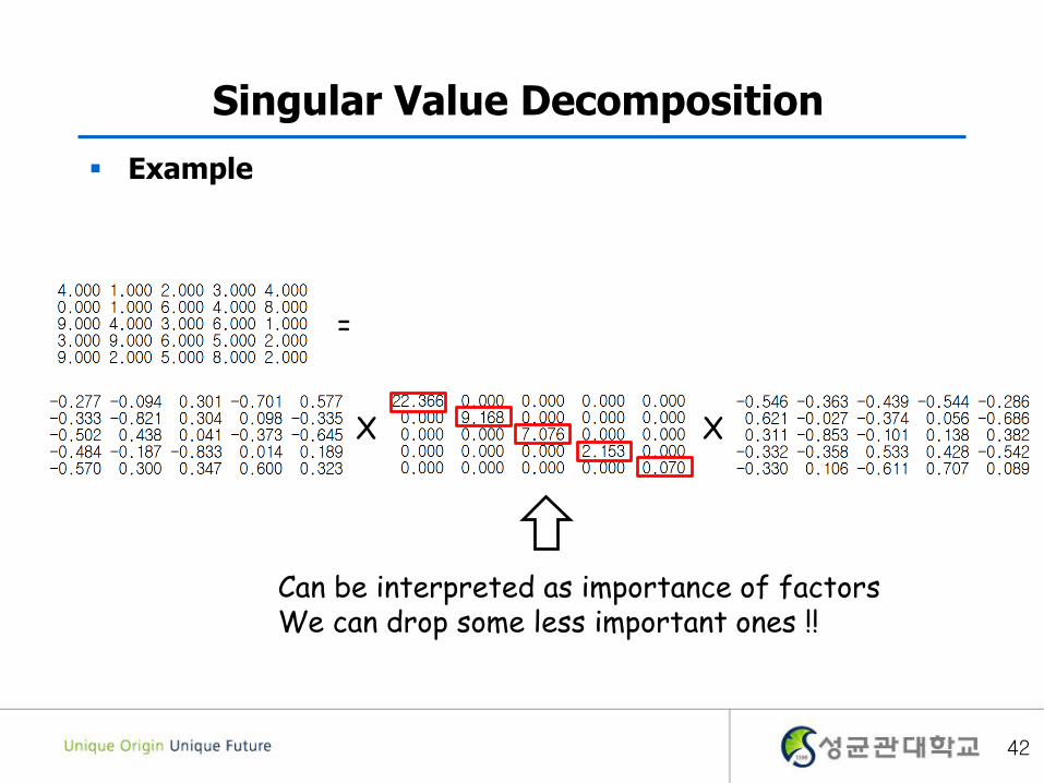
Singular Value Decomposition
Example
=
X X
Can be interpreted as importance of factorsWe can drop some less important ones !!
42

Singular Value Decomposition
Row rank approximation
X X
43
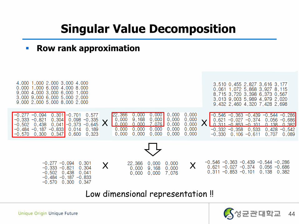
Singular Value Decomposition
Row rank approximation
X X
X X
Low dimensional representation !!
44
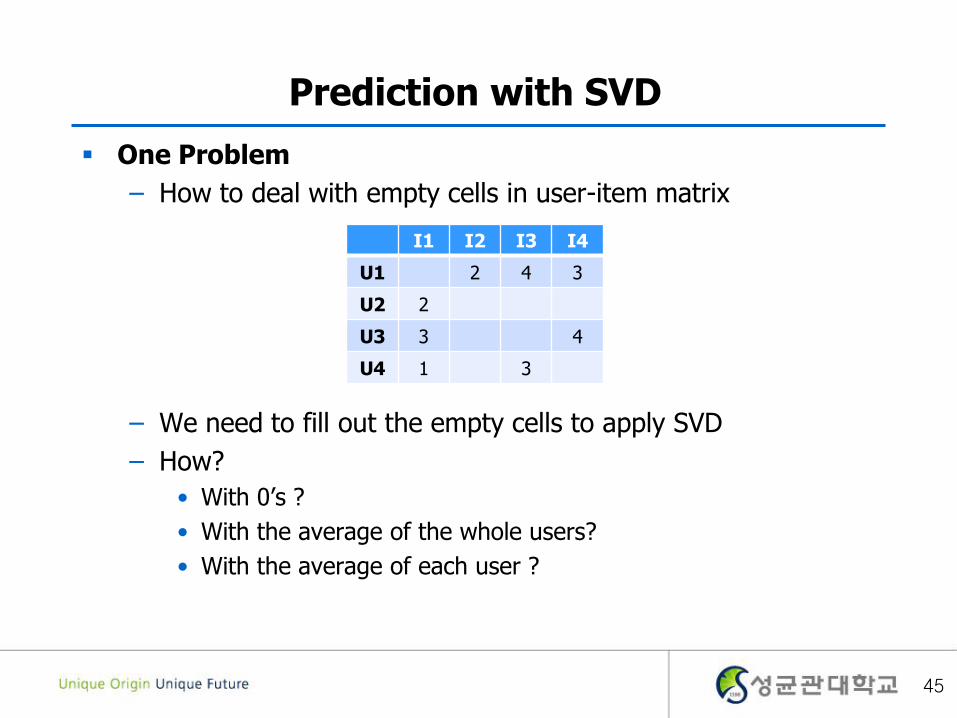
Prediction with SVD
One Problem
– How to deal with empty cells in user-item matrix
– We need to fill out the empty cells to apply SVD
– How?
• With 0’s ?
• With the average of the whole users?
• With the average of each user ?
I1 I2 I3 I4
U1 2 4 3
U2 2
U3 3 4
U4 1 3
45

Prediction with SVD
One Problem
– Considering both user bias and item bias
• There are users whose ratings are higher or lower than average
• Also, there are items of which ratings are higher or lower than average
– Example: Estimate John's rating of Titanic
• The average rating over all movies is 3.7 starts
• Titanic is rated 0.5 stars above the average movie
• John tends to rate 0.3 starts lower than the average
=>Titanic's rating by John would be (3.7+0.5-0.3)
46
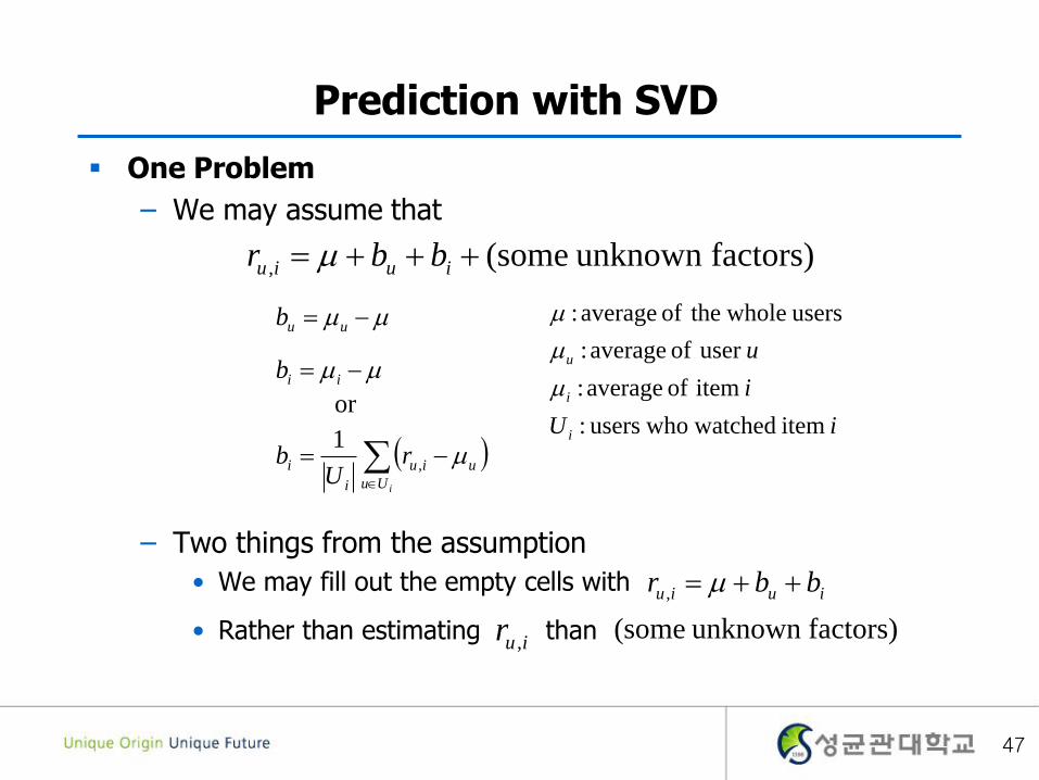
Prediction with SVD
One Problem
– We may assume that
– Two things from the assumption
• We may fill out the empty cells with
• Rather than estimating than
factors)unknown some(, iuiu bbr
uub
iUu
uiu
i
i rU
b ,
1iU
i
u
i
i
u
item watched whousers:
item of average :
user of average :
users whole theof average :
iib
or
iuiu bbr ,
iur ,factors)unknown some(
47

Prediction with SVD
Steps
– Normalizing rating matrix R
– Decompose R with SVD
– Reconstruct an approximated matrix
– De-normalizing the approximated matrix
48
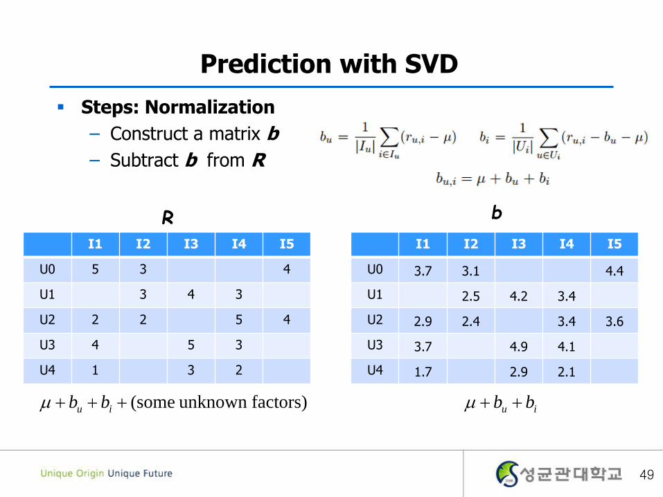
Prediction with SVD
Steps: Normalization
– Construct a matrix b
– Subtract b from R
I1 I2 I3 I4 I5
U0 5 3 4
U1 3 4 3
U2 2 2 5 4
U3 4 5 3
U4 1 3 2
I1 I2 I3 I4 I5
U0 3.7 3.1 4.4
U1 2.5 4.2 3.4
U2 2.9 2.4 3.4 3.6
U3 3.7 4.9 4.1
U4 1.7 2.9 2.1
bR
factors)unknown some( iu bb iu bb
49

Prediction with SVD
Steps: Low rank approximation
– Fill out empty cells with 0
– Decompose and approximate R-b with SVD
I1 I2 I3 I4 I5
U0 1.3 -0.1 0.0 0.0 -0.4
U1 0.0 0.5 -0.2 -0.4 0.0
U2 -0.9 -0.4 0.0 1.6 0.4
U3 0.3 0.0 0.1 -1.1 0.0
U4 -0.7 0.0 0.1 -0.1 0.0
R-b (unknown factors)I1 I2 I3 I4 I5
U0 1.3 -0.1 0.0 0.0 -0.3
U1 0.0 0.1 0.0 -0.5 0.0
U2 -0.9 -0.4 0.0 1.6 0.3
U3 0.3 0.2 0.0 -1.0 -0.1
U4 -0.7 0.1 0.0 -0.1 0.2
Approximation
factors)unknown some( factors)unknown some( of Estimation
50
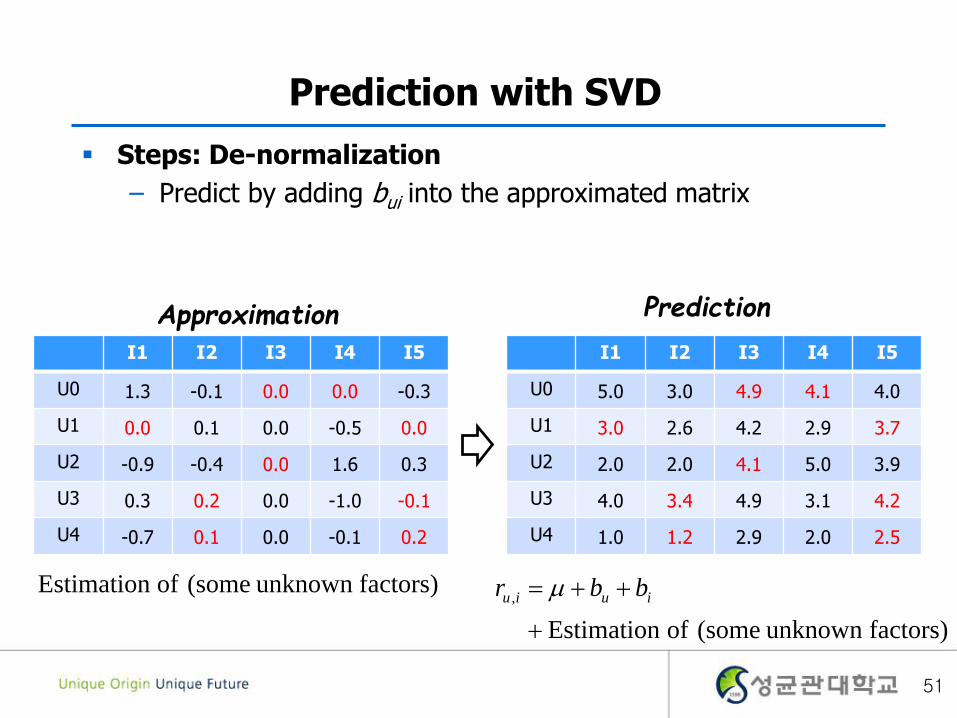
Prediction with SVD
Steps: De-normalization
– Predict by adding bui into the approximated matrix
I1 I2 I3 I4 I5
U0 1.3 -0.1 0.0 0.0 -0.3
U1 0.0 0.1 0.0 -0.5 0.0
U2 -0.9 -0.4 0.0 1.6 0.3
U3 0.3 0.2 0.0 -1.0 -0.1
U4 -0.7 0.1 0.0 -0.1 0.2
ApproximationI1 I2 I3 I4 I5
U0 5.0 3.0 4.9 4.1 4.0
U1 3.0 2.6 4.2 2.9 3.7
U2 2.0 2.0 4.1 5.0 3.9
U3 4.0 3.4 4.9 3.1 4.2
U4 1.0 1.2 2.9 2.0 2.5
Prediction
factors)unknown some( of Estimation
,
iuiu bbr factors)unknown some( of Estimation
51

Matrix Factorization through Optimization
For given , we want to find such that
NPPMNMNMNM VURRR where
NMR NPPM VU ,
R R’ UV
=x
52
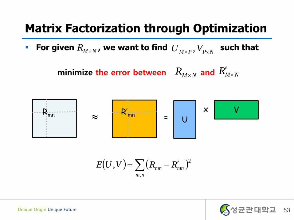
Matrix Factorization through Optimization
For given , we want to find such thatNMR NPPM VU ,
minimize the error between and NMR
NMR
nm
mnmn RRVUE,
2,
Rmn R’mnU
V=
x
53

Matrix Factorization through Optimization
For given ,
we want to find as simple as possible
NMR
NPPM VU ,
such that minimize the error between and NMR
NMR
np
pn
pm
mp
nm
mnmn VURRVUE,
2
,
2
,
2,
UV
=x
Rmn R’mn
54
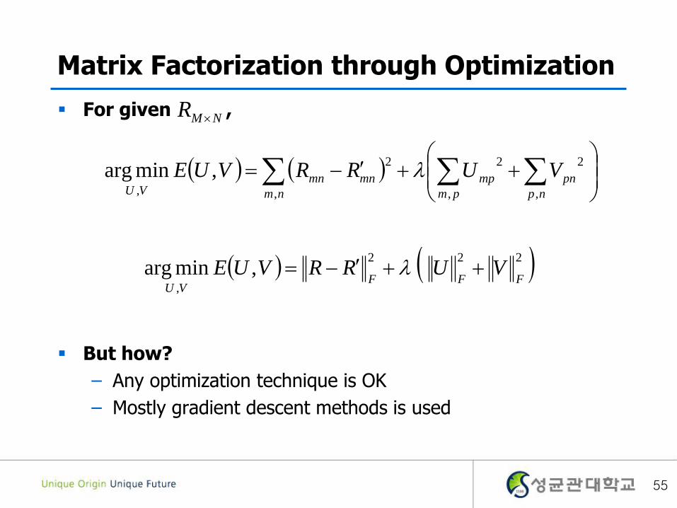
Matrix Factorization through Optimization
For given ,
But how?
– Any optimization technique is OK
– Mostly gradient descent methods is used
NMR
np
pn
pm
mp
nm
mnmnVU
VURRVUE,
2
,
2
,
2
,
,minarg
222
,
,minargFFF
VU
VURRVUE
55
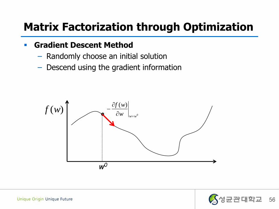
Matrix Factorization through Optimization
Gradient Descent Method
– Randomly choose an initial solution
– Descend using the gradient information
)(wf
w0
0
)(
www
wf
56

Matrix Factorization through Optimization
)(wf
w0 w1 w2 w3 w4
Moving Direction of w
Gradient Descent Method
– Randomly choose an initial solution
– Descend using the gradient information
57
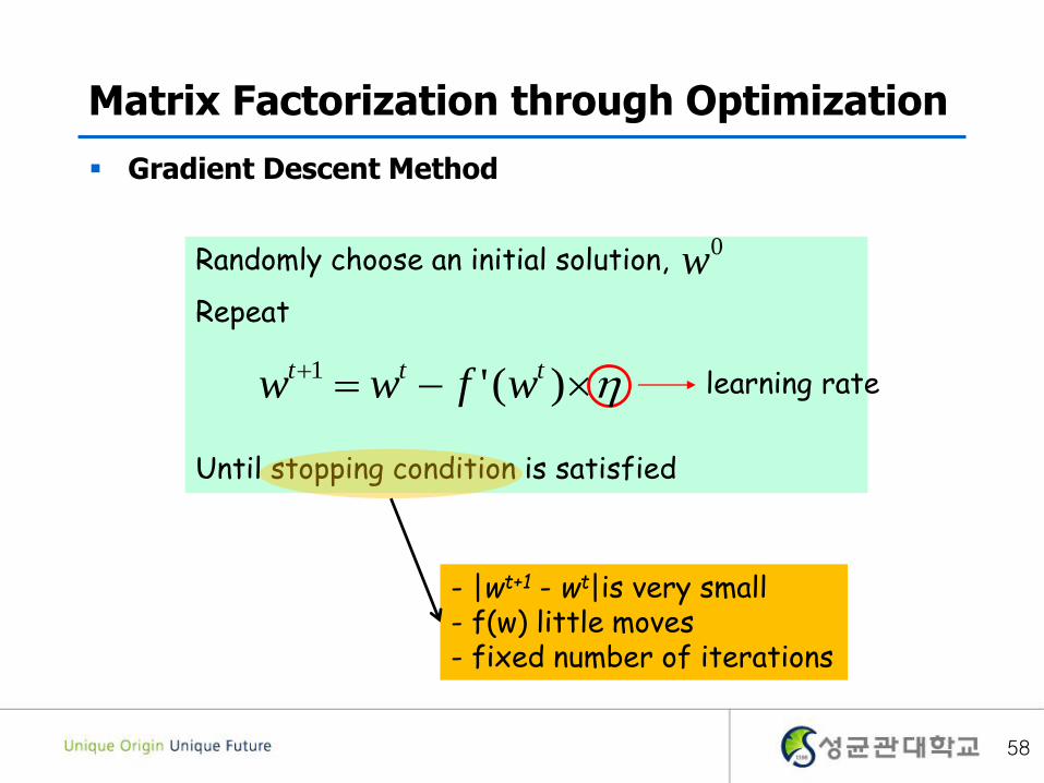
Matrix Factorization through Optimization
Gradient Descent Method
Randomly choose an initial solution,
Repeat
Until stopping condition is satisfied
learning rate )('1 ttt wfww
0w
- |wt+1 - wt|is very small- f(w) little moves - fixed number of iterations
58
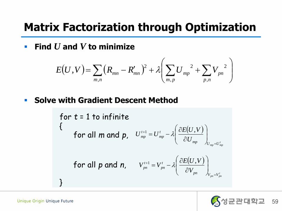
Find U and V to minimize
Solve with Gradient Descent Method
Matrix Factorization through Optimization
np
pn
pm
mp
nm
mnmn VURRVUE,
2
,
2
,
2,
tmpmp UUmp
t
mp
t
mpU
VUEUU
,1
tpnpn VVpn
t
pn
t
pnV
VUEVV
,1
for t = 1 to infinite {
}
for all m and p,
for all p and n,
59
Matrix Factorization through Optimization
Advantage
– Very flexible
– Easy to parallelize the optimization process (with GPUs)
– Easy to combine with other factors
60

Matrix Factorization through Optimization
Prediction
– Find U and V approximating R
– Find P and Q approximating the following
– Find everything except approximating the following
iuiu vur ,
iuiuiu qpbbr ,
iuiuiu qpbbr ,
61
Matrix Factorization through Optimization
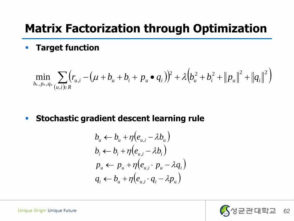
Target function
Stochastic gradient descent learning rule
Riu
iuiuiuiuiuqpb
qpbbqpbbr,
22222
,,, ***
min
uiiuui
iuiuuu
iiuii
uiuuu
pqebq
qpepp
bebb
bebb
,
,
,
,
62
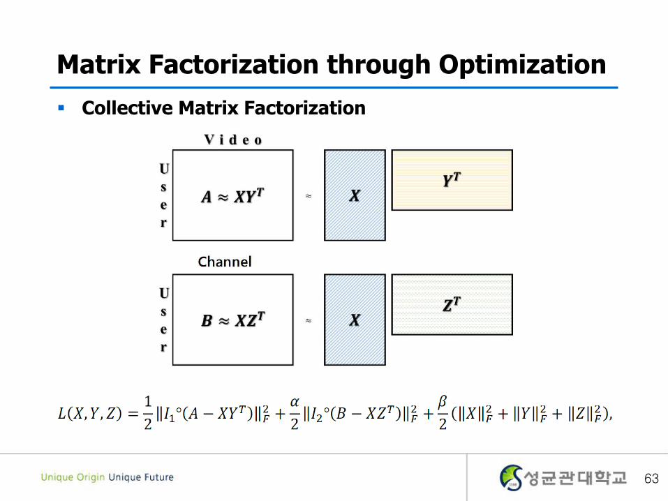
Matrix Factorization through Optimization
Collective Matrix Factorization
63

Summary of CF
Pros
– Requires minimal knowledge engineering efforts
– No need of any internal structure or characteristics
Cons
– Requires a large number of reliable ratings
– Assumes that prior behavior determines current behavior
– Cold start problems: New user, new items
– Sparsity problems
64

Outline
1. Introduction
2. Collaborative Filtering Overview
3. Memory based Collaborative Filtering
4. Model based Collaborative Filtering
5. Content based Recommender System
5-1. Overview
5-2. Vector Model
5-3. tf-idf weighting
5-4. Similarity between Documents
5-5. Advantage and Disadvantage
6. Summary
65

Overview
Contentmodeling
Similarcontent
Recommendation
ItemList
66
Overview
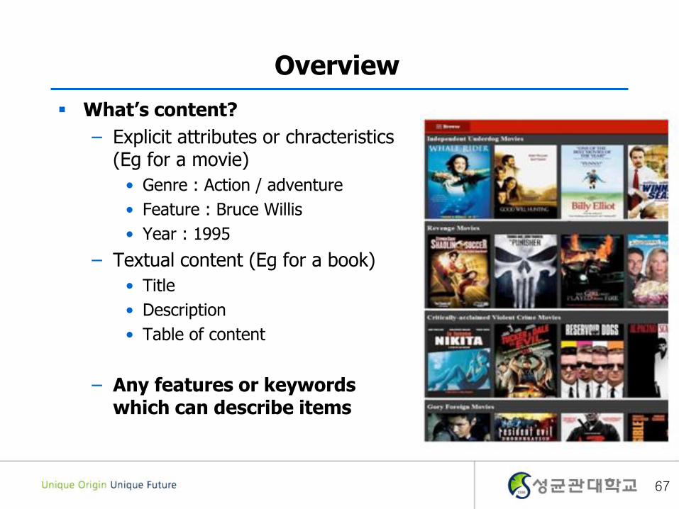
What’s content?
– Explicit attributes or chracteristics(Eg for a movie)
• Genre : Action / adventure
• Feature : Bruce Willis
• Year : 1995
– Textual content (Eg for a book)
• Title
• Description
• Table of content
– Any features or keywords which can describe items
67
Overview
Basic assumption and idea
– Customers will like similar content which they liked in the past
Suitable for text-based products (web pages, book)
– Items are “described” by their features (e.g. keywords)
– Users are described by the keywords in the items they bought
Characteristic
– Easy to apply to text-based products or products with text description
– Based on match between the content (item keywords) and user keywords
– Many machine learning approaches are applicable
• Neural Networks, Naive Bayesian, Decision Tree, …
68
Overview
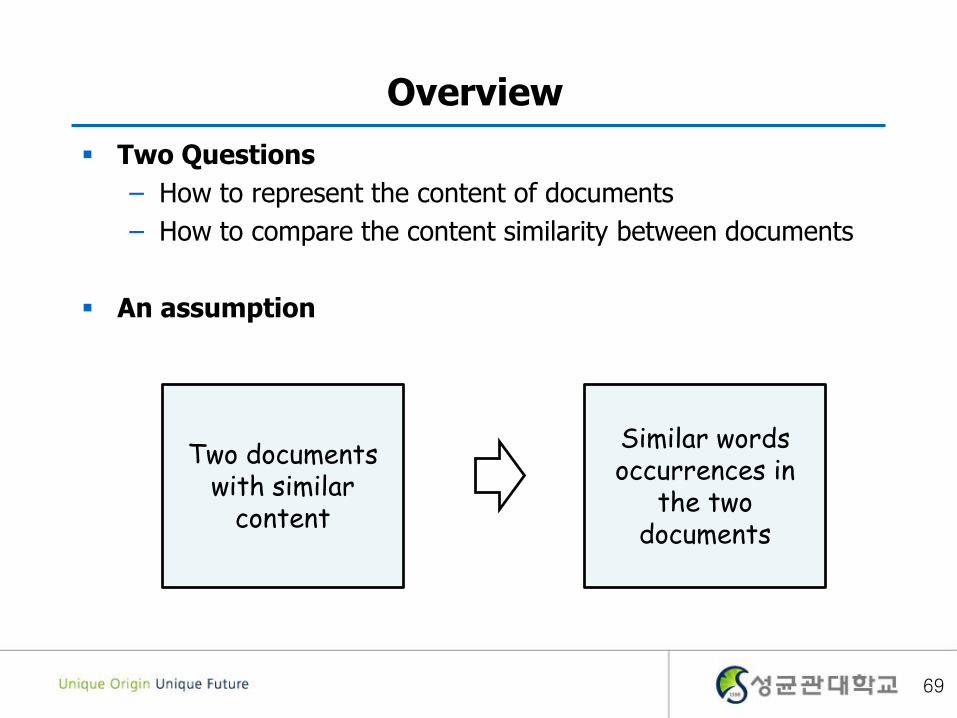
Two Questions
– How to represent the content of documents
– How to compare the content similarity between documents
An assumption
Two documents with similar
content
Similar words occurrences in
the two documents
69
Vector Model
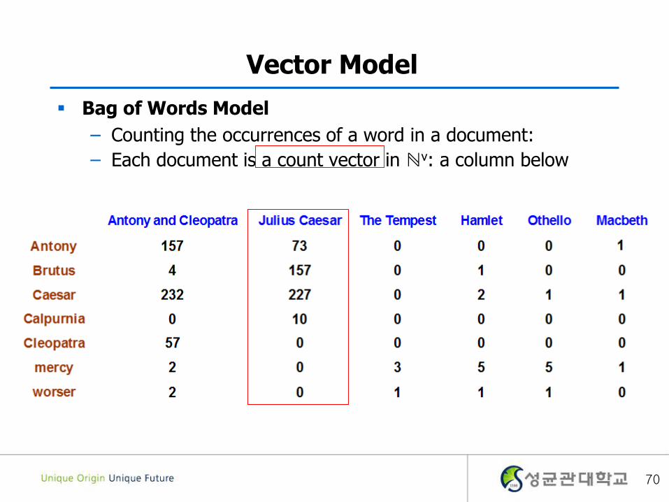
Bag of Words Model
– Counting the occurrences of a word in a document:
– Each document is a count vector in ℕv: a column below
70

Vector Model
Term Frequency Vector
– More frequent terms are more relevant to the content of the document
– But, it does not increase proportionally with term frequency
dtdtdtdt Nd ,,,, tf,,tf,tf,tf
321
documents ofset in the wordsdifferent ofnumber the:
in wordoffrequency term:tf ,
N
dtdw
71

Vector Model
Log-frequency weighting
otherwise 0,
0 tfif, tflog 1
10 t,dt,d
t,dw
tf 0 1 2 10 1000
w 0 1 1.3 2 4
72

Vector Model
But frequent words may be less informative
– Usually “a”, “the”, “is”, etc. have high term frequencies
– They are NOT so relevant to any content
Some less frequent words are more informative
Which words are important?
– Words frequent in the document, but infrequent in the document collection
– It is very probable that such words are strongly relevant to the content of the document
73
Vector Model
Term Frequency
– Represents how frequent a word in a document
Document Frequency (dft)
– Represents how frequent a word t in a document collection
– Defined as the number of documents that contain the word
– Higher Document Frequency -> Less Informative
– Lower Document Frequency -> More Informative
74

Vector Model
Inverse Document Frequency (idft)
term dft idft
calpurnia 1 6
animal 100 4
sunday 1,000 3
fly 10,000 2
under 100,000 1
the 1,000,000 0
t
t
N
df log idf 10
collection in the documents ofnumber the
wordcontaining documents ofnumber the df
N
tt
75
Vector Model
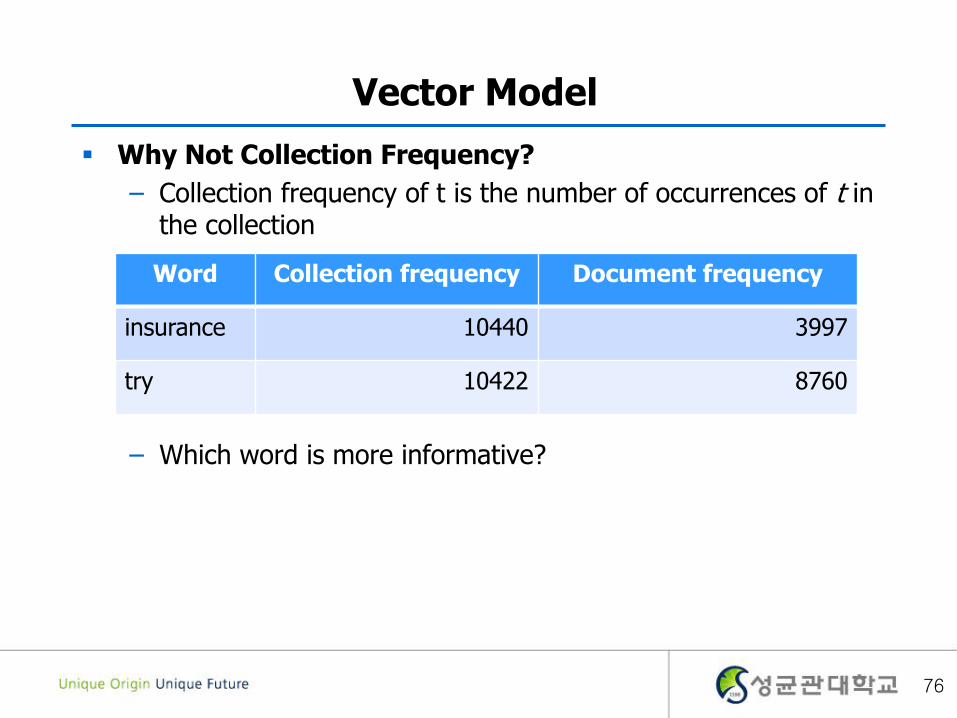
Why Not Collection Frequency?
– Collection frequency of t is the number of occurrences of t in the collection
– Which word is more informative?
Word Collection frequency Document frequency
insurance 10440 3997
try 10422 8760
76
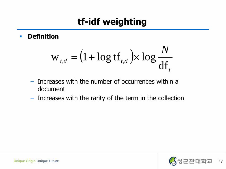
tf-idf weighting
Definition
– Increases with the number of occurrences within a document
– Increases with the rarity of the term in the collection
t
t,dt,d
N
dflogtflog1w
77
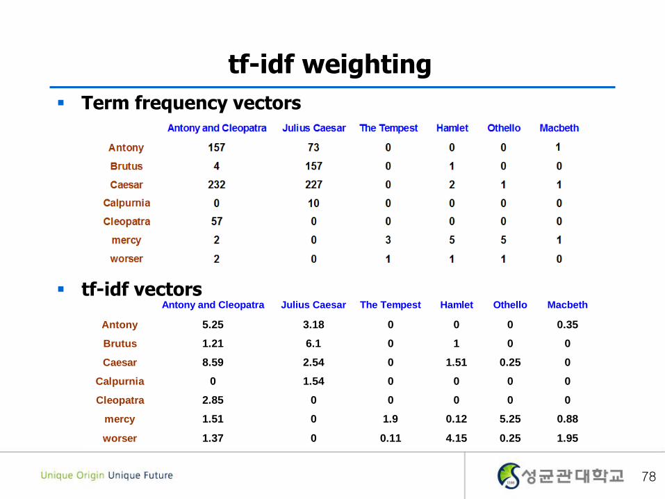
Antony and Cleopatra Julius Caesar The Tempest Hamlet Othello Macbeth
Antony 5.25 3.18 0 0 0 0.35
Brutus 1.21 6.1 0 1 0 0
Caesar 8.59 2.54 0 1.51 0.25 0
Calpurnia 0 1.54 0 0 0 0
Cleopatra 2.85 0 0 0 0 0
mercy 1.51 0 1.9 0.12 5.25 0.88
worser 1.37 0 0.11 4.15 0.25 1.95
tf-idf weighting
Term frequency vectors
tf-idf vectors
78

tf-idf weighting
So we have a |V|-dimensional vector space
– Terms are axes of the space
– Documents are points or vectors in this space
– Very high-dimensional and very sparse vectors
79
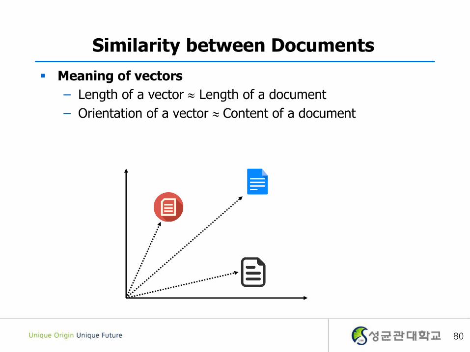
Similarity between Documents
Meaning of vectors
– Length of a vector Length of a document
– Orientation of a vector Content of a document
80

Similarity between Documents
Similarity
– Angle between two vectors is close to 0o
-> two documents have very similar content
– Angle between two vectors is close to 90o
-> two documents have irrelevant content each other
Angle from 0o
to 90o
– Similarity 1 to 0
– Cosine of the angle from 1 to 0
81
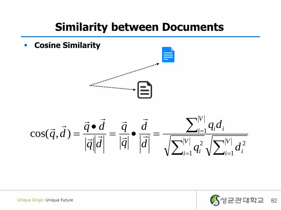
Similarity between Documents
Cosine Similarity
V
i i
V
i i
V
i ii
dq
dq
d
d
q
q
dq
dqdq
1
2
1
2
1),cos(
82
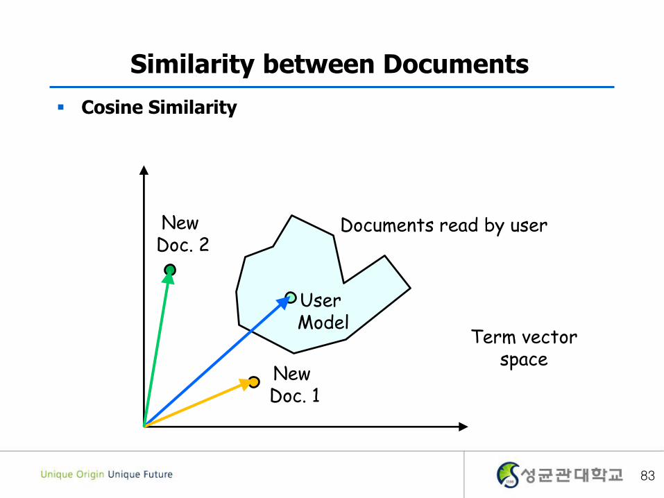
Similarity between Documents
Cosine Similarity
Documents read by user
User Model
New Doc. 1
New Doc. 2
Term vectorspace
83

Advantages of CBR
No need for data on other users
– No first-rater problem or sparsity problems
– Able to recommend new and unpopular items
Able to recommend to users with unique preference
Can provide explanations why it is recommended
– by listing content-features that caused an item to be recommended
Good to dynamically created items
– News, email, events, etc.
84
Disadvantages of CBR
Not easy to create content model for any products
– Book, web pages, news articles, music, video
Over-specialization
– Users are recommended with items similar to what they watched
– No serendipity
85

Outline
1. Introduction
2. Collaborative Filtering Overview
3. Memory based Collaborative Filtering
4. Model based Collaborative Filtering
5. Content based Recommender System
6. Summary
86
Summary
Recommendation
– Collaborative Filtering
– User-based Collaborative Filtering
– Item-based Collaborative Filtering
– Model-based Collaborative Filtering
– Content based Recommender System
RS are fairly new but already grounded on well-proven technology
However, there are still many open questions and a lot of interesting research to do
87

Thank you for your attention
Q&A
88
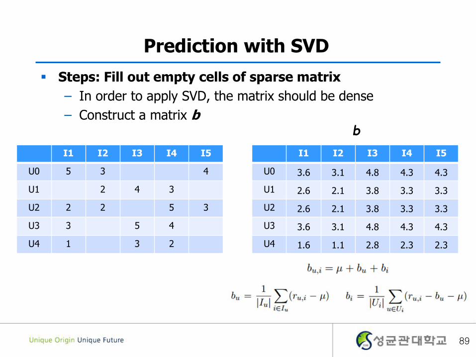
Prediction with SVD
Steps: Fill out empty cells of sparse matrix
– In order to apply SVD, the matrix should be dense
– Construct a matrix b
I1 I2 I3 I4 I5
U0 5 3 4
U1 2 4 3
U2 2 2 5 3
U3 3 5 4
U4 1 3 2
I1 I2 I3 I4 I5
U0 3.6 3.1 4.8 4.3 4.3
U1 2.6 2.1 3.8 3.3 3.3
U2 2.6 2.1 3.8 3.3 3.3
U3 3.6 3.1 4.8 4.3 4.3
U4 1.6 1.1 2.8 2.3 2.3
b
89
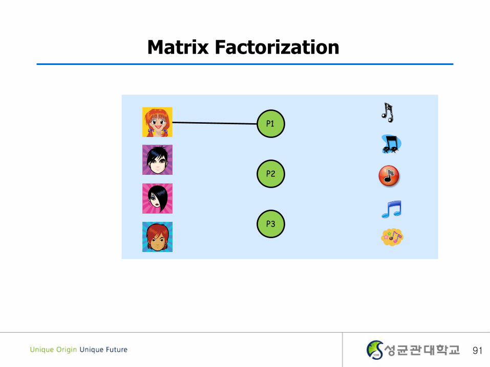
Matrix Factorization
P1
P2
P3
90
Matrix Factorization
P1
P2
P3
91

Matrix Factorization
P1
P2
P3
? ?
92


![An Adaptive Contextual Recommender System: a Slow ... · neighbor techniques [27, 21]. An important limitation of collaborative filtering systems is the cold start problem: situations](https://img.dokumen.tips/doc/110x75/5f8f3a0f89dccf16f71b2d2b/an-adaptive-contextual-recommender-system-a-slow-neighbor-techniques-27-21.jpg)


![[Final]collaborative filtering and recommender systems](https://img.dokumen.tips/doc/110x75/559c19c41a28ab18598b46f1/finalcollaborative-filtering-and-recommender-systems.jpg)