Embed Size (px)
Citation preview

Finlay et al. Earth, Planets and Space (2016) 68:112 DOI 10.1186/s40623-016-0486-1
FULL PAPER
Recent geomagnetic secular variation from Swarm and ground observatories as estimated in the CHAOS-6 geomagnetic field modelChristopher C. Finlay1* , Nils Olsen1, Stavros Kotsiaros1, Nicolas Gillet2 and Lars Tøffner‑Clausen1
Abstract
We use more than 2 years of magnetic data from the Swarm mission, and monthly means from 160 ground observa‑tories as available in March 2016, to update the CHAOS time‑dependent geomagnetic field model. The new model, CHAOS‑6, provides information on time variations of the core‑generated part of the Earth’s magnetic field between 1999.0 and 2016.5. We present details of the secular variation (SV) and secular acceleration (SA) from CHAOS‑6 at Earth’s surface and downward continued to the core surface. At Earth’s surface, we find evidence for positive accelera‑tion of the field intensity in 2015 over a broad area around longitude 90°E that is also seen at ground observatories such as Novosibirsk. At the core surface, we are able to map the SV up to at least degree 16. The radial field SA at the core surface in 2015 is found to be largest at low latitudes under the India–South‑East Asia region, under the region of northern South America, and at high northern latitudes under Alaska and Siberia. Surprisingly, there is also evidence for significant SA in the central Pacific region, for example near Hawaii where radial field SA is observed on either side of a jerk in 2014. On the other hand, little SV or SA has occurred over the past 17 years in the southern polar region. Inverting for a quasi‑geostrophic core flow that accounts for this SV, we obtain a prominent planetary‑scale, anti‑cyclonic, gyre centred on the Atlantic hemisphere. We also find oscillations of non‑axisymmetric, azimuthal, jets at low latitudes, for example close to 40°W, that may be responsible for localized SA oscillations. In addition to scalar data from Ørsted, CHAMP, SAC‑C and Swarm, and vector data from Ørsted, CHAMP and Swarm, CHAOS‑6 benefits from the inclusion of along‑track differences of scalar and vector field data from both CHAMP and the three Swarm satellites, as well as east–west differences between the lower pair of Swarm satellites, Alpha and Charlie. Moreover, ground observatory SV estimates are fit to a Huber‑weighted rms level of 3.1 nT/year for the eastward components and 3.8 and 3.7 nT/year for the vertical and southward components. We also present an update of the CHAOS high‑degree lithospheric field, making use of along‑track differences of CHAMP scalar and vector field data to produce a new static field model that agrees well with the MF7 field model out to degree 110.
Keywords: Geomagnetism, Secular variation, Field modelling, Core dynamics, Swarm
© 2016 The Author(s). This article is distributed under the terms of the Creative Commons Attribution 4.0 International License (http://creativecommons.org/licenses/by/4.0/), which permits unrestricted use, distribution, and reproduction in any medium, provided you give appropriate credit to the original author(s) and the source, provide a link to the Creative Commons license, and indicate if changes were made.
IntroductionThe Earth’s intrinsic magnetic field is gradually chang-ing as a result of motional induction and Ohmic dissipa-tion processes taking place within its metallic core. This
phenomenon, called geomagnetic secular variation (SV), has been well documented, but poorly understood, for centuries (e.g. Gellibrand 1635; Hansteen 1819). In 1980, MAGSAT provided the first truly global set of vector field observations. Combined with novel regularized inversion techniques, this enabled the structure of field at the core surface to be estimated for the first time with some con-fidence (Langel et al. 1980; Shure et al. 1982). Unfortu-nately, the MAGSAT mission lasted less than a year, so
Open Access
*Correspondence: [email protected] 1 Division of Geomagnetism, DTU Space, Technical University of Denmark, Diplomvej 371, Kongens Lyngby, DenmarkFull list of author information is available at the end of the article

Page 2 of 18Finlay et al. Earth, Planets and Space (2016) 68:112
inferences concerning SV were limited. It has only been in the past decade, thanks to the Ørsted and CHAMP missions, that it has become possible to map the large-scale patterns of the SV directly at the core surface (Lesur et al. 2008; Olsen et al. 2006). A picture has emerged of gradual (decadal) variations in SV punctuated by local-ized pulses of secular acceleration (SA) on shorter inter-annual timescales (Chulliat et al. 2010; Olsen et al. 2014). SA pulses provide an unexpected new window into the dynamics of the core, and we are still in the early stages of their study. We presently lack detailed knowledge of their morphology and their time dependence, and our understanding is severely limited by the relatively short time window for which there has been global monitoring from space.
A new opportunity for studying SV is today provided by the Swarm mission. Launched on 22 November 2013, it consists of three dedicated low-Earth-orbit satellites, each simultaneously measuring the near-Earth magnetic field. After more than 2 years of operation, Swarm data are starting to provide valuable new constraints on the time-varying SV. In this article, we present investigations of SV as observed by the Swarm satellites, and at ground observatories, in 2015 as part of a new time-dependent geomagnetic field model, called CHAOS-6, that also includes data from previous satellite missions (Ørsted, CHAMP, and SAC-C).
CHAOS-6 is the latest generation of the CHAOS series of global geomagnetic field models developed by Olsen et al. (2006, 2009, 2010, 2014). Ten months of Swarm data (up to September 2014) were included in the previous version, CHAOS-5 (Finlay et al. 2015), a model that was primarily designed for producing can-didate field models for IGRF-12. With more than 2 years of Swarm data now available, given there have been advances in the use of spatial differences (gradients) in field modelling (Kotsiaros et al. 2014; Olsen et al. 2015), and because a geomagnetic jerk happened in 2014 (Torta et al. 2015), there is now a clear need to update the CHAOS model series and particularly its time-dependent part, as CHAOS-6.
The CHAOS model series aims to estimate the inter-nal geomagnetic field at the Earth’s surface with high resolution in space and time. It is derived primarily from magnetic satellite data, although ground-based activity indices and observatory monthly means are also used. It includes a parameterization of the quiet-time, near-Earth magnetospheric field, but there is no explicit representation of the ionospheric field or fields due to magnetosphere–ionosphere coupling currents. A limi-tation of the CHAOS models series is that its validity is restricted to after 1999, when the Ørsted satellite was launched.
Other models with continuous time dependence are available for studying core field variations on longer time-scales, although these typically have lower resolution in both space and time. The gufm1 model (Jackson et al. 2000) is the definitive source for the historical field from 1590 to 1990. A more recent alternative spanning 1840 to 2010 is the COV-OBS model (Gillet et al. 2013) [see also Gillet et al. (2015a) for a version updated to 2015]. These models contain only a small amount of satellite data and are predominantly constrained by observatory data during the twentieth and twenty-first centuries. A rather different approach to modelling the recent field is provided by the comprehensive model series (Sabaka et al. 2004, 2015). The latest versions CM4 and CM5 cover 1960–2002 and 2000–2013, respectively, and involve simultaneous estimation of fields from a large number of sources including quiet-time ionospheric currents and magnetosphere–ionosphere coupling currents. This requires a much larger number of free parameters than is the case in the CHAOS models. A series of models of similar complexity to the CHAOS model, but derived only from CHAMP and ground obser-vatory data, is the GRIMM series of models (Lesur et al. 2008, 2010, 2015). The latter study is particularly interest-ing because it proposed field models with time depend-ence controlled by co-estimated core flows.
The main purpose of this article is to present CHAOS-6, providing a reference for users regarding its construc-tion. In the “Data” section, we detail the input data, while the model parameterization and estimation scheme are described in the “Field modelling” section. Model results and related discussion are presented in the “Results and discussion” section, including the fit to Swarm and CHAMP satellite data as well as ground observatory SV in the sections “Fit to satellite data” and “Fit to secular variation estimates from ground observatories” , respec-tively. The field and SV at Earth’s surface are described in the sections “Power spectra of field, SV and SA at Earth’s surface” and “Time changes in magnetic inten-sity at Earth’s surface” . The lithospheric field part of CHAOS-6 is described in the section “CHAOS-6h and the high-degree lithospheric field”. The field, SV and SA at the core surface are described in the section “Secular variation and acceleration at Earth’s core surface”. In the section “An interpretation based on quasi-geostrophic core flows”, we present for epoch 2015.0 a quasi-geos-trophic flow derived from the CHAOS-6 time-dependent field and SV. A summary and perspectives are offered in the “Conclusions” section.
DataThe database of magnetic observations used to con-struct CHAOS-6 is essentially an extension of that used by Finlay et al. (2015) to construct the CHAOS-5 model

Page 3 of 18Finlay et al. Earth, Planets and Space (2016) 68:112
in September 2014. The ground observatory vector field data have been updated as available in March 2016 (see the section “Ground observatory data”), while vector and scalar field data from the Swarm constellation up to 30 March 2016 have been included. The data selection cri-teria for satellite data at high latitudes have also been slightly altered compared with previous versions of the CHAOS model; further details are given in the “Satellite data” section.
A major improvement compared with CHAOS-5 is the inclusion of field spatial differences (i.e. approximate gradients) as data, along-track for both CHAMP and Swarm Alpha, Bravo and Charlie, and also east–west between Swarm’s lower satellite pair Alpha and Charlie. Along-track field differences approximate north–south gradients in non-polar regions (Kotsiaros et al. 2014; Sabaka et al. 2015), while the east–west differences pro-vide information on the longitudinal gradient of the field (Olsen et al. 2015). We constructed along-track field dif-ferences from data points from the same satellite track, separated by 15 s. East–west difference data were found by searching Swarm L1b 1 Hz magnetic data for a datum from Swarm Charlie, with latitude closest to a selected Swarm Alpha datum, within a maximum time difference of 50 s. This procedure typically resulted in time shifts of about 10 s between the contributing Alpha and Charlie data.
Ground observatory dataAnnual differences of revised observatory monthly means (Olsen et al. 2014) between January 1997 and December 2015 provide crucial constraints on the SV at fixed points on the Earth’s surface. Revised monthly means were derived from the hourly mean values of 160 observatories (for locations and IAGA codes see Fig. 1) that have been quality controlled, checking for trends, spikes and other errors (Macmillan and Olsen 2013). Quasi-definitive data (Peltier and Chulliat 2010; Clarke et al. 2013) were used when possible, for times when definitive data were not yet available; these quasi-definitive data are vital for deter-mining up-to-date secular variation and for comparisons with the latest data from the Swarm mission. Starting from hourly mean values, estimates of the ionospheric (plus induced) field from the CM4 model (Sabaka et al. 2004) and the large-scale magnetospheric (plus induced) field from a preliminary CHAOS-type model, CHAOS-6pre, were subtracted. Then a Huber-weighted monthly mean, including all local times and all disturbance levels, is computed. Taking annual differences, this procedure resulted in 23,466 vector field triples of SV estimates.
Satellite dataThe basic Ørsted, CHAMP and SAC-C dataset, sam-pled at a rate of 1 datum per 60 s, is the same as that employed in the earlier CHAOS-4 (Olsen et al. 2014) and
Fig. 1 Locations of ground magnetic observatories whose data are used in the derivation of CHAOS‑6. IAGA codes for the observatories are AAA, AAE, ABG, ABK, AIA, ALE, AMS, AMT, API, AQU, ARS, ASC, ASP, BDV, BEL, BFE, BFO, BGY, BJN, BLC, BMT, BNG, BOU, BOX, BRW, BSL, CBB, CBI, CDP, CKI, CLF, CMO, CNB, CSY, CTA, CZT, DLR, DLT, DMC, DOB, DRV, DVS, EBR, ELT, ESA, ESK, EYR, FCC, FRD, FRN, FUR, GAN, GDH, GLM, GNA, GNG, GUA, GUI, GZH, HAD, HBK, HER, HLP, HON, HRB, HRN, HTY, HUA, HYB, IPM, IQA, IRT, IZN, JCO, KAK, KDU, KEP, KHB, KIR, KIV, KMH, KNY, KNZ, KOU, KSH, KSH, LER, LIV, LMM, LNP, LOV, LRM, LRV, LVV, LYC, LZH, MAB, MAW, MBO, MCQ, MEA, MIZ, MMB, MOS, MZL, NAQ, NCK, NEW, NGK, NMP, NUR, NVS, OTT, PAF, PAG, PBQ, PET, PHU, PND, PST, QGZ, QIX, QSB, QZH, RES, SBA, SBL, SFS, SHU, SIL, SIT, SJG, SOD, SPT, SSH, STJ, SUA, TAM, TAN, TDC, TEO, TFS, THJ, THL, THY, TIR, TND, TRO, TRW, TSU, TUC, UPS, VAL, VIC, VSK, VSS, WHN, WIK, WNG, YAK, YKC

Page 4 of 18Finlay et al. Earth, Planets and Space (2016) 68:112
CHAOS-5 (Finlay et al. 2015) models. One difference compared with previous models is that CHAMP vector data were used only when attitude information from both star cameras was available.
Regarding the Swarm data, we used the Swarm Level-1b data product Mag-L, taking the latest available base-line 0408/09 data files in March 2016, for more than 28 months from 26 November 2013 to 30 March 2016. During this time, Swarm Alpha and Charlie descended from 514 to 445 km altitude, and Swarm Bravo, after being pushed up to 531 km altitude, has descended to 503 km. The local time of the ascending node of the three Swarm satellites has passed through more than two-and-a half 24-hour cycles, and Swarm Bravo is now separated from Swarm Alpha and Charlie by about 3 h of local time. The nominal 1 Hz data were sub-sampled at 60-s intervals unless no vector field magnetometer (VFM) or star tracker (STR) data were available. In addition, we rejected known disturbed days (for example when satel-lite manoeuvres occurred) and excluded gross outliers for which the vector field components were more than 500 nT (and the scalar field more than 100 nT) from the pre-dictions of a preliminary field model, CHAOS-6pre. In contrast to the case for CHAOS-5, no rescaling of Swarm vector data was necessary to ensure compatibility with the scalar data (Lesur et al. 2015), since the L1b baseline 0408/09 data calibration includes a co-estimated sun-driven disturbance that reduces rms scalar differences between the ASM and VFM measurements to under 200 pT (Tøffner-Clausen et al. 2016). After November 2014, calibration of the vector magnetometer on Swarm Char-lie has been carried out using scalar field values mapped over from Swarm Alpha; this is necessary due to total failure of the absolute scalar magnetometers on Swarm Charlie.
Following experience with the Swarm Initial Field Model (SIFM, see Olsen et al. 2015) and in preliminary experiments for CHAOS-6, we use different selection cri-teria for different classes of data:
For vector field data, we adopt the same quiet-time, dark, selection criteria that were used for earlier ver-sions of the CHAOS model series, namely (1) sun at least 10◦ below the horizon, (2) strength of the field due to the magnetospheric ring current, estimated using the RC index (Olsen et al. 2014), was required to change by at most 2 nT/h, (3) it was required that the geomagnetic activity index Kp ≤ 20 for quasi-dipole (Richmond 1995) latitudes equatorward of ±55◦.
As for earlier versions of the CHAOS model series, only scalar intensity data were used poleward of ±55◦ quasi-dipole latitude, and these were selected only when the merging electric field at the magnetopause (averaged over the preceding hour) Em ≤ 0.8 mV/m. In CHAOS-6,
Em was calculated using 1-min values of the interplan-etary magnetic field (IMF) and solar wind speed from OMNIWeb (http://omniweb.gsfc.nasa.gov), in contrast to earlier versions of the CHAOS model where 5-min mean values were used. In addition, an additional selection cri-terion that IMF BZ > 0 was introduced in CHAOS-6, motivated by a desire to avoid as far as possible distur-bances related to the sub-storm auroral electrojet that are especially prominent when IMF BZ < 0. Scalar data were also used at lower latitudes when attitude data were not available.
In CHAOS-6, we also make use of along-track and east–west differences of scalar data. As for the Swarm Initial Field model, SIFM (Olsen et al. 2015), scalar field differences were used at all latitudes and for all local times (including sunlit conditions, but excluding day-side equatorial region <±10◦ quasi-dipole latitudes), with slightly relaxed quiet-time criteria (RC index required to change by at most 3 nT/h and Kp ≤ 30). The same selec-tion criteria as for scalar data regarding Em and IMF BZ were applied to scalar field differences at polar latitudes. Scalar data have the advantage of not being directly per-turbed by the field-aligned currents that are a major con-tribution to the unmodelled external fields, particularly at polar latitudes. Olsen et al. (2015) found that includ-ing spatial differences of scalar data helped to improve the quality of both lithospheric field and secular variation models.
Along-track differences of vector data from the single satellite mission CHAMP and both along-track and east–west vector differences from the Swarm mission were also employed. For the vector field differences, we used the same selection criteria as for the vector data itself i.e. only data from dark (sun at least 10◦ below the horizon), non-polar (equatorward of ±55◦ quasi-dipole latitude) regions when the RC index changed by at most 2 nT/h and Kp ≤ 20 were selected.
For the low-degree part of CHAOS-6, called CHAOS-6l, 3 × 920,871 vector data, 942,303 scalar data, 1,793,294 along-track scalar differences, 424,003 east–west scalar differences, 3 × 403,382 along-track vector differences and 3 × 92,842 east–west vector differences were used. The reason for the much larger number of scalar differ-ences, compared with the number of scalar data, is that scalar differences were included for all local times (not just dark regions) and because their quiet-time selec-tion criteria were less strict. As in previous versions of the CHAOS model, all satellite data were also weighted proportional to sin θ, where θ is geographic co-latitude, in order to simulate an equal-area distribution.
Although iteratively reweighting of the data is per-formed during the model estimation (to implement a robust measure of misfit based on a Huber distribution of

Page 5 of 18Finlay et al. Earth, Planets and Space (2016) 68:112
errors, see the section “Field modelling”), we also employed an a priori error budget to account for the dif-ferences between the satellites. Regarding the scalar field, we assumed an a prior error estimate of 2.5 nT for Ørsted, CHAMP and SAC-C and 2.2 nT for Swarm. An isotropic pointing error estimate of 5 arc seconds was assumed for Swarm, 10 arc seconds for CHAMP (when both star cam-eras are available) and an anisotropic pointing error of 10 arc seconds and, respectively, 40 (60) arc seconds for after (before) 22 January 2000 for Ørsted. Note that these error estimates include the expected impact of unmodelled fields, which often dominate over instrumental errors.
Field modellingModel parameterizationThe model parameterization for CHAOS-6 follows closely that of CHAOS-5 and CHAOS-4. Since the focus of this article is the time-dependent internal field, we explicitly describe only this part of the model. See Olsen et al. (2014) for a more detailed account of the CHAOS field modelling scheme, including the external model. The time-dependent internal field Bint(t) = −∇V int(t) is represented as the gradient of the scalar potential
where a = 6371.2 km is a reference radius, (r, θ ,φ) are geographic coordinates and Pm
n (cos θ) are the Schmidt semi-normalized associated Legendre functions of degree n and order m. Note that we follow the usual geomagnetic convention and refer to B as the magnetic field, though it is strictly the magnetic flux density. In the vacuum, it is related to the magnetic field H by B = µ0H where µ0 is the permeability of free space.{
gmn (t), hmn (t)}
are time-dependent Gauss coeffi-cients that are further expanded in a basis of sixth-order B-splines (De Boor 2001) such that
and similarly for hmn (t), where kgmn are the spline coeffi-cients estimated for each Gauss coefficient, K = 6 (sixth-order B-splines), Bk are the spline basis functions, and we use a 6-month knot spacing with fivefold repeated knots at the endpoints t = 1997.1 and t = 2016.6.
In addition to a time-dependent internal field, we also estimate a static internal field above degree 20. The low-degree part of CHAOS-6 model that is the focus of this section, CHAOS-6l, was estimated using a maximum
(1)
V int = a
20∑
n=1
n∑
m=0
[
gmn (t) cosmφ + hmn (t) sinmφ]
×
(a
r
)n+1
Pmn (cos θ)
(2)gmn (t) =
K∑
k=1
kgmn Bk(t),
degree of 80 (in contrast the high-degree part of the CHAOS-6 model, CHAOS-6h was estimated using a maximum degree of 120—see the section “CHAOS-6h: estimation of the high-degree lithospheric field”).
Regarding the external field, as in earlier CHAOS mod-els, we use a representation of fields due to near-Earth magnetospheric sources, e.g. the magnetospheric ring current, in the solar magnetic (SM) coordinate system (up to n = 2, with time dependence for n = 1 parameter-ized by the external and induced parts of the RC index) and of fields due to remote magnetospheric sources, e.g. magnetotail and magnetopause currents, in geocen-tric solar magnetospheric (GSM) coordinates (also up to n = 2, but restricted to order m = 0). Additional offset parameters in bins of width 5 days, respectively, 30 days are included for the degree 1 SM terms, for orders m = 0 , respectively m = 1.
We also co-estimate the Euler angles needed to describe the rotation between the vector magnetometer frame and the star imager frame. For Ørsted, this yields two sets of Euler angles (one for the period before 22 Jan-uary 2000 when the onboard software of the star imager was updated and one for the period after that date), while for CHAMP and each Swarm satellite we solve for Euler angles in bins of 10 days.
Model estimationModel parameters were estimated using an iteratively reweighted least-squares algorithm making use of Huber weights. Regularization of temporal variations was also included. Specifically, we minimized the cost function
where m is the model vector, C is the data error covari-ance matrix which includes anisotropic errors due to attitude uncertainty (Holme and Bloxham 1996) and �
3 and �
2 are block diagonal regularization matrices
penalizing the squared values of the third, respectively second, time derivatives of the radial field Br at the core surface. �
3 involves integration over the full time span
of the model, while �2 involves evaluating the second
time derivative only at the model endpoints t = 1997.1 and 2016.6. �3 and �2 determine the strength of the regularization applied to the model time dependence during the entire modelled interval and at the end-points, respectively. We tested several values for these parameters and finally selected �3 = 0.66 (nT/year3)−2, �2 = 100 (nT/year2)−2 for the start time t = 1997.1 and �2 = 300 (nT/year2)−2 for the end time t = 2016.6. All time-dependent zonal terms were treated separately with �3 set to a larger value of 60 (nT/year3)−2.
(3)eTC−1
e+ �3mT�
3m + �2m
T�2m

Page 6 of 18Finlay et al. Earth, Planets and Space (2016) 68:112
The vector of residuals e comprises differences between data and model predictions
It involves vector and scalar data, denoted by dobs, and the associated model predictions dmod = Gm, where G is the design matrix for the forward model. For sca-lar data, G is the forward operator linearized around the present model. The data in CHAOS-6 also include along-track and east–west vector and scalar field dif-ferences, denoted by �dobs = dobs(r2, t2)− dobs(r1, t1) . The associated model predictions are �dmod = �Gm = [G(r2, t2)−G(r1, t1)]m. Further details of the implementation of along-track and across-track differences in field modelling are described by Kot-siaros et al. (2014) and Olsen et al. (2015, 2016).
In deriving the CHAOS-6l time-dependent field model, we estimated 28,766 model parameters from 7,481,013 observations. The final model was obtained after 9 iterations.
CHAOS‑6h: estimation of the high‑degree lithospheric fieldThe final version of CHAOS-6 was obtained by taking the model coefficients from CHAOS-6l (as described above) and replacing the static field Gauss coefficients above degree n = 24 with the static field coefficients from the CHAOS-6h model, truncated at degree n = 110. CHAOS-6h is a new dedicated model of the high-degree lithospheric field. As for the CHAOS-4h model (Olsen et al. 2014), that provided the high-degree static field in both CHAOS-4 and CHAOS-5, it was derived only using low-altitude, solar minimum CHAMP data, from August 2008 to September 2010.
In addition to scalar and vector field data, CHAOS-6h makes use of along-track scalar and vector field differences from CHAMP. The data selection criteria for the vector and scalar field data are the same as for CHAOS-6l. However, for CHAOS-6h, identical selec-tion criteria are used for both scalar and vector field differences. Data are selected only if Kp ≤ 30, and |dDst/dt| ≤ 3 nT/h. Both night and dayside data are selected, excluding the dayside equatorial region (<±10◦ quasi-dipole latitudes). Regarding the CHAOS-6h model parameterization, a static field up to n = 120 was estimated, with a time-dependent internal field for n ≤ 16 described by a third-order Taylor expansion (quadratic SV). The same bin lengths as in CHAOS-6l were used for the RC baseline correction terms and for the instrument alignment calibration parameters (Euler angles). As for CHAOS-4h (Olsen et al. 2014), we applied regularization above degree n = 90 by mini-mizing the L2 norm of Br at Earth’s surface.
(4)e =
[
dobs
�dobs
]
−
[
dmod
�dmod.
]
.
In all, 15,636 model parameters were estimated from 3,306,074 CHAMP observations when deriving CHAOS-6h.
Results and discussionFit to satellite dataThe fit of the CHAOS-6l field model to scalar and vec-tor satellite data is generally similar (within 0.15 nT) to the fits achieved by CHAOS-5. For example, the Huber-weighted rms misfit between CHAOS-6l and non-polar scalar field data is 2.12 nT for CHAMP in comparison with 2.20nT, 2.18nT and 2.19nT, respectively, for Swarm Alpha, Beta and Charlie. The misfit to the Bφ vector com-ponent is 2.54 nT for CHAMP and 2.50, 2.47 and 2.50 nT, respectively, for Swarm Alpha, Beta and Charlie.
Field difference data were not included in earlier CHAOS models; CHAOS-6 is the first field model to be derived using along-track spatial differences of vector data from both CHAMP and Swarm. Figure 2 presents histograms of residuals for the vector field differences. Comparing Swarm along-track and east–west differ-ences, the along-track differences (involving measure-ments made on the same orbit by the same instrument) have Huber-weighted rms misfits of 0.27, 0.27 and 0.34 nT for the radial, north–south and east–west compo-nents, compared with 0.47, 0.50 and 0.57 nT for the east–west vector field differences between Swarm Alpha and Charlie. Despite involving measurements from different satellites, we conclude the east–west vector field differ-ences from Swarm are reliable and an internal field model is able to fit them to a weighted rms level of approxi-mately 0.5 nT. Of course no east–west differences were possible with CHAMP, but we can compare the along-track differences. We find Huber-weighted rms misfits of 0.36, 0.36 and 0.40 nT for along-track differences of the radial, north–south and east–west vector field com-ponents from CHAMP. The along-track differences of Swarm vector data thus have generally smaller residuals than similar differences constructed with CHAMP data. This augurs well for the future of the Swarm mission as the satellites descend.
Fit to secular variation estimates from ground observatoriesThe highest quality records of geomagnetic secular varia-tion and its time variability come from ground magnetic observatories, where absolute calibrations are routinely carried out. If we are to use CHAOS-6 (which is primar-ily determined by fitting satellite data) to study secu-lar variation, it is essential that it also fits the available ground observatory data well. We find Huber-weighted rms misfits of CHAOS-6 to annual differences of ground observatory revised monthly means of 3.80, 3.65 and 3.07

Page 7 of 18Finlay et al. Earth, Planets and Space (2016) 68:112
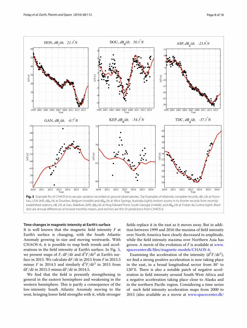
nT/year, respectively, for the radial, north–south and east–west components.Examples of ground observatory secular variation time series, along with CHAOS-6 model predictions, are pre-sented in Fig. 3. The top row shows examples of some complete series spanning 1999 to 2016 from well-estab-lished observatories at Honolulu (HON) in the central Pacific, at Dorbes (DOU) in Europe and at Alice Springs (ASP) in Australia. We find that CHAOS-6 provides a good description of the time-dependent SV in all these locations. There are noticeable sub-decadal changes in the SV trends even in the central Pacific where SV is often considered to be less intense. As pointed out by
Torta et al. (2015), a geomagnetic jerk (characterized by a ‘V’ shape in the SV as the SA changes sign) clearly occurred in 2014. This jerk event is generally well cap-tured by the CHAOS-6 model.
In addition to presenting examples from well-estab-lished observatories, Fig. 3 also shows shorter time series at three recently established observatories in remote locations, at Gan in the southern Maldives, at King Edward Point (KEP) in South Georgia and at Tristan da Cunha (TDC) in the mid-Atlantic. Note that these plots are zoomed in compared to the previous plots and they cover only the shorter time interval of 2010–2015. CHAOS-6 again satisfactorily fits the data from these newer observatories, even when sharp changes in SV are observed, for example in dBφ/dt at Tristan da Cunha in 2014. Although the fit to KEP in Fig. 3 is visually less impressive than that at TDC, note that it is for the north–south field component, while the (typically quieter) east–west component is presented for TDC. The rms weighted residuals for dBr/dt, dBθ /dt, dBφ/dt are, respectively, 1.2, 1.6, 0.9 nT/year for TDC and 1.65, 2.40, 2.09 nT/year for KEP.
Power spectra of field, SV and SA at Earth’s surface In Fig. 4, we present the Lowes–Mauersberger spheri-cal harmonic power spectra for the vector field, its first time derivative (SV) and its second time derivative (SA) at the Earth’s surface in 2015. The spectra for the field itself decreases steadily until approximately degree 14, after which it begins to level out. The change from a neg-ative (decreasing) slope to a positive (increasing) slope, which indicates that lithospheric sources are certainly dominating, does not take place until degree 18. At the Earth’s surface, the spectrum of the SV also decreases with degree; the slope begins to level out about degree 19, indicative of the noise floor being reached. In con-trast to the field and the SV, the SA spectra converges at the surface for CHAOS-6 in 2015, with essentially zero power remaining by its truncation degree 20. This is a consequence of the model regularization, that forces the SA towards zero at the model endpoints and minimizes time changes in the SA throughout, which is stronger at higher degree. The low values of the SA spectrum at high degrees should thus not be taken as indicative of a detection limit for the SA which would be related to the noise spectrum; the detection limit can only be prop-erly assessed in unregularized inversions. The SA power spectrum shows weak peaks at degrees 3, 5, 7 and 9 in 2015. Given the surface spectra are well behaved and not diverging, the entire time-dependent part of the CHAOS-6 model (up to spherical harmonic degree 20) can legitimately be used to map and investigate time-dependent secular variation at the Earth’s surface.
-2 -1.5 -1 -0.5 0 0.5 1 1.5 20
0.2
0.4
0.6
0.8
1
1.2
1.4
1.6
1.8
Misfit [nT]
pdf,
nor
mal
ised
dBr, σ=0.27nT
dBθ, σ=0.27nT
dBφ, σ=0.34nT
dBr EW, σ=0.47nT
dBθ EW, σ=0.50nT
dBφ EW, σ=0.57 nT
-2 -1.5 -1 -0.5 0 0.5 1 1.5 20
0.2
0.4
0.6
0.8
1
1.2
1.4
1.6
1.8
Misfit [nT]
pdf,
nor
mal
ised
dBr, σ=0.27nT
dBθ, σ=0.27nT
dBφ, σ=0.34nT
dBr CH, σ=0.36nT
dBθ CH, σ=0.36nT
dBφ CH, σ=0.40nT
Fig. 2 Histograms of satellite data residuals from CHAOS‑6l, for vector field spatial differences (gradients). Blue colours are radial com‑ponent differences, red/brown colours are north–south component differences, and green colours are east–west component differences. Top A comparison of Swarm along‑track and east–west differences residuals. Darker colours are the along‑track differences and brighter colours the east–west differences. Bottom A comparison of along‑track Swarm residuals (darker colours) and along‑track CHAMP residu‑als (brighter colours, with dots). The histograms have been normalized so that each has the same integrated area
Page 8 of 18Finlay et al. Earth, Planets and Space (2016) 68:112
Time changes in magnetic intensity at Earth’s surfaceIt is well known that the magnetic field intensity F at Earth’s surface is changing, with the South Atlantic Anomaly growing in size and moving westwards. With CHAOS-6, it is possible to map both trends and accel-erations in the field intensity at Earth’s surface. In Fig. 5, we present maps of F, dF/dt and d2F/dt2 at Earth’s sur-face in 2015. We calculate dF/dt in 2015 from F in 2015.5 minus F in 2014.5 and similarly d2F/dt2 in 2015 from dF/dt in 2015.5 minus dF/dt in 2014.5.
We find that the field is presently strengthening in general in the eastern hemisphere and weakening in the western hemisphere. This is partly a consequence of the low-intensity South Atlantic Anomaly moving to the west, bringing lower field strengths with it, while stronger
fields replace it in the east as it moves away. But in addi-tion between 1999 and 2016 the maxima of field intensity over North America have clearly decreased in amplitude, while the field intensity maxima over Northern Asia has grown. A movie of the evolution of F is available at www.spacecenter.dk/files/magnetic-models/CHAOS-6.
Examining the acceleration of the intensity (d2F/dt2 ), we find a strong positive acceleration is now taking place in the east, in a broad longitudinal sector from 30◦ to 120◦E. There is also a notable patch of negative accel-eration in field intensity around South-West Africa and a negative acceleration taking place close to Alaska and in the northern Pacific region. Considering a time series of such field intensity acceleration maps from 2000 to 2015 (also available as a movie at www.spacecenter.dk/
1999 2001 2003 2005 2007 2009 2011 2013 2015
0
10
20
30
40
50
60
HON, dBr/dt, 21.3°N
Year
[nT/yr]
1999 2001 2003 2005 2007 2009 2011 2013 2015
-6
-4
-2
0
2
4
6
8
DOU, dBθ/dt, 50.1°N
Year
[nT/yr]
1999 2001 2003 2005 2007 2009 2011 2013 2015
-30
-25
-20
-15
-10
-5
0
5
10
15
ASP,dBφ/dt, -23.8°N
Year
[nT/yr]
2010 2011 2012 2013 2014 2015 2016
-75
-70
-65
-60
-55
-50
-45
-40
-35
GAN, dBr/dt, -0.7°N
Year
[nT/yr]
2010 2011 2012 2013 2014 2015 2016
60
65
70
75
KEP,dBθ/dt, -54.3°N
Year
[nT/yr]
2010 2011 2012 2013 2014 2015 2016
24
26
28
30
32
34
36
38
40
42
TDC, dBφ/dt, -37.1°N
Year
[nT/yr]
Fig. 3 Example fits of CHAOS‑6 to secular variation recorded at ground observatories. Top Examples of relatively complete records, dBr/dt at Hono‑lulu, USA (left), dBθ /dt at Dourbes, Belgium (middle) and dBφ/dt at Alice Springs, Australia (right); bottom zooms in to shorter records from recently established stations, dBr/dt at Gan, Maldives (left), dBθ /dt at King Edward Point, South Georgia (middle), and dBφ/dt at Tristan da Cunha (right). Black dots are annual differences of revised monthly means, and red lines are the SV predictions from CHAOS‑6

Page 9 of 18Finlay et al. Earth, Planets and Space (2016) 68:112
files/magnetic-models/CHAOS-6), we find the intensity acceleration changes dramatically on sub-decadal time-scales. For example, a series of prominent oscillations are observed west of southern Africa. The field, the SV and the SA downward continued to the core surface are pre-sented later in the section “Secular variation and accel-eration at Earth’s core surface” and in Fig. 9.
In order to test the above inferences concerning field intensity changes made using the CHAOS-6 field model, in Fig. 6 we present time series of field intensity changes, based on annual differences of ground observatory revised monthly means (F is in this case calculated from the revised month values of Br, Bθ, Bφ). A positive inten-sity acceleration in 2015 is clearly seen at Novosibirsk, Russia, at eastern longitudes in the northern hemisphere and is also evident although weaker at Niemegk, Ger-many, and at Learmouth, Australia. A relatively long-term negative acceleration is evident in the rate of field intensity decrease observed in Alaska. Overall, we are satisfied that CHAOS-6 adequately explains the observed trends and accelerations of the recent geomagnetic field intensity.
CHAOS‑6h and the high‑degree lithospheric field Turning to the higher degree static field in CHAOS-6 (from CHAOS-6h, see the section “CHAOS-6h: estima-tion of the high-degree lithospheric field”), Fig. 7 presents a map of the lithospheric part of the radial field (degrees 15–110) along with the power spectrum and degree cor-relation at the Earth’s surface in comparison with MF7 (Maus 2010) and CHAOS-4. CHAOS-6 agrees with MF7 much better than CHAOS-4 whose power spectra begin to show deviations above degree 83, when the degree cor-relation also drops below 0.85. In contrast, the spectrum
for CHAOS-6 remains close to that of MF7 up to degree 110, and only after this, does its degree correlation fall below 0.85. We therefore consider the static field in CHAOS-6 to be reliable up degree 110 and recommend its use to this degree.
The map in Fig. 7 shows the radial field plotted at the Earth’s surface considering degrees 16 to 110. The map
0 1 2 3 4 5 6 7 8 9 10 11 12 13 14 15 16 17 18 19 2010-10
10-5
100
105
1010
degree n
Pow
er [n
T2 ] or [
(nT/
yr)2 ] o
r [(n
T/yr
2 )2 ]
Fig. 4 Lowes–Mauersberger spherical harmonic power spectra of the vector magnetic field (black), secular variation (red) and secular acceleration (blue) at the Earth’s surface in 2015
Fig. 5 Field intensity (top), its rate of change (middle) and its accelera‑tion (bottom) at Earth’s surface in 2015. Units are µT = 103nT, nT/year and nT/year2 , respectively. Map projection is Hammer‑Aitoff

Page 10 of 18Finlay et al. Earth, Planets and Space (2016) 68:112
displays well-localized anomalies, especially over the continents. Over the oceans, short-wavelength north–south linear features are visible, despite their relatively low amplitude. Differences to MF7 are mostly with respect to these features. Some differences, especially around auroral electrojet latitudes south of Australia, are possibly due to disturbed tracks, but it may also be that MF7 lacks some along-track power due to the filtering applied during its construction. It will be interesting to see how this part of the signal develops in future models constructed from Swarm data, as the lower pair of satel-lites descend and they are better able to resolve the short-wavelength east–west field gradients.
Statistics regarding the Huber-weighted mean and rms misfits of CHAOS-6h to the CHAMP field and field dif-ference data used to construct it are presented in Table 1.
Secular variation and acceleration at Earth’s core surfaceIn order to study the origin of secular variation, it is nec-essary to downward continue the field to the outer edge of its source region in the core. We carry out the down-ward continuation, assuming that there are no current sources in the mantle on the timescale of observable sec-ular variation, so the field continues to be described by a potential. The resulting spectra for the field, SV and SA at the core surface in 2015 are presented in Fig. 8.
Above degree 13, we see an upward trend in the field spectrum that we attribute to lithospheric sources. We therefore choose to present maps of the field at the core surface only to degree 13. The SV spectra increases rap-idly with degree at first, but levels out above degree 9. It starts to increase more rapidly again above degree 18; plotting maps of the SV at the core surface, we see this
1999 2001 2003 2005 2007 2009 2011 2013 2015-50
-40
-30
-20
-10
0
10
20
30
CMO, dF/dt, 64.9°N
Year
[nT/yr]
1999 2001 2003 2005 2007 2009 2011 2013 201525
30
35
40
NGK, dF/dt, 52.1°N
Year
[nT/yr]
1999 2001 2003 2005 2007 2009 2011 2013 2015
20
25
30
35
40
45
50NVS, dF/dt, 54.9°N
Year
[nT/yr]
1999 2001 2003 2005 2007 2009 2011 2013 2015-90
-85
-80
-75
-70
-65
-60
-55
KOU, dF/dt, 5.2°N
Year
[nT/yr]
1999 2001 2003 2005 2007 2009 2011 2013 2015-80
-75
-70
-65
-60
-55
-50
-45
-40
HER, dF/dt, -34.4°N
Year
[nT/yr]
1999 2001 2003 2005 2007 2009 2011 2013 2015
-45
-40
-35
-30
-25
-20
-15
-10
-5
0
LRM, dF/dt, -22.2°N
Year
[nT/yr]
Fig. 6 Fit of CHAOS‑6 to secular variation of intensity (dF/dt) at example ground observatories. Top College station, Alaska (left); Niemengk, Ger‑many (middle); and Novosibirsk, Russia (right); bottom Kourou, French Guiana (left); Hermanus, South Africa (middle); and Learmouth, Australia (right)

Page 11 of 18Finlay et al. Earth, Planets and Space (2016) 68:112
is associated with an increase in disorganized noise in maps. We therefore believe the SV in CHAOS-6 is satis-factory out at least to degree 16, and possibly even as far as degree 18. Turning to the SA spectrum, in CHAOS-6
this converges at high degree at the core surface due to the applied regularization. In 2015 (relatively close to the model endpoint), regularization starts to dominate the solution already above degree 9. We nonetheless choose
20 30 40 50 60 70 80 90 100 110 120
100
101
degree n
Rn [n
T2 ]
MF7CHAOS−6CHAOS−4CHAOS−6 − MF7CHAOS−4 − MF7CHAOS−4 − CHAOS−6
20 30 40 50 60 70 80 90 100 110 1200.7
0.75
0.8
0.85
0.9
0.95
1
degr
ee c
orre
latio
n ρ n
degree n
CHAOS−6 vs. MF7CHAOS−4 vs. MF7CHAOS−4 vs. CHAOS−6
Fig. 7 Top Map of the radial magnetic field at Earth’s surface for degrees 16–110 from CHAOS‑6, units: nT. Map projection is Hammer‑Aitoff. Bottom Spherical harmonic power spectra (left) and degree correlation (right) at Earth’s surface showing comparisons of CHAOS‑6 with CHAOS‑4 and MF7

Page 12 of 18Finlay et al. Earth, Planets and Space (2016) 68:112
to present the SA at the core surface also to degree 16, since some information on rapid field changes is possi-ble up to this degree, particularly for epochs more distant from the model endpoints. Maps of the radial field to degree 13 as well as radial SV and radial SA to degree 16 at the core surface in 2015 are presented in Fig. 9. Movies showing the time changes of such maps are available at www.spacecenter.dk/files/magnetic-models/CHAOS-6.
We find that regions of intense radial SV at the core surface occur close to edges of patches of strong radial field that can be seen to drift when examining a sequence of maps (or a movie) of the radial field between 1999 and 2016. Intense SV in 2015 is observed to lie in a broad band equatorward of 30◦ latitude between lon-gitudes 100◦E and 90◦W. There is also a well-localized
negative–positive–negative series of three patches of radial SV visible under Alaska and Siberia; this appears to be a consequence of a very rapid westward movement of the intense high-latitude radial field patches. The SV is also generally large in the longitudinal sector from 60◦ to 120◦E, particularly in the northern hemisphere.
Regarding the radial field SA at the core surface in 2015, the most prominent features are a positive–nega-tive pair under India–South-East Asia, a series of strong radial SA patches of alternating sign in the region under northern South America, and a positive–negative pair at high northern latitudes under Alaska-Siberia, that is linked to the evolution of the high-latitude SV patches described above.
In both the radial SV and SA, there is a striking absence of structure in the southern polar region (see also the dis-cussion in Holme et al. 2011; Olsen et al. 2014). Although the Pacific region shows lower amplitude radial SV (again see Holme et al. 2011; Olsen et al. 2014), we note that in 2015 there is strong radial SA in the central Pacific, con-sistent with the aftermath of the jerk observed in 2014 at Hawaii (see Fig. 3, top left). Although the flows driving SV may be weaker in this region, they nonetheless seem to undergo similar time variations.
Earlier versions of the CHAOS model (Finlay et al. 2015) as well as independent models based on CHAMP and DMSP data (Chulliat and Maus 2014; Chulliat et al. 2015) have demonstrated that the SA undergoes dra-matic changes on sub-decadal timescales, notably exhib-iting a series of pulses in amplitude. In Fig. 10, power spectra of the SA at the core surface for a number of epochs, and the L2 norm of the SA at the core surface (e.g. Finlay et al. 2015), calculated for different spherical harmonic truncation levels, are presented for CHAOS-6. The applied regularization forces the SA spectra to decay at high degree and it begins to have an influence already between degree 10 and 12, especially close to the model endpoints. We find peaks in the SA norm, indicating pulses of SA, for all the investigated truncation levels, at around 2006, 2009.5 and 2013. The exact time of the pulses depends on the chosen truncation level of the SA, which was usually set to degree 6, 8 or 9 in earlier studies. The relative sizes of the pulses also change with the chosen truncation level. As is also evident from the associated power spectra, the 2006 pulse displayed more power at high degrees (10–15), while the 2013 pulse has relatively more power at lower odd degrees 5, 7, 9. Although each pulse has a different spectral signature, there is always enhanced power in the band of degrees from 5 to 7. Maps and movies of the radial SA at the core surface also show recurring oscillations at particular
Table 1 CHAOS-6h model misfit statistics
Component N Mean (nT) rms (nT)
Field Fpolar 116,437 −0.01 4.10
Br 295,780 −0.03 1.77
Bθ 0.01 2.63
Bφ −0.06 2.09
Differences �Fpolar 696,807 −0.01 1.47
Differences, dark �Br 397,656 0.00 0.33
�Bθ 0.00 0.36
�Bφ 0.00 0.39
Differences, sunlit �Br 137,507 −0.02 0.82
�Bθ −0.01 0.99
�Bφ 0.00 1.04
0 1 2 3 4 5 6 7 8 9 10 11 12 13 14 15 16 17 18 19 20
102
104
106
108
1010
1012
degree n
Pow
er [n
T2 ] or [
(nT/
yr)2 ] o
r [(n
T/yr
2 )2 ]
Fig. 8 Core surface power spectra for the vector magnetic field, secular variation and secular acceleration in 2015

Page 13 of 18Finlay et al. Earth, Planets and Space (2016) 68:112
Fig. 9 Radial field to degree 13, radial secular variation (SV) and radial secular acceleration (SA), both to degree 16, at the core surface in 2015. Units are mT = 106nT, µT/year = 103nT/year and µT/year2 = 103nT/year2. Map projection is Hammer‑Aitoff

Page 14 of 18Finlay et al. Earth, Planets and Space (2016) 68:112
locations, for example under northern South America around 40◦W close to the equator. High-amplitude SA is often present around longitude 100◦E.
Present limitations in our ability to infer the high-degree SA in 2015 are also illustrated in Fig. 10. The power spectra of the SA in 2015 drops rapidly above spherical harmonic degree 9. Looking at the SA norm versus time, we see that this is a consequence of the imposed model end constraints which force the SA towards zero in 2016. The end constraints have less influ-ence on the lower degrees (for example, see the SA norm truncated at n = 6), but a longer time span of data is certainly required in order to better determine the high-degree (n > 9) SA in 2015.
An interpretation based on quasi-geostrophic core flowsOne possible interpretation of the observed secular variation is in terms of rotation-dominated (or quasi-geostrophic) flows of liquid metal in the outer core. An estimate of the responsible flow may be obtained by inverting the magnetic induction equation evaluated at the surface of the core,
where u is the core surface flow, ∇H · is the horizontal divergence operator and where we have neglected mag-netic diffusion on the decadal and shorter timescales that are of interest here (see Finlay et al. (2016) for a discus-sion of the effects of diffusion on longer timescales).
Here, we present a quasi-geostrophic solution for u obtained using the inversion method of Gillet et al. (2015b), taking as input the CHAOS-6 internal field to degree 13 and its SV to degree 16, evaluated at 1-year intervals between 1999.0 and 2016.0. We impose a columnar flow constraint at the core surface that follows from quasi-geostrophy and incompressibility in the outer core volume (Amit and Olson 2004)
and also force the flow to be equatorially symmetric, con-sistent with core motions that are to leading order axially invariant (Pais and Jault 2008) so that,
The core surface flow is expanded into toroidal and poloi-dal parts
where r is the position vector and T and S are toroidal and poloidal scalars that are further expanded using a Schmidt semi-normalized spherical harmonic basis, up to degree and order 28. We consider in (5) temporally correlated SV model errors arising from the interaction of the flow with temporally correlated, but unresolved, small-scale field from degrees 14 to 30. An iterative scheme is employed, updating at each step the flow model covariance matrix using information from an ensem-ble of solutions. CHAOS-6 does not provide covariance information for the input SV, so we adopt simple diago-nal covariances for the SV observation errors. These are deduced from the errors provided by the COV-OBS.x1 field model (see Fig. 4 in Gillet et al. 2015a), with a fit to the SV uncertainties in 2010 extrapolated to degree 16. Further details of our flow inversion scheme may be
(5)∂Br
∂t= −∇H · (uBr),
(6)∇H ·
(
u cos2 θ)
= 0 ,
(7)uφ(θ ,φ) = uφ(90− θ ,φ) and uθ (θ ,φ) = −uθ (90− θ ,φ).
(8)u = ∇ × (Tr)+∇H (rS) ,
0 2 4 6 8 10 12 14 16
103
104
105
degree n
SA P
ower
[(nT
/yr2 )2 ]
2006.22009.22012.92002.02008.02011.02000.02015.0
2000 2002 2004 2006 2008 2010 2012 2014 20160
1
2
3
4
5
6
7
8
9x 10¹⁰
Year
SA p
ower
[(nT
/yr2 )2 ]
n=6n=9n=12n=15
Fig. 10 Top Power spectra of the vector field secular acceleration at the core surface for various times up to degree 16. Red colours indicate times of SA pulses; blue colours indicate times when SA is minimum. Black and grey colours are times approaching the model endpoints, where SA at high degree is strongly influenced by the imposed model end constraints. Bottom Quadratic norm of the SA power versus time for different truncation levels, n = 6 (black), n = 9 (blue), n = 12 (green), and n = 15 (red)

Page 15 of 18Finlay et al. Earth, Planets and Space (2016) 68:112
found in Gillet et al. (2015b). The flow models presented here go beyond those presented by Gillet et al. (2015b) in using SV to higher degree, and in focusing on explaining rapid field variations during the past 17 years when high-quality satellite data have been available.
A map of the resulting quasi-geostrophic flow in 2015, truncated at degree 16, is presented in Fig. 11. Here the green lines follow imaginary tracers in the flow, with the thickness of the line indicating the strength of the flow. At degree 16, the kinetic energy of the ensemble aver-age flow is greater than 50 % of the kinetic energy of any of the ensemble realizations—see Gillet et al. (2015b), section 4.1 for a discussion of how the ensemble can be used to characterize the reliability of the inferred flow. As shown in Fig. 11, the flow is dominated by an anti-cyclonic, planetary-scale, eccentric gyre consisting of equatorward flow around 100◦E, that then meanders westward flow in a belt around 20◦–30◦N and S of the equator, and then flows poleward again around 90◦W , before closing with intense westward flow at high lati-tudes around 65◦–75◦ N and S, close to the tangent cyl-inder that circumscribes the inner core. Broadly similar planetary gyres are found many recent flow inversions (e.g. Amit and Pais 2013; Aubert 2015; Gillet et al. 2015b; Baerenzung et al. 2016). The planetary gyre obtained here is, by construction, equatorially symmetric. Using
Fig. 11 Quasi‑geostrophic core flow in 2015 to degree 16, derived from the CHAOS‑6 magnetic field to degree 13, and secular variation to degree 16, following the method of Gillet et al. (2015b). The presented flow is the ensemble average. Green lines are tracers of the instantaneous core flow, with line width indicating the flow strength. The rms flow magnitude is 31.7 km/year. The blue-orange background is Br at the core surface in 2015, units mT
2000 2002 2004 2006 2008 2010 2012 2014time [yr]
-6
-5
-4
-3
-2
-1
0
1
2
3
4
5
U [k
m/y
r]
Fig. 12 East–west or azimuthal (uφ) component of the quasi‑geo‑strophic flow at 40◦W, on the equator. The time average has been subtracted from each flow realization so that only the time‑varying part is shown (the mean time‑averaged value for this location was −18.3 km/year, and the standard deviation 3.5 km/year) and the flow has been truncated at degree 16 as in the previous figure. Exam‑ple realizations from the ensemble of flow solutions are shown in grey, while the ensemble mean flow is shown in black. Note that SA extrema (pulses) occur at this location in approximately 2005.8, 2009 and 2013.5, corresponding to times of large azimuthal flow accelera‑tion, in between maxima and minima of uφ

Page 16 of 18Finlay et al. Earth, Planets and Space (2016) 68:112
the high-resolution SV from CHAOS-6, we are able to obtain more detail regarding the small-scale structure of the gyre; the flow in Fig. 11 is presented to degree 16, while, for example, Gillet et al. (2015b) presented flows only to degree 14. We find the flow within the centre of the gyre is surprisingly quiescent, for example in the vicinity of the South Atlantic reverse flux patches. This is despite these lying in the Atlantic hemisphere, which is typically considered to be an active region characterized by high-amplitude SV.
In agreement with the findings of Gillet et al. (2015b), we find a series of prominent non-axisymmetric azi-muthal (i.e. east–west, or uφ) jets close to the equator. We find these jets undergo time-dependent oscillations at some locations, for example at 40◦W at the equator—see Fig. 12. At this location, strong oscillations of the radial field SA are seen at the core surface. We find that pulses of SA i at a particular location correspond to times of large acceleration in uφ, occurring between maxima and minima of uφ, for example at 40◦W at the equator, where SA extrema occurred in 2005.8, 2009 and 2013.5.
Fig . 11 shows that azimuthal flows at low latitude are dominated by their non-axisymmetric part; their ampli-tude is significantly larger than that of the axisymmetric motions that are often interpreted as torsional Alfvén waves (Gillet et al. 2010, 2015b) in the same sub-decadal period range. Time–longitude plots of uφ at the equa-tor do not show coherent propagation in longitude, but rather standing oscillatory features, with enhanced amplitude at particular locations. Interpretation of quasi-geostrophic flows at low latitudes requires pause for thought. Quasi-geostrophic models in a thin-shell (β-plane) geometry, as is relevant for the atmosphere and oceans, are known to break down at the equator. How-ever, the outer core is a thick shell and recent tests of the quasi-geostrophic approximation in this geometry (comparing inertial modes in quasi-geostrophic mod-els against full 3D solutions) show encouraging agree-ment, even for equatorially confined modes (Canet et al. 2014; Labbé et al. 2015). Further work is needed to better understand the dynamics of the low-latitude non-axisym-metric jets. For example: what drives such motions, and does the non-axisymmetric Lorentz force play an impor-tant role in producing the observed oscillations?
At this stage, it is important to recognize that other hypotheses are possible regarding the nature of the core flows. For example, there is presently a debate concern-ing whether a stratified layer may exist close to the core surface (e.g. Buffett 2014; Buffett et al. 2016; Chulliat et al. 2015; Lesur et al. 2015), inhomogeneous bound-ary conditions may force departures from equatorial symmetry (e.g. Amit and Pais 2013) or large scales may for some reason dominate the flow (e.g. Bloxham 1988;
Whaler and Beggan 2015). Nonetheless, the primary flow structures identified here, in particular equatorward flow in both the northern and southern hemispheres around 100◦E and time-dependent non-axisymmetric westward flow at low latitudes, are sufficient to reproduce the observed rapid field changes, within the uncertainties due to the unresolved small-scale field.
ConclusionsIn this article, we have presented the CHAOS-6 field model and used it to analyse recent patterns of geomag-netic secular variation. CHAOS-6 includes more than 2 years of Swarm data and the latest ground observatory magnetic measurements as available in March 2016, along with data from previous satellite missions, and it provides information on geomagnetic secular variation between 1999.0 and 2016.5. It is the first member of the CHAOS field model series to use spatial field differences as data, utilizing along-track differences from both the Swarm and CHAMP satellites and east–west differences between Swarm Alpha and Charlie.
At Earth’s surface, we find large-scale patterns of sec-ular acceleration that change on short, sub-decadal, timescales. A geomagnetic jerk that occurred in 2014 is visible in Australia, and in the central Pacific, as well as in Europe. Transient accelerations are also seen in the strengthening and weakening of the field intensity; there has recently been a notable positive acceleration of the field intensity in the Asian longitude sector. CHAOS-6 captures the secular variation at the core surface up to at least spherical harmonic degree 16. Looking at the time derivative of this secular variation, the secular accelera-tion, we find that it has been dominated by a series of pulses, seen most clearly at low latitudes in the Atlantic sector and also at longitudes close to 100◦E. Inverting the secular variation for a quasi-geostrophic core flow, we find the dominant time-averaged feature is a plane-tary-scale gyre structure that flows equatorward around 100◦E , then westward at mid- to low latitudes and then poleward around 90◦W, closing with intense westward flow at high latitudes close to the tangent cylinder. Rapid fluctuations are evident in the eastern, equatorward, limb of the gyre. In addition, the quasi-geostrophic flows show prominent oscillations of non-axisymmetric azimuthal jets at low latitudes that provide a possible explana-tion for localized, oscillatory SA pulses observed in this region, for example near to 40◦W under northern South America.
Longer time series of Swarm data are needed to test and extend the preliminary results reported here for the secular variation and secular acceleration in 2015. The relatively long timescales involved, even for rapid secu-lar acceleration pulses, mean that long-term monitoring

Page 17 of 18Finlay et al. Earth, Planets and Space (2016) 68:112
from space is essential if new hypotheses concerning the responsible core physics are to be properly tested. A lengthy Swarm mission, with the satellites gradually mov-ing to lower altitudes, thus holds great promise. As the constellation configuration evolves, and the local time separation between the upper satellite and the lower pair increases, there will also be exciting opportunities to study secular variation on even shorter timescales.
The CHAOS-6 model is available from: www.space-center.dk/files/magnetic-models/CHAOS-6.
Authors’ contributionsCCF derived and analysed the CHAOS‑6l model, drafted the manuscript and processed the ground observatory data to produce the revised monthly means and the RC index. NiO developed the CHAOS field modelling software, participated in the design of the study and derived and analysed the CHAOS‑6h model. SK developed the scheme for using field differences in geomag‑netic field modelling and participated in the design of the study. NG derived the quasi‑geostrophic core flow models. LTC prepared and processed the Swarm data. All authors read and approved the final manuscript.
Author details1 Division of Geomagnetism, DTU Space, Technical University of Denmark, Diplomvej 371, Kongens Lyngby, Denmark. 2 ISTerre, Université Grenoble 1, CNRS 1381, rue de la Piscine, Grenoble Cedex 9, France.
AcknowledgementsWe wish to thank ESA for providing access to the Swarm L1b data. The staff of the geomagnetic observatories and INTERMAGNET are thanked for supplying high‑quality observatory data, and BGS are thanked for providing us with checked and corrected observatory hourly mean values. The support of the CHAMP mission by the German Aerospace Center (DLR) and the Federal Min‑istry of Education and Research is gratefully acknowledged. The Ørsted Project was made possible by extensive support from the Danish Government, NASA, ESA, CNES, DARA and the Thomas B. Thriges Foundation. CCF acknowledges support from the Research Council of Norway through the Petromaks programme, by ConocoPhillips and Lundin Norway and by the Technical Uni‑versity of Denmark. NG acknowledges support from French Agence Nationale de la Recherche (Grant ANR‑2011‑BS56‑011) and the French Centre National d’ Etudes Spatiales (CNES) for the study of Earth’s core dynamics in the context of the Swarm mission of ESA, and ISTerre is part of Labex OSUG@2020 (ANR10 LABX56). Some numerical computations were performed at the Froggy plat‑form of the CIMENT infrastructure (https://ciment.ujf‑grenoble.fr) supported by the Rhône‑Alpes region (GRANT CPER07_13 CIRA), the OSUG@2020 labex (reference ANR10 LABX56) and the Equip@Meso project (referenceANR‑10‑EQPX‑29‑01). Nathanaël Schaeffer is thanked for assistance in producing the core flow map, Fig. 11. Two anonymous reviewers are thanked for their comments that helped to improve the clarity of the manuscript.
Competing interestsThe authors declare that they have no competing interests.
Received: 31 December 2015 Accepted: 9 June 2016
ReferencesAmit H, Olson P (2004) Helical core flow from geomagnetic secular variation.
Phys Earth Planet Int 147(1):1–25Amit H, Pais MA (2013) Differences between tangential geostrophy and
columnar flow. Geophys J Int 194:145–157Aubert J (2015) Geomagnetic forecasts driven by Earth’s core thermal wind
dynamics. Geophys J Int 203:1738–1751Baerenzung J, Holschneider M, Lesur V (2016) The flow at the Earth’s core–
mantle boundary under weak prior constraints. J Geophys Res Solid Earth 121(3):1343–1364. doi:10.1002/2015JB012464
Bloxham J (1988) The determination of fluid flow at the core surface from geomagnetic observations. In: Vlaar NJ, Nolet G, Wortel MJR, Cloetingh SAPL (eds) Mathematical geophysics, a survey of recent developments in seismology and geodynamics. Reidel, Dordrecht, pp 189–208
Buffett BA (2014) Geomagnetic fluctuations reveal stable stratification at the top of the Earth’s core. Nature 507:484–487
Buffett BA, Knezek N, Holme R (2016) Evidence for MAC waves at the top of Earth’s core and implications for variations in length of day. Geophys J Int 204:1789–1800
Canet E, Finlay CC, Fournier A (2014) Hydromagnetic quasi‑geostrophic modes in rapidly rotating planetary cores. Phys Earth Planet Int 229:1–15
Chulliat A, Maus S (2014) Geomagnetic secular acceleration, jerks, and a local‑ized standing wave at the core surface from 2000 to 2010. J Geophys Res. doi:10.1002/2013JB010,604
Chulliat A, Thébault E, Hulot G (2010) Core field acceleration pulse as a com‑mon cause of the 2003 and 2007 geomagnetic jerks. Geophys Res Lett. doi:10.1029/2009GL042,019
Chulliat A, Alken P, Maus S (2015) Fast equatorial waves propagating at the top of the Earth’s core. Geophys Res Lett 42:3321–3329
Clarke E, Baillie O, Reay S (2013) A method for the real time production of quasi‑definitive magnetic observatory data. Earth Planets Space 65:1363–1374
De Boor C (2001) A practical guide to splines. Spring‑Verlag, New YorkFinlay CC, Olsen N, Tøffner‑Clausen L (2015) DTU candidate field models for
IGRF‑12 and the CHAOS‑5 geomagnetic field model. Earth Planets Space. doi:10.1186/s40623‑015‑0274‑3
Finlay CC, Aubert J, Gillet N (2016) Gyre‑driven decay of the earth’s magnetic dipole. Nat Commun 7(10):422. doi:10.1038/ncomms10422
Gellibrand H (1635) A discourse mathematical on the variation of the mag‑netic needle. Together with its admirable diminution lately discovered. William Jones, London
Gillet N, Jault D, Canet E, Fournier A (2010) Fast torsional waves and strong magnetic field within the Earth’s core. Nature 465:74–77. doi:10.1038/nature09010
Gillet N, Jault D, Finlay CC, Olsen N (2013) Stochastic modeling of the Earth’s magnetic field: inversion for covariances over the observatory era. Geo‑chem Geophys Geosyst. doi:10.1029/2012GC004355
Gillet N, Barrois O, Finlay CC (2015a) Stochastic forecasting of the geomagnetic field from the COV‑OBSx.1 geomagnetic field model, and candidate models for IGRF‑12. Earth Planets Space. doi:10.1186/s40623‑015‑0225‑z
Gillet N, Jault D, Finlay CC (2015b) Planetary gyre and time‑dependent midlati‑tude eddies at the Earth’s core surface. J Geophys Res 120:3991–4013
Hansteen C (1819) Untersuchungen über den Magnetismus der Erde. Lehmann and Gröndahl, Christiania
Holme R, Bloxham J (1996) The treatment of attitude errors in satellite geo‑magnetic data. Phys Earth Planet Int 98:221–233
Holme R, Olsen N, Bairstow F (2011) Mapping geomagnetic secular variation at the core–mantle boundary. Geophys J Int 186:521–528. doi:10.1111/j.1365‑246X.2011.05066.x
Jackson A, Jonkers ART, Walker MR (2000) Four centuries of geomagnetic secular variation from historical records. Philos Trans R Soc Lond A 358:957–990
Kotsiaros S, Finlay CC, Olsen N (2014) Use of along‑track magnetic field differ‑ences in lithospheric field modelling. Geophys J Int 200:878–887
Labbé F, Jault D, Gillet N (2015) On magnetostrophic inertia‑less waves in quasi‑geostrophic models of planetary cores. Geophys Astrophys Fluid Dyn 109:587–610
Langel RA, Mead GD, Lancaster ER, Estes RH, Fabiano EB (1980) Initial geomag‑netic field model from Magsat vector data. Geophys Res Lett 7:793–796
Lesur V, Wardinski I, Rother M, Mandea M (2008) GRIMM: the GFZ reference internal magnetic model based on vector satellite and observatory data. Geophys J Int 173:382–394
Lesur V, Wardinski I, Hamoudi M, Rother M (2010) The second generation of the GFZ reference internal magnetic model: GRIMM‑2. Earth Planets Space 62:765–773. doi:10.5047/eps.2010.07.007
Lesur V, Whaler K, Wardinski I (2015) Are geomagnetic data consistent with stably stratified flow at the core–mantle boundary? Geophys J Int 201:929–946
Lesur V, Rother M, Wardinski I, Schachtschneider R, Hamoudi M, Chambodut A (2015) Parent magnetic field models for the IGRF‑12 GFZ‑candidates. Earth Planets Space 67:87. doi:10.1186/s40623‑015‑0239‑6

Page 18 of 18Finlay et al. Earth, Planets and Space (2016) 68:112
Macmillan S, Olsen N (2013) Observatory data and the Swarm mission. Earth Planets Space 65:1355–1362
Maus S (2010) Magnetic field model MF7. www.geomag.us/models/MF7.htmlOlsen N, Lühr H, Sabaka TJ, Mandea M, Rother M, Tøffner‑Clausen L, Choi S
(2006) CHAOS—a model of Earth’s magnetic field derived from CHAMP, Ørsted, and SAC‑C magnetic satellite data. Geophys J Int 166:67–75
Olsen N, Mandea M, Sabaka TJ, Tøffner‑Clausen L (2009) CHAOS‑2—a geomag‑netic field model derived from one decade of continuous satellite data. Geophys J Int 179(3):1477–1487
Olsen N, Mandea M, Sabaka TJ, Tøffner‑Clausen L (2010) The CHAOS‑3 geo‑magnetic field model and candidates for the 11th generation of IGRF. Earth Planets Space 62:719–727
Olsen N, Lühr H, Finlay CC, Tøffner‑Clausen L (2014) The CHAOS‑4 geomag‑netic field model. Geophys J Int 1997:815–827
Olsen N et al (2015) The Swarm initial field model for the 2014 geomagnetic field. Geophys Res Lett 42:1092–1098
Olsen N, Finlay CC, Kotsiaros S, Tøffner Clausen L (2016) A model of Earth’s magnetic field derived from two years of Swarm data. Earth Planets Space. doi:10.1186/s40623‑016‑0488‑z.
Pais MA, Jault D (2008) Quasi‑geostrophic flows responsible for the secular variation of the Earth’s magnetic field. Geophys J Int 173:421–443
Peltier A, Chulliat A (2010) On the feasibility of promptly producing quasi‑definitive magnetic observatory data. Earth Planets Space 62:e5–e8. doi:10.5047/eps.2010.02.002
Richmond AD (1995) Ionospheric electrodynamics using magnetic Apex coordinates. J Geomagn Geoelectr 47:191–212
Sabaka TJ, Olsen N, Purucker ME (2004) Extending comprehensive models of the Earth’s magnetic field with Ørsted and CHAMP data. Geophys J Int 159:521–547
Sabaka TJ, Olsen N, Tyler R, Kuvshinov A (2015) CM5, a pre‑Swarm comprehensive magnetic field model derived from over 12 years of CHAMP, Ørsted, SAC‑C and observatory data. Geophys J Int 200:1596–1626. doi:10.1093/gji/ggu493
Shure L, Parker RL, Backus GE (1982) Harmonic splines for geomagnetic model‑ling. Phys Earth Planet Int 28:215–229. doi:10.1016/0031‑9201(82)90003‑6
Tøffner‑Clausen L, Lesur V, Brauer P, Olsen N, Finlay CC (2016) In‑flight scalar calibration and characterisation of the swarm magnetometery package. Earth Planets Space 200 (in press)
Torta JM, Pavón‑Carrasco FJ, Marsal S, Finlay CC (2015) Evidence for a new geomagnetic jerk in 2014. Geophys Res Lett 42(19):7933–7940. doi:10.1002/2015GL065501
Whaler KA, Beggan CD (2015) Derivation and use of core surface flows for forecasting secular variation. J Geophys Res 120:1400–1414