Embed Size (px)
Citation preview
Honors AnalysisCourse Notes
Math 55b, Harvard University
Contents
1 Introduction . . . . . . . . . . . . . . . . . . . . . . . . . . . . 12 The real numbers . . . . . . . . . . . . . . . . . . . . . . . . . 33 Metric spaces . . . . . . . . . . . . . . . . . . . . . . . . . . . 74 Real sequences and series . . . . . . . . . . . . . . . . . . . . . 175 Differentiation in one variable . . . . . . . . . . . . . . . . . . 216 Integration in one variable . . . . . . . . . . . . . . . . . . . . 247 Algebras of continuous functions . . . . . . . . . . . . . . . . . 308 Differentiation in several variables . . . . . . . . . . . . . . . . 379 Integration in several variables . . . . . . . . . . . . . . . . . . 4310 Elementary complex analysis . . . . . . . . . . . . . . . . . . . 5511 Analytic and harmonic functions . . . . . . . . . . . . . . . . 6712 Zeros and poles . . . . . . . . . . . . . . . . . . . . . . . . . . 7313 Residues: theory and applications . . . . . . . . . . . . . . . . 7614 Geometric function theory . . . . . . . . . . . . . . . . . . . . 83
1 Introduction
This course will provide a rigorous introduction to real and complex analysis.It assumes strong background in multivariable calculus, linear algebra, andbasic set theory (including the theory of countable and uncountable sets).The main texts are Rudin, Principles of Mathematical Analysis, and Marsdenand Hoffman, Basic Complex Analysis. A convenient reference for set theoryis Halmos, Naive Set Theory.
Real analysis. It is easy to show that there is no x ∈ Q such that x2 = 2.One of the motivations for the introduction of the real numbers is to givesolutions for general algebraic equations. A more profound motivation comesfrom the general need to introduce limits to make sense of, for example,∑
1/n2. Finally a geometric motivation is to construct a model for a line,which should be a continuous object and admit segments of arbitrary length(such as π).
1
At first blush real analysis seems to stand apart from abstract algebra,with the latter’s emphasis on axioms and categories (such as groups, vectorspaces, and fields). However R is a field, and hence an additive group, andmuch of real analysis can be conceived as part of the representation theoryof R acting by translation on various infinite-dimensional spaces such C(R),Ck(R) and L2(R). Fourier series and the Fourier transforms are instances ofthis perspective. Differentiation itself arises as the infinitesimal generator ofthe action of translation.
Complex analysis. The complex numbers (including the ‘imaginary’ num-bers of questionable ontology) also arose historically in part from the simpleneed to solve polynomial equations. Imaginary numbers intervene even inthe solution of cubic equations with integer coefficients — which always haveat least one real root. A signal result in this regard is the fundamental theo-rem of algebra: every polynomial p(x) has a complex root, and hence can befactors into linear terms in C[x].
The complex numbers take on a geometric sense when we regard z = a+ibas a point in the plane with coordinates (a, b) = (Re z, Im z). The remarkablepoint here is that complex multiplication respects the Euclidean length orabsolute value |z|2 = a2 + b2: we have
|zw| = |z| · |w|.
It follows that if T ⊂ C is a triangle, then zT is a similar triangle (if z 6= 0).Passing to polar coordinates r = |z|, θ = arg(z) ∈ R/2πZ, we find:
arg(zw) = arg(z) + arg(w).
This gives a geometric way to visualize multiplication. We also note that
|zn| = |z|n, arg(zn) = n arg(z).
All rational functions, and many transcendental functions such as ez,sin(z), Γ(z), etc. have natural extension to the complex plane. For examplewe can define ez =
∑zn/n! and prove this power series converges for all
z ∈ C. Alternatively one can define
ez = lim(1 + z/n)n.
It is then easy to see geometrically that eiθ = cos θ+ i sin θ. The main pointis that
arg(1 + iθ/n) = θ/n+O(1/n2),
2

and soarg((1 + iθ/n)n) = θ +O(1/n).
In particular we have exp(2πi) = 1, and in general we have
exp(a+ ib) = exp(a)(cos(b) + i sin(b)).
The logarithm, like many inverse functions in complex analysis, turns out tobe multivalued; e.g. exp(πi(2n+1)) = −1 for all integers n, so z = πi(2n+1)gives infinitely many candidates for the value of log(−1).
Using the fact that exp(a)b = exp(ab), one can then define cz for anyfixed base a 6= 0, once a value for a = log(c) has been chosen.
The most remarkable features of complex analysis emerge from Cauchy’sintegral formula. For example, we will find that once f ′(z) exists (in a suitablesense), all derivatives f (n)(z) exist. This is the most primitive occurrence ofan elliptic differential equation in analysis. Cauchy’s integral formula alsoleads to an elegant method of residues for evaluating definite integrals; forexample, we will find that
∫ ∞
−∞
dx
1 + x4=
π√2
using the fact that 1 + x4 vanishes at x = ±(1 ± i)/√
2.
2 The real numbers
We now turn to a rigorous presentation of the basic setting for real analysis.
Axiomatic approach. The real numbers R are a complete ordered field.Such a field is unique up to isomorphism. The axiomatic approach con-centrates on the properties that characterize R, rather than privileging anyparticular construction.
Let K be a field. (Recall this includes the property that K∗ = K − 0is a group under multiplication, so in particular 1 6= 0.) To make K into anordered field one introduces a transitive total ordering (for any x 6= y, eitherx < y or x > y) such that x < y =⇒ x + z < y + z and x, y > 0 =⇒xy > 0. (These properties say the ordering is invariant under the action ofthe transformations x 7→ ax+ b on K, where a > 0.)
3
In any ordered field, 1 > 0. (Proof: if 1 < 0 then 0 < −1 and hence0 < (−1)2 = 1.) Any ordered field contains a copy of Z, and hence of Q.(Proof: by induction, n+ 1 > n > 0.)
An ordered field is complete if every nonempty set A ⊂ K which isbounded above has a least upper bound: there exists an M ∈ K such thata ≤M for all a ∈ A, and no smaller M will do.
Example: The rational numbers are not complete, because A = x : x2 < 2has no least upper bound.
In any complete ordered field, the integers are cofinal and the rationalsare dense. This is the key to proving R is unique.
Theorem 2.1 Let K be a complete ordered field. Then for any x > 0 thereis an n ∈ Z such that x < n. If x < y then there is a rational p/q withx < p/q < y.
Proof. Suppose to the contrary n ≤ x for all n ∈ Z. Then there is a uniqueleast upper bound M for Z. But then M − 1 is also an upper bound forZ = Z−1, a contradiction. For the second part choose n so that n(y−x) > 1.Consider the least integer a ≤ nx. Then nx < a+1 < ny and so the rational(a+ 1)/n is strictly between x and y.
Nonstandard analysis. There exists extensions K of R to a larger orderedfields K which are not complete. In these extensions there are infinitesimalssatisfying 0 < ǫ < 1/n for every n ∈ Z, and 1/ǫ is an upper bound forZ. More work is required if one wishes K to still have all the ‘first order’properties of R, e.g. all positive numbers should have square-roots. One ofthe most sophisticated extensions, the hyperreals, has the property that allthe functions already defined on R (e.g. sin(x)) extend naturally to K. (Thisproperty is known as transfer.) The hyperreals (due to A. Robinson) makerigorous the ‘calculus of infinitesimals’ used by Newton et al.
Corollary 2.2 A number x ∈ K is uniquely determined by A(x) = y ∈ Q :y ≤ x.
Proof. We have x = supA(x).
4
Dedekind cuts. This Corollary motivates both a construction of R and aproof of its uniqueness. Namely one can construct a standard field (call itR) as the set of Dedekind cuts (A,B), where Q = A⊔B, A < B, A 6= ∅ 6= Band B has no least element. (The last point makes the cut for a rationalnumber unique.) Then (A1, B1) + (A2, B2) = (A1 + A2, B1 + B2), and mostimportantly:
sup(Aα, Bα) =(⋃
Aα,⋂
Bα
),
so R is complete. (A slight correction may be needed if the limit is rational.)Then, for any other complete ordered field K, one shows that map f : K →R given by f(x) = (A(x), B(x)), where A(x) = y ∈ Q : y ≥ x andB(x) = y ∈ Q : y > x, is an isomorphism.
Remark: ideals. Dedekind also invented the theory of ideals. The ideahere is that if you have a suitable number ring (say A = Z[
√7]), you can
describe a number n ∈ A by associating to it the ‘ideal’ I = (n) of allx ∈ A which are divisible by n. Then you can axiomatize the properties ofI (basically A/I should be a ring), and the consider all ideals in A as anextension of the ‘numbers’ in A. It turns out that, even though A may nothave unique factorization (e.g. 6 = 2 · 3 = (
√7 + 1)(
√7 − 1), the ideals in I
do factor uniquely into prime ideals. This good theory of factorization holdsin all Dedekind domains (which include all integrally closed number rings).
Models. Are the real numbers R really unique? What we have shown aboveis that in any fixed model M for set theory, any two complete ordered fieldsK1 and K2 are isomorphic. In particular, they have the same cardinality.Whether or not |Ki| = ℵ1 or not depends on the model, but the answer isthe same for both values of i.
Uses of completeness. Here is a sample use of completeness.
Theorem 2.3 For any real number x > 0 and integer n > 0, there exists aunique y > 0 such that yn = x.
Proof. It is convenient to assume x > 1 (which can be achieve by replacing xwith knx, k >> 0). The main point is the existence of y which is establishedby setting
y = supS = z ∈ R : z > 0, zn < x.This sup exists because 1 ∈ S and z < x for all z ∈ S. Suppose yn 6= x; e.g.yn < x. Then for 0 < ǫ < y we have
(y + ǫ)n = yn + · · · < yn + 2nǫyn−1.
5
By choosing ǫ small enough, the second term is less than x − yn and soy + ǫ ∈ S, contradicting the definition of y. A similar argument applies ifyn > x.
By the same type of argument one can show more generally:
Theorem 2.4 Any polynomial of odd degree has a real root.
Limits and continuity. The order structure makes it possible to definelimits of real numbers as follows: we say xn → y if for every integer m > 0there exists an N such that |xn − y| < 1/m for all n ≥ N .
We then say a function f : R → R is continuous if f(xn) → f(y) wheneverxn → y.
Similarly f : A→ R is continuous if whenever xn ∈ A converges to y ∈ A,then f(xn) → f(y).
Example: the function f(x) = 1/(x−√
2) is continuous on A = Q.
Extended real numbers. It is often useful to extend the real numbers byadding ±∞. These correspond to the Dedekind cuts where A or B is empty.Then every subset of R has a least upper bound: sup R = +∞, sup ∅ = −∞.
Infs. We define inf E = − sup(−E). It is the greatest lower bound for E.
Cauchy sequences in R. The completeness of R shows an increasingsequence which is bounded above converges to a limit, namely its sup. Moregenerally, xn ∈ R is a Cauchy sequence if it clusters: we have
limn→∞
supi,j>n
|xi − xj | = 0.
Theorem 2.5 Every Cauchy sequence in R converges: there exists an x ∈ R
such that xi → x.
Proof. Let an = infi≥n xi and let bn = supi≥n xi. Then a1 ≤ a2 ≤ · · · ≤ b2 ≤b1, so there exists an A and B such that ai → A and bi → B. Moreover,
|an − bn| ≤ supi,j>n
|xi − xj | → 0,
so A = B. Since an ≤ xn ≤ bn, we have xn → A as well.
6
Constructing roots. A decimal number is just a way of specifying a Cauchysequence of the form xn = pn/10n. Here is a constructive definition of
√2:
it is the limit of xn where x1 = 1 and xn+1 = (xn + 2/xn)/2.
Limits, liminf, limsup. Because of the order structure of R, in additionto the usual limit of a sequence xn ∈ R (which may or may not exist), wecan also form:
lim sup xn = limn→∞
supxi : i > n
andlim inf xn = lim
n→∞infxi : i > n.
These are limits of increasing or decreasing sequences, so they always exist,if we allow ±∞ as the limit.
Example: Let f(x) = exp(x) sin(1/x), and let x → 0. Then lim f(x) doesnot exist, but lim sup f(x) = 1 and lim inf f(x) = −1.
3 Metric spaces
A pair (X, d) with d : X ×X → [0,∞) is a metric space if d(x, y) = d(y, x),d(x, y) = 0 ⇐⇒ x = y, and
d(x, z) ≤ d(x, y) + d(y, z).
We letB(x, r) = y ∈ X : d(x, y) < r
denote the ball of radius r about x.
Euclidean space. The vector space Rk with the distance function
d(x, y) = |x− y| =(∑
(xi − yi)2)1/2
is a geometric model for the Euclidean space of dimension k. The underlyinginner product 〈x, y〉 =
∑xiyi satisfies
〈x, y〉 = |x||y| cos θ,
where θ is the angle between the vectors x and y. In particular 〈x, x〉 = |x|2.Norms. When V is a vector space over R or C, many translation invariantmetrics are given by norms. A norm is a function |x| ≥ 0 such that |x+ y| ≤
7
|x| + |y|, |λx| = |λ| · |x|, and |x| = 0 =⇒ x = 0. From a norm we obtain ametric
d(x, y) = |x− y|.
Example: Manhattan space. The ℓ1 norm on Rk is given by |x| =∑ |xi|.
For the associated metric on R2, the distance between two points takes intoaccount the fact that taxis can only run along streets or avenues. The ballsin this space are diamonds.
The ℓ∞ norm is given by |x| = max |xi|. Its balls are cubes.The infinite-dimensional vector space C[0, 1] of all continuous functions
f : [0, 1] → R has a natural norm given by |f | = sup[0,1] |f(x)|. Such infinite-dimensional metric spaces are of crucial importance in analysis.
Basic topology. In a metric space, a subset U ⊂ X is open if for everyx ∈ U there is a ball with B(x, r) ⊂ U . For example, (a, b) ⊂ R is open while[a, b] is not.
A subset F ⊂ X is closed if X − F is open. The whole space X and ∅are both open and closed.
Theorem 3.1 The collection of open sets is closed under finite intersectionsand countable unions. The collection of closed sets is closed under finiteunions and countable intersections.
Limits. We say xn → x if d(xn, x) → 0. We say x is a limit point of E ⊂ Xif there is a sequence xn ∈ E − x converging to x. (Note: some authorsallow xn = x.) The next theorem shows we can interpret ‘closed’ to mean‘closed under taking limits’.
Theorem 3.2 A set is closed iff it includes all its limit points.
Proof. Suppose x 6∈ E. If E is closed then X − E is open, so some ballB(x, r) is disjoint from E, so x cannot be a limit point of E. Converselyany point x such that B(x, 1/n) meets E for every n > 0 is either in E orthe limit of a sequence xn ∈ E, so if E contains all its limit points then itscomplement is open.
8
We let E denote the smallest closed set containing E. Then clearly E =E. It is easy to show (in a metric space!) that E is simply the union of Eand its limit points.
Isolation and perfection. We say x ∈ E is isolated if it not a limit pointof E; equivalently, if B(x, r) ∩ E = x for some r > 0. Every point of E iseither isolated or a limit point of E. If E is closed and has no isolated points,then E is perfect. (Actually there is nothing especially admirable about suchsets.)
Interior. An open set U containing x is a neighborhood of x (some authorsrequire U to be a ball). We say x ∈ int(E) if there is a neighborhood of xis contained in E. Clearly int(E) is open, in fact it is the largest open setcontained in E, and thus:
int(E) = X −X − E = E ′′.
Boundary. The boundary ∂E is the set of points x such that every neigh-borhood of x meets both E and X − E. Clear E and X −E have the sameboundary. It is easy to show that ∂E is closed and
∂E = E − int(E).
Examples.
1. E = 0 ∪ 1/n : n > 0 is closed, with one limit point.
2. B(x, r) is open. Its boundary need not be the circle of points at distanceone from x!
3. ∂B(0, 1) = Sk−1 in Rk.
4. (a, b) is open in R but not in R2. (It is relatively open in R.) [a, b] isclosed in both. The interval [a, b) is open in X = [a,∞) and closed inX = (−∞, b).
5. Consider E = B(0, 1) ∪ [1, 2] ∪ B(3, 1) ⊂ C. Then int(E) = B(0, 1) ∪B(3, 1) and even though E = E we have
int(E) = E ′′ = E − (1, 2) 6= E.
By iterating complement and closure one can obtain many sets.
9
6. The Cantor set K ⊂ [0, 1] consists of all points which can be expressedin base 3 without using the digit 1. This is an example of a perfect setwith no interior.
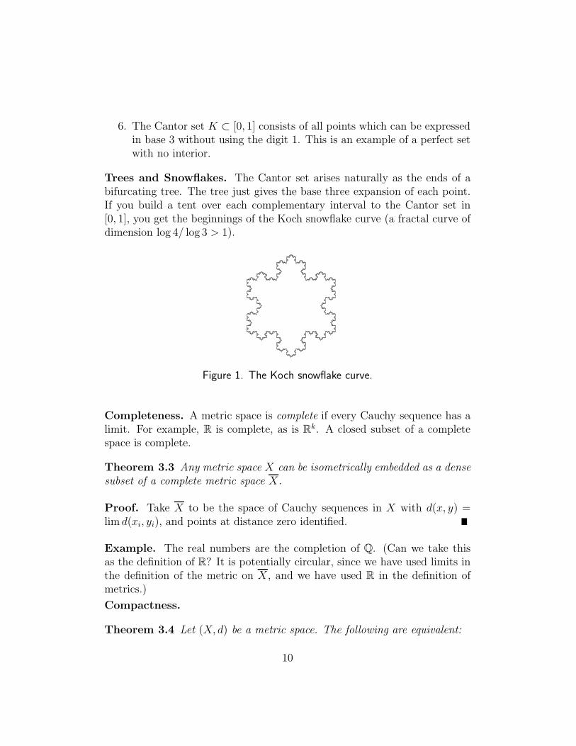
Trees and Snowflakes. The Cantor set arises naturally as the ends of abifurcating tree. The tree just gives the base three expansion of each point.If you build a tent over each complementary interval to the Cantor set in[0, 1], you get the beginnings of the Koch snowflake curve (a fractal curve ofdimension log 4/ log 3 > 1).
Figure 1. The Koch snowflake curve.
Completeness. A metric space is complete if every Cauchy sequence has alimit. For example, R is complete, as is Rk. A closed subset of a completespace is complete.
Theorem 3.3 Any metric space X can be isometrically embedded as a densesubset of a complete metric space X.
Proof. Take X to be the space of Cauchy sequences in X with d(x, y) =lim d(xi, yi), and points at distance zero identified.
Example. The real numbers are the completion of Q. (Can we take thisas the definition of R? It is potentially circular, since we have used limits inthe definition of the metric on X, and we have used R in the definition ofmetrics.)
Compactness.
Theorem 3.4 Let (X, d) be a metric space. The following are equivalent:
10
1. Every sequence in X has a convergent subsequence.
2. Every infinite subset of X has a limit point.
3. For every nested sequence of nonempty closed sets F1 ⊃ F2 ⊃ · · · inX,⋂Fi 6= ∅.
The proof is straightforward. When these conditions hold, we say X iscompact. More generally, a subset K ⊂ X is compact if these conditions holdfor the induced metric. Note that a compact subspace of X is automaticallyclosed.
Separability and open covers. A metric space is separable if it has acountable dense set. E.g. Rn is separable since Qn is dense.
Proposition 3.5 A compact metric space is separable.
Proof. Let En ⊂ X be a maximal collection of points separated by at least1/n. Then En has no limit point, so it must be finite; and
⋃En is dense.
Proposition 3.6 In a separable metric space, every open cover has a count-able subcover.
Proof. Suppose U covers X. Let (xi) be a countable dense set, and let Ui,n
be an element of U containing B(xi, 1/n) if such an element exists. The listof such Ui,n is countable, and for every x ∈ X there is a U ∈ U and i, n suchthat x ∈ B(xi, 1/n) ⊂ U ; thus
⋃Ui,n covers X.
Theorem 3.7 A metric space X is compact iff every open cover of X has afinite subcover.
Proof. Suppose X is compact, and let U be an open cover of X. By thepreceding results, we can assume U is a countable set U1, U2, . . .. ThenVi =
⋃i1 Uj is an increasing collection of open sets with
⋃Vi = X. Thus
Fi = X −Vi is a decreasing collection of closed sets with⋂Fi = ∅. It follows
that Fi = ∅ for some i, and hence⋃i
1 Uj = X.The converse is similar.
11
Non-example. The line R is not compact. Check that every property aboveis violated.
Theorem 3.8 Any interval I = [a, b] ⊂ R is compact.
Proof. Suppose E ⊂ I is an infinite set. Cut I into two equal subintervals.One of these, say I1, meets E in an infinite set. Repeating the process, weobtain a nested sequence I1 ⊃ I2 ⊃ I3 . . . such there is at least one pointxi ∈ E ∩ Ii. Since |Ii| = 2−i|I|, (xi) is a Cauchy sequence, and hence itconverges to a limit x ∈ I which is also a limit point of E.
Theorem 3.9 A subset E ⊂ Rn is compact iff it is closed and bounded.
Proof. A bounded set is contained in [a, b]n for some a, b and then the argu-ment above can be applied to each coordinate. Conversely, if E is unboundedthen a sequence xn ∈ E with |xn| → ∞ has no convergent subsequence.
Similar arguments show:
Theorem 3.10 A nonempty, compact, perfect metric space X is uncount-able. In fact, it contains a bijective copy of 2N, so |X| = |R|.
Remark: the continuum hypothesis. CH asserts that any uncoutnableset E ⊂ R satisfies |E| = |R|. Although this statement is undecidable, it canbe proved for many classes of sets. In particular, it holds if E is closed: inthis case either E is countable or it contains a closed, perfect set, and hence|E| = R. (To prove this statement, show the set of condensation pointsE ′ ⊂ E, i.e. points x such that |B(x, r) ∩ E is uncountable for all r > 0, isperfect.)
Theorem 3.11 If (X, d) is compact, then it is also complete.
Infinite cubes. Let X = [0, 1]N denote the infinite cube. Consider themetrics
d1(x, y) = sup |xi − ui| and d2(x, y) =∑
|xi − ui|/2i.
12
It is easy to see that X is complete in both metrics, and both spaces arebounded. However, (X, d2) is compact while (X, d1) is not! Note, for exam-ple, that the ‘basis points’ (en)i = δin satisfy d1(en, em) = 1 for all n < m,while d2(en, 0) = 2−n → 0.
A metric space (X, d) is totally bounded if for each r > 0 there is a finitecover of X by r-balls.
Theorem 3.12 A metric space is compact if and only if it is complete andtotally bounded.
In fact total boundedness allows one to extract a Cauchy sequence fromany infinite sequence, and then completeness insures it converges.
Connectedness. A metric space is disconnected if we can write X = U ⊔Vas the union of two disjoint, nonempty open sets. Otherwise it is connected.Note that U and V are also closed subsets of X.
Example. One can show that [0, 1] is connected, and hence any path con-nected space is connected. In particular, any convex subset of Rk is con-nected. There are sets which are connected but not path connected.
Morphisms. What should the morphisms be in the category of metricspaces? One choice would be isometries; these are like isomorphisms. Wecould also take sub-isometries, i.e. those satisfying
d(f(x), f(y)) ≤Md(x, y),
which can collapse large sets to points (i.e., have a nontrivial ‘kernel’); orLipschitz maps. But if we focus on convergent sequences are the fundamentalnotion in metric spaces, then the natural morphisms are continuous maps.
Continuity. A map f : X → Y between metric space is continuous if,whenever xn → x, we have f(xn) → f(x).
Theorem 3.13 A map f is continuous iff f−1(V ) is open for all open setsV ⊂ Y iff f−1(F ) is closed for all closed subsets F ⊂ Y .
Theorem 3.14 The continuous image of compact (or connected) set is com-pact (or connected).
The following result is one of the main reasons compactness is taught notjust to mathematicians but to economists, computer scientists and anyoneinterested in optimization.
13
Corollary 3.15 (Optima exist) A continuous function f : X → R on acompact space assumes its maximum and minima: there exist a, b ∈ X suchthat
f(a) ≤ f(x) ≤ f(b)
for all x ∈ X.In particular, f is bounded.
Corollary 3.16 (Intermediate values) If f : [a, b] → R is continuous,then f assumes all the values c ∈ [f(a), f(b)].
More generally, if f is a continuous function on a convex set X ⊂ Rk,then f(X) is an interval.
Homeomorphisms. In topology, the natural notion of isomorphism iscalled homeomorphism. A homeomorphism between two metric spaces Xand Y is a bijection f : X → Y such that both f and f−1 are continuous.That means X and Y are the same open sets.
Example: A square and a circle are homeomorphic; so are a coffee cup(with a handle) and a donut (or a compact disk). A torus is not homeomor-phic to a sphere (why not?!)
Theorem 3.17 If X is compact and f : X → Y is a bijection then f is ahomeomorphism.
Proof. If F ⊂ X is closed, then it is compact, so f(F ) is compact, andtherefore closed. This shows f−1 is continuous.
Exercise: give a proof that f−1 is continuous using sequences.
Nonexample. The map f : [0, 2π) → S1 ⊂ C given by f(x) = exp(ix) is abijection but not a homeomorphism.
Composition. It is immediate that continuous functions are closed undercomposition.
Theorem 3.18 The space C(X) of continuous function f : X → R formsan algebra, and f ∈ C(X) =⇒ 1/f ∈ C(X) whenever f has no zeros.
The main point one needs to use here is the important:
Lemma 3.19 If xn ∈ X is a convergent sequence or a Cauchy sequence,then xn is bounded.
14
Corollary 3.20 If an → a and bn → b in R, then anbn → ab.
Corollary 3.21 The polynomials R[x] are in C(R).
Question. Why is exp(x) continuous? A good approach is to show it is auniform limit of polynomials (see below). N.B. the function g : [0, 1] → R
given byg(x) = lim
n→∞xn
is also a limit of polynomials but not continuous!
Continuous functions on a compact set. We wish to give an interestingexample of a complete metric space besides a closed subset of Rk, and alsoshow the difference between completeness and compactness.
Let C[a, b] be the vector space of continuous functions f : [a, b] → R.Define a norm on this space by
‖f‖∞ = sup[a,b]
|f(x)|,
and a metric by
d(f, g) = ‖f − g‖∞ = sup |f(x) − g(x)|.This metric is finite because any continuous function on a compact space isbounded.
We will show:
Theorem 3.22 The metric space (C[a, b], d) is complete.
Bounded sets. First note that a closed ball in C[a, b] is not compact.For example, what should sin(nx) converge to? Or, note that we can findinfinitely many points in B(0, 1) with d(fi, fj) = 1, i 6= j.
Even worse, we can have fn ∈ C[a, b] such that fn(x) → g(x) for all x,but g is not continuous. Also, is it clear that d(f, g) is even finite?
The main point will be to use compactness of [a, b]. In fact the wholedevelopment works just as well for any compact metric space K. We defineC(K) just as before.
In particular, we can make the space of all bounded functions B(K) intoa metric space using the sup-norm as well, and we have C(K) ⊂ B(K).
Uniform convergence. We say a sequence of functions fn, g : X → R
converges uniformly if g−fn is bounded and ‖g−fn‖∞ → 0. If g (and hencefn) is bounded, this is the same as convergence in B(X).
15
Theorem 3.23 If fn : X → R is continuous for each n, and fn → g uni-formly, then g is continuous.
Proof. We illustrate the use of lim sup. Suppose xi → x in X. Then forany n, we have
|g(xi) − g(x)| ≤ |fn(xi) − fn(x)| + 2d(fn, g).
Letting i→ ∞, we have
lim sup |g(xi) − g(x)| ≤ 2d(fn, g).
Since n is arbitrary and d(fn, g) → 0, this shows g(xi) → g(x).
Corollary 3.24 If K is compact then C(K) is complete.
Proof. Let fi be a Cauchy sequence in C(K). Then fi(x) is a Cauchysequence in R for each x. Thus fi(x) → g(x) for each x. Moreover ‖g −fi‖∞ → 0 since d(fi, fj) → 0. Thus fi → g uniformly, and therefore g iscontinuous.
Note that compactness was used only to get distances finite. The sameargument shows that B(X) is complete for any metric space X, and C(X)∩B(X) is closed, hence also complete.
The quest for completeness: comparison with R. We obtained thecomplete space R by starting with Q and requiring that all reasonable limitsexist. We obtained C[0, 1] by a different process: we obtained completeness‘under limits’ by changing the definition of limit (from pointwise to uniformconvergence).
This begs the question: what happens if you take C[0, 1] and then passto the small set of functions which is closed under pointwise limits? Thisquestion has an interesting and complex answer, addressed in courses onmeasure theory: the result is the space of Borel measurable functions.
Monotone functions. One class of non-continuous functions that are veryuseful are the monotone functions f : R → R. These satisfy f(x) ≥ f(y)whenever x > y (if they are increasing) or whenever x < y (if they aredecreasing). If the strict inequality f(x) < f(y) holds, we say f is strictlymonotone.
16
Theorem 3.25 A map f : R → R is a homeomorphism iff it is strictlymonotone and continuous.
Theorem 3.26 A monotone function has at most a countable number ofdiscontinuities.
Note that limx→y− f(x) and limx→y+f(x) always exists.
Example; probability theory. Let qn be an enumeration of Q with n =1, 2, 3, . . . and let f(x) =
∑qn<x 1/2n. Then f is monotone increasing and its
points of discontinuity coincide with Q. Note that f increases from 0 to 1.Quite generally, if X is a random variable, then its distribution function
is defined by F (x) = P (X < x). In the example above we can take X = qnwith probability 1/2n. In fact, random variables correspond bijectively withmonotone functions that increase from 0 to 1, with a suitable convention ofright or left continuity.
The random variable X attached to f(x) above gives a random rationalnumber. This variable can be described as follows: flip a coin until it firstcomes up heads; if n flips are required, the value of X is qn.
4 Real sequences and series
The binomial theorem. The binomial theorem, which is easily proved byinduction, states that:
(1 + y)n = 1 + ny +
(n
2
)y2 + · · ·+ yn,
where(
ab
)= a!/(b!(a − b)!). The coefficients form Pascal’s triangle. We will
see that this algebra theorem can also be used to evaluate limits.
Some basic sequences. Perhaps the most basic fact about sequences isthat if |x| < 1 then xn → 0. But how would you prove this?
Here are more. Assume p > 0 and n→ ∞. Then:
1. np → ∞, i.e. 1/np → 0.
2. p1/n → 1.
3. n1/n → 1.
17
4. npxn → 0 if |x| < 1.
Note that the last includes the fact that xn → 0.These can be proved using L’Hopital’s rule, but more elementary proofs
are available. They are based on the fact that the binomial coefficient(
np
)
is a polynomial in n with coefficients that only depend on p. In particular,(np
)> Cnp > 0. One combines this with the binomial theorem itself to see
(1 + y)n ≥ Cpnpyp
for all n ≥ p and y > 0.For example, to prove an = n1/n − 1 → 0, we compute
n = (1 + an)n ≥ Cn2a2n
which shows an = O(1/√n). To prove npxn → 0, we may assume p is an
integer > 0; and we just have to show that if y > 0 then (1 + y)n > Cnp+1
for large n; this is true because
(1 + y)n >
(n
p+ 1
)yp+1 > Cnp+1
(where the constant depends on y).
Series. The notation∑an = S is just shorthand for bN =
∑N0 an → S.
The most important series in the world is the geometric series:
∞∑
0
xn =1
1 − x
for |x| < 1. This is proved by explicitly summing the first N terms by atelescoping trick, and using the fact that xN → 0. Equivalent, its evaluationis based on the factorization:
xn − 1 = (x− 1)(1 + x+ · · ·+ xn−1).
Note that for x = −1 this series seems to justify the statement that1 − 1 + 1 − 1 + 1 . . . = 1/2. Once we know that series behave well withrespect to integration, we can use this to justify e.g.
log(1 + x) =
∫ x
0
dt
1 + t= x− x2/x+ x3/3 − x4/4 + · · · ,
18
and hence 1 − 1/2 + 1/3 − 1/4 + · · · = log 2; and
tan−1(x) =
∫ x
0
dt
1 + t2= x− x3/3 + x5/5 − x7/7 + · · · ,
and hence π/4 = 1 − 1/3 + 1/5 − 1/7 + · · · .Acceleration. Often it is interesting just to find out if a series converges ornot. Here is a useful fact.
Theorem 4.1 Suppose a1 ≥ a2 ≥ a3 ≥ · · · ≥ 0. Then∑an converges if
and only if∑
2na2n converges.
Corollary 4.2 The series∑
1/np converges if and only if p > 1.
Note that if∑an converges then the tail tends to zero:
∑n≥N an → 0;
and an → 0. The harmonic series shows the latter condition is far from suffi-cient for convergence; while the former condition is equivalent to convergence,because it means the partial sums form a Cauchy sequence.
Sequences and series. Here is a nice example of an interplay betweensequences and series that is also mediated by the binomial theorem.
Theorem 4.3 (Defn. of e) We have lim(1 + 1/n)n =∑∞
0 1/n!.
Proof. First, note that∑
1/n! converges by comparison with say∑
1/2n.Now use the binomial theorem together with the fact that
1
k!≥(n
k
)(1
n
)k
=1
k!
k−1∏
0
(1 − j
n
)→ 1
k!
as n→ ∞ to conclude on the one hand that
(1 +
1
n
)n
=
n∑
0
(n
k
)(1
n
)k
≤n∑
0
1
k!,
and on the other hand that the reverse inequality holds because each indi-vidual term (for fixed k) converges to 1/k!.
19
Irrationality of e. It is well-known, and not too hard to prove, that eis transcendental. It is even easier to prove e is irrational: we have e =(Nq + ǫq)/q!, where 0 < ǫq < 1; while if e = p/q, then q!e − Nq = ǫq is aninteger.
Root and ratio test. The ratio test says that if lim sup |an+1/an| = r <1, then
∑an converges (absolutely). This proof is by comparison with a
geometric series C∑sn. with r < s < 1.
The root test gives the same conclusion, by the same comparison, iflim sup |an|1/n = r < 1. There are converse theorems if the limsup is a limitr > 1, but these are no more interesting than the fact that
∑an diverges if
|an| does not tend to zero (the nth term test).
Power series. The real virtue of the root test is the following.
Theorem 4.4 Given an ∈ C, let r = lim sup |an|1/n. Then∑anz
n con-verges uniformly on compact sets for all z ∈ C with |z| < 1/r.
For the proof just observe that∑fn converges uniformly if
∑ ‖fn‖∞ is finite.The conclusion is almost sharp: the series diverges if |z| > 1/r.
Example. The function exp(z) =∑zn/n! is well-defined for all z ∈ C,
because (ratio test) lim |z|/n→ 0 or because (root test) (n!)1/n ≥ (n/2)1/2 →∞.
Corollary 4.5 If f(x) =∑anx
n converges for |x| < R, then∫f and f ′(x)
are given in (−R,R) by∑anx
n+1/(n+ 1) and∑nanx
n−1.
Summation by parts. It is worth noting that differentiation and integra-tion have analogues for sequences. These can be based on the definition
∆an = an − an−1,
which satisfiesN∑
1
∆an = aN − a0
as well as the Leibniz rule
(∆ab)n = an∆bn + bn−1∆an.
20
Summing both sides we get the summation by parts formula:
N∑
1
an∆bn = aNbN − a0b0 −N∑
1
bn−1∆an.
(It is convenient to think of an, bn as being defined for all n, but for theequation above it is enough that they are defined for n ≥ 0; then ∆an and∆bn are defined for n ≥ 1.)
Example:
S =
N∑
1
n2 =
N∑
1
n2(∆n) = N3 −N∑
1
(n− 1)∆n2
= N3 −N∑
1
(n− 1)(2n− 1) = N3 − 2S +N∑
1
(3n− 1)
= N3 − 2S + 3N(N + 1)/2 −N,
which gives
S =N(2N2 + 3N + 1)
6·
5 Differentiation in one variable
Differentiation. Let f : [a, b] → R. We say f is differentiable at x if
limy→x
f(y) − f(x)
y − x=: f ′(x)
exists (note that if x = a or b, the limit is one-sided); equivalently, if
f(y) = f(x) + f ′(x)(y − x) + o(y − x).
If f ′(x) exists for all x ∈ [a, b], we say f is differentiable .
Calculating derivatives. The usual procedures of calculus (for computingderivatives of sums, products, quotients and compositions) are readily verifiedfor differentiable functions. (Less is needed, e.g. all but the chain rule workfor functions just differentiable at x.) In particular we will later use:
Theorem 5.1 The derivative of a polynomial∑anx
n is given by∑nanx
n−1.
21
Continuity. If f is differentiable then it is also continuous. However thereexist functions which are continuous but nowhere differentiable. An exampleis f(x) =
∑∞1 sin(n!x)/n2; the plausibility is seen by differentiating term by
term.
Properties of differentiable functions.
Theorem 5.2 Let f : [a, b] → R be differentiable. Then:
1. If f(a) = f(b) then f ′(c) = 0 for some c ∈ (a, b).
2. There is a c ∈ (a, b) such that
f(b) − f(a) = f ′(c)(b− a).
3. If f ′(a) < y < f ′(b), then f ′(c) = y for some c ∈ (a, b).
Proof. (1) Consider a point c where f achieves it maximum or minimum.(2) Apply (1) to g(x) = f(x) −Mx, where M = (f(b) − f(a))/(b − a). (3)Reduce to the case y = 0 and again consider an interior max or min of f .
Jumps. To see (3) is interesting, it is important to know that there existexamples where f ′(x) is not continuous! By (3), if f ′(x) exists everywhere,it cannot have a jump discontinuity.
Corollary 5.3 If f is differentiable and f ′ is monotone, then f ′ is continu-ous.
Taylor’s theorem. This is a generalization of the mean-valued theorem.
Theorem 5.4 If f : [a, b] → R is k-times differentiable, then there exists anx ∈ [a, b] such that
f(b) =
(k−1∑
0
f (j)(a)
j!(b− a)j
)
+f (k)(x)
k!(b− a)k.
Proof. Subtracting the Taylor polynomial from both sides, we can alsoassume that f and its first k − 1 derivatives vanish at 0. Suppose we alsoknew f(b) = f(a). Then there would be an x1 ∈ [a, b] such that f ′(x1) = 0,
22
and then (by induction) an xi ∈ [a, xi−1] such that f (i)(xi) = 0; and we couldtake x = xk.
To reduce to this case, we consider instead the function g(x) = f(x) −M(x−a)k, where M = (f(b)− f(a))/(b−a)k is chosen so g(b) = g(a). Thenwe find an x such that g(k)(x) = 0. But this means f (k)(x) = k!M , whichgives what we want.
Remark. There exist nontrivial functions whose Taylor polynomials aretrivial, e.g. f(x) = exp(−1/x2) at x = 0.
Spaces of differentiable functions. We let Ck[a, b] denote the space ofk-times differentiable functions with the norm
‖f‖Ck =k∑
0
‖f (j)‖∞.
Theorem 5.5 If fn ∈ C1[a, b], fn → f uniformly and f ′n → g uniformly,
then f ′ = g.
Proof. We first remark that if fn → f uniformly and xn → x, then fn(xn) →f(x).
Now for x, y ∈ [a, b], we have by the mean value theorem
f(y) − f(x)
y − x= lim
n
fn(y) − fn(x)
y − x= lim f ′
n(cn) = g(c)
for some cn and c in [x, y]. (Here c is any limit point of cn). Taking the limitas y → x gives f ′(x) on the left and g(x) on the right.
Corollary 5.6 The space Ck[a, b] is complete.
Corollary 5.7 Any power series f(x) =∑anx
n defines a C∞ function onits region of convegence.
Proof. Note that∑anx
n and∑nanx
n−1 have the same radius of con-vergence, and both converge uniformly; the term-by-term differentiation isjustified by the results above.
We now have rigorously proved, for example, that y = ex and y = sin(x)solve the differential equations y′ = y and y′′ + y = 0 respectively.
23
6 Integration in one variable
Integration of continuous functions. One of the most fundamental op-erators on C[a, b] is the operator of integration, Ib
a : C[a, b] → R. It can bedescribed axiomatically as follows.
Theorem 6.1 There is a unique linear map Iba : C[a, b] → R, defined for
every interval [a, b], such that:
1. If f ≥ 0 then Iba(f) ≥ 0;
2. If a < c < b then Iba(f) = Ic
a(f) + Ibc (f); and
3. I(1) = b− a.
Lebesgue number. For the proof, we begin with the following remark. Let⋃Ui be an open covering of a compact set K. Then f(x) = supi d(x,X−Ui)
is a positive continuous function, which is therefore bounded below. Thusthere is a number r such that for every x ∈ K, we have B(x, r) ⊂ Ui forsome i. This radius r is called the Lebesgue number of the covering.
Uniform continuity. A function on a metric space, f : X → R, is said tobe uniformly continuous if there is a positive function h(r) → 0 as r → 0such that
d(x, y) < r =⇒ |f(x) − f(y)| < h(r).
The function h(r) is called the modulus of continuity of f . (It is not unique,just an upper bound.)
For example, if f : [a, b] → R has |f ′(x)| ≤ M , then we may take h(r) =Mr. Such functions are said to be Lipschitz continuous; they can increasesdistances by only a bounded amount. The function f(x) =
√x on [0, 1] is
not Lipschitz, but it is Holder continuous: it satisfies
|f(x) − f(y)| ≤ M |x− y|α
for some M,α > 0. In fact we can take α = 1/2, because
|√x−√y| · |√x+
√y| ≤ |x−y| ≤ |x−y|1/2|x−y|1/2 ≤ |x−y|1/2 · |√x+
√y|.
Theorem 6.2 Any continuous function f on a compact spaceK is uniformlycontinuous.
24
Proof. We must show for each h > 0 there is an r > 0 such that d(x, y) <r =⇒ |f(x) − f(y)| < h. Cover R by open intervals (Ii) of length h.Then their preimages Ui give an open cover of K (which can be reduced toa finite subcovering). Let r > 0 be the Lebesgue number of this covering. If|x− y| < r then x, y ∈ Ui for some i, and hence f(x), f(y) ∈ Ii which implies|f(x) − f(y)| ≤ h.
Sketch of the proof of Theorem 6.1. Although we are interested in con-tinuous functions, it is useful to first define the integral I(s) of step functionss(x). Then we check that I(s) satisfies the axioms above, with continuousfunctions replaced by step functions. Especially, I(s) is linear. Then weobserve that any function Ib
a(f) satisfying the axioms above also satisfiesI(s) ≤ Ib
a(f) ≤ I(S) whenever s < f < S. Therefore we define
I−(f) = sups<f
I(s), I+(f) = inff<S
I(S).
By uniform continuity we find s, S with s < f < S and |S − s| < ǫ, whichshows I−(f) = I+(f) and shows the existence of such the linear map Ib
a oncontinuous functions. A similar argument proves uniqueness.
Corollary 6.3 The map I : C[a, b] → R is continuous; in fact, |I(f)| ≤|a− b|‖f‖∞.
Corollary 6.4 If fn is a sequence of continuous functions and fn → g uni-formly, then
∫ b
afn →
∫ b
ag.
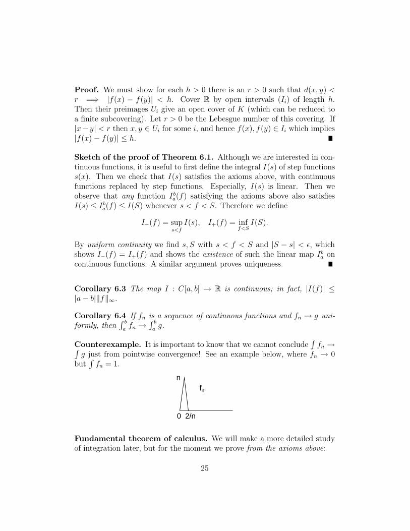
Counterexample. It is important to know that we cannot conclude∫fn →∫
g just from pointwise convergence! See an example below, where fn → 0but
∫fn = 1.
2/n
n
nf
0
Fundamental theorem of calculus. We will make a more detailed studyof integration later, but for the moment we prove from the axioms above:
25
Theorem 6.5 If f : [a, b] is continuous and F (x) =∫ x
af(t) dt, then F ′(x) =
f(x).
Proof. We have (1/t)(F (x+ t) − F (x)) = (1/t)∫ x+t
xf(t) dt→ f(x).
Corollary 6.6 If f ′(x) is continuous, then∫ x
af ′(t) dt = f(x) + C.
Note: if we just assume f(x) is differentiable, then f ′(x) might not evenhave an integral.
Limits of differentiable functions, reprise. Integration gives an alter-nate proof of Theorem 5.5 above, which asserts if fn ∈ C1[a, b], fn → funiformly and f ′
n → g uniformly, then f ′ = g.
Proof. We have
fn(x) − fn(a) =
∫ x
a
f ′n;
taking limits on both sides gives
f(x) − f(a) =
∫ x
a
g
and hence f ′(x) = g(x).
Riemann integrability. Let f : [a, b] → R be an arbitrary function. Wesay f is Riemann integrable if
sup
∫g : g ∈ C[a, b], g ≤ f
= inf
∫h : h ∈ C[a, b], h ≥ f
,
and denote the common value of these quantities by∫ b
af(x) dx.
Theorem 6.7 Any piecewise continuous function is in R. If f ∈ R then fis bounded.
Theorem 6.8 A bounded function f : [a, b] → R is Riemann integrable iffits points of discontinuity form a set of measure zero.
26
Here the measure of a set E is the infimum of∑ |Ii| over all countable
collections of open intervals such that E ⊂ ⋃ Ii.
Examples. The indicator function of Q gives an example of a function thatis not Riemann integrable. On the other hand, the function f(x) = 1/q ifx = p/q and f(x) = 0 otherwise, is discontinuous just on the rationals, so itis integrable.
Holder’s inequality. It is useful to define for p ≥ 1 the norms
‖f‖p =
(∫|f |p)1/p
.
These satisfy the triangle inequality (exercise) and we have the important:
Theorem 6.9 (Holder’s inequality) If f, g ∈ C[a, b] then
∣∣∣∣∫ b
a
fg
∣∣∣∣ ≤ ‖f‖p ‖g‖q.
whenever 1/p+ 1/q = 1.
The case p = q = 2 gives Cauchy-Schwarz.
Proof. First check Young’s inequality xy ≤ xp/p + yq/q. Then by homo-geneity we can assume ‖f‖p = ‖g‖q = 1, and deduce
∫|fg| ≤
∫|f |p/p+
∫|g|q/q = 1.
(Proof of Young’s inequality. Draw the curve yq = xp, which is the sameas the curve y = xp−1 or x = yq−1 (since pq = p+q). Then the area inside therectangle [0, a]× [0, b] is bounded above by the sum of ap/p, the area betweenthe graph and [0, a], and bq/q, the area between the graph and [0, b].)
(Brute force proof: minimize f(x, y) = xp/p + yq/q subject to g(x, y) =xy = a. Then by the method of Lagrange multipliers, we have (y, x) =λ(xp−1, yq−1). This gives xy = λxp = λyq and hence xp/p+yq/q = λxy. Andit also implies x = λ2(xp−1)q−1 = λ2x, so λ = 1.)
Lebesgue theory. The completions of the space C[a, b] with respect tothe norms above are the Lebesgue spaces Lp[a, b]. Their elements consist ofmeasurable functions, to be discussed in Math 114.
27
Clearly |I(f)| ≤ ‖f‖1. So if fn ∈ C[a, b] are a Cauchy sequence in L1,one should expect I(lim fn) = lim I(fn). This gives the ‘right guess’ e.g. forthe indicator function of the rational numbers.
The little ℓp spaces are defined using sequences instead of functions, andsetting
‖a‖p =(∑
|an|p)1/p
.
Holder’s inequality holds here as well, and these spaces are complete. In factℓp is the dual of ℓq if p > 1; and ℓ1 is the dual of the space c0 of sequenceswhich converge to zero.
The ℓp norms on Rn also make sense and their unit balls are easily visu-alized for n = 2, 3.
The integral test. We recall there is a close relationship with series anintegrals: if f(x) ≥ 0 is decreasing, then
∑∞1 f(n) and
∫∞1f(x) dx either
both converge or both diverge.
Riemann-Stieltjes integration. Let α : [a, b] → R be any monotoneincreasing function. Then for any f ∈ C[a, b] we can define
∫ b
a
fdα
by the same axioms as before, but requiring that∫ d
c
dα = α(d) − α(c) = ∆α.
Unwinding the definition, we find that∫fdα ≈
∑f(xi)∆αi
for any fine enough division of [a, b] such that f has small variation over each
piece. In particular, there is again a unique such integral∫ b
afdα defined for
all f ∈ C[a, b], and it can be extend to a larger class of functions R(α) withmild discontinuities.
Probability and δ functions. If α is the distribution function of a randomvariable X, then
∫fdα = E(f(X)). For example, if H(x) = 1 for x > 0 and
0 otherwise, then∫f dH = f(0). More generally, if
∑ai <∞ then
∫f d(∑
aiH(x− bi))
=∑
aif(bi).
28
Note that H is not in R(H) on [−1, 1]!
Theorem 6.10 Any continuous function is in R(α), and if α is continuous,then any piecewise continuous function is in R(α).
The differentiable case. If α ∈ C1[a, b], we have ∆αi = α′(ci)∆xi, bythe intermediatve value theorem, where ci is very close to xi. Using uniformcontinuity of α′(x), we find:
∫f(x) dα(x) =
∫f(x)α′(x) dx.
The pullback formula. Suppose α : [a, b] → [c, d] is an orientation-preserving homeomorphism. Then the integral of dα over any subintervalJ is just the length of α(J). From this we see that:
∫ d
c
f(u) du =
∫ b
a
f(α(x))dα(x).
The second interval is obtained by just formally substituting u = α(x) in thefirst.
Example. The combination of the two formulas above justifies the usualchange of variables formula, e.g. since sin : [0, π/2] → [0, 1] is a homeomor-phism, we can set y = sin(t) and compute
∫ 1
0
√1 − y2 dy =
∫ π/2
0
√1 − sin2(t) d sin(t) =
∫ π/2
0
cos2(t) dt = π/4
(since∫
cos2 + sin2 =∫
1). Of course this gives 1/4 the area of a unit circle.
Counting example. Let 0 < x1 < x2 < x3 . . . xn be a finite set of realnumbers, and let N(x) be the number of i such that xi > x. Suppose f(x)is smooth for x ≥ 0 and f(0) = 0. Then integration by parts shows:
∑f(xi) = −
∫f(x)dN(x) =
∫ ∞
0
f ′(x)N(x) dx.
For example,∑xi =
∫N(x) dx.
29
7 Algebras of continuous functions
In this section we prove some deeper properties of the space C(X).
Compactness: Arzela–Ascoli. LetK be a compact metric space as above.A family of functions F ⊂ C(K) is equicontinuous if they all have the samemodulus of continuity h(r).
Theorem 7.1 The closure of F is compact in C(K) iff F is bounded andequicontinuous.
Proof. The condition that F is totally bounded in the metric space C(K)translates into equicontinuity.
Example. The functions fn(x) = sin(nx) are not equicontinuous on C[0, 1],but the functions with |f ′
n(x)| ≤ 1 are. Thus any sequence of boundedfunctions with bounded derivatives has a uniformly convergent subsequence.
Approximation: Stone–Weierstrass.
Theorem 7.2 (Weierstrass) The polynomials R[x] are dense in C[a, b].
This result gives a nice occasion to introduce convolution and approxi-mations to the δ-function. First, the convolution is defined by
(f ∗ g)(x) =
∫
s+t=x
f(s)g(t) dt =
∫f(x− t)g(t) dt =
∫g(x− t)f(t) dt.
To make sure it is well-defined, it is enough to require e.g. that both functionsare continuous and one has compact support. Note that:
‖f ∗ g‖∞ ≤ ‖f‖infty‖g‖1.
From this one can readily verify that f ∗ g(x) is continuous. (Note: use thefact that if g has compact support, and gt(x) = g(x+ t), then ‖gt − g‖ → 0as t→ 0; this is a restatement of uniform continuity.)
The convolution inherits the best properties of both functions; e.g. if fhas a continuous derivative, then so does f ∗ g, and we have (f ∗ g)′(x) =(f ′ ∗ g), as can easily be seen from the formula above. Thus shows:
If f is a polynomial of degree d, then so is f ∗ g(x).
30
This can also be seen directly, using the fact that:
∫(t− x)ng(t) dt =
∑(n
k
)(−x)k
∫tkg(t) dt;
or conceptually, by noting that the polynomials of degree d form a closed,translation invariant subspace of C(R).
Approximate identities. We say a sequence of functions Kn(x) ≥ 0 is anapproximate identity if
∫Kn = 1 for all n and
∫|x|>ǫ
Kn → 0 for all ǫ > 0.
Theorem 7.3 If f is a compactly supported continuous function, then f ∗Kn → f uniformly.
Proof. We have |f | ≤ M for some M , and f is uniformly continuous, saywith modulus of continuity h(r). Suppose for example we wish to comparef(0) and (Kn ∗ f)(0). Since Kn ∗ 1 = 1, we may assume f(0) = 0. Choose rsuch that h(r) < ǫ and N such that
∫|x|>r
Kn < ǫ. Then splitting the integral
into two pairs at |x| = r, we find
|(Kn ∗ f)(0)| =
∣∣∣∣∫Kn(x)f(−x) dx
∣∣∣∣ ≤ h(r) +Mǫ ≤ (1 + ǫ)M.
Example. Let Kn(x) = an(1 − x2)n for |x| ≤ 1, and 0 elsewhere, where an
is chosen so∫Kn = 1. Then Kn(x) is an approximate identity.
To see this, we first note that (1−x2)n ≥ 1/2 if 1−x2 > (1/2)1/n ≈ 1−Cn,i.e. if |x| < C/
√n; this shows
∫(1 − x2)n ≥ C/
√n and hence an = O(
√n).
Now suppose |x| > r. Then Kn(x) = O(√n(1 − r2)n) → 0, i.e. Kn → 0
uniformly on |x| > r. It follows that∫|x|<r
Kn → 1.
Proof of Weierstrass’s theorem. We may suppose [a, b] = [0, 1], andadjusting by a linear function, we can assume f(0) = f(1) = 0. Extend fto the rest of R by zero. As above, choose Kn(x) = an(1 − x2)n for |x| ≤ 1,and 0 elsewhere, where an is chosen so
∫Kn = 1. Then pn = Kn ∗ f → f
uniformly on R. By differentiating, one can see that pn|[0, 1] (like Kn|[−1, 1])is a polynomial of degree 2n or less, because Kn ∗ f |[0, 1] is independent ofwhether we cut off the polynomial Kn or not.
31
Theorem 7.4 (Stone) Let A ⊂ C(X) be an algebra of real-valued functionsthat separates points. Then A is dense.
Sketch of the proof. Replace A by its closure; then we must show A =C(X). Since A is an algebra, f ∈ A =⇒ P (f) ∈ A for any polynomialP (x). Since |x| is a limit of polynomials (by Weierstrass’s theorem), we find|f | is in A. This can used to show that f, g ∈ A =⇒ f ∧ g, f ∨ g are both inA. The proof is completed using separation of points and compactness.
Complex algebras. This theorem does not hold as stated for complex-valued functions. A good example is the algebra A of polynomials in z inC(S1). These all satisfy
∫zf |dz| = 0 and this property is closed under
uniform limits, so g(z) = z is not in the closure. If, however we require thatA is a ∗-algebra (it is closed under complex conjugation), then the Stone-Weierstrass theorem holds as stated for complex functions as well.
Fourier series. Let S1 = R/2πZ. We make the space of continuous complexfunctions C(S1) into an inner product space by defining:
〈f, g〉 =1
2π
∫ 2π
0
f(x)g(x) dx.
In particular,
‖f‖22 = 〈f, f〉 =
1
2π
∫|f |2.
This inner product is chosen so that en = exp(inx) satisfies 〈ei, ej〉 = δij.The Fourier coefficients of f ∈ C(S1) are given by
an = 〈f, en〉.
If f =∑N
−N bnen, then an = bn.
Convergence of Fourier series: Fejer and Dirichlet. One of the mainconcerns of analysts for 150 years has been the following problem: givena function f(x) on S1, in what sense is f represented by its Fourier series∑an exp(inx)?
Trig polynomials. Let An ⊂ C(S1) denote the finite-dimensional subspacespanned by (e−n, . . . , en) and let A =
⋃An be the space of trigonometric
polynomials. Clearly A is an algebra, closed under complex conjugation.Thus the Stone-Weierstrass theorem shows:
32

Theorem 7.5 The algebra A is dense in C(S1) in the uniform norm, andhence also in the L2 norm.
Here we have used the fact that ‖f‖22 ≤ ‖f‖∞.
Theorem 7.6 If f ∈ C(S1), then f is determined by its Fourier series.
In other words, two f with the same Fourier series are equal.More precisely, we have:
Theorem 7.7 For any f ∈ C(S1) we have (1/2π)∫|f |2 =
∑ |ai|2.
Proof. Let fn =∑a
−n aiei. This is just the projection of f to An (say inthe span of An and f). Thus the usual finite-dimensional results on Hilbertspace imply that
n∑
−n
|ai|2 = ‖fn‖2 ≤ ‖f‖2,
and so the infinite sum∑ |ai|2 is also bounded by ‖f‖2.
For the reverse direction, observe that by density of A, for every ǫ > 0there exists an n and a g ∈ An such that ‖f−g‖2 ≤ ǫ. But fn is closest pointin An to f , and thus fn → f in the L2 norm. In particular, ‖f‖2 =
∑ |ai|2.
So if continuous functions f and g have the same Fourier series, then∫|f − g|2 = 0 so f = g.
Classical questions. Now how can one recover f from an?It is traditional to write SN(f) =
∑N−N an(f) exp(inx). The simplest
answer to the question is not too hard to establish: so long as f ∈ L2(S1),we have ∫
|f − SN(f)|2 → 0
as N → ∞.The question of pointwise convergence is equally natural: how can we
extract the value f(x) from the numbers an? Of course, if f is discontinuousthis might not make sense, but we might at least hope that when f(x) iscontinuous we have SN(f) → f pointwise, or maybe even uniformly. In thisdirection we have:
33
Theorem 7.8 If f(x) is C2, then an = O(1/n2) and thus SN(f) convergesto f uniformly.
In fact we have:
Theorem 7.9 (Dirichlet) If f(x) is C1, then SN(f) converges uniformlyto f .
The proof is based on an analysis of the Dirichlet kernel
DN =
N∑
−N
exp(inx) =sin((N + 1/2)x)
sin(x/2)·
Convolution. In this setting it is useful to define convolution with a factorof 2π, i.e.
(f ∗ g)(x) =1
2π
∫f(y)g(x− y) dy.
Note that if an = 〈f, en〉 then
anen(x) =1
2π
∫f(y)en(y)en(x) dy =
1
2π
∫f(y)en(x− y) dy = (f ∗ en)(x),
(in particular, ei ∗ ej = δijei), and thus SN(f) = f ∗DN . Dirichlet’s proof isbased on an analysis of this convolution. Note also that if f =
∑aiei and
g =∑biei then (f ∗ g) =
∑aibiei.
Dirichlet’s proof . . . left open the question as to whether the Fourierseries of every Riemann integrable, or at least every continuous,function converged. At the end of his paper Dirichlet made itclear he thought that the answer was yes (and that he would soonbe able to prove it). During the next 40 years Riemann, Weier-strass and Dedekind all expressed their belief that the answer waspositive. —Korner, Fourier Analysis, §18.
In fact this is false!
Theorem 7.10 (DuBois-Reymond) There exists an f ∈ C(S1) such thatsupN |SN(f)(0)| = ∞.
34
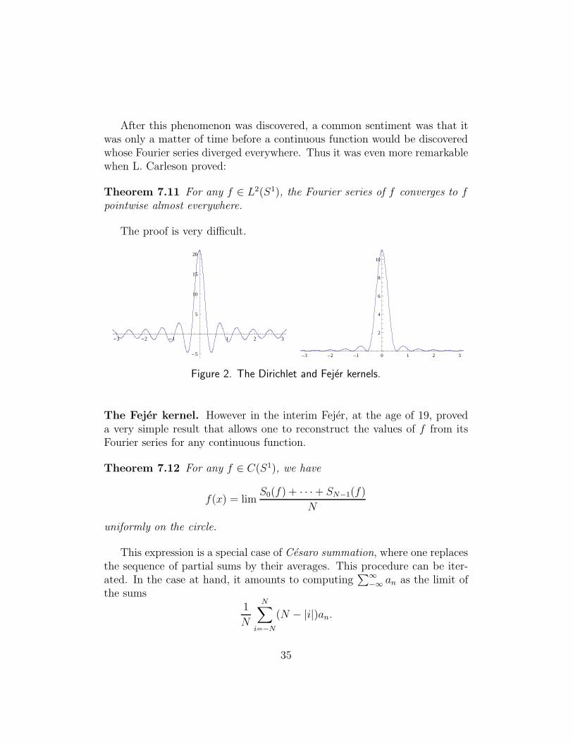
After this phenomenon was discovered, a common sentiment was that itwas only a matter of time before a continuous function would be discoveredwhose Fourier series diverged everywhere. Thus it was even more remarkablewhen L. Carleson proved:
Theorem 7.11 For any f ∈ L2(S1), the Fourier series of f converges to fpointwise almost everywhere.
The proof is very difficult.
-3 -2 -1 1 2 3
-5
5
10
15
20
-3 -2 -1 0 1 2 3
2
4
6
8
10
Figure 2. The Dirichlet and Fejer kernels.
The Fejer kernel. However in the interim Fejer, at the age of 19, proveda very simple result that allows one to reconstruct the values of f from itsFourier series for any continuous function.
Theorem 7.12 For any f ∈ C(S1), we have
f(x) = limS0(f) + · · · + SN−1(f)
N
uniformly on the circle.
This expression is a special case of Cesaro summation, where one replacesthe sequence of partial sums by their averages. This procedure can be iter-ated. In the case at hand, it amounts to computing
∑∞−∞ an as the limit of
the sums1
N
N∑
i=−N
(N − |i|)an.
35
Approximate identities. The proof of Fejer’s result again uses approxi-mate identities.
If we let
TN(f) =S0(f) + · · · + SN−1(f)
N,
then TN(f) = f ∗ FN where the Fejer kernel is given by
FN = (D0 + · · ·DN−1)/N.
Of course∫FN = 1 since
∫Dn = 1. But in addition, FN is positive and
concentrated near 0, i.e. it is an approximation to the identity. Indeed, wehave:
FN(x) =sin2(Nx/2)
N sin2(x/2)·
To see the positivity more directly, note for example that
(2N + 1)F2N+1 = z−2N + 2z−2N+1 + · · ·+ (2N + 1) + · · · 2z2N−1 + z2N
= (z−N + · · · zN )2 = D2N ,
where z = exp(ix). For the concentration near zero, observe that if |x| >1/(ǫ
√N), then |FN(x)| ≥ ǫ or so.
Modern questions. Perhaps a better question is: given any (an) ∈ ℓ2, isthere some function on S1 such an as its Fourier coefficients?
The answer again leads into the Lebesgue theory. If we let L2(S1) de-note the metric completion of C(S1) in the L2 norm, it is then clear thanℓ2 ∼= L2(S1); so the only issue is, how to interpret elements of this metriccompletion as functions?
Why sin(x) and cos(x)? Why, among all the functions in C(S1), are wefocusing on en(x) = cos(x) + i sin(x)? The reason ultimately has to do withrepresentation theory of the group G = S1 on C(S1). The spaces Vn = Cen
are invariant under the action of G by (gf)(x) = f(g−1x), and they are theonly such. So the decomposition of a function into its Fourier components isan attempt to make precise the statement
C(S1) = ⊕Vn,
in other words an attempt to decompose C(S1) into an infinite sum of itsirreducible subspaces for the action of G.
36
8 Differentiation in several variables
We now turn to the calculus of functions on domains in Rn, and more generalto the theory of smooth maps from Rn to Rm.
Differentiation. Let U ⊂ Rn be open. We say f : U → Rm is differentiableat x ∈ U if there is a linear map L : Rn → Rm such that
f(x+ t) = f(x) + L(t) + o(|t|).
(This means |f(x+ t) − f(x) − L(t)|/|t| → 0 as t→ 0.) Note that t ∈ Rn isa tangent vector in the domain of f , and that L(t) ∈ Rm is a tangent vectorin the range.
In this can we write f ′(x) = Df(x) = L ∈ Hom(Rn,Rm). Note that thespace Hom(A,B) of maps between normed vector spaces inherits a naturalnorm, given by
‖T‖ = supv 6=0
|Tv|/|v|.
(Use compactness of the unit ball to see this is finite.)We say f ∈ C1(U) if it is differentiable at every point, and the map
Df : U → Hom(Rn,Rm) is continuous.In terms of the standard basis, Df is just the matrix (Df)ij = dfi/dxj.
Theorem 8.1 If f is differentiable at x then so is each coordinate function,and Df = (dfi/dxj).
In other words,
∆f ≈∑
j
(dfi/dxj)∆xj .
From the definitions we easily get:
Theorem 8.2 (Chain Rule) If g is differentiable at x and f is differen-tiable at g(x), then
D(f g)(x) = (Dg(x)) Df(g(x)).
Theorem 8.3 We have f ∈ C1(U,Rn) iff dfi/dxj exists and is continuousfor all i, j.
37
One direction is easy: if f ∈ C1, then dfi/dxj is continuous. But theconverse is subtle! The existence of dfi/dxj for all i, j need not imply that fis continuous!
Example: Let f(x, y) = x cos2(θ) on R2, with f(0) = 0, where (x, y) =(r cos θ, r sin θ). Then df/dx = 1 and df/dy = 0 at (x, y) = (0, 0), and bothderivatives exist at every other point as well. But f(t, t) = t/2, which is notwell-approximated by Df(0, 0)(t, t) = t.
Proof of Theorem 8.3. We can reduce to the case where f = f(x1, . . . , xn).Let fj = df/dxj. Let t = (t1, . . . , tn) ∈ Rn be small. By the mean-valuedtheorem, we have
f(x+ t) = f(x) + (f1(x1)t1, . . . , f(xn)tn)
with xi in the cube of size |t| around x. Then since each fi is continuous, wehave fi(xi) = fi(x) + o(1). Thus
f(x+ t) = f(x) +∑
fi(x)ti + o(|t|)
which means f is differentiable.
Mean-value type results. There is no strict analogue of the mean-valuetheory, since e.g. f(t) = (sin(t), cos(t)) satisfies f(0) = f(2π) but nowheredoes f ′(t) = 0. However we do have:
Theorem 8.4 If f : [a, b] → Rm is differentiable, then
|f(a) − f(b)| ≤ |b− a| sup |f ′(t)|.
Proof. Let v be a unit vector in the direction f(b) − f(a), and let g(t) =〈f(x) − f(a), v〉. Then g(a) = 0 and |g′(t)| ≤ |f ′(t)| (by Cauchy-Schwarz),and hence |g(b)| = |f(a) − f(b)| satisfies the stated bound.
The same bound applies if f : U → Rm is a map in several variables, ifwe replace |f ′(t)| by ‖Df(t)‖.Curves, functions and maps. There are really 3 different flavors of mapsto be studied. The first are curves f : R → Rn. These have a rather simple,one-variable-like theory, since Df = (f ′
1, . . . , f′n) : R → Rn is a map of the
same type.
38
The second are functions f : Rn → R. These have a richer theory,since e.g. f−1(0) can be a rather complicated, singular object. Also, thehigher derivatives of order k have nk indices. The functions will also giverise to the exterior algebra generated by the forms df , which will be crucialin integration.
The final and most general case are maps f : Rn → Rm. Here the mainresults say the local behavior of f near p is sometimes controlled by Df(p).E.g. if Df is injective, then f is locally injective.
Curves of pursuit. Let f : R → Rn be a smooth path. Then the derivativesf ′ and f ′′ are of the same form. If |f ′(x)| = 1 we say the path is paramterizedby arclength. In this case, f ′′(t) is the curvature vector and f ′′′(t) is thetorsion. At f(t), the path is well-approximated by a circle of radius r =1/|f ′′(t)| whose center is in the direction f ′′(t).
Puzzle: 4 beetles start at the vertices of a unit square and each moves atunit speed towards the next. What happens?
Answer: they remain on the vertices of a square of side 1 − t until thecollide at time one. This is because the distance from one beetle to the nextdecreases at unit speed.
Followup 1: how many degrees does a beetle rotate before it collides withrest?
Answer: By the same reasoning, the distance from the origin at time t isjust d(t) = (1 − t)/
√2. If the initial position is P (0) ∈ R2, then the angle
between P (t) and P ′(t) is constant. Thus dθ/dt = C/d(t) for some constantC. Since 1/d(t) blows up like 1/(1 − t), the total angle (winding number) isinfinite.
Followup 2: what is the curve traced out by P , exactly? Its characteristicproperty is that the angle between P (t) and P ′(t) is constant. Let us param-eterize the curve by its angle, i.e. write it in polar coordinates as r = f(θ).Then the quantity r′/r control the angle between the curve and its radius.So r′ = ar for some a, and hence r = exp(aθ).
Alternatively, the curve is swept out by s 7→ λs in C, for some complexnumber λ. (Actually we need to know log λ). Note that if f(s) = exp(Ls),then f ′(0) = L. So the beetle curve for the square is traced out by s 7→exp(s(1 + i)). Equivalently, we want r′ = r, which gives r = exp(θ). (Thenreiθ = eθeiθ = e(1+i)θ.)
Note that these curves are invariant under multiplication by λ; they are‘self-similar’.
39
Followup 3: What happens if you have N beetles on a unit circle, equallyspaced? You get a logarithmic spiral with a different, smaller angle, namely(2π/N).
Followup 4:What if you have N beetles on an ellipse? Explain the relationto curvature.
Differential equations. We remark that the solution of a linear differentialequation of order n in one variable, with given initial conditions, e.g.
f (n)(t) =
n−1∑
0
aif(i)(t),
can be reduced to the solution of a particular equation of the form
F ′(t) = AF (t)
where F : R → Rn, and F (0) is specified. Indeed, we just set
F (t) = (Fi(t)) = (f(t), f ′(t), . . . , f (n−1)(t)),
and let A be the companion matrix of the associated polynomial. (Putdifferently, F ′ = (F2, F3, . . . ,
∑aiFi+1).)
Theorem 8.5 The equation F ′(t) = AF (t) has a unique solution for a giveninitial value F (0).
Proof. Existence follows using the exponential: set F (t) = exp(tA)F (0).For uniqueness, suppose we have two solutions; then their difference satisfies|F ′(t)| ≤ C|F (t)| and F (0) = 0. But then (log |F |)′ ≤ C and hence |F (t)| ≤exp(Ct)|F (0)| = 0.
Factorization and diagonalization. If A = diag(λi) is diagonal, thesolution is very simple — since eA = diag(eλi). Of course this need not be
the case — if A = ( 0 1−1 0 ) then etA =
(cos(t) sin(t)− sin(t) cos(t)
).
As usual, this linear algebra is simpler of the complex numbers. In par-ticular, if P (f) = (
∑anD
n)(f) factors as∏
(D− λi), where D = d/dt, thenthe space of solutions to P (f) = 0 is spanned by eλit. If (D − lambda)n
occurs, then we need to multiply eλt by 1, x, . . . , xn−1 to get the full space ofsolutions to P (f) = 0. This is related to Jordan blocks.
40
The harmonic oscillator. It is useful to note that one of the most fun-damental differential equations, f ′′(t) = −f(t), becomes F ′(t) = AF (t) withA a 90 rotation. The solution curves to this equation are circles. Thus in‘phase space’ a pendulum is moving around a circle — it is only in ‘positionspace’ that it is momentarily stationary at the end of each swing.
Examining the picture in phase space immediately suggests that the quan-tity E = f(t)2 + f ′(t)2 is important, since it remains constant as the pen-dulum moves. In fact this is nothing more than the (sum of the kinetic andpotential) energy!
Higher derivatives. The most important fact about higher derivate is thatthe Hessian matrix (Hf)ij = d(df/xi)/dxj is symmetric, if all its entries arecontinuous.
Proof. Consider the case f(x, y). Then
df/dx = lim gn(x, y) = limn(f(x+ 1/n, y) − f(x, y)).
Thusd2f
dy dx=
d
dylim gn
On the other hand,d2f
dx dy= lim
dgn
dy.
So we just need to interchange limits and differentiation. This can be doneso long as dgn/dy converges uniformly (on compact sets) as n → ∞. To seethis, use the mean value theorem to conclude that
dgn
dy(x, y) =
d2f
dxdy(c, y)
with |x− c| ≤ 1/n. Since d2f/dxdy is continuous, it is uniformly continuouson compact sets, say with modulus of continuity h(r); and therefore
∣∣∣∣dgn
dy− d2f
dxdy
∣∣∣∣ ≤ h(1/n) → 0(c, y)
uniformly.
41
The inverse function theorem: Diffeomorphisms. We now prove a nicegeometric theorem that allows one to pass from ‘infinitesimal invertibility’ to‘nearby invertibility’.
A map f : U → V between open sets in Rn is a diffeomorphism if it is ahomeomorphism and both f and f−1 are C1.
Theorem 8.6 Let f be a smooth (C1) map to Rn defined near p ∈ Rn.Suppose Df(p) is an isomorphism, i.e. detDf(p) 6= 0. Then f is a diffeo-morphism near p.
For the proof we need two other useful results:
1. If φ : X → X is a strict contraction on a complete metric space, thenφ has a fixed point.
2. If U is convex, f : U → Rn is differentiable, and ‖Df‖ ≤ M , then|f(a) − f(b)| ≤M |a− b|. (Cf. Theorem 8.4.)
The second follows by applying the mean-valued theorem to the functionx 7→ 〈f(x) − f(a), f(b) − f(a)〉 on the interval [a, b].
Proof of the inverse function theorem. Composing with linear maps,we may assume p = 0 = f(0) and Df(0) = I. We may also assume, bycontinuity, that ‖Df(x) − I‖ < 1/10 when |x| < 1. Now consider for anyy0 ∈ Rn the function
φ(x) = x+ (y0 − f(x)).
This function tries to make f(φ(x)) closer to y0 than f(x) was, by a Newton-like procedure. Note that φ(x) = x iff f(x) = y0, and ‖Dφ‖ = ‖I −Df‖ <1/10 when |x| < 1. Thus if |y0| < 1/2, φ sends the unit ball into itself,contracting distances by a factor of at least 10. Consequently it has a uniquefixed point. Thus f maps the unit ball onto V = B(0, 1/2), and if U is thepreimage of V in the unit ball, then f : U → V is a bijection. Since V isopen, U is open. Let g : V → U be the inverse.
We now notice that |g(y)| is comparable to y. Indeed, the sequence(x0, x1, x2, . . .) defined by x0 = 0, xi+1 = φ(xi) converges rapidly to g(y0). Infact |x0 − x1| = |y0|, so the limit is close to y0; it satisfies |g(y0)| ≥ |y0|/2.The reverse inequality, |g(y0)| ≤ 2|y0|, follows from the fact ‖Df‖ ≤ 2.
To complete the proof, we will showDg(0) = I. (ThenDg(y) = (Df)−1(g(y))is continuous.) To see this, we just note that for y near 0 we have
y = f(g(y)) = g(y) + o(|g(y)|) = g(y) + o(|y|),
42
and hence g(y) = y + o(|y|).
Hypersurfaces. A closed set S ⊂ Rn is a hypersurface if it is locally thezero set of a function f with Df 6= 0. It is parameterized if it is locally theimage of a map F : U → Rn with U ⊂ Rn−1 open and DF injective.
Theorem 8.7 Let S ⊂ Rn be closed. The following are equivalent:
1. S is a hypersurface;
2. S is parameterized;
3. For any p ∈ S there is a change of coordinates such that p = 0 andS = xn = 0.
Proof. Clearly (3) implies (1) and (2). To see (2) implies (3), just extend Fto Rn so DF is invertible, and apply the inverse function theorem. Similarly,extend f to a system of local coordinates to see that (1) implies (3).
The last statement says that near any point where Df 6= 0, a smoothfunction f : U → R can be modeled on a coordinate function. The sametype of statement holds for maps to Rn whenDf has maximal rank. It shouldbe compared to the statement that for an arbitrary linear map T : V → W ,we can choose bases in domain and range such that Tii = 1 for 1 ≤ i ≤ r andTij = 0 otherwise.
Example. The hypersurface S defined by f(x, y) = x2 − 1 − y2 = 0 canbe parameterized by F (t) = (cosh t, sinh t). The function (u, v) = G(x, y) =(y, f(x, y)) gives local coordinates near any point of S which make S into thelocus v = 0. To check this it is good to compute DG =
(0 12x −2y
)and note
that G has a nonzero determinant whenever x 6= 0.The hypersurfaces x2 = y2 and z2 = x2 + y2, on the other hand, are
singular at the origin (their defining equation has Df = 0 there).
9 Integration in several variables
There are several approaches to integration in several variables, e.g. (1)Iterated integrals, (2) Riemann integrals, and (3) Integration of differentialforms. Our goal is to use (1) and (2) to define and analyze (3).
43
1. Iterated integrals. Let f(x) be a compactly support continuous func-tion. We wish to define
∫f |dx|. (The absolute values are to distinguish this
integral from the case of differential forms.) The first definition is simple:just integrate over the variables one by one.
Theorem 9.1 (Fubini) The integral of f does not depend on the order inwhich the variables are integrated.
Proof. If f = f1(x1) · · ·fn(xn) then clearly∫f =
∏∫fi is independent of
the order of integration. By Stone-Weierstrass, linear combinations of suchfunctions are dense.
2. Change of variables; Riemann integrals. (For a readable treatment,see [HH].)
Theorem 9.2 If φ : U → V is a diffeomorphism and f is a compactlysupport continuous function on V , then
∫
V
f(y) |dy| =∫
U
f(φ(x)) | detDφ| |dx|.
The idea of the proof is simple, although some work is required to carryit through:
1. The Riemann integral can be defined as lim∑f(xi) vol(Qi) over a cov-
ering of the support of f by small cubes Qi.
2. The Riemann and iterated integrals agree for continuous functions (e.g.prove this products of functions and apply Stone-Weierstrass).
3. We can then define vol(K) =∫
K|dx| for any convex set K, using the
Riemann integral.
4. For linear maps on cubes we have vol(T (Q)) = | detT | · vol(Q).
5. Change of variables then follows, by passing to a limit.
As the example of χQ for a cube shows, we can and should more gen-erally define
∫f when f is a bounded function with bounded support that
is allowed to have certain discontinuities. In Rn, instead of requiring thesediscontinuities to form a finite set, it is enough to require them to be covered
44
by a finite number of (n− 1)-dimensional hypersurfaces. More accurately, afunction in Rn (like in R) is Riemann integrable iff its discontinuities form aset of measure zero.
Path integrals. Let us now consider a new kind of integral:∫
C
x dy
where C is the unit semicircle in R2 defined by x2 + y2 = 1, y ≥ 0. Thisintegral has a geometric meaning: cut C into little arcs, and the sum upxi∆yi over all of them.
If we parameterize C by f(θ) = (cos θ, sin θ), then we obtain
∫
C
x dy =
∫ π
0
cos θ d sin θ =
∫ π
0
cos2 θ dθ = π/2.
But if we parameterize C by f(x) = (x,√
1 − x2), then we get
∫
C
x dy =
∫ 1
−1
xd√
1 − x2 =
∫ 1
−1
−x2/√
1 − x2 = −π/2.
This illustrates (a) that the integral is independent of the choice of param-eterization but (b) that its sign depends on something else — the choice oforientation of C!
3. Differential forms. To make these calculations more precise, we nowintroduce the formalism of differential forms. First we consider the finite-dimensional algebra A∗(Rn) over R generated by the identity element 1, andby dx1, . . . , dxn, subject to the relations
dxi dxj = −dxj dxi.
This is a graded algebra with dimAk(Rn) =(
nk
). (More formally, we have
Ak(V ) = ∧kV ∗ = the space of alternating k-forms on V .) We have A0(Rn) =R.
It is easy to check that for any α, β ∈ A1(Rn), we have αβ = −βα. (Ageneral sign formula is also easy to guess and prove.)
For any open set U ⊂ Rn, the space Ωk(U) is the space of smooth k-forms:
ω =∑
|α|=k
fα(x) dxα.
45
Here each fα(x) is a C∞ function. In particular, Ω0(U) is the space ofsmooth functions f(x), and Ωn(U) is the space of smooth volume elementsf(x) dx1 . . . dxn.
We can also regard Ωk(U) as the space of C∞ functions f : U → Ak(Rn).The vector space Ω∗(U) thus a graded algebra, by multiplying these functionspointwise. For example, since scalars commute with all elements of A∗(Rn),we have (fα)(gβ) = (fg)(αβ) for any function f, g and forms α, β.
Exterior d. The first central piece of structure here is the exterior derivatived : Ωk → Ωk+1, characterized by df =
∑df/dxi dxi, d(dxi) = 0, and d(αβ) =
α dβ + (dα) dβ. Equivalently,
d(f dxα) =∑
(df/dxi) dxi dxα.
Theorem 9.3 We have d(dω) = 0.
Proof. This follows from symmetry of the Hessian d2f/(dxidxj) and theantisymmetry dxidxj = −dxjdxi.
Duals of vectors. What do dxi and df really mean? Intrinsically, dxi ∈V ∗ = (Rn)∗, so df(x) is dual to the tangent vectors at x. It is simply thelinear functional given by
df(x)(v) = limt→0
(f(x+ tv) − f(x))/t.
This is a coordinate-free definition. In particular, dxi(ej) = δij . Similarly,the elements of Ak(U) consist of functions α : U → ∧k(V ∗).
Determinants. Recalling that ∧nRn is 1-dimensional, we obtain the fol-lowing important formula.
Proposition 9.4 For any matrix A, we have
V =∏
i
∑
j
Aij dxj = det(A) dx1 · · · dxn.
Proof. Since only products of terms dxj with distinct indices survive,
V =∑
Sn
∏
i
Ai,σ(i) sign(σ) dx1 · · · dxn.
46
Pullbacks. The second central player is the notion of pullback: if φ : U → Vis a smooth map, then we get a natural map φ∗ : Ω∗(V ) → Ω∗(U). This mapis characterized by three properties: (1) φ∗(f) = f φ on functions; (2)φ∗(αβ) = φ∗(α)φ∗(β); and (3) φ∗(df) = dφ∗(f).
Proposition 9.5 We have (φ ψ)∗ = φ∗ ψ∗.
Using the fact that φ∗(dxi) =∑φi/dxj dxj , from the formula above we
get the followoing crucial result:
Theorem 9.6 If dimU = dimV = n, then φ∗(dx1 · · · dxn) = det(Dφ)dx1 · · · dxn.
Integration. The third player in the study of differential forms is the notionof integration. It is defined for compactly supported n-forms on Rn by:
∫f(x) dx1 · · · dxn =
∫f(x) |dx|.
The change of variables formula then implies:
Theorem 9.7 If φ : U → V is an orientation-preserving diffeomorphism,then ∫
U
φ∗(ω) =
∫
V
ω.
We can then define integration of a k-form ω over a submanifold Mk
by parameterization and pullback. More precisely, if ω is a k-form on Rn
defined near an oriented submanifold Mk, and φ : U →Mk is a orientation-preserving parameterization of Mk by a region in Rk, then we define
∫
Mk
ω =
∫
U
φ∗ω.
We have done this for the case of a semicircule M1 = C above. The precedingresult shows:
Corollary 9.8 The integral of a k-form over an oriented k-dimensionalspace is independent of how that space is parameterized.
47
Geometrically, one can imagine cuttingMk into small polyhedra, applyingthe form ω to the k-type of edges defining each one, and then summing toobtain
∫Mk ω.
Example 1. Suppose we wish to integrate ω = f(x, y) dx dy in polar coor-dinates. Then (x, y) = φ(r, t) = (r cos t, r sin t), and
φ∗(f dx dy) = f(r, t)(cos tdr − r sin tdt)(sin tdr + r cos tdt)
= f(r, t)r(cos2 t+ sin2 t) dr dt = f(r, t)r dr dt.
Note that dxdy and drdt have the same sign – they are oriented the sameway! A useful way to think about this change of coordinates is that x, y, r, tare all functions on the same space. Then f doesn’t change at all, and wehave r dr dt = dx dy.
Example 2. Let Cr be a positively oriented circle of radius r in R2, and let
ω =x dy − y dx
x2 + y2·
Then writing (x, y) = (r cos t, r sin t) we find
∫
Cr
ω =
∫ 2π
0
r2 cos2 t+ r2 sin2(t)
r2dt = 2π
no matter what Cr is. In fact, this holds true for any loop D encircling(x, y) = (0, 0)! But how would one prove it?
For one explanation: note that ω = dθ = d tan−1(y/x) = (dy/x −ydx/x2)/(1 − (y/x)2). But how can one be expected to discover this? Infact, the desired result follows from the easily computable fact that dω = 0.
Stokes’ theorem. This is a sophisticated generalization of the statementthat
∫ b
af ′(t) dt = f(b) − f(a).
Theorem 9.9 For any compact, smoothly bounded k-dimensional region U ⊂Rn, and any smooth (k − 1)-form ω, we have
∫
∂U
ω =
∫
U
dω.
Here is it crucial to understand how the boundary is oriented. The con-vention is that (−1)ndx1 · · · dxn−1 gives the correct orientation on Rn−1 asthe boundary of the upper half space Rn
+ = x : xn > 0.
48
Examples. (1) Let ω(x) = f(x) on [0,∞) = U . Then ∂U is oriented withsign −1, so ∫
∂U
f = −f(0) =
∫ ∞
0
df =
∫ ∞
0
df
dxdx.
(2) Let ω(x) = x dy on R2, and let S1 ⊂ R2 be the oriented unit circle.Then we have, using the parameterization (x, y) = (cos t, sin t),
∫
S1
x dy =
∫ 2π
0
cos t d(sin t) =
∫cos2(t) dt = π.
Alternatively,∫∆d(ω) =
∫∆dx dy = area(∆) = π.
Now let ω = x dy − y dx. Reasoning geometrically, we can see that∫
S1 ωgives the arclength of the circle. Then the calculation above shows the ar-clength is twice the area of the disk.
(3) Here is an example containing the main idea in the proof. Supposeω = f(x, y) dx+g(x, y) dy on U = [0, 1]× [0, 1], and it also happens to vanish
on all of ∂U except [0, 1]×0. Then∫
∂Uω =
∫ 1
0f(x, 0) dx. On the other hand,
dω =
(−dfdy
+dg
dx
)dx dy.
If we integrate dg/dx along horizontal lines, we get zero, since it vanishes onthe vertical sides of the square. And if we integrate −df/dy along a verticalline, we get f(x, 0). So all together,
∫∂Uω =
∫Udω.
The general case in R2 can be handled by either approximating a generalregion by squares, or by using the inverse function theorem and partitions ofunity to reduce to the case of a half-plane as in the sketch below.
Sketch of the proof. Using partitions of unity and local charts, we canreduce to the case where ω =
∑fiωi is a compactly supported form on
Rn+, and ωi is the product of dx1 · · · dxn with dxi omitted. Then
∫dω =∑±
∫dfi/dxi, and the terms for i 6= n all vanish. For i = n we get exactly
the same calculation as in Example (1) above:
∫
Rn
+
(dfn/dxn)(dxn dx1 · · · dxn−1) = (−1)n−1
∫
Rn−1
(−fn),
and the factor of (−1)n is accounted for by the orientation convention.
49
DeRham cohomology. We can now give a hint at the connection betweendifferential forms and topology. Given a 1-form ω, a necessary condition forit to be df for some f is that dω = 0. This is essentially saying that themixed partials must agree.
Is this sufficient?
Theorem 9.10 If ω is a 1-form on a convex region U ⊂ Rn, and dω = 0,then there exists an f : U → R such that ω = df .
Proof. Define f(Q) =∫[P,Q]
w, and use path-independence to check that
df = ω.
This simplifies many integrals: e.g. if ω = df , then∫
γω over a compli-
cated path from P to Q is still just f(Q) − f(P ).For more general U such an assertion is false. For example, we have seen
that on U = R2 − (0, 0) there is a closed form ω such that∫
Crω = 2π.
Given any region U we define
Hk(U) = (k-forms with dω = 0)/(dα : α is a k − 1 form).
What we have just shown is that H1(U) = 0 if U is convex, and H1(U) 6= 0for an annulus. More generally one can show that Hk(Sk) 6= 0, and morallythese deRham cohomology groups detect holes in the space U .
On the other hand, we might expect that Hk(U) = 0 for convex regions,since they have no holes. This is indeed the case.
Theorem 9.11 (Poincare lemma) If ω is an k-form on a convex regionU , then ω = dη for some η iff dω = 0.
Div, grad and curl. All the considerations so far have been ‘natural’ inthat they do not use a metric on Rn. That is, the integrals transform nicelyunder arbitrary diffeomorphisms, which can distort length, area and volume.We now explain the relation to the classical theorems regarding div, gradand curl. These depend on the Euclidean metric |x| on Rn.
A vector field is just a map v : Rn → Rn. Formally we write ∇ =(d/dx1, . . . , d/dxn). This operator ∇ can be used to define div, grad andcurl.
50
The gradient is defined by ∇f = (df/dxi). It characteristic property isthat it encodes the directional derivatives of f :
〈∇f, v〉(x) = lim(1/t)(f(x+ tv) − f(x)).
In particular, the gradient points in the direction that f is most rapidlyincreasing, and its rate of increase in that direction is ‖∇f‖.
Next, we define the divergence of a vector field by
∇ · v =∑
dvi/dxi.
It measures the flux of v through a small cube.Finally, we define the cross product of two vectors in R3 by
a× b = det
e1 e2 e3
a1 a2 a3
b1 b2 b3
= (a2b3 − a3b2, a3b1 − a1b3, a1b2 − a2b1),
and the curl of a vector field by ∇× v:
∇× v =
(dv3
dx2− dv2
dx3,dv1
dx3− dv3
dx1,dv2
dx1− dv1
dx2
),
The curl also makes sense in R2, but in this case it is a function:
∇× v = det
(d/dx1 d/dx2
v1 v2
)=dv2
dx1− dv1
dx2·
Forms and vector fields. To relate differential forms to div grad and curl,using the metric on Rn, we identify vector fields and 1-forms by
v = (v1, . . . , vn) ⇐⇒ ω =∑
vi dxi.
It is then clear thatv = ∇f ⇐⇒ ω = df.
This is because df(v) = 〈∇f, v〉. In other words, ∇f : V → V and df : V →V ∗ correspond under the identification between V and V ∗ coming from theinner product.
51
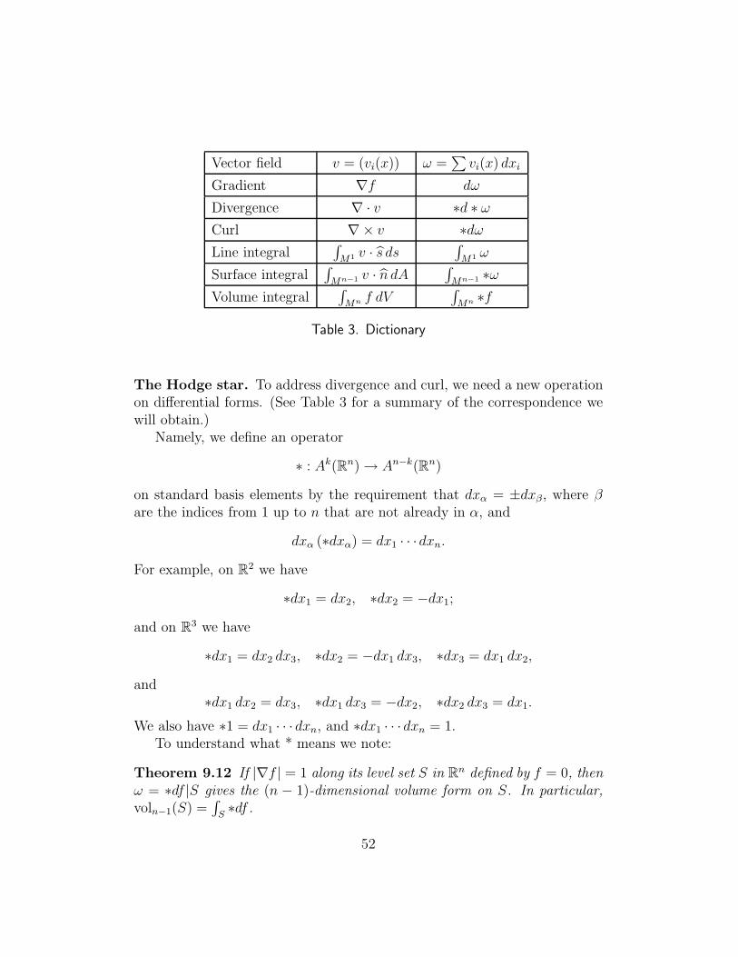
Vector field v = (vi(x)) ω =∑vi(x) dxi
Gradient ∇f dω
Divergence ∇ · v ∗d ∗ ωCurl ∇× v ∗dωLine integral
∫M1 v · s ds
∫M1 ω
Surface integral∫
Mn−1 v · n dA∫
Mn−1 ∗ωVolume integral
∫Mn f dV
∫Mn ∗f
Table 3. Dictionary
The Hodge star. To address divergence and curl, we need a new operationon differential forms. (See Table 3 for a summary of the correspondence wewill obtain.)
Namely, we define an operator
∗ : Ak(Rn) → An−k(Rn)
on standard basis elements by the requirement that dxα = ±dxβ, where βare the indices from 1 up to n that are not already in α, and
dxα (∗dxα) = dx1 · · ·dxn.
For example, on R2 we have
∗dx1 = dx2, ∗dx2 = −dx1;
and on R3 we have
∗dx1 = dx2 dx3, ∗dx2 = −dx1 dx3, ∗dx3 = dx1 dx2,
and∗dx1 dx2 = dx3, ∗dx1 dx3 = −dx2, ∗dx2 dx3 = dx1.
We also have ∗1 = dx1 · · · dxn, and ∗dx1 · · · dxn = 1.To understand what * means we note:
Theorem 9.12 If |∇f | = 1 along its level set S in Rn defined by f = 0, thenω = ∗df |S gives the (n − 1)-dimensional volume form on S. In particular,voln−1(S) =
∫S∗df .
52
More generally, for any oriented hypersurface S with unit normal n, wedefine
flux(v, S) =
∫
S
(n · v) |dA|,
and we have
flux(∇f, S) =
∫
S
∗df.
Divergence via forms. We now find that if v ⇐⇒ ω then
∇ · v ⇐⇒ ∗d ∗ ω.
Indeed, using the fact that dxj(∗dxi) = 0 if i 6= j, we have
d ∗ ω = d∑
vi ∗ dxi =∑
(dvi/dxi)dxi(∗dxi) = (∇ · v)dx1 · · · dxn.
One can now check that
flux(v, S) =
∫
S
(n · v) |dA| =
∫
S
∗ω.
This is because, for example, if S is the x − y plane in R3, then dx dy pullsback to the standard area form while dx dz and dy dz pull back to zero. Asa consequence we obtain the usual:
Theorem 9.13 (The divergence theorem) For any closed region U ⊂Rn with boundary S, and any vector field v, we have
∫
U
(∇ · v) |dV | =
∫
S
(n · v) |dA|.
Proof. Converting to the differential form ω ⇐⇒ v, this just says∫
Ud∗ω =∫
∂U∗ω.
Curl. Next we observe that curl in R2 or R3 satisfies, if v ⇐⇒ ω,
∇× v ⇐⇒ ∗dω.
Thus in R2,(∇× v)|dA| ⇐⇒ dω,
53
and in R3,n · (∇× v)|A| ⇐⇒ dω.
Notice how much simpler the formula becomes in terms of differential forms.For example, in R3 for v = (f, 0, 0), if we write fi = df/dxi, then we have
∗dω = ∗d(f dx1) = ∗(f2 dx2 + f3 dx3)dx1
= (−f2 dx3 + f3 dx2) ⇐⇒ (0, f3, f2)
in agreement with our previous formula for curl. Thus we have:
Theorem 9.14 (Green’s theorem) Any vector field v on a compact regionU ⊂ R2 with boundary S satisfies
∫
S
v · s |ds| =
∫
U
(∇× v) |dA|,
where s is a unit vector field tangent to the boundary.
Proof. This translates the statement∫
∂Uω =
∫Udω. Alternatively it can
be written: ∫
S
F dx+Gdy =
∫
U
(dG/dx− dF/dy) dx dy.
Corollary 9.15 We have v = ∇f locally iff ∇× v = 0.
Proof. If v = ∇f then ∇× v = 0 because d(df) = 0. Conversely, if dω = 0then
∫ x
aω = f(x) is locally well-defined and satisfies df = ω.
Thus our earlier result on H1(U) = 0 gives:
Theorem 9.16 A vector field v on a convex region U ⊂ Rn, n = 2, 3, canbe expressed as a gradient, v = ∇f if and only if ∇× v = 0.
In R3, Green’s theorem describes the integral of the curl over a curvilinearsurface U ⊂ R3:
54
Theorem 9.17 We have∫
∂S
v · s ds =
∫
S
n · (∇× v) |dA|.
All these results have a good conceptual explanation: div and curl mea-sure divergence and circulation around tiny loops or boxes, which assembleto give ∂U .
The Laplacian. The flow generated by a vector field is volume-preservingon Rn iff ∇ · v = 0. There are a multitude of such vector fields, but manyfewer if we require they have no circulation. That is, if add the conditionthat ∇×v = 0, then v = ∇f (at least locally), and we get Laplace’s equation:
∇ · ∇f = ∆f =∑ d2fi
dx2i
= 0.
This equation is of great importance in both mathematics and physics. Itssolutions are harmonic functions. They formally minimized
∫|∇f |2.
In electromagnetism, f is the potential of the electric field E = ∇f . Itsatisfies
∇E = ∆f = ρ
where ρ is the charge density. This ∆f = 0 is the equation for the electricpotential in a vacuum.
To find this potential when the boundary of a region U is held at fixedpotentials, one must solve Laplace’s’ equation with given boundary condi-tions.
Example: f(r) = 1/rn−2 is harmonic on Rn − 0 and represents thepotential of a point charge at the origin. The charge can be calculated interms of the flux through any sphere.
In terms of the Hodge star, we can write
∆f = ∗d ∗ df.
10 Elementary complex analysis
Relations of complex analysis to other fields include: algebraic geometry,complex manifolds, several complex variables, Lie groups and homogeneous
55
spaces (C,H, C), geometry (Platonic solids; hyperbolic geometry in dimen-sions two and three), Teichmuller theory, elliptic curves and algebraic numbertheory, ζ(s) and prime numbers, dynamics (iterated rational maps).
Complex algebra. Let C = R ⊕ Ri where i2 = −1. This set forms a fieldextension of R.
For z = x+ iy ∈ C we define z = x− iy. This is the Galois conjugate ofz; it uses the ‘other’ square-root of -1. Then
x = Re(z) = (z+z)/2, y = Im(z) = (z−z)/(2i), and x2+y2 = |z|2 = zz.
We use the metric d(z, w) = |z − w| to make C into a metric space.From this last expression we see how to invert complex numbers:
1/z = z/|z|2 = (x− iy)/(x2 + y2).
Complex multiplication as a matrix. Note that i acts on R2 by
J = ( 0 −11 0 ) .
Similarly T (z) = (x + iy)z is the linear map xI + yJ = ( x −yy x ). We thus
obtain an embedding C →M2(R), sending |z| = 1 to SO2(R).
Complex differentiation. Calculus with complex functions that are ex-pressed in terms of z and z is fairly simple. First note that
dz = x+ iy and dz = x− iy
are ordinary complex value differential forms. If we introduce the operators
d
dz=
1
2
(d
dx− i
d
dy
)and
d
dz=
1
2
(d
dx+ i
d
dy
),
then we have, for any smooth function f on a region in C,
df =df
dzdz +
df
dzd.
Complex analytic functions. A region U ⊂ C is an open, connected set.A function f : U → C is analytic if
f ′(z) = limt→0
f(z + t) − f(z)
t
56
exists for all z ∈ U . Note that t is allowed to approach 0 is any way whatso-ever. Equivalently we have
f(z + t) = f(z) + f ′(z)t+ o(|t|).The following are equivalent:
1. f is analytic: i.e. f ′(z) exists for all z.
2. f is differentiable on U and at each point, Df =(
a b−b a
)for some
a, b ∈ R.
3. Df is conformal (angle-preserving or zero), i.e. Df ∈ R · SO(2,R).
4. (Df)J = J(Df), where J = ( 0 −11 0 ).
5. f = u + iv and du/dx = dv/dy, du/dy = −dv/dx. (Cauchy-Riemannequations).
6. df/dz = 0.
If f(z) is analytic, then f ′(z) = df/dz.
Polynomials. To give some examples of analytic functions, let z = x + iyand z = x − iy. There is a natural isomorphism C[x, y] ∼= C[z, z] where z, zare formally treated as independent variables. Under this isomorphism, d/dzand d/dz behave as expected.
Thus a polynomial P (x, y) is analytic iff, when expressed in terms of zand z, it only involves z.
Theorem 10.1 (Fundamental theorem of algebra) Any polynomial P (z)of degree > 0 has a root in C, and hence can be factored as
P (z) = C(z − a1) · · · (z − ad).
We will shortly prove this using analysis. Here is a nice application, usinglogarithmic differentiation.
Theorem 10.2 The critical points of a polynomial P (z) are contained inthe convex hull of its zeros.
Proof. Suppose for example Re ai ≥ 0 for every zero ai of P . Note thatRew < 0 ⇐⇒ Re 1/w < 0. Thus ReP ′/P = Re
∑1/(z − ai) < 0 whenever
Re z < 0. This shows Re c ≥ 0 for any critical point of P , i.e. c lies in thesame halfplane as the zeros ai. Applying the same reasoning to P (eiθz) givesthe result above.
57
Example. Suppose P (z) has only one real zero a and one real critical pointb < a. Then P (z) must also have a complex zero with Re z ≤ b.
Rational functions. Suppose P,Q are polynomials, with Q 6= 0. We canthen form the quotient rational function
R(z) = P (z)/Q(z).
By canceling common zeros, we can assume P and Q have no common zero.Thus
R(z) = C∏
(z − ai)/∏
(z − bi).
This function has zeros at z = ai and poles at z = bi. If repeated, these zerosand poles have multiplicities.
Theorem 10.3 The space of rational functions forms a field C(z).
Note that when adding or multiplying rational functions, one must takecare to cancel common factors in the resulting fraction, to obtain R = P/Qwith gcd(P,Q) = 1. This is the same procedure as representing the rationalnumbers Q by ratios p/q of relatively prime integers.
Theorem 10.4 The degree of R(S(z)) is given by (degR)(deg S).
The Riemann sphere. We let C = C ∪ ∞ with the topology chosenso that |zn| → ∞ iff zn → ∞. Addition and multiplication continue to bewell-defined, except for ∞ + ∞ and ∞∗ 0. Assuming we write R = P/Q inlowest terms, then R(z) is well-defined at every point and gives a map
R : C → C.
The value R(∞) is determine by continuity. More precisely, R has a zeroat infinity of order e if e = deg(Q) − deg(P ) > 0, and pole of order e ife = deg(P ) − deg(Q) > 0. Otherwise R(∞) is finite and nonzero; it is thequotient of the leading coefficients of P and Q.
Degree. Assume P and Q have no common factor. Then we define thedegree of R by degR = max(degP, degQ).
Theorem 10.5 If deg(R) = d > 0, then for any p ∈ C the equation R(z) =p has exactly d solutions, counted with multiplicity.
58
Example. The function R(z) = z/(z3 + 1) has three zeros — one at z = 0,and one at z = ∞, the latter with multiplicity two.
Mobius transformations. A rational map of degree 1 gives a bijectionf : C → C whose inverse is also a rational function. Thus the set of suchMobius transformations form a group with respect to composition.
Mobius transformations send circles/lines to circles/lines. For example,the images of straight lines under z 7→ 1/z are circles tangent to the origin.The map
f(z) = iz + 1
z − 1
sends the unit disk to the upper half plane.
Theorem 10.6 There is a unique Mobius transformation sending any threegiven distinct points to any three others.
In particular, if f fixes 3 points then it is the identity.
Dynamics of Mobius transformations. Consider f(z) = 1/(z+1). Thenthe forward orbit of z = 0 is 1, 1/2, 2/3, 3/5, 5/8, 8/13, . . . which converges to
1/γ where γ is the golden ratio. In fact fn(z) → 1/γ for all z ∈ C, except forthe other fixed-point of f . (Which is at −γ.) To see this we just normalizeso the two fixed-point are 0 and infinity. Then f takes the form z 7→ λz, andin fact λ = f ′(1/γ) = −1/γ2.
These fixed points correspond to eigenvectors for A = ( 0 11 1 ) acting on C2.
Indeed, f(z) gives the slope of A(z, 1) in terms of the slope of (z, 1).
Power series. Let an ∈ C be a sequence with R = lim sup |an|1/n < ∞.Then f(z) =
∑anz
n converges for |z| < 1/R, and defines an analytic func-tion on this region with
f ′(z) =∑
nanzn−1.
This all follows by uniform convergence of functions and their derivatives.
Examples. The series ez =∑zn/n! gives an analytic function e : C → C∗.
From this we can obtain the functions sin(z), cos(z) and tan(z). By the usualalgebraic manipulations we find ez+w = ezew and in particular
ex+iy = exeiy.
In particular, f(z) = ez gives a surjective map f : C → C∗.
59
The series∑∞
0 zn = 1/(1−z) is only convergent for |z| < 1, but it admitsan analytic extension to C − 1 and then to a rational function.
Remarkably, the converse holds: any analytic function is locally a powerseries, and in particular the existence of one derivative implies the existenceof infinitely many.
Integrals along paths and boundaries of regions. Suppose f : U → C
is continuous. If γ : [0, 1] → C is a path or closed loop, we have
∫
γ
f(z) dz =
∫ 1
0
f(γ(t))γ′(t) dt.
Note: you can only integrate a 1-form, not a function!More geometrically, if we choose points zi close together along the loop
γ, then we have
∫
γ
f(z) dz = lim∑
f(zi)(zi+1 − zi).
This definition makes it clear and elementary that∫
γdz = 0 for any closed
loop γ. Note also that
∣∣∣∣
∫
∂U
f(z) dz
∣∣∣∣ ≤ (max∂U
|f(z)|) · length(∂U).
Cauchy’s Theorem. The most fundamental and remarkable tool in com-plex analysis is Cauchy’s theorem, which allows one to evaluate integralsalong loops or more generally boundaries of plane regions.
Theorem 10.7 Let U ⊂ C be a bounded region with piecewise-smooth bound-ary, and let f(z) be analytic on a neighborhood of U . Then
∫
∂U
f(z) dz = 0.
Provisional proof. Let us assume that f ′(z) is continuous. Then df =(df/dz) dz+(df/dz) dz; hence d(f dz) = 0, and the result follows from Stokes’theorem.
60
Simple cases: polynomials, power series. Note that if γ is a path from ato b then
∫γzn dz = (bn+1 − an+1)/(n+ 1). This proves that
∫∂UP (z) dz = 0
for any polynomial P . Taking limits, we find that the same is true for apower series f(z) =
∑an(z− p)n, so long as γ is contained within its radius
of convergence.
Cauchy’s integral formula. Because of Cauchy’s theorem, there is onlyone integral that needs to be explicitly evaluated in complex analysis:
∫
S1
dz
z=
∫
S1(a,r)
dz
z − a= 2πi.
From this we obtain:
Theorem 10.8 If f is analytic on U and continuous on U , then for allp ∈ U we have:
f(p) =1
2πi
∫
∂U
f(z) dz
z − p·
Corollary 10.9 More generally, we have
f (n)(p)
n!=
1
2πi
∫
∂U
f(z) dz
(z − p)n+1·
Corollary 10.10 All derivatives of f are analytic.
Corollary 10.11 All the derivatives of f exist, i.e. f is a C∞ function onU .
Consequences.
Theorem 10.12 If f(z) in analytic in B = B(p, R) and continuous onS1(p, R), then ∣∣∣∣
fn(p)
n!
∣∣∣∣ ≤ R−n max∂B
|f(z)|.
Corollary 10.13 The power series∑an(z − p)n, with an = f (n)(p)/n!, has
radius of convergence at least R.
Corollary 10.14 A bounded entire function is constant.
Corollary 10.15 Every nonconstant polynomial p(z) has a zero.
Proof. Otherwise 1/p(z) would be a bounded, nonconstant entire function.
61
Theorem 10.16 (Weierstrass-Casorati) If f : C → C is an entire func-tion, then f(C) is dense in C.
Proof. If B(p, r) does not meet f(C), then |1/(f(z)− p)| ≤ 1/r on all of C.
Corollary 10.17 An entire function with Re f(z) bounded above is constant.
Analytic functions from integrals. More generally, for any continuousfunction g on ∂U , the function
F (p) =
∫
∂U
g(z) dz
(z − p)m
is analytic in U ; indeed, it satisfies
F ′(p) = m
∫
∂U
g(z) dz
(z − p)m+1·
However it is only when g(z) is analytic that F provides a continuous exten-sion of g.
Goursat’s proof. We can now complete Cauchy’s theorem by proving: iff(z) is analytic then f ′(z) is continuous.
In fact we will show that if f(z) is analytic in a ball B(c, r) then F (p) =∫ p
cf(z) dz is well-defined and satisfies F ′(z) = f(z). Thus F is analytic with
a continuous derivative; and hence all its derivatives, including F ′′(z) = f ′(z),are continuous.
The key to the definition of F is to show that∫
∂Rf(z) dz = 0 for any
rectangle R. Suppose not. We may assume R has largest side of length1 and
∫∂Rf(z) dz = 1. Subdividing, we can obtain a sequence of similar
rectangles R = R0 ⊃ R1 ⊃ R2 . . . such that the largest side length of Rn is2−n and |
∫∂Rn
f(z) dz| ≥ 4−n. Suppose⋂Rn = p. Then on Rn we have
f(z) = f(p) + f ′(p)(z − p) + en(z), where |en| ≤ ǫn|z − p| and ǫn → 0. Nowthe first two terms have a zero integral over Rn, while the last term is, onRn, bounded by 2−nǫn. Moreover the length of ∂Rn is at most 4 · 2−n. Thus
∣∣∣∣
∫
Rn
f(z) dz
∣∣∣∣ ≤ 4ǫn4−n < 4−n
when n is large enough — a contradiction.
62
Taylor series. We can now show:
Theorem 10.18 Every analytic function is locally given by its Taylor series.
Proof. It suffices to treat the case where f(z) is analytic on a neighborhoodof B = B(0, 1). We first observe, by Cauchy’s bound, that
∑ fn(0)
n!pn
has radius of convergence at least 1. We will show that in fact it convergesto f(p).
Within B we can write
f(p) =1
2π
∫
∂B
f(z) dz
z − p·
Now we write, for z ∈ ∂B = S1,
1
z − p=
1
z(1 − p/z)=
1
z
∞∑
0
(p/z)n.
This power series converges uniformly on S1 for any fixed p ∈ B, since|p/z| = |p| < 1. Thus we can integral term-by-term to obtain
f(p) =∑
pn 1
2πi
∫
∂B
f(z) dz
zn+1=∑ fn(0)
n!pn·
When combined with Cauchy’s bound (Theorem 10.12) we obtain:
Theorem 10.19 If f(z) is analytic on B(0, R) then for all z in the ball wehave f(z) =
∑anz
n where an = f (n)(z)/n!. In particular, the Taylor seriesfor f at 0 has radius of convergence ≥ R.
Corollary 10.20 Any analytic function f(z) =∑anz
n has a singularity(where it cannot be analytically continued) on its circle of convergence |z| =R = 1/ lim sup |an|1/n.
63
Example. The power series 1/(1 + z2) = 1 − z2 + z4 − z6 + · · · has radiusof convergence R = 1 (even on the real axis). This shows z2 + 1 has a zeroon the circle |z| = 1 (even though it has no real zero).
Manipulation of Taylor series. Once one knows the power series for f(z)and g(z) , the power series for f(g(z)) and f(z)g(z) can easily be computedby formal manipulations (justified by the chain rule and product rule).
Example: we have exp(z2) =∑z2n/n!, and
exp(z)2 =(1 + z + z2/2 + z3/6 + · · ·
)2
= 1 + 2z + 2z2 + 4z3/3 + 2z4/3 + 4z5/15 + · · ·
Coefficients in Taylor series. We remark that it is very easy to understandwhere the integral formulas for the coefficients in f(z) =
∑anz
n comes from:namely
∫S1 z
n dz = 2πi when n = −1, and otherwise the integral is zero; thus
an =1
2πi
∫
S1
f(z) dz
zn+1·
Isolation of zeros. If f(z) =∑anz
n is not identically zero, then we canwrite it as f(z) = zn(
∑an−iz
i) = zng(z) where g(0) = an 6= 0. In this casewe say f has a zero of multiplicity n at z = 0. Also, by continuity, there isan r > 0 such that g(z) 6= 0 on B(0, r). This shows:
Theorem 10.21 Let f : U → C be an analytic function on a connecteddomain. Then either f is identically zero, or its zeros are isolated.
Proof. Let V ⊂ U be the set of points where f is locally zero. By definitionV is open, and by the argument above, it contains any non-isolated point ofthe zero set of f . This shows V is also closed. If f has a non-isolated zeroat p, then p ∈ V and then V = U by connectedness.
Example. The function f(z) = exp(2πi/z) satisfies f(1/n) = 0 for allintegers n. But it is not analytic at z = 0, so this is not a contradiction.(One can easily make smooth functions whose zeros sets are not isolated.)
Corollary 10.22 (Uniqueness of analytic continuation) If f and g areanalytic, and agree on a nonempty open subset of a region U (or more gen-erally on any set with a limit point on U), then f(z) = g(z) throughout U .
64
Corollary 10.23 If f is constant along an arc, then f is constant.
Theorem 10.24 Suppose fn(z) are analytic functions on U and fn → funiformly on compact sets. Then f(z) is also analytic.
Proof. For any p ∈ U we have
f(p) = lim fn(p) = lim1
2πi
∫
∂B(p,r)
fn(z)
z − pdz =
1
2πi
∫
∂U
f(z)
z − pdz,
by uniform convergence on B(p, r). As remarked earlier, this formula givea holomorphic function on B(p, r) no matter what the continuous functionf(z) on ∂B(p, r) is.
Theorem 10.25 Any bounded sequence of analytic functions fn ∈ C(U) hasa subsequence converging uniformly on compact sets to an analytic functiong.
Proof. If K ⊂ U and d(K, ∂U) = r, and |f | ≤ M , then for any p ∈ K wefind:
|f ′(p)| =1
2π
∣∣∣∣
∫
S1(p,r)
f(z)
(z − p)2dz
∣∣∣∣ ≤M/r.
Thus fn|K is equicontinuous and we can apply Arzela-Ascoli.
Note: a bounded function need not have a bounded derivative! Considerf(z) =
∑zn/n2 on the unit disk.
Theorem 10.26 If a sequence of analytic functions fn converges to f (lo-
cally) uniformly, then for each k, f(k)n (z) → fk(z) (locally) uniformly.
What happens with the usual suspects? All of these theorems havecounterexamples for functions of a real variable. For example, fn(x) = 1/(1+(nx)2) is bounded on the whole real axis, but it has no uniformly convergencesubsequence on [−1, 1].
What happens if we consider fn(z), z ∈ C? In this case fn(z) has apole at z = i/n. Thus it is not bounded in C, and not even bounded on auniform neighborhood of [−1, 1]. This explosion of |f(z)| is necessary to geta counterexample on [−1, 1].
Antiderivatives. A region U ⊂ C is simply-connected if every closed loopin U bounds a disk in U . Equivalently, C−U is connected (U has no holes).
65

Theorem 10.27 If f(z) is analytic on a simply-connect region U , then thereexists an analytic function F : U → C such that F ′(z) = f(z).
Corollary 10.28 If γ is any loop in a simply-connected region on which f(z)is analytic, then
∫γf(z) dz = 0.
Inverse functions. Observe that if Df is conformal and invertible, then(Df)−1 is also conformal. Thus the inverse function theorem already provedfor maps on Rn shows:
Theorem 10.29 If f is analytic and f(a) = b, then there is an analyticinverse function g defined near b such that g(b) = a and g′(b) = 1/f ′(a).
Log and roots. As first examples, we note that log(z) can be definednear z = exp(0) = 1 as an analytic function such that exp(log z) = z andlog 1 = 0. Similarly z1/n can be defined near z = 1, as the inverse of zn.More generally zα = exp(α log z) can be defined near z = 1.
To examine log more closely, let us try to define the function
F (p) =
∫ p
1
dz
z
on C∗. The problem is that the integral over a loop enclosing z = 0 is 2πi.Nevertheless, on any region U containing z = 1 where F can be defined, wehave F ′(z) = 1/z and F (1) = 0. Thus on U we have
(eF (z)
z
)′
=
(eF (z)(zF ′(z) − 1)
z2
)′
= 0
and thus eF (z) = z, i.e. F (z) = log z. A common convention is to takeU = C− (∞, 0]. Then F maps U to the strip | Im z| ≤ π. Explicitly, we have
log(z) = log |z| + i arg(z)
where the argument is chosen in (−π, π).By integration of (1 + z)−1 =
∑(−1)nzn we obtain the power series
log(1 + z) =
∫dz/(1 + z) = z − z2/2 + z3/3 − · · · ,
66
valid for |z| < 1.Once log z has been constructed we can then define zα on U as well. By
differentiation we then obtain the power series
(1 + z)α = 1 + αz +α(α− 1)
2!z2 +
α(α− 1)(α− 2)
3!z3 + · · · ,
also valid for |z| < 1.In both cases we have a branch-type singularity at z = 0 (not a pole! and
not an isolated singularity).
11 Analytic and harmonic functions
We begin by observing Cauchy’s theorem implies:
Theorem 11.1 (The mean-value formula) If f is analytic on B(p, r),then f(p) is the average of f(z) over S1(p, r).
Proof. By Cauchy’s integral formula, we have:
f(p) =1
2πi
∫ 2π
0
f(p+ reiθ)
reiθd(reiθ) =
1
2π
∫ 2π
0
f(p+ reiθ) dθ.
Corollary 11.2 (The Maximum Principle) A nonconstant analytic func-tion does not achieve its maximum. For example, if f is analytic on U andcontinuous on U , and U is compact, then
|f(z)| ≤ max∂U
|f(z)|.
Proof. If f(z) achieves its maximum at p ∈ U , then f(p) is the averageof f(z) over a small circle S1(p, r). Moreover, |f(z)| ≤ |f(p)| on this circle.The only way the average can agree is if f(z) = f(p) on S1(p, r). (Indeed,the average of g(z) = f(z)/f(p) is 1 and |g| ≤ 1 so g(z) = 1 on S1(p, r).)But then f is constant on an arc, so it is constant in U .
67
The Schwarz lemma. As a consequence of the maximum principle, we canprove a beautiful contraction property (that we will later formulate in termsof hyperbolic geometry).
Theorem 11.3 (Schwarz) Suppose f : ∆ → ∆ and f(0) = 0. Then forz 6= 0, |f(z)| ≤ |z|, and |f ′(0)| ≤ 1. If equality holds, then f(z) = eiθz.
Proof. Let f(z) =∑anz
n = a1z + · · · , and let F (z) =∑anz
n−1. ThenF (z) is analytic on ∆, F (z) = f(z)/z for z 6= 0 and F (0) = f ′(0). For|z| ≤ r we have |f(z)| ≤ 1/r by the maximum principle. Letting r → 1 gives|F (z)| ≤ 1. If F achieves this value inside the disk, it must be constant andhence f must be a rotation.
As an exercise one can use the Schwarz lemma to establish:
Corollary 11.4 If f(z) is analytic on ∆, f(0) = 0 and Re f ≤ 1, then| Im(f)| ≤ C(r) for all r < 1.
Note: f(z) = 2z/(z−1) maps ∆ onto R = z : Re z < 1, since f(0) = 0,f(−1) = 1 and f(1) = ∞. So Re f is bounded but Im f is not.
Corollary 11.5 Suppose fn : ∆ → C is a sequence of analytic functions withfn(0) = 0 such that Re fn converges uniformly on ∆. Then Im fn convergesuniformly on compact subsets of ∆.
Harmonic functions. A C2 real-value function u(z) is harmonic if
∆u =d2u
dx2+d2u
dy2= 4
d2
dz dz= 0.
Equivalently, we haved ∗ du = 0;
or, in terms better adapted to complex analysis,
4d2u
dz dz= ∆u = 0.
Theorem 11.6 If f = u+ iv is analytic, then u and v are harmonic.
68
Proof 1. By the Cauchy-Riemann equations, we have du/dx = dv/dy anddu/dy = −dv/dx, so
∆u =d2u
dx2+d2u
dy2=
d2v
dx dy− d2v
dy dx= 0.
Proof 2. The functions u and v are in the span of f and f , and sincedf/dz = 0 and df/dz = 0, we have ∆f = ∆f = 0.
Examples. The function Re(z3) = x3 − 3xy2 is a harmonic polynomial.The function Re(ez) = ex cos(y) is also harmonic. It might be hard to inventthese examples without using complex analysis.
Harmonic conjugates. A holomorphic function f is itself a (complex-valued) harmonic function. Conversely we have:
Theorem 11.7 If u is harmonic on a simply-connected region U , then thereis an analytic function f : U → C such that u(z) = Re f(z). Equivalently,there is a harmonic conjugate function v(z) such that u+ iv is analytic.
For example, u(z) = log |z| = Re log z is harmonic on C∗; its harmonicconjugate v(z) = arg(z) is however multivalued, even though u is single-valued.
Proof. Suppose u is harmonic. Then ω = du/dz dz is closed (dω = 0) andhence (since U is simply-connected), ω = df for some function f : U → C.But since
df =df
dzdz +
df
dzdz =
du
dzdz,
we have df/dz = 0 and hence f is holomorphic. Finally
d(f + f) =du
dzdz =
du
dzdz = du;
so, after adding a constant to f , we have u = f + f and hence u = Re(2f).Then v = Im(2f) is the harmonic conjugate of u.
Corollary 11.8 The level sets of u and v are orthogonal. Thus the area-preserving flow generated by ∇u follows the level sets of v, and vice-versa.
69
Corollary 11.9 Any C2 harmonic function is actually infinitely differen-tiable.
Corollary 11.10 A harmonic function satisfies the mean-value theorem:u(p) is the average of u(z) over S1(z, p).
Corollary 11.11 A harmonic function satisfies the maximum principle.
Corollary 11.12 If u is harmonic and f is analytic, then u f is alsoharmonic.
Theorem 11.13 A uniform limit of harmonic functions is harmonic.
Proof. Use Corollary 11.5 and the fact that a uniform limit of analyticfunctions is analytic.
Theorem 11.14 There is a unique linear map P : C(S1) → C(∆) such thatu = P (u)|S1 and u is harmonic on ∆.
Proof. Uniqueness is immediate from the maximum principle. To see ex-istence, observe that we must have P (zn) = zn and P (zn) = zn. Thus Pis well-defined on the span S of polynomials in z and z, and satisfies there‖P (u)‖∞ = ‖u‖∞. Thus P extends continuously to all of C(S1). Since theuniform limit of harmonic functions is harmonic, P (u) is harmonic for allu ∈ C(S1).
Poisson kernel. The map φ can be given explicit by the Poisson kernel.For example, u(0) is just the average of u over S1. We can also say u(p) isthe expected value of u(z) under a random walk starting at p that exits thedisk at z.
Relation to Fourier series. The above argument suggests that, to definethe harmonic extension of u, we should just write u(z) =
∑∞−∞ anz
n on S1,and then replace z−n by zn to get its extension to the disk. This actuallyworks, and gives another approach to the Poisson kernel.
Laplacian as a quadratic form, and physics. Suppose u, v ∈ C∞c (C)
– so u and v are smooth, real-valued functions vanishing outside a compactset. Then, by integration by parts, we have
∫
∆
〈∇u,∇v〉 = −∫
∆
〈u,∆v〉 = −∫
∆
〈v,∆u〉.
70
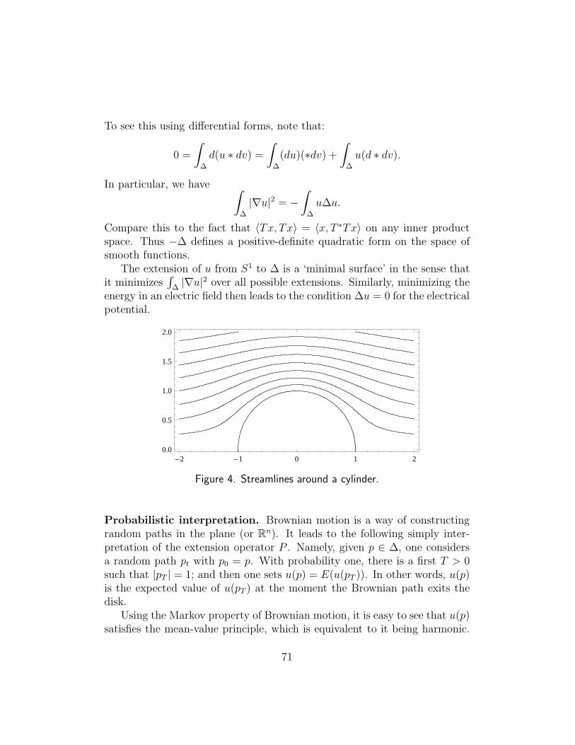
To see this using differential forms, note that:
0 =
∫
∆
d(u ∗ dv) =
∫
∆
(du)(∗dv) +
∫
∆
u(d ∗ dv).
In particular, we have ∫
∆
|∇u|2 = −∫
∆
u∆u.
Compare this to the fact that 〈Tx, Tx〉 = 〈x, T ∗Tx〉 on any inner productspace. Thus −∆ defines a positive-definite quadratic form on the space ofsmooth functions.
The extension of u from S1 to ∆ is a ‘minimal surface’ in the sense thatit minimizes
∫∆|∇u|2 over all possible extensions. Similarly, minimizing the
energy in an electric field then leads to the condition ∆u = 0 for the electricalpotential.
-2 -1 0 1 20.0
0.5
1.0
1.5
2.0
Figure 4. Streamlines around a cylinder.
Probabilistic interpretation. Brownian motion is a way of constructingrandom paths in the plane (or Rn). It leads to the following simply inter-pretation of the extension operator P . Namely, given p ∈ ∆, one considersa random path pt with p0 = p. With probability one, there is a first T > 0such that |pT | = 1; and then one sets u(p) = E(u(pT )). In other words, u(p)is the expected value of u(pT ) at the moment the Brownian path exits thedisk.
Using the Markov property of Brownian motion, it is easy to see that u(p)satisfies the mean-value principle, which is equivalent to it being harmonic.
71
It is also easy to argue that |p0 − pT | tends to be small when p0 is close toS1, and hence u(p) is a continuous extension of u|S1.
Example: fluid flow around a cylinder. We begin by noticing thatf(z) = z + 1/z gives a conformal map from the region U ⊂ H where |z| > 1to H itself, sending the circular arc to [−2, 2]. Thus the level sets of Im f =y(1 − 1/(x2 + y2)) describe fluid flow around a cylinder. Note that we aremodeling incompressible fluid flow with no rotation, i.e. we are assuming thecurl of the flow is zero. This insures the flow is given by the gradient of afunction.
Open mapping theorem. Next we explore the local form of an analyticfunction in more detail, to get a more informative understanding of the max-imum principle.
We remark that by the implicit function theorem we have:
Theorem 11.15 If f ′(z) 6= 0 then f is a local homeomorphism at z, and itsinverse is also analytic.
An integral formula for f−1 will be developed later, as a consequence ofRouche’s theorem. For the moment we note that the power series for f−1(z)is easily computed recursively from the power series for f(z). For example,if
f(z) = z + cos(z) − 1 = z − z2/2 + z4/24 + · · ·then f ′(0) = 1 and f−1(z) =
∑anz
n = z + a2z2 + a3z
3 + · · · where
z = f(∑
anzn)
= z + a2z2 + a3z
3 − (z + a2z2)2/2 + z4 +O(z4)
= z + (a2 − 1/2)z2 + (a3 − a2)z3 + · · · ,
which gives a2 = a3 = 1/2.
Theorem 11.16 If f(z) has an isolated zero at z = a, then there is ananalytic function g(z) defined near 0 such that g′(0) 6= 0 and f(z) = g(z)n
near z = a.
Proof. We can assume a = 0. Write f(z) = Aznh(z) with h(0) = 1, andset g(z) = zA1/nh(z)1/n. This makes sense when z is small, since z1/n =exp((log z)/n) is analytic near h(0) = 1.
72
Corollary 11.17 A nonconstant analytic function is open; that is, f(U) isopen whenever U is open.
This gives an alternative proof of the maximum principle.
Roots and logs. Note that for any α ∈ C, (1 + z)α = exp(α log(1 + z)) isanalytic near z = 0; in fact, it has a power series with radius of convergenceone, given by the binomial theorem:
(1 + z)α =
∞∑
0
αk
z
k
= 1 + αz +α(α− 1)
2!z2 +
α(α− 1)(α− 2)
3!z3 + · · · ;
thus by composition we have:
Lemma 11.18 If f(z) is analytic near z = 0 and f(0) 6= 0, then f(z)α isalso analytic near z = 0.
This result was used in the proof above.
12 Zeros and poles
Laurent series. As a complement to the Taylor series we have:
Theorem 12.1 (Laurent series) If f(z) is analytic in the region R1 <|z| < R2, then we can write
f(z) =
∞∑
−∞anz
n.
The terms with n > 0 give a power series that converges absolutely for |z| <R2, and the negative terms one that converges absolutely for |z| > R1.
Proof. Shrinking the annulus slightly, we may assume f is continuous on|z| = R1 and |z| = R2. Then we can write
f(p) =1
2πi
∫
S1(R2)
f(z) dz
z − p+
1
2πi
∫
S1(R1)
f(z) dz
p− z·
On the outside circle we have 1/(1−p/z) =∑
(p/z)n and on the inside circlewe have 1/(1 − z/p) =
∑(z/p)n. This gives the desired result with
an =1
2πi
∫
S1(r)
f(z) dz
zn+1
for any circle with R1 < r < R2.
73
Corollary 12.2 Any analytic function on r < |z| < R can be written as thesum of a function analytic for |z| < R and a function analytic for |z| > r.
Singularities and removability. Next we examine singularities moreclosely. Suppose f(z) is analytic on ∆∗ = ∆ − 0. Write f(z) =
∑anz
n ina Laurent series. Let N be the least n such that an 6= 0. Then we have thefollowing possibilities:
1. N = ∞: then f(z) = 0.
2. 0 < N <∞; then f(z) = zN (aN + · · · ) has an isolated zero of order Nat z = 0.
3. N = 0: then f(0) = aN 6= 0.
4. −∞ < N < 0: then f(z) = (aN/zN ) + · · · has a pole of order N at
z = 0, and |f(z)| → ∞ as z → 0.
5. N = −∞: then f(z) has an essential singularity at z = 0, and by ageneralization of the Weierstrass-Casorati theorem (see below), for any
p ∈ C there exist zn → 0 such that f(zn) → p.
In the first three cases, f has a removable singularity at z = 0. The mapf : ∆∗ → C has a continuous extension at z = 0 except in the last case.
Here is a maximum-type principle for a function with an isolated singu-larity.
Theorem 12.3 If f(z) is bounded on ∆∗, then z = 0 is a removable singu-larity; that is, f extends to an analytic function on ∆.
Proof. We may assume f is continuous on S1. Consider the function F (p) =(1/2πi)
∫S1 f(z)/(z− p) dz. This is analytic on ∆, since we may differentiate
with respect to p under the integral. On the other hand, by Cauchy’s formulawe have, for any r with 0 < r < |p|,
f(p) = F (p) − 1
2πi
∫
S1(r)
f(z) dz
z − p·
As r → 0, the integrand remains bounded while the length of S1(r) goes tozero, so we conclude that f(p) = F (p).
74
Corollary 12.4 The values of an analytic function are dense in any neigh-borhood of an essential singularity.
Proof. If B(p, r) is omitted from f(∆∗), then g(z) = 1/(f(z)−p) is boundednear 0 and hence analytic. Thus f(z) = p+1/g(z) has at worst a pole (whicharises if g(0) = 0).
Picard’s theorems. Picard’s little and big theorems show more: an entirefunction can have only one omitted value (and this is sharp for ez), and ananalytic function omits at most one value in any neighborhood of an essentialsingularity.
Corollary 12.5 Any analytic function on ∆∗ has the form f(z) =∑∞
−∞ anzn.
The number of negative terms is infinite iff f(z) has an essential singularityat z = 0.
Example. On ∆∗ the function e1/z =∑∞
0 z−n/n! has an essential singularityat z = 0. So does sin(1/z), etc.
Polynomials and rational functions.
Theorem 12.6 If f(z) is an entire function and |f(z)| ≤M |z|n, then f(z)is a polynomial of degree at most n.
Proof. By Cauchy’s bound, f (n)(z) is bounded and hence constant.
Theorem 12.7 If f(z) is entire and continuous at ∞, then f(z) is a poly-nomial.
Proof. In this case f(1/z) has at worst a pole at the origin, and so it satisfiesa bound as above.
Let us say a function f : C → C is holomorphic if whenever w = f(z), ifw, z ∈ C then f(z) is analytic; if w = ∞, z ∈ C then 1/f(z) is analytic; ifw ∈ C and z = ∞ then f(1/z) is analytic; and if w = z = p then 1/f(1/z)is analytic. (This is an example of a map between Riemann surfaces.)
Corollary 12.8 Any holomorphic function f : C → C is a rational function.
Proof. By compactness and isolation, 1/f(z) has only a finite number of
zeros in C, and hence only finitely many in C. Thus we can find a polynomialsuch that Q(z) = f(z)P (z) is analytic and continuous at infinity. Then Q(z)is also a polynomial.
75
13 Residues: theory and applications
Meromorphic functions. A function f : U → C is meromorphic if it isanalytic apart from a discrete set of poles. For example, 1/ sin(z) is mero-morphic.
In this section we analyze integrals of meromorphic functions over closedloops.
The residue. Let f(z) be a holomorphic function with an isolated singu-larity at p. The residue of f at p, Res(f, p), can be defined in two equivalentways:
1. Expand f in a Laurent series∑an(z − p)n; then a−1, the coefficient
of 1/(z − p), is the residue of f at p.2. Define Res(f, p) =
∫γf(z) dz for any small loop around p.
The second definition reveals that it is really the 1-form f(z) dz, not thefunction f(z), which has a residue. For example, we do not have Res(f(g(z)), p) =Res(f(z), g(p))! Instead — if g′(p) 6= 0 — we have
Res(f(g(z)), p) = g′(p) Res(f, g(p)).
Examples: simple poles. If f(z) has a simple pole at p, then
Res(f, p) = limz→p
f(z)(z − p).
Put differently: if f(z) has a simple zero at p, then
Res(1/f(z), p) = 1/f ′(p).
For example, Res(1/(z2 + 1), i) = 1/(2i) = −i/2. If f(z) has a simple poleat p and g(z) is analytic at p, then
Res(fg, p) = g(p) Res(f, p).
If f(z) vanishes to order exactly k at p, and g(z) to order (k + 1), then f/ghas a simple pole and we have
Res(f/g, p) = (k + 1)f (k)(p)
g(k+1)(p)·
This is immediate by writing, e.g. when p = 0, f(z) = zk(ak + O(z)) andg(z) = zk+1(bk+1 +O(z)). For example, Res(z2/(sin z − z), 0) = −6.
76
Logarithmic derivatives. If f(z) has a zero of order k at p then f ′/f hasa simple pole at p and we have
Res(f ′/f, p) = k.
Similarly if f has a pole of order k, then Res(f ′/f, p) = −k.Higher order poles. It is trickier to find the residue when the pole is notsimple. For example, Res(z3 cos(1/z), 0) = 1/24.
Integrals. The importance of residues comes from:
Theorem 13.1 (The residue theorem) Let U be a compact, smoothly boundedregion, suppose P ⊂ U is a finite set, and suppose f : U − P → C is contin-uous and analytic on U . Then we have
1
2πi
∫
∂U
f(z) dz =∑
P
Res(f, p).
Proof. Immediate by removing from U a small disk around each point P ,and then integrating along the boundary of the resulting region.
Note: if f(z) is analytic, then Res(f(z)/(z− p), p) = f(p), so the residuetheorem contains Cauchy’s formula for f(p).
Corollary 13.2 (The argument principle) Suppose f |∂U has no zeros.Then the number of zeros of f(z) inside U is given by
N(f, 0) =1
2π
∫
∂U
f ′(z) dz
f(z)·
This integral is the same as (1/2πi)∫
∂Ud log f . It just measure the number
of times that f wraps the boundary around zero.The topological nature of the argument principle: if a continuous f : ∆ →
C has nonzero winding number on the circle, then f has a zero in the disk.Letting N(f, a) denote the number of solutions to f(z) = a, we have
another proof of:
Corollary 13.3 (Open mapping theorem) The function N(f, a) is con-stant on each component of C− f(∂U). (It simply gives the number of timesthat f(∂U) winds around a.)
77
Corollary 13.4 A nonconstant analytic function is open.
Proof. Suppose f(p) = q. Choose a small ball B around p such thatq 6∈ f(∂B). Then f(B) hits all the points in the component of C − f(∂B)containing q.
Note that this argument relates the openness of f to the isolation of itszeros.
Theorem 13.5 (Rouche’s Theorem) If f and g are analytic on U and|g(z)| < |f(z)| on ∂U , then f(z) and (f + g)(z) have the same number ofzeros in U .
Proof. The function N(f + tg, 0) is continuous for t ∈ [0, 1], since f + tgnever vanishes on ∂U .
Corollary 13.6 (Fundamental theorem of algebra) Every nonconstantpolynomial p(z) has a n zeros in C.
Proof. Write p(z) = a0zn + g(z) = f(z) + g(z) where a0 6= 0 and deg g ≤
n − 1. Then |f | > |g| for z large, so p(z) has the same number of zeros aszn.
Example: zeros. We claim ez = 3zn has n solutions inside the unit circle.This is because |ez| ≤ e < 3 = |3zn| on S1.
Example: injectivity. If f(z) = z + g(z), where |g′(z)| < 1 on ∆, thenf |∆ is 1 − 1.
Proof. Given p ∈ ∆, we wish to show f(z) − f(p) = (z − p) + g(z) − g(p)has only one zero in the unit disk. Since z − p has exactly one zero in ∆,it suffices to show |g(z) − g(p)| < |z − p| on S1, which in turn follows from|g′| < 1.
Nonexample. The function f(z) = z4 is not 1-1 on B(1, 1) even though f ′
is nonzero through this region. The largest ball about z = 1 on which f isinjective has radius 1/
√2. The borderline case arises when z± = (1± i)/
√2,
which satisfies f(z−) = f(z+) = −1.Similarly, p(z) = z4 + 1 has two zeros in B(1, 1), even though p′(z) is
never zero in this region!
78
The fallacy that f ′ must vanish is absurdly common — doubtlessan effect of too steady a diet of algebraic function-theory, in whichall sheets of the Riemann surfaces are alike and extend over thewhole plane.
—Littlewood, A Mathematician’s Miscellany, p. 62.
Theorem 13.7 (Hurwitz) If fn(z) → g(z) locally uniformly, g is noncon-stant and g(p) = 0, then here are pn → p such that fn(pn) = 0 for all n≫ 0.
Proof. Choose a small r > 0 such that g|S1(p, r) has no zeros. Then|g| > m > 0 on S1(p, r). Once n is large enough, |fn − g| < m on S1(p, r), sofn also has a zero pn with |pn − p| < r. Now diagonalize.
Theorem 13.8 Let fn : U → C be a sequence of injective analytic functionsconverging uniformly to f . Then either f is constant or f is also injective.
Proof. Suppose f is not constant and f(a) = f(b) for some a 6= b. Thenz = a is an isolated zero of the nonconstant function g(z) = f(b)−f(z). Nowg itself is a uniform limit of gn(z) = fn(b) − fn(z), so by Hurwitz theoremthere are zn → a such that gn(zn) = 0. But this means fn(b) = fn(zn), andzn 6= b for n≫ 0.
The inverse function. Suppose f(p) = q and f ′(p) 6= 0. Then for a smallenough r, the locus T = f(S1(p, r)) is a circle winding once around f(p). Lets = d(p, T ); then for all w ∈ B(q, s) we have:
f−1(w) =1
2πi
∫
S1(p,r)
zf ′(z) dz
f(z) − w·
It also possible to use a power series for f(z) to give, directly, a powerseries for f−1(z). For example,
w = tan−1(z) = z − z3/3 + z5/5 − z7/7 + · · ·gives
z = w + z3/3 − z5/5 + z7/7 − · · ·= w +O(w3)
= w + w3/3 +O(w5)
= w + (w + w3/3)3/3 − w5/5 +O(w7)
= w + w3/3 + w5(1/3 − 1/5) +O(w7)
= w + w3/3 + 2w5/15 + 17w7/315 + ·
79
Definite integrals 1: rational functions on R. Whenever a rationalfunction R(x) = P (x)/Q(x) has
∫R|R(x)| dx is finite, we can compute this
integral via residues: we have∫ ∞
−∞R(x) dx = 2πi
∑
Im p>0
Res(R, p).
(Of course we can also compute this integral by factoring Q(x) and usingpartial fractions and trig subsitutions.)
Example. Where does π come from? It emerges naturally from rationalfunctions by integration — i.e. it is a period. Namely, we have
∫ ∞
−∞
dx
1 + x2= 2πiRes(1/(1 + z2), i) = 2πi(−i/2) = π.
Of course this can also be done using the fact that∫dx/(1+x2) = tan−1(x).
More magically, for f(z) = 1/(1 + z4) we find:∫ ∞
−∞
dx
1 + x4= 2πi(Res(f, (1 + i)/
√2) + Res(f, (1 + i)/
√2) =
π√2·
Both are obtain by closing a large interval [−R,R] with a circular arc in theupper halfplane, and then taking the limit as R → ∞.
We can even compute the general case, f(z) = 1/(1 + zn), with n even.For this let ζk = exp(2πi/k), so f(ζ2n) = 0. Let P be the union of the paths[0,∞)ζn and [0,∞), oriented so P moves positively on the real axis. We canthen integrate over the boundary of this pie-slice to obtain:
(1 − ζn)
∫ ∞
0
dx
1 + xn=
∫
P
f(z) dz = 2πiRes(f, ζ2n) = 2πi/(nζn−12n ),
which gives ∫ ∞
0
dx
1 + xn=
2πi
n(−ζ−12n + ζ+1
2n )=
π/n
sin π/n·
Here we have used the fact that ζn2n = −1. Note that the integral tends to 1
as n→ ∞, since 1/(1 + xn) converges to the indicator function of [0, 1].
Definite integrals 2: rational functions of sin(θ) and cos(θ). Hereis an even more straightforward application of the residue theorem: for anyrational function R(x, y), we can evaluate
∫ 2π
0
R(sin θ, cos θ) dθ.
80
The method is simple: set z = eiθ and convert this to an integral of ananalytic function over the unit circle. To do this we simple observe thatcos θ = (z + 1/z)/2, sin θ = (z − 1/z)/(2i), and dz = iz dθ. Thus we have:
∫ 2π
0
R(sin θ, cos θ) dθ =
∫
S1
R
(1
2i
(z − 1
z
),1
2
(z +
1
z
))dz
iz·
For example, for 0 < a < 1 we have:∫ 2π
0
dθ
1 + a2 − 2a cos θ=
∫
S1
i dz
(z − a)(az − 1)= 2πi(i/(a2 − 1)) =
2π
1 − a2·
Definite integrals 3: fractional powers of x.∫∞0xaR(x)dx, 0 < a < 1,
R a rational function.For example, consider
I(a) =
∫ ∞
0
xa
1 + x2dx.
Let f(z) = za/(1 + z2). We integrate out along [0,∞) then around a largecircle and then back along [0,∞). The last part gets shifted by analyticcontinuation of xa and we find
(1 − 1a)I(a) = 2πi(Res(f, i) + Res(f,−i))and Res(f, i) = ia/(2i), Res(f,−i) = (−i)a/(−2i). Thus, if we let ia = ω =exp(πia/2), we have
I(a) =π(ia − (−i)a)
(1 − 1a)= π
ω − ω3
1 − ω4=
π
ω + ω−1=
π
2 cos(πa/2)·
For example, when a = 1/3 we get
I(a) = π/(2 cos(π/6)) = π/√
3.
Residues and infinite sums. The periodic function f(z) = π cot(πz) hasthe following convenient properties: (i) It has residues 1 at all the integers;and (ii) it remains bounded as Im z → ∞. From these facts we can deducesome remarkable properties: by integrating over a large rectangle S(R), wefind for k ≥ 2 even,
0 = limR→∞
1
2πi
∫
S(R)
f(z) dz
zk= Res(f(z)/zk, 0) + 2
∞∑
1
1/nk.
81
Thus we can evaluate the sum∑
1/n2 using the Laurent series
cot(z) =cos(z)
sin(z)=
1 − z2/2! + z4/4! − · · ·z(1 − z2/3! + z4/5! − · · · )
= z−1(1 − z2/2! + z4/4! − · · · )(1 + z2/6 + 7z4/360 + · · · )= z−1 − z/3 − z3/45 − · · ·
(using the fact that (1/(3!)2 − 1/5! = 7/360). This shows Res(f(z)/z2, 0) =−π2/3 and hence
∑1/n2 = π2/6. Similarly, 2ζ(2k) = −Res(f(z)/z2k, 0).
For example, this justifies ζ(0) = 1 + 1 + 1 + · · · = −1/2.Little is known about ζ(2k + 1). Apery showed that Z(3) is irrational,
but it is believed to be transcendental.We note that ζ(s) =
∑1/ns is analytic for Re s > 1 and extends an-
alytically to C − 1 (with a simple pole at s = 1). In particular ζ(0) iswell-defined. Because of the factorization ζ(z) =
∏(1 − 1/ps)−1, the be-
havior of the zeta function is closely related to the distribution of primenumbers. The famous Riemann hypothesis states that any zero of ζ(s) with0 < Re s < 1 satisfies Re s = 1/2. It implies a sharp form of the primenumber theorem, π(x) = x/ log x+O(x1/2+ǫ).
The zeta function also has trivial zeros at s = −2,−4,−6, . . ..
Hardy’s paper on∫
sin(x)/x dx. We claim
I =
∫ ∞
0
sin x dx
x=π
2·
Note that this integral is improper, i.e. it does not converge absolutely. Also,the function f(z) = sin(z)/z has no poles — so how can we apply the residuecalculus?
The trick is to observe that
−2iI = limr→0
∫
r<|x|<1/r
eix dx
x·
We now use the fact that |eix+iy| ≤ e−y to close the path in the upperhalfplane, and conclude that
2iI = limr→0
∫
S1(r)+
eiz dz
z·
Since Res(eiz/z, 0) = 1, we find 2iI = (2πi)(1/2) and hence I = π/2.
82
14 Geometric function theory
Riemann surfaces. A deep theorem proved at the end of the 19th centuryis:
Theorem 14.1 Every simply-connect Riemann surface is isomorphic to C,C or ∆.
We will investigate these Riemann surfaces verify the theorem above forsimply– and doubly–connected regions in the plane.
Metrics. A conformal metric on a region U in C (or on a Riemann surface)is given by a continuous function ρ(z) |dz|. The length of an arc in U isdefined by
L(γ, ρ) =
∫ b
a
ρ(γ(t))|γ′(t)| dt,
and the area of U is defined by
A(U, ρ) =
∫
U
ρ(z)2 |dz|2.
If f : U → V is analytic, then
σ = f ∗(ρ) = ρ(f(z))|f ′(z)| |dz|.
By the change of variables formula, L(γ, f ∗σ) = L(f γ, ρ).1. The complex plane.
Theorem 14.2 Aut(C) = az + b : a ∈ C∗, b ∈ C.
Note that this is a solvable group, in fact a semidirect product.The usual Euclidean metric on C is given by |dz|. The subgroup of
isometries for this metric is the group of translations, C ⊂ Aut(C).Thus C itself is a group. What is the quotient C/Z?
Theorem 14.3 The map f(z) = exp(z) gives an isomorphism between C/(2πiZ)and C∗.
The induced metric on C∗ is ρ = |dz|/|z|. That is, f ∗ρ = |dz|. Thismetric makes C∗ into an infinite cylinder of radius 1.
2. The Riemann sphere. The map φ(z) = 1/z gives a chart near infinity.
83
Theorem 14.4 Aut(C) ∼= PSL2(C).
A particularly nice realization of this action is as the projectivization of thelinear action on C2.
The automorphisms of C act triply-transitively, and send circles to circles.(Proof of last: a circle x2+y2+Ax+By+C = 0 is also given by r2+r(A cos θ+B sin θ)+C = 0, and it is easy to transform the latter under z 7→ 1/z, whichreplaces r by 1/ρ and θ by −θ.) Stereographic projection preserves circlesand angles. Proof for angles: given an angle on the sphere, construct a pairof circles through the north pole meeting at that angle. These circles meet inthe same angle at the pole; on the other hand, each circle is the intersectionof the sphere with a plane. These planes meet C in the same angle they meeta plane tangent to the sphere at the north pole, QED.
The Mobius transformation represented by A ∈ PSL2(C) can be classifiedaccording to tr(A), which is well-defined up to sign. Any Mobius transfor-mation is either:
1. The identity, with tr(A) = ±2;
2. Parabolic (a single fixed point), with tr(A) = ±2;
3. Elliptic (conjugate to a rotation), with tr(A) = 2 cos θ ∈ (−2, 2); or
4. Hyperbolic (with attracting and repelling fixed points), with tr(A) =λ+ λ−1 ∈ C − [−2, 2].
Four views of C: the extended complex plane; the Riemann sphere; theRiemann surface obtained by gluing together two disks with z 7→ 1/z; theprojective plane for C2.
Spherical geometry. The spherical metric 2|dz|/(1 + |z|2). How to viewthis metric:
1. Derive from the fact “Riemann circle” and the map x = tan(θ/2), andconformality of stereographic projection. Note that 2dx = sec2(θ/2) dθ =(1 + x2) dθ, and thus |dθ| = 2|dx|/(1 + |x|2).
2. Alternatively, note that z 7→ eiθz and z 7→ 1/z generate the group ofrotations of the Riemann sphere, and leave this metric invariant.
84
3. Or, regarding C as PC2, define the length of w at v to be ‖w‖ =2|v∧w|/|v|2. Then if we map C into C2 by z 7→ (1, z), we get v = (1, z),w = (0, dz), and ‖w‖ = 2|dz|/(1 + |z|2).
In the last version we have used the Hermitian structure on C2. Note thatorthogonal vectors in C2 determine antipodal points in C.
Topology. Some topology of projective spaces: RP2 is the union of a diskand a Mobius band; the Hopf map S3 → S2 is part of the natural projectionC2 − 0 → C.
Gauss-Bonnet for spherical triangles: area equals angle defect. Proveby looking at the three lunes (of area 4θ) for the three angles of a triangle.General form: 2πχ(X) =
∫XK +
∫∂Xk.
Isometries. The isometry group of (C, ρ) is PU(2) ⊂ PSL2(C). Every finite
subgroup of Aut(C) is conjugate into PU(2). Thus the finite subgroups areZ/n, D2n, A4, S4 and A5.
3. The unit disk. We first remark that ∆ ∼= H, e.g. by the Mobiustransformation I(z) = i(1 − z)/(1 + z). Thus Aut(∆) ∼= Aut(H).
Theorem 14.5 Every automorphism of ∆ or H extends to an automorphismof C.
Proof. Let G(H) = Aut(H) ∩ Aut(C) and similarly for G(∆). Note that
I ∈ Aut(C) so G(∆) ∼= G(H) under I. Now G(H) obvious contains thetransformations of the form g(z) = az + b with a > 0, b ∈ R, which acttransitively. So G(∆) also acts transitively. Thus if f ∈ Aut(∆) then f(0) =0 after composition with an element of G(∆). But then f(z) = eiθz by theSchwarz Lemma, so f ∈ G(∆).
Corollary 14.6 The automorphism group of ∆ is PU(1, 1), the group ofMobius transformations of the form
g(z) =az + b
bz + a
with |a|2 − |b|2 = 1.
Corollary 14.7 The automorphism group of H is given by PSL2(R).
85
These automorphisms preserve the hyperbolic metrics on ∆ and H, givenby
ρ∆ =2|dz|
1 − |z|2 and ρH =|dz|Im z
·
Hyperbolic geometry. Geodesics are circles perpendicular to the circle atinfinity. Euclid’s fifth postulate (given a line and a point not on the line,there is a unique parallel through the point. Here two lines are parallel ifthey are disjoint.)
Gauss-Bonnet in hyperbolic geometry. (a) Area of an ideal triangle is∫ 1
−1
∫∞√1−x2(1/y
2)dydx = π. (b) Area A(θ) of a triangle with two ideal verticesand one external angle θ is additive (A(α+ β) = A(α) +A(β)) as a diagramshows. Thus A(α) = α. (c) Finally one can extend the edges of a generaltriangle T in a spiral fashion to obtain an ideal triangle containing T and 3other triangles, each with 2 ideal vertices.
Classification of automorphisms of H2, according to translation distance.
The Schwarz lemma revisited.
Theorem 14.8 Any holomorphic map f : H → H is a weak contraction forthe hyperbolic metric. If |Df | = 1 at one point, then f is an isometry.
Dynamical application of Schwarz Lemma.
Theorem 14.9 Let f : C → C be a rational map. Then the immediate basinof any attracting cycle contains a critical point.
Corollary 14.10 The map f has at most 2d− 2 attracting cycles.
Conformal mapping. Examples:
1. Mobius transformations. Lunes and tangent-lunes = pie-slices andstrips.
2. All pie-slices are isomorphic to H using zα.
3. All strips are isomorphic to H using exp.
4. A half-strip is isomorphic to a lune using exp, and hence to a half-plane.
5. Putting it all together: sin(z) maps the region above [−π/2, π/2] to H.
86
The Riemann mapping theorem.
Theorem 14.11 For any simply-connected region U ⊂ C, U 6= C, and anybasepoint u ∈ U , there is a unique conformal homeomorphism f : (U, u) →(∆, 0) such that f ′(u) > 0.
Proof. let F be the family of univalent maps (U, u) → (∆, 0). Using asquare-root and an inversion, show F is nonempty. Also F is closed underlimits. By the Schwarz Lemma, |f ′(u)| has a finite maximum over all f ∈ F .Let f be a maximizing function. If f is not surjective to the disk, then wecan apply a suitable composition of a square-root and two automorphismsof the disk to get a g ∈ F with |g′(u)| > |f ′(u)|, again using the SchwarzLemma.
Uniformization of annuli.
Theorem 14.12 Any doubly-connected region in the sphere is conformal iso-morphic to C∗, ∆∗ or A(R) = z : 1 < |z| < R.
The map from H to A(R) is z 7→ zα, where α = log(R)/(πi). The decktransformation is given by z 7→ λz, where λ = 4π2/ log(R).
Reflection. The Schwarz reflection principle: if U = U∗, and f is analyticon U ∩ H, continuous and real on the boundary, then f(z) extends f to allof U . This is easy from Morera’s theorem. A better version only requiresthat Im(f) → 0 at the real axis, and can be formulated in terms of harmonicfunctions (cf. Ahlfors):
If v is harmonic on U∩H and vanishes on the real axis, then v(z) = −v(z)extends v to a harmonic function on U . For the proof, use the Poisson integralto replace v with a harmonic function on any disk centered on the real axis;the result coincides with v on the boundary of the disk and on the diameter(where it vanishes by symmetry), so by the maximum principle it is v.
Reflection gives another proof that all automorphisms of the disk extendto the sphere.
Univalent functions. The class S of univalent maps f : ∆ → C such thatf(0) = 0 and f ′(0) = 1. Compactness of S. The Bieberbach Conjecture/deBrange Theorem: f(z) =
∑anz
n with |an| ≤ n.The area theorem: if f(z) = z +
∑bn/zn is univalent on z : |z| > 1,
then∑n|bn|2 < 1. The proof is by integrating fdf over the unit circle and
87
observing that the result is proportional to the area of the complement ofthe image of f .
Solving the cubic and Chebyshev polynomials. Complex algebra findsits origins in the work of Cardano et al on solving cubic polynomial equations.Remarkably, complex numbers intervene even when the root to be found isreal.
One can always make a simple transformation of the form x 7→ x + c toreduce to the form
x3 + ax+ b = 0.
One can further replace x with cx to reduce to the form
x3 − 3x = b.
Thus the solution to the cubic involves inverting a single cubic functionP3(z) = z3 − 3z.
We have chosen this simple form for a reason. Namely, there is a sequenceof polynomials P1(z) = z, P2(z) = z2 − 2, P3(z) = z3 − 3z, etc. satisfying
Pn(z + 1/z) = (z + 1/z)n.
In other words, π(z) = z + 1/z gives the quotient of the Riemann sphereby z 7→ 1/z; since this map commutes with zn, the map Sn(z) = zn mustdescends to a polynomial on the quotient, satisfying
Pn(π(z)) = π(Sn(z)).
This polynomial is related to multiple angle formulas for cosine, since forz = eiθ we have π(z) = 2 cos θ, and thus:
Pn(2 cos θ) = 2 cos(nθ).
The map π is important in conformal mapping, e.g. it is what we used todescribe fluid flow around a cylinder.
In any case, to solve Pn(x) = a, we just write a = y + 1/y (by solving aquadratic equation), and then we have x = y1/n + y−1/n. In particular, thismethod can be used to solve x3 − 3x = a.
Example. To solve x3 = x + 1, we change variable by x = ay to obtainy3 − y/a2 = 1/a3. Setting a = 3−1/2, we just need to solve
y3 − 3y = 3√
3.
88

This is done by first writing 3√
3 = u+1/u, which gives u = (3√
3+√
23)/2,1/u = (3
√3−
√23)/2. Then we take a cube root v of u, and the final solution
is x = a(v + 1/v), i.e.
x =(3√
3 +√
23)1/3 + (3√
3 −√
23)1/3
21/3√
3·
Classification of polynomials. Let us say p(z) is equivalent to q(z) isthere are A,B ∈ Aut(C) such that Bp(Az) = q(z). Then every polynomialis equivalent to one which is monic and centered (the sum of its roots is zero).Every quadratic polynomial is equivalent to p(z) = z2.
The reasoning above shows, every cubic polynomial with distinct criticalpoints is equivalent to P3(z) = z3 − 3z. Otherwise it is equivalent to z3.But for degree 4 polynomials we are in new territory: the cross-ratio of the3 critical points, together with infinity, is an invariant.
It is a famous fact (proved using Galois theory) that a general quinticpolynomial (with integral coefficients) cannot be solved by radicals.
References
[HH] J. H. Hubbard and B. B. Hubbard. Vector Calculus, Linear Algebra,and Differential Forms. Prentice Hall, 1999.
89


![[515B] 5800m 5300m [55B] [56B] 6300m 5400m [b 16B] …](https://img.dokumen.tips/doc/110x75/61977e0e94fe1f63823b13fd/515b-5800m-5300m-55b-56b-6300m-5400m-b-16b-.jpg)


