Randomly Specified Macroeconomic Models: Some Implications for Model Selection

Randomly Specified Macroeconomic Models: Some Implications for Model SelectionAuthor(s): James T. Peach and James L. WebbSource: Journal of Economic Issues, Vol. 17, No. 3 (Sep., 1983), pp. 697-720Published by: Association for Evolutionary EconomicsStable URL: http://www.jstor.org/stable/4225341 .

Accessed: 28/06/2014 13:01

Your use of the JSTOR archive indicates your acceptance of the Terms & Conditions of Use, available at .http://www.jstor.org/page/info/about/policies/terms.jsp

.JSTOR is a not-for-profit service that helps scholars, researchers, and students discover, use, and build upon a wide range ofcontent in a trusted digital archive. We use information technology and tools to increase productivity and facilitate new formsof scholarship. For more information about JSTOR, please contact [email protected].

.

Association for Evolutionary Economics is collaborating with JSTOR to digitize, preserve and extend access toJournal of Economic Issues.

http://www.jstor.org

This content downloaded from 193.142.30.167 on Sat, 28 Jun 2014 13:01:30 PMAll use subject to JSTOR Terms and Conditions

http://www.jstor.org/action/showPublisher?publisherCode=aee

http://www.jstor.org/stable/4225341?origin=JSTOR-pdf

http://www.jstor.org/page/info/about/policies/terms.jsp


JO URNAL OF ECONOMIC ISSUES J Vol. XVII No. 3 Septenber 1983

Randomly Specified Macroeconomic Models: Some Implications for Model Selection

James T. Peach and James L. Webb

Recently a number of prominent economists and econometricians have expressed dissatisfaction with the use (or abuse) of econometric estimation as a tool of scientific investigation in economics. Those dissatisfied include the distinguished panel members at a session of a recent American Economics Association Meeting,1 Thomas F. Cooley and Stephen F. Le Roy [1981], James B. Ramsey and Jan Kmenta [1980], Edward Leamer [1978], and Thomas Mayer [1980]. Similar concerns motivate this presentation.

Our thesis is that the use of econometric testing as the sole basis for discriminating among competing macroeconomic models is inconclusive. The second and third parts of this article illustrate that almost any regression equation using the kinds of time-series variables typically included in macroeconomic models (that is, variables such as monetary aggregates, components of national product, price levels, etcetera) is likely to have a "good" statistical fit to actual data points-that is, as good as regression estimates cited as evidence supporting theoretical propositions in the literature. But as the fourth part of the article argues, a reasonably sophis-

The authors are, respectively, Assistant Professor of Economics, New Mexico State University, and Member of Associate Faculty, Center for Asian Studies, Uni- versity of Texas at Austin. The authors would like to express their gratitude to Eric Stiffler, Vince Geraci, the editor of this journal, and the anonymous referees for their helpful comments and thoughtful suggestions; and to Katya McCall for assis- tance in the preparation of the tables and appendices.

697



698 James T. Peach and James L. Webb

ticated understanding of the philosophical issues involved in testing economic hypotheses via econometric (or other empirical) testing suggests that conclusive empirical confirmation or refutation is not possible.

This is true, since an empirical test is the test of a hypothesis implied by the conjunction of the body of theory under consideration and an interpretative system (which includes theories of observation, assumptions about boundary conditions, etcetera). One response an empirical investigator can make to an apparent empirical refutation of theory is to reformulate the interpretative system so that accepted theory can be maintained in the face of what was previously an anomalous observation.

The main thrust of this article is simply to present the results of an experiment that demonstrate the practical inconclusiveness of econometric testing of macroeconomic models. The brief discussion of the philosophical issues in parts four and five anticipates the reaction of some econometricians and economic practitioners who would dismiss the results of the experiment on the grounds that more sophisticated econometric techniques (for example, using specification error tests rather than more traditional goodness of fit tests) will ultimately eliminate the inconclusiveness of econometric tests of competing hypotheses. This is a methodologically naive view that overlooks the fact that any empirical test is a test of a body of theory in conjunction with its interpretative system. Different choices in econometric technique or tests imply different interpretative systems. Thus refinement of econometric technique may have the effect of making econometric testing of competing hypotheses less conclusive if there is a proliferation of techniques, and if alternate techniques can be used with equal justification. Put more bluntly, the development of econometric technique may serve to enlarge the arsenals of dogmatic theorists who seek to explain away empirical facts that are anomalous for accepted theory.

This article focuses on the use of econometric testing as a means of choosing among competing economic theories, and does not examine the use of econometrics as a tool for economic engineering-for example, estimating a parameter for purposes of forecasting-which is more nearly analogous to using Newtonian physics to build a bridge than to the scientific testing of modern theories of physics or for the most types of "specification searches."

For example, Edward Leamer [1978] lists five common uses of econometric estimation that are not "hypotheses-testing searches": (1) data- selection searches, (2) proxy variable searches, (3) post-data model construction with resulting data-instigated hypotheses, (4) interpretive searches, for example, tests of whether a specification incorporating re-



Randomly Specified Models 699

strictions consistent with theory fits as well or nearly as well as an unre- stricted specification, and (5) simplification searches.

More specifically the authors specify fifty econometric models (as to which variables were to be included or excluded) by a computer-generated random selection process rather than on the basis of any theoretical ra- tionale and then regress these models on National Bureau of Economic Research macro time-series data. They compared estimates from these random models (each cast into three different mathematical forms) to several macro-models (similar in mathematical form to the random models) that were presented by reputable economists as empirical evidence relevant to the choice of one theoretical formulation over rival formulations. (See Appendices A, B, C, and D for a list of variables, specifications, and results.) Given that on average the random models have very good statistical fits-frequently superior to the fits reported in the literature as evidence in support of a theoretical position-the authors argue that explicit consideration of methodological issues is necessary if econometrics is to be a more effective tool in expanding our knowledge of how the economy works. Consequently, the authors conclude with a brief section on the possible insights that can be drawn from a discussion of methodology.

This article differs from related efforts in that the authors are not explicitly considering the nature of probability distributions of economic time-series as were Edward Ames and Stanley Reiter [1961], nor are they addressing the effects of mathematical transformations of model specification on statistical fit to a given set of observations as does Ragnar Frisch [1981], nor do they make exhortations for personal integrity and institutional changes. The authors' explicit consideration of methodology is necessary-especially in light of the random model results-since economists purportedly endorsing an empiricist methodology have propounded positions that have tended to undermine the importance of empirical evidence in theory selection.

Random Model Results

Although the material to follow in parts two and three assumes some proficiency in econometrics and in the matrix notation commonly used in econometrics, the experiment and the results could be summarized in non-technical terms as follows: The immediate objective of the experiment is to provide an indication of the practical difficulty of discriminating among competing macroeconomic models by the mechanical application of multiple regression techniques and the statistical tests usually




associated with the use of this technique. This is accomplished by using a computer to select by chance the names of four variables from a list of fifty macroeconomic time-series variables. This was done fifty times generating fifty different combinations of four time-series variables each. Each four-variable combination was used in three different mathematical equations, with the first variable chosen as the dependent variable and the three remaining variables in each combination used as independent variables. The coefficients of each of these equations were then estimated using least squares multiple regression on the actual data points in the time series corresponding to the names of the variables in the randomly chosen combinations. Since two different time periods and the three different equations were used, each combination of variables yields six different sets of estimates of coefficient values and statistical tests. Thus Set I-A is the fifty different combinations of variables in equations with untransformed variables and regressed over the period 1947, third quarter, and so on.

The mathematical form of equation Type I is commonly found in Keynesian models. Type II replaces the value of each variable with the change in that variable from period to period. Examples of Type II equations can be found in the St. Louis Reserve model. Type III equations can be interpreted as transformations in which more distant past values of an independent variable have a steadily decreasing impact on the current value of the dependent variable. This type of equation has been used in the literature on the permanent income hypothesis of consumption, for example.

The test-statistics most commonly reported in econometric estimations that purportedly provide empirical tests of economic hypotheses are the multiple coefficients of determination (denoted R2) and the values of t-statistics for individual coefficient estimates. The R2 value is used as a measure of overall goodness of fit of the estimated equation to data points actually observed. The limiting values of R2 are 0.00 (indicating no apparent linear relation among the variables in the equation) and 1.00 (indicating a perfect fit of the estimated equation to the actual data points). The value of R2 is sometimes (misleadingly) referred to as the percentage of the variation in the dependent variable "explained" by the regression equation-thus if R2 = 0.90 it is said that the regression equation "ex- plains" 90 percent of the variation in the dependent variable (see [John- ston 1972, p. 34-35]).

The t-statistic is used to make statistical inferences about the values estimated for individual coefficients in regression equations. Typically a coefficient is said to be "significant" if the hypothesis that the "true" value




of the particular coefficient is zero can be rejected with no more than a 5 percent chance of error. (This inference requires acceptance of a number of presuppositions-a fact often ignored.)

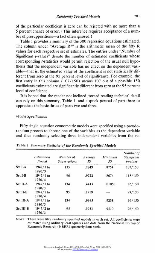
Table 1 provides a summary of the 300 regression equations estimated. The column under "Average R2" is the arithmetic mean of the fifty R values for each respective set of estimates. The entries under "Number of Significant t-values" denote the number of estimated coefficients whose corresponding t-statistics would permit rejection of the usual null hypothesis that the independent variable has no effect on the dependent variable-that is, the estimated value of the coefficient is not statistically different from zero at the 95 percent level of significance. For example, the first entry in this column (107/150) means 107 out of a possible 150 coefficients estimated are significantly different from zero at the 95 percent level of confidence.

It is hoped that the reader not inclined toward reading technical detail can rely on this summary, Table 1, and a quick perusal of part three to appreciate the basic thrust of parts two and three.

Model Specification

Fifty single-equation econometric models were specified using a pseudo- random process to choose one of the variables as the dependent variable and then randomly selecting three independent variables from the re-

Table. 1 Summary Statistics of the Randomly Specified Models

Number of Estimation Number of A verage Minimum Significant

Period Observations R2 R2 t-values

SetI-A 1947/1 to 135 .9849 .8754 107/150 1980/3

SetI-B 1947/1 to 96 .9722 .8674 118/150 1970/4

Set II-A 1947/1 to 134 .4413 .01050 85/150 1980/ 3

Set-IIB 1947/1 to 95 .2919 99/150 1970/4

SetIII-A 1947/1 to 134 .9945 .9238 99/150 1980/3

Set III-B 1947/2 to 95 .9933 .9510 96/150 1970/3

NOTE: There were fifty randomly specified models in each set. All coefficients were estimated using ordinary least squares and data from the National Bureau of Economic Research (NBER) quarterly data bank.




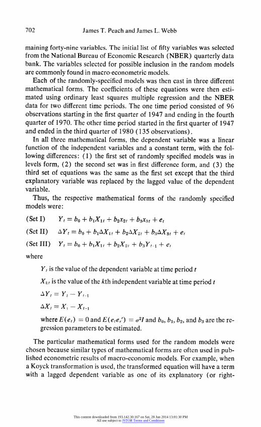
maining forty-nine variables. The initial list of fifty variables was selected from the National Bureau of Economic Research (NBER) quarterly data bank. The variables selected for possible inclusion in the random models are commonly found in macro-econometric models.

Each of the randomly-specified models was then cast in three different mathematical forms. The coefficients of these equations were then estimated using ordinary least squares multiple regression and the NBER data for two different time periods. The one time period consisted of 96 observations starting in the first quarter of 1947 and ending in the fourth quarter of 1970. The other time period started in the first quarter of 1947 and ended in the third quarter of 1980 (135 observations).

In all three mathematical forms, the dependent variable was a linear function of the independent variables and a constant term, with the following differences: (1) the first set of randomly specified models was in levels form, (2) the second set was in first difference form, and (3) the third set of equations was the same as the first set except that the third explanatory variable was replaced by the lagged value of the dependent variable.

Thus, the respective mathematical forms of the randomly specified models were:

(Set I) Yt = bo + b1Xjt + b2x2t + b3x3t + et

(Set II) AYt = bo + blAX1t + b2AX2t + b3AX3t + et

(Set III) Yt = bo + b1Xjt + b2X2t + b3Yt-l + et

where

Yt is the value of the dependent variable at time period t

Xkt is the value of the kth independent variable at time period t

Ayt yt -Yt

AX, Xt, -Xt_

where E(et) = 0 and E(eter') = a2I and bo, bl, b2, and b3 are the regression parameters to be estimated.

The particular mathematical forms used for the random models were chosen because similar types of mathematical forms are often used in published econometric results of macro-economic models. For example, when a Koyck transformation is used, the transformed equation will have a term with a lagged dependent variable as one of its explanatory (or right-




hand) variables. This would correspond to the general form of the equations in Set III. That is,

if Yt = b k XrX, -r+1 where b, X are constants r=1

and 0< X < 1, it can be transformed into

Yt=bX + XY,t,

provided s is large.

If Yt = a + b XrXf_,+, then the Koyck transformation yields

Yt (a - a a) + bkXt + XYt-1

The Type III random-model specification is thus consistent with the Koyck transformation widely used in macro-models, since in Set III b, could be interpreted as (a - Aa), b1 as bX, and b:, as A.

First differencing of variables (as in Set IL) is also a frequently en- countered transformation of a regression equation where there is serial correlation assumed to be generated by a first-order Markov process of the form

et = pet- + Vt

E(Vt) = 0 and E(Vt V1') = 0,2I andp - 1.

Thus the Gauss-Markov Theorem applies for OLSE use to estimate the first-differenced equations.

Results of Estimation

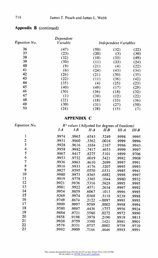
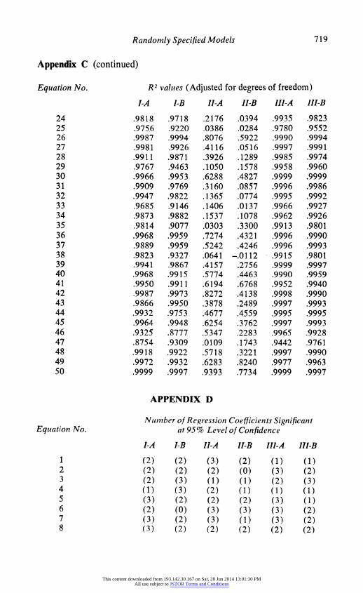
On the average, the randomly specified models have good fits to the data points. (Appendix B has the individual specifications in tabular form and Appendices C and D have individual adjusted R2 values and number of significant t-values in each individual estimation.) In levels form (I-A and I-B), thirty-two out of the fifty estimated equations had values of R2's greater than 0.99 and forty-seven had R2's above 0.95 for the longer period (I-A), and thirty-nine were greater for the shorter period (I-B). Looking at the t-statistics for the levels equation, 107 out of 150 estimated coefficients were significantly different from zero at the 95 percent level of significance for I-A estimates and 118 out of 150 were significant for the shorter period levels models (Set I-B).

For the first-differenced models regressed on the longer period (II-A),




the average R2 value for the fifty estimated equations was .4413 and six- teen of the fifty equations had R2 values above 0.60 and five were above 0.80. For the shorter period, the models in first differenced form (Set II-B) had the worst fits. The average R2 was 0.2919 and thirty-two of the fifty equations had R2 values below 0.40; twelve were below 0.05 and only three were above 0.75. Looking at the t-tests, 85 out of 150 and 61 out of 150 coefficients were statistically significant for 1I-A and II-B, respectively.

For the equations with a lagged dependent variable included on the right-hand side of the equation, R2 values were extremely high and the average R2 values were .9945 for 111-A and .9933 for III-B. In fact, forty- five out of fifty III-A equations had R2 values above 0.99 and forty of fifty R2's were greater than 0.99 for III-B.

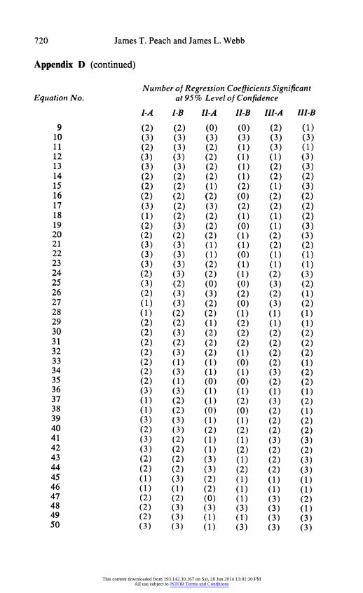
For some individual specifications the shorter time period resulted in higher R2 values than the longer period for the same included variables, and some individual estimations had higher R values in levels form (Type I) than in the form with lagged dependent variables on the right hand side (Type III). Reading across the rows of Appendix D shows no clear relationship between mathematical form (or length of time period) and number of estimated coefficients significantly different from zero at the 95 percent level of confidence. The implications for dedicated data-mining of macroeconomic time-series (increasingly facilitated by improvements in computer capabilities and software packages) should be clear.

Comparison with Models in the Literature

The examples that follow were chosen because the mathematical form and types of data were quite similar to the random models and because the results either appeared in prestigious journals or were presented by economists with established reputations in empirical econometric work with macro-models.

Model Selection Criteria

The focus of this article is on the application of econometric techniques as typically used by economic researchers in choosing among competing hypotheses in macroeconomics. Judging by what has been influential among academic economists in making these choices and what is still ac- ceptable to the leading economics journals (such as [Irvine 1981]), the traditional measures of goodness of fit (adjusted R2 and t-tests of the null hypotheses for the estimates of individual regression coefficients) have




been and continue to be the principle criteria for model selection rather than various forms of residual analysis. Perhaps one explanation for this is that software packages that include sophisticated residual analysis have only recently become widely available.

But in any event using traditional measures of statistical goodness of fit to choose among rival models (that is, models with the same dependent variables) estimated over the same data and time periods has been explicitly advocated, for example, by Dale Jorgenson and C. D. Siebert [1968], Henri Theil [1961, pp. 212-14], and Franco Modigliani and R. Sutch [1969], and is widely practiced despite the formal arguments such as those by Pheobus Dhrymes [1970] and M. H. Pesaran [1974] advanced against this practice and the demonstration by Thomas Mayer [1975] that there is a low degree of rank order correlation between size of residual variation of rival time-series models fitted to a sample period and the predictive accuracy of the models thus estimated in a post-sample period. Thus, the random results are compared with models from the literature as to adjusted R2 values and t-ratios.

Models of Type I

Lawrence R. Klein [1966] provides an example of a model like the Type I random models in mathematical form and types of data used. In this example Y is non-farm, residential construction, X1 is personal disposable income, X2 is an index of the relationship between building costs and rent, and X3 is a measure of the spread between long-term corporate bonds and short-term commercial paper. All three coefficients are significant at the 95 percent level. The R2 for the equation reported is 0.820.

Models of Type 11

A. A. Walters [19651 used a monetarist model of the same form as the randomly specified equations in Set II where his dependent variable was the change in aggregate income (that is, AYt = change in aggregate income) regressed on the changes in money supply with various lags (that is, AX1 was the change in the monetary aggregate in t -1, AX2 was the change in the money supply in t - 2, etcetera).

Walters estimated two different equations of this type for the United Kingdom using 81 annual observations. The R2 values were 0.54 and 0.46 and five of the six estimated coefficients had significant t-values compared to t-values for the first-differenced random models, slightly less than half of which were significant.




A version of the multi-equation macro-model developed at the Whar- ton School provides another example of estimated econometric equations similar to Set II (dependent and independent variables in differenced form) from a Keynesian framework [Evans 1969, pp. 305-309]. In modeling sectoral price behavior, this model sets up several equations whose dependent variables are changes in price indices for various sectors (consumer non-durables, automobiles, exports, etcetera) and regress these on independent variables-some or all of which are changes in price indices in other sectors of the economy (for example, farm products, wholesale goods, etcetera). The equation that has the exact form of the Set II equations regress the change in the price index for consumer non- durables and services on the changes in the farm price index, the wholesale price index, and the wholesale price index lagged a quarter. The R2 statistic is 0.672 and two of the three regression coefficients are significantly different from zero at the 95 percent level of confidence, while the coefficient on the other dependent variable is not statistically significant at even the 50 percent level of confidence.

Other equations estimated similar to the Set II form (but differing usually in that some of the dependent variables are in levels rather than first differences) have R2 statistics less than 0.60 (ranging from 0.439 to 0.564) except for the equation on price changes in consumer durables, which had a value of 0.682 for R2. All the remaining regression coefficients were statistically significant at the 95 percent level of confidence.

Models of Type III

A recent example of empirical research resembling equations of Type III was Owen Irvine's study of retailing inventory investment, which used macro-time-series data similar to the data used in the random models. Irvine uses NBER variables-some of which are identical to those appear- ing in the random models-and other time series sources including the Survey of Current Business and other Bureau of Economic Analysis data [Irvine 1981].

Irvine estimates several different equations with various categories of business inventory as the dependent variables included on the right-hand side of the equations in lagged form (this specification is rationalized on a partial-adjustment model rather than a Koyck-lag model).

The Irvine model differs from the random models of Type II-B in that he uses a shorter time period (March 1958 through December 1974 versus 1947/1st quarter through 1970/4th quarter), but Irvine has a larger number of observations because he uses monthly data (rather than the quar-




terly data used in the random models estimation), and in that Irvine has six variables on the right-hand-side including the lagged-dependent variable in most of his specifications (compared to three in the random models) and in that he uses an instrumental variables technique (versus ordinary least squares in random models estimation).

Irvine estimates eleven equations with R2 values ranging from .994 to .972. The average R2 for the comparable Ill-B random models was .9933 and the low value was .9510. Irvine has seven out of an estimated eleven equations containing at least one estimated coefficient failing to pass the t-test of significance at the 95 percent level of confidence. Irvine has fifty- six out of sixty-four estimated coefficients significant (88 percent) versus ninety-six out of 150 (63 percent) for the random model specifications.

The classic use of the Type III model specification is in the Koyck-lag models of the consumption function. Michael Evans presents a comparison of consumption function estimates including one specification Yt = b1Xt + bYt-1 that has the R2 value of 0.998 and both estimated coefficients significant [Evans 1969, p. 65]. Among the random model estimations, Type Ill-B is most similar to the specification. Twenty-six of the fifty equations estimated in Set Ill-B had R2 values of 0.9990 or greater.

Conclusions from Comparisons

The authors make no claim that the examples chosen from the literature are ideally representative of econometric applications, since there was no attempt at an exhaustive examination of all published econometric work comparable in form to the authors' randomly specified models and con- sequent estimation of "mean R2's." Rather the authors believe that the examples presented are illustrative of the type of economic work taken seriously in the profession. The essential point is simply this: a large pro- portion of models generated randomly are indistinguishable from models based on accepted theoretical frameworks and estimated by respected investigators if the usual tests of goodness of fit and statistical significance are the only criteria used.

Lessons from Methodology

For hard sciences, the misguided methodological beliefs of individual scientists may have little practical effect on the growth of knowledge in that particular discipline. However, the random-model results suggest that as a practical matter the intellectually honest but methodologically naive economic researcher may find that econometric testing is highly incon-




clusive. Therefore, it is worthwhile to examine the best methodological perspectives for insights on choices between competing hypotheses. Un- fortunately, economists advocate and practice a number of discredited methodological positions that have the effect of reducing the impact of empirical evidence on theoretical beliefs. Even though the most refined version of the logical-positivist philosophy of science has been found inadequate, economists continue to espouse discredited early versions of this view.

Frederick Suppe [1977] provides an extremely useful summary of the current status of what economists would call methodological issues among the community of philosophers of science, especially in his introductory essay "The Search for Philosophic Understanding of Scientific Theories" and in his "Afterword" [1977]. The rise and fall of the positivistic philosophy of science is treated on pages 3-118. Nevertheless Paul Samuelson [1964] advocates "operationalism," a long-discredited version of early positivistic philosophy of science.2

To the extent that the positivistic emphasis on formalism and inter- theoretic reduction has influenced economics, attention is diverted from empirical testing. Economic methodologies based on confirmationism severely reduce the impact of empirical facts on theory choice since there are very few theories that cannot find some empirical support. A confirmationist methodology also encourages scientific investigators to examine empirical evidence selectively and to discount new evidence once a theory is considered sufficiently confirmed-that is, old facts have more weight than new facts in evaluating theories with a confirmationist methodology. Aside from the practical reasons for rejecting a methodology based on confirmation (or "verification" or "validation") of hypotheses, it is simply illogical. As Karl Popper [1959, p. 374n] points out, there can be two contradictory theories that both predict the same observable event. That the predicted event is in fact observed merely means neither theory has been refuted; it is absurd to say the mutually exclusive theories have both been verified. And it is always possible to devise an alternative theory that would predict the observed event.

However, the most anti-empirical methodology of all is the view that theories are simply convenient devices (or instruments) for generating predictions and nothing more.3 Thus construed, theoretical instruments can never be falsified-they are useful or not in the particular context. As used by economists in its "as-if" or "irrelevance-of-assumptions" version, this view has the effect of reducing the permissible range of empirical tests -that is, empirical tests of "assumptions" are ruled illegitimate even if




feasible [Friedman 1953; Boland 1980]. For these and other reasons this position has been denounced by sophisticated positivist philosophers of science and by refutationist critics of positivist philosophy of science [Lakatos 1970; Caldwell 1980]. For example, after surveying methodological positions, Mark Blaug [1980, p. 128] concludes: "The prevailing methodological mood is not only highly protective of received economic theory, it is also ultrapermissive within the limits of the 'rules of the game.' . . . Modern economists frequently preach falsificationism ... but they rarely practice it: their working philosophy of science is aptly de- scribed as 'innocuous falsificationism.' "

Imre Lakatos's Methodology of Scientific Research Programmes (MSRP) escapes the criticisms to which these discredited views are subject while permitting a progressive and rationally-based methodology that is not contrary to actual scientific practice (at least scientists are not called upon to abandon a successful research agenda on the basis of one or a few instances of empirical counterevidence) [Lakatos 1970, pp. 132-38]. A description of the structure of scientific theories consistent with Lakatos's MSRP (but couched in terminology used to describe logical positivist views) would contain the following elements: (1) 1, a set of theoretical postulates perhaps (but not necessarily) containing unobservable theoretical terms; (2) C, an interpretative system (consisting of theories of observation and measurement, rules for the empirical applicability of the theory, auxiliary hypotheses, etcetera) necessary to connect theoretical postulates to empirical events; and (3) E, a set of empirical events hy- pothesized by a conjunction of T and C.

Empirical testing would involve generating some particular observable hypothesis, say E1, from the conjunction of the body of theory and its interpretative system and subjecting this hypothesis to an empirical test where the observation of Et is possible.4 Indeed, the scientific investigator would attempt to devise tests that maximize the probability that -E1 could be observed if the aggressive methodological prescriptions of Pop- per [1959; 1962] are followed.

If T and T' are competing bodies of theory, T' would be preferable to T if T' (in conjunction with its interpretative system) could predict all the events E predicted by T plus additional events not predicted by T, say E', and if some of this excess empirical content (of T' over T) had empirical corroboration (that is, some of the predictions in E' had been empirically tested and not refuted).

This account should not be construed to mean that all the elements in a body of theory can be formalized. In fact, if the theory in question is




part of a progressive research agenda (that is, new hypotheses are being generated and tested without all being refuted), the theory will contain non-formalizable elements in addition to the formalizable theoretical postulates [Popper 1962, pp. 74n]. This is a central lesson of the weltan- schaungen theorists such as N. R. Hanson, Thomas Kuhn, and Stephen Toulmin, and is one reason the Lakatosian "hard-core" is distinguished from the "protective belt" [Lakatos 1970, pp. 132-37].5

Moreover, the interpretative system connecting theoretical postulates to empirical events must employ a language richer and more versatile than the artificial languages currently amenable to rigorous logical analysis. That is, theoretical growth and empirical testability necessarily involve some logical and linguistic looseness. By ignoring these subjective elements economists are able to emphasize the formal elements of hypothesis testing and to assume that the linkage of theoretical constructs to their empirical counterparts is unproblematical. This formalism creates the illusion of great rigor while in fact making the connection between theoretical concepts and observed events longer and looser and much more subjective.

Implications for Econometric Testing of Economic Hypotheses

The central lesson from the discussion of methodology is that any empirical test of a hypothesis is inconclusive and some conventionalist tactics are justifiable even with a sophisticated refutationist methodology. These conventionalist tactics (altering observational theories, appeals to unful- filled ceteris paribus conditions, questioning quality of data after the fact, etcetera) can include switches in econometric technique, changes in assumptions about probability distributions, and respecification of regression models.

In the notation use above, changing estimation techniques, revising assumptions about distributions, or transforming observed values of variables amounts to substituting a new interpretative system C* for the pre- vious interpretative system C, and there is no necessary reason at all to expect this change to bring the choice between competing bodies of theory, T and T', closer to a resolution. In fact, casual empiricism might suggest the opposite is true in economics-that cleverness in reformulation of C is most often used to reconcile accepted theories with anomalous data. Resolving the choice between competing bodies of theory is not simply a matter of choosing the technically correct statistical method.

A tighter statistical fit does not necessarily bring the theory choice issue




closer to resolution-for example, revising the combinations of statistical technique, regression model, and data (and data transformation) to achieve closer correlation between individual incomes and educational levels does not bring one closer to deciding whether the human capital theory is superior to Marxian explanations of the correlation between education (viewed by Marxians as a measure of class status) and income.

That in principle any given empirical test is inconclusive might not matter if in practice the facts were so recalcitrant as to weed out unsound theories. But the nature of economic phenomena-especially macroeconomic phenomena-is such that it is in practice quite common to achieve a close statistical fit between almost any combination of macro-variables as the first section of this article illustrates. At least this should demonstrate the consequences of permitting claims of "verification" (or "validation" or "confirmation") to be made on the basis of achieving high levels of correlation. If the economics profession accepts the irrelevance-of- assumptions thesis (and other discredited methodological views) in addition to confirmationism, the power of empirical evidence to change theoretical beliefs is diluted almost to nothing.

Since in principle empirical testing of macroeconomic hypotheses is inconclusive and in practice the degre of inconclusiveness is likely to be large, other theory evaluation criteria supplement empirical testing. Often the supplementary criteria are implicit and rely on appeals to authority, "oral traditions," etcetera, and are ad hoc and highly subjective. Consid- ering supplementary theory evaluation explicitly, emphasizing criteria such as simplicity, amenability to mathematical manipulation, and gen- erality contributes to formalism and diminishes the role of empirical evidence in theory choice.

Moreover, the intuitive notion of simplicity, which usually involves smooth curves, fewer variables, less complex mathematical forms, etcetera, has not been formalized in a way that does not permit counterintuitive examples [Hess 1967, pp. 445-48; Sober 1975]. "Simplicity" is a theory- evaluation criterion characteristic of methodologies emphasizing conven- tionalism at the expense of empirical testing [Caldwell 1980, p. 367]. Aside from this, the criterion of "simplicity" can be expected to produce specification errors as relevant variables are omitted or as simpler mathematical forms are substituted for the true equation [Johnston 1972, pp. 168-69; Kmenta 1971, pp. 391-405].

On the other hand, requiring that economic theory be coherent with other bodies of accepted scientific knowledge provides additional points of contact with reality as does emphasizing the explanatory role of eco-




nomic theories, since explanations ordinarily involve generalizations be- lieved to be true (for example, unrefuted scientific theories from other disciplines and empirical knowledge).

Conclusions

The intent of the authors is constructive. This article is meant to con- tribute to making economics a more genuinely progressive empirical science. The argument proceeded as follows: (1) The random model experiment and comparisons with the literature indicate (at least for macroeconomic models and conventional goodness of fit tests) that naive application of technique is inadequate and inconclusive for choosing among competing hypotheses; (2) thus the authors examined methodological issues in order to reduce this inconclusiveness.

(3) Some methodological views advocated by economists are illogical and antiempirical in their effect and add to the inconclusiveness. The irrelevance-of-assumptions thesis, the worst of these views, is downright antiscientific. (4) However, the discussion of methodology reveals that even with a defensible methodology (such as that of Lakatos), conventionalist tactics can be justified (that is, reformulation of the interpretative system can be used to "save" a theory from anomalous facts). But this same discussion should alert readers that there is no particular reason to suppose that reformulation of the interpretative system will reduce the inconclusiveness of econometric testing of competing hypotheses. More bluntly stated, the problem of inconclusiveness is not simply a technical problem awaiting solution as more sophisticated econometric technique is developed.

(5) What is needed is for empirical investigators to formulate hypotheses in such a way that competing theories can be discriminated among on the basis of the econometric results. (This is not done by human capital theorists who regress income on education-the education-productivity and productivity-income links are the crucial foci for generating such hypotheses.)

(6) Theory should make empirical contact in every way possible. Every testable assumption should be tested. The relationships between proxy variables and their counterparts should be examined. Explanatory power should be considered a virtue for theory but this is precluded by the doctrine that theories are merely predictive instruments and nothing more (that is, the irrelevance-of-assumptions doctrine with its most charitable of interpretations).




Notes

1. This symposium on December 28, 1981, was chaired by Jan Kmenta and included Vernon Smith, Zvi Griliches, Karl Brunner, Lawrence Klein, R. J. Gordon, James Heckman, and Jacob Frenkel as participants.

2. Operationalism is a form of reductionism, the doctrine propounded by early positivist philosophers of science that to be meaningful each theoretic term had to be separately expressible in terms of an empirically observable counterpart. There are numerous difficulties with this doctrine since, for example, much of accepted theory in physics would not be "meaningful" by this doctrine. More to the point, Samuelson's reductionism has the same practical effect as M. Friedman's methodological instrumentalism-both tend to immunize accepted theory from empirical refutation. (See [Suppe 1977, pp. 20-22, Wong 1973] and footnote 3 in this article.)

3. Among philosophers of science the doctrine that scientific theories should serve as instruments for the generation of predictions and nothing more is called "instrumentalism" following Popper's use of the term in "Three Views Concerning Human Knowledge" (in [Popper 1962]). However, since institutionalists have used the term "instrumentalism" with a different meaning, we have avoided the word altogether in the text. It would be worthwhile to discuss the distinctions and connections between "instrumentalism" in the sense of Popper and "instrumentalism" as the term is used by John Dewey, Clarence Ayres, and other institutionalists but it would require a full-length article to do it justice.

4. The symbol -E1 means the negation of E1. 5. Lakatos's "hard core" is much the same as Kuhn's "paradigm" (in the

sense of disciplinary matrix). This is that portion of the body of theory and accompanying ontological beliefs that distinctively characterize a theory and to which scientists accepting the theory hold most tenaciously. The "protective belt" more or less corresponds to those parts of the interpretive system that scientists are quite willing to alter in order to reconcile anomalous facts to accepted theory, thus permitting accepted theory to be maintained in the face of what previously were anomalous facts. An important implication of Lakatos's methodology (which is superior to methodological positions advocated by most economists) is that theories always contain nonformalizable elements (which some might choose to call "metaphysical"). An emphasis on the logical manipulation of those elements of theory that are formalizable does not make non-formalized elements of theory less crucial nor is it a substitute for genuine empiricism.

References

Ames, Edward, and Stanley Reiter. 1961. "Distributions of Correlation Co- efficients in Economic Time Series." Journal of the American Statistical As- sociation 56 (September): 637-56.

Blaug, Mark. 1980. The Methodology of Economics: Or How Economists Explain. Cambridge: Cambridge University Press.




Boland, Lawrence. 1980. "A Critique of Friedman's Critics." Journal of Eco- nomic Literature 47 (October): 366-74.

Caldwell, Bruce J. 1980. "A Critique of Friedman's Methodological Instru- mentalism." Southern Economic Journal 47 (October): 366-74.

Cooley, Thomas F., and Stephen F. LeRoy. "Identification and Estimation of Money Demand." American Economic Review 71 (December): 825-44.

Dhrymes, Pheobus. 1970. "On the Game of Maximizing R2." Australian Eco- nomic Papers 9 (December): 177-85.

Evans, Michael. 1969. Macroeconomic Activity Theory, Forecasting and Con- trol: An Econometric Approach. New York: Harper & Row.

Friedman, Milton. 1953. "The Methodology of Positive Economics," in his Essays in Positivist Economics. Chicago: University of Chicago Press.

Frisch, Ragnar. 1981. "From Utopian Theory to Practical Applications: The Case of Econometrics." American Economic Review 71 (December): 1-7.

Hesse, Mary. "Simplicity." Encyclopedia of Philosophy. Vol. 7. New York: Macmillan, The Free Press.

Irvine, Owen. 1981. "Retail Inventory Investment and the Cost of Capital." American Economic Review 71 (September): 633-48.

Johnston, John. 1972. Econometric Methods. 2d ed. New York: McGraw- Hill.

Jorgenson, Dale, and C. D. Siebert. (1968). "Theories of Corporate Invest- ment Behavior." American Economic Review 58 (September): 681-712.

Klein, Lawrence R. 1966. The Keynesian Revolution, 2d ed. New York: Mac- millan.

Kmenta, Jan. 1971. Elements of Econometrics. New York: Macmillan. Kuhn, Thomas S. 1970. The Structure of Scientific Revolutions, 2d ed. enl.

Chicago: University of Chicago Press. Lakatos, Imre. 1970. "Falsification and the Methodology of Scientific Re-

search Programmes," in Criticism and the Growth of Knowledge, ed. by Imre Lakatos and Alan Musgrave. Cambridge: Cambridge University Press.

Leamer, Edward. 1978. Specification Searches: Ad Hoc Inferences with Non- Experimental Data. New York: Wiley.

Mayer, Thomas. 1975. "Selecting Economic Hypotheses by Goodness of Fit." Economic Journal 85 (December): 877-83.

_ 1980. "Economics as a Hard Science: Realistic Goal or Wishful Thinking." Economics Inquiry 18 (April): 165-78.

Modigliani, Franco, and R. Sutch. 1969. "The Term Structure of Interest Rates: A Reexamination of the Evidence." Journal of Money, Credit, and Banking 1 (February): I 1 2-20.

Pesaran, M. H. 1974. "On the General Problem of Model Selection." Review of Economic Studies 61 (April): 153-71.

Pierce, David. 1977. "Relationships-and the Lack Thereof-Between Eco- nomic Time Series, with Special Reference to Money and Interest Rates." Journal of the American Statistical Association 72 (March): 11-22.

Popper, Karl R. 1959. The Logic of Scientific Discovery. New York: Basic Books.

1962. Conjectures and Ref utations. New York: Basic Books. Ramsey, James R., and Jan Kmenta. 1980. "Problems and Issues in Evaluating




Econometric Models," in Evaluation of Econometric Models, edited by James R. Ramsey and Jan Kmenta. New York: Academic Press.

Samuelson, Paul A. 1964. "Theory and Realism: A Reply." American Eco- nomic Review 54 (September): 736-39.

Sober, Eliott. 1975. Simplicity. Oxford: Oxford University Press. Suppe, Frederick. 1977. The Structure of Scientific Theories, 2d ed. Urbana:

University of Illinois Press. Theil, Henri. 1961. Economic Forecasts and Policy. Amsterdam: North Hol-

land. Walters, A. A. 1965. "Professor Friedman on the Demand For Money." Jour-

nal of Political Economy 73 (October): 545-5 1. Wong, Stanley. 1973. "The F-Twist and the Methodology of Paul Samuelson."

American Economic Review 63 (June): 312-25.

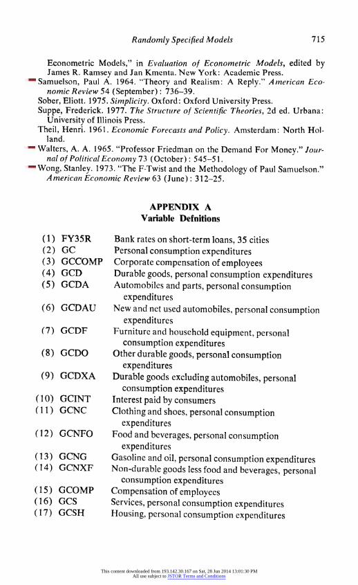
APPENDIX A Variable Defnitions

(1) FY35R Bank rates on short-term loans, 35 cities (2) GC Personal consumption expenditures (3) GCCOMP Corporate compensation of employees (4) GCD Durable goods, personal consumption expenditures (5) GCDA Automobiles and parts, personal consumption

expenditures (6) GCDAU New and net used automobiles, personal consumption

expenditures (7) GCDF Furniture and household equipment, personal

consumption expenditures (8) GCDO Other durable goods, personal consumption

expenditures (9) GCDXA Durable goods excluding automobiles, personal

consumption expenditures (10) GCINT Interest paid by consumers (11) GCNC Clothing and shoes, personal consumption

expenditures (12) GCNFO Food and beverages, personal consumption

expenditures (13) GCNG Gasoline and oil, personal consumption expenditures (14) GCNXF Non-durable goods less food and beverages, personal

consumption expenditures (15) GCOMP Compensation of employees (16) GCS Services, personal consumption expenditures (17) GCSH Housing, personal consumption expenditures




(18) GCSHO Household operation, personal consumption expenditures

(19) GCSIN Contributions for social insurance (20) GCSO Other services, personal consumption expenditures (21) GCST Transportation, personal consumption expenditures (22) GCSUPP Corporate supplements to wages and salaries (23) GCTTS Indirect business taxes plus transfer payments less

subsidies (24) GCW Corporate wages and salaries (25) GDC Implicit price deflator, personal consumption

expenditures (26) GDNNP Implicit price deflator, net national product (27) GEX Export of goods and services (28) GGAID Federal expenditures, grants in aid to state and local

government (29) GGE Government purchases of goods and services (30) GGFE Federal government purchases of goods and services (31) GGFEN Federal government purchases for national defense (32) GGFEO Federal government purchases for other than

national defense (33) GGFPT Personal tax and non-tax receipts, federal government (34) GGSE State and local government purchases of goods and

services (35) GGSPT Personal tax and non-tax receipts, state and local

government (36) GIF Fixed private domestic investment (37) GIM Imports of goods and services (38) GIN Non-residential private domestic investment (39) GIR Residential structures, private domestic investment (40) GNP Gross national product (41) GNS Final sales, total (42) GOD Durable goods output (43) GODA Gross auto output (44) GPOP Population, including armed forces, mid-quarter (45) GPRENT Rental income of persons (46) GPROJ Proprietors' income (47) GY National income (48) GYD Disposable personal income (49) LBPUR Compensation per hours, non-farm business sector (50) LCPM Compensation per man-hour in manufacturing




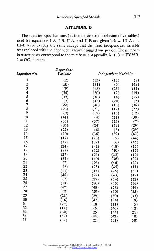
APPENDIX B

The equation specifications (as to inclusion and exclusion of variables) used for equations I-A, I-B, 11-A, and II-B are given below. Ill-A and III-B were exactly the same except that the third independent variable was replaced with the dependent variable lagged one period. The numbers in parentheses correspond to the numbers in Appendix A: (1) = FY35R, 2 = GC, etcetera.

Dependent Equation No. Variable Independent Variables

1 (2) (13) (12) (8) 2 (50) (31) (5) (45) 3 (9) (18) (25) (12) 4 (34) (20) (2) (19) 5 (39) (36) (8) (15) 6 (7) (43) (20) (2) 7 (22) (46) (13) (36) 8 (23) (21) (12) (22) 9 (9) (17) (18) (12)

10 (41) (4) (21) (38) 11 (33) (37) (23) (7) 12 (35) (24) (49) (29) 13 (22) (6) (8) (29) 14 (10) (36) (29) (42) 15 (17) (23) (5) (44) 16 (35) (39) (6) (45) 17 (24) (42) (18) (15) 18 (37) (12) (40) (15) 19 (27) (26) (25) (10) 20 (32) (40) (36) (29) 21 (7) (26) (46) (20) 22 (6) (25) (45) (11) 23 (14) (13) (25) (26) 24 (46) (22) (43) (42) 25 (7) (27) (14) (22) 26 (18) (20) (15) (16) 27 (47) (48) (28) (44) 28 (8) (29) (50) (35) 29 (28) (29) (50) (33) 30 (16) (42) (24) (9) 31 (29) (18) (11) (5) 32 (14) (6) (46) (12) 33 (30) (25) (44) (21) 34 (37) (44) (42) (18) 35 (32) (21) (31) (38)




Appendix B (continued)

Dependent Equation No. Variable Independent Variables

36 (47) (50) (32) (22) 37 (23) (20) (3) (30) 38 (32) (10) (33) (49) 39 (50) (11) (33) (24) 40 (9) (21) (4) (22) 41 (6) (24) (43) (34) 42 (26) (21) (50) (35) 43 (22) (11) (36) (42) 44 (35) (4) (25) (23) 45 (40) (49) (17) (29) 46 (30) (36) (18) (32) 47 (1) (38) (12) (22) 48 (22) (18) (33) (36) 49 (30) (31) (27) (50) 50 (24) (28) (15) (7)

APPENDIX C

Equation No. R2 values (Adjusted for degrees of freedom) I-A I-B II-A Il-B 111-A Ill-B

1 .9974 .9965 .6543 .5249 .9998 .9995 2 .9931 .9860 .3362 .0016 .9999 .9996 3 .9928 .9616 .1684 .2167 .9986 .9943 4 .9958 .9982 .7417 .4653 .9999 .9997 5 .9867 .9417 .8275 .5101 .9899 .9706 6 .9953 .9732 .6019 .5421 .9982 .9908 7 .9936 .9863 .4610 .2699 .9997 .9991 8 .9916 .9933 .4176 .3207 .9995 .9993 9 .9927 .9595 .0550 .0331 .9985 .9941

10 .9980 .9973 .8365 .6882 .9998 .9997 11 .9919 .9778 .3365 .1044 .9980 .9932 12 .9921 .9836 .5316 .5628 .9995 .9995 13 .9981 .9922 .4571 .2634 .9997 .9992 14 .9954 .9859 .6067 .1013 .9996 .9995 15 .9269 .9974 .0368 .3118 .9238 .9998 16 .9749 .8674 .2122 -.0097 .9995 .9995 17 .9999 .9997 .9589 .8002 .9998 .9994 18 .9580 .9887 .4436 .1757 .9956 .9924 19 .9684 .9721 .5560 .0272 .9972 .9890 20 .9858 .9198 .3978 .2190 .9919 .9813 21 .9938 .9759 .3380 .1421 .9981 .9901 22 .9578 .9331 .0737 .0002 .9759 .9510 23 .9982 .9909 .7166 .4646 .9993 .9991




Appendix C (continued)

Equation No. R2 values (Adjusted for degrees of freedom)

I-A i-B II-A Il-B III-A Ill-B

24 .9818 .9718 .2176 .0394 .9935 .9823 25 .9756 .9220 .0386 .0284 .9780 .9552 26 .9987 .9994 .8076 .5922 .9990 .9994 27 .9981 .9926 .4116 .0516 .9997 .9991 28 .9911 .9871 .3926 .1289 .9985 .9974 29 .9767 .9463 .1050 .1578 .9958 .9960 30 .9966 .9953 .6288 .4827 .9999 .9999 31 .9909 .9769 .3160 .0857 .9996 .9986 32 .9947 .9822 .1365 .0774 .9995 .9992 33 .9685 .9146 .1406 .0137 .9966 .9927 34 .9873 .9882 .1537 .1078 .9962 .9926 35 .9814 .9077 .0303 .3300 .9913 .9801 36 .9968 .9959 .7274 .4321 .9996 .9990 37 .9889 .9959 .5242 .4246 .9996 .9993 38 .9823 .9327 .0641 -.0112 .9915 .9801 39 .9941 .9867 .4157 .2756 .9999 .9997 40 .9968 .9915 .5774 .4463 .9990 .9959 41 .9950 .9911 .6194 .6768 .9952 .9940 42 .9987 .9973 .8272 .4138 .9998 .9990 43 .9866 .9950 .3878 .2489 .9997 .9993 44 .9932 .9753 .4677 .4559 .9995 .9995 45 .9964 .9948 .6254 .3762 .9997 .9993 46 .9325 .8777 .5347 .2283 .9965 .9928 47 .8754 .9309 .0109 .1743 .9442 .9761 48 .9918 .9922 .5718 .3221 .9997 .9990 49 .9972 .9932 .6283 .8240 .9977 .9963 50 .9999 .9997 .9393 .7734 .9999 .9997

APPENDIX D

Number of Regression Coefficients Significant Equation No. at 95% Level of Confidence

I-A I-B Il-A il-B Ill-A Ill-B

1 (2) (2) (3) (2) (1) (1) 2 (2) (2) (2) (0) (3) (2) 3 (2) (3) (1) (1) (2) (3) 4 (1) (3) (2) (1) (1) (1) 5 (3) (2) (2) (2) (3) (1) 6 (2) (0) (3) (3) (3) (2) 7 (3) (2) (3) (1) (3) (2) 8 (3) (2) (2) (2) (2) (2)




Appendix D (continued)

Number of Regression Coefficients Significant Equation No. at 95 % Level of Confidence

1-A 1-B 11-A 11-B 111-A 111-B

9 (2) (2) (0) (0) (2) (1) 10 (3) (3) (3) (3) (3) (3) 12 (3) (3) (2) (1) (1) (3) 13 (3) (3) (2) (1) (2) (3) 14 (2) (2) (2) (1) (2) (2) 15 (2) (2) (1) (2) (1) (3) 16 (2) (2) (2) (0) (2) (2) 17 (3) (2) (3) (2) (2) (2) 18 (1) (2) (2) (1) (1) (2) 19 (2) (3) (2) (0) (1) (3) 20 (2) (2) (2) (1) (2) (3) 21 (3) (3) (1) (1) (2) (2) 22 (3) (3) (1) (0) (1) (1) 23 (3) (3) (2) (1) (1) (1) 24 (2) (3) (2) (1) (2) (3) 25 (3) (2) (0) (0) (3) (2) 26 (2) (3) (3) (2) (2) (1) 27 (1) (3) (2) (0) (3) (2) 28 (1) (2) (2) (1) (1) (1) 29 (2) (2) (1) (2) (1) (1) 30 (2) (3) (2) (2) (2) (2) 31 (2) (2) (2) (2) (2) (2) 32 (2) (3) (2) (1) (2) (2) 33 (2) (1) (1) (0) (2) (1) 34 (2) (3) (1) (1) (3) (2) 35 (2) (1) (0) (0) (2) (2)

37 (1) (2) (1) (2) (3) (2) 38 (1) (2) (0) (0) (2) (1) 39 (3) (3) (1) (1) (2) (2) 40 (2) (3) (2) (2) (2), (2) 41 (3) (2) (1) (1) (3) (3) 42 (3) (2) (1) (2) (2) (2) 43 (2) (2) (3) (1) (2) (3) 44 (2) (2) (3) (2) (2) (3) 45 (1) (3) (2) (1) (1) (1) 46 (1) (1) (2) (1) (1) (1) 47 (2) (2) (0) (1) (3) (2) 48 (2) (3) (3) (3) (3) (1) 49 (2) (3) (1) (1) (3) (3) 50 (3) (3) (1) (3) (3) (3)



Documents

Randomly Specified Macroeconomic Models: Some Implications for Model Selection