Embed Size (px)
Citation preview
Acta Numerica (2017) pp 95ndash135 ccopy Cambridge University Press 2017
doi101017S0962492917000058 Printed in the United Kingdom
Randomized algorithmsin numerical linear algebra
Ravindran KannanMicrosoft Research Labs Bangalore
Karnataka 560001 India
E-mail kannanmicrosoftcom
Santosh VempalaGeorgia Institute of Technology
North Avenue NW Atlanta GA 30332 USA
E-mail vempalagatechedu
This survey provides an introduction to the use of randomization in the designof fast algorithms for numerical linear algebra These algorithms typicallyexamine only a subset of the input to solve basic problems approximatelyincluding matrix multiplication regression and low-rank approximation Thesurvey describes the key ideas and gives complete proofs of the main resultsin the field A central unifying idea is sampling the columns (or rows) of amatrix according to their squared lengths
CONTENTS
1 Introduction 962 Basic algorithms 993 Tensor approximation via length-squared
sampling 1114 Spectral norm error for matrices 1185 Preconditioned length-squared sampling 1226 Subspace embeddings and applications 1257 Conclusion 131References 132
at httpswwwcambridgeorgcoreterms httpsdoiorg101017S0962492917000058Downloaded from httpswwwcambridgeorgcore IP address 10721314018 on 21 May 2017 at 023014 subject to the Cambridge Core terms of use available
96 R Kannan and S Vempala
1 Introduction
Algorithms for matrix multiplication low-rank approximations singularvalue decomposition dimensionality reduction and other compressed rep-resentations of matrices linear regression etc are widely used For moderndata sets these computations take too much time and space to perform onthe entire input matrix Instead one can pick a random subset of columns(or rows) of the input matrix If s (for sample size) is the number of columnswe are willing to work with we execute s statistically independent identicaltrials each selecting a column of the matrix Sampling uniformly at ran-dom (uar) is not always good for example when only a few columns aresignificant
Using sampling probabilities proportional to squared lengths of columns(henceforth called lsquolength-squared samplingrsquo) leads to many provable errorbounds If the input matrix A has n columns we define1
pj =|A( j)|2
A2F for j = 1 2 n
and in each trial pick a random X isin 1 2 n with Pr(X = j) = pj We will prove error bounds of the form εA2F provided s grows as a
function of 1ε (s is independent of the size of the matrix) for all matricesSo the guarantees are worst-case bounds rather than average-case boundsThey are most useful when A22A2F is not too small as is indeed thecase for the important topic of principal component analysis (PCA) Thealgorithms are randomized (ie they use a random number generator) andhence errors are random variables We bound the expectations or tail prob-abilities of the errors In this paper we strike a compromise between read-ability and comprehensive coverage by presenting full proofs of conceptuallycentral theorems and stating stronger results without proofs
11 Overview of the paper
The first problem we consider is computing the matrix product AAT Givenas input an mtimesn matrix A we select a (random) subset of s columns of A(in s independent identical trials) We then scale the selected columns andform an mtimes s matrix C We wish to satisfy two conditions (i) (each entryof) CCT is an unbiased estimator of (the corresponding entry of) AAT and(ii) the sum of the variances of all entries of CCT (which we refer to as
1 All matrices in this paper have real entries We use the usual norms for matrices theFrobenius norm ( middotF ) and the spectral norm ( middot2) We also use standard MATLABcolon notation ie A( j) is the jth column of A see Golub and Van Loan (1996Section 118)
at httpswwwcambridgeorgcoreterms httpsdoiorg101017S0962492917000058Downloaded from httpswwwcambridgeorgcore IP address 10721314018 on 21 May 2017 at 023014 subject to the Cambridge Core terms of use available
Randomized algorithms in numerical linear algebra 97
A
ntimesm
asymp
samplecolumns
ntimes s
multi-plier
stimes r
sample rows
r timesm
Figure 11 Approximating A by a sample of s columns and r rows
the lsquovariancersquo) is at most ε2A4F Formally
E(CCT ) = AAT E(AAT minus CCT 2F ) le ε2A4F (11)
Note that (11) implies E(AAT minusCCT F ) le εA2F by Jensenrsquos inequalityThe starting point of sampling-based matrix algorithms was the discovery
of length-squared sampling by Frieze Kannan and Vempala (1998 2004)motivated by low-rank approximation We start with two properties oflength-squared sampling which will be proved in Theorem 21
bull Length-squared sampling minimizes variance among all unbiased es-timators
bull A sample of size s = 1ε2 suffices to ensure (11) In particular s isindependent of m and n
Length-squared sampling achieves similar error bounds for general matrixmultiplication matrix sketches low-rank approximation etc The mainresult in matrix sketching is as follows For any mtimesn input matrix A forman m times s sub-matrix C of the columns of A and an r times n sub-matrix Rof the rows of A both picked using length-squared sampling We can thencompute an stimes r matrix U so that
E(Aminus CUR22) le εA2Fprovided r ge cε2 s ge cε3 This is proved in Theorem 25 A schematicdiagram of C U and R is shown in Figure 11
Section 23 shows a result based purely on matrix perturbation theory(no probabilities involved) which in words states If C and A are any twomatrices with CCT asymp AAT (CA may be of different dimensions) then therestriction of A to the space spanned by the top k singular vectors of C is agood approximation to A Used in conjunction with (11) this reduces theproblem of low-rank approximation of A to computing the singular valuedecomposition (SVD) of a submatrix C
In Section 3 we apply length-squared sampling to tensors (higher-dim-ensional arrays) to obtain good low-rank tensor approximation Unlikematrices finding the best low-rank approximation for tensors is NP-hard
at httpswwwcambridgeorgcoreterms httpsdoiorg101017S0962492917000058Downloaded from httpswwwcambridgeorgcore IP address 10721314018 on 21 May 2017 at 023014 subject to the Cambridge Core terms of use available
98 R Kannan and S Vempala
Low-rank tensor approximation has several applications and we show thatthere is a natural class of tensors (which includes dense hypergraphs andgeneralizations of metrics) for which after scaling A2 = Ω(AF ) Low-rank approximation based on length-squared sampling yields good results
In Sections 4 5 and 6 we turn to more refined error bounds for matricesCan we improve the right-hand side of (11) if we want to bound only thespectral norm instead of the Frobenius norm Using deep results fromfunctional analysis Rudelson and Vershynin (2007) showed that if we uselength-squared sampling
CCT minusAAT 2 le εA2AF holds with high probability
provided s ge c ln(1ε)
ε2 (12)
While the change from Frobenius to spectral norm was first considered forits mathematical appeal it is also suitable for the HoeffdingndashChernoff-typeinequality for matrix-valued random variables proved by Ahlswede andWinter (2002) We present this theorem and proof (Theorem 41) sinceit is of independent interest In Section 4 we prove the result of Rudelsonand Vershynin
A central question in probability is to determine how many iid samplesfrom a probability distribution suffice to make the empirical estimate of thevariance close to the true variance in every direction Mathematically thereis an n timesm matrix A (with m gt n m possibly infinite) such that AAT isthe covariance matrix and for any unit vector x isin Rn the variance of thedistribution in direction x is xTAATx = |xTA|2 The problem is to find a(small) sample of s columns of A to form an n times s matrix C so that thevariance is (approximately) preserved to relative error ε in every directionx That is we wish to satisfy for all x
xTC2 isin[(1minus ε)xTA2 (1 + ε)xTA2
] denoted xTC2 sim=ε xTA2
(13)It is important that (13) holds simultaneously for all x It turns out thatin general if we sample columns of A with probability proportional to thesquared length not of its own columns but of the columns of A+A whereA+ is the pseudo-inverse of A then (13) follows from (12) We call thislsquopreconditionedrsquo length-squared sampling (since multiplying A by A+ canbe thought of as preconditioning)
There is another seemingly unrelated context where exactly the samequestion (13) arises namely graph sparsification considered by Spielmanand Srivastava (2011) Here A is the nodendashedge signed incidence matrix of agraph and the goal is to find a subset of edges satisfying (13) Spielman andSrivastava (2011) showed in this case that the squared length of the columns
at httpswwwcambridgeorgcoreterms httpsdoiorg101017S0962492917000058Downloaded from httpswwwcambridgeorgcore IP address 10721314018 on 21 May 2017 at 023014 subject to the Cambridge Core terms of use available
Randomized algorithms in numerical linear algebra 99
of A+A are proportional to the (weighted) electrical resistances and can alsobe computed in linear time (in the number of edges of the graph)
In theoretical computer science preconditioned length-squared sampling(also called leverage score sampling) arose from a different motivation Canthe additive error guarantee (11) be improved to a relative error guaranteeperhaps with more sophisticated sampling methods Several answers havebeen given to this question The first is simply to iterate length-squaredsampling on the residual matrix in the space orthogonal to the span ofthe sample chosen so far (Deshpande Rademacher Vempala and Wang2006) Another is to use preconditioned length-squared sampling where thepreconditioning effectively makes the sampling probabilities proportional tothe leverage scores (Drineas Mahoney and Muthukrishnan 2008) A thirdis volume sampling which picks a subset of k columns with probabilitiesproportional to the square of the volume of the k-simplex they span togetherwith the origin (Deshpande and Vempala 2006 Deshpande and Rademacher2010 Anari Gharan and Rezaei 2016) We discuss preconditioned length-squared sampling in Section 5
In Section 6 we consider an approach pioneered by Clarkson and Woodruff(2009 2013) for obtaining similar relative-error approximations but in inputsparsity time ie time that is asymptotically linear in the number of non-zeros of the input matrix This is possible via a method known as subspaceembedding which can be performed in linear time using the sparsity of thematrix We first discuss an inefficient method using random projectionthen an efficient method due to Clarkson and Woodruff (2013) based on asparse projection
As the title of this article indicates we focus here on randomized al-gorithms with linear algebra as the important application area For treat-ments from a linear algebra perspective (with randomized algorithms as oneof the tools) the reader might consult Halko Martinsson and Tropp (2011)Woodruff (2014) and references therein
2 Basic algorithms
21 Matrix multiplication using sampling
Suppose A is an m times n matrix and B is an n times p matrix and the productAB is desired We can use sampling to get an approximate product fasterthan the traditional multiplication Let A( k) denote the kth column ofA A( k) is an mtimes 1 matrix Let B(k ) be the kth row of B B(k ) is a1times n matrix We have
AB =
nsumk=1
A( k)B(k )
at httpswwwcambridgeorgcoreterms httpsdoiorg101017S0962492917000058Downloaded from httpswwwcambridgeorgcore IP address 10721314018 on 21 May 2017 at 023014 subject to the Cambridge Core terms of use available
100 R Kannan and S Vempala
Can we estimate the sum over all k by summing over a sub-sample Letp1 p2 pn be non-negative reals summing to 1 (to be determined later)Let z be a random variable that takes values in 1 2 n with Pr(z =j) = pj Define an associated matrix random variable X such that
Pr
(X =
1
pkA( k)B(k )
)= pk (21)
Let E(X) denote the entry-wise expectation that is
E(X) =
nsumk=1
Pr(z = k)1
pkA( k)B(k ) =
nsumk=1
A( k)B(k ) = AB
The scaling by 1pk makes X an unbiased estimator of AB We will beinterested in E
(AB minusX2F
) which is just the sum of the variances of all
entries of X2 since
E(AB minusX2F ) =msumi=1
psumj=1
Var(xij) =sumij
E(x2ij)minus E(xij)2
=
(sumij
sumk
pk1
p2ka2ikb
2kj
)minus AB2F
We can ignore the AB2F term since it does not depend on the pk Nowsumij
sumk
pk1
p2ka2ikb
2kj =
sumk
1
pk
(sumi
a2ik
)(sumj
b2kj
)=sumk
1
pk|A( k)|2|B(k )|2
It can be seen by calculus3 that the minimizing pk must be proportional to|A( k)B(k )| In the important special case when B = AT this meanspicking columns of A with probabilities proportional to the squared lengthof the columns In fact even in the general case when B 6= AT doing sosimplifies the bounds so we will use it If pk is proportional to |A( k)|2that is
pk =|A( k)|2
A2F
then
E(AB minusX2F ) = Var(X) le A2Fsumk
|B(k )|2 = A2F B2F
2 We use aij to denote entries of matrix A3 For any non-negative ck minimizing
sumk ckp
minus1k subject to
sumk pk = 1 via Lagrange
multipliers implies that pk is proportional toradicck
at httpswwwcambridgeorgcoreterms httpsdoiorg101017S0962492917000058Downloaded from httpswwwcambridgeorgcore IP address 10721314018 on 21 May 2017 at 023014 subject to the Cambridge Core terms of use available
Randomized algorithms in numerical linear algebra 101
To reduce the variance we can take the average of s independent trialsEach trial i i = 1 2 s yields a matrix Xi as in (21) We take
1
s
ssumi=1
Xi
as our estimate of AB Since the variance of the sum of independent randomvariables is the sum of the variances we find that
Var
(1
s
ssumi=1
Xi
)=
1
sVar(X) le 1
sA2F B2F
Let k1 ks be the k chosen in each trial Expanding this we obtain
1
s
ssumi=1
Xi =1
s
(A( k1)B(k1 )
pk1+A( k2)B(k2 )
pk2+ middot middot middot+ A( ks)B(ks )
pks
)
(22)We write this as the product of an m times s matrix with an s times p matrix asfollows Let C be the m times s matrix consisting of the following columnswhich are scaled versions of the chosen columns of A
A( k1)radicspk1
A( k2)radicspk2
A( ks)radicspks
Note that this scaling has a nice property which we leave to the reader toverify
E(CCT ) = AAT (23)
Define R to be the stimes p matrix with the corresponding rows of B similarlyscaled namely R has rows
B(k1 )radicspk1
B(k2 )radicspk2
B(ks )radicspks
The reader may also verify that
E(RTR) = ATA (24)
From (22) we see that
1
s
ssumi=1
Xi = CR
This is represented in Figure 21 We summarize our discussion in The-orem 21
Theorem 21 SupposeA is anmtimesnmatrix andB is an ntimespmatrix Theproduct AB can be estimated by CR where C is an mtimess matrix consistingof s columns of A picked according to length-squared distribution and scaled
at httpswwwcambridgeorgcoreterms httpsdoiorg101017S0962492917000058Downloaded from httpswwwcambridgeorgcore IP address 10721314018 on 21 May 2017 at 023014 subject to the Cambridge Core terms of use available
102 R Kannan and S Vempala
A
mtimes n
B
ntimes p
asymp
sampledscaledcolumnsof A
mtimes s
correspondingscaled rows of B
stimes p
Figure 21 Approximate matrix multiplication using sampling
to satisfy (23) and R is the s times p matrix consisting of the correspondingrows of B scaled to satisfy (24) The error is bounded by
E(AB minus CR2F ) leA2F B2F
s
Thus to ensure that
E(AB minus CR2F ) le ε2A2F B2F
it suffices to choose s ge 1ε2 If now ε = Ω(1) (and so s = O(1)) then themultiplication CR can be carried out in time O(mp)
When is this the error bound useful Let us focus on the case B = AT sothat we have just one matrix to consider If A is the identity matrix thenthe guarantee is not very good In this case AAT 2F = n but the right-hand side of the inequality is n2s So we would need s gt n for the boundto be any better than approximating the product with the zero matrix
More generally the trivial estimate of the zero matrix for AAT makes anerror in the Frobenius norm of AAT F If σ1 σ2 are the singular valuesof A then the singular values of AAT are σ21 σ
22 and we have
A2F =sumt
σ2t and AAT 2F =sumt
σ4t
So from the theorem we can assert
E(AAT minus CR2F ) le AAT 2Fprovided that
s ge (σ21 + σ22 + middot middot middot )2
σ41 + σ42 + middot middot middot
If rank(A) = r then there are r non-zero σt and the best general upperbound on the ratio (σ21 + σ22 + middot middot middot )2(σ41 + σ42 + middot middot middot ) is r so in general sneeds to be at least r If A is of full rank this means that sampling will notgive us any gain over taking the whole matrix
at httpswwwcambridgeorgcoreterms httpsdoiorg101017S0962492917000058Downloaded from httpswwwcambridgeorgcore IP address 10721314018 on 21 May 2017 at 023014 subject to the Cambridge Core terms of use available
Randomized algorithms in numerical linear algebra 103
However if there is a constant c and a small integer p such that
σ21 + σ22 + middot middot middot+ σ2p ge c(σ21 + σ22 + middot middot middot+ σ2r ) (25)
then
(σ21 + σ22 + middot middot middot+ σ2r )2
σ41 + σ42 + middot middot middot+ σ4rle 1
c2(σ21 + σ22 + middot middot middot+ σ2p)
2
σ41 + σ42 + middot middot middot+ σ2ple p
c2
and so s ge pc2 gives us a better estimate than the zero matrix Furtherincreasing s by a factor decreases the error by the same factor The condition(25) (in words the top p singular values make up a constant fraction of thespectrum) is indeed the hypothesis of the subject of principal componentanalysis and there are many situations when the data matrix does satisfythe condition and so sampling algorithms are useful
211 Implementing length-squared sampling in two passesTraditional matrix algorithms often assume that the input matrix is in ran-dom access memory (RAM) and so any particular entry of the matrix canbe accessed in unit time For massive matrices RAM may be too smallto hold the entire matrix but may be able to hold and compute with thesampled columnsrows
Let us consider a high-level model where the input matrix or matriceshave to be read from lsquoexternal memoryrsquo using a lsquopassrsquo In one pass we canread sequentially all entries of the matrix in some order We may do somelsquosampling on the flyrsquo as the pass is going on
It is easy to see that two passes suffice to draw a sample of columns ofA according to length-squared probabilities even if the matrix is not inrow order or column order and entries are presented as a linked list (asin sparse representations) In the first pass we just compute the squaredlength of each column and store this information in RAM The squaredlengths can be computed as running sums Then we use a random numbergenerator in RAM to figure out the columns to be sampled (according tolength-squared probabilities) Then we make a second pass in which wepick out the columns to be sampled
What if the matrix is already presented in external memory in columnorder In this case one pass will do based on a primitive using rejectionsampling
The primitive is as follows We are given a stream (ie a read-once onlyinput sequence) of positive real numbers a1 a2 an We seek to have arandom i isin 1 2 n at the end with the property that the probabilityof choosing i is exactly equal to ai
sumnj=1 aj for all i This is solved as
follows After having read a1 a2 ai suppose we have (i)sumi
j=1 aj and
(ii) a sample aj j le i picked with probability ajsumi
k=1 ak On readingai+1 we update the sum and with the correct probability reject the earlier
at httpswwwcambridgeorgcoreterms httpsdoiorg101017S0962492917000058Downloaded from httpswwwcambridgeorgcore IP address 10721314018 on 21 May 2017 at 023014 subject to the Cambridge Core terms of use available
104 R Kannan and S Vempala
sample and replace it with ai+1 If we need s independent identical sampleswe just run s such processes in parallel
22 Sketch of a large matrix
The main result of this section is that for any matrix a sample of columnsand rows each picked according to length-squared distribution provides agood sketch of the matrix in a formal sense that will be described brieflyLet A be an mtimesn matrix Pick s columns of A according to length-squareddistribution Let C be the m times s matrix containing the picked columnsscaled so as to satisfy (23) that is if A( k) is picked it is scaled by 1
radicspk
Similarly pick r rows of A according to length-squared distribution on therows of A Let R be the rtimesn matrix of the picked rows scaled as follows Ifrow k of A is picked it is scaled by 1
radicrpk We then have E(RTR) = ATA
From C and R we can find a matrix U so that A asymp CUROne may recall that the top k singular vectors give a similar picture
But the SVD takes more time to compute requires all of A to be storedin RAM and does not have the property that the singular vectors thebasis of the reduced space are directly from A The last property ndash thatthe approximation involves actual rowscolumns of the matrix rather thanlinear combinations ndash is called an interpolative approximation and is usefulin many contexts Some structural results of such approximations are foundin the work of Stewart (Stewart 1999 Stewart 2004 Berry Pulatova andStewart 2004) and Goreinov Tyrtyshnikov and Zamarashkin (GoreinovTyrtyshnikov and Zamarashkin 1997 Goreinov and Tyrtyshnikov 2001)
We briefly mention two motivations for such a sketch Suppose A is thedocument-term matrix of a large collection of documents We are to lsquoreadrsquothe collection at the outset and store a sketch so that later when a queryrepresented by a vector with one entry per term arrives we can find itssimilarity to each document in the collection Similarity is defined by thedot product In Figure 11 it is clear that the matrixndashvector product of aquery with the right-hand side can be done in time O(ns+ sr+ rm) whichwould be linear in n and m if s and r are O(1) To bound errors for thisprocess we need to show that the difference between A and the sketch of Ahas small 2-norm The fact that the sketch is an interpolative approximationmeans that our approximation essentially consists a subset of documentsand a subset of terms which may be thought of as a representative set ofdocuments and terms Moreover if A is sparse in its rows and columns ndasheach document contains only a small fraction of the terms and each termis in only a small fraction of the documents ndash then this property will bepreserved in C and R unlike with the SVD
A second motivation comes from recommendation systems Here A wouldbe a customerndashproduct matrix whose (i j)th entry is the preference of
at httpswwwcambridgeorgcoreterms httpsdoiorg101017S0962492917000058Downloaded from httpswwwcambridgeorgcore IP address 10721314018 on 21 May 2017 at 023014 subject to the Cambridge Core terms of use available
Randomized algorithms in numerical linear algebra 105
customer i for product j The objective is to collect a few sample entriesof A and based on these get an approximation to A so that we can makefuture recommendations A few sampled rows of A (all preferences of a fewcustomers) and a few sampled columns (all customer preferences for a fewproducts) give a good approximation to A provided that the samples aredrawn according to the length-squared distribution
It now remains to describe how to find U from C and R There is anntimesn matrix P of the form P = QR which acts as the identity on the spacespanned by the rows of R and zeros out all vectors orthogonal to this spaceThe matrix Q is just the pseudo-inverse of R
Lemma 22 If rank(R) = rprime and R =sumrprime
t=1 σtutvTt is the SVD of R then
the matrix P =(sumrprime
t=1 σtminus1 vtu
Tt
)R satisfies
(i) Px = x for every vector x of the form x = RTy
(ii) if x is orthogonal to the row space of R then Px = 0
(iii) P = RT(sumrprime
t=1 σtminus2 utu
Tt
)R
We begin with some intuition In particular we first present a simpler ideathat does not work but will then motivate the idea that does work WriteA as AI where I is the ntimesn identity matrix Now let us approximate theproduct AI using the algorithm of Theorem 21 from the previous sectionthat is by sampling s columns of A according to their squared lengthsThen as in the last section write AI asymp CW where W consists of a scaledversion of the s rows of I corresponding to the s columns of A that werepicked Theorem 21 bounds the error Aminus CW2F by
A2F I2F s = A2Fn
s
But we would like the error to be a small fraction of A2F which wouldrequire s ge n which clearly is of no use since this would pick at least asmany columns as the whole of A
Instead let us use the identity-like matrix P instead of I in the abovediscussion Using the fact that R is picked according to the squared lengthwe will show the following proposition later
Proposition 23 A asymp AP with error E(AminusAP22) le A2F radicr
We then use Theorem 21 to argue that instead of doing the multiplicationAP we can use the sampled columns of A and the corresponding rows of P The sampled s columns of A form C We have to take the corresponding srows of the matrix
P = RT( rprimesumt=1
1
σ2tutu
Tt
)R
at httpswwwcambridgeorgcoreterms httpsdoiorg101017S0962492917000058Downloaded from httpswwwcambridgeorgcore IP address 10721314018 on 21 May 2017 at 023014 subject to the Cambridge Core terms of use available
106 R Kannan and S Vempala
This is the same as taking the corresponding s rows of RT and multiplying
this by(sumrprime
t=1 σtminus2 utu
Tt
)R It is easy to check that this leads to an expres-
sion of the form CUR Moreover by Theorem 21 the error is bounded by
E(AP minus CUR22) le E(AP minus CUR2F ) leA2F P2F
sle r
sA2F (26)
since we will deduce the following inequality
Proposition 24 P2F le r
Combining (26) and Proposition 23 and using the fact that by thetriangle inequality we have
Aminus CUR2 le AminusAP2 + AP minus CUR2
which in turn implies that
Aminus CUR22 le 2AminusAP22 + 2AP minus CUR22
we obtain the main result
Theorem 25 Suppose A is any m times n matrix and r and s are positiveintegers Suppose C is an mtimess matrix of s columns of A picked according tolength-squared sampling and similarly R is a matrix of r rows of A pickedaccording to length-squared sampling Then we can find from CR an stimes rmatrix U such that
E(Aminus CUR22) le A2F(
2radicr
+2r
s
)
We see that if s is fixed the error is minimized when r = (s2)23 Choos-ing s = O(rε) and r = 1ε2 the bound becomes O(ε)A2F
Now we prove Proposition 23 First
AminusAP22 = maxx|x|=1
|(AminusAP )x|2
Let us first suppose that x is in the row space V of R We have Px = x sofor x isin V we have (AminusAP )x = 0 Now since every vector can be writtenas the sum of a vector in V plus a vector orthogonal to V this impliesthat the maximum must therefore occur at some x isin V perp For such x wehave (A minus AP )x = Ax Thus the question now becomes For unit-lengthx isin V perp how large can Ax2 be To analyse this we can write
Ax2 = xTATAx = xT (ATAminusRTR)x
le ATAminusRTR2|x|2 le ATAminusRTR2
This implies that we get A minus AP22 le ATA minus RTR2 So it suffices toprove that
E(ATAminusRTR22) le A4F r
at httpswwwcambridgeorgcoreterms httpsdoiorg101017S0962492917000058Downloaded from httpswwwcambridgeorgcore IP address 10721314018 on 21 May 2017 at 023014 subject to the Cambridge Core terms of use available
Randomized algorithms in numerical linear algebra 107
which follows directly from Theorem 21 since we can think of RTR as away of estimatingATA by picking (according to length-squared distribution)columns of AT that is rows of A By Jensenrsquos inequality this implies that
E(ATAminusRTR2) leA2Fradic
r
and proves Proposition 23Proposition 24 is easy to see Since by Lemma 22 P is the identity on
the space V spanned by the rows of R and Px = 0 for x perpendicular tothe rows of R we have that P2F is the sum of its singular values squaredwhich is at most r as claimed
Finally to bound the time needed to compute U the only step involvedin computing U is to find the SVD of R But note that RRT is an r times rmatrix and since r is much smaller than nm this is fast
23 Low-rank approximations and the SVD
Singular value decomposition yields the best approximation of given rankto a matrix in both spectral norm and Frobenius norm Here we show thata near-optimal low-rank approximation (LRA) of a matrix A can be foundby computing the SVD of a smaller matrix R The main result is that forany matrix R with
ATA asymp RTR
the restriction of A to the space spanned by the top few right singularvectors of R is a good approximation to A This is purely based on matrixperturbation theory there is no probability involved
If we can find an R with smaller dimensions than A with RTR asymp ATAthen computing the SVD for R would be faster Indeed we have alreadyseen one way of getting such an R pick a set of r rows of A in r iidtrials according to the length-squared distribution and scale them so thatE(RTR) = ATA We saw in Theorem 21 that RTR asymp ATA
The HoffmanndashWielandt inequality (stated below) implies that if RTRminusATAF is small then the singular values of A and R are close If thetop singular vectors of R and A were close the desired result would followeasily However as is well known multiple singular values are points ofdiscontinuity of singular vectors But it is not difficult to see intuitively thatLRA is not discontinuous using a singular vector of a slightly worse singularvalue does not induce gross errors in LRA and this intuition underlies theresult proved formally here
at httpswwwcambridgeorgcoreterms httpsdoiorg101017S0962492917000058Downloaded from httpswwwcambridgeorgcore IP address 10721314018 on 21 May 2017 at 023014 subject to the Cambridge Core terms of use available
108 R Kannan and S Vempala
231 Restriction to the SVD subspace
If w1w2 wk is a basis for the vector space V the restriction of A toV is
A = Aksumt=1
wtwTt satisfies Ax =
Ax if x isin V0 if x perp V
(27)
Theorem 26 For any r times n matrix R and any m times n matrix A ifv1v2 vk are the top k right singular vectors of R and A(k) is the bestrank-k approximation to A then∥∥∥∥AminusA ksum
t=1
vtvTt
∥∥∥∥2F
le AminusA(k)2F + 2radickRTRminusATAF (28)
∥∥∥∥AminusA ksumt=1
vtvTt
∥∥∥∥22
le AminusA(k)22 + 2RTRminusATA2 (29)
In (28) the first term A minus A(k)2F is the best possible error we canmake with exact SVD of A We cannot avoid that The second term is thepenalty we pay for computing with R instead of A and similarly for (29)The theorem is for any r including the cases r = 0 and r = n Central tothe proof is the HoffmanndashWielandt inequality stated next without proof
Lemma 27 If PQ are two real symmetric ntimesn matrices and λ1 λ2 denote eigenvalues in non-increasing order then
nsumt=1
(λt(P )minus λt(Q))2 le P minusQ2F
We can now prove the low-rank approximation guarantee
Proof of Theorem 26 Complete v1v2 vk to a basis v1v2 vnof Rn Then∥∥∥∥AminusA ksum
t=1
vtvTt
∥∥∥∥2F
minus AminusA(k)2F
= A2F minus∥∥∥∥A ksum
t=1
vtvTt
∥∥∥∥2F
minus (A2F minus A(k)2F )
= A(k)2F minus∥∥∥∥A ksum
t=1
vtvTt
∥∥∥∥2F
=ksumt=1
σ2t (A)minusksumt=1
Avt2
at httpswwwcambridgeorgcoreterms httpsdoiorg101017S0962492917000058Downloaded from httpswwwcambridgeorgcore IP address 10721314018 on 21 May 2017 at 023014 subject to the Cambridge Core terms of use available
Randomized algorithms in numerical linear algebra 109
=
ksumt=1
σ2t (A)minusksumt=1
vTt (ATAminusRTR)vt minusksumt=1
vTt RTRvt
=ksumt=1
(σ2t (A)minus σ2t (R))minusksumt=1
vTt (ATAminusRTR)vt
We can now deduce that∣∣∣∣ ksumt=1
vTt (ATAminusRTR)vt
∣∣∣∣ le kATAminusRTR2but we want
radick instead of k For this we use the CauchyndashSchwarz inequal-
ity to assert∣∣∣∣ ksumt=1
vTt (ATAminusRTR)vt
∣∣∣∣ le radick( ksumt=1
(vTt (ATAminusRTR)vt)2
)12
leradickATAminusRTRF
since the Frobenius norm is invariant under change of basis and in a basiscontaining v1v2 vk
ksumt=1
(vTt (ATAminusRTR)vt)2
is the sum of squares of the first k diagonal entries of ATAminusRTR We stillhave to bound
ksumt=1
(σ2t (A)minus σ2t (R))
for which we use the HoffmanndashWielandt inequality after another use ofCauchyndashSchwarz
ksumt=1
(σ2t (A)minus σ2t (R)) leradick
( ksumt=1
(σ2t (A)minus σ2t (R))2)12
Now σ2t (A) = λt(ATA) and σ2t (R) = λt(R
TR) and so
ksumt=1
(σ2t (A)minus σ2t (R))2 le ATAminusRTR2F
Plugging these in we obtain (28)
at httpswwwcambridgeorgcoreterms httpsdoiorg101017S0962492917000058Downloaded from httpswwwcambridgeorgcore IP address 10721314018 on 21 May 2017 at 023014 subject to the Cambridge Core terms of use available
110 R Kannan and S Vempala
For (29) first note that the top singular vector u of A minus Asumk
t=1 vtvTt
must be orthogonal to the span of v1v2 vk Hence(AminusA
ksumt=1
vtvTt
)u = Au
by (27) Thus∥∥∥∥AminusA ksumt=1
vtvTt
∥∥∥∥22
= Au2
= uTATAu
= uT (ATAminusRTR)u + uTRTRu le ATAminusRTR2 + σ2k+1(R)
= ATAminusRTR2 + (σ2k+1(R)minus σ2k+1(A)) + σ2k+1(A)
le 2ATAminusRTR2 + σ2k+1(A)
by Weylrsquos inequality (Horn and Johnson 2012 Section 43) which statesthat
λk+1(RTR) isin [λk+1(A
TA)minusATAminusRTR2 λk+1(ATA)+ATAminusRTR2]
To summarize here is the algorithm for LRA of A after one final notewe need the right singular vectors of R For this we can compute the SVDof RRT (an r times r matrix) to find the left singular vectors of R from whichwe can get the right singular vectors
(1) Pick r rows of A by length-squared sampling and scale them so thatfor the resulting r times n matrix R E(RTR) = ATA
(2) Find RRT Find the left singular vectors of R by computing the SVDof the rtimes r matrix RRT Premultiply R by the left singular vectors toget the right singular vectors v1v2 vk of R
(3) Return Asum
t=1 vtvTt as the implicit LRA (or if required multiply out
and return the matrix)
Let p be the maximum number of non-zero entries in any row of A (p le n)The first step can be done in two passes from external memory For thesecond step RRT can be found in O(r2p) time The spectral decompositionof RRT can be done in time O(r3) (or better) Finally multiplying the kleft singular values by R can be done in time O(krp)
The running time has been improved by Drineas Kannan and Mahoney(2006) and further by Clarkson and Woodruff (see Woodruff 2014)
at httpswwwcambridgeorgcoreterms httpsdoiorg101017S0962492917000058Downloaded from httpswwwcambridgeorgcore IP address 10721314018 on 21 May 2017 at 023014 subject to the Cambridge Core terms of use available
Randomized algorithms in numerical linear algebra 111
3 Tensor approximation via length-squared sampling
An r-tensor A is an r-dimensional array with real entries Ai1i2ir fori1 i2 ir isin 1 2 n Tensors encode mutual information about sub-sets of size three or higher (matrix entries are pairwise information) andarise naturally in a number of applications
In analogy with matrices we may define a rank-1 tensor to be the outerproduct of r vectors x(1)x(2) x(r) denoted x(1) otimes x(2) otimes middot middot middot otimes x(r) with
(i1 i2 ir)th entry x(1)i1x(2)i2middot middot middotx(r)ir We will show the following
(1) For any r-tensor A there exists a good approximation by the sum ofa small number of rank-1 tensors (Lemma 32)
(2) We can algorithmically find such an approximation (Theorem 33)
In the case of matrices traditional linear algebra algorithms find optimalapproximations in polynomial time Unfortunately there is no such theory(or algorithm) for r-dimensional arrays when r gt 2 Indeed there arecomputational hardness results (Hillar and Lim 2013) But our focus hereis what we can do not hardness results We assume throughout that r isa fixed number whereas n grows to infinity We will develop polynomial-time algorithms for finding low-rank approximations The algorithms makecrucial use of length-squared sampling
Definition 31 Corresponding to an r-tensor A there is an r-linear formdefined as follows for vectors x(1)x(2) x(r)
A(x(1)x(2) x(r)) =sum
i1i2ir
Ai1i2ir x(1)i1x(2)i2middot middot middotx(r)ir (31)
We use the following two norms of r-dimensional arrays corresponding tothe Frobenius and spectral norms for matrices
AF =(sum
A2i1i2ir
)12 (32)
A2 = maxx(1)x(2)x(r)
A(x(1)x(2) x(r))
x(1)x(2) middot middot middot x(r) (33)
Lemma 32 For any tensor A and any ε gt 0 there exist k le 1ε2 rank-1tensors B1 B2 Bk such that
Aminus (B1 +B2 + middot middot middot+Bk)2 le εAF
Theorem 33 For any tensor A and any ε gt 0 we can find k le 4ε2 rank-
1 tensors B1 B2 Bk using a randomized algorithm in time (nε)O(1ε4)such that with high probability (over coin tosses of the algorithm) we have
Aminus (B1 +B2 + middot middot middot+Bk)2 le εAF
at httpswwwcambridgeorgcoreterms httpsdoiorg101017S0962492917000058Downloaded from httpswwwcambridgeorgcore IP address 10721314018 on 21 May 2017 at 023014 subject to the Cambridge Core terms of use available
112 R Kannan and S Vempala
Proof of Lemma 32 If A2 le εAF then we are done If not thereare unit vectors x(1)x(2) x(r) such that A(x(1)x(2) x(r)) ge εAF Now consider the r-dimensional array
B = Aminus (A(x(1)x(2) x(r)))x(1) otimes x(2) otimes middot middot middot otimes x(r)
It is easy to see that B2F le A2F (1 minus ε2) We may repeat for B either
B2 le εAF and we may stop or there exist y(1)y(2) y(r) withB(y(1)y(2) y(r)) ge εAF Let
C = B minusB(y(1)y(2) y(r)) (y(1) otimes y(2) otimes middot middot middot otimes y(r))
Each time the Frobenius norm squared falls by ε2A2F so this process willonly continue for at most 1ε2 steps
The algorithm that proves Theorem 33 will take up the rest of this sec-tion First from the proof of Lemma 32 it suffices to find x(1)x(2) x(r)
all of length 1 maximizing A(x(1)x(2) x(r)) to within additive errorεAF 2 We will give an algorithm to solve this problem We need a bitmore notation For any rminus1 vectors z(1) z(2) z(rminus1) we define a vectorwith ith component
A(z(1) z(2) z(rminus1) middot)i =sum
i1i2irminus1
Ai1i2irminus1iz(1)i1z(2)i2middot middot middot z(rminus1)irminus1
(34)
Here is the idea behind the algorithm Suppose z(1) z(2) z(r) are theunknown unit vectors that maximize A(x(1)x(2) ) Since
A(z(1) z(2) z(rminus1) z(r)) = z(r)TA(z(1) z(2) z(rminus1) middot)
we have
z(r) =A(z(1) z(2) z(rminus1) middot)|A(z(1) z(2) z(rminus1) middot)|
Thus if we knew z(1) z(2) z(rminus1) then we could compute z(r) Infact each component of z(r) is the sum of nrminus1 terms as in (34) Wecan hope to estimate the components of z(r) with a sample of fewer thannrminus1 terms In fact the main point is that we will show that if we pick asample I of s = O(1ε2) elements (i1 i2 irminus1) with probabilities pro-portional to
sumiA
2i1i2irminus1i
which is the squared length of the lsquolinersquo or
lsquocolumnrsquo (i1 i2 irminus1) the sums are well estimated In more detail let
f((i1 i2 irminus1)) = z(1)i1z(2)i2middot middot middot z(rminus1)irminus1
We will show thatsum(i1i2irminus1)isinI
Ai1i2irminus1if((i1 i2 irminus1)) asymp cz(r)i
where c is a scalar (independent of i)
at httpswwwcambridgeorgcoreterms httpsdoiorg101017S0962492917000058Downloaded from httpswwwcambridgeorgcore IP address 10721314018 on 21 May 2017 at 023014 subject to the Cambridge Core terms of use available
Randomized algorithms in numerical linear algebra 113
Now we still need to compute the s(rminus1) real numbers f((i1 i2 irminus1))for all (i1 i2 irminus1) isin I We just enumerate all possibilities for thes(rminus1)-tuple of values in steps of a certain size η and for each possibility weget a candidate z(r) One of these candidates will be (close to) the optimalz(r) but we do not know which one To solve this puzzle we just turn theproblem on its head for each candidate z(r) we can define an r minus 1 tensorA(middot middot z(r)) similar to (34) and recursively find the y(1)y(2) y(rminus1)
(approximately) maximizing A(y(1)y(2) y(rminus1) z(r)) The best of thesewill satisfy the theorem One subtle point each enumerated s(r minus 1)-tupleneed not really come from z(1) z(2) z(rminus1) since all we need for thisargument is that one of the enumerated s(r minus 1)-tuples of values gets close
to the true z(1)i1z(2)i2middot middot middot z(rminus1)irminus1
(i1 i2 irminus1) isin I
Algorithm 34 (tensor decomposition) Set
η =ε2
100rradicn
and s =105r
ε2
(1) Pick s random (rminus1)-tuples (i1 i2 irminus1) with probabilities propor-tional to the sum of squared entries on the corresponding line that is
p(i1 i2 irminus1) =
sumiA
2i1i2irminus1i
A2F
Let I be the set of s (r minus 1)tuples so chosen
(2) Enumerate all functions
f I rarr minus1minus1 + ηminus1 + 2η 0 1minus η 1
(a) For each of the ((2η) + 1)s(rminus1) functions so enumerated find avector y defined by
yi =sum
(i1i2irminus1)isinI
Ai1i2irminus1if((i1 i2 irminus1))
p(i1 i2 irminus1)
Replace y by yy
(b) Consider the (r minus 1)-dimensional array A(y) defined by
(A(y))i1i2irminus1 =sumi
Ai1i2i3irminus1i yi
and apply the algorithm recursively to find the approximate max-imum
A(y)(x(1)x(2) x(rminus1)) subject to x(1) = middot middot middot = x(rminus1) = 1
to within additive error εA(y)F 2 Note that A(y)F le AFby CauchyndashSchwarz
at httpswwwcambridgeorgcoreterms httpsdoiorg101017S0962492917000058Downloaded from httpswwwcambridgeorgcore IP address 10721314018 on 21 May 2017 at 023014 subject to the Cambridge Core terms of use available
114 R Kannan and S Vempala
(3) Output the set of vectors that gives the maximum among all thesecandidates
We now analyse Algorithm 34 and prove Theorem 33 We begin byshowing that the discretization does not cause any significant loss
Lemma 35 Let z(1) z(2) z(rminus1) be the optimal unit vectors Sup-pose w(1)w(2) w(rminus1) are obtained from the z(t) by rounding each co-ordinate down to the nearest integer multiple of η Then
A(z(1) z(2) z(rminus1) middot)minusA(w(1)w(2) w(rminus1) middot) le ε2
100AF
Proof We write
|A(z(1) z(2) z(rminus1) middot)minusA(w(1)w(2) w(rminus1) middot)|le |A(z(1) z(2) z(rminus1) middot)minusA(w(1) z(2) z(rminus1) middot)|
+ |A(w(1) z(2) z(rminus1) middot)minusA(w(1)w(2) z(3) z(rminus1) middot)|+ middot middot middot
A typical term above is∣∣A(w(1)w(2) w(t) z(t+1) z(rminus1) middot)minusA(w(1)w(2) w(t)w(t+1) z(t+2) z(rminus1) middot)
∣∣Define B to be the matrix with components
Bij =sum
j1j2jtjt+2jrminus1
Aj1j2jtijt+2jrminus1jw(1)j1middot middot middotw(t)
jtz(t+2)jt+2
middot middot middot z(rminus1)jrminus1
Then the term above is bounded by
|B(z(t+1) minusw(t+1))| le B2|z(t+1) minusw(t+1)| le BF ηradicn le AF η
radicn
The claim follows from our choice of η
Next we analyse the error incurred by sampling Consider the (r minus 1)-tuple (i1 i2 irminus1) isin I and define the random variables Xi by
Xi =Ai1i2irminus1iw
(1)i1w
(2)i2middot middot middotw(rminus1)
irminus1
p(i1 i2 irminus1)
It follows that
E(Xi) = A(w(1)w(2) w(rminus1) middot)i
at httpswwwcambridgeorgcoreterms httpsdoiorg101017S0962492917000058Downloaded from httpswwwcambridgeorgcore IP address 10721314018 on 21 May 2017 at 023014 subject to the Cambridge Core terms of use available
Randomized algorithms in numerical linear algebra 115
We estimate the variance using a calculation similar to the matrix case
sumi
Var(Xi) lesumi
sumi1i2irminus1
A2i1i2irminus1i
(w(1)i1middot middot middotw(rminus1)
irminus1)2
p(i1 i2 irminus1)
=sum
i1i2irminus1
(w(1)i1w
(2)i2middot middot middotw(rminus1)
irminus1)2
p(i1 i2 irminus1)
sumi
A2i1i2irminus1i
= A2Fsum
i1i2irminus1
(w(1)i1w
(2)i2middot middot middotw(rminus1)
irminus1)2 = A2F
Consider the yi computed by the algorithm when all z(t)it
are set to w(t)it
This will clearly happen at some point during the enumeration This yi isjust the sum of s iid copies of Xi one for each element of I Thus we have
E(y) = sA(w(1)w(2) w(rminus1) middot) Var(y) = E(yminusE(y)2) le sA2F
Let
ζ = sA(z(1) z(2) z(rminus1))
Since we only want to find the maximum to within an additive error ofεsAF 2 without loss of generality we may assume ζ ge εAF 2 ByChebyshevrsquos inequality it follows that with high probability y minus ζ lecradicsAF One can now show that∥∥∥∥ y
yminus ζ
ζ
∥∥∥∥ le cεFrom this we obtain∥∥∥∥A( y
y
)minusA
(ζ
ζ
)∥∥∥∥F
le ε
10AF
Thus for any r minus 1 unit vectors a(1)a(2) a(rminus1) we have∥∥∥∥A(a(1)a(2) a(rminus1)y
y
)minusA(
a(1)a(2) a(rminus1)ζ
ζ
)∥∥∥∥le ε
10AF
This implies that the optimal set of vectors for A(yy) are nearly optimalfor A(ζζ) Since z(r) = ζζ the optimal vectors for the latter problemare z(1) z(rminus1) The error bound follows using Lemma 35
Finally the running time of Algorithm 34 is dominated by the numberof candidates we enumerate and is given by
poly(n)
(1
η
)s2r=
(n
ε
)O(1ε4)
at httpswwwcambridgeorgcoreterms httpsdoiorg101017S0962492917000058Downloaded from httpswwwcambridgeorgcore IP address 10721314018 on 21 May 2017 at 023014 subject to the Cambridge Core terms of use available
116 R Kannan and S Vempala
31 Symmetric non-negative tensors with good low-rank approximations
As we mentioned earlier a small set of samples cannot hope to deal withevery matrix But we saw that sampling yields good results for numericallylow-rank matrices (matrices where say σ21(A)+σ22(A)+middot middot middot+σ2p(A) ge cA2Ffor a small p) Here we will discuss instances of tensors with a similarproperty
Property X The spectral norm of the tensor is a constant fraction ofthe Frobenius norm after we scale the tensor once for each dimension
For a matrix the permitted scaling is to scale the rows scale the columnsor both In this section we only deal with tensors with non-negative real en-tries which are also symmetric that is for any permutation τ of 1 2 rwe have
Ai1i2ir = Aiτ(1)iτ(2)iτ(r)
We will show that two natural classes of tensors have Property X Webegin by discussing these classes for matrices The first class of matricesare adjacency matrices of dense graphs that is ntimes n matrices with entries0 1 with Ω(n) non-zeros in each row These arise in many applicationsThey are easily seen to satisfy Property X with no scaling since
AF = O(n) A2 ge1
n
sumij
Aij isin Ω(n)
Another important class of matrices represent metrics where Aij is thedistance between points i and j in a metric space that is distances satisfythe triangle inequality Let Di =
sumnj=1Aij be the total distance of point i
to other points Then one can prove the following result
Lemma 36 (local density of metrics) Aij is at most (Di +Dj)n
Proof By the triangle inequality d(xi xj) le d(xi xk)+d(xk xj) for all kSumming for k = 1 n we obtain
nd(xi xj) lensumk=1
d(xi xk) +nsumk=1
d(xk xj) = Di +Dj
whence d(xi xj) le (Di +Dj)n
We call the lemma the lsquolocal density propertyrsquo since for the previousexample of dense graphs each entry of the adjacency matrix is indeed atmost a constant times the row and column average Metrics also have thisproperty for each entry
at httpswwwcambridgeorgcoreterms httpsdoiorg101017S0962492917000058Downloaded from httpswwwcambridgeorgcore IP address 10721314018 on 21 May 2017 at 023014 subject to the Cambridge Core terms of use available
Randomized algorithms in numerical linear algebra 117
Using this one can show that a row and column scaled version of Asatisfies Property X Let
D =1
n
nsumi=1
Di
The scaled matrix B is defined by
Bij =Aijradic
(Di + D)(Dj + D)
We will not prove here that B has Property X but this will follow fromthe general tensor case below In fact we will see that for tensors a globalaveraged version of the density lemma holds and implies Property X
Let A be any symmetric non-negative tensor Let
Di =sum
i2i3ir
Aii2i3ir D =1
n
sumi
Di
Definition 37 The density of a tensor A is defined by
γ(A) =
( nsumi=1
Di
)rminus2 sumi1i2ir
A2i1i2irprodr
t=1(Dit + D)
Lemma 38 Let A be an r-dimensional tensor satisfying the followinglocal density condition
Ai1ir lec
rnrminus1
rsumj=1
Dij for all i1 ir isin V
where c is a constant Then A has local density at most c
Remark Examples of graphs that satisfy the local density condition aboveinclude graphs with total number of edges at least cn2 metrics and quasi-metrics where there is some γ gt 0 with Aij = (distance between i and j)γ
Proof We need to bound the density of A To this endsumi1i2irisinV
A2i1irprodr
j=1(Dij + D)
le c
rnrminus1
sumi1i2irisinV
Ai1irsumr
j=1Dijprodrj=1(Dij + D)
le c
rnrminus1
sumi1i2irisinV
Ai1ir
rsumj=1
1prodkisin1rj(Dik + D)
at httpswwwcambridgeorgcoreterms httpsdoiorg101017S0962492917000058Downloaded from httpswwwcambridgeorgcore IP address 10721314018 on 21 May 2017 at 023014 subject to the Cambridge Core terms of use available
118 R Kannan and S Vempala
le c
rnrminus1
( sumi1i2irisinE
Ai1ir
)r
Drminus1
=c
(sumn
i=1Di)rminus2
Thus the density is at most( nsumi=1
Di
)rminus2 sumi1i2irisinE
A2i1irprodr
j=1(Dij + D)le c
Let B be a scaled version of A
Bi1i2ir =Ai1i2irprodr
t=1 αit where αi =
radicDi + D
Lemma 39 BF le cB2
Proof We have
B2F =γ(A)
(nD)rminus2
while if α = (α1 αr)T then
B2 geB(α α α)
αr
=1
αrsum
i1i2ir
Bi1i2irαi1αi2 middot middot middotαir
=1
αrsum
i1i2ir
Ai1i2ir
=nD
(2nD)r2
Hence
B2F le γ(A)2rB22
4 Spectral norm error for matrices
In this section we prove the result of Rudelson and Vershynin (2007) sum-marized earlier in (12) The proof involves the HoeffdingndashChernoff in-equality for matrix-valued random variables and we prove this first TheHoeffdingndashChernoff inequality for real-valued independent identically dis-tributed random variables X1 X2 Xs can be stated as follows For any
at httpswwwcambridgeorgcoreterms httpsdoiorg101017S0962492917000058Downloaded from httpswwwcambridgeorgcore IP address 10721314018 on 21 May 2017 at 023014 subject to the Cambridge Core terms of use available
Randomized algorithms in numerical linear algebra 119
positive real numbers a t we have
Pr
( ssumi=1
Xi gt a
)le eminusta (E(etX1))s
Also recall that the matrix exponential
eU =infinsumt=0
U t
t
exists for any square matrix U For a real symmetric matrix U with ei-genvalues λi(U) eU has eigenvalues eλi(U) and the same eigenvectors as U Therefore eU is always positive semidefinite
41 HoeffdingndashChernoff inequality for matrix-valued random variables
Theorem 41 Let X be a random variable taking values which are realsymmetric d times d matrices Suppose X1 X2 Xs are iid draws of XFor any positive real numbers a t we have
Pr
(λmax
( ssumi=1
Xi
)ge a
)le d eminustaE etXs2 (41)
Pr
(∥∥∥∥ ssumi=1
Xi
∥∥∥∥2
ge a)le d eminusta
(E etXs2 + E eminustXs2
) (42)
Remark λmax is the largest eigenvalue Note that having the expectationinside the norm is better than having it outside on the right-hand side sinceby the convexity of the norm function and Jensenrsquos inequality it follows thatfor a matrix-valued random variable B we have E(B) le E(B) andit can be much less Also it is easy to see that applying the real-valuedHoeffdingndashChernoff inequality to each entry of
sumsi=1Xi would not yield the
theorem
Proof Inequality (42) follows from (41) since∥∥∥∥sumi
Xi
∥∥∥∥2
= max
(λmax
(sumi
Xi
) λmax
(sumi
(minusXi)
))
and we can apply the first inequality twice once with Xi and once withminusXi So we prove only the first inequality Let S = X1 + X2 + middot middot middot + XsThen
λmax(S) ge a lArrrArr λmax(tS) ge ta lArrrArr λmax(etS) ge eta =rArr Tr[etS ] ge eta
Now Tr[etS ] is a non-negative real-valued random variable so by Markovrsquosinequality we get that
Pr(Tr[etS ] ge eta) le eminustaE(Tr[etS ])
at httpswwwcambridgeorgcoreterms httpsdoiorg101017S0962492917000058Downloaded from httpswwwcambridgeorgcore IP address 10721314018 on 21 May 2017 at 023014 subject to the Cambridge Core terms of use available
120 R Kannan and S Vempala
We will upper-bound E(Tr[etS ]) To this end we first use the GoldenndashThomson inequality (Bhatia 1996) which asserts that for Hermitian matri-ces U V
Tr[eU+V ] le Tr[eU eV ]
(The proof is not given here Note that this is false for three matrices) Wewill use this with U = t(X1 + X2 + middot middot middot + Xsminus1) and V = tXs Also notethat Tr and E commute Then
E(Tr[etS ]) le E(Tr[eU eV ])
= Tr[E(eU eV )]
= Tr[EX1X2Xsminus1(eU EXs(e
V ))]
(independence)
le E(etX)2 Tr[EX1X2Xsminus1(eU )
](Tr[BC] le Tr[B] C2 for positive semidefinite BC)
le E(etX)sminus12 Tr[E(etX)
]le dE(etX)s2
where in the penultimate inequality we have peeled off an Xi sminus 2 timesThe factor of d arises because Tr[etX ] le dλmax(etX) No direct way of bound-ing λmax without going to the trace is known
Notation For two n times n real symmetric matrices BC we write B Cwhen C minusB is positive semidefinite
Lemma 42 If B is a real symmetric matrix for which B2 le 1 theneB I +B +B2
Proof The inequality eλi le 1 + λi + λ2i for |λi| le 1 implies
eλivivTi (1 + λi + λ2i )viv
Ti
whence
eB =
dsumi=1
eλivivTi
dsumi=1
(1 + λi + λ2i )vivTi = I +B +B2
42 Applying HoeffdingndashChernoff to length-squared sampling
Suppose we use length-squared sampling on a matrix A to draw s columnsin s iid trials Let
pj =|A( j)|2
A2F
at httpswwwcambridgeorgcoreterms httpsdoiorg101017S0962492917000058Downloaded from httpswwwcambridgeorgcore IP address 10721314018 on 21 May 2017 at 023014 subject to the Cambridge Core terms of use available
Randomized algorithms in numerical linear algebra 121
be the probability of picking column j Define the real symmetric matrix-valued random variable Y satisfying
Pr
(Y =
1
s pjA( j)A( j)T
)= pj (43)
We saw that EY = AAT s Then the random variable
X = Y minus EY satisfies EX = 0 (44)
Also we have E(X2) E(Y 2) this is proved along the same lines as forreal random variables where the variance of a random variable is at mostthe second moment Therefore
E(X2) E(Y 2) =sumj
pjA( j)A( j)TA( j)A( j)T
s2 p2j= AAT A2F
1
s2
(45)
which implies
E(X2)2 le1
s2A22A2F (46)
We will also need an absolute upper bound on X2 For this note that
X2 le1
smax(A( j)A( j)T pj2 AAT 2) (47)
le max
(A( j)A( j)T 2
sA( j)2A2F
A2Fs
)=
1
sA2F
Proposition 43 If t is a positive real number such that tX2 le 1 forall possible values of X then
E eplusmntX2 le 1 +t2
s2A22A2F le et
2A22A2F s2
Proof We have E(etX) E(I+tX+t2X2) = I+t2E(X2) since EX = 0Thus we have the proposition using (45)
Note It was important to argue that eB I + B + B2 in the lemma Aweaker inequality such as eB2 le I + B + B22 does not suffice We areready to prove (12)
Theorem 44 Let A be any mtimesn matrix and let C be an mtimes s matrixobtained by length-squared sampling and scaling to have E(CCT ) = AAT (C consists of columns Y1 Y2 Ys which are iid copies of Y defined in(43)) Then for all ε isin [0 A2AF ]4 we have
Pr(CCT minusAAT 2 ge εA2AF
)le 2n eminusε
2s4
4 If ε ge A2AF then the zero matrix is a good enough approximation to AAT
at httpswwwcambridgeorgcoreterms httpsdoiorg101017S0962492917000058Downloaded from httpswwwcambridgeorgcore IP address 10721314018 on 21 May 2017 at 023014 subject to the Cambridge Core terms of use available
122 R Kannan and S Vempala
Hence for s ge (c lnn)ε2 with high probability we have
CCT minusAAT 2 le εA2AF (48)
Proof It is easy to see that
CCT minusAAT =ssumi=1
Xi
where the Xi are iid copies of X defined in (44) Then
Pr
(∥∥∥∥ ssumi=1
Xi
∥∥∥∥2
ge εA2AF)
le n eminustεA2AF (E(etX1)s2 + E(eminustX1)s2)(for any t gt 0 by Theorem 41)
le 2n eminustεA2AF et2A22A2F s
(provided t le sA2F by Proposition 43 and (47))
le 2n eminusε2s4
setting
t =εs
2AF A2le s
A2F
So we see that for s ge (c lnn)ε2 and a large enough constant c with highprobability
CCT minusAAT 2 le εA2AF
5 Preconditioned length-squared sampling
In this section we show how to solve problem (13) We first discuss aprincipal motivation
51 Relative error in the residual
We have seen that if we sample a set of columns of A and scale them toform an mtimes s matrix C the restriction of A to the column space of the topk right singular vectors of C is a good approximation to A in the sense ofTheorem 21 But the error is in terms of AF In this section we see howto get errors of the form O(AminusAkF ) where Ak denotes the best rank-kapproximation to A Of course we can get such errors by using the SVD ofA The point here is that we will see that a random sample correspondingto preconditioned length-squared sampling on Ak (instead of A) gives us asubset of columns of A in whose span we find an O(AminusAkF )-type error
at httpswwwcambridgeorgcoreterms httpsdoiorg101017S0962492917000058Downloaded from httpswwwcambridgeorgcore IP address 10721314018 on 21 May 2017 at 023014 subject to the Cambridge Core terms of use available
Randomized algorithms in numerical linear algebra 123
There are at least three approaches to getting such a relative error boundThe first is to use length-squared sampling iteratively (Deshpande et al2006) In this approach after performing length-squared sampling on theinitial matrix A to obtain a sample S1 the columns of A are sampled againbut this time with probability proportional to their squared lengths in the re-sidual that is after orthogonal projection onto the span of S1 This processis repeated and results in a geometrically decaying error factor with eachround Such an approach was also used by Li Miller and Peng (2013) Morerecent papers analyse a similar approach with uniform sampling (Cohenet al 2015 Cohen Musco and Musco 2017)
The second approach is volume sampling which extends length-squaredsampling by picking subsets of k columns jointly (Deshpande and Vempala2006) The probability of picking a k-subset is proportional to the squaredvolume of the k-dimensional simplex induced by the columns along withthe origin a generalization of length-squared sampling This single sampleapproach has expected squared error (k + 1)A minus Ak2F the best possiblebound using k columns of the matrix This can be improved by one roundto length-squared sampling in the residual to (1 + ε) (relative error) usingO(kε) samples
The third approach (Drineas et al 2008) which we present here usesonly one round of length-squared sampling but the lengths are accord-ing to a different matrix which can be viewed as a preconditioned versionof the original matrix and corresponds to sampling columns according totheir leverage scores Before we go to the main proof of the preconditionedlength-squared sampling method we discuss its application to low-rank ap-proximation in more detail
Let S be the ntimess column selector (no scaling of columns) matrix so thatC = AS Let Vk be the n times k matrix with top k right singular vectors ofA as columns The probability of picking column j of A to include in C isaccording to the squared length of column j of A+
k Ak = VkVTk where A+
kis the pseudo-inverse of A Since Vk has orthonormal columns this is thesame as the squared length of column j of V T
k Then the approximation toA in the column space of C is
X = C(V Tk S)+V T
k
The error is bounded as follows
AminusX = AminusAS(V Tk S)+V T
k
= Aminus (AVkVTk + (AminusAk))S(V T
k S)+V Tk
= AminusAVkV Tk minus (AminusAk)S(V T
k S)+V Tk
= (AminusAk)︸ ︷︷ ︸X1
minus (AminusAk)S(V Tk S)+V T
k︸ ︷︷ ︸X2
at httpswwwcambridgeorgcoreterms httpsdoiorg101017S0962492917000058Downloaded from httpswwwcambridgeorgcore IP address 10721314018 on 21 May 2017 at 023014 subject to the Cambridge Core terms of use available
124 R Kannan and S Vempala
Then
X1F = AminusAkF X2F le (AminusAk)SF (V T
k S)+V Tk 2︸ ︷︷ ︸
X3
Hence E((Aminus Ak)SF ) le Aminus AkF Now X3 = 1σmin(V Tk S) (the last
V Tk can be omitted since it has orthonormal rows) We can bound this as
follows
X3 =1radic
λmin(V Tk SS
TVk)
Noting that VkVTk = Ik we can view this as selecting columns (as in S)
according to length-squared sampling on Vk to multiply V Tk by Vk By
the guarantee for approximate matrix multiplication using length-squaredsampling the error is at most (2 + ε)Aminus AkF This can be improved to(1 + ε)AminusAkF
52 Leverage score sampling
Here we present the main guarantee for sampling according to the leveragescores that is the preconditioned squared lengths
Theorem 51 Suppose A is any d times n matrix with rank r and SVDA =
sumrt=1 σtutv
Tt and W is an n times d symmetric matrix
sumrt=1 σt
minus1 vtuTt 5
Let pj j = 1 2 n be defined by6
pj =|(WA)( j)|2
WA2F
If ε isin [0 1] and s ge (cr lnn)ε2 and we draw s columns of A in iid trialswith probabilities pj scale the chosen column j of A by 1
radicspj and form
a dtimes s matrix C with these scaled columns then with high probability wehave
xTC2 isin[(1minus ε)xTA2 (1 + ε)xTA2
] for all x
Remark The pj are proportional to the squared lengths of columns of WAbut the actual sampling picks corresponding columns of A
Proof Let V be the space spanned by columns of A Write vector x asx = z + y with z isin V and y orthogonal to V Clearly xTA = zTAand xTC = zTC So it suffices to prove the theorem assuming x isin V
5 W is the pseudo-inverse of A6 We call pj the lsquopreconditioned length-squaredrsquo probabilities
at httpswwwcambridgeorgcoreterms httpsdoiorg101017S0962492917000058Downloaded from httpswwwcambridgeorgcore IP address 10721314018 on 21 May 2017 at 023014 subject to the Cambridge Core terms of use available
Randomized algorithms in numerical linear algebra 125
For any x isin V there is a y isin span(v1v2 vr) such that xT = yTW Note that
WA =rsumt=1
vtvTt
so WA22 = 1 and WA2F = r Apply Theorem 44 to WA with the εof that theorem set to the ε here divided by
radicr Since s ge r lnnε2 the
hypothesis of Theorem 44 is satisfied Thus
WC(WC)T minusWA(WA)T 2 le ε
which implies
|yTWC2 minus yTWA2| le εy2 = εyT (WA)2 for all y
since for y isin span(v1v2 vr)
yTWA = y
This implies the theorem
6 Subspace embeddings and applications
The methods of the previous section allow us to get relative errors in theresidual but can be more expensive computationally They can be imple-mented in time dominated by the number of non-zeros of the input matrixtimes kε for a rank-k approximation In this section we will see methodsto improve this to only the order of the number of non-zeros in A (ie inputsparsity time) plus lower-order terms that depend only on one of the dimen-sions of A The guarantee is slightly weaker but suffices for applications
61 Very sparse subspace embeddings
Suppose A is an n times d given data matrix For this section we assume thatn is much larger than d so A is a tall skinny matrix For positive reals a bwe say a sim=ε b if a isin ((1minus ε)b (1 + ε)b)
Definition 61 A t times n matrix S is a subspace embedding (for A) witherror ε if
SAx sim=ε Ax for all x isin Rd
We aim to bound t by a function of only d and ε The point of subspaceembedding is as follows we can compute with SA instead of A and ift n the matrix SA which is ttimesd is much smaller than A For exampleif we want to find the top singular value (vector) of A within relative errorε we can work on SA instead of A The next theorem is from Clarkson andWoodruff (2013)
at httpswwwcambridgeorgcoreterms httpsdoiorg101017S0962492917000058Downloaded from httpswwwcambridgeorgcore IP address 10721314018 on 21 May 2017 at 023014 subject to the Cambridge Core terms of use available
126 R Kannan and S Vempala
Theorem 62 (Clarkson and Woodruff) For a matrix A of rank rthe following matrix S is a subspace embedding with high probability pro-vided t ge poly(rε) For each j isin 1 2 n pick an i isin 1 2 duniformly at random and set Sij = plusmn1 with probability 12 Then withhigh probability
SAx sim=ε Ax for all x isin Rd
Remarks
(i) Note that the theorem states that with high probability sim=ε for all xIt is a much stronger statement than saying lsquofor each x sim=ε holds withhigh probabilityrsquo
(ii) Note that the construction of S is lsquoobliviousrsquo ie independent of A
(iii) Since S has only one non-zero entry per column SA can be computedin time equal to a constant times the number of non-zero entries ofA (often denoted nnz(A)) using a sparse representation of the inputmatrix
Subspace embeddings as presented here are due to Clarkson and Woodruff(2013) using the work of Dasgupta Kumar and Sarlos (2010) For furtherimprovements and applications see Woodruff (2014)
62 Elementary subspace embedding via JohnsonndashLindenstrauss
First we prove a simpler theorem using the JohnsonndashLindenstrauss randomprojection theorem It says that we can project high-dimensional vectors toa lower-dimensional space and still preserve lengths approximately
The projection f Rn rarr Rk that we will examine (in fact many re-lated projections are known to work as well) is as follows Pick k vectorsu1u2 uk in Rn by choosing all the nk coordinates independently eachfrom the Gaussian distribution
1
(2π)n2exp(minusx22)
Then for any vector v in Rn we define the projection f(v) by
f(v) = (u1 middot vu2 middot v uk middot v) (61)
We will show that with high probability f(v) asympradickv so if we have to
find say v it suffices to find f(v) (since the factor ofradick is known)
The original proof was to project v onto a random k-dimensional subspace ofRn The proof is more complicated for that situation since projecting ontoa random subspace is not equivalent to picking k vectors independently atrandom and taking dot products The bound below for a Gaussian randomprojection is simpler to prove and still has the same set of applications
at httpswwwcambridgeorgcoreterms httpsdoiorg101017S0962492917000058Downloaded from httpswwwcambridgeorgcore IP address 10721314018 on 21 May 2017 at 023014 subject to the Cambridge Core terms of use available
Randomized algorithms in numerical linear algebra 127
(Indyk and Motwani 1998 Arriaga and Vempala 1999 Dasgupta and Gupta2003 Arriaga and Vempala 2006 Vempala 2004)
Theorem 63 (JohnsonndashLindenstrauss) Let v be a fixed vector in Rnand let f be defined by (61) Then for ε isin (0 1)
Pr(∣∣f(v) minus
radickv
∣∣ ge εradickv) le 2 eminus(ε2minusε3)k4
where the probability is taken over the random draws of vectors ui used toconstruct f
Proof See Dasgupta and Gupta (2003 Theorem 21)
The theorem deals with one vector However subspace embeddings haveto work for infinitely many vectors We cannot do a simple union boundbecause the number of vectors is infinite Instead we use what is called anε-net
Definition 64 A set N of unit vectors is an ε-net for the unit sphereS = x isin Rd x = 1 if for any x isin S there exists y isin N such thatxminus y le ε
The next lemma bounds the size of the ε-net for a sphere
Lemma 65 There is an ε-net N with |N | le (1 + 2ε)d
Proof The proof is by taking a maximal set N of points that are pairwiseε-separated and using a volume argument (see eg Lemma 410 of Pisier1989) that is balls of radii ε2 centred at each point of the net are disjointand the union of all these balls is contained in a ball of radius 1 + (ε2)Hence
|N | le(
1 + ε2
ε2
)d=
(1 +
2
ε
)d
Now we may apply Theorem 63 as follows Suppose V is a d-dimen-sional subspace of Rn for example V = Ax for an n times d matrix AThe set of unit vectors in V has an ε-net N of size at most ecd ln(1ε)Choose k ge cd ln(1ε)ε2 so that for a single x isin V the probability thatMx 6sim=ε
radickx is at most 1|N |2 Then just by union bounds we get
Pr(for all x isin N Mx sim=ε
radickx
)ge 1minus 1
|N |
Now f(v) can be written as a matrix product f(v) = Mv where M isa k times n matrix with u1u2 uk as its rows We claim that the abovesuffices to prove that Mx sim=3ε
radickx for every x isin V
Here is a first attempt to prove the claim For any x isin V there is somey isin N with xminus y le ε So Mx = My+ δ where |δ| le M(xminus y)But bounding M(xminus y) needs a good bound on M2 which we do not
at httpswwwcambridgeorgcoreterms httpsdoiorg101017S0962492917000058Downloaded from httpswwwcambridgeorgcore IP address 10721314018 on 21 May 2017 at 023014 subject to the Cambridge Core terms of use available
128 R Kannan and S Vempala
yet have Instead we will see that by repeated use of the ε-net we canwrite x as a convergent series of linear combinations of elements in N
First there exists a y(1) isin N with xminus y(1) = θ1 le ε Now there existsa y(2) isin N with ∥∥∥∥y(2) minus xminus y(1)
θ1
∥∥∥∥ = θ2 le ε
Continuing we get that x = y(1) + θ1y(2) + θ1θ2y
(3) + middot middot middot where θi isin [0 ε]Therefore
1radickMx =
1radick
∥∥M(y(1) + θ1y(2) + middot middot middot )
∥∥ge 1radic
k
(My(1) minus θ1My(2) minus θ1θ2My(3) minus middot middot middot
)ge (1minus ε)minus (1 + ε)(θ1 + θ1θ2 + θ1θ2θ3 + middot middot middot )ge 1minus 3ε
A similar argument also proves an upper bound of 1 + 3ε on MxNow we return to the situation where A is an ntimesd matrix of rank r The
set Ax x isin Rd is an r-dimensional subspace of Rn Hence by the aboveas long as k ge poly(rε) we deduce that M is a subspace embedding for ABut M is dense and computing MA is costly (and in general superlinear)
63 Sparse embeddings
Now consider the sparse matrix S defined in Theorem 62 Let V be thesubspace spanned by the columns of A Unfortunately we cannot carry outthe same sort of argument as above because it is not true that for every(individual) x isin V we have
Pr(Sx 6sim=ε x) le exp(minuscd)
Counter-examples are lsquolumpyrsquo x with some lsquobigrsquo coordinates for exampleif x1 = x2 = 1
radic2 with probability poly(1t) we could have S11 S12 6= 0
whence Sx 6sim=ε |x| On the other hand lsquonon-lumpyrsquo x ndash with say allxi le cx
radicn ndash can be shown to satisfy Pr(Sx 6sim=ε x) le exp(minuscd)
We do not do this since it is not required for our proofHere is a simple and crucial point
Lemma 66 Suppose α isin [0 1] There is a subset H of 1 2 n with|H| le dα such that
|(Ax)i| leradicαAx for all x and all i isin H
The lemma asserts that only coordinates in H (for heavy) can be biggerthan
radicαAx in absolute value Note that H is independent of x
at httpswwwcambridgeorgcoreterms httpsdoiorg101017S0962492917000058Downloaded from httpswwwcambridgeorgcore IP address 10721314018 on 21 May 2017 at 023014 subject to the Cambridge Core terms of use available
Randomized algorithms in numerical linear algebra 129
Proof Let r = rank(A) Form an n times r matrix U with the left singularvectors of A as its columns Since U2F = r we have that7
H = i U(i ) geradicα satisfies |H| le rα le dα (62)
We assert that this H satisfies the conclusion of the lemma For any x wehave that Ax is a linear combination of the columns of U and so Ax = Uzfor some z Since the columns of U are orthonormal we have z = AxAlso (Ax)i = U(i )T z and so for i 6isin H
|(Ax)i| le U(i )z leradicαAx
Let [n] H = L (L for light) We can write any y in the column space ofA as the sum of two vectors yH yL where yHi = yi for i isin H and yHi = 0for i isin L and similarly yL is y restricted to L Then
Sy2 = SyH2 + SyL2 + 2(SyH)T (SyL) (63)
We deal with each of these three terms For each j isin 1 2 n we pickedan i isin 1 2 t at random and set Sij = plusmn1 It will be convenient tocall the i we picked the lsquohash of jrsquo Since n t j isin 1 2 n andi isin 1 2 t it resembles a random hash function
Lemma 67 With probability at least 1 minus (|H|2t) we have SyH =yH when y = Ax
Proof The probability that the hashes of two different j isin H are the sameis at most |H|2t and we will choose t gt c|H|2 so the probability of thishash collision is small (Recall the lsquobirthday paradoxrsquo) Note that this eventhas nothing to do with a particular y If there is no hash collision then thesubmatrix of S in the columns corresponding to H is just a permutationmatrix (with signs) and the lemma follows
For bounding the other two terms of (63) the following theorem dueto Dasgupta et al (2010) (which we do not prove here) is useful Call avector y = Ax non-lumpy if no coordinate of y is too big in absolute valueThe theorem asserts that with high probability for all non-lumpy vectorssimultaneously we have bounds on the difference Sy minus y Since wehave already taken care of the heavy coordinates this will help us take careof the rest
Theorem 68 (Theorem 2 of Dasgupta et al 2010) Suppose ε δ isin(0 1) and t ge 12 log(1δ)ε2 and let S be a t times n matrix chosen as inTheorem 62 Suppose y is any vector in Rn with |yi| le
radicα where 1α =
16 log(1δ) log2(tδ)ε Then
Pr(∣∣Sy minus y
∣∣ ge ε) le 3δ
7 U(i ) is the ith row of U
at httpswwwcambridgeorgcoreterms httpsdoiorg101017S0962492917000058Downloaded from httpswwwcambridgeorgcore IP address 10721314018 on 21 May 2017 at 023014 subject to the Cambridge Core terms of use available
130 R Kannan and S Vempala
Remark The theorem is for one vector y It is a sparse version of JohnsonndashLindenstrauss and finds other uses as well
To prove that the probability result holds simultaneously for all y weapply Theorem 68 as follows
(i) We examine the construction of an ε-net to see that if we want to coveronly non-lumpy y (each |yi| le
radicα) in a d-dimensional subspace of Rn
(like Ax) then we can get the same size net with all coordinates ofvectors in the net having absolute value at most 2
radicα
(ii) We choose δ le exp(minuscd ln dε2) and apply Theorem 68 to show thatfor each non-lumpy y in the net the probability of failure is at mostδ Then use the union bound over all elements of the net
(iii) Finally we use the argument of Section 62 to write any non-lumpy yas a convergent series of linear combinations of net elements and usethis to conclude that the following holds
Theorem 69 Suppose ε isin (0 1) and t = poly(dε) and α = poly(εd)satisfying8
t ge d
αε2
1
αge c(log2 t)(d3(ln d)3ε6) (64)
Let S be a ttimes n matrix chosen as in Theorem 62 Then
Pr(for all y with |yi| le
radicα Sy sim=ε y
)ge 1minus ε
Theorem 69 can be used to imply immediately that
|SyL minus yL| le cε for all y isin Ax
This takes care of the second term on the right-hand side of (63)The third term requires a further argument Let
Lprime = j isin L the hash of j = the hash of some jprime isin H
Note that Lprime depends only upon the choices made for S that is it doesnot depend on any particular y We make three assertions all holding withhigh probability
|(SyH)T (SyL)| = |(SyH)T (SyLprime)| le SyH SyL
prime le SyLprime (65)
SyLprime le O(ε) + yLprime (66)
yLprime le ε (67)
Statement (65) is easy to check For (66) note that for a j isin Lprime conditionedon its hash being one of the |H| hashes of jprime isin H it is uniform randomSo S restricted to columns in Lprime is an |H| times |Lprime| matrix constructed the
8 It is easy to see that t α satisfying these inequalities exist
at httpswwwcambridgeorgcoreterms httpsdoiorg101017S0962492917000058Downloaded from httpswwwcambridgeorgcore IP address 10721314018 on 21 May 2017 at 023014 subject to the Cambridge Core terms of use available
Randomized algorithms in numerical linear algebra 131
same way as the whole of S pick a random row for each column and setthe entry in that row and column to plusmn1 with probability 12 each So wemay apply Theorem 69 to this situation to get (66) If the actual |H| ismuch smaller than the upper bound in (62) we can just augment it to getto size cd ln dε2 Statement (67) will follow using a version of Bernsteinrsquosinequality (often called Freedmanrsquos inequality) from probability theory asfollows
Lemma 610 Suppose Y1 Y2 Yn are independent real-valued randomvariables with |Yi| le M Let b = Var(
sumni=1 Yi) and let a be any positive
real number Then
Pr
(∣∣∣∣ nsumi=1
Yi
∣∣∣∣ ge a) le 2 exp
(minus a2
2(aM + b)
)
Proof See Freedman (1975)
To prove (67) consider a single y first Since for j isin L yLprime
j = yj1(j isin Lprime)(where 1 is an indicator random variable) we obtain
Var((yLprime
j )2) le y4j|H|tle y4j
d
tαle ε2y4j
using (62) and (64) Thus
Var
(sumjisinL
(yLprime
j )2)le ε2
sumj
y4j le ε2|y|2α le αε2
Hence Lemma 610 with a = ε2 implies that
Pr(yLprime2 ge ε2) le 2 exp(minuscε4(ε2α+ ε2α)) le 2 exp(minuscd ln dε2)
This probability is small enough that we can take a union bound over anε-net and then extend to all vectors again by expressing the vector as aconvergent series of net vectors
7 Conclusion
The goal of this survey is to convey some core ideas of using randomsampling to obtain fast algorithms for matrix problems in numerical linearalgebra These algorithms work for arbitrary input matrices (and tensorswhere appropriate) They are randomized approximation algorithms witha probability of failure that can be controlled by using a larger sample
The problems and their randomized algorithms have many applicationsincluding machine learning combinatorial optimization solving linear sys-tems and graph decompositions For a more extensive discussion of theseapplications we refer the reader to Kannan and Vempala (2009) Mahoney(2011) Vishnoi (2013) and Woodruff (2014)
at httpswwwcambridgeorgcoreterms httpsdoiorg101017S0962492917000058Downloaded from httpswwwcambridgeorgcore IP address 10721314018 on 21 May 2017 at 023014 subject to the Cambridge Core terms of use available
132 R Kannan and S Vempala
Randomized numerical linear algebra is now a large and active field Thebasic theorems presented here have also been extended in many ways Wemention some of them briefly
Achlioptas and McSherry (2007) gave a different method for additiveerror low-rank approximation based on sparsifying the original matrix bysampling each entry independently The CUR approximation has been im-proved by Boutsidis and Woodruff (2014) For multiplicative error low-rankapproximation the methods based on iterative length-squared samplingvolume sampling and preconditioned length-squared sampling all requiretwo or more passes over the data Sarlos (2006) gave the first algorithmthat uses only one pass over the data and gives a multiplicative error Desh-pande and Rademacher (2010) showed that volume sampling can be imple-mented efficiently with random projections while Anari et al (2016) gave aMarkov chain method to sample efficiently from the volume sampling distri-bution Drineas Magdon-Ismail Mahoney and Woodruff (2012) improvedthe complexity of preconditioned length-squared sampling (leverage scoresampling) While the original method of Spielman and Srivastava for graphsparsification was a polynomial-time algorithm establishing an asymptot-ically optimal bound on the size of the sparse graph Lee and Sun (2015)have improved the running time to almost linear For sparse embeddingsthe work of Clarkson and Woodruff described here has been improved byMeng and Mahoney (2013) Nelson and Nguyen (2013) and further by Co-hen (2016) In related work Tropp (2011) and Kane and Nelson (2014) haveimproved the sparsity of random projection matrices for Euclidean lengthpreservation
REFERENCES
D Achlioptas and F McSherry (2007) lsquoFast computation of low-rank matrix ap-proximationsrsquo J Assoc Comput Mach 54 9
R Ahlswede and A Winter (2002) lsquoStrong converse for identification via quantumchannelsrsquo IEEE Trans Inform Theory 48 568ndash579
N Anari S Gharan and A Rezaei (2016) Monte Carlo Markov chain algorithmsfor sampling strongly Rayleigh distributions and determinantal point pro-cesses In COLT 2016 29th Conference on Learning Theory pp 103ndash115
R Arriaga and S Vempala (1999) An algorithmic theory of learning Robustconcepts and random projection In FOCS 1999 40th Annual Symposium onFoundations of Computer Science pp 616ndash623
R Arriaga and S Vempala (2006) lsquoAn algorithmic theory of learning Robustconcepts and random projectionrsquo Machine Learning 63 161ndash182
M Berry S Pulatova and G Stewart (2004) Computing sparse reduced-rankapproximations to sparse matrices Technical report UMIACS University ofMaryland
R Bhatia (1996) Matrix Analysis Vol 169 of Graduate Texts in MathematicsSpringer
at httpswwwcambridgeorgcoreterms httpsdoiorg101017S0962492917000058Downloaded from httpswwwcambridgeorgcore IP address 10721314018 on 21 May 2017 at 023014 subject to the Cambridge Core terms of use available
Randomized algorithms in numerical linear algebra 133
C Boutsidis and D Woodruff (2014) Optimal CUR matrix decompositions InSTOC 2014 Symposium on Theory of Computing pp 353ndash362
K Clarkson and D Woodruff (2009) Numerical linear algebra in the streamingmodel In STOC 2009 41st Annual ACM Symposium on Theory of Comput-ing pp 205ndash214
K Clarkson and D Woodruff (2013) Low rank approximation and regression ininput sparsity time In STOC 2013 Symposium on Theory of ComputingConference pp 81ndash90
M Cohen (2016) Nearly tight oblivious subspace embeddings by trace inequal-ities In SODA 2016 27th Annual ACMndashSIAM Symposium on Discrete Al-gorithms pp 278ndash287
M Cohen Y Lee C Musco C Musco R Peng and A Sidford (2015) Uniformsampling for matrix approximation In ITCS 2015 Conference on Innova-tions in Theoretical Computer Science pp 181ndash190
M Cohen C Musco and C Musco (2017) Ridge leverage scores for low-rank ap-proximation In SODA 2017 27th Annual ACMndashSIAM Symposium on Dis-crete Algorithms pp 1758ndash1777
A Dasgupta R Kumar and T Sarlos (2010) A sparse JohnsonndashLindenstrausstransform In STOC 2010 42nd ACM Symposium on Theory of Computingpp 341ndash350
S Dasgupta and A Gupta (2003) lsquoAn elementary proof of a theorem of Johnsonand Lindenstraussrsquo Random Struct Alg 22 60ndash65
A Deshpande and L Rademacher (2010) Efficient volume sampling for rowcol-umn subset selection In FOCS 2010 51th Annual IEEE Symposium onFoundations of Computer Science pp 329ndash338
A Deshpande and S Vempala (2006) Adaptive sampling and fast low-rank matrixapproximation In APPROXndashRANDOM 2006 Vol 4110 of Lecture Notes inComputer Science Springer pp 292ndash303
A Deshpande L Rademacher S Vempala and G Wang (2006) lsquoMatrix approx-imation and projective clustering via volume samplingrsquo Theory of Computing2 225ndash247
P Drineas R Kannan and M Mahoney (2006) lsquoFast Monte Carlo algorithmsfor matrices II Computing a low-rank approximation to a matrixrsquo SIAM JComput 36 158ndash183
P Drineas M Magdon-Ismail M Mahoney and D Woodruff (2012) lsquoFast approx-imation of matrix coherence and statistical leveragersquo J Mach Learn Res13 3475ndash3506
P Drineas M Mahoney and S Muthukrishnan (2008) lsquoRelative-error CUR matrixdecompositionsrsquo SIAM J Matrix Anal Appl 30 844ndash881
D Freedman (1975) lsquoOn tail probabilities for martingalesrsquo Ann Probab 3 100ndash118
A Frieze R Kannan and S Vempala (1998) Fast Monte-Carlo algorithms forfinding low-rank approximations In FOCS 1998 39th Annual Symposiumon Foundations of Computer Science pp 370ndash378
A Frieze R Kannan and S Vempala (2004) lsquoFast Monte-Carlo algorithms forfinding low-rank approximationsrsquo J Assoc Comput Mach 51 1025ndash1041
at httpswwwcambridgeorgcoreterms httpsdoiorg101017S0962492917000058Downloaded from httpswwwcambridgeorgcore IP address 10721314018 on 21 May 2017 at 023014 subject to the Cambridge Core terms of use available
134 R Kannan and S Vempala
G Golub and C Van Loan (1996) Matrix Computations third edition JohnsHopkins University Press
S Goreinov and E Tyrtyshnikov (2001) lsquoThe maximum-volume concept in ap-proximation by low-rank matricesrsquo Contemp Math 280 47ndash51
S Goreinov E Tyrtyshnikov and N Zamarashkin (1997) lsquoA theory of pseudoskel-eton approximationsrsquo Linear Algebra Appl 261 1ndash21
N Halko P Martinsson and J Tropp (2011) lsquoFinding structure with random-ness Probabilistic algorithms for constructing approximate matrix decom-positionsrsquo SIAM Review 53 217ndash288
C Hillar and L Lim (2013) lsquoMost tensor problems are NP-hardrsquo J Assoc Com-put Mach 60 45
R Horn and C Johnson (2012) Matrix Analysis second edition Cambridge Uni-versity Press
P Indyk and R Motwani (1998) Approximate nearest neighbors Towards remov-ing the curse of dimensionality In STOC 1998 30th Annual ACM Symposiumon Theory of Computing pp 604ndash613
D Kane and J Nelson (2014) lsquoSparser JohnsonndashLindenstrauss transformsrsquo J As-soc Comput Mach 61 4
R Kannan and S Vempala (2009) lsquoSpectral algorithmsrsquo Found Trends TheoretComput Sci 4 157ndash288
Y Lee and H Sun (2015) Constructing linear-sized spectral sparsification inalmost-linear time In FOCS 2015 IEEE 56th Annual Symposium on Found-ations of Computer Science pp 250ndash269
M Li G Miller and R Peng (2013) Iterative row sampling In FOCS 2013 54thAnnual IEEE Symposium on Foundations of Computer Science pp 127ndash136
M Mahoney (2011) lsquoRandomized algorithms for matrices and datarsquo Found TrendsMach Learning 3 123ndash224
X Meng and M Mahoney (2013) Low-distortion subspace embeddings in input-sparsity time and applications to robust linear regression In STOC 2013Symposium on Theory of Computing Conference pp 91ndash100
J Nelson and H Nguyen (2013) OSNAP Faster numerical linear algebra al-gorithms via sparser subspace embeddings In FOCS 2013 IEEE 54th AnnualSymposium on Foundations of Computer Science pp 117ndash126
G Pisier (1989) The Volume of Convex Bodies and Banach Space Geometry Cam-bridge University Press
M Rudelson and R Vershynin (2007) lsquoSampling from large matrices An approachthrough geometric functional analysisrsquo J Assoc Comput Mach 54 21
T Sarlos (2006) Improved approximation algorithms for large matrices via randomprojections In FOCS 2006 47th Annual IEEE Symposium on Foundationsof Computer Science pp 143ndash152
D Spielman and N Srivastava (2011) lsquoGraph sparsification by effective resist-ancesrsquo SIAM J Comput 40 1913ndash1926
G Stewart (1999) lsquoFour algorithms for the efficient computation of truncated QRapproximations to a sparse matrixrsquo Numer Math 83 313ndash323
G Stewart (2004) Error analysis of the quasi-GramndashSchmidt algorithm Technicalreport UMIACS University of Maryland
at httpswwwcambridgeorgcoreterms httpsdoiorg101017S0962492917000058Downloaded from httpswwwcambridgeorgcore IP address 10721314018 on 21 May 2017 at 023014 subject to the Cambridge Core terms of use available
Randomized algorithms in numerical linear algebra 135
J Tropp (2011) lsquoImproved analysis of the subsampled randomized Hadamardtransformrsquo Adv Adapt Data Anal 3 115ndash126
S Vempala (2004) The Random Projection Method Vol 65 of DIMACS Series inDiscrete Mathematics and Theoretical Computer Science DIMACSAMS
N Vishnoi (2013) lsquoLx = brsquo Found Trends Theoret Comput Sci 8 1ndash141D Woodruff (2014) lsquoSketching as a tool for numerical linear algebrarsquo Found
Trends Theoret Comput Sci 10 1ndash157
at httpswwwcambridgeorgcoreterms httpsdoiorg101017S0962492917000058Downloaded from httpswwwcambridgeorgcore IP address 10721314018 on 21 May 2017 at 023014 subject to the Cambridge Core terms of use available
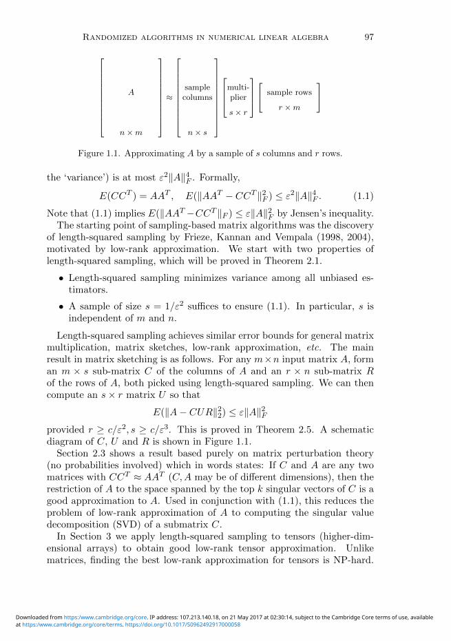
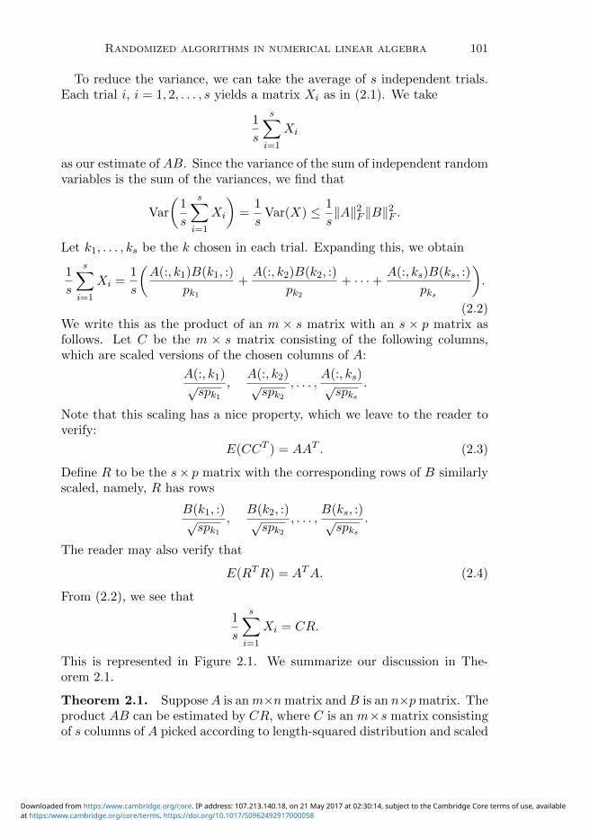
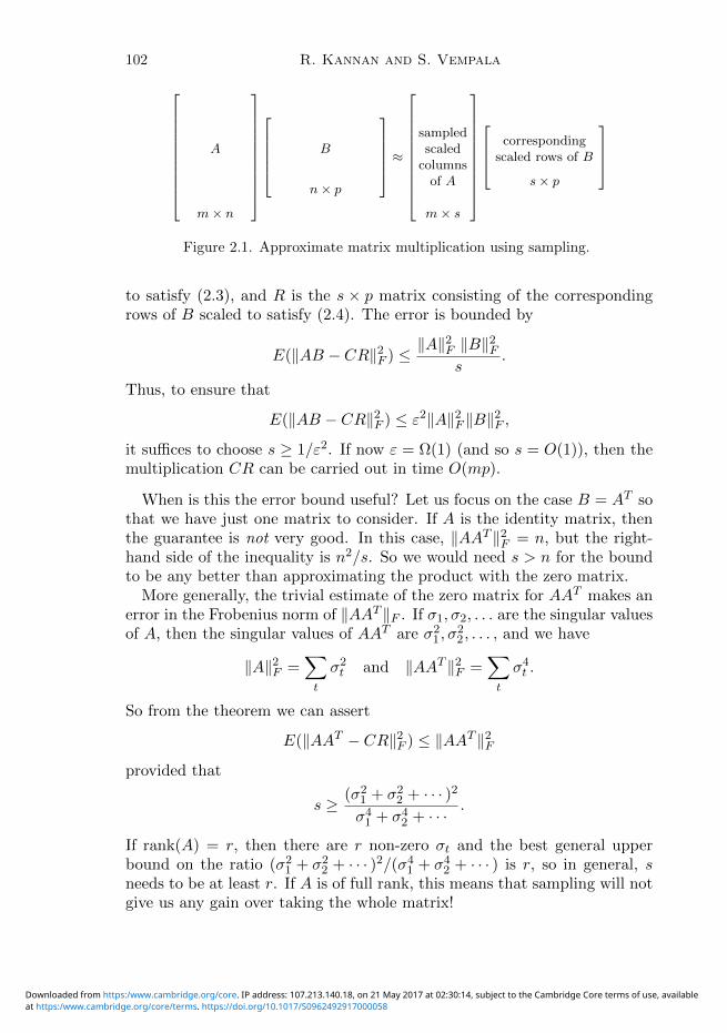