Random Threshold Digraphs

Random Threshold Digraphs

Elizabeth ReillyJohns Hopkins University Applied Physics Laboratory

Laurel, Maryland 20723 [email protected]

Edward Scheinerman Yiguang ZhangApplied Mathematics & Statistics Department

Johns Hopkins UniversityBaltimore, MD 21218 USA

[email protected] [email protected]

Submitted: Jan 22, 2014; Accepted: May 26, 2014; Published: Jun 9, 2014

Mathematics Subject Classification 05C62, 05C80

Abstract

This paper introduces a notion of a random threshold directed graph, extendingthe work of Reilly and Scheinerman in the undirected case and closely related torandom Ferrers digraphs.

We begin by presenting the main definition: D is a threshold digraph provided wecan find a pair of weighting functions f, g : V (D)→ R such that for distinct v, w ∈V (D) we have v → w iff f(v) + g(w) > 1. We also give an equivalent formulationbased on an order representation that is purely combinatorial (no arithmetic). Weshow that our formulations are equivalent to the definition in the work of Cloteaux,LaMar, Moseman, and Shook in which the focus is on the degree sequence, andpresent a new characterization theorem for threshold digraphs.

We then develop the notion of a random threshold digraph formed by choosingvertex weights independently and uniformly at random from [0, 1]. We show thatthis notion of a random threshold digraph is equivalent to a purely combinatorialapproach, and present a formula for the probability of a digraph based on countinglinear extensions of an auxiliary partially ordered set.

We capitalize on this equivalence to develop exact and asymptotic properties ofrandom threshold digraphs such as the number of vertices with in-degree (or out-degree) equal to zero, domination number, connectivity and strong connectivity,clique and independence number, and chromatic number.

Keywords: threshold digraph, random graph

the electronic journal of combinatorics 21(2) (2014), #P2.48 1

1 Introduction

1.1 Notation

In this paper graph exclusively means a simple, undirected graph without loops or multipleedges. We write u ∼ v to denote that uv is an edge.

The term digraph means a strict directed graph without loops or multiple edges in thesame direction, but antiparallel edges (u → v and v → u) may be present. Occasionallywe permit loops in directed graphs in which case we use the phrase looped digraphs—inthat case there can be at most one loop incident with a vertex.

We write |G| to denote the number of vertices and ‖G‖ the number of edges in the[di]graph G.

For a digraph D, its underlying simple graph is denoted simp(D). That is, simp(D)is a simple graph with the same vertex set as D in which u ∼ v if and only if u → v orv → u in D.

If X is some property of a random graph [or digraph] on n vertices, we say that Xholds with high probability provided the probability X holds tends to 1 as n→∞.

For integers n > k > 0 we use this notation for rising and falling factorial:

nk = n(n+ 1)(n+ 2) · · · (n+ k − 1) and nk = n(n− 1)(n− 2) · · · (n− k + 1).

1.2 Background: Undirected (random) threshold graphs

The concept of a threshold graph originates with the following problem [4]. For a subsetof vertices of a graph, A ⊆ V (G), let 1A denote the characteristic vector of that set. Thatis, 1A ∈ Rn (where n = |G|) is a 0-1 vector with 1s corresponding to elements of A and0s in the other coordinates. The question is, can one separate subsets of vertices that areindependent (induce no edges) from those that are not by a linear inequality? That is,we seek a vector w and a threshold t such that

A is an independent set of vertices ⇐⇒ 1A ·w < t.

A graph for which such a linear inequality exists is called a threshold graph.However, for our purposes, we use a different, but equivalent, definition. See [8] and

[10].

Definition 1 (Threshold graph). A graph G is called a threshold graph provided there isa function f : V (G)→ R and a real number t such that for distinct vertices v, w we have

v ∼ w ⇐⇒ f(v) + f(w) > t. (1)

There is no loss of generality in assuming that the values of the weighting function fbe restricted to the unit interval [0, 1] and taking the threshold t to be 1. Furthermore, bygently increasing the values assigned to all vertices, we may assume that equality neverholds in (1).


The values assigned to vertices are often referred to as weights and the function f iscalled a threshold representation of G.

There are a variety of interesting results about threshold graphs but we only mentionthe following characterizations; full details in [10].

Theorem 2. Let G be a simple graph. The following are equivalent.

1. G is a threshold graph.

2. G does not contain any of 2K2, C4, or P4 as an induced subgraph.

3. Assuming n = |G| > 2, G contains a vertex v with d(v) = 0 or d(v) = n − 1 andG− v is a threshold graph.

4. G is uniquely determined by its degree sequence. That is, if H is a graph withV (H) = V (G) and ∀v ∈ V (G), dG(v) = dH(v), then H = G.

An alternative perspective is to begin with a list of weights, and from this list ofweights produce a threshold graph. To this end, let Gn denote the set of all graphs G withvertex set V (G) = [n] = {1, 2, . . . , n}. For a vector x ∈ [0, 1]n let T (x) denote the graphG ∈ Gn in which, for distinct vertices u and v, we have u ∼ v iff xu + xv > 1. Thus T isa mapping from the cube [0, 1]n to the set of all n-vertex labelled graphs Gn. Of course,T (x) is, necessarily, a threshold graph.

We use the transformation T to create a natural model of random threshold graphs.One simply selects a point in x ∈ [0, 1]n uniformly at random and apply T to yield arandom threshold graph; see [11] and [12]. Specifically, we define the random graph Gn

to be a random variable taking values in Gn such that

Pr[Gn = G] = µ[T−1(G)

](2)

where µ is Lebesgue measure. Of course, if G is not a threshold graph, Pr[Gn = G] = 0.In [11, 12] an equivalent, purely combinatorial model for random threshold graphs—

based on creation sequences—provides a route to proving various exact and asymptoticresults about random threshold graphs.

For example, we find that for a threshold graph G ∈ Gn, the expression in (2) may bereplaced by this formula:

Pr[Gn = G] =|Aut(G)|

2n−1n!(3)

where Aut(G) is the automorphism group of G.These combinatorial methods lead to exact results on properties of random threshold

graphs. For example:

Pr [Gn is Hamiltonian] =1

2n−1

(n− 2

b(n− 2)/2c

)∼ 1√

2πn.


1.3 Overview of results

The goal of this paper is to extend the work on random threshold graphs [12] (see also[11]) to directed graphs.

(See also [11] and [13] which consider a variant of the random threshold model forbipartite graphs; such graphs are known as random difference graphs. We also refer thereader to [7] for another approach to random threshold graphs in the context of graphlimits.)

In Section 2 we present a definition of threshold digraph that is a natural extensionof Definition 1. Our definition is quite different from that of [5], but we prove thatthe two definitions are equivalent. Indeed we show that these two definitions are, inturn, equivalent to a third definition that is purely combinatorial. We close with a newcharacterization theorem that links all three definitions.

In Section 3 we introduce a model of random threshold digraphs based on choosing apair of random weights for each vertex. Working directly from this definition is difficult,so we are fortunate to be able to present an equivalent, purely combinatorial model basedon random orders. Calculation of the probability of a digraph becomes equivalent tocounting the number of linear extensions in an auxiliary partially ordered set.

We capitalize on this alternative formulation in Section 4 to derive various exact andasymptotic properties of random threshold digraphs such as these:

• the probability of an edge from one vertex to another, the expected value andvariance of the number of edges, and the asymptotic normality of the number ofedges (suitably rescaled);

• exact results on the number of vertices with in-degree [resp. out-degree] equal tozero, an asymptotic result on the number of isolated vertices, and exact result onthe probability there are no vertices with in-degree or out-degree equal to zero;

• with high probability random threshold digraphs are connected, but strongly con-nected only with probability asymptotic to 1/4 (in which case their diameter is atmost 4);

• asymptotic results on clique and independence number; and

• removing directions from a threshold digraph does not give a threshold graph, butdoes give a perfect graph, and this result enables us to give tight bounds on thechromatic number.

2 Threshold digraphs

2.1 Background on threshold digraphs

The authors of [5] define threshold digraphs to be those directed graphs that are uniquelydetermined by their dual degree sequence. That is, let D be a digraph and let v ∈ V (D).


The out degree of v is the number of edges emanating from v and the in degree is thenumber of edges entering v; these are denoted d+(v) and d−(v) respectively. To say that Dis uniquely determined by its dual degree sequence means that if there is another digraphD′ with V (D′) = V (D) for which

∀v ∈ V (D), d+D(v) = d+D′(v) and d−D(v) = d−D′(v)

then D′ = D. The authors of [5] take this uniqueness property as their definition ofdirected threshold graphs. This is analogous to the final conclusion of Theorem 2.

The main result of [5] includes a forbidden subgraph characterization involving thefollowing two ideas:

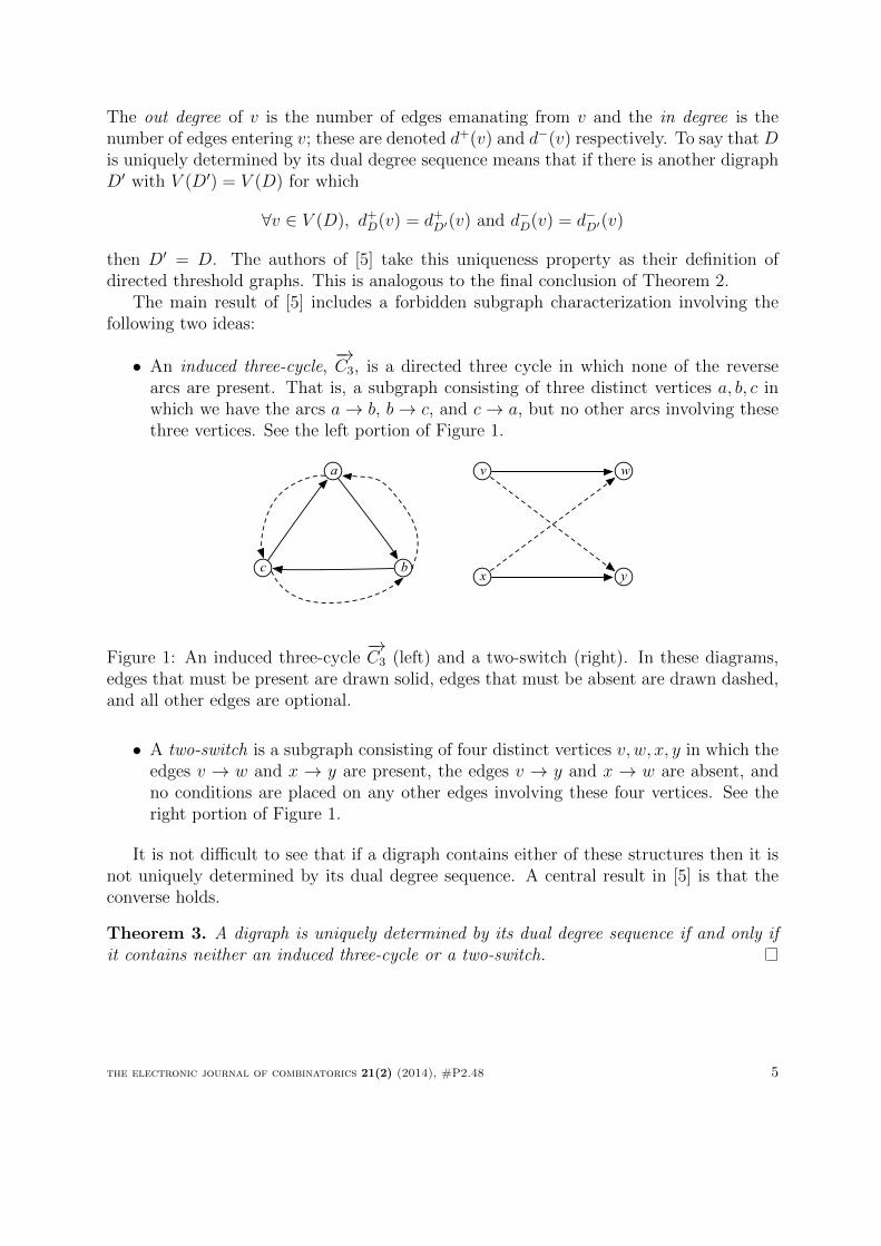
• An induced three-cycle,−→C3, is a directed three cycle in which none of the reverse

arcs are present. That is, a subgraph consisting of three distinct vertices a, b, c inwhich we have the arcs a→ b, b→ c, and c→ a, but no other arcs involving thesethree vertices. See the left portion of Figure 1.

v

yx

wa

bc

Figure 1: An induced three-cycle−→C3 (left) and a two-switch (right). In these diagrams,

edges that must be present are drawn solid, edges that must be absent are drawn dashed,and all other edges are optional.

• A two-switch is a subgraph consisting of four distinct vertices v, w, x, y in which theedges v → w and x → y are present, the edges v → y and x → w are absent, andno conditions are placed on any other edges involving these four vertices. See theright portion of Figure 1.

It is not difficult to see that if a digraph contains either of these structures then it isnot uniquely determined by its dual degree sequence. A central result in [5] is that theconverse holds.

Theorem 3. A digraph is uniquely determined by its dual degree sequence if and only ifit contains neither an induced three-cycle or a two-switch.


2.2 Threshold representation definition

The focus of [5] concerns matters of degree sequences and no consideration is given in thatpaper to representing digraphs by assigning weights to vertices. That is the approach wetake here.

Rather than assigning a single weight to a vertex, we give each vertex a pair of weights:one representing a “send” weight and another being a “receive” weight. (See [16] for ananalogous approach for random dot product digraphs.) There is a directed edge from onevertex to another exactly when the sum of former’s send weight and the latter’s receiveweight is large enough. Here is the formal definition.

Definition 4 (Threshold digraph). Let D be a digraph. We say that D is a thresholddigraph provided there is a pair of functions f, g : V (D) → [0, 1] such that for distinctu, v ∈ V (D) we have

u→ v ⇐⇒ f(u) + g(v) > 1. (4)

The pair (f, g) is called a threshold representation of D. As in the undirected case,there is no loss of generality in assuming that equality does not hold in (4):

u→ v ⇐⇒ f(u) + g(v) > 1 and u 6→ v ⇐⇒ f(u) + g(v) < 1.

In this case, we say that the threshold representation is strict.We check that if D is a threshold digraph then D does not contain an induced three-

cycle or a two switch. Let (f, g) be a threshold representation of D.

• If D contains an induced three-cycle with vertex set a, b, c then we have these in-equalities

f(a) + g(b) > 1 f(b) + g(a) < 1

f(b) + g(c) > 1 f(c) + g(b) < 1

f(c) + g(a) > 1 f(a) + g(c) < 1

giving conflicting inequalities for f(a) + f(b) + f(c) + g(a) + g(b) + g(c).⇒⇐

• Similarly, if D contains a two-switch with vertex set v, w, x, y, then we have

f(v) + g(w) > 1 f(v) + g(y) < 1

f(x) + g(y) > 1 f(x) + g(w) < 1

giving conflicting inequalities for f(v) + f(x) + g(w) + g(y).⇒⇐

In section 2.4 we show that the converse is also true: if D has neither an inducedthree-cycle nor a two-switch, then it is a threshold digraph (our definition).


2.3 Order representations and auxiliary bipartite digraphs

Our characterization of threshold digraphs and later analysis of random threshold digraphsrelies on the following ideas.

Let (f, g) be a strict threshold representation of a threshold digraph D. Observe:

v → w ⇐⇒ f(v) + g(w) > 1 ⇐⇒ f(v) > 1− g(w)v 6→ w ⇐⇒ f(v) + g(w) < 1 ⇐⇒ f(v) < 1− g(w).

Now if we make the following substitutions:

f(v) = f(v) and g(v) = 1− g(v)

then we have v → w ⇐⇒ f(v) > g(w). We use this as a basis for the following definition.

Definition 5. Let D be a directed graph and let L be a linearly ordered set. An orderrepresentation of D is a pair of functions f , g : V (D) → L such that for all distinctv, w ∈ V (D) we have v → w ⇐⇒ f(v) > g(w) and v 6→ w ⇐⇒ f(v) < g(w).

Note: We may assume L = [0, 1].This transformation gives the following.

Proposition 6. A digraph is a threshold digraph if and only if it has an order represen-tation.

This modest alternative characterization of threshold digraphs is key to our subsequentanalysis of random threshold digraphs.

Our next step in showing the equivalence of our concept of threshold digraph withthat of [5] is the following definition.

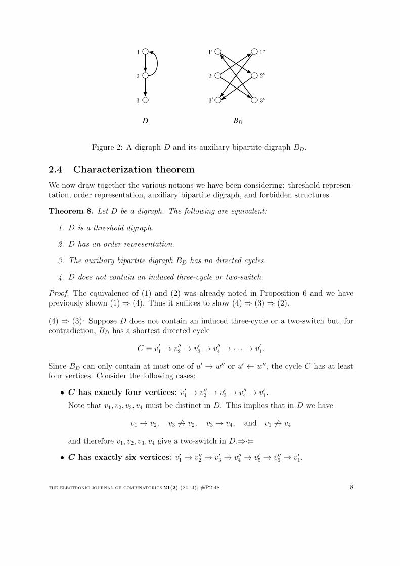
Definition 7. Let D be a digraph with vertex set V . Let V ′ and V ′′ be disjoint copiesof V . That is, to each v ∈ V , there is a v′ ∈ V ′ and a v′′ ∈ V ′′ (and V ′ ∩ V ′′ = ∅).

The auxiliary bipartite digraph of D is a digraph BD with vertex set V ′ ∪ V ′′ in whichwe have exactly these directed edges:

• If v → w in D, then v′ → w′′ in BD.

• If v 6→ w in D, then v′ ← w′′ in BD.

There is never an edge, in either direction, between v′ and v′′ for any v. See Figure 2.

Note that if D has n vertices, then BD has n(n − 1) edges as there is always exactlyone edge between v′ and w′′ for all v 6= w; it is only the direction of the edge between v′

and w′′ that is determined by the presence (or absence) of v → w in D.Observe that for a threshold digraph D, the auxiliary bipartite digraph BD encapsu-

lates the order representation:

v → w ⇐⇒ f(v) > g(w) ⇐⇒ v′ → w′′

v 6→ w ⇐⇒ f(v) < g(w) ⇐⇒ v′ ← w′′

Of course, BD is defined for arbitrary digraphs D, so we need to sort out the difference.


1� 1��1

2 2� 2��

3 3� 3��

D BD

Figure 2: A digraph D and its auxiliary bipartite digraph BD.

2.4 Characterization theorem

We now draw together the various notions we have been considering: threshold represen-tation, order representation, auxiliary bipartite digraph, and forbidden structures.

Theorem 8. Let D be a digraph. The following are equivalent:

1. D is a threshold digraph.

2. D has an order representation.

3. The auxiliary bipartite digraph BD has no directed cycles.

4. D does not contain an induced three-cycle or two-switch.

Proof. The equivalence of (1) and (2) was already noted in Proposition 6 and we havepreviously shown (1)⇒ (4). Thus it suffices to show (4)⇒ (3)⇒ (2).

(4) ⇒ (3): Suppose D does not contain an induced three-cycle or a two-switch but, forcontradiction, BD has a shortest directed cycle

C = v′1 → v′′2 → v′3 → v′′4 → · · · → v′1.

Since BD can only contain at most one of u′ → w′′ or u′ ← w′′, the cycle C has at leastfour vertices. Consider the following cases:

• C has exactly four vertices: v′1 → v′′2 → v′3 → v′′4 → v′1.

Note that v1, v2, v3, v4 must be distinct in D. This implies that in D we have

v1 → v2, v3 6→ v2, v3 → v4, and v1 6→ v4

and therefore v1, v2, v3, v4 give a two-switch in D.⇒⇐

• C has exactly six vertices: v′1 → v′′2 → v′3 → v′′4 → v′5 → v′′6 → v′1.


– Subcase: These six BD vertices correspond to exactly three vertices in D.

In this case, the cycle C must be of the form

a′ → b′′ → c′ → a′′ → b′ → c′′ → a′

where a, b, c are distinct. This implies that in D we have a → b → c → a buta 6→ c 6→ b 6→ a; that is, D contains an induced three-cycle.⇒⇐

– Subcase: These six BD vertices correspond to four or more vertices of D.

In this case, we have v1 6= v4, v2 6= v5, or v3 6= v6; without loss of generality,say v1 6= v4. Therefore either v′1 → v′′4 or v′1 ← v′′4 in BD. In the first case BD

has the cycle v′1 → v′′4 → v′5 → v′′6 → v′1 and in the second case BD has thecycle v′1 → v′′2 → v′3 → v′′4 → v′1, contradicting the fact that C is a shortestdirected cycle in BD.⇒⇐

• C has exactly eight or more vertices.

In this case v1 6= v4 or v1 6= v6. This implies that one of v′1 → v′′4 , v′1 ← v′′4 , v′1 → v′′6 ,or v′1 ← v′′6 is an edge of BD and, as before, we find a directed cycle shorter thanC.⇒⇐

Therefore BD does not contain a directed cycle.

(3)⇒ (2): Suppose BD has no directed cycle.Since BD is a directed acyclic graph, let L be a topological sort of its vertices. That

is, L is a linear order with the property that if α→ β in BD, then α > β in L.Define functions f , g : V (D)→ L by

f(v) = v′ and g(v) = v′′

and observe that this is an order representation of D.

3 Random model

We now develop a model of random threshold digraphs based on random representations,but also provide an equivalent, purely combinatorial formulation.

In general, a random threshold digraph is a random variable Dn taking values in Dn:the set of all digraphs D with V (D) = [n] = {1, 2, . . . , n}.

3.1 Random representation

Let n be a positive integer. Informally, we create a random threshold digraph Dn by se-lecting 2n random numbers X1, X2, . . . , Xn, Y1, Y2, . . . , Yn chosen independently and uni-formly from [0, 1]. We use these to construct a digraph D with V (D) = [n] in whichu→ v exactly when Xu + Yv > 1.

More formally, we define a mapping from the cube [0, 1]2n to Dn and create a randomthreshold digraph by choosing a point from the cube. We start with this definition.


Definition 9. Let n be a positive integer. Define T : [0, 1]n × [0, 1]n → Dn as follows.Let T (x,y) be the digraph D with V (D) = [n] and for distinct u, v ∈ [n] we have u→ viff xu + yv > 1.

We have presented this representation function T as depending on two argumentsx,y ∈ [0, 1]n but, of course, we may also think of it as a function of a single 2n-longvector formed by concatenating x and y, or as n points (xi, yi) in the unit square [0, 1]2.

Next we define the random threshold digraph Dn to be the random variable takingvalues in Dn such that

Pr [Dn = D] = µ[T−1(D)

]where µ is Lebesgue measure.

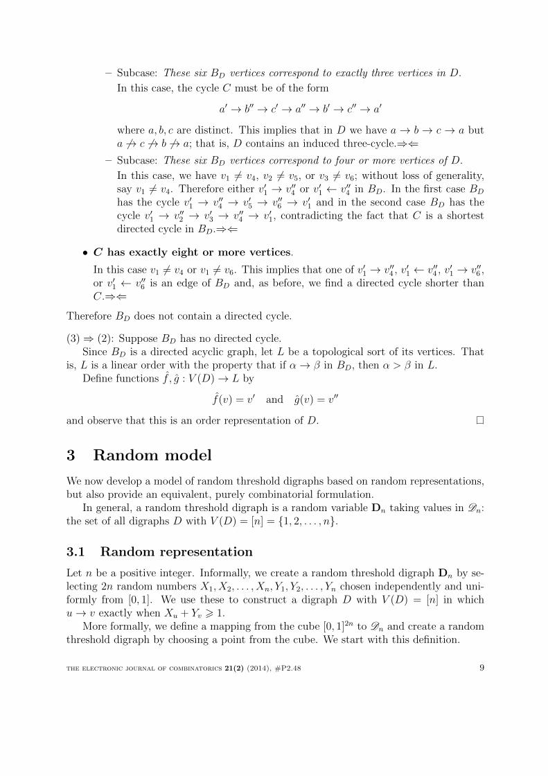
For example, let D be the digraph in Figure 3. To calculate its probability, we need

Figure 3: A threshold digraph D for which the probability D3 = D is 1/180.

to find the volume of the subset of [0, 1]6 consisting of those points (x1, x2, x3, y1, y2, y3)for which all of the following hold:

x1 + y2 > 1 x1 + y3 < 1 x2 + y3 > 1

x2 + y1 > 1 x3 + y1 < 1 x3 + y2 < 1.

The infinitely patient reader can cast this problem as the sum of these three six-foldintegrals: ∫ 1

0

dy2

∫ y2

0

dy3

∫ y3

0

dy1

∫ 1−y3

1−y2dx1

∫ 1

1−y1dx2

∫ 1−y2

0

dx3 =1

720∫ 1

0

dy2

∫ y2

0

dy3

∫ y3

0

dy1

∫ 1−y3

1−y2dx1

∫ 1

1−y1dx2

∫ 1−y2

0

dx3 =1

720∫ 1

0

dy2

∫ y2

0

dy1

∫ y1

0

dy3

∫ 1−y3

1−y2dx1

∫ 1

1−y3dx2

∫ 1−y2

0

dx3 =1

360

and conclude Pr[D3 = D] = 1/180. There’s got to be a better way!

3.2 A combinatorial approach

Defining random threshold digraphs by choosing a random threshold representation isnatural, but computationally challenging. Here we show that by choosing a random order


representation gives an equivalent notion of random threshold digraph that is far moretractable.

The key idea is to replace the random point (x,y) ∈ [0, 1]2n with the random point(x, y), also in [0, 1]2n, where

xj = xj and yj = 1− yj.

Note that if the point (x,y) is chosen uniformly at random in [0, 1]2n, the same is truefor (x, y). Furthermore, with probability one, the 2n values x1, . . . , yn are distinct. And,of course,

xu + yv > 1 ⇐⇒ xu > yv and xu + yv < 1 ⇐⇒ xu < yv.

The cube [0, 1]2n can be dissected into (2n)! congruent regions based on the order of the2n coordinates. To find the probability Dn is a particular threshold digraph D, we justcount the number of distinct order representations and divide by (2n)!.

More formally, consider the (2n)! linear orders of the symbols 1′, 2′, . . . , n′, 1′′, 2′′, . . . , n′′.Let L be such a linear order and define T (L) to be the digraph in Dn in which v → wwhen v′ > w′′ (and v 6→ w when v′ < w′′).

We therefore can conclude that Pr[Dn = D] equals the number of linear orders L withT (L) = D, divided by (2n)!.

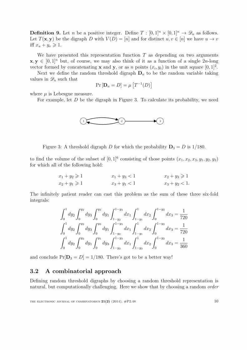
We can say a bit more. Recall the auxiliary bipartite digraph BD from Definition 7.

Definition 10 (Auxiliary poset). Let D be a threshold digraph with vertex set V andlet BD be its auxiliary bipartite digraph with vertex set V ′ ∪ V ′′. The auxiliary partiallyordered set PD has ground set V ′ ∪ V ′′ and for α, β ∈ V ′ ∪ V ′′ we have α > β exactlywhen there is a directed path from α to β in BD.

Note that for threshold digraphs, BD is acyclic and therefore the relation defined inDefinition 10 indeed gives a poset. See Figure 4 for an example.

1� 1��

2� 2��

3� 3��

BD PD

1�1��

2�

2��

3�

3��1

2

3

D

Figure 4: The auxiliary digraph BD and auxiliary poset PD for the digraph D fromFigure 3.


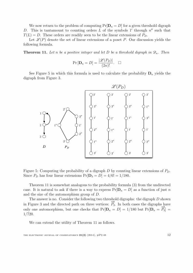
We now return to the problem of computing Pr[Dn = D] for a given threshold digraphD. This is tantamount to counting orders L of the symbols 1′ through n′′ such thatT (L) = D. These orders are readily seen to be the linear extensions of PD.

Let L (P ) denote the set of linear extensions of a poset P . Our discussion yields thefollowing formula.

Theorem 11. Let n be a positive integer and let D be a threshold digraph in Dn. Then

Pr [Dn = D] =|L (PD)|

(2n)!.

See Figure 5 in which this formula is used to calculate the probability Dn yields thedigraph from Figure 3.

PD

1�1��

2�

2��

3�

3��

3� 3� 3� 3�

2��2��2��

2��

1��

1��

1��

1��

1�

1�1�

1�

3�� 3�� 3��

3��

2� 2� 2� 2�

1

2

3

D

L (PD)

Figure 5: Computing the probability of a digraph D by counting linear extensions of PD.Since PD has four linear extensions Pr[D3 = D] = 4/6! = 1/180.

Theorem 11 is somewhat analogous to the probability formula (3) from the undirectedcase. It is natural to ask if there is a way to express Pr[Dn = D] as a function of just nand the size of the automorphism group of D.

The answer is no. Consider the following two threshold digraphs: the digraph D shown

in Figure 3 and the directed path on three vertices:−→P3. In both cases the digraphs have

only one automorphism, but one checks that Pr[Dn = D] = 1/180 but Pr[Dn =−→P3] =

1/720.

We can extend the utility of Theorem 11 as follows.


Theorem 12. Let X be any property of directed graphs. The probability Dn has propertyX equals the number of orders L of 1′, 2′, . . . , n′, 1′′, 2′′, . . . , n′′ such that T (L) has propertyX , divided by (2n)!.

While the formula presented in Theorem 11 is simple and makes the problem of cal-culating Pr[Dn = D] feasible, it is not clear how useful this formula is for large digraphs.In particular, it is known that the problem of counting the linear extensions of a generalposet is #P-complete [2]. However, the posets PD arise in a rather special way and it isconceivable that an efficient (polynomial time) algorithm for calculating Pr[Dn = D] mayexist. We leave this as an open question:

Question 13. What is the computational complexity of calculating the probability thatDn takes on a particular value. That is, consider this problem:

• Instance: A directed graph D on n vertices.

• Evaluate: (2n)! Pr[Dn = D].

Is this problem #P-complete?

Note that the corresponding problem for (undirected) threshold graphs is polynomialtime computable because the calculation of |Aut(G)| is easy in the case G is threshold.

3.3 Examples

Here we calculate the probability Dn is an edgeless digraph and a complete bipartitedigraph.

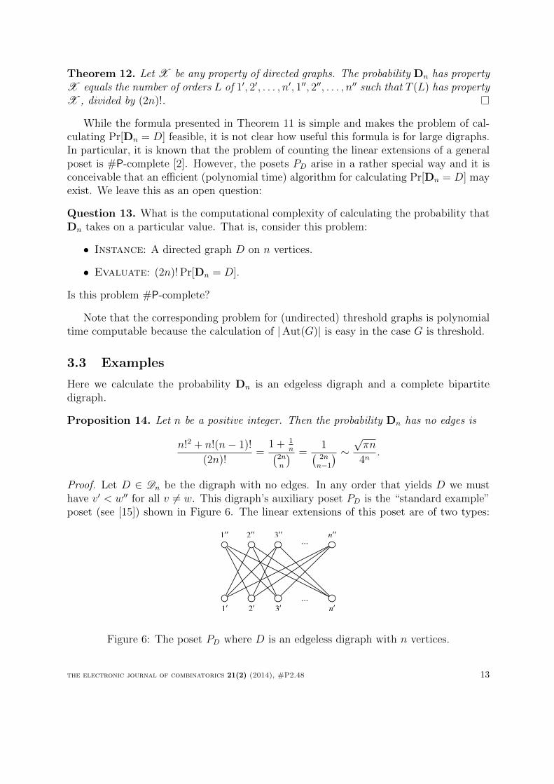
Proposition 14. Let n be a positive integer. Then the probability Dn has no edges is

n!2 + n!(n− 1)!

(2n)!=

1 + 1n(

2nn

) =1(2nn−1

) ∼ √πn4n

.

Proof. Let D ∈ Dn be the digraph with no edges. In any order that yields D we musthave v′ < w′′ for all v 6= w. This digraph’s auxiliary poset PD is the “standard example”poset (see [15]) shown in Figure 6. The linear extensions of this poset are of two types:

10

100 200

20 30

300 n00

n0…

…

Figure 6: The poset PD where D is an edgeless digraph with n vertices.


one in which all v′ elements are below all w′′ elements, and one in which a single u′ isabove its corresponding u′′, like this:

v′1 < v′2 < · · · < v′n−1 < u′′ < u′ < w′′1 < w′′2 < · · · < w′′n−1.

There are (n!)2 linear extensions of the first kind and n · (n− 1)!2 linear extensions of thesecond kind. The result now follows by Theorem 11.

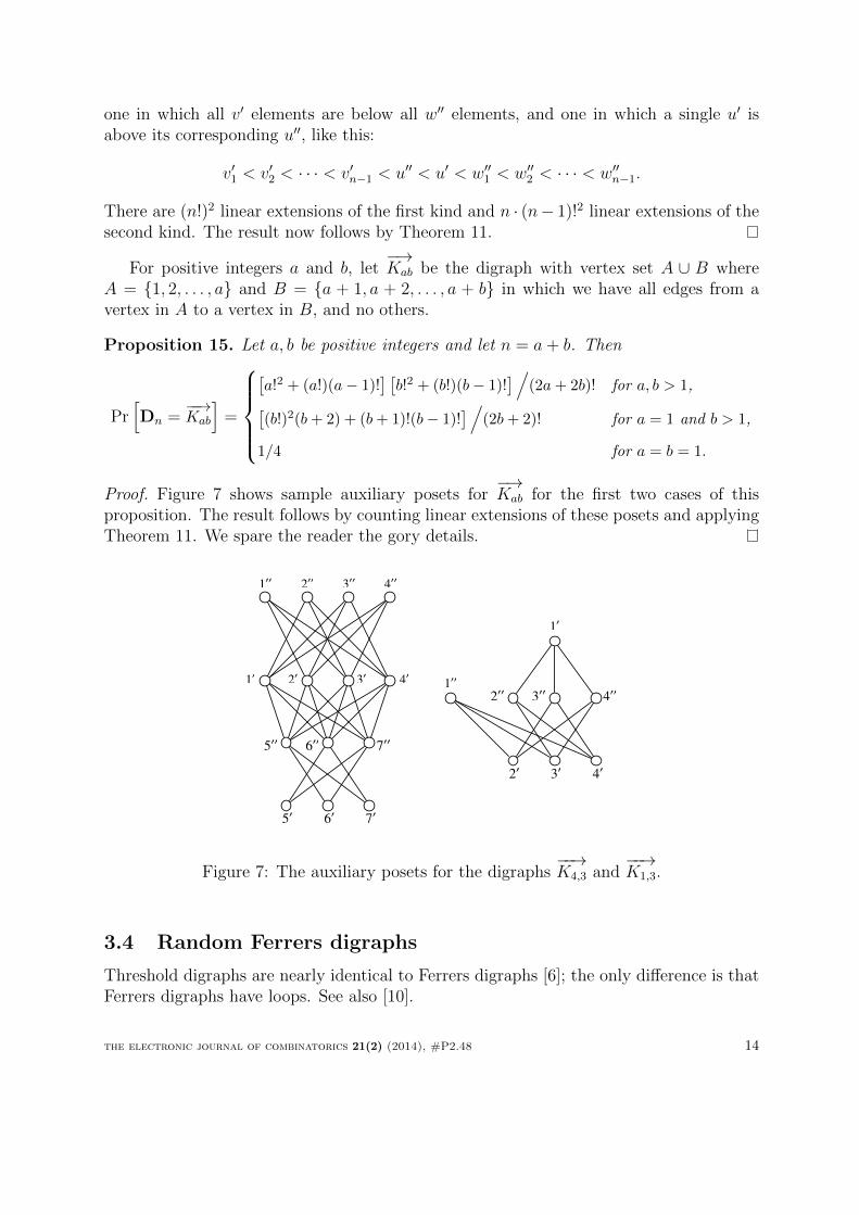
For positive integers a and b, let−→Kab be the digraph with vertex set A ∪ B where

A = {1, 2, . . . , a} and B = {a + 1, a + 2, . . . , a + b} in which we have all edges from avertex in A to a vertex in B, and no others.

Proposition 15. Let a, b be positive integers and let n = a+ b. Then

Pr[Dn =

−−→Kab

]=

[a!2 + (a!)(a− 1)!

] [b!2 + (b!)(b− 1)!

]/(2a + 2b)! for a, b > 1,[

(b!)2(b + 2) + (b + 1)!(b− 1)!]/

(2b + 2)! for a = 1 and b > 1,

1/4 for a = b = 1.

Proof. Figure 7 shows sample auxiliary posets for−→Kab for the first two cases of this

proposition. The result follows by counting linear extensions of these posets and applyingTheorem 11. We spare the reader the gory details.

1�

1��

2� 3� 4�

2�� 3�� 4��1�

1�� 2��

2� 3�

3�� 4��

4�

5� 6� 7�

5�� 6�� 7��

Figure 7: The auxiliary posets for the digraphs−−→K4,3 and

−−→K1,3.

3.4 Random Ferrers digraphs

Threshold digraphs are nearly identical to Ferrers digraphs [6]; the only difference is thatFerrers digraphs have loops. See also [10].


Definition 16. Let D be a looped digraph. We say that D is a Ferrers digraph providedthere are functions f, g : V (D) → [0, 1] such that for all v, w ∈ V (D) we have v → w ifff(v) + g(w) > 1.

If we are given a Ferrers digraph D and remove the loops from D, the result is athreshold digraph. That raises the question: Given a threshold digraph D, how can weplace loops on the vertices so that the resulting digraph is a Ferrers digraph? That is, onwhich vertices should we place loops to convert D into a Ferrers digraph?

One can check that the following works. Assume V (D) = [n] and find all linearextensions of PD. For a given linear extension L, place a loop on a vertex v exactly whenv′ > v′′ to give a Ferrers digraph. Stepping through the various linear extensions of PD

will generate all possible Ferrers digraphs formed by adding loops to D.For example, consider the digraph D in Figure 3; its auxiliary poset PD has four linear

extensions as shown in Figure 5. In all four extensions we have 3′ < 3′′ and 2′ > 2′′, butin some 1′ < 1′′ and in others 1′ > 1′′. This implies that there exactly two ways to addloops to D to make it a Ferrers digraph: add loops to both vertices 1 and 2, or have aloop only at vertex 2.

A study of random Ferrers digraphs is presented in [11]. The fundamental ideas arethe same. Let Fn denote the set of all looped digraphs with vertex set [n]. For (x,y) ∈[0, 1]n × [0, 1]n, let F (x,y) be the looped digraph in Fn in which i → j iff xi + yj > 1.Define the random variable Fn, taking values in Fn, with Pr [Fn = D] = µ [F−1(D)]. In[11] a combinatorial formulation (patterned after creation sequences) provides a tool forthe analysis of these random digraphs.

A simple relation connects Fn and Dn. For a digraph D ∈ Dn, let `(D) denote the setof all possible looped digraphs we can form by adding loops to D. Thus `(D) contains 2n

looped digraphs. For D ∈ Dn we have

Pr [Dn = D] =∑

D′∈`(D)

Pr [Fn = D′] .

(The left side implicitly counts all orders L such that T (L) = D; the right side counts thesame orders but separates cases in which v′ < v′′ versus v′ > v′′ depending on whether ornot there is a loop at v.)

Thus, if some property X holds with high probability for random Ferrers digraphs,it follows that X holds with high probability for random threshold digraphs.

4 Results

4.1 Edges and degrees

It is easy to check that the probability there is an edge from one vertex to another in arandom threshold digraph is 1

2and that edges u→ v and v → u are independent. Further,

if u, v, x, y are distinct vertices, the edges u → v and x → y are independent. However,in contrast to Erdos-Renyi random graphs, there are dependencies between edges. Thisfirst result illustrates the use of Theorem 12.


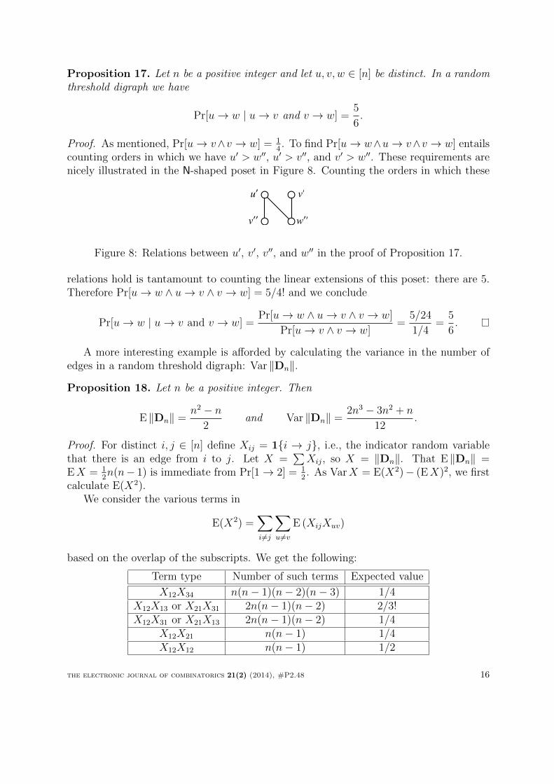
Proposition 17. Let n be a positive integer and let u, v, w ∈ [n] be distinct. In a randomthreshold digraph we have

Pr[u→ w | u→ v and v → w] =5

6.

Proof. As mentioned, Pr[u→ v∧v → w] = 14. To find Pr[u→ w∧u→ v∧v → w] entails

counting orders in which we have u′ > w′′, u′ > v′′, and v′ > w′′. These requirements arenicely illustrated in the N-shaped poset in Figure 8. Counting the orders in which these

u�

w��v��

v�

Figure 8: Relations between u′, v′, v′′, and w′′ in the proof of Proposition 17.

relations hold is tantamount to counting the linear extensions of this poset: there are 5.Therefore Pr[u→ w ∧ u→ v ∧ v → w] = 5/4! and we conclude

Pr[u→ w | u→ v and v → w] =Pr[u→ w ∧ u→ v ∧ v → w]

Pr[u→ v ∧ v → w]=

5/24

1/4=

5

6.

A more interesting example is afforded by calculating the variance in the number ofedges in a random threshold digraph: Var ‖Dn‖.

Proposition 18. Let n be a positive integer. Then

E ‖Dn‖ =n2 − n

2and Var ‖Dn‖ =

2n3 − 3n2 + n

12.

Proof. For distinct i, j ∈ [n] define Xij = 1{i → j}, i.e., the indicator random variablethat there is an edge from i to j. Let X =

∑Xij, so X = ‖Dn‖. That E ‖Dn‖ =

EX = 12n(n− 1) is immediate from Pr[1→ 2] = 1

2. As VarX = E(X2)− (EX)2, we first

calculate E(X2).We consider the various terms in

E(X2) =∑i 6=j

∑u6=v

E (XijXuv)

based on the overlap of the subscripts. We get the following:

Term type Number of such terms Expected value

X12X34 n(n− 1)(n− 2)(n− 3) 1/4X12X13 or X21X31 2n(n− 1)(n− 2) 2/3!X12X31 or X21X13 2n(n− 1)(n− 2) 1/4

X12X21 n(n− 1) 1/4X12X12 n(n− 1) 1/2


Note: The calculation of E(X12X13) follows from the requirement that we have 1′ > 2′′

and 1′ > 3′′. There are 3! orders for the symbols 1′, 2′′, and 3′′ of which exactly two yieldthe 1→ 2 and 1→ 3.

Adding the terms in the chart and subtracting (EX)2 gives the result.

If the edges of a random threshold digraph were mutually independent (as in Erdos-Renyi graphs) then the variance would be on the order of n2; the higher variance is dueto the edge dependencies. And if the edges were mutually independent, then the numberof edges would converge to a normal distribution. Despite dependencies, the same holdsfor random threshold digraphs.

Theorem 19. Let n be a positive integer and set µn = E ‖Dn‖ and σ2n = Var ‖Dn‖. Then

‖Dn‖ − µn

σn

converges in distribution to a standard normal random variable.

Proof. The number of edges in a random threshold digraph is readily seen to be a U-statistic and convergence to normality follows from a result of Hoeffding [9]. See Theo-rem 5.5.1A in [14].

In an Erdos-Renyi random graph, vertex degrees are highly concentrated near theaverage degree. By contrast, the in- and out-degrees of vertices in Dn are uniformlydistributed between 0 and n− 1 as shown in the next proposition.

Proposition 20. Let n, k be integers with 0 6 k < n. For a given vertex v, the probabilityd+(v) = k is 1/n.

Proof. Consider the out-degree of vertex 1 in Dn. Consider the n! orders of the n symbols1′ and 2′′, 3′′, . . . , n′′. There are (n − 1)! ways to order the symbols 2′′, . . . , n′′ and thenexactly one way to insert 1′ into that order so that d+(1) = k. Therefore Pr[d+(1) = k] =(n− 1)!/n! = 1/n.

It’s easy to check that, for a given vertex v, the in-degree and out-degree of v areindependent. Therefore, the probability that a vertex of Dn is isolated is 1/n2. Thereforethe expected number of isolated vertices in Dn is 1/n and Markov’s inequality gives thefollowing result.

Proposition 21. With high probability, Dn has no isolated vertices.

This result suggests that, with high probability, Dn is connected. We explore thisissue in Section 4.3.

While it is unlikely for a vertex to have both in- and out-degree equal to zero, we mayhave one of these be zero and here we present some results in that regard.

We call a vertex v with out-degree d+(v) = 0 a sink and a vertex with d−(v) = 0 iscalled a source.


Proposition 22. Let n > 2. The probability that Dn has no sinks is 12− 1

2n. The

probability it has exactly k sinks, where 1 6 k 6 n, is

(n+ 1)k+1

(2n)k+1.

Note that if k = n, then Dn has no edges and the formula in Proposition 22 reduces

to(

2nn−1

)−1which agrees with Proposition 14.

Proof. First we count the number of orders L of 1′, . . . , n′, 1′′, . . . , n′′ such that the resultingdigraph T (L) has no sinks. This requires that for every u ∈ [n] there is a v ∈ [n] withv 6= u such that u′ > v′′; this ensures that u has at least one out-neighbor.

Without loss of generality, we assume that elements 1′′ through n′′ are in the order1′′ < 2′′ < · · · < n′′; we multiply by n! at the end to account for other possibilities.

Into this we can insert element 1′ anywhere above 2′′ (otherwise 1′ is a sink); there aren− 1 such choices.

Next insert elements 2′ through n′ into this list of n + 1 elements anywhere above 1′′

(for otherwise the inserted element would be a sink). The number of ways to add theseelements to the order is (n+ 1)n−1.

Therefore, probability Dn has no sink is

n!(n− 1)(n+ 1)n−1

(2n)!=

1

2− 1

2n.

Next we count orders of the 2n symbols 1′ through n′′ that produce a threshold digraphwith exactly k sinks. As before, we only consider orders with 1′′ < 2′′ < · · · < n′′ andmultiply by n! at the end.

Let L be such an order and let S be the set of k sinks in T (L). We consider the cases1 /∈ S and 1 ∈ S separately.

Case I: 1 /∈ S. There are(n−1k

)choices for this set.

Let the n − k non-sink elements be 1, u2, u3, . . . , un−k. We first insert the elements1′, u′2, u

′3, . . . , u

′n−k into the order 1′′ < 2′′ < · · · < n′′. Starting with 1′, we note that we

must have 1′ > 2′′ for otherwise 1 would be a sink; there are n− 1 choices for its insertionpoint.

The remaining elements u′2 through u′n−k may be inserted anywhere above element1′′ (because placing u′′j < 1′′ would make uj a sink); the number of ways to insert these

elements is therefore (n+ 1)n−k−1.

Therefore there are (n − 1)(n + 1)n−k−1 ways to insert the nonsinks into the order1′′ < 2′′ < · · · < n′′.

Finally, we insert k symbols s′ for s ∈ S. Because these are sinks, they must all bebelow 1′′, but in any order. This gives k! choices. Therefore the number of orderings inthis case (1 /∈ S) is (

n− 1

k

)k!(n− 1)(n+ 1)n−k−1. (5)


Case II: 1 ∈ S. There are(n−1k−1

)choices for this set. We separately count the orders in

which 1′ < 1′′ and in which 1′ > 1′′.Subcase (a): 1′ < 1′′.

We have 1′ < 1′′ < 2′′ < · · · < n′′. For s ∈ S with s 6= 1 we must have s′ < 1′′

(otherwise we have the arc s→ 1). In other words, the elements of S appearin any order below 1′′, and there are k! ways that can happen.

Having inserted all the elements s′ with s ∈ S into the order, we now insertthe remaining n− k elements v′. Necessarily these must lie above 1′′ (because

they are not sinks) and there there are nn−k ways to do this.

Thus the number of orders in this subcase is k!nn−k.

Subcase (b): 1′ > 1′′.

Since 1 is a sink, 1′ cannot be above 2′′ and so we must have 1′′ < 1′ < 2′′ <3′′ < · · · < n′′. For the other elements s ∈ S we must have s′ < 1′′ (or else sis not a sink) and these may lie there in any order. Hence there are (k − 1)!ways to insert these elements.

Next we insert the elements v′ for v /∈ S into the order. These elements mustbe above 1′′ (or else they are sinks) but may lie on either side of 1′. The

number of ways to insert these elements is (n+ 1)n−k.

Thus there are (k − 1)!(n+ 1)n−k orders in this subcase.

We now combine these subcases, multiply by(n−1k−1

)for the choices for the set S, and

find that the number of orders in Case II is(n− 1

k − 1

)[k!nn−k + (k − 1)!(n+ 1)n−k

]. (6)

Finally, we add (5) and (6), multiply by n! (for the orders of 1′′, 2′′, . . . , n′′), divide by(2n)!, and simplify to get the result.

Corollary 23. For all n > 1, the expected number of sinks in Dn is 1. Furthermore, fora given nonnegative integer k we have

limn→∞

Pr [Dn has exactly k sinks] =1

2k+1.

In section 4.3 we examine the probability that Dn is strongly connected. A digraphthat has a source or a sink cannot be strongly connected. Proposition 22 shows that theprobability Dn has no sinks is asymptotically 1

2; the same is true, of course, for sources.

If having no sinks and having no sources were independent, then it would be a simplematter to conclude that the probability Dn has neither is asymptotically 1

4. This is so,

but it takes more work.


Proposition 24. Let n > 2 be an integer. The probability that Dn has no sinks and nosources is

n3 − 3n2 + 5n− 2

2n(2n− 1)(n− 1)− (n− 1)!(n− 2)!

2(2n− 1)!

which converges to 14

as n→∞.

Proof. We consider the orders for 1′, . . . , n′′ that yield threshold digraphs without sourcesor sinks.

In such an order, the least element must not be of the form v′ for then v would haveno outgoing edges. Likewise, the greatest element cannot be of the form v′′. Therefore,the relevant orders must be of the form v′′ < · · · < w′ where we might have v = w orv 6= w; these are mutually exclusive cases that we consider separately.

In case v = w, the order is of the form v′′ < · · · < v′; call this event A1. Notice that inthis case, vertex v has edges to and from every other vertex and so there are no sourcesand no sinks. We have

Pr(A1) =n(2n− 2)!

(2n)!=

1

4n− 2.

The case v 6= w is more complicated. Let A2 be the event that the order is of the formv′′ < · · · < w′ with v 6= w. We have

Pr(A2) =n(n− 1)(2n− 2)!

(2n)!=

n− 1

4n− 2.

Without loss of generality, we examine the case 1′′ < · · · < n′.Notice for a vertex x with 1 < x < n we already have x → 1 and n → x. Thus x is

neither source nor sink, 1 is not a source, and n is not a sink.

• To ensure that 1 is not a sink, we must not have

1′ < 2′′, 3′′, . . . , n′′︸︷︷︸any order

.

We call this obstruction B1 and we have

Pr(B1) =(n− 1)!

n!=

1

n.

• To ensure that n is not a source, we must not have

1′, 2′, . . . , (n− 1)′︸︷︷︸any order

< n′′.

We call this obstruction B2 and Pr(B2) = 1/n also.


Combining these cases we have that the probability that Dn has no source and no sinkis precisely Pr(A1) + Pr(A2) Pr(B1 ∪B2). Since Pr(B1 ∪B2) = 1 − Pr(B1) − Pr(B2) +Pr(B1 ∩B2) we work to calculate Pr(B1 ∩B2).

Since B1 holds, we have 1′ < [2′′, 3′′, . . . , n′′] and we condition on the location of n′′:in this list of n symbols, it might be in position 2, 3, . . . , or n. Suppose it is in the kth

position:1′ <?′′2 <?′′3 < · · · <?′′k−1 < n′′ <?′′k+1 < · · · <?′′n.

The number of ways this can happen is (n−2)!. We now insert the symbols 2′, 3′, . . . , (n−1)′ ensuring that all of these are less than n′′ (as required by B2). The number of waysto do this is k(k + 1)(k + 2) . . . (k + n− 3) = kn−2. Thus

Pr(B1 ∩B2) =(n− 2)!

(2n)!

n∑k=2

kn−2 =(n− 2)!

(2n)!· (2n− 2)!− (n− 1)!2

(n− 1)(n− 1)!.

Substituting these into Pr(A1) + Pr(A2)P (B1 ∪B2) gives the results claimed.

4.2 Domination

Definition 25. Let D be a digraph. A set of vertices S ⊆ V (D) is an out-dominatingset provided for every vertex v either (a) v ∈ S or (b) there is a vertex w ∈ S such thatw → v.

The smallest size of an out dominating set is called the out-domination number of Dand is denoted γ+(D).

Proposition 26. Let n, k be integers with n > k > 1. Then

Pr[γ+(Dn) = k

]=

nk

(2n− 1)k.

Proof. We count the orders of 1′, . . . , n′′ that give rise to digraphs D with γ+(D) = k.We consider the location of the last (i.e., greatest) single-primed element v′. There aretwo possibilities: (a) none of the double-primed elements above v′ is v′′ and (b) one of thedouble-primed elements above v′ is v′′. These two cases look like this:

(a): other elements < v′ < w′′1 , w′′2 , . . . , w

′′k−1︸︷︷︸

any order

(b): other elements < v′ < w′′1 , w′′2 , . . . , w

′′k−1, v

′′︸︷︷︸any order

The number of orders of type (a) is nk−1(n− k+ 1)(2n− k)! and the number of orders oftype (b) is nk · k · (2n− k − 1)!. Adding these and dividing by (2n)! gives the result.

Corollary 27. E [γ+(Dn)] = 2n/(n+ 1) and limn→∞ P [γ+(Dn) = k] = 2−k.


We can consider the domination number of the underlying simple graph of randomthreshold digraph: γ [simp(Dn)]. Computer experiments suggest that with high proba-bility simp(Dn) contains a vertex of degree n− 1, that is, a vertex adjacent to all others.In this case, the domination number equals 1 and we pose this as an open problem.

Conjecture 28. With high probability simp(Dn) contains a vertex adjacent to all others.

Note that this conjecture stands in a bit of contrast to the fact that, with high prob-ability, simp(Dn) does not contain a vertex of degree 0.

4.3 Connectivity

We have seen that the probability Dn has an isolated vertex is vanishingly small (Propo-sition 21) and that the probability Dn has no sources or sinks is asymptotically 1/4(Proposition 24). This suggests—and, in fact, it is the case—that with high probabilityDn is connected, but the probability it is strongly connected tends to 1/4 as n→∞.

Proposition 29. With high probability simp (Dn) is connected.

Proof. Let D be a digraph with vertex set V . We know that simp(D) is not connected iffthere is a subset of vertices A (with A 6= ∅ and A 6= V ) such that there are no directededges in D between A or V − A (in either direction).

For a fixed A of size a, the probability that there are no arcs from A to V − A isa!(n− a)!/n! because in an order representation all v ∈ A and w ∈ V − A we must havev′ < w′′.

Let XA be the indicator random variable that there are no arcs between A and V −A.Since the arcs from A to V − A are independent of the arcs from V − A to A, we have

P (XA = 1) =(na

)−2.

Note that simp(Dn) is connected iff X =∑XA = 0, where the sum is over all

nonempty proper subsets of V . Therefore

Pr [simp(Dn) is not connected] = Pr(X > 0) 6 E(X) =∑A

XA =n−1∑a=1

(n

a

)/(n

a

)2

=n−1∑a=1

1(na

) =2

n+

n−2∑a=2

1(na

) < 2

n+

n(n2

) = O(1/n)→ 0

as n→∞.

We now turn to the question of strong connectivity. There is, asymptotically, onlya 25% chance that Dn has no sources or sinks, and that puts an upper bound on theprobability Dn is strongly connected. For the lower bound, we have the following.

Proposition 30. For n > 3, the probability that Dn is strongly connected with diameterat most 4 is at least

1

4n− 2+

n− 1

4n− 2

(1− Hn−1

n− 1

)where Hn−1 = 1

1+ 1

2+ · · ·+ 1

n−1 .


Proof. We consider which of the (2n)! orders of 1′ through n′′ give rise to a stronglyconnected digraph.

Note that if the first element of the order is of the form v′, then v can have nooutgoing arcs. Likewise, if the last element of the order is of the form v′′, then v can haveno incoming arcs. In either case, the digraph is not strongly connected. Therefore, weneed only consider orders of one of the following two forms:{

v′′ < · · · · · · < v′ or

v′′ < · · · · · · < w′ where v 6= w

Note that the probability that the order is of the first type is n(2n − 2)!/(2n)! =1/(4n− 2). In all such cases there are arcs from v to all other vertices and arcs from allother vertices to v, and so the digraph is strongly connected (and has diameter 2).

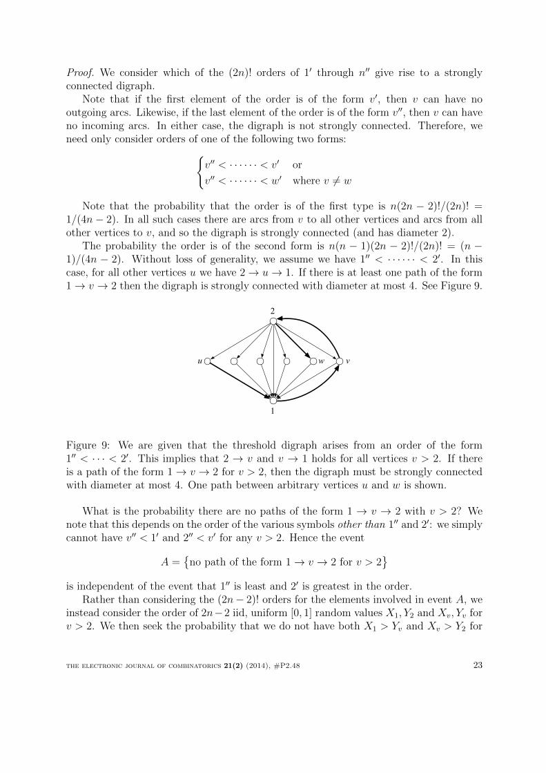
The probability the order is of the second form is n(n − 1)(2n − 2)!/(2n)! = (n −1)/(4n − 2). Without loss of generality, we assume we have 1′′ < · · · · · · < 2′. In thiscase, for all other vertices u we have 2→ u→ 1. If there is at least one path of the form1→ v → 2 then the digraph is strongly connected with diameter at most 4. See Figure 9.

1

2

v u w

Figure 9: We are given that the threshold digraph arises from an order of the form1′′ < · · · < 2′. This implies that 2 → v and v → 1 holds for all vertices v > 2. If thereis a path of the form 1→ v → 2 for v > 2, then the digraph must be strongly connectedwith diameter at most 4. One path between arbitrary vertices u and w is shown.

What is the probability there are no paths of the form 1 → v → 2 with v > 2? Wenote that this depends on the order of the various symbols other than 1′′ and 2′: we simplycannot have v′′ < 1′ and 2′′ < v′ for any v > 2. Hence the event

A ={

no path of the form 1→ v → 2 for v > 2}

is independent of the event that 1′′ is least and 2′ is greatest in the order.Rather than considering the (2n− 2)! orders for the elements involved in event A, we

instead consider the order of 2n−2 iid, uniform [0, 1] random values X1, Y2 and Xv, Yv forv > 2. We then seek the probability that we do not have both X1 > Yv and Xv > Y2 for


any v > 2. Conditioning on X1 = x and Y2 = y, the probability that x > Yv and Xv > yis x(1− y). Hence

Pr(A) =

∫ 1

0

∫ 1

0

[1− x(1− y)

]n−2dx dy

which evaluates to Hn−1/(n− 1) and the result follows.

Corollary 31.

limn→∞

Pr [Dn is strongly connected] =1

4.

Our analysis shows that, with high probability, if Dn is strongly connected, then itsdiameter is at most 4. Conceivably, a stronger result (lower diameter) may be achievable.However, computer experiments suggest that when Dn is connected, its diameter is either3 or 4. (Ruling out diameter 1 is easy.) These computer experiments lead us to posit thefollowing.

Conjecture 32. For a positive integer k we have

limn→∞

Pr[diam(Dn) = k

∣∣Dn is strongly connected]

=

3/4 for k = 3,

1/4 for k = 4, and

0 otherwise.

In the theory of Erdos-Renyi random graphs, connectivity and Hamiltonicity areclosely linked. It is reasonable to ask: What is the probability that Dn has a directedHamiltonian cycle. And a reasonable guess is: 1

4(the same as the probability of strong

connectivity). However, [11] shows that the probability that a random Ferrers digraphhas a directed Hamiltonian cycle tends to 0 as n→∞. Therefore, with high probabilityDn does not have a directed Hamiltonian cycle. See [11] for details.

4.4 Chromatic number

In this section we show that the chromatic number of Dn is, with high probability, asymp-totically n/2. The definition of the chromatic number of a digraph is the same as for simplegraphs; that is, χ(D) = χ[simp(D)].

Our method is in two steps.First, we show that the clique number of simp(Dn) is, with high probability, asymptot-

ically n/2. We use the same ideas to show that the independence number is asymptoticallyn/4.

Second, we show that the underlying simple graphs of threshold digraphs are perfect.It is known (and easy to prove) that threshold graphs are perfect, so one might hope thatthe underlying simple graph of a threshold digraph is a threshold graph, but that is notthe case. Here’s an example. Let D be the digraph with vertex set [4] and directed edges1→ 2← 3→ 4. Note that D is a threshold digraph and here is a representation:


v 1 2 3 4

f(v) 0.4 0.4 0.7 0.1g(v) 0.2 0.8 0.5 0.5

Note that even though D is a threshold digraph, simp(D) is not a threshold graph.

We begin with the following result concerning the clique number of the underlyingsimple graph of a random threshold digraph. Note that we use CL(·) to denote the sizeof a largest clique in a graph and use ω(1) to denote a function of n that tends to infinityas n→∞.

Proposition 33. With high probability CL[simp(Dn)] ∼ n/2. Specifically, with highprobability we have

n

2− ω(1)

√n 6 CL [simp(Dn)] 6

n

2+ ω(1)

√n.

Proof. Create a random order L of 1′, 1′′, . . . , n′, n′′ and let Dn = T (L). Let G =simp(Dn).

Partition V (Dn) = V (G) = [n] as follows:

A = {v : v′ > v′′} and B = {v : v′ < v′′}.

Note that |A| is a binomial (n, 12) random variable and so

n

2− ω(1)

√n < |A| < n

2+ ω(1)

√n

with high probability.Note that CL(G[A]) 6 CL(G) 6 CL(G[A]) + CL(G[B]).We claim that A is a clique. Let v, w ∈ A. Without loss of generality v′ < w′. It

follows that w′ > v′ > v′′ and so w → v in Dn, ergo w ∼ v in G. Therefore

CL(G) > CL(G[A]) = |A| > n

2− ω(1)

√n.

For the upper bound, it is enough to show that CL(G[B]) = O(√n) with high proba-

bility.Let K be a k-element subset of B; say K = {v1, v2, . . . , vk} and let XK be the indicator

random variable that K is a clique in G[B]. This requires that v′i < v′′i for all i ∈ K(because K ⊆ B). We also claim that no v′i (or v′′i ) can lie between v′j and v′′j in the order.That is, neither of these is possible:

v′j < v′i < v′′j or v′j < v′′i < v′′j . (7)

Here’s why:In the first case, because v′i < v′′j we have vi 6→ vj. But then because v′′i > v′i we have

v′′i > v′j which implies that vj 6→ vi. Therefore vi 6∼ vj contradicting that K is a clique.


In the second case, because v′′i > v′j we have vj 6→ vi. And because v′′j > v′′i > v′i wehave vi 6→ vj. Therefore vi 6∼ vj contradicting that K is a clique.

It follows from (7) that the symbols v′1, v′′1 , v′2, v′′2 , . . . , v

′k, v′′k must be arranged like this:

v′i1 < v′′i1 < v′i2 < v′′i2 < · · · < v′ik < v′′ik .

The probability this happens—and this gives E(XK)—is k!/(2k)!.Now let X =

∑XK where the sum is over all k-element subsets of B. This gives

Pr(X > 0) 6 E(X) 6

(n

k

)k!

(2k)!6

nk

(2k)!.

Put k = 2√n and apply Stirling’s formula to show that E(X)→ 0 as n→∞.

This implies that, with high probability, CL(G[B]) 6 2√n and the results follows.

Next we examine the independence number α of a random threshold digraph.

Proposition 34. With high probability, the independence number of Dn is asymptotic ton/4. Specifically, with high probability we have

n

4− ω(1)

√n 6 α (Dn) 6

n

4+ ω(1)

√n log n.

Proof. In this proof we use the random representation model rather than the randomorder model. Let X1, Y1, . . . , Xn, Yn be iid uniform [0, 1] random variables that producethe random threshold digraph Dn.

First we verify the lower bound. Consider the set I ={v : Xv, Yv <

12

}. Note that

vertices in I form an independent set. The number of vertices in I is a binomial (n, 14)

random variable and so, with high probability, α[Dn] > |I| > n4− ω(1)

√n.

Next we verify the upper bound. Let U = {v : Xv + Yv > 1}. Check that for any twovertices, v, w ∈ U we have v → w or w → v, so a maximum independent set of Dn cancontain at most one vertex in U .

Let L be the complementary set of vertices, {v : Xv + Yv < 1} and let A be a largestindependent subset of L. Note that |A| 6 α[Dn] 6 |A|+ 1.

Among all the vertices in A, choose v with largest X value and w with largest Y value.It may be the case v = w. Let t = Xv.

We claim that Xv + Yw < 1; here’s why. If v = w, then Xv + Yv < 1 because v ∈ L.If v 6= w then Xv + Yw < 1 because A is an independent set.

Therefore Yw < 1−Xv = 1−t. It follows that for any vertex a ∈ A we have Xa 6 t andYa < 1−t. That is, the points representing vertices in A lie in the rectangle [0, t]×[0, 1−t].

For integer k with 1 6 k 6 n, define the rectangle Rk to be

Rk =

[0,k

n

]×[0, 1− k − 1

n

]whose area is less than 1

4+ 1

n. See Figure 10. Note that the rectangle [0, t]× [0, 1− t] is


1n

[0, 1] × [0, 1]

x+

y=

1

R1

R2

R3

Rn

Figure 10: Covering the triangular region {(x, y) ∈ [0, 1]2 : x+ y 6 1} with rectanglesR1, R2, . . . , Rn.

contained an Rk for some k.The expected number of points (Xi, Yi) in an Rk is less than 1

4n+ 1 so the probability

a specific Rk contains more than 14n + 1 + δ points is less than exp {−cδ2/n} for some

absolute constant c > 0. Therefore, the probability any of the Rk contains more than14n + 1 + δ points is bounded by n exp {−cδ2/n}. Taking δ �

√n log n is sufficient to

conclude that, with high probability, α(Dn) 6 n4

+ 2 + δ.

Two comments on this result. First, the extra factor of√

log n in the upper boundis likely just an artifact of our proof technique; we expect it can be eliminated. Second,define a strong clique in a digraph D to be a set of vertices K such that both u → vand v → u for all distinct u, v ∈ K. Then this result implies that the maximum size of astrong clique in Dn is, with high probability, asymptotically n/4 (and we have the samebounds).

We now resume our analysis of the chromatic number of Dn. We know that, with highprobability, CL[simp(Dn)] ∼ n/2; this gives a lower bound on the chromatic number. Infact, the chromatic number equals the clique number.

Recall that a graph G is perfect if χ(H) = CL(H) for all induced subgraphs H of G.Berge [1] conjectured and Chudnovsky, Robertson, Seymour, and Thomas [3] proved thefollowing landmark result.

Theorem 35 (Strong Perfect Graph Theorem). A graph is perfect if and only if it doesnot contain, for any k > 2, an odd hole C2k+1 or an odd antihole C2k+1 as an inducedsubgraph.

We employ this result to show that the underlying simple graph of a threshold digraphis perfect.


Theorem 36. Let D be a threshold digraph and let G = simp(D). Then G is perfect.

We prove this by showing that G does not contain any odd holes or antiholes. Thatfollows once we show that if simp(D) = C2k+1 or simp(D) = C2k+1, then D is not athreshold digraph. A key step in doing this is the following result that characterizes thosethreshold digraphs D such that simp(D) = P4.

Lemma 37. Let D be a threshold digraph and suppose simp(D) = P4 where the verticesare labeled such that we have 1 ∼ 2 ∼ 3 ∼ 4. Then the following conclusions hold:

1. We have both 1→ 2 and 3→ 4, or else we have both 2→ 1 and 4→ 3.

2. We cannot have both 1 → 2 and 4 → 3. Likewise, we cannot have both 2 → 1 and3→ 4.

3. Consequently, we cannot have both 1→ 2 and 2→ 1. Nor can we have both 3→ 4and 4→ 3.

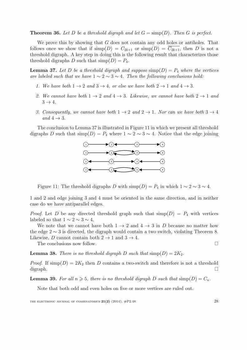
The conclusion to Lemma 37 is illustrated in Figure 11 in which we present all thresholddigraphs D such that simp(D) = P4 where 1 ∼ 2 ∼ 3 ∼ 4. Notice that the edge joining

1 2 3 4

1 2 3 4

1 2 3 4

1 2 3 4

Figure 11: The threshold digraphs D with simp(D) = P4 in which 1 ∼ 2 ∼ 3 ∼ 4.

1 and 2 and edge joining 3 and 4 must be oriented in the same direction, and in neithercase do we have antiparallel edges.

Proof. Let D be any directed threshold graph such that simp(D) = P4 with verticeslabeled so that 1 ∼ 2 ∼ 3 ∼ 4.

We note that we cannot have both 1 → 2 and 4 → 3 in D because no matter howthe edge 2 ∼ 3 is directed, the digraph would contain a two switch, violating Theorem 8.Likewise, D cannot contain both 2→ 1 and 3→ 4.

The conclusions now follow.

Lemma 38. There is no threshold digraph D such that simp(D) = 2K2.

Proof. If simp(D) = 2K2 then D contains a two-switch and therefore is not a thresholddigraph.

Lemma 39. For all n > 5, there is no threshold digraph D such that simp(D) = Cn.

Note that both odd and even holes on five or more vertices are ruled out.


Proof. Let n > 5 and suppose, for contradiction, that D is a threshold digraph withsimp(D) = Cn.

If n > 6, then Cn contains 2K2 as an induced subgraph and this leads to a contradictionof Lemma 38.

It remains to consider the case simp(D) = C5 in which, say, we have 1 ∼ 2 ∼ 3 ∼ 4 ∼5 ∼ 1.

We claim that D does not contain a pair of antiparallel edges. Otherwise, suppose1 → 2 and 2 → 1 in D. Form the digraph D′ by deleting vertex 5 from D. Thensimp(D) = P4 but the antiparallel edges joining vertices 1 and 2 contradicting Lemma 37.

Without loss of generality we have 1→ 2 in D (and not 2→ 1). Considering vertices1, 2, 3, 4, Lemma 37 implies that we must have 3 → 4. Considering vertices 3, 4, 5, 1,Lemma 37 implies that 5 → 1. Considering 5, 1, 2, 3 gives 2 → 3. Considering 2, 3, 4, 5gives 4→ 5. Therefore D is a directed five-cycle consisting exactly of the edges 1→ 2→3→ 4→ 5→ 1 and none of the reverse arcs.

But then 1→ 2 and 3→ 4 form a two-switch.⇒⇐

Next we examine those threshold digraphs D such that simp(D) = C4.

Lemma 40. Let D be a threshold digraph with simp(D) = C4. Then D is isomorphic toa threshold digraph with exactly these edges: 1→ 2← 3→ 4← 1.

Proof. Let D be a threshold digraph with simp(D) = C4 in which 1 ∼ 2 ∼ 3 ∼ 4 ∼ 1.Without loss of generality, 1→ 2 in D (we have not yet ruled out 2→ 1).

The digraph D must contain 3 → 4 or 3 ← 4, but the latter can be ruled out forotherwise D would contain a two-switch. By the same reasoning, D cannot also contain2→ 1 for otherwise 2→ 1 and 3→ 4 would form a two-switch. Thus we have 1→ 2 and3→ 4, but neither reverse arc.

By the same reasoning applied to 2 ∼ 3 and 4 ∼ 1 we have exactly one of (a) 2 → 3and 4 → 1 or (b) 3 → 2 and 1 → 4. However, we can rule out (a) because then 1 → 2and 3→ 4 would form a two-switch.

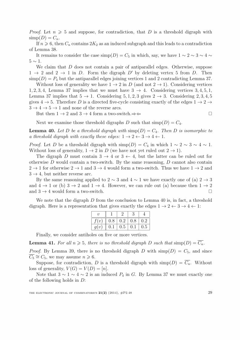
We note that the digraph D from the conclusion to Lemma 40 is, in fact, a thresholddigraph. Here is a representation that gives exactly the edges 1→ 2← 3→ 4← 1:

v 1 2 3 4

f(v) 0.8 0.2 0.8 0.2g(v) 0.1 0.5 0.1 0.5

Finally, we consider antiholes on five or more vertices.

Lemma 41. For all n > 5, there is no threshold digraph D such that simp(D) = Cn.

Proof. By Lemma 39, there is no threshold digraph D with simp(D) = C5, and sinceC5∼= C5, we may assume n > 6.Suppose, for contradiction, D is a threshold digraph with simp(D) = Cn. Without

loss of generality, V (G) = V (D) = [n].Note that 3 ∼ 1 ∼ 4 ∼ 2 is an induced P4 in G. By Lemma 37 we must exactly one

of the following holds in D:


• 1→ 3 and 2→ 4 but 3 6→ 1 and 4 6→ 2, or

• 3→ 1 and 4→ 2 but 1 6→ 3 and 2 6→ 4.

Without loss of generality, we have the former: 1→ 3 and 2→ 4.Next consider vertices {2, 3, 4, 5} and observe that 4 ∼ 2 ∼ 5 ∼ 3 is an induced P4 in

G. Since 2→ 4 in D, we must also have 3→ 5.Likewise, considering vertices {3, 4, 5, 6}, knowing that 3→ 5 in D implies 4→ 6.Continuing in this fashion, in D we have all of the following

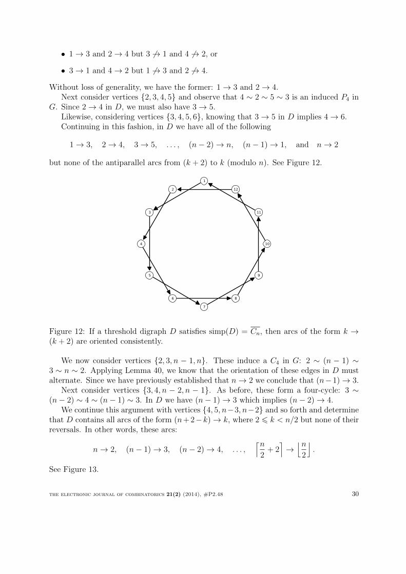
1→ 3, 2→ 4, 3→ 5, . . . , (n− 2)→ n, (n− 1)→ 1, and n→ 2

but none of the antiparallel arcs from (k + 2) to k (modulo n). See Figure 12.

1

2

3

4

5

6

7

8

9

10

11

12

Figure 12: If a threshold digraph D satisfies simp(D) = Cn, then arcs of the form k →(k + 2) are oriented consistently.

We now consider vertices {2, 3, n − 1, n}. These induce a C4 in G: 2 ∼ (n − 1) ∼3 ∼ n ∼ 2. Applying Lemma 40, we know that the orientation of these edges in D mustalternate. Since we have previously established that n→ 2 we conclude that (n−1)→ 3.

Next consider vertices {3, 4, n − 2, n − 1}. As before, these form a four-cycle: 3 ∼(n− 2) ∼ 4 ∼ (n− 1) ∼ 3. In D we have (n− 1)→ 3 which implies (n− 2)→ 4.

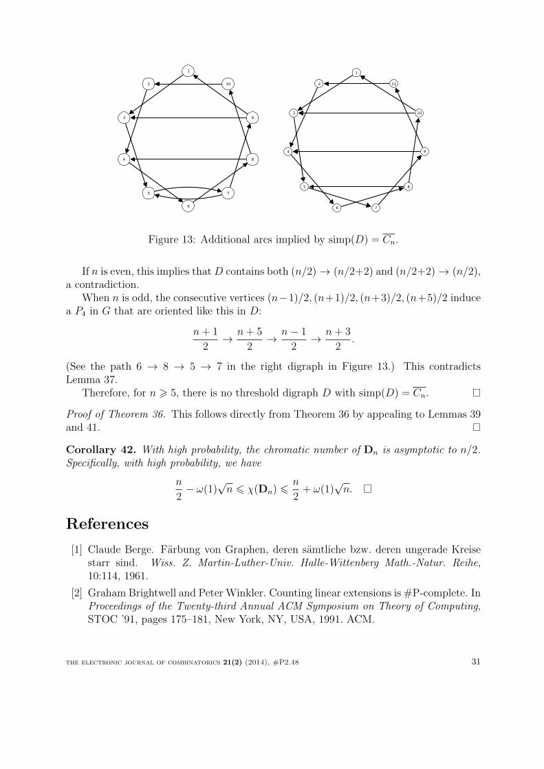
We continue this argument with vertices {4, 5, n−3, n−2} and so forth and determinethat D contains all arcs of the form (n+ 2−k)→ k, where 2 6 k < n/2 but none of theirreversals. In other words, these arcs:

n→ 2, (n− 1)→ 3, (n− 2)→ 4, . . . ,⌈n

2+ 2⌉→⌊n

2

⌋.

See Figure 13.


1

2

3

4

5

6

7

8

9

10

1

2

3

4

5

6 7

8

9

10

11

Figure 13: Additional arcs implied by simp(D) = Cn.

If n is even, this implies that D contains both (n/2)→ (n/2+2) and (n/2+2)→ (n/2),a contradiction.

When n is odd, the consecutive vertices (n−1)/2, (n+1)/2, (n+3)/2, (n+5)/2 inducea P4 in G that are oriented like this in D:

n+ 1

2→ n+ 5

2→ n− 1

2→ n+ 3

2.

(See the path 6 → 8 → 5 → 7 in the right digraph in Figure 13.) This contradictsLemma 37.

Therefore, for n > 5, there is no threshold digraph D with simp(D) = Cn.

Proof of Theorem 36. This follows directly from Theorem 36 by appealing to Lemmas 39and 41.

Corollary 42. With high probability, the chromatic number of Dn is asymptotic to n/2.Specifically, with high probability, we have

n

2− ω(1)

√n 6 χ(Dn) 6

n

2+ ω(1)

√n.

References

[1] Claude Berge. Farbung von Graphen, deren samtliche bzw. deren ungerade Kreisestarr sind. Wiss. Z. Martin-Luther-Univ. Halle-Wittenberg Math.-Natur. Reihe,10:114, 1961.

[2] Graham Brightwell and Peter Winkler. Counting linear extensions is #P-complete. InProceedings of the Twenty-third Annual ACM Symposium on Theory of Computing,STOC ’91, pages 175–181, New York, NY, USA, 1991. ACM.


[3] Maria Chudnovsky, Neil Robertson, Paul Seymour, and Robin Thomas. The strongperfect graph theorem. Annals of Mathematics, 164:51–229, 2006.

[4] V. Chvatal and P.L. Hammer. Aggregation of inequalities in integer programming.In P.L. Hammer, E.L. Johnson, B.H. Korte, and G.L. Nemhauser, editors, Studies inInteger Programming, volume 1 of Annals of Discrete Mathematics, pages 145–162.North-Holland, 1977.

[5] Brian Cloteaux, M. Drew LaMar, Elizabeth Moseman, and James Shook. Thresholddigraphs. Preprint, 2012. arXiv:1212.1149

[6] Olivier Cogis. Ferrers digraphs and threshold graphs. Discrete Mathematics, 38(1):33– 46, 1982.

[7] Persi Diaconis, Susan Holmes, and Svante Janson. Threshold graph limits and ran-dom threshold graphs. Internet Mathematics, 5(3):267–320, 2008.

[8] Martin C. Golumbic. Algorithmic Graph Theory and Perfect Graphs. AcademicPress, 1980.

[9] W. Hoeffding. A class of statistics with asymptotically normal distribution. Annalsof Mathematical Statistics, 19:293–325, 1948.

[10] N.V.R. Mahadev and U.N. Peled. Threshold Graphs and Related Topics. North-Holland, 1995.

[11] Elizabeth Reilly. Random Threshold Graphs and Related Topics. PhD thesis, JohnsHopkins University, 2009.

[12] Elizabeth Reilly and Edward Scheinerman. Random threshold graphs. ElectronicJournal of Combinatorics, 16(1), 2009. R130.

[13] Christopher Ross. Properties of random difference graphs. Electronic Journal ofCombinatorics, 19(4), 2012. P28.

[14] Robert J. Serfling. Approximation Theorems of Mathematical Statistics. Wiley, 1980.

[15] William T. Trotter. Combinatorics and Partially Ordered Sets: Dimension Theory.Johns Hopkins University Press, 1992.

[16] Stephen J. Young and Edward Scheinerman. Directed random dot product graphs.Internet Mathematics, 5(1–2):91–112, 2008.


http://arxiv.org/abs/1212.1149

Documents

Random Threshold Digraphs