Embed Size (px)
Citation preview

Universita degli studi Milano BicoccaFacolta di Scienze Fisiche Matematiche e Naturali
Radiofrequency Design andMeasurements of a Linear HadronAccelerator for Cancer Therapy
Tesi di LAUREA SPECIALISTICA in FISICAindirizzo in Fisica delle Particelle Elementari
Sessione: Settembre 2008
Candidato: Paolo Puggioni
Relatore Interno: Prof. Stefano RagazziRelatore Esterno: Prof. Ugo Amaldi

ii

to Isabella

iv

Abstract
Cancer is the second cause of death in the developed countries. Nowdays two third ofthe patients are treated with conventional radiotherapy alone (X-rays) or in combinationwith other modalities. The aim of radiotherapy is to induce cells death or apoptosis inthe tumoral site with a minimum damage to surrounding organs.
Thanks to the well known Bragg peak, protons have higher conformity in dose deliverywith respect to X-rays. Deep tumoral sites can be treated with protons energies of about200 MeV and the surrounding tissues get less damages.
In 2004 TERA (Fondazione per la Adroterapia Oncologica) completed the design ofIDRA (Institute for Diagnostic and Advanced Radiotherapy), a physical and culturalspace where experts in nuclear physics and protontherapy would find all the facilities towork together with the common aim to diagnose and defeat cancer.
The heart of IDRA is a proton cyclinac: a 30 MeV cyclotron is the injector of a highfrequency compact linear accelerator that boosts protons from 30 up to 230 MeV.
High frequency is needed to achieve compactness and this is the first 3 GHz protonlinac. Moreover cavities at 30 MeV are unusually thin and this forces the designer to con-sider second order corrections that are neglected in standard calculations. The subjectof this thesis is the design of the linac accelerating cavities, performed by using 2D and3D electromagnetic solver codes.
In this work, the detailed study of the physics of coupled cavities brought importantand novel results both theoretically and experimentally.
The first issue is related to the investigation of the effects of the boundary conditionsand symmetry breaking in finite chain structures. The inquiry of finite structures thatpreserve the infinite chain symmetry is the only way to obtain the parameters of aninfinite chain of coupled cavities.
This result is extremely important because many methods normally used in the labo-ratory and proposed in literature are based on structures having the uncorrect symmetryand thus giving inaccurate results.
For the first time, this study explained the effect of the decrease of the π/2 modefrequency with the increasing number of cavities in chains with half accelerating cells ter-minations. The theoretical model reproduces with very high accuracy the experimentaland simulated measurements.
These theoretical studies enabled the development of a precise procedure to obtaincavities parameters with 3D simulations. This method exploits a five cavities chain withhalf coupling cells terminations that preserve the symmetry of the infinite chain.
This innovative analytical method, compared to the previous iterative ones, has therelevant practical implication of being less time consuming and of improving the precision
v

vi
of the results.The application of this rationale made possible the design and the optimization of the
first module of the linac and a study of the mechanical tolerances of its cavities.
To check the accuracy of the manufacturing, cavities parameters need to be carefullymeasured. Therefore a precise experimental method was conceived taking into account allthe considerations made on the symmetries of chain boundaries. New technical solutionswere studied to avoid systematic errors and then tested by comparing measurements andsimulations.
The final topic concerns a preliminary design of the bridge coupler, the item locatedbetween two accelerating tanks that receives the power needed for particle acceleration.The agreement between theoretical calculations and 3D simulations has been demon-strated and now it is possible to minimize the losses due to power reflection.
The final achievement of this work is the completion of the linac design. ADAM(Accelerators and Detectors for Applications in Medicine), a Swiss company which is aspin-off of CERN, is going to start in January 2009 the construction of the first twomodules, which constitute what is called the First Unit.
Currently, the design methods developed in this thesis are been used for the design ofa liner booster adapted to Carbon ions. This accelerator is going to be coupled to a 230MeV/u cycoltron.

Contents
1 Introduction 11.1 Protontherapy . . . . . . . . . . . . . . . . . . . . . . . . . . . . . . . . . 1
1.1.1 Energy loss of heavy charged particles in matter . . . . . . . . . . 21.1.2 Dose delivery techniques . . . . . . . . . . . . . . . . . . . . . . . . 4
1.2 IDRA and LIGHT . . . . . . . . . . . . . . . . . . . . . . . . . . . . . . . 81.2.1 IDRA components . . . . . . . . . . . . . . . . . . . . . . . . . . . 101.2.2 LIGHT . . . . . . . . . . . . . . . . . . . . . . . . . . . . . . . . . 10
1.3 First Unit . . . . . . . . . . . . . . . . . . . . . . . . . . . . . . . . . . . . 111.4 Original work . . . . . . . . . . . . . . . . . . . . . . . . . . . . . . . . . . 11
2 Accelerating protons in LIGHT 152.1 Overview . . . . . . . . . . . . . . . . . . . . . . . . . . . . . . . . . . . . 152.2 RF acceleration in linacs . . . . . . . . . . . . . . . . . . . . . . . . . . . . 17
2.2.1 RF fields types and modes in cavities . . . . . . . . . . . . . . . . 172.2.2 Particle acceleration . . . . . . . . . . . . . . . . . . . . . . . . . . 172.2.3 Figures of merit . . . . . . . . . . . . . . . . . . . . . . . . . . . . 19
2.3 Longitudinal beam dynamics . . . . . . . . . . . . . . . . . . . . . . . . . 212.3.1 Longitudinal beam dynamics in LIGHT . . . . . . . . . . . . . . . 23
3 Detailed theory of coupled cavities 253.1 From Maxwell equations to a shunt-resonant model . . . . . . . . . . . . . 25
3.1.1 One cavity shunt-resonant model . . . . . . . . . . . . . . . . . . . 263.1.2 Coupling coefficients . . . . . . . . . . . . . . . . . . . . . . . . . . 27
3.2 Coupled oscillators . . . . . . . . . . . . . . . . . . . . . . . . . . . . . . . 283.3 LIGHT model . . . . . . . . . . . . . . . . . . . . . . . . . . . . . . . . . . 293.4 Infinite biperiodic chain . . . . . . . . . . . . . . . . . . . . . . . . . . . . 30
3.4.1 Stopband and π/2 mode . . . . . . . . . . . . . . . . . . . . . . . . 313.5 Chain with different first order couplings . . . . . . . . . . . . . . . . . . . 33
4 A new study of symmetry breaking in finite chains 354.1 Different terminations . . . . . . . . . . . . . . . . . . . . . . . . . . . . . 35
4.1.1 Half CC termination (preserved symmetry) . . . . . . . . . . . . . 354.1.2 Half AC termination (preserved symmetry) . . . . . . . . . . . . . 364.1.3 Half AC termination (broken symmetry) . . . . . . . . . . . . . . . 364.1.4 End Cell termination . . . . . . . . . . . . . . . . . . . . . . . . . . 38
4.2 Symmetry effect on ωπ2
in finite chain structures . . . . . . . . . . . . . . 394.2.1 Introduction . . . . . . . . . . . . . . . . . . . . . . . . . . . . . . 394.2.2 Theoretical model . . . . . . . . . . . . . . . . . . . . . . . . . . . 40
vii

viii CONTENTS
4.2.3 Validation of the model . . . . . . . . . . . . . . . . . . . . . . . . 41
5 New methods to calculate cavities parameters 435.1 Simulation codes . . . . . . . . . . . . . . . . . . . . . . . . . . . . . . . . 43
5.1.1 Superfish . . . . . . . . . . . . . . . . . . . . . . . . . . . . . . . . 435.1.2 CST-Microwave Studio . . . . . . . . . . . . . . . . . . . . . . . . 44
5.2 Finding out cavities parameters . . . . . . . . . . . . . . . . . . . . . . . . 445.2.1 Previous method and related problems . . . . . . . . . . . . . . . . 445.2.2 A new analytical method to find out the 5 cavity parameters of an
infinite chain . . . . . . . . . . . . . . . . . . . . . . . . . . . . . . 455.3 End cells . . . . . . . . . . . . . . . . . . . . . . . . . . . . . . . . . . . . . 46
5.3.1 A new analytical method to check the ωe accuracy . . . . . . . . . 475.3.2 Dispersion relation considering EC . . . . . . . . . . . . . . . . . . 49
6 Tank design algorithm and results 536.1 Cell geometry overview . . . . . . . . . . . . . . . . . . . . . . . . . . . . 53
6.1.1 Tuning tools . . . . . . . . . . . . . . . . . . . . . . . . . . . . . . 546.2 Introduction to tank design . . . . . . . . . . . . . . . . . . . . . . . . . . 556.3 Guessing the frequency . . . . . . . . . . . . . . . . . . . . . . . . . . . . . 566.4 Cavity and AC nose design optimization . . . . . . . . . . . . . . . . . . . 566.5 Coupling slot optimization . . . . . . . . . . . . . . . . . . . . . . . . . . . 58
6.5.1 Effects of the coupling value k1 . . . . . . . . . . . . . . . . . . . . 586.5.2 Choice of k1 . . . . . . . . . . . . . . . . . . . . . . . . . . . . . . . 606.5.3 Oval slot proposal . . . . . . . . . . . . . . . . . . . . . . . . . . . 61
6.6 Target frequency and stopband . . . . . . . . . . . . . . . . . . . . . . . . 616.6.1 Tuning facilities effect . . . . . . . . . . . . . . . . . . . . . . . . . 616.6.2 Choosing the target frequency . . . . . . . . . . . . . . . . . . . . 626.6.3 ωπ/2 and stopband . . . . . . . . . . . . . . . . . . . . . . . . . . . 62
6.7 Parameters of the four Tanks . . . . . . . . . . . . . . . . . . . . . . . . . 636.7.1 Effects of mechanical tolerances . . . . . . . . . . . . . . . . . . . . 66
7 Measurements of the tank parameters 677.1 Measurements and tuning overview . . . . . . . . . . . . . . . . . . . . . . 677.2 Measurements in different configurations . . . . . . . . . . . . . . . . . . . 67
7.2.1 Half CC terminated triplets . . . . . . . . . . . . . . . . . . . . . . 687.2.2 Half AC terminated triplets . . . . . . . . . . . . . . . . . . . . . . 697.2.3 New technical solutions . . . . . . . . . . . . . . . . . . . . . . . . 70
7.3 Validation of 3D simulation accuracy . . . . . . . . . . . . . . . . . . . . . 707.4 Measuring the cavities of the first tank . . . . . . . . . . . . . . . . . . . . 72
7.4.1 Results . . . . . . . . . . . . . . . . . . . . . . . . . . . . . . . . . 727.4.2 Ring correction for AC . . . . . . . . . . . . . . . . . . . . . . . . . 73
8 Bridge coupler 758.1 Introduction . . . . . . . . . . . . . . . . . . . . . . . . . . . . . . . . . . . 75
8.1.1 Functional and mechanical overview . . . . . . . . . . . . . . . . . 758.1.2 Working rationale . . . . . . . . . . . . . . . . . . . . . . . . . . . 77
8.2 Draft design . . . . . . . . . . . . . . . . . . . . . . . . . . . . . . . . . . . 778.2.1 Validity limits of the approximation . . . . . . . . . . . . . . . . . 788.2.2 Results . . . . . . . . . . . . . . . . . . . . . . . . . . . . . . . . . 798.2.3 kba−bc with different slot dimensions . . . . . . . . . . . . . . . . . 79

CONTENTS ix
8.3 Power supply insertion . . . . . . . . . . . . . . . . . . . . . . . . . . . . . 808.3.1 WG to cavity coupling model . . . . . . . . . . . . . . . . . . . . . 808.3.2 Calculating Qext by CST-Microwave simulations . . . . . . . . . . 828.3.3 Calculating Qext with the draft BC design . . . . . . . . . . . . . . 858.3.4 Extrapolating Qext for the whole tank . . . . . . . . . . . . . . . . 888.3.5 Validity test of the 3D simulation . . . . . . . . . . . . . . . . . . . 88
8.4 Final design procedure . . . . . . . . . . . . . . . . . . . . . . . . . . . . . 92
9 Conclusions 959.1 Achievements . . . . . . . . . . . . . . . . . . . . . . . . . . . . . . . . . . 959.2 Further studies . . . . . . . . . . . . . . . . . . . . . . . . . . . . . . . . . 96
A CST-MICROWAVE mesh and precision tips 97
B Technical guide: measuring tank parameters 99B.1 Measure A – half AC ends . . . . . . . . . . . . . . . . . . . . . . . . . . . 101B.2 Measure B – half CC ends . . . . . . . . . . . . . . . . . . . . . . . . . . . 102B.3 Results . . . . . . . . . . . . . . . . . . . . . . . . . . . . . . . . . . . . . . 107B.4 Reverse the order of the plates 1 and 2 . . . . . . . . . . . . . . . . . . . . 108B.5 Excel Worksheet . . . . . . . . . . . . . . . . . . . . . . . . . . . . . . . . 109
C Scattering matrix 111

x CONTENTS

Chapter 1
Introduction
1.1 Protontherapy
Cancer is the second major cause of death (after cardiovascular diseases) in the developedcountries. About one European citizen over three will have to deal with a cancer episodeduring his/her life [1]. There are about 110 of different types of cancer. This makes verydifficult the development of systemic treatments, like gene and immunotherapy or drugtargetting: despite the efforts of many scientists all over the world, the progress is slowand probably the full success will require few decades.
At present, while waiting for the breakthrough of these methods, the therapeuticapproaches are focused on the local control of the tumoral site before the spreading ofmetastases. Actually about the 50% of tumors are cured with a combination of surgicaland radiotherapy treatments, accompanied by chemotherapy to prevent metastases [46][4].
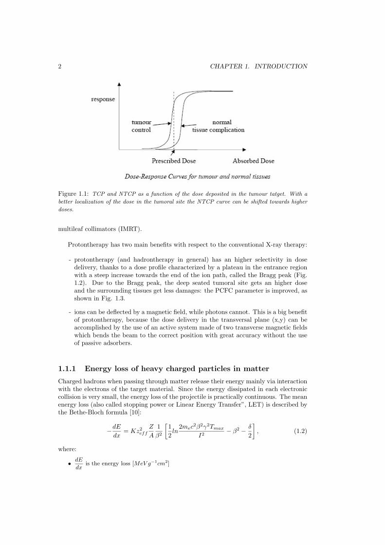
The aim of radiotherapy [5] is to get, for a given dose to the tumour target, thelargest Tumor Control Probability (TCP), keeping at the same time the Normal TissueComplication Probability (NTCP) as low as possible (Fig. 1.1) [54]. An index of efficiencyof the treatment is the Probability for Complication-Free Cure (PCFC) which is given by
PCFC = TCP (1−NTCP ) (1.1)
To improve PCFC, radiations have to destroy all cancer cells in the tumoral site (witha probability that has to be of the order of 10−10!) without damaging surrounding criticalorgans.
Conventional X-ray radiotherapy is performed with electron accelerators: monochro-matic electrons of 5−20 MeV are sent on a heavy target and produce X-ray by Bremsstrahl-ung effect. The dose profile delivered in the tissue reaches a maximum1 after some cmand then has an exponential decrease [2]. It is evident that this profile (in Fig. 1.2) isnot optimal for deep seated tumors because almost all the dose is delivered before thetumoral site, shifting the NTCP curve towards lower doses. The result is improved byradiating the patient from more sides and by modulating the dose delivered in a par-ticular volume by changing the radiation time with the insertion of computer controlled
1As a rule of thumb the depth with the maximum dose delivery RM is found through the followingrelation: RM [cm] = Eγ [MeV ]/6
1
2 CHAPTER 1. INTRODUCTION
Figure 1.1: TCP and NTCP as a function of the dose deposited in the tumour tatget. With a
better localization of the dose in the tumoral site the NTCP curve can be shifted towards higher
doses.
multileaf collimators (IMRT).
Protontherapy has two main benefits with respect to the conventional X-ray therapy:
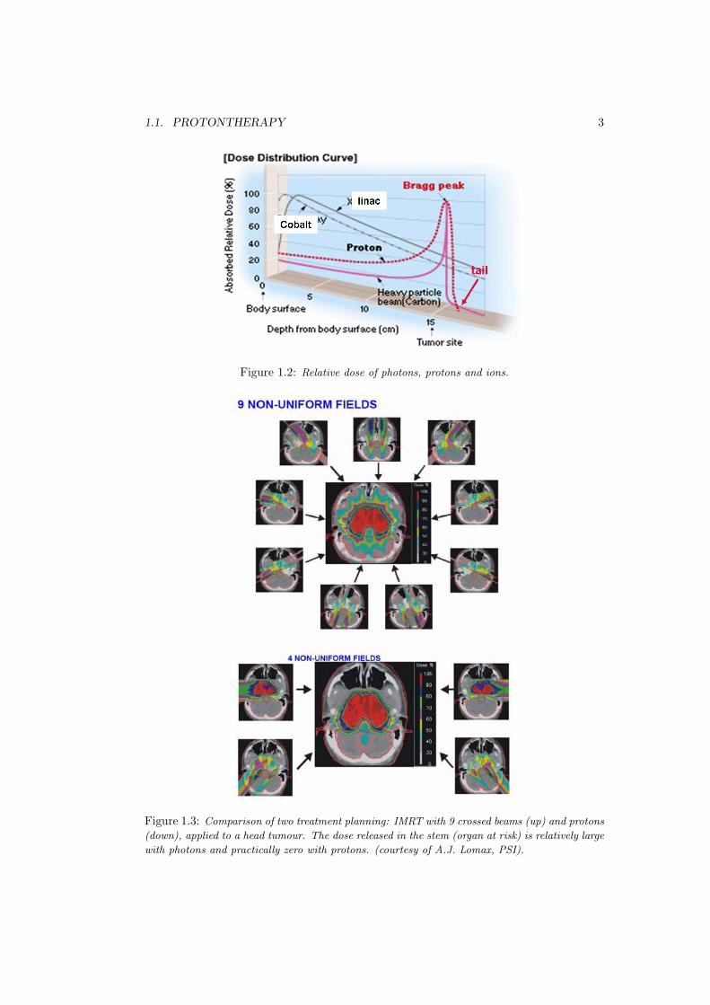
- protontherapy (and hadrontherapy in general) has an higher selectivity in dosedelivery, thanks to a dose profile characterized by a plateau in the entrance regionwith a steep increase towards the end of the ion path, called the Bragg peak (Fig.1.2). Due to the Bragg peak, the deep seated tumoral site gets an higher doseand the surrounding tissues get less damages: the PCFC parameter is improved, asshown in Fig. 1.3.
- ions can be deflected by a magnetic field, while photons cannot. This is a big benefitof protontherapy, because the dose delivery in the transversal plane (x,y) can beaccomplished by the use of an active system made of two transverse magnetic fieldswhich bends the beam to the correct position with great accuracy without the useof passive adsorbers.
1.1.1 Energy loss of heavy charged particles in matter
Charged hadrons when passing through matter release their energy mainly via interactionwith the electrons of the target material. Since the energy dissipated in each electroniccollision is very small, the energy loss of the projectile is practically continuous. The meanenergy loss (also called stopping power or Linear Energy Transfer”, LET) is described bythe Bethe-Bloch formula [10]:
−dE
dx= Kz2
eff
Z
A
1β2
[12ln
2mec2β2γ2Tmax
I2− β2 − δ
2
], (1.2)
where:
• dE
dxis the energy loss [MeV g−1cm2]
1.1. PROTONTHERAPY 3
Figure 1.2: Relative dose of photons, protons and ions.
Figure 1.3: Comparison of two treatment planning: IMRT with 9 crossed beams (up) and protons
(down), applied to a head tumour. The dose released in the stem (organ at risk) is relatively large
with photons and practically zero with protons. (courtesy of A.J. Lomax, PSI).

4 CHAPTER 1. INTRODUCTION
Figure 1.4: Control rates for two head and neck tumour with conventional RT and protontherapy.
• β is the ratio between the particle velocity and the velocity of light c
• zeff is the effective charge of the incident particle
• A is the atomic mass of the medium [g mol−1]
• Z is the atomic number of the medium
• K/A is equal to 4πNAr2emec
2/A whose value is 0.307075 MeV g−1cm2
• I is the mean ionization potential of the atoms of the medium [eV ]
• Tmax is the maximum kinetic energy transfered to a free electron in a single collision
• δ is the density correction to the ionization energy loss.
Since the trajectory is practically straight, the range can be computed by integrating theinverse of the stopping power from the initial energy of the projectile down to zero:
R =∫
E0
0
(dE
dx)−1dE. (1.3)
The beam extracted from the accelerator must have the right energy to match the depthof the tumor.
By manipulating equations 1.2 and 1.3 expressions that describe the relations range-energy and range-LET (which presents the Bragg peak) are found [2]. The prominentBragg peak is due to the β2 appearing in the denominator of Eq. 1.2.
1.1.2 Dose delivery techniques
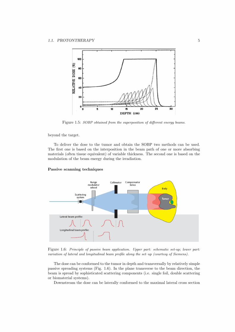
The dose is delivered to the tumor by superimposing many narrow Bragg peaks of dif-ferent energies and therefore different ranges. Their sum results in a Spread-Out BraggPeak (SOBP), as shown in Fig. 1.5. The energy spread in the distal region has to besmaller than 0.5%, in order to have a rapid fall off and spare the normal tissues lying
1.1. PROTONTHERAPY 5
Figure 1.5: SOBP obtained from the superposition of different energy beams.
beyond the target.
To deliver the dose to the tumor and obtain the SOBP two methods can be used.The first one is based on the interposition in the beam path of one or more absorbingmaterials (often tissue equivalent) of variable thickness. The second one is based on themodulation of the beam energy during the irradiation.
Passive scanning techniques
Figure 1.6: Principle of passive beam application. Upper part: schematic set-up; lower part:
variation of lateral and longitudinal beam profile along the set–up (courtesy of Siemens).
The dose can be conformed to the tumor in depth and transversally by relatively simplepassive spreading systems (Fig. 1.6). In the plane transverse to the beam direction, thebeam is spread by sophisticated scattering components (i.e. single foil, double scatteringor biomaterial systems).
Downstream the dose can be laterally conformed to the maximal lateral cross section
6 CHAPTER 1. INTRODUCTION
of the target volume by using specific collimators, made of heavy material. The depthin matter is instead modulated by a rotating absorber or by varying the energy of theaccelerated beam. Since the width of the SOBP is fixed, the dose is conformed only tothe distal edge of the tumor by means of a compensator bolus typically made of tissueequivalent material. This method requires the construction of specific bolus for eachtreatment and, moreover implies non negligible dose to the tissues located upstream ofthe target, as shown in the figure.
Passive beam shaping makes only moderate demands on accelerator, control systemsand electronics. Drawbacks are the limited proximal volume conformity, the demands ofpatient and beam specific devices and the non-conformity of the dose described above.In addition, the large amount of material in the beam path leads to a significant beamenergy and intensity losses, requiring a higher accelerator performance and increasing theneutron and fragment contamination of the beam.
By using continuous magnetic deflection (wobbling) the beam can be laterally spread,with a consequent reduction of the amount of material in the beam path and a better useof the particle fluxes. These wobbling systems are characterized by a fixed beam scan-ning pattern without any feedback between the particle deposition and the beam position.
Active scanning techniques
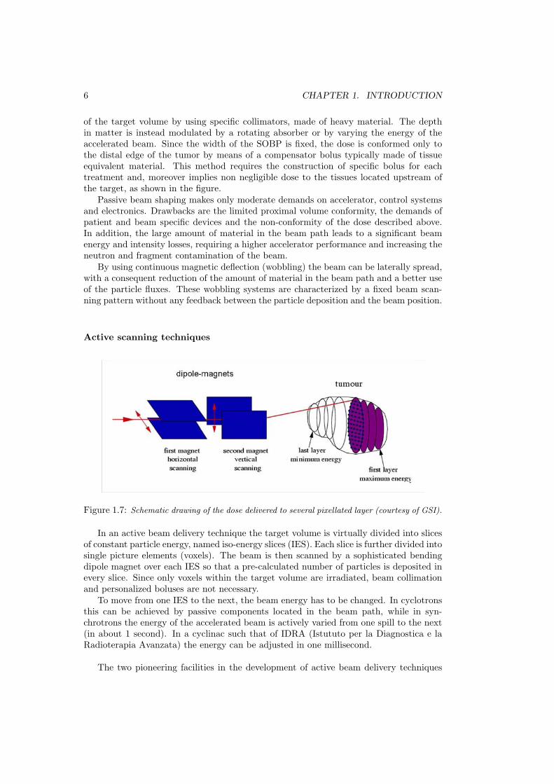
Figure 1.7: Schematic drawing of the dose delivered to several pixellated layer (courtesy of GSI).
In an active beam delivery technique the target volume is virtually divided into slicesof constant particle energy, named iso-energy slices (IES). Each slice is further divided intosingle picture elements (voxels). The beam is then scanned by a sophisticated bendingdipole magnet over each IES so that a pre-calculated number of particles is deposited inevery slice. Since only voxels within the target volume are irradiated, beam collimationand personalized boluses are not necessary.
To move from one IES to the next, the beam energy has to be changed. In cyclotronsthis can be achieved by passive components located in the beam path, while in syn-chrotrons the energy of the accelerated beam is actively varied from one spill to the next(in about 1 second). In a cyclinac such that of IDRA (Istututo per la Diagnostica e laRadioterapia Avanzata) the energy can be adjusted in one millisecond.
The two pioneering facilities in the development of active beam delivery techniques

1.1. PROTONTHERAPY 7
were the Paul Scherrer Institute (PSI, Switzerland) and the Heavy Ion Research Centre(Gesellschaft fur Schwerionenforschung, GSI, Germany).
In 1997 at PSI the first rotating gantry with a 250 MeV proton beam came into oper-ation. Here an active spreading system has been implemented, named “spot scanning”.The dose is deposited in contiguous spots: their centers are separated by 3/4 of their fullwidth at half maximum (FWHM). A transverse dimension and the longitudinal dimensionare covered by acting on a deflecting magnet and an absorber of variable width placedin front of the patient. The thirdlateral dimension is covered by moving the patient bed.The displacement of the spot position is performed with the beam switched off, with atime hole of 5 ms produced by a switch located in the proton extraction line from thecyclotron. The beam is parallel, with a FWHM of about 7 mm, and is scanned in anorthogonal matrix in steps of 4 or 5 mm. For a one liter target volume typically 10000spots are deposited in less than 5 minutes.
In the same year, a different active spreading system named “raster scanning” was putin operation at GSI. The target volume is divided in 10000-30000 voxels, which are treatedin 2-5 minutes. A pencil like beam of 4-10 mm FWHM is moved almost continuouslyby two bending magnets in a preselected pattern over the target area (as does the beamof a TV set), and the desired fluence is delivered to each voxel. To obtain a variablespeed, the beam in moved in steps much smaller (1/3) than the FWHM of the spot. Thenext step is triggered when a predetermined fluence has been recorded by the ionizationchambers placed upstream the patient. In this approach the beam is always on. The GSIsystem takes full advantage of the active energy variation in the synchrotron and scansthe third dimension by changing the energy of the extracted beam from one spill to thenext.
Moving organs
In spot and raster scanning the tumor is painted only once and this is an inconvenient inthe case of moving organs, since any movement can cause important local under-dosagesor over-dosages. Three strategies have been considered to reduce such effects. In orderof increasing complications they are:
1. in the irradiation of the thorax and of the abdominal region the dose delivery is syn-chronized with the patient expiration phase so that the effects of organ movementsare reduced to a minimum;
2. the tumor is painted many times in three dimensions so that organ movements (ifnot too large) can cause only small (≤3%) over-dosages and/or under-dosages (GSIapproach);
3. the movement is detected by a suitable system, which outputs in real-time the 3Dposition of the tumor, and a set of feedback loops compensate for the predicted posi-tion of the dose delivery with on-line adjustments of the transverse and longitudinallocations of the next spots (PSI approach).
The best beam production mechanism is the one that, being fast, allows the use of anycombination of these three approaches: respiratory gating, multi-painting and active en-ergy/angular feedbacks. From this point of view a cyclinac is better than a cyclotron ora synchrotron.
8 CHAPTER 1. INTRODUCTION
1.2 IDRA and LIGHT
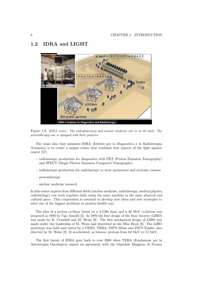
Figure 1.8: IDRA center. The radiopharmacy and nuclear medicine site is on the back. The
protontherapy one is equipped with three gantries.
The main idea that animates IDRA (Istituto per la Diagnostica e la RadioterapiaAvanzata) is to create a unique center that combines four aspects of the fight againstcancer [57]:
- radioisotope production for diagnostics with PET (Proton Emission Tomography)and SPECT (Single Photon Emission Computed Tomography)
- radioisotope production for endotherapy to treat metastases and systemic tumors
- protontherapy
- nuclear medicine research
In this center experts from different fields (nuclear medicine, radiotherapy, medical physics,radiobiology) can work together daily using the same machine in the same physical andcultural space. This cooperation is essential to develop new ideas and new strategies tosolve one of the biggest problems in modern health care.
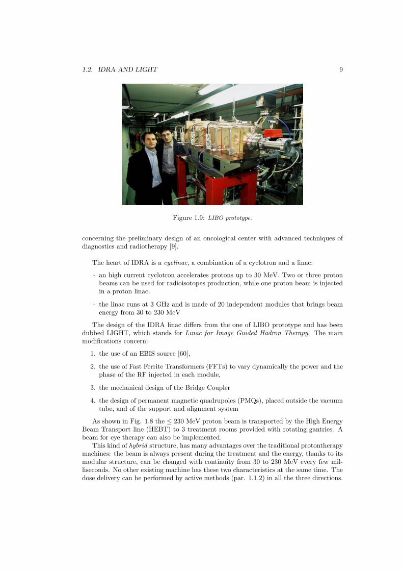
The idea of a proton cyclinac based on a 3 GHz linac and a 30 MeV cyclotron wasproposed in 1993 by Ugo Amaldi [3]. In 1994 the first design of the linac booster (LIBO)was made by K. Crandall and M. Weiss [9]. The first mechanical design of LIBO wasmade under the leadership of M. Weiss and described in the Blue Book [6]. The LIBOprototype was built and tested by a CERN, TERA, INFN-Milan and INFN-Naples, alsodirected by M. Weiss [8]. It accelerated, as forseen, protons from 62 MeV to 74 MeV.
The first layout of IDRA goes back to year 2000 when TERA (Fondazione per laAdroterapia Oncologica) signed an agreement with the Ospedale Maggiore di Novara
1.2. IDRA AND LIGHT 9
Figure 1.9: LIBO prototype.
concerning the preliminary design of an oncological center with advanced techniques ofdiagnostics and radiotherapy [9].
The heart of IDRA is a cyclinac, a combination of a cyclotron and a linac:
- an high current cyclotron accelerates protons up to 30 MeV. Two or three protonbeams can be used for radioisotopes production, while one proton beam is injectedin a proton linac.
- the linac runs at 3 GHz and is made of 20 independent modules that brings beamenergy from 30 to 230 MeV
The design of the IDRA linac differs from the one of LIBO prototype and has beendubbed LIGHT, which stands for Linac for Image Guided Hadron Therapy. The mainmodifications concern:
1. the use of an EBIS source [60],
2. the use of Fast Ferrite Transformers (FFTs) to vary dynamically the power and thephase of the RF injected in each module,
3. the mechanical design of the Bridge Coupler
4. the design of permanent magnetic quadrupoles (PMQs), placed outside the vacuumtube, and of the support and alignment system
As shown in Fig. 1.8 the ≤ 230 MeV proton beam is transported by the High EnergyBeam Transport line (HEBT) to 3 treatment rooms provided with rotating gantries. Abeam for eye therapy can also be implemented.
This kind of hybrid structure, has many advantages over the traditional protontherapymachines: the beam is always present during the treatment and the energy, thanks to itsmodular structure, can be changed with continuity from 30 to 230 MeV every few mil-liseconds. No other existing machine has these two characteristics at the same time. Thedose delivery can be performed by active methods (par. 1.1.2) in all the three directions.

10 CHAPTER 1. INTRODUCTION
1.2.1 IDRA components
The 30 MeV cyclotron from IBA gives a current of 300 µA and consume about 50 kW.The beams have different potential utilisations:
- isotope production, such as 18F, 11C, 15O, 13N for PET and 201Tl, 67Ga, 123I forSPECT.
- generation of thermal or epithermal neutrons beam for Boron Neutron CaptureTherapy (BNCT) and Boron Neutron Capture Synovectomy (BNCS) applications.These applications are still experimental but of great interest for research collabo-rations and universities.
- injection in the linac for protontherapy
Even if the longitudinal acceptance of LIGHT is very small (about 10−4) compared tothe DC nature of the cyclotron beam, the currents needed for therapy are so small (1–2nA) that the original beam of 300 µA is more than sufficient.
1.2.2 LIGHT
LIGHT is a compact 3 GHz proton linear accelerator with an high gradient acceleratingfield. In only 19 m (the dimension of a typical corridor in an hospital) protons areaccelerated from 30 to 230 MeV [7].
LIGHT is made of 10 Units, each of them consists of:
- one klystron of 7.5 MW (peak power) that works at a repetition rate of 200 Hz.
- a RF splitter that split the RF from the klystron into two waveguides that feed twomodules.
- two modules that are fed by the same klystron. The amplitude and the phase ofthe RF peak in each independent module can be adjusted in 1 ms by a Fast FerriteTransformer (FFT).
Figure 1.10: The vertical axis represents the percentage of the maximum number of protons Nm
delivered in each spot. The horizontal axis spans tens of ms and the proton pulses of few µs are
not represented in scale.
As shown in Fig. 1.10, the duty cycle is 0.54× 10⁻³ (pulses of 2.7 µs every 200 Hz).

1.3. FIRST UNIT 11
The time structure of the beam is particularly effective for the spot scanning tech-nique. During the off time (5 ms), the number of protons delivered in the next spotcan be adjusted in a large dynamical range (Nm/50 < N < Nm) by varying the param-eter of the EBIS source used during protontherapy. An accuracy of 3% has been obtained.
1.3 First Unit
As anticipated, between 1998 and 2002 the construction and beam acceleration test ofa prototype of LIBO (with an initial proton energy of 62 MeV) was successfully accom-plished by M. Weiss and collaborators from TERA, CERN, INFN Milano and INFNNapoli [8].
The tests demonstrated for the first time that the matching between a cyclotron anda linac is possible and that a 3 GHz linac structure is capable of accelerating protons.
In 2008 TERA passed all its know–how about cyclinacs to ADAM S.A., a Swisscompany whose aim is to build and test the First Unit of the LIGHT 30–230 MeV beforethe end of 2010 and then to build and test the first IDRA. This Unit will accelerateprotons from 30 to 41.2 MeV in about 1 m with an average electrical field of 13.5 MV/m.
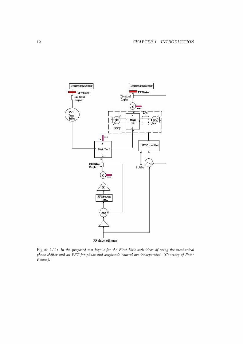
As shown in Fig. 1.11, the First Unit is fed by a single klystron. The power is splitinto two branches by a Magic Tee and each branch feeds one module (Figs. 1.11 and1.12). One branch has a mechanical phase shifter, the other has a FFT for phase andamplitude control. In this way it is possible to test the behavior of both devices.
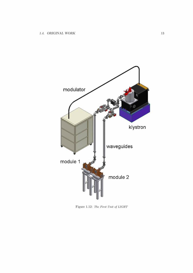
As shown in Fig. 1.12, the power from the waveguides enters the BC through amagnetic coupling. The BC connects the two tanks of the same module. Each tankconsists in 16 accelerating cells (AC) and 15 coupling cells (CC), magnetically coupled ina typical Side Coupled Linac (SCL) structure [56].
In Fig. 8.1, a module of LIGHT is shown in details. Focusing permanent quadrupolemagnets (PMQs) are located under the BC and in the intermodular space.
1.4 Original work
The original work of this thesis consists in:
- the development a new analytical method to achieve a faster and more accuratetank design,
- the optimization of the design of the accelerating cavities (AC) and the couplingcavities (CC) of the tanks,
- the development of a precise method to measure and tune accelerator’s cavities,
- an approximate design of the BC,
- the design of the power matching between the waveguide (WG) and the couplingcavity of the BC.
12 CHAPTER 1. INTRODUCTION
Figure 1.11: In the proposed test layout for the First Unit both ideas of using the mechanical
phase shifter and an FFT for phase and amplitude control are incorporated. (Courtesy of Peter
Pearce).
1.4. ORIGINAL WORK 13
Figure 1.12: The First Unit of LIGHT

14 CHAPTER 1. INTRODUCTION
Chapter 2
Accelerating protons in LIGHT
2.1 Overview
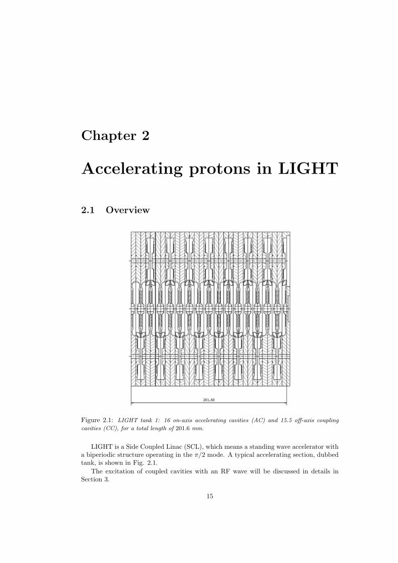
Figure 2.1: LIGHT tank 1: 16 on-axis accelerating cavities (AC) and 15.5 off-axis coupling
cavities (CC), for a total length of 201.6 mm.
LIGHT is a Side Coupled Linac (SCL), which means a standing wave accelerator witha biperiodic structure operating in the π/2 mode. A typical accelerating section, dubbedtank, is shown in Fig. 2.1.
The excitation of coupled cavities with an RF wave will be discussed in details inSection 3.
15

16 CHAPTER 2. ACCELERATING PROTONS IN LIGHT
Figure 2.2: Instantaneous electric field configurations for different structure modes.
In Fig. 2.2 the electric field configurations for different modes are represented. The Efield in π/2 mode follows the scheme [1, 0,−1, 0, . . .] which means that in the first cavityit is directed to the right, in the second it is zero, in the third it is directed to the leftand so on.
Odd cavities (with null field) are named coupling cavities (CC), even cavities arenamed accelerating cavities (AC). On-axis CCs, like the ones in Fig. 2.2, lower the meanaccelerating field because they use space in the longitudinal direction with a null fieldregion. In a SCL, the CCs are shifted off–axis (Fig. 2.1) in order to increase the meanaccelerating field and decrease the length of the tank. In this way ACs come closer toeach other: the drawback is that the coupling between them increases and this effectmust be taken into account (see Sec. 3.3).
The RF fields are reversed every T/2, where T is the period of the RF pulse (T =1/ν = 1/2πω = λ/c). A proton must run from an AC to the next AC in a time T , inorder to find that the electric field has the same direction. The distance d between thecenters of two accelerating cells has thus to be:
d =βλ
2(2.1)
The proton speed increases from AC to AC but it is impossible to change each cell lengthaccordingly: in a tank all cavities have the same length, calculated with a particularalgorithm that finds a mean value β [15].
In the following all parameters influencing the design of the cavities and of the accel-erator as a whole are examined in details.
2.2. RF ACCELERATION IN LINACS 17
2.2 RF acceleration in linacs
2.2.1 RF fields types and modes in cavities
A complete description of the propagation of RF waves in waveguides and cavities isbeyond our purposes and can be found in [29] [17] [48].
In bounded media transverse electromagnetic waves (TEM) are not possible: one ofthe field components must be in the direction of propagation to satisfy boundary con-ditions [24]. If it is an electric component, one has a transverse magnetic (TM) mode;otherwise it is a transverse electric (TE) wave.
In a rectangular waveguide different modes can propagate: TMmn or TEmn. Thesubscripts m and n indicate the number of halfwaves in the x and y direction respectively.
Modes in a cylindrical resonators have three subscripts m, n, p: p indicates the num-ber of halfwaves longitudinally.
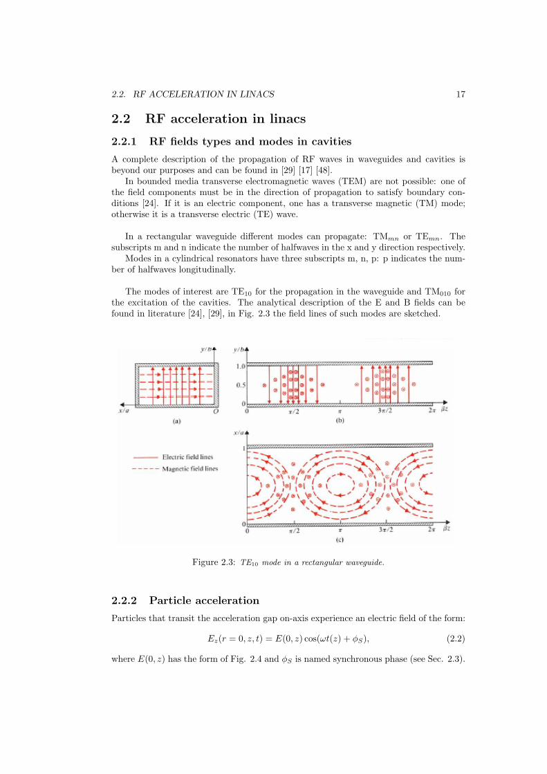
The modes of interest are TE10 for the propagation in the waveguide and TM010 forthe excitation of the cavities. The analytical description of the E and B fields can befound in literature [24], [29], in Fig. 2.3 the field lines of such modes are sketched.
Figure 2.3: TE10 mode in a rectangular waveguide.
2.2.2 Particle acceleration
Particles that transit the acceleration gap on-axis experience an electric field of the form:
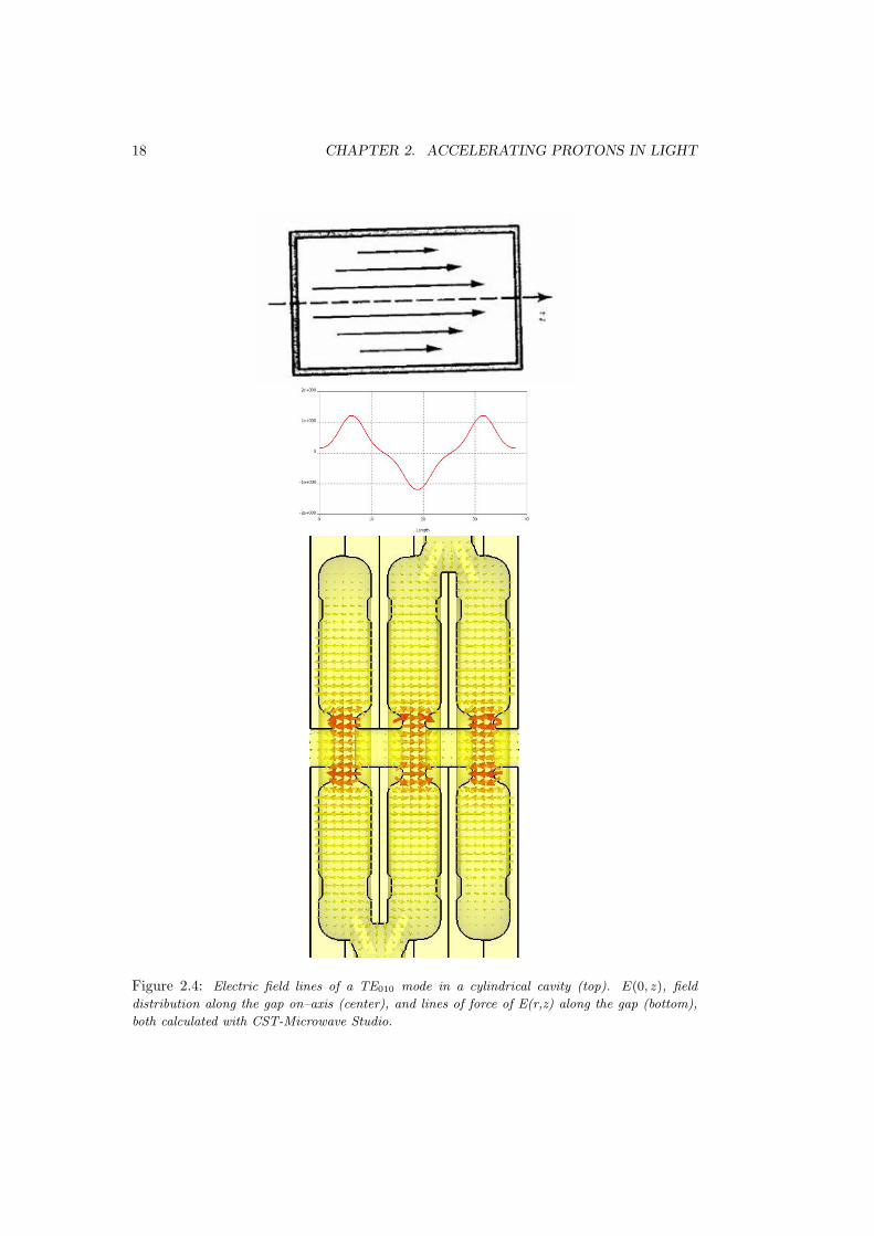
Ez(r = 0, z, t) = E(0, z) cos(ωt(z) + φS), (2.2)
where E(0, z) has the form of Fig. 2.4 and φS is named synchronous phase (see Sec. 2.3).
18 CHAPTER 2. ACCELERATING PROTONS IN LIGHT
Figure 2.4: Electric field lines of a TE010 mode in a cylindrical cavity (top). E(0, z), field
distribution along the gap on–axis (center), and lines of force of E(r,z) along the gap (bottom),
both calculated with CST-Microwave Studio.

2.2. RF ACCELERATION IN LINACS 19
The energy gain ∆W of the particle through a gap of thickness L is simply
∆W = q
∫ L/2
−L/2
E(0, z) cos(ωt(z) + φS)dz (2.3)
that can be written in the following form:
∆W = qV0T sinφS , (2.4)
where V0 is the voltage across the cavity
V0 =∫ L/2
−L/2
E(0, z)dz. (2.5)
T is the the transit time factor
T =
∫ L/2
−L/2E(0, z) cos ωt(z)dz∫ L/2
−L/2E(0, z)dz
(2.6)
which is in the interval [0, 1] and measures the reduction in energy gain caused by thesinusoidal time variation of the field.
In a first approximation [49] T becomes
T =sinπg/βλ
πg/βλ(2.7)
where g is the gap length, and β the speed of the particle. If the gap g is small withrespect to βγ, T approaches 1.
The real beam particles have a position randomly distributed around the beam-axisand they experience an electric field E(r, z) shown in Fig. 2.4 (bottom), different fromthe on–axis field E(0, z). Analytical expressions of E(r, z) are derived and shown in Ref-erence [49]. Beam dynamics programs such as DESIGN [14] and LINAC [15] take intoaccount these corrections.
2.2.3 Figures of merit
The figures of merit that provide informations about the performance of an acceleratingtank are:
- the shunt impedance rs measures the effectiveness of producing an axial voltage V0
for a given power dissipated P ; it is given by:
rs =V 2
0
P. (2.8)
- The shunt impedance per unit of length,
Z =rs
L, (2.9)
where L is the tank length over which the acceleration takes place.
20 CHAPTER 2. ACCELERATING PROTONS IN LIGHT
- The effective shunt impedance per unit of length ZT 2 considers the effective accel-erating voltage is V0T (Eq. 2.4) and it is given by:
ZT 2 =(V0T )2
PL=
(E0T )2
P/L, (2.10)
- The internal quality factor Q0 takes into account the lossy behavior of the resonatordue to the finite conductivity σd of the dielectric of the cavities. It is proportionalto the number of oscillation periods needed to dissipate all the energy stored in thecavity:
Q0 =2πU
TP0=
ωU
P0(2.11)
where ω is the resonant frequency of the cavity, T (in this case) the period ofoscillation, U is the stored energy and P0 is the power dissipated in the cavity.
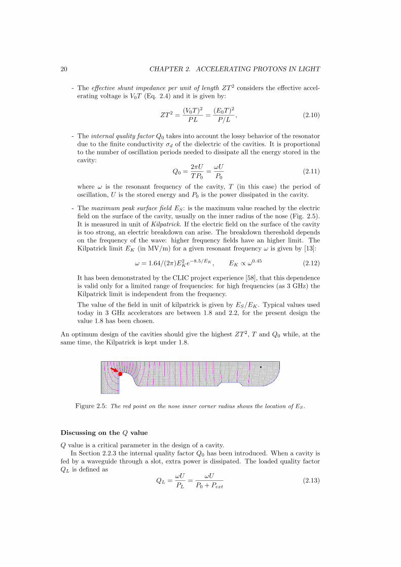
- The maximum peak surface field ES : is the maximum value reached by the electricfield on the surface of the cavity, usually on the inner radius of the nose (Fig. 2.5).It is measured in unit of Kilpatrick. If the electric field on the surface of the cavityis too strong, an electric breakdown can arise. The breakdown thereshold dependson the frequency of the wave: higher frequency fields have an higher limit. TheKilpatrick limit EK (in MV/m) for a given resonant frequency ω is given by [13]:
ω = 1.64/(2π)E2Ke−8.5/EK , EK ∝ ω0.45 (2.12)
It has been demonstrated by the CLIC project experience [58], that this dependenceis valid only for a limited range of frequencies: for high frequencies (as 3 GHz) theKilpatrick limit is independent from the frequency.
The value of the field in unit of kilpatrick is given by ES/EK . Typical values usedtoday in 3 GHz accelerators are between 1.8 and 2.2, for the present design thevalue 1.8 has been chosen.
An optimum design of the cavities should give the highest ZT 2, T and Q0 while, at thesame time, the Kilpatrick is kept under 1.8.
Figure 2.5: The red point on the nose inner corner radius shows the location of ES.
Discussing on the Q value
Q value is a critical parameter in the design of a cavity.In Section 2.2.3 the internal quality factor Q0 has been introduced. When a cavity is
fed by a waveguide through a slot, extra power is dissipated. The loaded quality factorQL is defined as
QL =ωU
PL=
ωU
P0 + Pext(2.13)

2.3. LONGITUDINAL BEAM DYNAMICS 21
where PL is the total power dissipated and Pext is the extra power dissipated due to theslot. Defining the external quality factor Qext with an equation similar to Eq. 2.11, itsatisfies the relation
1QL
=1
Q0+
1Qext
(2.14)
In a free running cavity (when the excitation signal is switched off) the stored energyU varies with time according to
dU(t)dt
= −PL = − ω
QLU (2.15)
and, integrating
U(t) = U0e−t/τw τw =
QL
ω(2.16)
where τw is named filling time.
QL is also related to the width of the resonance peak of a cavity [40]
QL =ω0
∆H(2.17)
where ∆H is the full width at half maximum of the resonance peak and ω0 the resonantfrequency.
2.3 Longitudinal beam dynamics
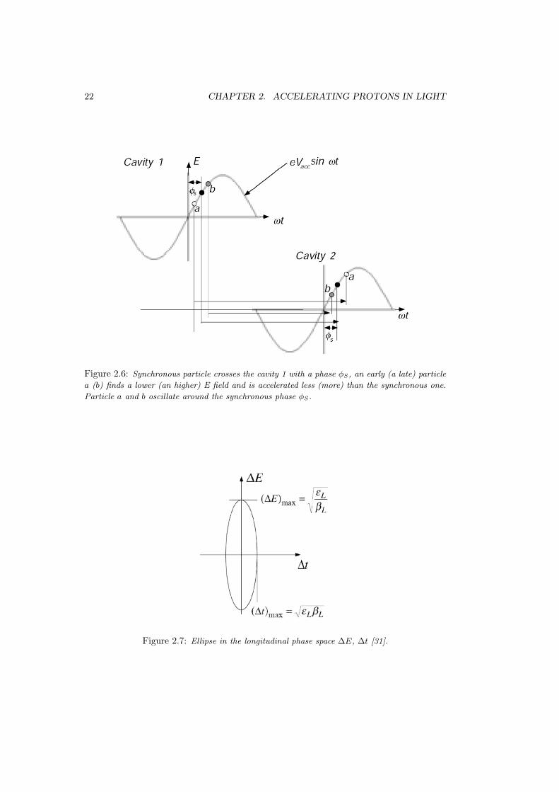
Particles traveling through the accelerator should always cross the mid of the cavities’gaps with the same field phase φS to be accelerated by the same force in each cavity.As explained in Fig. 2.6, particles that cross the cavity with a phase φ 6= φS oscillatearound the synchronous phase φS . These oscillations are considered quantitatively inRefs. [50] [41].
The purpose is to study how ∆E (difference between actual and design energy) is re-lated to φ. The longitudinal motion of the accelerated particles has an invariant quantity:
1βL
(∆t)2 + βL(∆E)2 = εL, (2.18)
where ∆t is the difference between the actual and the synchronous transit time, εL is aconstant named longitudinal emittance and βL (the longitudinal Twiss parameter) is
βL =λ
βSc
√1
2πγ2eV ES cos φS(2.19)
and βS is the speed of the synchronous particle.In order to get a real βL and an effective acceleration, φS must be chosen between
[0, π/2].Eq. 2.18 is represented by an ellipse in the plane ∆E, ∆t (Fig. 2.7) that shows the
maximum variation in energy and time (phase) that can be accepted by the machine.
The equation describing the motion is:
∆E2 + V (φ) = H, (2.20)
22 CHAPTER 2. ACCELERATING PROTONS IN LIGHT
Figure 2.6: Synchronous particle crosses the cavity 1 with a phase φS, an early (a late) particle
a (b) finds a lower (an higher) E field and is accelerated less (more) than the synchronous one.
Particle a and b oscillate around the synchronous phase φS.
Figure 2.7: Ellipse in the longitudinal phase space ∆E, ∆t [31].
2.3. LONGITUDINAL BEAM DYNAMICS 23
whereV (φ) = − 2
(ωβL)2 cos φS(cos φ + φ sinφS) (2.21)
H = − 2(ωβL)2 cos φS
(cos φ0 + φ0 sinφS) (2.22)
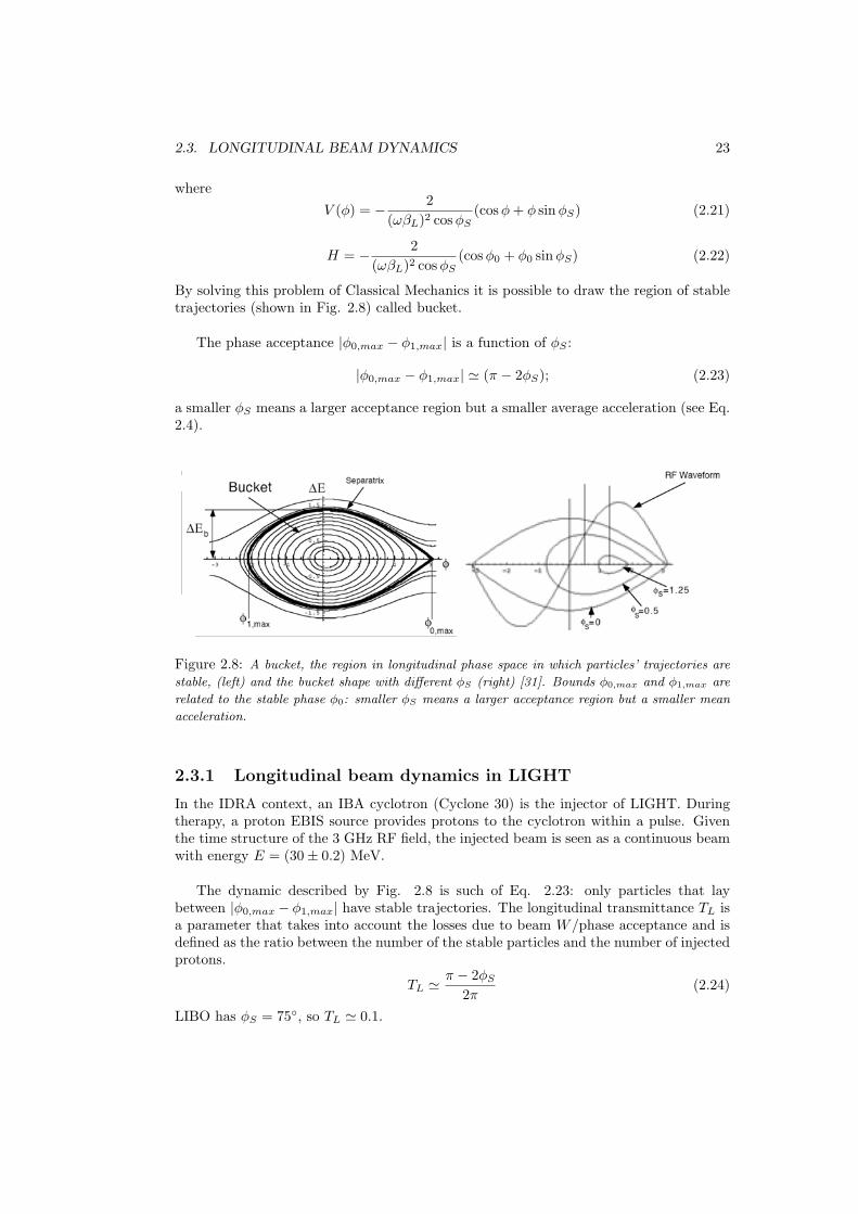
By solving this problem of Classical Mechanics it is possible to draw the region of stabletrajectories (shown in Fig. 2.8) called bucket.
The phase acceptance |φ0,max − φ1,max| is a function of φS :
|φ0,max − φ1,max| ' (π − 2φS); (2.23)
a smaller φS means a larger acceptance region but a smaller average acceleration (see Eq.2.4).
Figure 2.8: A bucket, the region in longitudinal phase space in which particles’ trajectories are
stable, (left) and the bucket shape with different φS (right) [31]. Bounds φ0,max and φ1,max are
related to the stable phase φ0: smaller φS means a larger acceptance region but a smaller mean
acceleration.
2.3.1 Longitudinal beam dynamics in LIGHT
In the IDRA context, an IBA cyclotron (Cyclone 30) is the injector of LIGHT. Duringtherapy, a proton EBIS source provides protons to the cyclotron within a pulse. Giventhe time structure of the 3 GHz RF field, the injected beam is seen as a continuous beamwith energy E = (30± 0.2) MeV.
The dynamic described by Fig. 2.8 is such of Eq. 2.23: only particles that laybetween |φ0,max − φ1,max| have stable trajectories. The longitudinal transmittance TL isa parameter that takes into account the losses due to beam W/phase acceptance and isdefined as the ratio between the number of the stable particles and the number of injectedprotons.
TL 'π − 2φS
2π(2.24)
LIBO has φS = 75, so TL ' 0.1.

24 CHAPTER 2. ACCELERATING PROTONS IN LIGHT
Due to longitudinal transmittance, 90% of protons injected during the RF flat tophave unstable trajectories and hit the accelerating structure. 30-40 MeV protons oncopper can produce radioactive isotopes. Copper activation studies are been carried outto investigate possible problems.
The RF pulses have a repetition rate of 200 Hz with a flat top of 2.7 µs (Fig. 1.10).All protons that are injected out of the power peak are not accelerated and contribute tothe activation problem. To reduce activation, the duration of the proton pulse producedby the EBIS source must be not much longer than 2.7 µs.
Chapter 3
Detailed theory of coupledcavities
3.1 From Maxwell equations to a shunt-resonant model
Maxwell equations describe the propagation of e.m. waves in the cavities of the accelera-tor. An analytical solution of these equations with such complicate boundary conditionsis impossible. Therefore a simplified model is needed.
Solutions of Maxwell equations show that when cavities resonate on a given mode (forexample TM010) the time average energy stored in the electric field equals the averageenergy stored in the magnetic field and that within an RF period the energy oscillatesbetween electric and magnetic [55].
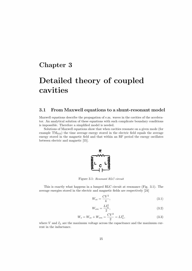
Figure 3.1: Resonant RLC circuit
This is exactly what happens in a lumped RLC circuit at resonance (Fig. 3.1). Theaverage energies stored in the electric and magnetic fields are respectively [24]
Wse =CV 2
4, (3.1)
Wsm =LI2
L
2, (3.2)
Ws = Wse + Wsm =CV 2
2= LI2
L, (3.3)
where V and IL are the maximum voltage across the capacitance and the maximum cur-rent in the inductance.
25

26 CHAPTER 3. DETAILED THEORY OF COUPLED CAVITIES
At resonanceω0 = (2LC)−1/2 (3.4)
V = ω02LIL (3.5)
The power loss is
P =V 2
2R(3.6)
and the quality factor Q is
Q = ω0RC =R
ω02L(3.7)
Thus the parameters of the circuit model R, L, C are directly related to the physicalquantities Q (quality factor), P (power dissipated) and ω0 (resonant frequency) describingthe oscillating cavity.
In the following sections the shunt resonant-circuit model is introduced and its resultsand limits are investigated in detail.
3.1.1 One cavity shunt-resonant model
The fields in an excited cavity can be derived from a vector potential A(r, t) which satisfiesthe wave equation [24]
∇2A(r, t)− 1c2
∂2
∂t2A(r, t) = −µ0J(r, t). (3.8)
A(r, t) can be expanded in terms of a complete set of Eigenmodes
A(r, t) =∑
n
qn(t)An(r), (3.9)
where, for each mode n, An(r, t) = An(r)ejωnt. Performing some calculations [51], qn
must satisfy the following equation
qn +ωn
Qnqn + ω2
nqn =1ε0
∫J(r, t)An(r)dv
A2ndv
(3.10)
with Qn = (ωnUn)/Pn, where Un and Pn are the stored energy and the dissipated energyof the nth mode. This is the equation for a dumped driven oscillator, like the one thatdescribes the RLC circuit of Fig. 3.1
V +ω0V
Q+ ω2
0V =I
C(3.11)
According to this, the physical parameters Q, rs and ω0 have a link to the model pa-rameters R, L and C and an RLC circuit is an effective and simple way to describe anexcited cavity.
3.1. FROM MAXWELL EQUATIONS TO A SHUNT-RESONANT MODEL 27
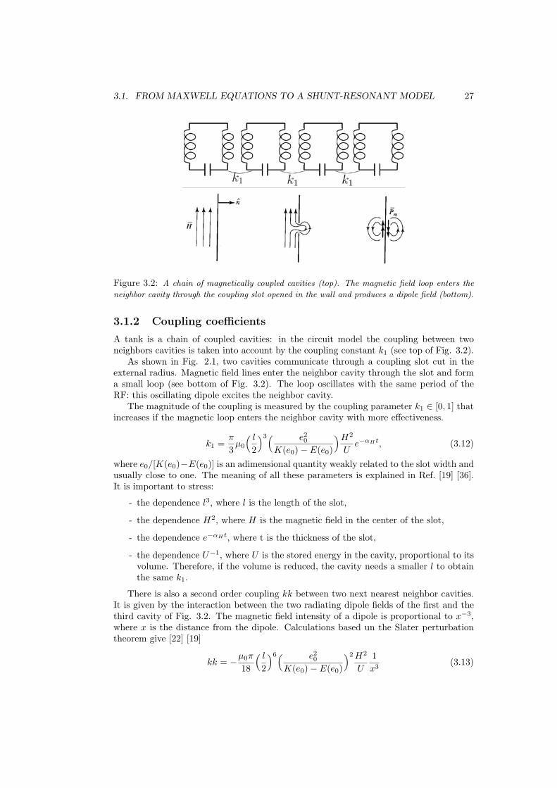
Figure 3.2: A chain of magnetically coupled cavities (top). The magnetic field loop enters the
neighbor cavity through the coupling slot opened in the wall and produces a dipole field (bottom).
3.1.2 Coupling coefficients
A tank is a chain of coupled cavities: in the circuit model the coupling between twoneighbors cavities is taken into account by the coupling constant k1 (see top of Fig. 3.2).
As shown in Fig. 2.1, two cavities communicate through a coupling slot cut in theexternal radius. Magnetic field lines enter the neighbor cavity through the slot and forma small loop (see bottom of Fig. 3.2). The loop oscillates with the same period of theRF: this oscillating dipole excites the neighbor cavity.
The magnitude of the coupling is measured by the coupling parameter k1 ∈ [0, 1] thatincreases if the magnetic loop enters the neighbor cavity with more effectiveness.
k1 =π
3µ0
( l
2
)3( e20
K(e0)− E(e0)
)H2
Ue−αHt, (3.12)
where e0/[K(e0)−E(e0)] is an adimensional quantity weakly related to the slot width andusually close to one. The meaning of all these parameters is explained in Ref. [19] [36].It is important to stress:
- the dependence l3, where l is the length of the slot,
- the dependence H2, where H is the magnetic field in the center of the slot,
- the dependence e−αHt, where t is the thickness of the slot,
- the dependence U−1, where U is the stored energy in the cavity, proportional to itsvolume. Therefore, if the volume is reduced, the cavity needs a smaller l to obtainthe same k1.
There is also a second order coupling kk between two next nearest neighbor cavities.It is given by the interaction between the two radiating dipole fields of the first and thethird cavity of Fig. 3.2. The magnetic field intensity of a dipole is proportional to x−3,where x is the distance from the dipole. Calculations based un the Slater perturbationtheorem give [22] [19]
kk = −µ0π
18
( l
2
)6( e20
K(e0)− E(e0)
)2 H2
U
1x3
(3.13)
28 CHAPTER 3. DETAILED THEORY OF COUPLED CAVITIES
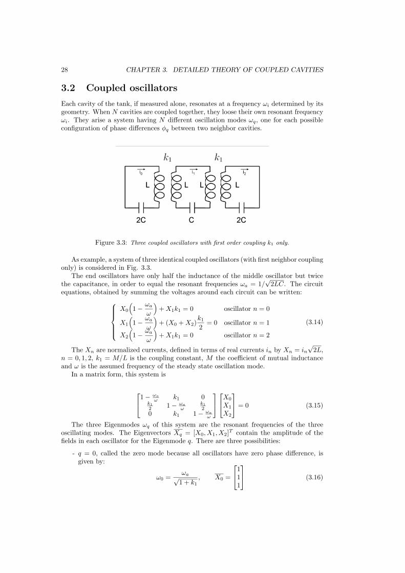
3.2 Coupled oscillators
Each cavity of the tank, if measured alone, resonates at a frequency ωi determined by itsgeometry. When N cavities are coupled together, they loose their own resonant frequencyωi. They arise a system having N different oscillation modes ωq, one for each possibleconfiguration of phase differences φq between two neighbor cavities.
Figure 3.3: Three coupled oscillators with first order coupling k1 only.
As example, a system of three identical coupled oscillators (with first neighbor couplingonly) is considered in Fig. 3.3.
The end oscillators have only half the inductance of the middle oscillator but twicethe capacitance, in order to equal the resonant frequencies ωa = 1/
√2LC. The circuit
equations, obtained by summing the voltages around each circuit can be written:X0
(1− ωa
ω
)+ X1k1 = 0 oscillator n = 0
X1
(1− ωa
ω
)+ (X0 + X2)
k1
2= 0 oscillator n = 1
X2
(1− ωa
ω
)+ X1k1 = 0 oscillator n = 2
(3.14)
The Xn are normalized currents, defined in terms of real currents in by Xn = in√
2L,n = 0, 1, 2, k1 = M/L is the coupling constant, M the coefficient of mutual inductanceand ω is the assumed frequency of the steady state oscillation mode.
In a matrix form, this system is
1− ωa
ω k1 0k12 1− ωa
ωk12
0 k1 1− ωa
ω
X0
X1
X2
= 0 (3.15)
The three Eigenmodes ωq of this system are the resonant frequencies of the threeoscillating modes. The Eigenvectors Xq = [X0, X1, X2]T contain the amplitude of thefields in each oscillator for the Eigenmode q. There are three possibilities:
- q = 0, called the zero mode because all oscillators have zero phase difference, isgiven by:
ω0 =ωa√
1 + k1
, X0 =
111
(3.16)

3.3. LIGHT MODEL 29
- q = 1, called the π/2 mode, is given by:
ω1 = ωa, X1 =
10−1
(3.17)
- q = 2, called the π, is given by:
ω2 =ωa√
1− k1
, X2 =
1−11
(3.18)
These results can be shown on a plot (called dispersion relation) of ωq vs. φ. Since thenumber of modes equals the number of cavities, a long chain has its modes thickened inthe dispersion relation curve. For example, in Fig. 3.4, a dispersion curve for a 7 cavitieschain is shown.
Figure 3.4: Dispersion relation for a chain of 7 coupled oscillators: 7 different modes are excited.
3.3 LIGHT model
LIGHT is the first 3 GHz proton linac accelerator. At 30 MeV it faces an unusuallystrong second order coupling due to the small dimensions of its cavities. The distance dbetween the centers of two accelerating gaps is d = βλ/2 = 12.6 mm (β = 0.25, λ = 10cm). Standard 3 GHz electron linac have cavities 4 times longer (β = 1). 1 GHz protonlinacs have cavities 3 times longer (λ = 30 cm).
Since the second order coupling is proportional to (d−3), it is clear that LIGHT ismuch more affected by this problem than other linacs. Most of the calculations found inliterature do not consider a strong kk, so a more complicate model has been developed.
A LIGHT tank (Fig. 2.1) is a standard SCL biperiodic structure with on-axis ACand off-axis CC. Neighbor CC are set one in the upper and one in the lower semispace inorder to increase their distance and symmetrize the structure.

30 CHAPTER 3. DETAILED THEORY OF COUPLED CAVITIES
A tank can be modeled as a a biperiodic chain of coupled resonators with frequen-cies ωa (AC), ωc (CC) and coupling parameters k1 (AC→CC), ka (AC→AC) and kc
(CC→CC) as shown in Fig. 3.5.
Figure 3.5: An infinite biperiodic chain with first and second neighbor couplings.
All these parameters have to be calculated with very high precision to perform acorrect design of the cavities. Additional problems arise because a tank is not an infinitestructure: the boundary conditions must by adjusted.
Characteristics of an infinite biperiodic chain and boundary conditions are examinedin the following sections.
3.4 Infinite biperiodic chain
Neglecting the effect of the losses, the infinite bipediodic chain of Fig. 3.5 is described bythe set of equations [25] [38] [26]:
V2n = I2n
(2jωLa +
1jωCa
)+ jωk1
√LaLc(I2n+1 + I2n−1) + jωkaLa(I2n+2 + I2n−2)
V2n+1 = I2n+1
(2jωLc +
1jωCc
)+ jωk1
√LaLc(I2n+2 + I2n) + jωkaLa(I2n+3 + I2n−1)
(3.19)where the subscripts a (c) and even (odd) indeces refer to AC (CC).
We set ω2a = 2LaCa, ω2
c = 2LcCc, X2n = I2n
√2La and X2n+1 = I2n+1
√2LC . These
four parameters, related to the LC circuit model, are measurable quantities: the resonantAC and CC frequencies and the square roots of the stored energies in the cavities.
Substituting these relations in the system 3.19:(1− ω2
a
ω2)X2n + k1(X2n+1 + X2n−1) + ka(X2n+2 + X2n−2) = 0
(1− ω2c
ω2)X2n+1 + k1(X2n+2 + X2n) + kc(X2n+3 + X2n−1) = 0
(3.20)
that can be expressed in a matrix form

3.4. INFINITE BIPERIODIC CHAIN 31
. . . . . . . . . . . . . . . . . . . . . . . .
0ka
2k1
2
(1− ωa
ω
) k1
2ka
20 0
0 0kc
2k1
2
(1− ωc
ω
) k1
2kc
20
0 0 0ka
2k1
2
(1− ωa
ω
) k1
2ka
2. . . . . . . . . . . . . . . . . . . . . . . .
. . .
X2n−2
X2n−1
X2n
. . .
= 0 (3.21)
For a finite chain, this system can be solved analytically by finding the Eigenvaluesωq that give the resonant frequencies of the modes q. Each Eigenvalue has an Eigenvec-tor Xq = [. . . , X2n−2, X2n−1, X2n, . . .]T that is related to the strength of E field in thecavities labeled by n.
It is also useful to derive a dispersion relation curve that gives the resonant frequencyfor each mode.
The Eigenvectors of the system 3.20 have the form [25]
X2n = A cos 2nφ X2n+1 = B cos (2n + 1)φ (3.22)
where φ is the oscillation mode
φ =qπ
2Nq = 0, 1, . . . , 2N (3.23)
The index q determines the oscillation mode, while n gives informations about thecavity number and 2N + 1 is the number of cavities (and resonant modes) of a finitechain. For N → ∞, an infinite number of modes is excited and φ becomes a continuousvariable.
By substituting the Xi of 3.22 into the system of equations 3.20, the following systemis obtained:
Bk1 cos φ = −A(1− ω2
a
ω2+ ka cos 2φ
)B
(1− ω2
c
ω2+ kc cos 2φ
)= −Ak1 cos φ
(3.24)
By eliminating A and B and manipulating the expression, the following dispersion relationis found:
k21 cos2 φ =
(1− ω2
a
ω2+ ka cos 2φ
)(1− ω2
c
ω2+ kc cos 2φ
)(3.25)
This equation shows which mode φ is excited at a given frequency ω. The curve ω vs. φis in Fig. 3.6.
3.4.1 Stopband and π/2 mode
The φ = π/2 mode is used in LIGHT because it gives many advantages on performanceand stability:
- frequency errors in the individual cavities do not contribute to amplitude errorsin the whole chain and the sensibility is inversely proportional to the couplingcoefficient k1,
32 CHAPTER 3. DETAILED THEORY OF COUPLED CAVITIES
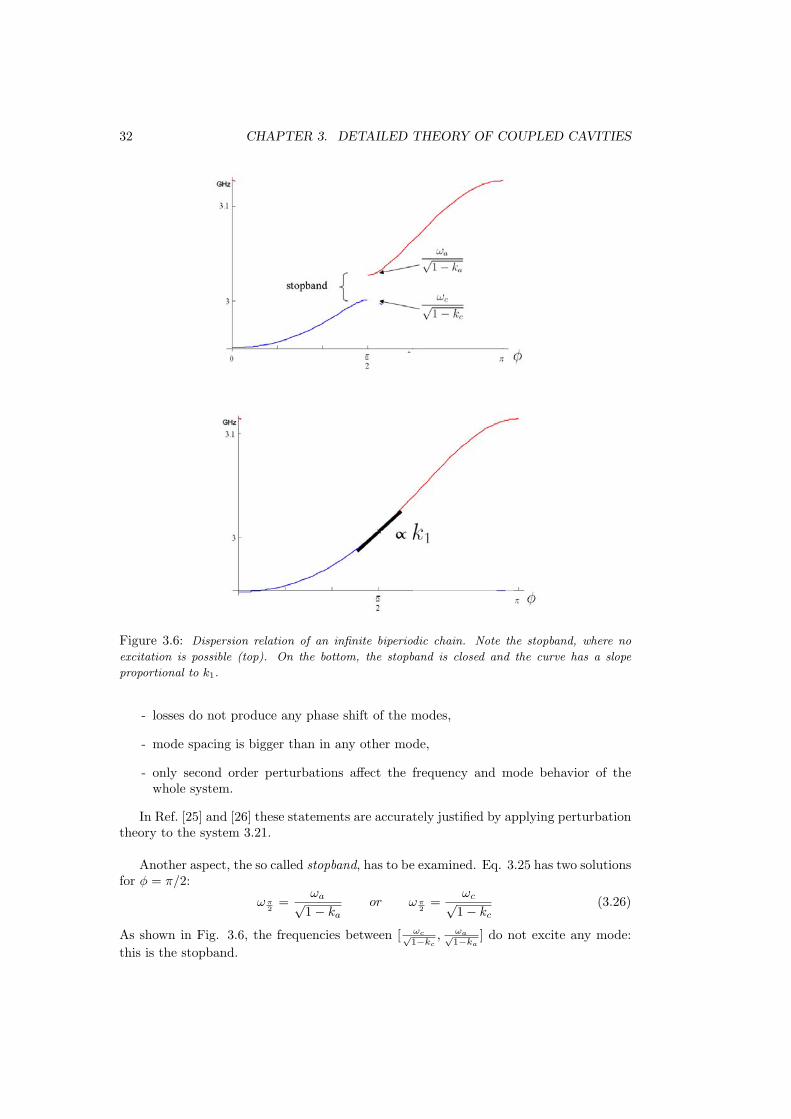
Figure 3.6: Dispersion relation of an infinite biperiodic chain. Note the stopband, where no
excitation is possible (top). On the bottom, the stopband is closed and the curve has a slope
proportional to k1.
- losses do not produce any phase shift of the modes,
- mode spacing is bigger than in any other mode,
- only second order perturbations affect the frequency and mode behavior of thewhole system.
In Ref. [25] and [26] these statements are accurately justified by applying perturbationtheory to the system 3.21.
Another aspect, the so called stopband, has to be examined. Eq. 3.25 has two solutionsfor φ = π/2:
ωπ2
=ωa√
1− ka
or ωπ2
=ωc√
1− kc
(3.26)
As shown in Fig. 3.6, the frequencies between [ ωc√1−kc
, ωa√1−ka
] do not excite any mode:this is the stopband.
3.5. CHAIN WITH DIFFERENT FIRST ORDER COUPLINGS 33
When the stopband is opened the two branches of the dispersion curve approachesπ/2 mode with a zero slope. When the stopband is reduced to zero, by making
ωa/ωc =√
(1− ka)(1− kc), (3.27)
the two branches practically join with a slope proportional to k1 (see Fig. 3.6).Moreover, all advantages of π/2 mode vanish if the stopband is opened. In Ref. [25]
it is proofed that the sensitivity of the system to frequency errors in single cavities isproportional to the amplitude of the stopband.
Therefore it is adviced, to achieve a stable π/2 operating mode, to reduce the stop-band down to 1 MHz (so that a precision better than 1/1000 is required for a 3 GHz linacas LIGHT).
To excite with high precision the π/2 mode, neighbouring modes should be as faraway as possible. This requires that:
- the stopband is closed, in order to have a non-zero slope in the dispersion curve(Fig. 3.6),
- the coupling parameter k1 is large,
- N is kept small because the number of modes is equal to 2N + 1: increasing Nthicken the modes on the dispersion curve shown in Fig. 3.4. For N → ∞, themodes lay on a continuous curve (as in Fig. 3.6) and it is impossible to preciselyexcite the π/2 mode alone.
The spacing δω between the π/2 mode and its neighbors is given by [52]:
δω
ωπ2
= k1π
2N. (3.28)
This simple theory describes infinite biperiodic chains. A module of LIGHT, even iflong, is not an infinite chain: it consists of 31 (16 AC and 15 CC) cavities. Theory mustconsider the finite length of the chain. A detailed study of finite length chains in differentboundary conditions is described in Chapter 4.
3.5 Chain with different first order couplings
So far the calculations were based on the hypothesis that all cavities had the same cou-pling coefficients k1, ka and kc. This is correct for the tanks, but not for the bridgecouplers (BC) that are aperiodic structures (Chapter 8).
Neglecting the next neighbor couplings ka and kc but considering two different firstneighbor couplings k1 (between cavity 0 and 1) and k2 (between cavity 1 and 2), a tripletwith half AC terminations (see Fig. 3.7) is described by the system
(1− ωa
ω
)X0 + k1X1 = 0
k1X0 +(1− ωc
ω
)X1 + k2X2 = 0
k2X1 +(1− ωa
ω
)X2 = 0
(3.29)

34 CHAPTER 3. DETAILED THEORY OF COUPLED CAVITIES
Figure 3.7: A triplet with different first order couplings: k1 (between cavity 0 and 1) and k2
(between cavity 1 and 2).
This system can be represented in the matrix form LXq = (1/ω2q )Xq with
L =
1/ω2a k1/ω2
a 0k1/(2ω2
c ) 1/ω2c k2/(2ω2
c )0 k2/ω2
a 1/ω2a
(3.30)
Xq =
X0
X1
X2
(3.31)
and 1/ω2q are the Eigenvalues of the mode q.
Solving this system, the Eigenvalue ωπ2
corresponding to the π/2 mode is associatedto the Eigenvector
X π2
=
−k2
0k1
(3.32)
If follows that X0k2 = −X2k1: the energy stored in the end cells is inversely propor-tional to their coupling factors towards the median, non excited, cell [53] [26]. This isunderstandable in terms of the physical picture that in the π/2 mode the fields adjustthemselves so that the contributions from adjacent AC are equal but in opposite sense,so as to excite zero amplitude in the CC.
In order to reduce the stored energy in a cavity with respect to the case with equalcoupling parameters, its k1 must be increased.
Chapter 4
A new study of symmetrybreaking in finite chains
Finite chain analysis deals with boundary conditions of the cells stack [32]. These bound-ary conditions have a deep physical meaning and were studied in detail during this thesis.
Three different types of termination are interesting for the design and the measure-ments of the tank:
- half CC,
- half AC,
- matched full end cell (EC).
An elegant way to take into account the boundary conditions for half terminatedstructures is to reflect the linac stack around the half cavity. This prescription is basedon a physical consideration. The half cell is formed by placing a perfectly conductingplate in the symmetry plane of the full cavity. From e.m. theory, it can be derived thatany solution with a perfectly conducting plane can be obtained by considering the wholesystem as being reflected about the position of the plane (mirror image method) [24].
4.1 Different terminations
4.1.1 Half CC termination (preserved symmetry)
This is the simplest way to terminate a tank because the symmetry of the structure ispreserved (Fig. 4.1 left): the reflected geometry simulate an infinite chain. Therefore allthe parameters ωa, ωc, k1, ka, kc have the same values of the infinite chain case.
In this configuration, since symmetry is preserved and all cells keep the same geometry,ωπ
2= ωc/
√1− kc is independent of the number of cavities in the structure.
Unfortunately the LIBO tank cannot be terminated in this way because for φ = π/2 inthis configuration all the CCs are excited while ACs have null field. Half CC terminationis used only for tank design and for the measurements (Chapter 6 and 7).
35

36CHAPTER 4. A NEW STUDY OF SYMMETRY BREAKING IN FINITE CHAINS
Figure 4.1: On the left, finite chain with half CC ends shorted on copper plates. On the center
(right), finite chain with half AC terminations that preserve (break) the symmetry. A 3D model
and a schematic view of the reflected structure are shown for all types of termination. Red dashed
lines represent the copper mirrors. Dashed cavities are mirror images of the real ones. In the
first two types symmetry is preserved, in the third it is broken.
4.1.2 Half AC termination (preserved symmetry)
If all the CCs lay on the same semispace (Fig. 4.1 center), the half AC termination donot alter the symmetry of the infinite structure.
In this configuration, all ACs have two coupling slots on the same side and the geom-etry of the cavities is different from the standard SCL structure (Fig. 4.1 left), where thecoupling slots are on opposite sides of the cell.
Therefore the resonant frequencies and the second neighbor coupling parameters ofthese cavities are different from ωa and ka, the values for the same ACs combined in thestandard SCL structure. Their parameters, named ωat and kat, have been accuratelycalculated with the simulations described in Section 4.2: ωat is higher than ωa, while kat
is slightly lower than ka.With many simulations, it was proved that the difference between ωat and ωa is
proportional to the coupling parameter k1. This result is reasonable, because k1 is pro-portional to the slot dimensions and so is the perturbation given by the shift of that slotfrom one side of the cavity to the other one.
In this configuration, since symmetry is preserved and all cells keep the same geometry,ωπ
2= ωat/
√1− kat is independent from the number of cavities in the structure.
Standard SCL tanks do not use this configuration. If all CCs are on the same side,their coupling coefficient is significantly increased: the stopband closure, and thereforethe tuning of the structure, would be a much more difficult task.
4.1.3 Half AC termination (broken symmetry)
This termination alters the symmetry of the infinite chain structure. The CC next tothe half AC terminations are reflected into the same semispace, loosing the symmetryproperties of the infinite chain (Fig. 4.1 right).
4.1. DIFFERENT TERMINATIONS 37
The external ACs assume a geometry really similar to the one of Fig. 4.1 (center)described in Section 4.1.2: their parameters are supposed to be close to ωat and kat.
The first effect is that in a structure with N ACs, two of them resonate at ωat, whileN−2 at ωa. ωπ
2is proportional to the frequency of the ACs in the structure, as expressed
by Eqs. 3.17 and 3.26. Therefore, since ωat > ωa (as calculated in Section 4.2), the ωπ2
lowers with increasing N . For N → ∞, the effect of the two terminating cells withfrequency ωat is negligible, thus
limN→∞
ωπ2
= ωa/√
1− ka. (4.1)
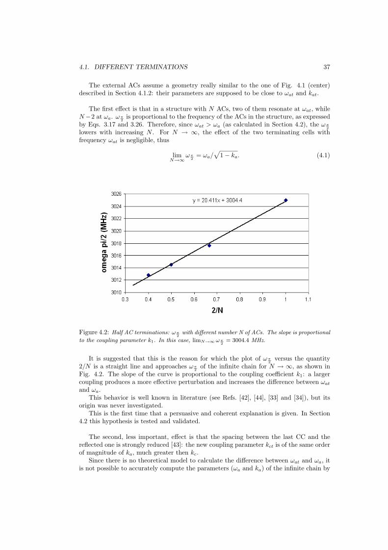
Figure 4.2: Half AC terminations: ω π2
with different number N of ACs. The slope is proportional
to the coupling parameter k1. In this case, limN→∞ ω π2
= 3004.4 MHz.
It is suggested that this is the reason for which the plot of ωπ2
versus the quantity2/N is a straight line and approaches ωπ
2of the infinite chain for N → ∞, as shown in
Fig. 4.2. The slope of the curve is proportional to the coupling coefficient k1: a largercoupling produces a more effective perturbation and increases the difference between ωat
and ωa.This behavior is well known in literature (see Refs. [42], [44], [33] and [34]), but its
origin was never investigated.This is the first time that a persuasive and coherent explanation is given. In Section
4.2 this hypothesis is tested and validated.
The second, less important, effect is that the spacing between the last CC and thereflected one is strongly reduced [43]: the new coupling parameter kct is of the same orderof magnitude of ka, much greater then kc.
Since there is no theoretical model to calculate the difference between ωat and ωa, itis not possible to accurately compute the parameters (ωa and ka) of the infinite chain by
38CHAPTER 4. A NEW STUDY OF SYMMETRY BREAKING IN FINITE CHAINS
measuring half AC terminated structures.
Even an innovative method proposed in Ref. [43] gives inadequate results becauseit takes into account the new kct but not the drastic effect of the broken symmetry.Therefore the precision guaranteed in that article is not reached at all.
The only possibility to get useful results is to compare the measurements with a 3Dsimulation which has exactly the same geometry (Section 7.3).
4.1.4 End Cell termination
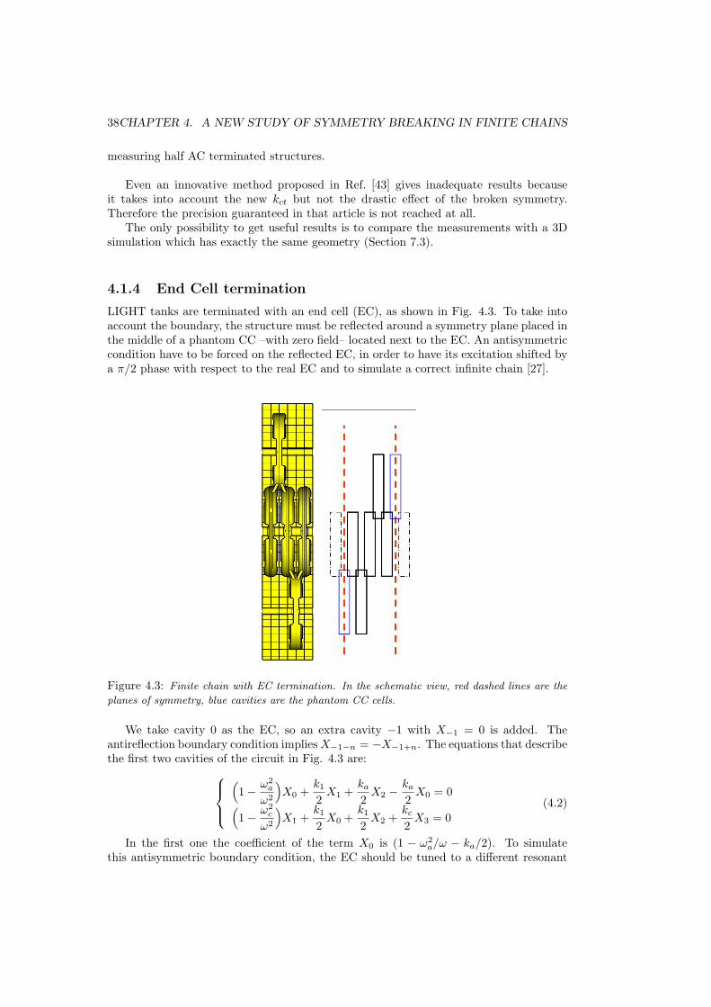
LIGHT tanks are terminated with an end cell (EC), as shown in Fig. 4.3. To take intoaccount the boundary, the structure must be reflected around a symmetry plane placed inthe middle of a phantom CC –with zero field– located next to the EC. An antisymmetriccondition have to be forced on the reflected EC, in order to have its excitation shifted bya π/2 phase with respect to the real EC and to simulate a correct infinite chain [27].
Figure 4.3: Finite chain with EC termination. In the schematic view, red dashed lines are the
planes of symmetry, blue cavities are the phantom CC cells.
We take cavity 0 as the EC, so an extra cavity −1 with X−1 = 0 is added. Theantireflection boundary condition implies X−1−n = −X−1+n. The equations that describethe first two cavities of the circuit in Fig. 4.3 are:
(1− ω2
a
ω2
)X0 +
k1
2X1 +
ka
2X2 −
ka
2X0 = 0(
1− ω2c
ω2
)X1 +
k1
2X0 +
k1
2X2 +
kc
2X3 = 0
(4.2)
In the first one the coefficient of the term X0 is (1 − ω2a/ω − ka/2). To simulate
this antisymmetric boundary condition, the EC should be tuned to a different resonant

4.2. SYMMETRY EFFECT ON ωπ2
IN FINITE CHAIN STRUCTURES 39
frequency ωe that satisfies the relation
1− ω2e
ω2= 1− ω2
a
ω2− ka
2(4.3)
It is not possible to satisfy relation 4.3 for all frequencies, so the ωπ2
is chosen and thecorrect tune for a matched EC is
ω2e = ω2
a
1− ka
2
1− ka= ω2
π2
(1− ka
2
)(4.4)
In a system with matched EC terminations, the Eigenvectors are not described by Eq.3.22 anymore, because the first and last phantom cells have no excitation at all [32] [34][27] [28]. The solution should be sin-like, in order to satisfy the conditions X−1 = 0 andX−1−n = −X−1+n.
The new Eigenvectors that satisfy all boundary conditions are:
X2n = A sin(2n + 1)φ X2n+1 = C sin(2n + 2)φ (4.5)
with
φ =(q + 1)π2N + 2
. (4.6)
If the EC resonant frequency does not match the prescription of Eq. 4.4, the Eigen-vector of the π/2 mode looses the desired form
X π2
= [1, 0,−1, 0, 1, . . .]T (4.7)
and thus the ACs have different stored energy (and electric fields) one with the respectto the others.
In Section 5.2.2 a new method to achieve the correct EC resonant frequency is outlined.
4.2 Symmetry effect on ωπ2
in finite chain structures
4.2.1 Introduction
As described in Section 4.1, ωπ2
is independent of the number of ACs only if the termina-tions of the structure reflect an infinite chain without breaking the symmetry (Fig. 4.1left and center).
In a classical SCL structure with half AC terminations (see Fig. 4.1 right) the bound-ary conditions break the symmetry and ωπ
2depends upon the number of ACs, as shown
in Fig. 4.2.This effect is understandable because of the following consideration. ACs in the middle
of the structure have the correct infinite chain geometry with the coupling slots in the twoopposite semispaces, while boundary ACs have their slot reflected in the same semispace,just as the ACs in the case described in Section 4.1.2.
Therefore, in a structure with N ACs, the two on the boundary resonate at ωat, whilethe N − 2 in the middle at ωa.
40CHAPTER 4. A NEW STUDY OF SYMMETRY BREAKING IN FINITE CHAINS
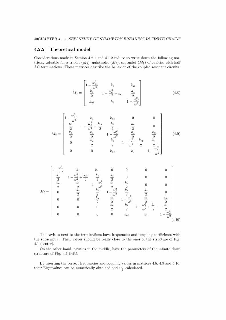
4.2.2 Theoretical model
Considerations made in Section 4.2.1 and 4.1.2 induce to write down the following ma-trices, valuable for a triplet (M3), quintuplet (M5), septuplet (M7) of cavities with halfAC terminations. These matrices describe the behavior of the coupled resonant circuits.
M3 =
1− ω2
at
ω2k1 kat
k1
21− ω2
c
ω2+ kct
k1
2kat k1 1− ω2
at
ω2
(4.8)
M5 =
1− ω2at
ω2k1 kat 0 0
k1
21− ω2
c
ω2+
kct
2k1
2kc
20
ka
2k1
21− ω2
a
ω2
k1
2ka
20
kc
2k1
21− ω2
c
ω2+
kct
2k1
20 0 kat k1 1− ω2
at
ω2
(4.9)
M7 =
266666666666666666664
1− ω2at
ω2k1 kat 0 0 0 0
k1
21− ω2
c
ω2+
kct
2
k1
2
kc
20 0 0
ka
2
k1
21− ω2
a
ω2
k1
2
ka
20 0
0kc
2
k1
21− ω2
c
ω2
k1
2
kc
20
0 0ka
2
k1
21− ω2
a
ω2
k1
2
ka
2
0 0 0ka
2
k1
21− ω2
c
ω2+
kct
2
k1
2
0 0 0 0 kat k1 1− ω2at
ω2
377777777777777777775(4.10)
The cavities next to the terminations have frequencies and coupling coefficients withthe subscript t. Their values should be really close to the ones of the structure of Fig.4.1 (center).
On the other hand, cavities in the middle, have the parameters of the infinite chainstructure of Fig. 4.1 (left).
By inserting the correct frequencies and coupling values in matrices 4.8, 4.9 and 4.10,their Eigenvalues can be numerically obtained and ωπ
2calculated.
4.2. SYMMETRY EFFECT ON ωπ2
IN FINITE CHAIN STRUCTURES 41
4.2.3 Validation of the model
The validation of the model was performed using the cavities of tank 2.
Parameters of the infinite SCL chain (structure in Fig. 4.4 left) and of the chain withall CCs on the same (structure in Fig. 4.4 center) side are given in Table 4.1:
Table 4.1: Parameters of the standard SCL chain (top) and of a chain with all CCs on the same
side (bottom).
ωa ωc k1 ka kc
3027.8 2997.3 0.050 -0.014 0.001
ωat ωct k1 kat kct
3038.4 2997.4 —— -0.009 -0.009
The first set of parameters (Table 4.1, top) was found using the method described inSection 5.2.2 on a quintuplet with half CC terminations (as in Fig. 4.4 left).
The second set (Table 4.1, bottom) was computed by applying the method of Section7.2 on triplets of Fig. 4.4 center and right; k1 cannot be estimated directly with thismethod.
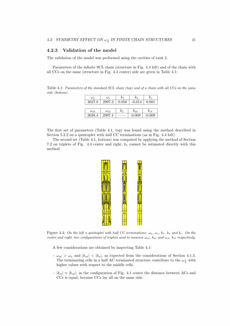
Figure 4.4: On the left a quintuplet with half CC terminations: ωa, ωc, k1, ka and kc. On the
center and right, two configurations of triplets used to measure ωat, kat and ωct, kct respectively.
A few considerations are obtained by inspecting Table 4.1:
- ωat > ωa and |kat| < |ka|, as expected from the considerations of Section 4.1.3.The terminating cells in a half AC terminated structure contribute to the ωπ
2with
higher values with respect to the middle cells.
- |kct| ' |kat|: in the configuration of Fig. 4.1 center the distance between ACs andCCs is equal, because CCs lay all on the same side.

42CHAPTER 4. A NEW STUDY OF SYMMETRY BREAKING IN FINITE CHAINS
- ωct ' ωc because their geometry is the same.
Structures with 3, 5 and 7 cells (terminated by half ACs) were simulated to check thelowering effect on ωπ
2.
Then, by filling matrices 4.8, 4.9 and 4.10 with the data obtained in this section, thevalue of ωπ
2predicted by the model was calculated.
In Table 4.2 the model predictions and the simulated values are shown:
Table 4.2: Comparison between the predictions of the theoretical model and the simulations.
3 cavities 5 cavities 7 cavitiesωπ
2(MHz) simulations 3025.0 3017.6 3014.5
ωπ2
(MHz) model 3025.0 3016.2 3013.5
It is seen that the model gives surprisingly good results, since the error is about 1 MHz:its validity is demonstrated. Another conclusion is that the decrease of ωπ
2with the
increasing number of cavities in a half AC terminated structure is due to the differentresonant frequency and coupling costants of the termination cells.
Chapter 5
New methods to calculatecavities parameters
The detailed study of the boundary conditions on finite chain structures and of the effectof symmetry breaking (discussed in Chapter 4) suggested the development of innovativemethods to calculate cavities parameters.
In this Chapter, after a short overview of simulation codes, a new analytical methodto find out cavities parameters and the correct frequency of the π/2 mode (ωπ/2) ispresented. Moreover, the EC design and an innovative analytical method to get itsresonant frequency ωe are introduced.
In Appendix A a few tips are given to perform correct 3D simulations with CST-Microwave [39].
5.1 Simulation codes
Two different simulation codes, SUPERFISH (SF) and CST-MICROWAVE STUDIO(CST), were used for the design of the cavities. They are both based on a reticulardiscretization of the domain where electrical and magnetic field are defined. They nu-merically solve the partial derivative equations over a grid starting from suitable boundaryconditions.
5.1.1 Superfish
Poisson Superfish, originally developed by the Los Alamos Accelerator Code Group(LAACG), is an electromagnetic field solver in structures with cylindrical symmetry.Therefore it is usually called a 2D code, because from the 2D profile it calculates asymmetric cylindrical cavity.
The program generates a triangular mesh fitted to the boundaries made of differentmaterial. The RF solver iterates the field calculation until it finds a resonant mode.
The assumption of cylindrical symmetry makes the calculation very fast, but all nonsymmetrical items in the structure, such as coupling slots and tuning rods, cannot bedescribed.
43

44 CHAPTER 5. NEW METHODS TO CALCULATE CAVITIES PARAMETERS
However, given a AC geometry, SF finds with a good accuracy many useful parame-ters, such as transit time factor, shunt impedance, quality factor, power dissipated andmaximum electric field.
For these reasons, SF is used for the very first design (when the resonant frequency isroughly estimated, without taking into account the effect of the couplings between cells)and for the optimization of the tank parameters. To perform the final design, a 3D codeas CST is needed.
5.1.2 CST-Microwave Studio
CST is a 3D software based on the Finite Integration Technique (FIT) [39]. It is used tovisualize electric and magnetic fields of the typical normal modes of the cavities and tofind the dispersion curve of the Eigenfrequencies of the system.
The code has many different solvers, but in this thesis only two were used:
- The Eigenmode solver directly calculates the first N resonant frequencies and thecorresponding field patterns by using the JDM (Jacobi Division Method) [39] algo-rithm. In this work it was used to calculate the Eigenmodes of coupled cavities.
- The transient solver is a time domain simulation module capable of solving any kindof so-called S-parameter (parameters associated with the reflection and the trans-mission of electrical signals, see Appendix C). A broad band stimulation enables toobtain with only one calculation the S-parameters for the desired frequency range.In this work it was used to design the correct matching between the waveguide andthe bridge cavity.
5.2 Finding out cavities parameters
5.2.1 Previous method and related problems
The previous design of the cavities made for LIBO was performed following an iterative,time consuming procedure. The most demanding and long part was to find out cavitiesparameters from CST-Microwave simulations.
Minitanks of 3, 5 and 7 cavities, with half AC terminations, were simulated with CST-Microwave and the resonant frequencies of the tank were calculated. Then the cavitiesparameters were obtained by fitting the Eigenfrequencies with the dispersion relation3.25. The calculations were performed with DISPER [23], a program developed by theLos Alamos Group, which is based upon the least square method.
As explained in Section 4.1.3, the parameters of a half AC terminated chain dependupon the number of cavities N . The parameters of the infinite chain were obtained byperforming many simulations with different N and then by plotting the parameters vs.2/N (see Fig. 4.2) so to extrapolate for N →∞.
It is clear that this method is
- time consuming, because many simulations are needed,
- not accurate, since the parameters are calculated by fitting finite chain Eigenvalueswith the dispersion curve of an infinite chain. Moreover, an extrapolation for N →∞ is needed
5.2. FINDING OUT CAVITIES PARAMETERS 45
The detailed study of the importance of symmetries in finite chain structures (seeChapter 4) encouraged the development of a new fast analytical method that cures theseproblems.
5.2.2 A new analytical method to find out the 5 cavity parame-ters of an infinite chain
In this section the new analytical method to find out the 5 cavity parameters of an infinitechain (ωa, ωc, k1, ka, kc) is described. The starting point is that the correct configurationto simulate an infinite chain is a mini-tank with half CC terminations because the coppermirrors that close the structure do not break the symmetry of the chain (Section 4.1.1).
Since there are 5 unknown parameters, 5 independent equations are required to solvethe problem: the smallest structure that can be used is a quintuplet. With a singlesimulation the 5 Eigenfrequencies can be obtained and then the parameters derived ana-lytically.
With this fast method the infinite chain parameters are found directly and not byusing an extrapolation, as in Section 5.2.1.
The system that describes the lumped circuit of a quintuplet terminated with half CCis:
(1− ω2c
ω2)X0 + k1X1 + kcX2 = 0
k1
2X0 + (1− ω2
a
ω2+
ka
2)X1 +
k1
2X2 +
ka
2X3
kc
2X0 +
k1
2X1 + (1− ω2
c
ω2)X2 +
k1
2X3 +
kc
2X4
ka
2X1 +
k1
2X2 + (1− ω2
a
ω2+
ka
2)X3 +
k1
2X4
kcX2 + k1X3 + (1− ω2c
ω2)X4
(5.1)
Note that the last two equations are symmetric to the first two when exchanging4 ↔ 0 and 3 ↔ 1.
Xi=0,...,4 is the square root of the energy in the cavity i for the mode φ and, from Eq.3.22, is equal to:
X2n = B cos 2nφX2n+1 = A cos (2n + 1)φ (5.2)
where φ =πq
2Nis the mode phase and 2N + 1 is the number of cavities.
This system can be completely solved and has five different Eigenvalues ωq and fiveEigenvalues Xq, with q = 0, . . . , 4.
In the present case of 5 cavities the Xi can be written explicitly:
X0 = BX1 = A cos φX2 = B cos 2φX3 = A cos 3φX4 = B cos 4φ
(5.3)

46 CHAPTER 5. NEW METHODS TO CALCULATE CAVITIES PARAMETERS
By substituting the Xi of Eq. 5.3 into the system 5.1 and by considering only its firsttwo equations1, the following system is obtained:
Ak1 cos φ = −B(1− ω2
c
ω2+ kc cos 2φ
)A
((1− ω2
a
ω2+
ka
2) cos 2φ +
ka
2cos 3φ
)= −B
k1
2
(1 + cos 2φ
) (5.4)
By eliminating A and B and manipulating the expression, the dispersion relation is found:
k21 cos2 φ =
(1− ω2
c
ω2+ kc cos 2φ
)(1− ω2
a
ω2+ ka cos 2φ
). (5.5)
As expected, this relation is identical to the one obtained in an infinite chain. Obvi-ously, because φ = πq/2N , it has 5 possible values obtained for q = 0, . . . , 4: φ = 0, π/4,π/2, 3π/4, π. Each value of φ gives an equation, so a system of 5 equations is found.Each of the 5 modes has its own Eigenfrequency (ωl=0,...,4) that can be measured with anetwork analyzer or simulated with a 3D code. The system of 5 independent equationswith 5 unknowns (ωa, ωc, k1, ka, kc) is:
k21 =
(1− ω2
c
ω20
+ kc
)(1− ω2
a
ω20
+ ka
)q = 0
k21 = 2
(1− ω2
c
ω21
)(1− ω2
a
ω21
)q = 1
0 =(1− ω2
c
ω22
− kc
)(1− ω2
a
ω22
− ka
)q = 2
k21 = 2
(1− ω2
c
ω23
)(1− ω2
a
ω23
)q = 3
k21 =
(1− ω2
c
ω24
+ kc
)(1− ω2
a
ω24
+ ka
)q = 4
(5.6)
This system can be easily solved by a homemade Mathematica code.Clearly, this calculation of the parameters of the simulated cavities is much simpler,
faster and accurate than the fitting method used so far. However it should be stressedthat this method cannot be applied to the measurements of real cavities, since the cavitiesdo not have the same resonant frequencies due to mechanical imprecisions.
5.3 End cells
As explained in Section 4.1.4, the EC should be tuned to the resonant frequency
ωe = ωa
√1− ka/2√1− ka
(5.7)
in order to have for the π/2 mode
- a zero E field in the CCs,
- equal energy, and so equal maximum values of electric field in the ACs.1In principle, any couple of equations could be chosen because the system of five equations has five
different Eigenvalues and five orthogonal Eigenvectors. However calculations are easier by consideringthe first two equations.
5.3. END CELLS 47
If this goal is reached, the finite chain perfectly simulates the behavior of an infiniteone (see Section 4.1.4), thus ωπ
2becomes independent of the number of cavities. However,
in practice, a perfect matching is never reached and this effect, even if weak, persists.The difference between the ωπ
2of a 5 ACs chain and of an infinite one is usually about
1− 2 MHz.In practice, the ECs are designed in SF by choosing a target frequency similar to the
one of the CCs. A quintuplet with such ECs is simulated in CST and Eπ/2 is evaluatedalong the beam line and along the center of the CCs. If the maxima of Eπ/2 (the electricfield of π/2 mode) in the ECs are lower (greater) than those in the middle cells, it meansthat ωe is too high (too low). If all the maxima are equal, the end cell has the properfrequency.
Using the analytical method described in Section 5.3.1, from the Eigenfrequenciescalculated with the CST simulation it is possible to get ωe and check its consistency withthe desired value given by Eq. 5.7.
It is also necessary to simulate a seven- and a nine-cavity tank (with ECs) so toconstruct a plot similar to the one of Fig. 4.2. The value of ωπ/2 with the correct tanklength, for example 31 cavities, must be extrapolated by fitting the plot with a straightline.
If the extrapolated value is equal to the one calculated by Eq. 6.8 the tank designis completed. If not, ωa must be changed of the proper quantity to get the correct ωπ/2
value. Of course in the next iteration also ωc and ωe must change to have a closedstopband and a proper termination.
In any case, as already mentioned, the effect of the unavoidable mismatch betweenthe desired and real ωe causes a frequency shift smaller than 1 − 2 MHz and no morethan two iterations are needed to get a good design.
5.3.1 A new analytical method to check the ωe accuracy
The purpose is to find out the EC resonant frequency with a quintuplet. The inputs arethe 5 parameters of an infinite chain, as described in Section 5.2.2, and the π/2 modeEigenfrequency of the EC terminated stack.
The system that describes the lumped circuit of this EC terminated quintuplet is thefollowing:
(1− ω2e
ω2)X0 +
k1
2X1 +
ka
2X2 = 0
k1
2X0 + (1− ω2
c
ω2)X1 +
k1
2X2 +
kc
2X3
ka
2X0 +
k1
2X1 + (1− ω2
a
ω2)X2 +
k1
2X3 +
ka
2X4
kc
2X1 +
k1
2X2 + (1− ω2
c
ω2)X3 +
k1
2X4
ka
2X2 +
k1
2X3 + (1− ω2
e
ω2)X4
(5.8)
Note that the last two equations are symmetric to the first two by exchanging 4 ↔ 0 and3 ↔ 1.
In this case the Eigenvectors are (see Section 4.1.4):

48 CHAPTER 5. NEW METHODS TO CALCULATE CAVITIES PARAMETERS
X0 = D sinφX1 = B sin 2φX2 = A sin 3φX3 = B sin 4φX4 = D sin 5φ
(5.9)
where φ =π(q + 1)2N + 2
is the mode phase, 2N + 1 is the number of cavities, q = 0, . . . , 2N .
Compared to Eq. 5.3, a new constant D has been introduced, to take into accountthe different energy stored in the ECs. The goal is to get A = D, and it is reached if EChas the matched resonant frequency of Eq. 5.7.
The procedure to solve this system is the same used for system 5.1, but this timethree constants A, B and D must be taken into account.
Substituting Eq. 5.9 into the system 5.8 and neglecting the last two equations2, thefollowing system of three equations is obtained:
(1− ω2e
ω2)D sinφ +
k1
2B sin 2φ +
ka
2A sin 3φ = 0
k1
2D sinφ + (1− ω2
c
ω2)B sin 2φ +
k1
2A sin 3φ +
kc
2B sin 4φ
ka
2D sinφ +
k1
2B sin 2φ + (1− ω2
a
ω2)A sin 3φ +
k1
2B sin 4φ +
ka
2D sin 5φ
(5.10)
There are 3 normalization constants (A, B and D) that should be eliminated. Thefirst step is to extract A in each equation and obtain
−A =2
ka sin 3φ
[(1− ω2
e
ω2)E sinφ +
k1
2B sin 2φ
]−A =
1
(1− ω2a
ω2) sin 3φ
[k1
2B(sin 2φ + sin 4φ) + E
ka
2(sinφ + sin 5φ)
]
−A =2
k1 sin 3φ
[B
((1− ω2
c
ω2) sin 2φ +
kc
2sin 4φ
)+ E
k1
2sinφ
] (5.11)
A is eliminated by equating equation 1 with equation 2 and equation 2 with equation3. In the system of two equations only D and B remain. It is possible to play the sametrick used in Section 5.2.2 and obtain, after some calculations, the following dispersionrelation:
k21
2− 2(1− ω2
a
ω2)(1− ω2
c
ω2) + (1− 2 sin2 φ)(k1 − 2(1− ω2
a
ω2)kc)
(1− ω2a
ω2)− ka
2(1 + 5 cos4 φ− 10 cos2 φ sin2 φ + sin4 φ)
= . . .
· · · =
k21
2− ka(1− ω2
c
ω2)− (1− 2sinφ)kakc
ka
2− (1− ω2
e
ω2)
(5.12)
Evaluating this expression is not so simple, but for the particular case of φ = π/2 (for
2The argument is the same used in Section 5.2.2. Any triplet of equations could be chosen, but thefirst three make the calculation faster.
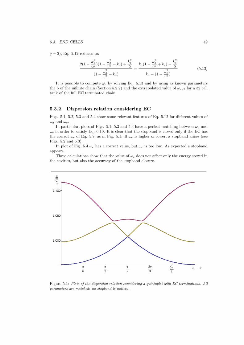
5.3. END CELLS 49
q = 2), Eq. 5.12 reduces to:
2(1− ω2a
ω2)(1− ω2
a
ω2− kc) +
k21
2
(1− ω2a
ω2− ka)
=ka(1− ω2
a
ω2+ kc)−
k21
2
ka − (1− ω2e
ω2)
(5.13)
It is possible to compute ωe by solving Eq. 5.13 and by using as known parametersthe 5 of the infinite chain (Section 5.2.2) and the extrapolated value of ωπ/2 for a 32 celltank of the full EC terminated chain.
5.3.2 Dispersion relation considering EC
Figs. 5.1, 5.2, 5.3 and 5.4 show some relevant features of Eq. 5.12 for different values ofωa and ωe.
In particular, plots of Figs. 5.1, 5.2 and 5.3 have a perfect matching between ωa andωc in order to satisfy Eq. 6.10. It is clear that the stopband is closed only if the EC hasthe correct ωe of Eq. 5.7, as in Fig. 5.1. If ωe is higher or lower, a stopband arises (seeFigs. 5.2 and 5.3).
In plot of Fig. 5.4 ωe has a correct value, but ωc is too low. As expected a stopbandappears.
These calculations show that the value of ωe does not affect only the energy stored inthe cavities, but also the accuracy of the stopband closure.
Figure 5.1: Plots of the dispersion relation considering a quintuplet with EC terminations. All
parameters are matched: no stopband is noticed.
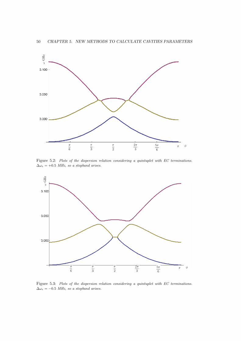
50 CHAPTER 5. NEW METHODS TO CALCULATE CAVITIES PARAMETERS
Figure 5.2: Plots of the dispersion relation considering a quintuplet with EC terminations.
∆ωe = +0.5 MHz, so a stopband arises.
Figure 5.3: Plots of the dispersion relation considering a quintuplet with EC terminations.
∆ωe = −0.5 MHz, so a stopband arises.
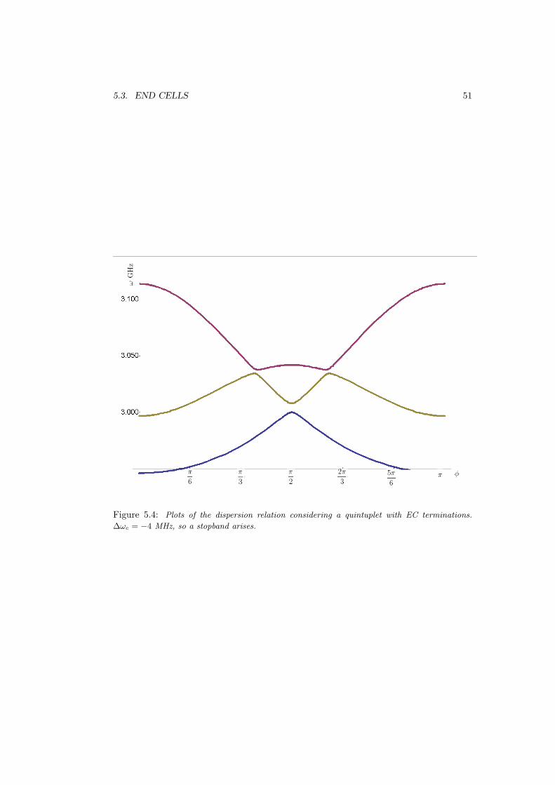
5.3. END CELLS 51
Figure 5.4: Plots of the dispersion relation considering a quintuplet with EC terminations.
∆ωc = −4 MHz, so a stopband arises.

52 CHAPTER 5. NEW METHODS TO CALCULATE CAVITIES PARAMETERS

Chapter 6
Tank design algorithm andresults
The innovative methods studied in Chapter 5 made possible to develop a new algorithmfor the tank design.
In this Chapter, after a short overview of cavities geometry, nose parameters and cou-pling slot optimization are examined. The correct frequency of the π/2 mode (ωπ/2) isquickly obtained by applying the method described in Section 5.2.2. Finally the designparameters and a study about mechanical tolerances of Tank 1 and 2 are presented.
6.1 Cell geometry overview
Figure 6.1: A 2D sketch of the cells is given. Noses are placed in the capacitive region, while
the coupling slot that connects the two cavities is in the distal magnetic part.
The geometries of the AC and the CC are shown in Fig. 6.1. The general purpose ofthe design is to excite a strong longitudinal electric field on the beam axis of the AC.
The nose shape, smaller and sharper in AC then in CC, is critically important to havegood accelerating parameters. The optimization procedure is described in Section 6.4.
Each cavity can be roughly subdivided into two parts:
53
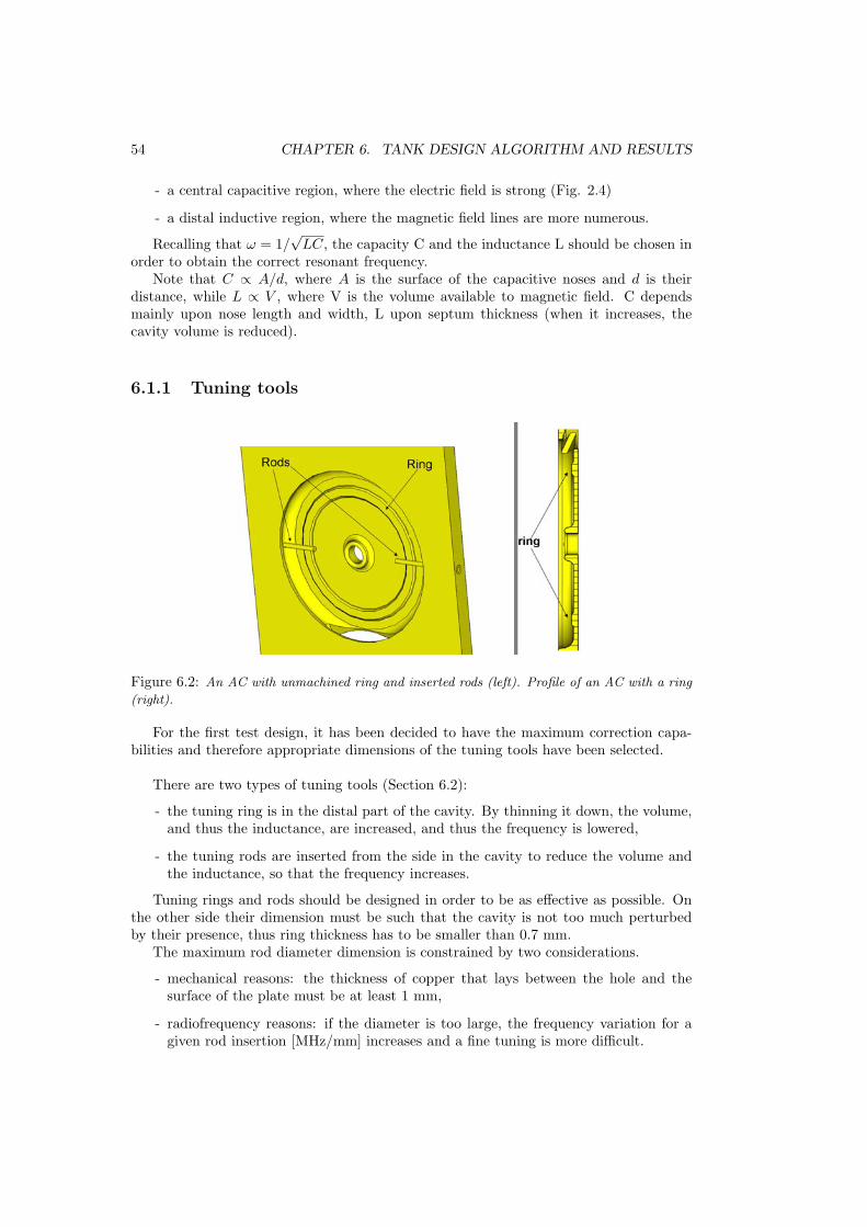
54 CHAPTER 6. TANK DESIGN ALGORITHM AND RESULTS
- a central capacitive region, where the electric field is strong (Fig. 2.4)
- a distal inductive region, where the magnetic field lines are more numerous.
Recalling that ω = 1/√
LC, the capacity C and the inductance L should be chosen inorder to obtain the correct resonant frequency.
Note that C ∝ A/d, where A is the surface of the capacitive noses and d is theirdistance, while L ∝ V , where V is the volume available to magnetic field. C dependsmainly upon nose length and width, L upon septum thickness (when it increases, thecavity volume is reduced).
6.1.1 Tuning tools
Figure 6.2: An AC with unmachined ring and inserted rods (left). Profile of an AC with a ring
(right).
For the first test design, it has been decided to have the maximum correction capa-bilities and therefore appropriate dimensions of the tuning tools have been selected.
There are two types of tuning tools (Section 6.2):
- the tuning ring is in the distal part of the cavity. By thinning it down, the volume,and thus the inductance, are increased, and thus the frequency is lowered,
- the tuning rods are inserted from the side in the cavity to reduce the volume andthe inductance, so that the frequency increases.
Tuning rings and rods should be designed in order to be as effective as possible. Onthe other side their dimension must be such that the cavity is not too much perturbedby their presence, thus ring thickness has to be smaller than 0.7 mm.
The maximum rod diameter dimension is constrained by two considerations.
- mechanical reasons: the thickness of copper that lays between the hole and thesurface of the plate must be at least 1 mm,
- radiofrequency reasons: if the diameter is too large, the frequency variation for agiven rod insertion [MHz/mm] increases and a fine tuning is more difficult.

6.2. INTRODUCTION TO TANK DESIGN 55
6.2 Introduction to tank design
The purposes of tank design are the following:
1. to obtain an high ZT 2 (effective shunt impedance for unit of length), so that thepower consumption is reduced for a given linac length,
2. to obtain an high Q (quality factor), Sec. 2.2.3,
3. to get an Emax (the maximum electric field in the cavity) such that the Kilpatrickparameter is smaller than 1.7− 2, Sec. 2.2.3,
4. to provide the cavities with a dynamic tuning range (through rings and rods) aslarge as possible,
5. to obtain a spacing between adjacent modes as large as possible, Sec. 3.4.1,
6. to achieve 2998.5 MHz as resonant π/2 frequency of the whole tank,
7. to have a stopband smaller than 1 MHz, Sec. 3.4.1,
8. to find the right end cell frequency, Sec. 4.1.4.
The first three goals are obtained with the SUPERFISH code [12] by changing thenose parameters (inner corner radius Ri, outer corner radius Ro, cone angle αc - see Fig.6.3): usually sharper edges improve ZT 2 but raise Emax as well, so an optimum has tobe found. Moreover the optimum depends on the resonant frequency of the cavity, sothis operation has to be done approximatively a first time and has to be repeated afterhaving found the correct ωπ
2.
The fourth goal is obtained by a combination of the 2D SUPERFISH and the 3DCST-Microwave codes for the ring part and by 3D CST-Microwave code only for the rodpart. The dynamical range depends slightly on the frequency: after having found theright resonant frequency, the tuning range must be checked again. The linearity of thetuning effect must be tested as well, in order to have the knowledge needed to begin thefirst tuning step by machining the ring.
The fifth goal is obtained with CST simulations. Given a fix number of cells per tank,the spacing is proportional to the first neighbor coupling value k1, thus special ovoidalslots have been designed and tested in order to increase the coupling with respect to theprevious design and reach k1 ' 0.05.
The sixth and seventh goals are obtained by using a combination of SUPERFISHand CST-Microwave codes. The 2D code gives the rough resonant frequency of the ACand the CC without considering k1, ka and kc (which are respectively the first neighbor,AC→AC and CC→CC coupling values). In order to consider these factors, which greatelyinfluence the resonant frequency, a 3D simulation is required. The decrease of the ωπ/2
at the increasing of the number of cells should also be studied and evaluated.The last problem is strictly connected with the previous one. Closing the end cell in
a proper way has to be studied with a 3D simulation. The best is to obtain an E field ofthe π/2 mode (named Eπ
2) as low as possible in the middle of the CC and with all the
maxima having the same values.

56 CHAPTER 6. TANK DESIGN ALGORITHM AND RESULTS
6.3 Guessing the frequency
The first step of the design is to make an educated guess of the SUPERFISH frequenciesof AC and CC. Since SF works in a cylindrical symmetric space, the perturbation givenby the coupling slots is not considered. A slot in a cavity causes a frequency loweringeffect ∆fslot due to the increase of volume available for magnetic field and due to thecoupling with neighbor cells. Therefore the SF goal frequency is much higher than theeffective 3D one.
If data from previous 3D simulations are not available, a reasonable SUPERFISHfrequency can be estimated through the formula given in Ref. [36]:
fSF = fgoal
√1− ka + ∆fslot (6.1)
∆fslot can be estimated supposing that the frequency shift is proportional to the couplingparameter k1: as explained in Ref. [37], ∆fslot = k1fnoslot.
As an example, in the case of the 1st tank, with an interaxes distance of 62 mm,k1 ' 0.05 and ka ' 0.01, the fSF is about 3130 MHz for AC and 3100 MHz for CC.
To test the accuracy of the guess, a 3D simulation of a quintuplet terminated withhalf CC should be run. The analytical method to find out the cavity parameters (ωa, ωc,k1, ka, kc) from the five Eigenfrequencies is described in Section 5.2.2. The final ωπ/2 foran infinite chain (which will be only about 1 MHz lower than the real one, see Section5.3) is calculated by:
ωπ/2 =ωa√
1− ka
=ωc√
1− kc
(6.2)
ωa, ωc, ka and kc should be such to bring ωπ2
to the target value (Sec. 6.6.2) with aclosed stopband.
6.4 Cavity and AC nose design optimization
The nose geometry must be optimized in order to get the maximum ZT 2 and Q valuesat a given Emax and cell resonant frequency.
The septum thickness (s) should be as thin as possible but must satisfy the mechanicalconstrain to be larger than 3 mm to avoid problems during the brazing procedure.
The bore radius (Rb) is chosen according to beam dynamic studies. A good com-promise between a good ZT 2 and a high enough transmittance of the beam is Rb = 3.5mm [8].
The diameter (D) affects largely the final ZT 2. A study of ZT 2 and Q with differentD was performed. The optimum value is D = 7 mm.
The parameters involved in the optimization (shown in Fig. 6.3) are:
- Ri: when it decreases, both ZT 2 and Emax increase because of the sharp edge.
- F : when it increases, ZT 2, Q and Emax decrease. Typical value ≤ 0.4 mm.
- Ro: it affects both ZT 2 and Emax because it can produce a sharp edge (just as inthe Ri case).
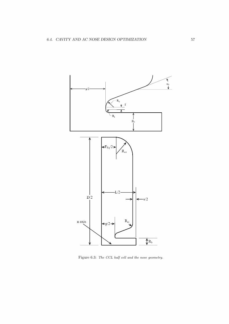
6.4. CAVITY AND AC NOSE DESIGN OPTIMIZATION 57
Figure 6.3: The CCL half cell and the nose geometry.
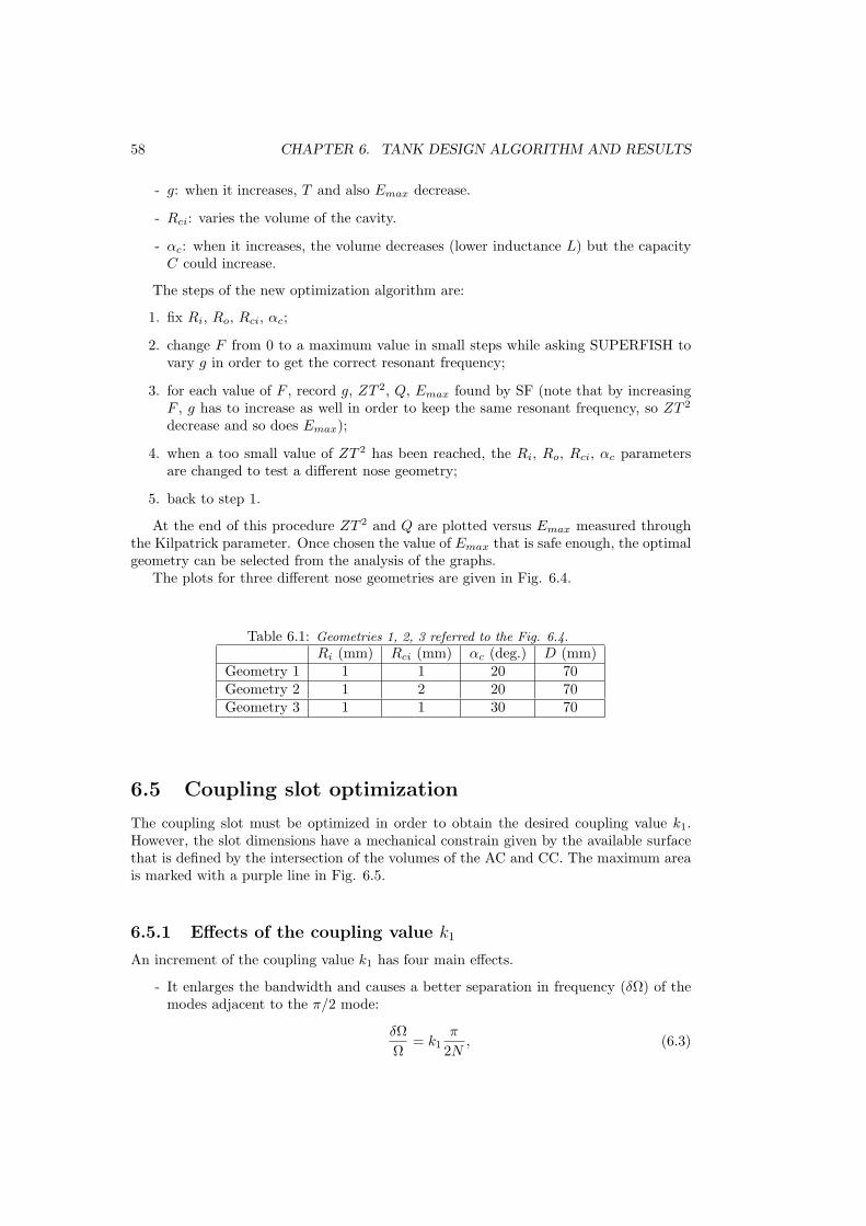
58 CHAPTER 6. TANK DESIGN ALGORITHM AND RESULTS
- g: when it increases, T and also Emax decrease.
- Rci: varies the volume of the cavity.
- αc: when it increases, the volume decreases (lower inductance L) but the capacityC could increase.
The steps of the new optimization algorithm are:
1. fix Ri, Ro, Rci, αc;
2. change F from 0 to a maximum value in small steps while asking SUPERFISH tovary g in order to get the correct resonant frequency;
3. for each value of F , record g, ZT 2, Q, Emax found by SF (note that by increasingF , g has to increase as well in order to keep the same resonant frequency, so ZT 2
decrease and so does Emax);
4. when a too small value of ZT 2 has been reached, the Ri, Ro, Rci, αc parametersare changed to test a different nose geometry;
5. back to step 1.
At the end of this procedure ZT 2 and Q are plotted versus Emax measured throughthe Kilpatrick parameter. Once chosen the value of Emax that is safe enough, the optimalgeometry can be selected from the analysis of the graphs.
The plots for three different nose geometries are given in Fig. 6.4.
Table 6.1: Geometries 1, 2, 3 referred to the Fig. 6.4.
Ri (mm) Rci (mm) αc (deg.) D (mm)Geometry 1 1 1 20 70Geometry 2 1 2 20 70Geometry 3 1 1 30 70
6.5 Coupling slot optimization
The coupling slot must be optimized in order to obtain the desired coupling value k1.However, the slot dimensions have a mechanical constrain given by the available surfacethat is defined by the intersection of the volumes of the AC and CC. The maximum areais marked with a purple line in Fig. 6.5.
6.5.1 Effects of the coupling value k1
An increment of the coupling value k1 has four main effects.
- It enlarges the bandwidth and causes a better separation in frequency (δΩ) of themodes adjacent to the π/2 mode:
δΩΩ
= k1π
2N, (6.3)
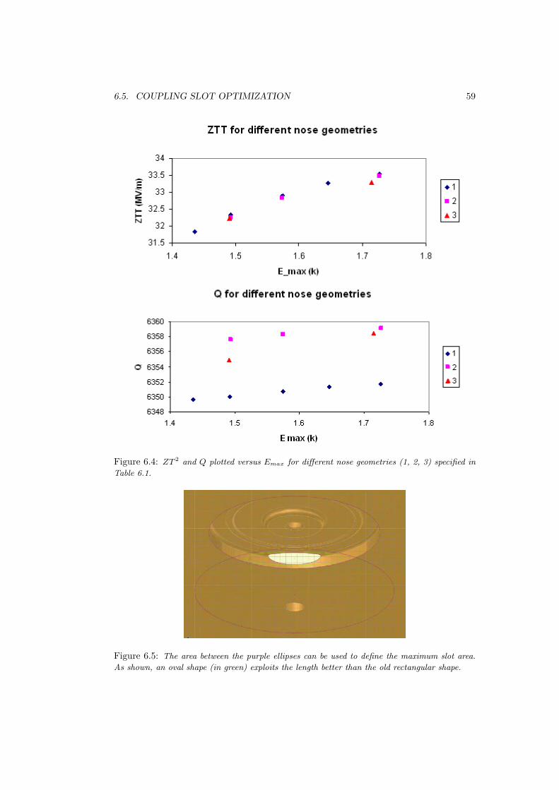
6.5. COUPLING SLOT OPTIMIZATION 59
Figure 6.4: ZT 2 and Q plotted versus Emax for different nose geometries (1, 2, 3) specified in
Table 6.1.
Figure 6.5: The area between the purple ellipses can be used to define the maximum slot area.
As shown, an oval shape (in green) exploits the length better than the old rectangular shape.

60 CHAPTER 6. TANK DESIGN ALGORITHM AND RESULTS
where 2N + 1 is the number of cavities in the chain.
- It increases the dissipated power P . The shunt impedance ZT 2 looses about 3% foreach 1% increment of k1 (Ref. [12]).
- It may cause a drop of the Q value because of the increased power dissipation:
Q =ω
∆ω=
ωU
P (k1)(6.4)
where ∆ω is the width of the mode at −3 dB from the peak.
- It makes the whole system less sensible to tuning errors of single cavities (see Section3.4.1).
The aims are the following ones:
1. to have the quantity∆ω
δΩas small as possible in order not to excite modes that
are different from the π/2. Since both ∆ω and δΩ increase with increasing k1, anoptimum has to be found;
2. to obtain a ZT 2 not too low (at least 30 MΩ/m) in order to have a reasonablepower consumption (less than 1.3 kW per tank);
3. to have k1 as big as possible in order to make the system less sensible to tuningerrors.
6.5.2 Choice of k1
Firstly, the effect of k1 on the quantityδΩ∆ω
has to be investigated.
α =δΩ∆ω
=k1πQ(k1)
2N(6.5)
and the maximum can be calculated by equating to zero the first derivative:
d
dk1
( δΩ∆ω
)=
π
2N
δ
δk1
(k1Q(k1)
)=
π
2N
(Q(k1) + k1
δQ(k1)δk1
). (6.6)
Thus the optimum k1 satisfies
k1 ' −Q
δQ/δk1(6.7)
From the the results of CST simulations with coupling slots of different shape, Q '2400 and δQ/δk1 ' −27000. The best value of k1 to increase the separation betweenadjacent modes is about k1 ' 0.09. In Fig. 6.6 a plot of δΩ/∆ω for different values of k1
is shown.Secondly, the effect of k1 on ZT 2 must be studied. ZT 2 at 30 MeV is usually very low
in SCL with respect to other linear accelerators (for example DTL), due to the squeezedgeometry of AC (see Ref. [28]). For tank 1 and tank 2, ZT 2 is about 35 MΩ/m, neglectinglosses due to coupling parameter. Therefore, using the relation given in Section 6.5.1, k1
should be smaller than 0.05 in order to have ZT 2 > 30 MΩ/m.
These considerations, combined well to the mechanical constrain of Section 6.5, drovethe choice of k1 ' 0.05.

6.6. TARGET FREQUENCY AND STOPBAND 61
Figure 6.6: α = δΩ/∆ω for different values of k1. The maximum is reached for k1 ' 0.09.
6.5.3 Oval slot proposal
The coupling slot of the previous design was rectangular with smoothed angles. Thisgeometry does not make full use of the natural hole (more or less elliptical) that jointsCC to AC (Fig. 6.5). Since the k1 parameter has a dependence on l3 (Eq. 3.12), toimprove the coupling it is important to have l as large as possible. Thus an oval shapeof the slot has been considered and tested.
While the previous shape provided k1 = 0.033, the oval one guarantees k1 = 0.052,because it can exploit better the full available area (purple border in Fig. 6.5) and obtaina larger l. The Q factor does not decrease significantly, so the new shape has been chosen.The drawback is that ka and kc are increased too.
From a practical point of view, it has to be underlined that the construction of slots ofsuch shape cannot be made with a milling machine because the smallest spindle availableis 2 mm. Only an EDM machining can be used.
6.6 Target frequency and stopband
Before the definition of the target frequency, the effect of tuning facilities has to be accu-rately calculated. Then the target frequency is set and the parameters of ACs and CCsare chosen in order to reach the desired configuration with zero stopband.
6.6.1 Tuning facilities effect
Ring
The quickest way to get an estimation of ring effect is to compute cavities parameterswith and without the ring. The method used for the computation is the one described inSection 5.2.2: only a simulation per geometry is needed.
The frequency effect ∆ωring is obtained as the difference between the two values (withand without the ring) of ωa (for AC) and ωc (for CC).
Usually the thinning of a big ring raises the frequency by about 15− 20 MHz.

62 CHAPTER 6. TANK DESIGN ALGORITHM AND RESULTS
Since the ring frequency shift is basically due to volume reduction, the outer part ofthe cavity is more sensitive because the diameter (and consequently the volume) is larger.
The sensitivity of the ring should be about 3 MHz/0.1 mm, so that a machining of 20µm lowers the frequency by about 500 kHz.
Rod
In order to determine the effect of the rods, the most direct way is to calculate ωa andωc with the method of Section 5.2.2 for different geometries, by inserting the tuning rodsstep by step into the cavities. ∆ωrod is the maximum variation of ωa and ωc.
Usually the maximum effect of the rods insertion is a frequency increase of 10 − 15MHz.
It has to be considered that usually when the rods are inserted for more than 10− 12mm they enter the capacitive region and produce the opposite effect by lowering thefrequency due to capacity increase.
Moreover the electric field lines are deformed due to the proximity of the copper rodsand this effect could perturb the longitudinal and transversal dynamics of the beam.
6.6.2 Choosing the target frequency
The final target frequency for the 16 AC tank with EC terminations is
ωTARGET = 2998.5 +∆ωring
2− ∆ωrod
2+ 0.5 + 1 (MHz) (6.8)
- +2998.5 MHz is the klystron frequency;
- half of the ring effect must be added and half of the rod subtracted because theoptimum is set to be with half ring cut away and half of the rod inserted;
- the design is performed at a temperature Td = 24 deg, but the operating temper-ature will be To = 34deg. The copper deformation due to a temperature shift of+10 deg produces a frequency change of −0.5 MHz (Ref. [11]). Therefore the designfrequency has to include a +0.5 MHz term;
- +1 MHz should be added to consider the frequency lowering effect described inSection 5.3,
6.6.3 ωπ/2 and stopband
The value of ωa must be such that
ωa√1− ka
= ωTARGET , (6.9)
where ωa and ka are obtained with the method of Section 5.2.2.To obtain the correct resonant frequencies, an iterative procedure is performed. In
each step, the geometry of the AC is chosen and ωa is computed first with SUPERFISHand then with the the method of Section 5.2.2, that is based on CST simulations andgives the correct parameter of the infinite chain.

6.7. PARAMETERS OF THE FOUR TANKS 63
For instance, if the SUPERFISH value (ωSF = 3030 MHz) corresponds to an infinitechain parameter 10 MHz lower than the desired one, in the next step the good value forSUPERFISH is 3040 MHz.
Then a new CST simulation is performed with the new design and the new parametersare calculated. This iterative procedure goes on until a good result is obtained.
It should be stressed that, since the CST simulation has an accuracy of about 2 − 3MHz (see A and [39]), a 1 MHz accuracy is enough.
In the same iterative way, the right CC resonant frequency is chosen in order to satisfythe relation
SB =ωa√
1− ka
− ωc√1− kc
= 0 (6.10)
where SB is the stop–band.
6.7 Parameters of the four Tanks
The final parameters of the four tanks of the First Unit are shown in the Tables 6.2, 6.3and 6.4:
Table 6.2: Cavities parameters for tank 1 and 2.
ωa (GHz) ωc (GHz) k1 ka kc Qa Qc
TANK 1 3026.1 3001.7 0.0519 -0.0145 0.001 5507 4851TANK 2 3023.1 2998.9 0.0515 -0.0142 0.001 5740 5041
Table 6.3: Tuning facilities effects for tank 1 and 2. Since there are two rods in each half cavity,
to obtain the overall tuning rods effect, the value in this Table must be multiplied by 2. In Figs.
6.7 and 6.8 an accurate plot of tuning sensitivity is shown.
AC (MHz) CC (MHz)∆ωring ∆ωrod ∆ωring ∆ωrod
TANK 1 -22.1 +6.5 -28.0 +9.4TANK 2 -21.4 +6.3 -24.5 +8.5
Graphs in in Figs. 6.7 and 6.8 show the effect on the frequency of the tuning facilities.They are used to perform an accurate tuning, as described in Section 7.1.
The performance parameters of tank 1 and 2 are shown in Table 6.4:
Table 6.4: Performance parameters for tank 1 and 2.
E0 (MV/m) ZT 2 (MΩ/m) T Emax (k) Q0 P0 (MW) N L (mm)
T 1 15.65 27.420 0.83 1.50 5170 1.252 16 201.6T 2 15.65 30.685 0.84 1.68 5390 1.200 16 209.6
The meanings of all parameters are explained in Chapter 2.
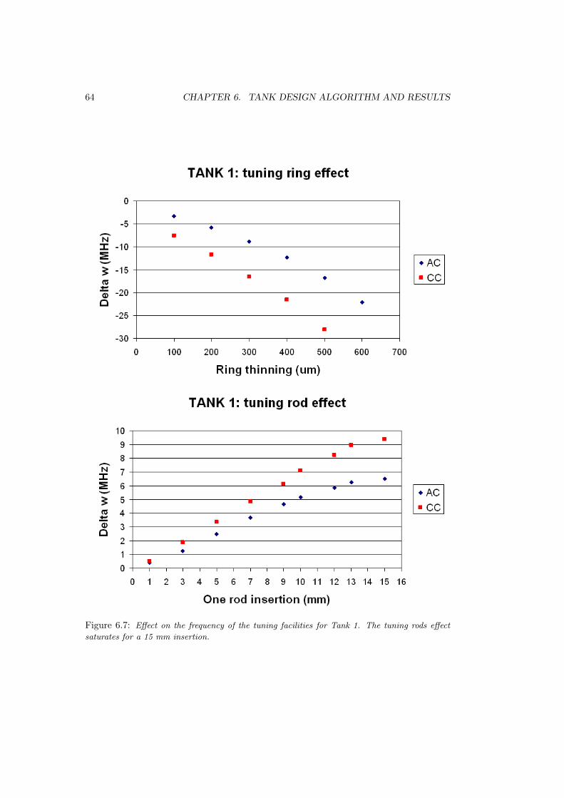
64 CHAPTER 6. TANK DESIGN ALGORITHM AND RESULTS
Figure 6.7: Effect on the frequency of the tuning facilities for Tank 1. The tuning rods effect
saturates for a 15 mm insertion.
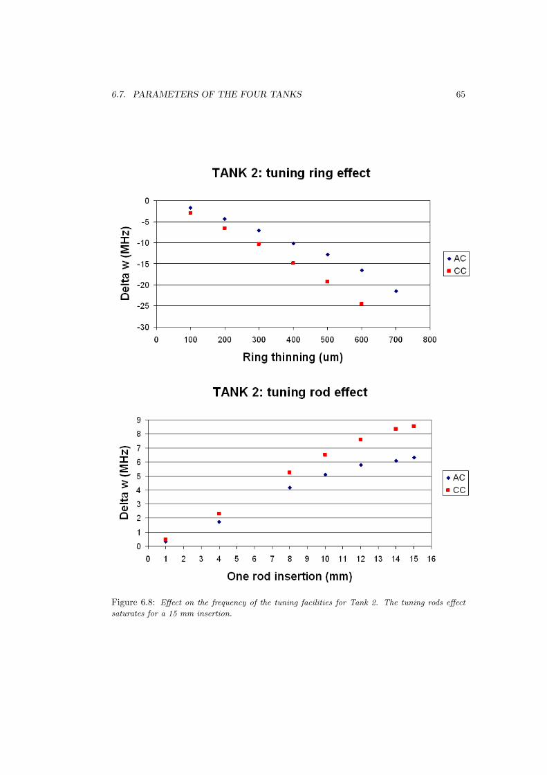
6.7. PARAMETERS OF THE FOUR TANKS 65
Figure 6.8: Effect on the frequency of the tuning facilities for Tank 2. The tuning rods effect
saturates for a 15 mm insertion.

66 CHAPTER 6. TANK DESIGN ALGORITHM AND RESULTS
6.7.1 Effects of mechanical tolerances
It is of critical importance to test the frequency shift due to mechanical tolerances, sincemore stringent requests increase the manufacturing costs.
The study split the cavities in two independent subregions: the nose and the distalpart. Effects of mechanical tolerances were investigated for the two parts separately. Itwas proven that, when tolerances on both parts are considered at the same time, in theworst case the overall error is the sum of the two.
In Tables 6.5 and 6.6 the effects of the mechanical tolerances on the nose and on thedistal part are shown respectively.
Table 6.5: Frequency effects of the mechanical tolerancies of the nose.
Nose Tank 1 Tank 2tolerance (µm) |∆ωa| (MHz) |∆ωc| (MHz) |∆ωa| (MHz) |∆ωc| (MHz)
5 0.9 1.9 0.7 1.710 2.1 4.2 2.4 3.620 4.8 8.3 6.3 7.4
Table 6.6: Frequency effects of the mechanical tolerancies of the distal part.
Distal part Tank 1 Tank 2tolerance (µm) |∆ωa| (MHz) |∆ωc| (MHz) |∆ωa| (MHz) |∆ωc| (MHz)
5 0.8 0.9 0.4 1.010 0.8 2.2 1.8 1.320 1.0 3.8 2.3 3.1
The shape of the electric field in AC depends on the nose geometry, thus mechanicaltolerance of the nose is a sensitive parameter for both resonant frequency and beamdynamics.
If dispersion among different cells is kept within 10 MHz, the available tuning facilitiesare sufficient to bring each cavity to the proper resonant frequency.
The choice to request a 5 µm tolerance for the nose and 20 µm for the distal part is areasonable balance between performances and costs. In this way a precision of ±5 MHzis assured.
If such precision is really obtained, a design without tuning rings could be considered.This possibility is at present under investigation (see Section 9.2).

Chapter 7
Measurements of the tankparameters
7.1 Measurements and tuning overview
Measuring cavities parameters is a critical aspect in accelerator construction. Demandingmechanical precisions (between 5 − 20 µm, see Section 6.7) are requested to the manu-facturers. But this is not sufficient, since errors of a few µm induce frequency mistuningof about 5 − 15 MHz. At the end of the tuning procedure, accuracies in the frequencybetter than 200− 300 kHz are requested.
Large mistuning of the cavities could bring to a non uniformity of electric fields be-cause the Eigenvectors of Eq. 3.22 would not have the same amplitude [18] [26].
As explained in Section 6.1.1, three tuning tools are available for each half cavity: onetuning ring and two tuning rods.
After the manufacturing of the plates, each cavity is measured with the method ex-plained in Section 7.2 (a technical guide is provided in Appendix B). Frequencies shouldbe dispersed around a mean value with a standard deviation of about 10 MHz, given byrandom mechanical imperfections. This dispersion is reduced to 200 kHz by thinning therings in successive mechanical operations. To achieve this, high precision measurementsare needed.
After brazing the whole tank, the lateral tuners are necessary to bring the ACs andthe CCs resonant frequencies to the design values.
The tuners of the same tank are mechanically connected and thus are inserted alltogether by the same amount, in order to bring ωa and ωc of the tank to the desired val-ues. For this reason individual tuning of the cavities must be performed with the ring only.
7.2 Measurements in different configurations
To measure the AC and the CC resonant frequencies accurately, two configurations areused: triplets with half CC terminations and triplets with half AC terminations (Fig.7.1).
67
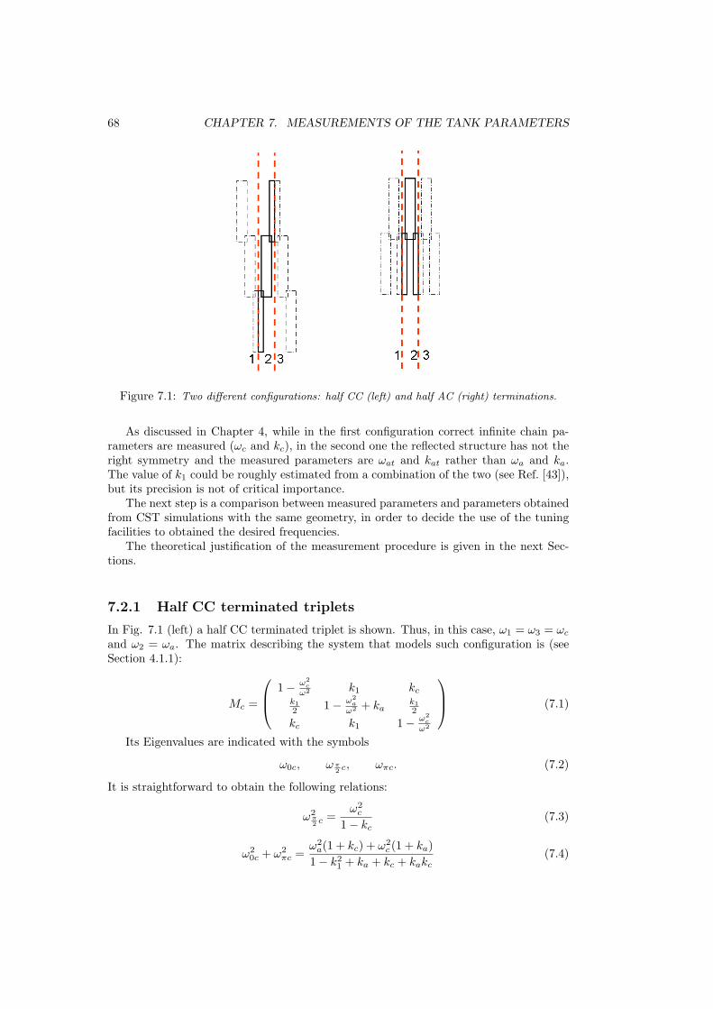
68 CHAPTER 7. MEASUREMENTS OF THE TANK PARAMETERS
Figure 7.1: Two different configurations: half CC (left) and half AC (right) terminations.
As discussed in Chapter 4, while in the first configuration correct infinite chain pa-rameters are measured (ωc and kc), in the second one the reflected structure has not theright symmetry and the measured parameters are ωat and kat rather than ωa and ka.The value of k1 could be roughly estimated from a combination of the two (see Ref. [43]),but its precision is not of critical importance.
The next step is a comparison between measured parameters and parameters obtainedfrom CST simulations with the same geometry, in order to decide the use of the tuningfacilities to obtained the desired frequencies.
The theoretical justification of the measurement procedure is given in the next Sec-tions.
7.2.1 Half CC terminated triplets
In Fig. 7.1 (left) a half CC terminated triplet is shown. Thus, in this case, ω1 = ω3 = ωc
and ω2 = ωa. The matrix describing the system that models such configuration is (seeSection 4.1.1):
Mc =
1− ω2c
ω2 k1 kc
k12 1− ω2
a
ω2 + kak12
kc k1 1− ω2c
ω2
(7.1)
Its Eigenvalues are indicated with the symbols
ω0c, ωπ2 c, ωπc. (7.2)
It is straightforward to obtain the following relations:
ω2π2 c =
ω2c
1− kc(7.3)
ω20c + ω2
πc =ω2
a(1 + kc) + ω2c (1 + ka)
1− k21 + ka + kc + kakc
(7.4)

7.2. MEASUREMENTS IN DIFFERENT CONFIGURATIONS 69
ω20cω
2πc =
ω2aω2
c
1− k21 + ka + kc + kakc
(7.5)
Deriving ω2a from Eq. 7.4 and substituting it into Eq. 7.5, a linear relation is obtained:
yc = Acxc + Bc (7.6)
whereyc = ω2
0cω2πc, (7.7)
xc = ω20c + ω2
πc, (7.8)
Ac =ω2
c
1 + kc, (7.9)
Bc = − ω4c (1 + ka)
(1− k21 + ka + kc + kakc)(1 + kc)
. (7.10)
So, by perturbing the AC it is possible to plot different couples of values xc, yc and toderive Ac and Bc from a linear fit (see in Appendix B).
Finally, from Eqs. 7.9 and 7.3: Ac =
ω2c
1 + kc
ωπ2 c =
ω2c
1− kc
(7.11)
one obtains the unknown parameters wc and kc.
7.2.2 Half AC terminated triplets
The same method can be applied to the circuit of Fig. 7.1 (right). In this case we haveω1 = ω3 = ωat, ω2 = ωc and the linear relation is:
ya = Aaxa + Ba, (7.12)
whereya = ω2
0aω2πa, (7.13)
xa = ω20a + ω2
πa, (7.14)
Aa =ω2
at
1 + kat, (7.15)
Ba = − ω4at(1 + kct)
(1− k21 + kat + kct + katkct)(1 + kct)
(7.16)
where ωa, ka and kct are the resonant frequencies and coupling constants introducedin 4.1.3, different from the infinite chain parameters.
By solving the system of equations:Aa =
ω2at
1 + kat
ωπ2 a =
ω2at
1− kat
(7.17)
the two unknown parameters wat and kat are easily obtained.
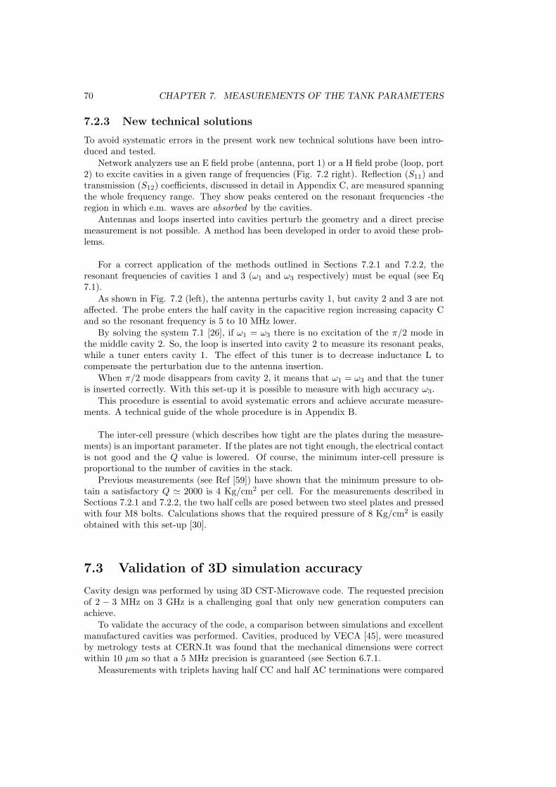
70 CHAPTER 7. MEASUREMENTS OF THE TANK PARAMETERS
7.2.3 New technical solutions
To avoid systematic errors in the present work new technical solutions have been intro-duced and tested.
Network analyzers use an E field probe (antenna, port 1) or a H field probe (loop, port2) to excite cavities in a given range of frequencies (Fig. 7.2 right). Reflection (S11) andtransmission (S12) coefficients, discussed in detail in Appendix C, are measured spanningthe whole frequency range. They show peaks centered on the resonant frequencies -theregion in which e.m. waves are absorbed by the cavities.
Antennas and loops inserted into cavities perturb the geometry and a direct precisemeasurement is not possible. A method has been developed in order to avoid these prob-lems.
For a correct application of the methods outlined in Sections 7.2.1 and 7.2.2, theresonant frequencies of cavities 1 and 3 (ω1 and ω3 respectively) must be equal (see Eq7.1).
As shown in Fig. 7.2 (left), the antenna perturbs cavity 1, but cavity 2 and 3 are notaffected. The probe enters the half cavity in the capacitive region increasing capacity Cand so the resonant frequency is 5 to 10 MHz lower.
By solving the system 7.1 [26], if ω1 = ω3 there is no excitation of the π/2 mode inthe middle cavity 2. So, the loop is inserted into cavity 2 to measure its resonant peaks,while a tuner enters cavity 1. The effect of this tuner is to decrease inductance L tocompensate the perturbation due to the antenna insertion.
When π/2 mode disappears from cavity 2, it means that ω1 = ω3 and that the tuneris inserted correctly. With this set-up it is possible to measure with high accuracy ω3.
This procedure is essential to avoid systematic errors and achieve accurate measure-ments. A technical guide of the whole procedure is in Appendix B.
The inter-cell pressure (which describes how tight are the plates during the measure-ments) is an important parameter. If the plates are not tight enough, the electrical contactis not good and the Q value is lowered. Of course, the minimum inter-cell pressure isproportional to the number of cavities in the stack.
Previous measurements (see Ref [59]) have shown that the minimum pressure to ob-tain a satisfactory Q ' 2000 is 4 Kg/cm2 per cell. For the measurements described inSections 7.2.1 and 7.2.2, the two half cells are posed between two steel plates and pressedwith four M8 bolts. Calculations shows that the required pressure of 8 Kg/cm2 is easilyobtained with this set-up [30].
7.3 Validation of 3D simulation accuracy
Cavity design was performed by using 3D CST-Microwave code. The requested precisionof 2 − 3 MHz on 3 GHz is a challenging goal that only new generation computers canachieve.
To validate the accuracy of the code, a comparison between simulations and excellentmanufactured cavities was performed. Cavities, produced by VECA [45], were measuredby metrology tests at CERN.It was found that the mechanical dimensions were correctwithin 10 µm so that a 5 MHz precision is guaranteed (see Section 6.7.1.
Measurements with triplets having half CC and half AC terminations were compared
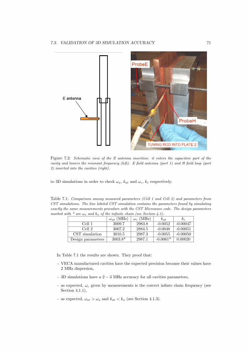
7.3. VALIDATION OF 3D SIMULATION ACCURACY 71
Figure 7.2: Schematic view of the E antenna insertion: it enters the capacitive part of the
cavity and lowers the resonant frequency (left). E field antenna (port 1) and H field loop (port
2) inserted into the cavities (right).
to 3D simulations in order to check ωa, kat and ωc, kc respectively.
Table 7.1: Comparison among measured parameters (Cell 1 and Cell 2) and parameters from
CST simulations. The line labeled CST simulation contains the parameters found by simulating
exactly the same measurements procedure with the CST Microwave code. The design parameters
marked with * are ωa and ka of the infinite chain (see Section 4.1).
ωat (MHz) ωc (MHz) kat kc
Cell 1 3009.7 2983.8 -0.0052 -0.00047Cell 2 3007.2 2884.5 -0.0048 -0.00051
CST simulation 3010.5 2987.3 -0.0055 -0.00050Design parameters 3003.8* 2987.1 -0.0061* 0.00020
In Table 7.1 the results are shown. They proof that:
- VECA manufactured cavities have the expected precision because their values have2 MHz dispersion,
- 3D simulations have a 2− 3 MHz accuracy for all cavities parameters,
- as expected, ωc given by measurements is the correct infinte chain frequency (seeSection 4.1.1),
- as expected, ωat > ωa and kat < ka (see Section 4.1.3).
72 CHAPTER 7. MEASUREMENTS OF THE TANK PARAMETERS
The correctness of the model and of the CST simulations has been proofed.
7.4 Measuring the cavities of the first tank
Figure 7.3: Two IHEP manufactured plates, named K1 and K2.
The construction of two plates of the first tank with the design of Section 6.7 wascommissioned to IHEP (Institute of High Energy Physics) in Beijing with the doublepurpose of
- checking the validity of our design,
- testing the skill of IHEP to produce high accuracy mechanical pieces.
7.4.1 Results
The measurements gave the following results:
By inspecting Table 7.2, the following considerations can be derived:
- The dispersion of resonant frequencies is good, since the differences between the twocells are less than 2 MHz. A set of two plates is not enough to proof the capability tobuild cavities with small random fluctuations, nevertheless it is really encouraging.
- ωa is in excellent agreement with CST simulations (less than 1 MHz difference).
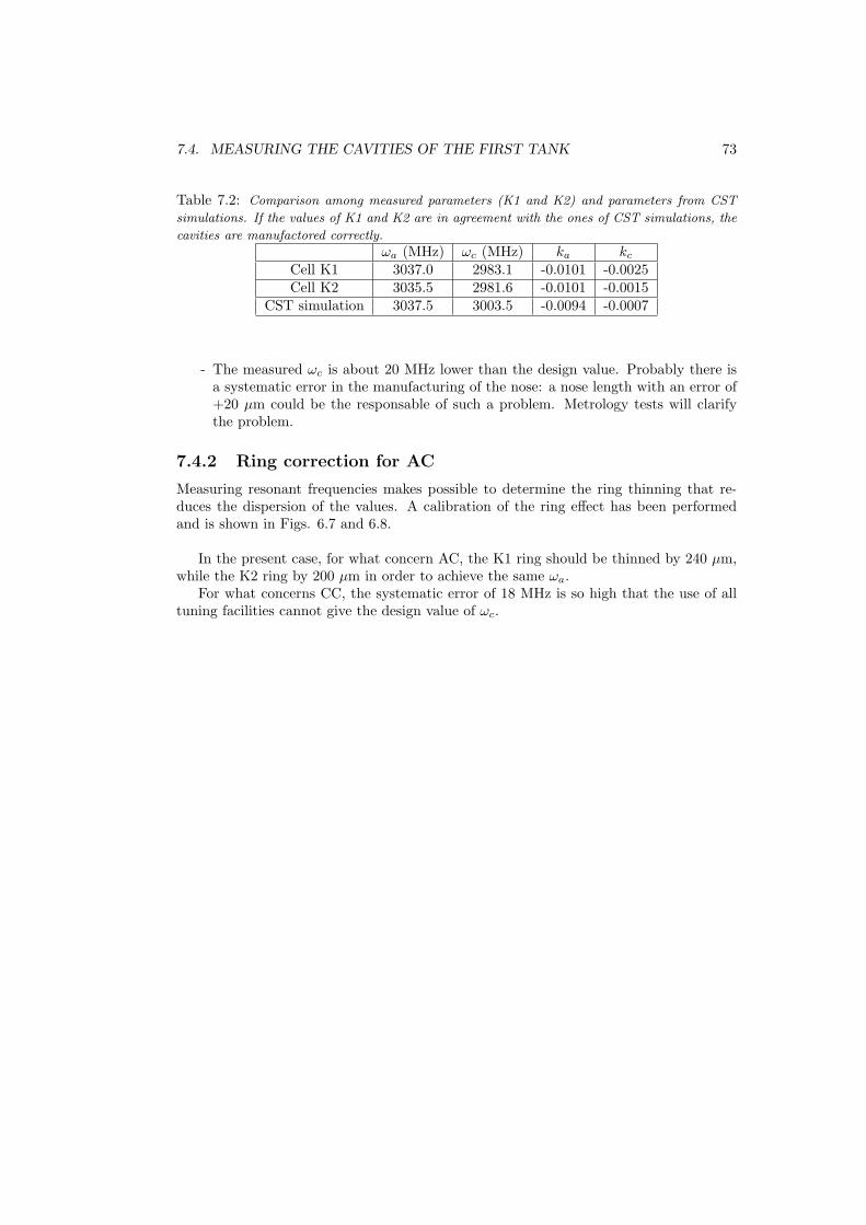
7.4. MEASURING THE CAVITIES OF THE FIRST TANK 73
Table 7.2: Comparison among measured parameters (K1 and K2) and parameters from CST
simulations. If the values of K1 and K2 are in agreement with the ones of CST simulations, the
cavities are manufactored correctly.
ωa (MHz) ωc (MHz) ka kc
Cell K1 3037.0 2983.1 -0.0101 -0.0025Cell K2 3035.5 2981.6 -0.0101 -0.0015
CST simulation 3037.5 3003.5 -0.0094 -0.0007
- The measured ωc is about 20 MHz lower than the design value. Probably there isa systematic error in the manufacturing of the nose: a nose length with an error of+20 µm could be the responsable of such a problem. Metrology tests will clarifythe problem.
7.4.2 Ring correction for AC
Measuring resonant frequencies makes possible to determine the ring thinning that re-duces the dispersion of the values. A calibration of the ring effect has been performedand is shown in Figs. 6.7 and 6.8.
In the present case, for what concern AC, the K1 ring should be thinned by 240 µm,while the K2 ring by 200 µm in order to achieve the same ωa.
For what concerns CC, the systematic error of 18 MHz is so high that the use of alltuning facilities cannot give the design value of ωc.

74 CHAPTER 7. MEASUREMENTS OF THE TANK PARAMETERS

Chapter 8
Bridge coupler
8.1 Introduction
8.1.1 Functional and mechanical overview
Figure 8.1: A LIGHT module: two tanks connected by a BC. The WG is connected to the
BAC through the coupling iris. A focusing permanent quadrupole (PMQ) is located under the
BC. This innovative feature of LIGHT makes the alignment procedure easier, because the PMQ
support system is independent of the BC.
A module, shown in Fig. 8.1, is made of two tanks connected by a bridge coupler (BC).
BC has two functions:
- joints two tanks in a unique coupled resonant structure,
- provides the coupling between the module and the waveguide (WG) for injectingthe RF power.
75

76 CHAPTER 8. BRIDGE COUPLER
It has a structure completely different from the one of the tanks: it consists of twohalf coupling cavities - named BCC, Bridge Coupling Cavities - and one central cavity -named BAC, because it’s in the position of the AC of tanks.
The magnetic couplings between the BAC and the BCCs are provided by two pairsof two semicircular slots cut in the septum between them.
Figure 8.2: The Figure shows two half BCC and one BAC, connected to the WG through the
iris (left). The definitions of the coupling coefficient of first and second order are given (right).
The coupling constants are (see Fig. 8.2 right): kba−bc and kbc−ac (first order); kba−ac
(second order for BAC and AC); kbc−cc and kbc−bc (second order for BCC). As shown inFig. 8.2 (left), the pairs of slots are rotated by 90 deg, in order to minimize the secondorder coupling for a given kba−bc.
BAC is connected to WG through the transversal iris shown in Fig. 8.2 (left).
The BC design has two main goals :
- to tune BAC and BCC to ωa and ωc respectively, in order to preserve the biperiodicinfinite chain structure in the module. A mistuning would force a different config-uration of the Eigenvectors of the system (Eq. 3.22) and a non uniformity of the Efields in the cavities;
- to provide the right coupling between BAC and WG, so to minimize the powerreflected into WG. The optimum is obtained when all the power flows through theiris from WG to BAC.
These two goals are strongly correlated, because the dimensions of the iris, the BACresonant frequency ωba, the BCC resonant frequency ωbc and the first and the secondorder coupling costants influence each other. Therefore, the design is an iterative processduring which the parameters are obtained and then refined at each step.

8.2. DRAFT DESIGN 77
8.1.2 Working rationale
Since the BC introduces a discontinuity in the periodic structure of Fig. 8.1, the analyticalmethods developed in Chapter 5 for tank design are not appropriate, because they arebased on the preservation of the infinite chain symmetry.
This consideration makes the BC design a challanging task that cannot be faced withan analytical and safe procedure. The experience of the designer is a fundamental ingre-dient, since he/she has to take several educated guesses to obtain the final parameters.
These difficulties oblige to introduce important tuning devices in the BC cavities. Thefinal tuning is performed only when the BC is inserted between the two tanks before thefinal brazing.
The purpose of this Chapter is to give a set of considerations that, although not al-ways fully justified, are useful as a starting point for the final design.
The arguments are presented in this Sections.
1. Draft design (see Section 8.2). As starting point a previous design of the BC hasbeen used. The accuracy of its resonant frequencies was about ±150 MHz.
A draft design of BC is obtained under the hypothesis of the infinite chain structure.An educated guess on the possible precision of cavities parameters that can beobtained with this method and an estimation of kba−bc for different coupling slotdimensions are made in Sections 8.2.1 and 8.2.3 respectively. The accuracy of thisdesign is expected to be about ±10 MHz.
2. Power supply (Section 8.3). The first part (see Section 8.3.1) contains the theoreticalmodel describing the matching between WG and a resonant structure. Then it isexplained how to calculate the matching parameters by means of 3D simulations.This method is tested on a pillbox cavity (Section 8.3.2). In Section 8.3.4 it isapplied to the BC and the possibility to obtain useful results for the whole moduleis highlighted.
The final Section 8.3.5 is a validation of the precision of the 3D simulations obtainedby comparing their results with the theoretical model of Section 8.3.1. This controlis necessary before performing the complete simulations for the final design to obtainthe correct matching parameters.
3. Final design procedure (Section 8.4). The aim of this part is to suggest a newmethod to calculate BC cavities parameters. It should overcome the limits of themethod used for the draft design (in Section 8.2) because BC is not considered aninfinite periodic structure.
At the moment the outcome is the result of an experience-driven estimation and nosystematic approach to evaluate the accuracy of this method has been developed.
8.2 Draft design
A previous BC design was used as a starting point. Its rough precision (frequency errorsof about ±150 MHz) was due to the fact that the study was based on 2D simulationsonly.
In the first step of this new procedure, the BC is considered part of a periodic structure(see Fig. 8.3) so that the methods outlined for tank design in Chapters 6 and 7 can beused.

78 CHAPTER 8. BRIDGE COUPLER
Figure 8.3: Two BC joined together to build up a 5 cavities structure. This configuration is used
for CST-Microwave simulations in order to obtain parameters for a draft design.
In the following CST simulations, two BCs were combined together in order to havefive coupled cavities and to apply the five parameters method of Sec. 5.2.2.
8.2.1 Validity limits of the approximation
Of course, the geometry of Fig. 8.3 does not reproduce faithfully the BC as it is in itsfinal position between the two tanks (see Fig. 8.1). Thus the parameters obtained in thisway will be affected by errors induced by the incorrect symmetry of the structure. Thefollowing considerations are important to understand the limits of this model:
- ωBAC should be fairly precise, because its final geometry (see Fig. 8.1) is exactlyreproduced in the five cavities structure of Fig. 8.3. A few 3D simulations induceto estimate an accuracy of about 10 MHz;
- in the final structure of Fig. 8.1, half BCC is combined with the half CC of thetank to make a single coupling cavity. Therefore, since geometry of Fig. 8.3 doesnot consider this effect, ωBCC calculation should be less precise than the one forωBAC . An accuracy of about 20 MHz is a reasonable guess;
- the first order coupling parameter kba−bc depends on the slot geometry and on themagnetic field intensity in the middle of the slot (see Eq. 3.12). In the approxima-tion of Fig. 8.3 the geometry is correct with respect to the one of Fig. 8.1, but themagnetic field intensity could be different due to the incorrect symmetry boundaryconditions. Therefore kba−bc is thought to be correct within a 15% error.
- kba−ba and kbc−bc, the second order coupling parameters of the approximate struc-ture (see Fig. 8.3), have no relation with the ones of the final module (see Fig. 8.1)and are useless for its design.
These considerations are result of experience-driven deduction rather than mathemat-ical proofs, but they are still useful for a draft study.
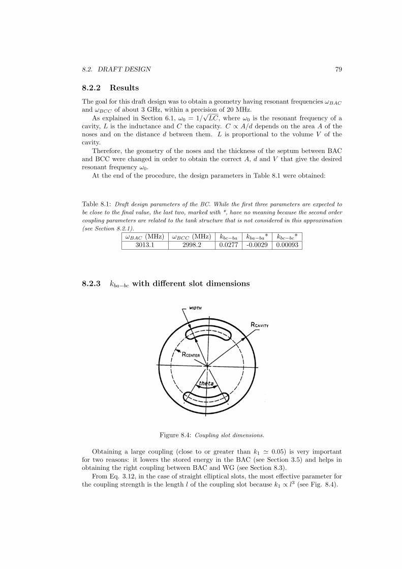
8.2. DRAFT DESIGN 79
8.2.2 Results
The goal for this draft design was to obtain a geometry having resonant frequencies ωBAC
and ωBCC of about 3 GHz, within a precision of 20 MHz.As explained in Section 6.1, ω0 = 1/
√LC, where ω0 is the resonant frequency of a
cavity, L is the inductance and C the capacity. C ∝ A/d depends on the area A of thenoses and on the distance d between them. L is proportional to the volume V of thecavity.
Therefore, the geometry of the noses and the thickness of the septum between BACand BCC were changed in order to obtain the correct A, d and V that give the desiredresonant frequency ω0.
At the end of the procedure, the design parameters in Table 8.1 were obtained:
Table 8.1: Draft design parameters of the BC. While the first three parameters are expected to
be close to the final value, the last two, marked with *, have no meaning because the second order
coupling parameters are related to the tank structure that is not considered in this approximation
(see Section 8.2.1).
ωBAC (MHz) ωBCC (MHz) kbc−ba kba−ba* kbc−bc*3013.1 2998.2 0.0277 -0.0029 0.00093
8.2.3 kba−bc with different slot dimensions
Figure 8.4: Coupling slot dimensions.
Obtaining a large coupling (close to or greater than k1 ' 0.05) is very importantfor two reasons: it lowers the stored energy in the BAC (see Section 3.5) and helps inobtaining the right coupling between BAC and WG (see Section 8.3).
From Eq. 3.12, in the case of straight elliptical slots, the most effective parameter forthe coupling strength is the length l of the coupling slot because k1 ∝ l3 (see Fig. 8.4).
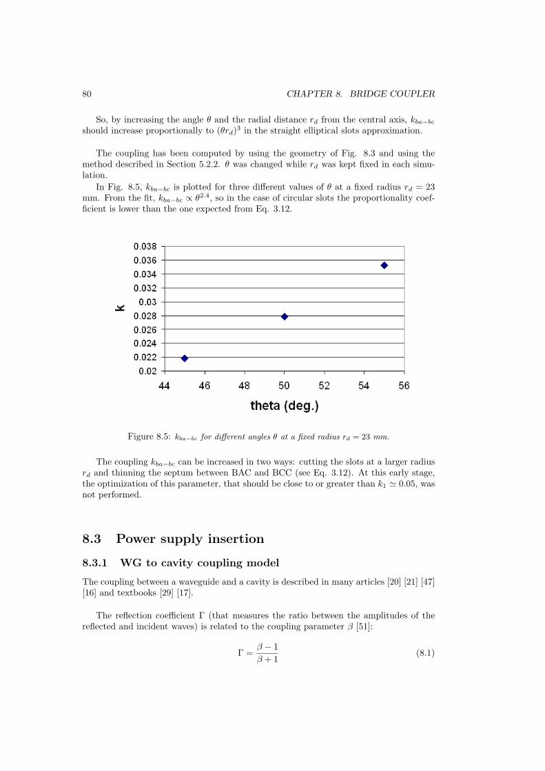
80 CHAPTER 8. BRIDGE COUPLER
So, by increasing the angle θ and the radial distance rd from the central axis, kba−bc
should increase proportionally to (θrd)3 in the straight elliptical slots approximation.
The coupling has been computed by using the geometry of Fig. 8.3 and using themethod described in Section 5.2.2. θ was changed while rd was kept fixed in each simu-lation.
In Fig. 8.5, kba−bc is plotted for three different values of θ at a fixed radius rd = 23mm. From the fit, kba−bc ∝ θ2.4, so in the case of circular slots the proportionality coef-ficient is lower than the one expected from Eq. 3.12.
Figure 8.5: kba−bc for different angles θ at a fixed radius rd = 23 mm.
The coupling kba−bc can be increased in two ways: cutting the slots at a larger radiusrd and thinning the septum between BAC and BCC (see Eq. 3.12). At this early stage,the optimization of this parameter, that should be close to or greater than k1 ' 0.05, wasnot performed.
8.3 Power supply insertion
8.3.1 WG to cavity coupling model
The coupling between a waveguide and a cavity is described in many articles [20] [21] [47][16] and textbooks [29] [17].
The reflection coefficient Γ (that measures the ratio between the amplitudes of thereflected and incident waves) is related to the coupling parameter β [51]:
Γ =β − 1β + 1
(8.1)
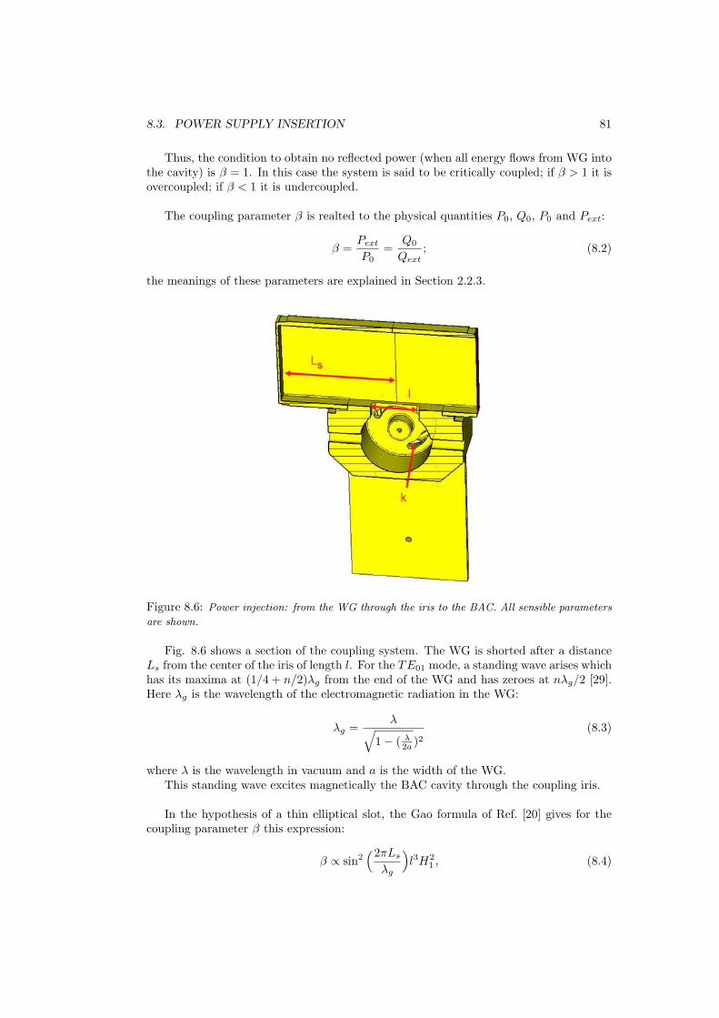
8.3. POWER SUPPLY INSERTION 81
Thus, the condition to obtain no reflected power (when all energy flows from WG intothe cavity) is β = 1. In this case the system is said to be critically coupled; if β > 1 it isovercoupled; if β < 1 it is undercoupled.
The coupling parameter β is realted to the physical quantities P0, Q0, P0 and Pext:
β =Pext
P0=
Q0
Qext; (8.2)
the meanings of these parameters are explained in Section 2.2.3.
Figure 8.6: Power injection: from the WG through the iris to the BAC. All sensible parameters
are shown.
Fig. 8.6 shows a section of the coupling system. The WG is shorted after a distanceLs from the center of the iris of length l. For the TE01 mode, a standing wave arises whichhas its maxima at (1/4 + n/2)λg from the end of the WG and has zeroes at nλg/2 [29].Here λg is the wavelength of the electromagnetic radiation in the WG:
λg =λ√
1− ( λ2a )2
(8.3)
where λ is the wavelength in vacuum and a is the width of the WG.This standing wave excites magnetically the BAC cavity through the coupling iris.
In the hypothesis of a thin elliptical slot, the Gao formula of Ref. [20] gives for thecoupling parameter β this expression:
β ∝ sin2(2πLs
λg
)l3H2
1 , (8.4)

82 CHAPTER 8. BRIDGE COUPLER
where l is the iris length and H1 is the magnetic field in the middle of the iris. As ex-pected, the maximum β is obtained when the iris is cut in correspondence to a maximumof the standing wave (for n = 1, Ls = 3λg/4).
Since Q0 is a parameter of the module determined only by the geometry of the cavities,in this case Q0 ' 5300 (see Section 6.7), to satisfy at the same time equation 8.2 and 8.4,Qext has to be proportional to
1Qext
∝ sin2(2πLs
λg
)l3H2
1 (8.5)
In this work, since Q0 is a known fix parameter, it has been decided to find the desiredvalue Qext = Q0, by adjusting the parameters Ls, l and H1. Actually, while Ls and l aregeometric parameters, H1 is related to kba−bc (the coupling between BAC and BCC): ifkba−bc increases, H1 decreases (see Section 3.5) and so does β.
Moreover, the parameter Ls can be adjusted after the brazing by using a special end-cap for the WG. Therefore Qext varies between its minimum, for Ls = 3λg/4, and +∞,for Ls = λg/2. This consideration suggests to start from Qext < 5000 and then to reachthe desired value by adjusting Ls.
Qext has to be precisely calculated with 3D simulations.
8.3.2 Calculating Qext by CST-Microwave simulations
In Ref. [40] two ways to measure QL are described.
1. In a free running cavity, when the external excitation is over, the stored energy Wdecreases exponentially (see Section 2.2.3)
W = W0e−t/τw τw =
QL
ω0(8.6)
and QL can be calculated by fitting the W (t) curve.
2. While an external excitation is applied, cavities have a resonant peak centered inω0, the resonant frequency of the desired mode. The QL of the cavity is defined by
QL =ω0
∆ωH(8.7)
where ∆ωH is the full width at half maximum of the resonant peak. In Ref. [40]it is proven that this method is successful only if the excitation is on. If ∆ωH ismeasured when the excitation is over - during the exponential decay of the storedenergy - Eq. 8.7 is not correct.
Before studying the BC, these methods were tested with a pillbox cavity fed by arectangular WG through an iris similar to the one that feeds the module.
As discussed in Section 5.1.2, to perform these calculation CST has to be used withthe time domain solver. The user decides the width of a square pulse in the frequencydomain -centered on the desired frequency- and the position of the excitation port (seeFig. 8.7 top). The solver anti-transforms the excitation in the time domain (see Fig. 8.7
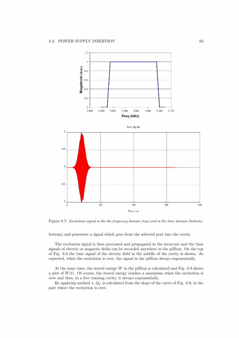
8.3. POWER SUPPLY INSERTION 83
Figure 8.7: Excitation signal in the the frequency domain (top) and in the time domain (bottom).
bottom) and generates a signal which goes from the selected port into the cavity.
The excitation signal is then processed and propagated in the structure and the timesignals of electric or magnetic fields can be recorded anywhere in the pillbox. On the topof Fig. 8.8 the time signal of the electric field in the middle of the cavity is shown. Asexpected, when the excitation is over, the signal in the pillbox decays exponentially.
At the same time, the stored energy W in the pillbox is calculated and Fig. 8.9 showsa plot of W (t). Of course, the stored energy reaches a maximum when the excitation isover and then, in a free running cavity, it decays exponentially.
By applying method 1, QL is calculated from the slope of the curve of Fig. 8.9, in thepart where the excitation is over.
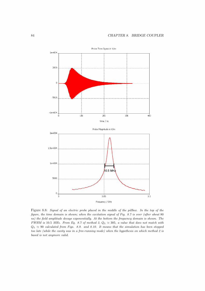
84 CHAPTER 8. BRIDGE COUPLER
Figure 8.8: Signal of an electric probe placed in the middle of the pillbox. In the top of the
figure, the time domain is shown; when the excitation signal of Fig. 8.7 is over (after about 80
ns) the field amplitude decays exponentially. At the bottom the frequency domain is shown. The
FWHM is 10.5 MHz. From Eq. 8.7 of method 2, QL ' 305, a value that does not match with
QL ' 90 calculated from Figs. 8.9. and 8.10. It means that the simulation has been stopped
too late (while the cavity was in a free-running mode) when the hypothesis on which method 2 is
based is not anymore valid.
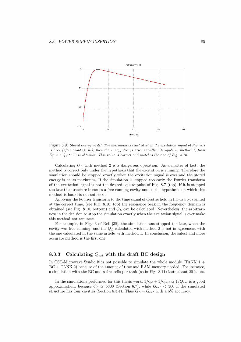
8.3. POWER SUPPLY INSERTION 85
Figure 8.9: Stored energy in dB. The maximum is reached when the excitation signal of Fig. 8.7
is over (after about 80 ns); then the energy decays exponentially. By applying method 1, from
Eq. 8.6 QL ' 90 is obtained. This value is correct and matches the one of Fig. 8.10.
Calculating QL with method 2 is a dangerous operation. As a matter of fact, themethod is correct only under the hypothesis that the excitation is running. Therefore thesimulation should be stopped exactly when the excitation signal is over and the storedenergy is at its maximum. If the simulation is stopped too early the Fourier transformof the excitation signal is not the desired square pulse of Fig. 8.7 (top); if it is stoppedtoo late the structure becomes a free running cavity and so the hypothesis on which thismethod is based is not satisfied.
Applying the Fourier transform to the time signal of electric field in the cavity, stuntedat the correct time, (see Fig. 8.10, top) the resonance peak in the frequency domain isobtained (see Fig. 8.10, bottom) and QL can be calculated. Nevertheless, the arbitrari-ness in the decision to stop the simulation exactly when the excitation signal is over makethis method not accurate.
For example, in Fig. 3 of Ref. [35], the simulation was stopped too late, when thecavity was free-running, and the QL calculated with method 2 is not in agreement withthe one calculated in the same article with method 1. In conclusion, the safest and moreaccurate method is the first one.
8.3.3 Calculating Qext with the draft BC design
In CST-Microwave Studio it is not possible to simulate the whole module (TANK 1 +BC + TANK 2) because of the amount of time and RAM memory needed. For instance,a simulation with the BC and a few cells per tank (as in Fig. 8.11) lasts about 20 hours.
In the simulations performed for this thesis work, 1/Q0 + 1/Qext ' 1/Qext is a goodapproximation, because Q0 ' 5300 (Section 6.7), while Qext < 300 if the simulatedstructure has four cavities (Section 8.3.4). Thus QL = Qext with a 5% accuracy.
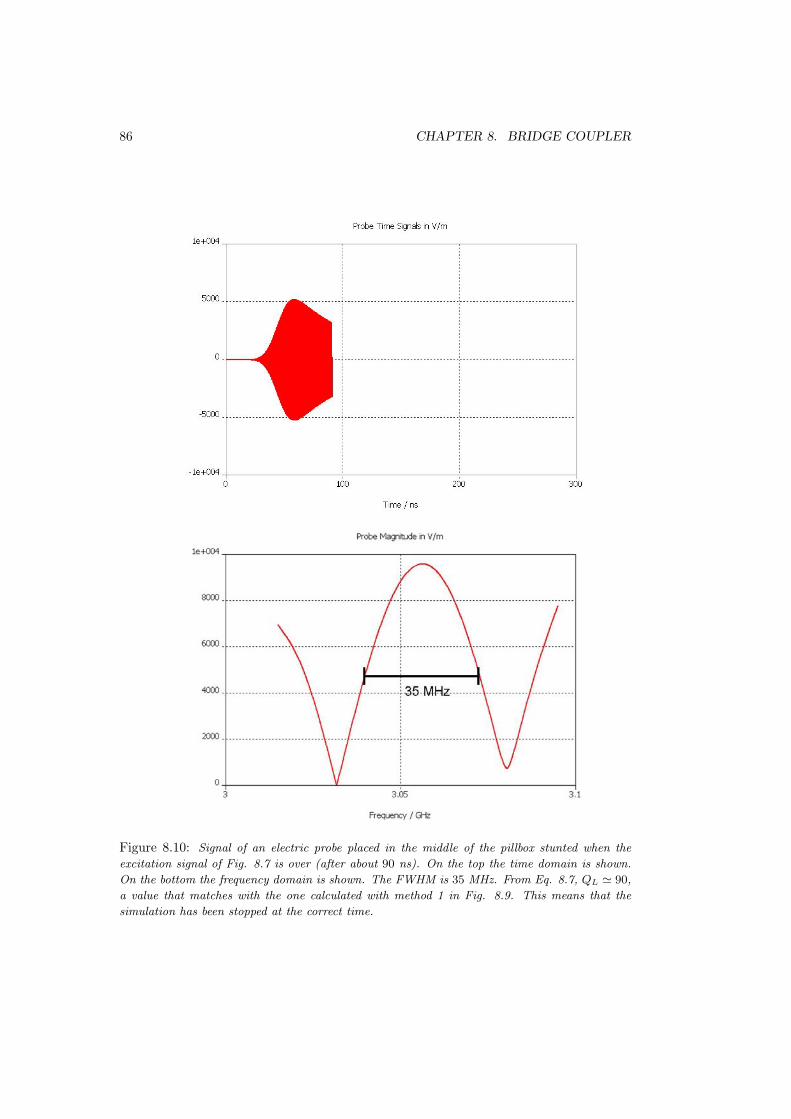
86 CHAPTER 8. BRIDGE COUPLER
Figure 8.10: Signal of an electric probe placed in the middle of the pillbox stunted when the
excitation signal of Fig. 8.7 is over (after about 90 ns). On the top the time domain is shown.
On the bottom the frequency domain is shown. The FWHM is 35 MHz. From Eq. 8.7, QL ' 90,
a value that matches with the one calculated with method 1 in Fig. 8.9. This means that the
simulation has been stopped at the correct time.
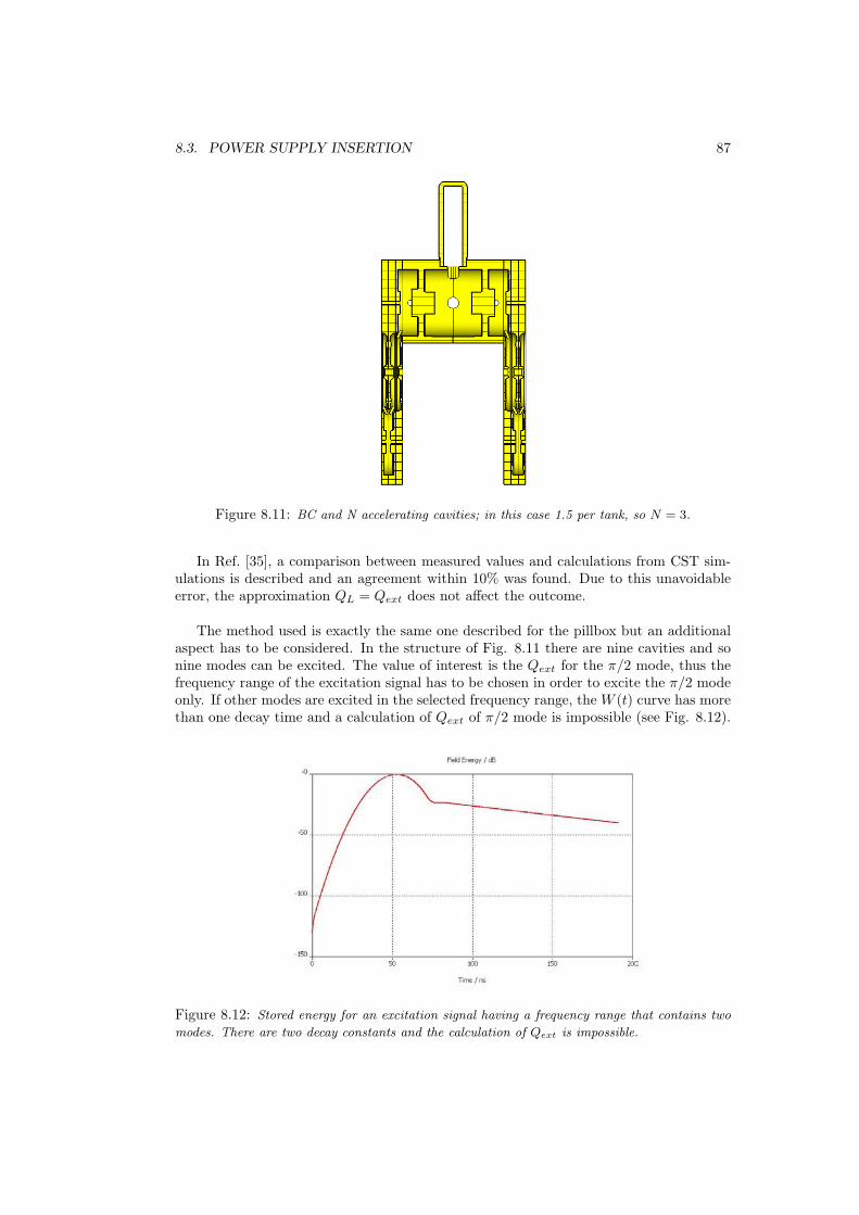
8.3. POWER SUPPLY INSERTION 87
Figure 8.11: BC and N accelerating cavities; in this case 1.5 per tank, so N = 3.
In Ref. [35], a comparison between measured values and calculations from CST sim-ulations is described and an agreement within 10% was found. Due to this unavoidableerror, the approximation QL = Qext does not affect the outcome.
The method used is exactly the same one described for the pillbox but an additionalaspect has to be considered. In the structure of Fig. 8.11 there are nine cavities and sonine modes can be excited. The value of interest is the Qext for the π/2 mode, thus thefrequency range of the excitation signal has to be chosen in order to excite the π/2 modeonly. If other modes are excited in the selected frequency range, the W (t) curve has morethan one decay time and a calculation of Qext of π/2 mode is impossible (see Fig. 8.12).
Figure 8.12: Stored energy for an excitation signal having a frequency range that contains two
modes. There are two decay constants and the calculation of Qext is impossible.
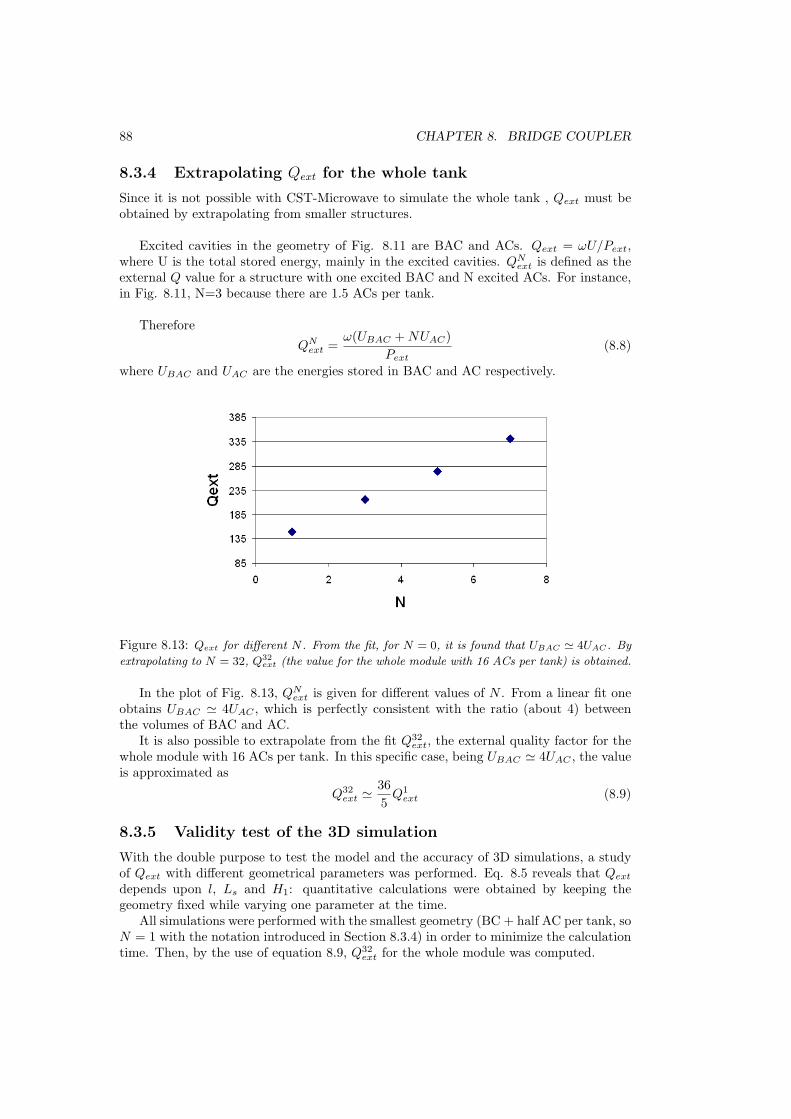
88 CHAPTER 8. BRIDGE COUPLER
8.3.4 Extrapolating Qext for the whole tank
Since it is not possible with CST-Microwave to simulate the whole tank , Qext must beobtained by extrapolating from smaller structures.
Excited cavities in the geometry of Fig. 8.11 are BAC and ACs. Qext = ωU/Pext,where U is the total stored energy, mainly in the excited cavities. QN
ext is defined as theexternal Q value for a structure with one excited BAC and N excited ACs. For instance,in Fig. 8.11, N=3 because there are 1.5 ACs per tank.
Therefore
QNext =
ω(UBAC + NUAC)Pext
(8.8)
where UBAC and UAC are the energies stored in BAC and AC respectively.
Figure 8.13: Qext for different N . From the fit, for N = 0, it is found that UBAC ' 4UAC . By
extrapolating to N = 32, Q32ext (the value for the whole module with 16 ACs per tank) is obtained.
In the plot of Fig. 8.13, QNext is given for different values of N . From a linear fit one
obtains UBAC ' 4UAC , which is perfectly consistent with the ratio (about 4) betweenthe volumes of BAC and AC.
It is also possible to extrapolate from the fit Q32ext, the external quality factor for the
whole module with 16 ACs per tank. In this specific case, being UBAC ' 4UAC , the valueis approximated as
Q32ext '
365
Q1ext (8.9)
8.3.5 Validity test of the 3D simulation
With the double purpose to test the model and the accuracy of 3D simulations, a studyof Qext with different geometrical parameters was performed. Eq. 8.5 reveals that Qext
depends upon l, Ls and H1: quantitative calculations were obtained by keeping thegeometry fixed while varying one parameter at the time.
All simulations were performed with the smallest geometry (BC + half AC per tank, soN = 1 with the notation introduced in Section 8.3.4) in order to minimize the calculationtime. Then, by the use of equation 8.9, Q32
ext for the whole module was computed.
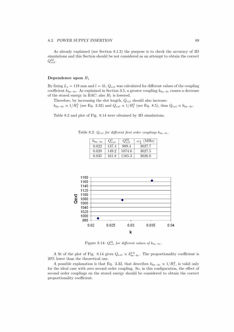
8.3. POWER SUPPLY INSERTION 89
As already explained (see Section 8.1.2) the purpose is to check the accuracy of 3Dsimulations and this Section should be not considered as an attempt to obtain the correctQ32
ext.
Dependence upon H1
By fixing Ls = 118 mm and l = 41, Qext was calculated for different values of the couplingcoefficient kba−bc. As explained in Section 3.5, a greater coupling kba−bc causes a decreaseof the stored energy in BAC: also H1 is lowered.
Therefore, by increasing the slot length, Qext should also increase:kba−bc ∝ 1/H2
1 (see Eq. 3.32) and Qext ∝ 1/H21 (see Eq. 8.5), thus Qext ∝ kba−bc.
Table 8.2 and plot of Fig. 8.14 were obtained by 3D simulations.
Table 8.2: Qext for different first order couplings kba−bc.
kba−bc Q1ext Q32
ext ωπ2
(MHz)0.022 137.4 989.4 3027.70.028 149.2 1074.6 3027.50.035 161.8 1165.3 3026.0
Figure 8.14: Q32ext for different values of kba−bc.
A fit of the plot of Fig. 8.14 gives Qext ∝ k0.8ba−bc. The proportionality coefficient is
20% lower than the theoretical one.A possible explanation is that Eq. 3.32, that describes kba−bc ∝ 1/H2
1 , is valid onlyfor the ideal case with zero second order coupling. So, in this configuration, the effect ofsecond order couplings on the stored energy should be considered to obtain the correctproportionality coefficient.
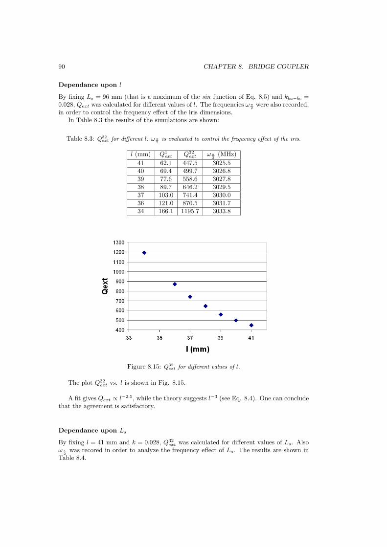
90 CHAPTER 8. BRIDGE COUPLER
Dependance upon l
By fixing Ls = 96 mm (that is a maximum of the sin function of Eq. 8.5) and kba−bc =0.028, Qext was calculated for different values of l. The frequencies ωπ
2were also recorded,
in order to control the frequency effect of the iris dimensions.In Table 8.3 the results of the simulations are shown:
Table 8.3: Q32ext for different l. ω π
2is evaluated to control the frequency effect of the iris.
l (mm) Q1ext Q32
ext ωπ2
(MHz)41 62.1 447.5 3025.540 69.4 499.7 3026.839 77.6 558.6 3027.838 89.7 646.2 3029.537 103.0 741.4 3030.036 121.0 870.5 3031.734 166.1 1195.7 3033.8
Figure 8.15: Q32ext for different values of l.
The plot Q32ext vs. l is shown in Fig. 8.15.
A fit gives Qext ∝ l−2.5, while the theory suggests l−3 (see Eq. 8.4). One can concludethat the agreement is satisfactory.
Dependance upon Ls
By fixing l = 41 mm and k = 0.028, Q32ext was calculated for different values of Ls. Also
ωπ2
was recored in order to analyze the frequency effect of Ls. The results are shown inTable 8.4.
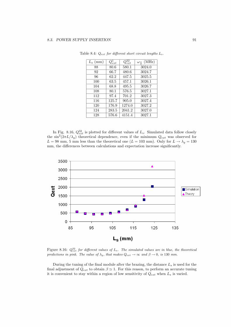
8.3. POWER SUPPLY INSERTION 91
Table 8.4: Qext for different short circuit lengths Ls.
Ls (mm) Q1ext Q32
ext ωπ2
(MHz)88 80.6 580.1 3024.092 66.7 480.6 3024.796 62.2 447.5 3025.5100 63.5 457.1 3026.1104 68.8 495.5 3026.7108 80.1 576.5 3027.1112 97.4 701.2 3027.3116 125.7 905.0 3027.4120 176.9 1274.0 3027.2124 283.5 2041.2 3027.0128 576.6 4151.4 3027.1
In Fig. 8.16, Q32ext is plotted for different values of Ls. Simulated data follow closely
the sin2(2πL/λg) theoretical dependence, even if the minimum Qext was observed forL = 98 mm, 5 mm less than the theoretical one (L = 103 mm). Only for L → λg = 130mm, the differences between calculations and expectation increase significantly.
Figure 8.16: Q32ext for different values of Ls. The simulated values are in blue, the theoretical
predictions in pink. The value of λg, that makes Qext →∞ and β → 0, is 130 mm.
During the tuning of the final module after the brazing, the distance Ls is used for thefinal adjustment of Qext to obtain β ' 1. For this reason, to perform an accurate tuningit is convenient to stay within a region of low sensitivity of Qext when Ls is varied.

92 CHAPTER 8. BRIDGE COUPLER
Final considerations
The comparison between CST simulations and theoretical values described in this Sectionvalidates the accuracy of the simulations. Indeed agreements of about 10% have beenfound.
This outcome is extremely important because the design of the coupling iris of theLIBO 4th unit was made according to theoretical calculations only. This new methodguarantees a better precision and an easier matching to the WG during the final tuningphase.
Before the beginning of the final design, kba−ba has to be raised at least up to 0.05(the value of k1 in the tanks).
As explained in Section 8.3.1, to obtain β ' 1, Q32ext should be equal to Q0 = 5000.
Therefore the iris length l has to be chosen to have the desired value of Q32ext.
8.4 Final design procedure
To obtain the final design, all the BC parameters (resonant frequencies and coupling val-ues) have to be calculated with an accuracy of about 5 MHz and 5% respectively. Thisprecision cannot be obtained with the method based on the infinite chain symmetry de-scribed in Section 8.2. A new method is being developed to satisfy the requested precision.
Figure 8.17: Configuration used to measure resonant frequencies and coupling parameters. All
cavities are shorted but the triplet of interest, in this case AC-BCC-BAC. The parameters are
then calculated with methods similar to those described in Section 7.2.
The main idea is the introduction of copper pieces in the holes to short circuit all thecavities but the triplet of interest (see Fig. 8.17). A method similar to those describedin Section 7.2 will be soon developed to calculate cavities parameters.

8.4. FINAL DESIGN PROCEDURE 93
With respect to Section 7.2, the boundary conditions are different because the tripletsare terminated with full cells and so there are not reflection and symmetry breaking effects.
Geometries with triplets formed by CC-AC-BCC, AC-BCC-BAC and BCC-BAC-BCCwill be considered and all the parameters (resonant frequencies ωBAC and ωBCC ; firstorder coupling kba−bc and kbc−ac; second order coupling kba−ac, kbc−cc and kbc−bc) willbe calculated. This procedure is time consuming but necessary to obtain a good design.
This method should guarantee the requested precision of 5 MHz on the resonant fre-quencies and of 5% on the coupling parameters. This statement is a result of experience-driven considerations and it has not been yet systematically studied.
Of course the manufacturing of a BC prototype is forseen to verify if the assumedprecision of this design method is confirmed or not.

94 CHAPTER 8. BRIDGE COUPLER

Chapter 9
Conclusions
9.1 Achievements
The detailed study of the physics of coupled cavities brought important and novel resultswhich concern both the theoretical and the experimental aspects of the problem.
The first issue is related to the investigation of the effects of the boundary conditionsand symmetry breaking in finite chain structures (Chapter 4). This study established forthe first time that the inquiry of finite structures that preserve the infinite chain symmetryis the only way to obtain the parameters of an infinite chain of coupled cavities.
This result is extremely important because many methods normally used in the labo-ratory and proposed in literature are based on structures having the uncorrect symmetryand thus giving inaccurate results.
For the first time, this study explained the well known effect of the decrease of the π/2mode frequency with the increase of the number of cavities in SCL (Side Coupled Linac)chains with half accelerating cells terminations. In Section 4.2 it was introduced a modelwhich is based on the consideration that, due to symmetry breaking, the two boundarycavities have different resonant frequencies and coupling parameters with respect to themiddle ones. This model reproduces the experimental and simulated measurements withvery high accuracy (in Section 4.2).
These theoretical studies enabled the development of a very accurate procedure to ob-tain the cavities parameters. The method exploits a five cavities chain with half couplingcells terminations that preserve the symmetry of the infinite chain. By inserting the fiveresonant frequencies in a five equations system, the desired parameters are obtained bysolving analitically the system (see Section 5.2).
This innovative analytical method, compared to previous iterative ones, has the rele-vant practical implication of being less time consuming and of improving the precision ofthe final parameters.
Exploiting this novel and fast method, a new algorithm was developed (see Chapter6) which is capable to perform cavities design and optimize accelerators performancesby using 3D electromagnetic field solver codes (see Chapter 6). The accuracy of the 3Dsimulations was validated by a comparison with experimental measurements.
The application of this rationale made possible the design and the optimization of the
95

96 CHAPTER 9. CONCLUSIONS
first module and a study of the resonant frequency effects of the mechanical tolerancesrequested to the producers.
To check the accuracy of the manufactoring, cavities parameters need to be carefullymeasured. Therefore a precise experimental method was conceived taking into accountall the considerations made on symmetries of the chain boundaries (see Chapter 7).
New technical solutions were studied to avoid systematic errors and then successfullytested by a comparison between measurements and simulations.
This method was applied to a couple of test cavities of tank 1, manufactured accord-ing to the design of Chapter 6. The measurements pointed out a systematic error on theproduction of the coupling cavities.
Finally a preliminary study was performed on the bridge coupler, the item locatedbetween two accelerating tanks that receives the power needed for particle acceleration(Chapter 8).
Since this structure is aperiodic, methods developed for tank design can be appliedonly for a draft design, because they are based on the preservation of the structuresymmetry. Validity limits of this approximation were estimated and a procedure toaccomplish the final design was outlined.
A study of the power insertion from the waveguide to the bridge cavity was made andsimulated results were compared to theoretical prediction. Preliminary results suggestthat the difference is about 10%, good enough to pass to the final design.
9.2 Further studies
The first forseen application of the developed method is to accomplish the design of thetanks 3 and 4 of the First Unit.
In order to decrease the number of steps needed for the tuning, a new design withoutthe tuning ring is being studied.
Secondly, the optimization of the bridge coupler must be performed.The best resonant frequency of the central bridge cavity must be chosen in order to
maximize the electric field flatness of the whole module and the power distribution in thecavities. It would be useful to write a code that solves the matrix of the circuit model ofthe whole tank in order to compute the amplitude of the electric field in each cavity.
After this study, the final design of the bridge coupler will have to be performed bytaking into account the effects of the coupling to the waveguide.
The study of aperiodic resonant chains is really important not only for the bridgecoupler, but also for the measurements of the cavities parameters. As a matter of fact,manufactured cavities are not identical due to mechanical imperfections and thus, oncestacked together, do not form a perfect infinite chain.
This problem may require the development of new methods, based on genetic al-gorithms and neural networks. This new approach is required to face and solve thecomplexity of computing the resonant frequencies and coupling parameters of each cavitygiven the Eigenfrequencies of a finite length chain.

Appendix A
CST-MICROWAVE mesh andprecision tips
CST performance and precision is largely affected by the number of mesh cells. A standardPC with 4Gb of RAM can bear about 1.5 million mesh cells.
Usually good parameters for generating the mesh are:
• 45 lines per wavelength
• 30 lower mesh limit
With such a mesh a 9 modes minitank is simulated in about 30 m.
During the first simulations it is recommended to use the adaptive mesh tool, becauseit gives an idea of the frequency fluctuations due to different meshes. This can be helpfulin choosing a proper mesh for the following simulations.
If a comparison between two simulations is needed, it is essential that they have thesame mesh. Different meshes give results which differ even by 5 MHz.
97

98 APPENDIX A. CST-MICROWAVE MESH AND PRECISION TIPS

Appendix B
Technical guide: measuringtank parameters
This Appendix describes a technique to measure the values ωat, ωct, kat and kc which arerespectively the resonant frequency of the accelerating (AC) and the coupling (CC) cellsand the coupling parameters between AC→CC, AC→AC and CC→CC. It is written inthe style of a laboratory note to be used by skillful operators.
Fig. B.1 shows the items and the instruments ustilised in such a measurement.
99
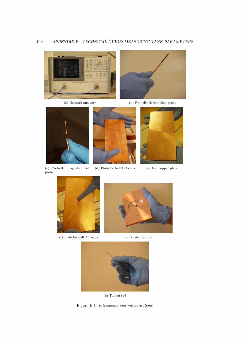
100 APPENDIX B. TECHNICAL GUIDE: MEASURING TANK PARAMETERS
(a) Network analyzer (b) ProbeE: electric field probe
(c) ProbeH: magnetic fieldprobe
(d) Plate for half CC ends (e) Full copper plate
(f) plate for half AC ends (g) Plate 1 and 2
(h) Tuning rod
Figure B.1: Intruments and measure items
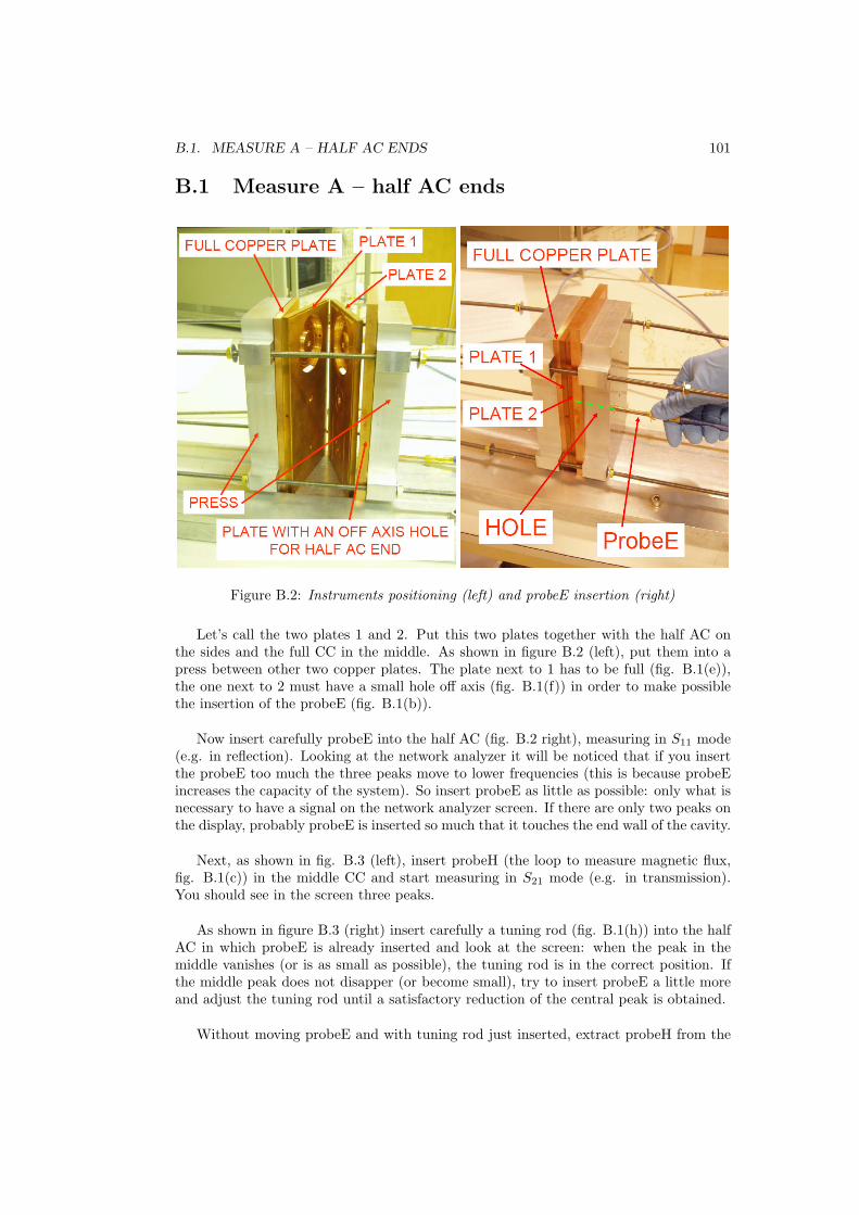
B.1. MEASURE A – HALF AC ENDS 101
B.1 Measure A – half AC ends
Figure B.2: Instruments positioning (left) and probeE insertion (right)
Let’s call the two plates 1 and 2. Put this two plates together with the half AC onthe sides and the full CC in the middle. As shown in figure B.2 (left), put them into apress between other two copper plates. The plate next to 1 has to be full (fig. B.1(e)),the one next to 2 must have a small hole off axis (fig. B.1(f)) in order to make possiblethe insertion of the probeE (fig. B.1(b)).
Now insert carefully probeE into the half AC (fig. B.2 right), measuring in S11 mode(e.g. in reflection). Looking at the network analyzer it will be noticed that if you insertthe probeE too much the three peaks move to lower frequencies (this is because probeEincreases the capacity of the system). So insert probeE as little as possible: only what isnecessary to have a signal on the network analyzer screen. If there are only two peaks onthe display, probably probeE is inserted so much that it touches the end wall of the cavity.
Next, as shown in fig. B.3 (left), insert probeH (the loop to measure magnetic flux,fig. B.1(c)) in the middle CC and start measuring in S21 mode (e.g. in transmission).You should see in the screen three peaks.
As shown in figure B.3 (right) insert carefully a tuning rod (fig. B.1(h)) into the halfAC in which probeE is already inserted and look at the screen: when the peak in themiddle vanishes (or is as small as possible), the tuning rod is in the correct position. Ifthe middle peak does not disapper (or become small), try to insert probeE a little moreand adjust the tuning rod until a satisfactory reduction of the central peak is obtained.
Without moving probeE and with tuning rod just inserted, extract probeH from the

102 APPENDIX B. TECHNICAL GUIDE: MEASURING TANK PARAMETERS
Figure B.3: ProbeH (left) and tuning rod (right) insertion into half AC
CC and work again in S11 mode (reflection), as shown in fig. B.4 (top left). Write downthe three resonant frequencies.
As shown in fig. B.4 (top right) without moving probeE and the tuning rod in thehalf AC, insert slowly a tuning rod in the full CC until the two lateral peaks shift ofa small but appreciable quantity. Write down the three new resonant frequencies (themiddle one should remain the same), move the tuning rod a little more into the cavityand write down the three frequencies again. Repeat this procedure till the tuning rodis totally inserted in the cavity. Now, leaving this tuning rod in the cavity, as shown infig. B.4 (right), insert a second tuning rod in the other hole of the CC and repeat theoperation above.
At the end you will have a list of about six measures of the triplet of frequencies. Youshould make a table marked as Plate 2→1 ending with half AC with 3 columns containingthese triplet of frequencies, as shown in section B.3.
B.2 Measure B – half CC ends
The plates should be set in the scheme of Fig. B.5 (left). The half CC ends must be inthe opposite semispace respect to the horizontal plane (one up, the other down), a fullplate must be next to plate 1 and a plate with a small off-axis hole (B.1(d)) next to plate 2.
Next insert carefully probeE through that hole into the half CC (fig. B.5 right), mea-suring in S11 mode (e.g. in reflection). Looking at the network analyzer it should be

B.2. MEASURE B – HALF CC ENDS 103
Figure B.4: Working again in reflection (left), tuning rod insertion into the full CC(center), second tuning rod insertion into the full CC (right)

104 APPENDIX B. TECHNICAL GUIDE: MEASURING TANK PARAMETERS
Figure B.5: Set up of half CC ends measurments (left), insertion of probeE into the halfCC end (right)
noticed that if you insert the probeE too much, the three peaks move to lower frequencies(this is because probeE increases the capacity of the system). So insert probeE slightly:only to have a signal on the network analyzer screen.
The measurements are the same ones described in the previous section.
As shown in fig. B.6 (left), insert probeH into the middle AC and start measuring inS21 mode (e.g. in transmission). You should see in the screen three peaks.
Next, as shown in fig. B.6 (right), insert carefully a tuning rod into the half CC inwhich probeE is already inserted and look at the screen: when the central peak vanishes(or is as small as possible), the tuning rod is in the right position. If the middle peakdoes not disapper (or become small), try to insert probeE a little more and adjust thetuning rod until the central peak behaves as above.
Without moving probeE and the tuning rod, extract probeH from the AC and workagain in S11 mode (reflection), as shown in fig. B.7 (left). Write down the three resonantfrequencies.
As shown in figure B.7 (center), without moving probeE and the tuning rod in thehalf CC, insert slowly a tuning rod in the full AC until the two lateral peaks shift ofa small but appreciable quantity. Write down the three new resonant frequencies (themiddle one should remain the same), move the tuning rod a little more into the cavityand write down the three frequencies again. Repeat this procedure till the tuning rod is

B.2. MEASURE B – HALF CC ENDS 105
Figure B.6: ProbeH is inserted in the middle AC (left), tuning rod is inserted in the halfCC end (right)
totally inserted in the cavity. Now, leaving also this tuning rod in the cavity, as shownin figure B.7 (right), insert a second tuning rod in the other hole of the AC and repeatthe operation above.
At the end you will have a list of about ten measures of the triplet of frequencies. Youshould make a table marked as Plate 2→1 ending with half CC with 3 columns containingthese triplet of frequencies as shown in section B.3.
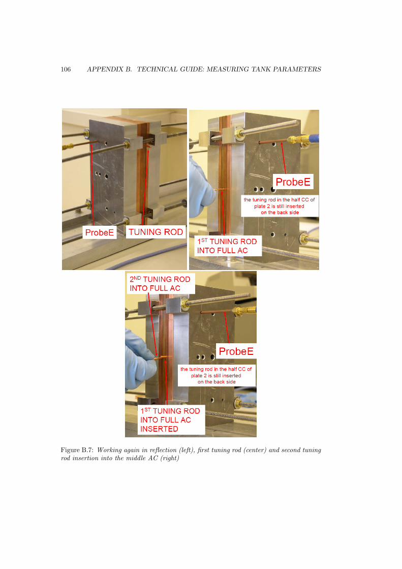
106 APPENDIX B. TECHNICAL GUIDE: MEASURING TANK PARAMETERS
Figure B.7: Working again in reflection (left), first tuning rod (center) and second tuningrod insertion into the middle AC (right)
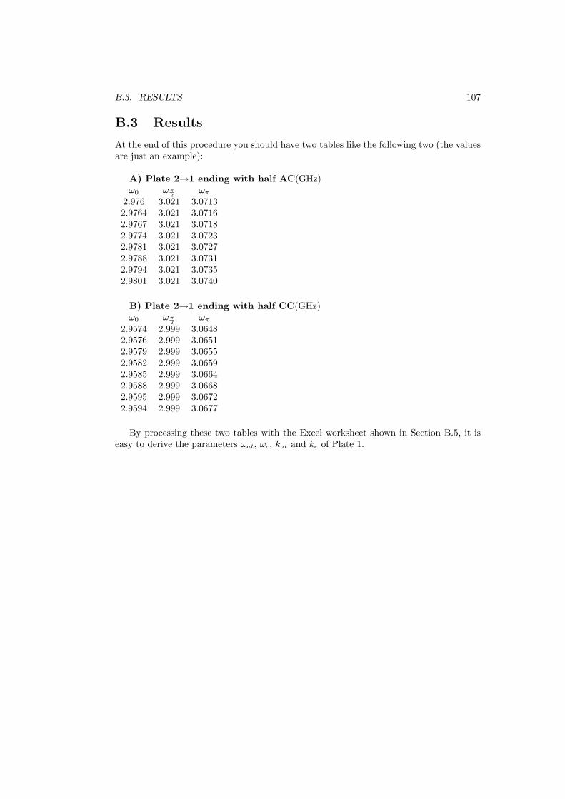
B.3. RESULTS 107
B.3 Results
At the end of this procedure you should have two tables like the following two (the valuesare just an example):
A) Plate 2→1 ending with half AC(GHz)ω0 ωπ
2ωπ
2.976 3.021 3.07132.9764 3.021 3.07162.9767 3.021 3.07182.9774 3.021 3.07232.9781 3.021 3.07272.9788 3.021 3.07312.9794 3.021 3.07352.9801 3.021 3.0740
B) Plate 2→1 ending with half CC(GHz)ω0 ωπ
2ωπ
2.9574 2.999 3.06482.9576 2.999 3.06512.9579 2.999 3.06552.9582 2.999 3.06592.9585 2.999 3.06642.9588 2.999 3.06682.9595 2.999 3.06722.9594 2.999 3.0677
By processing these two tables with the Excel worksheet shown in Section B.5, it iseasy to derive the parameters ωat, ωc, kat and kc of Plate 1.

108 APPENDIX B. TECHNICAL GUIDE: MEASURING TANK PARAMETERS
B.4 Reverse the order of the plates 1 and 2
Figure B.8: Instruments positioning
The same procedure has to be repeated by changing the position of plates 1 and 2:probeE is inserted in plate 1 and plate 2 is next to the full copper plate, as shown infigure B.8.
Two tables like those in measurements A should be filled and marked respectivelyPlate 1→2 ending with half AC and Plate 1→2 ending with half CC.
Next, by processing these two tables with the same Excel worksheet shoen in SectionB.5, it is easy to derive the parameters ωat, ωc, kat and kc of Plate 2.
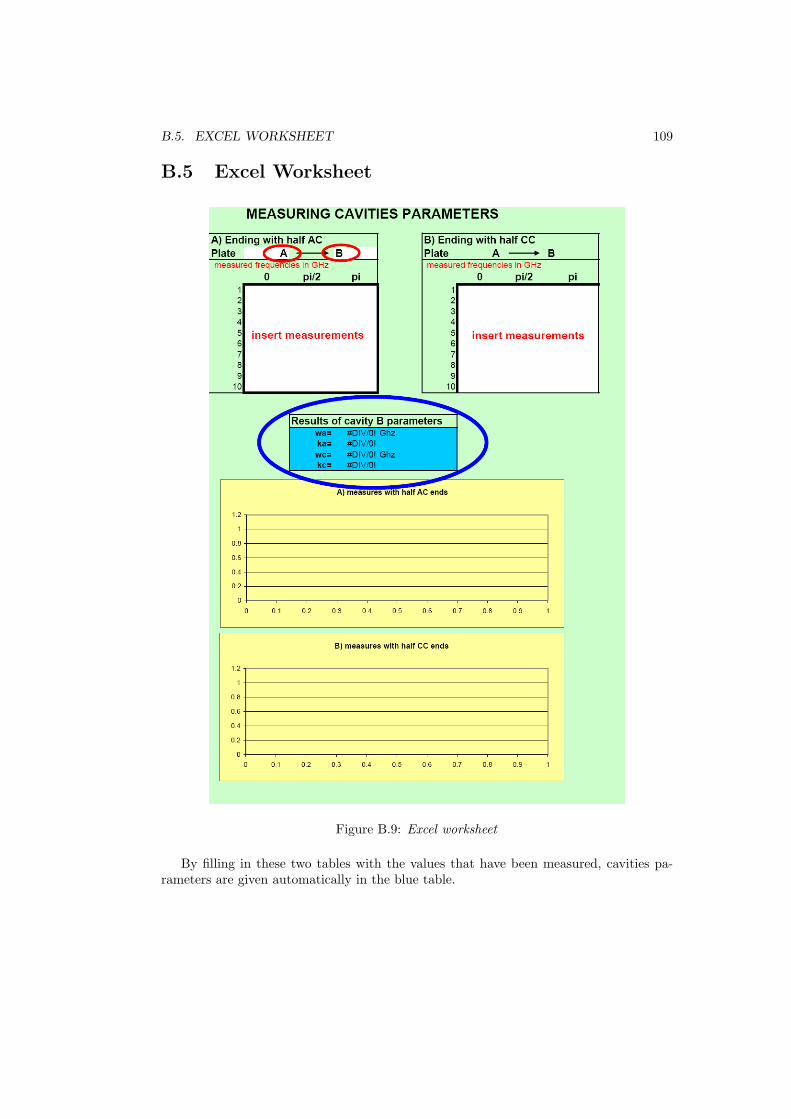
B.5. EXCEL WORKSHEET 109
B.5 Excel Worksheet
Figure B.9: Excel worksheet
By filling in these two tables with the values that have been measured, cavities pa-rameters are given automatically in the blue table.

110 APPENDIX B. TECHNICAL GUIDE: MEASURING TANK PARAMETERS
Appendix C
Scattering matrix
Considering a microwave network with N ports, the Scattering matrix contains the pa-rameters (S-parameters) that relate incoming waves to the reflected waves.
Defining an and bn as the normalized amplitude voltage of the incoming and reflectedwave on port n respectively, the S-matrix satisfies b = Sa, where
b =
b1
b2
...bN
, a =
a1
a2
...aN
, S =
S11 S12 . . . S1N
S21 S22 . . . S2N
...SN1 SN2 . . . SNN
(C.1)
In the case of our interest, a 2 × 2 matrix describes a network with two ports, forinstance an electric (port 1) and a magnetic (port 2) probe connected to a resonantcavities chain.
S11 and S22 are the reflected voltage on port 1 and 2 respectively. S12 = S21 arethe transmission coefficients, they are equal because, neglecting losses, the system issymmetric.
A network analyser excites the system with signals that span over a given frequencyrange and makes a plot of the S-parameters versus the frequency.
For example, if the system of Fig. C.1 is excited from port 1 in a range containingNp resonant frequencies, S11 shows Np negative peaks because at resonance the power isabsorbed by the cavities, while S12 has Np positive peaks because probe 2 measures theamplitude of the field in a cavity (see Fig. C.2).
111
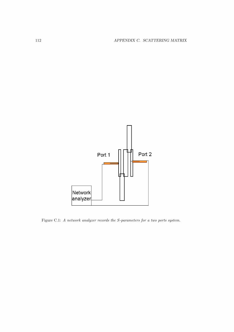
112 APPENDIX C. SCATTERING MATRIX
Figure C.1: A network analyzer records the S-parameters for a two ports system.
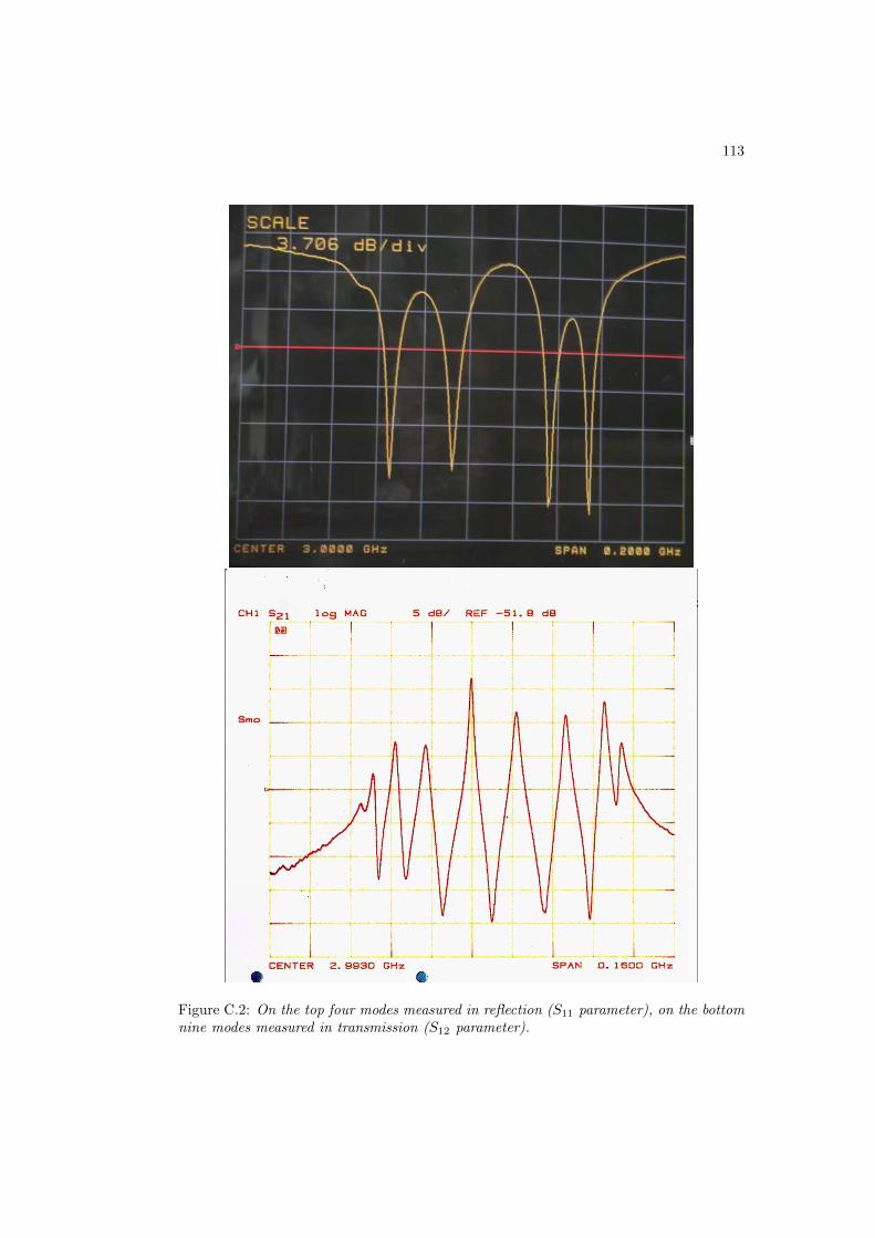
113
Figure C.2: On the top four modes measured in reflection (S11 parameter), on the bottomnine modes measured in transmission (S12 parameter).

114 APPENDIX C. SCATTERING MATRIX

Aknowledgements
In spring 2006 I was charmed by lectures on Application of Physics to Medicine given byProf. Ugo Amaldi at University Milano-Bicocca. When, in September of the same yearhe accepted me as a thesis student I was enthusiastic to work on the IDRA project.
My work at CERN started in November 2007, when I got a TERA (Fondazione per laAdroterapia Oncologica) felloship to accomplish the design of the First Unit of LIGHT,the Linac for Image Guided Hadron Therapy in the cyclinac of IDRA.
I’m really grateful to Prof. Ugo Amaldi for having given me the opportunity to studyand work in an amazing small team on such an interesting and useful project.
A special thank goes to all my closest team-mates for the wonderful atmosphere thatI breathed for one whole year. Giulio, for his unvaluable advices and his true friendshipsince the very first day. Ettore, for having taken care of me and for having supportedme in both technical and human aspects. Claudio, for the unending discussions and theunbelievable patience in making drawings for me.
I would like also to thank Alessandro D’Elia for the two long discussions we got inthe last month. He gave me the self-confidence that my studies were on the right track.
A special thank is for beloved Dr. Mario Weiss, whose imprint on the project and,particularly, on the people is still effective and sharp.
At last I cannot forget all the people I met in TERA: thank you Adriano, Paola,Giuseppe, Maria and Peter.
115

116 APPENDIX C. SCATTERING MATRIX

Bibliography
[1] U. Amaldi. Cancer therapy with particle accelerators. Nuclear Physics A,654(1):375c–399c, Jul 1999.
[2] U. Amaldi. Lectures on applications of physics to medicine, 2006.
[3] U. Amaldi. Cyclinacs: novel fast-cycling accelerators for hadrontherapy. In Interna-tional conference on cyclotrons and their applications, 2007.
[4] U. Amaldi. History of hadrontherapy in the world and italian developments. RivistaMedica, 2008.
[5] U. Amaldi and G. Kraft. Radiotherapy with beams of carbon ions. Reports onprogress in Physics, 2005.
[6] U. Amaldi and M. Silari. The TERA project and the center for oncological Hadron-therapy. 1995.
[7] U. Amaldi et al. LIBO a 3 GHz proton linac booster of 200 MeV for cancer therapy.In Proceedings in Linear accelerators Conference on LINAC ’98, 1998.
[8] U. Amaldi et al. Libo a linac–booster for protontherapy: construction and tests ofa prototype. Nuclear Instruments and Methods in Physics Research A, 521:512–529,2004.
[9] U. Amaldi et al. Idra: first application of the cyclinac concept. Technical report,TERA, 2006.
[10] R.M. Barnett. Review of particle properties. Phys Rev, D54, 1996.
[11] P. Berra. Conception, contruction et essal d’un accelerateur lineaire a protons im-pulse a 3 GHz (LIBO) pour la therapie du cancer. PhD thesis, 2005.
[12] J.H. Billen and L.M. Young. Poisson Superfish, 2006.
[13] T.J. Boyd. Kilpatrick’s criterion. Los Alamos Group Reports, AT-1, 1982.
[14] K. Crandall. Documentation for program DESIGN.
[15] K. Crandall. Documentation for program LINAC.
[16] H. Ego. RF input coupler with coupling tuner for an RF acceleration cavity. Nucl.Instr. Meth. in Phys. Res. A, 564, 2006.
[17] R. Elliot. An introduction to guide waves and microwave circuits. Prentice Hall,1993.
117

118 BIBLIOGRAPHY
[18] M. Foley and T. Jurgens. A numerical method for determining the coupling strenghtsand resonant frequencies of a non periodic coupled cavity chain. In Particle Accel-erator Conference, Washington DC, 1993.
[19] J. Gao. Analytical formulas for the resonant frequency changes due to openingapertures on cavity walls. Nuclear Instruments and Methods in Physics Research A,311:437–443, 1992.
[20] J. Gao. Analytical calculation of the coupling coefficient of a waveguide-cavity coulp-ing system. In Particle Accelerator Conference, Chicago (USA), 2001.
[21] Y Goren and D. Yu. Computer-aided design of three-dimensional waveguide loadedcavities. In Particle Accelerator Conference, 1989.
[22] P. Greniger. Next nearest neighbor coupling in side-coupled linacs based on analyticalexpressions. Physical review special topics - accelerators and beams, 5, 2002.
[23] Los Alamos Group. Disper, 1992.
[24] D Jackson. Classical Electrodynamics. Wiley.
[25] E.A. Knapp, B.C Knapp, and D.E. Neagle. Coupled resonator model for standingwave accelerator tanks. Rev. Sci. Instr., 38(11):1583–1587, 1967.
[26] E.A. Knapp, B.C Knapp, and J.M Potter. Standing wave high energy linear accel-erator stuctures. Rev. Sci. Instr., 39(7):979–991, 1968.
[27] R.W. Leeuw and J.E. Coppens et al. Design study of the accelerating cavity ofracetrack microtron of Eindhoven. Eur. Part. Acc. Conf. , London, UK, 1994.
[28] L. Picardi, C. Ronsivalle, and A. Vignati. Progetto del TOP LINAC. Technicalreport, 1997.
[29] D. Pozar. Microwave engeneering. Wiley, 2005.
[30] E. Rosso. Private communications, 2008.
[31] W. Scandale. Introduction to particle accelerators, 2007.
[32] O. Shanker. Generalization of linac mode spectrum and fitting procedure. Rev. Sci.Instrum., 63, 1992.
[33] O. Shanker, P.A. Rai Chowdhuri, and R. Verma. Coupling coefficient informationsfrom the linac-mode spectrum. Rev. Sci. Instrum., 60, 1989.
[34] O. Shanker et al. Analysis of side coupled standing wave linear accelerator structureby the perturbation method. Transactions on Nuclear Science, 40, 1993.
[35] J. Shiet et al. Comparison of measured and calculated coupling between a waveguideand an RF cavity using CST Microwave Studio. In European Particle AcceleratorConference, Edimburgh (Scotland), 2006.
[36] P.D. Smith et al. CCT, a code to automate the design of coupled cavities. In XXInternational Linac Conference, Monterey, California, 2000.
[37] P.D. Smith et al. Automated design of coupled RF cavities using 2D and 3D codes.In Particle Accelerator Conference, Chicago, 2001.

BIBLIOGRAPHY 119
[38] G.R. Swain. Circuit analog techniques for analysin of resonant-coupled linear accel-erators stuctures. Rev. Sci. Instr., 38:125–129, 1966.
[39] CST-Computer Simulation Technology. CST-Microwave studio, workflow and solveroverview, 2007.
[40] S. Turner, editor. CAS – CERN Accelerator School: RF engineering for particleaccelerators, chapter 2. CERN Yellow reports, 1992.
[41] S. Turner, editor. CAS – CERN Accelerator School: fifth general accelerator physicscourse, chapter 11-12. CERN Proceedings (CERN 94-01), 1994.
[42] V.G. Vaccaro, M.R Masullo, and A. D’Elia. A rationale to design Side CoupledLinac (SCL): a faster and more reliable tool. EPAC, Edinbourgh, Scotland, 2006.
[43] V.G. Vaccaro, M.R Masullo, and A. D’Elia. An analysis of lumped circuit equationfor side coupled linac (SCL). EPAC, Edinbourgh, Scotland, 2006.
[44] V.G. Vaccaro, M.R Masullo, and A. D’Elia et al. A new tuning method for resonantcoupling structures. Particle Accelerator Conference, Knoxville, Tennesee, 2005.
[45] VECA. www.veca.it.
[46] A.J.M. Vermoken. Towards co-ordination of cancer research in Europe. IOS Press,1994.
[47] H. Wang. Analytical design of a waveguide iris/stub tuning coupler to an overcoupledsuperconducting cavity. In Particle Accelerator Conference, 2003.
[48] T. Wangler. Principles of RF linear accelerators, chapter 1-2. Wiley.
[49] T. Wangler. Principles of RF linear accelerators, chapter 2.3. Wiley.
[50] T. Wangler. Principles of RF linear accelerators, chapter 6. Wiley.
[51] T. Wangler. Principles of RF linear accelerators, chapter 5. Wiley.
[52] T. Wangler. Principles of RF linear accelerators, chapter 4. Wiley.
[53] T. Wangler. Calculations for three coupled oscillators, including eigenvalue problem,perturbation theory and losses. Technical report, 1984.
[54] B. Warkentin et al. A tcp-ntcp estimation module using dvhs and known radiobio-logical models and parameter set. J Appl Clin Med Phys, 5:50–63, 2004.
[55] T. Weiland et al. Review of theory i, ii, iii. In CAS – CERN Accelerator School: RFengineering for particle accelerators, 1992.
[56] M. Weiss and P. Lapostolle. Formulae and procedures useful for the design of linearaccelerators, chapter 5. CERN, 2000.
[57] R. Zennaro. Idra: design study of a protontherapy facility. ICFA Beam DynamicsNewsletter, 36, 2005.
[58] R. Zennaro. Private communications, 2008.
[59] R. Zennaro et al. New results of the rf test on the libo cells, 2007.

120 BIBLIOGRAPHY
[60] G. Zschornack et al. Dresden EBIS-SC- a new generation of powerful ion sourcesfor the medical particle therapy. In Cyclotrons and their applications, Eighteenthinternational conference, 2007.