Embed Size (px)
Citation preview
National Institute of Technology, Rourkela
RADAR PULSE COMPRESSION USING
FREQUENCY MODULATED SIGNAL
A Thesis Submitted in Partial Fulfillment
Of the Requirements for the Degree of
Bachelor of Technology
In
Electronics and Instrumentation Engineering
By
SWAGAT DAS (109EI0321)
SWASTIK JENA (109EI0325)
Department of Electronic & Communication Engineering
National Institute of Technology
2013
National Institute of Technology, Rourkela
RADAR PULSE COMPRESSION USING
FREQUENCY MODULATED SIGNAL
A Thesis Submitted in Partial Fulfillment
Of the Requirements for the Degree of
Bachelor of Technology
In
Electronics and Instrumentation Engineering
By
SWAGAT DAS (109EI0321)
SWASTIK JENA (109EI0325)
Under the guidance of
Prof. Ajit Kumar Sahoo
Department of Electronic & Communication Engineering
National Institute of Technology
2013

National Institute of Technology, Rourkela
NATIONAL INSTITUTE OF TECHNOLOGY
ROURKELA
C E R T I F I C A T E
This is to certify that the thesis entitled “RADAR PULSE COMPRESSION USING
FREQUENCY MODULATED SIGNAL”, submitted by SWAGAT DAS (109EI0321) and
SWASTIK JENA (109EI0325) for the award of Bachelor of Technology Degree in
‘ELECTRONICS & INSTRUMENTATION’ Engineering at the National Institute of
Technology (NIT), Rourkela is them under my supervision.
DATE: Prof. Ajit Kumar Sahoo
PLACE: Department of Electronics and Communication
NIT Rourkela

National Institute of Technology, Rourkela
ACKNOWLEDGEMENT
We would like to take this opportunity to express our gratitude and sincere thanks to our
respected guide, Prof. Ajit Kumar Sahoo for his guidance, insight, and support he has provided
throughout the course of this work. The present work would never have been possible without
his vital inputs and mentoring.
We would like to thank all my friends, faculty members and staff of the Department of
Electronics and Communication Engineering, N.I.T. Rourkela for their extreme help throughout
course.
Swastik Jena (109EI0325)
Swagat Das (109EI0321)
National Institute of Technology, Rourkela
CONTENTS
Pages
1. Introduction 1-6
1.1 Pulse Compression 1
1.1.1 Matched Filter 1
1.1.2 Ideal Ambiguity Function 1
1.1.3 Range compression 1
1.1.4 Azimuth compression 2
1.2 Synthetic Aperture Radar 2
1.2.1 Types of SAR 3
1.2.2 SAR system design 3
1.2.3 Resolution of SAR 3
1.3 Objective of the thesis 5
1.4 Conclusion 6
2. Pulse Compression 7-16
2.1 Introduction 7
2.2 Time bandwidth product 8
2.3 Analog pulse compression 10
2.3.1Correlation processor 10
2.4 Matched filter 10
2.5 Simulation Results (Matched filter) 12
2.6 Stretch Processing 13
2.7 Simulation Result (Stretch Processing) 15
2.8 Conclusion 16
3. Linear Frequency Modulation 17-38
3.1Introduction 17
3.2 Effect of windows on side lobe reduction of LFM signal 18
3.2.1 Rectangular window 18
National Institute of Technology, Rourkela
CONTENTS
Pages
3.2.2 Hanning window 19
3.2.3 Hamming window 19
3.2.4 Kaiser window 19
3.2.5 Blackmannharris window 20
3.2.6 Flattop window 20
3.2.7 Nuttall window 20
3.2.8 Triangular window 20
3.2.9 PSR 21
3.2.10 Simulation Result 22
3.2.11 Result 30
3.3 Doppler effects on LFM signals 30
3.3.1 Simulation Results 31
3.4 Result 38
3.5 Conclusion 38
4. Masking Effect Removal. 39-47
4.1 Introduction 39
4.2 Range Doppler algorithm 40
4.3 Methods used in Stretch Processing for masking removal 43
4.3.1 Linear Interpolation Method 43
4.3.2 Poly-phase method 43
4.3.3 Chirp z method 44
4.3 Simulation results 45
4.5 Conclusion 47
5. Conclusion 48
6. References 49
National Institute of Technology, Rourkela
ABSTRACT
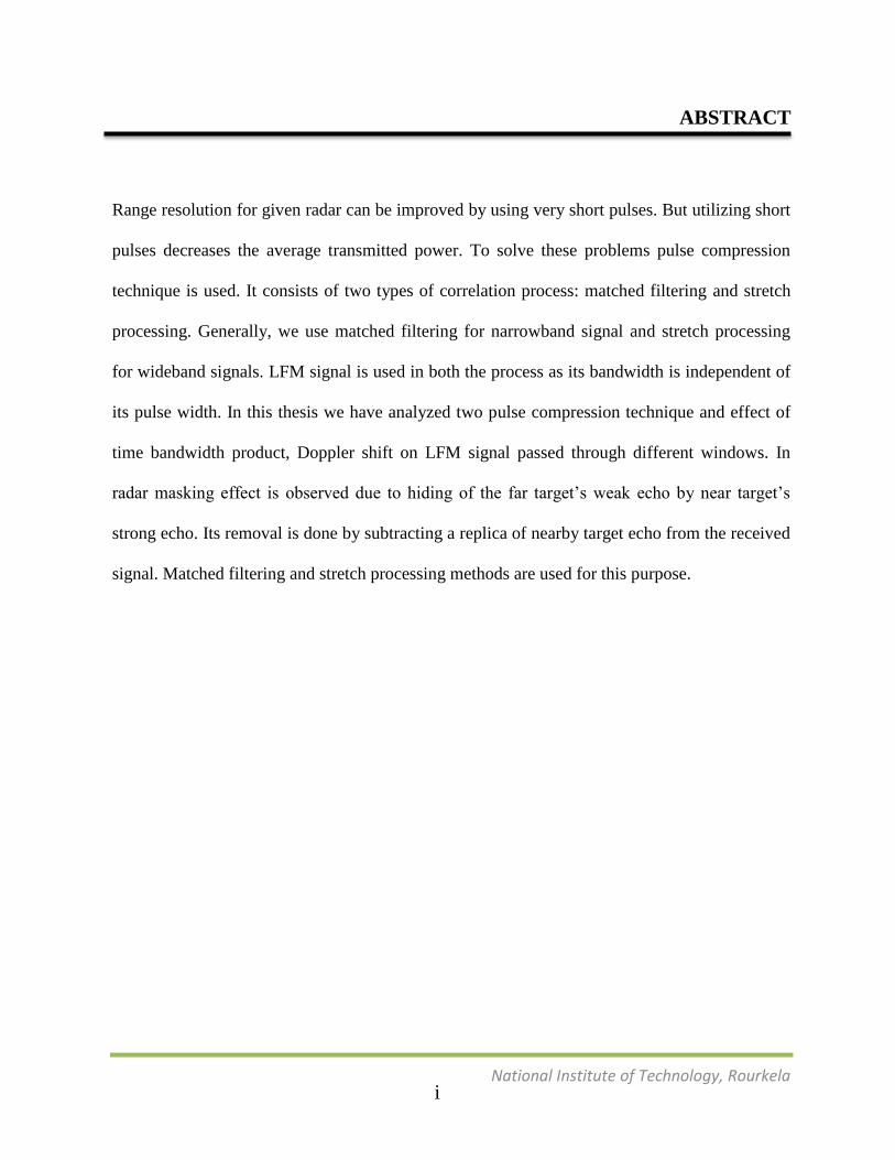
Range resolution for given radar can be improved by using very short pulses. But utilizing short
pulses decreases the average transmitted power. To solve these problems pulse compression
technique is used. It consists of two types of correlation process: matched filtering and stretch
processing. Generally, we use matched filtering for narrowband signal and stretch processing
for wideband signals. LFM signal is used in both the process as its bandwidth is independent of
its pulse width. In this thesis we have analyzed two pulse compression technique and effect of
time bandwidth product, Doppler shift on LFM signal passed through different windows. In
radar masking effect is observed due to hiding of the far target’s weak echo by near target’s
strong echo. Its removal is done by subtracting a replica of nearby target echo from the received
signal. Matched filtering and stretch processing methods are used for this purpose.
i
National Institute of Technology, Rourkela
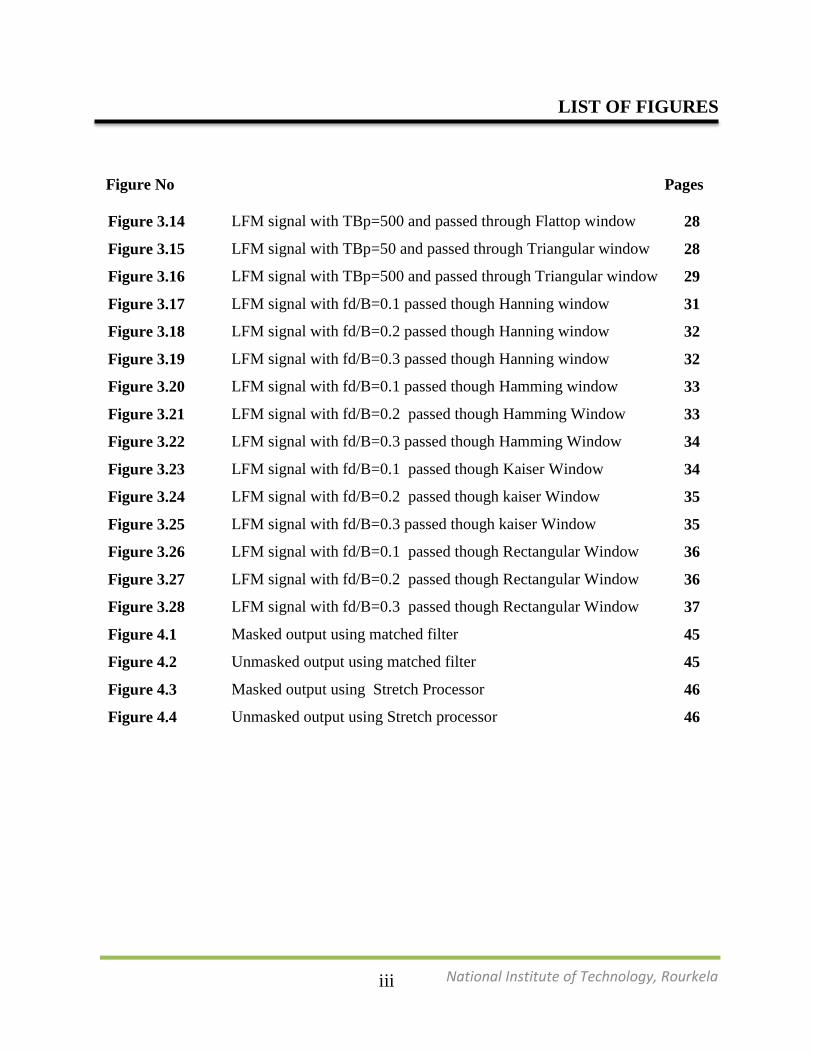
LIST OF FIGURES
Figure No Pages
Figure 1.1 The matched filter receiver 1
Figure 1.2 Geometry for synthetic aperture radar (SAR). 2
Figure 1.3 Block diagram of a SAR system 3
Figure 1.4 SAR image is formed by applying range compression and azimuth
compression algorithms independently.
5
Figure 2.1 Input noise power 8
Figure 2.2 Computation of matched filter output using an FFT 11
Figure 2.3 Match filter output using Kaiser Window. 12
Figure 2.4 Match filter output using Chebyshev window 12
Figure 2.5 Match filtering using hamming window 13
Figure 2.6 Stretch processing output 15
Figure 3.1 LFM signal with TBp=50 and passed through Hanning window 21
Figure 3.2 LFM signal with TBp=500 and passed through Hanning window 22
Figure 3.3 LFM signal with TBp=50 and passed through Hamming window 22
Figure 3.4 LFM signal with TBp=500 and passed through Hamming window 23
Figure 3.5 LFM signal with TBp=50 and passed through kaiser window 23
Figure 3.6 LFM signal with TBp=500 and passed through kaiser window 24
Figure 3.7 LFM signal with TBp=50 and passed through Chebyshev window 24
Figure 3.8 LFM signal with TBp=500 and passed through Chebyshev window 25
Figure 3.9 LFM signal with TBp=50 and passed through Blackmanharris
window
25
Figure 3.10 LFM signal with TBp=500and passed through Blackmanharris
window
26
Figure 3.11 LFM signal with TBp=50 and passed through Nuttal window 26
Figure 3.12 LFM signal with TBp=500 and passed through Nuttal window 27
Figure 3.13 LFM signal with TBp=50 and passed through Flattop window 27
ii
National Institute of Technology, Rourkela
LIST OF FIGURES
Figure No Pages
Figure 3.14 LFM signal with TBp=500 and passed through Flattop window 28
Figure 3.15 LFM signal with TBp=50 and passed through Triangular window 28
Figure 3.16 LFM signal with TBp=500 and passed through Triangular window 29
Figure 3.17 LFM signal with fd/B=0.1 passed though Hanning window 31
Figure 3.18 LFM signal with fd/B=0.2 passed though Hanning window 32
Figure 3.19 LFM signal with fd/B=0.3 passed though Hanning window 32
Figure 3.20 LFM signal with fd/B=0.1 passed though Hamming window 33
Figure 3.21 LFM signal with fd/B=0.2 passed though Hamming Window 33
Figure 3.22 LFM signal with fd/B=0.3 passed though Hamming Window 34
Figure 3.23 LFM signal with fd/B=0.1 passed though Kaiser Window 34
Figure 3.24 LFM signal with fd/B=0.2 passed though kaiser Window 35
Figure 3.25 LFM signal with fd/B=0.3 passed though kaiser Window 35
Figure 3.26 LFM signal with fd/B=0.1 passed though Rectangular Window 36
Figure 3.27 LFM signal with fd/B=0.2 passed though Rectangular Window 36
Figure 3.28 LFM signal with fd/B=0.3 passed though Rectangular Window 37
Figure 4.1 Masked output using matched filter 45
Figure 4.2 Unmasked output using matched filter 45
Figure 4.3 Masked output using Stretch Processor 46
Figure 4.4 Unmasked output using Stretch processor 46
iii
National Institute of Technology, Rourkela
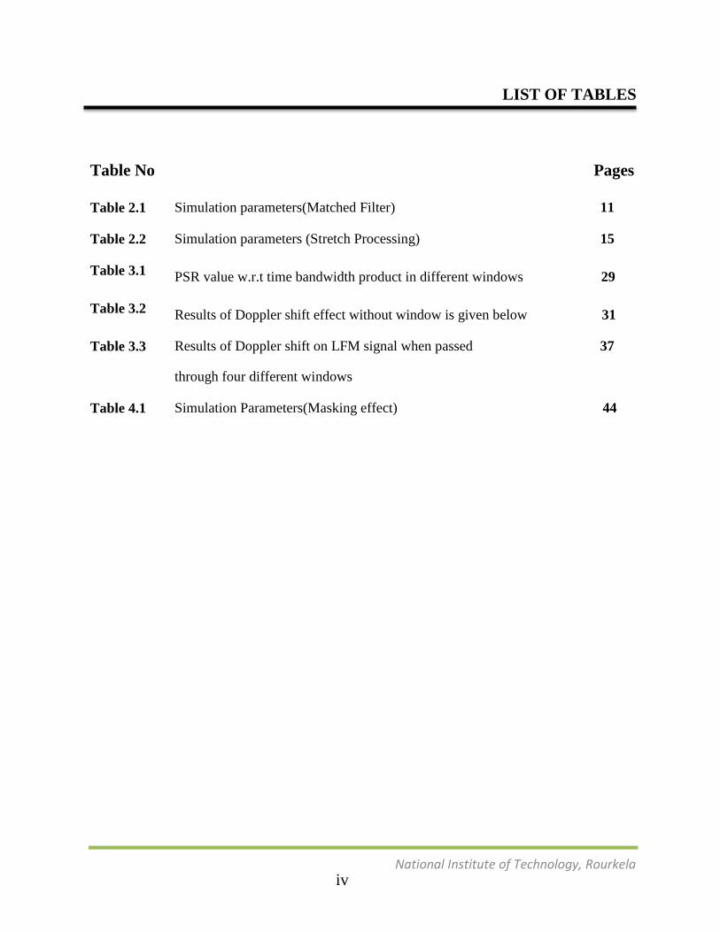
LIST OF TABLES
Table No Pages
Table 2.1 Simulation parameters(Matched Filter) 11
Table 2.2 Simulation parameters (Stretch Processing) 15
Table 3.1 PSR value w.r.t time bandwidth product in different windows 29
Table 3.2 Results of Doppler shift effect without window is given below 31
Table 3.3 Results of Doppler shift on LFM signal when passed 37
through four different windows
Table 4.1 Simulation Parameters(Masking effect) 44
iv
National Institute of Technology, Rourkela
CHAPTER 1 INTRODUCTION
1.1. Pulse compression:
Range compression is achieved by using Linear Frequency Modulated waveform and applying
pulse compression, to achieve a good range resolution. Here, the average transmitted power of a
relatively long pulse is generated, while obtaining the range resolution corresponding to a short
pulse.
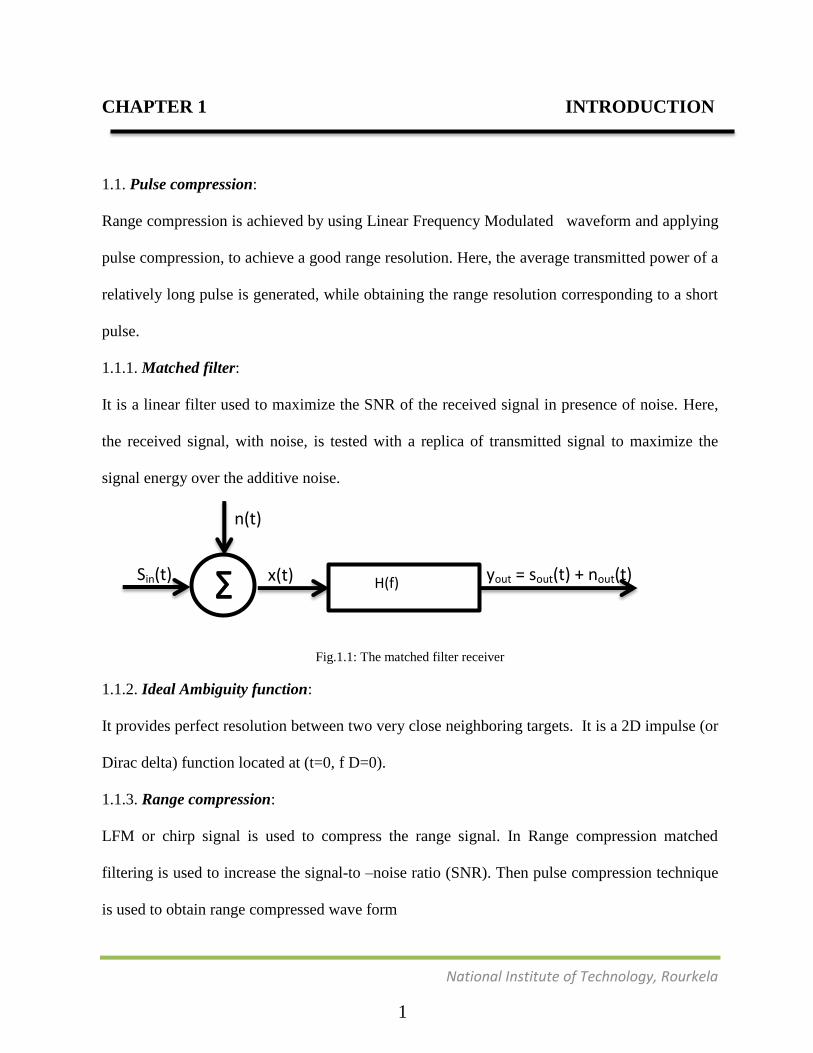
1.1.1. Matched filter:
It is a linear filter used to maximize the SNR of the received signal in presence of noise. Here,
the received signal, with noise, is tested with a replica of transmitted signal to maximize the
signal energy over the additive noise.
Fig.1.1: The matched filter receiver
1.1.2. Ideal Ambiguity function:
It provides perfect resolution between two very close neighboring targets. It is a 2D impulse (or
Dirac delta) function located at (t=0, f D=0).
1.1.3. Range compression:
LFM or chirp signal is used to compress the range signal. In Range compression matched
filtering is used to increase the signal-to –noise ratio (SNR). Then pulse compression technique
is used to obtain range compressed wave form
∑ Sin(t)
n(t)
x(t) yout = sout(t) + nout(t) H(f)
1
National Institute of Technology, Rourkela
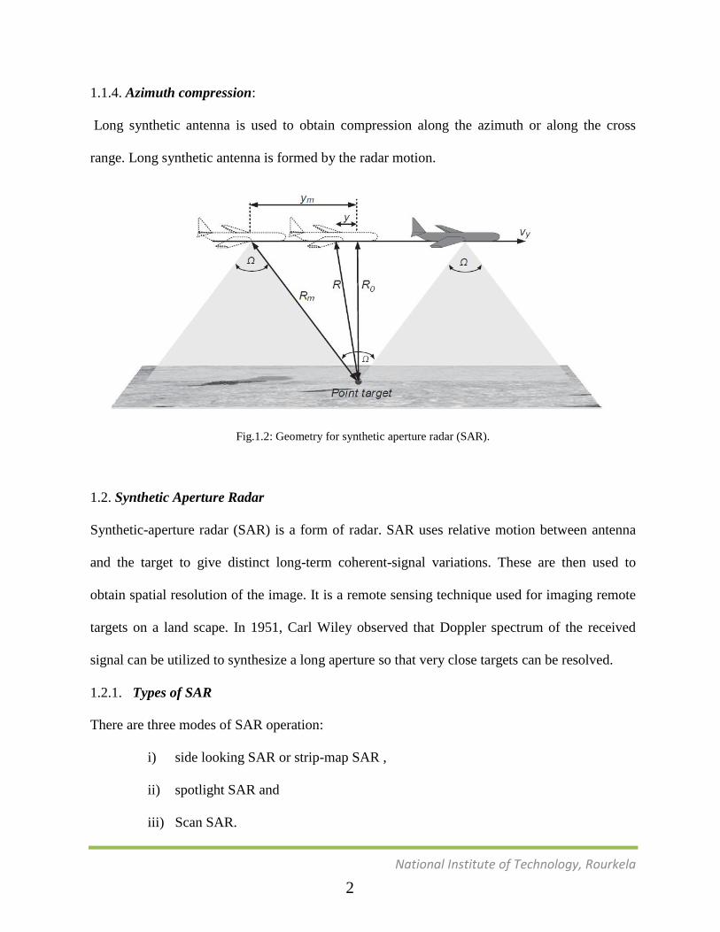
1.1.4. Azimuth compression:
Long synthetic antenna is used to obtain compression along the azimuth or along the cross
range. Long synthetic antenna is formed by the radar motion.
Fig.1.2: Geometry for synthetic aperture radar (SAR).
1.2. Synthetic Aperture Radar
Synthetic-aperture radar (SAR) is a form of radar. SAR uses relative motion between antenna
and the target to give distinct long-term coherent-signal variations. These are then used to
obtain spatial resolution of the image. It is a remote sensing technique used for imaging remote
targets on a land scape. In 1951, Carl Wiley observed that Doppler spectrum of the received
signal can be utilized to synthesize a long aperture so that very close targets can be resolved.
1.2.1. Types of SAR
There are three modes of SAR operation:
i) side looking SAR or strip-map SAR ,
ii) spotlight SAR and
iii) Scan SAR.
2
National Institute of Technology, Rourkela
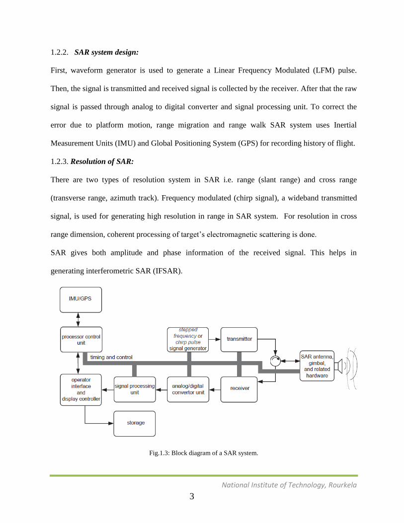
1.2.2. SAR system design:
First, waveform generator is used to generate a Linear Frequency Modulated (LFM) pulse.
Then, the signal is transmitted and received signal is collected by the receiver. After that the raw
signal is passed through analog to digital converter and signal processing unit. To correct the
error due to platform motion, range migration and range walk SAR system uses Inertial
Measurement Units (IMU) and Global Positioning System (GPS) for recording history of flight.
1.2.3. Resolution of SAR:
There are two types of resolution system in SAR i.e. range (slant range) and cross range
(transverse range, azimuth track). Frequency modulated (chirp signal), a wideband transmitted
signal, is used for generating high resolution in range in SAR system. For resolution in cross
range dimension, coherent processing of target’s electromagnetic scattering is done.
SAR gives both amplitude and phase information of the received signal. This helps in
generating interferometric SAR (IFSAR).
Fig.1.3: Block diagram of a SAR system.
3
National Institute of Technology, Rourkela
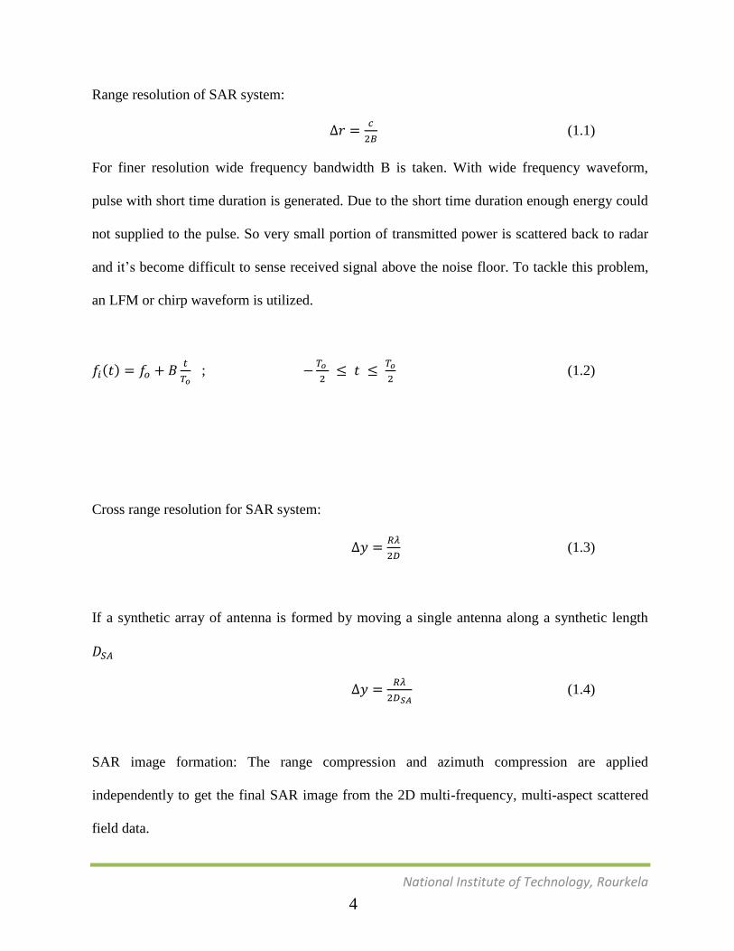
Range resolution of SAR system:
(1.1)
For finer resolution wide frequency bandwidth B is taken. With wide frequency waveform,
pulse with short time duration is generated. Due to the short time duration enough energy could
not supplied to the pulse. So very small portion of transmitted power is scattered back to radar
and it’s become difficult to sense received signal above the noise floor. To tackle this problem,
an LFM or chirp waveform is utilized.
( )
;
(1.2)
Cross range resolution for SAR system:
(1.3)
If a synthetic array of antenna is formed by moving a single antenna along a synthetic length
(1.4)
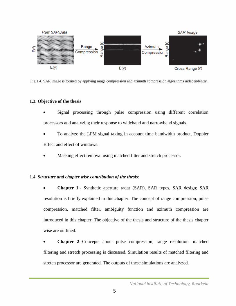
SAR image formation: The range compression and azimuth compression are applied
independently to get the final SAR image from the 2D multi-frequency, multi-aspect scattered
field data.
4
National Institute of Technology, Rourkela
Fig.1.4. SAR image is formed by applying range compression and azimuth compression algorithms independently.
1.3. Objective of the thesis
Signal processing through pulse compression using different correlation
processors and analyzing their response to wideband and narrowband signals.
To analyze the LFM signal taking in account time bandwidth product, Doppler
Effect and effect of windows.
Masking effect removal using matched filter and stretch processor.
1.4. Structure and chapter wise contribution of the thesis:
Chapter 1:- Synthetic aperture radar (SAR), SAR types, SAR design; SAR
resolution is briefly explained in this chapter. The concept of range compression, pulse
compression, matched filter, ambiguity function and azimuth compression are
introduced in this chapter. The objective of the thesis and structure of the thesis chapter
wise are outlined.
Chapter 2:-Concepts about pulse compression, range resolution, matched
filtering and stretch processing is discussed. Simulation results of matched filtering and
stretch processor are generated. The outputs of these simulations are analyzed.
5
National Institute of Technology, Rourkela
Chapter 3:- Concept of LFM signal is outlined. Effect of windows, Doppler
shift and time band width product is discussed. Simulations are results are analyzed and
conclusion is out lined.
Chapter 4:- Masking effect on radar signal is discussed. Removal of masking
effect using matched filtering and stretch processor is explained and the simulation
results are discussed.
1.4. Conclusion
Synthetic aperture radar (SAR), SAR types, SAR design, SAR resolution is briefly explained in
this chapter. The concept of range compression, pulse compression, matched filter, ambiguity
function and azimuth compression are introduced in this chapter. The objective of the thesis and
structure of the thesis chapter wise are outlined. Objective of the thesis and structure of the
thesis is outlined.
6
National Institute of Technology, Rourkela
CHAPTER 2 PULSE COMPRESSION
2.1 Introduction
There are two types of resolution system in SAR i.e. range (slant range) and cross range
(transverse range, azimuth track). Frequency modulated (chirp signal), a wideband transmitted
signal, is used for generating high resolution in range in SAR system. For resolution in cross
range dimension, coherent processing of target’s electromagnetic scattering is done.
Very short pulses are required for generating good resolution in a SAR. But the average power
transmitting through the signal decreases with the use of short pulses, This in turn, affect the
SAR’s normal modes of operation drastically, mostly when we use multi-function and
surveillance SARs. The average transmitted power is directly proportional to the receiver signal
to noise ratio. It is often desirable to increase the pulse width is therefore increased (i.e.,
increase the average transmitted power) while, maintaining adequate range resolution at the
same time. Pulse compression techniques are considered for implementing this process. Pulse
compression generally helps us to generate the average transmitted power of a comparatively
long pulse, while generating the range resolution with respect to a short pulse. Normally, there
are two types of pulse compression technique: analyze analog and digital pulse compression
techniques. Two analog pulse compression techniques are described in this chapter. One is
correlation processing. This technique is mainly used for narrow band and some medium band
radar operations. The other one is “stretch processing”. This is normally used for very wide
band radar operations. Digital pulse compression is also discussed briefly in this chapter.
7
National Institute of Technology, Rourkela
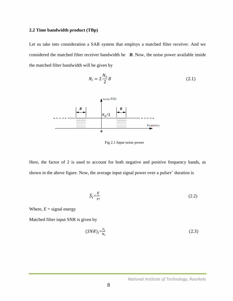
2.2 Time bandwidth product (TBp)
Let us take into consideration a SAR system that employs a matched filter receiver. And we
considered the matched filter receiver bandwidth be B. Now, the noise power available inside
the matched filter bandwidth will be given by
( )
Fig 2.1 Input noise power
Here, the factor of 2 is used to account for both negative and positive frequency bands, as
shown in the above figure. Now, the average input signal power over a pulse ’ duration is
=
(2.2)
Where, E = signal energy
Matched filter input SNR is given by
( ) =
( )
8
National Institute of Technology, Rourkela
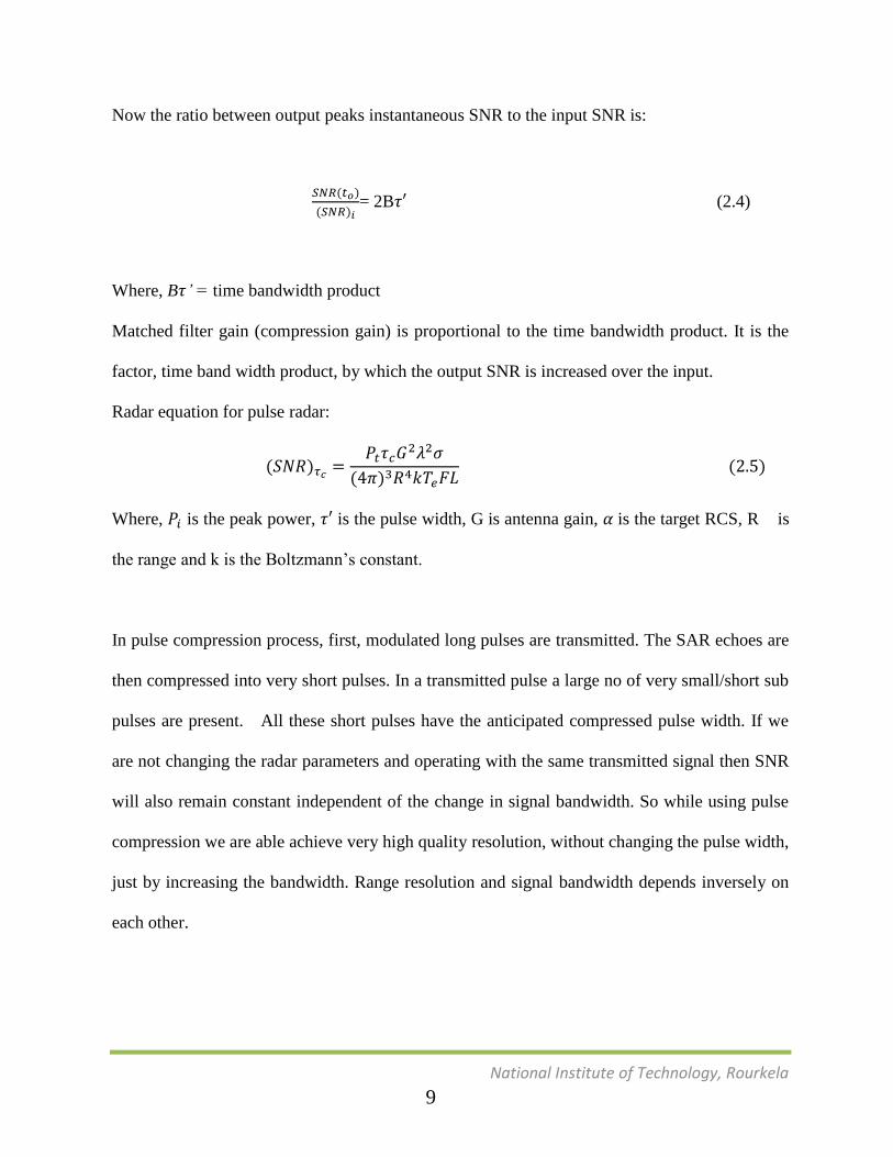
Now the ratio between output peaks instantaneous SNR to the input SNR is:
( )
( ) = 2B (2.4)
Where, B ’ = time bandwidth product
Matched filter gain (compression gain) is proportional to the time bandwidth product. It is the
factor, time band width product, by which the output SNR is increased over the input.
Radar equation for pulse radar:
( )
( ) ( )
Where, is the peak power, is the pulse width, G is antenna gain, is the target RCS, R is
the range and k is the Boltzmann’s constant.
In pulse compression process, first, modulated long pulses are transmitted. The SAR echoes are
then compressed into very short pulses. In a transmitted pulse a large no of very small/short sub
pulses are present. All these short pulses have the anticipated compressed pulse width. If we
are not changing the radar parameters and operating with the same transmitted signal then SNR
will also remain constant independent of the change in signal bandwidth. So while using pulse
compression we are able achieve very high quality resolution, without changing the pulse width,
just by increasing the bandwidth. Range resolution and signal bandwidth depends inversely on
each other.
9
National Institute of Technology, Rourkela
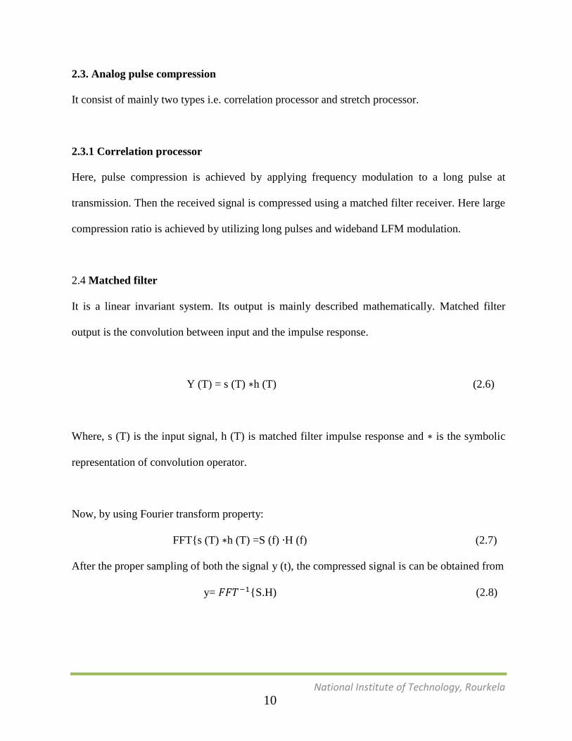
2.3. Analog pulse compression
It consist of mainly two types i.e. correlation processor and stretch processor.
2.3.1 Correlation processor
Here, pulse compression is achieved by applying frequency modulation to a long pulse at
transmission. Then the received signal is compressed using a matched filter receiver. Here large
compression ratio is achieved by utilizing long pulses and wideband LFM modulation.
2.4 Matched filter
It is a linear invariant system. Its output is mainly described mathematically. Matched filter
output is the convolution between input and the impulse response.
Y (T) = s (T) h (T) (2.6)
Where, s (T) is the input signal, h (T) is matched filter impulse response and is the symbolic
representation of convolution operator.
Now, by using Fourier transform property:
FFT{s (T) h (T) =S (f) H (f) (2.7)
After the proper sampling of both the signal y (t), the compressed signal is can be obtained from
y= {S.H) (2.8)
10
National Institute of Technology, Rourkela
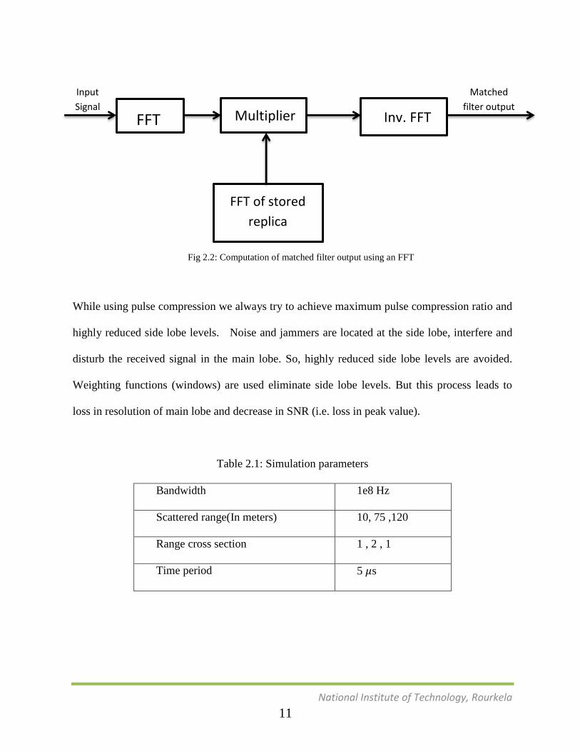
Fig 2.2: Computation of matched filter output using an FFT
While using pulse compression we always try to achieve maximum pulse compression ratio and
highly reduced side lobe levels. Noise and jammers are located at the side lobe, interfere and
disturb the received signal in the main lobe. So, highly reduced side lobe levels are avoided.
Weighting functions (windows) are used eliminate side lobe levels. But this process leads to
loss in resolution of main lobe and decrease in SNR (i.e. loss in peak value).
Table 2.1: Simulation parameters
Bandwidth 1e8 Hz
Scattered range(In meters) 10, 75 ,120
Range cross section 1 , 2 , 1
Time period 5 s
Matched
filter output Inv. FFT Multiplier
Input
Signal
FFT
FFT of stored
replica
11
National Institute of Technology, Rourkela
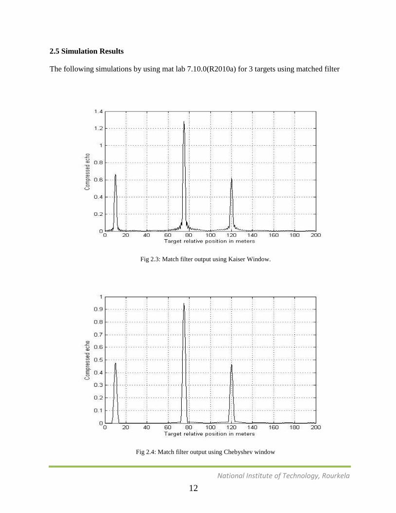
2.5 Simulation Results
The following simulations by using mat lab 7.10.0(R2010a) for 3 targets using matched filter
Fig 2.3: Match filter output using Kaiser Window.
Fig 2.4: Match filter output using Chebyshev window
12
National Institute of Technology, Rourkela
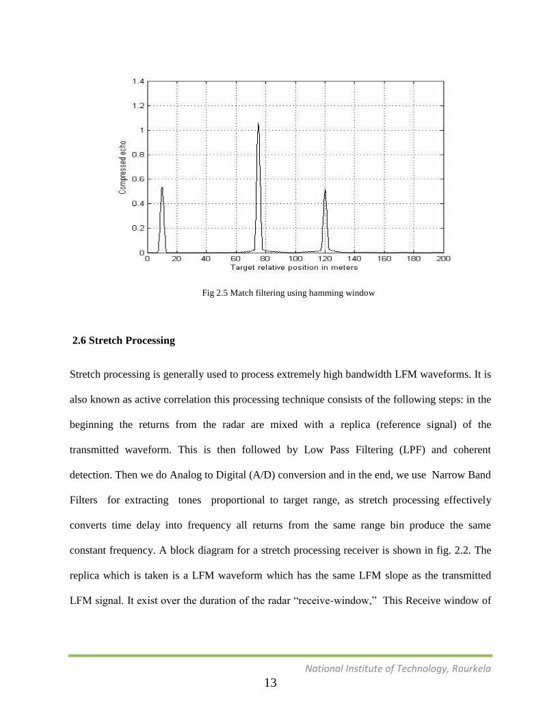
Fig 2.5 Match filtering using hamming window
2.6 Stretch Processing
Stretch processing is generally used to process extremely high bandwidth LFM waveforms. It is
also known as active correlation this processing technique consists of the following steps: in the
beginning the returns from the radar are mixed with a replica (reference signal) of the
transmitted waveform. This is then followed by Low Pass Filtering (LPF) and coherent
detection. Then we do Analog to Digital (A/D) conversion and in the end, we use Narrow Band
Filters for extracting tones proportional to target range, as stretch processing effectively
converts time delay into frequency all returns from the same range bin produce the same
constant frequency. A block diagram for a stretch processing receiver is shown in fig. 2.2. The
replica which is taken is a LFM waveform which has the same LFM slope as the transmitted
LFM signal. It exist over the duration of the radar “receive-window,” This Receive window of
13
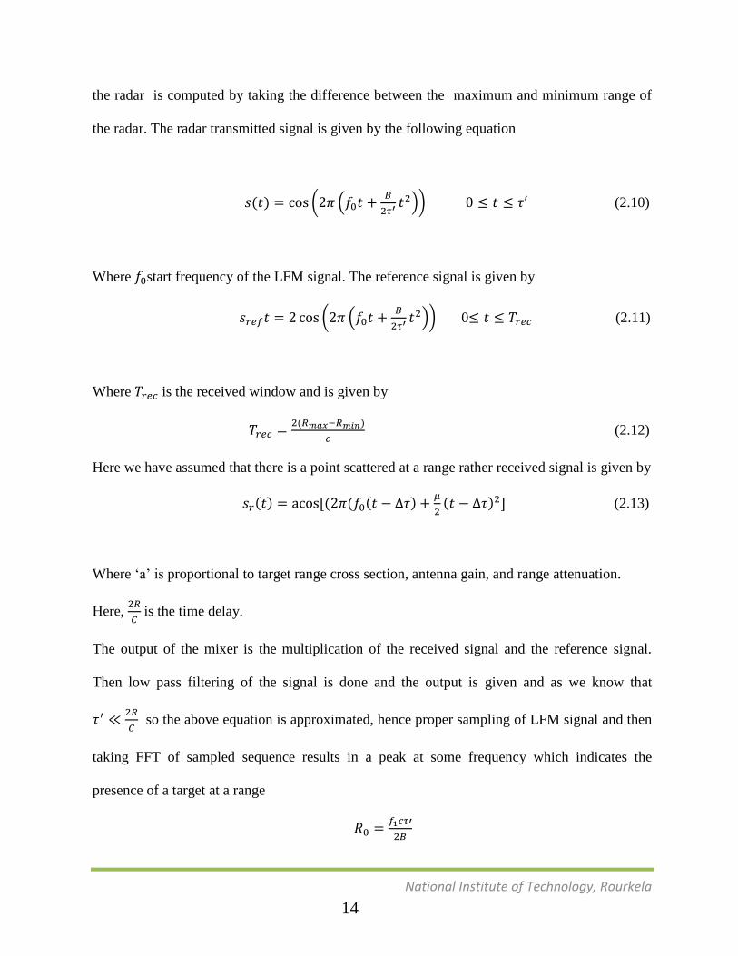
National Institute of Technology, Rourkela
the radar is computed by taking the difference between the maximum and minimum range of
the radar. The radar transmitted signal is given by the following equation
( ) ( (
)) (2.10)
Where start frequency of the LFM signal. The reference signal is given by
( (
)) 0 (2.11)
Where is the received window and is given by
( )
(2.12)
Here we have assumed that there is a point scattered at a range rather received signal is given by
( ) ( ( ( )
( ) (2.13)
Where ‘a’ is proportional to target range cross section, antenna gain, and range attenuation.
Here,
is the time delay.
The output of the mixer is the multiplication of the received signal and the reference signal.
Then low pass filtering of the signal is done and the output is given and as we know that
so the above equation is approximated, hence proper sampling of LFM signal and then
taking FFT of sampled sequence results in a peak at some frequency which indicates the
presence of a target at a range
14
National Institute of Technology, Rourkela
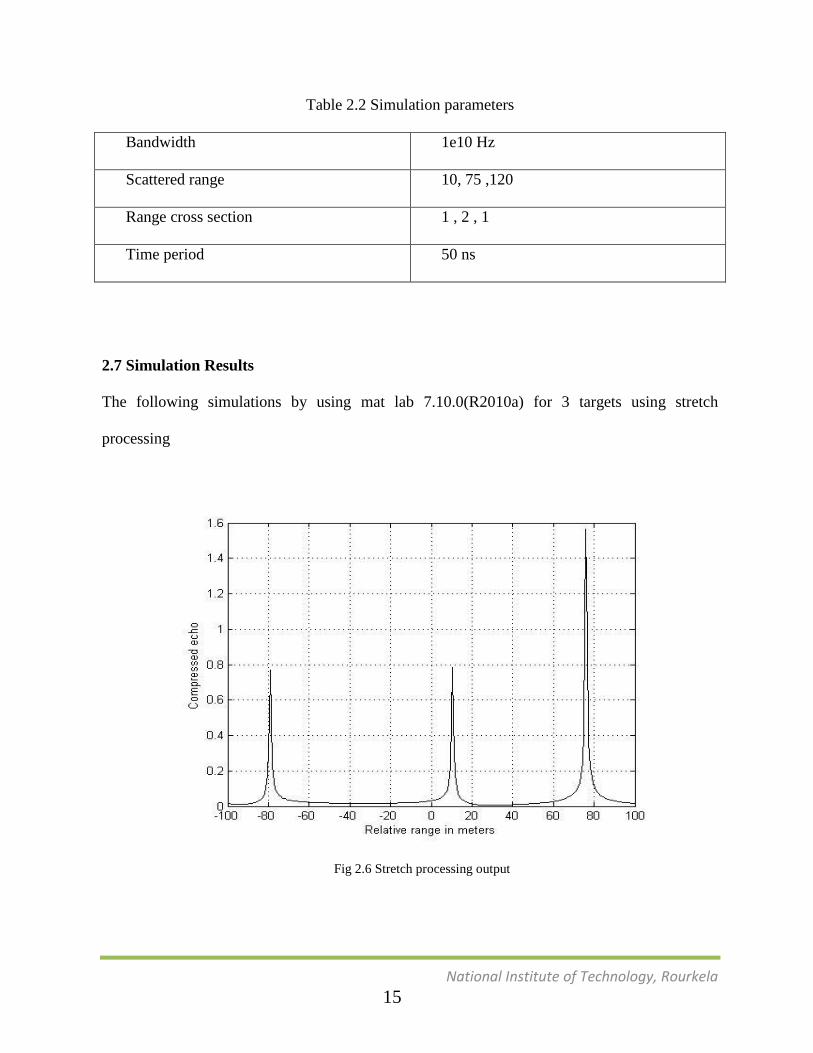
Table 2.2 Simulation parameters
Bandwidth 1e10 Hz
Scattered range 10, 75 ,120
Range cross section 1 , 2 , 1
Time period 50 ns
2.7 Simulation Results
The following simulations by using mat lab 7.10.0(R2010a) for 3 targets using stretch
processing
Fig 2.6 Stretch processing output
15
National Institute of Technology, Rourkela
2.8 Conclusion
In Pulse compression of radar signal to get the resolved range coming from three targets, two of
its techniques were analyzed, Matched Filtering and Stretched Processing. It is found that
matched filter improves the SNR (signal to noise ratio) and attenuates the side lobes. While in
Stretch processing complete elimination of side lobes can be seen. Matched filter is mainly
suitable for narrow band signal and shows complexity while used for wideband signals. On the
other hand stretch processing is suitable for wideband signals. Wideband signals are easily
processed by stretched processing technique than matched filtering technique, which takes a lot
of time for processing wideband signals and even not compatible for wideband signals beyond
a certain limit.
16
National Institute of Technology, Rourkela
CHAPTER 3 LINEAR FREQUENCY MODULATION (LFM)
3.1 Introduction:
Pulsed Radar has a range resolution of
(3.1)
Where, B=bandwidth of the pulse.
C=velocity of light in vacuum.
The Fourier theory says, the frequency bandwidth, Bob the signal is inversely proportional to
pulse duration in the following manner as
B
(3.2)
This shows that the range resolution is directly promotional to its pulse duration in the
following manner
(3.3)
Hence for a good range resolution we need to keep the duration of a pulse small. But the
problem with short pulses is that it will not be possible to put enough energy on this pulse.
Sufficiently wide pulse cannot achieve a wide bandwidth because if we are using an un-
modulated pulse having constant frequency, its time duration will be very small and will not be
possible to enough energy on it. This problem can be solved by using a modulated pulse of
sufficient duration so that it will provide the required bandwidth for the operation of radar. The
most common waveform used for this purpose is the LFM (Linear frequency modulated) pulse,
17
National Institute of Technology, Rourkela
also known as the chirp pulse. .This waveform repeats itself in every interval called PRI (pulse
repetition interval) or also known as pulse repetition period .The LFM signal taken over here is
given by:
( ) (
)
(3.4)
Where, B=bandwidth of the signal and T=time period
3.2 Effect of windows on side lobe reduction of LFM signal
Window functions are mathematical expressions which are having a particular value in an
interval and have no value outside it. One example of a window is a rectangular window that is
constant inside the interval and zero elsewhere .It describes the shape of its graphical
representation. When the window is multiplied by another function or waveform, their product
is also zero-valued outside the interval. And all that the part where they overlap, only exists.
The LFM signal was introduced to following 8 windows:
3.2.1 Rectangular window
The rectangular window has one value over its length. It has the following equation.
w(n) = 1.0 for n = 0, 1, 2, …, N – 1 (3.5)
Where N is the length of the window and w is the window value.
A rectangular window when applied just limits the signal to within a finite time interval.
Therefore it is equivalent to not using any window.
18

National Institute of Technology, Rourkela
3.2.2 Hanning window
The Henning window resembles half a cycle of a cosine wave. The Henning window has the
following equation
(
(3.6)
For n = 0, 1, 2, N – 1
Where N is the length of the window and w is the window value. `
3.2.3. Hamming window
It is a modified version of the Henning window. It has a shape like a cosine wave. Hamming
window is described by the following window.
( )
(3.7)
For n = 0, 1, 2, N – 1
Where N is the length of the window and w is the window value.
3.2.4 Kaiser window
The Kaiser window is a flexible smoothing window whose shape can be modified by adjusting
the beta (β) parameter. w = Kaiser (L, beta) returns an L-point Kaiser window in the column
vector w. beta is the Kaiser Window β parameter that affects the side lobe attenuation of the
Fourier transform of the window.
19

National Institute of Technology, Rourkela
3.2.5. Blackmannharris window
It does the window sampling by using 'sflag'. This can either be 'periodic' or 'symmetric' (the default).
The 'periodic' flag is generally used for Fourier transform, so that spectral analysis can be done. Its
equation is given by:
(
) (
) (
) (3.9)
Where
and the window length is given by L=N+1
3.2.6 Flattop window
Flat Top window has very low pass band ripple (< 0.01 dB) they are generally used for
calibration purposes. They have a bandwidth equivalent to approximately 2.5 times wider than a
Han window. Its equation is given by:
( ) (
)+ (
) (
) (
) (3.10)
Where 0 and w (n) =0elsewhere and the window length is L=N+1.
3.2.7 Nuttall window
( ) (
) (
) (
) (3.11)
3.2.8 Triangular window
(3.12)
20
National Institute of Technology, Rourkela
3.2.9 PSR
It is called peak to side lobe ratio (PSR). It is given by
(3.13)
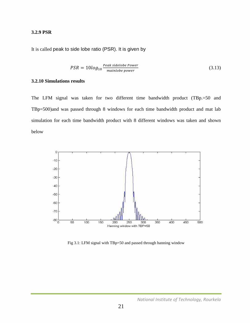
3.2.10 Simulations results
The LFM signal was taken for two different time bandwidth product (TBp.=50 and
TBp=500)and was passed through 8 windows for each time bandwidth product and mat lab
simulation for each time bandwidth product with 8 different windows was taken and shown
below
Fig 3.1: LFM signal with TBp=50 and passed through hanning window
21
National Institute of Technology, Rourkela
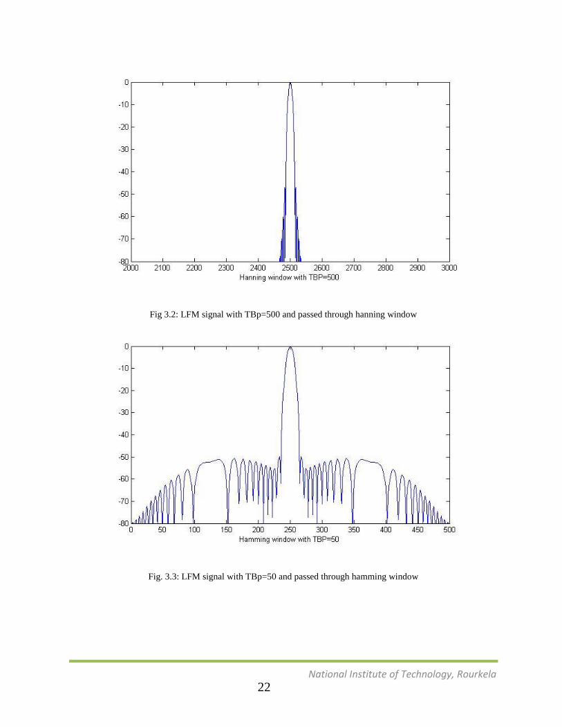
Fig 3.2: LFM signal with TBp=500 and passed through hanning window
Fig. 3.3: LFM signal with TBp=50 and passed through hamming window
22
National Institute of Technology, Rourkela
Fig 3.4 LFM signal with TBp=500 and passed through hamming window
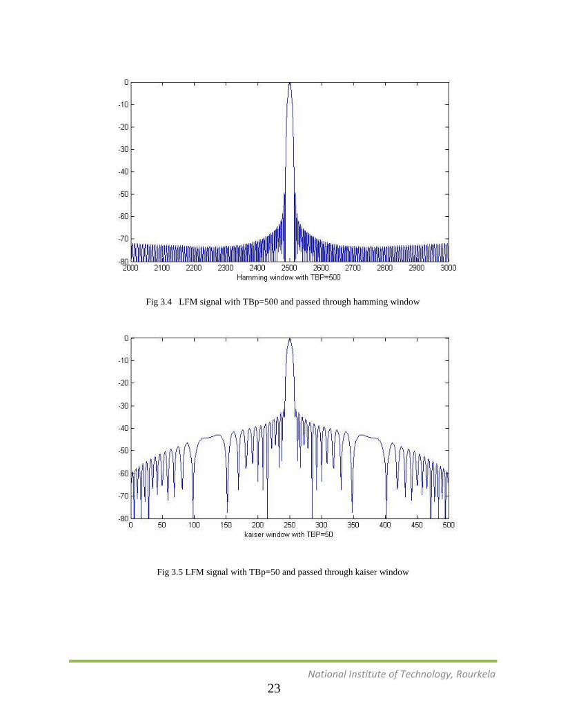
Fig 3.5 LFM signal with TBp=50 and passed through kaiser window
23
National Institute of Technology, Rourkela
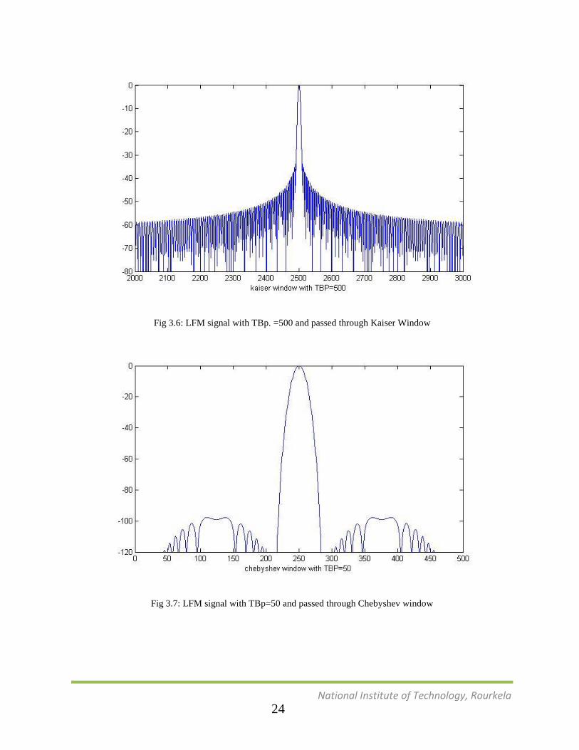
Fig 3.6: LFM signal with TBp. =500 and passed through Kaiser Window
Fig 3.7: LFM signal with TBp=50 and passed through Chebyshev window
24
National Institute of Technology, Rourkela
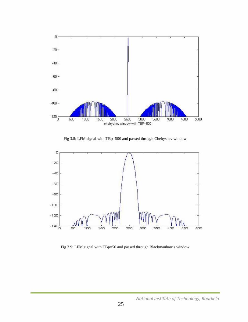
Fig 3.8: LFM signal with TBp=500 and passed through Chebyshev window
Fig 3.9: LFM signal with TBp=50 and passed through Blackmanharris window
25
National Institute of Technology, Rourkela
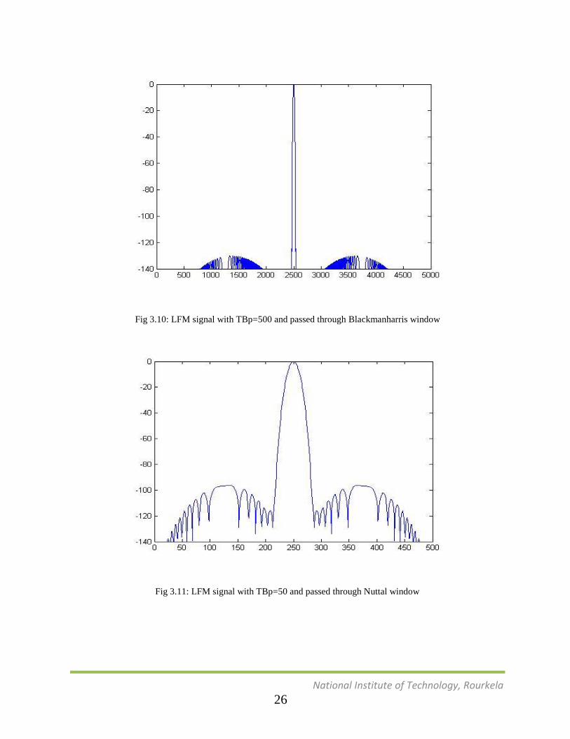
Fig 3.10: LFM signal with TBp=500 and passed through Blackmanharris window
Fig 3.11: LFM signal with TBp=50 and passed through Nuttal window
26
National Institute of Technology, Rourkela
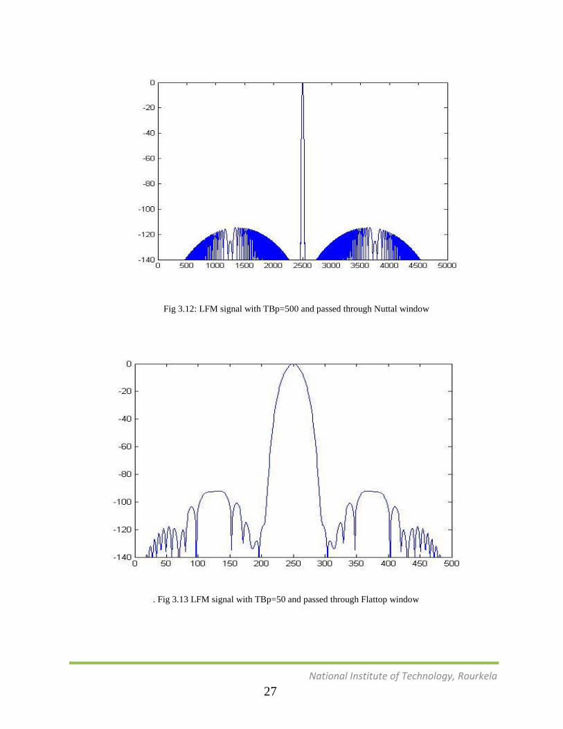
Fig 3.12: LFM signal with TBp=500 and passed through Nuttal window
. Fig 3.13 LFM signal with TBp=50 and passed through Flattop window
27
National Institute of Technology, Rourkela
.
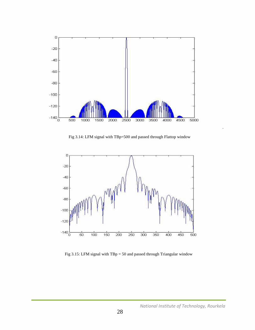
Fig 3.14: LFM signal with TBp=500 and passed through Flattop window
Fig 3.15: LFM signal with TBp = 50 and passed through Triangular window
28
National Institute of Technology, Rourkela
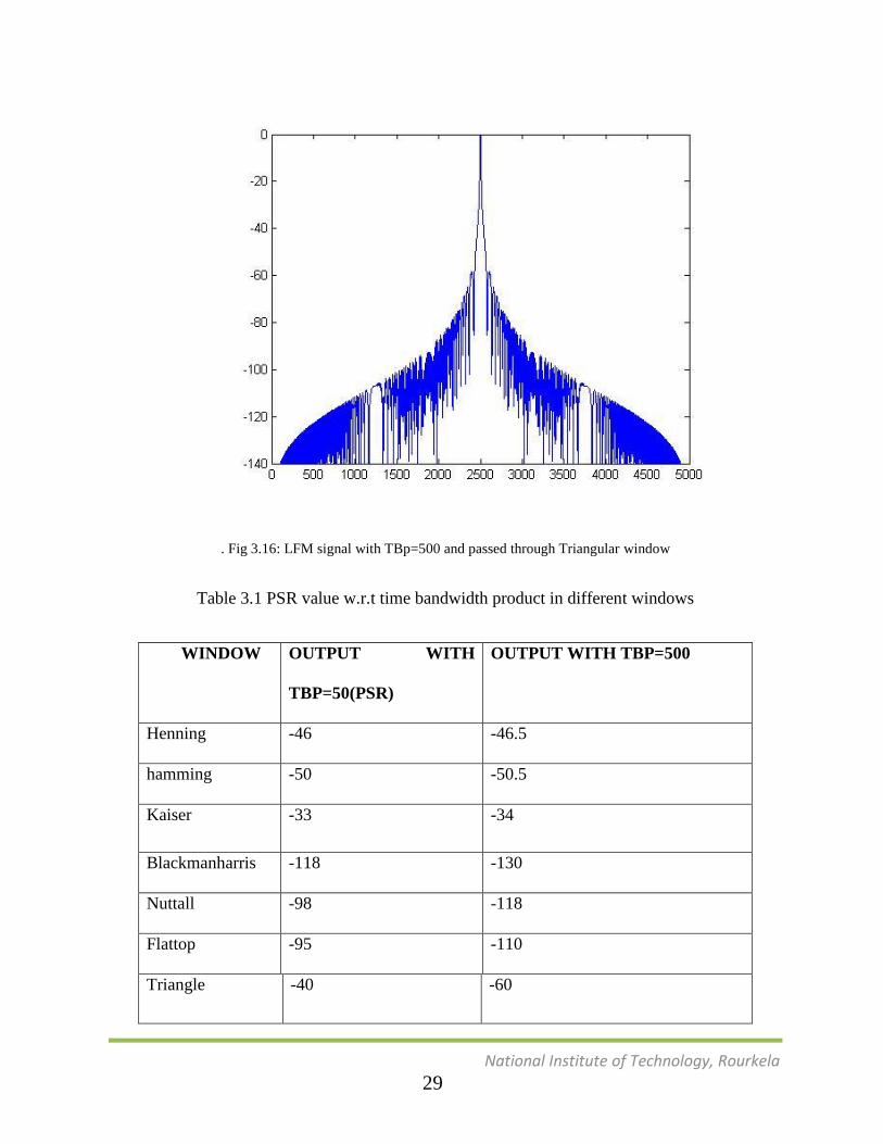
. Fig 3.16: LFM signal with TBp=500 and passed through Triangular window
Table 3.1 PSR value w.r.t time bandwidth product in different windows
WINDOW OUTPUT WITH
TBP=50(PSR)
OUTPUT WITH TBP=500
Henning -46 -46.5
hamming -50 -50.5
Kaiser -33 -34
Blackmanharris -118 -130
Nuttall -98 -118
Flattop -95 -110
Triangle -40 -60
29
National Institute of Technology, Rourkela
3.2.11 Result
From the above we draw the following conclusions:-
1. Blackmanharris window has the best Side lobe reduction where rectangular window has
the worst Side lobe reduction.
2. The Side lobe reduction is least affected by time bandwidth product. In some windows,
they are with a little bit of variation in generalized hamming window. Whereas in higher
order generalized cosine windows like Blackmanharris, Nuttall and flattop window PSR
is large with the change in bandwidth time product.
3. In Kaiser Window the ‘β’ parameter provides a relation between reduction in side-lobe
level and main-lobe width. Larger values of β gives lower side-lobe levels, but at the
same time it widens the main lobe. But widening the main lobe results in reduction in
frequency resolution when the window is used for spectrum analysis.
3.3 Doppler effects on LFM signals
RADAR signals encounter Doppler Effect when there is a moving target. Radars use the
Doppler frequency to extract target radial velocity. Here we will observe the effect of Doppler
frequency on LFM signal. FM signal without adding Doppler frequency is given below.
( ((
)( )))
(3.14)
LFM signal with A Doppler shift is given by
( ((
) ( ) ))
(3.15)
Where, =Doppler frequency
30
National Institute of Technology, Rourkela
Table 3.2 Results of Doppler shift effect without window is given below
-13.8 -13.2 -13.2
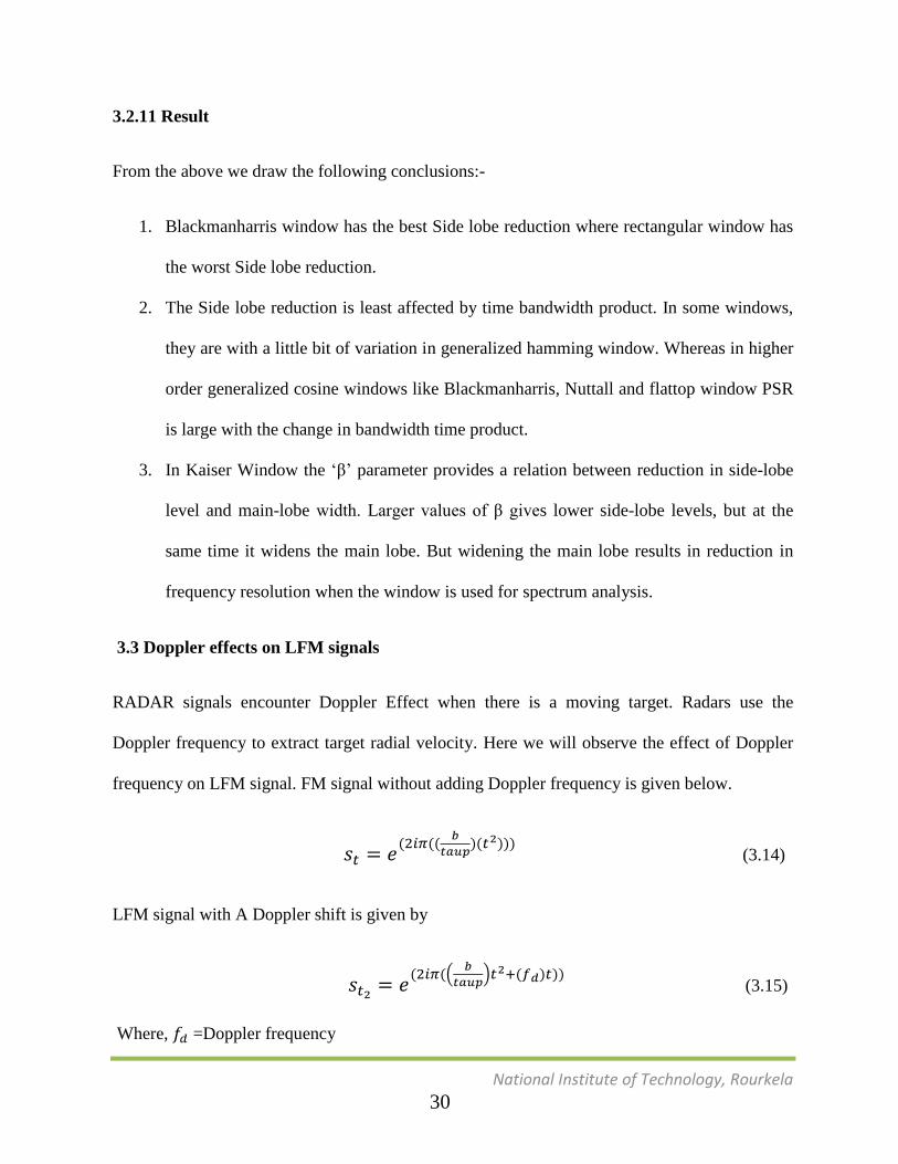
3.3.1 Simulation Results
The LFM signal was added with varying Doppler shift ( ) and its effect on passing the LFM
signal with four windows was studied
Fig3.17. LFM signal with fd/B=0.1 passed though Hanning window
31
National Institute of Technology, Rourkela
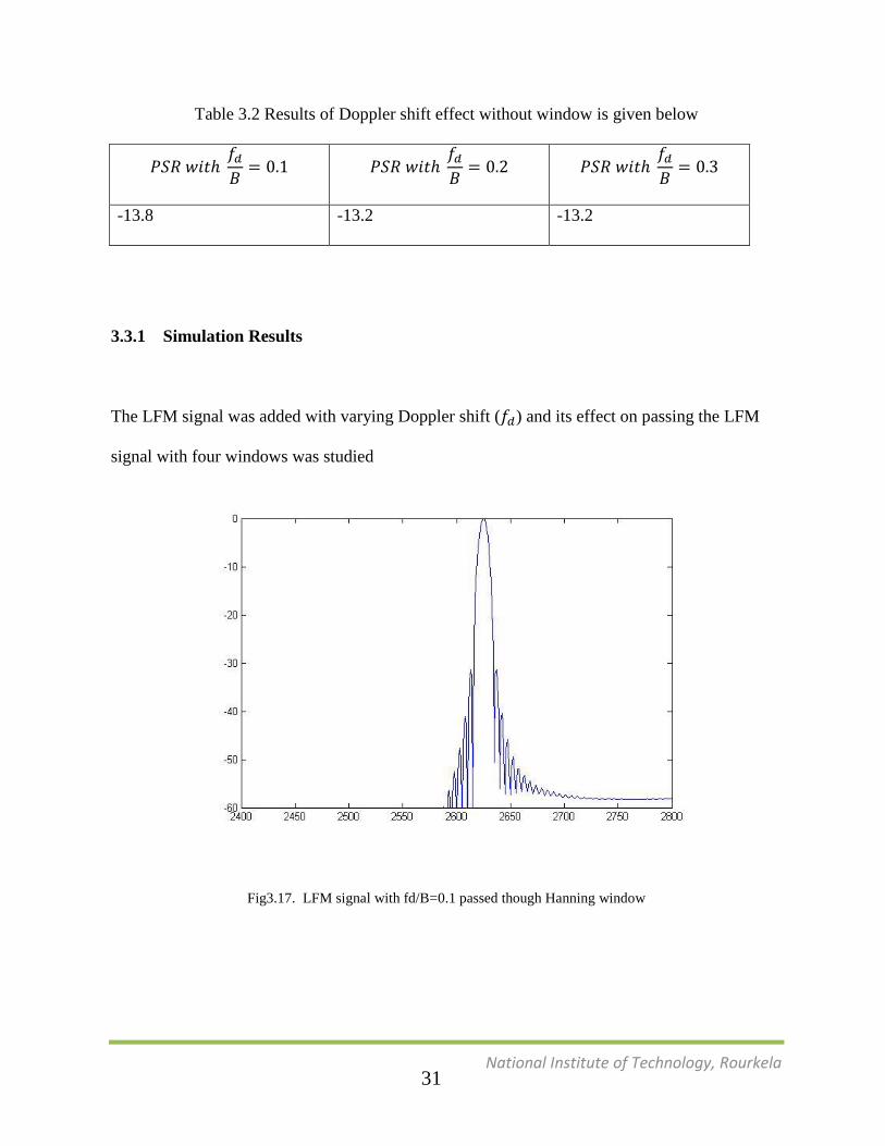
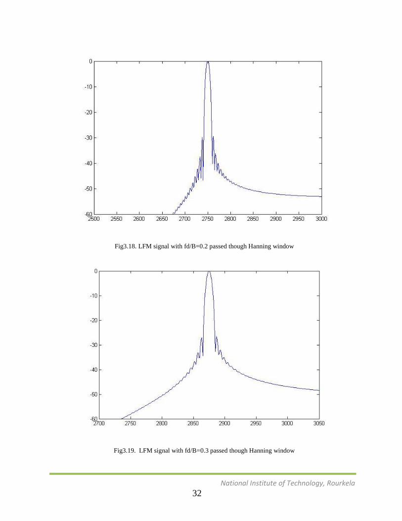
Fig3.18. LFM signal with fd/B=0.2 passed though Hanning window
Fig3.19. LFM signal with fd/B=0.3 passed though Hanning window
32
National Institute of Technology, Rourkela
.
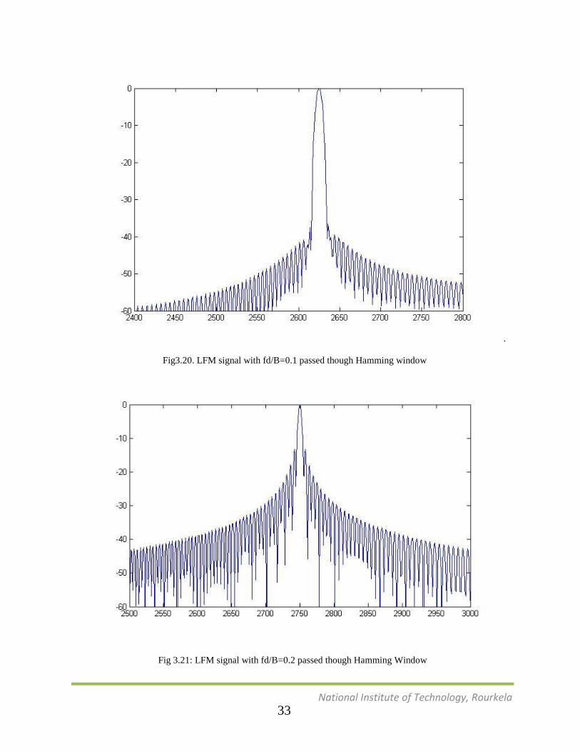
Fig3.20. LFM signal with fd/B=0.1 passed though Hamming window
Fig 3.21: LFM signal with fd/B=0.2 passed though Hamming Window
33
National Institute of Technology, Rourkela
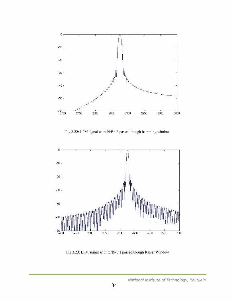
Fig 3.22: LFM signal with fd/B=.3 passed though hamming window
Fig 3.23: LFM signal with fd/B=0.1 passed though Kaiser Window
34
National Institute of Technology, Rourkela
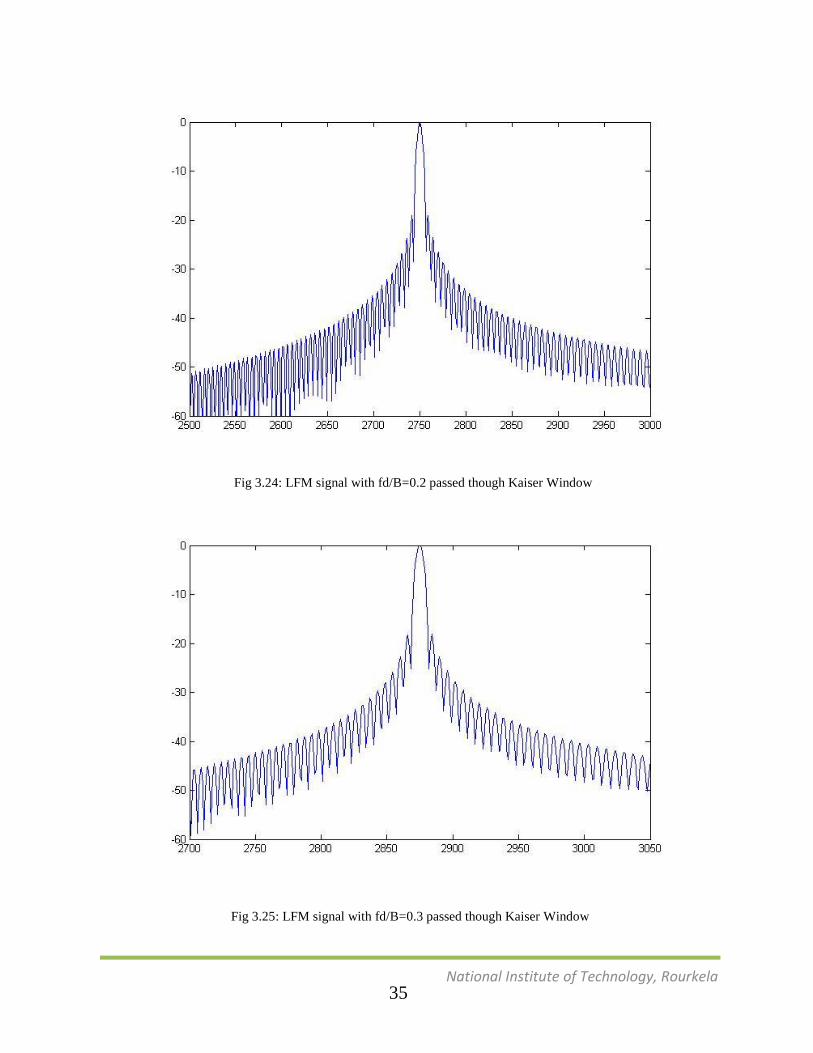
Fig 3.24: LFM signal with fd/B=0.2 passed though Kaiser Window
Fig 3.25: LFM signal with fd/B=0.3 passed though Kaiser Window
35
National Institute of Technology, Rourkela
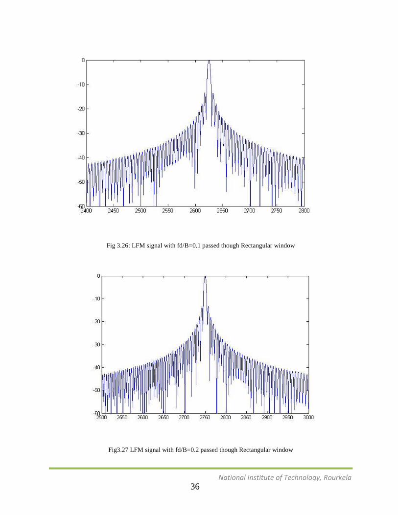
Fig 3.26: LFM signal with fd/B=0.1 passed though Rectangular window
Fig3.27 LFM signal with fd/B=0.2 passed though Rectangular window
36
National Institute of Technology, Rourkela
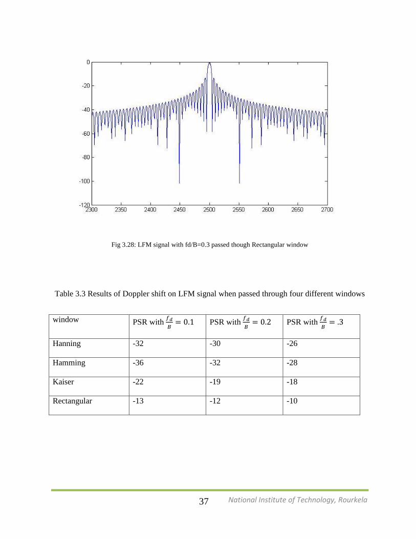
Fig 3.28: LFM signal with fd/B=0.3 passed though Rectangular window
Table 3.3 Results of Doppler shift on LFM signal when passed through four different windows
window PSR with
PSR with
PSR with
Hanning -32 -30 -26
Hamming -36 -32 -28
Kaiser -22 -19 -18
Rectangular -13 -12 -10
37
National Institute of Technology, Rourkela
3.4 Result
1. The Doppler shift effect is not felt so much in the absence of window and the PSR for three
different values of fd/B(where B=bandwidth).The PSR remains almost the same for the three
values.
2. The Doppler shift effect is then checked by passing the signal through 4 windows (Hanning,
Hamming, Kaiser, and Rectangular) and we found out that PSR decreased with increase in
Doppler Effect.
3.5 Conclusion
LFM (Linear Frequency Modulated) signals are the most popularly used signals for radar signal
processing. In this chapter LFM signal was analyzed taking into account time bandwidth
product and Doppler effect For analyzing effect of time bandwidth product on LFM signal, it
was passed with nine windows and time bandwidth product was taken 50 for 1st case and time
bandwidth product was taken 500 for 2nd
case. It is observed that the PSR (Peak to Signal Ratio)
increases with increase in time bandwidth product. Next LFM signal was Doppler shifted and it
is observed that the PSR decreases with increase in Doppler shift. It is also observed that the
LFM signal, when passed through Blackmanharris window, the Side lobe suppression is
maximum.
38

National Institute of Technology, Rourkela
CHAPTER 4 MASKING EFFECT REMOVAL
4.1 Introduction
Signal processing in noise radar is based on the calculation of the correlation between
transmitted and received signals. Received signals collected from nearby targets produce very
high side lobes in the correlation function. While the signals received from far targets are weak
.These weak echoes of far targets are masked by the strong echoes, this effect is called as
masking effect. Masking effect can be removed by methods. Considering only the Doppler
shift of target echoes for removal of masking effect is one of the old methods. But, this method
does not remove the strong target echo completely when targets migrate between range
resolution cells in the integration time. The signal stretch processing based method, gives an
improved result over the existing methods. The detection of weak targets in the presence of the
fast and strong ones is also possible by this method.
The effect of masking weak (far) target echoes by strong (near) ones is a major obstacle for
construction of any synthetic aperture radar. This challenge can be easily tackled with range
gain control in pulsed radar. The time separation between near and far echoes, helps in solving
the problem. FMCW radars Analogue filters are used in frequency modulated continuous radar
(single or double null at zero frequency), benefiting from the frequency separation of echoes.
This separation is absent in continuous wave noise radars. For this reason, weak target’s echoes
are masked by the side lobes originated from range compression blocks. Radar sensitivity and
detection range decrease by this masking effect.
39
National Institute of Technology, Rourkela
Following are some of the methods for solving the masking effect:
Removal of crosstalk signal and ground clutter from the received signal .An adaptive lattice
filter is used for this propose.
Removal of nonzero Doppler clutter .Model of the target echoes, having non-zero Doppler
frequency is produced and is subtracted from the received signal.
Target echo modeling is done by considering the time and Doppler shift of the transmitted
signal. It is used for relatively slow moving targets (range displacement during the integration
time must be much smaller than the size of the range gated.
In medium- and high-resolution radars, the range gate size is relatively small .The fast
moving target echoes can easily migrate between the range resolution cells. The range migration
of the fast echoes degrades the effectiveness of the cancellation procedures, as the modeled
signal does not fit the received target echoes. A sophisticated target echo model must be
considered, for efficient implementation target removal procedure.
SAR uses Range –Doppler algorithm for detection of target.
4.2. Range Doppler algorithm (RDA)
Matched filtering is performed separately in the Fourier transformed range and azimuthal range
in RDA. The Fourier transforms are calculated via fast Fourier transfer (FFT) .Range cell
migration correction (RCMC) is performed in the range time and azimuthal frequency domain.
The 2D raw signal is analyzed as a series range time signal for each azimuth bin. Each range
time signal undergoes matched filtering in the range frequency/azimuth time domain through
range FFTs applied to the range time signal. Each signal is then transferred to time domain
producing the range compressed signal. These signals are then composed into a series of signal
40
National Institute of Technology, Rourkela
with respect to azimuth time at different range bin. Then the signal is passed through FFT and
RCMC. After passing it again through IFFT, the final target image is generated.
Here range-Doppler correlation function is considered for target detection.
Correlation of received baseband signal done with the transmitted signal. Before considering the
transmitted signal replica for correlation it is shifted and modulated. The 2D correlation
function is calculated. Then targets are declared at local maxima. Range of the target echoes:
If the received signal comes from a single target then optimal (in the mean square sense)
detection is done. But in real conditions antenna receives reflected signals from multiple points.
The ground clutter and weather clutter echoes are also present in the collected echoes. The
echoes are reflected from various ranges of scatterers. FMCW radar separates these in time or
frequency domain. Interference of target and clutter echoes takes place. Effect produced due to
these overlapping leads to the masking effect. The far targets have weak and the nearby targets
have strong echoes. These nearby targets and ground clutter reflection mask the far target
reflected signal. So, the previously mentioned correlation detection formula can’t be used here
(more than one target echoes).
The received signal containing many point echoes
(t)= exp (j2 ( ( )
( )
)) (4.1)
Where, =2 /c
Signal envelop stretch is used in radar receiver processing. Stretch processing is done in the
case of a linear target movement model R(t)=R0+v(t). For pulse radar, range migration
processing can be done following pulse compression by coherent integration over several range
cells. In case of an FMCW, stretch processing is implemented effectively with a group of sub-
41
National Institute of Technology, Rourkela
band filters, which are also known as frequency-dependent delay lines. A noise radar receiver
analyzed here is basically a generally correlation receiver is used in SAR. And this has a strong
echo adaptive cancellation scheme. In the derivations of both the correlation receiver and the
strong echo canceller a template is used. A template the expected target echo generated using
the known transmitted signal as a base. Modeled echo can also be generated without using
stretch. Here the baseband template is modulated with a target Doppler frequency to match the
Doppler shift in the received signal. In stretch processing, stretching of the template is done
first.
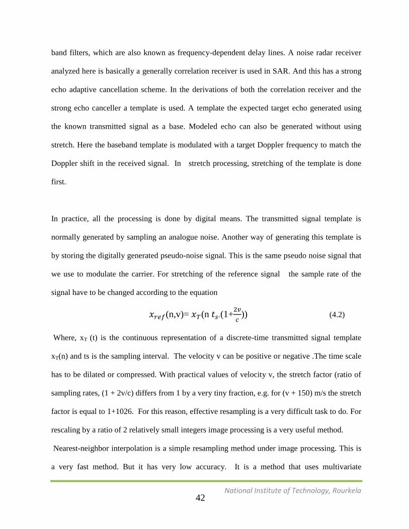
In practice, all the processing is done by digital means. The transmitted signal template is
normally generated by sampling an analogue noise. Another way of generating this template is
by storing the digitally generated pseudo-noise signal. This is the same pseudo noise signal that
we use to modulate the carrier. For stretching of the reference signal the sample rate of the
signal have to be changed according to the equation
(n,v)= (n (1+
)) (4.2)
Where, xT (t) is the continuous representation of a discrete-time transmitted signal template
xT(n) and ts is the sampling interval. The velocity v can be positive or negative .The time scale
has to be dilated or compressed. With practical values of velocity v, the stretch factor (ratio of
sampling rates, (1 + 2v/c) differs from 1 by a very tiny fraction, e.g. for (v + 150) m/s the stretch
factor is equal to 1+1026. For this reason, effective resampling is a very difficult task to do. For
rescaling by a ratio of 2 relatively small integers image processing is a very useful method.
Nearest-neighbor interpolation is a simple resampling method under image processing. This is
a very fast method. But it has very low accuracy. It is a method that uses multivariate
42
National Institute of Technology, Rourkela
interpolation single or multiple dimensions. Its algorithm is such that, it only chose the value of
particular nearest point. Values of the neighboring points ignored. As a result, a piecewise
constant interpolant is obtained. For stretch factor very close to 1, periodic removal of one out
of c/2v samples is done.
4.3 Various Methods in Stretch Processing to remove Masking Effect
4.3.1: Linear interpolation method
Here linear combinations of adjacent original samples are considered for calculating the new
samples. It can be considered as a method of curve fitting using the linear polynomials.
(n,v)= (⌊ (1+
) ⌋)+ (1- )(⌊ (1+
) ⌋) (4.3)
4.3.2 Poly-phase Method
Here upsampling by an integer factor N and then downsampling by another factor M are done.
Polyphase filtering method use low-pass filters to remove aliasing. Aliasing is the effect that
causes various signals to become indistinguishable when sampled. In a standard application, a
rational M/N stretch factor is generated by linear filter with M coefficient sets, changing for
each output sample. In the stretch processing as the M/N is equal to a number very close to 1.
The number of coefficient sets in stretch processing used to be very large. So it is tried to
achieve a smaller number of coefficient sets. Here a polyphase resampler is used to evaluate
sample values for time instants from a set of points. These points are oversampled by a certain
integer factor.
Then the most exact value at the desired point between the available samples is sorted out by
applying linear interpolation method.
43
National Institute of Technology, Rourkela
4.3.3 Chirp-z transforms
It is an efficient method to compute the z-transform on a set of points that are defined as a
where n =N0 ... N1. We first set,
a = exp (j2p (1+2v/c)/N (4.4)
And then calculation of the chirp-z transform of an N-point FFT is done. After that we
effectively obtain the signal resampled with an accurate required rate. But chirp-z transform is a
very complex method than the FFT. Its efficient implementation is very difficult to achieve.
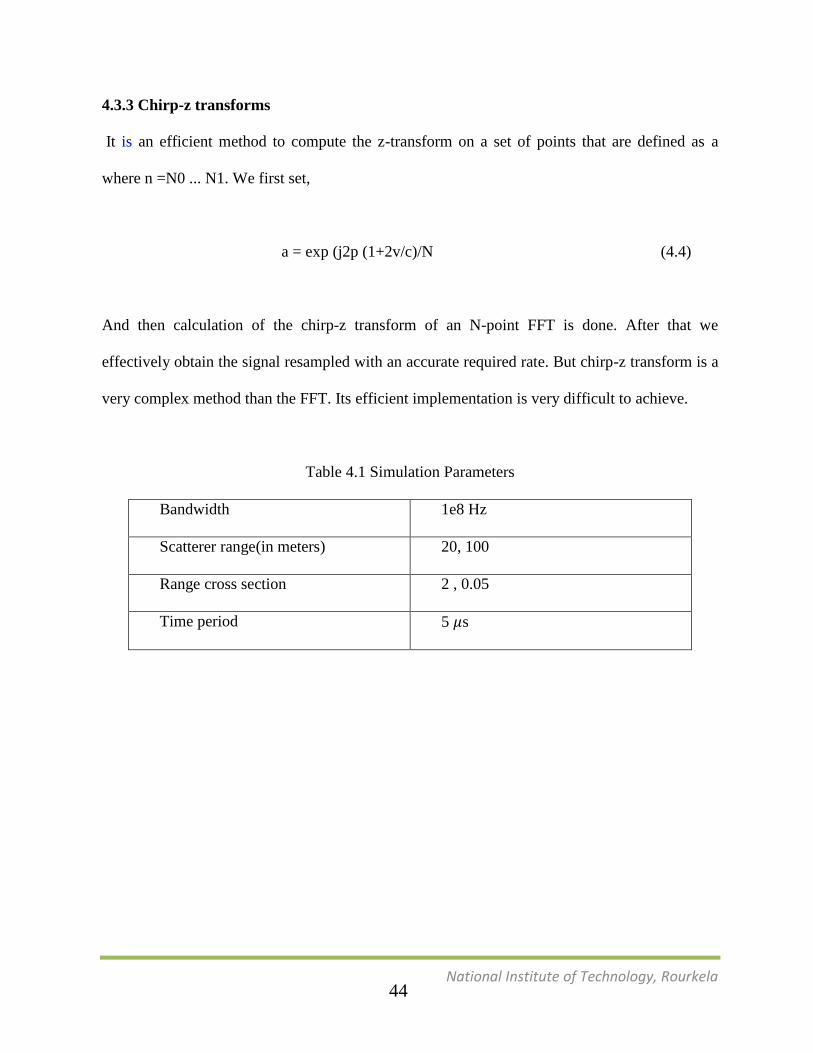
Table 4.1 Simulation Parameters
Bandwidth 1e8 Hz
Scatterer range(in meters) 20, 100
Range cross section 2 , 0.05
Time period 5 s
44
National Institute of Technology, Rourkela
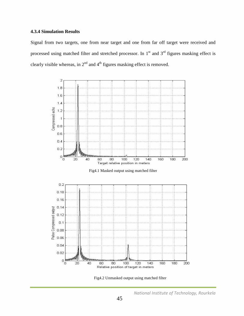
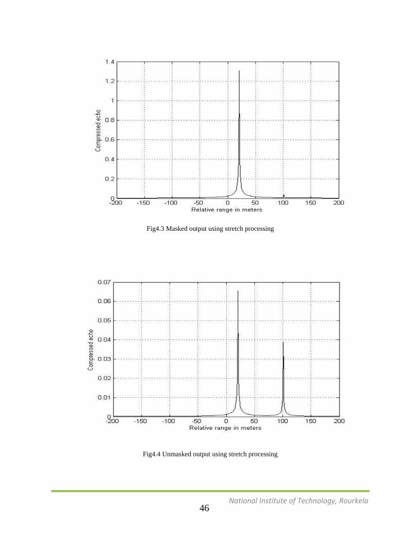
4.3.4 Simulation Results
Signal from two targets, one from near target and one from far off target were received and
processed using matched filter and stretched processor. In 1st and 3
rd figures masking effect is
clearly visible whereas, in 2nd
and 4th
figures masking effect is removed.
Fig4.1 Masked output using matched filter
Fig4.2 Unmasked output using matched filter
45
National Institute of Technology, Rourkela
Fig4.3 Masked output using stretch processing
Fig4.4 Unmasked output using stretch processing
46

National Institute of Technology, Rourkela
4.4 Conclusion
Masking effect is a common problem radar signal processing in which a nearby target masks or
hides echos coming from a far target. In this chapter we have tried to remove the masking effect
on far off target by simply by subtracting echo of nearby target from the received signal. The
two methods described in chapter 2:-.Matched filtering and Stretch processing were used to
process the signals. It is found out that stretch processing has better masking effect removal than
match filtering process
47
National Institute of Technology, Rourkela
CHAPTER 5 CONCLUSION
In pulse compression for correlation of received signal with replica of transmitted signal
matched filtering preferred while dealing with narrowband signals and stretch process is
preferred while dealing with wideband signal. It is also concluded that stretch processing is a
better technique when range resolution is taken into account i.e. Stretch processing method
gives better range resolution than match filtering technique. Stretch processor also has better
side lobe cancellation than match filter method and it does quicker processing than matched
filtering.
LFM signals when passed through 8 different windows:
1. Hanning window 5. Blackmanharris window
2. Hamming window 6. Nuttal window
3. Kaiser window 7. Flattop window
4. Rectangular window 8. Triangular window
Best side lobe cancellation effect is shown by Blackmanharris window. PSR of LFM signals
using different windows, increases with increase in time band width product and decreases with
increase in Doppler shift.
Masking effect is a common problem radar signal processing in which a nearby target masks or
hides echoes coming from a far target. We have tried to remove the masking effect on far off
target due to a nearby target simply by subtracting echo of nearby target from the received
signal. The two methods used were. Matched filtering and Stretch processing .It was found out
that stretch processing has better masking effect removal than match filtering process
48
National Institute of Technology, Rourkela
REFERENCE
[1] Mahafza R. Bassem, Radar Systems Analysis and Design using MATLAB, 2nd
Ed.Ch.5,
7, New York: Chapman & Hall/CRC
[2] Ozdemir Caner, Inverse Synthetic Aperture Radar Imaging with MATLAB Algorithms,
Ch.3, New Jersey: John Wiley & Sons.
[3] David K.Barton, Radar System Analysis and Modeling, Ch.5 and 8, Norwood: Artech
House.
[4] Sahoo A.K. (2012). Development of Radar Pulse Compression Techniques Using
Computational Intelligence Tools. Ph.D. Thesis. NIT Rourkela.
[5] Schlutz M. (2009). Synthetic Aperture Radar Imaging Simulated in MATLAB.
M.S.Thesis.: California Polytechnic State University.
[6] Kulpa K., Misiurewicz J.: ‘Stretch processing for long integration time passive covert
radar’. Proc. 2006 CIE Int. Conf. Radar, Shanghai, China, 2006, pp. 496–499 Cao
[7] Yunhe, Zhang Shouhong, Wang Hongxian, Gao Zhaozhao.: ‘Wideband Adaptive
Sidelobe Cancellation Based on Stretch processing’, Signal Processing, 2006 8th
International Conference Vol.1, 2006
[8] Torres J A, Davis R M, J D R Kramer, et al. “Efficient wideband jammer nulling when
using stretch processing”, IEEE Tran AES. 36(4): 1167-1178, 2000.
[9]. Misiurewicz J. Kulpa K.: ‘Stretch processing for masking effect removal in noise radar’,
IET Proc. , Radar Sonar Navig., 2008, Vol. 2, No. 4, pp. 274–283
49

National Institute of Technology, Rourkela
[10] Torres Jose A, Davis Richard M, Kramer J. Davis R., Fante Ronald L.: ‘Efficient
Wideband Jammer Nulling When Using Stretch Processing’, IEEE Proc. ,Transactions On
Aerospace and electronics systems Vol. 36, No. 4 October 2000.
50