Quantum Mechanics interpreted in Quantum Real Numbers.

John V Corbett∗ and Thomas Durt†

()

ABSTRACT

The concept of number is fundamental to the formulation of any physical theory. We givea heuristic motivation for the reformulation of Quantum Mechanics in terms of non-standardreal numbers called Quantum Real Numbers. The standard axioms of quantum mechanicsare re-interpreted. Our aim is to show that, when formulated in the language of quantumreal numbers, the laws of quantum mechanics appear more natural, less counterintuitivethan when they are presented in terms of standard numbers.

PACS number(s): 03.65

INTRODUCTION

In both classical and quantum physics,the states of a system are represented by math-ematical entities (points of the phase-space, wave-functions) that ultimately consist of setsof real numbers. These real numbers are either rational or arbitrarily well approximated byrational numbers. The states are assumed to change in time according to infinitely precisenumerical laws, but measurements only determine rational numerical values with finite ac-curacy. Nonetheless, the accurate experimental confirmation of the numerical predictionsof quantum mechanics strongly encourages those who believe in the basic role played bynumbers in our universe and in the potential for human beings to know and understand thelaws that the numbers obey. However we think that the often unstated assumption, ”thatthe elements of calculation are identical with the elements of observation” [13] is wrong.Our model [1] of quantum real numbers abandons this identification. Other abandonmentsare well-known, for example, Heisenberg’s original paper on quantum mechanics denied theassumption on the grounds that only relations ”between observable quantities” [10] can beused. Our model does not adhere to Heisenberg’s requirement, on the contrary, in it physicalquantities take quantum real numbers as their values even when they are not observed. Amore recent model that abandons this identification is the non-commutative geometry [7]model of A. Connes. Compared with it, our model is much less ambitious and requires a lessradical change in the picture of the world because in it the values of physical quantities are

∗Department of Mathematics,Macquarie University, N.S.W. 2109, Australia, Emailaddress:jvc@ics.mq.edu.au

†TENA, TONA Free University of Brussels, Pleinlaan 2, B-1050 Brussels, Belgium Email,address:thomdurt@vub.ac.be.

1

given by (commuting) Dedekind real numbers, constructed as cuts in the rational numbers,even though not all quantum real numbers exist to full extent.

As an example consider the position of a particle in a given state at a given time. Inthe classical description, three real numbers suffice to define the value of the position of aparticle; in quantum mechanics, the position of the particle is represented by a triplet of self-adjoint operators. It usually is not acceptable to describe the particle’s position by a tripletof numerical values when the particle’s state is represented by a wave-function. Howeverit is generally conceded that there is an average value for the position with a probabilitydistribution which is given by the modulus squared of the wavefunction in position space.Thus in the standard quantum mechanical picture a quantum particle is not a material pointbut is associated with a cloud of probabilities which is spread throughout space. Thereforequantum physics seems to be non-local, an impression that has been confirmed, or at leastnot contradicted, by all the experiments on Bell’s inequalities. Besides non-locality, whichis revealed through the EPR paradox, the measurement problem in quantum mechanicsis at the source of several paradoxical situations (the Schrodinger cat and the quantumZeno paradoxes for instance) that clearly illustrate the clash between classical and quantuminterpretations and ontologies.

In our view, understanding of the conceptual differences between classical and quantumphysics is improved by the recognition that there can be different realisations of real numbersdetermined by the different theories1. To return to the position of a particle, in our modelits values are given by a triplet of quantum real numbers, each of which relates, roughlyspeaking, to a standard real number like a continuous function on an interval does to a pointin the interval. We shall give a fuller definition of quantum real numbers later.

We will not develop the quantum real numbers interpretation in a strict axiomatic mannerhere. We start by accepting the standard Hilbert space mathematical structures that areused in quantum theories but we do not accept their standard interpretation.

Schematically, our work is structured as follows: first the quantum real numbers aredefined in basic postulate 0. Then the prototype of a filtering or preparation procedure istaken to be the single slit experiment for the position of a particle. This experiment canbe described classically when the quantum real number associated to the position behavesclassically in passing through the slit. This is taken to mean that the square of this quantumnumber must equal the quantum number associated to the square of the position to withinthe order of a small positive standard real number ε. This situation is called the ε sharpcollimation of the position. If on passing through a slit there is strictly ε sharp collimationfor the particle’s position then Theorem 4 shows that the von Neumann transformation lawholds for changes in the quantum real number values of other quantities, up to the same ε.A type of Heisenberg inequality for the widths of position and momentum slits is obtainedin Theorem 2.

This analysis of the prototype motivates the introduction of the basic postulates of thequantum real number interpretation of quantum mechanics.

1The logic of the non-standard quantum real numbers is intuitionistic [11]. For a discussion ofthis aspect of the theory, and for instance, of the reformulation of classical De Morgan’s rules, see[1]. The formulation of quantum real numbers in terms of sheaves and toposes is given in [2].

2

Basic postulate 1 expresses the condition that the statistics of a quantum experimentfor any quantity is close to deterministic when the experiment supports strictly ε sharpcollimation for the values of that quantity.

Next, we reinterpret, in terms of quantum real numbers, an argument due to Goldstone[9,16] and others to show that the statistics relative to repeated measurements performed onidentically prepared systems always gives the conventional quantum probability rules. Thatis, the Born probability rules [19] hold. The proof of Theorem 5 also assumes basic postu-late 2 which is equivalent to the quantum ergodic hypothesis. These two basic postulatesestablish the probabilistic features of arbitrarily prepared quantum systems.

The basic postulates 3A and 3B express the persistence of measured values, therebyrestricting the range of application of these postulates. The Luders-von Neumann transfor-mation rule follows in Propositions 2 and 3.

The effect of this class of measurements of quantum real numbers is to refine them to bea sharp quantum number which lie in the interval of standard real numbers defined by theresolution of the measuring apparatus. Therefore in this interpretation the state of a systemat a given time can be defined by the set of all the quantum real numbers determined duringthe preparation/measurement process. This corresponds closely to the classical conceptexcept that quantum real numbers are used instead of standard real numbers.

An example of how a combination of unitary, standard, dynamics and the requirementof measured values to be unambiguously registered (revealed) by a classical apparatus forcesthe measured values to be almost classical quantum real numbers is proved in Proposition4.

Next we consider single particle dynamics and the 19th century view that matter iscomposed of atoms obeying Newtonian dynamics is modified in that the values of the physicalquantities are given by quantum real numbers instead of standard real numbers. Basicpostulate 4 asserts that the dynamical equations of motion of a quantum system are given byHamilton/Newton’s equations expressed in quantum real numbers. Theorem 6 then assertsthat Heisenberg’s operator equations of motion when averaged over certain open subsets ofstate space closely approximate the Newtonian equations for quantum real number definedon these open sets. These open sets do not cover state space so that the approximate equalitycannot be extended to the whole of state space.

Finally, we conclude by reformulating some paradoxes in the language of quantum num-bers.

I. QUANTUM NUMBERS-THE ONE SLIT EXPERIMENT.

A. Quantum numbers-the basic postulate 0.

Consider a measurement of position. The passage from one to three dimensions does notbring any new insight into the problem, so that we will consider only the measurement ofone coordinate of position, let us say, the projection of the position along the Z-axis. Ourtreatment is not relativistic so that time will always be treated as an external parameterin the following. The position of a classical particle (material point) along the Z-axis isexpressed by one standard real number: z.

3

Let Σ be the set of all density matrices ρ, where ρ is a positive-definite bounded self-adjoint operator on L2(R) of trace 1. In conventional quantum mechanics, every particularpreparation procedure corresponds to a particular choice or determination of a ρ or of asubset of them. A priori, before we prepare the particle, we may be as ignorant of the statesρ as we are of the values of the position z of the particle. Nevertheless in our model weassume that the particle has a set of states associated with it at all times, even when wedon’t know what they are. Furthermore all measurements of the position z yield standardreal numbers. We take this to mean that while the position is associated with a self-adjointoperator Z on L2(R), its values are given by quantum real numbers of the form zQ(U) with:

zQ(U) = Tr(ρZ); ρ ∈ U, (1)

where U is an open subset of Σ. The open subsets of Σ are defined by the weakest topologythat makes Tr(ρ.M) continuous as a function from Σ to the standard real numbers R for anylinear operator M that is self-adjoint and continuous. Here continuous means either boundedon L2(R) or continuous in the standard countably normed topology on the Schwartz spaceS(R). This topology is studied in [2]; we shall call it the standard topology on Σ. Quantumreal numbers of the form zQ(U) are real numbers in the sense of Dedekind 2 [2].

We assume that preparation processes determine open sets U and not single states ρ.Thus we impose the following definition of quantum number in the form of a postulate:Basic postulate 0:The values of a physical quantity are represented by quantum real numbers of the form

MQ(U) = Tr(ρ.M)ρ ∈ U , where U is an open subset of the set of density matrices Σ, and

M is a self-adjoint, continuous linear operator. Furthermore, every physical quantity has aquantum real number value at all times.

Next we consider what happens when we measure the quantum number ZQ(U) by lettingthe particle pass through a slit. According to de Broglie every measurement is in the lastresort a measurement of position so that this will be a paradigm for the measurement process.

B. The one slit experiment and sharp collimation.

Assume that we can produce particles and prepare them to pass through a rectangularslit in a vertical barrier. We assume that the geometry of the experiment is such that theslit is infinitely extended horizontally. Let us denote by z1 and z2 the Z-coordinates of thelower and upper extremities of the slit.

2Dedekind real numbers are obtained as cuts in the set of rational numbers Q . A cut is a divisionof Q into two classes L and R, with every rational in L less than every rational in R . WhenL does not have a largest member and R does not have a smallest member the cut defines anirrational number. For the quantum real number MQ(U), where U is an open subset of Σ and M

is a self adjoint operator, the cut is defined by sections over subsets Wj of an open cover of U withthe rationals QQ(Wj) given by locally constants functions over W . Locally constant functions areconstant globally only when defined on a connected set [14,17].

4

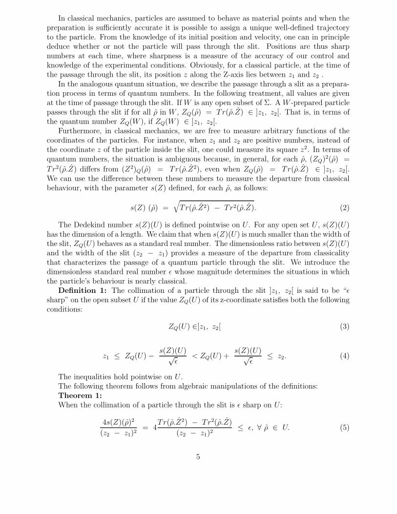
In classical mechanics, particles are assumed to behave as material points and when thepreparation is sufficiently accurate it is possible to assign a unique well-defined trajectoryto the particle. From the knowledge of its initial position and velocity, one can in principlededuce whether or not the particle will pass through the slit. Positions are thus sharpnumbers at each time, where sharpness is a measure of the accuracy of our control andknowledge of the experimental conditions. Obviously, for a classical particle, at the time ofthe passage through the slit, its position z along the Z-axis lies between z1 and z2 .

In the analogous quantum situation, we describe the passage through a slit as a prepara-tion process in terms of quantum numbers. In the following treatment, all values are givenat the time of passage through the slit. If W is any open subset of Σ. A W -prepared particlepasses through the slit if for all ρ in W , ZQ(ρ) = Tr(ρ.Z) ∈ ]z1, z2[. That is, in terms ofthe quantum number ZQ(W ), if ZQ(W ) ∈ ]z1, z2[.

Furthermore, in classical mechanics, we are free to measure arbitrary functions of thecoordinates of the particles. For instance, when z1 and z2 are positive numbers, instead ofthe coordinate z of the particle inside the slit, one could measure its square z2. In terms ofquantum numbers, the situation is ambiguous because, in general, for each ρ, (ZQ)2(ρ) =

Tr2(ρ.Z) differs from (Z2)Q(ρ) = Tr(ρ.Z2), even when ZQ(ρ) = Tr(ρ.Z) ∈ ]z1, z2[.We can use the difference between these numbers to measure the departure from classicalbehaviour, with the parameter s(Z) defined, for each ρ, as follows:

s(Z) (ρ) =√Tr(ρ.Z2) − Tr2(ρ.Z). (2)

The Dedekind number s(Z)(U) is defined pointwise on U . For any open set U , s(Z)(U)has the dimension of a length. We claim that when s(Z)(U) is much smaller than the width ofthe slit, ZQ(U) behaves as a standard real number. The dimensionless ratio between s(Z)(U)and the width of the slit (z2 − z1) provides a measure of the departure from classicalitythat characterizes the passage of a quantum particle through the slit. We introduce thedimensionless standard real number ε whose magnitude determines the situations in whichthe particle’s behaviour is nearly classical.

Definition 1: The collimation of a particle through the slit ]z1, z2[ is said to be “εsharp” on the open subset U if the value ZQ(U) of its z-coordinate satisfies both the followingconditions:

ZQ(U) ∈]z1, z2[ (3)

z1 ≤ ZQ(U)− s(Z)(U)√ε

< ZQ(U) +s(Z)(U)√

ε≤ z2. (4)

The inequalities hold pointwise on U .The following theorem follows from algebraic manipulations of the definitions:Theorem 1:When the collimation of a particle through the slit is ε sharp on U :

4s(Z)(ρ)2

(z2 − z1)2= 4

Tr(ρ.Z2) − Tr2(ρ.Z)

(z2 − z1)2≤ ε, ∀ ρ ∈ U. (5)

5

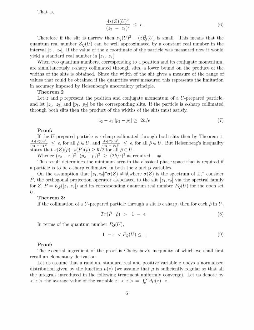
That is,

4s(Z)(U)2

(z2 − z1)2≤ ε. (6)

Therefore if the slit is narrow then zQ(U)2 − (z)2Q(U) is small. This means that the

quantum real number ZQ(U) can be well approximated by a constant real number in theinterval ]z1, z2[. If the value of the z coordinate of the particle was measured now it wouldyield a standard real number in ]z1, z2[

When two quantum numbers, corresponding to a position and its conjugate momentum,are simultaneously ε-sharp collimated through slits, a lower bound on the product of thewidths of the slits is obtained. Since the width of the slit gives a measure of the range ofvalues that could be obtained if the quantities were measured this represents the limitationin accuracy imposed by Heisenberg’s uncertainty principle.

Theorem 2Let z and p represent the position and conjugate momentum of a U-prepared particle,

and let ]z1, z2[ and ]p1, p2[ be the corresponding slits. If the particle is ε-sharp collimatedthrough both slits then the product of the widths of the slits must satisfy,

|z2 − z1||p2 − p1| ≥ 2h/ε (7)

Proof:If the U-prepared particle is ε-sharp collimated through both slits then by Theorem 1,

4s(Z)(ρ)2

(z2 − z1)2≤ ε, for all ρ ∈ U , and 4s(P )(ρ)2

(p2 − p1)2≤ ε, for all ρ ∈ U . But Heisenberg’s inequality

states that s(Z)(ρ) · s(P )(ρ) ≥ h/2 for all ρ ∈ U .Whence (z2 − z1)

2. (p2 − p1)2 ≥ (2h/ε)2 as required. #

This result determines the minimum area in the classical phase space that is required ifa particle is to be ε-sharp collimated in both the z and p variables.

On the assumption that ]z1, z2[∩σ(Z) 6= ∅,where σ(Z) is the spectrum of Z,” considerP , the orthogonal projection operator associated to the slit ]z1, z2[ via the spectral familyfor Z, P = EZ(]z1, z2[) and its corresponding quantum real number PQ(U) for the open setU .

Theorem 3:If the collimation of a U-prepared particle through a slit is ε sharp, then for each ρ in U ,

Tr(P · ρ) > 1 − ε. (8)

In terms of the quantum number PQ(U),

1 − ε < PQ(U) ≤ 1. (9)

Proof:The essential ingredient of the proof is Chebyshev’s inequality of which we shall first

recall an elementary derivation.Let us assume that a random, standard real and positive variable z obeys a normalised

distribution given by the function µ(z) (we assume that µ is sufficiently regular so that allthe integrals introduced in the following treatment uniformly converge). Let us denote by< z > the average value of the variable z: < z > =

∫∞o dµ(z) · z.

6

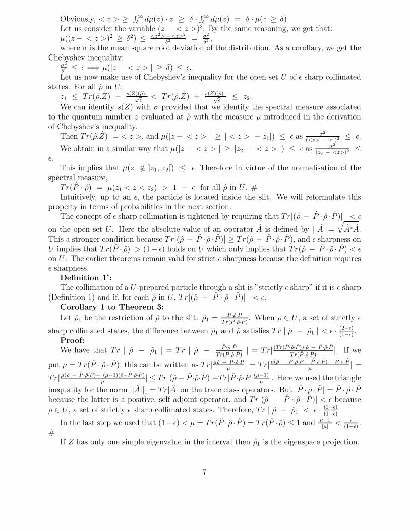
Obviously, < z > ≥ ∫∞δ dµ(z) · z ≥ δ · ∫∞δ dµ(z) = δ · µ(z ≥ δ).

Let us consider the variable (z− < z >)2. By the same reasoning, we get that:µ((z− < z >)2 ≥ δ2) ≤ <z2>−<z>2

δ2 = σ2

δ2 ,where σ is the mean square root deviation of the distribution. As a corollary, we get the

Chebyshev inequality:σ2

δ2 ≤ ε =⇒ µ(|z− < z > | ≥ δ) ≤ ε.Let us now make use of Chebyshev’s inequality for the open set U of ε sharp collimated

states. For all ρ in U :z1 ≤ Tr(ρ.Z) − s(Z)(ρ)√

ε< Tr(ρ.Z) + s(Z)(ρ)√

ε≤ z2.

We can identify s(Z) with σ provided that we identify the spectral measure associatedto the quantum number z evaluated at ρ with the measure µ introduced in the derivationof Chebyshev’s inequality.

Then Tr(ρ.Z) = < z >, and µ(|z− < z > | ≥ | < z > − z1|) ≤ ε as σ2

(<z> − z1)2≤ ε.

We obtain in a similar way that µ(|z− < z > | ≥ |z2 − < z > |) ≤ ε as σ2

(z2 − <z>)2≤

ε.This implies that µ(z /∈ ]z1, z2[) ≤ ε. Therefore in virtue of the normalisation of the

spectral measure,Tr(P · ρ) = µ(z1 < z < z2) > 1 − ε for all ρ in U . #Intuitively, up to an ε, the particle is located inside the slit. We will reformulate this

property in terms of probabilities in the next section.The concept of ε sharp collimation is tightened by requiring that Tr|(ρ − P · ρ · P )| | < ε

on the open set U . Here the absolute value of an operator A is defined by | A |=√A∗A.

This a stronger condition because Tr|(ρ − P · ρ · P )| ≥ Tr(ρ − P · ρ · P ), and ε sharpness onU implies that Tr(P · ρ) > (1− ε) holds on U which only implies that Tr(ρ − P · ρ · P ) < εon U . The earlier theorems remain valid for strict ε sharpness because the definition requiresε sharpness.

Definition 1’:The collimation of a U -prepared particle through a slit is ”strictly ε sharp” if it is ε sharp

(Definition 1) and if, for each ρ in U , Tr|(ρ − P · ρ · P )| | < ε.Corollary 1 to Theorem 3:

Let ρ1 be the restriction of ρ to the slit: ρ1 = P ·ρ·PT r(P ·ρ·P )

. When ρ ∈ U , a set of strictly ε

sharp collimated states, the difference between ρ1 and ρ satisfies Tr | ρ − ρ1 | < ε · (2−ε)(1−ε)

.Proof:We have that Tr | ρ − ρ1 | = Tr | ρ − P ·ρ·P

T r(P ·ρ·P )| = Tr| (Tr(P ·ρ·P ))·ρ − P ·ρ·P

T r(P ·ρ·P )|. If we

put µ = Tr(P · ρ · P ), this can be written as Tr|µρ − P ·ρ·Pµ

| = Tr|µ(ρ − P ·ρ·P+ P ·ρ·P )− P ·ρ·Pµ

| =

Tr|µ(ρ − P ·ρ·P )+ (µ−1)(ρ−P ·ρ·P )µ

| ≤ Tr|(ρ− P ·ρ·P )|+Tr|P ·ρ·P | (µ−1)µ

. Here we used the triangle

inequality for the norm ||A||1 = Tr|A| on the trace class operators. But |P · ρ · P | = P · ρ · Pbecause the latter is a positive, self adjoint operator, and Tr|(ρ − P · ρ · P )| < ε because

ρ ∈ U , a set of strictly ε sharp collimated states. Therefore, Tr | ρ − ρ1 |< ε · (2−ε)(1−ε)

In the last step we used that (1−ε) < µ = Tr(P · ρ · P ) = Tr(P · ρ) ≤ 1 and |µ−1||µ| < ε

(1−ε).

#If Z has only one simple eigenvalue in the interval then ρ1 is the eigenspace projection.

7

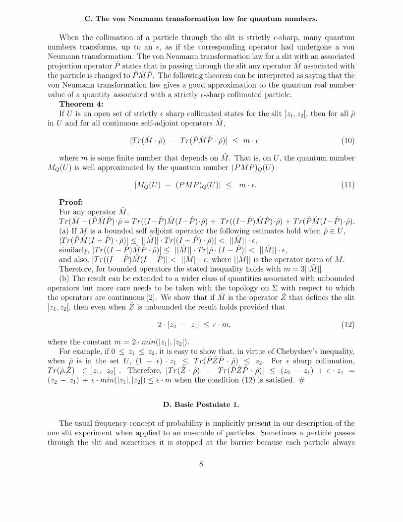
C. The von Neumann transformation law for quantum numbers.

When the collimation of a particle through the slit is strictly ε-sharp, many quantumnumbers transforms, up to an ε, as if the corresponding operator had undergone a vonNeumann transformation. The von Neumann transformation law for a slit with an associatedprojection operator P states that in passing through the slit any operator M associated withthe particle is changed to P M P . The following theorem can be interpreted as saying that thevon Neumann transformation law gives a good approximation to the quantum real numbervalue of a quantity associated with a strictly ε-sharp collimated particle.

Theorem 4:If U is an open set of strictly ε sharp collimated states for the slit ]z1, z2[, then for all ρ

in U and for all continuous self-adjoint operators M ,

|Tr(M · ρ) − Tr(P M P · ρ)| ≤ m · ε (10)

where m is some finite number that depends on M . That is, on U , the quantum numberMQ(U) is well approximated by the quantum number (PMP )Q(U)

|MQ(U) − (PMP )Q(U)| ≤ m · ε. (11)

Proof:For any operator M ,Tr(M −(P MP )·ρ= Tr((I−P )M(I−P )·ρ) + Tr((I−P )MP )·ρ) + Tr(P M(I−P )·ρ).(a) If M is a bounded self adjoint operator the following estimates hold when ρ ∈ U ,|Tr(P M(I − P ) · ρ)| ≤ ||M || · Tr|(I − P ) · ρ)| < ||M || · ε,similarly, |Tr((I − P )MP · ρ)| ≤ ||M || · Tr|ρ · (I − P )| < ||M || · ε,and also, |Tr((I − P )M(I − P )| < ||M || · ε, where ||M || is the operator norm of M .Therefore, for bounded operators the stated inequality holds with m = 3||M ||.(b) The result can be extended to a wider class of quantities associated with unbounded

operators but more care needs to be taken with the topology on Σ with respect to whichthe operators are continuous [2]. We show that if M is the operator Z that defines the slit]z1, z2[, then even when Z is unbounded the result holds provided that

2 · |z2 − z1| ≤ ε ·m, (12)

where the constant m = 2 ·min(|z1|, |z2|).For example, if 0 ≤ z1 ≤ z2, it is easy to show that, in virtue of Chebyshev’s inequality,

when ρ is in the set U , (1 − ε) · z1 ≤ Tr(P ZP · ρ) ≤ z2. For ε sharp collimation,Tr(ρ.Z) ∈ ]z1, z2[ . Therefore, |Tr(Z · ρ) − Tr(P ZP · ρ)| ≤ (z2 − z1) + ε · z1 =(z2 − z1) + ε ·min(|z1|, |z2|) ≤ ε ·m when the condition (12) is satisfied. #

D. Basic Postulate 1.

The usual frequency concept of probability is implicitly present in our description of theone slit experiment when applied to an ensemble of particles. Sometimes a particle passesthrough the slit and sometimes it is stopped at the barrier because each particle always

8

has a position given by a quantum real number. When the U-prepared particles are allε sharp collimated and if ε approaches zero then s(Z)(U) becomes infinitely smaller thanthe extension of the slit so the quantum particle should behave like a pointlike particle andpass through the slit with probability one. That is, ε sharp collimated quantum numbersapproximate, to within ε, standard classical numbers in the spectrum of the self-adjointoperator associated with the quantity being collimated. This suggests that the measurablevalues of a quantum number must belong to the spectrum of the self-adjoint operator.

These considerations recall the philosophy of Niels Bohr in which the measurement pro-cess gives an interface between the classical and quantum worlds. In this interface quantumpotentialities become actual, a process sometimes called the objectification process. In termsof quantum real numbers, it is a process in which the quantum real numbers become sharpand realise standard, classical values.

Basic Postulate 1:(i) The measured values of physical quantities always belong to the spectrum of the

corresponding self-adjoint operator. (ii) If a quantity is associated with the self-adjointoperator M and if U is an open subset of strictly ε sharp collimated states for the interval]m1, m2[ in the spectrum of M , then the probability that the quantum number MQ(U)belongs to ]m1, m2[ is larger than 1− ε.

Note that by Theorem 3, if P = EM(]m1, m2[) is the projection operator for the interval]m1, m2[ then we can identify PQ(U) > 1− ε as the probability of passing through the slitwhen U is an open subset of strongly ε sharp collimated states for the interval.

There is a special case, when the associated operator M has only one eigenvalue λ in]m1, m2[ so that P is the projection onto the eigenspace for λ and if U is an open set ofstrongly ε sharp collimated states for ]m1, m2[, then the probability that MQ(U) = λ isPQ(U) > 1− ε.

Except in the special case described above there will be many different standard realnumbers in the interval that could be realised as the measured value of of the quantity. Ina measurement the quantum real number value MQ(U) of the quantity is forced to realiseone of them. We do not know with what probability the different sharp values will occur.Basic postulate 1 gives an estimation of the probability of passage through the slit only inthe nearly deterministic regime, i.e., in situations of sharp collimation. In the next sectionwe start to evaluate the probabilities of getting different outcomes in simple cases.

II. DEDUCTION OF THE QUANTUM PROBABILITY LAW.

In the standard quantum mechanics literature the question of whether quantum prob-ability rules like Born’s should be postulated independently has been discussed. Severalattempts to derive the quantum probability rule by considering many copies of a systemand postulating the validity of the eigenstate rule have been made [16]. The eigenstate rulestates that if the system was prepared in an eigenstate of a self-adjoint operator A then anysubsequent measurement of A always yields the corresponding eigenvalue.

The eigenstate rule is not equivalent to our first basic postulate. Nevertheless, our firstbasic postulate implies an modified version of the eigenstate rule in the special case when Ahas only one eigenvalue λ in the interval ]a1, a2[.

9

If we are content with equality up to an ε we can show that the basic postulate 1 impliesBorn’s rule. We shall only sketch the proof in the case of the simplest quantum experiment,a dichotomic experiment, following the treatment given by Goldstone [9] and modified bySquires [16]. A general proof of a similar result was obtained by Busch for observables witha continuous spectrum [6].

We require another postulate, the ”ergodic assumption”Basic Postulate 2 The result of an average measurement performed at the same time

on N identical copies of a system and the averaged result of N individual measurementsperformed successively in time on N identically prepared systems are identically distributed.

Theorem 5: If basic postulates 1 and 2 are satisfied, and the system is prepared in anneighbourhood W of the density matrix ρ0, W = ρ|Tr|(ρ − ρ0)| < ε then, up to ε,the probability of measuring the outcome i, for i = 1, 0, equals Trρ0P (i), where P (1) is theprojection operator of the slit and P (0) = 1 − P (1). That is,

|PQ(i)(W ) − Tr(ρ0P (i))| < ε. (13)

Proof:Following the notation introduced by Squires [16], we define an “average” operator Q

constructed to give the average value of a dichotomic quantity, with values 1 or 0, associatedto the passage through the slit. On account of this choice of values for the quantity, theaverage value can be identified with the relative frequency of passage through the slit.

Q = 1N

∑i: 1...N Qi(1), where Qi(1) =

⊗I1

⊗....

⊗Pi(1)

⊗...

⊗IN , an N-fold tensor

product with the identity operator in each slot except the ith which contains Pi(1). It iseasy to check that the spectrum of Q goes from 0 to 1 by steps 1

N. This is due to the fact

that the spectrum of each projector Pi(1) is equal to 0, 1.We consider N identical copies of the density matrix state ρ0, Ω0 =

⊗Nj=1 ρ0(j), of each

state ρ ∈W , Ω =⊗N

j=1 ρ(j) and of the open set W , W =∏N

j=1W (j).

Now Tr(Ω0 · Q) = Tr(ρ0 · P (1)), 6= 0 by assumption, Tr(Ω · Q) = Tr(ρ · P (1)) and henceQQ(W ) = P (1)Q(W ) = p(W ).

Now consider the N-particle projection operators that are a tensor product of J “yes”single particle projections , Pi(1), and (N − J) “no” single particle projections, Pi(0). Bypermuting the order of the single particle operators we deduce that for each J there are(

NJ

)= N !

J ! (N − J)!such N-particle operators which represent N-particle measurements in

which J particles do, and (N − J) do not, pass through the slit. For any of these N-particleprojections QJ and any ρ ∈ W ,

Tr(ρ · QJ) = (Tr(ρ · P (1)))J (Tr(ρ · P (0)))(N−J).Therefore if prepared in the open set W the quantum real number associated to the

situation in which J particles do and (N−J) don’t pass through the slit is(

NJ

)·(P (1)Q(W ))J

(P (0)Q(W ))(N−J).Now, this is just the expression for the probability of having J favourable and N − J

unfavourable events in a Bernouilli process with probabilities (P (1)Q(W )) and (P (0)Q(W )).This is only a formal identification but the expression can be manipulated mathematically.

In the limit as N goes to infinity the Bernouilli (binomial) distribution can be approxi-mated by a Gaussian distribution:(

NJ

)· p(W )J q(W )N − J ∼ 1√

2π N p(W ) q(W )·exp−(J −Np(W ))2

2 N p(W ) q(W ).

10

Also, the spectrum of Q tends to cover the unit interval in this limit and this Gaussiandistribution scales to a normal density function for the relative frequency x = J/N givenby ψ(x) = (2πp(W )q(W )/N)−1/2 · exp − [(x − p(W ))2/(2p(W )q(W )/N)]. Therefore ψ hasmean < x >= p(W ) and standard deviation (p(W )q(W )/N)1/2.

In virtue of Chebyshev’s inequality, µ(|x− < x > | ≥ δ) ≤ (p(W )q(W )/N)δ2 .

Therefore, since ψ(x) is the probability density function for the relative frequency x,µ(|x− < x > | ≥ δ) = 1 − ∫ <x>+δ

<x>−δ ψ(x)dx . On using δ = 1√N1 − λ

, with λ a positivestandard real number between 0 and 1, the probability of the frequency lying in the interval[p(W ) − 1√

N1−λ, p(W ) + 1√

N1−λ] is larger than 1 - p(W )·q(W )

Nλ which shows how the relative

frequency approaches p(W ) in the large N limit.Suppose that we measure the relative frequency, represented by Q, with a measuring

device of resolution 2R, which means that we are unable to distinguish values that are lessthan a distance 2R apart. For any realistic device, R can be assumed to be a very smallstandard real number but is never equal to zero. By choosing N sufficiently large, we canalways ensure that the standard deviation S(Q)(W ) = (p(W )q(W )/N)1/2 is much smaller

than the resolution 2R of the apparatus. Actually, whenever N is larger than p(W )·q(W )ε·R2

and then W is a set of ε sharp collimated states for the slit ]p(W ) − R, p(W ) + R[ formeasuring Q. Therefore by basic postulate 1,for systems prepared in W the probability thatwe observe values of QQ(W ) that belong to the interval ]p(W ) − R, p(W ) + R[ is 1 towithin an ε. This means that, with probability 1 up to an ε, the result of the measurementof Q will be equal to p(W ) to within the resolution 2R of the apparatus.

Now, by basic postulate 2, the averaged result of N individual dichotomic measurementsperformed successively on N identically prepared systems in the open set W and the resultsof an average measurement of Q performed at the same time on N identical copies of asystem in the open set W are equally distributed. Since the result of measuring Q is almostcertainly p(W ) in the sense made precise before, we have that in the limit of large N theaverage value of the individual operator Pi(1) is certainly equal to p(W ). This averagevalue obtained after N individual measurements is precisely the frequency or probability ofobtaining the result ”yes” in an individual measurement.

Finally we must show that this result holds uniformly over W . Each density matrix ρin W satisfies Tr|(ρ − ρ0)| < ε. But, for i = 0, 1,P (i) is a bounded operator of norm 1,therefore, |Tr(ρP (i)) − Tr(ρ0P (i))| < ε.

That is, for each i = 1, 0, the probability of measuring the outcome i is essentiallyconstant, up to an ε, and equal to Tr(ρ0P (i)) for all density matrices in the neighbourhoodW . In terms of the quantum numbers P (i)Q(W ),i = 1, 0, |P (i)Q(W )− γ(i)| < ε where the

standard real number γ(i) = Tr(ρ0P (i)).This completes the proof that the basic postulates 1 and 2 are sufficient to derive Born’s

quantum probability rule because when P (1)) projects onto the 1 dimensional space spannedby |1〉 and the state ρ0 is pure and equals |ψ〉〈ψ| where ψ is a unit vector then Tr(ρ0P (1))equals the Born rule expression, | 〈ψ|1〉 |2. #

The generalisation of this argument to a finite sequence of dichotomic observations andthus to an arbitrary discretised measurement process is straightforward. If any realisticexperiment can only have a finite number of outcomes then we have established the frequencymeaning of probability for realistic experiments. We have still to develop dynamical modelsof how the different outcomes are realised.

11

It is easy to show that, in virtue of the Theorems 3 and 5, when the collimation of aparticle through the slit is ε sharp, the particle will pass through the slit with probabilityequal to 1 (up to an ε). This shows the internal consistency of our choice of axioms.

III. PERSISTENCE OF MEASURED VALUES.

Let us return to the single slit experiment as the prototype of a class of measurementsin which the measured values persist. In order to guarantee the persistence of the observedvalues of the positions of the particle, we must impose the following continuity condition:immediately after the particle has passed through the slit, the probability is negligible offinding it elsewhere than in the vicinity of the slit. That is, there exists a standard realnumber 0 < ε << 1 and an open set U such that for each ρ in U ,

Tr(P · ρ) > 1 − ε, (14)

P being the spectral projection for the slit.Basic Postulate 3 A:If a quantity A is measured and found to have values in the subset I, then there exists a

standard real number 0 < ε << 1 such that immediately after the measurement, the systembelongs to the largest open set U on which Tr|(I − P ) · ρ| < ε, P being the spectralprojector of A onto I.

Consequently, in terms of the quantum number PQ(U),

1 − ε < PQ(U) ≤ 1. (15)

Proposition 1:When the basic postulates 1, 2 and 3 A are satisfied, if a subset I of values of a quantity

is measured, then, just after the measurement, the quantum numerical value of the quantitywill still belong to I with probability close to one.

Proof:Let A denote the self-adjoint operator of to the quantity being measured and let us

assume that the measured values belong to the subset I. The basic postulate 3 A impliesthat, if P is the spectral projection operator for A on the subset I, then immediately after themeasurement the system is in the set U on which 1 − ε < PQ(U) ≤ 1. By a straightforwardapplication of the Born rule, the validity of which was established in theorem 5, this meansthat the probability that the quantum number AR(U) belongs to I is greater than 1 − ε.#

We further note that in the limit of vanishing ε, any bounded observable B transformsaccording to the von Neumann transformation rule on the open set U because for ρ ∈ U ,

| Tr(ρ · B) − Tr(ρ · P BP ) | ≤ ||B|| · ε.The proof of this result is the same as that of Theorem 4 which dealt with the case of

strictly ε sharp collimated states.Comment:The persistence/continuity in time of the quantum real number values of the particle’s

position was implicitly assumed when we described a passage of a particle through a slit inthe first section. The persistence, up to an ε, of the measured values of a particle’s positionis based upon experimental facts, exhibited in the setting up of sources and targets and in

12

bubble chamber pictures when one sees a temporal sequence of aligned excitations, whichapproximate, up to an ε, classical continuous trajectories that exhibit the persistence oflocalisation.

A. The preparation process as a filtering process.

Note that basic postulate 3A is necessary in order to establish the relevance of basicpostulate 1 and of Theorem 5. In order that a state is ε sharp collimated, the particlemust be physically prepared. Similar preparation of N copies of an open set W is neededin the derivation of the theorem 5. This can be done, in principle, using a combination ofdynamical evolutions (that we shall describe in a next section) and filtering processes.

Suppose that during the preparation process different quantities are measured succes-sively. It is well-known that if the quantities are represented by commuting operators, theBirkhoff-von Neumann lattice of physical properties admits a classical (Boolean) represen-tation [5]; this suggests that classical logic describes the logic of the outcomes (up to ε). Inthe standard theory this Boolean representation does not exist for quantities representedby non-commuting operators because the distributivity property of the lattice is violated[5]. A similar conclusion is obtained in axiomatic probability theory, the violation of Bell’sinequalities can be shown to reflect the non-existence of a classical probabilistic structureunderlying quantum probability [12]. However in the quantum real number model the logicis intuitionistic [1]. If the outcomes of the measurements are given by quantum real numbervalues then, as Theorem 2 shows, if limited accuracy is accepted, quantities represented bynon-commuting operators can be measured in succession. The logic of propositions is thenintuitionistic but not Boolean in general.To ensure that Boolean logic holds more conditionshave to be imposed on the measurements. We will not pursue this discussion further inthis paper. Nevertheless, for the registered outcomes of measurements, classical, Booleanlogic and probability rules are relevant. Note that, in last resort, it is only through thedevelopment of dynamical models of the measurement process that it ought to be possibleto connect the quantum and the classical worlds.

In standard quantum mechanics, when observables commute, the temporal order in whichthey are measured does not affect the statistical distribution of the outcomes3.Therefore, theoutcome observed during the measurement of a quantum number AQ should persist when

another number BQ is measured provided A and B commute. This discussion is encapsulatedin the following postulate:

Basic Postulate 3 B:

3For instance, it can be shown that when the system is an entangled bipartite system of which thecomponents belong to regions of space-time separated by a Minkoskian spacelike vector, the quan-tum statistical correlations between both systems are the same as when these regions are separatedby a timelike vector. In the latter case, the chronology of the measurements is invariant undera Lorentz transformation. Otherwise, the temporal order depends on which inertial referential ischosen in order to describe the experiment [18].

13

Suppose one quantity is measured and found to have values in the subset I and directlyafterwards a second quantity is measured. If the quantities are represented by stronglycommuting operators A and B and if P is the spectral projector of A onto I, then, just afterthe measurement of B, the system still belongs to the open set U on which Tr|(I−P )·ρ| < ε.Moreover, the temporal order in which A and B are measured does not affect the statisticaldistribution of the outcomes.

Note that an alternative approach was proposed elsewhere [3] in order to describe thejoint-measurement of the observables A and B, that is known in the litterature as thestatistical interpretation. The basic idea is that, being considered that the temporal orderingof the measurement of A and B does not matter, it is sufficient to consider the globalmeasurement as a whole and to apply the Born rule without considering the possibility ofthe collapse of the wave function during partial measurements. Logically, this is a consistentapproach but according to us it does not answer to the question of the collapse of the full wavefunction during the global measurement. It also does not explain why regitered outcomes arepersistent. The concept of persistence introduced by us in the previous postulates reflects ourpersonal philosophical preference according to which a measurement is a real process. Bothviews are consistent, exactly in the same way that the violation of local realism by quantumentangled systems can be interpreted as the refutation either of realism or of locality.

Consequence of the Basic Postulates 3 A and B:If a subset I of values of a quantity A is measured, and that, directly afterwards, a subset

J of values of a quantity B is measured, and that A and B strongly commute, then, justafter the measurement of B, the system will belong to an open neighbourhood U ∩ V , withU = ρ : Tr|(I − P ) · ρ| < ε and V = ρ : Tr|(I − P ′) · ρ| < ε where P is the spectralprojector of A onto I and P ′ is the spectral projector of B onto J .

From the standard quantum mechanics viewpoint,this looks like the conjunction of propo-sitions being represented, in Boolean logic, by the intersection of the characteristic sets ofthe propositions4. However the sets are open, because the logic is intuitionistic [1].

As a consequence of postulates 3 A and 3B, we can use the language of quantum numbersto describe preparation processes as sequences of filtering processes performed on a particle.The prepared state of the particle is then defined by the set of intervals of quantum realnumerical values of the filtered quantities. A new concept of quantum state is derived fromthis set of intervals. Instead of claiming that a certain state, represented by a density matrix,was prepared, we say that the system underwent a preparation procedure during whichcertain quantum numbers were prepared. This provides us with an operational definition ofthe state of a quantum system in terms of quantum numbers.

The equivalence between preparation and measurement for the class of processes in whichmeasured values persist allows the passage from the standard interpretation of quantum

4This analogy with classical logics in the case of commuting observables is also valid for whatconcerns the logical implication, which corresponds to the set-theoretical inclusion relation inBoolean representations. For instance, it is easy to deduce from the definition 1 that, when asystem is ε sharp collimated relatively to a slit of breadth z2 − z1, it will certainly (up to an ε)pass through a parallel and non-distant larger slit of breadth z2 − z1 (with z2 − z1 > z2 − z1)the center of which is aligned with the center of the first slit.

14

theory to that of quantum real numbers in which physical quantities always have quantumnumerical values that exist to extents given by open subsets of Σ. However it is only whenthe measured quantum real numbers approximate standard real numbers closely, that is,when they are ε sharp collimated, and persist, that they become concrete, recordable facts.

The fact that the observed outcomes of a measurement persist makes it possible todefine more accurately the transformation undergone by the quantum real numbers duringthe measurement process.

B. The Luders-von Neumann transformation rule.

In the standard quantum theory, the collapse hypothesis is often given as an independentpostulate governing the behaviour of systems under measurement. It states that if thesystem was prepared as the density matrix ρ0,then during the measurement ρ0 ”collapses”

to ρ′0 = P ·ρ0·PT r(P ·ρ0)

, where P is the projection operator of the slit. Then any observable B

transforms, in the Heisenberg picture, according to the Luders-von Neumann transformation

rule, in which B is changed to P ·B·PT r(P ·ρ0)

.

This transformation rule differs from the von Neumann rule which says that in similarcircumstances B is changed to P · B · P . The difference is due to the fact that for thevon Neumann transformation the preparation of the initial state of the particle includesthe process of collimation through the slit, while the preparation of the initial state for theLuders-von Neumann transformation does not. This distinction is emphasised in the twonext propositions.

Proposition 2 ( Luders-von Neumann rule)Assume that a system is initially prepared in the open set W of states centered on the

state ρ0: W = ρ ∈ Σ : Tr|(ρ − ρ0)| < δ. Next assume that during the preparation ofthe initial state the quantity A is measured/prepared with values in the interval I. Then anyquantity associated with a bounded self-adjoint operatorB has a quantum real number value

given approximately by the constant standard real number Trρ′0 · B, where ρ′0 = P ·ρ0·PT r(ρ0·P )

.

Here P is the spectral projection operator for A on the interval I and P · ρ0 6= 0. Theapproximation is governed by the preparation parameter δ and the persistence parameter ε.

Proof:After the measurement of the quantity A, the system belongs to an open set U defined

in the basic postulate 3 A, on which Tr|(I − P ) · ρ| < ε, where P is the spectral projectionof A onto I. By assumption, the initial preparation is also described by the open set W sothat for any ρ ∈W ∩ U ,

Tr|(ρ− ρ′0)| = Tr|(ρ− ρ0 + ρ0 − ρ′0)| ≤ Tr|(ρ− ρ0)|+ Tr|(ρ0 − ρ′0)| (16)

The first term is less than δ because ρ ∈W .The second is less than ε · (2− ε)/(1− ε) by Corollary 1 to Theorem 3 (the proof of which

is still valid under the present assumptions).Thus

Tr|(ρ− ρ′0)| < δ + ε · (2− ε)/(1− ε). (17)

15

Therefore if ε and δ are small enough the measured value of the quantity with boundedoperator B will be given to a good approximation by the constant number Trρ′0 · B, aspredicted by the Luders-von Neumann transformation. #

Note that in the previous proposition, we assumed that a particular value of the firstquantity A was measured during the preparation process. The next proposition establishesthe Luders-von Neumann rule when the preparation process is assumed to end before themeasurement of the first quantity A.

Proposition 3 (extended Luders-von Neumann rule)Suppose the system has been prepared initially in an open set W of extension ε around

the density matrix ρ0. If A is then measured, found to have values in the interval I(i),i =1, ...., N ,and if Pi, the spectral projection of A for I(i), satisfies Pi · ρ0 6= 0, then immediatelyafter the measurement, the system will belong to an open set W ′(i) of extension ε around

the density matrix ρ′0(i) = Pi·ρ0·Pi

Tr(Pi·ρ0).

Accordingly, the quantum real number associated to any bounded self-adjoint operatorB that strongly commutes with A transforms as follows: BQ(W )−− > BQ(W ′(i))

Proof of the Proposition 3.Consider two strongly commuting self-adjoint operators A and B. To simplify the no-

tation, we suppose that both operators are bounded and that A = ΣNi=1 ai · Pi where

ai ∈ R, N < ∞, and Pi is the projection onto the eigenvalue ai. Given postulate 3 B theoutcomes of measurements performed on A persist during measurements of B when A andB commute so that we can decompose the measurement of A · B into the measurement ofA alone followed by the measurement of B. In virtue of the last part of the postulate 3 B,the probabilistic predictions that we derive from the Born rule will be the same whether wemeasure the quantity A · B as a single quantity or we measure A and B sequentially.

Let the open set W = ρ ∈ Σ : Tr|ρ − ρ0| < ε be given, where ρ0 satisfies

ρ0 · Pi 6= 0, (18)

for each Pi in the spectral decomposition of A.For any ρ ∈ W ,

Tr(ρ · A · B) = Tr(ρ · ΣNi=1 ai · Pi · B) = ΣN

i=1 ai · Tr(ρ · Pi · B) (19)

But

|Tr(ρ · Pi · B)− Tr(ρ · Pi · B · Pi)| = 0. (20)

because A and B strongly commute, so that

|Tr(ρ · A · B)− ΣNi=1 ai · Tr(ρ · Pi · B · Pi)| = 0 (21)

Now since ρ0 was chosen so that Pi · ρ0 6= 0 for any i,

ΣNi=1 ai · Tr(ρ · Pi · B · Pi) = ΣN

i=1 ai · Tr(ρ0 · Pi) · Tr(ρ · Pi · B · Pi)

Tr(ρ0 · Pi)(22)

for all ρ ∈ W . By Theorem 5, for all ρ ∈ W , Tr|(ρ · Pi) − (ρ0 · Pi)| < ε so that|Tr(ρ · Pi · B · Pi) − Tr(ρ0 · Pi · B · Pi)| < ε · ||B||. Thus to within an error that goes to 0

with ε, for all ρ ∈ W , Tr(ρ · A · B) = ΣNi=1 ai · Tr(ρ0 · Pi) · Tr(ρ0·Pi·B·Pi)

Tr(ρ0·Pi).

16

Theorem 5 permits us to approximate the term Tr(ρ0 · Pi) by (Pi)Q(W ). We now use the

permutation property of the trace to rewrite Tr(ρ0·Pi·B·Pi)

Tr(ρ0·Pi)= Trρ′0(i)·B, where ρ′0(i) = Pi·ρ0·Pi

Tr(ρ0·Pi)

is the Luders-von Neumann transformed of ρ0 when the outcome ai has been measured.Thus,for all ρ ∈ W , Tr(ρ · A · B) is well approximated by a sum that is independent of ρ ∈ W .By basic postulate 3B the statistical distribution of the outcomes ai · bj is independent ofwhether the quantities of A and B were measured simultaneously or sequentially.

This result can be written in terms of quantum numbers, if W = ρ;Tr|ρ−ρ0| < ε and

W ′(i) = ρ;Tr|ρ− ρ′0(i)| < ε where ρ′0(i) = Pi·ρ0·Pi

Tr(Pi·ρ0),then

(A · B)Q(W ) ≈ ΣNi=1AQ(W ′(i)) · (Pi)Q(W )BQ(W ′(i)) (23)

That is, the value of (A · B)Q at W equals the sum over i of the products of the valuesof AQ and BQ at W ′(i) weighted by the probability (Pi)Q at W to an approximation thatdepends on the precision of the initial preparation. Note that this result is valid in general,even when Pi · ρ0 = 0 for some i. #

Remark:In the quantum numbers interpretation, we claim on the basis of the results of the previ-

ous subsection that if the measurement of the quantum number AQ involves filtering through

a slit I(i) then any quantity whose corresponding operator commutes with A behaves, up toan ε, as if it had undergone a Luders-von Neumann transformation. Note that this does notimply that the collapse process really occurs, but rather that the collapse postulate gives agood approximation to the quantum numbers obtained in this type of measurement. Nev-ertheless, the change undergone during the measurement process cannot be described solelyby a unitary evolution (this is the core of the so-called measurement problem) as shows thefollowing example.

C. An example of measurement of position

The following example shows that when a particle is sharply localised in space, and thata pointer interacts with this particle according to a well chosen interaction (in this case animpulsive von Neumann interaction Hamiltonian), the pointer reveals unambiguously theposition of the particle. In this example, the apparatus being located in classical space timecan only register (reveal) unambiguously numbers that are approximately classical.

Assume that the system is represented by particle 1, the measuring apparatus by particle2. They will be treated as quantum systems with associated Hibert spaces H(∞) and H(∈),while the combined two particle system has the tensor product Hilbert space H(∞,∈) =H(∞)⊗H(∈). The corresponding state spaces are Σ(1), Σ(2) and Σ(1, 2). When W (1) isan open set in Σ(1) and W (2) is open in Σ(2), we define the superset W (1, 2) of W (1) andW (2) to be the smallest open set in Σ(1, 2) such the partial traces TrH(∞)ρ(1, 2) ∈ W (2)and TrH(∈)ρ(1, 2) ∈W (1) for all ρ(1, 2) ∈W (1, 2).

Initially particle 1 is prepared so that the quantum real number value of its position isX(1)Q(W (1)) where W (1) ⊃ U(1) ∪ V (1). The open sets U(1) and V (1) are such that thequantum real number values X(1)Q(U(1)) and X(1)Q(V (1)) of the particle’s position makeit ε sharp collimated in one of the two slits in the screen. If the slits are determined by the

17

classical numbers a < b < c < d as I1 =]a, b[ and I2 =]c, d[ then a < X(1)Q(U(1)) < b < c <

X(1)Q(V (1)) < d. Clearly U(1) ∩ V (1) = ∅. Let P1 and P2 be the projection operators forthe slits I1 and I2.

Particle 2 is prepared with position X(2)Q(W (2)) which is classical or approximatelyclassical,

[SX(2)(W (2))]2 = |(X(2)Q(W (2)))2 − (X(2)2)Q(W (2))| < ε2, (24)

where ε2 is a very small positive standard real.Now particles 1 and 2 interact through an impulsive von Neumann interaction Hamil-

tonian H(1, 2)Q(U(1, 2)) = g · [X(1) · P(∈)]Q(U(∞,∈)) defined on the open subset U(1, 2)

of Σ(1, 2). Here P(∈) is the self adjoint operator for the momentum of particle 2, X(1) isthat for the position of particle 1 and g is the coupling constant that is such that g · ∆tis finite for the infinitesimal period, ∆t, during which the force acts. The solution of theHamiltonian equations of motion for this Hamiltonian reveals that when the interaction hasceased the position of particle 2 has changed by an amount g · ∆t · X(1)Q(O), where O isan open subset of Σ(1).

Proposition 4The final position of particle 2 is approximately classical if O is either an open subset

of U(1) or an open subset of V (1) such that X(1)Q(O) is almost classical. However, ifO = U(1) ∪ V (1) then the final position of particle 2 is not approximately classical whichmeans that when particle 1’s quantum position covers both slits it is not registered by themeasurement particle 2.

Proof:The final position of particle 2 is X(2)Q(W (2)) + g · ∆t · X(1)(O) which we will call

X(2)f , the corresponding operator is X(2)f = I(1) ⊗ X(2) + g · ∆t X(1) ⊗ I(2) and letO(1, 2) be the super set of W (2) and O.

Start by assuming that O = U(1) is such that X(1)Q(U(1)) is approximately classical,then [SX(2)f

(O(1, 2))]2 = [SX(2)(W (2))]2+

(g ·∆t)2[SX(1)(U(1))]2 +2g ·∆t(−X(1)Q(U(1)) ·X(2)Q(W (2))+(X(1)⊗ X(2))(O(1, 2))).The right hand side is small if both X(2)Q(W (2)) and X(1)Q(U(1)) are approxi-

mately classical, since the first two terms are, by definition, and the third term is alsosmall because approximately classical quantum numbers are approximately homothetic,i.e.,X(2)Q(W (2)) ≈ x2IQ(W (2)) and X(1)Q(U(1)) ≈ x1IQ(U(1)) where x1 and x2 are standardreal numbers.

The same argument works if U(1) replaces V (1). Similar arguments work when,forexample, X(1)Q(W (1)) is not approximately classical but there is an open set O ⊂ W (1)so that X(1)Q(O) is. However the argument does not work when O = U(1) ∪ V (1) becausein that case X(1)Q(O) is not approximately classical, i.e., [SX(1)(O)]2 is not small. If a

measurement of position would occur, then, according to the basic postulate 3 A, X(2)f

ought to become concentrated around the value that gets registered during the process and[SX(2)f

(O(1, 2))]2 would then be small. Therefore no persistent registration is likely to occurwhen O = U(1) ∪ V (1). Note that a similar result occurs if O is centered around say afifty-fifty coherent superposition of states that belong to U(1) and V (1). #

This model result implies that the quantum particle 1 may pass through both slits si-multaneously but such events are not unambiguously revealed (or persistently registered)

18

by the measurement particle 2 because then the position of particle 2 is not even approxi-mately classical. Nevertheless, this example shows that it is not impossible to reintroduce inthe quantum numbers approach the counterpart of classical objectivity provided somewhereinside the chain of measurements that separates the quantum system and the observer, adevice is classical, so to say, a quantity A is measured and found to have (persistent) valuesin the subset I. The question to know precisely at which level of the chain such a classicalmeasurement apparatus is present is in last resort a question of personal interpretation. If Ican be considered to be a sharp subset, relatively to subsequent measurement devices similarto the one described in the previous section, all of them will reveal unambiguously valuescontained inside I and their result will be consistent with those associated to A.

What we cannot explain at this level, and this is the deep mystery of quantum me-chanics, the essence of the yet unsolved measurement problem, is how quantum numbersbecome sharp. This objectification process, or ”collapse” process ought in principle to bedue simply to the interaction between the system and the measurement apparatus but sucha process, during which superpositions are broken is not consistent with the unitarity ofHeisenberg-Schrodinger evolution as we have shown. This point will be briefly discussed inthe conclusions.

At least, the measurment problem suggests that it is worth investigating non-standard(non-unitary) dynmical laws. This will be done in the next section, where we propose(speculatively) a new type of dynamics. We shall assume that quantum particles obey thesimplest generalisation of classical dynamics that can be derived on the assumption thatquantities take quantum real number values.

IV. QUANTUM DYNAMICS WITH QUANTUM REAL NUMBERS.

In the first section, we introduced sharply collimated particles as a heuristic examplewhich helped to motivate the choice of the basic postulates 1 and 2. These particles canbe considered to be classical in the sense that they behave like localised pointlike particleswith regard to passing or not through a slit. In this section, open subsets of Σ containingsharply collimated particles are used to show that the unitary quantum mechanical evolu-tion laws give good approximations to quasi-classical dynamical laws expressed in quantumreal numbers. The set Σ of density matrices is restricted so that the unbounded positionand momentum operators, Qj and Pj , of the Schrodinger representation of the canonicalcommutation relations give quantum real numbers as continuous functions on Σ [2].

Basic Postulate 4 (tentative)Consider the example of a non-relativistic quantum particle of positive mass µ that moves

in a central force field F which is derived from a potential function V . We assume that thequantum values (Qj)Q of the position coordinates and (Pj)Q of the conjugate momenta ofthe particle globally satisfy equations of motion that resemble the equations of classical me-chanics. That is, the global quantum numbers (Qj)Q and (Pj)Q satisfy Hamilton’s equations.

Thus, µd(Qj)Q(U)

dt= (Pj)Q(U) and

d(Pj)Q(U)

dt= Fj( ~QQ(U)) hold for all open subsets U ∈ Σ,

where ddt

denotes differentiation with respect to time, Fj represents the the jth componentof the force. Fj is the jth component of the negative gradient, −∇V , of the scalar potential

function V ( ~QQ) where ~QQ = ((Q1)Q, (Q2)Q, (Q3)Q)).

19

This means that for all ρ ∈ Σ, µdTr(Qj ρ)

dt= Tr(Pjρ) and

dTr(Pj ρ)

dt= Fj(Tr(Qρ))

We will sometimes use Newton’s equations which are, in terms of the (Qj)Q(Σ),

µd2((Qj)Q(Σ))

dt2= Fj(QQ(Σ)). Again this means that for all ρ ∈ Σ, µ

d2(Tr(Qj ρ)

dt2) = Fj(Tr(Qρ)).

An inverse to Ehrenfest’s TheoremWe will now prove a theorem that states that if basic postulate 4 holds then the self-

adjoint operators Qj and Pj satisfy equations that well approximate Heisenberg’s operatorequations of motion when localised to certain open subsets of Σ. To simplify the notationwe will assume that the particle is one dimensional.

The theorem relates a set of operator equations, Heisenberg’s equations, to a set of quan-tum real number equations, Newton’s equations so we have first to explain what approximateequality between them means. A straightforward way to get a quantum real number equa-tion from an operator equation is to multiply each side of the operator equation by a densityoperator, ρ, and then take the trace of each side. The original operator equation becomes afamily of numerical equations which can be localised in an open subset of Σ by restrictingthe ρ’s to belong to the subset.

Recall that Heisenberg’s equations for an operator A aredAdt

= −i[A, H ]

where H is the Hamiltonian operator of the system and the square bracket denotes theoperator commutator. For the one dimensional motion, the Hamiltonian operator is

H = 1(2µ)

P 2 + V (Q).To simplify the discussion we remove the explicit dependence of the equations on the

momentum operator P and just use Newton’s equations of motion in the form of secondorder differential equations. If Newton’s quantum real number equations hold to the extentW , then for all ρ in W ,

µ d2(Tr(Qρ)dt2

) = F (TrρQ).If Heisenberg’s numerical equations hold to the extent W , then for all ρ in W

µ d2(Tr(Qρ)dt2

) = TrρF (Q).The difference between the right hand sides of these equations shows why Ehrenfest’s

Theorem is not valid for all functions F . In general,TrρF (Q) 6= F (TrρQ). Note that in principle this difference is experimentally testable,

which shows that the quantum real number approach to quantum mechanics is not purelyad hoc.

It is possible, however, that the difference between the two sides is small at some stateρa and remains small in an open neighborhood of ρa. Then the equations are approximatelyequal on that open set. This will be taken to mean that Heisenberg’s numerical equationsgive a good approximation to Newton’s equation in that neighbourhood. We claim that fora suitable class of functions F , this is true in the vicinity of every point on the position lineof the one dimensional model. That is, for every standard real number r and standard realnumber ε > 0, we can find an open set, W (r, ε) in Σ, such that, both

(a) the quantum real number QQ(W (r, ε)) is arbitrarily close to r, and

(b)for each ρ in W (r, ε), TrρF (Q) is arbitrarily close to F (TrρQ).The physical interpretation is that if an observer’s measurement apparatus is located in

the immediate vicinity of the position r then the observer cannot measure any significantdifference between the accelerations of the particle due to the two forces, TrρF (Q) and

20

F (TrρQ). The unitary evolution of quantum mechanics gives a local linear approximationto the equations of classical mechanics expressed in quantum real numbers.

The class of suitable functions is defined through the concept of S-continuity.Definition 3:A function F is S-continuous, if it is real-valued continuous functions of a real variable

such that, for the position operator Q, F (Q) defines an operator on the Schwartz space Sthat is continuous in the standard countably normed topology on S.

The class of S-continuous functions includes all polynomials [2].Theorem 6:If the force F is S-continuous, then given ε > 0, Heisenberg’s equations of motion

approximate Newton’s equations of motion to within ε on each member of a collection ofopen sets W (r, ε) of Σ, indexed by the standard real numbers r and ε. That is, for all ρ inW (r, ε),

|TrρF (Q)− F (TrρQ)| < ε.Proof:The idea behind the proof is to find states ρr at which F (TrρrQ) closely approximates

TrρrF (Q), then F (TrρQ) will be close to TrρF (Q) for all ρ that are such that both F (TrρQ)is close to F (TrρrQ) and TrρF (Q) is close to TrρrF (Q). To achieve this we must firstconstruct the open sets W (r, ε).

Definition 4:Given F ,r and ε, W (r, ε) = N(ρr, Q, δ) ∩ N(ρr, F (Q), ε

3), where, δ is given by |F (r) −

F (x)| < ε6

if |r − x| < δ (δ depends upon both ε and r) and ρr satisfies both |TrρrF (Q)−F (r)| < ε

6and |TrρrQ− r| < δ

2.

That such density operators ρr exist follows from Weyl’s criterion [15].Lemma 1:If Q is a self-adjoint operator which has absolutely continuous spectrum, then for any

real number r in its spectrum we can construct a sequence of pure states ρn such that, forthe given S-continuous function F , TrρnF (Q) approaches F (r) and TrρnQ approaches r,as n approaches infinity.

Proof:From Weyl’s criterion [15] it follows that, for any number r in the spectrum of Q, there

exists a sequence of unit vectors un, in the domain of Q, such that if ρn is the projectiononto the one dimensional subspace spanned by the vector un then TrρnQ approaches r asn→∞.

The vectors un can be chosen to be in S. Furthermore we can find a sequence ofvectors un ∈ S such that for n large enough the support of un lies in a narrow intervalcentred on r. Then, the corresponding one dimensional projection operators (ρn), are suchthat the sequence of standard real numbers TrρnF (Q) approaches F (r) by S-continuity, andthe sequence of standard real numbers TrρnQ approaches r by the spectral theorem for Q.#

From Lemma 1, once we are given a real number r in the spectrum of Q, the S-continuousfunction F and a real number ε > 0, we can find an integer N such that, for all j > N , both|TrρjF (Q)− F (r)| < ε

6and |TrρjQ− r| < δ

2where δ is given in Definition 4.

We choose ρr =ρj, for some j > N , and deduce that

|TrρrF (Q)− F (TrρrQ)| < ε3

21

because|TrρrF (Q)− F (TrρrQ)|≤ |TrρrF (Q)− F (r)| + |F (r)− F (TrρrQ)|.With this choice of ρr, the construction of the open set W (r, ε) is completed.Proof of Theorem 6, (continued):For all ρ ∈W (r, ε) we have|TrρF (Q)− F (TrρQ)|≤ |TrρF (Q)− TrρrF (Q)| + |TrρrF (Q)− F (TrρrQ)| + |F (TrρrQ)− F (TrρQ)|.If ρ is in N(ρr, F (Q), ε

3) the first summand is < ε

3, as is the second by choice of ρr. The

final summand is also < ε3

because

|F (TrρrQ)− F (TrρQ)| ≤ |F (TrρrQ)− F (r)|+ |F (r)− F (TrρQ)|.Here the first summand is < ε

6by the definition of ρr in Definition 4. Furthermore,the

second summand is < ε6

because the function F is continuous at r and with x = TrρQ,

|x− r| ≤ |x − TrρrQ| + |TrρrQ− r| < δ2

+ δ2

= δ, because ρ ∈ W (r, ε), and because of thechoice of ρr in Definition 4.

Therefore, for any ρ in W (r, ε), |TrρF (Q)− F (TrρQ)| < ε. #The question remains whether we can construct sufficiently many of these open sets. In

general, for a given S-smooth function F , the family of open sets W (r, ε), does not forman open cover of the state space Σ. The physically important exception is the linear forcelaw,eg simple harmonic motion, when equality holds for all ρ in Σ.

However, for every permissible F , the family of open sets W (r, ε) covers the classicalcoordinate space of the physical system in the sense that associated with each W (r, ε) thereis an open interval (r − δ, r + δ), with δ defined in Definition 4,such that the collection ofthese intervals covers the standard real line which is the classical coordinate space of thismodel.

If we had used three dimensions for the classical configuration space of the particle, theanalog of Theorem 6 would permit us to deduce that there is a family of open sets W (~x, ε),with ~x ∈ R3,on which Heisenberg’s numerical equations give a good approximation toNewton’s equation. Furthermore associated to each W (~x, ε) is an open ball B(~x, δ) in R3,the collection of which cover R3. Again an observer measuring a particle with apparatusset up in one of these open balls could not determine locally whether the evolution of theparticle was governed by Heisenberg’s equations of motion averaged over a ρ from W (~x, ε)

or by Newtons equations of motion for the quantum numbers ~Q |W restricted to W (~x, ε).It is interesting to see how these results correlate with the ideas of collimation of a

particle. Take the open interval (z1, z2) = (r − δ, r + δ) to be the slit through which theparticle is ε sharp collimated. Let U be such that for all ρ ∈ U , the particle is ε-sharpcollimated, if δ < m · ε, where m = 2 ·min(|z1|, |z2|) (see Theorem 4) and Q is taken to beZ then W (r, ε) is contained in U , to an extent that depends on the force F .

V. CONCLUSIONS AND REMARKS.

A. Some remarks.

a) The importance of continuity.

22

It is worth noting that continuity is the basic property that allows a physical theory toremain valid under slight changes (up to an ε) and even to be persistent in the presence ofprofound reformulations. In our approach, continuity was present at all levels: the deductionof the form of the unitary evolution laws and of the quantum probability rule are based ona requirement of continuity between the classical and the quantum regimes (the law oflarge numbers itself presupposes some kind of continuity). The basic postulate 3 reflects atthe quantum level the classical properties of continuity in time of the physical magnitudes(persistence). The central role played by continuity is too often neglected or ignored inquantum mechanics. Our formulation in terms of quantum numbers helps to restore thecentrality of the role played by continuity in quantum mechanics.

b) About quantum paradoxes.Let us now quickly look at three celebrated paradoxes, the EPR, the Schrodinger cat

and the quantum Zeno paradoxes using the language of quantum real numbers.Provided we think in terms of quantum real numbers, the values taken by physical

properties can always be expressed as quantum numbers and only in extreme circumstances,such as an ε sharp collimation, are well-approximated by standard real numbers. So wemust abandon that part of our classical intuition according to which the values of quantitiespreexist as standard real numbers before the measurement. They only pre-exist as quantumreal numbers. In our model different classical standard real number values of position canbe determined by measurements on a single particle with a single quantum real numbervalue for its position. Therefore the usual concept of localisation which refers to classicalstandard real number values of position needs to be reviewed in the light of the particlehaving quantum real values for its position. The particle may be localised in terms ofthe quantum real number values of its position but not localised in terms of the classicalstandard real number values of its position. We plan to examine the Einstein- Podolsky-Rosen paradox in detail in a future work.

A cat composed of atoms and molecules which may be localised in terms of quantum realnumber values but not localised in terms of classical standard real number values could aswell be both living and dead to an observer if the difference between being alive and beingdead is just a question of molecular configurations. In the standard theories of quantummechanics there remains the basic problem of the quantum theory of measurement: toprecisely determine the border-line that separates a measurement regime from a regime ofunitary evolution. What is it that actualises potentialities? Our model provides a differentway of posing the question. Do there exist Newtonian forces that when expressed in quantumreal numbers allow a quantity whose quantum real number values are not ε sharp collimatedto evolve so that its quantum real number values do become ε sharp collimated? It seemsreasonable that such forces exist, but we do not yet have an answer to this question. Note

that an equation of the kind µ d(Tr(Qρ)dt

) = λ · (Tr2ρQ − TrρQ2) (with λ taken to be apositive real) makes it possible to describe the measurement (sharpening) of the observableQ. However, such an evolution is nor an Hamiltonian evolution (because it introduces anarrow of time) neither a Newtonian one because it does not contain any acceleration term. Itis certainly not a Schrodingerlike, unitary, evolution because it is not linear in ρ. Neverthelessit is expressed solely in terms of quantum real numbers.

The quantum Zeno paradox is based on the assumptions that in a measurement thewave function collapses and that the collapse process is instantaneous. Firstly, it is worth

23

noting that if a chain of measuring devices is present between the observed quantum systemand the human observer, as is always the case, it is clear that the measurement process isnot instantaneous, a point that was made clear through our analysis of the impulsive vonNeumann interaction. Beside, as we have suggested following our analysis of the proposition4, there ought to exist dynamical forces that link the quantum real number values of physicalquantities to classical values of quantities associated with the measurement apparatus andthereby cause the quantum real number values to become ε sharp. Such forces could be usedto model measurement processes to give a quasi-dynamical description of the ”collapse” inwhich there will be no Zeno paradox. Moreover it can be shown that, in virtue of the lawof large numbers, when the number of particles of the system under observation increases,the effect of the collapse process decreases proportionnally because the Hilbertian distancebetween the initial state and the collapsed state decreases when N increases. Then, providedthe measurement time τ is very small but not negligibly small, the change imposed during atime T by a series of T

τsuccessive measurements will become negligible in the limit of large

numbers. This property is an extension of the results derived in the section 2. We plan toexamine it in detail in a future work.

This section has not provided hard solutions to the paradoxes of quantum mechanics butit does outline some projects of using quantum real numbers to study and perhaps resolvethem.

B. Conclusions.

In order to clarify the correspondences between conventional quantum mechanics and thequantum numbers approach,we will compare the standard axioms of quantum mechanics asthey are enumerated in the text-book of Cohen-tannoudji et al. [4] and our basic postulates:

Standard Axioms 1, 2 and 3: 1; states are represented by rays of the Hilbert space orconvex combinations of them (density matrices), 2; measurable quantities are represented byself-adjoint operators (observables) and 3; measurable values are eigenvalues of these opera-tors (in other words, observed physical quantities belong to the spectrum of the observableunder measurement).

Basic postulate 1; Physical quantities always have numerical values as quantum realnumbers of the form MQ(U) = Tr(ρ.M)ρ ∈ U where U is an open subset of the set of

density matrices Σ, and M is a self-adjoint, continuous linear operator.Any system alwayshas an open set of states associated with it. The measured values of a physical quantityalways belong to the spectrum of the corresponding self-adjoint operator.

The standard axiom 4 in ref. [4] is the Born rule.The Born rule is a consequence of the basic postulate 1 and basic postulate 2, the

ergodicity assumption.The standard axiom 5 [4] is the collapse hypothesis.The collapse hypothesis, in the form of the Luders-von Neumann transformation rule (so

to say in its weakest form), is a consequence of the Born rule and of our postulates 3 A and3 B, which characterize the persistence in time of observed outcomes.

The standard axiom 6 [4] assumes that the time evolution is given by the Schrodingerequation or equivalently the Heisenberg equations for the observables.

24

In a dynamical model of the measurement of the position of a particle we showed howthe quantum real number value of the position is forced to be an almost classical realnumber if we impose that it gets registered during a unitary interaction with the classicalmeasurement apparatus, which suggests that new, non-unitray dynamics ought to be studiedin the framework of the quantum real number interpretation of quantum mechanics.

Basic postulate 4 states that the position and momentum of a particle when expressedin quantum real numbers satisfy Hamiltonian/Newtonian equations of motion. Theorem 6shows that for a certain class of forces, there are open sets of state space on which Heisen-berg’s equations of motion give close approximations to Newton’s equation of motion inquantum real numbers. Furthermore while this class of open sets doesn’t cover state space,it does cover the classical position space of the particle. Thus at every point in positionspace we cannot distinguish locally between the two types of dynamical motion.

We hope that the quantum real number interpretation of quantum mechanics will openthe way for a deeper understanding.

ACKNOWLEDGMENTS

T.D. is a Postdoctoral Fellow of the Fonds voor Wetenschappelijke Onderzoek, Vlaan-deren.

25

REFERENCES

[1] M.Adelman and J. V. Corbett: ”A Sheaf Model for Intuitionistic Quantum Mechanics”,Applied Categorical Structures 3 79-104 (1995)

[2] M.Adelman and J.V. Corbett: ”Quantum Mechanics as an Intuitionistic form of Clas-sical Mechanics” to appear in Proceedings of the Centre Mathematics and its Applica-tions, ANU, Canberra (2001).

[3] L. E. Ballentine: “Limitations of the projection postulate”, Founds. Phys. 20 n 3(1990) 1329.

[4] C. Cohen-Tannoudji, B. Diu and F. Laloe, Mecanique quantique, (Hermann, Paris,1977).

[5] G. Birkhoff and J. von Neumann: “The logic of quantum mechanics”, Annals of Math-ematics 37 (1936) 823.

[6] P. Busch and P. Lahti: “Individual aspects of quantum measurements” J. Phys. A:Math.Gen. 29 (1996)

[7] A. Connes, Geometrie Non-Commutative, (InterEditions,Paris, 1990).

[8] C. Dewndney, P.R. Holland, A. Kyprianidis and J.P. Vigier: “Spin and non-locality inquantum mechanics”, Nature 336 n6199 (1988) 536

[9] E. Farhi, J. Goldstone and S. Gutmann: “How probability arises in quantum mechanics”Ann. Phys. (NY)192 (1989).

[10] W. Heisenberg, Zs.Phys.33 (1925) pp879-893, translated in B. L. van der Waerden,Sources of Quantum Mechanics, pp261-276 (Dover, 1968).

[11] A. Heyting: “Intuitionism, an introduction” eds. North Holland, Amsterdam.(1971).

[12] D. Gutkoski and G. Masotto “An inequality stronger than Bell’s inequality”, Nuov.Cim., 22 B, n1, (1974).

[13] R. B. Lindsay and H. Margenau, Foundations of Physics, p397 (Dover, 1957).

[14] S. MacLane and I. Moerdijk, Sheaves in Geometry and Logic (Springer–Verlag, NewYork, 1994).

[15] W. Reed and B. Simon, Methods of Mathematical Physics I: Functional Analysis (Aca-demic Press, New York, 1972).

[16] J. Squires: “On an alleged “proof” of the quantum probability law” Phys. Lett. A145n23 (1990).

[17] L. N. Stout, Cahiers Top. et Geom. Diff. XVII, 295 (1976); C. Mulvey, “IntuitionisticAlgebra and Representation of Rings” in Memoirs of the AMS 148 (1974).

[18] W. Tittel, J. Brendel, H. Zbinden and N. Gisin: “Long-distance Bell-type tests usingenergy-time entangled photons”, Phys. Rev. A 59 (1999) 4150.

[19] J. V. von Neumann: “Mathematische grundlagen der quanten-mechanik”, Springer-Verlag, Berlin (1932).

26