Quantum Mechanics || Dynamical Symmetries

14. Dynamical Symmetries

We have seen in the preceding chapters that the symmetry and degeneracy of the states of a system are associated with each other. For example, a system that possesses rotational symmetry is usually degenerate with respect to the direction of the angular momentum, i.e. with respect to the eigenvalues of a particular component (usually J z). An exception is the case J = O. In the case of the discrete symmetries of space-inversion and time-reversal discussed in the previous chapter, degeneracy is less common since the transformed states are quite frequently equal to the original states.

Subsequently we will see in more detail that beyond the degeneracies arising, say, in rotational symmetry there is the possibility of degeneracies of different origin. Such degeneracies are to be expected whenever the Schrodinger equation can be solved in more than one way, either in different coordinate systems, or in a single coordinate system which can be oriented in different directions. From our present considerations we should expect these degeneracies to be associated with some symmetry, too. These symmetries differ essentially from all the others considered so far, because their nature is not geometrical. They are called dynamical symmetries, since they are the consequence of particular forms of the Schrodinger equation or of the classical force law. We shall examine two relatively simple quantum mechanical examples which, starting from the corresponding classical systems, allow the derivation of the existence and then the general form of the dynamical symmetry in very nearly the same way as for geometrical symmetries. Of course this is not possible in general; indeed many quantum mechanical systems have no classical analogue.

14.1 The Hydrogen Atom

First we investigate the classical Kepler problem. In relative coordinates the Hamiltonian is given by

(14.1)

Here Il is the reduced mass of the system and K is a positive quantity (for the hydrogen atom K = Ze2). The bound solutions of the classical problem are ellipses, and the distance from perihelion P to aphelion A is called 2a. If b denotes the length of the minor semiaxis, the eccentricity e is e = (a 2 - b2)1/2 fa

W. Greiner et al., Quantum Mechanics© Springer-Verlag Berlin Heidelberg 1994

454

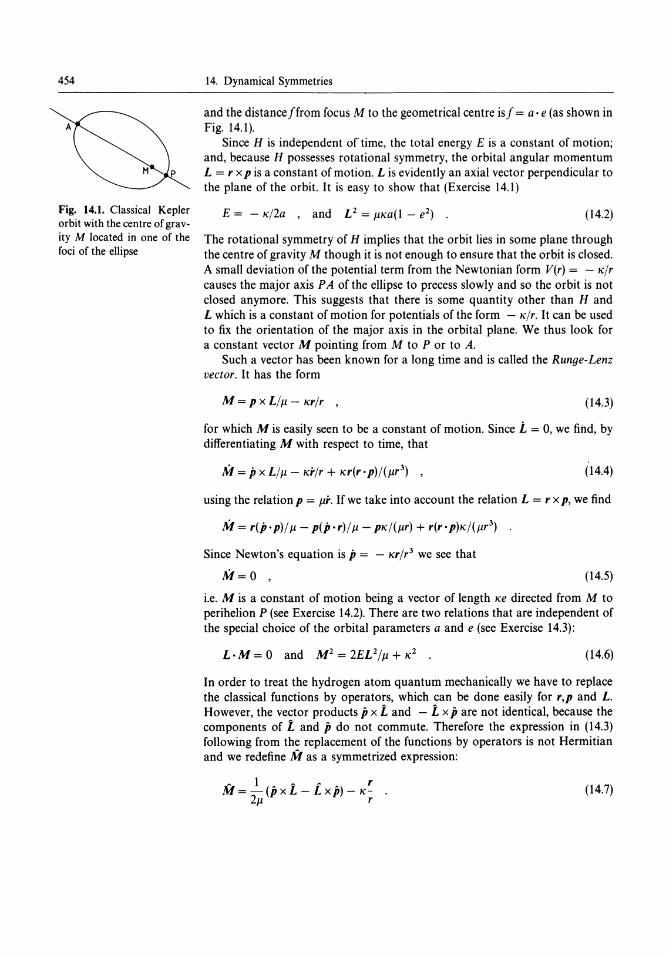
Fig. 14.1. Classical Kepler orbit with the centre of gravity M located in one of the foci of the ellipse


and the distanceJfrom focus M to the geometrical centre isJ = a· e (as shown in Fig. 14.1).

Since H is independent oftime, the total energy E is a constant of motion; and, because H possesses rotational symmetry, the orbital angular momentum L = r x p is a constant of motion. L is evidently an axial vector perpendicular to the plane of the orbit. It is easy to show that (Exercise 14.1)

E = - KI2a , and L2 = JlKa(1 - e2) . (14.2)

The rotational symmetry of H implies that the orbit lies in some plane through the centre of gravity M though it is not enough to ensure that the orbit is closed. A small deviation of the potential term from the Newtonian form V(r) = - Klr causes the major axis P A of the ellipse to precess slowly and so the orbit is not closed anymore. This suggests that there is some quantity other than Hand L which is a constant of motion for potentials of the form - Klr. It can be used to fix the orientation of the major axis in the orbital plane. We thus look for a constant vector M pointing from M to P or to A.

Such a vector has been known for a long time and is called the Runge-Lenz vector. It has the form

M=pxL/Jl-Krlr , (14.3)

for which M is easily seen to be a constant of motion. Since i = 0, we find, by differentiating M with respect to time, that

(14.4)

using the relation p = p';. If we take into account the relation L = r x p, we find

Since Newton's equation is jJ = - Krlr3 we see that

M=O , (14.5)

i.e. M is a constant of motion being a vector of length Ke directed from M to perihelion P (see Exercise 14.2). There are two relations that are independent of the special choice of the orbital parameters a and e (see Exercise 14.3):

L . M = 0 and M2 = 2EL 2 I Jl + K2 . (14.6)

In order to treat the hydrogen atom quantum mechanically we have to replace the classical functions by operators, which can be done easily for r,p and L. However, the vector products p x land - l x p are not identical, because the components of land p do not commute. Therefore the expression in (14.3) following from the replacement of the functions by operators is not Hermitian and we redefine M as a symmetrized expression:

A 1 A A r M = - (p x L - Lx p) - K-

2Jl r (14.7)

14.2 The Group SO(4)

By considering the commutation relations for rand p we can show that

[M,H]_ = 0 ,

L· M = M·L = 0 and

M2 = 2H/p.(L2 + h2) + K2

(14.8)

(14.9)

(14.10)

Relation (14.8) is the quantum-mechanical analogue to (14.5) and the expressions (14.9) and (14.10) correspond to (14.6).

The relations (14.7-10) were used by Pauli in 1926 to calculate the energy levels of the hydrogen atom. He regarded the three components of M as generators of infinitesimal transformations. Following this method we deduce the algebra of the six generators Land M, which consists of 15 commutation relations. Three of these are the known relations for the angular momentum operators:

(14.11)

The commutators that include one component of M and one component of L yield nine further relations,

(14.12)

After some additional calculations, we find the last three commutation relations,

(14.13)

The components of L constitute a closed algebra, as we have seen in Chap. 2, and generate the group 0(3). The i and M together, however, do not form a closed algebra since, although the relations (14.12) involve only M and i, relation (14.13) brings in the operator ii as well. However, given that ii is independent of time and commutes with i and M, we can restrict ourselves to a subspace of the Hilbert space that corresponds to a particular eigenvalue E of Ii. Then ii in (14.13) can be replaced by its eigenvalue E. For bound states E has negative values, and it is convenient to replace M by

M' = J - p./2EM . Evidently (14.12) and (14.13) are thus transformed into

[M;, LJ - = ihejjkM;' and

[M;, Mj] - = ihejjkLk

14.2 The Group SO(4)

(14.14)

(14.15)

(14.16)

The six generators i, M' constitute a closed algebra. To clarify this we relabel the indices of the components of i. First we write

(14.17)

455

456 14. Dynamical Symmetries

for which

[r;, Pj] _ = iMij

holds and we find, because of

iij = riPj - rjPi ,

the "natural indices"

(14.18)

(14.19)

(14.20)

for the i-operators. We now extend the indices to i,j = 1,2,3,4 by introducing fourth components r4 and P4 that fulfil (14.18) and (14.19) and for which

(14.21)

is valid. It is easily verified that (14.18), (14.19) and (14.21) lead to the commutation relations (14.11), (14.15) and (14.16). The six generators iij obviously constitute a generalization of the three generators i from three to four dimensions. The corresponding group can be shown to be the special orthogonal group or the proper rotation group in four dimensions, i.e. SO(4). It includes all real orthonormal 4 x 4 matrices with determinant equal to + 1. This evidently does not represent a geometrical symmetry of the hydrogen atom since the fourth components r 4 and P4 are fictitious and· cannot be identified with geometrical variables. For this reason SO(4) is said to describe a dynamical symmetry of the hydrogen atom. It contains the geometrical symmetry SO(3), generated by the angular momentum operators ii, as a subgroup.

It is essential to note that the SO(4) generators are obtained by restriction to bound states. For continuum states E is positive and the sign inside the square root of (14.14) has to be changed in order for M' to be Hermitian. But then the sign on the rhs of (14.16) changes and the identifications of (14.21) are no longer possible. It turns out that the dynamical symmetry group in this case is isomorphic to the group of Lorentz transformations· in one time- and three space-dimensions, rather than to the group of rotations in four space-dimensions. This is expressed by notation SO(3, 1).

14.3 The Energy Levels of the Hydrogen Atom

It now is comparatively simple to find the energy eigenvalues. We define the quantities

which satisfy the commutation relations

[ii,ij]- =ilieijJk ,

[K;, KJ - = ilieijkKk ,

(14.22)

(14.23)

(14.24)

14.3 The Energy Levels of the Hydrogen Atom

[ii, Kj]_ = 0 ,

[i,H]- = [X, H]_ = 0

(14.25)

(14.26)

Because of (14.25) the algebras of the It and Kk are decoupled; therefore each j and X constitutes a SO(3)- or SU(2)-algebra, and we at once realize the eigenvalues to be

j2 = i(i + 1)1i2 , i = 0, t, 1, ...

X2 = k(k + 1)1i2 , k = 0, t, 1, ...

(14.27)

(14.28)

Relations (14.23)-(14.26) show that the SO(4) group is of rank 2, because one operator 1; and one operator Kj form a maximal system of commutating generators. Thus there are two Casimir operators which may evidently be chosen to be

j2 = i(i + M')2 , and

X2 = i(i - M')2

(14.29)

(14.30)

Alternatively they may be chosen to be the sum and difference of j2 and X2:

C 1 = j2 + X2 = t(i2 + M,2) ,

C2 = j2 - X2 = i. M' .

(14.31)

(14.32)

Equation (14.9) shows that C2 = 0, so that we should only deal with that part of SO(4) for which j2 = X2. Thus i = k, and the possible eigenvalues of C1 are

C1 = 2k(k + 1)1i2 , k = 0,1.1, ...

Transforming (14.31) by taking into account (14.14) and (14.10) yields A 1 A2 A2 2 1 2

C1 = 2(L - EM) = - IlK)4E - 21i ,

so that, using (14.33), the energy eigenvalues are found to be

E = - IlK2/[21i2(2k + 1)2] with k = 0,1.1, ...

(14.33)

(14.34)

(14.35)

Note that one is allowed to use half odd-integer values for i and k; as we soon will see this does not yield any contradiction for the physical quantity i = j + X. Using the triangle rule we see that 1 [in f2 = 1(1 + 1)1i2 ] can have any value in the interval i + k = 2k, ... , Ii - kl = 0 (subsequent values differ by steps of one unit). Obviously 1 is an integer, as it should be in the case of the orbital angular momentum. Also the degeneracy of states is reproduced correctly: i. and K. can each have 2k + 1 independent eigenvalues, and therefore there are altogether (2k + W states. Also, in the preceding chapter we recognized that i is an axial vector, not changing its sign on space inversion. But it is apparent from (14.7) that Mis a polar vector, which does change sign. We thus expect that states characterized by the symmetry generators i and M need not have well-defined parity. This is actually the case, since states of even and odd 1 are degenerate in the hydrogen atom.

457

458

y

x

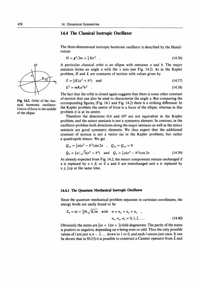
Fig. 14.2. Orbit of the classical harmonic oscillator. Centre of force in the middle of the ellipse


14.4 The Classical Isotropic Oscillator

The three-dimensional isotropic harmonic oscillator is described by the Hamiltonian

(14.36)

A particular classical orbit is an ellipse with semiaxes a and b. The major semi axis forms an angle IX with the x aixs (see Fig. 14.2). As in the Kepler problem, Hand L are constants of motion with values given by

E = !K(a 2 + b2 ) and (14.37)

(14.38)

The fact that the orbit is closed again suggests that there is some other constant of motion that can also be used to characterize the angle IX. But comparing the corresponding figures, (Fig. 14.1 and Fig. 14.2) there is a striking difference: In the Kepler problem the centre of force is a focus of the ellipse, whereas in this problem it is at its centre.

Therefore the directions OA and OP are not equivalent in the Kepler problem, and the minor semiaxis is not a symmetry element. In contrast, in the oscillator problem both directions along the major semiaxis as well as the minor semi axis are good symmetry elements. We thus expect that the additional constant of motion is not a vector (as in the Kepler problem), but rather a quadrupole tensor. We get

QXY = !a(a 2 - b2) sin 2IX , QyZ = Qxz = 0

Qo = taj .j3(a2 + b2 ) and Ql = ta(a 2 - b2 )cos 2IX (14.39)

As already expected from Fig. 14.2, the tensor components remain unchanged if IX is replaced by IX + p, or if a and b are interchanged and IX is replaced by IX ± !7tP at the same time.

14.4.1 The Quantum Mechanical Isotropic Oscillator

Since the quantum mechanical problem separates in cartesian coordinates, the energy levels are easily found to be

E. = (n + !)hJKjm with n = nx + ny + nz ,

nx, ny, nz = 0,1,2, .... (14.40)

Obviously the states are !(n + l)(n + 2)-fold-degenerate. The parity ofthe states is positive or negative, depending on n being even or odd. Thus the only possible values of I are just n, n - 2 .... down to 1 or 0, and each I occurs just once. It can be shown that in SU(3) it is possible to construct a Casimir operator from i and


the quadrupole tensor. Using the spatial representation one can find the relation

C = i 2/h2 + mK/(h2 a2)(Q~y + Q;z + Q;x + Q6 + QD

= - 3 + th2(j;Kr2 + j2/ j;K)2 . (14.41)

If we express the quantities in brackets in terms ofthe Hamiltonian, we find that

C = - 3 + 4m/(3h 2K)H 2 • (14.42)

Substitution of the eigenvalues (14.40) yields

C = t(n2 + 3n) (14.43)

for the nth eigenvalue. Since SU(3) is of rank 2, there are two Casimir operators, which can be characterized by two parameters .l. and {J, and which take on the values 0,1,2, .... The general expression for one of the Casimir operators in terms of these parameters is

(14.44)

Comparison with (14.43) shows that only the representations of SU(3) with (.l., {J) = (n, 0) are realized by the isotropic oscillator. The situation here is somewhat analogous to that in the hydrogen atom, where only the representations of S0(4) with i = k are realized. In contrast to the hydrogen atom we have seen that there is no parity mixing in the isotropic oscillator, since the I values in each degenerate state are either all even or odd. This is to be expected, because all eight generators, i.e. the three components of i and the five components of the quadrupole tensor, do not change sign on space inversion. The group theoretical classification of the isotropic harmonic oscillator plays an important role in the explanation of the structure of light atomic nuclei in the framework of the shell model'.

EXERCISE _____________ _

14.1 Energy and Radial Angular Momentum of the Hydrogen Atom

Problem. Derive relation (14.2).

Solution. In spherical coordinates the Hamiltonian (14.1) is given by

p2 L2 " H=-+--- (1)

2{J 2fJ'2 r

1 e.g. J.M. Eisenberg, W. Greiner: Nuclear Theory, Vol. Ill: Microscopic Theory of the Nucleus, 2nd ed. (North-Holland, Amsterdam 1972).

459

460

Exercise 14.1


At the aphelion ra and the perihelion rp the radial momentum is Pr = 0, so that we have two equations for the total energy:

L2 K E = - - - (Aphelion) . (2a)

2W; ra

L2 K E = --2 - - (Perihelion) .

2Wp rp (2b)

If we divide (2a) by r~ and (2b) by r; and then subtract them from each other, the unknown angular momentum is eliminated, yielding

E(r. + rp) = - K • (3)

By subtracting (2) directly we have, in addition, that

L2 2J.t (ra + rp) = Kr.rp . (4)

With the help of the geometrical relations ra = a + J, rp = a - f and f = (a 2 - b2)1/2, we find that

rp + r. = 2a and rarp = a2 - f2 = b2 •

Equations (3) and (4) thus yield the desired result.

K E= -2a .

L2 = 2J.tKr.rp /(r. + rp) = J.tKb 2/a = J.tKa(l - e2)

EXERCISE

14.2 The Runge-Lenz Vector

Problem. Show that the Runge-Lenz vector can be written in the form

M = Kerp/rp ,

(5)

(6)

(7)

(1)

where rp is the vector directed from the centre of the ellipsoidal orbit to the perihelion, and e is the eccentricity.

Solution. We start with (14.3). Since M is a constant of motion, we can evaluate the rhs for r = rp and, because of the relation L = r x p, r, p and L form a righthanded system of vectors at every point of the orbit. At the perihelion rand pare perpendicular, that is, p x L is oriented in the same way as r. This can easily be seen using the general rule for double cross products:

p x L = p x (r x p) = rp2 - p(r· p) , (2)


yielding

(p x L)p = rpp2 = rpL 2 jr~ (3)

at the perihelion. With the help of (3) we have, using rp = a - f = a(l - e),

1 Ka(l - e2 ) -(, x L)p = rp (1 ) = rpK(l + e)jrp (4) J.! a - e rp

This enables us to write the desired equation for !VI, i.e.

(5)

EXERCISE _____________ _

14.3 Properties of the Runge-Lenz Vector Nt

Problem. Derive relation (14.6).

Solution. First we prove (6a) by writing

1 K L·M = -L·(px L) - - L xr

J.! r

K = - - (r x p) x r = 0 ,

r (1)

because a mixed product including two identical vectors always vanishes. Next we establish (6b) through

1 K M2 = _(pXL)2 - 2-(px L).r + K2

J.!2 /lr

1 2 2 2 K 2 =-[p L -(p·L) ]-2-(rxp)·L+K J.!2 /lr

1 K = - (p2 L 2) _ 2 _ L 2 + K2 ,

J.!2 J.!r (2)

because again p. L = p. (r x p) = O. The first two terms can be combined to produce

(3)

461

Exercise 14.2

462 14. Dynamical Symmetries

EXERCISE _____________ _

14.4 The Commutator Between M and Ii

Problem. Prove the quantum mechanical relation

- fl2 C [M, Ii] _ = 0 for H = - - - and 2m r

- 1 - - P M = - (fl x L - Lx fl) - c-2p. r

Solution. Since we only have to deal with operators in the rest of the exercises in this chapter, confusion is hardly possible so from now on for convenience we drop the operator sign. It is well known that the above Hamiltonian commutes with the angular momentum operators, [H, L;] _ = 0, for all i. Next we calculate two auxiliary commutators, necessary for the subsequent calculations:

Now we have

and therefore

[ Xi '" 2J 2 ( Xi 1 !l Xi '" !l) i' f Pk _ = 21i - r3 + ;Ui - r3 f XkUk

For the commutator in question we have

[Mh H] - = 2~ [(p x L - Lx p);, H] - - c [~, H 1 ' and the second commutator can be further reduced yielding

C [Xi'" 2J - - -,,-,Pk , 2m r k _

(1)

(2)

(3)


which just corresponds to (2). The first commutator is then treated in the following way:

[(, x L - L xp);, HJ- = Leijk[(PjLk - LjPk), HJjk

(4)

Since Hand L commute, H can be brought into the left-most position [note (1)] so that

Now we insert L j = L.m,nejmnXmPn and the analogous expression for Lk and find

[(, x L - L xp);, HJ- = ilic L eijk jkmn

(5)

To proceed further we use the simply derived auxiliary commutator

and thus we have

[(p x L - L xp);, HJ-

'Ii 2 '" {XmXk X jXm} = -(I ) C L... eijk ejmn -3- - ekmn -3- On jkmn r r

(6)

L.m,neijmnXmXn vanishes for all j, as can easily be seen by explicit notation, since [xm' xnJ - = 0 in the last term of (6). The indices j and k may be interchanged in the second term of the first sum, yielding (by use of eikj = - eijk) the first term of this sum once again. Now we have

using the relation

(7)

463

Exercise 14.4

464

Exercise 14.4


which can easily be verified. The second sum in (6) can be simplified with the help of this relation, too, i.e.

Collecting all the contributing terms, we find on the one hand, using (6), that

1 • c . 2 (Xi 1 Xi I ) -[(pxL-Lxp)i,H]_ =-(IIi) ---Oi+- XkOk (8) 2m m r3 r r3 k

and on the other hand from (2) that

-c -, H = - - (Iii) - - - Oi + - XkOk [ Xi ] C . 2 (Xi 1 Xi I ) r _ m ,3, ,3 k

(9)

Adding Eqs. (8) and (9) yields [Mi' H] _ = 0.

EXERCISE ______________ _

14.5 The Scalar Product i· Nt

Problem. Prove the quantum mechanical relation i· Nt = 0, using the definition of Nt given in Exercise 14.4.

Solution. a) We have L· r/r = ° since

(1)

Since Li.meimnXmXi == 0, the first sum vanishes, as does the second because of eimm == 0.

b) Furthermore we have L· (p x L) - L ·(L x p) = ° due to

I eijk Li(pjLk - LjPk) = I Li I eijk(ekmnPjmmPn - ejmnXmPnPk) ijk i jkmn

jm" kmn

(2)

(in the last transformation we have changed the summation index from k to j). Using the commutation relations for x and p, [Pj' Xi] _ = - ilibij' we end up


with

t Li { ~ (PjXiPj - PjXjPj - XjPiPj + XiPj) }

L eimnXm(pn PjXi Pj - PnPj XjPi ijmn ~ ~

- pn XjPi Pj + ~

xiPj-iMij Pixj+iMij PiXj + iMij

- ~ XjPj - iliPn(;ijPj + ~ PnpJ - iii ~ pJ )

= 0 after sum = 0 after sum = 0 since over n,i over m, i £imi=O

over i.m £imi=O

~ PiPjXj - iMijPnPj - iIiPn(;ijPj)

=0 after sum over n, i

L eimnXm( - 3iMijPnPj) = 0 ijmll

since

imn m in

(3)

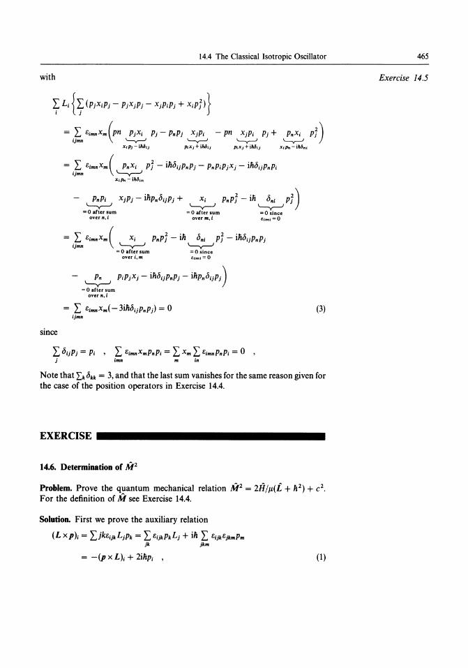
Note that Lk (;kk = 3, and that the last sum vanishes for the same reason given for the case of the position operators in Exercise 14.4.

EXERCISE _____________ _

14.6. Determination of M2

Problem. Prove the quantum mechanical relation M2 = 2H/f.l(i + 1i 2 ) + c2.

For the definition of M see Exercise 14.4.

Solution. First we prove the auxiliary relation

(L XP)i = LjkeijkLjPk = L llijkPk Lj + iii L eijkejkmPm jk jkm

(1)

465

Exercise 14.5

466

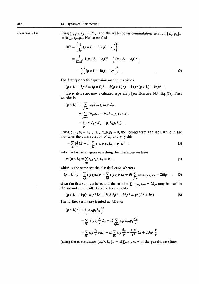
Exercise 14.6


using Lj.kejkiejkm = 2bim and the well-known commutation relation [Lj, Pk]= iii LmejkmPm' Hence we find

M2 = - (p x L - L x p) - c -{ I r}2 2/1 r

= _1_ 4(p x L - ilip)2 - ::.. (p x L - ilip) " ~ (2/1)2 /1 r

cr. 2 r2 - - - (p x L - llip) + c -

/1 r r2 (2)

The first quadratic expression on the rhs yields

(p x L - ilip)2 = (p X L)2 - ili(P x L)"p - ilip-(p x L) _li 2p2

These items are now evaluated separately [see Exercise 14.4, Eq. (7)]. First we obtain

ijkmn

jkmn

= L (Pj LkPj Lk - pjLkPkLJ . jk

Using L.kLkPk = L.k.m .• ekm.XmP.Pk = 0, the second term vanishes, while in the first term the commutation of Lk and Pj yields

= L pJ Lf + iii L ekjmPjPmLk = p2 L 2 , (3) jk jkm

with the last sum again vanishing. Furthermore we have

(4) ijk

which is the same for the classical case, whereas

(p x L)" p = L EijkPjLkPi = L ejjkPjPiLk + iii L eijkekimPjPm = 2ilip2 , (5) ijk ijk ijkm

since the first sum vanishes and the relation L.k,iEkijEkim = 2bjm may be used in the second sum. Collecting the terms yields

(px L - ilip)2 = p2L2 - 2(ili)2p2 _li2p2 = p2(L2 + li 2) (6)

The further terms are treated as follows:

(using the commutator [x;!r, Lk] _ = iii L.m Eikm xm/r in the penultimate line).


The second sum, however, vanishes since. Iliik == 0 and L.i,j,kllijkXiXj == O. Substitution of L.i,JllijkXiPj by Lk yields

(7)

Altogether we find that

~(pxL - ilip) + (pxL - ilip)·~ = !L2 - ili~·p + !L2 r r r r r

2i1i r 'Ii r + P--l po- , r r

and, using po r/r = r/r· p - 2ililr, we get

2 2 2 2 2 1i2 ) =-L --. -=-(L + . r r(IIi)2 r (8)

Collecting all these partial results we end up with

1 c2 M2 = __ 4p2(L2 + 1i2) ___ (L2 + 1i2) + c2 , (2#l)2 #l r

and therefore

M2=~(p2 _~)(L2+1i2)+C2 ,M2=~H(L2+1i2)+c2 (9) #l 2#l r Il

EXEROSE .......................... .

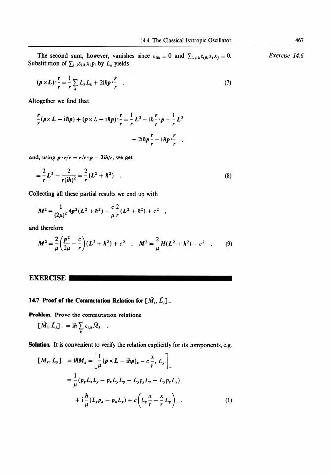
14.7 Proof of the Commutation Relation for [M;, I j ]_

Problem. Prove the commutation relations

[M;, i j ]_ = iii L lliJkMk • k

Solution. It is convenient to verify the relation explicitly for its components, e.g.

[M", L,]_ = iliM% = [! (p x L - ilipl. - c:', L1] #l r_

(1)

467

Exercise 14.6

468

Exercise 14.7


We have

and

and therefore

In addition,

Lyp" - p"Ly = -ihpz , and Ly': - .: Ly = -ih:' , r r r

using the commutation relation [L;, Pk] - = ih Lm6ikmPm already mentioned in Exercise 14.6; thus we obtain

[M", L,]_ = i ~ (p"Ly - p,L" - ihp.) - ihc:' = ihM. . ~ r

(2)

What we still have to prove is that, e.g., [M", L,,] = O. Continuing, we write

which leads to

pyL.L" = p,L"L. + ihp,L, = L"p,L. - ihp.L. + ihpyLy , and

p.LyL" = p.L"Ly - ihp.L. = L"p.Ly + ihpyLy - ihp.L. ,

yielding

(3)

(4)

Furthermore L"p" - p"L" = 0, but also L"xlr - xlrL" == 0 (since [xi/r, Lj]_ = ihLk6ijkxklr). So we end up with

(5)

The remaining commutation relations can be derived by cyclic permutation of x, y, and z.


EXERCISE _____________ _

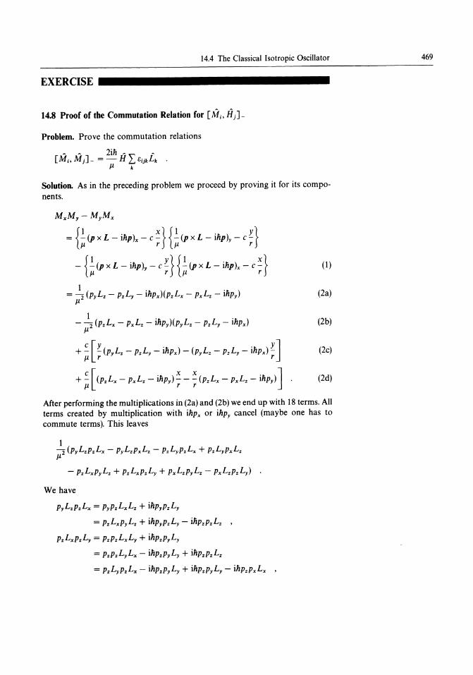
14.8 Proof of the Commutation Relation for [Mi , H)]_

Problem. Prove the commutation relations

Solution. As in the preceding problem we proceed by proving it for its components.

{ I . X}{l . Y} = - (p x L - llip)x - c - - (p x L - I lip ) - c -J1 r J1 y r

- {~(Px L - ilip) - c~} {~(px L - ilip)x - c~} (1) J1 y r J1 r

= -.; (pyLz - pzLy - ilipx)(pzLx - PxLz - ilipy) (2a) J1

- -.; (pzLx - PxLz - ilipy)(pyLz - pzLy - ilipx) (2b) J1

+ :. [~(PYLz - pzLy - ilipx) - (pyLz -- pz Ly - ilipx) ~J (2c) J1 r r

+ :. [(PzLx - PxLz - ilipy) ~ - ~ (pzLx - PxLz - iliPY)] (2d) J1 r r

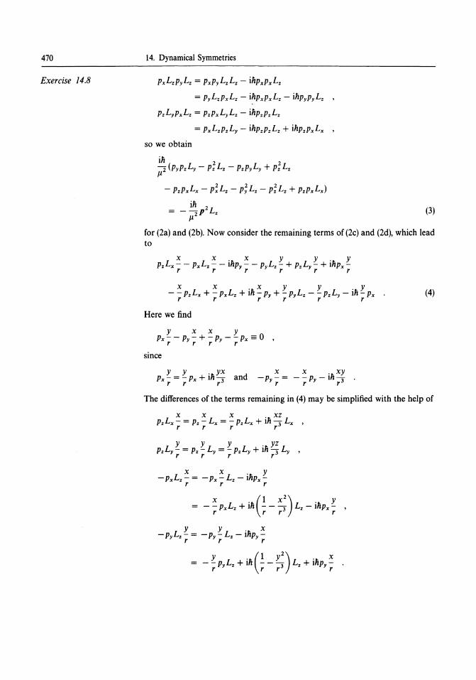
After performing the multiplications in (2a) and (2b) we end up with 18 terms. All terms created by multiplication with ilipx or ilipy cancel (maybe one has to commute terms). This leaves

We have

pyLzpzLx = pypzLxLz + ilipypzLy

= pzLxpyLz + ilipypzLy - ilipzpzLz ,

pzLxpzLy = pzpzLxLy + ilipzpyLy

= pzpzLyLx - ilipzpyLy + ilipzpzLz

= pzLypzLx - ilipzpyLy + ilipzpyLy - ilipzPxLx ,

469

470

Exercise 14,8

14, Dynamical Symmetries

PxLzpyLz = PxpyLzLz - ilipxPxLz

= pyLzPxLz - ilipxPxLz - ilipypyLz ,

pzLyPxLz = pzPxLyLz - ilipzpzLz

= PxLzpzLy - ilipzpzLz + ilipzPxLx ,

so we obtain

- pzPxLx - p;Lz - p; Lz - p; Lz + pzPxLx)

iii 2 -2'P L z

J.1 (3)

for (2a) and (2b), Now consider the remaining terms of (2c) and (2d), which lead to

x x, x y y, Y pzLx - - PxLz - - llipy - - pyLz - + pzLy - + llipx-

r r r r r r

x x ,x y y ,y - - pzLx + - PxLz + Iii - py + - pyLz - - pzLy - Iii - Px

r r r r r r (4)

Here we find

y x x y Px - - P - + - p - - Px == 0 r Yr r y r

since

The differences of the terms remaining in (4) may be simplified with the help of

x x x ,xz pzLx - = pz - Lx = - pzLx + 11i:3 Lx ,

r r r r

y y y , yz pzLy - = pz - Ly = - pzLy + Iii "3 Ly ,

r r r r

x x 'Ii y - PxLz - = - Px - Lz - I Px-r r r

x 'Ii(l X2) 'Ii Y = - - PxLz + I - -:3 Lz - I Px - , r r r r

L Y Y 'Ii x -p -=-p-L-Ip-YZr Yr Z Yr

Y 'Ii(l y2) 'Ii x = - - P Lz + I - - - Lz + I P -r Y r r3 Y r


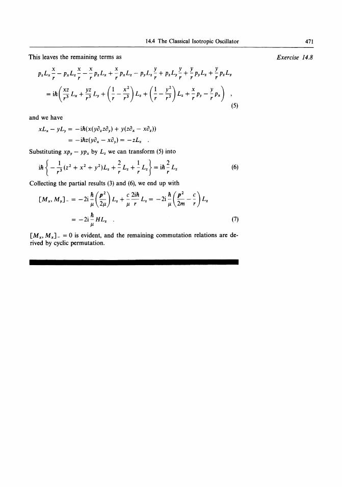
This leaves the remaining terms as

. (xz yz (1 X2) (1 y2) x y) = Iii - L" + - L + - - - Lz + - - - Lz + - P - - p" , r3 r3 y r r3 r r3 r Y r

and we have

xL" - yLy = -ili(x(yozZOy) + y(zo" - xOz))

= -iliz(yo" - XOy) = -zLz .

Substituting Xpy - yp" by Lz we can transform (5) into

(5)

iii {- 13 (Z2 + x2 + y2)Lz + ~ Lz + ! Lz} = iii ~ Lz (6) r r r r

Collecting the partial results (3) and (6), we end up with

[M", M ]_ == -2i ~ (p2) Lz +.: 2ili Lz = -2i ~ (p2 -~) Lz y p. 2p. p. r p. 2m r

= -2i ~ HLz (7) p.

[M", M,,]_ = 0 is evident, and the remaining commutation relations are derived by cyclic permutation.

471

Exercise 14.8

Documents

Quantum Mechanics || Dynamical Symmetries