Embed Size (px)
Citation preview
Foundations of Physics. Vol. 25, No. 2, 1995
Quantum Mechanical States as Attractors for Nelson Processes ~
Nicola Cufaro Petroni 2 and Francesco Guerra 3
Received May 13. 1994
hi this paper we reconsider, in the light of the Nelson stochastic" mechanics, the idea orightally proposed by Bohm and Vigier that arbitrary sohttions of the evohl- tion equation for the probability densities ahvays relax ht time toward the quantmn mechanical density Iq/l'- derived fi'om the Schrddinger equation. The analysis o f a few general propositions attd o f some physical examples show that the choice of the L i metrics and of the Nelson stochastic f lux is correct for a particular class o[' quantum states, but cannot be adopted ht general. This b~dicates that the question i f the quantum mechanical densities attract other sohttion of the classical Fokker-Planck equations associated to the SchrCdhtger equation is physically mean#~gful, even i f a classical probabilistic model good for ever T quantum state is still not available. A few suggestion ht this dh'ection are finally discussed.
1. I N T R O D U C T I O N
In an important old paper ~ Bohm and Vigier have discussed the possi- bility that some criticisms to the assumptions of the causal interpretation of the quantum mechanics ~2~ could be overcome by means of an extension of the hydrodynamical model initially proposed by Madelung ~3~ in the direction of allowing that the Madelung fluid "undergoes more or less random fluctuations in its motion." In particular this model, given in terms of a fluid with irregular fluctuations, was supposed to answer a criticism of Pauli and others ~4~ about the hypothesis, made in the causal interpretation, that, if ~,(r, t) satisfies the nonrelativistic Schr6dinger equation, then the
Written in honor of J.-P. Vigier. -" Dipart imento di Fisica dell' Universitfi and I.N.F.N., via Amendola 173, 70126 Bari, Italy. 3 Dipar l imento di Fisica dell' Universitfi La Sapienza and I.N.F.N., piazzale A. Moro 2, 00185
Roma, Italy.
297
[1015-9()1~ 95~0200-0297507.500 ,c 1995 Plenum Publishing Corporation
298 Petroni and Guerra
probability density function (pdf) in an ensemble of particles with this wave function is f(r , t ) = ]~(r, t)] 2. The physical idea of Bohm and Vigier was that, even if our ensemble of quantum systems is described by an arbitrary initial pdf it will decay in time to an ensemble with pdf I~p] 2, because of the random fluctuations arising from the interactions with a subquantum medium: "no matter what the initial probability distribution may have been (for example, a delta function) it will eventually be given by P = ]~b[2. ' ' In the work cited above, however, some mathematical difficulties made the general proof of this property less than complete.
On the other hand this paper can historically be considered as a stepping stone on the way to the understanding of the deep relations connecting the quantum mechanics with the world of the classical random phenomena. Researches in this field eventually led to the formulation of the stochastic mechanics~5): a classical model where the particles follow continuous random trajectories in space-time and all the observable predic- tions of the quantum mechanics can be completely reproduced. This theory is "by no means a causal theory, but probabilistic concepts enter in a classical way. ''~5~
The aim of the present paper is to review, in the light of the stochastic mechanics, the old idea of Bohm and Vigier about the decay of every initial pdf toward the quantum mechanical pdf: in Sec. 2 we will briefly recall the fundamentals of the Bohm and Vigier model and the principles of the stochastic mechanics; in Sec. 3 we will discuss a few general properties of the time evolution of the pdf's of the Markov processes in the particular metric induced by the usual norm in L~(R); in Sec. 4 we discuss a few specific examples of quantum systems described in stochastic mechanics and we show that, in the chosen metrics, the trend of all the initial pdf's to decay in time toward the quantum mechanical pdf is not a general property since it holds only for a wide but particular class of wave func- tions; finally in Sec. 5 a short discussion follows about these results and the possibility of their generalization.
2. THE CAUSAL INTERPRETATION AND THE STOCHASTIC MECHANICS
The causal interpretation of the quantum mechanics is based on the idea that a nonrelativistic particle of mass m, whose wave function obeys the Schr6dinger equation
h 2 .~
il)O,t~(r, t )= -2--mn V-~(r, t ) + V(r, t) ~(r, t) (1)

Quantum Mechanical States as Attractors 299
is a classical object following a continuous and causally defined trajectory with a well-defined position and accompanied by a physically real wave field ~ which contributes to determine its motion. In fact, if we write down ( 1 ) in terms of the real functions R(r, t) and S(r, t) with
~,(r, t) = R(r, t) e iS(,'t)/h (2)
and separate real and imaginary parts, we have
O'R2 + V ( Rz VS~=O,n / (3)
_--=----(VS)2 V h2 V2R 0 (4) 0 ' S + 2m + 2m R
where R2(r, t) = I~b(r, 012 is interpreted as the density of a fluid with stream velocity
VS v(r, t ) = - - (5)
m
Thus Eq. (3) expresses the conservation of the fluid while Eq. (4) plays the role of a Hamil ton-Jacobi equation for the velocity potential S in the presence of a quantum potential
h 2 V2R
2m R
which depends on the form of the wave function. In the causal interpreta- tion the particle follows deterministic trajectories dictated by (5) when v is identified with the velocity of a particle passing through r at the time t.
It is important to remark now that, if we define
VS h VR-" v(+~(r, t ) = - - m + 2,n R 2 (6)
the continuity equation (3) takes the form
OtR- =2-ram V R- - - v ( a - ' v ( + l ) (7)
so that R 2 can also be considered as a particular solution of the evolution equation of the pdf's of a Markov process (Fokker-Planck equation)
a,f= v V 2 f - V(b, +,) (8)
825 25 2-8

300 Petroni and Guerra
characterized by the velocity field v~ +~ and by a diffusion coefficient
h v = - - (9)
2m
This points out a possible connection between the density R 2 of the Madelung fluid and the pdf of a suitable Markov process describing the random motion of a classical particle. As a matter of fact this connection is not at all compulsory at this point since the causal interpretation is a deterministic theory with no randomness involved in its fundamentals so that the analogy between (7) and (8) could also be considered purely formal. Moreover it must be remarked that, while for a given v~+) we can determine an infinity of solutions of (8) (one for every initial condition f ( r , 0 ) = f 0 ( r ) ) which are pdf's of Markov processes, the quantum mechanics are characterized by the selection of just one particular solution f = R 2 among all the possibilities. In fact it must be emphasized that R 2 and v~+~ are not independent: they are both derived from a ~b solution of (1) and hence are locked together by their common origin. In other words: not every couple off , solution of (8), and v~ + I can be considered as derived from the same solution of the Schr6dinger equation through the relation (6) and f = R'-.
That notwithstanding, the causal interpretation is obliged to add some randomness to its-deterministic description in order to reproduce the statistical predictions of the quantum mechanics and hence it identifies the function R 2 = [~'l-" with the pdf of an ensemble of particles. But, since this addition is made by hand, is it easy for the critics of the model to argue that "it should be possible to have an arbitrary probability distribution (a special case of which is the function P = 6 ( x - Xo) representing a particle in a well-defined location) that is at least in principle independent of the ~, field and dependent only on our degree of information concerning the location of the particle. ''~1
A more convincing connection between quantum mechanics and classi- cal random phenomena was achieved only later by means of the stochastic mechanics~6~: here the particle position is promoted to a stochastic Markov process ~(t) defined on some probabilistic space ( s P) and taking values (for our limited purposes) in R 3. This process is characterized by a pd f f ( r , t) and a transition pdf p(r, t i t ' , t ') and satisfies an It6 stochastic differential equation of the form
d~(t) = v~ + ~(~(t), t) dt + dJt(t) (10)
where v(+~is a velocity field which plays the role of a dynamical vari- able not given a priori but subsequently determined on the basis of a
Quantum Mechanical States as At t rac to r s 301
variational principle, and t/(t) is a Brownian process independent of ~ and such that
E(dr/(t)) = 0, E(dr/(t) drt(t)) = 2vI dt
where dq(t)=~l(t+dt)-q(t) (for dt > 0), v is the diffusion coefficient, and I is the 3 • 3 identity matrix. We know that under fair analytical conditions on the velocity field v~§ the solution of (10) exists and is unique if we supplement our equation with the initial condition 8(0) = ~o; moreover, the pdf of the process satisfies the evolution equation (8) associated with the initial condition f ( r , 0 ) = f o ( r ) iffo(r) is the pdf of 8.0. An important role is played by the family of the transition pdf's p(r, t iP , s) which are defined as the conditional pdf's of our process under the hypothesis that ~ ( s )= r': in particular p(r, t [ r ' , 0) will be the solutions of (8) if we choose as initial condition Co = r ' (P-a.s.). The relevance of the transition pdf is well appre- ciated when we realize that every other solution of (8) (which satisfies the boundary and the non-negativity conditions to be a pdf) is propagated from its initial condition fo(r) following the prescription
f(r,t)=fa3p(r, tlr',O)fo(r')d3r', t > O (11)
or more generally
f (r , t )=f~ p(r, tlr',s)f(r',s)d3r ', t>s (12)
In other words the transition pdf's, also calledfimdamental sohaions of (8), play the role of the propagators and are the solutions of (8) which satisfy (in the sense of the distributions) the initial conditions
p(r, t I r', O) ~ 8 ( r - r'), t -*O + (13)
A suitable definition of the Lagrangian and of the stochastic action functional for the sytem described by means of the dynamical variables f and v~ + ~ allows us to select, by means of the principle of stationarity of the action, the particular processes which reproduce the quantum mechanics. More precisely the selected processes will have a drift velocity
vf

302 Petroni and Guerra
which, as required in (5), is always the gradient of a particular function
S(r, t) solution of (4) with R = x/"-f. Moreover, it is possible to show that from f and S selected in this way we can always build a wave function
~,(r, t) = ~/f(r , t) e is''''vh
which satisfies the Schr6dinger equation (1). In this formulation the foundations to interpret R 2 as a particular
solution of a Fokker-Planck equation for the pdf of Markov processes are well established. Of course we pay for this by abandoning the idea of deter- ministic trajectories even if the stochastic mechanics keeps intact the description by means of continuous trajectories in space-time and recovers the paths of the causal interpretation as averages on the stochastic trajectories. In this perspective the idea proposed by Bohm and Vigier of a relaxation in time of arbitrary pdf's solutions of (8) toward the quantum mechanical pdf 4qJl 2 can be checked as a property of the solutions of the Fokker-Planck equations with the field v~+l derived according to (6) from the wave functions solutions of (1). In other words, in this paper we will analyze an updated version of the Bohm and Vigier idea that for every quantum wave function ~ there exists a stochastic flux, described by a family of transition pdf's p(r, t l r ' , s ) , such that: (a) the quantum pdf [~[2 is correctly propagated by p; (b)every other pdf propagated by p approximates, in a suitable sense, the quantum pdf [~[2 for t ~ +oz. In particular, we will explore the possibility that the p associated by the Nelson stochastic mechanics to a quantum state ~b can be interpreted as the origin of the Bohm and Vigier stochastic flux, namely we will examinate if and how the solutions of (8) selected by the stochastic mechanics to reproduce the quantum predictions attract other solutions which do not satisfy the stationary stochastic action principle and hence cannot be considered as describing quantum systems.
3. TIME EVOLUTION OF THE MARKOV PROCESSES
In what follows we will limit ourselves to the case of the one-dimen- sional trajectories, so that the Markov processes ((t) considered will always take values in R. The set of all the probability density functions of the absolutely continuous real random variables defined on a probability space (s ,7, P) coincides with the set ~ of all the non-negative functions f ( x ) of the hypersphere of norm 1 in the Banach space L~(R) with norm
f + .:t..
IIfll : I A x ) l dx

Quantum Mechanical States as Attractors 303
and hence the time-dependent pdff (x , t) of the stochastic processes ~(t) will be considered as trajectories on this subset ~. For Markov processes the transition pdf's p(x, t l y, s) classified by means of the initial condition ~(s)= y (with s < t) are particular trajectories with nonabsolutely con- tinuous initial conditions. In .~ we can then introduce a metric induced by the norm in L~(R):
d(f, g) = �89 If(x) - g(x)l dx
Here the factor 1/2 guarantees that we always have 0~<d(f, g)~< I: the value 1 is attained when f and g have disjoint supports, and the value 0 when they coincide (Lebesgue almost everywhere).
Definition 1. We will say that the pdff(x, t) Lt-approximates the pdf g(x, t) (for t ~ +o~), and we will write
f ( x , t) LI g(x, t), t ~ + ~
when
d(f, g) ---, 0, t --* + ~
In particular we will say that f L l-converges toward g (for t ~ +or) if the pdf g(x) does not depend on the time t.
This means that the two trajectories on the unit hypersphere tend to approximate one another in the Ll-norm when t ~ + ~ . If the stochastic processes ~(t) under examination are Markov processes (as happens in stochastic mechanics) satisfying the stochastic differential equation (10) with initial condition ~(0)= ~0, their pdf will satisfy the one-dimensional evolution equation
a, f (x , t )= rOOf(x, t)-O,.(v~+)(x, t) f ( x , t)) (14)
with the initial condition f ( x , O) =fo(x) iffo(x) is the pdf of Go. We will examinate next a few properties of the concept of L~-approxi -
mation for processes satisfying Eq. (10).
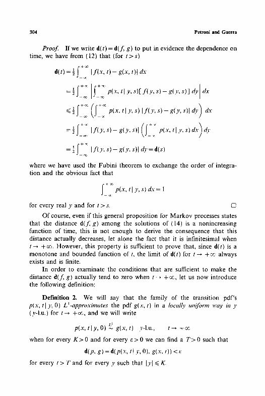
Proposition 1. If f and g are solutions of (14), the distance d ( f g) is a monotonic nonincreasing function of the time t.
304 Petroni and Guerra
Proof If we write d ( t ) = d ( f , g) to put in evidence the dependence on time, we have from (12) that (for t > s)
f -t- ,zc, d(t) = �89 If(x, t ) - g(x, t)l dx ~z
=~_ -~.. p(x, t ly , s ) [ f ( y , s ) - g ( y , s ) ] d y dx
<~�89 p(x, t ly , s ) I f ( y , s ) - g ( y , s ) l dy dx
= �89 tly, s) dx )dy
=�89 [ f ( y , s ) - g ( y , s ) l dy = d(s)
where we have used the Fubini theorem to exchange the order of integra- tion and the obvious fact that
for every real y and for t > s.
p(x, t[ y, s) dx = 1
[]
Of course, even if this general proposi t ion for Markov processes states that the distance d(f , g) among the solutions of (14) is a nonincreasing function of time, this is not enough to derive the consequence that this distance actually decreases, let alone the fact that it is infinitesimal when t ~ +c~. However, this proper ty is sufficient to prove that, since d(t) is a monotone and bounded function of t, the limit of d(t) for t---, + ~ always exists and is finite.
In order to examinate the condit ions that are sufficient to make the distance d ( f g) actually tend to zero when t---, +c~, let us now introduce the following definition:
Definition 2. We will say that the family of the transit ion pdf 's p(x, t[ y, O) LI-approximates the pdf g(x, t) in a locally w~iform way in ), (y-l.u.) for t + + m , and we will write
p(x, tl y, O) ~ g(x, t) y-l.u., t ~ + ~
when for every K > 0 and for every e > 0 we can find a T > 0 such that
d(p, g ) = d(p(x, tl y, 0), g(.x, t ) ) < e
for every t > T a n d for every y such that lYl ~<g.

Quantum Mechanical States as Attractors 305
The meaning of this definition is the following: the transition pdf's which L'-approximate the same pdf g for t-~ +or progressively forget their dependence on the initial condition y, in the sense that, for every y, they approximate the same pdf g. Moreover, the local uniformity in y requires something more than the simple L~-approximation of every p to the same g independently from y, albeit something less than the global uniformity which would ask that the inequality d(p, g ) < e be verified for every t > T and for every real y without limitations. Of course the global uniformity implies the local uniformity, but the converse is not in general true.
Proposition 2. If the transition pdf's p(x, t]y, 0) L l-approximate y-l.u, the pdf g(x, t) for t-~ + ~ , then every f(x, t) solution of the evolu- tion equation (14) Ll-approximates g(x, t) for t-~ + ~ .
Proof Let f(x, t) be an arbitrary solution of (14), corresponding to the initial condition f (x , 0 )=fo(x) , and e > 0 an arbitrary positive number. Since fo is in LJ(R) we will always be able to find a K > 0 such that
f~,.~ > K fo(y) dy <2
Moreover, since the approximation is y-I.u., for the given e and K we can always find T > 0 such that
I f +'~' d(p, g ) = ~ -~, ]p(x, tl y, O)- g(x, t)l dx < 2
for every t > T and for every real y such that lyl ~< K. Then, since we always have d(p, g) ~< 1, we get for every t > T
1 f4-~, d(f, g)= 5 3_~
l f+ ~'
1 r 2 ~,
- , (lf+
]f(x, t )-- g(x, t)l dx
[p(x, t[ y, O) - g(x, t)] fo(Y) dy dx
Ip(x, t y , O ) - g ( x , t) l fo(y)dy)dx
]p(x, tl y, O)-- g(x, t)l dx) dy
f +~ = fo(Y) d(p, g) dy

306 Petroni and Guerra
=f fo(y) d(p,g)dy+] f0(y) d(p, g) dy l y l > X I: '1 ~ K
K d e .<K e e e <fl,,l> fo(Y) Y+2fl,'l f~ dY<-2+2=
where we used all the previous limitations and the Fubini theorem to exchange the order of integration. []
Let us remark that in the proof we nowhere used the hypothesis that g(x, t) is a solution of (14): in fact, it is enough to suppose that g is the time-dependent pdf of a generic Markov process. However, even if the transition pdf's p L~-approximate a g which is not a solution of (14) the triangular inequality for the metric d allows us to show that all the solutions of (14) LLapproximate one another as stated in the following proposition:
Corollary 1. If the transition pdf 's L~-approximate y-l.u, an arbitrary pdf g, then
d(f l , f2) ~ 0, t--* + ~
for every f l , f2 solutions of (14).
Proof From Proposit ion 2 we have fl L' L t g and f2 ~ g so that from the triangular inequality
d(f~,f2)<~d(fi, g)+d(f2, g)~O, t~ +c~ for every f l and f2 solutions of (14). []
The meaning of this Corollary is that, under the conditions of Proposition 2, all the solutions of (14) globally tend to L~-approximate one another after a sufficiently long time. Vice-versa, if we can find two solu- tions f l and f2 of (14) such that d ( f l , f 2 ) is not infinitesimal for t ~ +or , then no pdf g can be L~-approximated y-l.u, by the family of the transition pdf's p.
4. EXAMPLES FROM QUANTUM MECHANICS
In order to discuss our examples in detail it will be useful to derive a formula to calculate the L~-distance among the pdf's ~U(m, t&) of normal random variables, namely pdf 's of the form
e - ~ x - m )2/2o 2
g .... (x) = ~ v / ~

Quantum Mechanical States as Attractors 307
with real m and a > O. In the following we will indicate with the symbol
1 f" ~ ( x ) = ~ _ ~ e -.,.-'/2 dy
the usual error fimction and we will also pose
d(a, b; p, q)=d(ga. ~, gt,.q)
Proposition 3. With the previous notations, i f p > q we have that
d ( a , b ; p , q ' = I ~ ( ~ 2 ~ ) - ~ ( ~ ) l
where
aq2 _ bp2 _ qp x/(a _ b)2 + 2(q2 _ pZ) In(q/p) Xl = q 2 p 2
aq'- -- bp 2 + qp x/( a - b) 2 + 2(q 2 - p2) In(q/p) x2 = q2 _ p2
If p = q and a 4: b we have that
d ( a , b ; p , p , = 2 ~ ( ~ ) - I
Finally, i f p = q and a=b we have that d(a, a; p, p ) = 0 .
Proof The points where the difference between the two normal pdf 's change its sign are the solutions of the equation
(q2-p2) x 2 - 2 ( a q 2 - b p 2 ) x + [a2q2-b2p2 + 2q2p21n(p/q)]=O (15)
If p=/:q (in particular, to fix the ideas, if p>q) the solutions are the numbers x~ and x2 indicated in our proposi t ion which are always real since
(q2-- p2) ln q= P2 [ ( q ) 2--111n P
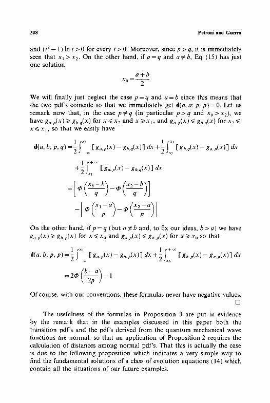
308 Petroni and Guerra
and (1'2 _ 1 ) In t > 0 for every t > 0. Moreover, since p > q, it is immediately seen that x~ > x 2. On the other hand, i f p = q and a # b , Eq. (15) has just one solution
a + b NO ~ 2
We will finally just neglect the case p = q and a = b since this means that the two pdf's coincide so that we immediately get d(a, a; p, p ) = 0 . Let us remark now that, in the case p # q (in particular p > q and x~ >x2), we have gu. p(x) >~ gh, q(X) for x ~< x2 and x >/Xl, and go.p(x) <~ gl,.q(x) for x2 ~< x ~< x~, so that we easily have
I f -'--' d(a, b; p, q ) = 9~ [ go . r ( -" ) - gt,.q(X)] dx + 9 J ' [ gt"q(X)- g " r ( x ) ] ! f, dx
l f + ~ +~ .,-, [g~.r(x)--gb.q(X)] dx
On the other hand, i f p = q (but a # b and, to fix our ideas, b>a) we have g,,.~,(x) >t gl,.p(x) for x<~x o and go.p(x)<~ g~,.i,(x) for x>~xo so that
d ( a , b ; p , p ) = 2 j -,. [g , .p (x) -g , , .p (x)]dx+~_f [g~ ,p(x ) -g , .p (x )]dx -*~'(I
( b - a ) l = 2 q 5 \ 2p J -
Of course, with our conventions, these formulas never have negative values. []
The usefulness of the formulas in Proposition 3 are put in evidence by the remark that in the examples discussed in this paper both the transition pdf's and the pdf's derived from the quantum mechanical wave functions are normal, so that an application of Proposition 2 requires the calculation of distances among normal pdf's. That this is actually the case is due to the following proposition which indicates a very simple way to find the fundamental solutions of a class of evolution equations (14) which contain all the situations of our future examples.

Quantum Mechanical States as Attractors 309
Proposition 4. If the velocity field of the evolution equation (2) has the form
vc+ ~(x, t ) = - b ( t ) x - c ( t)
with b(t) and c(t) continuous functions of time, then the fundamental solutions p(x, t] y, 0) are normal pdf's ~U(p(t), fl(t)) where/.t(t) and fl(t) are solutions of the equations
p'(t) + b(t) It(t) + c( t) = 0
fl'(t) + 2b(t) fl(t) - 2v = 0
with initial conditions ~(0) = 0 and It(O) = y.
Proof With the given velocity field the evolution equation takes the form
O, f= rOOf+ (bx + c) Oxf + bf
so that it is easy to verify that a normal pdf of the form
e [ x - i t ( t ) ]2/2[J( t)
p(x, t l y , O ) - x / ~ ( t ) (16)
will be a solution if p(t) and ~(t) satisfy the two first-order, ordinary dif- ferential equations indicated in the proposition. The initial conditions ~(0) = 0 and p ( 0 ) = y are then imposed in order to satisfy the relation
p ( x , t [ y , O ) - * f ( x - - y ) , t -*O +
namely the one-dimensional analogs of (13), so that their role is to select the fundamental solutions p among all the other possible solutions of the form (16). []
We will discuss now our particular examples for systems reduced to a single nonrelativistic particle with a mass m, by remembering that the connection between the quantum mechanics and the stochastic mechanics is guaranteed if the diffusion coefficient and the Planck constant satisfy the relation (9). Let us consider first of all a simple harmonic oscillator with elastic constant k and classical (circular) frequency ~ o = ~ and two possible wave functions obeying the Schr6dinger equation: the (stationary) wave function of the ground state
~o(-", t) = (2~a2) '/4 e-''-/4~'-e-'~'/2

310 Petroni and Guerra
and the (nonstationary) wave function of the oscillating coherent wave packet with initial displacement a
( 1 ~,,4 [ (x-acoscot)'- ~bc(X, t)= \2-~-a'-J exp [ - 4a z
where we have defined
( 4axsincot-a2sin2cog ~-)1 - - i 8a 2 -F
|P
0 -2 = _ _
co
From the position (2) we find for our wave functions that
e - x 2 / 2 ~
Ro(x, t)= fo(x, t ) - -
Re(x, t)=fc(x, t)=
1 h So(x, t)= - ~ tot
e - ( x - a c o s e a t ) 2 / 2 a 2
1 4ax sin cot - a 2 sin cot Sc(x, t)= - - ; hcot-h 8a 2 Z
and hence we can calculate from (6) the corresponding velocity fields
v~ I(x, t) = - c o x
vC+ I(x, t) = --cox + coa(cos cot -- sin cot)
This means that )Co and f c are respectively of the form .C(0, a 2) and ~.t'(a cos cot, a2), and that the fundamental solutions of the corresponding evolution equation (14) can be calculated by means of Proposition 4 with
bo(t) =co, Co(t) = 0
be(t) =co, Co(t) = -coa(cos c o t - s i n cot)
so that po(x, t[ y, 0) and pc(x, tl y, 0) will respectively be the normal pdf's o4q/~o(t), tio(t)) and oC(~c(t), tic(t)), where
tio(t) = a2( 1 -e-2" ' ) , p o ( t ) = y e ....
t i c ( t ) = 0-2(1 - - e - 2 ' ~ # c ( t ) = a c o s c o t + ( y - - a ) e ....

Q u a n t u m Mechan ica l S ta te s as Attractors 311
A second class of examples can be drawn from the wave functions of a free particle of mass m. In part icular we will choose to examinate the behavior of the (nonsta t ionary) wave function of a wave packet of minimal uncertainty centered around x = 0 with initial dispersion a 2 > 0:
OF(X, t)= 2na~x2(t e -x:/+':x(')
where
V Z(t)= l + i~ot, o~=--~
C7-
In this case we have from (2)
e - xz/2~ t )
RF(X , t ) = f r ( X , t ) = / - ~ Go~( t )
h ( o,t.,"- SF(X , t ) = ~ \ 2 ~ t ) arctan~ot /
where
cx(t) - IX(t)l = ~/1 + co2t 2
This means that J~-is normal of the form .A "(0, a2c(2(t)); moreover, we get from (6) the velocity field
1 - - O)t
1 O92/2 vF+ )(X, t) = cox
+
and the fundamental solutions of the corresponding evolution equations (14) can then be calculated by means of Proposi t ion 4 with
1 --rOt b F( t ) = , .'7"'5""'~ ~ 0), C F( t ) = 0
l +O~-t-
As a consequence pF(X, t] y , 0) is a normal pdf~ i'(pr(t), flF(l)) , where
pr(t) = y x/1 + ~ 2 t 2 e . . . . t . . . . t
f lF( t ) = O'2( I + O92I 2 )( 1 - e - 2 arct . . . . . )
We can now use the results of Proposi t ion 3 in order to calculate d(po , fo) , d ( p o f c ) and d(pF, fF): a long but simple calculation will show that (y-l.u.)
Po s fo, Pc s fc , t--* +or

312 Petroni and Guerra
in the examples drawn from the harmonic oscillator, but that PF will not L~-app roximate fF since d(pF, fF) turns out to be different from zero and still dependent on y in the limit t--* + ~ :
d(pg, f r ) ~ ~(e"/Z[Y-- x/1 - - e - " x / y 2 - - ln(1 -- e - '~ ) ] )
-- r [ y + ~ 1 - e - " x /y 2 - ln(1 - e - " ) ] )
-- q~(e'V2[ y x/1 - - e - ' ~ - - ~ y 2 - - l n ( 1 - e - '~ ) ] )
+ q0(e"/2[ y ~ / I -- e - " + x/~, 'z -- ln( I -- e - " ) ] )
For example, if y = 0 (so that both PF and f r will remain centered around x = 0 along all their evolution) we get in the limit t ~ +c~:
d(pg, fF} ~ 2[q~(e "/2 x / - l n ( 1 - e -~ ) )
- qS(e '~/-" x/1 -- e - " x / - - l n ( 1 - e - " ) ) ] ~ 0.011
It is also possible to show that in this case two transition pdf 's with dif- ferent initial condit ions 3":~ Y' will never L ' - app rox ima te one another as t---} + ~ , since
( ly: ,'l d(p(x, t l y , O),p(x, t l y ' , O ) ) ~ 2 ~ \ 2 ~ / 1
which is zero if and only i fy = y'. Hence on the basis of Corol lary 1 we can state that every solution of the evolution equation (14) L~-approximates the quantum mechanical pdf (for t---} +c~) only in the examples of the harmonic oscillator but not in that of the free particle.
5. D I S C U S S I O N A N D C O N C L U S I O N S
It is apparent from our examples that the Markov processes associated to the quantum mechanical wave functions by the stochastic mechanics do not always exhibit the behavior required by the Bohm and Vigier hypo- thesis. In fact the calculations show that, in order to recover the proper ty of a global relaxation in time of the pdf 's toward the quantum mechanical solution, we must restrict ourselves to a part icular set of physical systems.
The different behaviors of our examples are in fact inscribed in the form of the time dependence of the parameters of the normal pdf 's involved

Quantum Mechanical States as Attractors 313
in our calculations. It is easy to see that, in the case of the harmonic oscillator, for every real y we have (for t ~ + ~ )
p o ( t ) ~ O , f l o ( t ) ~ a 2
[ p c ( t ) - a cos 09tl -* 0, t i c ( t ) --, a 2
On the other hand, I t r ( t ) and flF(t) behave differently from the corre- sponding parameters of the quantum mechanical pdffF, since (for t ~ + o~)
]P F ( t ) - - e - " /~ ,09 t l --* O, I t i F ( t ) - - ( 1 - e - ~) a2092t~-I ~ 0
while the quantum mechanical f r is a normal pdf which remains centered around x = 0 with a variance which diverges as az092t2. It is also useful to point out that in this case it is of no avail to remark that both P F and f F
will flatten to zero when t ~ +c~: the relevant fact is that this flattening happens at rates different enough to make the LLdistance remain nonzero even in the limit t ~ +c~.
Of course the difference between the cases of the harmonic oscillator and the free particle can also be traced back to the behaviors of the corre- sponding velocity fields v~ + ~. In fact, while on the one hand v~ ~is always directed toward the origin of the x axis (namely the equilibrium point of the oscillator) for every x and t > 0 and v~_~ behaves in the same way for t > 0 and Ixl/> v/2 a (but oscillates between inward and outward directions
for I.u ~< v/~ a), on the other hand the velocity field vi~ ~ of the free particle is (everywhere in x) directed toward the center only for t < 1/09, but becomes and remains everywhere directed in the outward direction when t > 1/o9. Physically this indicates that, while in the two examples from the harmonic oscillator the velocity field always drags the process toward the center x = 0 (with the possible exception of a limited region around the origin), in the free particle case, after a time 1/09=0"2/I ', the velocity field always carries the process away from this center. It is remarkable, moreover, that in the formulation chosen in the original Bohm and Vigier paper not one of our three examples would have shown the correct property: our Ll-metric plays here an important role in discriminating the well-behaved systems among all the possibilities.
The fact that the Nelson transition pdf's do not always L J-approximate one another also means that it is impossible to find a unique pdf g L~-approximated by them independently from y, and hence that the solu- tions of (14) in the discussed free particle case will not globally tend to L~-approximate one another in time. Of course nothing forbids a pr ior i ,
even in this case, that particular subsets of solutions can show the tendency to mutually L~-approximate and hence the field is open to investigations

314 Petroni and Guerra
about, for instance, the possibility that some particular solution of (14) can be stable with respect to small perturbations of their initial conditions: which in some minimal sense was the essential intention of the Bohm and Vigier proposal. In any case our examples show that, at least for a signifi- cant set of systems and wave functions the Bohm and Vigier property holds in the L~-metrics if we adopt the'transition pdf suggested by the Nelson stochastic mechanics, and hence it can be surely stated that their original idea posed an interesting and physically well-grounded problem. It is not possible at present to state clearly and in a general way in which cases we realize the conditions for a global (or at least local) mutual Lt-approxi - mation of the solutions of (14). The examples discussed show that the discriminating property is not the stationarity of the quantum mechanical wave function since also the square modulus of the nonstationary, coherent, oscillating wave packet of the harmonic oscillator attracts in L ~ every other solution of (14). An indication can perhaps be found in the fact that the main difference between the two systems seems to be principally in the fact that their energy spectra are very different: the harmonic oscillator has a completely discrete spectrum and the free particle a completely con- tinuous one. Hence a first idea can be to distinguish between bound states, which exhibit the Bohm and Vigier property, and scattering states, which do not. An interesting suggestion in this direction comes, in fact, from the papers of Shucker ~7~ where, for systems with zero potential, it is shown that the sample paths of the processes of the stochastic mechanics behave asymptotically (for t---, +c~) like the paths of the classical mechanics. Of course the settlement of this question will require the discussion of further examples and the investigation of more general properties. However, it must be pointed out that in this paper we have made the very particular choice of selecting the transition pdf's of the Nelson stochastic mechanics as a good candidate to the generation of the right stochastic flux exhibiting the Bohm and Vigier property in some suitable sense. As a consequence another possible conclusion of this article could also be that the Nelson flux is not the right candidate to represent, in the general case, the inter- pretative scheme of Bohm and Vigier. Hence we consider wide open the possibility that the right transition pdf's can be built in a different way. For example it is well known that in the Nelson stochastic mechanics the diffusive part of the stochastic differential equation (10) is given a priori. Hence, since the transition pdf which propagates a given time-dependent pdff(r , t) is not uniquely determined (and are not, in general, observable in the stochastic mechanics), nothing forbids one to find a diffusive flux, different from that of Nelson, which exhibites the Bohm and Vigier property for every possible quantum wave function. In particular a possibility lies in the generalization of the stochastic mechanics where also the diffusive part
Quantum Mechanical States as Attractors 315
of the stochastic differential equation controlling the process is dynamically determined in a way such that the Bohm and Vigier property is always satisfied.
REFERENCES
1. D. Bohm and J.-P. Vigier, Phys. Rev. 96, 208 (1954). 2. L. de Broglie, C. R. Acad. Sci. Paris 183, 447 (1926); L. de Broglie, C. R. Acad. Sci. Paris
184, 273 ( 1927); L. de Broglie, C. R. Acad. Sci. Paris 185, 380 ( 1927); D. Bohm, Phys. Rev. 85, 166, 180 (1952).
3. E. Madelung, Z. Phys. 40, 332 (1926). 4, W. Pauli, in Louis de Broglie, Physicien et Penseur (Albin Michel, Paris, 1953); J. B. Keller,
Phys. Rev. 89, 1040 (1953). 5. E. Nelson, Phys. Rev. 150, 1079 (1966); E. Nelson, Dynamical Theories o f Brownian Motion
(Princeton University Press, Princeton, 1967); E. Nelson, Quantum Fluctuations (Princeton University Press, Princeton, 1985).
6, F. Guerra, Phys. Rep. 77, 263 (1981); F. Guerra and L. Morato, Phys. Rev. D 27, 1774 (1983); F. Guerra and R. Marra, Phys. Rev. D 28, 1916 (1983); F. Guerra and R. Marra, Phys. Rev. D 29, 1647 (1984).
7. D. Shucker, J. Funct. Anal. 38, 146 (1980); D. Shucker, J. Math. Phys. 22, 491 (1981).
825/25/2-9