Embed Size (px)
Citation preview
IEEE TRANSACTIONS ON INFORMATION THEORY, VOL. 44, NO. 6, OCTOBER 1998 1
QuantizationRobert M. Gray and David L. Neuhoff
Abstract—The history of the theory and practice of quantization
dates to 1948, although similar ideas had appeared in theliterature as long ago as 1898. The fundamental role of quan-tization in modulation and analog-to-digital conversion wasfirst recognized during the early development of pulse codemodulation systems, especially in the 1948 paper of Oliver,Pierce, and Shannon. Also in 1948, Bennett published thefirst high-resolution analysis of quantization and an exactanalysis of quantization noise for Gaussian processes, andShannon published the beginnings of rate distortion theory,which would provide a theory for quantization as analog-to-digital conversion and as data compression. Beginning withthese three papers of fifty years ago, we trace the historyof quantization from its origins through this decade, andwe survey the fundamentals of the theory and many of thepopular and promising techniques for quantization.
Keywords— Quantization, source coding, rate distortiontheory, high resolution theory
I. Introduction
THE dictionary (Random House) definition of quantiza-tion is the division of a quantity into a discrete number
of small parts, often assumed to be integral multiples of acommon quantity. The oldest example of quantization isrounding off, which was first analyzed by Sheppard [468] forthe application of estimating densities by histograms. Anyreal number x can be rounded off to the nearest integer,say q(x), with a resulting quantization error e = q(x)−x sothat q(x) = x+e. More generally, we can define a quantizeras consisting of a set of intervals or cells S = {Si; i ∈ I},where the index set I is ordinarily a collection of consec-utive integers beginning with 0 or 1, together with a setof reproduction values or points or levels C = {yi; i ∈ I},so that the overall quantizer q is defined by q(x) = yi forx ∈ Si, which can be expressed concisely as
q(x) =∑i
yi1Si(x), (1)
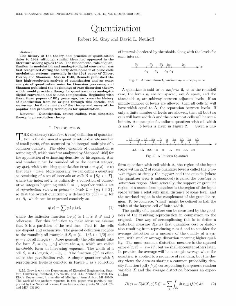
where the indicator function 1S(x) is 1 if x ∈ S and 0otherwise. For this definition to make sense we assumethat S is a partition of the real line. That is, the cellsare disjoint and exhaustive. The general definition reducesto the rounding off example if Si = (i − 1/2, i + 1/2] andyi = i for all integers i. More generally the cells might takethe form Si = (ai−1, ai] where the ai’s, which are calledthresholds, form an increasing sequence. The width of acell Si is its length, ai − ai−1. The function q(x) is oftencalled the quantization rule. A simple quantizer with 5reproduction levels is depicted in Figure 1 as a collection
R.M. Gray is with the Department of Electrical Engineering, Stan-ford University, Stanford, CA 94305, and D.L. Neuhoff is with theEECS Department, University of Michigan, Ann Arbor, MI 48109.The work of the authors reported in this paper was partially sup-ported by the National Science Foundation under grants NCR-941574and MIP-931190.
of intervals bordered by thresholds along with the levels foreach interval.
- xa1 a2 a3 a4
y0∗y1∗
y2∗y3∗
y4∗
Fig. 1. A nonuniform Quantizer: a0 = −∞, a5 =∞
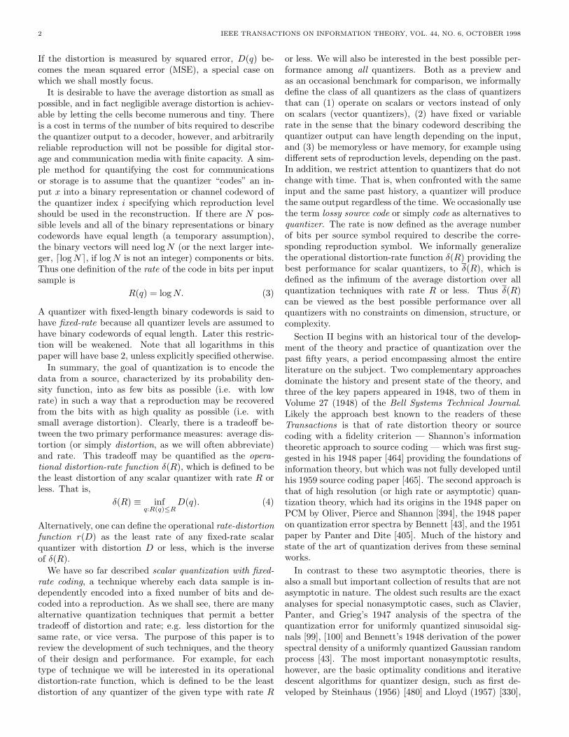
A quantizer is said to be uniform if, as in the roundoffcase, the levels yi are equispaced, say ∆ apart, and thethresholds ai are midway between adjacent levels. If aninfinite number of levels are allowed, then all cells Si willhave width equal to ∆, the separation between levels. Ifonly a finite number of levels are allowed, then all but twocells will have width ∆ and the outermost cells will be semi-infinite. An example of a uniform quantizer with cell width∆ and N = 8 levels is given in Figure 2. Given a uni-
- x∗ ∗ ∗ ∗ ∗ ∗ ∗ ∗ ∗ ∗−4∆−3∆−2∆ −∆ 0 ∆ 2∆ 3∆ 4∆
− 9∆2− 7∆
2− 5∆
2− 3∆
2−∆
2∆2
3∆2
5∆2
7∆2
9∆2
Fig. 2. A Uniform Quantizer
form quantizer with cell width ∆, the region of the inputspace within ∆/2 of some quantizer level is called the gran-ular region or simply the support and that outside (wherethe quantizer error is unbounded) is called the overload orsaturation region. More generally, the support or granularregion of a nonuniform quantizer is the region of the inputspace within a relatively small distance of some level, andthe overload region is the complement of the granular re-gion. To be concrete, “small” might be defined as half thewidth of the largest cell of finite width.
The quality of a quantizer can be measured by the good-ness of the resulting reproduction in comparison to theoriginal. One way of accomplishing this is to define adistortion measure d(x, x) that quantifies cost or distor-tion resulting from reproducing x as x and to consider theaverage distortion as a measure of the quality of a sys-tem, with smaller average distortion meaning higher qual-ity. The most common distortion measure is the squarederror d(x, x) = |x− x|2, but we shall encounter others later.In practice the average will be a sample average when thequantizer is applied to a sequence of real data, but the the-ory views the data as sharing a common probability den-sity function (pdf) f(x) corresponding to a generic randomvariable X and the average distortion becomes an expec-tation
D(q) = E[d(X, q(X))] =∑i
∫Si
d(x, yi)f(x) dx. (2)
2 IEEE TRANSACTIONS ON INFORMATION THEORY, VOL. 44, NO. 6, OCTOBER 1998
If the distortion is measured by squared error, D(q) be-comes the mean squared error (MSE), a special case onwhich we shall mostly focus.
It is desirable to have the average distortion as small aspossible, and in fact negligible average distortion is achiev-able by letting the cells become numerous and tiny. Thereis a cost in terms of the number of bits required to describethe quantizer output to a decoder, however, and arbitrarilyreliable reproduction will not be possible for digital stor-age and communication media with finite capacity. A sim-ple method for quantifying the cost for communicationsor storage is to assume that the quantizer “codes” an in-put x into a binary representation or channel codeword ofthe quantizer index i specifying which reproduction levelshould be used in the reconstruction. If there are N pos-sible levels and all of the binary representations or binarycodewords have equal length (a temporary assumption),the binary vectors will need logN (or the next larger inte-ger, dlogNe, if logN is not an integer) components or bits.Thus one definition of the rate of the code in bits per inputsample is
R(q) = logN. (3)
A quantizer with fixed-length binary codewords is said tohave fixed-rate because all quantizer levels are assumed tohave binary codewords of equal length. Later this restric-tion will be weakened. Note that all logarithms in thispaper will have base 2, unless explicitly specified otherwise.
In summary, the goal of quantization is to encode thedata from a source, characterized by its probability den-sity function, into as few bits as possible (i.e. with lowrate) in such a way that a reproduction may be recoveredfrom the bits with as high quality as possible (i.e. withsmall average distortion). Clearly, there is a tradeoff be-tween the two primary performance measures: average dis-tortion (or simply distortion, as we will often abbreviate)and rate. This tradeoff may be quantified as the opera-tional distortion-rate function δ(R), which is defined to bethe least distortion of any scalar quantizer with rate R orless. That is,
δ(R) ≡ infq:R(q)≤R
D(q). (4)
Alternatively, one can define the operational rate-distortionfunction r(D) as the least rate of any fixed-rate scalarquantizer with distortion D or less, which is the inverseof δ(R).
We have so far described scalar quantization with fixed-rate coding, a technique whereby each data sample is in-dependently encoded into a fixed number of bits and de-coded into a reproduction. As we shall see, there are manyalternative quantization techniques that permit a bettertradeoff of distortion and rate; e.g. less distortion for thesame rate, or vice versa. The purpose of this paper is toreview the development of such techniques, and the theoryof their design and performance. For example, for eachtype of technique we will be interested in its operationaldistortion-rate function, which is defined to be the leastdistortion of any quantizer of the given type with rate R
or less. We will also be interested in the best possible per-formance among all quantizers. Both as a preview andas an occasional benchmark for comparison, we informallydefine the class of all quantizers as the class of quantizersthat can (1) operate on scalars or vectors instead of onlyon scalars (vector quantizers), (2) have fixed or variablerate in the sense that the binary codeword describing thequantizer output can have length depending on the input,and (3) be memoryless or have memory, for example usingdifferent sets of reproduction levels, depending on the past.In addition, we restrict attention to quantizers that do notchange with time. That is, when confronted with the sameinput and the same past history, a quantizer will producethe same output regardless of the time. We occasionally usethe term lossy source code or simply code as alternatives toquantizer. The rate is now defined as the average numberof bits per source symbol required to describe the corre-sponding reproduction symbol. We informally generalizethe operational distortion-rate function δ(R) providing thebest performance for scalar quantizers, to δ(R), which isdefined as the infimum of the average distortion over allquantization techniques with rate R or less. Thus δ(R)can be viewed as the best possible performance over allquantizers with no constraints on dimension, structure, orcomplexity.
Section II begins with an historical tour of the develop-ment of the theory and practice of quantization over thepast fifty years, a period encompassing almost the entireliterature on the subject. Two complementary approachesdominate the history and present state of the theory, andthree of the key papers appeared in 1948, two of them inVolume 27 (1948) of the Bell Systems Technical Journal.Likely the approach best known to the readers of theseTransactions is that of rate distortion theory or sourcecoding with a fidelity criterion — Shannon’s informationtheoretic approach to source coding — which was first sug-gested in his 1948 paper [464] providing the foundations ofinformation theory, but which was not fully developed untilhis 1959 source coding paper [465]. The second approach isthat of high resolution (or high rate or asymptotic) quan-tization theory, which had its origins in the 1948 paper onPCM by Oliver, Pierce and Shannon [394], the 1948 paperon quantization error spectra by Bennett [43], and the 1951paper by Panter and Dite [405]. Much of the history andstate of the art of quantization derives from these seminalworks.
In contrast to these two asymptotic theories, there isalso a small but important collection of results that are notasymptotic in nature. The oldest such results are the exactanalyses for special nonasymptotic cases, such as Clavier,Panter, and Grieg’s 1947 analysis of the spectra of thequantization error for uniformly quantized sinusoidal sig-nals [99], [100] and Bennett’s 1948 derivation of the powerspectral density of a uniformly quantized Gaussian randomprocess [43]. The most important nonasymptotic results,however, are the basic optimality conditions and iterativedescent algorithms for quantizer design, such as first de-veloped by Steinhaus (1956) [480] and Lloyd (1957) [330],
GRAY AND NEUHOFF: QUANTIZATION 3
and later popularized by Max (1960) [349].Our goal in the next section is to introduce in histor-
ical context many of the key ideas of quantization thatoriginated in classical works and evolved over the past 50years, and in the remaining sections to survey selectivelyand in more detail a variety of results which illustrate boththe historical development and the state of the field. Sec-tion III will present basic background material that will beneeded in the remainder of the paper, including the generaldefinition of a quantizer and the basic forms of optimalitycriteria and descent algorithms. Some such material hasalready been introduced and more will be introduced inSection II. However, for completeness, Section III will belargely self-contained. Section IV reviews the developmentof quantization theories and compares the approaches. Fi-nally, Section V describes a number of specific quantizationtechniques.
In any review of a large subject such as quantizationthere is not space to discuss or even mention all work on thesubject. Though we have made an effort to select the mostimportant work, no doubt we have missed some importantwork due to bias, misunderstanding, or ignorance. For thiswe apologize, both to the reader and to the researcherswhose work we may have neglected.
II. History
The history of quantization often takes on several paral-lel paths, which causes some problems in our clustering oftopics. We follow roughly a chronological order within eachand order the paths as best we can. Specifically, we willfirst track the design and analysis of practical quantizationtechniques in three paths: fixed-rate scalar quantization,which leads directly from the discussion of Section I, predic-tive and transform coding, which adds linear processing toscalar quantization in order to exploit source redundancy,and variable-rate quantization, which uses Shannon’s loss-less source coding techniques [464] to reduce rate. (Loss-less codes were originally called noiseless.) Next we followearly forward looking work on vector quantization, includ-ing the seminal work of Shannon and Zador, in which vectorquantization appears more to be a paradigm for analyzingthe fundamental limits of quantizer performance than apractical coding technique. A surprising amount of suchvector quantization theory was developed outside the con-ventional communications and signal processing literature.Subsequently, we review briefly the developments from themid 1970’s to the mid 1980’s which mainly concern theemergence of vector quantization as a practical technique.Finally, we sketch briefly developments from the mid 1980’sto the present. Except where stated otherwise, we presumesquared error as the distortion measure.
A. Fixed-Rate Scalar Quantization: PCM and the Originsof Quantization Theory
Both quantization and source coding with a fidelity cri-terion have their origins in pulse code modulation (PCM),a technique patented in 1938 by Reeves [432], who 25 yearslater wrote an historical perspective on and an appraisal of
the future of PCM with Deloraine [120]. The predictionswere surprisingly accurate as to the eventual ubiquity ofdigital speech and video. The technique was first success-fully implemented in hardware by Black, who reported theprinciples and implementation in 1947 [51], as did anotherBell Labs paper by Goodall [209]. PCM was subsequentlyanalyzed in detail and popularized by Oliver, Pierce, andShannon in 1948 [394]. PCM was the first digital tech-nique for conveying an analog information signal (princi-pally telephone speech) over an analog channel (typically,a wire or the atmosphere). In other words it is a modula-tion technique, i.e., an alternative to AM, FM and variousother types of pulse modulation. It consists of three maincomponents: a sampler (including a prefilter), a quantizer(with a fixed-rate binary encoder) and a binary pulse mod-ulator. The sampler converts a continuous-time waveformx(t) into a sequence of samples xn = x(n/fs), where fsis the sampling frequency. The sampler is ordinarily pre-ceded by a lowpass filter with cutoff frequency fs/2. Ifthe filter is ideal, then the Shannon-Nyquist or Shannon-Whittaker-Kotelnikov sampling theorem ensures that thelowpass filtered signal can, in principle, be perfectly re-covered by appropriately filtering the samples. Quantiza-tion of the samples renders this an approximation, withthe MSE of the recovered waveform being, approximately,the sum of the MSE of the quantizer, D(q), and the highfrequency power removed by the lowpass filter. The binarypulse modulator typically uses the bits produced by thequantizer to determine the amplitude, frequency or phaseof a sinusoidal carrier waveform. In the evolutionary de-velopment of modulation techniques it was found that theperformance of pulse amplitude modulation in the presenceof noise could be improved if the samples were quantizedto the nearest of a set of N levels before modulating thecarrier (64 equally spaced levels was typical). Though thisintroduces quantization error, deciding which of the N lev-els had been transmitted in the presence of noise could bedone with such reliability that the overall MSE was sub-stantially reduced. Reducing the number of quantizationlevels N made it even easier to decide which level had beentransmitted, but came at the cost of a considerable increasein the MSE of the quantizer. A solution was to fix N at avalue giving acceptably small quantizer MSE and to binaryencode the levels, so that the receiver had only to makebinary decisions, something it can do with great reliabil-ity. The resulting system, PCM, had the best resistance tonoise of all modulations of the time.
As the digital era emerged, it was recognized that thesampling, quantizing, and encoding part of PCM performsan analog-to-digital (A/D) conversion, with uses extendingmuch beyond communication over analog channels. Evenin the communications field, it was recognized that the taskof analog-to-digital conversion (and source coding) shouldbe factored out of binary modulation as a separate task.Thus, PCM is now generally considered to just consist ofsampling, quantizing and encoding; i.e., it no longer in-cludes the binary pulse modulation.
Although quantization in the information theory litera-
4 IEEE TRANSACTIONS ON INFORMATION THEORY, VOL. 44, NO. 6, OCTOBER 1998
ture is generally considered as a form of data compression,its use for modulation or A/D conversion was originallyviewed as data expansion or, more accurately, bandwidthexpansion. For example, a speech waveform occupyingroughly 4kHz would have a Nyquist rate of 8kHz. Sam-pling at the Nyquist rate and quantizing at 8 bits per sam-ple and then modulating the resulting binary pulses usingamplitude or frequency shift keying would yield a signaloccupying roughly 64kHz, a 16 fold increase in bandwidth!Mathematically this constitutes compression in the sensethat a continuous waveform requiring an infinite numberof bits is reduced to a finite number of bits, but for practi-cal purposes PCM is not well interpreted as a compressionscheme.
In an early contribution to the theory of quantization,Clavier, Panter, and Grieg (1947) [99], [100] applied Rice’scharacteristic function or transform method [434] to pro-vide exact expressions for the quantization error and itsmoments resulting from uniform quantization for certainspecific inputs, including constants and sinusoids. Thecomplicated sums of Bessel functions resembled the earlyanalyses of another nonlinear modulation technique, FM,and left little hope for general closed form solutions forinteresting signals.
The first general contributions to quantization theorycame in 1948 with the papers of Oliver, Pierce, and Shan-non [394] and Bennett [43]. As part of their analysis ofPCM for communications, they developed the oft-quotedresult that for large rate or resolution, a uniform quantizerwith cell width ∆ yields average distortion D(q) ∼= ∆2/12.If the quantizer has N levels and rate R = logN , and thesource has input range (or support) of width A, so that∆ = A/N is the natural choice, then the ∆2/12 approxi-mation yields the familiar form for the signal-to-noise ratio(SNR) of
10 log10
var(X)E[(q(X)−X)2]
= c+ 20R log10 2
∼= c+ 6R dB
showing that for large rate, the SNR of uniform quantiza-tion increases 6 dB for each one bit increase of rate, whichis often referred to as the “6 dB per bit rule”. The ∆2/12formula is considered a high-resolution formula, indeed thefirst such formula, in that it applies to the situation wherethe cells and average distortion are small, and the rate islarge, so that the reproduction produced by the quantizeris quite accurate. The ∆2/12 result also appeared manyyears earlier (albeit in somewhat disguised form) in Shep-pard’s 1898 treatment [468].
Bennett also developed several other fundamental resultsin quantization theory. He generalized the high-resolutionapproximation for uniform quantization to provide an ap-proximation to D(q) for companders, systems that pre-ceded a uniform quantizer by a monotonic smooth non-linearity called a “compressor,” say G, and used the in-verse nonlinearity when reconstructing the signal. Thusthe output reproduction x given an input x was given by
x = G−1(q(G(x)), where q is a uniform quantizer. Bennettshowed that in this case
D(q) ∼= ∆2
12
∫f(x)g2(x)
dx, (5)
where g(x) = dG(x)/dx, ∆ is the cell width of the uniformquantizer, and the integral is taken over the granular rangeof the input. (The constant 1/12 in the above assumesthat G maps to the unit interval [0,1].) Since, as Bennettpointed out, any nonuniform quantizer can be implementedas a compander, this result, often referred to as “Bennett’sintegral,” provides an asymptotic approximation for anyquantizer. It is useful to jump ahead and point out that gcan be interpreted, as Lloyd would explicitly point out in1957 [330], as a constant times a “quantizer point-densityfunction λ(x),” that is, a function with the property thatfor any region S
number of quantizer levels in S ≈ N∫S
λ(x) dx. (6)
Since integrating λ(x) over a region gives the fraction ofquantizer reproduction levels in the region, it is evidentthat λ(x) is normalized so that
∫< λ(x) dx = 1. It will also
prove useful to consider the unnormalized quantizer pointdensity Λ(x), which when integrated over S gives the totalnumber of levels within S rather than the fraction. Inthe current situation Λ(x) = Nλ(x), but the unnormalizeddensity will generalize to the case where N is infinite.
Rewriting Bennett’s integral in terms of the point-density function yields its more common form
D(q) ∼= 112
1N2
∫f(x)λ2(x)
dx. (7)
The idea of a quantizer point-density function will gener-alize to vectors, while the compander approach will not inthe sense that not all vector quantizers can be representedas companders [192].
Bennett also demonstrated that, under assumptions ofhigh resolution and smooth densities, the quantizationerror behaved much like random “noise”: it had smallcorrelation with the signal and had approximately a flat(“white”) spectrum. This led to an “additive noise” modelof quantizer error, since with these properties the formulaq(X) = X + [q(X)−X] could be interpreted as represent-ing the quantizer output as the sum of a signal and whitenoise. This model was later popularized by Widrow [528],[529], but the viewpoint avoids the fact that the “noise”is in fact dependent on the signal and the approximationsare valid only under certain conditions. Signal independentquantization noise has generally been found to be percep-tually desirable. This was the motivation for randomizingthe action of quantization by the addition of a dither signal,a method introduced by Roberts [442] as a means of mak-ing quantized images look better by replacing the artifactsresulting from deterministic errors by random noise. Weshall return to dithering in Section V, where it will be seenthat suitable dithering can indeed make exact the Bennett
GRAY AND NEUHOFF: QUANTIZATION 5
approximations of uniform distribution and signal indepen-dence of the overall quantizer noise. Bennett also used avariation of Rice’s method to derive an exact computationof the spectrum of quantizer noise when a Gaussian processis uniformly quantized, providing one of the very few exactcomputations of quantization error spectra.
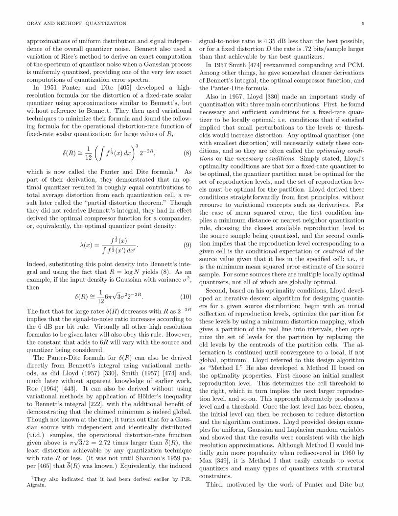
In 1951 Panter and Dite [405] developed a high-resolution formula for the distortion of a fixed-rate scalarquantizer using approximations similar to Bennett’s, butwithout reference to Bennett. They then used variationaltechniques to minimize their formula and found the follow-ing formula for the operational distortion-rate function offixed-rate scalar quantization: for large values of R,
δ(R) ∼= 112
(∫f
13 (x) dx
)3
2−2R, (8)
which is now called the Panter and Dite formula.1 Aspart of their derivation, they demonstrated that an op-timal quantizer resulted in roughly equal contributions tototal average distortion from each quantization cell, a re-sult later called the “partial distortion theorem.” Thoughthey did not rederive Bennett’s integral, they had in effectderived the optimal compressor function for a compander,or, equivalently, the optimal quantizer point density:
λ(x) =f
13 (x)∫
f13 (x′) dx′
. (9)
Indeed, substituting this point density into Bennett’s inte-gral and using the fact that R = logN yields (8). As anexample, if the input density is Gaussian with variance σ2,then
δ(R) ∼= 112
6π√
3σ22−2R. (10)
The fact that for large rates δ(R) decreases with R as 2−2R
implies that the signal-to-noise ratio increases according tothe 6 dB per bit rule. Virtually all other high resolutionformulas to be given later will also obey this rule. However,the constant that adds to 6R will vary with the source andquantizer being considered.
The Panter-Dite formula for δ(R) can also be deriveddirectly from Bennett’s integral using variational meth-ods, as did Lloyd (1957) [330], Smith (1957) [474] and,much later without apparent knowledge of earlier work,Roe (1964) [443]. It can also be derived without usingvariational methods by application of Holder’s inequalityto Bennett’s integral [222], with the additional benefit ofdemonstrating that the claimed minimum is indeed global.Though not known at the time, it turns out that for a Gaus-sian source with independent and identically distributed(i.i.d.) samples, the operational distortion-rate functiongiven above is π
√3/2 = 2.72 times larger than δ(R), the
least distortion achievable by any quantization techniquewith rate R or less. (It was not until Shannon’s 1959 pa-per [465] that δ(R) was known.) Equivalently, the induced
1They also indicated that it had been derived earlier by P.R.Aigrain.
signal-to-noise ratio is 4.35 dB less than the best possible,or for a fixed distortion D the rate is .72 bits/sample largerthan that achievable by the best quantizers.
In 1957 Smith [474] reexamined companding and PCM.Among other things, he gave somewhat cleaner derivationsof Bennett’s integral, the optimal compressor function, andthe Panter-Dite formula.
Also in 1957, Lloyd [330] made an important study ofquantization with three main contributions. First, he foundnecessary and sufficient conditions for a fixed-rate quan-tizer to be locally optimal; i.e. conditions that if satisfiedimplied that small perturbations to the levels or thresh-olds would increase distortion. Any optimal quantizer (onewith smallest distortion) will necessarily satisfy these con-ditions, and so they are often called the optimality condi-tions or the necessary conditions. Simply stated, Lloyd’soptimality conditions are that for a fixed-rate quantizer tobe optimal, the quantizer partition must be optimal for theset of reproduction levels, and the set of reproduction lev-els must be optimal for the partition. Lloyd derived theseconditions straightforwardly from first principles, withoutrecourse to variational concepts such as derivatives. Forthe case of mean squared error, the first condition im-plies a minimum distance or nearest neighbor quantizationrule, choosing the closest available reproduction level tothe source sample being quantized, and the second condi-tion implies that the reproduction level corresponding to agiven cell is the conditional expectation or centroid of thesource value given that it lies in the specified cell; i.e., itis the minimum mean squared error estimate of the sourcesample. For some sources there are multiple locally optimalquantizers, not all of which are globally optimal.
Second, based on his optimality conditions, Lloyd devel-oped an iterative descent algorithm for designing quantiz-ers for a given source distribution: begin with an initialcollection of reproduction levels, optimize the partition forthese levels by using a minimum distortion mapping, whichgives a partition of the real line into intervals, then opti-mize the set of levels for the partition by replacing theold levels by the centroids of the partition cells. The al-ternation is continued until convergence to a local, if notglobal, optimum. Lloyd referred to this design algorithmas “Method I.” He also developed a Method II based onthe optimality properties. First choose an initial smallestreproduction level. This determines the cell threshold tothe right, which in turn implies the next larger reproduc-tion level, and so on. This approach alternately produces alevel and a threshold. Once the last level has been chosen,the initial level can then be rechosen to reduce distortionand the algorithm continues. Lloyd provided design exam-ples for uniform, Gaussian and Laplacian random variablesand showed that the results were consistent with the highresolution approximations. Although Method II would ini-tially gain more popularity when rediscovered in 1960 byMax [349], it is Method I that easily extends to vectorquantizers and many types of quantizers with structuralconstraints.
Third, motivated by the work of Panter and Dite but
6 IEEE TRANSACTIONS ON INFORMATION THEORY, VOL. 44, NO. 6, OCTOBER 1998
apparently unaware of that of Bennett or Smith, Lloydrederived Bennett’s integral and the Panter-Dite formulabased on the concept of point-density function. This wasa critically important step for subsequent generalizationsof Bennett’s integral to vector quantizers. He also showeddirectly that in situations where the global optimum is theonly local optimum, quantizers that satisfy the optimalityconditions have, asymptotically, the optimal point densitygiven by (9).
Unfortunately Lloyd’s work was not published in anarchival journal at the time. Instead, it was presented atthe 1957 Institute of Mathematical Statistics (IMS) meet-ing and appeared in print only as a Bell Laboratories Tech-nical Memorandum. As a result, its results were not widelyknown in the engineering literature for many years, andmany were independently rediscovered. All of the indepen-dent rediscoveries, however, used variational derivations,rather than Lloyd’s simple derivations. The latter were es-sential for later extensions to vector quantizers and to thedevelopment of many quantizer optimization procedures.To our knowledge, the first mention of Lloyd’s work inthe IEEE literature came in 1964 with Fleischer’s [170]derivation of a sufficient condition (namely, that the logof the source density be concave) in order that the optimalquantizer be the only locally optimal quantizer, and con-sequently, that Lloyd’s Method I yields a globally optimalquantizer. (The condition is satisfied for common densitiessuch as Gaussian and Laplacian.) Zador [561] had referredto Lloyd a year earlier in his Ph.D. thesis, to be discussedlater.
Later in the same year in another Bell Telephone Labora-tories Technical Memorandum, Goldstein [207] used vari-ational methods to derive conditions for global optimal-ity of a scalar quantizer in terms of second order partialderivatives with respect to the quantizer levels and thresh-olds. He also provided a simple counterintuitive exampleof a symmetric density for which the optimal quantizer wasasymmetric.
In 1959 Shtein [471] added terms representing overloaddistortion to the ∆2/12 formula and to Bennett’s inte-gral and used them to optimize uniform and nonuniformquantizers. Unaware of prior work except for Bennett’s,he rederived the optimal compressor characteristic and thePanter-Dite formula.
In 1960 Max [349] published a variational proof of theLloyd optimality properties for rth power distortion mea-sures, rediscovered Lloyd’s Method II, and numerically in-vestigated the design of fixed-rate quantizers for a varietyof input densities.
Also in 1960, Widrow [529] derived an exact formula forthe characteristic function of a uniformly quantized signalwhen the quantizer has an infinite number of levels. Hisresults showed that under the condition that the character-istic function of the input signal be zero when its argumentis greater than π/∆, the moments of the quantized randomvariable are the same as the moments of the signal plusan additive signal-independent random variable uniformlydistributed on (−∆/2,∆/2]. This has often been misinter-
preted as saying that the quantized random variable can beapproximated as being the input plus signal-independentuniform noise, a clearly false statement since the quantizererror q(X) − X is a deterministic function of the signal.The “bandlimited” property of the characteristic functionimplies from Fourier transform theory that the probabilitydensity function must have infinite support since a signaland its transform cannot both be perfectly bandlimited.
We conclude this subsection by mentioning early workthat appeared in the mathematical and statistical litera-ture and which, in hindsight, can be viewed as related toscalar quantization. Specifically, in 1950-1951 Dalenius etal. [118], [119] used variational techniques to consider op-timal grouping of Gaussian data with respect to averagesquared error. Lukaszewicz and H. Steinhaus [336] (1955)developed what we now consider to be the Lloyd optimal-ity conditions using variational techniques in a study ofoptimum go/no-go gauge sets (as acknowledged by Lloyd).Cox in 1957 [111] also derived similar conditions. Someadditional early work, which can now be seen as relatingto vector quantization, will be reviewed later [480], [159],[561].
B. Scalar Quantization with Memory
It was recognized early that common sources such asspeech and images had considerable “redundancy” thatscalar quantization could not exploit. The term “redun-dancy” was commonly used in the early days and is stillpopular in some of the quantization literature. Strictlyspeaking it refers to the statistical correlation or depen-dence between the samples of such sources and is usuallyreferred to as memory in the information theory literature.As our current emphasis is historical, we follow the tra-ditional language. While not disrupting the performanceof scalar quantizers, such redundancy could be exploitedto attain substantially better rate-distortion performance.The early approaches toward this end combined linear pro-cessing with scalar quantization, thereby preserving thesimplicity of scalar quantization while using intuition-basedarguments and insights to improve performance by incor-porating memory into the overall code. The two most im-portant approaches of this variety were predictive codingand transform coding. A shared intuition was that a pre-processing operation intended to make scalar quantizationmore efficient should “remove the redundancy” in the data.Indeed, to this day there is a common belief that data com-pression is equivalent to redundancy removal and that datawithout redundancy cannot be further compressed. As willbe discussed later, this belief is contradicted both by Shan-non’s work, which demonstrated strictly improved perfor-mance using vector quantizers even for memoryless sources,and by the early work of Fejes Toth (1959) [159]. Neverthe-less, removing redundancy leads to much improved codes.
Predictive quantization appears to originate in the 1946delta modulation patent of Derjavitch, Deloraine, and VanMierlo [129], but the most commonly cited early referencesare Cutler’s patent [117] 2,605,361 on “Differential quanti-zation of communication signals” and on DeJager’s Philips
GRAY AND NEUHOFF: QUANTIZATION 7
technical report on delta modulation [128]. Cutler statedin his patent that it “is the object of the present inven-tion to improve the efficiency of communication systemsby taking advantage of correlation in the signals of thesesystems” and Derjavitch et al. also cited the reductionof redundancy as the key to the reduction of quantizationnoise. In 1950 Elias [141] provided an information theoreticdevelopment of the benefits of predictive coding, but thework was not published until 1955 [142]. Other early refer-ences include [395], [300], [237], [511], [572]. In particular,[511] claims Bennett-style asymptotics for high resolutionquantization error, but as will be discussed later such ap-proximations have yet to be rigorously derived.
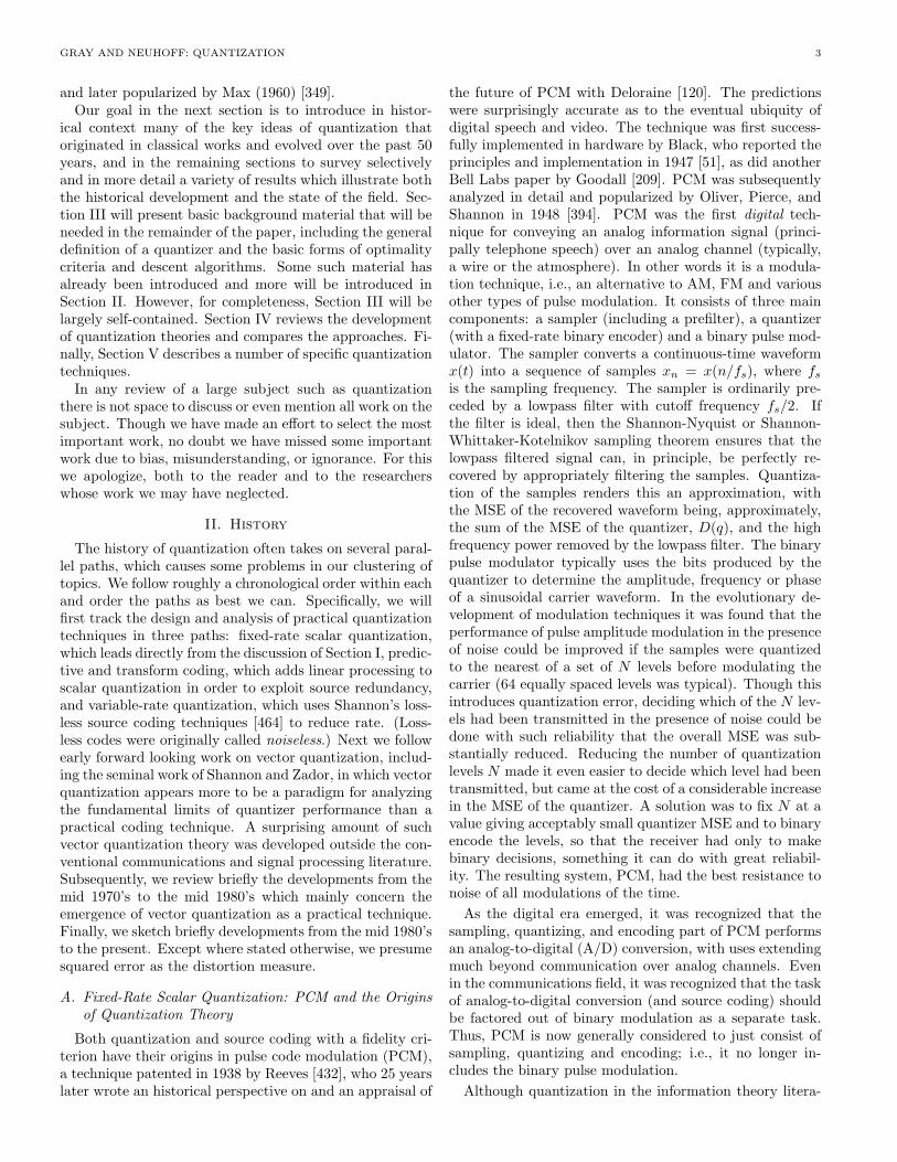
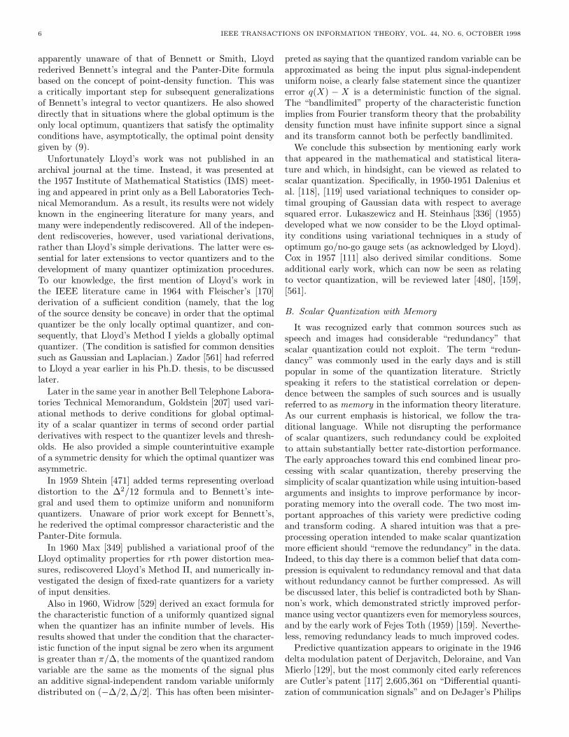
¿From the point of view of least squares estimation the-ory, if one were to optimally predict a data sequence basedon its past in the sense of minimizing the mean squarederror, then the resulting error or residual or innovations se-quence would be uncorrelated and it would have the min-imum possible variance. To permit reconstruction in acoded system, however, the prediction must be based onpast reconstructed samples and not true samples. Thisis accomplished by placing a quantizer inside a predictionloop and using the same predictor to decode the signal. Asimple predictive quantizer or differential pulse coded mod-ulator (DPCM) is depicted in Figure 3. If the predictor issimply the last sample and the quantizer has only one bit,the system becomes a delta-modulator. Predictive quantiz-ers are considered to have memory in that the quantizationof a sample depends on previous samples, via the feedbackloop.
Xn- l++
6Xn
−-
enQ
en
-in BinaryEncoder
-
l++
Xn
?+-
P �
Encoder
- BinaryDecoder
in- Q−1 -en l+ -Xn
�P
6Xn
+
+
Decoder
Fig. 3. Predictive Quantizer Encoder/Decoder
Predictive quantizers have been extensively developed,for example there are many adaptive versions, and arewidely used in speech and video coding, where a numberof standards are based on them. In speech coding theyform the basis of ITU-G.721, 722, 723, and 726, and invideo coding they form the basis of the interframe cod-ing schemes standardized in the MPEG and H.26X series.Comprehensive discussions may be found in books [265],[374], [196], [424], [50], [458] and survey papers [264], [198].
Though decorrelation was an early motivation for predic-tive quantization, the most common view at present is thatthe primary role of the predictor is to reduce the varianceof the variable to be scalar quantized. This view stemsfrom the facts that (a) it is the prediction errors ratherthan the source samples that are quantized, (b) the over-all quantization error precisely equals that of the scalarquantizer operating on the prediction errors, (c) the op-erational distortion-rate function δ(R) for scalar quantiza-tion is proportional to variance (more precisely, a scalingof the random variable being quantized by a factor a re-sults in a scaling of δ(R) by a2), and (d) the density ofthe prediction error is usually sufficiently similar in formto that of the source that its operational distortion-ratefunction is smaller than that of the original source by, ap-proximately, the ratio of the variance of the source to thatof the prediction error, a quantity that is often called aprediction gain [350], [396], [482], [397], [265]. Analysesof this form usually claim that under high-resolution con-ditions the distribution of the prediction error approachesthat of the error when predictions are based on past sourcesamples rather than past reproductions. However, it is notclear that the accuracy of this approximation increases suf-ficiently rapidly with finer resolution to ensure that the dif-ference between the operational distortion-rate functions ofthe two types of prediction errors is small relative to theirvalues, which are themselves decreasing as the resolutionbecomes finer. Indeed, it is still an open question whetherthis type of analysis, which typically uses Bennett andPanter-Dite formulas, is asymptotically correct. Neverthe-less, the results of such high-resolution approximations arewidely accepted and often compare well with experimentalresults [265], [156]. Assuming that they give the correct an-swer, then for large rates and a stationary, Gaussian sourcewith memory, the distortion of an optimized DPCM quan-tizer is less than that of a scalar quantizer by the factorσ2
1/σ2, where σ2 is the variance of the source and σ2
1 is theone-step prediction error; i.e. the smallest MSE of any pre-diction of one sample based on previous samples. It turnsout that this exceeds δ(R) by the same factor by which thedistortion of optimal fixed-rate scalar quantization exceedsδ(R) for a memoryless Gaussian source. Hence, it appearsthat DPCM does a good job of exploiting source memorygiven that it is based on scalar quantization, at least underthe high-resolution assumption.
Because it has not been rigorously shown that one mayapply Bennett’s integral or the Panter-Dite formula di-rectly to the prediction error, the analysis of such feedbackquantization systems has proved to be notoriously diffi-cult, with results limited to proofs of stability [191], [281],[284], i.e. asymptotic stationarity, to analyses of distor-tion via Hermite polynomial expansions for Gaussian pro-cesses [124], [473], [17], [346], [241], [262], [156], [189], [190],[367], [368], [369], [293], to analyses of distortion when thesource is a Wiener process [163], [346], [240], and to ex-act solutions of the nonlinear difference equations describ-ing the system and hence to descriptions of the output se-quences and their moments, including power spectral den-
8 IEEE TRANSACTIONS ON INFORMATION THEORY, VOL. 44, NO. 6, OCTOBER 1998
X
X1
X2
Xk
-
-
...
-
T
Y
-
-
-
q1
q2
...
qk
Y
-
-
-
T−1
-
-
...
-
X1
X2
Xk
X
Fig. 4. Transform Code
sities, for constant and sinusoidal signals and finite sumsof sinusoids using Rice’s method, results which extend thework of Panter, Clavier and Grieg to quantizers inside afeedback loop [260], [71], [215], [216], [72]. Conditions foruse in code design resembling the Lloyd optimality con-ditions have been studied for feedback quantization [161],[203], [41], but the conditions are not optimality conditionsin the Lloyd sense, i.e., they are not necessary conditionsfor a quantizer within a feedback loop to yield the mini-mum average distortion subject to a rate constraint. Wewill return to this issue when we consider finite-state vec-tor quantizers. There has also been work on the optimalityof certain causal coding structures somewhat akin to pre-dictive or feedback quantization [331], [414], [148], [534],[178], [381], [521].
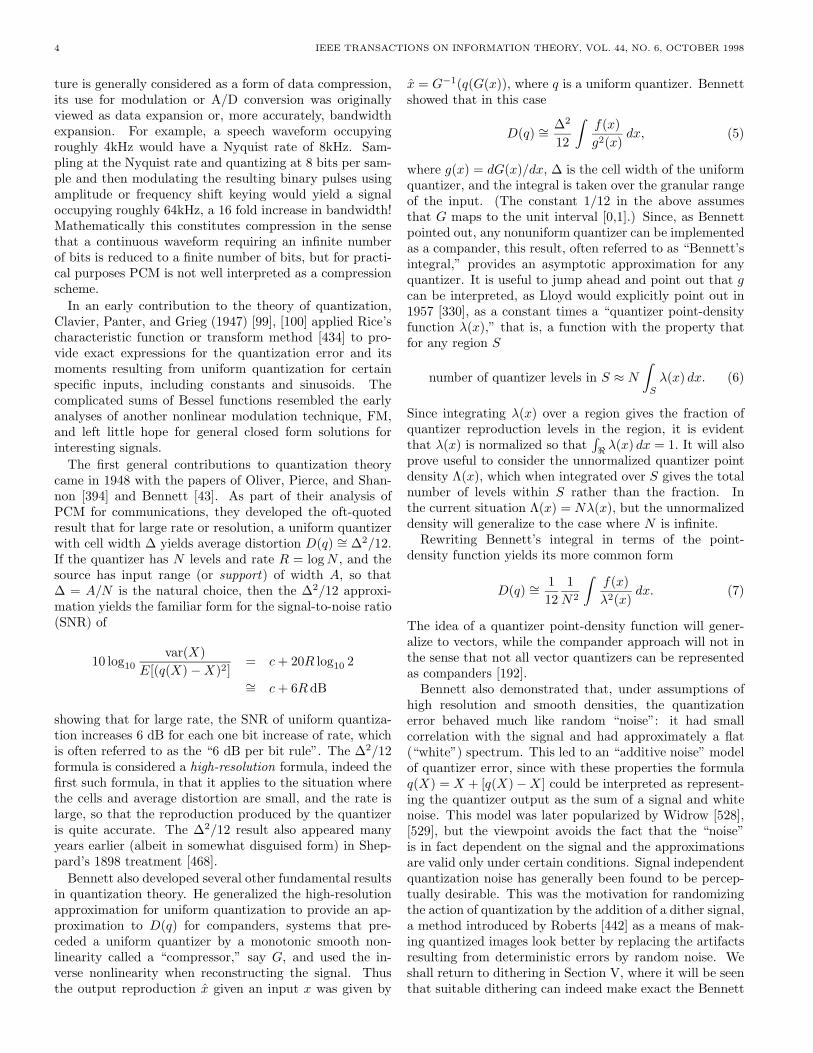
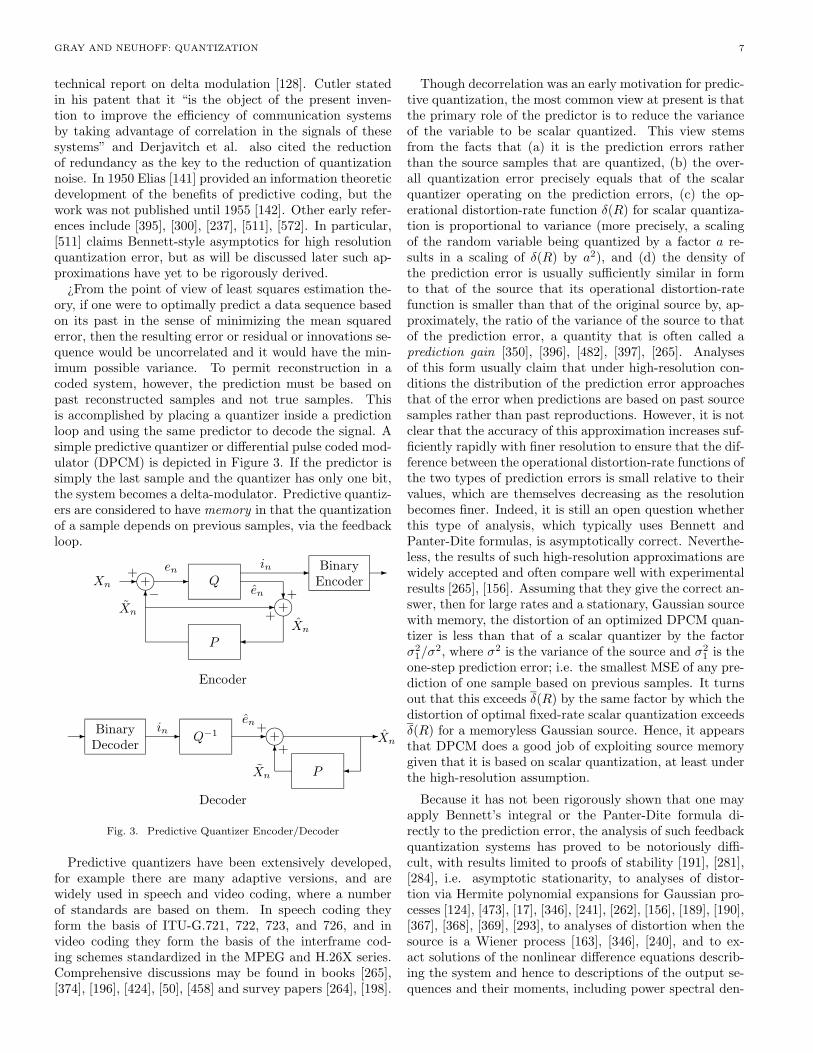
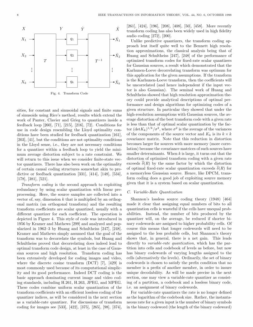
Transform coding is the second approach to exploitingredundancy by using scalar quantization with linear pre-processing. Here, the source samples are collected into avector of, say, dimension k that is multiplied by an orthog-onal matrix (an orthogonal transform) and the resultingtransform coefficients are scalar quantized, usually with adifferent quantizer for each coefficient. The operation isdepicted in Figure 4. This style of code was introduced in1956 by Kramer and Mathews [299] and analyzed and pop-ularized in 1962–3 by Huang and Schultheiss [247], [248].Kramer and Mathews simply assumed that the goal of thetransform was to decorrelate the symbols, but Huang andSchultheiss proved that decorrelating does indeed lead tooptimal transform code design, at least in the case of Gaus-sian sources and high resolution. Transform coding hasbeen extensively developed for coding images and video,where the discrete cosine transform (DCT) [7], [429] ismost commonly used because of its computational simplic-ity and its good performance. Indeed DCT coding is thebasic approach dominating current image and video cod-ing standards, including H.261, H.263, JPEG, and MPEG.These codes combine uniform scalar quantization of thetransform coefficients with an efficient lossless coding of thequantizer indices, as will be considered in the next sectionas a variable-rate quantizer. For discussions of transformcoding for images see [533], [422], [375], [265], [98], [374],
[261], [424], [196], [208], [408], [50], [458]. More recentlytransform coding has also been widely used in high fidelityaudio coding [272], [200].
Unlike predictive quantizers, the transform coding ap-proach lent itself quite well to the Bennett high resolu-tion approximations, the classical analysis being that ofHuang and Schultheiss [247], [248] of the performance ofoptimized transform codes for fixed-rate scalar quantizersfor Gaussian sources, a result which demonstrated that theKarhunen-Loeve decorrelating transform was optimum forthis application for the given assumptions. If the transformis the Karhunen-Loeve transform, then the coefficients willbe uncorrelated (and hence independent if the input vec-tor is also Gaussian). The seminal work of Huang andSchultheiss showed that high resolution approximation the-ory could provide analytical descriptions of optimal per-formance and design algorithms for optimizing codes of agiven structure. In particular they showed that under thehigh-resolution assumptions with Gaussian sources, the av-erage distortion of the best transform code with a given rateis less than that of optimal scalar quantization by the fac-tor (detKk)1/k/σ2, where σ2 is the average of the variancesof the components of the source vector and Kk is its k× kcovariance matrix. Note that this reduction in distortionbecomes larger for sources with more memory (more corre-lation) because the covariance matrices of such sources havesmaller determinants. When k is large, it turns out that thedistortion of optimized transform coding with a given rateexceeds δ(R) by the same factor by which the distortionof optimal fixed-rate scalar quantization exceeds δ(R) fora memoryless Gaussian source. Hence, like DPCM, trans-form coding does a good job of exploiting source memorygiven that it is a system based on scalar quantization.
C. Variable-Rate Quantization
Shannon’s lossless source coding theory (1948) [464]made it clear that assigning equal numbers of bits to allquantization cells is wasteful if the cells have unequal prob-abilities. Instead, the number of bits produced by thequantizer will, on the average, be reduced if shorter bi-nary codewords are assigned to higher probability cells. Ofcourse this means that longer codewords will need to beassigned to the less probable cells, but Shannon’s theoryshows that, in general, there is a net gain. This leadsdirectly to variable-rate quantization, which has the par-tition into cells and codebook of levels as before, but nowhas binary codewords of varying lengths assigned to thecells (alternatively the levels). Ordinarily, the set of binarycodewords is chosen to satisfy the prefix condition that nomember is a prefix of another member, in order to insureunique decodability. As will be made precise in the nextsection, one may view a variable-rate quantizer as consist-ing of a partition, a codebook and a lossless binary code,i.e. an assignment of binary codewords.
For variable-rate quantizers the rate is no longer definedas the logarithm of the codebook size. Rather, the instanta-neous rate for a given input is the number of binary symbolsin the binary codeword (the length of the binary codeword)
GRAY AND NEUHOFF: QUANTIZATION 9
and the rate is the average length of the binary codewords,where the average is taken over the probability distribu-tion of the source samples. The operational distortion-rate function δ(R) using this definition is the smallest av-erage distortion over all (variable-rate) quantizers havingrate R or less. Since we have weakened the constraint byexpanding the allowed set of quantizers, this operationaldistortion-rate function will ordinarily be smaller than thefixed-rate optimum.
Huffman’s algorithm [251] provides a systematic methodof designing binary codes with the smallest possible averagelength for a given set of probabilities, such as those of thecells. Codes designed in this way are typically called Huff-man codes. Unfortunately, there is no known expressionfor the resulting minimum average length in terms of theprobabilities. However, Shannon’s lossless source codingtheorem implies that given a source and a quantizer par-tition, one can always find an assignment of binary code-words (indeed a prefix set) with average length not morethan H(q(X))+1, and that no uniquely decodable set of bi-nary codewords can have average length less than H(q(X)),where
H(q(X)) = −∑i
Pi logPi
is the Shannon entropy of the quantizer output and Pi =Pr(X ∈ Si) is the probability that the source sample Xlies in the ith cell Si. Shannon also provided a simple wayof attaining performance within the upper bound: if thequantizer index is i, then assign it a binary codeword withlength d− logPie (the Kraft inequality ensures that thisis always possible by simply choosing paths in a binarytree). Moreover, tighter bounds have been developed. Forexample Gallager [181] has shown that the entropy can beat most Pmax+.0861 smaller than the average length of theHuffman code, when Pmax, the largest of the Pi’s, is lessthan 1/2. See [73] for discussion of this and other bounds.Since Pmax is ordinarily much smaller than 1/2, this showsthat H(q(X)) is generally a fairly accurate estimate of theaverage rate, especially in the high-resolution case.
Since there is no simple formula determining the rate ofthe Huffman code, but entropy provides a useful estimate,it is reasonable to simplify the variable-length quantizer de-sign problem a little by redefining the instantaneous rateof a variable-rate quantizer as − logPi for the ith quan-tizer level and hence to define the average rate as H(q(X)),the entropy of its output. As mentioned above, this un-derestimates the true rate by a small amount that in nocase exceeds one. We could again define an operationaldistortion-rate function as the minimum average distor-tion over all variable-rate quantizers with output entropyH(q(X)) ≤ R. Since the quantizer output entropy is alower bound to actual rate, this operational distortion-ratefunction may be optimistic; i.e., it falls below δ(R) definedusing average length as rate. A quantizer designed to pro-vide the smallest average distortion subject to an entropyconstraint is called an entropy-constrained scalar quantizer.
Variable-rate quantization is also called variable-lengthquantization or quantization with entropy coding. We
will not, except where critical, take pains to distinguishentropy-constrained quantizers and entropy-coded quantiz-ers. And we will usually blur the distinction between av-erage length and entropy as measures of the rate of suchquantizers unless, again, it is important in some particulardiscussion. This is much the same sort of blurring as usinglogN instead of dlogNe as the measure of rate in fixed-ratequantization.
It is important to note that the number of quantizationcells or levels does not play a primary role in variable-ratequantization because, for example, there can be many levelsin places where the source density is small with little effecton either distortion or rate. Indeed the number of levelscan be infinite, which has the advantage of eliminating theoverload region and resulting overload distortion.
A potential drawback of variable-rate quantization is thenecessity of dealing with the variable numbers of bits thatit produces. For example, if the bits are to be communi-cated through a fixed-rate digital channel, one will have touse buffering and to take buffer overflows and underflowsinto account. Another drawback is the potential for errorpropagation when bits are received by the decoder in error.
The most basic and simple example of a variable-ratequantizer, and one which plays a fundamental role as abenchmark for comparison, is a uniform scalar quantizerwith a variable-length binary lossless code.
The possibility of applying variable-length coding toquantization may well have occurred to any number of peo-ple who were familiar with both quantization and Shan-non’s 1948 paper. The earliest references to such that wehave found are in the 1952 papers by Oliver [395] and Kret-zmer [300]. In 1960, Max [349] had such in mind when hecomputed the entropy of nonuniform and uniform quan-tizers that had been designed to minimize distortion for agiven number of levels. For a Gaussian source his resultsshow that variable-length coding would yield rate reduc-tions of about 0.5 bits/sample.
High-resolution analysis of variable-rate quantization de-veloped in a handful of papers from 1958 to 1968. However,since these papers were widely scattered or unpublished, itwas not until 1968 that the situation was well understoodin the IEEE community.
The first high-resolution analysis was that of Schutzen-berger (1958) [462] who showed that the distortion of opti-mized variable-rate quantization (both scalar and vector)decreases with rate as 2−2R, just as with fixed-rate quanti-zation. But he did not find the multiplicative factors, nordid he describe the nature of the partitions and codebooksthat are best for variable-rate quantization.
In 1959, Renyi [433] showed that a uniform scalar quan-tizer with infinitely many levels and small cell width ∆ hasoutput entropy given approximately by
H(q(X)) ∼= h(X)− log ∆ (11)
whereh(X) = −
∫f(x) log f(x)dx
is the differential entropy of the source variable X.”
10 IEEE TRANSACTIONS ON INFORMATION THEORY, VOL. 44, NO. 6, OCTOBER 1998
In 1963, Koshelev [579] discovered the very interestingfact that in the high-resolution case, the mean-squared er-ror of uniform scalar quantization exceeds that of the leastdistortion achievable by any quantization scheme whatso-ever, i.e. δ(R), by a factor of only πe/6 = 1.42. Equiv-alently, the induced signal-to-noise ratio is only 1.53 dBless than the best possible, or for a fixed distortion D, therate is only 0.255 bit/sample larger than that achievableby the best quantizers. (For the Gaussian source, it gains2.82 dB or 0.47 bit/sample over the best fixed-rate scalarquantizer.) It is also of interest to note that this was thefirst paper to compare the performance of a specific quan-tization scheme to δ(R). Unfortunately, Koshelev’s paperwas published in a journal that was not widely circulated.
In an unpublished 1966 Bell Telephone LaboratoriesTehnical Memo [562], Zador also studied variable-rate (aswell as fixed-rate) quantization. As his focus was on vec-tor quantization, his work will be described later. Here weonly point out that for variable-rate scalar quantizationwith large rate, his results showed that the operationaldistortion-rate function (i.e. the least distortion of suchcodes with a given rate) is
δ(R) ∼= 112
22h(X)2−2R. (12)
Though he was not aware of it, this turns out to be theformula found by Koshelev, thereby demonstrating that inthe high-resolution case, uniform is the best type of scalarquantizer when variable-rate coding is applied.
Finally, in 1967 and 1968 two papers appeared in theIEEE literature (in fact in these Transactions) on variable-rate quantization, without reference to any of the afore-mentioned work. The first, by Goblick and Holsinger [205],showed by numerical evaluation that uniform scalar quan-tization with variable-rate coding attains performancewithin about 1.5 dB (or 0.25 bit/sample) of the best possi-ble for an i.i.d. Gaussian source. The second, by Gish andPierce [204], demonstrated analytically what the first pa-per had found empirically. Specifically, it derived (11) and,more generally, the fact that a high resolution nonuniformscalar quantizer has output entropy
H(q(X)) ∼= h(X) +∫f(x) log Λ(x) dx, (13)
where Λ(x) is the unnormalized point density of the quan-tizer. They then used these approximations along withBennett’s integral to rederive (12) and to show that in thehigh-resolution case, uniform scalar quantizers achieve theoperational distortion-rate function of variable-rate quanti-zation. Next, by comparing to what is called the Shannonlower bound to δ(R), they showed that for i.i.d. sources,the latter is only 1.53 dB (0.255 bits/sample) from thebest possible performance δ(R) of any quantization systemwhatsoever, which is what Koshelev [579] found earlier.Their results showed that such good performance was at-tainable for any source distribution, not just the Gaussiancase checked by Goblick and Holsinger. They also gener-alized the results from squared-error distortion to nonde-creasing functions of magnitude error.
Less well known is their proof of the fact that in thehigh resolution case, the entropy of k successive outputs ofa uniformly scalar quantized stationary source, e.g. withmemory, is
H(q(X1), . . . , q(Xk)) ∼= h(X1, . . . , Xk)− log ∆. (14)
They used this, and the generalization of (13) to vectors, toshow that when rate and k are large, uniform scalar quanti-zation with variable-length coding of k successive quantizeroutputs (block entropy coding) achieves performance thatis 1.53 dB (0.255 bits/sample) from δ(R), even for sourceswith memory. (They accomplished this by comparing toShannon lower bounds.) This important result was notwidely appreciated until rediscovered by Ziv (1985) [578],who also showed that a similar result holds for small rates.Note that although uniform scalar quantizers are quite sim-ple, the lossless code capable of approaching the kth-orderentropy of the quantized source can be quite complicated.In addition, Gish and Pierce observed that when codingvectors, performance could be improved by using quan-tizer cells other than the cube implicitly used by uniformscalar quantizers and noted that the hexagonal cell wassuperior in two dimensions, as originally demonstrated byFejes Toth [159] and Newman [385].
Though uniform quantization is asymptotically best forentropy-constrained quantization, at lower rates nonuni-form quantization can do better, and a series of papers ex-plored algorithms for designing them. In 1969 Wood [539]provided a numerical descent algorithm for designing anentropy-constrained scalar quantizer, and showed, as pre-dicted by Gish and Pierce, that the performance was onlyslightly superior to a uniform scalar quantizer followed bya lossless code.
In a 1972 paper dealing with a vector quantization tech-nique to be discussed later, Berger [47] described Lloyd-likeconditions for optimality of an entropy-constrained scalarquantizer for squared-error distortion. He formulated theoptimization as an unconstrained Lagrangian minimizationand developed an iterative algorithm for the design of en-tropy constrained scalar quantizers. He showed that Gishand Pierce’s demonstration of approximate optimality ofuniform scalar quantization for variable-rate quantizationholds approximately even when the rate is not large andholds exactly for exponential densities, provided the levelsare placed at the centroids. In 1976 Netravali and Saigalintroduced a fixed-point algorithm with the same goal ofminimizing average distortion for a scalar quantizer with anentropy constraint [376]. Yet another approach was takenby Noll and Zelinski (1978) [391]. Berger refined his ap-proach to entropy-constrained quantizer design in [48].
Variable-rate quantization was also extended to DPCMand transform coding, where high resolution analysis showsthat it gains the same relative to fixed-rate quantization asit does when applied to direct scalar quantizing [398], [154].We note, however, that the variable-rate quantization anal-ysis for DPCM suffers from the same flaws as the fixed-ratequantization analysis for DPCM.
Numerous extensions of the Bennett-style asymptotic
GRAY AND NEUHOFF: QUANTIZATION 11
approximations and the approximation of r(D) or δ(R) andthe characterizations of properties of optimal high resolu-tion quantization for both fixed- and variable-rate quanti-zation for squared error and other error moments appearedduring the 1960’s, e.g., [497], [498], [55], [467], [8]. An ex-cellent summary of the early work is contained in a 1970paper by Elias [143].
We close this section with an important practical obser-vation. The current JPEG and related standards can beviewed as a combination of transform coding and variable-length quantization. It is worth pointing out how the stan-dard resembles and differs from the models considered thusfar. As previously stated, the transform coefficients areseparately quantized by possibly different uniform quan-tizers, the bin lengths of the quantizers being determinedby a customizable quantization table. This typically pro-duces a quantized transformed image with many zeros. Thelossless, variable-length code then scans the image in a zig-zag (or Peano) fashion, producing a sequence of runlengthsof the zeros and indices corresponding to nonzero values,which are then Huffman coded (or arithmetic coded). Thisprocedure has the effect of coding only the transform coeffi-cients with the largest magnitude, which are the ones mostimportant for reconstruction. The early transform coderstypically coded the first, say, K coefficients, and ignoredthe rest. In essence, the method adopted for the standardsselectively coded the most important coefficients, i.e., thosehaving the largest magnitude, rather than simply the low-est frequency coefficients. The runlength coding step canin hindsight be viewed as a simple way of locating the mostsignificant coefficients, which in turn are described the mostaccurately. This implicit “significance” map was an earlyversion of an idea that would later be essential to waveletcoders.
D. The Beginnings of Vector Quantization
As described in the three previous subsections, the 1940’sthrough the early 1970’s produced a steady stream of ad-vances in the design and analysis of practical quantizationtechniques, principally scalar, predictive, transform andvariable-rate quantization, with quantizer performance im-proving as these decades progressed. On the other hand, atroughly the same time there was a parallel series of devel-opments that were more concerned with the fundamentallimits of quantization than with practical quantization is-sues. We speak primarily of the remarkable work of Shan-non and the very important work of Zador, though therewere other important contributors as well. This work dealtwith what is now called vector quantization (VQ) (or blockor multidimensional quantization), which is just like scalarquantization except that all components of a vector, of sayk successive source samples, are quantized simultaneously.As such they are characterized by a k-dimensional parti-tion, a k-dimensional codebook (containing k-dimensionalpoints, reproduction codewords or codevectors), and an as-signment of binary codewords to the cells of the partition(equivalently, to the codevectors).
An immediate advantage of vector quantization is that it
provides a model of a general quantization scheme operat-ing on vectors without any structural constraints. It clearlyincludes transform coding as a special case and can also beconsidered to include predictive quantization operating lo-cally within the vector. This lack of structural constraintsmakes the general model more amenable to analysis andoptimization. In these early decades vector quantizationserved primarily as a paradigm for exploring fundamentalperformance limits; it was not yet evident whether it wouldbecome a practical coding technique.
Shannon’s Source Coding Theory
In his classic 1948 paper, Shannon [464] sketched the ideaof the rate of a source as the minimum bit rate requiredto reconstruct the source to some degree of accuracy asmeasured by a fidelity criterion such as mean squared error.The sketch was fully developed in his 1959 paper [465] fori.i.d. sources, additive measures of distortion, and blocksource codes, now called vector quantizers. In this laterpaper Shannon showed that when coding at some rate R,the least distortion achievable by vector quantizers of anykind is equal to a function D(R), subsequently called theShannon distortion-rate function, that is determined by thestatistics of the source and the measure of distortion.2
To elaborate on Shannon’s theory, we note that one canimmediately extend the quantizer notation of (1), the dis-tortion and rate definitions of (2)–(3), and the operationaldistortion-rate functions to define the smallest distortionδk(R) possible for a k-dimensional fixed-rate vector quan-tizer that achieves rate R or less. (The distortion betweentwo k-dimensional vectors is defined to be the numericalaverage of the distortions between their respective compo-nents. The rate is 1/k times the (average) number of bitsto describe a k-dimensional source vector.) We will makethe dimension k explicit in the notation when we are allow-ing it to vary and omit it when not. Furthermore, as withShannon’s channel coding and lossless source coding theo-ries, one can consider the best possible performance overcodes of all dimensions (assuming the data can be blockedinto vectors of arbitrary size) and define an operationaldistortion-rate function
δ(R) = infkδk(R). (15)
The operational rate-distortion functions rk(D) and r(D)are defined similarly. For finite dimension k the functionδk(R) will depend on the definition of rate, i.e., whetherit is the log of the reproduction size, the average binarycodeword length, or the quantizer output entropy. It turnsout, however, that δ(R) is not affected by this choice. Thatis, it is the same for all definitions of rate.
For an i.i.d. source {Xn}, the Shannon distortion-ratefunctionD(R) is defined as the minimum average distortionE[d(X,Y )] over all conditional distributions of Y given X
2Actually, Shannon described the solution to the equivalent prob-lem of minimizing rate subject to a distortion constraint and foundthat the answer was given by a function R(D), subsequently calledthe Shannon rate-distortion function, which is the inverse of D(R).Accordingly, the theory is often called rate distortion theory, cf. [46].
12 IEEE TRANSACTIONS ON INFORMATION THEORY, VOL. 44, NO. 6, OCTOBER 1998
for which the mutual information I(X;Y ) is at most R,where we emphasize that X and Y are scalar variables here.In his principal result, the coding theorem for source codingwith a fidelity criterion, Shannon showed that for every R,δ(R) = D(R). That is, no VQ of any dimension k withrate R could yield smaller average distortion than D(R),and that for some dimension — possibly very large — thereexists a VQ with rate no greater than R and distortionvery nearly D(R). As an illustrative example, the Shannondistortion-rate function of an i.i.d. Gaussian source withvariance σ2 is
D(R) = σ22−2R, (16)
where σ2 is the variance of the source. Equivalently,the Shannon rate-distortion function is R(D) = 1
2 log σ2
D ,0 ≤ D ≤ σ2. Since it is also known that this representsthe best possible performance of any quantization schemewhatsoever, it is these formulas that we used previouslywhen comparing the performance of scalar quantizers tothat of the best quantization schemes. For example, com-paring (16) and (10), one sees why we made earlier thestatement that the operational distortion-rate function ofscalar quantization is π
√3/2 times larger than δ(R). No-
tice that (16) shows that for this source the 2−2R expo-nential rate of decay of distortion with rate, demonstratedby high resolution arguments for high rates, extends to allrates. This is not usually the case for other sources.
Shannon’s approach was subsequently generalized tosources with memory, cf. [180], [45], [46], [218], [549], [127],[126], [282], [283], [138], [479]. The general definitions ofdistortion-rate and rate-distortion functions resemble thosefor operational distortion-rate and rate-distortion functionsin that they are infima of kth-order functions. For ex-ample, the kth-order distortion-rate function Dk(R) of astationary random process {Xn} is defined as an infimumof the average distortion E[d(X,Y )] over all conditionalprobability distributions of Y = (Y1, Y2, . . . , Yk) givenX = (X1, X2, . . . , Xk) for which average mutual informa-tion 1
k I(X,Y ) ≤ R. The distortion-rate function functionfor the process is then given by D(R) = infkDk(R). Fori.i.d. sources D(R) = D1(R), where D1(R) is what we pre-viously called D(R) for i.i.d. sources. (The rate-distortionfunctions Rk(D) and R(D) are defined similarly.) A sourcecoding theorem then shows under appropriate conditionsthat, for sources with memory, δ(R) = D(R) for all ratesR. In other words, Shannon’s distortion-rate function rep-resents an asymptotically achievable, but never beatable,lower bound to the performance of any VQ of any dimen-sion. The positive coding theorem demonstrating that theShannon distortion-rate function is in fact achievable if oneallows codes of arbitrarily large dimension and complexityis difficult to prove, but the existence of good codes rests onthe law of large numbers, suggesting that large dimensionsmight indeed be required for good codes, with consequentlylarge demands on complexity, memory, and delay.
Shannon’s results, like those of Panter and Dite, Zador,and Gish and Pierce provide benchmarks for comparisonfor quantizers. However, Shannon’s results provide an in-
teresting contrast with these early results on quantizer per-formance. Specifically, the early quantization theory hadderived the limits of scalar quantizer performance based onthe assumption of high resolution and showed that thesebounds were achievable by a suitable choice of quantizer.Shannon, on the other hand, had fixed a finite, nonasymp-totic rate, but had considered asymptotic limits as the di-mension k of a vector quantizer was allowed to becomearbitrarily large. The former asymptotics, high resolutionfor fixed dimension, are generally viewed as quantizationtheory, while the latter, fixed-rate and high dimension, aregenerally considered to be source coding theory or informa-tion theory. Prior to 1960 quantization had been viewedprimarily as PCM, a form of analog-to-digital conversion ordigital modulation, while Shannon’s source coding theorywas generally viewed as a mathematical approach to datacompression. The first to explicitly apply Shannon’s sourcecoding theory to the problem of analog-to-digital conver-sion combined with digital transmission appear to be Gob-lick and Holsinger [205] in 1967, and the first to make ex-plicit comparisons of quantizer performance to Shannon’srate-distortion function was Koshelev [579].
A distinct variation on the Shannon approach wasintroduced to the English literature in 1956 by Kol-mogorov [288], who described several results by Russianinformation theorists inspired by Shannon’s 1948 treatmentof coding with respect to a fidelity criterion. Kolmogorovconsidered two notions of the rate with respect to a fidelitycriterion: His second notion was the same as Shannon’s,where a mutual information was minimized subject to aconstraint on the average distortion, in this case measuredby squared error. The first peformed a similar minimiza-tion of mutual information, but with the requirement thatmaximum distortion between the input and reproductiondid not exceed a specified level ε. Kolmogorov referred toboth functions as the “ε-entropy” Hε(X) of a random ob-ject X, but the name has subsequently been considered toapply to the maximum distortion being constrained to beless than ε, rather than the Shannon function, later calledthe rate-distortion function, which constrained the averagedistortion. Note that the maximum distortion with respectto a distortion measure d can be incorporated in the aver-age distortion formulation if one considers a new distortionmeasure ρ defined by
ρ(x, x) ={
0 if d(x, y) ≤ ε∞ otherwise
. (17)
As with Shannon’s rate-distortion function, this was aninformation theoretic definition. As with quantization,there are corresponding operational definitions. The op-erational epsilon entropy (ε-entropy) of a random variableX can be defined as the smallest entropy of a quantizedoutput such that the reproduction is no further from theinput than ε (at least with probability 1):
Hε(X) = infq:supx d(x,q(x))≤ε
H(q(X)). (18)
This is effectively a variable-rate definition since losslesscoding would be required to achieve a bit rate near the
GRAY AND NEUHOFF: QUANTIZATION 13
entropy. Alternatively one could define the operationalepsilon-entropy as logNε, where Nε is the smallest numberof reproduction codevectors for which all inputs are (withprobability 1) within ε of a codevector. This quantity isclearly infinite if the random object X does not have finitesupport. As in the Shannon case, all these definitions canbe made for k-dimensional vectors Xk and the limiting be-havior can be studied. Results regarding the convergenceof such limits and the equality of the information-theoreticand operational notions of epsilon-entropy can be found,e.g., in [421], [420], [278], [59]. Much of the theory is con-cerned with approximating epsilon entropy for small ε.
Epsilon entropy extends to function approximation the-ory with a slight change by removing the notion of prob-ability. Here the epsilon entropy becomes the log of thesmallest number of balls of radius ε required to cover acompact metric space (e.g., a function space) (see, e.g.,[520] [420] for a discussion of various notions of epsilon en-tropy).
We mention epsilon entropy because of its close mathe-matical connection to rate distortion theory. Our emphasis,however, is on codes that minimize average, not maximum,distortion.
The Earliest Vector Quantization Work
Outside of Shannon’s sketch of rate distortion theory in1948, the earliest work with a definite vector quantizationflavor appeared in the mathematical and statistical litera-ture. Most important was the remarkable work of Stein-haus in 1956 [480], who considered a problem equivalentto a three-dimensional generalization of scalar quantiza-tion with a squared-error distortion measure. Suppose thata mass density m(x) is defined on Euclidean space. Forany finite N , let S = {Si; i = 1, . . . , N} be a partitionof Euclidean space into N disjoint bodies (cells) and letC = {yi; i = 1, . . . , N} be a collection of N vectors, oneassociated with each cell of the partition. What partitionS and collection of vectors C minimizes
N∑i=1
∫Si
m(x)||x− yi||2 dx,
the sum of the moments of inertia of the cells about theassociated vectors? This problem is formally equivalentto a fixed-rate three-dimensional vector quantizer with asquared-error distortion measure and a probability den-sity m(x)/
∫m(x′) dx′. Steinhaus derived what we now
consider to be the Lloyd optimality conditions (centroidand nearest neighbor mapping) from fundamental princi-ples (without variational techniques), proved the existenceof a solution, and described the iterative descent algorithmfor finding a good partition and vector collection. Hisderivation applies immediately to any finite-dimensionalspace and hence, like Lloyd’s, extends immediately to vec-tor quantization of any dimension. Steinhaus was awareof the problems with local optima, but stated that “gen-erally” there would be a unique solution. No mention ismade of “quantization,” but this appears to be the first
paper to both state the vector quantization problem andto provide necessary conditions for a solution, which yielda design algorithm.
In 1959 Fejes Toth described the specific applicationof Steinhaus’ problem in two dimensions to a sourcewith a uniform density on a bounded support region andto quantization with an asymptotically large number ofpoints [159]. Using an earlier inequality of his [158], heshowed that the optimal two-dimensional quantizer un-der these assumptions tessellated the support region withhexagons. This was the first evaluation of the performanceof a genuinely multidimensional quantizer. It was rederivedin a 1964 Bell Laboratories Technical Memorandum byNewman [385]; its first appearance in English. It madea particularly important point: even in the simple caseof two independent uniform random variables, with no re-dundancy to remove, the performance achievable by quan-tizing vectors using a hexagonal lattice encoding partitionis strictly better than that achievable by uniform scalarquantization, which can be viewed as a two-dimensionalquantizer with a square encoding lattice.
The first high resolution approximations for vector quan-tization were published by Schutzenberger in 1958 [462],who found upper and lower bounds to the least distortion ofk-dimensional variable-rate vector quantizers, both of theform K2−2R. Unfortunately, the upper and lower boundsdiverge as k increases.
In 1963 Zador [561] made a very large advance by usinghigh-resolution methods to show that for large rates, theoperational distortion-rate function of fixed-rate quantiza-tion has the form
δk(R) ∼= bk||f || kk+2
2−2R, (19)
where bk is a term that is independent of the source, f(x)is the k-dimensional source density, and
||f || kk+2
=(∫
fkk+2 (x) dx
) k+2k
is the term that depends on the source. This generalizedthe Panter-Dite formula to the vector case. While the for-mula for δk(R) obviously matches the Shannon distortion-rate function D(R) when both dimension and rate arelarge (because in this case both are approximations toδk(R) ∼= δ(R)), Zador’s formula has the advantage of beingapplicable for any dimension k while the Shannon theoryis applicable only for large k. On the other hand, Shan-non theory is applicable for any rate R while high res-olution theory is applicable only for large rates. Thus,the two theories are complementary. Zador also explic-itly extended Lloyd’s optimality properties to vectors withdistortion measures that were integer powers of the Eu-clidean norm, thereby also generalizing Steinhaus’ resultsto dimensions higher than three, but he did not specificallyconsider descent design algorithms. Unfortunately, the re-sults of Zador’s thesis were not published until 1982 [563]and were little known outside of Bell Laboratories until
14 IEEE TRANSACTIONS ON INFORMATION THEORY, VOL. 44, NO. 6, OCTOBER 1998
Gersho’s important paper of 1979 [193], to be describedlater.
Zador’s dissertation also dealt with the analysis ofvariable-rate vector quantization, but the asymptotic for-mula given there is not the correct one. Rather it was left tohis subsequent unpublished 1966 memo [562] to derive thecorrect formula. (Curiously, his 1982 paper [563] reportsthe formula from the thesis rather than the memo.) Againusing high-resolution methods, he showed that for largerates, the operational distortion-rate function of variable-rate vector quantization has the form
δk(R) ∼= ck22hk(X)2−2R, (20)
where ck is a term that is independent of the source andhk = 1
kh(X1, . . . , Xk) is the dimension-normalized differ-ential entropy of the source. This completed what he andSchutzenberger had begun.
In the mid-1960’s the optimality properties described bySteinhaus, Lloyd, and Zador and the design algorithm ofSteinhaus and Lloyd were rediscovered in the statisticalclustering literature. Similar algorithms were introduced in1965 by Forgey [172], Ball and Hall [29], [230], Jancey [263],and in 1969 by MacQueen [341] (the “k-means” algorithm).These algorithms were developed for statistical clusteringapplications, the selection of a finite collection of templatesthat well represent a large collection of data in the MSEsense, i.e., a fixed-rate VQ with an MSE distortion mea-sure in quantization terminology, cf. Anderberg [9], Harti-gan [238], or Diday and Simon [133]. MacQueen used anincremental incorporation of successive samples of a train-ing set to design the codes, each vector being first mappedinto a minimum distortion reproduction level representinga cluster, and then the level for that cluster being replacedby an adjusted centroid. Forgey and Jancey used simulta-neous updates of all centroids, as did Steinhaus and Lloyd.
Unfortunately many of these early results did not propa-gate among the diverse groups working on similar prob-lems. Zador’s extensions of Lloyd’s results were littleknown outside of Bell Laboratories. The work of Steinhaushas been virtually unknown in the quantization communityuntil recently. The work in the clustering community onwhat were effectively vector quantizer design algorithmsin the context of statistical clustering was little known atthe time in the quantization community, and it was notgenerally appreciated that Lloyd’s algorithm was in fact aclustering algorithm. Part of the lack of interest throughthe 1950’s was likely due to the fact that there had not yetappeared any strong motivation to consider the quantiza-tion of vectors instead of scalars. This motivation cameas a result of Shannon’s landmark 1959 paper on sourcecoding with a fidelity criterion.
E. Implementable Vector Quantizers
As mentioned before, it was not evident from the earlieststudies that vector quantization could be a practical tech-nique. The only obvious encoding procedure is brute forcenearest neighbor encoding: compare the source vector tobe quantized with all reproduction vectors in the codebook.
Since a (fixed-rate) VQ with dimension k and rate R has2kR codevectors, the number of computations required todo this grows exponentially with the dimension-rate prod-uct kR, and gets quickly out of hand. For example, ifk = 10 and R = 2, there are roughly one million codevec-tors. Moreover, these codevectors need to be stored, whichalso consumes costly resources. Finally, the proof of Shan-non’s source coding theorem relies on the dimension becom-ing large, suggesting that large dimension might be neededto attain good performance. As a point of reference, wenote that in the development of channel codes, for whichShannon’s theory had also suggested large dimension, itwas common circa 1970 to consider channel codes with di-mensions on the order of 100 or more. Thus, it no doubtappeared to many that similarly large dimensions mightbe needed for effective quantization. Clearly a brute forceimplementation of VQ with such dimensions would be outof the question. On the other hand, the channel codes ofthis era with large dimension and good performance, e.g.BCH codes, were highly structured so that encoding anddecoding need not be done by brute force.
¿From the above discussion, it should not be surprisingthat the first VQ intended as a practical technique had areproduction codebook that was highly structured in or-der to reduce the complexity of encoding and decoding.Specifically, we speak of the fixed-rate vector quantizer in-troduced in 1965 by Dunn [137] for multidimensional i.i.d.Gaussian vectors. He argued that his code was effectively apermutation code as earlier used by Slepian [472] for chan-nel coding, in that the reproduction codebook contains onlycodevectors that are permutations of each other. This leadsto a quantizer with reduced (but still fairly large) complex-ity. Dunn compared numerical computations of the perfor-mance of this scheme to the Shannon rate-distortion func-tion. As mentioned earlier, this was the first such compari-son. In 1972 Berger, Jelinek and Wolf [49], and Berger [47]introduced lower complexity encoding algorithms for per-mutation codes, and Berger [47] showed that for large di-mensions, the operational distortion-rate function of per-mutation codes is approximately equal to that of optimalvariable-rate scalar quantizers. While they do not attainperformance beyond that of scalar quantization, permuta-tion codes have the advantage of avoiding the buffering anderror propagation problems of variable-rate quantization.
Notwithstanding the skepticism of some about the fea-sibility of brute force, unstructured vector quantization,serious studies of such began to appear in the mid-1970’s,when several independent results were reported describingapplications of clustering algorithms, usually k-means, toproblems of vector quantization. In 1974-1975 Chaffee [76]and Chaffee and Omura [77] used clustering ideas to de-sign a vector quantizer for very low rate speech vocoding.In 1977 Hilbert used clustering algorithms for joint imagecompression and image classification [242]. These papersappear to be the first applications of direct vector quanti-zation for speech and image coding applications. Also in1977, Chen used an algorithm equivalent to a 2-dimensionalLloyd algorithm to design 2-dimensional vector quantiz-
GRAY AND NEUHOFF: QUANTIZATION 15
ers [87].In 1978 and 1979 a vector extension of Lloyd’s Method
I was applied to linear predictive coded (LPC) speech pa-rameters by Buzo and others [220], [67], [68], [223] with aweighted quadratic distortion measure on parameter vec-tors closely related to the Itakura-Saito spectral distor-tion measure [258], [259], [257]. Also in 1978, Adoul,Collin, and Dalle [3] used clustering ideas to design two-dimensional vector quantizers for speech coding. Caprio,Westin, and Esposito in 1978 [74] and Menez, Boeri, andEsteban in 1979 [353] also considered clustering algorithmsfor the design of vector quantizers with squared-error andmagnitude-error distortion measures.
The most important paper on quantization during the1970’s was without a doubt Gersho’s paper on “Asymptot-ically optimal block quantization” [193]. The paper pop-ularized high resolution theory and the potential perfor-mance gains of vector quantization, provided new, sim-plified variations and proofs of Zador’s results and vectorextensions of Gish and Pierce’s results with squared-errordistortion, and introduced lattice vector quantization as ameans of achieving the asymptotically optimal quantizerpoint density for entropy constrained vector quantizationfor a random vector with bounded support. The simplederivations combined the vector quantizer point density ap-proximations with the use of Holder’s and Jensen’s inequal-ities, generalizing a scalar quantizer technique introducedin 1977 [222]. One step of the development rested on a stillunproved conjecture regarding the asymptotically optimalquantizer cell shapes and Zador’s constants, a conjecturewhich since has borne Gersho’s name and which will beconsidered at some length in Section IV. Portions of thiswork were extended to nondecreasing functions of normsin [554].
Gersho’s work stimulated renewed interest in the theoryand design of direct vector quantizers and demonstratedthat, contrary to the common impression that very large di-mensions were required, significant gains could be achievedover scalar quantization by quantizing vectors of modest di-mension and, as a result, such codes might be competitivewith predictive and transform codes in some applications.
In 1980 Linde, Buzo, and Gray explicitly extendedLloyd’s algorithm to vector quantizer design [318]. As wehave seen, the clustering approach to vector quantizer de-sign originated years earlier, but the Linde et al. paperintroduced it as a direct extension to the original Lloyd op-timal PCM design algorithm, extended it to more generaldistortion measures than had been previously considered(including an input-weighted quadratic distortion useful inspeech coding), and succeeded in popularizing the algo-rithm to the point that it is often referred to as the “LBGalgorithm.” A “splitting” method for designing the quan-tizer from scratch was developed, wherein one first designsa quantizer with two words (2-means), then doubles thecodebook size by adding a new codevector near each ex-isting codevector, then runs Lloyd’s algorithm again, andso on. The numerical examples of quantizer design com-plemented Gersho’s high-resolution results much as Lloyd’s
had complemented Panter and Dite: it was shown that evenwith modest dimensions and modest rates, significant gainsover scalar quantization could be achieved by direct vectorquantization of modest complexity. Later in the same year,Buzo et al. [69], developed a tree-structured vector quan-tizer (TSVQ) for 10-dimensional LPC vectors that greatlyreduced the encoder complexity from exponential growthwith codebook size to linear growth by searching a sequenceof small codebooks instead of a single large codebook. Theresult was an 800 bits per second LPC speech coder withintelligible quality comparable to that of scalar quantizedLPC speech coders of four times the rate. (See also [538].)In the same year Adoul, Debray, and Dalle [4] also used aspectral distance measure to optimize predictors for DPCMand the first thorough study of vector quantization for im-age compression was published by Yamada, Fujita, andTazaki [551].
In hindsight, the surprising effectiveness of low dimen-sional VQ, e.g. k = 2 to 10, can be explained by thefact that in Shannon’s theory large dimension is needed toattain performance arbitrarily close to the ideal. In chan-nel coding at rates less than capacity, ideal performancemeans zero error probability, and large dimension is neededfor codes to approach this. However when quantizing ata given rate R, ideal performance means distortion equalto δ(R). Since this is not zero, there is really no pointto making the difference between actual and ideal perfor-mance arbitrarily small. For example, it might be enoughto come within 5 to 20% (.2 to .8 dB) of δ(R), which doesnot require terribly large dimension. We will return to thisin Section IV with estimates of the required dimension.
There followed an active period for all facets of quanti-zation theory and design. Many of these results developedearly in the decade were fortuitously grouped in the March1982 special issue on Quantization of these Transactions,which published the Bell Laboratories Technical Memosof Lloyd, Newman and Zador along with Berger’s exten-sion of the optimality properties of entropy-constrainedscalar quantization to rth power distortion measures andhis extensive comparison of minimum entropy quantizersand fixed-rate permutation codes [48], generalizations byTrushkin of Fleischer’s conditions for uniqueness of localoptima [503], results on the asymptotic behavior of Lloyd’salgorithm with training sequence size based on the theoryof k-means consistency by Pollard [418], two seminal paperson lattice quantization by Conway and Sloane [103], [104],rigorous developments of the Bennett theory for vectorquantizers and rth power distortion measures by Bucklewand Wise [64], Kieffer’s demonstration of stochastic stabil-ity for a general class of feedback quantizers including thehistoric class of predictive quantizers and delta modulatorsalong with adaptive generalizations [281], Kieffer’s studyof the convergence rate of Lloyd’s algorithm [280], and thedemonstration by Garey, Johnson, and Witsenhausen thatthe Lloyd-Max optimization was NP-hard [187].
Towards the middle of the 1980’s, several tutorial articleson vector quantization appeared, which greatly increasedthe accessibility of the subject [195], [214], [342], [372].
16 IEEE TRANSACTIONS ON INFORMATION THEORY, VOL. 44, NO. 6, OCTOBER 1998
F. The Mid 1980’s to the Present
In the middle to late 1980’s a wide variety of vectorquantizer design algorithms were developed and tested forspeech, images, video, and other signal sources. Some ofthe quantizer design algorithms developed as alternativesto Lloyd’s algorithm include simulated annealing [140],[507], [169], [289], deterministic annealing [445], [446],[447], pairwise nearest neighbor [146] (which had its ori-gins in earlier clustering techniques [524]), stochastic relax-ation [567], [571], self organizing feature maps [290], [544],[545] and other neural nets [495], [301], [492], [337], [65]. Avariety of quantization techniques were introduced by con-straining the structure of the vector quantization to betterbalance complexity with performance and these methodswere applied to real signals (especially speech and images)as well as to random sources, which permitted compari-son to the theoretical high-resolution and Shannon bounds.The literature begins to grow too large to cite all worksof possible interest, but several of the techniques will beconsidered in Section V. Here, we only mention severalexamples with references and leave further discussion toSection V.
As will be discussed in some depth in Section 5, fastsearch algorithms were developed for unstructured repro-duction codebooks, and even faster searches for reproduc-tion codebooks constrained to have a simple structure,for example to be a subset of points of a regular lat-tice as in a lattice vector quantizer. Additional structurecan be imposed for faster searches with virtually no lossof performance, as in Fisher’s pyramid VQ [164], whichtakes advantage of the asymptotic equipartition propertyto choose a structured support region for the quantizer.Tree-structured VQ uses a tree-structured reproductioncodebook with a matched tree-structured search algorithm.A tree-structured VQ with far less memory is provided bya multistage or residual VQ. A variety of product vectorquantizers use a cartesian product reproduction codebook,which often can be rapidly searched. Examples include po-lar vector quantizers, mean-removed vector quantizers, andshape-gain vector quantizers. Trellis encoders and trellis-coded quantizers use a Viterbi algorithm encoder matchedto a reproduction codebook with a trellis structure. Hier-archical table-lookup vector quantizers provide fixed-ratevector quantizers with minimal computational complexity.Many of the early quantization techniques, results, and ap-plications can be found in original form in Swaszek’s 1985reprint collection on quantization [484] and Abut’s 1990IEEE Reprint Collection on Vector Quantization [2].
We close this section with a brief discussion of two spe-cific works which deal with optimizing variable-rate scalarquantizers without additional structure, the problem thatleads to the general formulation of optimal quantization inthe next section. In 1984 Farvardin and Modestino [155]extended Berger’s [47] necessary conditions for optimalityof an entropy-constrained scalar quantizer to more gen-eral distortion measures and described two design algo-rithms: the first is similar to Berger’s iterative algorithm,but the second was a fixed-point algorithm which can be
considered as a natural extension of Lloyd’s Method I fromfixed-rate to variable-rate vector quantization. In 1989Chou et al. [93] developed a generalized Lloyd algorithmfor entropy constrained vector quantization that general-ized Berger’s [47], [48] Lagrangian formulation for scalarquantization and Farvardin and Modestino’s fixed-pointdesign algorithm [155] to vectors. Optimality propertiesfor minimizing a Lagrangian distortion D(q) + λR(q) werederived, where rate could be either average length or en-tropy. Lloyd’s optimal decoder remained unchanged andthe lossless code is easily seen to be an optimal lossless codefor the encoded vectors, but this formulation shows thatthe optimal encoder must simultaneously consider both thedistortion and rate resulting from the encoder. In otherwords, quantizers with variable-rate should use an encoderthat minimizes a sum of squared error and weighted bitrate, and not only the squared error. Another approachto entropy-constrained scalar quantization is described in[285].
This is a good place to again mention Gish and Pierce’sresult that if the rate is high, optimal entropy-constrainedscalar or vector quantization can provide no more thanroughly 1/4 bit improvement over uniform scalar quanti-zation with block entropy coding. Berger [47] showed thatpermutation codes achieved roughly the same performancewith a fixed-rate vector quantizer. Ziv [578] showed in 1985that if subtractive dithering is allowed, dithered uniformquantization followed by block lossless encoding will be atmost .754 bits worse than the optimal entropy constrainedvector quantizer with the same block size, even if the rate isnot high. (Subtractive dithering, as will be discussed later,adds a random dither signal to the input and removes itfrom the decompressed output.) As previously discussed,these results do not eliminate the usefulness of fixed-ratequantizers, because they may be simpler and avoid the dif-ficulties associated with variable-rate codes. These resultsdo suggest, however, that uniform quantization and loss-less coding is always a candidate and a benchmark for per-formance comparison. It is not known if the operationaldistortion-rate function of variable-rate quantization withdithering is better than that without dithering.
The present decade has seen continuing activity in de-veloping high resolution theory and design algorithms fora variety of quantization structures, and in applying manyof the principles of the theory to optimizing signal process-ing and communication systems incorporating quantizers.As the arrival of the present is a good place to close ourhistorical tour, many results of the current decade will besketched through the remaining sections. It is difficult toresist pointing out, however, that in 1990 Lloyd’s algorithmwas rediscovered in the statistical literature under the nameof “principal points,” which are distinguished from tradi-tional k-means by the assumption of an absolutely contin-uous distribution instead of an empirical distribution [171],[496], a formulation included in the VQ formulation for ageneral distribution. Unfortunately, these works reflect noawareness of the rich quantization literature.
Most quantizers today are indeed uniform and scalar,
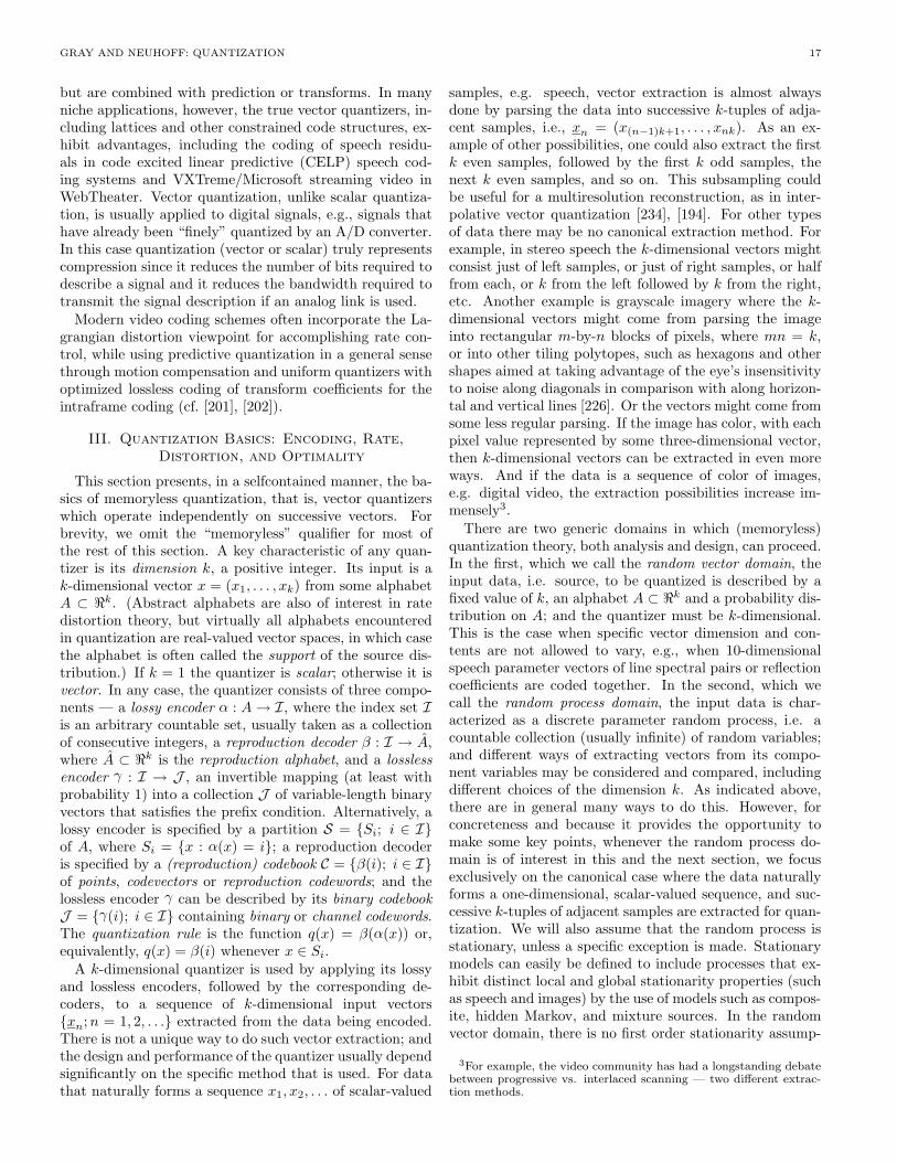
GRAY AND NEUHOFF: QUANTIZATION 17
but are combined with prediction or transforms. In manyniche applications, however, the true vector quantizers, in-cluding lattices and other constrained code structures, ex-hibit advantages, including the coding of speech residu-als in code excited linear predictive (CELP) speech cod-ing systems and VXTreme/Microsoft streaming video inWebTheater. Vector quantization, unlike scalar quantiza-tion, is usually applied to digital signals, e.g., signals thathave already been “finely” quantized by an A/D converter.In this case quantization (vector or scalar) truly representscompression since it reduces the number of bits required todescribe a signal and it reduces the bandwidth required totransmit the signal description if an analog link is used.
Modern video coding schemes often incorporate the La-grangian distortion viewpoint for accomplishing rate con-trol, while using predictive quantization in a general sensethrough motion compensation and uniform quantizers withoptimized lossless coding of transform coefficients for theintraframe coding (cf. [201], [202]).
III. Quantization Basics: Encoding, Rate,Distortion, and Optimality
This section presents, in a selfcontained manner, the ba-sics of memoryless quantization, that is, vector quantizerswhich operate independently on successive vectors. Forbrevity, we omit the “memoryless” qualifier for most ofthe rest of this section. A key characteristic of any quan-tizer is its dimension k, a positive integer. Its input is ak-dimensional vector x = (x1, . . . , xk) from some alphabetA ⊂ <k. (Abstract alphabets are also of interest in ratedistortion theory, but virtually all alphabets encounteredin quantization are real-valued vector spaces, in which casethe alphabet is often called the support of the source dis-tribution.) If k = 1 the quantizer is scalar; otherwise it isvector. In any case, the quantizer consists of three compo-nents — a lossy encoder α : A→ I, where the index set Iis an arbitrary countable set, usually taken as a collectionof consecutive integers, a reproduction decoder β : I → A,where A ⊂ <k is the reproduction alphabet, and a losslessencoder γ : I → J , an invertible mapping (at least withprobability 1) into a collection J of variable-length binaryvectors that satisfies the prefix condition. Alternatively, alossy encoder is specified by a partition S = {Si; i ∈ I}of A, where Si = {x : α(x) = i}; a reproduction decoderis specified by a (reproduction) codebook C = {β(i); i ∈ I}of points, codevectors or reproduction codewords; and thelossless encoder γ can be described by its binary codebookJ = {γ(i); i ∈ I} containing binary or channel codewords.The quantization rule is the function q(x) = β(α(x)) or,equivalently, q(x) = β(i) whenever x ∈ Si.
A k-dimensional quantizer is used by applying its lossyand lossless encoders, followed by the corresponding de-coders, to a sequence of k-dimensional input vectors{xn;n = 1, 2, . . .} extracted from the data being encoded.There is not a unique way to do such vector extraction; andthe design and performance of the quantizer usually dependsignificantly on the specific method that is used. For datathat naturally forms a sequence x1, x2, . . . of scalar-valued
samples, e.g. speech, vector extraction is almost alwaysdone by parsing the data into successive k-tuples of adja-cent samples, i.e., xn = (x(n−1)k+1, . . . , xnk). As an ex-ample of other possibilities, one could also extract the firstk even samples, followed by the first k odd samples, thenext k even samples, and so on. This subsampling couldbe useful for a multiresolution reconstruction, as in inter-polative vector quantization [234], [194]. For other typesof data there may be no canonical extraction method. Forexample, in stereo speech the k-dimensional vectors mightconsist just of left samples, or just of right samples, or halffrom each, or k from the left followed by k from the right,etc. Another example is grayscale imagery where the k-dimensional vectors might come from parsing the imageinto rectangular m-by-n blocks of pixels, where mn = k,or into other tiling polytopes, such as hexagons and othershapes aimed at taking advantage of the eye’s insensitivityto noise along diagonals in comparison with along horizon-tal and vertical lines [226]. Or the vectors might come fromsome less regular parsing. If the image has color, with eachpixel value represented by some three-dimensional vector,then k-dimensional vectors can be extracted in even moreways. And if the data is a sequence of color of images,e.g. digital video, the extraction possibilities increase im-mensely3.
There are two generic domains in which (memoryless)quantization theory, both analysis and design, can proceed.In the first, which we call the random vector domain, theinput data, i.e. source, to be quantized is described by afixed value of k, an alphabet A ⊂ <k and a probability dis-tribution on A; and the quantizer must be k-dimensional.This is the case when specific vector dimension and con-tents are not allowed to vary, e.g., when 10-dimensionalspeech parameter vectors of line spectral pairs or reflectioncoefficients are coded together. In the second, which wecall the random process domain, the input data is char-acterized as a discrete parameter random process, i.e. acountable collection (usually infinite) of random variables;and different ways of extracting vectors from its compo-nent variables may be considered and compared, includingdifferent choices of the dimension k. As indicated above,there are in general many ways to do this. However, forconcreteness and because it provides the opportunity tomake some key points, whenever the random process do-main is of interest in this and the next section, we focusexclusively on the canonical case where the data naturallyforms a one-dimensional, scalar-valued sequence, and suc-cessive k-tuples of adjacent samples are extracted for quan-tization. We will also assume that the random process isstationary, unless a specific exception is made. Stationarymodels can easily be defined to include processes that ex-hibit distinct local and global stationarity properties (suchas speech and images) by the use of models such as compos-ite, hidden Markov, and mixture sources. In the randomvector domain, there is no first order stationarity assump-
3For example, the video community has had a longstanding debatebetween progressive vs. interlaced scanning — two different extrac-tion methods.
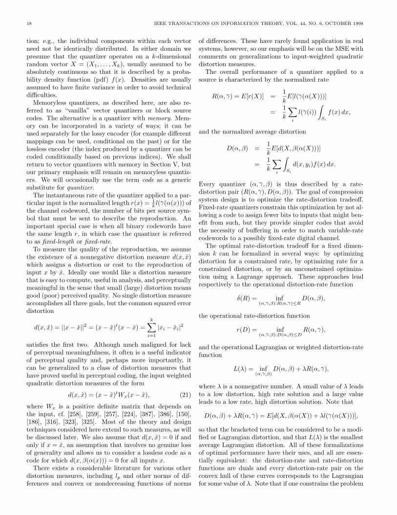
18 IEEE TRANSACTIONS ON INFORMATION THEORY, VOL. 44, NO. 6, OCTOBER 1998
tion; e.g., the individual components within each vectorneed not be identically distributed. In either domain wepresume that the quantizer operates on a k-dimensionalrandom vector X = (X1, . . . , Xk), usually assumed to beabsolutely continuous so that it is described by a proba-bility density function (pdf) f(x). Densities are usuallyassumed to have finite variance in order to avoid technicaldifficulties.
Memoryless quantizers, as described here, are also re-ferred to as “vanilla” vector quantizers or block sourcecodes. The alternative is a quantizer with memory. Mem-ory can be incorporated in a variety of ways; it can beused separately for the lossy encoder (for example differentmappings can be used, conditional on the past) or for thelossless encoder (the index produced by a quantizer can becoded conditionally based on previous indices). We shallreturn to vector quantizers with memory in Section V, butour primary emphasis will remain on memoryless quantiz-ers. We will occasionally use the term code as a genericsubstitute for quantizer.
The instantaneous rate of the quantizer applied to a par-ticular input is the normalized length r(x) = 1
k l(γ(α(x))) ofthe channel codeword, the number of bits per source sym-bol that must be sent to describe the reproduction. Animportant special case is when all binary codewords havethe same length r, in which case the quantizer is referredto as fixed-length or fixed-rate.
To measure the quality of the reproduction, we assumethe existence of a nonnegative distortion measure d(x, x)which assigns a distortion or cost to the reproduction ofinput x by x. Ideally one would like a distortion measurethat is easy to compute, useful in analysis, and perceptuallymeaningful in the sense that small (large) distortion meansgood (poor) perceived quality. No single distortion measureaccomplishes all three goals, but the common squared errordistortion
d(x, x) = ||x− x||2 = (x− x)t(x− x) =k∑i=1
|xi − xi|2
satisfies the first two. Although much maligned for lackof perceptual meaningfulness, it often is a useful indicatorof perceptual quality and, perhaps more importantly, itcan be generalized to a class of distortion measures thathave proved useful in perceptual coding, the input weightedquadratic distortion measures of the form
d(x, x) = (x− x)tWx(x− x), (21)
where Wx is a positive definite matrix that depends onthe input, cf. [258], [259], [257], [224], [387], [386], [150],[186], [316], [323], [325]. Most of the theory and designtechniques considered here extend to such measures, as willbe discussed later. We also assume that d(x, x) = 0 if andonly if x = x, an assumption that involves no genuine lossof generality and allows us to consider a lossless code as acode for which d(x, β(α(x))) = 0 for all inputs x.
There exists a considerable literature for various otherdistortion measures, including lp and other norms of dif-ferences and convex or nondecreasing functions of norms
of differences. These have rarely found application in realsystems, however, so our emphasis will be on the MSE withcomments on generalizations to input-weighted quadraticdistortion measures.
The overall performance of a quantizer applied to asource is characterized by the normalized rate
R(α, γ) = E[r(X)] =1kE[l(γ(α(X)))]
=1k
∑i
l(γ(i))∫Si
f(x) dx,
and the normalized average distortion
D(α, β) =1kE[d(X,β(α(X)))]
=1k
∑i
∫Si
d(x, yi)f(x) dx.
Every quantizer (α, γ, β) is thus described by a rate-distortion pair (R(α, γ), D(α, β)). The goal of compressionsystem design is to optimize the rate-distortion tradeoff.Fixed-rate quantizers constrain this optimization by not al-lowing a code to assign fewer bits to inputs that might ben-efit from such, but they provide simpler codes that avoidthe necessity of buffering in order to match variable-ratecodewords to a possibly fixed-rate digital channel.
The optimal rate-distortion tradeoff for a fixed dimen-sion k can be formalized in several ways: by optimizingdistortion for a constrained rate, by optimizing rate for aconstrained distortion, or by an unconstrained optimiza-tion using a Lagrange approach. These approaches leadrespectively to the operational distortion-rate function
δ(R) = inf(α,γ,β):R(α,γ)≤R
D(α, β),
the operational rate-distortion function
r(D) = inf(α,γ,β):D(α,β)≤D
R(α, γ),
and the operational Lagrangian or weighted distortion-ratefunction
L(λ) = inf(α,γ,β)
D(α, β) + λR(α, γ),
where λ is a nonnegative number. A small value of λ leadsto a low distortion, high rate solution and a large valueleads to a low rate, high distortion solution. Note that
D(α, β) + λR(α, γ) = E[d(X,β(α(X)) + λl(γ(α(X)))],
so that the bracketed term can be considered to be a modi-fied or Lagrangian distortion, and that L(λ) is the smallestaverage Lagrangian distortion. All of these formalizationsof optimal performance have their uses, and all are essen-tially equivalent: the distortion-rate and rate-distortionfunctions are duals and every distortion-rate pair on theconvex hull of these curves corresponds to the Lagrangianfor some value of λ. Note that if one constrains the problem
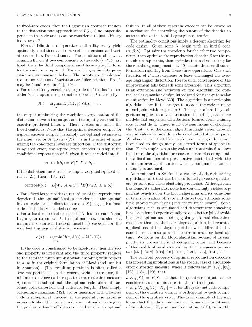
GRAY AND NEUHOFF: QUANTIZATION 19
to fixed-rate codes, then the Lagrangian approach reducesto the distortion rate approach since R(α, γ) no longer de-pends on the code and γ can be considered as just a binaryindexing of I.
Formal definitions of quantizer optimality easily yieldoptimality conditions as direct vector extensions and vari-ations on Lloyd’s conditions. The conditions all have acommon flavor: if two components of the code (α, γ, β) arefixed, then the third component must have a specific formfor the code to be optimal. The resulting optimality prop-erties are summarized below. The proofs are simple andrequire no calculus of variations or differentiation. Proofsmay be found, e.g., in [94], [196].• For a fixed lossy encoder α, regardless of the lossless en-coder γ, the optimal reproduction decoder β is given by
β(i) = argminy
E[d(X, y)|α(X) = i],
the output minimizing the conditional expectation of thedistortion between the output and the input given that theencoder produced index i. These vectors are called theLloyd centroids. Note that the optimal decoder output fora given encoder output i is simply the optimal estimate ofthe input vector X given α(X) = i in the sense of mini-mizing the conditional average distortion. If the distortionis squared error, the reproduction decoder is simply theconditional expectation of X given it was encoded into i:
centroid(Si) = E[X|X ∈ Si].
If the distortion measure is the input-weighted squared er-ror of (21), then [318], [224]
centroid(Si) = E[WX |X ∈ Si]−1E[WXX|X ∈ Si].
• For a fixed lossy encoder α, regardless of the reproductiondecoder β, the optimal lossless encoder γ is the optimallossless code for the discrete source α(X), e.g., a Huffmancode for the lossy encoded source.• For a fixed reproduction decoder β, lossless code γ andLagrangian parameter λ, the optimal lossy encoder is aminimum distortion (nearest neighbor) encoder for themodified Lagrangian distortion measure:
α(x) = argmini∈I
(d(x, β(i)) + λl(γ(i))).
If the code is constrained to be fixed-rate, then the sec-ond property is irrelevant and the third property reducesto the familiar minimum distortion encoding with respectto d, as in the original formulation of Lloyd (and implicitin Shannon). (The resulting partition is often called aVoronoi partition.) In the general variable-rate case, theminimum distance (with respect to the distortion measured) encoder is suboptimal; the optimal rule takes into ac-count both distortion and codeword length. Thus simplycascading a minimum MSE vector quantizer with a losslesscode is suboptimal. Instead, in the general case instanta-neous rate should be considered in an optimal encoding, asthe goal is to trade off distortion and rate in an optimal
fashion. In all of these cases the encoder can be viewed asa mechanism for controlling the output of the decoder soas to minimize the total Lagrangian distortion.
The optimality conditions imply a descent algorithm forcode design: Given some λ, begin with an initial code(α, β, γ). Optimize the encoder α for the other two compo-nents, then optimize the reproduction decoder β for the re-maining components, then optimize the lossless coder γ forthe remaining components. Let T denote the overall trans-formation resulting from these three operations. One suchiteration of T must decrease or leave unchanged the aver-age Lagrangian distortion. Iterate until convergence or theimprovement falls beneath some threshold. This algorithmis an extension and variation on the algorithm for opti-mal scalar quantizer design introduced for fixed-rate scalarquantization by Lloyd[330]. The algorithm is a fixed-pointalgorithm since if it converges to a code, the code must bea fixed point with respect to T . This generalized Lloyd al-gorithm applies to any distribution, including parametricmodels and empirical distributions formed from trainingsets of real data. There is no obvious means of choosingthe “best” λ, so the design algorithm might sweep throughseveral values to provide a choice of rate-distortion pairs.We also mention that Lloyd style iterative algorithms havebeen used to design many structured forms of quantiza-tion. For example, when the codes are constrained to havefixed rate, the algorithm becomes k-means clustering, find-ing a fixed number of representative points that yield theminimum average distortion when a minimum distortionmapping is assumed.
As mentioned in Section I, a variety of other clusteringalgorithms exist that can be used to design vector quantiz-ers (or solve any other clustering problems). Although eachhas found its adherents, none has convincingly yielded sig-nificant benefits over the Lloyd algorithm and its variationsin terms of trading off rate and distortion, although somehave proved much faster (and others much slower). Somealgorithms such as simulated and deterministic annealinghave been found experimentally to do a better job of avoid-ing local optima and finding globally optimal distortion-rate pairs than has the basic Lloyd algorithm, but repeatedapplications of the Lloyd algorithm with different initialconditions has also proved effective in avoiding local op-tima. We focus on the Lloyd algorithm because of its sim-plicity, its proven merit at designing codes, and becauseof the wealth of results regarding its convergence proper-ties [451], [418], [108], [91], [101], [321], [335], [131], [36].
The centroid property of optimal reproduction decodershas interesting implications in the special case of a squared-error distortion measure, where it follows easily [137], [60],[193], [184], [196] that• E[q(X)] = E[X], so that the quantizer output can beconsidered as an unbiased estimator of the input.• E[qi(X)(qj(X)−Xj)] = 0, for all i, j so that each compo-nent of the quantizer output is orthogonal to each compo-nent of the quantizer error. This is an example of the wellknown fact that the minimum mean squared error estimateof an unknown, X, given an observation, α(X), causes the
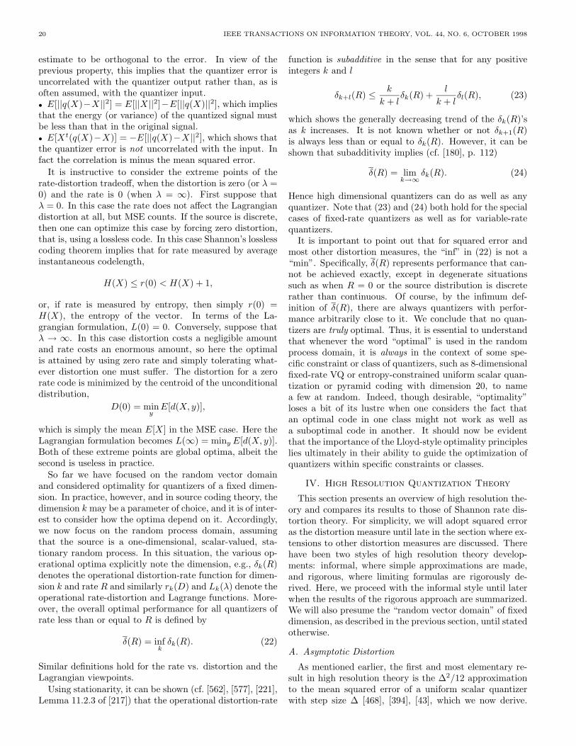
20 IEEE TRANSACTIONS ON INFORMATION THEORY, VOL. 44, NO. 6, OCTOBER 1998
estimate to be orthogonal to the error. In view of theprevious property, this implies that the quantizer error isuncorrelated with the quantizer output rather than, as isoften assumed, with the quantizer input.• E[||q(X)−X||2] = E[||X||2]−E[||q(X)||2], which impliesthat the energy (or variance) of the quantized signal mustbe less than that in the original signal.• E[Xt(q(X)−X)] = −E[||q(X)−X||2], which shows thatthe quantizer error is not uncorrelated with the input. Infact the correlation is minus the mean squared error.
It is instructive to consider the extreme points of therate-distortion tradeoff, when the distortion is zero (or λ =0) and the rate is 0 (when λ = ∞). First suppose thatλ = 0. In this case the rate does not affect the Lagrangiandistortion at all, but MSE counts. If the source is discrete,then one can optimize this case by forcing zero distortion,that is, using a lossless code. In this case Shannon’s losslesscoding theorem implies that for rate measured by averageinstantaneous codelength,
H(X) ≤ r(0) < H(X) + 1,
or, if rate is measured by entropy, then simply r(0) =H(X), the entropy of the vector. In terms of the La-grangian formulation, L(0) = 0. Conversely, suppose thatλ → ∞. In this case distortion costs a negligible amountand rate costs an enormous amount, so here the optimalis attained by using zero rate and simply tolerating what-ever distortion one must suffer. The distortion for a zerorate code is minimized by the centroid of the unconditionaldistribution,
D(0) = minyE[d(X, y)],
which is simply the mean E[X] in the MSE case. Here theLagrangian formulation becomes L(∞) = miny E[d(X, y)].Both of these extreme points are global optima, albeit thesecond is useless in practice.
So far we have focused on the random vector domainand considered optimality for quantizers of a fixed dimen-sion. In practice, however, and in source coding theory, thedimension k may be a parameter of choice, and it is of inter-est to consider how the optima depend on it. Accordingly,we now focus on the random process domain, assumingthat the source is a one-dimensional, scalar-valued, sta-tionary random process. In this situation, the various op-erational optima explicitly note the dimension, e.g., δk(R)denotes the operational distortion-rate function for dimen-sion k and rate R and similarly rk(D) and Lk(λ) denote theoperational rate-distortion and Lagrange functions. More-over, the overall optimal performance for all quantizers ofrate less than or equal to R is defined by
δ(R) = infkδk(R). (22)
Similar definitions hold for the rate vs. distortion and theLagrangian viewpoints.
Using stationarity, it can be shown (cf. [562], [577], [221],Lemma 11.2.3 of [217]) that the operational distortion-rate
function is subadditive in the sense that for any positiveintegers k and l
δk+l(R) ≤ k
k + lδk(R) +
l
k + lδl(R), (23)
which shows the generally decreasing trend of the δk(R)’sas k increases. It is not known whether or not δk+1(R)is always less than or equal to δk(R). However, it can beshown that subadditivity implies (cf. [180], p. 112)
δ(R) = limk→∞
δk(R). (24)
Hence high dimensional quantizers can do as well as anyquantizer. Note that (23) and (24) both hold for the specialcases of fixed-rate quantizers as well as for variable-ratequantizers.
It is important to point out that for squared error andmost other distortion measures, the “inf” in (22) is not a“min”. Specifically, δ(R) represents performance that can-not be achieved exactly, except in degenerate situationssuch as when R = 0 or the source distribution is discreterather than continuous. Of course, by the infimum def-inition of δ(R), there are always quantizers with perfor-mance arbitrarily close to it. We conclude that no quan-tizers are truly optimal. Thus, it is essential to understandthat whenever the word “optimal” is used in the randomprocess domain, it is always in the context of some spe-cific constraint or class of quantizers, such as 8-dimensionalfixed-rate VQ or entropy-constrained uniform scalar quan-tization or pyramid coding with dimension 20, to namea few at random. Indeed, though desirable, “optimality”loses a bit of its lustre when one considers the fact thatan optimal code in one class might not work as well asa suboptimal code in another. It should now be evidentthat the importance of the Lloyd-style optimality principleslies ultimately in their ability to guide the optimization ofquantizers within specific constraints or classes.
IV. High Resolution Quantization Theory
This section presents an overview of high resolution the-ory and compares its results to those of Shannon rate dis-tortion theory. For simplicity, we will adopt squared erroras the distortion measure until late in the section where ex-tensions to other distortion measures are discussed. Therehave been two styles of high resolution theory develop-ments: informal, where simple approximations are made,and rigorous, where limiting formulas are rigorously de-rived. Here, we proceed with the informal style until laterwhen the results of the rigorous approach are summarized.We will also presume the “random vector domain” of fixeddimension, as described in the previous section, until statedotherwise.
A. Asymptotic Distortion
As mentioned earlier, the first and most elementary re-sult in high resolution theory is the ∆2/12 approximationto the mean squared error of a uniform scalar quantizerwith step size ∆ [468], [394], [43], which we now derive.
GRAY AND NEUHOFF: QUANTIZATION 21
Consider an N -level uniform quantizer q whose levels arey1, . . . , yN , with yi = yi−1 + ∆. When this quantizer isapplied to a continuous random variable X with proba-bility density f(x), when ∆ is small, and when overloaddistortion can be ignored, the mean squared error (MSE)distortion may be approximated as follows:
D(q) = E[(X − q(X))2]
∼=N∑i=1
∫ yi+∆/2
yi−∆/2
(x− yi)2f(x) dx
∼=N∑i=1
f(yi)∫ yi+∆/2
yi−∆/2
(x− yi)2dx
=∆2
12
N∑i=1
f(yi)∆
∼= ∆2
12
∫ yN+∆/2
y1−∆/2
f(x) dx
∼= ∆2
12.
The first approximation in the above derives from ignoringoverload distortion. If the source density is entirely con-tained in the granular region of the quantizer, then thisapproximation is not needed. The second approximationderives from observing that the density may be approxi-mated as a constant on a small interval. Usually, as in themean value theorem of integration, one assumes the densityis continuous, but as any measurable function is approxi-mately continuous, when ∆ is sufficiently small this ap-proximation is valid even for discontinuous densities. Thethird approximation derives from recognizing that by thedefinition of a Riemann integral,
∑Ni=1 f(yi)∆ is approxi-
mately equal to the integral of f . Finally, the last approx-imation derives from again ignoring the overload region.As mentioned in earlier sections, there are situations, suchas variable-rate quantization where an infinite number oflevels are permitted. In such cases, if the support of theuniform scalar quantizer contains that of the source den-sity, then there will be no overload distortion to ignore, andagain we have D ∼= ∆2/12.
It is important to mention the sense in which D is ap-proximated by ∆2/12. After all, when ∆ is small, both Dand ∆2/12 will be small, so it is not saying much to assertthat their difference is small. Rather, as discussed later inthe context of the rigorous framework for high resolutiontheory, it can be shown that under ordinary conditions, theratio of D and ∆2/12 tends to 1 as ∆ decreases. Thoughwe will not generally mention it, all future high resolutionapproximations discussed in this paper will also hold in thisratio-tending-to-one sense.
Each of the assumptions and simple approximationsmade in deriving ∆2/12 reoccurs in some guise in thederivation of all subsequent high-resolution formulas, suchas for nonuniform, vector and variable-rate quantizers.Thus, they might be said to be principal suppositions. In-deed the small cell type of supposition is what gives thetheory its “high resolution” name.
In uniform quantization, all cells have the same size andshape and the levels are in the center of each cell (exceptfor the outermost cells which are ignored). Thus, the cellsize ∆ is the key performance determining gross charac-teristic. In more, advanced e.g. vector, quantization, cellsmay differ in size and shape, and the codevectors need notbe in the centers of the cells. Consequently, other grosscharacterizations are needed. These are the point densityand the inertial profile.
The point density of a vector quantizer is the direct ex-tension of the point density introduced in Section II. Thatis, it is a nonnegative, usually smooth function λ(x) that,when integrated over a region, determines the approximatefraction of codevectors contained in that region. In fixed-rate coding, the point density is usually normalized by thenumber of codevectors so that its total integral is one. Invariable-rate coding, where the number of codevectors isnot a key performance determining parameter and mayeven be infinite, the point density is usually left unnor-malized. As we consider fixed-rate coding first, we willpresume λ is normalized, until stated otherwise. Thereis clearly an inverse relationship between the point den-sity and the volume of cells, namely, λ(x) ∼= (Nvol(Sx))−1,where as before, N is the number of codevectors or cellsand Sx denotes the cell containing x.
As with any density that describes a discrete set ofpoints, there is not a unique way to define it for a specificquantizer. Rather the point density is intended as a highlevel, gross characterization, or a model or target to whicha quantizer aspires. It describes the codevectors, in muchthe way that a probability density describes a set of datapoints — it does not say exactly where they are located,but roughly characterizes their distribution. Quantizerswith different numbers of codevectors can be compared onthe basis of their point density, and there is an ideal pointdensity to which quantizers aspire — they cannot achieveit exactly, but may approximate it. Nevertheless, there aretimes when a concrete definition of the point density of aspecific quantizer is needed. In such cases, the followingis often used: the specific point density of a quantizer q isλq(x) ≡ (Nvol(Sx))−1. This piecewise constant functioncaptures all the (fine) detail in the quantizer’s partition, incontrast to the usual notion of a point density as a grosscharacterization. As an example of its use, we mention thatfor fixed-rate quantization, the ideal point density λ(x) isusually a smooth function, closely related to the sourcedensity, and one may say that a quantizer has point den-sity approximately λ(x) if λq(x) ∼= λ(x) for all x in someset with high probability (relative to the source density).When a scalar quantizer is implemented as a compander,λ(x) is proportional to the derivative of the compressorfunction applied to the input. Though the notion of pointdensity would no doubt have been recognizable to the earli-est contributors such as Bennett, Panter and Dite, as men-tioned earlier, it was not explicitly introduced until Lloyd’swork [330].
In nonuniform scalar quantization and vector quantiza-tion, there is the additional issue of codevector placement
22 IEEE TRANSACTIONS ON INFORMATION THEORY, VOL. 44, NO. 6, OCTOBER 1998
within cells and, in the latter case, of cell shape. The effectof point placement and cell shape is exhibited in the fol-lowing approximation to the contribution of a small cell Siwith codevector yi to the MSE of a k-dimensional vectorquantizer:
Di(q) =1k
∫Si
||x− yi||2f(x) dx (25)
∼= f(yi)M(Si, yi)vol(Si)1+2/k, (26)
where M(Si, yi) is the normalized moment of inertia of thecell Si about the point yi, defined by
M(Si, yi) ≡1k
1vol(Si)1+2/k
∫Si
||x− yi||2 dx.
Normalizing by volume makes M independent of the sizeof the cell. Normalizing by dimension yields a kind of in-variance to dimension, namely that M(Si × Si, (yi, yi)) =M(Si, yi). We often write M(Si) when yi is clear from thecontext. The normalized moment of inertia, and the result-ing contribution Di(q), is smaller for sphere-like cells withcodevectors in the center than for cells that are oblong,have sharply pointed vertices, or have displaced codevec-tors. In the latter cases, there are more points farther fromyi that contribute substantially to normalized moment ofinertia, especially when dimension is large.
In some quantizers, such as uniform scalar and latticequantizers, all cells (with the exception of the outermostcells) have the same shape and the same placement ofcodevectors within cells. In other quantizers, however, cellshape or codevector placement varies with position. Insuch cases, it is useful to characterize the variation of cellnormalized moment of inertia by a nonnegative, usuallysmooth function m(x), called the inertial profile. Thatis, m(x) ∼= M(Si, yi) when x ∈ Si. As with point den-sities, we do not define m(x) to be equal to M(Sx, q(x)),because we want it to be a high level gross characteriza-tion or model to which a quantizer aspires. Instead we letmq(x) ≡ M(Sx, q(x)) be called the specific inertial profileof the quantizer q. This is a piecewise constant functionthat captures the fine details of cell normalized moment ofinertia.
Returning to Di(q) expressed in (26), the effect of cellsize is obviously in the term vol(Si). Using the inverserelationship between point density and cell volume yields
Di(q) ∼=1N
2k
f(yi)M(Si, yi)λ
2k (yi)
vol(Si)
which shows how point density locally influences distor-tion. Summing the above over all cells and recognizing thesum as an approximation to an integral yields the followingapproximation to the distortion of a vector quantizer
D(q) ∼= 1N
2k
∫m(x)λ
2k (x)
f(x) dx. (27)
For scalar quantizers (k = 1) with points in the middle ofthe cells, m(x) = 1
12 and the above reduces to
D(q) ∼= 112
1N2
∫1
λ2(x)f(x) dx (28)
which is what Bennett [43] found for companders, as re-stated in terms of point densities by Lloyd [330]. Both (28)and the more general formula (27) are called Bennett’s in-tegral. The extension of Bennett’s integral to vector quan-tizers was first made by Gersho (1979) [193] for quantizerswith congruent cells for which the concept of inertial profilewas not needed, and then to vector quantizers with varyingcell shapes (and codevector placements) by Na and Neuhoff(1995) [365].
Bennett’s integral (27) can be expected to be a good ap-proximation under the following conditions: (i) Most cellsare small enough that f(x) can be approximated as beingconstant over the cell. (There can be some large cells wheref(x) is very small.) Ordinarily, this requires N to be large.(ii) The specific point density of the quantizer approxi-mately equals λ(x) on a high probability set of x’s. (iii)The specific inertial profile approximately equals m(x) ona high probability set of x’s. (iv) Adjacent cells have sim-ilar volumes. The last condition rules out quantizers suchas a scalar one whose cells have alternating lengths such as∆, 1
2∆, 12∆,∆, 1
2∆, 12∆,∆, . . . . The point density of such
a quantizer is λ(x) = 32∆N , because there are 3 points in
an interval of width 2∆. Assuming, for simplicity, that thesource density is uniform on [0,1], it is easy to computeD = 5
96∆2, whereas Bennett’s integral equals 127∆2. One
may obtain the correct distortion by separately applyingBennett’s integral to the union of intervals of length ∆ andto the union of intervals of length 1
2∆. The problem is thatBennett’s integral is not linear in the point density. So forit to be accurate, cell size must change slowly or only oc-casionally. Since Bennett’s integral is linear in the inertialprofile, it is not necessary to assume that adjacent cellshave similar shapes, although one would normally expectthis to be the case in situations where Bennett’s integralis applied. Examples of the use of the vector extension ofBennett’s integral will be given later.
Approximating the source density as a constant over eachquantization cell, which is a key step in the derivations of(26) and (28), is like assuming that the effect of quantiza-tion is to add noise that is uniformly distributed. However,the range of noise values must match the size and shape ofthe cell. And so when the cells are not all of the same sizeand shape, such quantization noise is obviously correlatedwith the vector X being quantized. On the other hand, foruniform scalar and lattice vector quantizers, the error andX are approximately uncorrelated. A more general result,mentioned in Section III, is that the correlation between theinput and the quantization error is approximately equal tothe MSE of the quantizer when the codevectors are approx-imately centroids.
B. Performance of the Best k-Dimensional, Fixed-RateQuantizers
Having Bennett’s integral for distortion, one can hopeto find a formula for δk(R), the operational distortion-ratefunction for k-dimensional, fixed-rate vector quantization,by choosing the key characteristics, point density and in-ertial profile, to minimize (27). Unfortunately, it is not
GRAY AND NEUHOFF: QUANTIZATION 23
known how to find the best inertial profile. Indeed, itis not even known what functions are allowable as iner-tial profiles. However, Gersho (1979) [193] made the nowwidely accepted conjecture that when rate is large, mostcells of a k-dimensional quantizer with rate R and mini-mum or nearly minimum MSE are approximately congru-ent to some basic tessellating4 k-dimensional cell shape Tk.In this case, the optimum inertial profile is a constant andBennett’s integral can be minimized by variational tech-niques or Holder’s inequality [222], [193], resulting in theoptimal point density
λ∗k(x) =f
kk+2 (x)∫
fkk+2 (x′) dx′
(29)
and the following approximation to the operationaldistortion-rate function: for large R
δk(R) ∼= Mkβkσ22−2R ≡ Zk(R), (30)
where Mk ≡M(Tk), which is the least normalized momentof inertia of k-dimensional tessellating polytopes, and
βk ≡1σ2
(∫f
kk+2 (x) dx
) k+2k
is the term depending on the source distribution. Divid-ing by variance makes βk invariant to a scaling of thesource. We will refer to Mk, βk and Zk(R) as, respec-tively, Gersho’s constant (in dimension k), Zador’s factor(for k-dimensional, fixed-rate quantization) and the Zador-Gersho function (for k-dimensional, fixed-rate quantiza-tion). (Zador’s role will be described later.) When k = 1,Z1(R) reduces to the Panter-Dite formula (8).
¿From the form of λ∗k(x) one may straightforwardly de-duce that cells are smaller and have higher probabilitywhere f(x) is larger, and that all cells contribute roughlythe same to the distortion; i.e. Di(q) in (26) is approxi-mately the same for all i, which is the “partial distortiontheorem” first deduced for scalar quantization by Panterand Dite.
A number of properties of Mk and βk are known; here,we mention just a few. Gersho’s constant Mk is known onlyfor k = 1 and 2, where Tk is, respectively, an interval anda regular hexagon. It is not known whether the Mk’s aremonotonically nonincreasing for all k, but it can be shownthat they form a subadditive sequence, which is a propertystrong enough to imply that the infimum over k equals thelimit as k tends to infinity. Though it has long been pre-sumed, only recently has it been directly shown that theMk’s tend to 1
2πe as k increases (Zamir and Feder [564]),which is the limit of the normalized moment of inertia ofk-dimensional spheres as k tends to infinity. Previously,
4A cell T “tessellates” if there exists a partition of <k whose cellsare, entirely, translations and rotations of T . The Voronoi cell of anylattice tessellates, but not all tessellations are generated by lattices.Gersho also conjectured that Tk would be admissible in the sensethat the Voronoi partition for the centroids of the tessellation wouldcoincide with the tessellation. But this is not essential.
the assertion that the Mk’s tend to 12πe depended on Ger-
sho’s conjecture. Zador’s factor βk tends to be smallerfor source densities that are more “compact” (lighter tailsand more uniform) and have more dependence among thesource variables.
Fortunately, high resolution theory need not rely solelyon Gersho’s conjecture, because Zador’s dissertation [561]and subsequent memo [562] showed that for large rate δ(R)has the form bkβkσ
22−2R, where bk is independent of thesource distribution. Thus Gersho’s conjecture is really justa conjecture about bk.
In deriving the key result, Zador first showed that fora random vector that is uniformly distributed on the unitcube, δ(R) has the form bk2−2R when R is large, whicheffectively defines bk. (In this case, βkσ2 = 1.) He thenused this to prove the general result by showing that noquantizer with high rate could do better than one whosepartition is hierarchically constructed by partitioning <kinto small equally sized cubes and then subdividing eachwith the partition of the quantizer that is best for a uniformdistribution on that cube, where the number of cells withineach cube depends on the source density in that cube. Inother words, the local structure of an asymptotically opti-mal quantizer can be that of the optimum quantizer for auniform distribution.
In this light, Gersho’s conjecture is true if and only if athigh rates one may obtain an asymptotically optimal quan-tizer for a uniform distribution by tessellating with Tk. Thelatter statement has been proven for k = 1 (cf. [106], p. 59)and for k = 2 by Fejes Toth (1959) [159]; see also [385]. Fork = 3, it is known that the best lattice tessellation is thebody-centered cubic lattice, which is generated by a trun-cated octahedron [35]. It has not been proven that this isthe best tessellation, though one would suspect that it is.In summary, Gersho’s conjecture is known to be true onlyfor k = 1 and 2. Might it be false for k ≥ 3? If it is,it might be that the best quantizers for a uniform sourcehave a periodic tessellation in which two or more cell shapesalternate in a periodic fashion, like the hexagons and pen-tagons on the surface of a soccer ball. If the cells in oneperiod of the tessellation have the same volumes, then onemay apply Bennett’s integral, and (30) holds with Mk re-placed by the average of the normalized moment of iner-tia of the cells in one period. However, if the cells haveunequal volumes, then as in the example given while dis-cussing Condition (iv) of Bennett’s integral, the MSE willbe the average of distortions computed by using Bennett’sintegral separately on the union of cells of each type, and amacrolevel definition of Mk will be needed. It might also bethat the structure of optimal quantizers is aperiodic. How-ever, it seems likely to us that, asymptotically, one couldalways find a quantizer with a periodic structure that isessentially as good as any aperiodic one.
It is an open question in dimensions three and abovewhether the best tessellation is a lattice. In most dimen-sions the best known tessellation is a lattice. However,tessellations that are better than the best known latticeshave recently been found for dimensions seven and nine by
24 IEEE TRANSACTIONS ON INFORMATION THEORY, VOL. 44, NO. 6, OCTOBER 1998
Agrell and Eriksson [149].¿From now on, we shall proceed assuming Gersho’s con-
jecture is correct, with the knowledge that if this is not thecase, then analyses based on Mk will be wrong (for k ≥ 3)by the factor Mk/bk, which will be larger than 1 (but prob-ably not much larger), and which in any case will convergeto one as k →∞, as discussed later.
C. Performance of the Best k-Dimensional, Variable-RateQuantizers
Extensions of high resolution theory to variable-ratequantization can also be based on Bennett’s integral,as well as approximations, originally due to Gish andPierce [204], to the entropy of the output of a quan-tizer. Two such approximations, which can be derivedusing approximations much like those used to derive Ben-nett’s integral, were stated earlier for scalar quantizers in(11) and (13). However, the approximation (13), whichsays that for quantizers with mostly small cells H(q) ∼=h(X) +E[log Λ(X)], where Λ(x) is the unnormalized pointdensity, holds equally well for vector quantizers, when Xis interpreted as a vector rather than a scalar variable. Asmentioned before, unnormalized point density is used be-cause with variable-rate quantization, the number of code-vectors is not a primary characteristic and may even beinfinite. For example, one can always add levels in a waythat has negligible impact on the distortion and entropy.
We could now proceed to use Bennett’s integral and theentropy approximation to find the operational distortion-rate function for variable-rate, k-dimensional, memorylessVQ. However, we wish to consider a somewhat more gen-eral case. Just as Gish and Pierce found something quiteinteresting by examining the best possible performance ofscalar quantization with block entropy coding, we will nowconsider the operational distortion-rate function for vectorquantization with block entropy coding. Specifically, weseek δk,L(R), which is defined to be the infimum of the dis-tortions of any quantizer with rate R or less, whose lossyencoder is k-dimensional and memoryless, and whose loss-less encoder simultaneously codes a block of L successivequantization indices with a variable-length prefix code. Ineffect, the overall code is a kL-dimensional, memorylessVQ. However, we will refer to it as a k-dimensional (mem-oryless) quantizer with L-th order variable-length coding(or L-th order entropy coding). When L = 1, the codebecomes a conventional memoryless, variable-rate vectorquantizer. It is convenient to let L = 0 connote fixed-length coding, so that δk,0(R) means the same as δk(R) ofthe previous section. By finding high resolution approxi-mations to δk,L(R) for all values of k ≥ 1 and L ≥ 0, wewill be able to compare the advantages of increasing the di-mension k of the quantizer to those of increasing the orderL of the entropy coder.
To find δk,L(R) we assume that the source produces asequence (X1, . . . , XL) of identical, but not necessarily in-dependent, k-dimensional random vectors, each with den-sity f(x). A straightforward generalization of (13) shows
that under high resolution conditions, the rate is given by
R ∼= 1kL
h(X1, . . . , XkL) +1k
∫f(x) log Λ(x) dx. (31)
On the other hand, the distortion of such a code may beapproximated using Bennett’s integral (27), with Λ(x)/N
2k
substituted for the normalized point density λ(x). Then, aswith fixed-rate vector quantization, one would like to findδk,L(R) by choosing the inertial profile m and the pointdensity Λ to minimize Bennett’s integral subject to a con-straint on the rate that the right-hand side of (31) be atmost R.
Once again, though it is not known how to find the bestinertial profile, Gersho’s conjecture suggests that when rateis large, the cells of the best rate-constrained quantizersare, mostly, congruent to Tk. Hence, from now on we shallassume that the inertial profile of the best variable-ratequantizers is, approximately, m(x) = Mk. In this case,using variational techniques or simply Jensen’s inequality,one can show that the best point density is uniform on allof <k (or at least over the support of the source density).In other words, all quantizer cells have the same size, asin a tessellation. Using this fact along with (27) and (31)yields
δk,L(R) ∼= MkγkLσ22−2R ≡ Zk,L(R), (32)
whereγk ≡
1σ2
22 1kh(X1,...,Xk)
is the term depending on the source distribution. Dividingby variance makes it invariant to scale. We call γk the (k-thorder) Zador entropy factor and Zk,L(R) a Zador-Gershofunction for variable-rate coding. Since fixed-rate codingis a special case of variable-length coding, it must be thatγk is less than or equal to βk in (30). This can be directlyverified using Jensen’s inequality [193].
In the case of scalar quantization (k = 1), the opti-mality of the uniform point density and the operationaldistortion-rate function δ1,L(R) were found by Gish andPierce (1968) [204]. Zador (1966) [562] considered the L =1 case and showed that δk,1(R) has the form ckγkσ
22−2R
when R is large, where ck is a constant that is indepen-dent of the source density and no larger than the constantbk that he found for fixed-rate quantization. Gersho [193]used the argument given above to find the form of δk,1(R)given in (32).
As with fixed-rate quantization, we shall proceed un-der the assumption that Gersho’s conjecture is correct, inwhich case ck = bk = Mk. If it is wrong, then our analy-ses will be off by the factor Mk/ck, which, as before, willprobably be just a little larger than one, and which in anycase will converge to one as k →∞.
D. Fixed-Rate Quantization with Arbitrary Dimension
We now restrict attention to the random process domainwherein the source is assumed to be a one-dimensional,scalar-valued, stationary random process. We seek a highresolution approximation to the operational distortion-rate
GRAY AND NEUHOFF: QUANTIZATION 25
function δ(R) ≡ infk δk(R), which represents the best pos-sible performance of any fixed-rate (memoryless) quan-tizer. As mentioned in Section III, for stationary sourcesδ(R) = limk→∞ δk(R). Therefore, taking the limit of thehigh resolution approximation (30) for δk(R) yields the factthat for large R
δ(R) ∼= M βσ22−2R ≡ Z(R), (33)
where
M = limk→∞
Mk =1
2πe,
β = limk→∞
βk,
andZ(R) ≡ lim
k→∞Zk(R)
is another Zador-Gersho function. This operationaldistortion-rate function was also derived by Zador [561],who showed that his unknown factors bk and ck convergedto 1
2πe . The derivation given here is due to Gersho [193].Notice that in this limiting case, there is no doubt aboutthe constant M .
As previously mentioned the Mk’s are subadditive, sothat they are smallest when k is large. Similarly, for sta-tionary sources it can be shown that the sequence {log βk}is also subadditive [193], so that they too are smallest whenk is large. Therefore another expression for the aboveZador-Gersho function is Z(R) = infk Zk(R).
E. The Benefits of Increasing Dimension in Fixed-RateQuantization
Continuing in the random process domain (stationarysources), the generally decreasing natures of Mk and βkdirectly quantify the benefits of increasing dimension infixed-rate quantization. (Of course, there is also a cost toincreasing dimension, namely, the increase in complexity.)For example, Mk decreases from 1
12 = .0833 for k = 1to the limit 1
2πe = .0586. In decibels, this represents a1.53 dB decrease in MSE. For an i.i.d. Gaussian source,βk decreases from 6
√3π = 32.6 for k = 1 to the limit
2πe = 17.1, which represents an additional 2.81 dB gain.In total, high dimensional quantization gains 4.35 dB overscalar quantization for the i.i.d. Gaussian source. For aGauss-Markov source with correlation coefficient ρ = .9,βk decreases from 6
√3π = 32.6 for k = 1 to the limit
2πe(1−ρ2) = 3.25 or a gain of 10.0 dB, yielding a total highdimensional VQ gain of 11.5 dB over scalar quantization.Because of the 6 dB per bit rule, any gain stated in dBcan be translated to a reduction in rate (bits/sample) bydividing by 6.02.
On the other hand, it is also important to understandwhat specific characteristics of vector quantizers improvewith dimension and by how much. Motivated by severalprior explanations [342], [333], [365], we offer the follow-ing. We wish to compare an optimal quantizer, qk, withdimension k to an optimal k′-dimensional quantizer, qk′with k′ >> k. To simplify the discussion, assume k′ is a
multiple of k. Though these two quantizers have differingdimensions, their characteristics can be fairly compared byby comparing qk′ to the “product” VQ qpr,k′ that is im-plicitly formed when qk is used k′/k times in succession.Specifically, the product quantizer has quantization rule
qpr,k′(x) = (qk(x1), . . . , qk(xk′/k)),
where x1, . . . , xk′/k are the successive k-tuples of x, andreproduction codebook Cpr,k′ consisting of the concatena-tions of all possible sequences of k′/k codevectors from qk’sreproduction codebook Ck. The subscripts “k” and “pr, k′”will be attached as needed to associate the appropriate fea-tures with the appropriate quantizer. The distortion andrate of the product quantizer are easily seen to be thoseof the k-dimensional VQ. Thus the shortcomings of an op-timal k-dimensional quantizer relative to an optimal highdimensional quantizer may be identified with those of theproduct quantizer — in particular, with the latter’s sub-optimal point density and inertial profile, which we nowfind.
To simplify discussion, assume for now that k = 1, andlet q1 be a fixed-rate scalar quantizer, with large rate, lev-els in the middle of the cells, and point density λsq(x1).The cells of the product quantizer qpr,k′ are k′-dimensionalrectangles formed by Cartesian products of cells from thescalar quantizer. When the scalar cells have the samewidth, a k′-dimensional cube is formed; otherwise a rect-angle is formed, i.e. an “oblong” cube. Since the widthsof the cells are, approximately, determined by λsq(x1), thepoint density and inertial profile of qpr,k′ are determinedby λsq. Specifically, from the rectangular nature of theproduct cells one obtains [365], [378]
λpr,k′(x) =k′∏i=1
λsq(xi) (34)
and
mpr,k′(x) =112
1k′∑k′
i=11
λ2sq(xi)(∏k′
i=11
λ2sq(xi)
) 1k′, (35)
which derive, respectively, from the facts that the volumeof a rectangle is the product of its side lengths, that thenormalized moment of inertia of a rectangle is that of acube (1/12) times the ratio of the arithmetic mean of thesquare of the side lengths to their geometric mean, and thatthe side lengths are determined by the scalar point den-sity. Note that along the diagonal of the first “quadrant”(where x1 = x2 = . . . = xk′), the product cells are cubesand mpr,k′(x) = 1/12, the minimum value. Off the diag-onal, the cells are usually rectangular and, consequently,mpr,k′(x) is larger.
To quantify the suboptimality of the product quantizer’sprincipal feature, we factor the ratio of the distortions ofqpr,k′(x) and qk′ , which is a kind of loss, into terms thatreflect the loss due to the inertial profile and point den-sity [365], [379]5
5Na and Neuhoff considered the ratio of the product code distortion
26 IEEE TRANSACTIONS ON INFORMATION THEORY, VOL. 44, NO. 6, OCTOBER 1998
L =D(qpr,k′)δk′(R)
∼= B(k′,mpr,k′ , λpr,k′ , f)B(k′,Mk′ , λ∗k′ , f)
=B(k′,mpr,k′ , λpr,k′ , f)B(k′,Mk′ , λpr,k′ , f)
× B(k′,Mk′ , λpr,k′ , f)B(k′,Mk′ , λ∗k′ , f)
= Lce × Lpt, (36)
where
B(k,m, λ, f) ≡∫
m(x)λ
2k (x)
f(x) dx
is the part of Bennett’s integral that does not depend onN , where the cell shape loss, Lce, is the ratio of the dis-tortion of the product quantizer to that of a hypotheticalquantizer with same point density and an optimal inertialprofile, and where the point density loss, Lpt, is the ratioof the distortion of a hypothetical quantizer with the pointdensity of the product quantizer and a constant (e.g. op-timal) inertial profile to that of a hypothetical quantizerwith an optimal point density and the same (constant) in-ertial profile. Substituting (35) into (36) and using the factthat for large k′, Mk′
∼= 12πe , one finds
L =πe
6×∫
1k′∑k′
i=11
λ2sq(xi)
fk′(x) dx∫1(∏k′
i=1λ2
sq(xi)
) 1k′fk′(x) dx
×
∫1∏k′
i=1λ
2k′sq (xi)
fk′(x) dx∫1
λ∗ 2k′
k′ (x)
fk′(x) dx
= Lsp × Lob × Lpt, (37)
where the cell shape loss has been factored into the productof a space filling loss [333]6, Lsp, which is the ratio of thenormalized moment of inertia of a cube to that of a highdimensional sphere, and an oblongitis loss, Lob, which isthe factor by which the rectangularity of the cells makesthe cell shape loss larger than the space filling loss.
To proceed further, consider first an i.i.d. source (sta-tionary and memoryless) and consider how to choose thescalar point density λsq(x1) in order to minimize L. On theone hand, choosing λsq(x1) to be uniform on the set wherethe one-dimensional density7 f1(x1) is not small causes theproduct cells in the region where the k′-dimensional densityfk′(x) is not small to be cubes and, consequently, makesLob∼= 1, which is the smallest possible value. However, it
causes the product point density to be poorly matched tothe source density and, as a result, Lpt is large. On theother hand, choosing λsq(x1) ∼= f1(x1) causes the product
to that of an optimal k-dimensional VQ for arbitrary k, not just forlarge k.
6Actually, Lookabaugh and Gray defined the inverse as a vectorquantizer advantage. The space-filling loss was called a cubic lossin [365]
7Dimension will be added as a subscript to f in places where thedimension of X needs to be emphasized.
quantizer to have, approximately, the optimal point den-sity8: λpr,k′(x) ∼=
∏k′
i=1 f1(xi) = fk′(x) ∼= λ∗k′(x), wherethe last step uses the fact that k′ is large. However, thischoice causes Lob to be infinite9. The best point density,as implicitly found by Panter and Dite, is the compromise
λ∗1(x1) =f
13
1 (x1)∫f
13
1 (u) du,
as given in (29). In the region where f1(x1) is not small,λ∗1(x1) is “more uniform” than λ1(x1) = f1(x1) that causesthe product quantizer to have the optimum point density.Therefore, it generates a product quantizer whose cells inthe region where fk′(x) is largest are more cubic, whichexplains why it has less oblongitis loss.
As an example, for an i.i.d. Gaussian source, the optimalchoice of scalar quantizer causes the product quantizer tohave 0.94 dB oblongitis loss and 1.88 dB point density loss.The sum of these, 2.81 dB, which equals 10 log10 β1/β, hasbeen called the “shape loss” [333] because it is determinedby the shape of the density — the more uniform the den-sity the less need for compromise because the scalar pointdensities leading to best product cell shapes and best pointdensity are more similar. Indeed, for a uniform source den-sity, there is no shape loss. In summary, for an i.i.d. source,in comparison to high dimensional quantization, the short-comings of scalar quantization with fixed-rate coding are:(1) the Lsp = 1.53 dB space filling loss and (2) the lack ofsufficient degrees of freedom to simultaneously attain goodinertial profile (small Lob) and good point density (smallLpt). On the other hand, it is often surprising to new-comers that vector quantization gains anything at all overscalar quantizers for i.i.d. sources, and secondly, that thegain is more than just the recovery of the space filling loss.
A similar comparison can be made between k-dimensional (k ≥ 2) and high dimensional VQ, by com-paring the product quantizer formed by k′/k uses of a k-dimensional VQ to an optimal k′-dimensional quantizer,for large k′. The results are that as k increases: (1) thespace filling loss Lsp = Mk/
12πe decreases, and (2) there
are more degrees of freedom so that less compromise isneeded between the k-dimensional point density that min-imizes oblongitis and the one that gives the optimal pointdensity. As a result the oblongitis, point density and shapelosses decrease to zero, along with the space filling loss.For the i.i.d. Gaussian source, these losses are plotted inFigure 5.
For sources with memory, scalar quantization (k = 1)engenders an additional loss due to its inability to exploitthe dependence between source samples. Specifically, whenthere is dependence/correlation between source samples,the product point density cannot match the ideal pointdensity, not even approximately. See [333], [365] for a defi-nition of memory loss. (One can factor both the point den-sity and oblongitis losses into two terms, one of which is
8The fact that product quantizers can have the optimal point den-sity is often overlooked.
9This implies that distortion will not decrease as 2−2R.
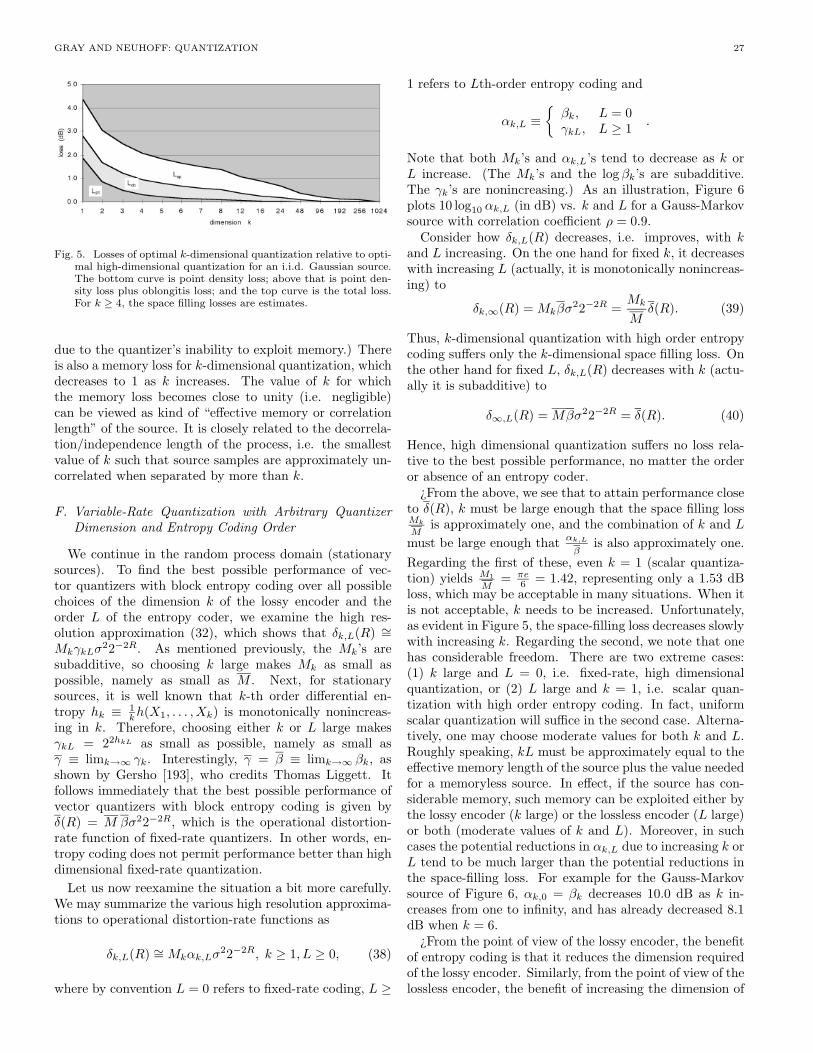
GRAY AND NEUHOFF: QUANTIZATION 27
Fig. 5. Losses of optimal k-dimensional quantization relative to opti-mal high-dimensional quantization for an i.i.d. Gaussian source.The bottom curve is point density loss; above that is point den-sity loss plus oblongitis loss; and the top curve is the total loss.For k ≥ 4, the space filling losses are estimates.
due to the quantizer’s inability to exploit memory.) Thereis also a memory loss for k-dimensional quantization, whichdecreases to 1 as k increases. The value of k for whichthe memory loss becomes close to unity (i.e. negligible)can be viewed as kind of “effective memory or correlationlength” of the source. It is closely related to the decorrela-tion/independence length of the process, i.e. the smallestvalue of k such that source samples are approximately un-correlated when separated by more than k.
F. Variable-Rate Quantization with Arbitrary QuantizerDimension and Entropy Coding Order
We continue in the random process domain (stationarysources). To find the best possible performance of vec-tor quantizers with block entropy coding over all possiblechoices of the dimension k of the lossy encoder and theorder L of the entropy coder, we examine the high res-olution approximation (32), which shows that δk,L(R) ∼=MkγkLσ
22−2R. As mentioned previously, the Mk’s aresubadditive, so choosing k large makes Mk as small aspossible, namely as small as M . Next, for stationarysources, it is well known that k-th order differential en-tropy hk ≡ 1
kh(X1, . . . , Xk) is monotonically nonincreas-ing in k. Therefore, choosing either k or L large makesγkL = 22hkL as small as possible, namely as small asγ ≡ limk→∞ γk. Interestingly, γ = β ≡ limk→∞ βk, asshown by Gersho [193], who credits Thomas Liggett. Itfollows immediately that the best possible performance ofvector quantizers with block entropy coding is given byδ(R) = M βσ22−2R, which is the operational distortion-rate function of fixed-rate quantizers. In other words, en-tropy coding does not permit performance better than highdimensional fixed-rate quantization.
Let us now reexamine the situation a bit more carefully.We may summarize the various high resolution approxima-tions to operational distortion-rate functions as
δk,L(R) ∼= Mkαk,Lσ22−2R, k ≥ 1, L ≥ 0, (38)
where by convention L = 0 refers to fixed-rate coding, L ≥
1 refers to Lth-order entropy coding and
αk,L ≡{βk, L = 0γkL, L ≥ 1 .
Note that both Mk’s and αk,L’s tend to decrease as k orL increase. (The Mk’s and the log βk’s are subadditive.The γk’s are nonincreasing.) As an illustration, Figure 6plots 10 log10 αk,L (in dB) vs. k and L for a Gauss-Markovsource with correlation coefficient ρ = 0.9.
Consider how δk,L(R) decreases, i.e. improves, with kand L increasing. On the one hand for fixed k, it decreaseswith increasing L (actually, it is monotonically nonincreas-ing) to
δk,∞(R) = Mkβσ22−2R =
Mk
Mδ(R). (39)
Thus, k-dimensional quantization with high order entropycoding suffers only the k-dimensional space filling loss. Onthe other hand for fixed L, δk,L(R) decreases with k (actu-ally it is subadditive) to
δ∞,L(R) = Mβσ22−2R = δ(R). (40)
Hence, high dimensional quantization suffers no loss rela-tive to the best possible performance, no matter the orderor absence of an entropy coder.
¿From the above, we see that to attain performance closeto δ(R), k must be large enough that the space filling lossMk
Mis approximately one, and the combination of k and L
must be large enough that αk,L
βis also approximately one.
Regarding the first of these, even k = 1 (scalar quantiza-tion) yields M1
M= πe
6 = 1.42, representing only a 1.53 dBloss, which may be acceptable in many situations. When itis not acceptable, k needs to be increased. Unfortunately,as evident in Figure 5, the space-filling loss decreases slowlywith increasing k. Regarding the second, we note that onehas considerable freedom. There are two extreme cases:(1) k large and L = 0, i.e. fixed-rate, high dimensionalquantization, or (2) L large and k = 1, i.e. scalar quan-tization with high order entropy coding. In fact, uniformscalar quantization will suffice in the second case. Alterna-tively, one may choose moderate values for both k and L.Roughly speaking, kL must be approximately equal to theeffective memory length of the source plus the value neededfor a memoryless source. In effect, if the source has con-siderable memory, such memory can be exploited either bythe lossy encoder (k large) or the lossless encoder (L large)or both (moderate values of k and L). Moreover, in suchcases the potential reductions in αk,L due to increasing k orL tend to be much larger than the potential reductions inthe space-filling loss. For example for the Gauss-Markovsource of Figure 6, αk,0 = βk decreases 10.0 dB as k in-creases from one to infinity, and has already decreased 8.1dB when k = 6.
¿From the point of view of the lossy encoder, the benefitof entropy coding is that it reduces the dimension requiredof the lossy encoder. Similarly, from the point of view of thelossless encoder, the benefit of increasing the dimension of
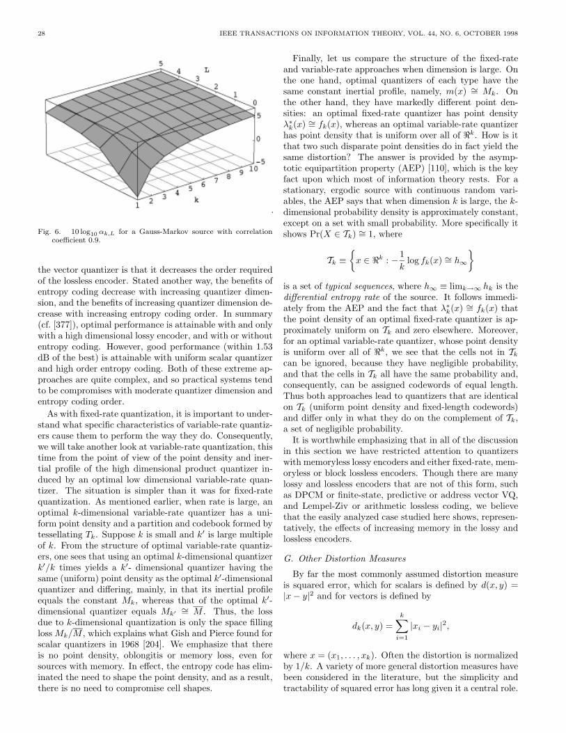
28 IEEE TRANSACTIONS ON INFORMATION THEORY, VOL. 44, NO. 6, OCTOBER 1998
.
Fig. 6. 10 log10 αk,L for a Gauss-Markov source with correlationcoefficient 0.9.
the vector quantizer is that it decreases the order requiredof the lossless encoder. Stated another way, the benefits ofentropy coding decrease with increasing quantizer dimen-sion, and the benefits of increasing quantizer dimension de-crease with increasing entropy coding order. In summary(cf. [377]), optimal performance is attainable with and onlywith a high dimensional lossy encoder, and with or withoutentropy coding. However, good performance (within 1.53dB of the best) is attainable with uniform scalar quantizerand high order entropy coding. Both of these extreme ap-proaches are quite complex, and so practical systems tendto be compromises with moderate quantizer dimension andentropy coding order.
As with fixed-rate quantization, it is important to under-stand what specific characteristics of variable-rate quantiz-ers cause them to perform the way they do. Consequently,we will take another look at variable-rate quantization, thistime from the point of view of the point density and iner-tial profile of the high dimensional product quantizer in-duced by an optimal low dimensional variable-rate quan-tizer. The situation is simpler than it was for fixed-ratequantization. As mentioned earlier, when rate is large, anoptimal k-dimensional variable-rate quantizer has a uni-form point density and a partition and codebook formed bytessellating Tk. Suppose k is small and k′ is large multipleof k. From the structure of optimal variable-rate quantiz-ers, one sees that using an optimal k-dimensional quantizerk′/k times yields a k′- dimensional quantizer having thesame (uniform) point density as the optimal k′-dimensionalquantizer and differing, mainly, in that its inertial profileequals the constant Mk, whereas that of the optimal k′-dimensional quantizer equals Mk′
∼= M . Thus, the lossdue to k-dimensional quantization is only the space fillingloss Mk/M , which explains what Gish and Pierce found forscalar quantizers in 1968 [204]. We emphasize that thereis no point density, oblongitis or memory loss, even forsources with memory. In effect, the entropy code has elim-inated the need to shape the point density, and as a result,there is no need to compromise cell shapes.
Finally, let us compare the structure of the fixed-rateand variable-rate approaches when dimension is large. Onthe one hand, optimal quantizers of each type have thesame constant inertial profile, namely, m(x) ∼= Mk. Onthe other hand, they have markedly different point den-sities: an optimal fixed-rate quantizer has point densityλ∗k(x) ∼= fk(x), whereas an optimal variable-rate quantizerhas point density that is uniform over all of <k. How is itthat two such disparate point densities do in fact yield thesame distortion? The answer is provided by the asymp-totic equipartition property (AEP) [110], which is the keyfact upon which most of information theory rests. For astationary, ergodic source with continuous random vari-ables, the AEP says that when dimension k is large, the k-dimensional probability density is approximately constant,except on a set with small probability. More specifically itshows Pr(X ∈ Tk) ∼= 1, where
Tk ≡{x ∈ <k : −1
klog fk(x) ∼= h∞
}is a set of typical sequences, where h∞ ≡ limk→∞ hk is thedifferential entropy rate of the source. It follows immedi-ately from the AEP and the fact that λ∗k(x) ∼= fk(x) thatthe point density of an optimal fixed-rate quantizer is ap-proximately uniform on Tk and zero elsewhere. Moreover,for an optimal variable-rate quantizer, whose point densityis uniform over all of <k, we see that the cells not in Tkcan be ignored, because they have negligible probability,and that the cells in Tk all have the same probability and,consequently, can be assigned codewords of equal length.Thus both approaches lead to quantizers that are identicalon Tk (uniform point density and fixed-length codewords)and differ only in what they do on the complement of Tk,a set of negligible probability.
It is worthwhile emphasizing that in all of the discussionin this section we have restricted attention to quantizerswith memoryless lossy encoders and either fixed-rate, mem-oryless or block lossless encoders. Though there are manylossy and lossless encoders that are not of this form, suchas DPCM or finite-state, predictive or address vector VQ,and Lempel-Ziv or arithmetic lossless coding, we believethat the easily analyzed case studied here shows, represen-tatively, the effects of increasing memory in the lossy andlossless encoders.
G. Other Distortion Measures
By far the most commonly assumed distortion measureis squared error, which for scalars is defined by d(x, y) =|x− y|2 and for vectors is defined by
dk(x, y) =k∑i=1
|xi − yi|2,
where x = (x1, . . . , xk). Often the distortion is normalizedby 1/k. A variety of more general distortion measures havebeen considered in the literature, but the simplicity andtractability of squared error has long given it a central role.
GRAY AND NEUHOFF: QUANTIZATION 29
Intuitively, the average squared error is the average energyor power in the quantization noise. The most common ex-tension of distortion measures for scalars is the rth powerdistortion, d(x, y) = |x− y|r. For example, Roe [443] gen-eralized Max’s formulation to distortion measures of thisform. Gish and Pierce [204] considered a more general dis-tortion measure of the form d(x, y) = L(x − y), where Lis a monotone increasing function of the magnitude of itsargument and L(0) = 0 with the added property that
M(v) ≡ 1v
∫ v/2
−v/2L(u) du
has the property that vM ′(v) is monotone. None of thesedistortion measures has been widely used, although themagnitude error (rth power with r = 1) has been used insome studies, primarily because of its simple computationin comparison with the squared error (no multiplications).
The scalar distortion measures have various generaliza-tions to vectors. If the dimension is fixed, then one needsonly a distortion measure, say dk(x, y), defined for allx, y ∈ <k. If the dimension is allowed to vary, however,then one requires a family of distortion measures dk(x, y),k = 1, 2, . . ., which collection is called a fidelity criterion insource coding theory. Most commonly it is assumed thatthe fidelity criterion is additive or single letter in the sensethat
dk((x1, . . . , xk), (y1, . . . , yk)) =dl((x1, . . . , xl), (y1, . . . , yl)) +
dk−l((xl+1, . . . , xk), (yl+1, . . . , yk)), (41)
for l = 1, 2, . . . , k − 1, or, equivalently,
dk((x1, . . . , xk), (y1, . . . , yk)) =k∑i=1
d1(xi, yi). (42)
Additive distortion measures are particularly useful forproving source coding theorems since the normalized dis-tortion will converge under appropriate conditions as thedimension grows large, thanks to the ergodic theorem. Onecan also assume more generally that the distortion measureis subbadditive in the sense that
dk((x1, . . . , xk), (y1, . . . , yk)) ≤dl((x1, . . . , xl), (y1, . . . , yl)) +
dk−l((xl+1, . . . , xk), (yl+1, . . . , yk)), (43)
and the subadditive ergodic theorem will still lead to posi-tive and negative coding theorems [340], [218].10 An exam-ple of a subadditive distortion measure is the Levenshteindistance [314] which counts the number of insertions anddeletions along with the number of changes that it takes toconvert one sequence into another. Originally developed
10This differs slightly from the previous definition of subadditivebecause the dk are not assumed to be normalized. The previousdefinition applied to dk/k is equivalent to this definition.
for studying error correcting codes, the Levenshtein dis-tance was rediscovered in the computer science communityas the “edit distance.”
For a fixed dimension k one can observe that the squared-error distortion measure can be written as ||x− y||2, where||x− y|| is the l2 norm
||x− y|| =(
k∑i=1
|xi − yi|2) 1
2
.
This idea can be extended by using any power of any lpnorm, e.g.,
d(x, y) = ||x− y||rp,
where
||x− y||p =
(k∑i=1
|xi − yi|p) 1p
.
(In this notation the l2 norm is || · ||2.) If we choose p = r,then this distortion measure (sometimes referred to sim-ply as the rth power distortion) is additive. Zador [562]defined a very general rth power distortion measure asany distortion measure of the form d(x, y) = ρ(x − y)where for any a > 0, ρ(ax) = arρ(|x1|, . . . , |xk|), for somer > 0. This includes rth power distortion in the narrowsense ‖x − y‖r2, as well as the additive distortion mea-sures of the form ‖x − y‖rr =
∑ki=1 |xi − yi|r, and even
weighted average distortions such as(∑k
i=1 wi|xi − yi|2)r
and∑ki=1 wi|xi − yi|r, where the wi’s are nonnegative.
A variation on the lp norm is the l∞ norm defined by||x − y||∞ = maxi |xi − yi|, which has been proposed as acandidate for a perceptually meaningful norm. Quantizerdesign algorithms exist for this case, but to date no highresolution quantization theory or rate distortion theory hasbeen developed for this distortion measure (cf. [347], [231],[348]).
High resolution theory usually considers a fixed dimen-sion k, so neither additivity nor a family of distortionmeasures is required. However, high resolution theoryhas tended to concentrate on difference distortion mea-sures, i.e., distortion measures that have the form d(x, y) =L(x− y), where x− y is the usual Euclidean difference andL is usually assumed to have nice properties, such as beingmonotonic in some norm of its argument. The rth powerdistortion measures (of all types) fall into this category.
Recently the basic results of high resolution theory havebeen extended to a family of nondifference distortion mea-sures that are locally quadratic in the sense that providedx ∼= y, the distortion measure is given approximately by aTaylor series expansion as (x−y)tB(y)(x−y), where B(y)is a positive definite weighting matrix that depends on theoutput. This form is ensured by assuming that the distor-tion measure d(x, y) has continuous partial derivatives ofthird order almost everywhere and that the matrix B(y)defined as a k by k dimensional matrix with the (j, n)th
30 IEEE TRANSACTIONS ON INFORMATION THEORY, VOL. 44, NO. 6, OCTOBER 1998
element
Bj,n(y) =12∂2d(x, y)∂xj∂xn
∣∣∣∣∣x=y
(44)
is positive definite almost everywhere. The basic idea forthis distortion measure was introduced by Gardner andRao [186] to model a perceptual distortion measure forspeech, where the matrix B(y) is referred to as the “sen-sitivity matrix.” The requirement for the existence of thederivatives of third order and for the B(y) to be positivedefinite were added in [316] as necessary for the analy-sis. Examples of distortion measures meeting these con-ditions are the time-domain form of the Itakura-Saito dis-tortion [258], [259], [257], [224], which has the form of aninput-weighted quadratic distortion measure of the form of(21). For this case the input weighting matrix Wx is relatedto the partial derivative matrix by B(x) = 1
2 (Wx + W tx),
so that positive definiteness of Wx assures that of B(x)and the derivative conditions are transferred to Wx. Otherdistortion measures satisfying the assumptions are the im-age distortion measures of Eskicioglu and Fisher [150] andNill [386], [387]. The Bennett integral has been extended tothis type of distortion, and approximations for both fixed-rate and variable-rate operational distortion-rate functionshave been developed [186], [316]. For the fixed rate case,the result is that
D(q) ∼= 1N
2k
∫f(x)(det(B(x)))
1km(x)λ
2k (x)
dx , (45)
where the modified inertial profile m(x) is assumed to bethe limit of
M(Si, yi) = (det(B(yi))−1k
∫Si
(xi − yi)tB(yi)(xi − yi) dx[V (Si)]
k+2k
.
A natural extension of Gersho’s conjecture to the non-difference distortion measures under consideration impliesthat, as in the squared-error case, the optimal inertial pro-file is assumed to be constant (which in any case will yielda bound) and minimizing the above (for example usingHolder’s inequality) yields the optimal point density
λ(x) =(f(x)(det(B(x)))
1k )
kk+2∫
(f(x′)(det(B(x′)))1k )
kk+2 dx′
. (46)
and the operational distortion-rate function (analogous to(30))
δ(R) ∼= Mkβkσ22−2R, (47)
where now
βk =1σ2
{∫ (f(x)(det(B(x)))
1k
) kk+2
dx
} k+2k
(48)
generalizes Zador’s factor to the given distortion measure.As shown later in (58), Mk can be bounded below by themoment of inertia of a sphere. Similarly, in the variable-rate case
δ(R) ∼= Mk22k (h(X)+ 1
2
∫log(det(B(x)))f(x)dx)2−2R , (49)
with optimal inertial profile m(x) = Mk and optimal pointdensity
λ(x) =(det(B(x)))
12∫
(det(B(x′)))12 dx′
. (50)
Both results reduce to the previous results for the spe-cial case of a squared-error distortion measure since thendet(B(x)) = 1. Note in particular that the optimal pointdensity for the entropy-constrained case is not in general auniform density.
Parallel results for Shannon lower bounds to the rate-distortion function have been developed for this family ofdistortion measures by Linder and Zamir [323] and resultsfor multidimensional companding with lattice codes forsimilar distortion measures have been developed by Lin-der, Zamir, and Zeger [325].
H. Rigorous Approaches to High Resolution Theory
Over the years, high resolution analyses have been pre-sented in several styles. Informal analyses of distortion,such as those used in this paper to obtain ∆2/12 andBennett’s integral (26), generally ignore overload distor-tion and estimate granular distortion by approximating thedensity as being constant within each quantization cell. Incontrast, rigorous analyses generally focus on sequences ofever finer quantizers, for which they demonstrate that, inthe limit, overload distortion becomes negligible in compar-ison to granular distortion and the ratio of granular distor-tion to some function of the fineness parameter tends to aconstant. Though informal analyses generally lead to thesame basic results as rigorous ones, the latter make it clearthat the approximations are good enough that their per-centage errors decrease to zero as the quantizers becomefiner, whereas the former do not. Moreover, the rigorousderivations provide explicit conditions under which the as-sumption of negligible overload distortion is valid. Someanalyses (informal and rigorous) provide corrections foroverload distortion, and some even give examples wherethe overload distortion cannot be asymptotically ignoredbut can be estimated nevertheless. Similar comments ap-ply to informal vs. rigorous analyses of asymptotic entropy.In the following we review the development of rigorous the-ory.
Many analyses — informal and rigorous — explicitly as-sume the source has finite range (i.e. a probability dis-tribution with bounded support); so there is no overloaddistortion to be ignored [43], [405], [474]. In some casesthe source really does have finite range. In others, for ex-ample speech and images, the source samples have infiniterange, but the measurement device has finite range. Insuch cases, the truncation by the measurement device cre-ates an implicit overload distortion that is not affected bythe design of the quantizer. It makes little sense, then,to choose a quantizer so fine that its (granular) distortionis significantly less than this implicit overload distortion.This means there is an upper limit to the fineness of quan-tizers that need be considered, and consequently, one mustquestion whether such fineness is small enough that the
GRAY AND NEUHOFF: QUANTIZATION 31
source density can be approximated as constant withincells. Some analyses do not explicitly assume the sourcedensity has finite support, but merely assert that overloaddistortion can be ignored. We view that this differs onlystylistically from an explicit assumption of finite support,for both approaches ignore overload distortion. However,assuming finite support is, arguably, humbler and mathe-matically more honest.
The earliest quantizer distortion analyses to appear inthe open literature [43], [405], [474] assumed finite rangeand used the density-approximately-constant-in-cells as-sumption. Several papers avoided the latter by using aTaylor series expansion of the source density. For exam-ple, Lloyd [330] used this approach to show that, ignoringoverload distortion, the approximation error in the Panter-Dite formula is o(1/N2), which means that it tends to zero,even when multiplied by N2. Roe [443], Algazi [8] andWood [539] also used Taylor series.
Overload distortion was first explicitly considered in thework of Shtein (1959) [471], who optimized the cell size ofuniform scalar quantization using an explicit formula forthe overload distortion (as well as ∆2/12 for the granulardistortion) and while rederiving the Panter-Dite formula,added an overload distortion term.
The earliest rigorous analysis11 is contained in Schutzen-berger’s 1958 paper [462], which showed that for k-dimensional variable-rate quantization (L = 1), rth powerdistortion (‖x − y‖r), and a source with finite differentialentropy and E
[‖X‖r′
]< ∞ for some r′ > r, there is
a Kk,r > 0, depending on the source and the dimension,such that any k-dimensional quantizer with finitely or in-finitely many cells, and output entropy H, has distortionat least Kk,r2−(r/k)H . Moreover, there exists K ′k,r > Kk,r
and a sequence of quantizers with increasing output en-tropies H and distortion no more than K ′k,r2
−(r/k)H . Inessence, these results show that
Kk,r2(−r/k)R ≤ δk,1(R) ≤ K ′k,r2(−r/k)R, for all R.
Unfortunately, as Schutzenberger notes, the ratio of K ′k,rto Kk,r tends to infinity as dimension increases. As he in-dicates, the problem is that in demonstrating the upperbound, he constructs a sequence of quantizers with cubiccells of equal size and then bounds from above the distor-tion in each cell by something proportional to its diameterto the rth power. If instead one were to bound the distor-tion by the moment of inertia of the cell times the maxi-mum value of the density within it, then K ′k,r/Kk,r wouldnot tend to infinity.
Next, two papers appeared in the same issue of ActaMath. Acad. Sci. Hungar. in 1959. The paper byRenyi [433] gave, in effect, a rigorous derivation of (11)for a uniform quantizer with infinitely many levels. Specif-ically, it showed that H(qn(X)) = h(X)+logn+o(1), pro-vided that the source distribution is absolutely continuous
11Though Lloyd [330] gave a fairly rigorous analysis of distortion,we do not include his paper in this category because it ignored over-load distortion.
and that H(qn(X)) and h(X) are finite, where qn denotesa uniform quantizer with step size 1
n and o(1) denotes aquantity that approaches zero as n goes to∞. They paperalso explores what happens when the distribution is notabsolutely continuous.
In the second paper, Fejes Toth [159] showed thatfor a two-dimensional random vector that is uniformlydistributed on the unit square, the mean squared er-ror of any N point quantizer is bounded from below byM(hexagon)/N . This result was independently rederivedin a simpler fashion by Newman (1964) [385]. Clearly, thelower bound is asymptotically achievable by a lattice withhexagonal cells. It follows then that the ratio of δ2(R) toM(hexagon)σ22−2R tends to one, and also, that Gersho’sconjecture holds for dimension two.
Zador’s thesis (1963) [561] was the next rigorous work.As mentioned earlier, it contains two principal results. Forfixed-rate quantization, rth power distortion measures ofthe form ‖x − y‖r and a source that is uniformly dis-tributed on the unit cube, it first shows (Lemma 2.3) thatthe operational distortion-rate function12 δk(N) multipliedby N
rk approaches a limit bk,r as N → ∞. The basic
idea, which Zador attributes to J. M. Hammersley, is thefollowing: For any positive integers N and n, divide theunit cube into nk subcubes, each with sides of length 1
n .Clearly, the best code with N = nkN codevectors is atleast as good as the code constructed by using the bestcode with N points for each subcube. It follows then thatδk(N) ≤ δk(n,N) = 1
nr δk(N), where δk(n,N) is the opera-tional distortion-rate function of a source that is uniformlydistributed on a subcube and where the second relation fol-lows from the fact that this “sub” source is just a scalingof the original source. Multiplying both sides by N
rk yields
Nrk δk(N) ≤ N r
k δk(N).
Thus we see that increasing the number of codevectors fromN to N = nkN does not increase N
rk δk(N). A somewhat
more elaborate argument shows that this is approximatelytrue for any sufficiently large N and, as a result, that
lim supN→∞
Nrk δk(N) ≤ lim inf
N→∞N
rk δk(N);
i.e. Nrk δk(N) has a limit. One can see how the selfsim-
ilarity of the uniform density (it is divisible into similarsubdensities) plays a key role in this argument. Noticealso that nowhere do the shapes of the cells or the pointdensity enter into it.
Zador next addresses nonuniform densities. With ‖f‖sdenoting
(∫fs(x)dx
) 1s , his Theorem 2.2 shows that if the
k-dimensional source density satisfies ‖f‖ kk+r
< ∞ and
E[‖X‖k−1+r+ε
]<∞ for some ε > 0, then
Nrk δk(N)→ bk,r‖f‖ k
k+r
12We abuse notation slightly and let δk(N) denote the least distor-tion of k-dimensional quantizers with N codevectors.
32 IEEE TRANSACTIONS ON INFORMATION THEORY, VOL. 44, NO. 6, OCTOBER 1998
as N →∞. The positive part, namely that
lim supN→∞
Nrk δk(N) ≤ bk,r‖f‖ k
k+r,
is established by constructing codes in, approximately, thefollowing manner: Given N , one chooses a sufficiently largesupport cube (large enough that overload distortion con-tributes little), subdivides the cube into nk equally sizedsubcubes, and places within each subcube a set of code-vectors that are optimal for the uniform distribution onthat subcube, where the number of codevectors in a sub-cube is carefully chosen so that the point density in thatsubcube approximates the optimal point density for theoriginal source distribution. One then shows that the dis-tortion of this code, multiplied by N
rk , is approximately
bk,r‖f‖ kk+r
. The best codes are at least this good and it
follows that lim supk→∞Nrk δk(N) ≤ bk,r‖f‖ k
k+r. One can
easily see how this construction creates codes with essen-tially optimal point density and cell shape. We will notdescribe the converse.
Zador’s 1966 Bell Labs Memorandum [562] reprovesthese two main results under weaker conditions. The dis-tortion measure is rth power in the general sense, whichincludes as special cases the narrow sense of the rth powerof the Euclidean norm considered by Schutzenberger [462].The requirement on the source density is only that eachof its marginals has the property that it is bounded fromabove by |x|r+ε, for some ε > 0 and all x of sufficientlylarge magnitude. This is a pure tail condition, as opposedto the finite moment condition of the thesis, which con-strains both the tail and the peak of the density. Note alsothat it no longer requires that ‖f‖ k
k+rbe finite.
As indicated earlier, Zador’s memorandum also derivesthe asymptotic form of the operational distortion-rate func-tion of variable-rate quantization. In other words, it fin-ishes what his thesis and Schutzenberger [462] started,though he was apparently unaware of the latter. Specif-ically, it shows that
2rRδk,1(R)→ ck,r2r1kh(X1,...,Xk) as R→∞,
where ck,r is some constant no larger than bk,r, assumingthe same conditions as the fixed-rate result, plus the addi-tional requirement that for any ε > 0 there is a boundedset containing all points x such that f(x) ≥ ε.
Gish and Pierce (1968) [204], who discovered that uni-form is the asymptotically best type of scalar quantizer forvariable-rate coding, presented both informal and rigorousderivations — the latter being the first to appear in theseTransactions. Specifically, they showed rigorously that foruniform scalar quantization with infinitely many cells ofwidth ∆, the distortion D∆ and the output entropy H∆
behave as follows:
lim∆→0
D∆
∆2/12= 1 (51)
lim∆→0
(H∆ + log ∆) = h(X), (52)
which makes rigorous the ∆2/12 formula and (11), respec-tively. For this result, they required the density to be con-tinuous except at finitely many points, and to satisfy a tailcondition similar to Zador’s and another condition aboutthe behavior at points of discontinuity. The paper also out-lined a rigorous proof of (32) in the scalar case, i.e. thatδ1,1(R)/Z1,1(R) → 1 as R → ∞. But as to the details itoffered only that: “The complete proof is surprisingly longand will not be given here.” Though Gish and Pierce werethe first to informally derive (13), neither this paper norany paper to date has provided a rigorous derivation.
Elias (1970) [143] also made a rigorous analysis of scalarquantization, giving asymptotic bounds to the distortion ofscalar quantizers with a rather singularly defined measureof distortion, namely, the rth root of the average of the rthpower of the cell widths. A companion paper [144] consid-ers similar bounds to the performance of vector quantizerswith an analogous average-cell-size distortion measure.
In 1973 Csiszar [114] presented a rigorous generalizationof (52) to higher dimensional quantizers. Of most inter-est here is the following special case of his principal result(Theorem 1): Consider a k- dimensional source and a se-quence of k-dimensional quantizers q1, q2, . . . , where qn hasa countably infinite number of cells, each with volume vn,where the vn’s and also the maximum of the cell diameterstends to zero. Then under certain conditions, including thecondition that there be at least some quantizer with finiteoutput entropy, the output entropy Hn satisfies
limn→∞
(Hn + log vn) = h(X). (53)
Clearly, this result applies to quantizers generated by lat-tices and, more generally, tessellations. It also applies toquantizers with finitely many cells for sources with compactsupport. But it does not apply to quantizers with finitelymany cells and sources with infinite support, because itdoes not deal with the overload region of such quantizers.
In 1977 Babkin et al. [580] obtained results indicat-ing how rapidly the distortion of fixed-rate lattice quan-tizers approaches δ(R) as rate R and dimension k in-crease, for difference distortion measures. In 1978 thesesame authors [581] studied uniform scalar quantizationwith variable-rate coding, and extended Koshelev’s resultto r-th power distortion measures.
The next contribution is that of Bucklew and Gallagher(1980) [63], who studied asymptotic properties of fixed-rate uniform scalar quantization. With ∆N denoting thecell width that minimizes distortion among N cell uniformscalar quantizers and DN denoting the resulting minimummean squared error, they showed that for a source with aRiemann integrable density f(x)
limN→∞
N∆N = supp(f) and limN→∞
N2DN =supp(f)2
12,
where supp(f) is the length of the shortest interval (a, b)with probability one. When the support is finite, i.e. aand b are finite, the above implies DN/(∆2
N/12) → 1 asN → ∞, and so DN decreases as 1/N2. This makes the
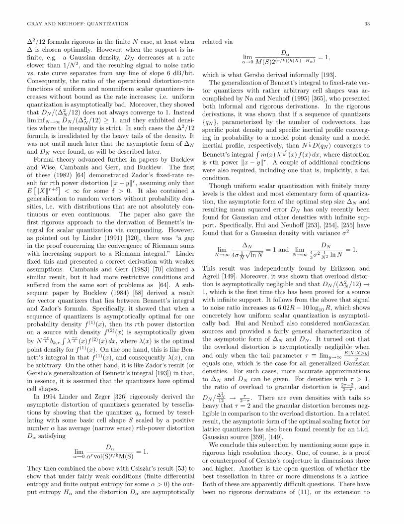
GRAY AND NEUHOFF: QUANTIZATION 33
∆2/12 formula rigorous in the finite N case, at least when∆ is chosen optimally. However, when the support is in-finite, e.g. a Gaussian density, DN decreases at a rateslower than 1/N2, and the resulting signal to noise ratiovs. rate curve separates from any line of slope 6 dB/bit.Consequently, the ratio of the operational distortion-ratefunctions of uniform and nonuniform scalar quantizers in-creases without bound as the rate increases; i.e. uniformquantization is asymptotically bad. Moreover, they showedthat DN/(∆2
N/12) does not always converge to 1. Insteadlim infN→∞DN/(∆2
N/12) ≥ 1, and they exhibited densi-ties where the inequality is strict. In such cases the ∆2/12formula is invalidated by the heavy tails of the density. Itwas not until much later that the asymptotic form of ∆N
and DN were found, as will be described later.Formal theory advanced further in papers by Bucklew
and Wise, Cambanis and Gerr, and Bucklew. The firstof these (1982) [64] demonstrated Zador’s fixed-rate re-sult for rth power distortion ‖x− y‖r, assuming only thatE[‖X‖r+δ
]< ∞ for some δ > 0. It also contained a
generalization to random vectors without probability den-sities, i.e. with distributions that are not absolutely con-tinuous or even continuous. The paper also gave thefirst rigorous approach to the derivation of Bennett’s in-tegral for scalar quantization via companding. However,as pointed out by Linder (1991) [320], there was “a gapin the proof concerning the convergence of Riemann sumswith increasing support to a Riemann integral.” Linderfixed this and presented a correct derivation with weakerassumptions. Cambanis and Gerr (1983) [70] claimed asimilar result, but it had more restrictive conditions andsuffered from the same sort of problems as [64]. A sub-sequent paper by Bucklew (1984) [58] derived a resultfor vector quantizers that lies between Bennett’s integraland Zador’s formula. Specifically, it showed that when asequence of quantizers is asymptotically optimal for oneprobability density f (1)(x), then its rth power distortionon a source with density f (2)(x) is asymptotically givenby N
−rk bk,r
∫λ−rk (x)f (2)(x) dx, where λ(x) is the optimal
point density for f (1)(x). On the one hand, this is like Ben-nett’s integral in that f (1)(x), and consequently λ(x), canbe arbitrary. On the other hand, it is like Zador’s result (orGersho’s generalization of Bennett’s integral [193]) in that,in essence, it is assumed that the quantizers have optimalcell shapes.
In 1994 Linder and Zeger [326] rigorously derived theasymptotic distortion of quantizers generated by tessella-tions by showing that the quantizer qα formed by tessel-lating with some basic cell shape S scaled by a positivenumber α has average (narrow sense) rth-power distortionDα satisfying
limα→0
Dα
αrvol(S)r/kM(S)= 1.
They then combined the above with Csiszar’s result (53) toshow that under fairly weak conditions (finite differentialentropy and finite output entropy for some α > 0) the out-put entropy Hα and the distortion Dα are asymptotically
related via
limα→0
Dα
M(S)2(r/k)(h(X)−Hα)= 1,
which is what Gersho derived informally [193].The generalization of Bennett’s integral to fixed-rate vec-
tor quantizers with rather arbitrary cell shapes was ac-complished by Na and Neuhoff (1995) [365], who presentedboth informal and rigorous derivations. In the rigorousderivations, it was shown that if a sequence of quantizers{qN}, parameterized by the number of codevectors, hasspecific point density and specific inertial profile converg-ing in probability to a model point density and a modelinertial profile, respectively, then N
rkD(qN ) converges to
Bennett’s integral∫m(x)λ
−rk (x) f(x) dx, where distortion
is rth power ‖x − y‖r. A couple of additional conditionswere also required, including one that is, implicitly, a tailcondition.
Though uniform scalar quantization with finitely manylevels is the oldest and most elementary form of quantiza-tion, the asymptotic form of the optimal step size ∆N andresulting mean squared error DN has only recently beenfound for Gaussian and other densities with infinite sup-port. Specifically, Hui and Neuhoff [253], [254], [255] havefound that for a Gaussian density with variance σ2
limN→∞
∆N
4σ 1N
√lnN
= 1 and limN→∞
DN43σ
2 1N2 lnN
= 1.
This result was independently found by Eriksson andAgrell [149]. Moreover, it was shown that overload distor-tion is asymptotically negligible and that DN/(∆2
N/12)→1, which is the first time this has been proved for a sourcewith infinite support. It follows from the above that signalto noise ratio increases as 6.02R− 10 log10R, which showsconcretely how uniform scalar quantization is asymptoti-cally bad. Hui and Neuhoff also considered nonGaussiansources and provided a fairly general characterization ofthe asymptotic form of ∆N and DN . It turned out thatthe overload distortion is asymptotically negligible whenand only when the tail parameter τ ≡ limy→∞
E[X|X>y]y
equals one, which is the case for all generalized Gaussiandensities. For such cases, more accurate approximationsto ∆N and DN can be given. For densities with τ > 1,the ratio of overload to granular distortion is 2τ−2
2−τ , and
DN/∆2N
12 → τ2−τ . There are even densities with tails so
heavy that τ = 2 and the granular distortion becomes neg-ligible in comparison to the overload distortion. In a relatedresult, the asymptotic form of the optimal scaling factor forlattice quantizers has also been found recently for an i.i.d.Gaussian source [359], [149].
We conclude this subsection by mentioning some gaps inrigorous high resolution theory. One, of course, is a proofor counterproof of Gersho’s conjecture in dimensions threeand higher. Another is the open question of whether thebest tessellation in three or more dimensions is a lattice.Both of these are apparently difficult questions. There havebeen no rigorous derivations of (11), or its extension to
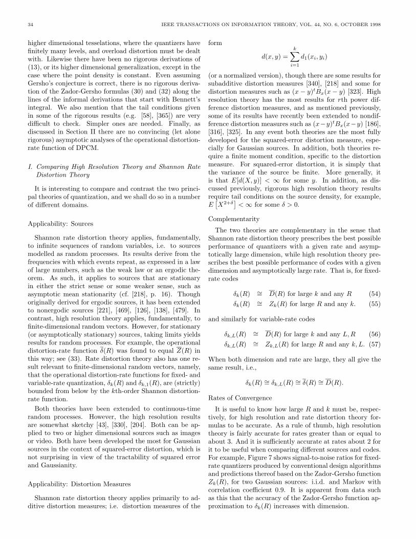
34 IEEE TRANSACTIONS ON INFORMATION THEORY, VOL. 44, NO. 6, OCTOBER 1998
higher dimensional tesselations, where the quantizers havefinitely many levels, and overload distortion must be dealtwith. Likewise there have been no rigorous derivations of(13), or its higher dimensional generalization, except in thecase where the point density is constant. Even assumingGersho’s conjecture is correct, there is no rigorous deriva-tion of the Zador-Gersho formulas (30) and (32) along thelines of the informal derivations that start with Bennett’sintegral. We also mention that the tail conditions givenin some of the rigorous results (e.g. [58], [365]) are verydifficult to check. Simpler ones are needed. Finally, asdiscussed in Section II there are no convincing (let alonerigorous) asymptotic analyses of the operational distortion-rate function of DPCM.
I. Comparing High Resolution Theory and Shannon RateDistortion Theory
It is interesting to compare and contrast the two princi-pal theories of quantization, and we shall do so in a numberof different domains.
Applicability: Sources
Shannon rate distortion theory applies, fundamentally,to infinite sequences of random variables, i.e. to sourcesmodelled as random processes. Its results derive from thefrequencies with which events repeat, as expressed in a lawof large numbers, such as the weak law or an ergodic the-orem. As such, it applies to sources that are stationaryin either the strict sense or some weaker sense, such asasymptotic mean stationarity (cf. [218], p. 16). Thoughoriginally derived for ergodic sources, it has been extendedto nonergodic sources [221], [469], [126], [138], [479]. Incontrast, high resolution theory applies, fundamentally, tofinite-dimensional random vectors. However, for stationary(or asymptotically stationary) sources, taking limits yieldsresults for random processes. For example, the operationaldistortion-rate function δ(R) was found to equal Z(R) inthis way; see (33). Rate distortion theory also has one re-sult relevant to finite-dimensional random vectors, namely,that the operational distortion-rate functions for fixed- andvariable-rate quantization, δk(R) and δk,1(R), are (strictly)bounded from below by the kth-order Shannon distortion-rate function.
Both theories have been extended to continuous-timerandom processes. However, the high resolution resultsare somewhat sketchy [43], [330], [204]. Both can be ap-plied to two or higher dimensional sources such as imagesor video. Both have been developed the most for Gaussiansources in the context of squared-error distortion, which isnot surprising in view of the tractability of squared errorand Gaussianity.
Applicability: Distortion Measures
Shannon rate distortion theory applies primarily to ad-ditive distortion measures; i.e. distortion measures of the
form
d(x, y) =k∑i=1
d1(xi, yi)
(or a normalized version), though there are some results forsubadditive distortion measures [340], [218] and some fordistortion measures such as (x− y)tBx(x− y) [323]. Highresolution theory has the most results for rth power dif-ference distortion measures, and as mentioned previously,some of its results have recently been extended to nondif-ference distortion measures such as (x−y)tBx(x−y) [186],[316], [325]. In any event both theories are the most fullydeveloped for the squared-error distortion measure, espe-cially for Gaussian sources. In addition, both theories re-quire a finite moment condition, specific to the distortionmeasure. For squared-error distortion, it is simply thatthe variance of the source be finite. More generally, itis that E[d(X, y)] < ∞ for some y. In addition, as dis-cussed previously, rigorous high resolution theory resultsrequire tail conditions on the source density, for example,E[X2+δ
]<∞ for some δ > 0.
Complementarity
The two theories are complementary in the sense thatShannon rate distortion theory prescribes the best possibleperformance of quantizers with a given rate and asymp-totically large dimension, while high resolution theory pre-scribes the best possible performance of codes with a givendimension and asymptotically large rate. That is, for fixed-rate codes
δk(R) ∼= D(R) for large k and any R (54)δk(R) ∼= Zk(R) for large R and any k. (55)
and similarly for variable-rate codes
δk,L(R) ∼= D(R) for large k and any L,R (56)δk,L(R) ∼= Zk,L(R) for large R and any k, L. (57)
When both dimension and rate are large, they all give thesame result, i.e.,
δk(R) ∼= δk,L(R) ∼= δ(R) ∼= D(R).
Rates of Convergence
It is useful to know how large R and k must be, respec-tively, for high resolution and rate distortion theory for-mulas to be accurate. As a rule of thumb, high resolutiontheory is fairly accurate for rates greater than or equal toabout 3. And it is sufficiently accurate at rates about 2 forit to be useful when comparing different sources and codes.For example, Figure 7 shows signal-to-noise ratios for fixed-rate quantizers produced by conventional design algorithmsand predictions thereof based on the Zador-Gersho functionZk(R), for two Gaussian sources: i.i.d. and Markov withcorrelation coefficient 0.9. It is apparent from data suchas this that the accuracy of the Zador-Gersho function ap-proximation to δk(R) increases with dimension.
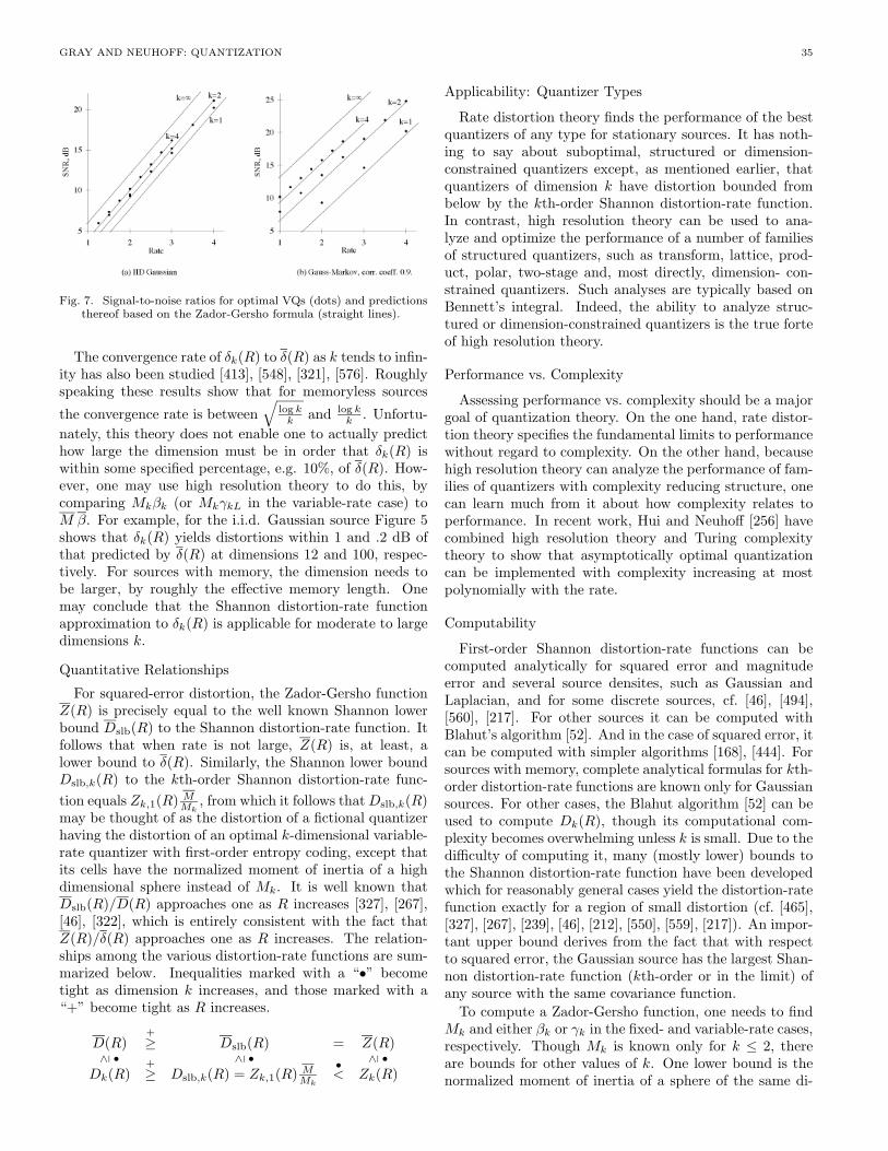
GRAY AND NEUHOFF: QUANTIZATION 35
Fig. 7. Signal-to-noise ratios for optimal VQs (dots) and predictionsthereof based on the Zador-Gersho formula (straight lines).
The convergence rate of δk(R) to δ(R) as k tends to infin-ity has also been studied [413], [548], [321], [576]. Roughlyspeaking these results show that for memoryless sources
the convergence rate is between√
log kk and log k
k . Unfortu-nately, this theory does not enable one to actually predicthow large the dimension must be in order that δk(R) iswithin some specified percentage, e.g. 10%, of δ(R). How-ever, one may use high resolution theory to do this, bycomparing Mkβk (or MkγkL in the variable-rate case) toM β. For example, for the i.i.d. Gaussian source Figure 5shows that δk(R) yields distortions within 1 and .2 dB ofthat predicted by δ(R) at dimensions 12 and 100, respec-tively. For sources with memory, the dimension needs tobe larger, by roughly the effective memory length. Onemay conclude that the Shannon distortion-rate functionapproximation to δk(R) is applicable for moderate to largedimensions k.
Quantitative Relationships
For squared-error distortion, the Zador-Gersho functionZ(R) is precisely equal to the well known Shannon lowerbound Dslb(R) to the Shannon distortion-rate function. Itfollows that when rate is not large, Z(R) is, at least, alower bound to δ(R). Similarly, the Shannon lower boundDslb,k(R) to the kth-order Shannon distortion-rate func-tion equals Zk,1(R) MMk
, from which it follows thatDslb,k(R)may be thought of as the distortion of a fictional quantizerhaving the distortion of an optimal k-dimensional variable-rate quantizer with first-order entropy coding, except thatits cells have the normalized moment of inertia of a highdimensional sphere instead of Mk. It is well known thatDslb(R)/D(R) approaches one as R increases [327], [267],[46], [322], which is entirely consistent with the fact thatZ(R)/δ(R) approaches one as R increases. The relation-ships among the various distortion-rate functions are sum-marized below. Inequalities marked with a “•” becometight as dimension k increases, and those marked with a“+” become tight as R increases.
D(R)+≥ Dslb(R) = Z(R)
≥ • ≥ • ≥ •
Dk(R)+≥ Dslb,k(R) = Zk,1(R) MMk
•< Zk(R)
Applicability: Quantizer Types
Rate distortion theory finds the performance of the bestquantizers of any type for stationary sources. It has noth-ing to say about suboptimal, structured or dimension-constrained quantizers except, as mentioned earlier, thatquantizers of dimension k have distortion bounded frombelow by the kth-order Shannon distortion-rate function.In contrast, high resolution theory can be used to ana-lyze and optimize the performance of a number of familiesof structured quantizers, such as transform, lattice, prod-uct, polar, two-stage and, most directly, dimension- con-strained quantizers. Such analyses are typically based onBennett’s integral. Indeed, the ability to analyze struc-tured or dimension-constrained quantizers is the true forteof high resolution theory.
Performance vs. Complexity
Assessing performance vs. complexity should be a majorgoal of quantization theory. On the one hand, rate distor-tion theory specifies the fundamental limits to performancewithout regard to complexity. On the other hand, becausehigh resolution theory can analyze the performance of fam-ilies of quantizers with complexity reducing structure, onecan learn much from it about how complexity relates toperformance. In recent work, Hui and Neuhoff [256] havecombined high resolution theory and Turing complexitytheory to show that asymptotically optimal quantizationcan be implemented with complexity increasing at mostpolynomially with the rate.
Computability
First-order Shannon distortion-rate functions can becomputed analytically for squared error and magnitudeerror and several source densites, such as Gaussian andLaplacian, and for some discrete sources, cf. [46], [494],[560], [217]. For other sources it can be computed withBlahut’s algorithm [52]. And in the case of squared error, itcan be computed with simpler algorithms [168], [444]. Forsources with memory, complete analytical formulas for kth-order distortion-rate functions are known only for Gaussiansources. For other cases, the Blahut algorithm [52] can beused to compute Dk(R), though its computational com-plexity becomes overwhelming unless k is small. Due to thedifficulty of computing it, many (mostly lower) bounds tothe Shannon distortion-rate function have been developedwhich for reasonably general cases yield the distortion-ratefunction exactly for a region of small distortion (cf. [465],[327], [267], [239], [46], [212], [550], [559], [217]). An impor-tant upper bound derives from the fact that with respectto squared error, the Gaussian source has the largest Shan-non distortion-rate function (kth-order or in the limit) ofany source with the same covariance function.
To compute a Zador-Gersho function, one needs to findMk and either βk or γk in the fixed- and variable-rate cases,respectively. Though Mk is known only for k ≤ 2, thereare bounds for other values of k. One lower bound is thenormalized moment of inertia of a sphere of the same di-
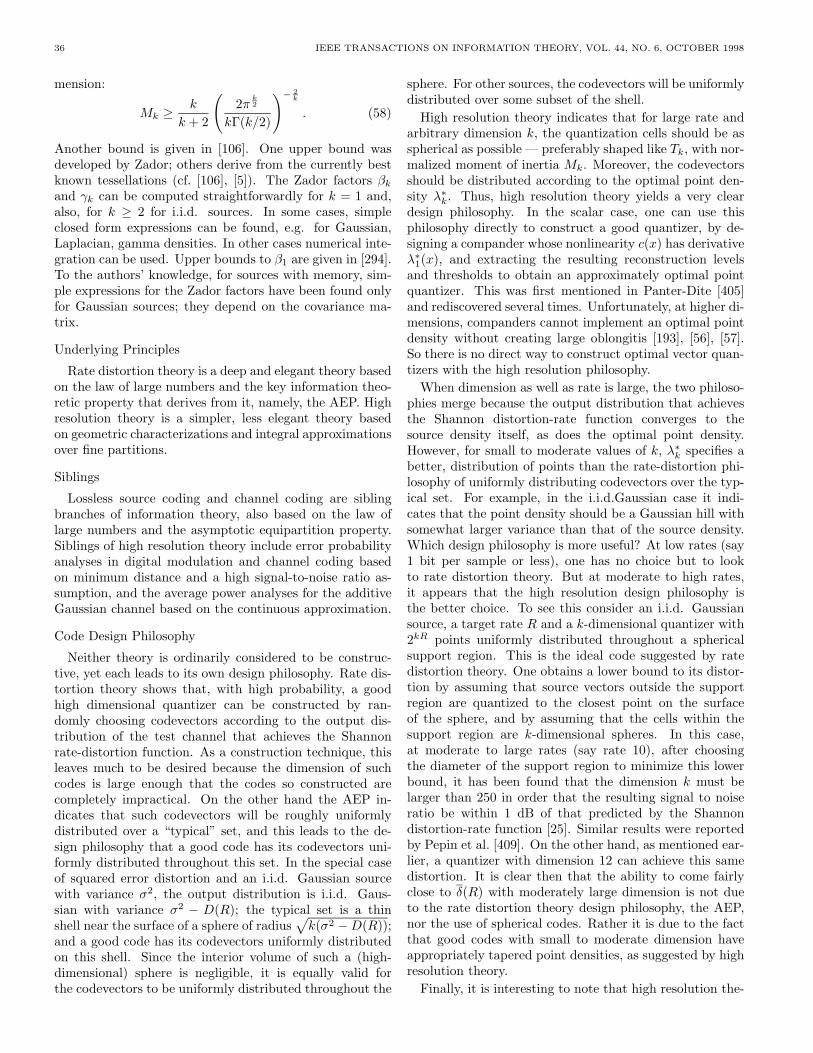
36 IEEE TRANSACTIONS ON INFORMATION THEORY, VOL. 44, NO. 6, OCTOBER 1998
mension:
Mk ≥k
k + 2
(2π
k2
kΓ(k/2)
)− 2k
. (58)
Another bound is given in [106]. One upper bound wasdeveloped by Zador; others derive from the currently bestknown tessellations (cf. [106], [5]). The Zador factors βkand γk can be computed straightforwardly for k = 1 and,also, for k ≥ 2 for i.i.d. sources. In some cases, simpleclosed form expressions can be found, e.g. for Gaussian,Laplacian, gamma densities. In other cases numerical inte-gration can be used. Upper bounds to β1 are given in [294].To the authors’ knowledge, for sources with memory, sim-ple expressions for the Zador factors have been found onlyfor Gaussian sources; they depend on the covariance ma-trix.
Underlying Principles
Rate distortion theory is a deep and elegant theory basedon the law of large numbers and the key information theo-retic property that derives from it, namely, the AEP. Highresolution theory is a simpler, less elegant theory basedon geometric characterizations and integral approximationsover fine partitions.
Siblings
Lossless source coding and channel coding are siblingbranches of information theory, also based on the law oflarge numbers and the asymptotic equipartition property.Siblings of high resolution theory include error probabilityanalyses in digital modulation and channel coding basedon minimum distance and a high signal-to-noise ratio as-sumption, and the average power analyses for the additiveGaussian channel based on the continuous approximation.
Code Design Philosophy
Neither theory is ordinarily considered to be construc-tive, yet each leads to its own design philosophy. Rate dis-tortion theory shows that, with high probability, a goodhigh dimensional quantizer can be constructed by ran-domly choosing codevectors according to the output dis-tribution of the test channel that achieves the Shannonrate-distortion function. As a construction technique, thisleaves much to be desired because the dimension of suchcodes is large enough that the codes so constructed arecompletely impractical. On the other hand the AEP in-dicates that such codevectors will be roughly uniformlydistributed over a “typical” set, and this leads to the de-sign philosophy that a good code has its codevectors uni-formly distributed throughout this set. In the special caseof squared error distortion and an i.i.d. Gaussian sourcewith variance σ2, the output distribution is i.i.d. Gaus-sian with variance σ2 − D(R); the typical set is a thinshell near the surface of a sphere of radius
√k(σ2 −D(R));
and a good code has its codevectors uniformly distributedon this shell. Since the interior volume of such a (high-dimensional) sphere is negligible, it is equally valid forthe codevectors to be uniformly distributed throughout the
sphere. For other sources, the codevectors will be uniformlydistributed over some subset of the shell.
High resolution theory indicates that for large rate andarbitrary dimension k, the quantization cells should be asspherical as possible — preferably shaped like Tk, with nor-malized moment of inertia Mk. Moreover, the codevectorsshould be distributed according to the optimal point den-sity λ∗k. Thus, high resolution theory yields a very cleardesign philosophy. In the scalar case, one can use thisphilosophy directly to construct a good quantizer, by de-signing a compander whose nonlinearity c(x) has derivativeλ∗1(x), and extracting the resulting reconstruction levelsand thresholds to obtain an approximately optimal pointquantizer. This was first mentioned in Panter-Dite [405]and rediscovered several times. Unfortunately, at higher di-mensions, companders cannot implement an optimal pointdensity without creating large oblongitis [193], [56], [57].So there is no direct way to construct optimal vector quan-tizers with the high resolution philosophy.
When dimension as well as rate is large, the two philoso-phies merge because the output distribution that achievesthe Shannon distortion-rate function converges to thesource density itself, as does the optimal point density.However, for small to moderate values of k, λ∗k specifies abetter, distribution of points than the rate-distortion phi-losophy of uniformly distributing codevectors over the typ-ical set. For example, in the i.i.d.Gaussian case it indi-cates that the point density should be a Gaussian hill withsomewhat larger variance than that of the source density.Which design philosophy is more useful? At low rates (say1 bit per sample or less), one has no choice but to lookto rate distortion theory. But at moderate to high rates,it appears that the high resolution design philosophy isthe better choice. To see this consider an i.i.d. Gaussiansource, a target rate R and a k-dimensional quantizer with2kR points uniformly distributed throughout a sphericalsupport region. This is the ideal code suggested by ratedistortion theory. One obtains a lower bound to its distor-tion by assuming that source vectors outside the supportregion are quantized to the closest point on the surfaceof the sphere, and by assuming that the cells within thesupport region are k-dimensional spheres. In this case,at moderate to large rates (say rate 10), after choosingthe diameter of the support region to minimize this lowerbound, it has been found that the dimension k must belarger than 250 in order that the resulting signal to noiseratio be within 1 dB of that predicted by the Shannondistortion-rate function [25]. Similar results were reportedby Pepin et al. [409]. On the other hand, as mentioned ear-lier, a quantizer with dimension 12 can achieve this samedistortion. It is clear then that the ability to come fairlyclose to δ(R) with moderately large dimension is not dueto the rate distortion theory design philosophy, the AEP,nor the use of spherical codes. Rather it is due to the factthat good codes with small to moderate dimension haveappropriately tapered point densities, as suggested by highresolution theory.
Finally, it is interesting to note that high resolution the-
GRAY AND NEUHOFF: QUANTIZATION 37
ory actually contains some analyses of the Shannon randomcoding approach. For example, Zador’s thesis [561] givesan upper bound on the distortion of a randomly generatedvector quantizer.
Nature of the Error Process
Both theories have something to say about the distri-bution of quantization errors. Generally speaking, whatrate distortion theory has to say comes from assuming thatthe error distribution caused by a quantizer whose per-formance is close to δ(R) is similar to that caused by atest channel that comes close to achieving the Shannondistortion-rate function. This is reasonable because Shan-non’s random coding argument shows that using such atest channel to randomly generate high dimensional code-vectors leads, with very high probability, to a code whosedistortion is close to δ(R). For example, one may use thissort of argument to deduce that the quantization error ofa good high dimensional quantizer is approximately whiteand Gaussian when the source is memoryless, the distor-tion is squared error, and the rate is large, cf. [404], whichshows Gaussian-like histograms for the quantization errorof VQ’s with dimensions 8 to 32. As another example, fora Gaussian source with memory and squared-error distor-tion, rate distortion theory shows there is a simple relationbetween the spectra of the source and the spectra of theerror produced by an optimal high dimensional quantizer,cf. [46].
High resolution theory also has a long tradition of ana-lyzing the error process, beginning with Clavier et al. [99],[100] and Bennett [43] and focusing on the distribution ofthe error, its spectrum and its correlation with the input.Bennett showed that in the high resolution case, the powerspectral density of the quantizer error with uniform quanti-zation is approximately white (and uniformly distributed)provided the assumptions of the high resolution theoryare met and the joint density of sample pairs is smooth.(See also Section 5.6 of [196].) Bennett also found exactexpressions for the power spectral density of a uniformlyquantized Gaussian process. Sripad and Snyder [477] andClaasen and Jongepier [97] derived conditions under whichthe quantization error is white in terms of the joint char-acteristic functions of pairs of samples, two-dimensionalanalogs of Widrow’s [529] condition. Zador [562] foundhigh resolution expressions for the characteristic function ofthe error produced by randomly chosen vector quantizers.Lee and Neuhoff [312], [379] found high resolution expres-sions for the density of the error produced by fairly gen-eral (deterministic) scalar and vector quantizers in termsof their point density and their shape profile, which is afunction that conveys more cell shape information than theinertial profile. As a side benefit, these expressions indicatethat much can be deduced about the point density and cellshapes of a quantizer from a histogram of the lengths of theerrors. Zamir and Feder [564] showed that the error pro-duced by an optimal lattice quantizer with infinitely manysmall cells is asymptotically white in the sense that itscomponents are uncorrelated with zero means and identical
variances. Moreover they showed that it becomes Gaussianas the dimension increases. The basic ideas are that as di-mension increases good lattices have nearly spherical cellsand that a uniform distribution over a high dimensionalsphere is approximately Gaussian, cf. [525]. Since optimalhigh dimensional, high rate VQs can also be expected tohave nearly spherical cells and since the AEP implies thatmost cells will have the same size, we reach the same con-clusion as from rate distortion theory, namely that goodhigh-rate, high-dimensional codes cause the quantizationerror to be approximately white and Gaussian.
Successive Approximation
Many vector quantizers operate in a successive approx-imation or progressive fashion, whereby a low rate coarsequantization is followed by a sequence of finer and finerquantizations, which add to the rate. Tree-structured, mul-tistage and hierarchical quantizers, to be discussed in thenext section, are examples of such. Other methods can beused to design progressive indexing into given codebooks,as in Yamada and Tazaki (1991) [553] and Riskin et al.(1994) [440]
Successive approximation is useful in situations wherethe decoder needs to produce rough approximations of thedata from the first bits it receives and, subsequently, torefine the approximation as more bits are received. More-over, successive approximation quantizers are often struc-tured in a way that makes them simpler than unstructuredones. Indeed, the three examples just cited are known morefor their good performance with low complexity than fortheir progressive nature. An important question is whetherthe performance of a successive refinement quantizer willbe better than one that does quantization in one step. Onthe one hand, rate distortion theory analysis [228], [291],[292], [557], [147], [437], [96] has shown that there are sit-uations where successive approximation can be done with-out loss of optimality. On the other hand, high resolutionanalyses of TSVQ [383] and two-stage VQ [311] have quan-tified the loss of these particular codes, and in the lattercase shown ways of modifying the quantizer to eliminatethe loss. Thus, both theories have something to say aboutsuccessive refinement.
V. Quantization Techniques
This section presents an overview of quantization tech-niques (mainly vector) that have been introduced, begin-ning in the 1980’s, with the goal of attaining rate/distortionperformance better than that attainable by scalar basedtechniques such as direct scalar quantization, DPCM, andtransform coding, but without the inordinately large com-plexity of brute force vector quantization methods. Recallthat if the dimension of the source vector is fixed, say atk, then the goal is to attain performance close to the op-timal performance as expressed by δk(R) in the fixed ratecase, or δk,L(R) (usually δk,1(R)) in the general case wherevariable-rate codes are permitted. However if, as in thecase of a stationary source, the dimension k can be chosenarbitrarily, then in both the fixed and variable-rate cases,
38 IEEE TRANSACTIONS ON INFORMATION THEORY, VOL. 44, NO. 6, OCTOBER 1998
the goal is to attain performance close to δ(R). In this caseall quantizers with R > 0 are suboptimal, and quantizerswith various dimensions and even memory (which blurs thenotion of dimension) can be considered.
We would have liked to make a carefully categorized,ordered and ranked presentation of the various methods.However, the literature and variety of such techniques isquite large; there are a number of competing ways in whichto categorize the techniques; complexity is itself a difficultthing to quantify; there are several special cases (e.g. fixedor variable rate, and fixed or choosable dimension); andthere has not been much theoretical or even quantitativecomparison among them. Consequently, much work is stillneeded in sorting the wheat from the chaff, i.e. determiningwhich methods give the best performance vs. complexitytradeoff in which situations, and in gaining an understand-ing of why certain complexity reducing approaches are bet-ter than others. Nevertheless we have attempted to choosea reasonable set of techniques and an ordering of them fordiscussion. Where possible we will make comments aboutthe efficacies of the techniques. In all cases, we includereferences.
We begin with a brief discussion of complexity. Roughlyspeaking it has two aspects: arithmetic (or computational)complexity, which is the number of arithmetic operationsper sample that must be performed when encoding ordecoding, and storage (or memory or space) complexity,which is the amount of auxiliary storage (for exampleof codebooks) that is required for encoding or decoding.Rather than trying to combine them, it makes sense tokeep separate track, because their associated costs varywith implementation venue, e.g. a PC, UNIX platform,generic DSP chip, specially designed VLSI chip, etc. Insome venues, storage is of such low cost that one is temptedto ignore it. However, there are techniques that benefit suf-ficiently from increased memory that even though the perunit cost is trivial, to obtain the best performance com-plexity tradeoff, memory usage should be increased untilthe marginal gain-to-cost ratio of further increases is small,at which point the total cost of memory may be signficant.As a result one might think of a quantizer as being charac-terized by a four-tuple (R,D,A,M); i.e. arithmetic com-plexity A and storage complexity M have been added tothe usual rate R and distortion D.
As a reminder, given a k-dimensional fixed-rate VQ withcodebook C containing 2kR codevectors, brute force fullsearch encoding finds the closest codevector in C by com-puting the distortion between x and each codevector. Inother words, it uses the optimal lossy encoder for the givencodebook, creating the Voronoi partition. In the caseof squared error, this requires computing approximatelyA = 3 × 2kR operations per sample and storing approx-imately M = k × 2kR vector components. For example,a codebook with rate .25 bits per pixel (bpp) and vectordimension 8 × 8 = 64 has 2kR = 216 codevectors, an im-practical number for, say, real time video coding. This ex-ponential explosion of complexity and memory can causeserious problems even for modest dimension and rate, but
it can in general make codes completely impractical in ei-ther the high resolution or high dimension extremes. Abrute force variable-rate scheme of the same rate will beeven more complex — typically involving a much greaternumber of codevectors, a Lagrangian distortion computa-tion, and an entropy coding scheme as well. It is the highcomplexity of such brute force techniques that motivatesthe reduced complexity techniques to be discussed later inthis section.
Simple measures such as arithmetic complexity and stor-age need a number of qualifications. One must decidewhether encoding and decoding complexities need to becounted separately or summed, or indeed whether only oneof them is important. For example, in record-once-play-many situations, it is the decoder that must have low com-plexity. Having no particular application in mind, we willfocus on the sum of encoder and decoder complexities. Forsome techniques (perhaps most) it is possible to trade com-putations for storage by the use of precomputed tables. Insuch cases a quantizer is characterized, not by a single Aand M but by a curve of such. In some cases, a given setof precomputed tables is the heart of the method. Anotherissue is the cost of memory accesses. Such operations areusually signficantly less expensive than arithmetic opera-tions. However, some methods do such a good job of reduc-ing arithmetic operations that the cost of memory accessesbecomes significant. Techniques that attain smaller valuesof distortion need higher precision in their arithmetic andstorage, which though not usually accounted for in assess-ments of complexity may sometimes be of significance. Forexample, a recent study of VQ codebook storage has shownthat in routine cases one needs to store codevector compo-nents with only about R+4 bits per component, where R isthe rate of the quantizer [252]. Though this study did notassess the required arithmetic precision, one would guessthat it need not be more than a little larger than that ofthe storage; e.g. R plus 5 or 6 bit arithmetic should suf-fice. Finally, variable-rate coding raises additional issuessuch as the costs associated with buffering, with storingand accessing variable-length codewords, and with the de-coder having to parse binary sequences into variable-lengthcodewords.
When assessing complexity of a quantization technique,it is interesting to compare the complexity invested inthe lossy encoder/decoder vs. that in the lossless en-coder/decoder. (Recall that good performance can the-oretically be attained with either a simple lossy encoder,such as a uniform scalar quantizer, and a sophisticated loss-less encoder or vice versa, as in high dimensional fixed-rateVQ.) A quantizer is considered to have low complexity onlywhen both encoders have low complexity. In the discussionthat follows we focus mainly on quantization techniqueswhere the lossless encoder is conceptually if not quantita-tively simple. We wish, however, to mention the indexingproblem, which may be considered to lie between the loss-less and the lossy encoder. There are certain fixed-ratetechniques such as lattice quantization, pyramid VQ, andscalar-vector quantization, where it is fairly easy to find
GRAY AND NEUHOFF: QUANTIZATION 39
the cell in which the source vector lies, but the cells areassociated with some set of N indices that are not simplythe integers from 1 to N , where N is the number of cells,and converting the identity of the cell into a sequence oflogN bits is nontrivial. This is referred to as an indexingproblem.
Finally, we mention two additional issues. The first isthat there are some VQ techniques whose implementationcomplexities are not prohibitive, but which have sufficientlymany codevectors that designing them is inordinately com-plex or requires an inordinate amount of training data. Asecond issue is that in some applications it is desirable thatthe output of the encoder be progressively decodable in thesense that a rough reproduction can be made from the firstbits that it receives, and improved reproductions are madeas more bits are received. Such quantizers are said to beprogressive or embedded. Now it is true that a progressivedecoder can be designed for any encoder (for example, itcan compute the expected value of the source vector givenwhatever bits it has received so far). However, a “good”progressive code is one for which the intermediate distor-tions achieved at the intermediate rates are relatively good(though not usually as good as those of quantizers designedfor one specific rate) and that rather than restarting fromscratch every time the decoder receives a new bit (or groupof bits), it uses some simple method to update the currentreproduction. It is also desirable in some applications forthe encoding to be progressive, as well. Though not de-signed with them in mind, it turns out that a number ofthe reduced complexity VQ approaches also address theselast two issues. That is, they are easier to design, as wellas progressive.
A. Fast Searches of Unstructured Codebooks
Many techniques have been developed for speeding thefull (minimum distortion) search of an arbitrary codebookC containing N k-dimensional codevectors, for exampleone generated by a Lloyd algorithm. In contrast to code-books to be considered later these will be called unstruc-tured. As a group these techniques use substantial amountsof additional memory in order to significantly reduce arith-metic complexity. A variety of such techniques are men-tioned in Section 12.16 of [196].
A number of fast search techniques are similar in spirit tothe following: the Euclidean distances between all pairs ofcodevectors are precomputed and stored in a table. Now,given a source vector x to quantize, some initial codevectory is chosen. Then all codevectors yi whose distance from yis greater than 2‖x− y‖ are eliminated from further consid-eration because they cannot be closer than y. Those noteliminated are successively compared to x until one thatis closer than y is found, which then replaces y, and theprocess continues. In this way the set of potential code-vectors is gradually narrowed. Techniques in this category,with different ways of narrowing the search, may be foundin [362], [517], [475], [476], [363], [426], [249], [399], [273],[245], [229], [332], [307], [547], [308], [493].
A number of other fast search techniques begin with a
“coarse” prequantization with some very low complexitytechnique. It is called “coarse” because it typically haslarger cells than the Voronoi regions of the codebook Cthat is being searched. The coarse prequantization of-ten involves scalar quantization of some type or a tree-structuring of binary quantizers, such as what are calledK-d trees. Associated with each coarse cell is a bucket con-taining the indices of each codevector that is the nearestcodevector to some source vector in the cell. These buck-ets are determined in advance and saved as tables. Thento encode a source vector x, one applies the prequantiza-tion, finds the index of the prequantization cell in which xis contained, and performs a full search on the correspond-ing bucket for the closest codevector to x. Techniques ofthis type may be found in [44], [176], [88], [89], [334], [146],[532], [423], [415], [500], [84]. In some of these, the coarseprequantization is one-dimensional; for example, the lengthof the source vector may be quantized, and then the bucketof all codevectors having similar lengths is searched for theclosest codevector.
Another class of techniques is like the previous exceptthat the low complexity prequantization has much smallercells than the Voronoi cells of C, i.e. it is finer. In thiscase, the buckets associated with most “fine” prequantiza-tion cells contain just one codevector, i.e. the same code-vector in C is the closest codevector to each point in thefine cell. The indices of these codevectors, one for eachfine cell, are stored in a precomputed table. For each ofthose relatively few fine cells that have buckets contain-ing more than one codevector, one member of the bucketis chosen and its index is placed in the table as the entryfor that fine cell. Quantization of x then proceeds by ap-plying the fine prequantizer and then using the index ofthe fine cell in which x lies to address the table contain-ing codevectors from C, which then outputs the index ofa codeword in C. Due to the fact that not every bucketcontains only one codevector, such techniques, which maybe found in [86], [358], [357], [518], [75], [219], do not doa perfect full search. Some quantitative analysis of theincreased distortion is given in [356] for a case where theprequantization is a lattice quantizer. Other fast searchmethods include the partial distortion method of [88], [39],[402] and the transform subspace domain approach of [78].
Consideration of methods based on prequantization leadsto the question of how fine the prequantization cells shouldbe. Our experience is that the best tradeoffs come whenthe prequantization cells are finer rather than coarser, theexplanation being that if one has prequantized coarsely andnow has to determine which codevector in a bucket is clos-est to x, it is more efficient to use some fast search methodthan to do full search. Dividing the coarse cells into finerones is a way of doing just this. Another question thatarises for all fast search techniques is whether it is worth theeffort to perform a full search or whether one should insteadstop short of this, as in the methods with fine prequantiza-tion cells. Our experience is that it is usually not worth theeffort to do a full search, because by suffering only a verysmall increase in MSE one can achieve a significant reduc-
40 IEEE TRANSACTIONS ON INFORMATION THEORY, VOL. 44, NO. 6, OCTOBER 1998
tion in arithmetic complexity and storage. Moreover, in thecase of stationary sources where the dimension is subjectto choice, for a given amount of arithmetic complexity andstorage, one almost always gets better performance by do-ing a suboptimal search of a higher dimensional codebookthan a full search of a lower dimensional one.
Fast search methods based on fine prequantization canbe improved by optimizing the codebook for the given pre-quantizer. Each cell of the partition corresponding to Cinduced by prequantization followed by table lookup is theunion of some number fine cells of the prequantizer. Thusthe question becomes: what is the best partition into Ncells, each of which is the union of some number of fine cells.The codevectors in C should then be the centroids of thesecells. Such techniques have been exploited in [86], [358].One technique worth particular mention is called hierar-chical table lookup VQ [86], [518], [75], [219]. In this case,the prequantizer is itself an unstructured codebook that issearched with a fine prequantizer that is in turn searchedwith an even finer prequantizer, and so on. Specifically, thefirst prequantizer uses a high rate scalar quantizer k times.The next level of prequantization applies a two-dimensionalVQ to each of k/2 pairs of scalar quantizer outputs. Thenext level applies a four-dimensional VQ to each of k/4pairs of outputs from the two-dimensional quantizers, andso on. Hence the method is hierarchical. Because eachof the quantizers can be implemented entirely with tablelook up, this method eliminates all arithmetic complexityexcept memory accesses. It has been successfully used forvideo coding [518], [75].
B. Structured Quantizers
We now turn to quantizers with structured partitionsor reproduction codebooks, which in turn lend themselvesto fast searching techniques and, in some cases, to greatlyreduced storage. Many of these techniques are discussedin [196], [458].
Lattice Quantizers
Lattice quantization can be viewed as a vector general-ization of uniform scalar quantization. It constrains thereproduction codebook to be a subset of a regular lat-tice, where a lattice is the set of all vectors of the form∑ni=1miui, where mi are integers and the ui are linearly
independent (usually nondegenerate, i.e., n = k). The re-sulting Voronoi partition is a tessellation with all cells (ex-cept for those overlapping the overload region) having thesame shape, size and orientation. Lattice quantization wasproposed by Gersho [193] because of its near optimalityfor high resolution variable-rate quantization and, also, itsnear optimality for high resolution fixed-rate quantizationof uniformly distributed sources. (These assume that Ger-sho’s conjecture holds and that the best lattice quantizeris approximately as good as the best tessellation.) Espe-cially important is the fact that their highly structurednature has lead to algorithms for implementing their lossyencoders with very low arithmetic and stoarge complexi-ties [103], [104], [105], [459], [106], [199]. These find the
integers mi associated with the closest lattice point. Con-way and Sloane [104], [106] have reported the best knownlattices for several dimensions, as well as fast quantizingand decoding algorithms. Some important n-dimensionallattices are the root lattices An(n ≥ 1), Dn(n ≥ 2), andEn(n = 6, 7, 8), the Barnes-Wall lattice Λ16 in dimension16, and the Leech lattice Λ24 in 24 dimensions. These lat-ter give the best sphere packings and coverings in theirrespective dimensions. Recently, Agrell and Eriksson [5]have found improved lattices in dimensions 9 and 10.
Though low complexity algorithms have been found forthe lossy encoder, there are other issues that affect theperformance and complexity of lattice quantizers. Forvariable-rate coding, one must scale the lattice to obtainthe desired distortion and rate, and one must implementan algorithm for mapping the mi’s to the variable-lengthbinary codewords. The latter could potentially add muchcomplexity. For fixed-rate coding with rate R, the latticemust be scaled and a subset of 2kR lattice points mustbe identified as the codevectors. This induces a supportregion. If the source has finite support, the lattice quan-tizer will ordinarily be chosen to have the same support. Ifnot, then the scaling factor and lattice subset are usuallychosen so that the resulting quantizer support region haslarge probability. In either case a low complexity method isneeded for assigning binary sequences to the chosen code-vectors; i.e. for indexing. Conway and Sloane [105] foundsuch a method for the important case that the support hasthe shape of an enlarged cell. For sources with infinitesupport, such as i.i.d. Gaussian, there is also the difficultquestion of how to quantize a source vector x lying out-side the support region. For example, one might scale x sothat it lies on or just inside the boundary of the supportregion, and then quantize the scaled vector in the usualway. Unfortunately, this simple method does not alwaysfind the closest codevector to x. Indeed, it often increasesoverload distortion substantially over that of the minimum-distance quantization rule. To date, there is apparently nolow complexity method that does not substantially increaseoverload distortion.
High resolution theory applies immediately to lattice VQwhen the entire lattice is considered to be the codebook.The theory becomes more difficult if, as is usually the case,only a bounded portion of the lattice is used as the code-book and one must separately consider granular and over-load distortion. There are a variety of ways of consideringthe tradeoffs involved, cf. [580], [151], [359], [149], [409].In any case, the essence of a lattice code is its uniformpoint density and nicely shaped cells with low normalizedmoment of inertia. For fixed-rate coding, they work wellfor uniform sources or other sources with bounded sup-port. But as discussed earlier, for sources with unboundedsupport such as i.i.d. Gaussian, they require very largedimensions to achieve performance close to δ(R).
Product Quantizers
A product quantizer uses a reproduction codebook thatis the cartesian product of lower dimensional reproduction
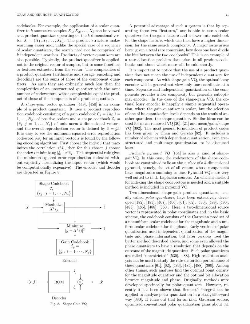
GRAY AND NEUHOFF: QUANTIZATION 41
codebooks. For example, the application of a scalar quan-tizer to k successive samples X1, X2, . . . , Xk can be viewedas a product quantizer operating on the k-dimensional vec-tor X = (X1, X2, . . . , Xk). The product structure makessearching easier and, unlike the special case of a sequenceof scalar quantizers, the search need not be comprised ofk independent searches. Products of vector quantizers arealso possible. Typically, the product quantizer is applied,not to the original vector of samples, but to some functionsor features extracted from the vector. The complexities ofa product quantizer (arithmetic and storage, encoding anddecoding) are the sums of those of the component quan-tizers. As such they are ordinarily much less than thecomplexities of an unstructured quantizer with the samenumber of codevectors, whose complexities equal the prod-uct of those of the components of a product quantizer.
A shape-gain vector quantizer [449], [450] is an exam-ple of a product quantizer. It uses a product reproduc-tion codebook consisting of a gain codebook Cg = {gi; i =1, . . . , Ng} of positive scalars and a shape codebook Cs ={sj ; j = 1, . . . , Ns} of unit norm k-dimensional vectors,and the overall reproduction vector is defined by x = gs.It is easy to see the minimum squared error reproductioncodeword gisj for an input vector x is found by the follow-ing encoding algorithm: First choose the index j that max-imizes the correlation xtsj , then for this chosen j choosethe index i minimizing |gi−xtsj |. This sequential rule givesthe minimum squared error reproduction codeword with-out explicitly normalizing the input vector (which wouldbe computationally expensive). The encoder and decoderare depicted in Figure 8.
?
Shape CodebookCs =
{sj ; j = 1, · · · , Ns}
X - MaximizeXtsj
- j
?- Minimize
[g −Xts)]2- i
Gain CodebookCg =
{gi; i = 1, · · · , Ng}
6
Encoder
(i, j) - ROM6
?
sj
gi
l× - X
DecoderFig. 8. Shape-Gain VQ
A potential advantage of such a system is that by sep-arating these two “features,” one is able to use a scalarquantizer for the gain feature and a lower rate codebookfor the shape feature, which can then have a higher dimen-sion, for the same search complexity. A major issue ariseshere: given a total rate constraint, how does one best dividethe bits between the two codebooks? This is an example ofa rate allocation problem that arises in all product code-books and about which more will be said shortly.
It is important to notice that the use of a product quan-tizer does not mean the use of independent quantizers foreach component. As with shape-gain VQ, the optimal lossyencoder will in general not view only one coordinate at atime. Separate and independent quantization of the com-ponents provides a low complexity but generally subopti-mal encoder. In the case of the shape-gain VQ, the op-timal lossy encoder is happily a simple sequential opera-tion, where the gain quantizer is scalar, but the selectionof one of its quantization levels depends on the result of an-other quantizer, the shape quantizer. Similar ideas can beused for mean-removed VQ [20], [21] and mean/gain/shapeVQ [392]. The most general formulation of product codeshas been given by Chan and Gersho [82]. It includes anumber of schemes with dependent quantization, even tree-structured and multistage quantization, to be discussedlater.
Fischer’s pyramid VQ [164] is also a kind of shape-gainVQ. In this case, the codevectors of the shape code-book are constrained to lie on the surface of a k-dimensionalpyramid, namely, the set of all vectors whose componentshave magnitudes summing to one. Pyramid VQ’s are verywell suited to i.i.d. Laplacian sources. An efficient methodfor indexing the shape codevectors is needed and a suitablemethod is included in pyramid VQ.
Two-dimensional shape-gain product quantizers, usu-ally called polar quantizers, have been extensively devel-oped [182], [183], [407], [406], [61], [62], [530], [489], [490],[483], [485], [488], [360]. Here, a two-dimensional sourcevector is represented in polar coordinates and, in the basicscheme, the codebook consists of the Cartesian product ofa nonuniform scalar codebook for the magnitude and a uni-form scalar codebook for the phase. Early versions of polarquantization used independent quantization of the magni-tude and phase information, but later versions used thebetter method described above, and some even allowed thephase quantizers to have a resolution that depends on theoutcome of the magnitude quantizer. Such polar quantizersare called “unrestricted” [530], [488]. High resolution anal-ysis can be used to study the rate-distortion performance ofthese quantizers [61], [62], [483], [485], [488], [360]. Amongother things, such analyses find the optimal point densityfor the magnitude quantizer and the optimal bit allocationbetween magnitude and phase. Originally, methods weredeveloped specifically for polar quantizers. However, re-cently it has been shown that Bennett’s integral can beapplied to analyze polar quantization in a straightforwardway [380]. It turns out that for an i.i.d. Gaussian source,optimized conventional polar quantization gains about .41
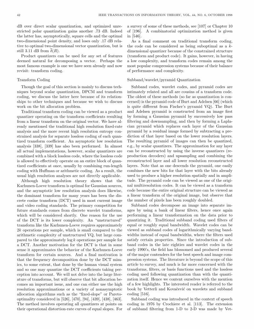
42 IEEE TRANSACTIONS ON INFORMATION THEORY, VOL. 44, NO. 6, OCTOBER 1998
dB over direct scalar quantization, and optimized unre-stricted polar quantization gains another .73 dB. Indeedthe latter has, asymptotically, square cells and the optimaltwo-dimensional point density, and loses only .17 dB rela-tive to optimal two-dimensional vector quantization, but isstill 3.11 dB from δ(R).
Product quantizers can be used for any set of featuresdeemed natural for decomposing a vector. Perhaps themost famous example is one we have seen already and nowrevisit: transform coding.
Transform Coding
Though the goal of this section is mainly to discuss tech-niques beyond scalar quantization, DPCM and transformcoding, we discuss the latter here because of its relation-ships to other techniques and because we wish to discusswork on the bit allocation problem.
Traditional transform coding can be viewed as a productquantizer operating on the transform coefficients resultingfrom a linear transform on the original vector. We have al-ready mentioned the traditional high resolution fixed-rateanalysis and the more recent high resolution entropy con-strained analysis for separate lossless coding of each quan-tized transform coefficient. An asymptotic low resolutionanalysis [338], [339] has also been performed. In almostall actual implementations, however, scalar quantizers arecombined with a block lossless code, where the lossless codeis allowed to effectively operate on an entire block of quan-tized coefficients at once, usually by combining run-lengthcoding with Huffman or arithmetic coding. As a result, theusual high resolution analyses are not directly applicable.
Although high resolution theory shows that theKarhunen-Loeve transform is optimal for Gaussian sources,and the asymptotic low resolution analysis does likewise,the dominant transform for many years has been the dis-crete cosine transform (DCT) used in most current imageand video coding standards. The primary competition forfuture standards comes from discrete wavelet transforms,which will be considered shortly. One reason for the useof the DCT is its lower complexity. An “unstructured”transform like the Karhunen-Loeve requires approximately2k operations per sample, which is small compared to thearithmetic complexity of unstructured VQ, but large com-pared to the approximately log k operations per sample fora DCT. Another motivation for the DCT is that in somesense it approximates the behavior of the Karhunen-Loevetransform for certain sources. And a final motivation isthat the frequency decomposition done by the DCT mim-ics, to some extent, that done by the human visual systemand so one may quantize the DCT coefficients taking per-ception into account. We will not delve into the large liter-ature of transforms, but will observe that bit allocation be-comes an important issue, and one can either use the highresolution approximations or a variety of nonasymptoticallocation algorithms such as the “fixed-slope” or Pareto-optimality considered in [526], [470], [94], [439], [438], [463].The method involves operating all quantizers at points ontheir operational distortion-rate curves of equal slopes. For
a survey of some of these methods, see [107] or Chapter 10of [196]. A combinatorial optimization method is givenin [546].
As a final comment on traditional transform coding,the code can be considered as being suboptimal as a k-dimensional quantizer because of the constrained structure(transform and product code). It gains, however, in havinga low complexity, and transform codes remain among themost popular compression systems because of their balanceof performance and complexity.
Subband/wavelet/pyramid Quantization
Subband codes, wavelet codes, and pyramid codes areintimately related and all are cousins of a transform code.The oldest of these methods (so far as quantization is con-cerned) is the pyramid code of Burt and Adelsen [66] (whichis quite different from Fischer’s pyramid VQ). The Burtand Adelsen pyramid is constructed from an image firstby forming a Gaussian pyramid by successively low passfiltering and downsampling, and then by forming a Lapla-cian pyramid which replaces each layer of the Gaussianpyramid by a residual image formed by subtracting a pre-diction of that layer based on the lower resolution layers.The resulting pyramid of images can then be quantized,e.g., by scalar quantizers. The approximation for any layercan be reconstructed by using the inverse quantizers (re-production decoders) and upsampling and combining thereconstructed layer and all lower resolution reconstructedlayers. Note that as one descends the pyramid, one easilycombines the new bits for that layer with the bits alreadyused to produce a higher resolution spatially and in ampli-tude. The pyramid code can be viewed as one of the origi-nal multiresolution codes. It can be viewed as a transformcode because the entire original structure can be viewed asa linear transform of the original image, but observe thatthe number of pixels has been roughly doubled.
Subband codes decompose an image into separate im-ages by using a bank of linear filters, hence once againperforming a linear transformation on the data prior toquantizing it. Traditional subband coding used filters ofequal or roughly equal bandwidth. Wavelet codes can beviewed as subband codes of logarithmically varying band-widths instead of equal bandwidths, where the filters usedsatisfy certain properties. Since the introduction of sub-band codes in the late eighties and wavelet codes in theearly 1990’s, the field has blossomed and produced severalof the major contenders for the best speech and image com-pression systems. The literature is beyond the scope of thisarticle to survey, and much is far more concerned with thetransforms, filters, or basis functions used and the losslesscoding used following quantization than with the quanti-zation itself. Hence we content ourselves with the mentionof a few highlights. The interested reader is referred to thebook by Vetterli and Kovacevic on wavelets and subbandcoding [516].
Subband coding was introduced in the context of speechcoding in 1976 by Crochiere et al. [113]. The extensionof subband filtering from 1-D to 2-D was made by Vet-
GRAY AND NEUHOFF: QUANTIZATION 43
terli [515] and 2-D subband filtering was first applied toimage coding by Woods et al. [541], [527], [540]. Earlywavelet coding techniques emphasized scalar or lattice vec-tor quantization [12], [13], [130], [463], [14], [30], [185] andother vector quantization techniques have also been appliedto wavelet coefficients, including tree encoding [366], resid-ual vector quantization [295], and other methods [107]. Amajor breakthrough in performance and complexity camewith the introduction of zerotrees [315], [466], [457], whichprovided an extremely efficient embedded representationof scalar quantized wavelet coefficients, called embedded ze-rotree wavelet (EZW) coding. As done by JPEG in a prim-itive way, the zerotree approach led to a code which firstsent bits about the transform coefficients with the largestmagnitude, and then sent subsequent bits describing thesesignificant coefficients to greater accuracy as well as bitsabout originally less significant coefficients that became sig-nificant as the accuracy improved. The zerotree approachhas been extended to vector quantization (e.g., [109]), butthe slight improvement comes at a significant cost in addedcomplexity. Rate-distortion ideas have been used to op-timize the rate-distortion tradeoffs using wavelet packetsby minimizing a Lagrangian distortion over code trees andbit assignments [427]. Recently competitive schemes havedemonstrated that separate scalar quantization of individ-ual subbands coupled with a sophisticated but low com-plexity lossless coding algorithm called stack-run codingcan provide performance nearly as good as EZW [504].
The best wavelet codes tend to use very smart losslesscodes, lossless codes which effectively code very large vec-tors. While wavelet advocates may credit the decomposi-tion itself for the gains in compression, the theory suggeststhat rather it is the fact that vector entropy coding for verylarge vectors is feasible.
Scalar-vector Quantization
Like permutation vector quantization and Fischer’s pyra-mid vector quantizer, Laroia and Farvardin’s [305] scalar-vector quantization attempts to match the performanceof an optimal entropy constrained scalar quantizer witha low complexity fixed-rate structured vector quantizer.A derivative technique called block constrained quantiza-tion [24], [27], [23], [28] is simpler and easier to describe.Here the reproduction codebook is a subset of the k-foldproduct of some scalar codebook. Variable-length binarycodewords are associated with the scalar levels, and givensome target rate R, the k-dimensional codebook containsonly those sequences of k quantization levels for which thesum of the lengths of the binary codewords associated withthe levels is at most kR. The minimum distortion code-vector can be found using dynamic programming. Alter-natively, an essentially optimal search can be performedwith very low complexity using a knapsack packing or La-grangian approach. The output of the encoder is the se-quence of binary codewords corresponding to the codevec-tor that was found, plus some padded bits if the total doesnot equal kR. The simplest method requires approximately20N2/k+20 operations per sample and storage for approxi-
mately N2 numbers, where N is the number of scalar quan-tization levels. The original scalar-vector method differs inthat rational lengths rather than binary codewords are as-signed to the scalar quantizer levels, dynamic programmingis used to find the best codevector, and the resulting code-vectors are losslessly encoded with a kind of lexicographicencoding. For i.i.d. Gaussian sources these methods attainSNR within about 2 dB of δ(R) with k on the order of 100,which is about .5 dB from the goal of 1.53 dB larger thanδ(R). A high resolution analysis is given in [26], [23]. Thescalar-vector method extends to sources with memory bycombining it with transform coding using a decorrelatingor approximately decorrelating transform [305].
Tree-Structured Quantization
In its original and simplest form, a k-dimensional tree-structured vector quantizer (TSVQ) [69] is a fixed-ratequantizer with, say, rate R whose encoding is guided bya balanced (fixed-depth) binary tree of depth kR. Thereis a codevector associated with each of its 2kR terminalnodes (leaves), and a k-dimensional testvector associatedwith each of its 2kR − 1 internal nodes. Quantization of asource vector x proceeds in a tree-structured search by find-ing which of the two nodes stemming from the root nodehas the closer testvector to x, then finding which of the twonodes stemming from this node has the closer testvector,and so on, until a terminal node and codevector are found.The binary encoding of this codevector consists of the se-quence of kR binary decisions that lead to it. Decodingis done by table lookup as in unstructured VQ. As in suc-cessive approximation scalar quantization, TSVQ yields anembedded code with a naturally progressive structure.
With this method, encoding requires storing the treeof testvectors and codevectors, demanding approximatelytwice the storage of an unstructured codebook. However,encoding requires only 2kR distortion calculations, which isa tremendous decrease over the 2kR required by full searchof an unstructured codebook. In the case of squared er-ror distortion, instead of storing testvectors and computingthe distortion between x and each of them, at each internalnode one may store the normal to the hyperplane bisect-ing the testvectors at the two nodes stemming from it, anddetermine on which side of the hyperplane x lies by com-paring an inner product of x with the normal to a thresholdthat is also stored. This reduces the arithmetic complexityand storage roughly in half to approximately kR operationsper sample and 2kR vectors. Further reductions in storageare possible, as described in [252]
The usual (but not necessarily optimal) greedy methodfor designing a balanced TSVQ [69], [225] is to first de-sign the testvectors stemming from the root node usingthe Lloyd algorithm on a training set. Then design thetwo testvectors stemming from, say, the left one of theseby running the Lloyd algorithm on the training vectors thatwere mapped to the left one, and so on.
In the scalar case, a tree can be found that implementsany quantizer, indeed the optimal quantizer. So tree-structuring loses nothing, though the above design algo-
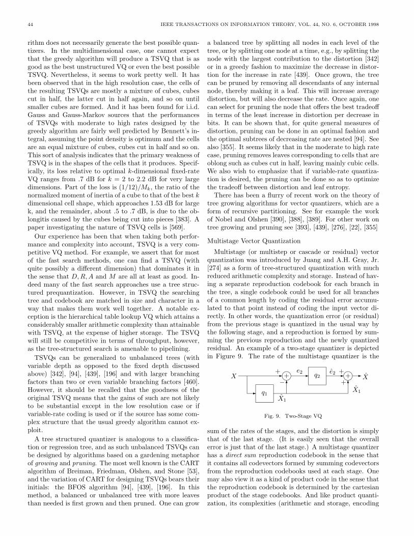
44 IEEE TRANSACTIONS ON INFORMATION THEORY, VOL. 44, NO. 6, OCTOBER 1998
rithm does not necessarily generate the best possible quan-tizers. In the multidimensional case, one cannot expectthat the greedy algorithm will produce a TSVQ that is asgood as the best unstructured VQ or even the best possibleTSVQ. Nevertheless, it seems to work pretty well. It hasbeen observed that in the high resolution case, the cells ofthe resulting TSVQs are mostly a mixture of cubes, cubescut in half, the latter cut in half again, and so on untilsmaller cubes are formed. And it has been found for i.i.d.Gauss and Gauss-Markov sources that the performancesof TSVQs with moderate to high rates designed by thegreedy algorithm are fairly well predicted by Bennett’s in-tegral, assuming the point density is optimum and the cellsare an equal mixture of cubes, cubes cut in half and so on.This sort of analysis indicates that the primary weakness ofTSVQ is in the shapes of the cells that it produces. Specif-ically, its loss relative to optimal k-dimensional fixed-rateVQ ranges from .7 dB for k = 2 to 2.2 dB for very largedimensions. Part of the loss is (1/12)/Mk, the ratio of thenormalized moment of inertia of a cube to that of the best kdimensional cell shape, which approaches 1.53 dB for largek, and the remainder, about .5 to .7 dB, is due to the ob-longitis caused by the cubes being cut into pieces [383]. Apaper investigating the nature of TSVQ cells is [569].
Our experience has been that when taking both perfor-mance and complexity into account, TSVQ is a very com-petitive VQ method. For example, we assert that for mostof the fast search methods, one can find a TSVQ (withquite possibly a different dimension) that dominates it inthe sense that D,R,A and M are all at least as good. In-deed many of the fast search approaches use a tree struc-tured prequantization. However, in TSVQ the searchingtree and codebook are matched in size and character in away that makes them work well together. A notable ex-ception is the hierarchical table lookup VQ which attains aconsiderably smaller arithmetic complexity than attainablewith TSVQ, at the expense of higher storage. The TSVQwill still be competitive in terms of throughput, however,as the tree-structured search is amenable to pipelining.
TSVQs can be generalized to unbalanced trees (withvariable depth as opposed to the fixed depth discussedabove) [342], [94], [439], [196] and with larger branchingfactors than two or even variable branching factors [460].However, it should be recalled that the goodness of theoriginal TSVQ means that the gains of such are not likelyto be substantial except in the low resolution case or ifvariable-rate coding is used or if the source has some com-plex structure that the usual greedy algorithm cannot ex-ploit.
A tree structured quantizer is analogous to a classifica-tion or regression tree, and as such unbalanced TSVQs canbe designed by algorithms based on a gardening metaphorof growing and pruning. The most well known is the CARTalgorithm of Breiman, Friedman, Olshen, and Stone [53],and the variation of CART for designing TSVQs bears theirinitials: the BFOS algorithm [94], [439], [196]. In thismethod, a balanced or unbalanced tree with more leavesthan needed is first grown and then pruned. One can grow
a balanced tree by splitting all nodes in each level of thetree, or by splitting one node at a time, e.g., by splitting thenode with the largest contribution to the distortion [342]or in a greedy fashion to maximize the decrease in distor-tion for the increase in rate [439]. Once grown, the treecan be pruned by removing all descendants of any internalnode, thereby making it a leaf. This will increase averagedistortion, but will also decrease the rate. Once again, onecan select for pruning the node that offers the best tradeoffin terms of the least increase in distortion per decrease inbits. It can be shown that, for quite general measures ofdistortion, pruning can be done in an optimal fashion andthe optimal subtrees of decreasing rate are nested [94]. Seealso [355]. It seems likely that in the moderate to high ratecase, pruning removes leaves corresponding to cells that areoblong such as cubes cut in half, leaving mainly cubic cells.We also wish to emphasize that if variable-rate quantiza-tion is desired, the pruning can be done so as to optimizethe tradeoff between distortion and leaf entropy.
There has been a flurry of recent work on the theory oftree growing algorithms for vector quantizers, which are aform of recursive partitioning. See for example the workof Nobel and Olshen [390], [388], [389]. For other work ontree growing and pruning see [393], [439], [276], [22], [355]
Multistage Vector Quantization
Multistage (or multistep or cascade or residual) vectorquantization was introduced by Juang and A.H. Gray, Jr.[274] as a form of tree-structured quantization with muchreduced arithmetic complexity and storage. Instead of hav-ing a separate reproduction codebook for each branch inthe tree, a single codebook could be used for all branchesof a common length by coding the residual error accumu-lated to that point instead of coding the input vector di-rectly. In other words, the quantization error (or residual)from the previous stage is quantized in the usual way bythe following stage, and a reproduction is formed by sum-ming the previous reproduction and the newly quantizedresidual. An example of a two-stage quantizer is depictedin Figure 9. The rate of the multistage quantizer is the
X - l++
−- q1
X1
6
-e2 q2 -e2 l++
+6X1
- X
Fig. 9. Two-Stage VQ
sum of the rates of the stages, and the distortion is simplythat of the last stage. (It is easily seen that the overallerror is just that of the last stage.) A multistage quantizerhas a direct sum reproduction codebook in the sense thatit contains all codevectors formed by summing codevectorsfrom the reproduction codebooks used at each stage. Onemay also view it as a kind of product code in the sense thatthe reproduction codebook is determined by the cartesianproduct of the stage codebooks. And like product quanti-zation, its complexities (arithmetic and storage, encoding
GRAY AND NEUHOFF: QUANTIZATION 45
and decoding) are the sum of those of the stage quantiz-ers plus a small amount for computing the residuals at theencoder or the sums at the decoder. In contrast a con-ventional single stage quantizer with the same rate anddimension has complexities equal to the product of thoseof the stage quantizers.
Since the total rate is the sum of the stage rates, a bitallocation problem arises. In two-stage quantization us-ing fixed-rate, unstructured, k-dimensional VQ’s in bothstages, it usually happens that choosing both stages to havethe same rate leads to the best performance vs. complexitytradeoff. In this case the complexities are approximatelythe square root of what they would be for a single stagequantizer.
Though we restrict attention here to the case where allstages are fixed-rate vector quantizers with the same di-mension, there is no reason why they need have the samedimension, have fixed rate, or have any similarity whatso-ever. In other words, multistage quantization can be used(and often is) with very different kinds of quantizers in itsstages (different dimensions and much different structures,e.g. DPCM or wavelet coding). For example, structuringthe stage quantizers leads to good performance and furthersubstantial reductions in complexity, e.g. [243], [79].
Of course, the multistage structuring leads to a subop-timal VQ for its given dimension. In particular the di-rect sum form of the codebook is not usually optimal, andthe greedy search algorithm described above, in which theresidual from one stage is quantized by the next, does notfind the closest codevector in the direct sum codebook.Moreover, the usual greedy design method, which uses aLloyd algorithm to design the first stage in the usual wayand then to design the second stage to minimize distortionwhen operating on the errors of the first, and so on, doesnot, in general, design an optimal multistage VQ, even forgreedy search. However, two-stage VQ’s designed in thisway work fairly well.
A high resolution analysis of two-stage VQ using Ben-nett’s integral on the second stage can be found in [311],[309]. In order to apply Bennett’s integral, it was necessaryto find the form of the probability density of the quanti-zation error produced by the first stage. This motivatedthe asymptotic error density analysis of vector quantiza-tion in [312], [379].
Multistage quantizers have been improved in a numberof ways. More sophisticated (than greedy) encoding al-gorithms can take advantage of the direct sum nature ofthe codebook to make optimal or nearly optimal searches,though with some (and sometimes a great deal of) in-creased complexity. And more sophisticated design algo-rithms (than the greedy one) can also have benefits [32],[177], [81], [31], [33]. Variable-rate multistage quantizershave been developed [243], [297], [298], [441], [296].
Another way of improving multistage VQ is to adapteach stage to the outcome of the previous. One suchscheme, introduced by Lee and Neuhoff [310], [309], wasmotivated by the observation that if the first stage quan-tizer has high rate, say R1, then by Gersho’s conjecture, the
first stage cells all have approximately the shape of Tk, thetesselating polytope with least normalized moment of in-ertia, and the source density is approximately constant onthem. This implies that the conditional distribution of theresidual given that the source vector lies in the ith cell dif-fers from that for the jth only by a scaling and rotation, be-cause cell Sj differs from Si by just a scaling and rotation.Therefore, if first-stage-dependent scaling and rotation aredone prior to second stage quantization, the conditionaldistribution of the residual will be the same for all cells,and the second stage can be designed for this distribution,rather than having to be a compromise, as is otherwise thecase in two-stage VQ. Moreover since this distribution isessentially uniform on a support region shaped like Tk, thesecond stage can itself be a uniform tesselation. The neteffect is a quantizer that inherits the optimal point den-sity of the first stage13 and the optimal cell shapes of thesecond. Therefore, in the high resolution case, this cell-conditioned two-stage VQ works essentially as well as anoptimal (single-stage) VQ, but with much less complexity.
Direct implementation of cell-conditioned two-stage VQ,requires the storing of a scale factor and a rotation foreach first stage cell, which operate on the first stage resid-ual before quantization by the second stage. Their in-verses are applied subsequently. However, since the firststage cells are so nearly spherical, the rotations gain only asmall amount, typically about 0.1 dB, and may be omitted.Moreover, since the best known lattice tesselations are soclose to the best known tesselations, one may use latticeVQ as the second stage, which further reduces complexity.Good schemes of this sort have even been developed forlow to moderate rates by Gibson [270], [271] and Pan andFischer [403], [404].
Cell-conditioned two-stage quantizers can be viewed ashaving a piecewise constant point density of the sort pro-posed earlier by Kuhlmann and Bucklew [302] as a meansof circumventing the fact that optimal vector quantizerscannot be implemented with companders. This approachwas further developed by Swaszek in [487].
Another scheme for adapting each stage to the previ-ous is called codebook sharing, as introduced by Chan andGersho [80], [82]. With this approach, each stage has afinite set of reproduction codebooks, one of which is usedto quantize the residual, depending on the sequence of out-comes from the previous stages. Thus each codebook isshared among some subset of the possible sequences of out-comes from the previous stages. This method lies betweenconventional multistage VQ in which each stage has onecodebook that is shared among all sequences of outcomesfrom previous stages, and TSVQ in which, in effect, a dif-ferent codebook is used for each sequence of outcomes fromthe previous stages. Chan and Gersho introduced a Lloyd-style iterative design algorithm for designing shared code-books; they showed that by controlling the number andrate of the codebooks one could optimize multistage VQwith a constraint on storage; and they used this method
13Since the second stage uniformly refines the first stage cells, theoverall point density is approximately that of the first stage.
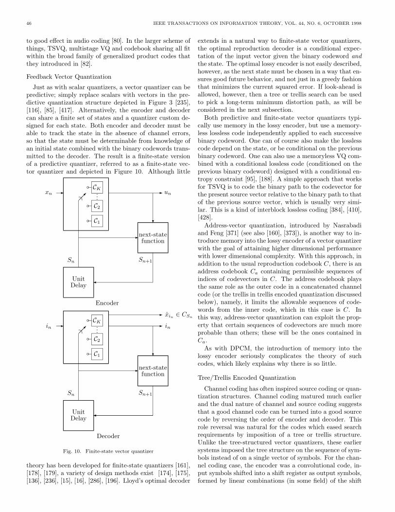
46 IEEE TRANSACTIONS ON INFORMATION THEORY, VOL. 44, NO. 6, OCTOBER 1998
to good effect in audio coding [80]. In the larger scheme ofthings, TSVQ, multistage VQ and codebook sharing all fitwithin the broad family of generalized product codes thatthey introduced in [82].
Feedback Vector Quantization
Just as with scalar quantizers, a vector quantizer can bepredictive; simply replace scalars with vectors in the pre-dictive quantization structure depicted in Figure 3 [235],[116], [85], [417]. Alternatively, the encoder and decodercan share a finite set of states and a quantizer custom de-signed for each state. Both encoder and decoder must beable to track the state in the absence of channel errors,so that the state must be determinable from knowledge ofan initial state combined with the binary codewords trans-mitted to the decoder. The result is a finite-state versionof a predictive quantizer, referred to as a finite-state vec-tor quantizer and depicted in Figure 10. Although little
UnitDelay
next-statefunction
-xn
Sn
-
Sn+1
�
- un
?
����C1
C2
...
CK
bbb
Encoder
UnitDelay
next-statefunction
-in
Sn
-
Sn+1
- xin ∈ CSn
��
- in
?
����C1
C2
...
CK
bbb
Decoder
Fig. 10. Finite-state vector quantizer
theory has been developed for finite-state quantizers [161],[178], [179], a variety of design methods exist [174], [175],[136], [236], [15], [16], [286], [196]. Lloyd’s optimal decoder
extends in a natural way to finite-state vector quantizers,the optimal reproduction decoder is a conditional expec-tation of the input vector given the binary codeword andthe state. The optimal lossy encoder is not easily described,however, as the next state must be chosen in a way that en-sures good future behavior, and not just in a greedy fashionthat minimizes the current squared error. If look-ahead isallowed, however, then a tree or trellis search can be usedto pick a long-term minimum distortion path, as will beconsidered in the next subsection.
Both predictive and finite-state vector quantizers typi-cally use memory in the lossy encoder, but use a memory-less lossless code independently applied to each successivebinary codeword. One can of course also make the losslesscode depend on the state, or be conditional on the previousbinary codeword. One can also use a memoryless VQ com-bined with a conditional lossless code (conditioned on theprevious binary codeword) designed with a conditional en-tropy constraint [95], [188]. A simple approach that worksfor TSVQ is to code the binary path to the codevector forthe present source vector relative to the binary path to thatof the previous source vector, which is usually very simi-lar. This is a kind of interblock lossless coding [384], [410],[428].
Address-vector quantization, introduced by Nasrabadiand Feng [371] (see also [160], [373]), is another way to in-troduce memory into the lossy encoder of a vector quantizerwith the goal of attaining higher dimensional performancewith lower dimensional complexity. With this approach, inaddition to the usual reproduction codebook C, there is anaddress codebook Ca containing permissible sequences ofindices of codevectors in C. The address codebook playsthe same role as the outer code in a concatenated channelcode (or the trellis in trellis encoded quantization discussedbelow), namely, it limits the allowable sequences of code-words from the inner code, which in this case is C. Inthis way, address-vector quantization can exploit the prop-erty that certain sequences of codevectors are much moreprobable than others; these will be the ones contained inCa.
As with DPCM, the introduction of memory into thelossy encoder seriously complicates the theory of suchcodes, which likely explains why there is so little.
Tree/Trellis Encoded Quantization
Channel coding has often inspired source coding or quan-tization structures. Channel coding matured much earlierand the dual nature of channel and source coding suggeststhat a good channel code can be turned into a good sourcecode by reversing the order of encoder and decoder. Thisrole reversal was natural for the codes which eased searchrequirements by imposition of a tree or trellis structure.Unlike the tree-structured vector quantizers, these earliersystems imposed the tree structure on the sequence of sym-bols instead of on a single vector of symbols. For the chan-nel coding case, the encoder was a convolutional code, in-put symbols shifted into a shift register as output symbols,formed by linear combinations (in some field) of the shift
GRAY AND NEUHOFF: QUANTIZATION 47
register contents, shifted out. Sequences of output sym-bols produced in this fashion could be depicted with a treestructure, where each node of the tree corresponded to thestate of the shift register (all but the final or oldest sym-bol) and the branches connecting nodes were determinedby the most recent symbol to enter the shift register andwere labeled by the corresponding output, the output sym-bol resulting if that branch is taken. The goal of a channeldecoder is to take such a sequence of tree branch labelsthat has been corrupted by noise, and find a minimumdistance valid sequence of branch labels. This could be ac-complished by a tree-search algorithm such as the Fano,stack, or M-algorithm. Since the shift register is finite, thetree becomes redundant and new nodes will correspond topreviously seen states so that the tree diagram becomes amerged tree or trellis, which can be searched by a dynamicprogramming algorithm, the Viterbi algorithm, cf. [173]. Inthe early 1970’s the algorithms for tree decoding channelcodes were inverted to form tree-encoding algorithms forsources by Jelinek, Anderson, and others [268], [269], [11],[132], [123], [10] Later trellis channel decoding algorithmswere modified to trellis-encoding algorithms for sources byViterbi and Omura [519]. While linear encoders sufficedfor channel coding, nonlinear decoders were required forthe source coding application, and a variety of design al-gorithms were developed for designing the decoder to pop-ulate the trellis searched by the encoder [319], [531], [481],[18], [40]. Observe that the reproduction decoder of a finite-state VQ can be used as the decoder in a trellis-encodingsystem, where the finite-state encoder is replaced by a min-imum distortion search of the decoder trellis implied by thefinite-state VQ decoder, which is an optimal encoding fora sequence of inputs.
Tree and trellis encoded quantizers can both be consid-ered as a VQ with large blocklength and a reproductioncodebook constrained to be the possible outputs of a non-linear filter or a finite-state quantizer or vector quantizerof smaller dimension. Both structures produce long code-words with a trellis structure, i.e., successive reproductionsymbols label the branches of a trellis and the encoder isjust a minimum distortion trellis search algorithm such asthe Viterbi algorithm.
Trellis Coded Quantization
Trellis coded quantization, both scalar and vector, im-proves upon traditional trellis encoded systems by label-ing the trellis branches with entire subcodebooks (or “sub-sets”) rather than with individual reproduction levels [345],[344], [166], [167], [522], [343], [478], [514]. The primarygain resulting is a reduction in encoder complexity for agiven level of performance. As the original trellis encod-ing systems were motivated by convolutional channel codeswith Viterbi decoders, trellis coded quantization was moti-vated by Ungerboeck’s enormously successful coded mod-ulation approach to channel coding for narrowband chan-nels [505], [506].
Recent combinations of TCQ to coding wavelet coeffi-cients [478] have yielded excellent performance in image
coding applications, winning the JPEG 2000 contest of1997 and thereby a position as a serious contender for thenew standard.
Gaussian Quantizers
Shannon [465] showed that a Gaussian i.i.d. sourcehad the worst rate-distortion function of any i.i.d. sourcewith the same variance, thereby showing that the Gaussiansource was an extremum in a source coding sense. It waslong assumed and eventually proved by Sakrison in 1975[456] that this provided a robust approach to quantizationin the sense there exist vector quantizers designed for thei.i.d. Gaussian source with a given average distortion whichwill provide no worse distortion when applied to any i.i.d.source with the same variance. This provided an approachto robust vector quantization, having a code that might notbe optimal for the actual source, but which would performno worse than it would on the Gaussian source for whichit was designed.
Sakrison extended the extremal properties of the ratedistortion functions to sources with memory [453], [454],[455] and Lapidoth [306] (1997) showed that a code de-signed for a Gaussian source would yield essentially thesame performance when applied to another process withthe same covariance structure.
These results are essentially Shannon theory and henceshould be viewed as primarily of interest for high-dimensional quantizers.
In a different approach towards using a Gaussian quan-tizer on an arbitrary source, Popat and Zeger (1992) tookadvantage of the central limit theorem and the knownstructure of an optimal scalar quantizer for a Gaussian ran-dom variable to code a general process by first filtering it toproduce an approximately Gaussian density, scalar quan-tizing the result, and then inverse filtering to recover theoriginal [419].
C. Robust Quantization
The Gaussian quantizers were described as being robustin a minimax average sense: a vector quantizer suitablydesigned for a Gaussian source will yield no worse averagedistortion for any source in the class of all sources withthe same second order properties. An alternative formula-tion of robust quantization is obtained if instead of dealingwith average distortion, as is done in most of this paper,one places a maximum distortion requirement on quan-tizer design. Here a quantizer is considered to be robustif it bounds the maximum distortion for a class of sources.Morris and Vandelinde (1974) [361] developed the theoryof robust quantization and provide conditions under whichthe uniform quantizer is optimum in this minimax sense.This can be viewed as a variation on epsilon entropy sincethe goal is to minimize the maximum distortion. Furtherresults along this line may be found in [37], [275], [491].Because these are minimax results aimed at scalar quanti-zation, these results apply to any rate or dimension.
48 IEEE TRANSACTIONS ON INFORMATION THEORY, VOL. 44, NO. 6, OCTOBER 1998
D. Universal Quantization
The minimax approaches provide one means of designinga fixed rate quantizer for a source with unknown or par-tially known statistics: a quantizer can be designed thatwill perform no worse than a fixed value of distortion for allsources in some collection. An alternative approach is to bemore greedy and try to design a code that yields nearly op-timal performance regardless of which source within somecollection is actually coded. This is the idea behind uni-versal quantization.
Universal quantization or universal source coding hadits origins in an approach to universal lossless compressiondeveloped by Rice and Plaunt [435], [436] and dubbed the“Rice machine.” Their idea was to have a lossless coderthat would work well for distinct sources by running mul-tiple lossless codes in parallel and choosing the one pro-ducing the fewest bits for a period of time, sending a smallamount of overhead to inform the decoder which code theencoder was using. The classic work on lossy universalsource codes was Ziv’s 1972 paper [577], which proved theexistence of fixed-rate universal lossy codes under certainassumptions on the source statistics and the source andcodebook alphabets. The multiple codebook idea was alsoused in 1974 [221] to extend the Shannon source codingtheorem to nonergodic stationary sources by using the er-godic decomposition to interpret a nonergodic source asa universal coding problem for a family of ergodic sources.The idea is easily described and provides one means of con-structing universal codes. Suppose that one has a collec-tion of k-dimensional codebooks Ck with 2kRk codevectors,k = 1, . . . ,K, each designed for a different type of localbehavior. For example, one might have different code-books in an image coder for edges, textures, and gradi-ents. The union codebook
⋃Kk=1 Ck then contains all the
codevectors in all of the codes, for a total of∑Kk=1 2kRk
codevectors. Thus, for example, if all of the subcodebooksCk have equal rate Rk = R, then the rate of the universalcode is R+ k−1 logK bits per symbol, which can be smallif the dimension k is moderately large. This does not meanthat it is necessary to use a large dimensional VQ, sincethe VQ can be a product VQ, e.g., for an image one couldhave k = 64 by coding each square of dimension 8×8 = 64using four applications of a VQ of dimension 4 × 4 = 16.If one had, say, 4 different codes, the resulting rate wouldbe R+ 2/64 = R+ 0.031, which would be a small increaseover the original rate if the original rate is, say, .25.
A universal code is in theory more complicated thanan ordinary code, but in practice it can mean codes withsmaller dimension might be more efficient since separatecodebooks can be used for distinct short term behavior.
Subsequently a variety of notions of fixed-rate uni-versal codes were considered and compared [382], andfixed-distortion codes with variable-rate were developed byMackenthun and Pursley [340] and Kieffer [277], [279].
As with the early development of block source codes,universal quantization during its early days in the 1970swas viewed as more of a method for developing the theory
than as a practical code design algorithm. The Rice ma-chine, however, proved the practicality and importance ofa simple multiple codebook scheme for handling compositesources.
These works all assumed the encoder and decoder to pos-sess copies of the codebooks being used. Zeger, Bist, andLinder [566] considered systems where the codebooks aredesigned at the encoder, but must be also coded and trans-mitted to the decoder, as is commonly done in codebookreplenishment [206].
A good review of the history of universal source cod-ing through the early 1990s may be found in Kieffer(1993) [283].
Better performance tradeoffs can be achieved by allow-ing both rate and distortion to vary, and in 1996 Chouet al. [92] formulated the universal coding problem as anentropy-constrained vector quantization problem for a fam-ily of sources and provided existence proofs and Lloyd-styledesign algorithms for the collection of codebooks subjectto a Lagrangian distortion measure, yielding a fixed rate-distortion slope optimization rather than fixed distortion orfixed rate. The clustering of codebooks was originally dueto Chou [90] in 1991. High resolution quantization theorywas used to study rates of convergence with blocklength tothe optimal performance, yielding results consistent withearlier convergence results developed by other means, e.g.,Linder et al. [321]. The fixed-slope universal quantizer ap-proach was further developed with other code structuresand design algorithms by Yang et al. [558].
A different approach which more closely resembles tradi-tional adaptive and codebook replenishment was developedby Zhang, Yang, Wei, and Liu [329], [575], [574]. Their ap-proach, dubbed “gold washing” did not involve training,but rather created and removed codevectors according tothe data received and an auxiliary random process in a waythat could be tracked by a decoder without side informa-tion.
E. Dithering
Dithered quantization was introduced by Roberts [442]in 1962 as a means of randomizing the effects of uniformquantization so as to minimize visual artifacts. It was fur-ther developed for images by Limb (1969) [317] and forspeech by Jayant and Rabiner (1972) [266]. Intuitively,the goal was to cause the reconstruction error to look morelike signal-independent additive white noise. It turns outthat for one type of dithering, this intuition is true. In adithered quantizer, instead of quantizing an input signalXn directly, one quantizes a signal Un = Xn + Wn, whereWn is a random process, independent of the signal Xn,called a dither process. The dither process is usually as-sumed to be i.i.d. . There are two approaches to dithering.Roberts considered subtractive dithering, where the finalreconstruction is formed as X = q(Xn + Wn) −Wn. Anobvious problem is the need for the decoder to possess acopy of the dither signal. Nonsubtractive dithering formsthe reproduction as X = q(Xn +Wn).
The principal theoretical property of nonsubtractive
GRAY AND NEUHOFF: QUANTIZATION 49
dithering was developed by Schuchman [461], who showedthat the quantizer error en = Xn − Xn = Xn − q(Xn +Wn) +Wn is uniformly distributed on (−∆/2,∆/2] and isindependent of the original input signal Xn if and only ifthe quantizer does not overload and the characteristic func-tion MW (ju) = E
[ejuW
]satisfies MW ( j2πl∆ ) = 0; l 6= 0.
Schuchman’s conditions are satisfied, for example, if thedither signal has a uniform probability density function on(−∆/2,∆/2]. It follows from the work of Jayant and Ra-biner [266] and Sripad and Snyder [477] (see also [216])that Schuchman’s condition implies that the sequence ofquantization errors {en} is independent. The case of uni-form dither remains by far the most widely studied in theliterature.
The subtractive dither result is nice mathematically be-cause it promises a well behaved quantization noise as wellas quantization error. It is impractical in many applica-tions, however, for two reasons. First, the receiver willusually not have a perfect analog link to the transmitter(or else the original signal could be sent in analog form)and hence a pseudo-random deterministic sequence mustbe used at both transmitter and receiver as proposed byRoberts. In this case, however, there will be no math-ematical guarantee that the quantization error and noisehave the properties which hold for genuinely random i.i.d.dither. Second, subtractive dither of a signal that indeedresembles a sample function of a memoryless random pro-cess is complicated to implement, requiring storage of thedither signal, high precision arithmetic, and perfect syn-chronization. As a result, it is of interest to study the be-havior of the quantization noise in a simple nonsubtractivedithered quantizer. Unlike subtractive dither, nonsubtrac-tive dither is not capable of making the reconstruction errorindependent of the input signal (although claims to the con-trary have been made in the literature). Proper choice ofdithering function can, however, make the conditional mo-ments of the reproduction error independent of the inputsignal. This can be practically important. For example, itcan make the perceived quantization noise energy constantas an input signal fades from high intensity to low inten-sity, where otherwise it can (and does) exhibit stronglysignal-dependent behavior. The properties of nonsubtrac-tive dither were originally developed in unpublished workby Wright [542] in 1979 and Brinton [54] in 1984 and subse-quently extended and refined with a variety of proofs [513],[512], [328], [227]. For any k = 1, 2, . . . necessary and suf-ficient conditions on the characteristic function MW areknown which ensure that the kth moment of the quantiza-tion noise εn = q(Xn +Wn)−Xn conditional on Xn doesnot depend on Xn. A sufficient condition is that the dithersignal consists of the sum of k independent uniformly dis-tributed random variables on [−∆/2,∆/2]. Unfortunatelythis conditional independence of moments comes at the ex-pense of a loss of fidelity. For example, if k = 2 then thequantizer noise power (the mean squared error) will be
E[ε2|X] = E[ε2] = E[W 2] +∆2
12.
This means that the power in the dither signal is directlyadded to that of the quantizer error in order to form theoverall mean squared error.
In addition to its role in whitening quantization noiseand making the noise or its moments independent of theinput, dithering has played a role in proofs of “universalquantization” results in information theory. For example,Ziv [578] showed that even without high resolution theory,uniform scalar quantization combined with dithering andvector lossless coding could yield performance within .75bits/symbol of the rate-distortion function. Extensions tolattice quantization and variations of this result have beendeveloped by Zamir and Feder [565]
F. Quantization for Noisy Channels
The separation theorem of information theory [464],[180] states that nearly optimal communication of an in-formation source over a noisy channel can be accomplishedby separately quantizing or source coding the source andchannel coding or error-control coding the resulting en-coded source for reliable transmission over a noisy chan-nel. Moreover, these two coding functions can be designedseparately, without knowledge of each other. The result isonly for point-to-point communications, however, and it isa limiting result in the sense that large block lengths andhence large complexity must be permitted. If one wishesto perform near the Shannon limit for moderate delay orblocklengths, or in multiuser situations, it is necessary toconsider joint source and channel codes, codes which jointlyconsider quantization and reliable communication. It maynot actually be necessary to combine the source and chan-nel codes, but simply to jointly design them. There are avariety of code structures and design methods that havebeen considered for this purpose, many of which involveissues of channel coding which are well beyond the focusof this paper. Here we mention only schemes which canbe viewed as quantizers which are modified for use on anoisy channel and not those schemes which involve explicitchannel codes. More general discussions can be found, e.g.,in [122].
One approach to designing quantizers for use on noisychannels is to replace the distortion measure with respectto which a quantizer is optimized by the expected distortionover the noisy channel. This simple modification of the dis-tortion measure allows the channel statistics to be includedin an optimal quantizer design formulation. Recently themethod has been referred to as “channel-optimized quan-tization,” where the quantization might be scalar, vector,or trellis.
This approach was introduced in 1969 by Kurtenbachand Wintz [304] for scalar quantizers. A Shannon sourcecoding theorem for trellis encoders using this distortionmeasure was proved in 1981 [135] and a Lloyd-style designalgorithm for such encoders provided in 1987 [19]. A Lloydalgorithm for vector quantizers using the modified distor-tion measure was introduced in 1984 by Kumazawa, Kasa-hara, and Namekawa [303] and further studied in [157],[152], [153]. The method has also been applied to tree-
50 IEEE TRANSACTIONS ON INFORMATION THEORY, VOL. 44, NO. 6, OCTOBER 1998
structured VQ [412]. It can be combined with a maxi-mum likelihood detector to further improve performanceand permit progressive transmission over a noisy chan-nel [411], [523]. Simulated annealing has also been usedto design such quantizers [140], [152], [354].
Another approach to joint-source and channel codingbased on a quantizer structure and not explicitly involv-ing typical channel coding techniques is to design a scalaror vector quantizer for the source without regard to thechannel, but then code the resulting indices in a waythat ensures that small (large) Hamming distance of thechannel codewords corresponds to small (large) distortionbetween the resulting reproduction codewords, essentiallyforcing the topology on the channel codewords to corre-spond to that of the resulting reproduction codewords.The codes that do this are often called index assignments.Several specific index assignment methods were consideredby Rydbeck and Sundberg [448]. DeMarca and Jayant in1987 [121] introduced an iterative search algorithm for de-signing index assignments for scalar quantizers, which wasextended to vector quantization by Zeger and Gersho [568],who dubbed the approach “pseudo-Gray” coding. Otherindex assignment algorithms include [210], [543], [287].For binary symmetric channels and certain special sourcesand quantizers, analytical results have been obtained [555],[556], [250], [501], [112], [351], [42], [232], [233], [352]. Forexample, it was shown by Crimmins et al. in 1969 [112]that the index assignment that minimizes mean squarederror for a uniform scalar quantizer used on a binary sym-metric channel is the natural binary assignment. However,this result remained relatively unknown until rederived andgeneralized in [351].
When source and channel codes are considered together,a key issue is the determination of the quantization rateto be used when the total of number of channel symbolsper source symbol is held fixed. For example, as quantiza-tion rate is increased, the quantization noise decreases, butchannel induced noise increases because the ability of thechannel code to protect the bits is reduced. Clearly, thereis an optimal choice of quantization rate. Another issue isthe determination of the rate at which overall distortion de-creases in an optimal system as the total number of channeluses per source symbol increases. These issues have beenaddressed in recent papers by Zeger and Manzella [570] andHochwald and Zeger [244], which use both exponential for-mulas produced by high resolution quantization theory andexponential bounds to channel coding error probability.
There are a variety of other approaches to joint sourceand channel coding, including the use of codes with a chan-nel encoder structure optimized for the source or with aspecial decoder matched to the source, using unequal er-ror protection for to better protect more important (lowerresolution) reproduction indexes, jointly optimized combi-nations of source and channel codes, and combinations ofchannel-optimized quantizers with source-optimized chan-nel codes, but we leave these to the literature as they in-volve a heavy dose of channel coding ideas.
G. Quantizing Noisy Sources
A parallel problem to quantizing for a noisy channel isquantizing for a noisy source. The problem can be seenas trying to compress a dirty source into a clean reproduc-tion, or as doing estimation of the original source basedon a quantized version of a noise-corrupted version. If theunderlying statistics are known or can be estimated by atraining sequence, then this can be treated as a quanti-zation problem with a modified distortion measure, wherenow the distortion between a noise corrupted observationY = y of an unseen original X and a reconstruction x basedon the encoded and decoded y is given as the conditionalexpectation E[d(X, x)|Y = y]. The usefulness of this modi-fied distortion for source coding noisy sources was first seenby Dobrushin and Tsybakov (1962) [134] and was used byFine (1965) [162] and Sakrison (1968) [452] to obtain infor-mation theoretic bounds an quantization and source cod-ing for noisy sources. Berger (1971) [46] explicitly used themodified distortion in his study of Shannon source codingtheorems for noise corrupted sources.
In 1970 Wolf and Ziv [537] used the modified distortionmeasure for a squared-error distortion to prove that theoptimal quantizer for the modified distortion could be de-composed into the cascade of a minimum mean-squarederror estimator followed by an optimal quantizer for theestimated original source. This result was subsequentlyextended to a more general class of distortion measures in-clude the input-weighted quadratic distortion of Ephraimand Gray [145], where a generalized Lloyd algorithm fordesign was presented.
Related results and approaches can be found in Witsen-hausen’s (1980) [535] treatment of rate distortion theorywith modified (or “indirect”) distortion measures, and inthe Occam filters of Natarajan (1995) [370].
H. Multiple Description Quantization
A topic closely related to quantization for noisy channelsis multiple description quantization. The problem is usu-ally formulated as a source coding or quantization problemover a network, but it is most easily described in terms ofpacket communications. In the simplest case, suppose thattwo packets of information, each of rate R, are transmit-ted to describe a reproduction of a single random vectorX. The encoder might receive one or the other packetor the two together and wishes to provide the best recon-struction possible for the bit rate it receives. This can beviewed as a network problem with one receiver seeing onlyone channel, another receiver seeing the second channel,and a third reciever seeing both channels, and the goal isthat each have an optimal reconstruction for the total re-ceived bitrate. Clearly one can do no better than havingeach packet alone result in in a reproduction with distor-tion near the Shannon distortion-rate function D(R) whilesimultaneously having the two packets together yield a re-production with distortion near D(2R), but this optimisticperformance is in general not possible. This problem wasfirst tackled in the information theory community in 1980by Wolf, Wyner, and Ziv [536] and Ozarow [401] who de-
GRAY AND NEUHOFF: QUANTIZATION 51
veloped achievable rate regions and lower bounds to perfor-mance. The results were extended by El Gamal and Cover(1982) [139], Ahlswede (1985) [6], and Zhang and Berger(1987) [573].
In 1993 Vaishampayan et al. used a Lloyd algo-rithm to actually design fixed rate [508] and entropy-constrained [509] scalar quantizers for the multiple descrip-tion problem. High resolution quantization ideas were usedto evaluate achievable performance in 1998 by Vaisham-payan and Batllo [510] and Linder, Zamir, and Zeger [324].An alternative approach to multiple description quantiza-tion using transform coding has also been considered, e.g.,in [38], [211].
I. Other Applications
We have not treated many interesting variations andapplications of quantization, several of which have beensuccessfully analyzed or designed using the tools describedhere. Examples which we would have included had time,space, and patience been more plentiful include mismatchresults for quantizers designed for one distribution and ap-plied to another, quantizers designed to provide inputs toclassification, detection, or estimation systems, quantiz-ers in multiuser systems such as simple networks, quan-tizers implicit in finite-precision arithmetic (the modernform of roundoff error), and quantization in noise-shapinganalog-to-digital and digital-to-analog converters such as∆Σ-modulators. Doubtless we have failed to mention afew, but this list suffices to demonstrate how rich the the-oretical and applied fields of quantization have become intheir half century of active development.
AcknowledgementsThe authors gratefully acknowledge the many help-
ful comments, corrections, and suggestions from colleagues,students, and reviewers. Of particular assistance were A.Gersho, B. Girod, N. Kashyap, T. Linder, N. Moayeri, P.Moo, Y. Shtarkov, S. Verdu, M. Vetterli, and K. Zeger..
References
[1] E. Abaya and G. L. Wise, “Some notes on optimal quantization,”Proc. Int’l Conf.Commun., vol. 2, pp. 30.7.1–30.7.5, June 1981.
[2] H. Abut, Vector Quantization, IEEE Reprint Collection, IEEEPress, Piscataway, NJ, 1990.
[3] J. P. Adoul, C. Collin and D. Dalle, “Block encoding and its ap-plication to data compression of PCM speech,” Proc. CanadianCommun. and EHV Conf., Montreal, pp. 145–148, 1978.
[4] J.-P. Adoul, J.-L. Debray, and D. Dalle, “Spectral distance mea-sure applied to the optimum design of DPCM coders with Lpredictors,” Proc. IEEE Intl. Conf. on Acoust. Speech and Sig-nal Processing (ICASSP), Denver, CO, pp. 512–515, 1980.
[5] E. Agrell and T. Eriksson, “Optimization of lattices for quanti-zation,” submitted for publication, 1996. This work also appearsin “Lattice-based quantization,” Part I., Report No. 17, Depart-ment of Information Theory, Chalmers University of Technology,Goteborg, Sweden, Oct. 1996.
[6] R. Ahlswede, “The rate-distortion region for multiple descrip-tions without excess rate,” IEEE Trans. Inform. Theory, vol. 31,pp. 721-726, Nov. 1985.
[7] N. Ahmed and T. Natarajan and K. Rao, “Discrete cosine trans-form,” IEEE Trans. Comput., vol. C–23, pp. 90—93, 1974.
[8] V. R. Algazi, “Useful approximation to optimum quantization,”IEEE Trans. Comm., vol. 14, pp. 297–301, June 1966.
[9] M. R. Anderberg, Cluster Analysis for Applications, AcademicPress, San Diego, 1973.
[10] J. B. Anderson and J. B. Bodie, “Tree encoding of speech,” IEEETrans. Inform. Theory, vol. 20, pp. 379–387, 1975.
[11] J. B. Anderson and F. Jelinek, “A 2-cycle algorithm for sourcecoding with a fidelity criterion,” IEEE Trans. Inform. Theory,vol. 19, pp. 77–92, Jan. 1973.
[12] M. Antonini, M. Barlaud, P. Mathieu, and I. Daubechies, “Im-age coding using vector quantization in the wavelet transformdomain,” in Proc. IEEE Intl. Conf. on Acoust. Speech and Sig-nal Processing (ICASSP), Albuquerque, pp. 2297–2300, April1990.
[13] M. Antonini, M. Barlaud, and P. Mathieu, “Image codingusing lattice vector quantization of wavelet coefficients,” inProc. IEEE Intl. Conf. on Acoust. Speech and Signal Processing(ICASSP), Vol.4 Toronto, Canada, pp. 2273–2276, May 1991.
[14] M. Antonini, M. Barlaud, P. Mathieu, and I. Daubechies, “Imagecoding using wavelet transform,” IEEE Trans. Image Process-ing, vol. 1, pp. 205–220, April 1992.
[15] R. Aravind and A. Gersho, “Low-rate image coding with finite-state vector quantization,” Proc. Intl. Conf.Acoustics, Speech,and Signal Processing (ICASSP, pp. 137–140, Tokyo, 1986.
[16] R. Aravind and A. Gersho, “Image compression based on vectorquantization with finite memory,” Optical Engineering, vol. 26,pp. 570–580, July 1987.
[17] D. S. Arnstein, “Quantization error in predictive coders,” IEEETrans. Comm., vol. 23, pp. 423–429, April 1975.
[18] E. Ayanoglu and R. M. Gray, “The design of predictive trelliswaveform coders using the generalized Lloyd algorithm,” IEEETrans. Comm., vol. 34, pp. 1073–1080, Nov. 1986.
[19] E. Ayanoglu and R. M. Gray, “The design of joint source andchannel trellis waveform coders,” IEEE Trans. Inform. Theory,pp. 855–865, Vol 33, Nov. 1987.
[20] R. L. Baker and R. M. Gray, “Image compression using non-adaptive spatial vector quantization,” Conf. Record of the Six-teenth Asilomar Conf. on Circuits Systems and Computers,Asilomar, CA, pp. 55–61, Nov. 1982.
[21] R. L. Baker and R. M. Gray, “Differential vector quantization ofachromatic imagery,” Proc. Int’l Picture Coding Symp., pp. 105-106, March 1983.
[22] M. Balakrishnan, W. A. Pearlman, and L. Lu, “Variable-ratetree-structured vector quantizers,” IEEE Trans. Inform. Theoryvol. 41, pp. 917–930, July 1995.
[23] A. S. Balamesh, “Block-constrained methods of fixed-rate en-tropy constrained quantization,” Ph.D.Dissertation, Universityof Michigan, Jan. 1993.
[24] A. S. Balamesh and D. L. Neuhoff, “New methods of fixed-rateentropy-coded quantization,” Proc. 1992 Conf. on Inform. Sci-ences and Systems, Princeton, NJ, pp. 665-670, March 1992.
[25] A. S. Balamesh and D. L. Neuhoff, Unpublished notes, 1992.[26] A. S. Balamesh and D. L. Neuhoff, “Block-constrained quantiza-
tion: asymptotic analysis,” DIMACS Series in Discrete Math.and Theoretical Computer Science, vol. 14, pp. 67-74, 1993.
52 IEEE TRANSACTIONS ON INFORMATION THEORY, VOL. 44, NO. 6, OCTOBER 1998
[27] A. S. Balamesh and D. L. Neuhoff, “A new fixed-rate quanti-zation scheme based on arithmetic coding,” Proc. IEEE Int’lSymp. Inform. Theory, San Antonio, p. 435, Jan. 1993.
[28] A. S. Balamesh and D. L. Neuhoff, “Block-constrained methodsof fixed-rate entropy-coded, scalar quantization,” submitted toIEEE Trans. Inform. Theory.
[29] G. B. Ball, “Data analysis in the social sciences: what aboutthe details?,” Proc. Fall Joint Computing Conf.,” pp. 533–559,Washington, D.C., Spartan Books, 1965.
[30] M. Barlaud, P. Sole, T. Gaidon, M. Antonini, and P. Mathieu,“Pyramidal lattice vector quantization for multiscale image cod-ing,” IEEE Trans. Image Processing, vol. 3, pp. 367–381, July1994.
[31] C. F. Barnes, “New multiple path search technique for residualvector quantizers,” Proc. Data Compression Conf., Snowbird,UT, pp. 42-51, 1994.
[32] C. F. Barnes and R. L. Frost, “Vector quantizers with direct sumcodebooks,” IEEE Trans. Inform. Theory, vol. 39, pp. 565–580,March 1993.
[33] C. F. Barnes, S. A. Rizvi, and N. M. Nasrabadi, “Advancesin residual vector quantization: a review,” IEEE Trans. ImageProcessing, vol. 5, pp. 226–262, Feb. 1996.
[34] C. W. Barnes, B. N. Tran, S. H. Leung,” “On the statistics offixed-point roundoff error,” IEEE Trans. Acoustics, Speech, andSignal Processing, vol. 3, pp. 595–606, June 1985.
[35] E. S. Barnes and N.J.A. Sloane, “The optimal lattice quantizerin three dimensions,” SIAM J. Alg. Discrete Methods, vol. 4,pp. 30–41, March 1983.
[36] P. Bartlett, T. Linder, and G. Lugosi, “The minimax distor-tion redundancy in empirical quantizer design,” Proc. IEEE Intl.Symp. on Inform. Theory, p. 511, Ulm, Germany, June 1997.(Submitted to the IEEE Trans. Inform. Theory.)
[37] W. G. Bath and V. D. Vandelinde, “Robust memoryless quan-tization for minimum signal distortion,” IEEE Trans. Inform.Theory, vol. 28, pp. 296–306, 1982.
[38] J.-C. Batllo and V. A. Vaishampayan, “Asymptotic performanceof multiple description codes,” IEEE Trans. Inform. Theory,vol. 43, pp. 703–707, March 1997.
[39] C. D. Bei and R. M. Gray, “An improvement of the minimumdistortion encoding algorithm for vector quantization,” IEEETrans. Comm., vol. 33, pp. 1132–1133, Oct. 1985.
[40] C. D. Bei and R. M. Gray, “Simulation of vector trellis encodingsystems,” IEEE Trans. Comm., vol. 34, pp. 214–218, March1986.
[41] P. Bello, R. Lincoln, and H. Gish, “Statistical delta modulation,”Proc. IEEE, vol. 55, pp. 308–319, March 1967.
[42] G. Ben-David and D. Malah, “On the performance of a vectorquantizer under channel errors,” Signal Proc. VI: Theories andApplications, Proc. EUSIPCO-92, pp. 1685–1688, 1992
[43] W. R. Bennett, “Spectra of quantized signals,” Bell Syst. Tech.J., vol. 27, pp. 446–472, July 1948.
[44] J. L. Bentley, “Multidimensional binary search trees used forassociative searching,” Comm. ACM, pp. 209-226, Sept. 1975.
[45] T. Berger, “Rate distortion theory for sources with abstract al-phabet and memory,” Inform. Contr., vol. 13, pp. 254–273, 1968.
[46] T. Berger, Rate Distortion Theory, Prentice-Hall,EnglewoodCliffs, NJ, 1971.
[47] T. Berger, “Optimum quantizers and permutation codes,” IEEETrans. Inform. Theory, vol. 18, pp. 759–765, November 1972.
[48] T. Berger, “Minimum entropy quantizers and permutationcodes,” IEEE Trans. Inform. Theory, vol. 28, pp. 149–157,March 1982.
[49] T. Berger, F. Jelinek, and J.K. Wolf, “Permutation codes forsources,” IEEE Trans. Inform. Theory, vol. 18, pp. 160–169,Jan. 1972.
[50] V. Bhaskaran and K. Konstantinides, Image and Video Com-pression Standards, Kluwer, Boston, 1995
[51] H. S. Black, “Pulse code modulation,” Bell Lab. Record., vol. 25,pp. 265–269, July 1947.
[52] R. E. Blahut, “Computation of channel capacity and rate-distortion functions,” IEEE Trans. Inform. Theory, vol. 18.pp. 460–473, July 1972.
[53] L. Breiman, J. H. Friedman, R. A. Olshen, and C. J. Stone,Classification and Regression Trees. Belmont, CA: Wadsworth,1984.
[54] L. K. Brinton, “Nonsubtractive Dither,” M.S. Thesis, ElectricalEngineering Department, University of Utah, Salt Lake City,Utah, Aug. 1984.
[55] J. D. Bruce, “On the optimum quantization of stationary sig-nals,” 1964 IEEE Int. Conv. Rec., Part 1, pp. 118-124, 1964.
[56] J. A. Bucklew, “Companding and random quantization in severaldimensions,” IEEE Trans. Inform. Theory, vol. 27, pp. 207–211,Mar. 1981.
[57] J. A. Bucklew, “A note on optimal multidimensional compan-ders,” IEEE Trans. Inform. Theory, vol. 29, p. 279, March 1983.
[58] J. A. Bucklew, “Two results on the asymptotic performance ofquantizers,” IEEE Trans. Inform. Theory, Vol. IT-30, pp. 341–348, March 1984.
[59] J. A. Bucklew, “A note on the absolute epsilon entropy,” IEEETrans. Inform. Theory, vol. 37, pp. 142–144, Jan. 1991.
[60] J. A. Bucklew and N. C. Gallagher, Jr., “A note on optimumquantization,” IEEE Trans. Inform. Theory, Vol. 25, pp. 365–366, May 1979.
[61] J. A. Bucklew and N. C. Gallagher, Jr., “Quantization schemesfor bivariate Gaussian random variables,” IEEE Trans. Inform.Theory, Vol. 25, pp. 537–543, September 1979.
[62] J. A. Bucklew and N. C. Gallagher, Jr., “Two-DimensionalQuantization of Bivariate Circularly Symmetric Densities,”IEEE Trans. Inform. Theory, vol. 25, pp. 667-671, Nov. 1979.
[63] J. A. Bucklew and N. C. Gallagher, Jr., “Some properties ofuniform step size quantizers,” IEEE Trans. Inform. Theory,Vol. IT-26, pp. 610–613, September 1980.
[64] J. A. Bucklew and G. L. Wise, “Multidimensional asymptoticquantization theory with rth power distortion measures, IEEETrans. Inform. Theory, vol. 28, pp. 239–247, March 1982.
[65] J. Buhmann and H. Kuhnel, “Vector quantization with complex-ity costs,” IEEE Trans. Inform. Theory, vol. 39, pp. 1133–1145,July 1988.
[66] P. J. Burt and E. H. Adelson, ‘The Laplacian pyramid as acompact image code,” IEEE Trans. Comm., vol. 31, pp. 532–540, April 1983.
[67] A. Buzo, R. M. Gray, A. H. Gray, Jr., and J. D. Markel, “Opti-mal quantizations of coefficient vectors in LPC speech,” 1978Joint Meeting of the Acoustical Society of America and theAcoustical Society of Japan, Honolulu, HI, Dec. 1978.
[68] A. Buzo, A. H. Gray, Jr., R. M. Gray and J. D. Markel, “Optimalquantizations of coefficient vectors in LPC speech,” Proc. IEEEIntl. Conf. on Acoust. Speech, and Signal Processing (ICASSP),pp. 52–55, Washington, D. C., April 1979.
[69] A. Buzo, A. H. Gray, Jr., R. M. Gray, and J. D. Markel, “Speechcoding based upon vector quantization,” IEEE Trans. Acoustics,Speech, and Signal Processing, vol. 28, pp. 562–574, Oct. 1980.
[70] S. Cambanis and N. Gerr, “A simple class of asymptotically opti-mal quantizers,” IEEE Trans. Inform. Theory, vol. 29, pp. 664-676, Sept. 1983.
[71] J. C. Candy and O. J. Benjamin, “The structure of quantiza-tion noise from Sigma-Delta modulation,” IEEE Trans. Comm.,vol. 29, pp. 1316–1323, Sept. 1981.
[72] J. Candy and G. Temes, Eds. Oversampling delta-sigma DataConverters, IEEE Press, 1991.
[73] R. M. Capocelli and A. DeSantis, “Variations on a theme by Gal-lager,” pp. 181–213, Image and Text Compression, J. A. Storer,ed., Kluwer, Boston, 1992.
[74] J. R. Caprio, N. Westin, and J. Esposito, “Optimum quanti-zation for minimum distortion,” Proc. of the Intl TelemeteringConf., pp. 315–323, 1978.
[75] N. Chaddha, M. Vishwanath and P. A. Chou, “Hierarchicalvector quantization of perceptually weighted block transforms,”Proc. Compression Conf., Snowbird, UT, pp. 3–12, IEEE Com-puter Society Press, 1995.
[76] D. L. Chaffee, “Applications of rate distortion theory to thebandwidth compression,” Ph.D. Dissertation, Electrical Engi-neering Department, Univ. of California, Los Angeles, 1975.
[77] D. L. Chaffee and J. K. Omura, “A very low rate voice com-pression system,” Abstracts of Papers of the IEEE Int’l Symp.Inform. Theory, Oct. 1974.
[78] C.-K. Chan and L.-M. Po, “A complexity reduction techniquefor image vector quantization,” IEEE Trans. Image Processing,vol. 1, pp. 312-321, July 1992.
[79] W.-Y. Chan and A. Gersho, “High fidelity audio transformcoding with vector quantization,” Proc. IEEE Intl. Conf. onAcoust., Speech, and Signal Processing (ICASSP) Albuquerque,New Mexico, vol. 2, pp. 1109-1112, April, 1990.
[80] W.-Y. Chan and A. Gersho, “Constrained-storage vector quan-tization in high fidelity audio transform coding,” Proc. IEEEICASSP, Toronto, pp. 3597-3600, May 1991.
GRAY AND NEUHOFF: QUANTIZATION 53
[81] W.-Y. Chan and A. Gersho, “Enhanced multistage vector quan-tization by joint codebook design,” IEEE Trans. Commun.,vol. 40, pp. 1693–1697, Nov. 1992.
[82] W.-Y. Chan and A. Gersho, “Generalized product code vectorquantization: a family of efficient techniques for signal compres-sion,” Digital Signal Processing, vol. 4, pp. 95-126, 1994.
[83] W.-Y. Chan, S. Gupta, and A. Gersho, “Enhanced multistagevector quantization by joint codebook design,” IEEE Trans.Comm., vol. 40, pp. 1693–1697, Nov. 1992.
[84] Y.-H. Chan and W. Siu, “In search of the optimal searchingsequence for VQ encoding,” IEEE Trans. Commun., vol. 43,pp. 2891-2893, Dec. 1995.
[85] P. C. Chang and R. M. Gray, “Gradient algorithms for designingpredictive vector quantizers,” IEEE Trans. Acoustics, Speech,and Signal Processing vol. 34, pp. 679–690, Aug. 1986.
[86] P. C. Chang, J. May, and R. M. Gray, “Hierarchical vector quan-tizers with table-lookup encoders,” Proc. 1985 IEEE Int’l Conf.Comm., vol. 3, pp. 1452–1455, June 1985.
[87] D. T. S. Chen, “On two or more dimensional optimum quantiz-ers,” Proc. IEEE Intl. Conf. Acoust., Speech, and Signal Pro-cessing (ICASSP), pp. 640–643, Hartford,CT, 1977.
[88] D.-Y. Cheng, A. Gersho, B. Ramamurthi, and Y. Shoham, “FastSearch Algorithms for Vector Quantization and Pattern Match-ing,” Proc. IEEE Intl. Conf. on Acoust., Speech, and SignalProcessing (ICASSP), San Diego, pp. 911.1–911.4, March 1984.
[89] D.-Y. Cheng and A. Gersho, “A fast codebook search algorithmfor nearest-neighbor pattern matching,” Proc. IEEE Intl. Conf.on Acoust., Speech, and Signal Processing (ICASSP), Tokyo,vol. 1, pp. 265-268, April 1986.
[90] P. A. Chou, “Code clustering for weighted universal VQ andother applications,” Proc. IEEE Int’l Symp.Inform. Theory, p.253, Budapest, Hungary, 1991.
[91] P. A. Chou, “The distortion of vector quantizers trained on nvectors decreases to the optimum as Op(1/n),” Proc. IEEE Int’lSymp. Inform. Theory, Trondheim, Norway, 1994.
[92] P. A. Chou, M. Effros, and R. M. Gray. “A vector quantizationapproach to universal noiseless coding and quantization,” IEEETrans. Inform. Theory, vol. 42, pp. 1109–1138, July 1996.
[93] P. A. Chou and T. Lookabaugh and R. M. Gray, “Entropy-Constrained Vector Quantization,” IEEE Trans. Acoustics,Speech, and Signal Processing vol. 37, pp. 31–42, Jan. 1989.
[94] P. A. Chou and T. Lookabaugh and R. M. Gray, “Optimal prun-ing with applications to tree-structured source coding and mod-eling,” IEEE Trans. Inform. Theory, vol. 35, pp. 299–315, Mar.1989
[95] P. A. Chou and T. Lookabaugh, “Conditional entropy-constrained vector quantization of linear predictive coefficients,”pp. 187–200, Proc. Intl. Conf. on Acoustics, Speech, and SignalProcessing, 1990.
[96] J. Chow and T. Berger, “Failure of successive refinement forsymmetric Gaussian mixtures,” IEEE Trans. Inform. Theory,vol. 43, pp. 350-352, Jan. 1957.
[97] T. A. C. M. Claasen and A. Jongepier, “Model for the powerspectral density of quantization noise,” IEEE Trans. Acoustics,Speech, and Signal Processing, vol. 29, pp. 914–917, Aug. 1981.
[98] R. J. Clarke, Transform Coding of Images, Academic Press, Or-landa, FL, 1985.
[99] A. G. Clavier, P. F. Panter, and D. D. Grieg, “Distortionin a Pulse Count Modulation System,” AIEE Trans., vol. 66,pp. 989–1005, 1947.
[100] A. G. Clavier, P. F. Panter, and D. D. Grieg, “PCM DistortionAnalysis,” Electrical Engineering, pp. 1110–1122, Nov. 1947.
[101] D. Cohn, E. Riskin, and R. Ladner, “Theory and practice ofvector quantizers trained on small training sets,” IEEE Trans.Pattern Analysis and Machine Intelligence, vol. 16, pp. 54–65,Jan. 1994.
[102] R. R. Coifman and M. V. Wickerhauser. “Entropy-based algo-rithms for best basis selection,” IEEE Trans. Inform. Theory,vol. 38, pp. 713–718, March 1992.
[103] J. H. Conway and N. J. A. Sloane, “Voronoi regions of lat-tices,second moments of polytopes,and quantization,” IEEETrans. Inform. Theory, vol. 28, pp. 211–226, March 1982
[104] J. H. Conway and N. J. A. Sloane, “Fast quantizing and decod-ing algorithms for lattice quantizers and codes,” IEEE Trans.Inform. Theory, vol. 28, pp. 227–232, March 1982.
[105] J. H. Conway and N. J. A. Sloane, “A fast encoding methodfor lattice codes and quantizers, IEEE Trans. Inform. Theory,Vol 29, pp. 820–824, Nov. 1983.
[106] J. H. Conway and N. J. A. Sloane, Sphere Packings,Latticesand Groups, Springer-Verlag, New York, 1988.
[107] P. C. Cosman, R. M. Gray, and M. Vetterli, “Vector quanti-zation of image subbands: A survey,” IEEE Trans. Image Pro-cessing, Vol.5, pp. 202-25. February, 1996.
[108] P. C. Cosman, K. O. Perlmutter, S. M. Perlmutter, R. M.Gray, and R. A. Olshen, “Training sequence size and vectorquantizer performance,” Proc. Twenty-Fifth Annual AsilomarConverence on Signals, Systems, and Computers, Pacific Grove,Calif., pp. 434–438. Nov. 1991.
[109] P. C. Cosman, S. M. Perlmutter, and K. O. Perlmutter,“Tree-structured vector quantization with significance map forwavelet image coding,” Proc. 1995 IEEE Data CompressionConf. (DCC), J. A. Storer and M. Cohn, Eds., Snowbird, Utah,IEEE Computer Society Press, March 1995, .
[110] T .M. Cover and J. A. Thomas, Elements of Information The-ory, Wiley, Chichester, UK, 1991.
[111] D. R. Cox, “Note on grouping,” J. Amer. Statistical Assoc.,vol. 52, 543–547, 1957.
[112] T.R . Crimmins, H. M. Horwitz, C. J. Palermo, and R. V.Palermo, “Minimization of Mean-Squared Error for Data Trans-mitted via Group Codes,” IEEE Trans. Inform. Theory, vol. 15,pp. 72–78, Jan. 1969.
[113] R. E. Crochiere, S. M. Webber, and J. K. L. Flanagan. “Digitalcoding of speech in sub-bands,” Bell Syst. Tech. J., vol. 55,pp. 1069–1086, Oct. 1976.
[114] I. Csiszar, “Generalized entropy and quantization problems,”Proc. Sixth Prague Conf., pp. 159–174, 1973.
[115] I. Csiszar and J. Korner, Information Theory: Coding Theo-rems for Discrete Memoryless Systems, Academic Press, NewYork, 1981.
[116] V. Cuperman and A. Gersho, “Vector predictive coding ofspeech at 16 Kb/s,” IEEE Trans. Comm., vol. 33, pp. 685–696,July 1985.
[117] C. C. Cutler, “Differential quantization of communication sig-nals,” U.S. Patent 2 605 361, July 29, 1952.
[118] T. Dalenius, “The problem of optimum stratification,” Skandi-navisk Aktuarietidskrift, vol. 33, pp. 201–213, 1950.
[119] T. Dalenius and M. Gurney, “The problem of optimum stratifi-cation II,” Skandinavisk Aktuarietidskrift, vol. 34, pp. 203–213,1951.
[120] E. M. Deloraine and A. H. Reeves, “The 25th anniversary ofpulse code modulation,” IEEE Spectrum, pp. 56-64, May 1965.
[121] J. R.B. DeMarca and N. S. Jayant, “An algorithm for assigningbinary indices to the codevectors of multidimensional quantiz-ers,” Proc. IEEE Int’l Conf. Commun., pp. 1128–1132, June1987.
[122] N. Demir and K. Sayood “Joint source/channel coding for vari-able length codes,” Proc. 1998 IEEE Data Compression Conf.,J. A. Storer, M. Cohn, Eds., Computer Society Press, pp. 139–148, March 1998.
[123] C. R. Davis and M. E. Hellman, “On tree coding with a fidelitycriterion,” IEEE Trans. Inform. Theory, vol. 21, pp. 373–378,July 1975.
[124] L. D. Davission, “Information rates for data compression,”IEEE WESCON, Session 8, Paper 1, 1968.
[125] L. D. Davisson and R. M. Gray, Eds., Data Compression,vol. 14, in Benchmark Papers in Electrical Engineering andComputer Science, Dowden, Hutchinson and Ross, Stroudsburg,Penn., 1976.
[126] L. D. Davisson, A. Leon-Garcia and D. L. Neuhoff, “New re-sults on coding of stationary nonergodic sources,” IEEE Trans.Inform. Theory, vol. 25, pp. 137-144, Mar. 1979.
[127] L. D. Davisson and M. B. Pursley, “A direct proof of the cod-ing theorem for discrete sources with memory,” IEEE Trans.Inform. Theory, vol. 21, pp. 301–310, May 1975.
[128] F. DeJager, “Delta modulation, a method of PCM transmissionusing a one-unit code,” Philips Research Rept., vol. 7, 1952.
[129] B. Derjavitch, E. M. Deloraine and V. Mierlo, French PatentNo. 932, 140, Aug. 1946.
[130] R. A. DeVore, B. Jawerth, and B. Lucier, “Image compressionthrough wavelet transform coding,” IEEE Trans. Inform. The-ory, vol. 38, pp. 719–746, March 1992.
[131] L. Devroye, L. Gyorfi, and G. Lugosi, A Probabilistic Theoryof Pattern Recognition, Springer, New York, 1996.
[132] R. J. Dick, T. Berger, and F. Jelinek, “Tree encoding of Gaus-sian sources,” IEEE Trans. Inform. Theory, vol. 20, pp. 332–336,May 1974.
54 IEEE TRANSACTIONS ON INFORMATION THEORY, VOL. 44, NO. 6, OCTOBER 1998
[133] E. Diday and J. C. Simon, “Clustering analysis,” in DigitalPattern Recognition, K. S. Fu, Ed. Springer-Verlag, NY, 1976.
[134] R. L. Dobrushin and B. S. Tsybakov, “Information transmis-sion with additional noise,” IRE Trans. Inform. Theory, vol.IT-18, pp. S293-S304, 1962.
[135] J. G. Dunham and R. M. Gray, “Joint source and noisy channeltrellis encoding,” IEEE Trans. Inform. Theory, vol. 27, pp. 516–519, July 1981.
[136] M. Ostendorf Dunham and R. M. Gray, “An algorithm for thedesign of labeled-transition finite-state vector quantizers,” IEEETrans. Comm., vol. 33, pp. 83–89, Jan. 1985.
[137] J.G. Dunn, “The performance of a class of n dimensionalquantizers for a Gaussian source, Proc. Columbia Symp. SignalTransmission Processing, Columbia Univ., NY, pp. 76-81, 1965.Reprinted in Data Compression, L. D. Davisson and R. M. Gray,Ed., Benchmark Papers in Electrical Engineering and ComputerScience, vol. 14, Dowden, Hutchinson and Ross, Stroudsberg,PA, 1975.
[138] M. Effros, P.A. Chou, and R. M .Gray, “Variable–rate sourcecoding theorems for stationary nonergodic sources,” IEEETrans. Inform. Theory, Volume 40, No. 6, pp. 1920 – 1925,November 1994.
[139] A. E. El Gamal and T. M. Cover, “Achievable rates for multipledescriptions,” IEEE Trans. Inform. Theory, vol. 28, pp. 851–857, November 1982.
[140] A. E. El Gamal, L. A. Hemachandra, I. Shperling, and V. K.Wei, “Using simulated annealing to design good codes,” IEEETrans. Inform. Theory, vol. 33, pp. 116–123, Jan. 1987.
[141] P. Elias, “Predictive coding,” Ph.D. Dissertation, Harvard Uni-versity, Cambridge, MA, 1950.
[142] P. Elias, “Predictive coding I and II,” IRE Trans. Inform. The-ory, vol. 1, pp. 16–33, March 1955.
[143] P. Elias, “Bounds on performance of optimum quantizers,”IEEE Trans. Inform. Theory, vol. 16, pp. 172–184, March 1970.
[144] P. Elias, “Bounds and asymptotes for the performance of mul-tivariate quantizers,” Annals of Mathematical Statistics, vol. 41,No. 4 pp. 1249–1259, 1970.
[145] Y. Ephraim and R. M. Gray, “A unified approach for encodingclean and noisy sources by means of waveform and autoregres-sive vector quantization,” IEEE Trans. Inform. Theory, Vol. 34,pp. 826-834, July 1988.
[146] W. H. Equitz, “A new vector quantization clustering algo-rithm,” IEEE Trans. Acoustics, Speech, and Signal Processing,vol. 37, pp. 1568–1575, Oct. 1989.
[147] W. Equitz and T. Cover, “Successive refinement of informa-tion,” IEEE Trans. Inform. Theory, vol. 37, pp. 269-275, Mar.1991.
[148] T. Ericson, “A result on delay-less information transmission,”Abstracts of the IEEE Int. Symp. Inform. Theory, Grignano,Italy, June, 1979.
[149] T. Eriksson and E. Agrell, “Lattice-based quantization,Part II,” Report No. 18, Department of Information Theory,Chalmers University of Technology, Goteborg, Sweden, Oct.1996.
[150] A. M. Eskicioglu and P. S. Fisher, “Image Quality Measuresand Their Performance,” IEEE Trans. Comm., Vol 43, pp. 2959–2965, December 1995.
[151] M. Vedat Eyuboglu and G. David Forney, Jr., “Lattice andtrellis quantization with lattice- and trellis-bounded codebooks-High-rate theory for memoryless sources,” IEEE Trans. Inform.Theory, Vol.39, pp. 46–59, Jan. 1993.
[152] N. Farvardin, “A study of vector quantization for noisy chan-nels,” IEEE Trans. Inform. Theory, vol. 36, pp. 799–809, July1990.
[153] N. Farvardin, “On the performance and complexity of channeloptimized vector quantizers,” in Speech Recognition and Coding:New Advances and Trends, pp. 699–704, Springer, Berlin, 1995.
[154] N. Farvardin and F. Y. Lin, “Performance of entropy-constrained block transform quantizers,” IEEE Trans. Inform.Theory, vol. 37, pp. 1433–1439, September 1991.
[155] N. Farvardin and J. W. Modestino, “Optimal quantizer perfor-mance for a class of non-Gaussian memoryless sources,” IEEETrans. Inform. Theory, vol. 30, pp. 485–497, May 1984.
[156] N. Farvardin and J. W. Modestino, “Rate-distortion per-formance of DPCM schemes,” IEEE Trans. Inform. Theory,vol. 31, pp. 402–418, May 1985.
[157] N. Farvardin and V. Vaishampayan, “Optimal quantizer designfor noisy channels: An approach to combined source-channel
coding,” IEEE Trans. Inform. Theory, vol. 33, pp. 827–838,November 1987.
[158] L. Fejes Toth, Lagerungen in der Ebene, auf der Kugel und imRaum, Springer Verlag, Berlin, 1953.
[159] L. Fejes Toth, “Sur la representation d’une population infiniepar un nombre fini d’elements,” Acta Math. Acad. Sci. Hung.,vol. 10, pp. 76-81, 1959.
[160] Y. S. Feng and N. M. Nasrabadi, “Dynamic address-vectorquantisation of RGB colour images,” IEE Proc., Part I, Com-mun. Speech Vision, vol. 138, pp. 225-231, Aug. 1991.
[161] T. L. Fine, “Properties of an Optimal Digital System and Ap-plications,” IEEE Trans. Inform. Theory, vol. 10, pp. 287–296,Oct. 1964.
[162] T. Fine, “Optimum mean-square quantization of a noisy input,”IEEE Trans. Inform. Theory, vol. IT-11, pp. 293-294, Apr. 1965.
[163] T. L. Fine, “The response of a particular nonlinear system withfeedback to each of two random processes,” IEEE Trans. Inform.Theory, vol. 14, pp. 255-264, Mar. 1968.
[164] T. R. Fischer “A pyramid vector quantizer,” IEEE Trans. In-form. Theory, vol. 32, pp. 568–583, July 1986.
[165] T. R. Fischer “Geometric source coding and vector quantiza-tion,” IEEE Trans. Inform. Theory, vol. 35, pp. 137–145, July1989.
[166] T. R. Fischer, M. W. Marcellin, and M. Wang, “Trellis-codedvector quantization,” IEEE Trans. Inform. Theory, vol. 37,pp. 1551-1566, November 1991.
[167] T. R. Fischer and M. Wang, “Entropy-constrained trellis-codedquantization,” IEEE Trans. Inform. Theory, vol. 38, pp. 415–426, March 1992.
[168] S. Fix, “Rate distortion functions for continuous alphabet mem-oryless sources,” Ph.D. Dissertation, University of Michigan,1977.
[169] J. K. Flanagan, D. R. Morrell, R. L. Frost, C.J. Read, and B. E.Nelson, “Vector quantization codebook Generation using simu-lated annealing,” pp. 1759–1762, Proc. Intl. Conf. on Acoustics,Speech, and Signal Processing, Glasgow, Scotland, May 1989.
[170] P. Fleischer, “Sufficient conditions for achieving minimum dis-tortion in a quantizer,” IEEE Int. Conv. Rec., pp. 104–111, 1964.
[171] B. A. Flury “Principal points,” Biometrika, vol. 77, No. 1,pp. 31–41, 1990.
[172] E. Forgey, “Cluster analysis of multivariate data: efficiency vs.interpretability of classification,” Biometrics, vol. 21, pp. 768,1965. (Abstract)
[173] G. D. Forney, Jr., “The Viterbi Algorithm,” Proc. IEEE,vol. 61, pp. 268–278, March 1973.
[174] J. Foster and R. M. Gray, “Finite-state vector quantization,”Abstracts of the 1982 IEEE Int’l Symp. Inform. Theory, LesArcs France, June 1982.
[175] J. Foster, R. M. Gray, and M. Ostendorf Dunham, “Finite-statevector quantization for waveform coding,” IEEE Trans. Inform.Theory, vol. 31, pp. 348–359, May 1985.
[176] J. H. Friedman, F. Baskett and L. J. Shustek, “An algorithmfor finding nearest neighbors,” IEEE Trans. Computers, vol. 24,pp. 1000-1006, Oct. 1975.
[177] R. L. Frost, C. F. Barnes, and F. Xu, “Design and performanceof residual quantizers,” in Proc. Data Compression Conf., J. A.Storer and J. H. Reif, Eds., IEEE Computer Society Press, Snow-bird, Utah, pp. 129–138, April 1991.
[178] N. T. Gaarder and D. Slepian, “On optimal finite-state digitaltransmission systems,” IEEE Trans. Inform. Theory, vol. 28,pp. 167–186, March 1982.
[179] G. Gabor and Z. Gyorfi, “Recursive Source Coding,” Springer-Verlag, New York, 1986.
[180] R. G. Gallager, Information Theory and Reliable Communica-tion, Wiley, NY, 1968.
[181] R. G. Gallager ”Variations on a theme by Huffman,” IEEETrans. Inform. Theory, vol. 24, pp. 668-674, Nov. 1978.
[182] N. C. Gallagher, Jr., “Discrete Spectral Phase Coding,” IEEETrans. Inform. Theory, vol. 22, pp. 622-624, Sept. 1976.
[183] N. C. Gallagher, Jr., “Quantizing Schemes for the DiscreteFourier Transform of a Random Time-Series,” IEEE Trans. In-form. Theory, vol. 24, pp. 156-163, March 1978.
[184] N. C. Gallagher and J. A. Bucklew, “Properties of minimummean squared error block quantizers,” IEEE Trans. Inform.Theory, vol. 28, pp. 105-107, Jan. 1982.
[185] Z. Gao, F. Chen, B. Belzer, and J. Villasenor, “A comparison ofthe Z, E8, and Leech lattices for image subband quantization,”in Proc.1995 IEEE Data Compression Conf., pp. 312–321, J. A.
GRAY AND NEUHOFF: QUANTIZATION 55
Storer and M. Cohn, Eds., IEEE Computer Society Press, Snow-bird, Utah, March 1995.
[186] W. R. Gardner and B. D. Rao, “Theoretical Analysis of theHigh-Rate Vector Quantization of LPC Parameters,” IEEETrans. Speech and Audio Processing, Vol 3, pp. 367-381, Septem-ber 1995.
[187] M. Garey and D. S. Johnson and H. S. Witsenhausen, “Thecomplexity of the generalized Lloyd-Max problem,” IEEE Trans.Inform. Theory, vol. 28, pp. 255–266, March 1982.
[188] D. P. de Garrido, L. Lu, and W. A. Pearlman, “Conditionalentropy-constrained vector quantization of frame difference sub-band signals,” Proc. IEEE Int’l Conf. Image Proc. Austin, Part1 (of 3), pp. 745-749, 1994.
[189] N. L. Gerr and S. Cambanis, “Analysis of delayed delta modu-lation,” IEEE Trans. Inform. Theory, vol. 32, pp. 496-512, July1986.
[190] N. L. Gerr and S. Cambanis, “Analysis of adaptive differen-tial PCM of a stationary Gauss-Markov input,” IEEE Trans.Inform. Theory, vol. 3e, pp. 350-359, May 1987.
[191] A. Gersho, “Stochastic stability of delta modulation,” BellSyst. Tech. J., vol. 51, pp. 821-841, April 1972.
[192] A. Gersho, “Principles of Quantization,” IEEE Trans. CircuitsSyst, vol. 25, pp. 427–436, July 1978.
[193] A. Gersho, “Asymptotically optimal block quantization,” IEEETrans. Inform. Theory., vol. 25, pp. 373–380, July 1979.
[194] A. Gersho, “Optimal Nonlinear Interpolative Vector Quantiza-tion,” IEEE Trans. Commun. Vol.38, pp. 1285–1287, Sep. 1990.
[195] A. Gersho and V. Cuperman, “Vector Quantization: A pattern-matching technique for speech coding,” IEEE Commun. Maga-zine, vol. 21, pp. 15–21, Dec. 1983.
[196] A. Gersho and R. M. Gray, Vector Quantization and SignalCompression, Kluwer Academic Publishers, Boston, 1992.
[197] A. Gersho and B. Ramamurthi, “Image coding using vectorquantization,” Proc. Intl. Conf. on Acoust. Speech, and SignalProcessing, vol. 1, pp. 428–431, Paris, April 1982.
[198] J. D. Gibson, “Adaptive prediction in speech differential en-coding systems,” Proc. IEEE, vol. 68, pp. 488–525, April 1980.
[199] J. D. Gibson and K. Sayood, “Lattice quantization,” Advancesin Electronics and Electron Phys., vol. 72, pp. 259–330, 1988.
[200] N. Gilchrist and C. Grewin, Collected papers on digital audiobit-rate reduction, Audio Engineering Society, New York, 1996.
[201] B. Girod, “Rate-constrained Motion Estimation”, in VisualCommun. and Image Processing VCIP’94, A.K.Katsaggelos(ed.), Proc. SPIE vol. 2308, pp. 1026-1034, September 1994.
[202] B. Girod, R. M. Gray, J. Kovacevic. and M. Vetterli. “Im-age and Video Coding,” part of “The past, present, and futureof image and multidimensional signal processing,” edited by R.Chellappa, B. Girod, D.C. Munson, Jr., A. M. Telkap, and M.Vetterli, Signal Proc. Magazine, pp. 40–46, March 1998.
[203] H. Gish “Optimum quantization of random sequences,” Ph.D.Dissertation, Harvard University, March 1967.
[204] H. Gish and J. N. Pierce, “Asymptotically efficient quantizing,”IEEE Trans. Inform. Theory, vol. 14, pp. 676–683, Sep. 1968.
[205] T. J. Goblick and J. L. Holsinger, “Analog source digitization:A comparison of theory and practice,” IEEE Trans. Inform.Theory, vol. 13, pp. 323–326, April 1967.
[206] M. Goldberg and H. Sun, “Image sequence coding using vectorquantization,” IEEE Trans. Comm. vol. 34, pp. 703–710, July1986.
[207] A. J. Goldstein, “Quantization noise in P. C.M.,” Bell Tele-phone Laboratories Technical Memorandum, 18 October 1957.
[208] R. C. Gonzales and R. C. Woods, Digital Image Processing,Addison-Wesley, Reading, MA, 1992.
[209] W. M. Goodall, “Telephony by pulse code modulation,” BellSyst. Tech. Journal, vol. 26, pp. 395–409, July 1947.
[210] D. J. Goodman and T. J. Moulsley “Using simulated annealingto design transmission codes for analogue sources,” ElectronicsLetters, vol. 24, pp. 617–618, May 1988.
[211] V. K. Goyal and J. Kovacevic, “Optimal multiple descriptiontransform coding of Gaussian vectors,” Proc. Data CompressionConf., J. A. Storer and M. Cohn, Eds, pp. 388–397, ComputerSociety Press, Los Alamitos, Calif., March–April 1998.
[212] R. M. Gray, “Information rates of autoregressive processes,”IEEE Trans. Inform. Theory, vol. 16, pp. 516–523, March 1971.
[213] R. M. Gray, “A new class of lower bounds to information ratesof stationary sources via conditional rate–distortion functions,”IEEE Trans. Info. Theory, vol. IT–19, pp. 480–489, July 1973.
[214] R. M. Gray, Vector Quantization, IEEE ASSP Magazine,vol. 1, pp. 4–29, April 1984.
[215] R. M. Gray, “Oversampled Sigma-Delta Modulation,” IEEETrans. Comm., vol. 35, pp. 481-489, April 1987.
[216] R. M. Gray, “Quantization Noise Spectra,” IEEE Trans. In-form. Theory, vol. 36, pp. 1220–1244, Nov. 1990.
[217] R. M. Gray, Source Coding Theory, Kluwer Academic Publish-ers, Boston, 1990.
[218] R. M. Gray, Entropy and Information Theory, Springer-Verlag,New York, 1990.
[219] R. M. Gray, “Combined compression and segmentation of im-ages,” Proc. 1997 Int’l Workshop on Mobile Multimedia Com-mun. (MoMuC97), Seoul, Korea, Sept – Oct , 1997.
[220] R. M. Gray, A. Buzo, Y. Matsuyama, A. H. Gray, Jr., and J.D. Markel, “Source coding and speech compression,” Proc. Int’lTelemetering Conf., vol. XIV, pp. 871–878, Los Angeles, CA,Nov. 1978.
[221] R. M. Gray and L. D. Davission, “Source coding theoremswithout the ergodic assumption,” IEEE Trans. Inform. Theory,vol. 20, pp. 502-516, July 1974.
[222] R. M. Gray and A. H. Gray, Jr., “Asymptotically optimal quan-tizers,” IEEE Trans. Info. Theory, vol. IT-23, pp. 143-144, Feb.1977.
[223] R. M. Gray, A. H. Gray, Jr., and G. Rebolledo, “Optimal speechcompression,” Proc. 13th Asilomar Conf. on Circuits Systemsand Computers, Pacific Grove, CA, 1979.
[224] R. M. Gray and E. Karnin, “Multiple local optima in vectorquantizers,” IEEE Trans. Inform. Theory, vol. 28, pp. 708–721,November 1981.
[225] R. M. Gray and Y. Linde, ”Vector quantizers and predictivequantizers for Gauss-Markov sources,” IEEE Trans. Comm.,vol. 30, pp. 381-389, Feb. 1982.
[226] R. M. Gray, S. J. Park, and B. Andrews, “Tiling Shapes for Im-age Vector Quantization,” Proc. Third Int’l Conf. on Advancesin Commun. and Control Systems (COMCON III), Victoria,B.C., Canada, September 1991.
[227] R. M. Gray and T. G. Stockham, Jr. “Dithered quantizers,”IEEE Trans. Inform. Theory, Volume 39, May 1993, pp. 805–812.
[228] R. M. Gray and A. D. Wyner, “Source coding over simple net-works,”Bell Syst. Tech. J., vol. 53, pp. 1681–1721, Nov. 1974.
[229] L. Guan and M. Kamel, “Equal-average hyperplane partition-ing method for vector quantization of image data,” PatternRecognition Letters, vol. 13, pp. 605-609, Oct. 1992.
[230] D. J. Hall and G. B. Ball, “ISODATA: A novel method of dataanalysis and pattern classification,” Technical Report, StanfordResearch Institute, Menlo Park, CA, 1965.
[231] P. J. Hahn and V. J. Mathews, “Distortion-limited vector quan-tization,” in Proc.Data Compression Conf. - DCC ’96, pp. 340–348, Snowbird, Utah, IEEE Computer Society Press, 1996.
[232] R. Hagen and P. Hedelin, “Robust vector quantisation by lin-ear mappings of block-codes,” Proc. IEEE Int’l Symp. Inform.Theory, San Antonio, p. 171, Jan. 1993.
[233] R. Hagen and P. Hedelin, “Design methods for VQ by linearmappings of block codes,” Proc. IEEE Int’l Symp. Inform. The-ory, Trondheim, Norway, p. 241, June 1994.
[234] H. Hang and B. Haskell, “Interpolative vector quantization ofcolor images,” IEEE Trans. Comm., vol. 36, pp. 465–470, 1987.
[235] H.-M. Hang and J. W. Woods, “Predictive vector quantizationof images,” IEEE Trans. Comm., vol. 33, pp. 1208–1219, Nov.1985.
[236] A. Haoui and D. G. Messerschmitt, “Predictive vector quan-tization,” Proc. Intl. Conf. on Acoust. Speech, and Signal Pro-cessing, vol. 1, pp. 10.10.1–10.10.4, San Diego, CA, March 1984.
[237] C. W. Harrison, “Experiments with linear prediction in televi-sion,” Bell Syst. Tech. J., vol. 31, pp. 764-783, July 1952.
[238] J. A. Hartigan, Clustering Algorithms, New York:Wiley, 1975.[239] B. Haskell, “The computation and bounding of rate-distortion
functions,” IEEE Trans. Inform. Theory, vol. 15, pp. 525–531,September 1969.
[240] A. Hayashi, “Differential pulse code modulation of the Wienerprocess,” IEEE Trans. Comm., vol. 26, pp. 881–887, June 1978.
[241] A. Hayashi, “Differential pulse code modulation of stationaryGaussian inputs,” IEEE Trans. Comm., vol. 26, pp. 1137–1147,August 1978.
[242] E. E. Hilbert, “Cluster compression algorithm: a joint clus-tering/data compression concept,” Publication No. 77-43, JetPropulsion Lab, Pasadena, CA, Dec. 1977.
56 IEEE TRANSACTIONS ON INFORMATION THEORY, VOL. 44, NO. 6, OCTOBER 1998
[243] Y.-S. Ho and A. Gersho, “Variable-rate multi-stage vectorquantization for image coding,” Proc. IEEE Intl. Conf. onAcoust. Speech and Signal Processing (ICASSP), pp. 1156–1159,1988.
[244] B. Hochwald and K. Zeger, “Tradeoff between source and chan-nel coding,” IEEE Trans. Inform. Theory, vol. 43, pp. 1412–1424, Sept. 1997.
[245] C. H. Hsieh, P. C. Lu, and J. C. Chang, “Fast codebook gen-eration algorithm for vector quantization of images,” PatternRecognition Lett., vol. 12, pp. 605-609, 1991.
[246] C. H. Hsieh and J. C. Chang, “Lossless compression of VQ in-dex with search-order coding,” IEEE Trans. Image Proc., vol. 5,pp. 1579-1582, Nov. 1996.
[247] J. Huang, “Quantization of correlated random variables,”Ph.D. dissertation, School of Engineering, Yale University, NewHaven, CT 1962.
[248] J.-Y. Huang and P. M. Schultheiss, “Block quantization ofcorrelated Gaussian random variables,” IEEE Trans. Comm.,vol. 11, pp. 289–296, Sep. 1963.
[249] S. H. Huang and S. H. Chen, “Fast encoding algorithm for VQ-based encoding,” Electron. Lett., vol. 26, pp. 1618–1619, Sept.1990.
[250] T. S. Huang, “Optimum binary code,” Quarterly ProgressRept. 82, M.I.T. Res. Lab Electron., pp. 223-225, July 15, 1966.
[251] D. A. Huffman, “A method for the construction of minimumredundancy codes,” Proc. IRE, vol. 40, pp. 1098–1101, Sept.1952.
[252] D. Hui, D. F. Lyons and D. L. Neuhoff, “Reduced storage VQvia secondary quantization,” IEEE Trans. Image Processing,vol. 7, pp. 477-495, April 1998.
[253] D. Hui and D. L. Neuhoff, “Asymptotic analysis of optimumuniform scalar quantizers for generalized Gaussian distribu-tions,” Proc. 1994 IEEE Int’l. Symp. Inform. Theory, Trond-heim, Norway, p. 461, June 1994.
[254] D. Hui and D. L. Neuhoff, “When is overload distortion neg-ligible in uniform scalar quantization,” Proc. 1997 IEEE Int’l.Symp. Inform. Theory, Ulm, Germany, p. 517, July 1997.
[255] D. Hui and D. L. Neuhoff, “Asymptotic analysis of optimalfixed-rate uniform scalar quantization,” Submitted to IEEETrans. Inform. Theory.
[256] D. Hui and D. L. Neuhoff, “On the complexity of scalarquantization,” Proc. 1995 IEEE Int’l Symp. on Inform. Thy,”Whistler, B.C., p. 372, Sept. 1995.
[257] F. Itakura, “Maximum prediction residual principle applied tospeech recognition,” IEEE Trans. Acoustics, Speech, and SignalProcessing, vol. 23, pp. 67–72, Feb. 1975.
[258] F. Itakura and S. Saito, “Analysis synthesis telephony basedon the maximum likelihood method,” Proc. 6th Int’l Congressof Acoustics, pp. C-17–C-20, Tokyo, Japan, August 1968.
[259] F. Itakura and S. Saito, “A statistical method for estimationof speech spectral density and formant frequencies,” Electron.Commun. Japan, vol. 53-A, pp. 36–43, 1970.
[260] J. E. Iwersen, “Calculated quantizing noise of single-integrationdelta-modulation coders,” Bell Syst. Tech. J., vol. 48, pp. 2359–2389, Sept. 1969.
[261] A. K. Jain, Fundamentals of Digital Image Processing,Prentice-Hall, Englewood Cliffs, NJ, 1989.
[262] E. Janardhanan, “Differentical PCM systems,” IEEE Trans.Comm., vol. 27, pp. 82–93, Jan. 1979.
[263] R. C. Jancey, “Multidimensional group analysis,” AustrailianJournal of Botany, vol. 14, pp. 127–130, 1966.
[264] N. S. Jayant, “Digital coding of speech waveforms: PCM,DPCM and DM quantizers,” Proc. IEEE, vol. 62, pp. 611-632,May 1974
[265] N. S. Jayant and P. Noll, Digital Coding of Waveforms:Principles and Applications to Speech and Video, Prentice-Hall,Englewood Cliffs, NJ, 1984.
[266] N. S. Jayant and L. R. Rabiner, “The application of dither tothe quantization of speech signals,” Bell Syst. Tech. J., vol. 51,pp. 1293–1304, July–Aug. 1972.
[267] F. Jelinek, “Evaluation of rate distortion functions for low dis-tortions,” Proc. IEEE (letters), vol. 55, pp. 2067–2068, Novem-ber 1967.
[268] F. Jelinek, “Tree encoding of memoryless time-discrete sourceswith a fidelity criterion,” IEEE Trans. Inform. Theory, vol. 15,pp. 584–590, Sept. 1969.
[269] F. Jelinek and J. B. Anderson, “Instrumentable tree encoding
of information sources,” IEEE Trans. Inform. Theory, vol. 17,pp. 118–119, Jan. 1971.
[270] D. G. Jeong and J. D. Gibson, “Uniform and piecewise uniformlattice vector quantization for memoryless Gaussian and Lapla-cian sources,” IEEE Trans. Inform. Theory, vol. 39, pp. 786–804, May 1993.
[271] D. G. Jeong and J. D. Gibson, “Image coding with uniformand piecewise-uniform vector quantizers,” IEEE Trans. Inform.Theory, Vol.4, pp. 140–146, Feb. 1995.
[272] J. D. Johnston, “Transform Coding of audio signals using per-ceptual noise criteria,” IEEE J. Selected Areas in Commun.,vol. 6, pp. 314–323, Feb. 1988.
[273] R. L. Joshi and P. G. Poonacha, “A new MMSE encoding al-gorithm for vector quantization” Proc. IEEE ICASSP, Toronto,pp. 645-648, 1991.
[274] B.-H. Juang and A. H. Gray, Jr., “Multiple stage vector quan-tization for speech coding,” Proc. Intl. Conf. on Acoust. Speech,and Signal Processing, vol. 1, pp. 597–600, Paris, April 1982.
[275] D. Kazakos, “New results on robust quantization,” IEEETrans. Comm, pp. 965–974, Aug. 1983.
[276] S.-Z. Kiang, R. L. Baker, G. J. Sullivan, and C.-Y. Chiu, “Re-cursive optimal pruning with applications to tree structured vec-tor quantizers,” IEEE Trans. Image Proc., vol. 1, pp. 162–169,Apr. 1992.
[277] J. C. Kieffer, “A generalization of the Pursley-Davisson-Mackenthun universal variable-rate coding theorem” IEEETrans. Inform. Theory, vol. 23, pp. 694–697, Nov. 1977.
[278] J. C. Kieffer, “Block coding for an ergodic source relative to azero-one valued fidelity criterion,” IEEE Trans. Inform. Theory,vol. 24, pp. 422–437, July 1978.
[279] J. C. Kieffer, “A unified approach to weak universal source cod-ing,” IEEE Trans. Inform. Theory, vol. 24, pp. 674–682, Nov.1978.
[280] J. C. Kieffer, “Exponential rate of convergence for Lloyd’smethod I,” IEEE Trans. Inform. Theory, vol. 28, pp. 205–210,March 1982.
[281] J. C. Kieffer, “Stochastic stability for feedback quantizationschemes,” IEEE Trans. Inform. Theory, vol. 28, pp. 248–254,March 1982.
[282] J. C. Kieffer, “History of source coding,” Inform. Theory Soci-ety Newsletter, vol. 43, pp. 1–5, 1993.
[283] J. C. Kieffer, “A survey of the theory of source coding with a fi-delity criterion,” IEEE Trans. Inform. Theory, vol. 39, pp. 1473–1490, Sept. 1993.
[284] J. C. Kieffer and J. G. Dunham, “On a type of stochastic sta-bility for a class of encoding schemes,” IEEE Trans. Inform.Theory, vol. 29, pp. 703–797, Nov. 1983.
[285] J. C.Kieffer, T. M. Jahns and V. A. Obuljen, “New resultson optimal entropy-constrained quantization,” IEEE Trans. In-form. Theory, vol. 34, pp. 1250–1258, Sept. 1988.
[286] T. Kim, “Side match and overlap match vector quantizers forimages,” IEEE Trans Image Process vol. 1, pp. 170-185, April1992.
[287] P. Knagenhjelm and E. Agrell, “The Hadamard transform -a tool for index assignment,” IEEE Trans. Inform. Theory,vol. 42, pp. 1139–1151, Jul. 1996.
[288] A. N. Kolmogorov, “On the Shannon theory of informationtransmission in the case of continuous signals,” IEEE Trans.Inform. Theory, vol. 2, pp. 102–108, Sept. 1956.
[289] H. Kodama, K. Wakasugi, and M. Kasahara, “A construction ofoptimum vector quantizers by simulated annealing,” Trans. Inst.Electronics, Inform. and Commun. Engineers B-I, vol. J74B-I,pp. 58–65, Jan. 1991.
[290] T. Kohonen, Self-organization and Associative Memory, thirdedition, Springer-Verlag, Berlin, 1989.
[291] V. Koshelev, “Hierarchical coding of discrete sources,” Probl.Pered. Informat., vol. 16, No. 3, pp. 31-49, July-Sept. 1980.
[292] V. Koshelev, “Estimation of mean error for a discretesuccessive-approximation scheme,” Probl. Pered. Informat.,vol. 17, No. 3, pp. 20-33, July-Sept. 1981.
[293] T. Koski and S. Cambanis, “On the statistics of the error inpredictive coding for stationary Ornstein-Uhlenbeck processes,”IEEE Trans. Inform. Theory, Vol.38, pp.1029-40, May 1992.
[294] T. Koski and L.-E. Persson, “On quantizer distortion and theupper bound for exponential entropy,” IEEE Trans. Inform.Theory, vol. 37, pp.1168-1172, July 1991.
[295] F. Kossentini, W. C. Chung and M. J. T. Smith, “Subbandimage coding using entropy-constrained residual vector quanti-
GRAY AND NEUHOFF: QUANTIZATION 57
zation,” Inform. Processing and Management, vol. 30, No. 6,pp. 887–896, 1994.
[296] F. Kossentini, W. C. Chung, and M. J. T. Smith, “Conditionalentropy-constrained residual VQ with application to image cod-ing,” IEEE Trans. Image Processing, Vol.5, pp. 311–320, Feb.1996.
[297] F. Kossentini, M. J. T. Smith and C. F. Barnes, “Image codingusing entropy-constrained residual vector quantization” IEEETrans. Image Processing, vol. 4, pp. 1349–1357, Oct. 1995.
[298] F. Kossentini, M. J. T. Smith and C. F. Barnes, “Necessary con-ditions for the optimality of variable-rate residual vector quan-tizers,” IEEE Trans. Inform. Theory, vol. 41, pp. 1903–1914,Nov 1995.
[299] H. P. Kramer and M. V. Mathews, “A linear coding for trans-mitting a set of correlated signals,” IRE Trans. Inform. Theory,vol. 2, pp. 41–46, Sept. 1956.
[300] E. R. Kretzmer, “Statistics of television signals,” Bell Syst.Tech. J., vol. 31, pp. 751-763, July 1952.
[301] A. K. Krishnamurthy, S. C. Ahalt, D. E. Melton, and P. Chen,“Neural networks for vector quantization of speech and images,”IEEE J. Selected Areas Commun., vol. 8, pp. 1449–1457, Oct.1990.
[302] F. Kuhlmann and J. A. Bucklew, “Piecewise uniform vectorquantizers,” IEEE Trans. Inform. Theory, Vol.34, No. 5, pt.2,pp. 1259–1263, Sept. 1988.
[303] H. Kumazawa, M. Kasahara, and T. Namekawa, “A construc-tion of vector quantizers for noisy channels,” Electronics andEngineering in Japan, vol. 67-B, pp. 39–47, 1984. Translatedfrom Denshi Tsushin Gakkai Ronbunshi, vol. 67-B, pp. 1–8, Jan.1984.
[304] A. J. Kurtenbach and P. A. Wintz IEEE Trans. Comm. Tech-nol., 17, pp. 291–302, Apr. 1969.
[305] R. Laroia and N. Farvardin, “ A structured fixed-rate vec-tor quantizer derived from a variable-length scalar quantizer.I. Memoryless sources, II Vector sources” IEEE Trans. Inform.Theory, Vol.39, pp. 851–876, May 1993.
[306] A. Lapidoth, “On the role of mismatch in rate distortion the-ory,” IEEE Trans. Inform. Theory, vol. 43, pp. 38–47, Jan. 1997.
[307] C.-H. Lee and L.-H. Chen, “Fast closest codeword search al-gorithm for vector quantisation,” IEE Proc.-Vis. Image SignalProc.., vol. 141, pp. 143–148, June 1994.
[308] C.-H. Lee and L.-H. Chen, “A fast search algorithm for vectorquantization using mean pyramids of codewords,” IEEE Trans.Commun., vol. 43, pp. 1697-1702, Feb./Mar./Apr. 1995.
[309] D. H. Lee, “Asymptotic quantization error and cell-conditionedtwo-stage vector quantization,” Ph.D. Dissertation, University ofMichigan, Dec. 1990.
[310] D. H. Lee and D. L. Neuhoff, “Conditionally corrected two-stage vector quantization,” Conf. on Inform. Sciences and Sys-tems, Princeton, pp. 802–806, March 1990.
[311] D. H. Lee and D. L. Neuhoff, “An asymptotic analysis of two-stage vector quantization,” 1991 IEEE Int’l Symp. on Inform.Thy, Budapest, p. 316, June 1991.
[312] D. H. Lee and D. L. Neuhoff, ”Asymptotic Distribution of theErrors in Scalar and Vector Quantizers,” IEEE Trans. Inform.Theory, vol. 42, pp. 446–460, March 1996.
[313] D. H. Lee, D. L. Neuhoff and K. K. Paliwal, “Cell-conditionedtwo-stage vector quantization of speech,” Proc. IEEE Intl. Conf.on Acoust., Speech, and Signal Processing (ICASSP), Torontovol. 4, pp. 653–656, May 1991.
[314] V. I. Levenshtein, “Binary codes capable of correcting deletions,insertions, and reversals,” Sov. Phys.-Dokl., vol. 10, pp. 707–710,1966.
[315] A. S. Lewis and G. Knowles, “Image compression using the 2-Dwavelet transform,” IEEE Trans. Image Processing, vol. 1, No.2, pp. 244–250, April 1992.
[316] J. Li, N. Chaddha, and R. M. Gray, “Asymptotic performanceof vector quantizers with a perceptual distortion measure,” 1997IEEE Int’l Symp. Inform. Theory, Ulm, Germany, June 1997.(Full paper submitted for possible publication. Preprint availableat http://www-isl.stanford.edu/~gray/compression.html.)
[317] J. O. Limb, “Design of dithered waveforms for quantized vi-sual signals,” Bell Syst. Tech. Journal, vol. 48, pp. 2555–2582,September 1968.
[318] Y. Linde, A. Buzo and R. M. Gray, “An algorithm for vectorquantizer design,” IEEE Trans. Comm., vol. 28, pp. 84–95, Jan.1980.
[319] Y. Linde and R. M. Gray, “A fake process approach to data
compression,” IEEE Trans. Comm., vol. 26, pp. 840–847, June1978.
[320] T. Linder, “On asymptotically optimal companding quantiza-tion,” Problems of Control and Inform. Theory, vol. 20, No. 6,pp. 465–484, 1991.
[321] T. Linder, T. Lugosi, and K. Zeger, “Rates of convergence inthe source coding theorem, in empirical quantizer design, andin universal lossy source coding,” IEEE Trans. Inform. Theory,vol. 40, pp. 1728–1740, Nov. 1994.
[322] T. Linder and R. Zamir, “On the asymptotic tightness of theShannon lower bound,” IEEE Trans. Inform. Theory, vol. 40,pp. 2026–2031, Nov. 1994.
[323] T. Linder and R. Zamir, “High-resolution source coding fornon-difference distortion measures: The rate distortion func-tion,” Proc. 1997 IEEE Int’l Symp. Inform. Theory, Ulm, Ger-many, p. 187, June 1997. Also submitted to IEEE Trans. Inform.Theory.
[324] T. Linder, R. Zamir, K. Zeger, “The multiple description rateregion for high resolution source coding,” Proc. Data Compres-sion Conf., J. A. Storer and M. Cohn, Eds., Computer SocietyPress, Los Alamitos, March-April 1998.
[325] T. Linder, R. Zamir, K. Zeger “High resolution source codingfor non-difference distortion measures: multidimensional com-panding,” submitted to IEEE Trans. Inform. Theory.
[326] T. Linder and K. Zeger, “Asymptotic Entropy-ConstrainedPerformance of Tessellating and Universal Randomized LatticeQuantization,” IEEE Trans. Inform. Theory, vol. 40, pp. 575–579, Mar. 1994.
[327] Y. N. Linkov, “Evaluation of epsilon entropy of random vari-ables for small epsilon,” Prob. Inform. Transmission, vol. 1,pp. 12–18, 1965. (Translated from Problemy Peredachi Infor-matsii, vol. 1, 18–26.)
[328] S. P. Lipshitz, R. A. Wannamaker, and J. Vanderkooy, “Quan-tization and dither: a theoretical survey,” Journal of the AudioEngineering Society, vol.40, pp. 355–75, May 1992.
[329] Q. Liu, E. Yang, and Z. Zhang, “A fixed-slope universal sequen-tial algorithm for lossy source coding based on Gold-Washingmechanism,” Proc. 33rd Annual Allerton Conf. on Commun.,Control, and Computing, Monticello, IL, pp. 466–474, Urbana-Champaign, IL., October 1995.
[330] S. P. Lloyd. Least squares quantization in PCM. UnpublishedBell Laboratories Technical Note. Portions presented at the In-stitute of Mathematical Statistics Meeting Atlantic City NewJersey September 1957. Published in special issue on quantiza-tion, IEEE Trans. Inform. Theory, vol. 28, pp. 129–137, Mar.1982.
[331] S. P. Lloyd, “Rate versus fidelity for the binary source,” BellSyst. Tech. J., vol. 56, pp. 427-437, Mar. 1977.
[332] K. T. Lo and W. K. Cham, “Subcodebook searching algorithmfor efficient VQ encoding of images” IEE Proc.-Vis. Image Sig-nal Process., vol. 140, pp. 327–330, Oct. 1993.
[333] T. D. Lookabaugh and R. M. Gray, “High-resolution quantiza-tion theory and the vector quantizer advantage,” IEEE Trans.Inform. Theory, vol. 35, pp. 1020–1033, Sep. 1989.
[334] A. Lowry, S. Hossain and W. Millar, “Binary search treesfor vector quantization,” Proc. IEEE Intl. Conf. on Acoustics,Speech, and Signal Processing, Dallas, pp. 2206-2208, 1987.
[335] G. Lugosi and A. Nobel, “Consistency of data-driven histogrammethods for density estimation and classification,” Annals ofStatistics, vol. 24, pp. 687–706, 1996.
[336] J. Lukaszewicz and H. Steinhaus, “On measuring by compari-son,” Zastos. Mat., vol. 2, pp. 225–231, 1955. (In Polish.)
[337] S. P. Luttrell, “Self-supervised training of hierarchical vectorquantizers,” II Int’l. Conf. Artificial Neural Networks, Conf.Publ. No. 349, London:IEE, pp. 5–9, 1991.
[338] D. F. Lyons, “Fundamental limits of low-rate transform codes,”Ph.D. Dissertation, Univ. of Michigan, 1992.
[339] D. F. Lyons and D. L. Neuhoff, “A coding theorem for low-ratetransform codes,” Proc. IEEE Int’l Symp. on Inform. Thy, SanAntonio, TX, p. 333, Jan. 1993.
[340] K. M. Mackenthun and M. B. Pursley, “Strongly and weaklyuniversal source coding,” Proc. 1977 Conf. on Inform. Scienceand Systems, Johns Hopkins University, pp. 286–291, 1977.
[341] J. MacQueen, “Some methods for classification and analysis ofmultivariate observations,” Proc. of the Fifth Berkeley Symp. onMath. Stat. and Prob., vol. 1, pp. 281–296, 1967.
[342] J. Makhoul, S. Roucos, and H. Gish, “Vector quantization inspeech coding,” Proc. IEEE, vol. 73, pp. 1551–1588, Nov. 1985.
58 IEEE TRANSACTIONS ON INFORMATION THEORY, VOL. 44, NO. 6, OCTOBER 1998
[343] M. W. Marcellin, “On entropy-constrained trellis-coded quan-tization,” IEEE Trans. Comm., vol. 42, pp. 14–16, Jan. 1994.
[344] M. W. Marcellin and T. R. Fischer, “Trellis coded quantiza-tion of memoryless and Gauss-Markov sources,” IEEE Trans.Comm., vol. 38, pp. 82–93, January 1990.
[345] M. W. Marcellin, T. R. Fischer, and J. D. Gibson, “Predictivetrellis coded quantization of speech,” IEEE Trans. Acoustics,Speech, and Signal Processing vol. 38, pp. 46–55, Jan. 1990.
[346] E. Masry and S. Cambanis, “Delta modulation of the WienerProcess,” IEEE Trans. Comm., vol. 23, pp. 1297-1300 Nov. 1975.
[347] V. J. Mathews, “Vector quantization of images using the L∞distortion measure,” Proc. Int’l Conf. Image Processing, vol. 1,pp. 109–112, Washington, DC, Oct. 1995
[348] V. J. Mathews, “Vector quantization using the L∞ distortionmeasure,” IEEE Signal Processing Letters, vol. 4, pp. 33–35,1997.
[349] J. Max, “Quantizing for minimum distortion,” IEEE Trans.Inform. Theory, pp. 7–12, March 1960.
[350] R. A. McDonald, “Signal-to-noise and idle channel performanceof DPCM systems with particular application to voice signals,”Bell Syst. Tech. J., vol. 45, pp. 1123–1151, Sept. 1966.
[351] S. W. McLaughlin, D. L. Neuhoff, and J. K. Ashley, “Opti-mal binary index assignments for a class of equiprobable scalarand vector quantizers,” IEEE Trans. Inform. Theory, vol. 41,pp. 2031–2037, Nov. 1995.
[352] A. Mehes and K. Zeger, “Binary lattice vector quantizationwith linear block codes and affine index assignments,” IEEETrans. Inform. Theory, vol. 44, pp. 79–94, Jan. 1998.
[353] J. Menez, F. Boeri, and D. J. Esteban, “Optimum quantizer al-gorithm for real-time block quantizing,” Proc. of the 1979 IEEEIntl Conf. on Acoustics, Speech, and Signal Processing, pp. 980–984, 1979.
[354] D. Miller and K. Rose, “Combined source-channel vector quan-tization using deterministic annealing,” IEEE Trans. Commun.,vol. 42, pp. 347–356, Feb.-Apr. 1994.
[355] N. Moayeri, “Some issues related to fixed-rate pruned tree-structured vector quantizers,” IEEE Trans. Inform. Theory,vol. 41, pp. 1523-1531, 1995
[356] N. Moayeri and D. L. Neuhoff, “Theory of lattice-basedfine-coarse vector quantization,” IEEE Trans. Inform. Theory,vol. 37, pp. 1072–1084, July 1991.
[357] N. Moayeri and D. L. Neuhoff, “Time-memory tradeoffs invector quantizer codebook searching based on Decision Trees,”IEEE Trans. Speech and Audio Processing, vol. 2, pp. 490–506,Oct. 1994.
[358] N. Moayeri, D. L. Neuhoff, and W. E. Stark, “Fine-coarsevector quantization,” IEEE Trans. Signal Process., vol. 39,pp. 1503–1515, July 1991.
[359] P. W. Moo and D. L. Neuhoff, “An asymptotic analysis of fixed-rate lattice vector quantization,” Proc. Intern’l Symp. Inform.Thy. and Its Applications, Victoria, B.C., pp. 409–412, Sept.1996.
[360] P. W. Moo and D. L. Neuhoff, “Uniform polar quantizationrevisited,” to appear in Proc. IEEE Int’l Symp. Inform. Thy.,Boston, Aug. 1998.
[361] J. M. Morris and V. D. Vandelinde, “Robust quantization ofdiscrete-time signals with independent samples,” IEEE Trans.Commun., vol. 22, pp. 1897–1901, 1974.
[362] K. Motoishi and T. Misumi, “On a fast vector quantizationalgorithm,” Proc. VIIth Symp. on Inform. Theory and Its Ap-plications, 1984.
[363] K. Motoishi and T. Misumi, “Fast vector quantization algo-rithm by using an adaptive searching technique,” Abstracts ofthe IEEE Int’l Symp. Inform. Theory San Diego, CA Jan. 1990.
[364] T. Murakami, K. Asai, and E. Yamazaki, “Vector quantizer ofvideo signals,” Electronics Letters, vol. 7, pp. 1005–1006, Nov.1982.
[365] S. Na and D. L. Neuhoff, “ Bennett’s integral for vector quan-tizers,” IEEE Trans. Inform. Theory, vol. 41, pp. 886–900, July1995.
[366] S. Nanda and W. A. Pearlman, “Tree Coding of Image Sub-bands”, IEEE Trans. Image Proc., vol. 1, pp. 133–147, April1992.
[367] M. Naraghi-Pour and D. L. Neuhoff, “Mismatched DPCM en-coding of autoregressive processes,” IEEE Trans. Inform. The-ory, vol. 36, pp. 296–304, March 1990.
[368] M. Naraghi-Pour and D. L. Neuhoff, “On the continuity of the
stationary state distribution of DPCM,” IEEE Trans. Inform.Theory, vol. 36, pp. 305–311, March 1990.
[369] M. Naraghi-Pour and D. L. Neuhoff, “Convergence of the pro-jection method for an autoregressive process and a matchedDPCM code,” IEEE Trans. Inform. Theory, vol. 36, pp. 1255–1264, Nov. 1990.
[370] B. K. Natarajan, “Filtering Random Noise from DeterministicSignals via Data Compression,” IEEE Trans. Signal Process.,vol. 43, no. 11, November 1995.
[371] N. M. Nasrabadi and Y. Feng, “Image compression usingaddress-vector quantization,” IEEE Trans. Commun., vol. 38,pp. 2166–2173 Dec. 1990.
[372] N. M. Nasrabadi and R. A. King, “Image coding using vectorquantization: A review,” IEEE Trans. Comm., vol. 36, pp. 957–971, Aug. 1988.
[373] N. M. Nasrabadi, J. U. Roy, and C. Y. Choo, “An interframehierarchical address-vector quantization,” IEEE Trans. SelectedAreas Commun., vol. 10, pp. 960–967, June 1992.
[374] A. N. Netravali and B. G. Haskell, Digital Pictures: Repre-sentation and Compression, Plenum, New York, 1988. SecondEdition, 1995.
[375] A. N. Netravali and J. O. Limb, “Picture coding: a review,”Proc. IEEE, vol. 68, pp. 366–406, March 1980.
[376] A. N. Netravali and R. Saigal, “Optimal quantizer design usinga fixed-point algorithm,” Bell Syst. Tech. J., vol. 55, pp. 1423–1435, Nov. 1976.
[377] D. L. Neuhoff, “Source coding strategies: simple quantizers vs.simple noiseless codes,” Proc. 1986 Conf. on Inform. Sciencesand Systems, vol. 1, pp. 267–271, March 1986.
[378] D. L. Neuhoff “Why vector quantizers outperform scalar quan-tizers on stationary memoryless sources,” IEEE Int’l Symp. In-form. Theory, Whistler, B.C., p. 438, Sept. 1995.
[379] D. L. Neuhoff, “On the asymptotic distribution of the errorsin vector quantization,” IEEE Trans. Inform. Theory, vol. 42,pp. 461–468, March 1996.
[380] D. L. Neuhoff, “Polar quantization revisited,” Proc. IEEE Int’lSymp. Inform. Theory, Ulm, Germany, p. 60, July 1997.
[381] D. L. Neuhoff and R.K. Gilbert, “Causal source codes,” IEEETrans. Inform. Theory, vol. 28, pp. 701–713, Sept. 1982.
[382] D. L. Neuhoff, R. M. Gray and L. D. Davisson, “Fixed rateuniversal block source coding with a fidelity criterion,” IEEETrans. Inform. Theory, vol. IT–21, No. 5, pp. 511–523, Sept.1975.
[383] D. L. Neuhoff and D. H. Lee, “On the performance of tree-structured vector quantization,” Proc. IEEE Intl. Conf. onAcoust., Speech, and Signal Processing (ICASSP), Toronto,vol. 4, pp. 2277–2280, May 1991.
[384] D. L. Neuhoff and N. Moayeri, “Tree searched vector quantiza-tion with interblock noiseless coding,” Proc. Conf. Inform. Sci.and Syst., Princeton, NJ, pp. 781–783, Mar. 1988.
[385] D. J. Newman, “The hexagon theorem,” Bell LaboratoriesTechnical Memorandum, 1964. Published in the special issueon quantization of the IEEE Trans. Inform. Theory, vol. 28,pp. 137-139, Mar. 1982.
[386] N. B. Nill, “A Visual Model Weighted Cosine Transform forImage Compression and Quality Assessment,” IEEE Trans.Comm., Vol 33, pp. 551–557, June 1985.
[387] N. B. Nill and B. H. Bouxas, “Objective image quality measurederived from digital image power spectra,” Optical Engineering,Vol 31, pp. 813–825, April 1992.
[388] A. B. Nobel, “Vanishing distortion and shrinking cells,” IEEETrans. Inform. Theory, Vol.42, pp. 1303–5, July 1996.
[389] A. B. Nobel, “Recursive partitioning to reduce distortion,”IEEE Trans. Inform. Theory, Vol.43, pp. 1122–33, July 1997.
[390] A. B. Nobel and R.A. Olshen, “Termination and continuityof greedy growing for tree-structured vector quantizers,” IEEETrans. Inform. Theory, Vol.42, pp. 191–205, Jan. 1996.
[391] P. Noll and R. Zelinski, “Bounds on quantizer performance inthe low bit-rate region,” IEEE Trans. Comm., vol. 26, pp. 300–305, Feb. 1978.
[392] K. L. Oehler and R. M. Gray, “Mean-Gain-Shape Vector Quan-tization,” Proc. IEEE Intl. Conf. on Acoustics, Speech, andSignal Processing, pp. 241–244, Minneapolis, Minnesota, April1993.
[393] K. L. Oehler, E. A. Riskin, and R. M.Gray, “Unbalancedtree-growing algorithms for practical image compression,” Proc.IEEE ICASSP, Toronto, pp. 2293–2296, 1991.

GRAY AND NEUHOFF: QUANTIZATION 59
[394] B. M. Oliver, J. Pierce, and C. E. Shannon, “The philosophyof PCM,” Proc. IRE, vol. 36, pp. 1324–1331, Nov. 1948.
[395] B. M. Oliver, “Efficient Coding,” Bell Syst. Tech.J., vol. 31,pp. 724–750, July 1952.
[396] J. B. O’Neal, Jr., “A bound on signal-to-quantizing noise ratiosfor digital encoding systems,” Proc. IEEE, vol. 55, pp. 287–292,Mar. 1967.
[397] J.B. O’Neal, Jr., “Signal to quantization noise ratio for differ-ential PCM,” IEEE Trans. Comm., vol. 19, pp.568–569, Aug.1971.
[398] J. B. O’Neal, Jr., “Entropy coding in speech and television dif-ferential PCM systems,” IEEE Trans. Inform. Theory, vol. 17,pp. 758–761, Nov. 1971.
[399] M. T. Orchard, “A fast nearest neighbor search algorithm,”Proc. IEEE Intl. Conf. on Acoustics, Speech, and Signal Pro-cessing (ICASSP), Toronto, pp. 2297–2300, May 1991.
[400] M. T. Orchard and C. A. Bouman, “Color Quantization of Im-ages,” IEEE Trans. Signal Process., vol. 39, pp. 2677–2690, Dec.1991.
[401] L. Ozarow, “On a source-coding problem with two channelsand three receivers,” Bell Syst. Tech. J., vol. 59, pp. 1909–1921,December 1980.
[402] K. K. Paliwal and V. Ramasubramanian, “Effect of orderingthe codebook on the efficiency of the partial distance search algo-rithm for vector quantization,” IEEE Trans. Commun., vol. 37,538-540, May 1989.
[403] J. Pan and T. R. Fischer, “Vector quantization-lattice vectorquantization of speech LPC coefficients,” Proc. IEEE Intl. Conf.on Acoust., Speech, and Signal Processing (ICASSP), Adelaide,Aust. Part 1, 1994.
[404] J. Pan and T. R. Fischer, “Two-stage vector quantization-lattice vector quantization,” IEEE Trans. Inform. Theory,vol. 41, pp. 155–163, Jan 1995.
[405] P. F. Panter and W. Dite “Quantizing distortion in pulse-count modulation with nonuniform spacing of levels,” Proc. IRE,vol. 39, pp. 44–48, Jan. 1951.
[406] W. A. Pearlman, “Polar quantization of a complex Gaussianrandom variable,” IEEE Trans. Comm., vol. 27, No. 6, pp. 892–899, 1979.
[407] W. A. Pearlman and R. M. Gray, “Source coding of the dis-crete Fourier transform,” IEEE Trans. Inform. Theory, vol. 24,pp. 683–692, Nov. 1978.
[408] W. B. Pennebaker and J. L. Mitchell, JPEG Still Image Com-pression Standard, Van Nostrand Reinhold, New York, 1993.
[409] C. Pepin, J.-C. Belfiore and J. Boutros “Quantization of bothstationary and nonstationary Gaussian sources with Voronoiconstellations,” Proc. IEEE Int’l Symp. Inform. Theory, Ulm,Germany, p. 59, 1997.
[410] N. Phamdo and N. Farvardin, “Coding of speech LSP parame-ters using TSVQ with interblock noiseless coding,” Proc. IEEEICASSP, Albuquerque, NM, pp. 193–196, 1990.
[411] N. Phamdo and N. Farvardin, “Optimal detection of discreteMarkov sources over discrete memoryless channels - applicationsto combined source-channel coding,” IEEE Trans. Inform. The-ory, vol. 40, pp. 186–193, Jan. 1994.
[412] N. Phamdo, N. Farvardin, and T. Moriya, “A unified approachto tree-structured and multistage vector quantization for noisychannels,” IEEE Trans. Inform. Theory, vol. 39, pp. 835–850,May, 1993.
[413] R. Pilc, “The transmission distortion of a source as a function ofthe encoding block length,” Bell Syst. Tech. J., vol. 47, pp. 827–885, 1968.
[414] P. Piret, “Causal sliding block encoders with feedback,” IEEETrans. Inform. Theory, vol. 25, pp. 237–240, Mar. 1979.
[415] G. Poggi, “Fast algorithm for full-search VQ encoding,” Elec-tron. Lett., vol. 29, pp. 1141–1142, June 1993.
[416] G. Poggi, “Generalized-cost-measure-based address-predictivevector quantization,” IEEE Trans. Image Proc., vol. 5, pp. 49-55, Jan. 1996.
[417] G. Poggi and R. A. Olshen, “Pruned tree-structured vectorquantization of medical images with segmentation and improvedprediction,” IEEE Trans. Image Processing vol. 4, pp. 734–742,Jan. 1995.
[418] D. Pollard, “Quantization and the method of k-means,” IEEETrans. Inform. Theory, vol. 28, pp. 199–205, Mar. 1982.
[419] K. Popat and K. Zeger, “Robust quantization of memory-less sources using dispersive FIR filters,” IEEE Trans. Comm.,Vol.40, pp. 1670–4, Nov. 1992.
[420] E. Posner and E. Rodemich, “Epsilon entropy and data com-pression,” Ann. Math. Stat., vol. 42, pp. 2079–2125, 1971.
[421] E. Posner, E. Rodemich, and H. Rumsey, Jr., “Epsilon entropyof stochastic processes,” Ann. Math. Stat., vol. 38, pp. 1000–1020, 1967.
[422] W. K. Pratt, Image Transmission Techniques, Academic Press,New York, 1979.
[423] S. W. Ra and J. K. Kim, “A fast mean-distance-ordered partialcodebook search algorithm for image vector quantization,” IEEETrans. Circuits Syst. II, vol. 40, pp. 576-579, Sept. 1993.
[424] M. Rabbani and P. W. Jones, Digital Image Compression Tech-niques, vol. TT7 of Tutorial Texts in Optical Engineering, SPIEOptical Engineering Press, Bellingham, WA, 1991.
[425] V. Ramasubramanian and K. K. Paliwal, “An optimized k-d tree algorithm for fast vector quantization of speech,” Proc.European Signal Processing Conf., Grenoble, pp. 875–878, 1988.
[426] V. Ramasubramanian and K. K. Paliwal, “An efficientapproximation-elimination algorithm for fast nearest- neighborsearch based on a spherical distance coordinate formulation,”Proc. European Signal Processing Conf., Barcelona, Sept. 1990.
[427] K. Ramchandran and M. Vetterli, “Best wavelet packet bases ina rate-distortion sense,” IEEE Trans. Image Processing, vol. 2,pp. 160–176, April 1993.
[428] X. Ran and N. Farvardin, “Combined VQ-DCT coding of im-ages using interblock noiseless coding,” Proc. IEEE ICASSP,Albuquerque, NM, p. 2281–2284, 1990.
[429] D. R. Rao and P. Yip, Discrete Cosine Transform, AcademicPress, San Diego, CA, 1990.
[430] C. J. Read, D. M. Chabries, R. W. Christiansen and J. K.Flanagan, “A Method for Computing the DFT of Vector Quan-tized Data,” pp. 1015–1018, Proc. Intl. Conf. on Acoustics,Speech, and Signal Processing (ICASSP), Glasgow, Scotland,May 1989.
[431] G. Rebolledo and R. M. Gray and J. P. Burg, “A multiratevoice digitizer based upon vector quantization,” IEEE Trans.Comm., vol. 30, pp. 721–727, April 1982.
[432] A. H. Reeves, French Patent No. 852,183, Oct. 3, 1938.[433] A. Renyi, “On the dimension and entropy of probability distri-
butions,” Acta Math. Acad. Sci. Hungar., vol. 10, pp. 193–215,1959.
[434] S. O. Rice, “Mathematical analysis of random noise,” Bell Syst.Tech. J., vol. 23, pp. 282–332, 1944, and vol. 24, pp. 46–156,1945. Reprinted in Selected papers on noise and stochastic pro-cesses (N. Wax and N. Wax, eds.), pp. 133–294, New York, NY:Dover, 1954.
[435] R. F. Rice and J. R. Plaunt, “The Rice Machine: televisiondata compression,” Technical Report 900-408, Jet PropulsionLaboratory, Pasadena, CA, September 1970.
[436] R. F. Rice and J. R. Plaunt, “Adaptive variable-length codingfor efficient compression of spacecraft television data,” IEEETrans. Comm., vol. 19, pp. 889–897, December 1971.
[437] B. Rimoldi, “Successive refinement of information: character-ization of the achievable rates,” IEEE Trans. Inform. Theory,vol. 40, pp. 253–259, Jan. 1994.
[438] E. A. Riskin, “Optimal bit allocation via the generalized BFOSalgorithm,” vol. 37, IEEE Trans. Inform. Theory, pp. 400–402,March 1991.
[439] E. A. Riskin and R. M. Gray, “A Greedy Tree Growing Algo-rithm for the Design of Variable Rate Vector Quantizers,” IEEETrans. Signal Process., vol. 39, pp. 2500–2507, Nov. 1991.
[440] E. A. Riskin, R. Ladner, R. Wang, and L. E. Atlas, “Index as-signment for progressive transmission of full-search vector quan-tization,” IEEE Trans. Image Processing, Vol.3, pp. 307-12, May1994.
[441] S. A. Rizvi, N. M. Nasrabadi, and W. L. Cheng, “Entropy-constrained predictive residual vector quantization,” Optical En-gineering, pp. 187–197 vol. 35, Jan. 1996.
[442] L. G. Roberts, “Picture coding using pseudo-random noise,”IRE Trans. Inform. Theory, vol. 8, pp. 145–154, Feb. 1962.
[443] G. M. Roe, “Quantizing for minimum distortion,” IEEE Trans.Inform. Theory, vol. 10, pp. 384–385, Oct. 1964.
[444] K. Rose, “Mapping approach to rate-distortion computationand analysis,” IEEE Trans. Inform. Theory, vol. 40, pp. 1939–1952, Nov. 1994.
[445] K. Rose, E. Gurewitz, and G. C. Fox, “A deterministic anneal-ing approach to clustering,” Pattern Recognition Letters, vol. 11,pp. 589–594, September 1990.
60 IEEE TRANSACTIONS ON INFORMATION THEORY, VOL. 44, NO. 6, OCTOBER 1998
[446] K. Rose, E. Gurewitz, and G. C. Fox, “Vector quantization bydeterministic annealing,” IEEE Trans. Inform. Theory, Vol.38,pp. 1249–1257, July 1992.
[447] K. Rose, E. Gurewitz, and G. C. Fox, “Constrained clusteringas an optimization method,” IEEE Trans. Pattern Analysis andMachine Intelligence, Vol.15, pp. 785–794, Aug. 1993.
[448] N. Rydbeck and C.-E. W. Sundberg, “Analysis of digital errorsin nonlinear PCM systems,” IEEE Trans. Commun., vol. 24,pp. 59–65, Jan. 1976.
[449] M. J. Sabin and R. M. Gray, “Product code vector quantizersfor speech waveform coding,” Conf. Record Globecom, pp. 1087–1091, Dec. 1982.
[450] M. J. Sabin and R. M. Gray, “Product code vector quantizersfor waveform and voice coding,” IEEE Trans. Acoustics, Speech,and Signal Processing, vol. 32, pp. 474–488, June 1984.
[451] M. J. Sabin and R. M. Gray, “Global convergence and empiricalconsistency of the generalized Lloyd algorithm,” IEEE Trans.Inform. Theory, vol. 32, pp. 148–155, March 1986.
[452] D. J. Sakrison, “Source encoding in the presence of randomdisturbance,” IEEE Trans. Inform. Theory, vol. 14, pp. 165–167, January 1968.
[453] D. J. Sakrison, “The rate distortion function of a Gaussianprocess with a weighted square error criterion,” IEEE Trans.Inform. Theory, vol. 14, pp. 506–508, May 1968.
[454] D. J. Sakrison, “The rate distortion function for a class ofsources,” Inform. and Control, vol. 15, pp. 165–195, August1969.
[455] D. J. Sakrison, “Addendum to ‘The rate distortion functionof a Gaussian process with a weighted-square error criterion,’ ”IEEE Trans. Inform. Theory, vol. 15, pp. 610–611, Sept. 1969.
[456] D. J. Sakrison, “Worst sources and robust codes for differ-ence distortion measures,” IEEE Trans. Inform. Theory, vol. 21,pp. 301–309, May 1975.
[457] A. Said and W. Pearlman, “A new, fast, and efficient imagecodec based on set partitioning in hierarchical trees,” IEEETrans. Circuits and Systems for Video Technology, vol. 6,pp. 243–50, June 1996.
[458] K. Sayood Introduction to Data Compression, Morgan Kauf-mann Publishers, San Francisco, Calif., 1996.
[459] K. Sayood, J. D. Gibson, and M.C. Rost, “An algorithm foruniform vector quantizer design,” IEEE Trans. Inform. Theory,vol. 30, pp. 805-814, Nov. 1984.
[460] T. Schmidl, P. C. Cosman, and R. M.Gray, “Unbalancednon-binary tree-structured vector quantization,” Proc. Twenty-seventh Asilomar Conf. on Signals, Systems, & Computers, Pa-cific Grove, CA, pp. 1519–1523, October–November 1993.
[461] L. Schuchman, “Dither signals and their effects on quantizationnoise,” IEEE Trans. Comm., Vol.12, pp. 162–165, Dec. 1964.
[462] M. P. Schutzenberger, “On the quantization of finite dimen-sional messages,” Inform. and Control, vol. 1, pp. 153–158, 1958.
[463] T. Senoo and B. Girod, “Vector quantization for entropy cod-ing of image subbands,” IEEE Trans. Image Processing, vol. 1,pp. 526–532, October 1992.
[464] C. E. Shannon, “A mathematical theory of communication,”Bell Syst. Tech. J., vol. 27, pp. 379–423, 623–656, 1948.
[465] C. E. Shannon, “Coding theorems for a discrete source witha fidelity criterion,” IRE National Convention Record, Part 4,pages 142–163, 1959.
[466] J. Shapiro, “Embedded image coding using zerotrees of waveletcoefficients,” IEEE Trans. Signal Process., vol. 41, pp. 3445–3462, December 1993.
[467] H. N. Shaver, “Topics in statistical quantization,” TechnicalReport No. 7050-5, Systems Theory Laboratory, Stanford Elec-tronics Laboratories, Stanford University, Stanford, CA, May1965.
[468] W. F. Sheppard, “On the calculation of the most probablevalues of frequency constants for data arranged according toequidistant divisions of a scale,” Proc. London Math. Soc.,vol. 24, Pt. 2, pp. 353–380, 1898.
[469] P. C. Shields, D. L. Neuhoff, L. D. Davisson and F. Ledrappier,“The distortion-rate function for nonergodic sources, ” Annalsof Probability, vol. 6, No. 1, pp. 138–143, 1978.
[470] Y. Shoham and A. Gersho, “Efficient bit allocation for an ar-bitrary set of quantizers,” IEEE Trans. Acoustics, Speech andSignal Processing vol. 36, pp. 1445–1453, Sep. 1988.
[471] V. M. Shtein, “On group transmission with frequency divisionof channels by the pulse-code modulation method,” Telecommu-
nications pp. 169–184, 1959, a translation from Elektrosvyaz,No. 2, pp 43-54, 1959.
[472] D. Slepian, “A class of binary signaling alphabets,” Bell Syst.Tech. J., vol. 35, pp. 203–234, 1956.
[473] D. Slepian, “On delta modulation,” Bell Syst. Tech. J., Vol. 51,pp. 2101–2136, 1972.
[474] B. Smith, “Instantaneous companding of quantized signals,”Bell Syst. Tech. J., vol. 36, pp. 653–709, 1957.
[475] M. R. Soleymani and S. D. Morgera, “An efficient nearest neigh-bor search method,” IEEE Trans. Comm., vol. 35, pp. 677–679,July 1987.
[476] M. R. Soleymani and S. D. Morgera, “A fast MMSE encod-ing algorithm for vector quantization,” IEEE Trans. Commun.,vol. 37, pp. 656-659, June 1989.
[477] A. B. Sripad and D. L. Snyder, “A necessary and sufficientcondition for quantization errors to be uniform and white,”IEEE Trans. Acoustics, Speech, and Signal Processing, vol. 25,pp. 442–448, Oct. 1977.
[478] P. Sriram and M. Marcellin, “Image coding using wavelet trans-forms and entropy-constrained trellis-coded quantization,” IEEETrans. Image Processing, vol. 4, pp. 725–733, June 1995.
[479] Y. Steinberg and S. Verdu, “Simulation of random pro-cesses and rate-distortion theory,” IEEE Trans. Inform. Theory,vol. 42, pp. 63–86, Jan. 1996.
[480] H. Steinhaus, “Sur la division des corp materiels en parties,”Bull. Acad. Polon. Sci., C1. III, vol IV, 801–804, 1956.
[481] L. C. Stewart, R. M. Gray, and Y. Linde, “The design of trelliswaveform coders,” IEEE Trans. Comm., vol. 30, pp. 702–710,April 1982.
[482] R. W. Stroh, “Optimum and adaptive differential pulse codemodulation,” Ph.D. Dissertation, Polytechnic Inst., Brooklyn,N.Y. 1970.
[483] P. F. Swaszek, “Uniform spherical coordinate quantization ofspherically symmetric sources,” IEEE Trans. Comm., vol. 33,pp. 518–521, June 1985.
[484] P. F. Swaszek, Ed. Quantization, vol. 29, Benchmark Papersin Electrical Engineering and Computer Science, Van NostrandReinhold Company,Inc., New York, NY, 1985.
[485] P. Swaszek, “Asymptotic Performance of Dirichlet RotatedPolar Quantizers,” IEEE Trans. Inform. Theory., vol. IT-31,pp. 537–540, July 1985.
[486] P. F. Swaszek, “A vector quantizer for the Laplace source,”IEEE Trans. Inform. Theory, vol. 37, pp. 1355–1365, Sept. 1991.
[487] P. F. Swaszek, “Unrestricted multistage vector quantizers,”IEEE Trans. Inform. Theory, vol. 38, pp. 1169–74, May 1992.
[488] P .F. Swaszek and T. W. Ku, “Asymptotic performance of unre-stricted polar quantizers,” IEEE Trans. Inform. Theory, vol. 32,pp. 330–333, Mar. 1986.
[489] P. F. Swaszek and J. B. Thomas, “Optimal circularly symmetricquantizers,” Franklin Inst. J., vol. 313, No. 6, pp. 373–384, 1982.
[490] P. F. Swaszek and J. B. Thomas, “Multidimensional sphericalcoordinates quantization,” IEEE Trans. Inform. Theory, vol. 29,pp. 570–576, July 1983.
[491] P. F. Swaszek and J. B. Thomas, “Design of quantizers fromhistograms,” IEEE Trans. Comm., vol. 32, pp. 240–245, 1984.
[492] N. Ta, Y. Attikiouzel, and C. Crebbin, “Vector quantization ofimages using the competitive networks,” Proc. Second Austrail-ian Conf. on Neural Networks, ACNN ‘91, pp. 258–262, 1991.
[493] S. C. Tai, C. C. Lai, and Y. C. Lin, “Two fast nearest neigh-bor searching algorithms for image vector quantization,” IEEETrans. Commun., vol. 44, pp. 1623–1628, Dec. 1996.
[494] H .H. Tan and K. Yao, “Evaluation of rate-distortion functionsfor a class of independent identically distributed sources underan absolute magnitude criterion,” IEEE Trans. Inform. Theory,vol. 21,pp. 59–64, January 1975.
[495] D. W. Tank and J. J. Hopfield, “Simple ‘neural’ optimizationnetworks: an A/D converter, signal decision circuit, and a lin-ear programming circuit,” IEEE Trans. Circuits and Systems,vol. 33, pp. 533–541, May 1986.
[496] T. Tarpey, L. Li and B. D. Flury, “Principal points and self-consistent points of elliptical distributions,” Annals of Statistics,Vol 23, No. 1, pp 103–112, 1995.
[497] R. C. Titsworth, “Optimal threshold and level selection forquantizing data,” JPL Space Programs Summary 37-23, IV,pp. 196–200, California Institute of Technology, Pasadena, CA,October 1963.
[498] R. C. Titsworth, “Asymptotic results for optimum equallyspaced quantization of Gaussian data,” JPL Space Programs
GRAY AND NEUHOFF: QUANTIZATION 61
Summary 37-29, IV, pp. 242–244, California Institute of Tech-nology, Pasadena, CA, October 1964.
[499] I. Tokaji and C. W. Barnes, “Roundoff error statistics for a con-tinuous range of multiplier coefficients,” IEEE Trans. Circuitsand Systems, vol. 34, pp. 52–59, Jan. 1987.
[500] L. Torres and J. Huhuet, “An improvement on codebooksearch for vector quantization” IEEE Trans. Commun., vol. 42,pp. 208–210, Feb./Mar./Apr. 1994.
[501] R. E. Totty and G. C. Clark, “Reconstruction error in waveformtransmission,” IEEE Trans. Inform. Theory, vol. 13, pp. 336-338, Apr. 1967.
[502] A. V. Trushkin, “Optimal bit allocation algorithm for quantiz-ing a random vector,” Probl. Inf. Transmission, vol. 17, No. 3,pp. 156–161, July-Sept., 1981. (Translated from Russian.)
[503] A. V. Trushkin, “Sufficient conditions for uniqueness of a lo-cally optimal quantizer for a class of convex error weightingfunctions,” IEEE Trans. Inform. Theory, vol. 28, pp. 187–198,March 1982.
[504] M. J. Tsai, J. D. Villasenor, and F. Chen, “Stack-run imagecoding,” IEEE Trans. Circuits and Systems for Video Technol-ogy, Vol.6, pp. 519–21, Oct. 1996.
[505] G. Ungerboeck, “Channel coding with multilevel/phase sig-nals,” IEEE Trans. Inform. Theory, vol. 28, pp. 55–67, Jan.1982.
[506] G. Ungerboeck, “Trellis-coded modulation with redundant sig-nal sets,” Parts I and II,” IEEE Commun. Magazine, vol. 25,pp. 5–21, Feb. 1987.
[507] J. Vaisey and A. Gersho, “Simulated annealing and codebookdesign,” pp. 1176–1179, Proc. IEEE Intl. Conf. on Acoustics,Speech, and Signal Processing (ICASSP), New York, April 1988.
[508] V. A. Vaishampayan, “Design of multiple description scalarquantizers,” IEEE Trans. Inform. Theory, vol. 39, pp. 821–824,May 1993.
[509] V. A. Vaishampayan, “Design of entropy-constrained multiple-description scalar quantizers,” IEEE Trans. Inform. Theory,Vol.40, pp. 245–250, Jan. 1994.
[510] V. A. Vaishampayan and J.-C. Batllo “Asymptotic analysis ofmultiple description quantizers,” IEEE Trans. Inform. Theory,vol. 44, pp. 278–284, Jan. 1998.
[511] H. Van de Weg, “Quantization noise of a single integrationdelta modulation system with an N-digit code,” Phillips Res.Rep., vol. 8, pp. 568–569, Aug. 1971.
[512] J. Vanderkooy and S. P. Lipshitz, “Dither in Digital Audio,” J.Audio Eng. Soc., vol. 35, pp. 966–975, Dec. 1987.
[513] J. Vanderkooy and S. P. Lipshitz, “Resolution below the leastsignificant bit in digital systems with dither,” J. Audio Eng.Soc., vol. 32, pp. 106–113, Nov. 1984. Correction Ibid., p. 889.
[514] R. J. van der Vleuten and J. H. Weber, “Construction andEvaluation of Trellis-Coded Quantizers for Memoryless Sources,”IEEE Trans. Inform. Theory, vol. 41, pp. 853–859, May 1995.
[515] M. Vetterli, “Multi-dimensional sub-band coding: some theoryand algorithms,” Signal Processing, vol. 6, pp. 97–112, April1984.
[516] M. Vetterli and J. Kovacevic, Wavelets and Subband Coding,Prentice-Hall, Englewood Cliffs, NJ, 1995.
[517] E. Vidal, “An algorithm for finding nearest neighbors in (ap-proximately) constant average time complexity,” Pattern Recog-nition Letters, vol. 4, pp. 145-157, 1986.
[518] M. Vishwanath and P. Chou, “Efficient algorithm for hierar-chical compression of video,” pp. 275–279, Proc. Int’l Conf. Im-age Processing, vol. III, IEEE Computer Society Press, Austin,Texas, November, 1994.
[519] A. J. Viterbi and J. K. Omura, “Trellis encoding of memory-less discrete-time sources with a fidelity criterion,” IEEE Trans.Inform. Theory, vol. 20, pp. 325–332, May 1974.
[520] A. G. Vitushkin, Theory of the Transmission and Processing ofInformation, Pergaman Press, New York, 1961. Translation byRuth Feinstein of Otsenka Slozhnosti Zadachi Tabulirovaniya,Fizmatgiz, Moscow, 1959.
[521] J. C. Walrand and P. Varaiya, “Optimal causal coding-decodingproblems,” IEEE Trans. Inform. Theory, vol. 19, pp. 814–820,Nov. 1983.
[522] H. S. Wang and N. Moayeri, “Trellis coded vector quantiza-tion,” IEEE Trans. Comm., vol. 40, pp. 1273–1276, August1992.
[523] R. Wang, E.A. Riskin, and R. Ladner, “Codebook organizationto enhance maximum a posteriori detection of progressive trans-
mission of vector quantized images over noisy channels,” IEEETrans. Image Processing, Vol.5, pp. 37–48, Jan. 1996.
[524] J. Ward, “Hierarchical grouping to optimize an objective func-tion,” J. Amer. Stat. Assoc., vol. 37, pp. 236–244, March 1963.
[525] G. S. Watson, Statistics on spheres, Wiley, New York, 1983.[526] P. H. Westerink and J. Biemond and D. E. Boekee, “An optimal
bit allocation algorithm for sub-band coding,” Proc. Intl. Conf.on Acoust. Speech, and Signal Processing, pp. 757–760, 1988.
[527] P. H. Westerink, D. E. Boekee, J. Biemond, and J. W. Woods,“Subband coding of images using vector quantization,” IEEETrans. Comm., vol. 36, pp. 713–719, June 1988.
[528] B. Widrow, “A study of rough amplitude quantization bymeans of Nyquist sampling theory,” IRE Trans. Circuit The-ory, vol. 3, pp. 266–276, 1956.
[529] B. Widrow, “Statistical analysis of amplitude quantized sam-pled data systems,” Trans. Amer. Inst. Elec. Eng., Pt. II: Ap-plications and Industry, vol. 79, pp. 555–568, 1960.
[530] S. G. Wilson, “Magnitude/phase quantization of independentGaussian variates,” IEEE Trans. Comm., vol. 28, pp. 1924–1929,Nov. 1990.
[531] S. G. Wilson and D. W. Lytle, “Trellis encoding of continuous-amplitude memoryless sources,” IEEE Trans. Inform. Theory,vol. 28, pp. 211–226, March 1982.
[532] A. P. Wilton and G .F. Carpenter, “Fast search methods forvector lookup in vector quantization,” Electron. Lett., vol. 28,pp. 2311–2312, Dec. 1992.
[533] P. A. Wintz, “Transform picture coding,” Proc. IEEE, vol. 60,pp. 809–820, July 1972.
[534] H. S. Witsenhausen, “On the structure of real-time sourcecoders,” Bell Syst. Tech. J., vol. 58, pp. 1437-1451, Jul.-Aug.1979
[535] H. S. Witsenhausen, “Indirect rate-distortion problems,” IEEETrans. Inform. Theory, vol. IT-26, pp. 518-521, Sept. 1980.
[536] J. K. Wolf, A. D. Wyner, and J. Ziv, “Source coding for mul-tiple descriptions,” Bell Syst. Tech. J., vol. 59, pp. 1417–1426,October 1980.
[537] J.K. Wolf and J. Ziv, “Transmission of noisy information to anoisy receiver with minimum distortion,” IEEE Trans. Inform.Theory, vol. 16, pp. 406–411, July 1970.
[538] D. Wong, B.-H. Juang, A. H. Gray, Jr., “An 800 bit/s vec-tor quantization LPC vocoder,” IEEE Trans. Acoustics, Speech,and Signal Processing, vol. 30, pp. 770–779, Oct. 1982.
[539] R. C. Wood “On optimal quantization,” IEEE Trans. Inform.Theory, vol. 5, pp. 248–252, March 1969.
[540] J. W. Woods, Ed., Subband Image Coding, Kluwer AcademicPublishers, Boston, 1991.
[541] J. W. Woods and S. D. O’Neil, “Subband coding of images,”IEEE Trans. Acoustics, Speech, and Signal Processing, vol. 34,pp. 1278–1288, Oct. 1986.
[542] N. Wright, Unpublished work.[543] H.-S. Wu and J. Barba, “Index allocation in vector quantisation
for noisy channels,” Electronics Letters, vol. 29, pp. –1318-1320,July 1993.
[544] L. Wu and F. Fallside, “On the design of connectionist vectorquantizers,” Computer Speech and Language, vol. 5, pp. 207–229, 1991.
[545] L. Wu and F. Fallside, “Source coding and vector quantizationwith codebook-excited neural networks,” Computer Speech andLanguage, vol. 6, pp. 43–276, 1992.
[546] X. Wu, “Globally optimum bit allocation,” Proc. Data Com-pression Conf., Snowbird, Utah, pp. 22-31, 1993.
[547] X. Wu and L. Guan, “Acceleration of the LBG algorithm,”IEEE Trans. Commun., vol. 42, pp. 1518–1523, Feb./Mar./Apr.1994.
[548] A.D. Wyner, “C ommunication of analog data from a Gaussiansource over a noisy channel,” Bell Syst. Tech. J., vol. 47, pp. 801-812, May-June 1968.
[549] A. D. Wyner, “Recent results in the Shannon theory,” IEEETrans. Inform. Theory, vol. 20, pp. 2–10, Jan. 1994.
[550] A. D. Wyner and J. Ziv, “Bounds on the rate-distortion func-tion for stationary sources with memory,” IEEE Trans. Inform.Theory, vol. 17, pp. 508–513, Sept. 1971.
[551] Y. Yamada and K. Fujita and S. Tazaki, “Vector quantizationof video signals,” Proc. Annual Conf. of IECE, pp. 1031, 1980.
[552] Y. Yamada and S. Tazaki, “Vector quantizer design for videosignals,” IECE Trans., vol. J66-B, pp. 965–972, 1983.
[553] Y. Yamada and S. Tazaki, “Recursive vector quantization
62 IEEE TRANSACTIONS ON INFORMATION THEORY, VOL. 44, NO. 6, OCTOBER 1998
for monochrome video signals,” IEICE Transactions, Vol.E74,pp. 399–405, Feb. 1991.
[554] Y. Yamada and S. Tazaki and R. M. Gray, “Asymptotic perfor-mance of block quantizers with a difference distortion measure,”IEEE Trans. Inform. Theory, vol. 26, pp. 6–14, Jan. 1980.
[555] Y. Yamaguchi and T. S. Huang, “Optimum fixed-length binarycode,” Quarterly Progress Rept. 78, M.I.T. Res. Lab. Electron.,pp. 231–233, July 15, 1965.
[556] Y. Yamaguchi and T. S. Huang, “Optimum binary code,” Quar-terly Progress Rept. 78, M.I.T. Res. Lab. Electron., pp. 214-217,July 25, 1965.
[557] H. Yamamoto, “Source coding theory for cascade and branchingcommunication systems,” IEEE Trans. Inform. Theory, vol. 27,pp. 299–308, May 1981.
[558] E. Yang, Z. Zhang, T. Berger, “Fixed-slope universal lossy datacompression,” IEEE Trans. Inform. Theory, Vol.43, pp. 1465–1476, Sept. 1997.
[559] K. Yao and H. H. Tan, “Some comments on the generalizedShannon lower bound for stationary finite-alphabet sources withmemory,” IEEE Trans. Inform. Theory, vol. 19, pp. 815–817,November 1973.
[560] K. Yao and H. H. Tan, “Absolute error rate-distortion functionsfor sources with constrained magnitudes,” IEEE Trans. Inform.Theory vol. 24, pp. 499–503, July 1978.
[561] P. L. Zador, “Development and evaluation of procedures forquantizing multivariate distributions,” Ph.D. Dissertation, Stan-ford University, 1963. (Also Stanford University Department ofStatistics Technical Report.)
[562] P. L. Zador, “Topics in the asymptotic quantization of contin-uous random variables,” Bell Laboratories Technical Memoran-dum, 1966.
[563] P. L. Zador, “Asymptotic quantization error of continuous sig-nals and the quantization dimension,” IEEE Trans. Inform.Theory, vol. 28, pp. 139–148, March 1982. (Revised version of[562].)
[564] R. Zamir and M. Feder, “On lattice quantization noise,” IEEETrans. Inform. Theory, Vol.42, pp. 1152–9, July 1996.
[565] R. Zamir and M. Feder, “Information rates of pre/post-filtereddithered quantizers,” IEEE Trans. Inform. Theory, Vol.42,pp. 1340–53, Sept. 1996.
[566] K. Zeger, A. Bist, and T. Linder, “Universal source coding withcodebook transmission,” IEEE Trans. Comm., vol. 42, pp. 336–346, Feb. 1994.
[567] K. Zeger and A. Gersho, “A stochastic relaxation algorithm forimproved vector quantiser design,” Electronics Letters, Vol 25,pp. 896–898, July 1989.
[568] K. Zeger and A. Gersho, “Pseudo-Gray coding,” IEEE Trans.Comm., vol. 38, pp. 2147–2156, May 1990.
[569] K. Zeger and M. R. Kantorovitz, ”Average number of facets percell in tree-structured vector quantizer partitions,” IEEE Trans.Inform. Theory, Vol.39, pp. 1053–1055, Sept. 1993.
[570] K. Zeger and V. Manzella, “Asymptotic bounds on optimalnoisy channel quantization via Random Coding,” IEEE Trans.Inform. Theory, vol. 40, pp. 1926–1938, Nov. 1994.
[571] K. Zeger, J. Vaisey and A. Gersho, “Globally optimal vectorquantizer design by stochastic relaxation,” IEEE Trans. SignalProcess., vol. 40, pp. 310–322, Feb. 1992.
[572] L. H. Zetterberg, “A comparison between delta and pulse codemodulation,” Ericsson Technics, vol. 11, No. 1, pp. 95-154, 1955.
[573] Z. Zhang and T. Berger, “New results in binary multiple de-scriptions,” IEEE Trans. Inform. Theory, vol. 33, pp. 502-521,July 1987.
[574] Z. Zhang and V. K. Wei, “An on-line universal lossy data com-pression algorithm via continuous codebook refinement. I. Basicresults,” IEEE Trans.Inform. Theory, Vol.42, pp. 803–821, May1996.
[575] Z. Zhang and E. Yang, “An on-line universal lossy data com-pression algorithm via continuous codebook refinement. II. Op-timality for phi-mixing source models,” IEEE Trans. Inform.Theory, Vol.42, pp. 822–836, May 1996.
[576] Z. Zhang, E.-H. Yang and V. K. Wei, “The redundancy ofsource coding with a fidelity criterion — Part One: KnownStatistics,” IEEE Trans. Inform. Theory, vol. 43, pp. 71–91,Jan. 1997.
[577] J. Ziv, “Coding sources with unknown statistics– Part II: Dis-tortion relative to a fidelity criterion,” IEEE Trans. Inform.Theory, vol. 18, pp. 389–394, May 1972.
[578] J. Ziv, “Universal Quantization,” IEEE Trans. Inform. Theory,vol. 31, pp. 344–347, May 1985.
[579] V. N. Koshelev, “Quantization with minimal entropy,” Probl.Pered. Inform., no. 14, pp. 151-156, 1963.
[580] V. F. Babkin, M. M. Lange, and Yu. M. Shtarkov, “About fixedrate lattice coding of sources with difference fidelity criterion,”Voprosi Kibernetikia, Problems of Redundancy in InformationSystems, vol. 34, pp. 10-30, 1977.
[581] V. F. Babkin, M. M. Lange, and Yu. M. Shtarkov, “Aboutcoding of sequence of independent continuously distributed ran-dom values after quantizing,” Voprosi Kibernetikia, Coding andTransmission of Information in Computer Networks, vol. 35,pp. 132-137, 1978.
Robert M. Gray (S’68-M’69-SM’77-F’80)was born in San Diego, Calif., on November1, 1943. He received the B.S. and M.S. de-grees from M.I.T. in 1966 and the Ph.D. degreefrom U.S.C. in 1969, all in Electrical Engineer-ing. Since 1969 he has been with Stanford Uni-versity, where he is currently a Professor andVice Chair of the Department of Electrical En-gineering. His research interests are the theoryand design of signal compression and classifi-cation systems.
He was a member of the Board of Governors of the IEEE Informa-tion Theory Group (1974–1980,1985–1988) as well as an AssociateEditor (1977–1980) and Editor-in-Chief (1980–1983) of the IEEETransactions on Information Theory. He was Co-Chair of the 1993IEEE International Symposium on Information Theory and ProgramCo-Chair of the 1997 IEEE International Conference on Image Pro-cessing. He is an elected member of the Image and MultidimensionalSignal Processing Technical Committee of the IEEE Signal ProcessingSociety and an appointed member of the Multimedia Signal Process-ing Technical Committee.
He is the author or coauthor of several books, including Entropyand Information Theory, Springer-Verlag, 1990, and, with Allen Ger-sho, Vector Quantization and Signal Compression, Kluwer AcademicPublishers, 1992.
He was corecipient with L. D. Davisson of the 1976 IEEE Infor-mation Theory Group Paper Award and corecipient with A. Buzo,A. H. Gray, and J. D. Markel of the 1983 IEEE ASSP Senior Award.He was awarded an IEEE Centennial medal in 1984, the IEEE SignalProcessing 1993 Society Award, and the 1997 IEEE Signal ProcessingSociety Technical Achievement Award. He was elected Fellow of theInstitute of Mathematical Statistics (1992) and has held fellowshipsfrom Japan Society for the Promotion of Science at the Universityof Osaka (1981), the Guggenheim Foundation at the University ofParis XI (1982), and NATO/Consiglio Nazionale delle Ricerche atthe University of Naples (1990). During spring 1995 he was a VintonHayes Visiting Scholar at the Division of Applied Sciences of HarvardUniversity.
He is a member of Sigma Xi, Eta Kappa Nu, AAAS, AMS, andthe Societe des Ingenieurs et Scientifiques de France. He holds anAdvanced Class Amateur Radio License (KB6XQ).
internet: [email protected]: http://www-isl.stanford.edu/people/gray
David L. Neuhoff was born in Rockville Cen-tre, New York in 1948. He received the B.S.E.from Cornell University in 1970 and the M.S.and Ph.D. in Electrical Engineering from Stan-ford University in 1972 and 1974, respectively.In 1974, he joined the University of Michigan,Ann Arbor, Michigan, where he is now Pro-fessor of Electrical Engineering and ComputerScience. From 1984-1989 he was AssociateChairman of the Systems Science and Engi-neering Division of the EECS Department. He
spent Sept. 1989 through June 1990 and Jan. through May 1997 onleave at Bell Laboratories, Murray Hill, NJ. His research and teach-ing interests are in communications, information theory, and signal
GRAY AND NEUHOFF: QUANTIZATION 63
processing, especially data compression, quantization, image coding,Shannon theory, asymptotic quantization theory, and halftoning. Dr.Neuhoff is a Fellow of the IEEE. He was Associate Editor for SourceCoding for the IEEE Transactions on Information Theory , 1986-1989. He served on the Board of Governors of the IEEE Informa-tion Theory Society, 1988-90. He chaired the IEEE SoutheasternMichigan Chapter of Division I in 1978, co-chaired the 1986 IEEEInternational Symposium on Information Theory in Ann Arbor, andserved as tutorial chair for ICASSP ’95.