Quantifying the Long-Term Impact of Electric Vehicles on the Generation Portfolio

IEEE TRANSACTIONS ON SMART GRID, VOL. 5, NO. 1, JANUARY 2014 71

Quantifying the Long-Term Impact of ElectricVehicles on the Generation PortfolioAonghus Shortt, Student Member, IEEE, and Mark O’Malley, Fellow, IEEE

Abstract—Electric Vehicles (EVs) charged in a manner that isoptimal to the power system will tend to increase the utilizationof the lowest cost power generating units on the system, which inturn encourages investment in these preferable forms of genera-tion. Were these gains to be substantial, they could be reflected infuture charging tariffs as a means of encouraging EV ownership.However, where the impact of EVs is being quantified, much of thesystem benefit can only be observed where generator schedulingis performed by unit-commitment based methods. By making useof a rapid, yet robust unit-commitment algorithm, in the contextof a capacity expansion procedure, this paper quantifies the im-pact of EVs for a variety of demand and wind time-series, rela-tive fuel costs and EV penetrations. Typically, the net-cost of EVcharging increases with EV penetration and cost, and fallswith increasing wind. Frequently however these relationships donot apply, where changes in an input often lead to step-changes inthe optimal plant mix. The impact of EVs is thus strongly depen-dent on the dynamics of the underlying generation portfolio.

Index Terms—Electric vehicles, power generation planning,wind power generation.

NOMENCLATURE

Thermal efficiency (%).

Average cost (euros/MWh).

costs .

Full-load cost (euros/h).

Gross fuel costs .

Incremental cost (euros/MWh).

No-load cost (euros/h).

O&M Costs (euros/MWh).

Cost of starting unit type.

Annual costs (objective function).

Manuscript received October 01, 2012; revised February 28, 2013, June 14,2013, and August 28, 2013; accepted October 12, 2013. Date of publicationNovember 04, 2013; date of current version December 24, 2013. This workwas conducted in the Electricity Research Centre, University College Dublin,Ireland, which is supported by the Commission for Energy Regulation, BordGáis Energy, Bord na Móna Energy, Cylon Controls, EirGrid, Electric Ireland,Energia, EPRI, ESB International, ESB Networks, Gaelectric, Intel, SSE Re-newables, and UTRC. This publication has emanated from research conductedwith the financial support of Science Foundation Ireland under Grant Number06/CP/E005. Paper no. TSG-00662-2012.The authors are with the School of Electrical, Electronic and Communica-

tions Engineering, University College Dublin, Dublin, Ireland (e-mail: [email protected]; [email protected]).Color versions of one or more of the figures in this paper are available online

at http://ieeexplore.ieee.org.Digital Object Identifier 10.1109/TSG.2013.2286353

Hourly costs.

Installed flexible generation (MW).

Number of inflexible generators(integer).

System electrical demand (MW).

Maximum unit production (MW).

Minimum unit production (MW).

Minimum total reserve (MW).

Available wind production (MW).

Emissions Ratio .

No load ratio.

Time-steps.

Flexible generation types.

Inflexible unit types.

All generation types.

Decision variable: Wind curtailment(MW).

Decision variable: Electrical output(MW).

Decision variable: Number online(binary).

Decision variable: Unit start (binary).

I. INTRODUCTION

E LECTRIC VEHICLEs (EVs) are increasingly seen as oneof the leading vehicle propulsion technologies to replace

conventional fossil-fueled combustion engines in the medium tolong term. An obvious means of reducing emissions, EVscould also have a significant role in improving urban air quality,reducing primary energy waste and diversifying the supply ofprimary energy in transportation [1]–[3]. However, when com-pared to conventionally fueled vehicles, the EV user is con-strained by the capacity of their battery and the rate at whichit can recharge. Larger batteries can remedy these problems tosome degree, but at a significant cost. It has been proposedthat EVs could potentially offer various benefits to the powersystem [4], [5]. If these are substantial, then a financial mecha-nism could be used to pass some portion of the benefit on to EVbuyers, in the form of savings on charging1 or reduced vehicle

1Regulatory or legislative changes may be required for electricity retailers tooffer reduced prices for specific end-uses.

1949-3053 © 2013 IEEE

72 IEEE TRANSACTIONS ON SMART GRID, VOL. 5, NO. 1, JANUARY 2014

purchase price. This paper attempts to determine the net-cost ofcharging EVs from the perspective of the power system, to de-termine if such a mechanism would have any merit.With the necessary smart-grid infrastructure, EVs can draw

energy from the power systemwhen the net-demand, i.e. demandminus variable generation, is at its lowest. In so doing, the ve-hicles will make use of the lowest cost power plants. The extrautilization of these baseload plantswill also reduce the cost of cy-cling theseunits,which is a combinationofoperating theplants atpart-load and engaging in costly shutdowns and startups [6]–[9].Previous analyses of long-term EV benefits have only been ableto consider a subset of these effects [10]–[13]. In these studies thegenerators have been scheduled via economic dispatch, whichin effect aggregates units into blocks of generation and assignsproduction based on estimates of the average cost of each gen-eration type. Such ‘merit order’ scheduling over-estimates theutilization of baseload generators [14]. By not considering theunit-commitment (which units are online and offline at eachmo-ment), the cost of starting units, and the changes in the scheduleowing to start costs, cannot be determined. These problems be-come increasingly severe with increasing variable renewables[14]. The downside of considering the commitment of genera-tors is a very significant increase in computation time.Generally,these mixed-integer linear programs take orders of magnitudelonger to execute, which tends to hamper the scope and gran-ularity of analysis [14], [15]. Unit-Commitment and EconomicDispatch (UCED) models are therefore usually applied in snap-shot analyses, where the set of generators is fixed. For example,[16] considers the impact of EVs on the emissions of oxides ofsulphur, nitrogen and carbon in theERCOTsystem.TheirUCEDmethodology allows for the accurate determination of changesin power system operation and thus emissions and costs, but canonly point to potential improvements in the generation mix asa consequence of flexible EV load. Thus one of the main con-tributions of this paper is in proposing a computationally effi-cient means of analyzing the long-term impact of EVs, using amethodology that allows for changes in the generation fleet, inresponse to beneficial changes in the commitment of generation.Previous work by the authors has quantified the importance

of using UCED models [14], by comparing the performance ofa mixed-integer optimization model and a linear dispatch modelover a large range of input sets. The accuracy of the linear dis-patch model was often poor, but the UCED model was encum-bered by its computation time. In response to this, a UCED algo-rithm has been developed which is equivalent in terms of its in-puts and outputs to the aforementioned optimizationmodels, butcrucially executes in a much shorter length of time. The capacityexpansion algorithm and the UCED scheduling algorithm arediscussed inmore depth in Section II. Section III details the inputdata and assumptions used. Section IV presents the results andSectionVoffers some conclusions. Finally, some supplementarydescription of the scheduling algorithm is given in Appendix A.

II. METHODOLOGY

It has been assumed here that EVs are to be charged so as toconfer the maximum realisable benefit to the generation on thesystem. To this end, a vehicle charging algorithm is used to allo-cate the EV charging energy so as to raise the minimum net-de-

mand in each day to the greatest degree possible, with some lim-itations on the number of vehicles available for charging at anyone time. This controlled charging strategy, often referred to asvalley-filling [17], will tend to reduce part-loading and start-upsof generation plant. It will also utilize the highest merit (lowestunit-cost) plants and will tend to minimize the need for extrageneration capacity where charging must take place near the an-nual net-demand peak. The charging schedules determined bythis method will not necessarily be the minimal cost solution,but will certainly be very close.Overall then, the extra generation costs from EVs will tend

to be somewhat offset by virtue of their flexibility in charging.The tariff for charging vehicles should logically reflect this asthe average cost of supplying the EV demand will be less thanthe average cost of supplying the rest of the demand. In thelong-term, investment will be led by expectations of how newplant will operate. Owing to EVs, new plant will be online moreoften, and whilst online will enjoy reduced starts and increasedloading. This will favor higher-merit plants, which tend to becostly to build and are less suitable for cycling, but tend toalso have the lowest production costs [9], [18], [19]. Therefore,EVs should have a beneficial impact in the long-term plant mix,which should be accounted for when considering the net-cost ofvehicle charging.The complete long-term impact of EVs is thus reached by de-

termining the change in total fixed and variable system costs dueto the addition of EVs, over a sufficiently long period to accountfor how the power systems adapts in response to presence of theEVs.

A. Capacity Expansion Model

Here a capacity expansion model is used to quantify thischange in fixed and variable costs (Fig. 1). The procedurebegins by setting up all of the necessary input data. The EVcharging demand is added to the net-demand series, as de-scribed at the start of this section. The wind time-series isadded to this to yield a demand series that includes EV demand.This series along with the wind time-series are later used asinputs into the scheduling model, which itself does not distin-guish between EV demand and regular demand. For simplicitythe total demand, wind penetration and EV penetration arethe same each year. Also, EV and generation technology isassumed to be fixed over the period. Thus, for a given yearwhere a capacity addition is required, the relative merits of thedifferent expansion options are driven by two factors: the unitsthat have retired and the fuel costs over the period those plantswill operate over.Since the demand and wind time-series are different for each

system, using the same initial set of generators for each systemwould be inappropriate. Instead, a total installed capacity ischosen and each combination of available plant types thatmeets this capacity is determined. Each of these combinationsis scheduled using a unit-commitment algorithm and the leastcost plant combination is selected. Then, each year, certainexisting plants are retired according to a pre-defined retirementschedule (Appendix C) and if the total capacity has reducedsuch that the capacity margin is less than the initial capacitymargin, then an expansion must take place. In an expansion,

SHORTT AND O’MALLEY: QUANTIFYING THE LONG-TERM IMPACT OF ELECTRIC VEHICLES ON THE GENERATION PORTFOLIO 73

Fig. 1. High-level flow chart broadly outlining the capacity expansionmethodology.

the deficit of generation required to have sufficient capacity isdetermined. Then, the combinations of new plants (and blocksof capacity, in the case of small plants) that would guaranteesufficient capacity without excess whole units, is determined.Each of these sets of new plants is considered by adding themto the existing set of generators, and scheduling the combinedset of plants for a period equal to the longest plant-life in theset of new generators. The set of new plants that yields thelowest total system costs is chosen as the optimal expansion.This process of retirement and expansion continues for a setnumber of years.

B. Unit-Commitment Model

Conventional mixed-integer programming approaches werefound to be overly computationally intensive and linear pro-gramming models insufficiently accurate [14]. A unit-commit-ment algorithm, called FAST, is used to determine least-costschedules, as a sub-model to the capacity expansion algorithm.The FAST algorithm assumes that two broad groups of gener-

ation plant can be considered: the first group, the inflexible planttypes, are subject to some combination of poor-part loading ca-pability, high start costs, high no-load costs and large installedcapacity, and so the production costs of these generators arepoorly represented by linear variables. Plant types in this groupinclude combined-cycle gas plant and coal-fired steam-cycle

plant. The second group, the flexible plant types represents thosetypes of plant that have been designed to respond to variabilityand intermittency and are therefore inexpensive to start and havereasonable part-loading capabilities. Plant types in this group in-clude typical single-cycle gas and distillate plant, which are thetypes most often used for peaking operation.The inflexible plant types are defined by a no-load cost

(euros/h), an incremental cost (euros/MWh), a start cost andthe number of units installed. The flexible plant types arerepresented by an average cost (euros/MWh) and the capacitythat is installed of that type. The flexible plants can thus bearranged in the order in which they will be used, since theyonly differ in their average costs. The flexible plants are takenas the default producers and the unit-commitment is devised bymoving chronologically through the year, determining wherestarting inflexible units would reduce costs as compared toproduction from the flexible types. Starting an inflexible unitincurs a start cost, so a start will only occur where the costof doing so is exceeded by the savings to be made in hourlycosts. Also, since there will be multiple inflexible types, it isnecessary to start a unit of the inflexible type that would reducecosts to the greatest extent.An illustration of the algorithm is given in Fig. 2. There is an

inner loop and an outer loop. The outer loop, whose progress istracked by the counter , progresses forward in time, in searchof instances where an inflexible unit start or stop could reducecosts.The inner loops, which considers starts and stops is high-

lighted in gray in Fig. 2. The logic for starts and stops has beencombined to save space and so the figure refers to a commitmentchange to generically refer to a stop or a start.The inner loop can be entered at decision block . If the Net-

Capacity Demand (NCD) which equals demand minus windplus spinning reserve, is greater than the quantity of online in-flexible capacity (OnCap), then an inflexible unit start may re-duce costs and may be considered. Two additional constraintsdetermine where a start will be considered or not: First, if thereare no further units left to start, a start cannot occur. Second, ifa unit stop has occurred at or after the current time-step, thena start would not be justified until after that time (note: after astart or stop, the algorithm returns to the time-step at which con-sideration of the relevant commitment change began).The inner loop can also be entered at decision block . Here,

if OnCap (online inflexible capacity) exceeds NCD, then a unitstop may reduce costs and again, may be considered: A unit stopwill not be considered if the number of online inflexible units isat the minimum number allowed (for system inertia reasons).And similarly to decision block , a stop will not be consideredif a start has occurred at this time-step or after it.The first step in the inner loop is to set the inner loop counterto equal the outer loop counter . This way, after a successful

commitment change, the inner loop can repeat from the time-step it started at.Next, a dispatch of the current commitment is performed to

determine the no-change costs. Then, a unit of each inflexibletype is added (in the case of a start) or removed (in the case ofa stop) and new dispatches are performed for each removal oraddition. The saving from each potential commitment change


Fig. 2. Logical structure of FAST algorithm, in somewhat simplified form.

is noted (the change saving) along with the change profit. Thechange profit for each type equals the change saving for that typeminus its start cost. It is the same relation for stops because if aunit stops, it will have to incur a start cost to start again. Thusthe cost of starting is effectively the cost of changing betweenonline and offline states: Once the system saving from stoppinga unit exceeds the cost of starting it again, then assuming theunit starts again, the unit stop will have yielded an overall costsaving to the system.Next, decision block checks to see if the largest change

profit recorded so far is positive. If this occurs, a commitmentchange will occur before the inner loop final exits, though inthese circumstances it may not happen in this iteration of theinner loop, as a different unit type may yield a higher profit in afuture iteration.If a positive change profit has been recorded since the inner

loop was entered, execution proceeds to decision block . Here,a commitment change will occur if the type with the largestchange profit is also the type with the largest change saving.A commitment change will also occur if by this iteration of theinner loop, all types that can make the commitment change nowhave a negative change saving. The justification for making thecommitment change once the largest change saving type is alsothe largest change profit type is that unit types with a lower startcost will tend to initially have larger a change profit. However,there may be unit types with higher start costs and lower hourlycosts that would eventually yield a greater change profit. Thus,longer duration peaks will tend to be met by higher start cost,lower hourly cost unit types and shorter duration peaks by lower

start cost, higher hourly cost types, or by flexible generationtypes. If a commitment change is made, the inner loop counteris moved back to the position of the outer loop counter and theinner loop repeats to see if further commitment changes shouldoccur. When a commitment change occurs, further commitmentchanges of the same type are increasingly unlikely as the systemwill tend towards the ideal level of online capacity. If the con-ditions for a commitment change are not met at , the innerloop counter is incremented and assuming the end of the year

has not been reached, the inner loop repeats.If at decision block , a positive change profit has yet to

occur, execution passes to . If the change saving for eachapplicable type is negative, then the inner loop will exit. Be-fore exiting the outer loop counter has to be moved forward.If during the consideration of a start, there was an instance ofpart-loading, i.e. NCD fell below OnCap, then will be movedforward to the time-step at which that occurred, as a unit stopshould be considered from that time-step. Likewise during theconsideration of a stop, if there was any production by flexibleplant, i.e. NCD rose above OnCap, then will be moved for-ward to the relevant time-step, so that a unit start can be con-sidered from that time-step. If at least one type has a positivechange saving at , the inner loop repeats, assuming the end ofthe year has not been reached.The algorithm was originally designed to solve a particular

mixed integer formulation of the unit-commitment problem andthus the schedules arising from FAST algorithm satisfy all ofthe MIP constraints. Also, both methods seek to minimize costs,which are defined in the sameway in both. Therefore, the perfor-


TABLE ISUMMARY DATA FOR EACH SYSTEM

Fig. 3. Net-demand values segmented by magnitude for each system. In eachcase annual wind output equal to 50% of demand. Curves are interpolations.

mance of the algorithm can be directly compared in terms of thesimilarity between the resulting schedules, the optimality of theschedules (where the MIP solver is set to determine schedulesto a particular optimality gap) and the computation time. Theformulation of this equivalent MIP, as well as a performancecomparison under these headings can be found in Appendix A.Neither the algorithm nor its equivalent formulation consider

non-spinning reserve, minimum up, down and synchronizationtimes, ramping limits, nor the transmission network.

III. INPUT DATA

Five power systems are considered: the Electric ReliabilityCouncil of Texas (ERCOT), Finland, Germany, Ireland andSweden. For each system, hourly metered demand and windcapacity factors are used. System demand is scaled such thatthe demand peak is 10 GW in each case, to enable comparisonbetween the results from each system. For each wind case, thewind capacity factor time-series is scaled such that the totalwind production in a year is equal to some percentage of thetotal annual system demand. Where wind power curtailmentoccurs, the actual wind penetration would be somewhat lowerthan stated.Since the wind capacity factor time-series are derived from

system-wide wind output data recorded at a particular installedcapacity, scaling of the wind capacity factor series to differentlevels of installed wind will under or over state the level ofvariability, to at least some degree [20]. This effect has beenminimized by selecting wind capacity factor time-series derivedfrom a large number of well-dispersed wind farms.Table I and Fig. 3 outline the gross characteristics of the de-

mand and wind time-series used. Beyond these gross character-istics, system demand varies on diurnal, weekly and seasonalcycles. Wind production for its part, is often strongly seasonaland also exhibits some diurnality. The coincidence of demand

Fig. 4. Average demand by hour of the day (interpolated).

Fig. 5. Average demand by month of year (interpolated).

Fig. 6. Average wind capacity factor by hour of day (interpolated).

and wind is the least fortuitous in ERCOT, where winds tendto be stronger at night (Fig. 6) and during the winter (Fig. 7),in opposition to the broad demand pattern there (Fig. 4 andFig. 5). Average demand is much lower than peak demand inERCOT also, as indicated by its low load factor. Finland and


TABLE IIGENERATION UNIT PARAMETERS

Fig. 7. Average wind capacity factor by month of year (interpolated).

Germany have the highest load factors and are both windierduring the colder months, but Germany has high diurnal demandvariability whereas Finland’s demand varies more strongly ona seasonal basis. Ireland demonstrates the highest demand vari-ability, and has a good correlation between demand and wind ona seasonal and diurnal basis. Swedish demand is much greaterin winter than summer, but shows the smallest average diurnalrange and has the most stable wind output levels by hour of dayand by month of the year.A variety of systems has been used, solely to infer the impact

of different demand and wind profiles on the long-term impactof EVs. Thus the systems are represented only by their demandand wind time-series and no consideration is made for the actualgeneration, storage or transmission assets within the systems orinterconnection to neighboring systems. Instead a generic andrepresentative set of plant types has been chosen (Table II), in-cluding coal and Combined-Cycle Gas Turbine (CCGT) units,and Open-Cycle Gas Turbine (OCGT) and Aero-Derivative GasTurbine (ADGT). The initial least-cost set of generators and thegenerators selected at each stage of the capacity expansion aretaken from this set. It should be noted that the initial least-costgenerator set does not necessarily reflect the actual generationmix in these systems. Further, the actual generation mix in asystem is determined by a complex interaction of policy goals,market environments, available resources and much else.For the inflexible types, which have varying thermal efficien-

cies across their output ranges, the listed Thermal Efficiencyrefers to the thermal efficiency of the generation tech-

nology at max output. These units are assumed to have linearproduction cost curves. The No Load Ratio indicates theportion of full-load costs that is incurred in generatinga net-zero level of electrical power, that is, the cost of fuel toovercome windage, friction and to power ancillary equipment

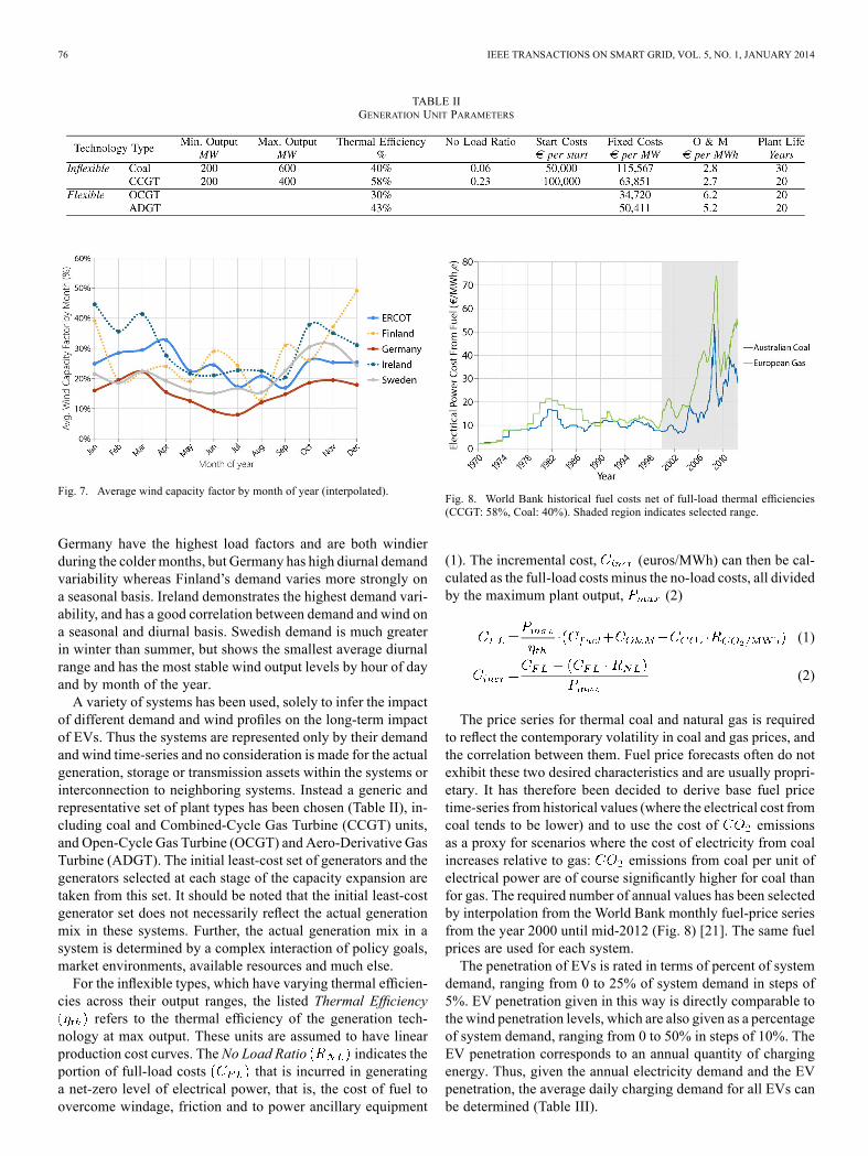
Fig. 8. World Bank historical fuel costs net of full-load thermal efficiencies(CCGT: 58%, Coal: 40%). Shaded region indicates selected range.

(1). The incremental cost, (euros/MWh) can then be cal-culated as the full-load costs minus the no-load costs, all dividedby the maximum plant output, (2)

(1)

(2)

The price series for thermal coal and natural gas is requiredto reflect the contemporary volatility in coal and gas prices, andthe correlation between them. Fuel price forecasts often do notexhibit these two desired characteristics and are usually propri-etary. It has therefore been decided to derive base fuel pricetime-series from historical values (where the electrical cost fromcoal tends to be lower) and to use the cost of emissionsas a proxy for scenarios where the cost of electricity from coalincreases relative to gas: emissions from coal per unit ofelectrical power are of course significantly higher for coal thanfor gas. The required number of annual values has been selectedby interpolation from the World Bank monthly fuel-price seriesfrom the year 2000 until mid-2012 (Fig. 8) [21]. The same fuelprices are used for each system.The penetration of EVs is rated in terms of percent of system

demand, ranging from 0 to 25% of system demand in steps of5%. EV penetration given in this way is directly comparable tothe wind penetration levels, which are also given as a percentageof system demand, ranging from 0 to 50% in steps of 10%. TheEV penetration corresponds to an annual quantity of chargingenergy. Thus, given the annual electricity demand and the EVpenetration, the average daily charging demand for all EVs canbe determined (Table III).


TABLE IIIELECTRIC VEHICLE INPUT DATA. EXAMPLE USING SCALED ERCOT DEMAND

AND TEXAS TRANSPORT DATA [24]–[26]

Fig. 9. Percentage of EVs that are connected to the power system at homecharging points each day.

For simplicity, the state-of-charge of individual batteries isnot considered. Instead it is assumed that the daily EV chargingdemand is equal to the daily average of the annual chargingdemand. Since the vehicles just replenish what they use, thestate-of-charge of the batteries will not exceed capacity. Also,assuming a vehicle is fully charged to its maximum desired levelon some date, replenishing the energy that was used will ensurethat the battery returns to this state each day.The rate of charging is constrained by a charging availability

series, i.e. the percentage of vehicles that are connected to acharging point at each hour of the day (Fig. 9). The series is de-rived from US census data [22] which gives the percentage ofrespondents leaving for work during defined time-ranges. It isthen assumed that on average, vehicles return 9 hours after theirdeparture, corresponding roughly to an 8 hour working day plustwice the average commute time. This characterization of EVavailability assumes every vehicle is a commuter vehicle andthat there are no non-commuting trips. Each grid-connected ve-hicle is assumed to be able to charge at 3.3 kW, reflecting currentlevel 2 charging capabilities [23]. It should be noted that thereis a variety of EV charging standards and capabilities. Addi-tionally, charging rates are constrained by the maximum ratingson the distribution networks to which the EVs are connected.Finally, there will be situations where the state-of-charge of abattery is too high to provide a full rate of charge for the pe-riod the vehicle is grid-connected. Thus the system chargingavailability series will be somewhat overstated. However, sincevehicles will tend to be grid-connected for long periods, andthus average charging rates will tend to be quite low, it is un-likely that charging availability will significantly constrain ve-hicle charging. Given the average annual distance traveled by

TABLE IVELECTRIC VEHICLE IMPACT QUANTIFIED OVER FOLLOWING PARAMETER SET

each vehicle (km/year), and an average vehicle efficiency (kWh/km), the number of vehicles can be determined (Table III). Incombination with the charging availability series (in %), themaximum charging power at each hour can be determined. Thecharging availability series offers the greatest charging avail-ability at hours where charging demand will tend to be at itshighest.Electricity demand tends to be highest in the evenings and is

at its lowest during the night. To reflect this, the 24-hour periodover which vehicle charging is scheduled is offset by 6 hours,such that it starts and ends at 6 pm. This tends to place the night-time demand minimum roughly in the centre of the chargingperiod whilst aligning the start of the charging period with themean home arrival time. All of the charging for a particular daymust take place within this charging window.The complete long-term impact of EVs is isolated by calcu-

lating the difference in costs, both fixed and variable, over a tenyear period, between a scenario with a particular EV penetra-tion and the same scenario with no EVs. This is presented as theaverage annual increase in system costs, per vehicle and willbe referred to herein as the Electric Vehicle Impact (EVI). Thismetric has been quantified over an extensive set of parameters(Table IV).

IV. RESULTS

A. EVI in Base Configuration

First, EVI, which is equivalent to the net-cost to the powersystem of supplying the required EV charging energy, is pre-sented for each system in its base configuration, i.e. with nowind installed, no costs and a minimal EV penetration(0.5%) (Fig. 10). The left column in each pair gives EVIunder the assumption of controlled charging, as described inSection II. The right column again presents EVI but wherecharging is uncontrolled. Here it is assumed that vehicles begincharging on home arrival (according to the commuter modeldescribed in Section III) at the maximum rate (3.3 kW) untilthe average daily vehicle energy use (11.4 kWh) has beenreplenished. This corresponds to 3.45 hours of charging foreach vehicle. It can be seen that controlled charging yieldssubstantial savings, but that the level of saving varies stronglybetween systems.Moreover, the level of EV impact can be extremely sensitive

to changes in any of the input parameters. With respect to thebase configuration, as the number of EVs is increased at a highresolution (Fig. 11), step changes in EVI can be seen, which area response to changes in the final set of generators arising fromthe capacity expansion. Thus the chosen EV penetration in thebase configuration can have a dramatic effect on the base EVI.


Fig. 10. Electric vehicle impact for controlled charging (left column in eachpair) and uncontrolled charging (right column in each pair) in the base configu-ration (0.5% EVs, 0% wind penetration, euros 0 cost).

Fig. 11. EV impact as a function of increasing EVs for all demand series (0%wind penetration, euros 0 cost, 0–5% EVs). The lighter plots represent theuncontrolled charging case. The dark plots to the front represent the controlledcharging case.

Fig. 12. Annual per-vehicle impact as a function of EV penetration for all sys-tems (0% wind penetration, euros 30 cost).

B. EVI Against EV Penetration

Next, it is shown (Fig. 12) how the impact of EVs is influ-enced by the EV penetration.Initial increments of EV demand will tend to increase the

daily net-demand floor the most owing to the triangular or“U-shaped” geometry of troughs, which increases in widthtowards the top (Fig. 13). Subsequent increments will increaseit less but will also tend to increase the production from lowermerit (higher unit cost) generation plant. As ever more incre-

Fig. 13. Additions of equal increments of EV demand to a net-demand time-series (Ireland, 2008, 46% wind penetration) leading to successively smallerincreases in minimum net-demand over the optimization horizon.

Fig. 14. Annual per-vehicle impact as a function of wind penetration for allsystems (5% EV penetration, euros 0 cost).

ments are added, extra EV demand may even exacerbate peaks,forcing unit starts or even necessitating extra capacity wherecharging occurs at the annual peak. All of these effects meanthat as EV demand increases on a system, the cost of meetingthe extra demand will tend to increase also.This is reflected in Fig. 12 where the impact of EVs increases

for all systems as EV penetration increases. This relationshipis generally replicated across the input set. The only exceptionsare where an incremental increase in EV load leads to a largestep-change in the optimal set of generation plant.

C. EVI Against Wind Penetration

The addition of wind plant can lead to more erratic changes inElectric Vehicle Impact (Fig. 14). At higher wind penetrationsthere is increased net-demand variability. Since EVs can reducethis variability, with an accompanying reduction in costs, EVIshould be higher as wind levels increase. However, increases invariable generation also reduce the utilization of conventionalgenerating units. The viability of high fixed cost generation re-lies on high capacity factors, however the most suitable planttypes to take the place of high fixed cost units is not obvious.As an example (Fig. 15), when the capacity of coal falls in thefinal optimal plant mix, there is an increase in CCGT generationwhile there are oscillations in ADGT and CCGT capacity.At higher cost levels, a more stable dynamic is seen

(Fig. 16). Higher costs relatively affect coal investmentto the greatest extent and in this case there are no coal units


Fig. 15. Final levels of installed plant for increasing levels of installed wind(Sweden, 5% EV penetration, euros 0 cost).

Fig. 16. Annual per-vehicle impact as a function of wind penetration for allsystems (5% EV penetration, euros 30 cost).

Fig. 17. Final levels of installed plant for increasing levels of installed wind(Sweden, 5% EV penetration, euros 30 cost).

in the final plant mix. Since the installed capacity of only oneinflexible generation type (i.e. CCGT) increases, changes inEV impact are more consistent and accord to expectations. Thechanges in the optimal set of generators (Fig. 17), whilst large,are stable across the range of wind penetrations.

D. EVI Against Cost

The greatest level of volatility in Electric Vehicle Impact oc-curs where the relative price of coal and gas is such that changesin either price will lead to large changes in the optimal capacityof generation from the fuels. Changes in the relative price ofthe fuels can be represented by varying the cost of per-mits, since the cost of relatively affects the price of coal

Fig. 18. Annual per-vehicle impact as a function of cost for all EV pen-etrations (Ireland, 10% wind penetration).

Fig. 19. Hourly costs (sum of no-load and incremental costs) as a function ofgenerator electrical output for each generation type .

Fig. 20. Final installed capacities for selected cost levels and electricvehicle penetrations (Ireland, 10% wind).

more than the price of gas (coal releases more per unit ofenergy than natural gas).Fig. 18 presents EVI as a function of cost. A large spike

in vehicle impact occurs in the region of 20–30 euros/t, .At 20 euros/t, , CCGT generation begins to offer lowercost power than coal at high output levels (Fig. 19). Neverthe-less, the coal units have lower start costs (Table II) and sincethey are competitive at low output levels, they still appear inthe least-cost set of generators (Fig. 20). However, at 30 euros/t,

, coal generation is much more costly than production from


Fig. 21. Electric vehicle impact for optimal and uncontrolled charging cases.

CCGT units and thus no longer appears at all in the final gener-ation mix (Fig. 20).The step-changes in EVI between 20 and 30 euros/t,

occur because much of the EV demand will be met by gener-ation that would have been online in the absence of any EVs.Incremental costs are a much smaller fraction of full-load costsfor CCGT plants than for coal plants, thus EVI is often lower inhigh net-demand variability cases where CCGT is the dominantbaseload technology.The final result returns to the comparison made at the start of

the section between controlled and uncontrolled charging. Sincefull user participation in direct or indirect charging control maynot be feasible, this provides a worst-case scenario in that re-spect. The average EVI (presented here in units of euros/MWh)for the controlled charging case is 51.5 euros/MWh (rangingfrom 20.8 to 77.5 euros/MWh). For the uncontrolled case, theaverage is far higher, averaging 94.1 euros/MWh and rangingfrom 45.7 to 120.4 euros/MWh). This indicates that there maybe a sufficient incentive for system operators to establish somelevel of direct or indirect control over EV charging.

V. CONCLUSIONS

This paper has sought to determine the cost of electric ve-hicle charging, once the potential mutual benefits between thevehicles and the power generation fleet have been taken into ac-count. When charged in a manner that is optimal to the powersystem, EVs can increase generator capacity factors and reducecostly baseload starts and part-loading. In the long-term, this

will encourage increased investment in higher efficiency plants,which may be more costly to cycle and require higher levels ofutilization to justify their installed cost.The net-cost of EV charging, termed the Electric Vehicle Im-

pact, is found to vary significantly across a number of param-eters. First, the particular characteristics of demand variabilityare important: greater seasonality leads to increased chargingby peaking generation, reducing EV benefit, whilst increaseddiurnality increases baseload cycling, which provides the op-portunity for EVs to reduce costs. Second, Greater numbers ofEVs will tend to lead to diminishing returns from EVs, owingpartly to the inherent geometry of demand troughs but also sinceadditional increments of charging use successively lower-meritgeneration. Third, increased wind penetration will tend to in-crease EV benefit, but can also incentivize the provision of moreflexible generation, which has less to gain from EVs and tendsto cost the system more. Finally, the relative level of fuel costs,which is affected by the cost of emissions, can dictate verylarge changes in the installed set of generators over time, whichwill favor EVs where the changes would lead to increases in cy-cling costs.The need for unit-commitment and the breadth of scenarios

studied meant that a conventional methodology would be com-putationally impractical. A new unit-commitment algorithm hastherefore been developed for this purpose. A methodology suchas this could be used to inform the design of tariffs for electricvehicle charging, returning some of the potential benefits of op-timized charging to the vehicle user.


VI. FUTURE WORK

Specific systems present specific challenges and allow for theopportunity to consider an expanded range of generation andancillary technologies. For example, solar power presents verydifferent statistical properties to wind. This may require dataat higher resolutions and different modeling approaches. Eachsystem presents unique constraints and topologies at the trans-mission and distribution levels. Thus, the charging regimes herecan be contrasted to charging strategies that are optimal with re-spect to particular network configurations.EVs are one of many sources of power system flexibility. Ide-

ally these should all be considered together, in particular whereflexibility may be the primary purpose of a particular invest-ment, e.g. pumped storage or HVDC lines.An attractive feature of EVs is the elimination of point-of-use

emissions. Additional system demand will lead to an increasein emissions of and changes in levels of other pollutants,and so the net-emissions in each emissions category should becalculated. This could build upon the work of [16].There are certain assumptions that have been made in this

analysis which could be investigated in more depth. For ex-ample, using higher resolution wind and demand time-seriesmay lead to increased cycling costs, reducing EV impact further.Finally, least-cost investment has been assumed here, but

there are many reasons why actual investment will differ.Thus the impact of EVs under different market and regulatoryarrangements would be worth pursuing.

APPENDIX APERFORMANCE OF FAST ALGORITHM

The FAST algorithm can be compared to its equivalent MIPformulation in terms of the optimality of the schedules (the de-gree to which cost are minimized), the similarity of the sched-ules and finally, the computation time. First, the formulation ofthe equivalent is given.

A. Equivalent MIP Formulation

The objective function (3) is the sum of hourly productioncosts for the whole year.

(3)

The hourly costs (4) equal the costs from the inflexible types(start, no-load and incremental costs) added to the costs for theflexible types (average costs).

(4)

The sum of production from inflexible, flexible and wind gen-eration (less curtailment) must equal the electricity demand foreach hour (5).

(5)

Wind curtailment (6) must be less than or equal to wind pro-duction in each hour.

(6)

The sum of online inflexible capacity less the sum of inflex-ible production (i.e. the quantity of spinning reserve) must ex-ceed a pre-defined target (7). For simplicity, here this target isset to the size of the largest installed unit, where at least onesuch unit exists.

(7)Production from any type cannot exceed the quantity in-

stalled. Similarly, the number of online inflexible units cannotexceed the number installed (8).

(8)

(9)

Production from any inflexible type is bounded by minimum(10) and maximum (11) output levels and the number of onlineunits of that type.

(10)

(11)

Finally, the number of starts for an inflexible type isset to the increase in the number of online units forthat type (12).

(12)

B. Performance Comparison

The FAST algorithm and its equivalent MIP is comparedacross a broad range of input parameters. For 3 plant types(coal, CCGT, OCGT), all combinations of plant equalling11.8 GW installed capacity (271) are considered on the 5systems-ERCOT, Finland, Germany, Ireland, Sweden—whereeach demand-series is scaled to 10 GW peak. 6 levels of in-stalled wind (0 GW to 10 GW in steps of 2 GW) and a cost-setreflecting recent European fuel spot prices is used [27].1) Optimality: A MIP is usually not solved to optimality.

Instead, once a set of decision variable values is found such thatthe objective function value of the MIP is within some toleranceof the objective function value of the the solution of the relaxedform of theMIP, the solution is accepted as integer optimal. Thistolerance is called the optimality gap. An equivalent optimalitygap can be calculated for schedules from the FAST algorithm tocompare the optimality of the methods. In order to focus on theimportant plant combinations, for each system and wind level,the optimality gap for both methods is given for the ten lowesttotal costs plant combinations (Fig. 22).2) Similarity: To compare the similarity of the unit-commit-

ments from the two methods, the total online inflexible capacityfor the ten lowest total cost plant combinations is presented inFig. 23 for each system and wind combination.


Fig. 22. Optimality gap for FAST and equivalent MIP, averaged over the tengeneration plant combinations with lowest total costs.

Fig. 23. Mean combined CCGT and coal online capacity for FAST and equiv-alent MIP, averaged over the ten plant combinations with lowest total costs.

TABLE VCOMPUTATION TIME STATISTICS FOR THE MIP AND THE FAST ALGORITHM

3) Computation Time: Finally, the computation time is com-pared for all of the plant combinations considered (Table V). Itis seen that the computation time for the equivalent MIP is overa thousand times longer than for the FAST algorithm.The much reduced computation time for the algorithm

is achieved by utilizing a logical structure that requires theconsideration of only a relatively small number of potentialcommitments, i.e. those that could potentially reduce costs. Anexample of this is the use of the relative magnitude of net-ca-pacity demand and online inflexible capacity as a criterion forconsidering changes in the commitment (Fig. 2).

APPENDIX BPORTFOLIO TRAJECTORY EXAMPLE

Given the number of cases considered, it is not possible topresent the generation portfolio trajectory for each case. Never-theless, an example of how the portfolio adapts to the additionof EVs is given to provide insight into this process. The chosencase, which appears in the text of Section IV-D and to varyingdegrees in Figs. 18–20, represents the Ireland, 10% wind pene-tration, 25% EV penetration and 20 euros/t tax case.It is seen (Fig. 24) that the large-scale introduction of EVs re-

duces the need for coal’s part-loading performance and enablesthe introduction of CCGT generation, which for this costlevel offers the lowest production costs at higher loading levels(see Fig. 19).

Fig. 24. Installed capacity of each generation type for each year of the studyperiod (Ireland, 10% wind, 25% EVs, ).

TABLE VIYEAR OF RETIREMENT FOR EACH INFLEXIBLE UNIT. A RETIREMENT YEAR ISPROVIDED FOR EACH UNIT UP TO A MAXIMUM OF 16 INSTALLED UNITS OF

EITHER TYPE

TABLE VIIYEARS AT WHICH BLOCKS OF CAPACITY OF EACH TYPE ARE RETIRED

APPENDIX CRETIREMENT SCHEDULES

Generation capacity is retired according to pre-defined retire-ment schedules. This is done so that capacity retirements do notvary across the studied cases. It is assumed that the capacity ex-pansionduration (10years)dividedby the lifeof theplant inques-tion (30years for coal, 20years for theCCGT,ADGTandOCGT)gives the fraction of capacity of that type that will be retired overthe period. Thus, 1/2 of the initial CCGT, OCGT and ADGT ca-pacitywill retire and1/3of the coal capacitywill retireover the10year capacity expansion period. When an expansion in capacityis required, the candidate optionswill be considered for the life ofthe longest plant under consideration, which is usually 30 years.Retirements that would occur over that period are not consideredat that point though, since that would require expansions withinexpansions. Since the initial capacity of each plant type variesbased on the demand andwind series used, each unit is numberedand has a year that it will retire in, if it is installed (see Table VI).For example, if there are6 coalplants in the initial portfolio, 2willretire. The first will retire in year zero and the second in year 5.The flexible types are retired in two blocks (Table VII). The

purpose of doing this is to have certain years where larger


amounts of capacity retires, which reduces the impact of theintegral nature of unit expansions. For example, where there is a400 MW deficit, a 400 MW CCGT plant will have a significantadvantage over a 600 MW coal unit.

REFERENCES[1] “Environmental Assessment of Plug-In Hybrid Electric Vehicles,”

Electric Power Research Institute, Tech. Rep., Palo Alto, CA, USA,2007.

[2] U. Bossel, “The hydrogen illusion: Why electrons are a better energycarrier,” Cogeneration and On-Site Power Production, pp. 55–59,2004.

[3] K. Parks, P. Denholm, and A. J. Markel, “Costs and Emissions As-sociated With Plug-In Hybrid Electric Vehicle Charging in the XcelEnergy Colorado Service Territory,: National Renewable Energy Lab-oratory (NREL), Tech. Rep., 2007.

[4] P. Denholm and W. Short, “Evaluation of Utility System Impacts andBenefits of Optimally Dispatched Plug-In Hybrid Electric Vehicles(Revised),” National Renewable Energy Laboratory (NREL), Tech.Rep., 2006.

[5] J. P. Lopes, F. J. Soares, and P. R. Almeida, “Integration of electricvehicles in the electric power system,” Proc. IEEE, vol. 99, no. 1, pp.168–183, 2011.

[6] “Damage to Power Plants Due to Cycling,” Electric Power ResearchInstitute, Tech. Rep., Palo Alto, CA, USA, 2001.

[7] “Correlating Cycle Duty With Cost at Fossil Fuel Power Plants,” Elec-tric Power Research Institute, Tech. Rep., Palo Alto, CA, USA, 2001,Tech. Rep..

[8] N. Troy, E. Denny, and M. O’Malley, “Base-load cycling on a systemwith significant wind penetration,” IEEE Trans. Power Syst., vol. 25,no. 2, pp. 1088–1097, 2010.

[9] Commercial Offer Data—Standard Generator Single ElectricityMarket Operator, Ireland, Last accessed November 2012 [Online].Available: http://www.sem-o.com/marketdata/Pages/PricingAnd-Scheduling.aspx

[10] A. Shortt and M. O’Malley, “Impact of optimal charging of electricvehicles on future generation portfolios,” in Proc. Conf. SustainableAlternative Energy (SAE), 2009 IEEE PES/IAS, Sep. 2009, pp. 1–6.

[11] W. Short and P. Denholm, “Preliminary Assessment of Plug-In HybridElectric Vehicles on Wind Energy Markets,” National Renewable En-ergy Laboratory (NREL), Tech. Rep., Golden, CO, USA, 2006.

[12] P. Denholm and W. Short, “Evaluation of Utility System Impacts andBenefits of Optimally Dispatched Plug-In Hybrid Electric Vehicles(Revised),” National Renewable Energy Laboratory (NREL), Tech.Rep., Golden, CO, USA, 2006.

[13] J. Kiviluoma and P. Meibom, “Influence of wind power, plug-in elec-tric vehicles, and heat storages on power system investments,” Energy,vol. 35, no. 3, pp. 1244–1255, 2010.

[14] A. Shortt, J. Kiviluoma, and M. O’Malley, “Accommodating vari-ability in generation planning,” IEEE Trans. Power Syst., vol. 28, no.1, pp. 158–169, Feb. 2013.

[15] CPLEX 12, Section: Mixed-Integer Programming IBM ILOG [On-line]. Available: http://www.gams.com/dd/docs/solvers/cplex.pdf

[16] R. Sioshansi and P. Denholm, “Emissions impacts and benefits ofplug-in hybrid electric vehicles and vehicle-to-grid services,” Environ.Sci. Technol. vol. 43, no. 4, pp. 1199–1204, 2009 [Online]. Available:http://pubs.acs.org/doi/abs/10.1021/es802324j

[17] C.Gellings, “The concept of demand-sidemanagement for electric util-ities,” Proc. IEEE, vol. 73, no. 10, pp. 1468–1470, 1985.

[18] “Cost and Performance for Power Generation Technologies,” Pre-pared for the National Renewable Energy Laboratory by Black& Veatch, (Feb. 2013) [Online]. Available: http://bv.com/docs/re-ports-studies/nrel-cost-report.pdf

[19] Generator Data Parameters “All Island Project,”, (Nov.2012) [Online]. Available: http://www.allislandpro-ject.org/zip/Datasheets%20Public.zip

[20] W.Katzenstein, E. Fertig, and J. Apt, “The variability of interconnectedwind plants,” Energy Policy, vol. 38, no. 8, pp. 4400–4410, 2010.

[21] Monthly World Prices of Commodities and Indices World Bank, (Aug.2012) [Online]. Available: http://siteresources.worldbank.org/INT-PROSPECTS/Resources/334934-1304428586133/PINK_DATA.xlsx

[22] Journey to Work: (Census 2000 Brief) United States Census Bureau,USA, (Jul. 2011) [Online]. Available: http://www.census.gov/prod/2004pubs/c2kbr-33.pdf

[23] M. Yilmaz and P. Krein, “Review of battery charger topologies,charging power levels, and infrastructure for plug-in electric andhybrid vehicles,” IEEE Trans. Power Electron., vol. 28, no. 5, pp.2151–2169, May 2013.

[24] Office of Highway Policy Information-Highway Statistics Series Fed-eral Highway Administration, USA, (Aug. 2012) [Online]. Available:http://www.fhwa.dot.gov/policyinformation/statistics/abstracts/tx.cfm

[25] Nissan Leaf Specifications Nissan, (Aug. 2012) [Online]. Available:http://www.nissan.ie/vehicles/leaf/

[26] Mitsubishi i-MiEV Specifications Mitsubishi Motors, (Aug. 2012)[Online]. Available: http://i.mitsubishicars.com/miev/features/com-pare/

[27] Natural Gas Spot & Coal Futures Prices European Energy Exchange,(Dec. 2010) [Online]. Available: http://www.eex.com/

Aonghus Shortt (S’09) received the B.E. degree from University CollegeDublin, Dublin, Ireland, in 2008, where he is currently pursuing the Ph.D.degree with research interests in electric vehicles, wind power generation andpower system planning and investment.

Mark O’Malley (F’07) received the B.E. and Ph.D. degrees from UniversityCollege Dublin, Dublin, Ireland, in 1983 and 1987, respectively.He is currently Professor of Electrical Engineering at University College

Dublin and director of the Electricity Research Centre with research interest inpower systems, control theory, and biomedical engineering.

Documents

Quantifying the Long-Term Impact of Electric Vehicles on the Generation Portfolio