QUANTIFYING THE ECONOMIC VALUE OF WEATHER FORECASTS: REVIEW OF METHODS AND RESULTS

Rick Katz

Institute for Study of Society and Environment National Center for Atmospheric Research

Boulder, CO USA

Email: rwk@ucar.edu Web site: www.isse.ucar.edu/HP_rick.html Lecture: www.isse.ucar.edu/HP_rick/pdf/ukkatz.pdf

Quote

“You don’t get points for predicting rain. You get points for building

arks.”

Lou Gerstner (Former IBM CEO)

Outline

(1) Motivation (2) Prescriptive Decision-Making Framework (3) Economic Value of Forecasts (4) Protypical Decision-Making Models (5) Quality-Value Relationships (6) Valuation Puzzles (7) Review of Case Studies (8) Discussion

(1) Motivation

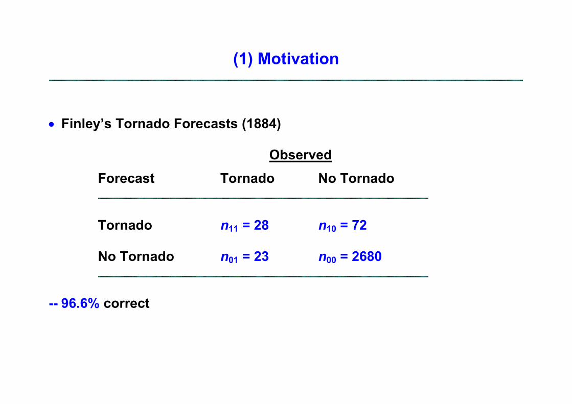
• Finley’s Tornado Forecasts (1884)

Observed Forecast Tornado No Tornado

Tornado n11 = 28 n10 = 72

No Tornado n01 = 23 n00 = 2680

-- 96.6% correct

(1) Motivation

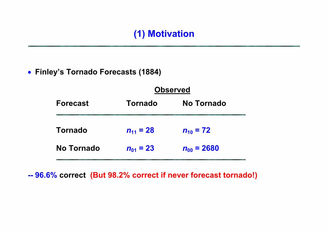
• Finley’s Tornado Forecasts (1884)

Observed

Forecast Tornado No Tornado

Tornado n11 = 28 n10 = 72

No Tornado n01 = 23 n00 = 2680

-- 96.6% correct (But 98.2% correct if never forecast tornado!)

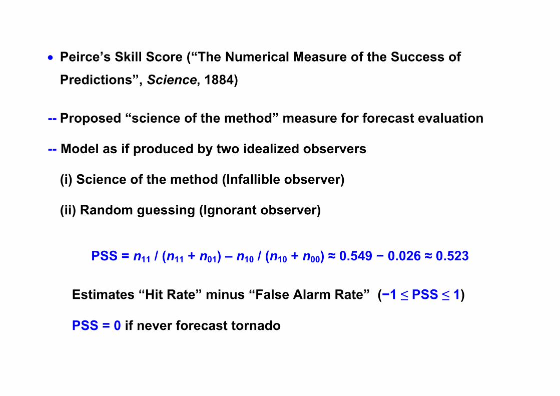
• Peirce’s Skill Score (“The Numerical Measure of the Success of Predictions”, Science, 1884)

-- Proposed “science of the method” measure for forecast evaluation

-- Model as if produced by two idealized observers (i) Science of the method (Infallible observer) (ii) Random guessing (Ignorant observer)

PSS = n11 / (n11 + n01) – n10 / (n10 + n00) ≈ 0.549 − 0.026 ≈ 0.523

Estimates “Hit Rate” minus “False Alarm Rate” (−1 ≤ PSS ≤ 1)

PSS = 0 if never forecast tornado

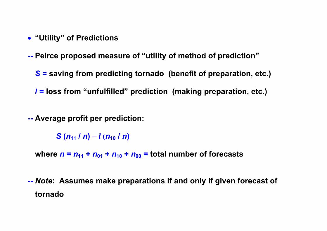
• “Utility” of Predictions

-- Peirce proposed measure of “utility of method of prediction” S = saving from predicting tornado (benefit of preparation, etc.) l = loss from “unfulfilled” prediction (making preparation, etc.) -- Average profit per prediction: S (n11 / n) − l (n10 / n) where n = n11 + n01 + n10 + n00 = total number of forecasts -- Note: Assumes make preparations if and only if given forecast of

tornado

(2) Prescriptive Decision-Making Framework

• Elements of Decision Making -- Events (Θ = θ)

Adverse weather event (such as “Rain”)

-- Actions (a) Protection (to prevent or reduce impact of event)

-- Consequences [w(a, θ)] Action-Event pair

• Forecast Information System

-- Forecast Weather (Z = z)

Conditional probability distribution for event Z = z indicates forecast for particular occasion Specifies conditional distribution of weather (Θ │Z = z) Systems viewpoint: Also need unconditional distribution of Z

-- Climatological Information (“Climatology”)

Unconditional probability distribution of Θ

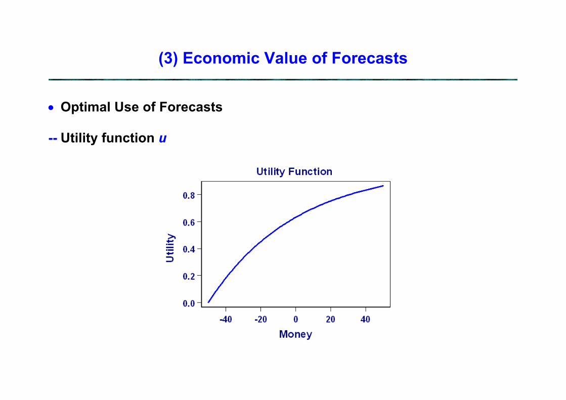
(3) Economic Value of Forecasts

• Optimal Use of Forecasts

-- Utility function u

-- Risk neutral

u linear function (suffices to work in monetary terms)

-- Risk aversion u concave function (figure above)

-- Risk taking

u convex function

-- Payoff (utility function evaluated at consequence) u[w(a, θ)]

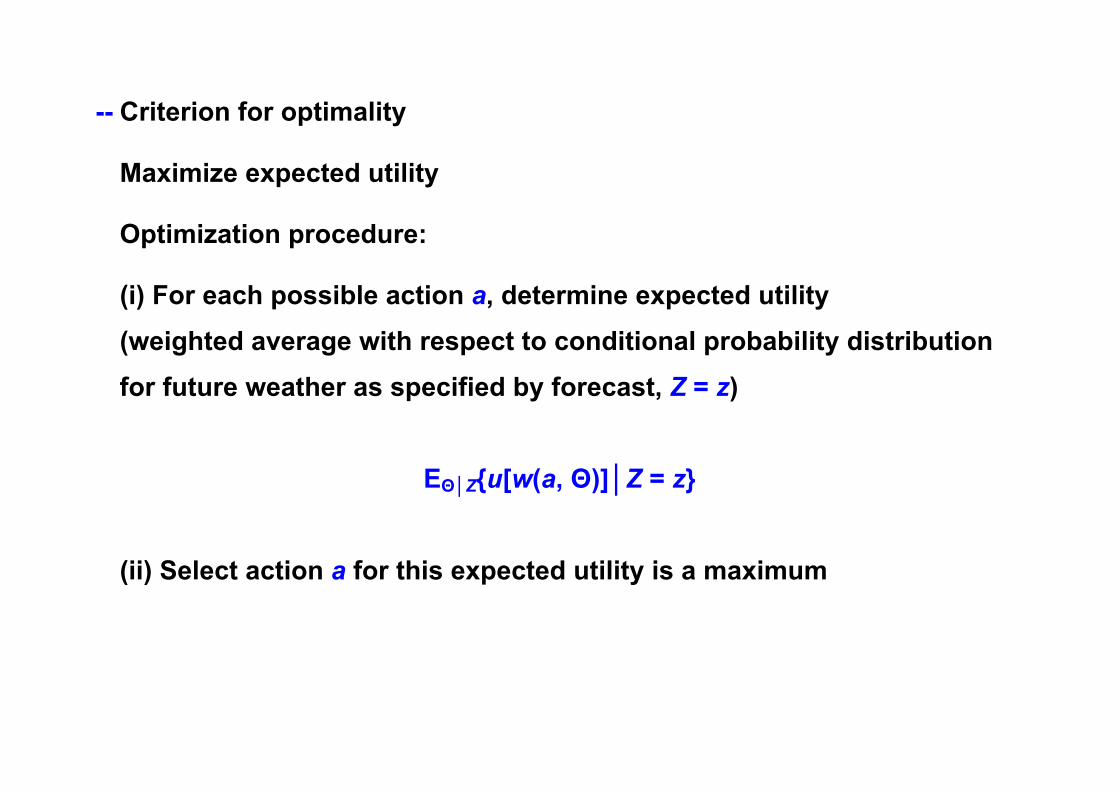
-- Criterion for optimality

Maximize expected utility

Optimization procedure: (i) For each possible action a, determine expected utility (weighted average with respect to conditional probability distribution for future weather as specified by forecast, Z = z)

EΘ│Z{u[w(a, Θ)]│Z = z}

(ii) Select action a for this expected utility is a maximum

• Economic Value of Forecasts -- Standard of Comparison

e. g., climatological information

Other examples (“persistence”, alternative forecasting system)

-- Concept of Value of Imperfect Information (VOI)

Measure of how much better off decision maker is

(with vs. without forecasting system)

e. g., increase in expected return (or reduction in expected expense) for forecasting system as compared to climatology

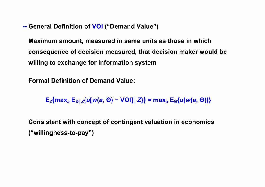
-- General Definition of VOI (“Demand Value”)

Maximum amount, measured in same units as those in which consequence of decision measured, that decision maker would be willing to exchange for information system

Formal Definition of Demand Value:

EZ(maxa EΘ│Z{u[w(a, Θ) − VOI]│Z}) = maxa EΘ{u[w(a, Θ)]}

Consistent with concept of contingent valuation in economics (“willingness-to-pay”)

(4) Prototypical Decision-Making Models

• Background -- Long tradition of use in valuing weather forecasts -- Still quite popular in valuing ensemble prediction systems -- Limited, if any, descriptive content • Cost-Loss Decision-Making Model -- Static decision-making structure -- Only two possible actions -- Only two possible states of weather -- Assumes linear utility function

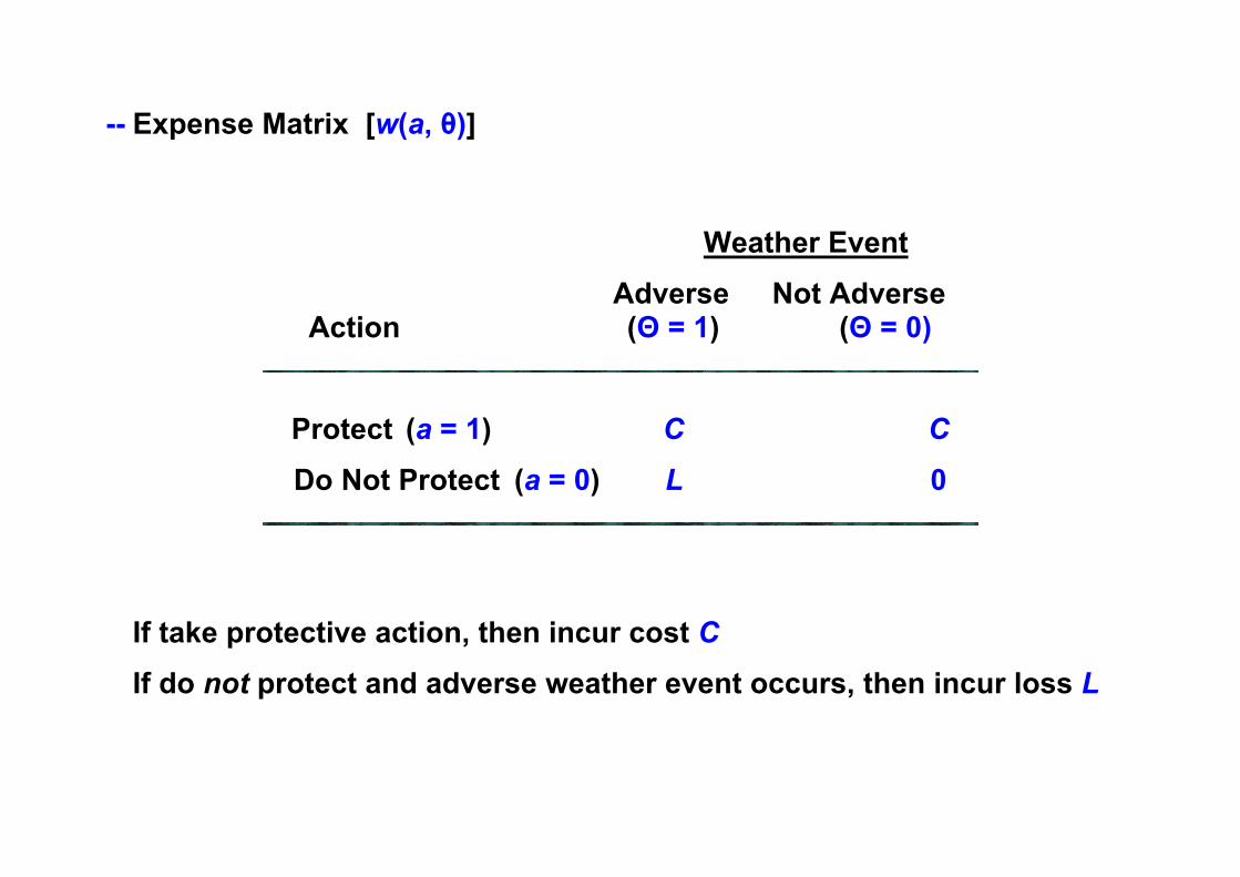
-- Expense Matrix [w(a, θ)]

Weather Event Adverse Not Adverse Action (Θ = 1) (Θ = 0)

Protect (a = 1) C C Do Not Protect (a = 0) L 0

If take protective action, then incur cost C If do not protect and adverse weather event occurs, then incur loss L

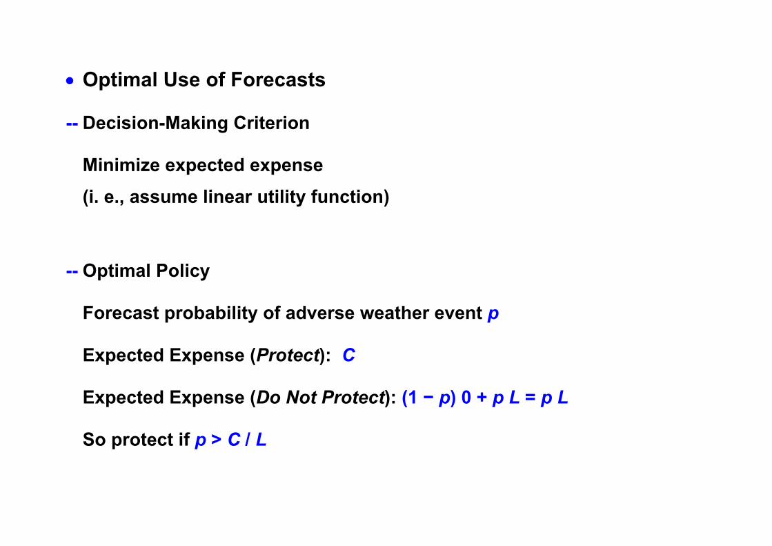
• Optimal Use of Forecasts -- Decision-Making Criterion Minimize expected expense (i. e., assume linear utility function)

-- Optimal Policy Forecast probability of adverse weather event p Expected Expense (Protect): C Expected Expense (Do Not Protect): (1 − p) 0 + p L = p L So protect if p > C / L

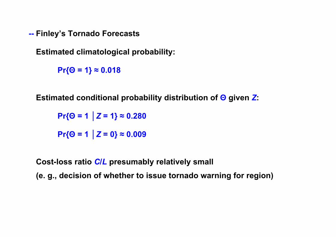
-- Finley’s Tornado Forecasts Estimated climatological probability: Pr{Θ = 1} ≈ 0.018

Estimated conditional probability distribution of Θ given Z: Pr{Θ = 1 │Z = 1} ≈ 0.280

Pr{Θ = 1 │Z = 0} ≈ 0.009

Cost-loss ratio C/L presumably relatively small (e. g., decision of whether to issue tornado warning for region)

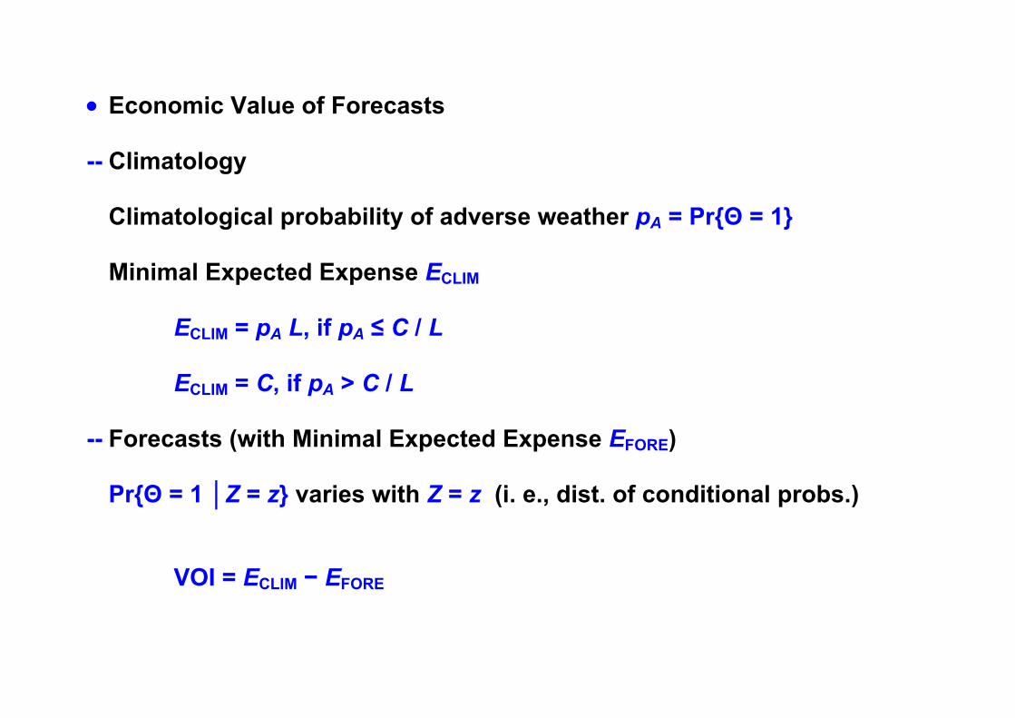
• Economic Value of Forecasts -- Climatology

Climatological probability of adverse weather pA = Pr{Θ = 1} Minimal Expected Expense ECLIM

ECLIM = pA L, if pA ≤ C / L

ECLIM = C, if pA > C / L

-- Forecasts (with Minimal Expected Expense EFORE)

Pr{Θ = 1 │Z = z} varies with Z = z (i. e., dist. of conditional probs.)

VOI = ECLIM − EFORE

• Other Prototypical Decision-Making Models -- Dynamic (instead of static) e. g., assume loss L can be incurred at most once Criterion of minimizing total expected expense over some time horizon

(perhaps discounted) Optimal policy no longer protect if p > C / L (change in threshold) Consequent effect on forecast value as well

(5) Quality-Value Relationships

• Statistical Model for Generating Probability Forecasts (e. g., from perfect numerical weather prediction system) -- Beta Distribution (for probability forecast p)

Natural distribution for probabilities, 0 < p < 1 Parameters r, s (0 < r < ∞, 0 < s < ∞)

Mean: r / (r + s)

Assume perfectly reliable probability forecasts In particular, pA = r / (r + s)

-- Climatology (i. e., no skill) r → ∞, s → ∞ (holding pA constant) -- Perfect information r → 0, s → 0 (holding pA constant) -- Brier score (BS) BS = E[(Θ − p)2]

-- Brier skill score (BSS) BSS = 1 − [BS / Var(Θ)], 0 ≤ BSS ≤ 1

Climatology: BSS = 0 Perfect information: BSS = 1 Model based on beta distribution: BSS = 1 / (r + s + 1)

0.0 0.2 0.4 0.6 0.8 1.0

Probability Forecast

0

1

2

3

4

5

Bet

a D

istr

ibu

tio

n

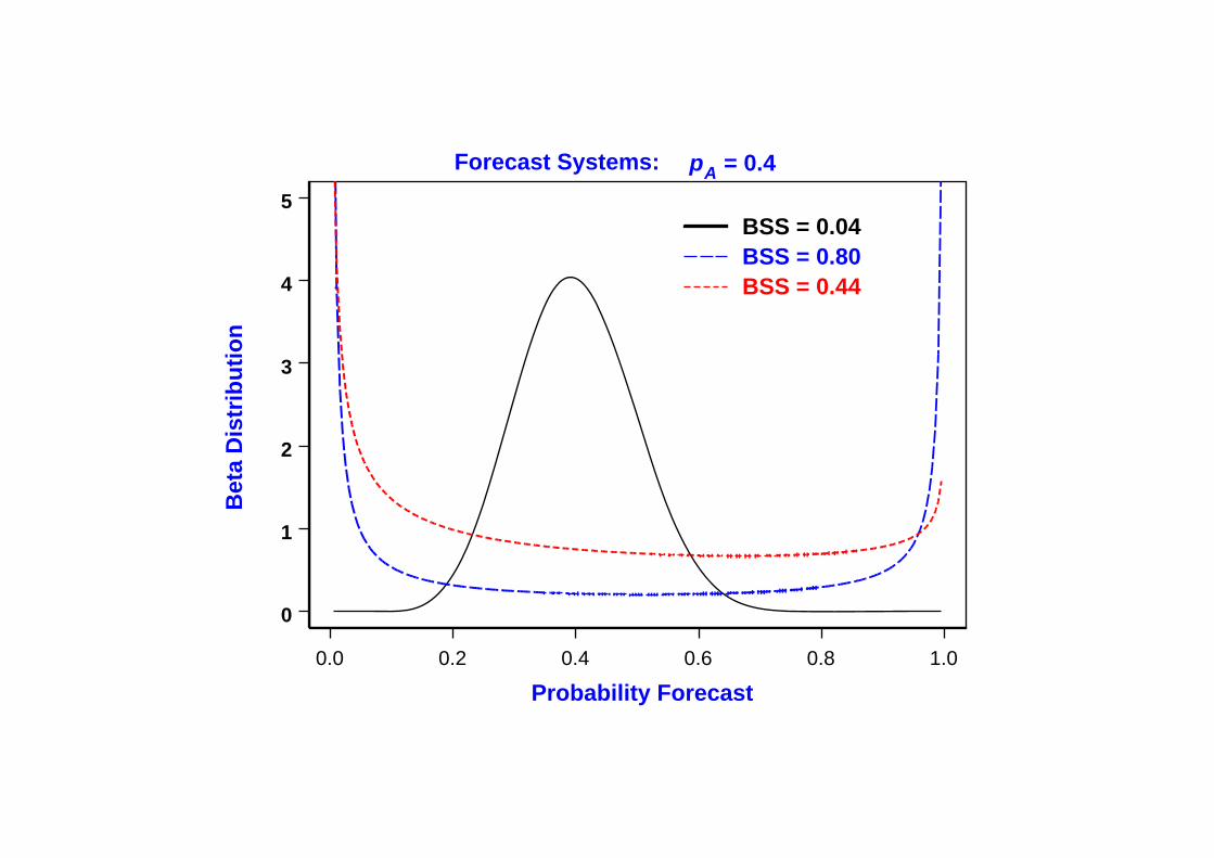
Forecast Systems:

BSS = 0.04BSS = 0.80BSS = 0.44

pA = 0.4

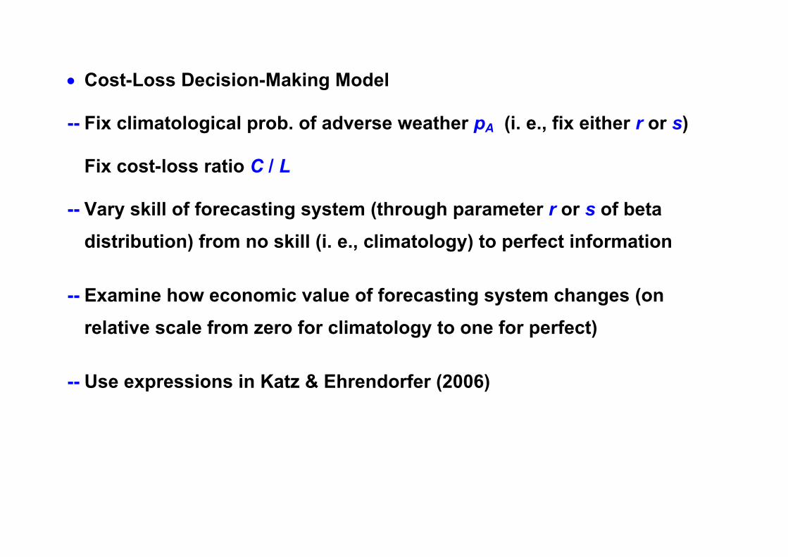
• Cost-Loss Decision-Making Model -- Fix climatological prob. of adverse weather pA (i. e., fix either r or s)

Fix cost-loss ratio C / L -- Vary skill of forecasting system (through parameter r or s of beta

distribution) from no skill (i. e., climatology) to perfect information -- Examine how economic value of forecasting system changes (on

relative scale from zero for climatology to one for perfect)

-- Use expressions in Katz & Ehrendorfer (2006)

0.0 0.2 0.4 0.6 0.8 1.0

Brier Skill Score

0.0

0.2

0.4

0.6

0.8

1.0

Rel

ativ

e E

con

om

ic V

alu

e

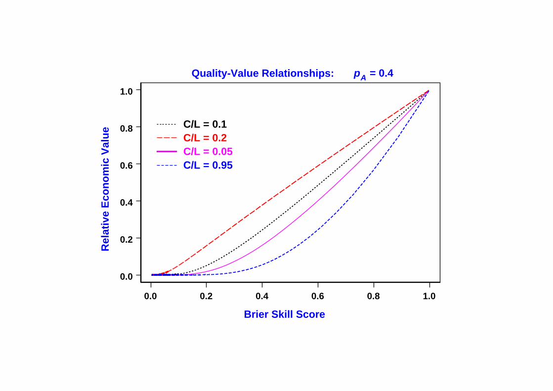
Quality-Value Relationships:

C/L = 0.1C/L = 0.2C/L = 0.05C/L = 0.95

pA = 0.4

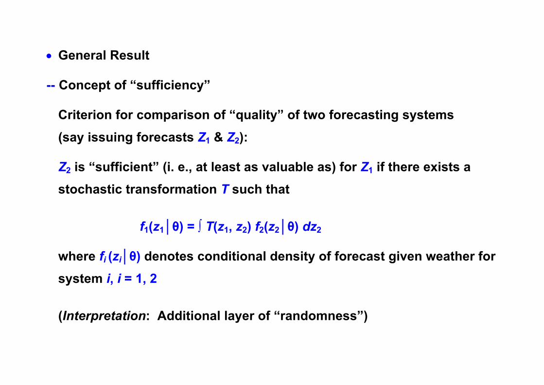
• General Result -- Concept of “sufficiency”

Criterion for comparison of “quality” of two forecasting systems (say issuing forecasts Z1 & Z2):

Z2 is “sufficient” (i. e., at least as valuable as) for Z1 if there exists a

stochastic transformation T such that f1(z1│θ) = ∫ T(z1, z2) f2(z2│θ) dz2

where fi (zi│θ) denotes conditional density of forecast given weather for system i, i = 1, 2

(Interpretation: Additional layer of “randomness”)

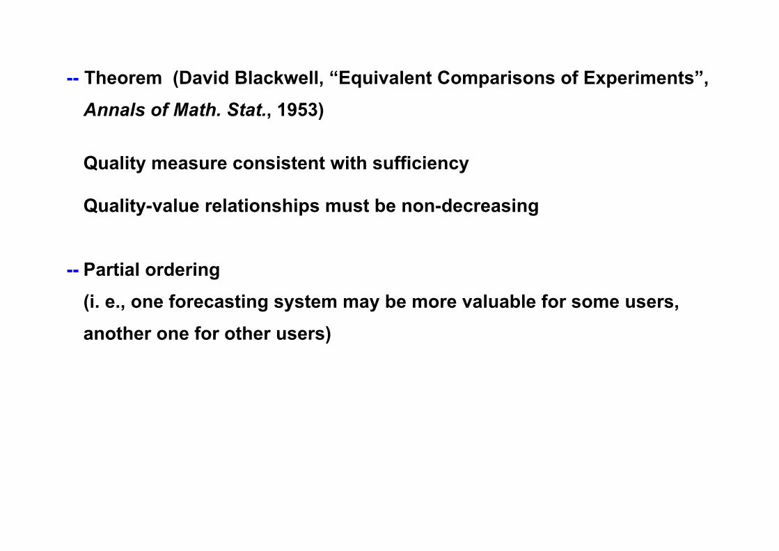
-- Theorem (David Blackwell, “Equivalent Comparisons of Experiments”, Annals of Math. Stat., 1953)

Quality measure consistent with sufficiency

Quality-value relationships must be non-decreasing

-- Partial ordering (i. e., one forecasting system may be more valuable for some users, another one for other users)

(6) Valuation Puzzles

• Quality-Value Reversals -- Ensemble prediction system Assume perfect numerical model

(apply statistical model for probability forecasts based on beta distribution)

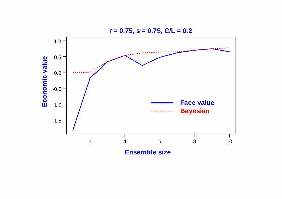
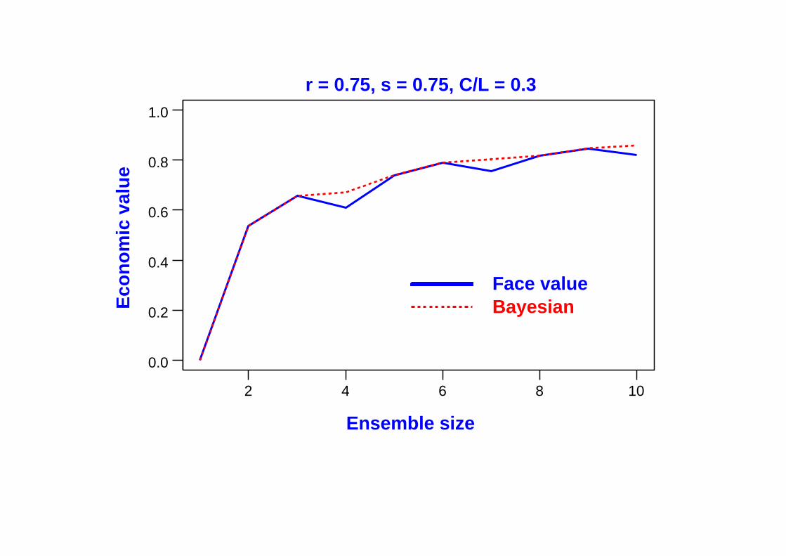
-- But now only finite number m of ensembles available

Generate these ensembles using underlying forecast probability p from beta distribution

Usual approach:

Take ensembles at “face value” Suppose event occurs for k out m ensembles Estimate forecast probability as p̂ = k/m

Alternative approach: Bayesian (in which uncertainty in estimating p also taken in account)

-- Cost-Loss Decision-Making Model Usual prototypical model for valuing ensemble forecasts

2 4 6 8 10

Ensemble size

-1.5

-1.0

-0.5

0.0

0.5

1.0E

con

om

ic v

alu

e

Face valueBayesian

r = 0.75, s = 0.75, C/L = 0.2

2 4 6 8 10

Ensemble size

0.0

0.2

0.4

0.6

0.8

1.0E

con

om

ic v

alu

e

Face valueBayesian

r = 0.75, s = 0.75, C/L = 0.3

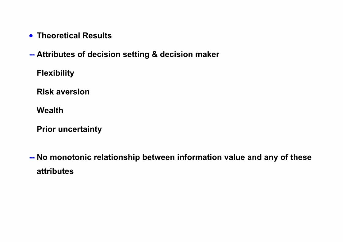
• Theoretical Results -- Attributes of decision setting & decision maker Flexibility Risk aversion

Wealth

Prior uncertainty

-- No monotonic relationship between information value and any of these attributes

(7) Review of Case Studies

• Recent Case Studies of Economic Value

-- www.isse.ucar.edu/HP_rick/esig.html Any published prescriptive study in which economic value of weather or climate forecasts quantified Earlier studies reviewed in chapter by Dan Wilks (Economic Value of Weather and Climate Forecasts, edited by Katz & Murphy, Cambridge Univ. Press)

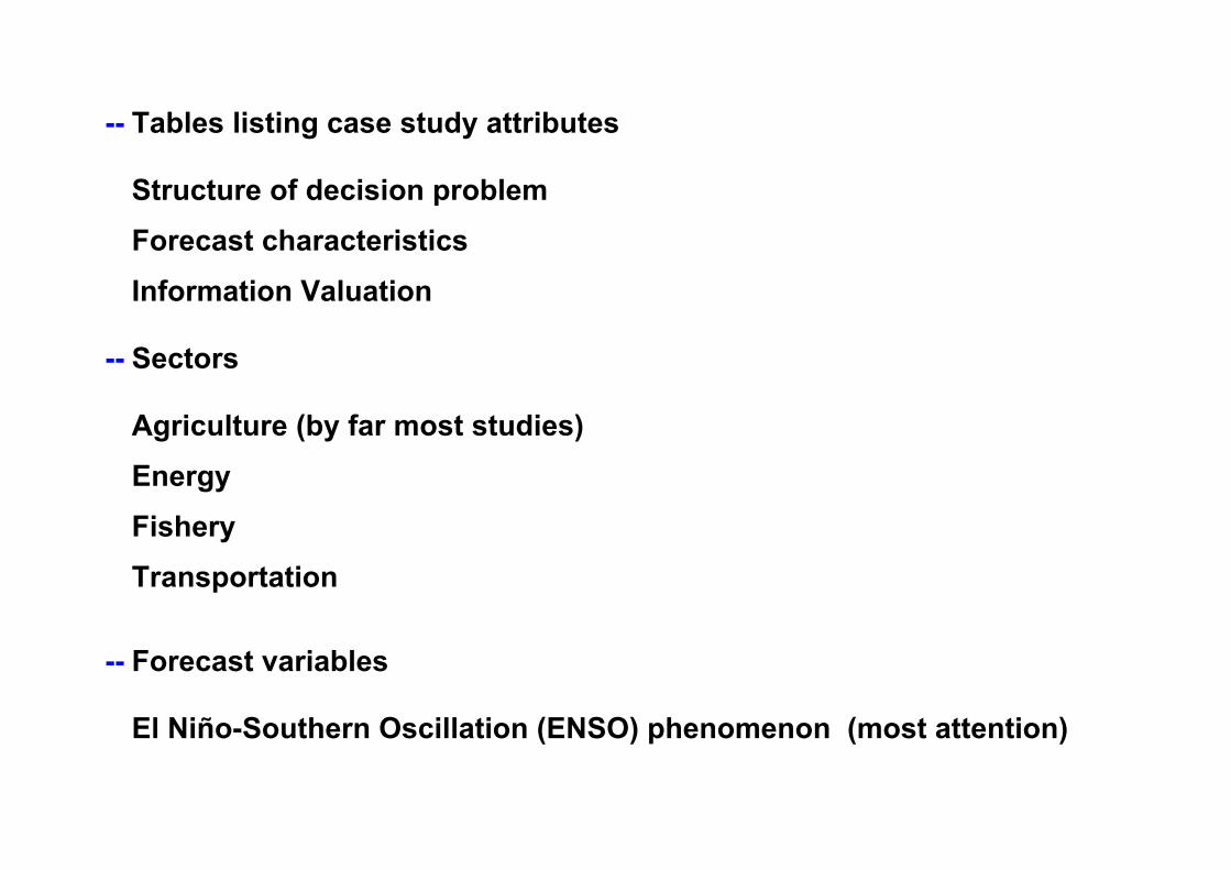
-- Tables listing case study attributes Structure of decision problem Forecast characteristics Information Valuation

-- Sectors

Agriculture (by far most studies) Energy Fishery Transportation

-- Forecast variables El Niño-Southern Oscillation (ENSO) phenomenon (most attention)

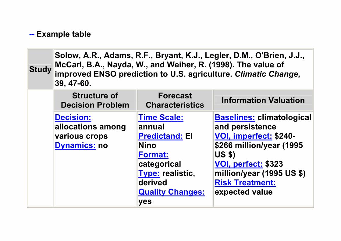
-- Example table

StudySolow, A.R., Adams, R.F., Bryant, K.J., Legler, D.M., O'Brien, J.J., McCarl, B.A., Nayda, W., and Weiher, R. (1998). The value of improved ENSO prediction to U.S. agriculture. Climatic Change, 39, 47-60.

Structure of Decision Problem

Forecast Characteristics Information Valuation

Decision: allocations among various crops Dynamics: no

Time Scale: annual Predictand: El Nino Format: categorical Type: realistic, derived Quality Changes: yes

Baselines: climatological and persistence VOI, imperfect: $240-$266 million/year (1995 US $) VOI, perfect: $323 million/year (1995 US $) Risk Treatment: expected value

(8) Discussion

• Potential Value of Weather Forecasts

-- Fairly well established Wide variety of situations

• Realized Value of Weather Forecasts -- Very limited study Comparison with contingent valuation results (problematic) Descriptive case studies (rarely result in quantitative estimates of forecast value)